ESTIMATION OF MEASUREMENT UNCERTAINTY (Electrical … · ESTIMATION OF MEASUREMENT UNCERTAINTY...

JAB RL504:2013

Initial edition: 2003-03-25 1/33 2nd edition: 2013-01-25

JAB NOTE4

ESTIMATION OF MEASUREMENT UNCERTAINTY

(Electrical Testing / High Power Testing)

2nd edition: January 25 2013 1st edition: March 25 2003

Japan Accreditation Board (JAB)

JAB RL504:2013


JAB NOTE 4 ESTIMATION OF MEASUREMENT UNCERTAINTY

(Electrical Testing/ High Power Testing) January 25, 2013

Accreditation Center Japan Accreditation Board

TABLE OF CONTENTS

1. INTRODUCTION.................................................................................................................................................................... 3 2. SCOPE................................................................................................................................................................................... 3 3. REFERENCES....................................................................................................................................................................... 3 4. TERMS AND DEFINITIONS................................................................................................................................................... 3 5. PRINCIPLES FOR THE ESTIMATION OF UNCERTAINTY .................................................................................................. 6

5.1 Concept of uncertainty..................................................................................................................................................... 6 5.2 Method for evaluating uncertainty.................................................................................................................................... 6 5.3 Type A evaluation of standard uncertainty ....................................................................................................................... 7 5.4 Type B evaluation of standard uncertainty....................................................................................................................... 7 5.5 Calculation of combined standard uncertainty................................................................................................................. 8 5.6 Calculation of expanded uncertainty and rounding.......................................................................................................... 9 5.7 Expression of results ..................................................................................................................................................... 10

6. GUIDELINES FOR THE ESTIMATION OF UNCERTAINTY IN HIGH POWER TESTING .................................................. 12 6.1 Structures of high current measuring systems .............................................................................................................. 12 6.2 Factors contributing to uncertainty in a high current measuring system........................................................................ 14 6.2.1 u1 through u10 - Detector(shunt / CT)....................................................................................................................... 15 6.2.2 u11 through u114 - Transmission system.................................................................................................................... 18 6.2.3 u15 through u17 - Amplifier ........................................................................................................................................ 19 6.2.4 u18 and u19 - Converter............................................................................................................................................. 20 6.2.5 u20 and u21 - Data processing .................................................................................................................................. 21 6.3 Uncertainty budget (Case 1).......................................................................................................................................... 24 6.4 Uncertainty budget (Case 2).......................................................................................................................................... 25 6.5 Uncertainty budget (Case 3).......................................................................................................................................... 26 6.6 Uncertainty budget (Case 4).......................................................................................................................................... 27

7. CLOSURE............................................................................................................................................................................ 28 ADDENDUM 1 REQUIREMENTS FOR MEASUREMENT UNCERTAINTY IN ISO/IEC 17025 .............................................. 29 ADDENDUM 2 STANDARD DEVIATION OF RECTANGULAR DISTRIBUTION..................................................................... 31

JAB RL504:2013


1. INTRODUCTION

The method of estimating “uncertainty" in laboratories for high power testing, with focus on the measurement of values relative to electric current, has been studied. The basic principles of the estimation of uncertainty and its method for high power testing are not different from the one for other test fields. However, once it comes down to their application to practical cases, it is possible to encounter several kinds of alternatives in interpretation in terms of how to apply calculation formulas, etc. This document describes the general principles for estimating the uncertainty in a high current measuring system and is also intended for use in high power testing laboratories, for which cases of measurement instruments and tools actually used in high power testing are addressed and specific examples of the estimation of uncertainty in measurement using such instruments are given.

2. SCOPE

This document applies to the estimation of uncertainty and its evaluation in a high current measuring system and measurement results in high power testing laboratories or laboratories under application for accreditation.

3. REFERENCES

1 ISO/IEC 17025:2005, General requirements for the competence of testing and calibration laboratories

2 ISO/IEC Guide 2:2004, Standardization and related activities-- General vocabulary

3 International vocabulary of metrology-Basic and general concept and associated terms: 2008, issued by

BIPM, IEC, ISO, IFCC, IUPAC, IUPAP and OIML (abbr. VIM)

4 Guide to the Expression of Uncertainty in Measurement: 1995, issued by BIPM, IEC, ISO, IFCC, IUPAC,

IUPAP and OIML (abbr. GUM)

5 IEC 60060-1:2010, High-voltage test techniques. Part 1: General definitions and test requirements

6 IEC 60060-2:2010, High voltage test techniques. Part 2: Measuring systems

7 IEC 62475:2010, High-current test techniques – Definitions and requirements for test currents and

measuring systems

8 CIGRE 33-96 (WG 03):1996, Uncertainty of HV Measurements - the Situation at IEC and CENELEC

9 STL GUIDE TO THE INTERPRETATION OF IEC 60060-2, 1999-11

10 Beginners’ Guide on Uncertainty of Measurement (NITE International Accreditation Japan)

11 JIS Z8101-1:1999, Statistics -- Vocabulary and symbols -- Part 1: Probability and general statistical terms

4. TERMS AND DEFINITIONS

- measurand (VIM 2.6)

particular quantity subject to measurement.

--- true value (VIM 1.19)

value consistent with the definition of a given particular quantity.

- error (in measurement) (VIM 3.10)

result of a measurement minus a true value of the measurand.

- uncertainty of measurement (VIM 3.9)

parameter, associated with the result of a measurement, that characterizes the dispersion of the values that

could reasonably be attributed to the measurand.

- test (ISO/IEC Guide 2)

technical operation that consists of the determination of one or more characteristics of a given product, process

JAB RL504:2013


or service according to a specified procedure.

- calibration (VIM 6.11)

set of operations that establish, under specified conditions, the relationship between values of quantities

indicated by a measuring instrument or measuring system, or values represented by a material measure or a

reference material, and the corresponding values realized by standards.

- resolution

minimum significant identifiable difference (e.g., a change by “1" of the last digit on a digital display)

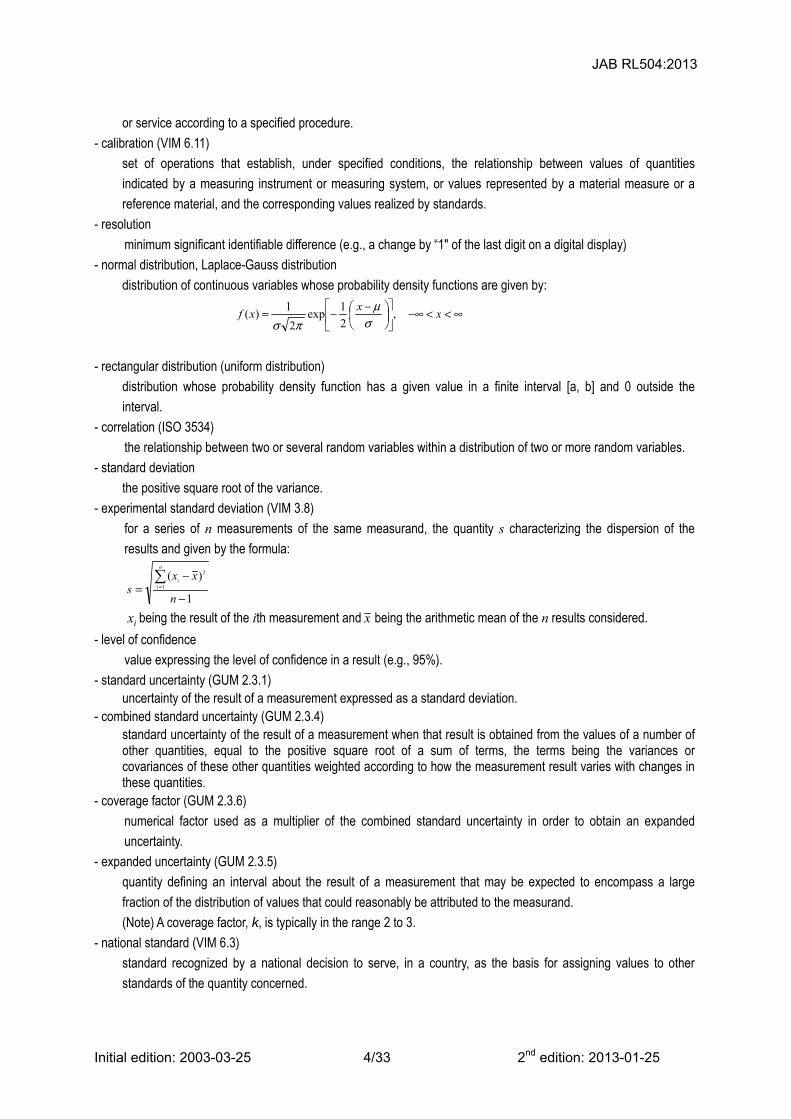
- normal distribution, Laplace-Gauss distribution

distribution of continuous variables whose probability density functions are given by:

,2

1exp

2

1)(

−−=

σμ

πσxxf ∞<<−∞ x

- rectangular distribution (uniform distribution)

distribution whose probability density function has a given value in a finite interval [a, b] and 0 outside the

interval.

- correlation (ISO 3534)

the relationship between two or several random variables within a distribution of two or more random variables.

- standard deviation

the positive square root of the variance.

- experimental standard deviation (VIM 3.8)

for a series of n measurements of the same measurand, the quantity s characterizing the dispersion of the

results and given by the formula:

1

)(1

2

−

−=

=

n

xxs

n

ii

ix being the result of the ith measurement and x being the arithmetic mean of the n results considered.

- level of confidence

value expressing the level of confidence in a result (e.g., 95%).

- standard uncertainty (GUM 2.3.1) uncertainty of the result of a measurement expressed as a standard deviation.

- combined standard uncertainty (GUM 2.3.4) standard uncertainty of the result of a measurement when that result is obtained from the values of a number of other quantities, equal to the positive square root of a sum of terms, the terms being the variances or covariances of these other quantities weighted according to how the measurement result varies with changes in these quantities.

- coverage factor (GUM 2.3.6)

numerical factor used as a multiplier of the combined standard uncertainty in order to obtain an expanded

uncertainty.

- expanded uncertainty (GUM 2.3.5)

quantity defining an interval about the result of a measurement that may be expected to encompass a large

fraction of the distribution of values that could reasonably be attributed to the measurand.

(Note) A coverage factor, k, is typically in the range 2 to 3.

- national standard (VIM 6.3)

standard recognized by a national decision to serve, in a country, as the basis for assigning values to other

standards of the quantity concerned.

JAB RL504:2013


- reference standard (VIM 6.6)

standard, generally having the highest metrological quality available at a given location or in a given organization,

from which measurements made there are derived.

- traceability (VIM 6.10)

property of the result of a measurement or the value of a standard whereby it can be related to stated references,

usually national or international standards, through an unbroken chain of comparisons all having stated

uncertainties.

(Note) The concept is often expressed by the adjective traceable.

- measuring system (VIM 4.5)

complete set of measuring instruments and other equipment assembled to carry out specified measurements.

- rss (root sum square) method a calculation method for obtaining a combined standard uncertainty by combining components that contribute to uncertainty of measurements, this is sometimes called as such because the calculation involves a root sum square of each component by the rule of uncertainty propagation.

Example: 7632 222 =++

- output quantity

a designation of a measurand in the process of its derivation, in most cases, the measurand is not directly

measured, and is determined through functional relation of other more than one quantity, and is called “output

quantity" in the sense that it is the output of the process by the function.

- input quantity (-ies)

quantity measured directly to obtain an output quantity and quantity determined through reference, estimation,

etc., the input usually is normally in plural and an output quantity is determined on input quantities by functional

relationship.

JAB RL504:2013


5. PRINCIPLES FOR THE ESTIMATION OF UNCERTAINTY

5.1 Concept of uncertainty When a measurement is repeated a number of times, even if one thinks that it has been done under the same condition, the resulting values are dispersed. If measured under alternative conditions, e.g. as for the operators, devices or methods, the results will be dispersed due to the changes in conditions. Results are dispersed in a certain range and such range is the uncertainty of measurement. Among conditions of measurement, some are controllable and others not. While conducting a measurement, all or a part of the former (controllable conditions) is held constant. Conditions that are not held constant (usually, portions beyond the limit of control) bring about uncertainty in measured results. There are three kinds of “measurement uncertainty", standard uncertainty “u", combined standard uncertainty “uc", and expanded uncertainty “U". Values stated in reports of measurement results are, usually, expanded uncertainties. By using expanded uncertainty “U", one can state that a measurement result is expected to fall between y-U and y+U in almost all cases of repeated measurement. The extent of “almost all cases" is determined arbitrarily but in many cases a level of confidence of 95% is adopted, which means if the same measurement is conducted 20 times, it is expected that the results will be within this range 19 times out of the 20.

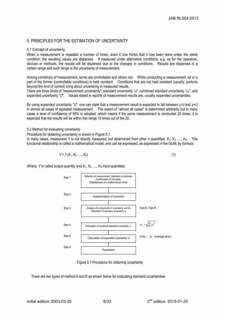
5.2 Method for evaluating uncertainty Procedure for obtaining uncertainty is shown in Figure 5.1. In many cases, measurand Y is not directly measured, but determined from other n quantities: X1, X2, …, XN. This functional relationship is called a mathematical model, and can be expressed, as expressed in the GUM, by formula:

Y = f (X1, X2, …, XN) (1)

Where, Y is called output quantity and X1, X2, …, XN input quantities.

There are two types of method A and B as shown below for evaluating standard uncertainties:

Selection of measurement/ calibration procedures Confirmation of principles

Establishment of a mathematical model

Implementation of correction

Analysis of components of uncertainty and its calculation of standard uncertainty ui

Calculation of combined standard uncertainty uc

Calculation of expanded uncertainty U

Expression

Step 1 Step 2 Step 3 Step 4 Step 5 Step 6

Type A, Type B

= 2ic uu

U=kuc k：coverage factor

Figure 5.1 Procedure for obtaining uncertainty

JAB RL504:2013


Type A: Evaluations by a statistical analysis of the results of a series of repeated measurements. The standard deviation obtained from the statistical analysis is considered as standard uncertainty. Usually, normal distribution (Laplace-Gauss distribution) is presumed.

Type B: Evaluation by methods other than statistical. Attention should be paid to the form of distribution (whether rectangular, normal, etc.).

5.3 Type A evaluation of standard uncertainty In many instances, measurement is repeated several times under the same condition, i.e. to obtain estimated value q of measurand Q , experiments are repeated n times, observed values qi (i = 1, 2,…, n) from each experiment are averaged, and the mean value q is determined to be estimated value q.

=

=n

iiqn

q1

1 (2)

The experimental variance s2(qk) is used as the estimate of the variance σ2 of q.

=

−−

=n

iik qq

nqs

1

22 )(1

1)( (3)

The positive square root of the experimental variance is the experimental standard deviation s(qk). In this case, the degree of freedom of the experimental standard deviation is n-1.

The variance of the mean q is given by n

q2

2 )(σσ = . Therefore, (4) is used as its estimated value:

nqsqs k )(

)(2

2 = (4)

Where, )(2 qs is called the experimental variance of the mean, and its positive square root )(qs the experimental standard deviation of the mean. Through the above experiments and statistical analyses, the estimated value q of measurand Q is obtained as the mean value q and its standard uncertainty )(qu as the experimental standard deviation of the mean )(qs . )()( qsqu = (5)

(REMARK 1) There is a procedure to multiply the experimental standard deviation by t-value to get a kind of expanded

uncertainty corresponding to 95% level of confidence and then divide it by 2 followed by the calculation of combined

standard uncertainty. This is not a procedure prescribed in the GUM and should not be used.

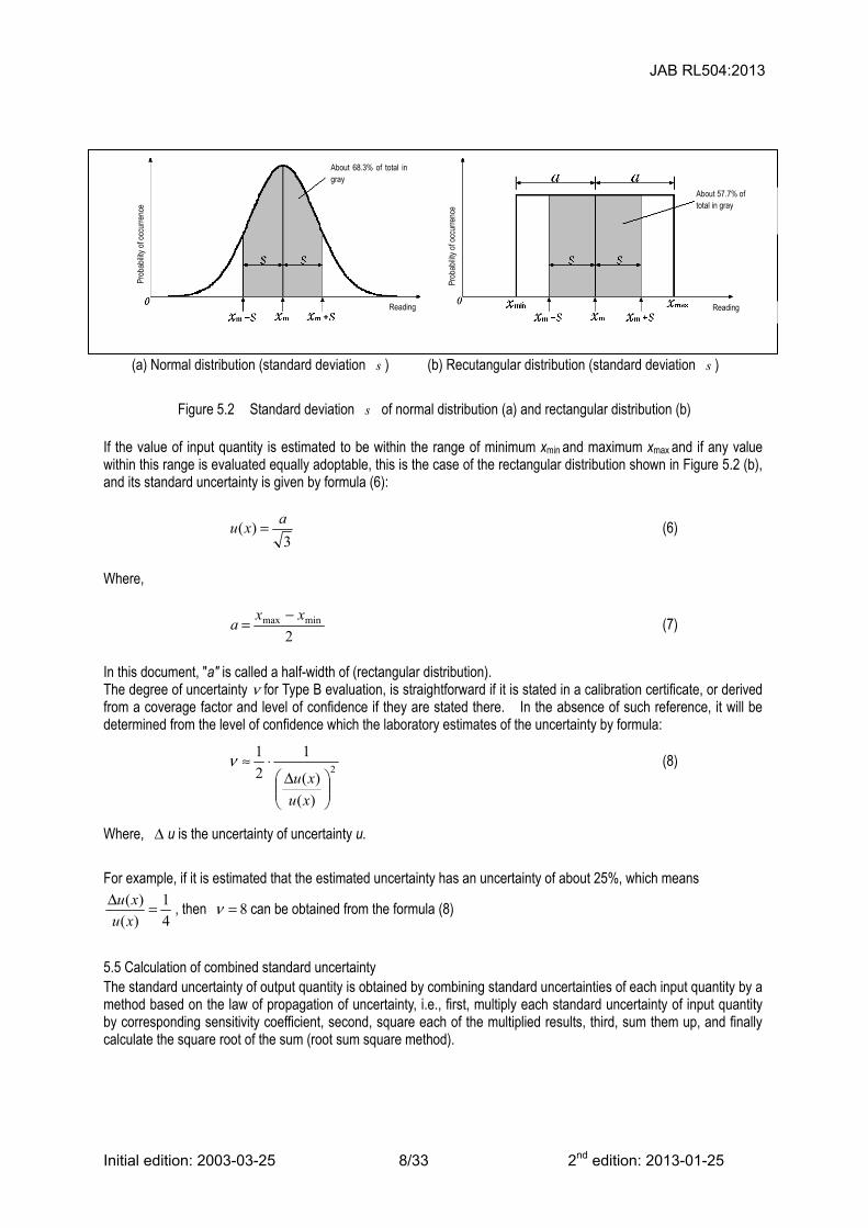
5.4 Type B evaluation of standard uncertainty The standard uncertainties associated with the estimated values of input quantities that are not from repeated observation will be evaluated through scientific judgments based on all available information. Type of probability distribution, standard uncertainty and, if necessary, degree of freedom should be determined. With regard to the probability distribution, there are normal, rectangular, triangular, trapezoidal, U-shaped, etc., of which the normal and rectangular distributions are most frequently used and illustrated in Figure 5.2.

JAB RL504:2013


(a) Normal distribution (standard deviation s ) (b) Recutangular distribution (standard deviation s )

Figure 5.2 Standard deviation s of normal distribution (a) and rectangular distribution (b)

If the value of input quantity is estimated to be within the range of minimum xmin and maximum xmax and if any value within this range is evaluated equally adoptable, this is the case of the rectangular distribution shown in Figure 5.2 (b), and its standard uncertainty is given by formula (6):

3

)(axu = (6)

Where,

2

minmax xxa −= (7)

In this document, "a" is called a half-width of (rectangular distribution). The degree of uncertainty ν for Type B evaluation, is straightforward if it is stated in a calibration certificate, or derived from a coverage factor and level of confidence if they are stated there. In the absence of such reference, it will be determined from the level of confidence which the laboratory estimates of the uncertainty by formula:

2

)(

)(

1

2

1

Δ⋅≈

xuxu

ν (8)

Where, Δ u is the uncertainty of uncertainty u.

For example, if it is estimated that the estimated uncertainty has an uncertainty of about 25%, which means

4

1

)(

)( =Δxuxu

, then 8=ν can be obtained from the formula (8)

5.5 Calculation of combined standard uncertainty The standard uncertainty of output quantity is obtained by combining standard uncertainties of each input quantity by a method based on the law of propagation of uncertainty, i.e., first, multiply each standard uncertainty of input quantity by corresponding sensitivity coefficient, second, square each of the multiplied results, third, sum them up, and finally calculate the square root of the sum (root sum square method).

About 68.3% of total in gray

About 57.7% of total in gray

Reading Reading

Prob

abilit

y of

occ

urre

nce

Prob

abilit

y of

occ

urre

nce

JAB RL504:2013


[ ]2

1

)()( =

=n

iiic xucyu (9)

Where u(xi) is the standard uncertainty of the ith input quantity Xi ; ci is the sensitivity coefficient of Y to Xi .

Sensitivity coefficient may be obtained from the formula (1) by its partial derivative iXf

∂∂

at Xi =xi. In cases where

the form of mathematical function is not clear, it can be obtained experimentally, i.e., change xi by a small amount Δ xi in the neighborhood of Xi =xi and observe the corresponding change Δ y of Y, and then calculate by formula (10):

i

i xyc

ΔΔ= (10)

(NOTE 1) The formula (9) is for the case where there is no correlation among input quantities. For the case where

input quantities are correlated, please refer to the GUM etc.

(NOTE 2) The formula (9) is for an uncertainty in absolute value (not a relative value). When the function of the

mathematical model is the product (including quotient) of input quantities, the direct use of formula (9) makes the

calculation complicated. In such case, modification of the formula (9) paying attention to factors contained in sensitivity

coefficients leads to a formula of a simple root sum square method for relative uncertainty.

(NOTE 3) Calculation of combined standard uncertainty may be divided in several steps. Especially, when there exist

more than one component contributing to the uncertainty of a certain input quantity, it is desirable to obtain the

standard uncertainty of the input quantity by combining the standard uncertainties of its components. Such process will

make the whole procedure of uncertainty evaluation easy to grasp. In the example of uncertainty calculation shown at

6.2, rss method is used to relative uncertainty and standard uncertainty of each component are combined.

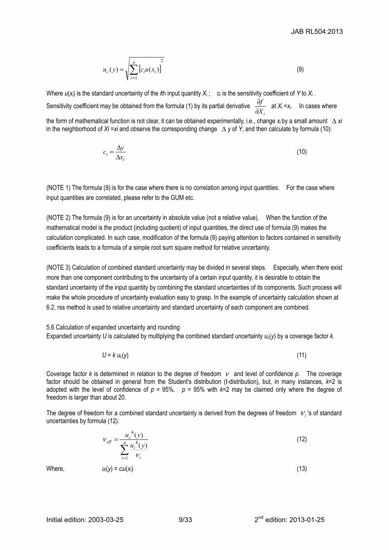
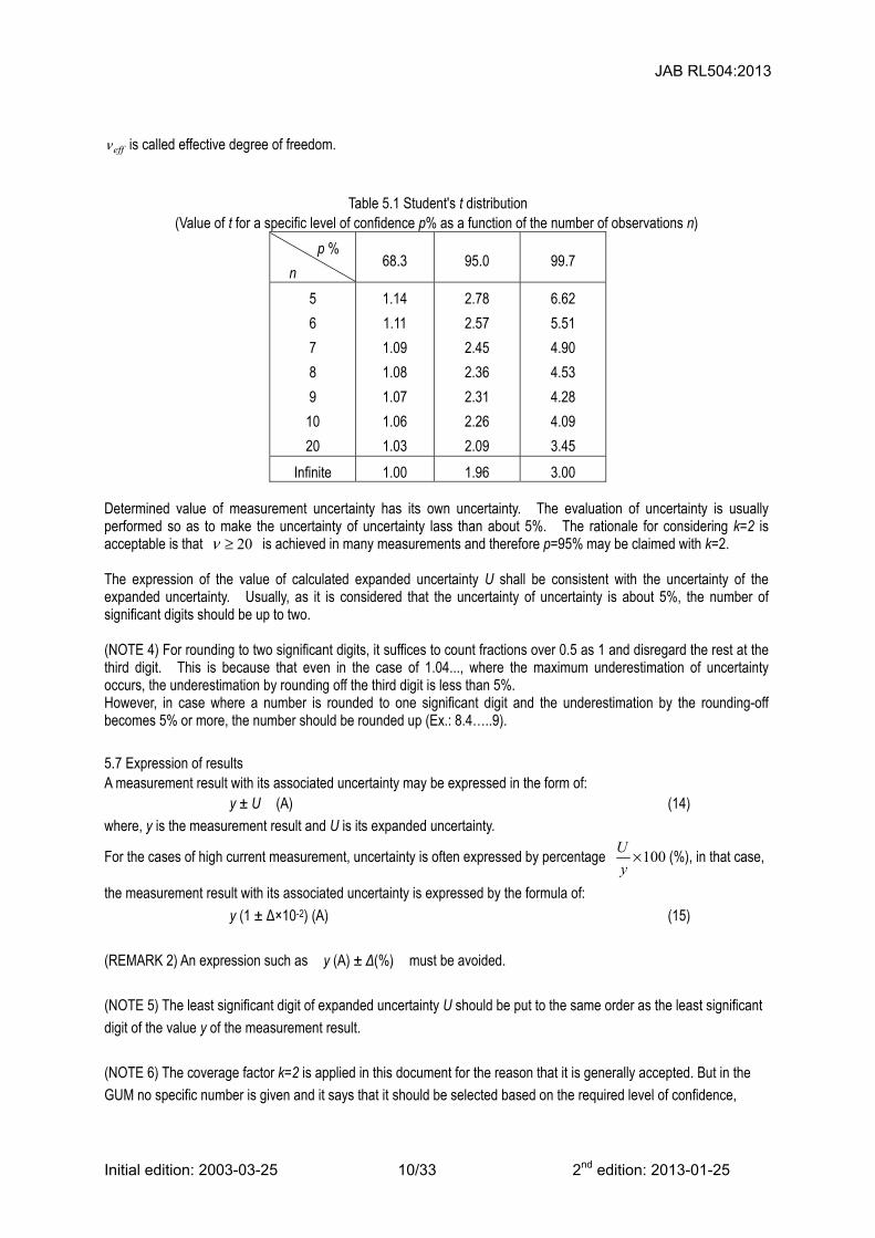
5.6 Calculation of expanded uncertainty and rounding Expanded uncertainty U is calculated by multiplying the combined standard uncertainty uc(y) by a coverage factor k.

U = k uc(y) (11)

Coverage factor k is determined in relation to the degree of freedom ν and level of confidence p. The coverage factor should be obtained in general from the Student's distribution (t-distribution), but, in many instances, k=2 is adopted with the level of confidence of p = 95%. p = 95% with k=2 may be claimed only where the degree of freedom is larger than about 20. The degree of freedom for a combined standard uncertainty is derived from the degrees of freedom iν 's of standard uncertainties by formula (12):

=

= n

i i

i

ceff yu

yu

1

4

4

)(

)(

ν

ν (12)

Where, ui(y) = ciu(xi) (13)

JAB RL504:2013


effν is called effective degree of freedom.

Table 5.1 Student's t distribution (Value of t for a specific level of confidence p% as a function of the number of observations n)

p %

n 68.3 95.0 99.7

5

6

7

8

9

10

20

1.14

1.11

1.09

1.08

1.07

1.06

1.03

2.78

2.57

2.45

2.36

2.31

2.26

2.09

6.62

5.51

4.90

4.53

4.28

4.09

3.45

Infinite 1.00 1.96 3.00

Determined value of measurement uncertainty has its own uncertainty. The evaluation of uncertainty is usually performed so as to make the uncertainty of uncertainty lass than about 5%. The rationale for considering k=2 is acceptable is that 20≥ν is achieved in many measurements and therefore p=95% may be claimed with k=2. The expression of the value of calculated expanded uncertainty U shall be consistent with the uncertainty of the expanded uncertainty. Usually, as it is considered that the uncertainty of uncertainty is about 5%, the number of significant digits should be up to two. (NOTE 4) For rounding to two significant digits, it suffices to count fractions over 0.5 as 1 and disregard the rest at the third digit. This is because that even in the case of 1.04..., where the maximum underestimation of uncertainty occurs, the underestimation by rounding off the third digit is less than 5%. However, in case where a number is rounded to one significant digit and the underestimation by the rounding-off becomes 5% or more, the number should be rounded up (Ex.: 8.4…..9).

5.7 Expression of results A measurement result with its associated uncertainty may be expressed in the form of:

y ± U (A) (14)

where, y is the measurement result and U is its expanded uncertainty.

For the cases of high current measurement, uncertainty is often expressed by percentage 100×yU

(%), in that case,

the measurement result with its associated uncertainty is expressed by the formula of:

y (1 ± Δ×10-2) (A) (15)

(REMARK 2) An expression such as y (A) ± Δ(%) must be avoided.

(NOTE 5) The least significant digit of expanded uncertainty U should be put to the same order as the least significant

digit of the value y of the measurement result.

(NOTE 6) The coverage factor k=2 is applied in this document for the reason that it is generally accepted. But in the

GUM no specific number is given and it says that it should be selected based on the required level of confidence,

JAB RL504:2013


saying also that, in general, the number is between 2 and 3. Anyway the value given to k needs to be stated together

with the value of uncertainty. Furthermore, if possible, the degree of freedom and level of confidence should also be

stated.

(Example: XX±YY (A), where the number following symbol ± is the number value of an expanded uncertainty, determined from a coverage factor k=2 based on the t-distribution for ν =50 degrees of freedom, and defines an

interval estimated to have a level of confidence of 95%.)

JAB RL504:2013


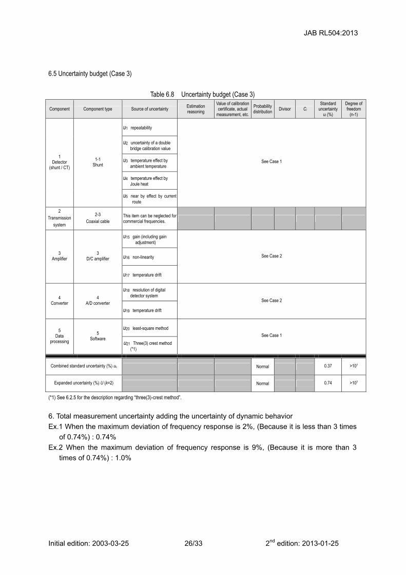
6. GUIDELINES FOR THE ESTIMATION OF UNCERTAINTY IN HIGH POWER TESTING

6.1 Structures of high current measuring systems

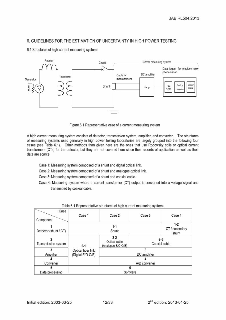
Figure 6.1 Representative case of a current measuring system

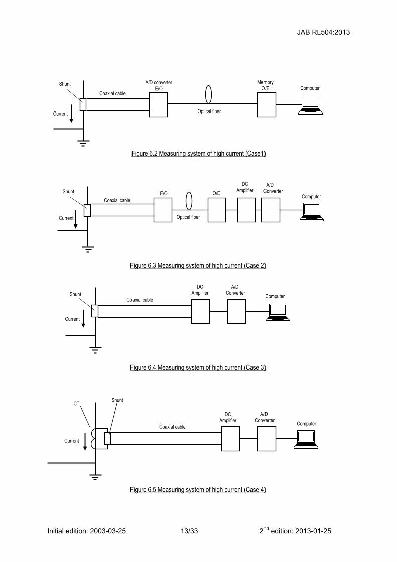
A high current measuring system consists of detector, transmission system, amplifier, and converter. The structures of measuring systems used generally in high power testing laboratories are largely grouped into the following four cases (see Table 6.1). Other methods than given here are the ones that use Rogowsky coils or optical current transformers (CTs) for the detector, but they are not covered here since their records of application as well as their data are scarce.

Case 1: Measuring system composed of a shunt and digital optical link.

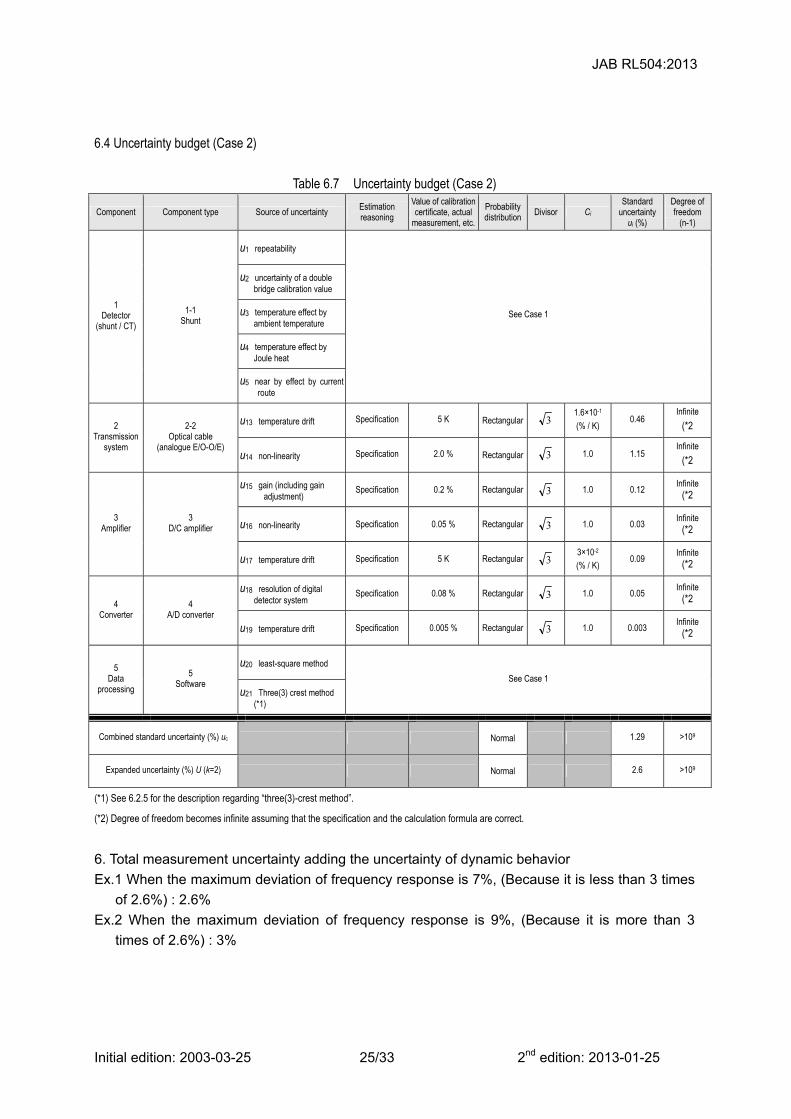
Case 2: Measuring system composed of a shunt and analogue optical link.

Case 3: Measuring system composed of a shunt and coaxial cable.

Case 4: Measuring system where a current transformer (CT) output is converted into a voltage signal and

transmitted by coaxial cable.

Table 6.1 Representative structures of high current measuring systems Case

Component

Case 1 Case 2 Case 3 Case 4

1 Detector (shunt / CT)

1-1 Shunt

1-2 CT / secondary

shunt

2 Transmission system

2-2 Optical cable

(Analogue E/O-O/E)

2-3 Coaxial cable

3 Amplifier

3 DC amplifier

4 Converter

2-1 Optical fiber link (Digital E/O-O/E)

4 A/D converter

5 Data processing

5 Software

Generator Transformer

Circuit

Cable formeasurement

DC amplifier

Current measuring system Reactor

Shunt

Data logger for medium/ slow phenomenon

Memory media

Conversion

JAB RL504:2013


Figure 6.2 Measuring system of high current (Case1)

Figure 6.3 Measuring system of high current (Case 2)



CT

Coaxial cable Computer

A/DConverter

DCAmplifier

Current

Shunt

Current

E/O

Optical fiber

A/DConverter

DCAmplifier O/E

Computer Coaxial cable

Current

Shunt

Optical fiber

Computer Memory

O/E A/D converter

E/O Coaxial cable

Current

Shunt Coaxial cable

DCAmplifier

A/DConverter

Computer

Shunt

JAB RL504:2013


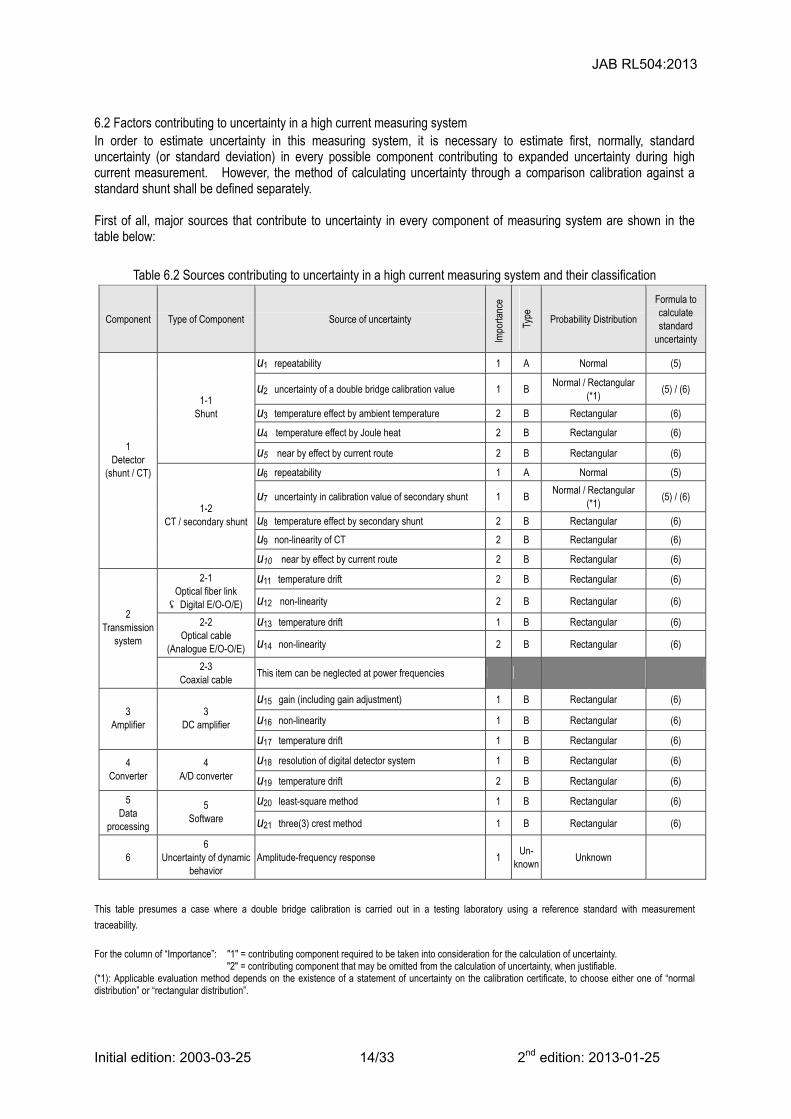
6.2 Factors contributing to uncertainty in a high current measuring system In order to estimate uncertainty in this measuring system, it is necessary to estimate first, normally, standard uncertainty (or standard deviation) in every possible component contributing to expanded uncertainty during high current measurement. However, the method of calculating uncertainty through a comparison calibration against a standard shunt shall be defined separately. First of all, major sources that contribute to uncertainty in every component of measuring system are shown in the table below:

Table 6.2 Sources contributing to uncertainty in a high current measuring system and their classification

Component Type of Component Source of uncertainty

Impo

rtanc

e

Type

Probability Distribution

Formula to calculate standard

uncertainty

u1 repeatability 1 A Normal (5)

u2 uncertainty of a double bridge calibration value 1 B Normal / Rectangular

(*1) (5) / (6)

u3 temperature effect by ambient temperature 2 B Rectangular (6)

u4 temperature effect by Joule heat 2 B Rectangular (6)

1-1 Shunt

u5 near by effect by current route 2 B Rectangular (6)

u6 repeatability 1 A Normal (5)

u7 uncertainty in calibration value of secondary shunt 1 B Normal / Rectangular

(*1) (5) / (6)

u8 temperature effect by secondary shunt 2 B Rectangular (6)

u9 non-linearity of CT 2 B Rectangular (6)

1 Detector

(shunt / CT)

1-2 CT / secondary shunt

u10 near by effect by current route 2 B Rectangular (6)

u11 temperature drift 2 B Rectangular (6) 2-1 Optical fiber link （Digital E/O-O/E) u12 non-linearity 2 B Rectangular (6)

u13 temperature drift 1 B Rectangular (6) 2-2 Optical cable

(Analogue E/O-O/E) u14 non-linearity 2 B Rectangular (6)

2 Transmission

system

2-3 Coaxial cable

This item can be neglected at power frequencies

u15 gain (including gain adjustment) 1 B Rectangular (6)

u16 non-linearity 1 B Rectangular (6) 3

Amplifier 3

DC amplifier

u17 temperature drift 1 B Rectangular (6)

u18 resolution of digital detector system 1 B Rectangular (6) 4 Converter

4 A/D converter u19 temperature drift 2 B Rectangular (6)

u20 least-square method 1 B Rectangular (6) 5 Data

processing

5 Software u21 three(3) crest method 1 B Rectangular (6)

6 6

Uncertainty of dynamic behavior

Amplitude-frequency response 1 Un-

knownUnknown

This table presumes a case where a double bridge calibration is carried out in a testing laboratory using a reference standard with measurement

traceability.

For the column of “Importance”: "1" = contributing component required to be taken into consideration for the calculation of uncertainty.

"2" = contributing component that may be omitted from the calculation of uncertainty, when justifiable. (*1): Applicable evaluation method depends on the existence of a statement of uncertainty on the calibration certificate, to choose either one of “normal distribution” or “rectangular distribution”.

JAB RL504:2013


Using the identification numbers shown in Table 6.2, factors of uncertainty for each component and examples of the calculation of standard uncertainty are shown below:

6.2.1 u1 through u10 - Detector(shunt / CT)

6.2.1.1 u1 through u5 - Shunt Shunt is a resistive element that converts current into voltage, and in order to e exclude reactance component as much for accurate measurement, coaxial type shunts with least inductance are generally applied in high current measuring. The uncertainty of a shunt relates to its resistance, where uncertainties by its resistance measurement, surrounding temperature, temperature rise by Joule heat, etc, introduce effects. In designing shunt, usually, material with minimum temperature coefficient is applied, so as to satisfy the thermal capacity specification regarding the temperature rise.

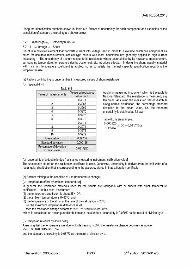
(a) Factors contributing to uncertainties in measured values of shunt resistance

[u1 repeatability] Table 6.3

Times of measurements Measured resistance

value (mΩ) 1 0.3971 2 0.3968 3 0.3969 4 0.3970 5 0.3970 6 0.3970 7 0.3971 8 0.3971 9 0.3972 10 0.3972

Mean value 0.39704 Standard deviation 0.000126

Percentage of deviation to mean value 0.0317(%)

Applying measuring instrument which is traceable to National Standard, the resistance is measured, e.g. ten times. Assuming the measured values distribute along normal distribution, the percentage standard deviation to the mean value, i.e. the standard uncertainty is obtained as follows: Table 6.3 is an example.

(%)0317.010039704.0

000126.0 =×

[u2 uncertainty of a double bridge (resistance measuring instrument) calibration value] The uncertainty stated on the calibration certificate is used. Otherwise, uncertainty is derived from the half-width of a rectangular distribution that is corresponding to the accuracy stated in that calibration certificate.

(b) Factors relating to the condition of use (temperature change)

[u3 temperature effect by ambient temperature] In general, the resistance materials used for the shunts are Manganin wire or sheets with small temperature coefficients. In this case, if assumed: (1) the temperature coefficient is about 25×10-6 , (2) the ambient temperature is 0~40ºC, and (3) the temperature of the shunt at the time of the calibration is 20ºC,

i.e. the maximum temperature difference is 20K, then the resistance change becomes: 25×10-6×20=0.0005 (=0.05%),

which is considered as rectangular distribution and the standard uncertainty is 0.029% as the result of division by 3 .

[u4 temperature effect by Joule heat] Assuming that the temperature rise due to Joule heating is 60K, the resistance change becomes as above: 25×10-6×60=0.0015 (=0.15%), and the standard uncertainty is 0.087% as the result of division by 3 .

JAB RL504:2013


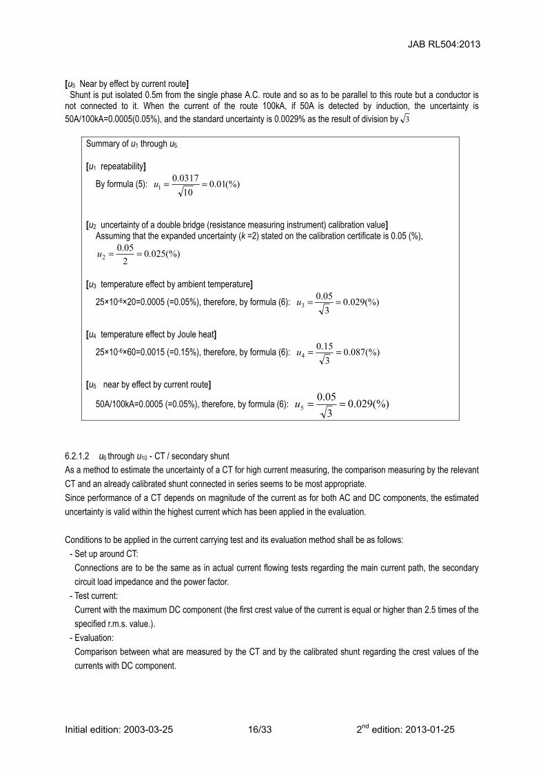
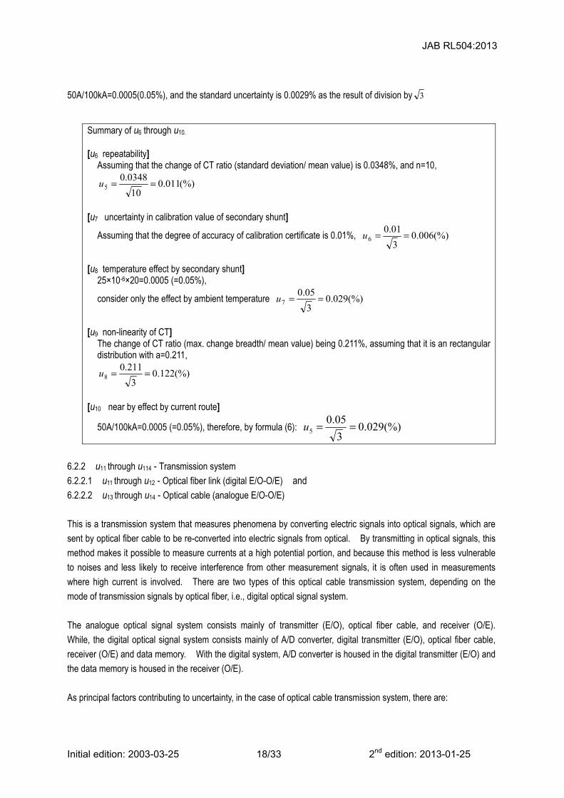
[u5 Near by effect by current route] Shunt is put isolated 0.5m from the single phase A.C. route and so as to be parallel to this route but a conductor is

not connected to it. When the current of the route 100kA, if 50A is detected by induction, the uncertainty is 50A/100kA=0.0005(0.05%), and the standard uncertainty is 0.0029% as the result of division by 3

Summary of u1 through u5. [u1 repeatability]

By formula (5): (%)01.010

0317.01 ==u

[u2 uncertainty of a double bridge (resistance measuring instrument) calibration value]

Assuming that the expanded uncertainty (k =2) stated on the calibration certificate is 0.05 (%),

(%)025.02

05.02 ==u

[u3 temperature effect by ambient temperature]

25×10-6×20=0.0005 (=0.05%), therefore, by formula (6): (%)029.03

05.03 ==u

[u4 temperature effect by Joule heat]

25×10-6×60=0.0015 (=0.15%), therefore, by formula (6): (%)087.03

15.04 ==u

[u5 near by effect by current route]

50A/100kA=0.0005 (=0.05%), therefore, by formula (6): (%)029.03

05.05 ==u

6.2.1.2 u6 through u10 - CT / secondary shunt As a method to estimate the uncertainty of a CT for high current measuring, the comparison measuring by the relevant

CT and an already calibrated shunt connected in series seems to be most appropriate.

Since performance of a CT depends on magnitude of the current as for both AC and DC components, the estimated

uncertainty is valid within the highest current which has been applied in the evaluation.

Conditions to be applied in the current carrying test and its evaluation method shall be as follows:

- Set up around CT:

Connections are to be the same as in actual current flowing tests regarding the main current path, the secondary

circuit load impedance and the power factor.

- Test current:

Current with the maximum DC component (the first crest value of the current is equal or higher than 2.5 times of the

specified r.m.s. value.).

- Evaluation:

Comparison between what are measured by the CT and by the calibrated shunt regarding the crest values of the

currents with DC component.

JAB RL504:2013


[u6 repeatability] Using a traceable AC shunt connected in series to a CT, the same electric current is loaded n times. From the mean

value and the standard deviation of those n measurements the percentile deviation of CT ratio is obtained to derive a

standard uncertainty assuming they are in normal distribution. Estimation is made by the comparison of the first

peak of the loaded current.

Table 6.4 shows an example of measurements and evaluation results.

Table 6.4 Example of measurements by a CT and a shunt for

comparison connected in a series. (repeatability) Alternate current shunt

measured values Im [kA]

CT measured value Ii [kA]

Ratio ( = Ii / Im )

53.05 52.63 0.9921 57.30 56.90 0.9930 53.17 52.74 0.9919 57.39 56.97 0.9927 53.13 52.73 0.9925 57.24 56.82 0.9927 53.32 52.90 0.9921 57.49 57.06 0.9925 52.97 52.58 0.9926 57.40 56.95 0.9922

Average of ratios: 0.9924 Standard deviation: 0.000345 Uncertainty of CT ratio:

(%)0348.01009924.0

000345.0 =×

[u7 uncertainty in calibration value of secondary shunt]

Same as u2.

[u8 temperature effect by secondary shunt]

Same as u3.

[u9 non-linearity of CT] Using a traceable alternate current shunt connected in a series to a CT, electric current divided approximately in 5

steps within a measurement range is loaded, and the ratio of maximum change breadth from its average value is

obtained, which is assumed as in rectangular distribution, thus deriving standard uncertainty. Estimation is made by

the comparison of the first wave height values of loaded current. Table 6.5 shows an example of measurement

results.

Table 6.5 Example of measurement results of a CT and an alternate

shunt for comparison connected in a series. (non-linearity) Alternate current shunt

measured values Im [kA]

CT measured value Ii [kA]

Ratio (=Ii / Im)

21.61 21.44 0.9921 29.53 29.34 0.9936 36.11 35.91 0.9945 44.96 44.77 0.9958 55.88 55.45 0.9923

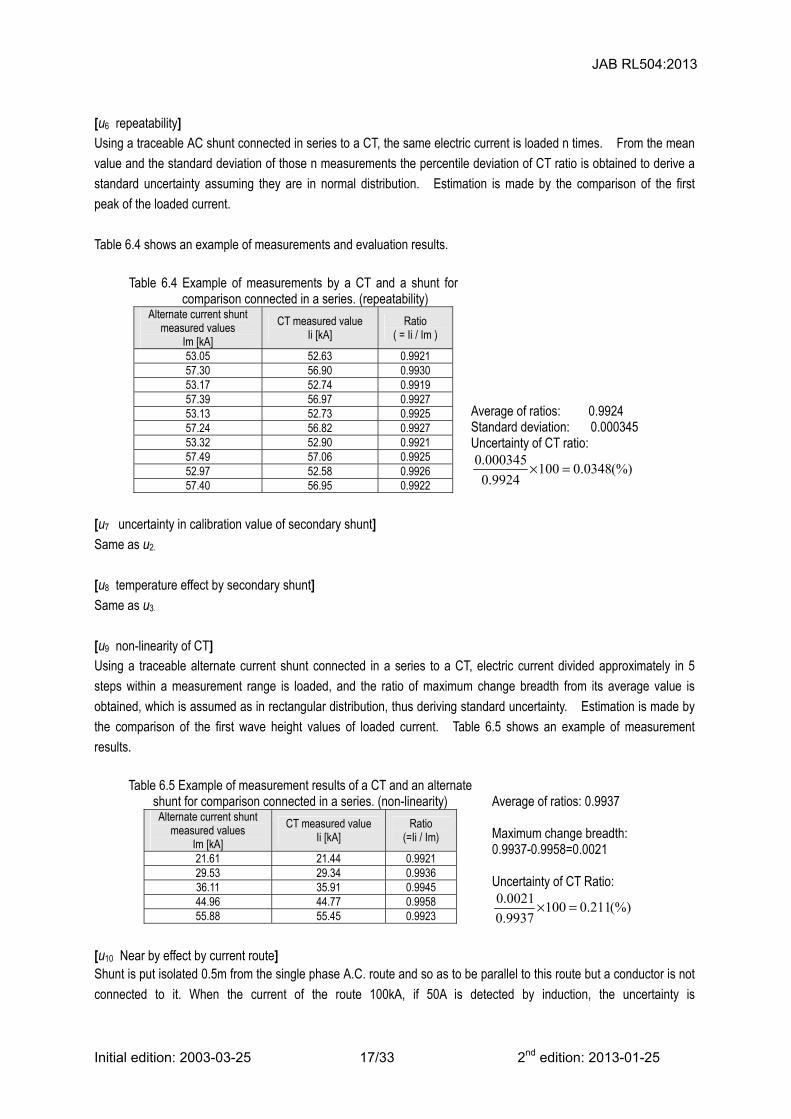
Average of ratios: 0.9937 Maximum change breadth: 0.9937-0.9958=0.0021 Uncertainty of CT Ratio:

(%)211.01009937.0

0021.0 =×

[u10 Near by effect by current route] Shunt is put isolated 0.5m from the single phase A.C. route and so as to be parallel to this route but a conductor is not

connected to it. When the current of the route 100kA, if 50A is detected by induction, the uncertainty is

JAB RL504:2013


50A/100kA=0.0005(0.05%), and the standard uncertainty is 0.0029% as the result of division by 3

Summary of u6 through u10. [u6 repeatability]

Assuming that the change of CT ratio (standard deviation/ mean value) is 0.0348%, and n=10,

(%)011.010

0348.05 ==u

[u7 uncertainty in calibration value of secondary shunt]

Assuming that the degree of accuracy of calibration certificate is 0.01%, (%)006.03

01.06 ==u

[u8 temperature effect by secondary shunt]

25×10-6×20=0.0005 (=0.05%),

consider only the effect by ambient temperature (%)029.03

05.07 ==u

[u9 non-linearity of CT]

The change of CT ratio (max. change breadth/ mean value) being 0.211%, assuming that it is an rectangular distribution with a=0.211,

(%)122.03

211.08 ==u

[u10 near by effect by current route]

50A/100kA=0.0005 (=0.05%), therefore, by formula (6): (%)029.03

05.05 ==u

6.2.2 u11 through u114 - Transmission system

6.2.2.1 u11 through u12 - Optical fiber link (digital E/O-O/E) and

6.2.2.2 u13 through u14 - Optical cable (analogue E/O-O/E)

This is a transmission system that measures phenomena by converting electric signals into optical signals, which are

sent by optical fiber cable to be re-converted into electric signals from optical. By transmitting in optical signals, this

method makes it possible to measure currents at a high potential portion, and because this method is less vulnerable

to noises and less likely to receive interference from other measurement signals, it is often used in measurements

where high current is involved. There are two types of this optical cable transmission system, depending on the

mode of transmission signals by optical fiber, i.e., digital optical signal system.

The analogue optical signal system consists mainly of transmitter (E/O), optical fiber cable, and receiver (O/E).

While, the digital optical signal system consists mainly of A/D converter, digital transmitter (E/O), optical fiber cable,

receiver (O/E) and data memory. With the digital system, A/D converter is housed in the digital transmitter (E/O) and

the data memory is housed in the receiver (O/E).

As principal factors contributing to uncertainty, in the case of optical cable transmission system, there are:

JAB RL504:2013


･Gain;

･Linearity; and

･Temperature drift.

For the evaluation of these uncertainties, values stated in the calibration certificate of the optical cable transmission

system provided by the manufacturer (if unavailable, its specification will do) of the degree of accuracy, etc. are used

to derive uncertainty of Type B.

Some of the optical cable transmission systems have auto-calibration function that adjusts automatically gains and

temperature drift, in which case, it is possible to evaluate uncertainty taking into consideration the automatic

adjustment function. The analogue optical signal system is comparatively less reliable in its accuracy and mandates

measurements using this function.

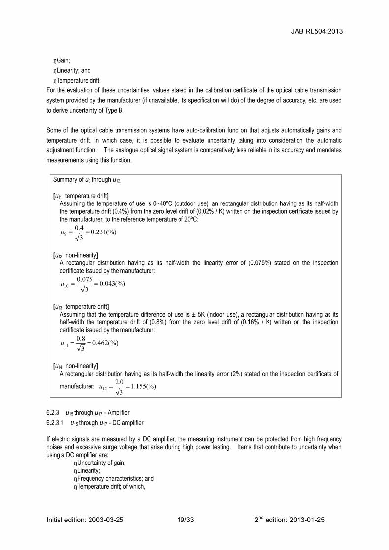
Summary of u9 through u12.

[u11 temperature drift]

Assuming the temperature of use is 0~40ºC (outdoor use), an rectangular distribution having as its half-width the temperature drift (0.4%) from the zero level drift of (0.02% / K) written on the inspection certificate issued by the manufacturer, to the reference temperature of 20ºC:

(%)231.03

4.09 ==u

[u12 non-linearity]

A rectangular distribution having as its half-width the linearity error of (0.075%) stated on the inspection certificate issued by the manufacturer:

(%)043.03

075.010 ==u


Assuming that the temperature difference of use is ± 5K (indoor use), a rectangular distribution having as its half-width the temperature drift of (0.8%) from the zero level drift of (0.16% / K) written on the inspection certificate issued by the manufacturer:

(%)462.03

8.011 ==u

[u14 non-linearity]

A rectangular distribution having as its half-width the linearity error (2%) stated on the inspection certificate of

manufacturer: (%)155.13

0.212 ==u

6.2.3 u15 through u17 - Amplifier

6.2.3.1 u15 through u17 - DC amplifier If electric signals are measured by a DC amplifier, the measuring instrument can be protected from high frequency noises and excessive surge voltage that arise during high power testing. Items that contribute to uncertainty when using a DC amplifier are:

･Uncertainty of gain; ･Linearity; ･Frequency characteristics; and ･Temperature drift; of which,

JAB RL504:2013


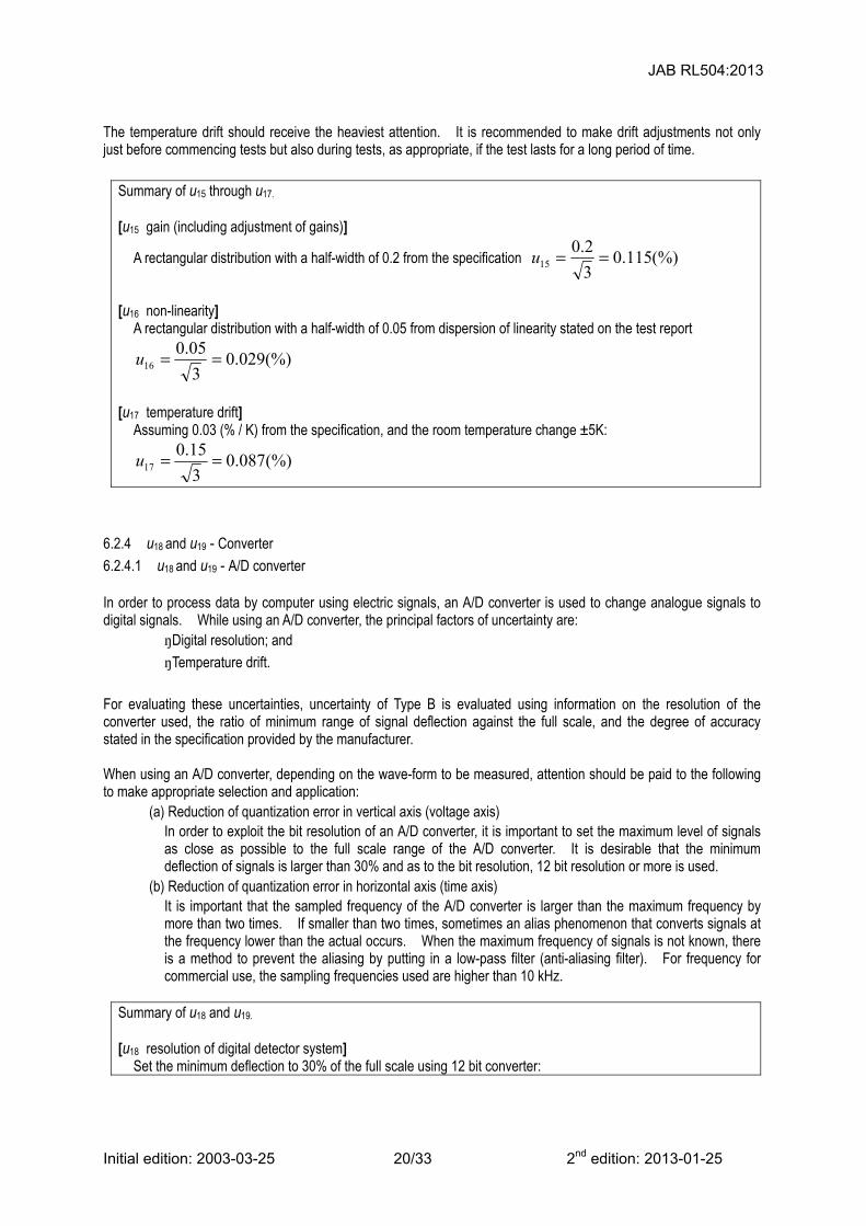
The temperature drift should receive the heaviest attention. It is recommended to make drift adjustments not only just before commencing tests but also during tests, as appropriate, if the test lasts for a long period of time.

Summary of u15 through u17.

[u15 gain (including adjustment of gains)]

A rectangular distribution with a half-width of 0.2 from the specification (%)115.03

2.015 ==u

[u16 non-linearity]

A rectangular distribution with a half-width of 0.05 from dispersion of linearity stated on the test report

(%)029.03

05.016 ==u


Assuming 0.03 (% / K) from the specification, and the room temperature change ±5K:

(%)087.03

15.017 ==u

6.2.4 u18 and u19 - Converter

6.2.4.1 u18 and u19 - A/D converter In order to process data by computer using electric signals, an A/D converter is used to change analogue signals to digital signals. While using an A/D converter, the principal factors of uncertainty are:

･Digital resolution; and

･Temperature drift.

For evaluating these uncertainties, uncertainty of Type B is evaluated using information on the resolution of the converter used, the ratio of minimum range of signal deflection against the full scale, and the degree of accuracy stated in the specification provided by the manufacturer. When using an A/D converter, depending on the wave-form to be measured, attention should be paid to the following to make appropriate selection and application:

(a) Reduction of quantization error in vertical axis (voltage axis) In order to exploit the bit resolution of an A/D converter, it is important to set the maximum level of signals as close as possible to the full scale range of the A/D converter. It is desirable that the minimum deflection of signals is larger than 30% and as to the bit resolution, 12 bit resolution or more is used.

(b) Reduction of quantization error in horizontal axis (time axis) It is important that the sampled frequency of the A/D converter is larger than the maximum frequency by more than two times. If smaller than two times, sometimes an alias phenomenon that converts signals at the frequency lower than the actual occurs. When the maximum frequency of signals is not known, there is a method to prevent the aliasing by putting in a low-pass filter (anti-aliasing filter). For frequency for commercial use, the sampling frequencies used are higher than 10 kHz.

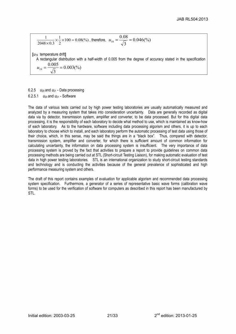
Summary of u18 and u19.

[u18 resolution of digital detector system]

Set the minimum deflection to 30% of the full scale using 12 bit converter:

JAB RL504:2013


(%)08.01002

1

3.02048

1 =×××

, therefore, (%)046.03

08.018 ==u


A rectangular distribution with a half-width of 0.005 from the degree of accuracy stated in the specification

(%)003.03

005.019 ==u

6.2.5 u20 and u21 - Data processing

6.2.5.1 u20 and u21 - Software

The data of various tests carried out by high power testing laboratories are usually automatically measured and analyzed by a measuring system that takes into consideration uncertainty. Data are generally recorded as digital data via by detector, transmission system, amplifier and converter, to be data processed. But for this digital data processing, it is the responsibility of each laboratory to decide what method to use, which is maintained as know-how of each laboratory. As to the hardware, software including data processing algorism and others, it is up to each laboratory to choose which to install, and each laboratory perform the automatic processing of test data using those of their choice, which, in this sense, may be said the things are in a “black box”. Thus, compared with detector, transmission system, amplifier and converter, for which there is sufficient amount of common information for calculating uncertainty, the information on data processing system is insufficient. The very importance of data processing system is proved by the fact that activities to prepare a report to provide guidelines on common data processing methods are being carried out at STL (Short-circuit Testing Liaison), for making automatic evaluation of test data in high power testing laboratories. STL is an international organization to study short-circuit testing standards and technology and is conducting the activities because of the general prevalence of sophisticated and high performance measuring system and others. The draft of this report contains examples of evaluation for applicable algorism and recommended data processing system specification. Furthermore, a generator of a series of representative basic wave forms (calibration wave forms) to be used for the verification of software for computers as described in this report has been manufactured by STL.

JAB RL504:2013


Summary of u18 and u19.

[u20 least-square method] [u21 three(3) crest method]

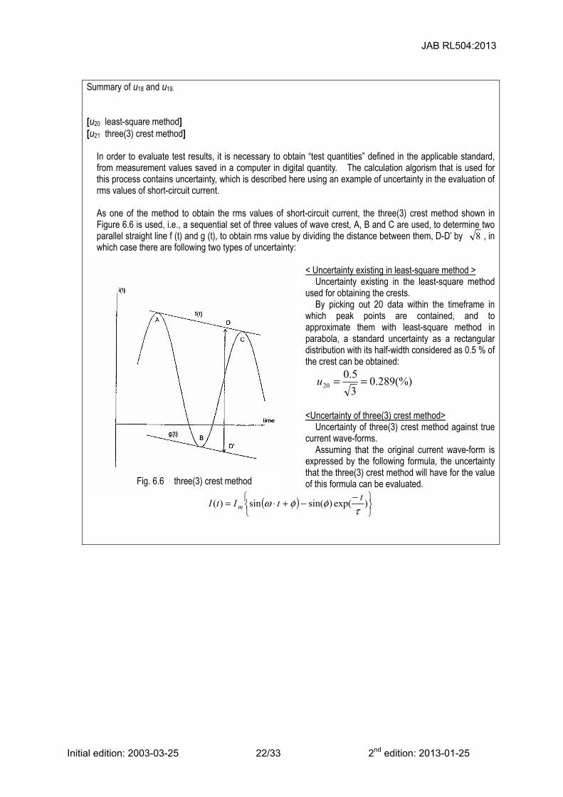
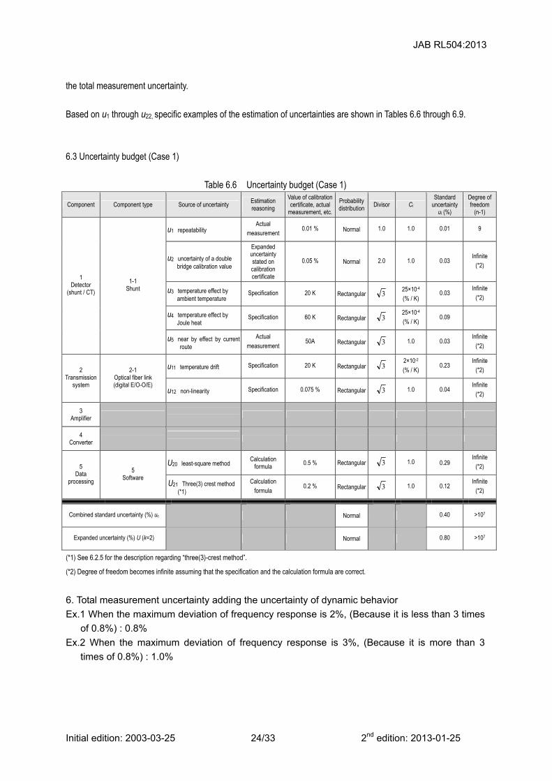
In order to evaluate test results, it is necessary to obtain “test quantities” defined in the applicable standard, from measurement values saved in a computer in digital quantity. The calculation algorism that is used for this process contains uncertainty, which is described here using an example of uncertainty in the evaluation of rms values of short-circuit current.

As one of the method to obtain the rms values of short-circuit current, the three(3) crest method shown in Figure 6.6 is used, i.e., a sequential set of three values of wave crest, A, B and C are used, to determine two parallel straight line f (t) and g (t), to obtain rms value by dividing the distance between them, D-D’ by 8 , in which case there are following two types of uncertainty:

< Uncertainty existing in least-square method >

Uncertainty existing in the least-square method used for obtaining the crests.

By picking out 20 data within the timeframe in which peak points are contained, and to approximate them with least-square method in parabola, a standard uncertainty as a rectangular distribution with its half-width considered as 0.5 % of the crest can be obtained:

(%)289.03

5.020 ==u

<Uncertainty of three(3) crest method>

Uncertainty of three(3) crest method against true current wave-forms.

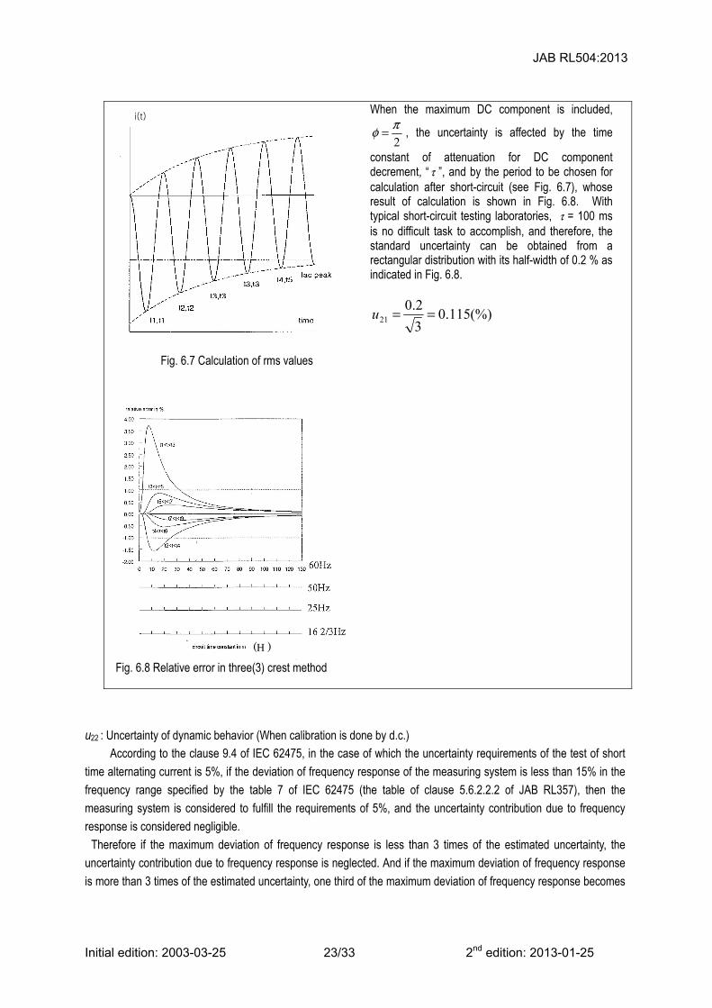
Assuming that the original current wave-form is expressed by the following formula, the uncertainty that the three(3) crest method will have for the value of this formula can be evaluated.

( )

−−+⋅= )exp()sin(sin)(

τφφω ttItI m

Fig. 6.6 three(3) crest method

JAB RL504:2013


i(t)

Fig. 6.7 Calculation of rms values

(τ) Fig. 6.8 Relative error in three(3) crest method

When the maximum DC component is included,

2

πφ = , the uncertainty is affected by the time

constant of attenuation for DC component decrement, “τ ”, and by the period to be chosen for calculation after short-circuit (see Fig. 6.7), whose result of calculation is shown in Fig. 6.8. With typical short-circuit testing laboratories, τ = 100 ms is no difficult task to accomplish, and therefore, the standard uncertainty can be obtained from a rectangular distribution with its half-width of 0.2 % as indicated in Fig. 6.8.

(%)115.03

2.021 ==u

u22 : Uncertainty of dynamic behavior (When calibration is done by d.c.) According to the clause 9.4 of IEC 62475, in the case of which the uncertainty requirements of the test of short

time alternating current is 5%, if the deviation of frequency response of the measuring system is less than 15% in the

frequency range specified by the table 7 of IEC 62475 (the table of clause 5.6.2.2.2 of JAB RL357), then the

measuring system is considered to fulfill the requirements of 5%, and the uncertainty contribution due to frequency

response is considered negligible.

Therefore if the maximum deviation of frequency response is less than 3 times of the estimated uncertainty, the

uncertainty contribution due to frequency response is neglected. And if the maximum deviation of frequency response

is more than 3 times of the estimated uncertainty, one third of the maximum deviation of frequency response becomes

JAB RL504:2013


the total measurement uncertainty.

Based on u1 through u22, specific examples of the estimation of uncertainties are shown in Tables 6.6 through 6.9.

6.3 Uncertainty budget (Case 1)

Table 6.6 Uncertainty budget (Case 1)

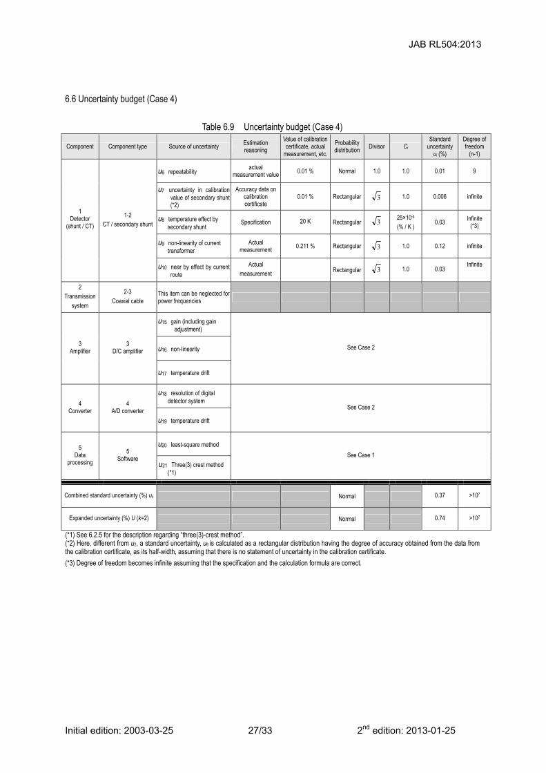
Component Component type Source of uncertainty Estimation reasoning

Value of calibration certificate, actual

measurement, etc.

Probability distribution Divisor Ci

Standard uncertainty

ui (%)

Degree of freedom

(n-1)

u1 repeatability Actual

measurement0.01 % Normal 1.0 1.0 0.01 9

u2 uncertainty of a double bridge calibration value

Expanded uncertainty stated on calibration certificate

0.05 % Normal 2.0 1.0 0.03 Infinite

(*2)

u3 temperature effect by ambient temperature

Specification 20 K Rectangular 3 25×10-4 (% / K)

0.03 Infinite

(*2)

u4 temperature effect by Joule heat

Specification 60 K Rectangular 3 25×10-4 (% / K)

0.09

1 Detector

(shunt / CT)

1-1 Shunt

u5 near by effect by current route

Actual

measurement50A Rectangular 3 1.0 0.03

Infinite

(*2)

u11 temperature drift Specification 20 K Rectangular 3 2×10-2 (% / K)

0.23 Infinite

(*2) 2 Transmission

system

2-1 Optical fiber link (digital E/O-O/E)

u12 non-linearity Specification 0.075 % Rectangular 3 1.0 0.04 Infinite

(*2)

3 Amplifier

4 Converter

U20 least-square method Calculation

formula 0.5 % Rectangular 3 1.0 0.29 Infinite

(*2) 5 Data

processing

5 Software

U21 Three(3) crest method (*1)

Calculation

formula 0.2 % Rectangular 3 1.0 0.12

Infinite

(*2)

Combined standard uncertainty (%) uc Normal 0.40 >107

Expanded uncertainty (%) U (k=2) Normal 0.80 >107

(*1) See 6.2.5 for the description regarding “three(3)-crest method”.

(*2) Degree of freedom becomes infinite assuming that the specification and the calculation formula are correct.

6. Total measurement uncertainty adding the uncertainty of dynamic behavior

Ex.1 When the maximum deviation of frequency response is 2%, (Because it is less than 3 times

of 0.8%) : 0.8%

Ex.2 When the maximum deviation of frequency response is 3%, (Because it is more than 3

times of 0.8%) : 1.0%

JAB RL504:2013






measurement, etc.



ui (%)

Degree of freedom

(n-1)

u1 repeatability




1 Detector

(shunt / CT)

1-1 Shunt


See Case 1

u13 temperature drift Specification 5 K Rectangular 3 1.6×10-1

(% / K) 0.46

Infinite

(*2 2 Transmission

system

2-2 Optical cable

(analogue E/O-O/E) u14 non-linearity Specification 2.0 % Rectangular 3 1.0 1.15

Infinite

(*2

u15 gain (including gain adjustment)

Specification 0.2 % Rectangular 3 1.0 0.12 Infinite

(*2

u16 non-linearity Specification 0.05 % Rectangular 3 1.0 0.03 Infinite

(*2 3

Amplifier 3

D/C amplifier

u17 temperature drift Specification 5 K Rectangular 3 3×10-2 (% / K)

0.09 Infinite

(*2

u18 resolution of digital detector system

Specification 0.08 % Rectangular 3 1.0 0.05 Infinite

(*2 4 Converter

4 A/D converter

u19 temperature drift Specification 0.005 % Rectangular 3 1.0 0.003 Infinite

(*2

u20 least-square method 5 Data

processing

5 Software

u21 Three(3) crest method (*1)

See Case 1







of 2.6%) : 2.6%


times of 2.6%) : 3%

JAB RL504:2013






measurement, etc.



ui (%)

Degree of freedom

(n-1)

u1 repeatability




1 Detector

(shunt / CT)

1-1 Shunt


See Case 1

2

Transmission system

2-3

Coaxial cable This item can be neglected for commercial frequencies.


u16 non-linearity 3

Amplifier 3

D/C amplifier

u17 temperature drift

See Case 2

u18 resolution of digital detector system 4

Converter 4

A/D converter


See Case 2


processing

5 Software


See Case 1






of 0.74%) : 0.74%


times of 0.74%) : 1.0%

JAB RL504:2013






measurement, etc.



ui (%)

Degree of freedom

(n-1)

u6 repeatability actual

measurement value 0.01 % Normal 1.0 1.0 0.01 9

u7 uncertainty in calibration value of secondary shunt (*2)

Accuracy data on calibration certificate

0.01 % Rectangular 3 1.0 0.006 infinite

u8 temperature effect by secondary shunt

Specification 20 K Rectangular 3 25×10-4 (% / K )

0.03 Infinite (*3)

u9 non-linearity of current transformer

Actual measurement 0.211 % Rectangular 3 1.0 0.12 infinite

1 Detector

(shunt / CT)

1-2 CT / secondary shunt


Actual

measurement Rectangular 3 1.0 0.03

Infinite

2 Transmission

system

2-3 Coaxial cable

This item can be neglected for power frequencies


u16 non-linearity 3

Amplifier 3

D/C amplifier


See Case 2

u18 resolution of digital detector system 4

Converter 4

A/D converter


See Case 2


processing

5 Software


See Case 1



(*1) See 6.2.5 for the description regarding “three(3)-crest method”. (*2) Here, different from u2, a standard uncertainty, u6 is calculated as a rectangular distribution having the degree of accuracy obtained from the data from the calibration certificate, as its half-width, assuming that there is no statement of uncertainty in the calibration certificate.


JAB RL504:2013


7. CLOSURE

This is the summary of the results of studies made by the High Power Technical Sub-committee on specific examples

of the estimation of uncertainty necessary for a high power testing laboratory aiming to meet the requirements of

ISO/IEC 17025.

JAB NOTE4 is wished to be improved by receiving valuable advice from relevant industries and specialists as well as

the accumulation of assessment experiences.

- Members of the Preparation of JAB NOTE4 –(At the date of issue)

High Power Technical Sub-committee/ JAB Laboratory Technical Committee

NAME AFFILIATION

(Chair) Kunio HIRASAWA Hitachi, Ltd.

(Member) Hiromi ISHII Nissin Electric Co., Ltd.

Hiroshi INOUE The Japan Electrical Manufacturers' Association

Yasukuni KUZUMA Central Research Institute of Electric Power Industry

Masaya SAKAMOTO TOSHIBA Corporation

Tatsuo SAWADA Mitsubishi Electric Corporation

Masatoshi NAKAJIMA FUJI ELECTRIC CO., LTD.

Shigeo NONAKA System-Science Research Laboratory

Eiichi Haginomori Ex-Kyushu Institute of Technology

Yoshihiko Matsui Meiden T&D Corporation.

(Secretariat) Koichi SAZANAMI Japan Accreditation Board

JAB RL504:2013


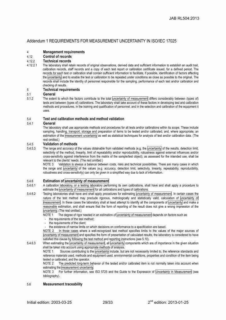
Addendum 1 REQUIREMENTS FOR MEASUREMENT UNCERTAINTY IN ISO/IEC 17025

4 Management requirements 4.12 Control of records 4.12.2 Technical records 4.12.2.1 The laboratory shall retain records of original observations, derived data and sufficient information to establish an audit trail,

calibration records, staff records and a copy of each test report or calibration certificate issued, for a defined period. The records for each test or calibration shall contain sufficient information to facilitate, if possible, identification of factors affecting the uncertainty and to enable the test or calibration to be repeated under conditions as close as possible to the original. The records shall include the identity of personnel responsible for the sampling, performance of each test and/or calibration and checking of results.

5 Technical requirements 5.1 General 5.1.2 The extent to which the factors contribute to the total uncertainty of measurement differs considerably between (types of)

tests and between (types of) calibrations. The laboratory shall take account of these factors in developing test and calibration methods and procedures, in the training and qualification of personnel, and in the selection and calibration of the equipment it uses.

5.4 Test and calibration methods and method validation 5.4.1 General

The laboratory shall use appropriate methods and procedures for all tests and/or calibrations within its scope. These include sampling, handling, transport, storage and preparation of items to be tested and/or calibrated, and, where appropriate, an estimation of the measurement uncertainty as well as statistical techniques for analysis of test and/or calibration data. (The rest omitted.)

5.4.5 Validation of methods 5.4.5.3 The range and accuracy of the values obtainable from validated methods (e.g. the uncertainty of the results, detection limit,

selectivity of the method, linearity, limit of repeatability and/or reproducibility, robustness against external influences and/or cross-sensitivity against interference from the matrix of the sample/test object), as assessed for the intended use, shall be relevant to the clients' needs. (The rest omitted.) NOTE 3 Validation is always a balance between costs, risks and technical possibilities. There are many cases in which the range and uncertainty of the values (e.g. accuracy, detection limit, selectivity, linearity, repeatability, reproducibility, robustness and cross-sensitivity) can only be given in a simplified way due to lack of information.

5.4.6 Estimation of uncertainty of measurement 5.4.6.1 A calibration laboratory, or a testing laboratory performing its own calibrations, shall have and shall apply a procedure to

estimate the uncertainty of measurement for all calibrations and types of calibrations. 5.4.6.2 Testing laboratories shall have and shall apply procedures for estimating uncertainty of measurement. In certain cases the

nature of the test method may preclude rigorous, metrologically and statistically valid, calculation of uncertainty of measurement. In these cases the laboratory shall at least attempt to identify all the components of uncertainty and make a reasonable estimation, and shall ensure that the form of reporting of the result does not give a wrong impression of the uncertainty. (The rest omitted.) NOTE 1 The degree of rigor needed in an estimation of uncertainty of measurement depends on factors such as: - the requirements of the test method; - the requirements of the client; - the existence of narrow limits on which decisions on conformance to a specification are based. NOTE 2 In those cases where a well-recognized test method specifies limits to the values of the major sources of uncertainty of measurement and specifies the form of presentation of calculated results, the laboratory is considered to have satisfied this clause by following the test method and reporting instructions (see 5.10).

5.4.6.3 When estimating the uncertainty of measurement, all uncertainty components which are of importance in the given situation shall be taken into account using appropriate methods of analysis. NOTE 1 Sources contributing to the uncertainty include, but are not necessarily limited to, the reference standards and reference materials used, methods and equipment used, environmental conditions, properties and condition of the item being tested or calibrated, and the operator. NOTE 2 The predicted long-term behavior of the tested and/or calibrated item is not normally taken into account when estimating the measurement uncertainty. NOTE 3 For further information, see ISO 5725 and the Guide to the Expression of Uncertainty in Measurement (see bibliography).

5.6 Measurement traceability

JAB RL504:2013


5.6.2 Specific requirements 5.6.2.1 Calibration 5.6.2.1.1 (Omitted) A calibration laboratory establishes traceability of its own measurement standards and measuring instruments to

the SI by means of an unbroken chain of calibrations or comparisons linking them to relevant primary standards of the SI units of measurement. The link to SI units may be achieved by reference to national measurement standards. National measurement standards may be primary standards, which are primary realizations of the SI units or agreed representations of SI units based on fundamental physical constants, or they may be secondary standards which are standards calibrated by another national metrology institute. When using external calibration services, traceability of measurement shall be assured by the use of calibration services from laboratories that can demonstrate competence, measurement capability and traceability. The calibration certificates issued by these laboratories shall contain the measurement results, including the measurement uncertainty and/or a statement of compliance with an identified metrological specification (see also 5.10.4.2).

5.6.2.2 Testing 5.6.2.2.1 For testing laboratories, the requirements given in 5.6.2.1 apply for measuring and test equipment with measuring functions

used, unless it has been established that the associated contribution from the calibration contributes little to the total uncertainty of the test result. When this situation arises, the laboratory shall ensure that the equipment used can provide the uncertainty of measurement needed. NOTE The extent to which the requirements in 5.6.2.1 should be followed depends on the relative contribution of the calibration uncertainty to the total uncertainty. If calibration is the dominant factor, the requirements should be strictly followed.

5.10 Reporting the results 5.10.3 Test reports 5.10.3.1 c) where applicable, a statement on the estimated uncertainty of measurement; information on uncertainty is needed in test

reports when it is relevant to the validity or application of the test results, when a client's instruction so requires, or when the uncertainty affects compliance to a specification limit;

5.10.4 Calibration certificate 5.10.4.1b) the uncertainty of measurement and/or a statement of compliance with an identified metrological specification or clauses

thereof; 5.10.4.2 The calibration certificate shall relate only to quantities and the results of functional tests. If a statement of compliance with a

specification is made, this shall identify which clauses of the specification are met or not met. When a statement of compliance with a specification, is made omitting the measurement results and associated uncertainties, the laboratory shall record those results and maintain them for possible future reference. When statements of compliance are made, the uncertainty of measurement shall be taken into account.

JAB RL504:2013


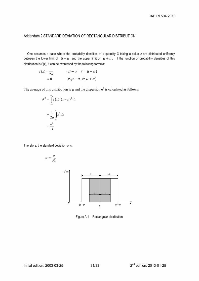
Addendum 2 STANDARD DEVIATION OF RECTANGULAR DISTRIBUTION

One assumes a case where the probability densities of a quantity X taking a value x are distributed uniformly between the lower limit of a−μ and the upper limit of a+μ . If the function of probability densities of this

distribution is f (x), it can be expressed by the following formula:

a

xf2

1)( = ( a−μ ≦x≦ a+μ )

0= (x< a−μ , x> a+μ )

The average of this distribution is μ and the dispersion σ2 is calculated as follows:

∞

∞−

−⋅= dxxxf 22 )()( μσ

3

2

1

2

2

a

dxxa

a

a

=

= −

Therefore, the standard deviation σ is:

3

a=σ

Figure A.1 Rectangular distribution

JAB RL504:2013


Form No. JAB NF18 REV.0

HISTORY OF REVISIONS

Edition No.

Outline of Revision Issue Date Document

Owner Approved

by

1 Document issued 2003-03-25 Laboratory Technical Committee

2 Review of adding uncertainty of dynamic behavior

2113-01-25 Program Manager (Electrical Testing)

Laboratory Technical Committee

JAB RL504:2013


JAPAN ACCREDITATION BOARD Gotanda AN Bldg. 3rd floor

22-1, Higashi Gotanda 1-chome, Shinagawa-ku Tokyo 141-0022, JAPAN

Phone: +81-3-3442-1217 Fax: +81-3-5475-2780

The reproduction, reprinting, etc. of this document without authorization is prohibited by

copyright law.

Date post:	19-Jul-2018
Category:	Documents
Upload:	truongliem
View:	254 times
Download:	2 times

ESTIMATION OF MEASUREMENT UNCERTAINTY (Electrical … · ESTIMATION OF MEASUREMENT UNCERTAINTY...

Documents