LUND UNIVERSITY

PO Box 117221 00 Lund+46 46-222 00 00

Estimation of Spherical Wave Coefficients from 3D Positioner Channel Measurements

Bernland, Anders; Gustafsson, Mats; Gustafson, Carl; Tufvesson, Fredrik

2012

Link to publication

Citation for published version (APA):Bernland, A., Gustafsson, M., Gustafson, C., & Tufvesson, F. (2012). Estimation of Spherical Wave Coefficientsfrom 3D Positioner Channel Measurements. (Technical Report LUTEDX/(TEAT-7215)/1-11/(2012); Vol. TEAT-7215). [Publisher information missing].

Total number of authors:4

General rightsUnless other specific re-use rights are stated the following general rights apply:Copyright and moral rights for the publications made accessible in the public portal are retained by the authorsand/or other copyright owners and it is a condition of accessing publications that users recognise and abide by thelegal requirements associated with these rights. • Users may download and print one copy of any publication from the public portal for the purpose of private studyor research. • You may not further distribute the material or use it for any profit-making activity or commercial gain • You may freely distribute the URL identifying the publication in the public portal

Read more about Creative commons licenses: https://creativecommons.org/licenses/Take down policyIf you believe that this document breaches copyright please contact us providing details, and we will removeaccess to the work immediately and investigate your claim.

Download date: 14. Jan. 2022

Electromagnetic TheoryDepartment of Electrical and Information TechnologyLund UniversitySweden

CODEN:LUTEDX/(TEAT-7215)/1-11/(2012)

Estimation of Spherical WaveCoefficients from 3D PositionerChannel Measurements

Anders Bernland, Mats Gustafsson, Carl Gustafson,and Fredrik Tufvesson

Anders Bernland, Mats Gustafsson, Carl Gustafson, and Fredrik Tufvesson{Anders.Bernland,Mats.Gustafsson, Carl.Gustafson,Fredrik.Tufvesson}@eit.lth.se

Department of Electrical and Information TechnologyElectromagnetic TheoryLund UniversityP.O. Box 118SE-221 00 LundSweden

Editor: Gerhard Kristenssonc© Anders Bernland et al., Lund, March 5, 2012

1

Abstract

Electromagnetic vector spherical waves have been used recently to model an-

tenna channel interaction and the available degrees of freedom in MIMO sys-

tems. However, there are no previous accounts of a method to estimate spher-

ical wave coe�cients from channel measurements. One approach, using a

3D positioner, is presented in this letter, both in theory and practice. Mea-

surement results are presented and discussed. One conclusion is that using

randomly positioned measurements within a volume is less sensitive to noise

than using only measurements on the surface.

1 Introduction

Real-world measurements and theoretical modelling of antennas and propagationchannels are crucial to wireless communication, and have been the focus of extensiveresearch for many years [10]. One way to the increase the capacity in wireless systemsis to use multiple-input multiple-output (MIMO) technology. MIMO requires severaldegrees of freedom, and the degrees of freedom depend both on the mutual couplingbetween antenna elements and the richness of the channel. It is therefore desirable toseparate the antenna and channel in�uence. One approach to do this is the double-directional channel model, which describes the channel in terms of plane waves, ormulti-path components [7, 10].

Electromagnetic vector spherical waves provide a compact description of a single-or multi-port antenna in terms of the antenna scattering matrix, which describesthe antenna receiving, transmitting and scattering properties [4]. One bene�t isthat only a few terms are needed for a small antenna. Furthermore, spherical wavesare used within spherical near-�eld antenna measurements, where they enable thenecessary probe corrections and near-�eld to far-�eld transforms [4, 8].

Spherical vector wave approaches to theoretically model antenna channel inter-action and the available degrees of freedom have been given in [2, 3, 9], separatingthe antenna from the channel in a compact and intuitive way. It is well knownthat a small antenna only can excite a limited number of spherical waves [1], whichrestricts the available degrees of freedom for a small multi-port antenna. It is not,however well-known how many degrees of freedom a given propagation channel cansupport. Furthermore, to the authors best knowledge there are no previous publi-cations where spherical waves are estimated from channel measurements, althoughsome preliminary studies have been done [6].

The main objective of this letter is to present a method to estimate sphericalwave coe�cients from channel measurements. For this, a 3D positioner is used tomove the receiving antenna to di�erent positions and orientations within a cube, andprobe correction [4] is used to separate the in�uence of the receiving antenna. Thewhole volume of the cube as well as di�erent subsets are used in separate estimationsto determine how the measurements points should be positioned.

2

2 Preliminaries

In a source-free region enclosed by spherical surfaces, the electric �eld can be writtenas a sum of regular (v) and outgoing (u(1)) vector spherical waves (time conventione−iωt):

E(r, k) = k√η0∑ν

d(1)ν u(1)ν (kr) + d(2)ν vν(kr). (2.1)

Here the free space parameters are wavenumber k = ω/c, speed of light c andimpedance η0. The spatial coordinate is denoted r, with r = |r| and r = r/r. Thespherical waves are de�ned as in the book [4] by Hansen, but with slightly di�erentnotation (see Appendix A). The multi-index ν = 2(l2 + l− 1 +m) + τ is introducedin place of the indices {τ,m, l}, where τ = 1 (odd ν) corresponds to a magnetic2l-pole (TEl-mode), while τ = 2 (even ν) identi�es an electric 2l-pole (TMl-mode).The basis function in the azimuth angle φ is eimφ.

The antenna source scattering matrix completely describes the antenna proper-ties: (

Γ R′

T′ S′

)(w(2)

d(2)

)=

(w(1)

d(1)

). (2.2)

Here d(2) = (d(2)1 d

(2)2 . . . )T and w(2) are the coe�cients of the incident regular waves

and transmitted signal, whereas d(1) and w(1) are the coe�cients of the scatteredor transmitted outgoing waves and received signal. The transmitted and receivedsignals are vectors in the case of a multi-port antenna. The primes are included hereto indicate that the source scattering matrix formulation in (2.163) in [4] is used.The transmitting coe�cients T ′ν and receiving coe�cients R′ν are included in T′ andR′, respectively [4].

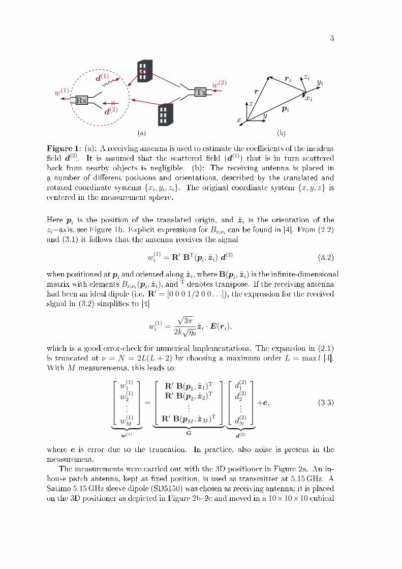
The main purpose of this letter is to determine the spherical wave coe�cientsd(2)ν from channel measurements. More precisely, consider a transmitting antenna ina propagation channel, as in Figure 1a. Within any sphere containing no scatterers,only the regular waves contribute to the sum in (2.1). The coe�cients d

(2)ν will

be estimated from measurements with the receiving antenna placed in a number ofdi�erent positions and orientations. It is assumed that the scattered �eld that is inturn scattered back from nearby objects is negligible.

3 Method

In order to estimate the spherical wave coe�cients, the receiving antenna is placedin a number of di�erent positions and orientations. When the antenna is placedin the origin in its original orientation, it receives the signal w(1) given by (2.2).When it is moved and/or rotated, expressions for w(1) are derived by expressing thespherical waves in the original coordinate system {x, y, z} as sums over the sphericalwaves in the translated and rotated coordinate system {xi, yi, zi}:

vν(kr) =∑νi

Bν,νi(pi, zi)vνi(kri). (3.1)

3

(a) (b)

Figure 1: (a): A receiving antenna is used to estimate the coe�cients of the incident�eld d(2). It is assumed that the scattered �eld (d(1)) that is in turn scatteredback from nearby objects is negligible. (b): The receiving antenna is placed ina number of di�erent positions and orientations, described by the translated androtated coordinate systems {xi, yi, zi}. The original coordinate system {x, y, z} iscentered in the measurement sphere.

Here pi is the position of the translated origin, and zi is the orientation of thezi−axis, see Figure 1b. Explicit expressions for Bν,νi can be found in [4]. From (2.2)and (3.1) it follows that the antenna receives the signal

w(1)i = R′ BT(pi, zi) d(2) (3.2)

when positioned at pi and oriented along zi, whereB(pi, zi) is the in�nite-dimensionalmatrix with elements Bν,νi(pi, zi), and

T denotes transpose. If the receiving antennahad been an ideal dipole (i.e. R′ = [0 0 0 1/2 0 0 . . .]), the expression for the receivedsignal in (3.2) simpli�es to [4]

w(1)i =

√3π

2k√η0zi ·E(ri),

which is a good error-check for numerical implementations. The expansion in (2.1)is truncated at ν = N = 2L(L + 2) by choosing a maximum order L = max l [4].With M measurements, this leads to:

w(1)1

w(1)2...

w(1)M

︸ ︷︷ ︸

w(1)

=

R′ B(p1, z1)

T

R′ B(p2, z2)T

...R′ B(pM , zM)T

︸ ︷︷ ︸

G

d(2)1

d(2)2...

d(2)N

︸ ︷︷ ︸

d(2)

+e, (3.3)

where e is error due to the truncation. In practice, also noise is present in themeasurement.

The measurements were carried out with the 3D positioner in Figure 2a. An in-house patch antenna, kept at �xed position, is used as transmitter at 5.15 GHz. ASatimo 5.15 GHz sleeve dipole (SD5150) was chosen as receiving antenna; it is placedon the 3D positioner as depicted in Figure 2b�2c and moved in a 10×10×10 cubical

4

(a)

(b)

(c)

(d)

Figure 2: (a): The 3D positioner used in the measurements. (b)�(c): The Satimo5.15 GHz sleeve dipole used as receiving antenna to estimate coe�cients, mounted in(b): z-polarization and (c): x-polarization. The 3D positioner rotates the antennain x−polarization 90◦ to measure y−polarization. (d): The Skycross UWB antennaused for validation.

grid with stepsize 15mm (≈ 0.26λ), measuring x, y, and z polarization at each pointfor a total of 3000 measurements. Here the coordinates given to the 3D positionermust �rst be corrected for the o�set in phase center as the antenna is rotated. Thetransmitting and receiving antennas are connected to port 1 and 2 of an AgilentE8361A vector network analyzer, which was calibrated and used to measure thetransfer function S21 = w

(1)Rx/w

(2)Tx . An ampli�er was used at the transmitter side.

For later use as validation of the estimated coe�cients, the Skycross UWB antenna(SMT-2TO6MB-A) in Figure 2d (frequency range 2.3-5.9GHz) is used as receivingantenna in place of the sleeve dipole in otherwise identical measurements; it is movedalong a subset of the points in the cubical grid for a total of 90 measurements.

For veri�cation purposes, data has also been simulated: 100 random plane waveswith independent polarization, complex Gaussian amplitude and angles of arrivaluniformly distributed over the sphere, distorted by zero mean white Gaussian noise.In this case, closed form expressions of the coe�cients in d(2) are known [4], whichmakes it possible to check the accuracy of the method as a function of SNR.

The matrix G in (3.3) is determined with in-house Matlab-scripts, using the po-sitions pi and orientations zi from the 3D positioner and the receiving coe�cientsR′ν of the antennas. For this reason, both the sleeve dipole and UWB antenna havebeen characterized in a Satimo Stargate-24 chamber where the antenna transmit-ting coe�cients T ′ν are given as output. The receiving coe�cients R′ν are given byR′{τ,m,l} = (−1)mT ′{τ,−m,l}/2 [4]. The sleeve dipole is very close to a Hertzian dipole,

5

and the higher orders contribute little to the results of the 3D positioner mea-surements. It is observed that the smallest errors are obtained when the receivingcoe�cients R′ν are truncated to contain only the dipole term.

An estimate d(2)

of the unknown coe�cients in d(2) can be computed from thesystem of equations in (3.3). A �rst approach is the least-squares solution

d(2)LSQ = arg min

d(2)||Gd(2) −w(1)||2,

but the singular values of G suggest that this is an ill-posed problem. Furthermore,when computing least-squares solutions from simulated data, it is seen that largeerrors are introduced for the coe�cients of high orders l. Therefore, a more elaboratemethod should be used. Here, a regularized solution by means of Tikhonov's methodis chosen [5]:

d(2)

= arg mind(2)

(||Gd(2) −w(1)||2 + ||λregd(2)||2

).

The regularization parameter λreg is determined with the L-curve criterion [5]. Theregularization works well when tested on simulated data, and seem to work also for

measured data. It is also seen that the estimated coe�cients d(2)

are independentof the truncation order L, as long as it is chosen large enough. A rule of thumb isL > krcirc ≈ 12.6, where rcirc is the radius of the smallest sphere circumscribing thecube.

The measurement problem considered here show some similarities with near-�eld antenna measurements, see e.g. [4, 8, 11]. However, none of these methods aredirectly applicable here.

4 Results and Discussion

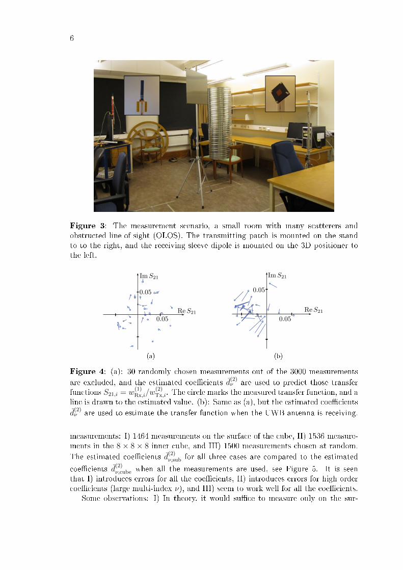
The measurement scenario is a small room with many scatterers and obstructed-line-of-sight (OLOS), see Figure 3. It is chosen to get a rich channel, and a challengingproblem to estimate the spherical wave coe�cients. Measurements were also carriedout in a large, empty room under line-of-sight conditions, with similar results.

The spherical wave coe�cients d(2)ν are estimated from the measured data as

described above. For a �rst validation, 30 randomly chosen measurements out of the3000 measurements are excluded from the estimation, and the estimated coe�cientsd(2)ν are used to predict those transfer functions S21,i = w

(1)Rx,i/w

(2)Tx,i. The results can

be found in Figure 4a. In the second validation, the same estimates d(2)ν are used

to estimate the transfer function for the UWB antenna, see Figure 4b. The errorsare slightly larger here; at 5.15 GHz the UWB antenna has a complicated radiationpattern, and small errors in positioning and in�uence from nearby objects give largeerrors for the received signal. However, the results in Figure 4 indicate that thespherical wave coe�cients have been estimated with acceptable errors.

To investigate if, and how, the number of measurements can be reduced, thespherical wave coe�cients are estimated using three di�erent subsets of the 3000

6

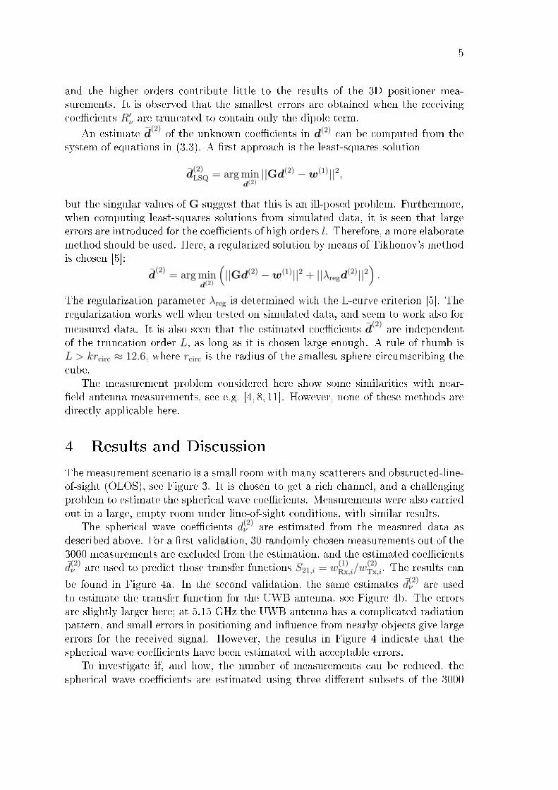
Figure 3: The measurement scenario, a small room with many scatterers andobstructed-line-of-sight (OLOS). The transmitting patch is mounted on the standto to the right, and the receiving sleeve dipole is mounted on the 3D positioner tothe left.

(a) (b)

Figure 4: (a): 30 randomly chosen measurements out of the 3000 measurements

are excluded, and the estimated coe�cients d(2)ν are used to predict those transfer

functions S21,i = w(1)Rx,i/w

(2)Tx,i. The circle marks the measured transfer function, and a

line is drawn to the estimated value. (b): Same as (a), but the estimated coe�cients

d(2)ν are used to estimate the transfer function when the UWB antenna is receiving.

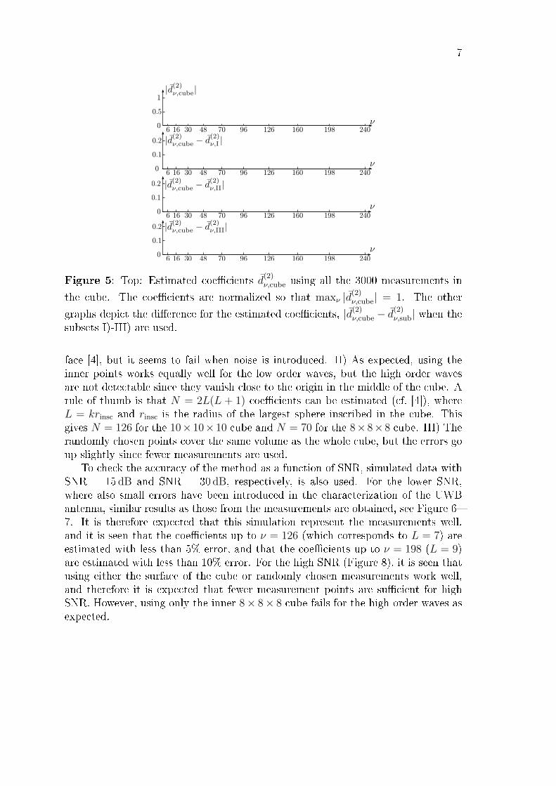
measurements: I) 1464 measurements on the surface of the cube, II) 1536 measure-ments in the 8 × 8 × 8 inner cube, and III) 1500 measurements chosen at random.

The estimated coe�cients d(2)ν,sub for all three cases are compared to the estimated

coe�cients d(2)ν,cube when all the measurements are used, see Figure 5. It is seen

that I) introduces errors for all the coe�cients, II) introduces errors for high ordercoe�cients (large multi-index ν), and III) seem to work well for all the coe�cients.

Some observations: I) In theory, it would su�ce to measure only on the sur-

7

6 16 30 48 70 96 126 160 198 2400

0.5

1

6 16 30 48 70 96 126 160 198 2400

0.1

0.2

0

0.1

0.2

6 16 30 48 70 96 126 160 198 2400

0.1

0.2

6 16 30 48 70 96 126 160 198 240

Figure 5: Top: Estimated coe�cients d(2)ν,cube using all the 3000 measurements in

the cube. The coe�cients are normalized so that maxν |d(2)ν,cube| = 1. The other

graphs depict the di�erence for the estimated coe�cients, |d(2)ν,cube − d(2)ν,sub| when the

subsets I)-III) are used.

face [4], but it seems to fail when noise is introduced. II) As expected, using theinner points works equally well for the low order waves, but the high order wavesare not detectable since they vanish close to the origin in the middle of the cube. Arule of thumb is that N = 2L(L + 1) coe�cients can be estimated (cf. [4]), whereL = krinsc and rinsc is the radius of the largest sphere inscribed in the cube. Thisgives N = 126 for the 10×10×10 cube and N = 70 for the 8×8×8 cube. III) Therandomly chosen points cover the same volume as the whole cube, but the errors goup slightly since fewer measurements are used.

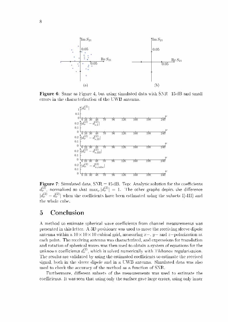
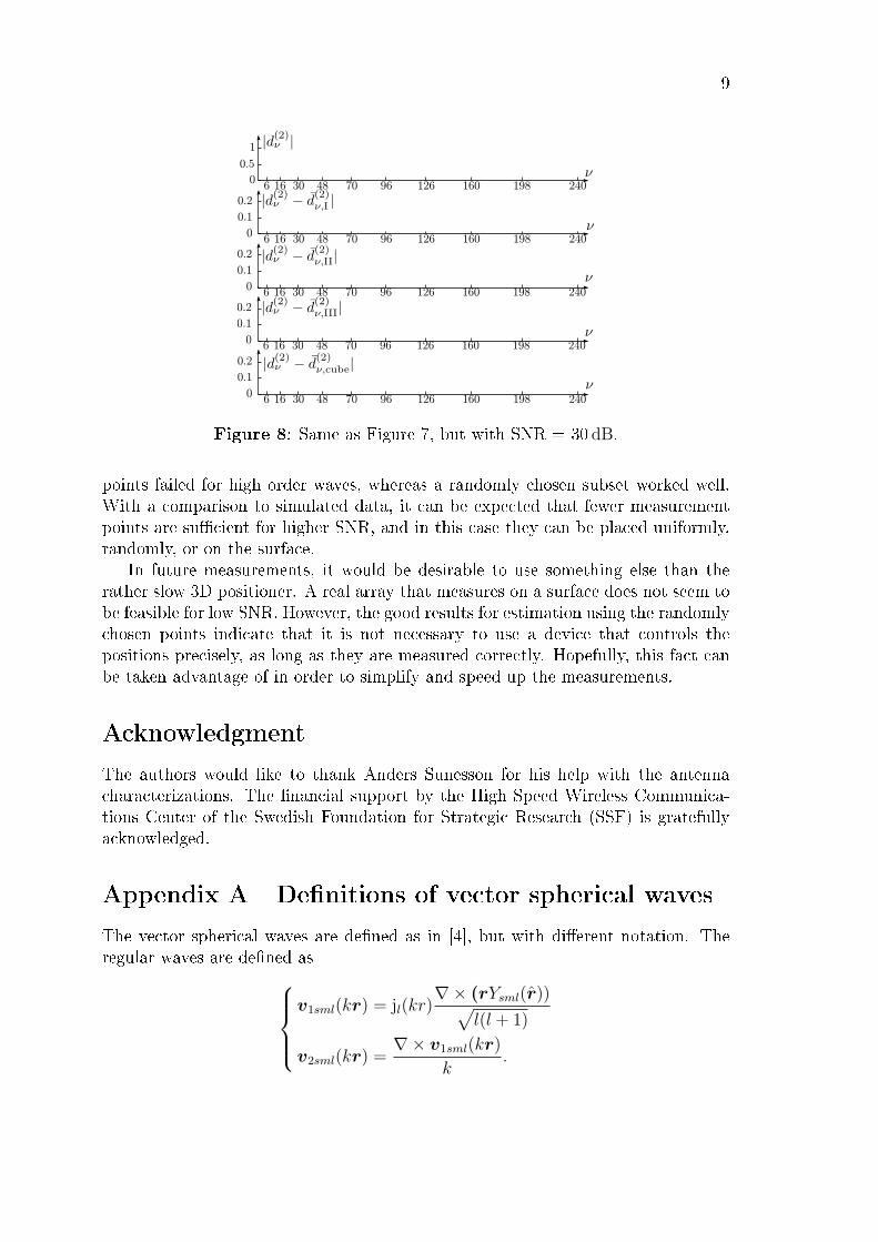
To check the accuracy of the method as a function of SNR, simulated data withSNR = 15 dB and SNR = 30 dB, respectively, is also used. For the lower SNR,where also small errors have been introduced in the characterization of the UWBantenna, similar results as those from the measurements are obtained, see Figure 6�7. It is therefore expected that this simulation represent the measurements well,and it is seen that the coe�cients up to ν = 126 (which corresponds to L = 7) areestimated with less than 5% error, and that the coe�cients up to ν = 198 (L = 9)are estimated with less than 10% error. For the high SNR (Figure 8), it is seen thatusing either the surface of the cube or randomly chosen measurements work well,and therefore it is expected that fewer measurement points are su�cient for highSNR. However, using only the inner 8× 8× 8 cube fails for the high order waves asexpected.

8

(a) (b)

Figure 6: Same as Figure 4, but using simulated data with SNR=15 dB and smallerrors in the characterization of the UWB antenna.

6 16 30 48 70 96 126 160 198 2400

0.5

1

0

0.1

0.2

6 16 30 48 70 96 126 160 198 240

0

0.1

0.2

6 16 30 48 70 96 126 160 198 240

0

0.1

0.2

6 16 30 48 70 96 126 160 198 240

0

0.1

0.2

6 16 30 48 70 96 126 160 198 240

Figure 7: Simulated data, SNR = 15 dB. Top: Analytic solution for the coe�cientsd(2)ν , normalized so that maxν |d(2)ν | = 1. The other graphs depict the di�erence

|d(2)ν − d(2)ν | when the coe�cients have been estimated using the subsets I)-III) andthe whole cube.

5 Conclusion

A method to estimate spherical wave coe�cients from channel measurements waspresented in this letter. A 3D positioner was used to move the receiving sleeve dipoleantenna within a 10×10×10 cubical grid, measuring x−, y− and z−polarization ateach point. The receiving antenna was characterized, and expressions for translationand rotation of spherical waves was then used to obtain a system of equations for theunknown coe�cients d

(2)ν , which is solved numerically with Tikhonov regularization.

The results are validated by using the estimated coe�cients to estimate the receivedsignal, both in the sleeve dipole and in a UWB antenna. Simulated data was alsoused to check the accuracy of the method as a function of SNR.

Furthermore, di�erent subsets of the measurements was used to estimate thecoe�cients. It was seen that using only the surface gave large errors, using only inner

9

6 16 30 48 70 96 126 160 198 2400

0.5

1

0

0.1

0.2

6 16 30 48 70 96 126 160 198 240

0

0.1

0.2

6 16 30 48 70 96 126 160 198 240

0

0.1

0.2

6 16 30 48 70 96 126 160 198 240

0

0.1

0.2

6 16 30 48 70 96 126 160 198 240

Figure 8: Same as Figure 7, but with SNR = 30 dB.

points failed for high order waves, whereas a randomly chosen subset worked well.With a comparison to simulated data, it can be expected that fewer measurementpoints are su�cient for higher SNR, and in this case they can be placed uniformly,randomly, or on the surface.

In future measurements, it would be desirable to use something else than therather slow 3D positioner. A real array that measures on a surface does not seem tobe feasible for low SNR. However, the good results for estimation using the randomlychosen points indicate that it is not necessary to use a device that controls thepositions precisely, as long as they are measured correctly. Hopefully, this fact canbe taken advantage of in order to simplify and speed up the measurements.

Acknowledgment

The authors would like to thank Anders Sunesson for his help with the antennacharacterizations. The �nancial support by the High Speed Wireless Communica-tions Center of the Swedish Foundation for Strategic Research (SSF) is gratefullyacknowledged.

Appendix A De�nitions of vector spherical waves

The vector spherical waves are de�ned as in [4], but with di�erent notation. Theregular waves are de�ned as

v1sml(kr) = jl(kr)∇× (rYsml(r))√

l(l + 1)

v2sml(kr) =∇× v1sml(kr)

k.

10

Here jl denotes the spherical Bessel function of order l [4]. The Bessel function isreplaced with a spherical Hankel function of the �rst kind to get outgoing vectorspherical waves u

(1)τsml. The spherical harmonics Ysml are given by

Ysml(θ, φ) = (−1)m

√(2l + 1)

4π

(l −m)!

(l +m)!Pml (cos θ)eimφ,

where Pml are associated Legendre polynomials [4]. The polar angle is denoted

θ while φ is the azimuth angle. The range of the indices are l = 1, 2, . . . andm = −l,−l + 1, . . . l.

References

[1] A. Bernland. Bandwidth limitations for scattering of higher order electro-magnetic spherical waves with implications for the antenna scattering matrix.Technical Report LUTEDX/(TEAT-7214)/1-23/(2011), Lund University, De-partment of Electrical and Information Technology, P.O. Box 118, S-221 00Lund, Sweden, 2011. http://www.eit.lth.se.

[2] A. A. Glazunov, M. Gustafsson, A. Molisch, and F. Tufvesson. Physical mod-eling of multiple-input multiple-output antennas and channels by means of thespherical vector wave expansion. IET Microwaves, Antennas & Propagation,4(6), 778�791, 2010.

[3] A. A. Glazunov, M. Gustafsson, A. Molisch, F. Tufvesson, and G. Kristensson.Spherical vector wave expansion of gaussian electromagnetic �elds for antenna-channel interaction analysis. IEEE Trans. Antennas Propagat., 3(2), 214�227,2009.

[4] J. E. Hansen, editor. Spherical Near-Field Antenna Measurements. Number 26in IEE electromagnetic waves series. Peter Peregrinus Ltd., Stevenage, UK,1988. ISBN: 0-86341-110-X.

[5] P. C. Hansen. Regularization tools version 4.0 for Matlab 7.3. NumericalAlgorithms, 46, 189�194, 2007.

[6] A. Khatun, T. Laitinen, and P. Vainikainen. Noise sensitivity analysis of spher-ical wave modelling of radio channels using linear scanners. In Microwave Con-ference Proceedings (APMC), 2010 Asia-Paci�c, pages 2119�2122, Yokohama,December 2010.

[7] V.-M. Kolmonen, P. Almers, J. Salmi, J. Koivunen, K. Haneda, A. Richter,F. Tufvesson, A. Molisch, and P. Vainikainen. A dynamic dual-link widebandMIMO channel sounder for 5.3 GHz. IEEE Trans. Instrumentation and Mea-surement, 59(4), 873�883, April 2010.

11

[8] T. Laitinen, S. Pivnenko, J. M. Nielsen, and O. Breinbjerg. Theory and practiceof the FFT/matrix inversion technique for probe-corrected spherical near-�eldantenna measurements with high-order probes. IEEE Trans. Antennas Propa-gat., 58(8), 2623�2631, August 2010.

[9] M. D. Migliore. An intuitive electromagnetic approach to MIMO communica-tion systems. IEEE Trans. Antennas Propagat., 48(3), 128�137, June 2006.

[10] A. F. Molisch. Wireless Communications. John Wiley & Sons, New York,second edition, 2011.

[11] C. H. Schmidt, M. M. Leibfritz, and T. F. Eibert. Fully probe-correctednear-�eld far-�eld transformation employing plane wave expansion and diag-onal translation operators. IEEE Trans. Antennas Propagat., 56(3), 737�746,March 2008.