Estimation of the Financial Cycle with a Rank-Reduced ...

Estimation of the Financial Cycle with a Rank-Reduced Multivariate State-Space Model

We estimate the financial cycle based on a rank-restricted multivariate state-space model. The financial cycle dynamics are captured by an unobserved trigonometric cycle component. We identify a single financial cycle from the multiple time series by imposing rank reduction on this cycle component. The rank reduction can be justified based on a principal components argument.

The model includes unobserved components to capture the business cycle, time-varying seasonality, trends, and growth rates in the data. We conclude that credit and house prices are sufficient to estimate the financial cycle.

CPB Discussion Paper

Rob Luginbuhl

January 2020

Estimation of the Financial Cycle with aRank-Reduced Multivariate State-Space

Model

Rob Luginbuhl ∗

CPB Netherlands Bureau for Economic Policy Analysis

January 23, 2020

Abstract

We propose a model-based method to estimate a unique financial cycle based on a rank-

restricted multivariate state-space model. This permits us to use mixed-frequency data,

allowing for longer sample periods. In our model the financial cycle dynamics are captured

by an unobserved trigonometric cycle component. We identify a single financial cycle from

the multiple time series by imposing rank reduction on this cycle component. The rank re-

duction can be justified based on a principal components argument. The model also includes

unobserved components to capture the business cycle, time-varying seasonality, trends, and

growth rates in the data. In this way we can control for these effects when estimating the

financial cycle. We apply our model to US and Dutch data and conclude that a bivariate

model of credit and house prices is sufficient to estimate the financial cycle.

∗Contact details. Address: Centraal Planbureau, P.O. Box 80510, 2508 GM The Hague, The Netherlands;e-mail: [email protected] author would like to thank Rutger Teulings, Beau Soederhuizen, Marente Vlekke, Bert Smid and Albert vander Horst for their valuable comments.

1 Introduction

In this article we estimate a single financial cycle based on a multivariate state-space model of

financial and macroeconomic variables. The financial cycle is represented by a trigonometric

cycle unobserved component. In order to identify a single underlying financial cycle we impose

rank reduction on the financial cycle unobserved component. By restricting the rank of the

covariance matrices of the error vector and initial value vector of these financial cycle unobserved

components to be 1, we ensure that they will be identical up to a scaling factor.1 Our use of

rank reduction to estimate a unique financial cycle for a country is as far as we know new to

the literature.

We apply our model to mixed-frequency data for the US and the Netherlands to obtain

estimates of the financial cycles for both countries. The advantage of working with mixed-

frequency data is that we obtain a longer sample period which helps us to identify the financial

cycle with its relatively long periodicity. It also involves the introduction of missing observations

into the analysis. One of the advantages of state-space models, however, is that their estimation

in the presence of missing observations is straight forward.2

The rank reduction we impose to identify a single financial cycle can be justified by a prin-

cipal components argument: the largest eigenvalue of the unrestricted covariance matrix of the

disturbance vector driving the financial cycle components typically represents more than 90%

of the sum of the eigenvalues. This suggests that the covariance of rank one is sufficient to

capture the most important aspects of both cycles. We note that while this rank reduction is

not supported by a model test based on the Bayes factor, the outcomes of such tests are heavily

dependent on and even sometimes dominated by the priors.

We perform our estimation using Bayesian methods based on Markov Chain Monte Carlo, or

MCMC simulation. A Bayesian approach has the advantage that we can include prior informa-

tion in our estimation to help identify the model. Given that our model also includes unobserved

components to capture the business cycle, time-varying seasonality, trends and growth rates, our

priors therefore presume that the financial cycle has a longer period than the business cycle,

and that the underlying growth rate only gradually changes over time.

All versions of our model include quarterly credit and housing price data. This is because

these two financial series are generally seen as the principal series behind the financial cycle,

see for example de Winter et al. (2017) and Runstler & Vlekke (2018). Our results also lend

support to this idea. We also produced estimates based on a version of the model which also

includes quarterly GDP, industrial production, the S&P 500 price to earnings ratio (PE), and

1This scaling factor is determined by the variances of the disturbance terms driving the financial cycle UCsimplied by the disturbance vector covariance matrix.

2See for example Koopman et al. (1999) for details.

2

interest rate spreads. We conclude, however, that the bivariate model of credit and house prices

is sufficient to obtain reliable estimates of the financial cycle.

While we opt for the model-based estimation of the financial cycle, other researchers em-

ploy filter-based methods. For example, Jorda et al. (2018) propose identifying financial cycles

through the use of a bandpass filter using the same long-period annual data we use. Schuler

et al. (2015) base their estimates of the financial cycle for European countries on a frequency

domain based approach. Their data set begins in 1970. Rozite et al. (2016) propose a method of

estimating a financial cycle for the US based on principal component analysis for data from 1973

to 2014. The Bank of International Settlements, or BIS, publishes estimates of their financial

cycle index based on Drehmann et al. (2012). These estimates involve the use of filtering as well

as turning points.

We argue, however, that a model-based approach to the estimation of the financial cycle has

a number of advantages. In addition to the business and financial cycle unobserved components,

our model also includes unobserved components to capture time-varying seasonality, trends and

growth rates. By explicitly modeling these underlying processes, we can control for their effects

when estimating the financial cycle.3 This model-based approach also allows us to include prior

information about the unobserved components in the model and to produce model consistent

forecasts. These benefits are either lacking or difficult to realize with filter-based methods.

We note that there are a number of articles in the existing literature in which the financial

cycle is modeled as an unobserved trigonometric cycle component. Galati et al. (2016) and

Runstler & Vlekke (2018) estimate financial cycles from univariate models of a number of series.

In Koopman & Lucas (2005) and de Winter et al. (2017) the authors also propose univariate

models but with both business and financial cycles modeled as unobserved trigonometric cycle

components. The ECB’s Working Group on Econometric Modelling (2018) estimate financial

cycles based on a multivariate state-space model. Their model, however, does not include a

business cycle unobserved component, nor do they impose rank reduction on the financial cycle

component to obtain a unique financial cycle for each country in their study.

Our state-space model differs in number of ways from the ones used in these articles. For

one, the other models are more restricted in the stochastic processes governing the trend and

drift components. Secondly, we include seasonal components in our model, which allows us

to base our estimates on seasonally unadjusted data. There have been a number of articles

published in which the authors argue that estimates based on seasonally adjusted data are to

be preferred. The problem with seasonally adjusted data is that it tends to introduce spurious

cyclicality in the data, see for example Luginbuhl & Vos (2003) and Harvey et al. (2007). Most

3Note that this type of state-space model is also referred to as an unobserved component time series model.We refer the reader to Harvey (1991) for further details. Further information about state-space models can befound in Durbin & Koopman (2001).

3

importantly, however, none of the cited articles produce estimates of an unique financial cycle

for each country, as we do here.

In the following section we formulate the state-space model, after which we describe the

Bayesian estimation method we employ in Section 3. Section 3 also includes a discussion of

how we impose the rank reduction we need to identify a unique financial cycle. In Section 4 we

specify the priors, followed by a discussion of the data in Section 5 and the results in Section 6.

In Section 7 we present our conclusions.

2 The state-space model

State-space models are specified via the state space form, which consists of two equations: the

measurement and state equations. The measurement equation specifies how the unobserved

components and measurement error combine to produce the data. We use the logarithm of the

observed series. The data is assumed to follow a long run trend. This trend is in turn influenced

by a growth rate that slowly varies over time. The business cycle and financial cycles cause

longer frequency fluctuations around this slowly moving trend. Therefore when the financial

cycle is larger than zero, financial market conditions are above their long-term trend. As a

result the cycle components are assumed to produce no permanent changes to the level of the

series, only temporary ones. Our model also includes seasonal factors to capture the seasonal

pattern in the data.

Formally we assume that the model involves n time series, which at period t are denoted

by yit for i = 1, . . . , n. Therefore, we specify a measurement equation for the observed data

vector ~yt = (y1t, . . . , ynt). Each series is assumed to consist of a growing trend, µit, a business

cycle component, ψBit , financial cycle component, ψFit , a set of seasonal components, γi,j,t and a

measurement error, εit. Adopting the same vector notation convention for the unobserved com-

ponents and the measurement error that we use for ~yt enables us to formulate the measurement

equation as follows.

~yt = ~µt + ~ψFt + ~ψBt +

[s/2]∑j=1

~γjt + ~εt, ~εt ∼ N (0,Ωε,t) (1)

Note that the measurement error covariance Ωε,t is assumed to be time-varying. This is to allow

us to correct for the fact that at least some of the series consist of yearly data of lower quality

at the start of the sample period, while in the latter part of the sample period they consist of

quarterly data. This leads us to specify Ωε,t as a diagonal matrix, with zeros as off-diagonal

elements, indicating that the measurement errors between series are uncorrelated, where the

4

elements on the main diagonal are given by

diagonal (Ωε,t) = (σε,11 (t ≥ T ∗1 ) + σh,11 (t < T ∗1 ) , . . . , σε,n1 (t ≥ T ∗n) + σh,n1 (t < T ∗n)) (2)

We denote the indicator function here by 1 (·), therefore the date T ∗i is the date of the first

quarter of the sample period with the lower variance σε,i for series i. The initial period, t < T ∗i ,

is assumed to have the higher variance σh,i. This point is discussed below in more detail in

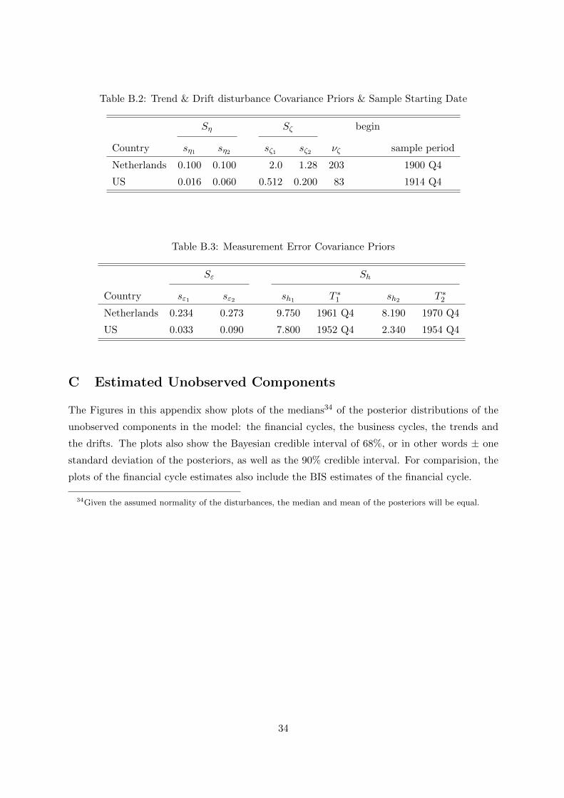
Section 5.4 Values for T ∗i are listed in Table B.2 in Appendix B.

The state equation of the state space form specifies the dynamics of the unobserved com-

ponents in the model. If we stack the unobserved components into a state vector ~at and the

unobserved component disturbances into the vector ~ξt, then the general expression of the state

equation is given by

~at+1 = Tt~at + ~ξt, (3)

where the matrix Tt is known as the transition matrix. This matrix is a sparse, block diagonal

matrix. This enables us to unpack the state equation into a number of separate equations, each

one governing the evolution of an unobserved component. We can therefore implicitly define

Tt by specifying these separate equations of each unobserved component. We begin with the

specification of the trend component ~µt.

The unobserved component ~µt in (1) represents a type of time-varying trend called a local

linear trend:

~µt = ~µt−1 + ~βt−1 + ~ηt, ~ηt ∼ N (0,Ωη) . (4)

Note that the covariance matrix Ωη is restricted to be diagonal to achieve a more parsimonious

model. The ~βt is an unobserved component that represents the time-varying growth rate of the

trend. It evolves as a random walk:

~βt = ~βt−1 + ~ζt, ~ζt ∼ N (0,Ωζ) (5)

The two components of the trend ~µt and ~βt together are responsible for the slowly changing,

growing trend in the data.

Both unobserved components ~ψFt and ~ψBt in (1) are cyclical components. In general a cyclical

component ~ψCt (where C = F indicates a financial cycle, and C = B a business cycle) evolves

4An alternative formulation could involve allowing for this type of time-varying change in the covariancematrices of the other unobserved components in the model. Experimenting with a model version in whichwe impose the time-varying structure in (2) on the trend disturbance covariance instead of the measurementdisturbance covariance makes no difference to the estimates we obtain for the rest of the model.

5

as follows. (~ψCt~ψC∗t

)= ρC

[cos 2π

λCsin 2π

λC

− sin 2πλC

cos 2πλC

]⊗ In

(~ψCt−1

~ψC∗t−1

)+

(~κCt

~κC∗t

)(6)

Note that we adopt the notation In to indicate the n× n identity matrix. Further we have that

~κCt ∼ N(0,ΩC

κ

)and ~κC∗t ∼ N

(0,ΩC

κ

). Also note that the covariance matrices of both distur-

bance vectors ~κCt and ~κC∗t are restricted to be equal, with ~κCt and ~κC∗t taken to be uncorrelated:

Cov(~κCt , ~κ

C∗t

)= 0. These restrictions are standard, see Harvey (1991) for details.

The dampening parameter 0 < ρC < 1 determines the persistence of the cycle ~ψCt , and

λC represents the period of the cycle.5 We note that the unobserved component ~ψC∗t is only

required for the construction of the cycle component ~ψCt . The specification is stationary and

ensures that when included in the measurement equation that the changes it induces in the data

are temporary.

The unobserved seasonal components ~γjt are also cyclical unobserved components with pe-

riods λj = 2π j4 and are constructed together with ~γ∗jt components in the same manner as in

(6). Note that j = 1, . . . , 2 in the case of quarterly data. Furthermore, for seasonal components

it is standard to impose the restriction that the dampening coefficient ρj = 1. The seasonal

component ~γjt is then given by the following.(~γjt

~γ∗jt

)=

[cosλj sinλj

− sinλj cosλj

]⊗ In

(~γj,t−1

~γ∗j,t−1

)+

(~ωjt

~ω∗jt

)(7)

Note that ~ωjt ∼ N (0,Ωω) and ~ω∗jt ∼ N (0,Ωω), where we impose the standard restriction that

the covariance matrices of ~ωjt and ~ω∗jt for j = 1, . . . , 2 are diagonal and equal. The reader is

referred to Harvey (1991) for further details.

2.1 Rank reduction

As currently specified, the model allows for a different financial cycle for each series. We are

however interested in the question of whether there is a single underlying financial cycle. In an

attempt to answer this question, we take the approach of imposing a single underlying financial

cycle in our model. We achieve this by restricting the rank of the covariance matrix of the

financial cycle components ΩFκ to 1 instead of the full-rank value of n. In this manner the

financial cycles for the series in the model are assumed to be driven by the same underlying

5The period of the cycle is given by 2π/λC . We assume a common dampening coefficients ρC and cycle periodλC . We also estimate model variants in which there is a dampening coefficient and cycle period for each series:ρCi and λCi . The restriction of common cycle parameters across series is supported by tests based on Bayes factorswhen we test whether the business and financial cycles each have their two own cycle parameters ρB , λB , ρF andλF that are shared across the series in the model.

6

stochastic process.

This rank reduction ensures that the financial cycles ~ψFt will be asymptotically the same up

to a scale factor determined by the size of the variances from the main diagonal of ΩFκ . This is

due to the fact that the presence of the dampening coefficient ρF in (6) ensures that the effect

of the starting values ~ψF1 and ~ψF∗1 becomes negligible as t→∞.

In order to ensure that we obtain estimates of the financial cycle ~ψFt (and of ~ψF∗1 ) that are

the same up to a scale factor from the beginning of the sample period t ≥ 1, we impose a prior

distribution of the starting values ~ψF1 and ~ψF∗1 in which the rank of their covariance matrices

are also reduced to 1. We obtain these priors from the steady state of the stationary process

defined in (6). This results in the following prior specification for the starting values:

~ψF1 ∼ N(

0,(

1− ρF 2)−1

ΩFκ

)and ~ψF∗1 ∼ N

(0,(

1− ρF 2)−1

ΩFκ

)(8)

We note that the prior specification for the starting values of the business cycle components,

~ψB1 (and of ~ψB∗1 ) is similar:

~ψB1 ∼ N(

0,(

1− ρB2)−1

ΩBκ

)and ~ψB∗1 ∼ N

(0,(

1− ρB2)−1

ΩBκ

). (9)

Although we do not impose rank reduction on ΩBκ , because here we are primarily concerned with

the estimation of the financial cycle, in future research we intend on exploring this possibility

as well.

In addition to the rank restriction on ΩFκ , we also impose restrictions on both covariance

matrices ΩBκ and ΩF

κ to require that their implied correlation between credit and the housing

price index be positive. In other words we assume that shocks to the financial cycle for credit and

the housing price index produce movement in the same direction for both cycles. Economically

this seems reasonable. In a financial boom, we would expect both credit and housing prices to

increase. It seems reasonably to assume that this should also hold for the business cycle. In

model versions which include the price to earnings ratio of the S&P 500, we also require that the

correlation with both credit and the housing price index be negative in the case of the financial

cycle, but positive for the business cycle. We note that these restrictions seem to have little to

no affect on our estimates.

An alternative, but equivalent approach to modeling a common trigonometric cycle compo-

nent is given in Koopman & Lucas (2005) and de Winter et al. (2017). The main difference with

our approach here is due to how the cycle components are formulated. In our model the mea-

surement equation (1) includes cycle components that are specified with correlated disturbance

terms. In the alternative model by comparison, there are n underlying cycle components which

by construction are independent. It is also possible to formulate an equivalent single financial

7

cycle in this alternative model. This would be based on the idea that the same underlying fi-

nancial cycle affects all n series in the model. This point is discussed in more detail in Appendix

A.

3 Estimation

Some of our data series consist of a combination of yearly and quarterly data. As a result,

our estimation procedure must be able to accommodate missing observations in the first three

quarters of each year in which we use annual data. We obtain our estimates of the financial

cycles using Bayesian MCMC simulation methods. Fortunately the estimation of state space

models with MCMC simulation methods in the presence of missing observations is possible and

is now standard, see for example Koopman et al. (1999).6 We wrote our own code to perform

the MCMC estimation in the matrix programming language OX, see Doornik & Ooms (2007).

MCMC simulation techniques are now standard, and we therefore do not discuss these sampling

methods in detail. We refer the reader instead to any textbook on Bayesian statistics, such as

Koop et al. (2007).

For most parameters it is possible to perform the simulation via the Gibbs sampler, or GS.

The simulation of the cycle component dampening parameters ρB and ρF and period parame-

ters λB and λF is not possible via the GS. In order to simulate these parameters we used the

Metropolis-Hastings algorithm, or MH algorithm. The imposition of rank reduction on the co-

variance matrix ΩFκ also introduces an additional degree of complexity to the MCMC simulation.

This involves both extra steps in the GS, as well as the use of the MH algorithm. We describe

these steps in We first briefly describe how the GS works with our model, and then discuss our

implementation of the MH algorithm. We then describe how we tackle the problems introduced

by the rank reduction in ΩFκ .

3.1 Gibbs Sampling

As is commonly done with state-space models, we augment the set of model parameters to

simulate in the GS with the disturbance terms from our model. Given values for the model

parameters, we can simulate the disturbances terms in our model using the disturbance smoother

as implemented in SsfPack, see Koopman et al. (1999) for details.7 Once we have simulated the

disturbance terms we then simulate new values of the covariance matrices of our model from

6We have encountered stability issues with the Kalman filter and related algorithms in certain areas of theparameter space of our model, introduced by the presence of missing observation at the beginning of the sampleperiod. However, in the relevant region of the parameter space for our estimation the Kalman filter-basedalgorithms remained well behaved.

7More computationally efficient sampling is possible, see Durbin & Koopman (2002).

8

their posterior distributions conditional on the drawn values of the disturbance terms. Given

the assumed normality of the disturbance terms in the model and the conjugate inverse Wishart

priors we specify on the covariance matrices of our model, the conditional posteriors from which

we draw the new covariance values also follow an inverse Wishart distribution: W−1 (ν, S). In

this standard case, we have that the posterior degrees of freedom ν is given by the sum of the

prior degrees of freedom νp and the number of observations, T : ν = T + νp. We also have that

the posterior parameter matrix S is equal to the sum of the prior matrix parameter Sp and the

sum of outer product of the residual vector R: S = Sp +R.

In general the GS works by repeatedly cycling through the two simulation blocks of drawing

the disturbances and drawing the covariances. Asymptotically, by repeatedly re-simulating all

the values, we obtain drawings from the unconditional joint posterior of the model parameters

and disturbances.8 This is however only true if we can also include a method to obtain updated

drawings for ρB, ρF , λB and λF , as well as for the reduced rank covariance matrix ΩFκ . Drawing

ρB, ρF , λB and λF is not feasible in the GS as we do not know any easily derived conditional

posterior from which we could draw new values. Instead we use the MH algorithm.

θ\i

3.2 Metropolis-Hastings Algorithm

We use the MH Algorithm when we are unable to draw new parameter values directly from the

appropriate conditional posterior required by the GS. Instead we draw a new parameter value

from a candidate distribution. We either accept this new draw, or reject it and keep the original

value from the previous draw. The decision to reject or accept the candidate drawing is based

on the value of δc:

δc =P (θ∗i )L

(Y |θ∗i , θ

(m−1)\i

)fc

(θ

(m−1)i |θ∗i

)P(θ

(m−1)i

)L(Y |θ(m−1)

i , θ(m−1)\i

)fc

(θ∗i |θ

(m−1)i

) . (10)

When δc ≥ 1 we automatically accept the candidate value. When δc < 1 we accept the candidate

value with probability δc. Note that in (10) P (θ∗i ) represents the prior density of the parameter

θi at the value given by the candidate drawing θ∗i at step m of the MCMC algorthim. The

value of the previous draw is denoted by θ(m−1)i . The value of the likelihood given the candidate

parameter value θ∗i and the other model parameters values in the MCMC algorithm θ(m−1)\i is

denote by L(Y |θ∗i , θ

(m−1)\i

). The density of the parameter value θ∗i obtained from the candidate

8Via the disturbances we can also obtain drawings of the state vector: the trend, growth rate, cycles andseasonal components. The reader is referred to Koopman et al. (1999) for details.

9

density function is then given by fc

(θ∗i |θ

(m−1)i

). Note that the form of the candidate density

can depend on the previously drawn parameter value θ(m−1)i . In our implementation this is the

case.

For the cycle period parameters λB and λF we draw candidate values from the gamma

distribution with an expected value equal to the previously drawn period value. Similarly for

the dampening coefficients ρB and ρF we draw candidate values from the beta distribution also

with an expected value equal to the previously drawn dampening coefficient value.9 We obtain

the required values of the likelihood from the diffuse Kalman Filter based on the prediction error

decomposition of the likelihood. In our program we perform one Metropolis-Hastings rejection

step for the four cycle parameters jointly.10

3.3 Sampling ΩFκ with Rank Reduction

In the presence of rank reduction, such as we impose on ΩFκ , drawing a new value for the

covariance matrix is more complicated. Part of the covariance matrix can be simulated via

the GS. The rest we draw using the MH algorithm. To see how we use the GS here, let us

consider the general case of the covariance matrix ΩC which has the reduced rank of r < n. We

begin by first drawing a new value for ΩC given the current simulated values of the associated

disturbances ~κCt , t = 1, . . . , T . Given the newly simulated value of ΩC we then draw new values

of the disturbances ~κCt , t = 1, . . . , T to complete the required GS steps.

We begin with the GS draw of ΩC , and denote the conditional posterior of ΩC in the GS

by W−1(νC , SC

). Now consider the eigenvalue decomposition of the n × n parameter matrix,

SC = EΛE′, where the matrix of orthonormal eigenvectors E is given by E = [~e1, . . . , ~en] such

that E′E = the n× n identity matrix In, and Λ is a diagonal matrix with the eigenvalues λSi,

i = 1, . . . , n along its diagonal. SC has the reduced rank of r < n. If we order the eigenvalues

from largest to smallest, then we have that λS,n−r+1 = . . . λSn = 0. We can then denote the

n × r matrix of r eigenvectors corresponding to the r non-zero eigenvalues as Er = [~e1, . . . , ~er],

and in the same manner the r × r diagonal matrix of non-zero eigenvalues as Λr. We can now

re-write SC as follows.

SC = ErΛrEr′ (11)

To obtain a draw for the reduced rank covariance matrix ΩC from the inverse Wishart distribu-

9This leaves an additional distribution parameter to be fixed, both in the case of the gamma and of the betacandidate distributions. We tune this value to ensure a rejection rate of between 20% and 50%.

10We repeat these joint MH drawings eight times in each cycle through the GS. The number 8 was arbitrarilychosen to produce more draws than for the parameters drawn from Gibbs sampling, because we assume that thesedraws require more replications to achieve convergence.

10

tion W−1(νC , SC

), we define the matrix ΣC :

ΣC = ErΛ12r . (12)

Then we draw the r × r full rank matrix X from the standard Wishart distribution: X ∼W(νC , Ir

)and obtain

Q = ΣCXΣC ′. (13)

We now perform the eigenvalue decomposition of Q, which is n × n and of rank r, so that

Q = EQrΛQrE′Qr as in (11). The reduced rank drawing ΩC for the covariance ΩC is then given

by

ΩC = EQrΛ−1QrE

′Qr. (14)

To complete the required steps of the GS for our model, we must now draw new values of

for the disturbances ~κFt , t = 1, . . . , T . However, this is also more complicated than for the other

disturbances associated with the unrestricted covariances in the model. The reduced rank of ΩFκ

causes statistical degeneracy in the joint distribution of the disturbances ~κFt , t = 1, . . . , T . For

this reason in our model we can only draw r of the n vectors ~κFt , t = 1, . . . , T in the disturbance

smoother, see Koopman et al. (1999) for a detailed discussion.

To draw the n × 1 disturbance vectors κCt , t = 1, . . . , T given the newly drawn covariance

matrix ΩC with rank r < n, we assume that we have ordered the disturbance vectors ~κCt and

ΩC so that we have

~κCt =

(~κCat

~κCbt

), (15)

where ~κCat represents the r elements of ~κCt that we can simulate with the disturbance smoother,

and ~κCbt represents the n− r remaining disturbances that we cannot obtain from the disturbance

smoother due to the problem of statistic degeneracy caused by the rank reduction.11 Similarly

to (12), from the eigenvalue decomposition of ΩC in (14), we then define

Σ = EQrΛ− 1

2Qr . (16)

As a result, ΩC = ΣΣ′. Therefore, we have that the newly simulated values κCat of the distur-

11The disturbance smoother in SsfPack requires the specification of the diagonal selection matrix Γ which is thesame dimension as the state vector with either ones on the diagonal or zeros for the corresponding stochasticallydegenerate elements of the state. Therefore, in our estimation procedure, Γ specifies the r elements of ~κCat, seeKoopman et al. (1999) for details. We adjust the value of Γ so as to select the r series with the strongest cycleestimates, because we believe this may aid convergence.

11

bances ~κCat, t = 1, . . . , T must satisfy the following.

κCt =

(κCat

κCbt

)= Σεt =

[Σa

Σb

]εt, (17)

where ~εt ∼ N (0, Ir) is an unknown r × 1 vector of disturbances. Furthermore Σa is r × r and

Σb is (n− r)× r, both sub-matrices of Σ, such that

ΩC =

[ΣaΣa

′ ΣaΣb′

ΣbΣa′ ΣbΣb

′

]. (18)

Given the simulated values κCat from the disturbance smoother, we can solve (17) to obtain the

following.

εt = Σ−1a κCat, (19)

Note that Σ−1a exists because the r× r sub-matrix ΣaΣa

′ from the top left corner of ΩC in (18)

has full rank by construction.12 By combining the results from (17) and (19), we can see that

we can recover κCbt from the following.

κCbt = ΣbΣ−1a κCat (20)

We have now obtained the simulated disturbances κCt , t = 1, . . . , T , which, together with the

simulated covariance matrix ΩC completes the required steps of the GS. This leaves only the

steps of the MH algorithm to ensure that ΩFκ is correctly simulated.

To see why we still require additional sampling, consider the rank reduction on ΩFκ where

r = 1, In (13) the draw X is a scalar, whereas the complete draw ΩFκ requires n parameters:

one for each of the n variances, with the covariance being determined by the perfect correlation

implied by the rank reduction. Clearly these GS steps only manage to simulate one of the

required parameters in ΩFκ . An additional set of steps using the MH algorithm is required to

ensure that we fully sample a new value for ΩF .

In the general case outlined above, the simulated value X in (13) is an r × r symmetric

matrix, and therefore is implicitly only defined by r (r + 1) /2 univariate elements. In general

the n× n covariance matrix ΩFκ of rank r < n is defined by

n (n+ 1)− (n− r) (n− r + 1)

2>r (r + 1)

2(21)

univariate elements.

12This is due to the assumed ordering of the disturbance vector κCt in (15).

12

Similarly, if we examine (17), we can see that the disturbance smoother only implicitly

simulates the r × 1 vector εt. Because κCat = Σaκεt, there is new information in the conditional

posterior distribution of ΩFκ to define a new drawing of Σaκ. We can also see, however, from (19)

and (20), that the information in the r × 1 drawing εt is recycled to obtain the (n− r) vector

κbt. There are therefore no new stochastic univariate elements used to construct the (n− r)× rmatrix Σbκ, which defines part of the conditional posterior of ΩC

κ in the Gibbs sampling draw

discussed above.

We have observed in practice that the term ΣbΣ−1a in (20) remains constant in our applica-

tions when r = 1. In general we denote this (n− r)× r matrix as B:

B = ΣbΣ−1a . (22)

We vectorize the elements of B and draw them as B∗ from a multivariate normal candidate

distribution, N(B(m−1), SB

), where SB is a diagonal matrix of variances for the vectorized

elements of B, and B(m−1) is the previous draw of the elements of B. The variances in SB must

be set to be able to perform this application of the Metropolis-Hastings step.13

We note that to obtain a complete simulation of the financial cycle vector ~ψCt for t = 1, . . . , T

we require the simulated starting values ψC0 , which we can straight-forwardly obtain from the

simulation smoother. Draws for the other set of cycle disturbance vectors ~κC∗t , as well as the

cycle components ~ψC∗t for t = 1, . . . , T can be obtained in the same manner as outlined above.

Once the MCMC algorithm has converged we continue to run the simulation steps to obtain a

sample from the joint posterior distribution. We can then base our inference on this sample.

Standard diagnostics can be used to check for the convergence of the MCMC algorithm.

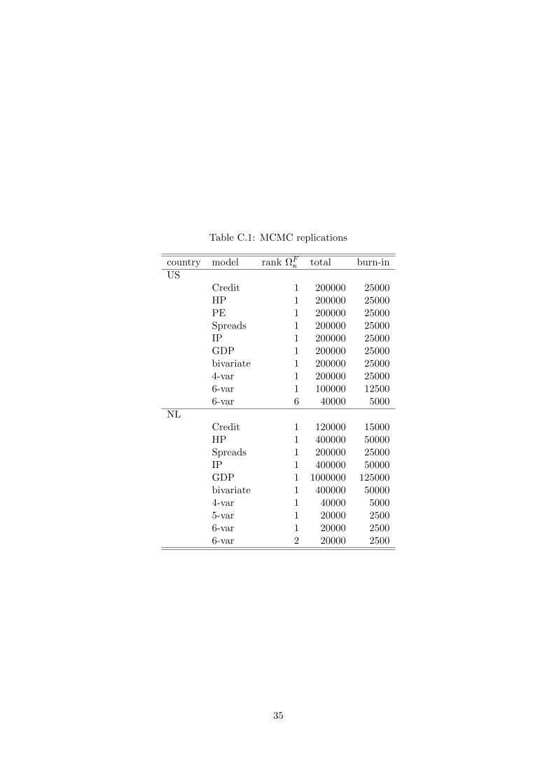
Most of our results are based on a total of 200,000 replications from 4 parallel chains for each

country model, where we throw away the first half of the replications from each chain as burn-in

to ensure that we only sample from the MCMC algorithm once convergence has been achieved.

Convergence diagnostics indicate that our MCMC algorithm has converged, the details of which

are available on request. The exact number of replications for each model is listed in Appendix

C in Table C.1.

4 Priors

The model we propose has a fair number of parameters, making the model quite flexible. There

are therefore parameter regions that we would prefer to rule out. We achieve this using somewhat

informative prior on some of the parameters. We also specify weakly informative priors to help

13Through experimentation we tune these variances to produce a rejection rate of between 20% to 50% for thejoint test of the elements of B.

13

achieve our business and financial cycle decompositions with cycle periods for the business cycle

that are relatively short and for the financial cycle that are relatively long. For the other priors

we specify a small number of degrees of freedom and select the prior scaling factor centered

around the main posterior density mass. In this way we specify fairly uninformative empirical

Bayes priors. We discuss the various prior specifications we use for each unobserved component.

4.1 Cycles

Both cycle components require priors for the dampening coefficients ρC , the cycle periods λC ,

and the disturbance covariance matrices ΩCκ , for C = B and F , see (6) above. Given that the

dampening coefficients 0 < ρC < 1, we specify a beta distribution for these priors. Note that

apriori we want ρC < 1 to ensure that the cycle components are stationary and that the cycle

disturbances have no permanent effects on the long run level of the series. The priors for the

cycle periods λC ∈ (4,∞) for quarterly data, follow gamma distributions. The priors for the

covariance matrices ΩCκ are inverse Wishart distributions.

The beta priors are parameterized as Beta(αCp , β

Cp

), for C = B and F .14 For the business

cycle component, ρB, we set αBp = 55.88 and βBp = 1.925. This implies a prior mean of 0.967,

with a standard deviation of 0.0234. This prior relatively diffuse and has little impact on the

posteriors. The prior parameters for the financial cycle components’ parameter ρF , are give by

αFp = 321.3 and βBp = 4.617. These parameters imply a posterior mean of 0.986 and standard

deviation of 0.0065. Although this prior is more spread out than the posteriors, the posteriors

tend to lie slightly above the prior. This prior is therefore somewhat informative in that it tends

to pull the posterior away from the value of 1. Experimenting with differing prior parameters

suggests that our results are not very sensitive to this prior.

The prior gamma distribution for the λC is denoted by Gamma(aC , bC

), for C = B and

F .15 These priors are formulated using a Bayesian highest density region, or HDR. In the case

of the business cycle, we make the prior assumption that the probability that the business cycle

period is between five to ten years is 99%: P(20 quarters < λB ≤ 40 quarters

)= 99%. This

results in the prior parameter values of aB = 55.88 and bB = 4.617 for the gamma prior of λB.

We formulate our prior for the financial cycle period λF in a similar fashion. Here we employ the

99% prior HDR of between 15 to 20 years: P(60 quarters < λF ≤ 80 quarters

)= 99%. This

implies the prior parameter values of aF = 321.3 and bF = 1.925 for the gamma prior of λF .

Alternative priors based on the same HDR intervals, but with lower probabilities, such as 95%

or 90%, result in similar estimates. If, however, we increase these intervals to encompass longer

periods, then this can alter our estimates. For example an HDR for λF based on the interval

14The density function of Beta (αp, βp) is then given by f (x) = xαp−1 (1− x)βp−1 /B (αp, βp).15The density function of Gamma (a, b) is then given by f (x) = ba

Γ(a)xa−1 exp−b x.

14

from 20 to 25 years tends to result in somewhat different financial cycle estimates. On the

whole, however, we believe that our priors for the cycle periods represent the values most cited

in the literature, see for example Drehmann et al. (2012) and Borio (2014). Although somewhat

informative, these priors still allow the posteriors to be largely determined by the data.

We denote the prior inverse Wishart distribution for ΩCκ by W−1

(νC , SC

), for C = B and

F .16 The prior parameter νC represents the number of degrees of freedom. For both the business

and financial cycle we set νB = νF = 10 + n. We then select the positive (semi) definite matrix

S to ensure that the mean of the posterior is unaffected by the prior. These values for SC for

C = B and F are listed in Table B.1 in Appendix B for our preferred bivariate model variant.

The prior parameters used in other model variants are available on request.

4.2 Trend & Growth Rates

The two trend components µi,t in (4) and the two growth rates βi,t in (5) follow random walks.

They are therefore non-stationary. As a result we assume diffuse priors for their initial values.

The inverse Wishart prior degrees of freedom for the disturbance covariance matrices Ωη for

the trend component and Ωζ for the growth rate component are νη = 10 + n and νζ = 200 + n,

respectively. The values for the prior parameter matrices Sη and Sζ are listed in Table B.2 of

Appendix B.

In general 10+n degrees of freedom for the inverse Wishart distribution produces a prior that

is relatively uninformative. We select the values for Sη to ensure that the highest prior density

region corresponds to that of the posterior.17 In this way the priors for Ωη are selected to have

minimal impact on the form of the posteriors. This essentially an empirical Bayes approach.

Our prior specification for the Ωζ are more informative. We interpret the drift components

~βt as representing the underlying growth rates. As such we believe apriori that these rates

will only change gradually over time. It is however common in SSM’s of macroeconomic time

series with a local linear trend, such as we have specified here, that the likelihood tends to favor

larger values for the variance of the disturbance of the drift component. These larger values

for the variance imply a relatively quickly changing growth rate. In the case of our model we

believe that these changes ought to be captured by the cycles in the model. For this reason

we specify the larger prior parameter value of νζ = 200 + n in model variants with a longer

sample period, and 80 +n otherwise for Ωζ of the growth rate component. This then represents

16The density function of W−1(νC , SC

)is then given by

f (X) =|S|ν/2

2νΓ2

(ν2

) |X|−(ν+3)/2e−12tr(SX−1)

.17The off-diagonal elements of Sη are zero, because Ωη is diagonal. These priors are therefore equivalent to

inverse-gamma priors with the inverse gamma distribution parameters αηi = νη/2 and βηi = sηi/2, i = 1, . . . , n.

15

a more informative prior. Compared with the information in a sample period of more than

200 observations, this number of degrees of freedom is still fairly modest. We specify diagonal

elements of the prior parameter matrices Sζ which correspond to modest changes over time in

the growth rates βi,t. The off-diagonal elements are assumed to be zero indicating a prior of no

correlation between the n growth rates.

In those instances where the marginal posterior variance for ζit was lower than our initial

prior specification would suggest18, we lowered the corresponding value in Sζ to match the

posterior.

4.3 Seasonal Components

The covariance matrices Ωω1 and Ωω2 in (7) are assumed to be diagonal. Therefore the prior

parameter matrices Sω1 and Sω2 are as well. In all cases we set the number of degrees of freedom

of these inverse Wishart priors to νω1 = νω2 = 10 + n and

Sω1 = Sω2 =

c 0

. . .

0 c

, (23)

where usually c = 0.0002. With the exception of the US industrial production series, all series

exhibit only a slight degree of seasonality.19 We specify diffuse priors on the initial values γi,j,0

and γ∗i,j,0, because these components are non-stationary.

4.4 Measurement Error Covariance

To specify a prior on the covariance matrix Ωε,t of the measurement error as given in (2), we

need to specify priors on the diagonal matrices Ωε and Ωh where their main diagonals are given

by the following vectors.

diagonal (Ωε) = (σε1 , . . . , σεn) , diagonal (Ωh) = (σh1 , . . . , σhn) . (24)

We use inverse Wishart priors: P (Ωε) ∼ W−1 (νε, Sε) and P (Ωh) ∼ W−1 (νh, Sh). We can define

the diagonal matrices Sε and Sh as follows.

diagonal (Sε) = (sε1 , . . . , sεn) diagonal (Sh) = (sh1 , . . . , shn) (25)

In Table B.3 of Appendix B we list the elements of the prior parameter matrices Sε and

18We initially specify a prior on Ωζ that implies an expected value of 0.08 for each σζi , i = 1, . . . , n.19For this reason we set C = 0.015 for US IP.

16

Sh for our preferred bivariate model.20 We also list in this table the dates T ∗i when our model

transitions to the lower measurement error variance, see (2). We set the degrees of freedom

νε = νh = 40. We adjust the non-zero values in Sε and Sh until the posterior is centered around

the prior. The exception to this is Dutch industrial production, where we held the prior mode

below the posterior to ensure the stability of the Kalman Filter in the estimation procedure.

The prior values we specify for the other model variants are available on request.

5 The data

We include up to six data series in our multivariate models of the US and of the Netherlands:

credit, a house price index, GDP, industrial production, and two other indices which we con-

struct, one based on the the S&P500 PE ratio, and the other based on interest rate spreads. Plots

of these data series are given in Appendix C together with their estimated trend components

from various SSM variants in the case of the credit, housing price index, industrial production

and GDP. The plots of the first difference of the cumulated S&P 500 PE and spreads data are

shown together with their estimated drift components from various SSM variants. In the case

of these latter two series, the first difference corresponds to the original data before cumulation,

and these plots show the data more clearly than the trend does.

We discuss here the sources and definitions of the data and describe how we transform the

data for the model. All series are analyzed on a quarterly basis21, with missing values for the

missing quarters for the periods when we only have annual data available. When the orginal

data series are monthly, we use the index value from the end of the month of the last month in

each quarter as the quarterly value.

5.1 Credit & House Prices

The credit series is for total credit to the private non-financial sector, measured as the stock

of outstanding credit at the end of the quarter. This credit series and the housing price index

are both published by the Bank of International Settlements, or BIS on a quarterly basis. For

earlier values, when no quarterly values are available, we rely on the yearly credit data published

in Jorda et al. (2017) and the yearly housing price indices published in Knoll et al. (2017). In

20Given that the measurement errors between the n series are uncorrelated, these priors are equivalent toinverse-gamma priors on σεi and σhi with the inverse-gamma distribution parameters αεi = νε/2, αhi = νh/2,βεi = sεi/2 and βhi = shi/2, where i = 1, . . . , n.

21We have also produced estimates based on monthly observations of industrial production, spreads, and theS&P500. the results we obtain are similar. The estimation based on monthly data however involves the introduc-tion of a substantial number of missing values, because credit, housing prices and GDP are quarterly series. Thisslows down the estimation and in some cases causes numerical instability in the Kalman Filter which we use inour estimation procedure.

17

this case the annual data represents a fourth quarter measurement, and the first three quarters

of the year are missing.

Both the credit series and housing price indices are deflated using consumer price indices. In

the case of the US data, we obtained monthly CPI data from Schiller (2015). The Dutch CPI

data came from the US Federal Reserve’s Federal Reserve’s FRED Economic Data,22 but the

source of the data is the OECD’s “Main Economic Indicators - complete database”.

Inspection of the data indicates that the earlier yearly data is more volatile. This motivated

our decision to use the split measurement error variance in (2). We identify the transition dates

T ∗i in (2) when the data transitions to a lower level of variability for the credit and housing

price indices by determining when the data comes from a more reliable source. We were able to

determine this based on the information in the documentation of the data series given in Jorda

et al. (2017) for the credit data and in Knoll et al. (2017) for the housing price indices. These

dates are listed in Table B.3 of Appendix B.

5.2 S&P 500

We construct a earnings to price ratio index from the S&P 500 stock price index, earnings, and

the US CPI data. The data are available from Schiller (2015). Stock prices are the real total

return price. Earnings are given by the real total return of the scaled earnings.23

The Dutch stock index the AEX is only available starting in 1983, which does not represent

a sufficiently long sample for this study. We therefore rely on the correlation between the US

and Dutch economy to justify the use of the S&P 500 data in the Dutch model as well.

We transform the earnings Et and price Pt data to obtain a growing index that we can

model using the local linear trend specification in (4.) We start with the earnings to price ratio,

βept = EtPt

which we can think of as a rate of return. We therefore aggregate these growth rates

into an index, starting at the arbitrary value of 100. We then transform this index using the

logarithm to obtain the series lept, which is then given by24

lept = 100 log

100t∏

j=1

(eβ

epj

) 112

= lep0 +100

12

t∑j=1

βepj (26)

To see that this definition of the index lept results in a series much like the credit or housing

price index, first consider a level series Yt, such as credit or the house price index, with growth

22Available from their website https://fred.stlouisfed.org

23The data appears to be dated as if it is measured at the first of each month. However, comparison with theon-line data for the S&P 500 suggests that the data is from the end of the month. We date the data in our modelas being measured at the end of the month.

24We take the twelfth root to reduce the dramatic growth of the index over the sample period. This simplyrepresents multiplication of the logged index by a constant.

18

https://fred.stlouisfed.org

rate βyt . We have then that

Yt = Y0

t∏j=1

(1 + βyj ) ≈ Y0

t∏j=1

eβyj = Y0 exp

t∑j=1

βyj

. (27)

Transforming the data series using logarithms then leads to the following expression.

yt ≡ 100 log (Yt) = y0 + 100t∑

j=1

βyj (28)

We can see that this expression has essentially the same structure as lept in (26).

5.3 Interest Rate Spreads

We opt to include the spreads, st in our model also by transforming the series into an index in

much the same manner as we do with the S&P 500 data. It seems reasonable to consider the

relevant data as being the difference between the price level of the risky and safe bonds, or of

short and long run bonds. As we show below, this turns out to be the same as the aggregated

spread series. As we argue above for the S&P 500 data, this fits best with how we model for the

level UC in (4).

To see how we construct an index based on the interest rate spreads, consider the bond price

of a safe bond, Blt and the price of a risky bond Bk

t . The relevant series which best matches

the other level series in the model is given by the ratio between the prices of the risky and safe

bonds from the spread:

Bkt

Blt

=Bk

0

Bl0

t∏j=1

(erkj

erlj

) 112

= Bkl0

t∏j=1

(erkj−rlj

) 112

= Bks0

t∏j=1

e112st . (29)

Here the interest rate spread st is the difference between the annual risky interest rate, rkt and

the annual safe interest rate, rlt: st = rkt − rlt. Note that (29) is similar to (26) for the level

transformation lept based on the S&P 500 data, and to (28) for Yt.

We can now take the logarithm of this bond price ratio series. This results in the cumulative

sum of the interest rate spread:

blst ≡ 100 log(Blst

)= bls0 +

100

12

t∑j=1

sj . (30)

For the US, we construct an index based on Moody’s seasoned AAA corporate bond minus

the federal funds rate. This series is available on a monthly basis and is not seasonally adjusted.

19

The sample period begins in July of 1954, and is available until January 2019. This series

represents the best compromise between a good measure of the interest rate risk spread and a

series of sufficient length to study the financial cycle.

No spreads of sufficient length are available for the Netherlands. Instead we use the difference

between the ten year interest rates on government bonds and the three month interbank rate for

Germany. This data is available from the US Federal Reserve’s Fred Economic Data.25 This data

goes back to January 1960 on a monthly basis. We assume that the strong correlation between

the German and Dutch economy is sufficient to justify using this German series together in a

Dutch model.

5.4 Industrial Production & GDP

A seasonally-unadjusted monthly index series of US industrial production (IP) is available start-

ing in January of 1919 from the US Federal Reserve’s FRED Economic data. We also obtained

Dutch IP data from the FRED. The Dutch data is seasonally adjusted, monthly data. This

series starts in January of 1960.

Data for the gross domestic product (GDP) of the US and the Netherlands is only available

on a quarterly basis. The US no longer publishes seasonally-unadjusted data for US GDP. We

therefore use real US seasonally-adjusted quarterly GDP starting in the first quarter of 1947.

This data is published by the US department of Commerce’s Bureau of Economic Analysis.26

The Dutch CBS does not publish real quarterly GDP for the Netherlands before 1995.However,

real seasonally-adjusted quarterly GDP figures for the Netherlands are available starting in the

first quarter of 1960 from the US Federal Reserve’s FRED Economic Data.

6 The results

In this section we present the financial cycle estimates. In particular we want to gauge how

successful the rank reduction on ΩFκ is as a method of identifying a unique financial cycle. We

also want to determine which series are most informative about the financial cycle, and which

model variants are best suited to the estimation of the financial cycle.

We estimate a number of multivariate model variants for the US and the Netherlands, as

well as a univariate variant for each series. We begin with a bivariate model based on credit

and the housing price index. The motivation for a model based on credit and the housing price

index is that, as our results below show, the financial cycle in the US and the Netherlands is

primarily determined by these two series. An additional advantage of modeling these two series

25Available from their website https://fred.stlouisfed.org.26The data is available from their website https://www.bea.gov/iTable/index_nipa.cfm.

20

https://fred.stlouisfed.org

https://www.bea.gov/iTable/index_nipa.cfm

together is that the resulting sample period is long. In the case of the US, the sample period

runs from fourth quarter of 1914 (following the creation of the US Federal Reserve system) until

the second quarter of 2018. For the Dutch data the sample period begins in the fourth quarter

of 1900 and runs until the second quarter of 2018.

We also estimate six-variable model variants for the US and the Netherlands based on all

the available series. In the case of the US, the sample period runs from the fourth quarter of

1954 until the fourth quarter of 2018.27 The six-variable Dutch variant has a sample period that

spans the period of the first quarter of 1960 until the first quarter of 2019.28 For the Dutch data

only credit and the housing price index are available before 1960. The six-variable Dutch model

includes the US S&P 500 series lept, even though this series is for the US. The spreads series

we use in this case is also for Germany, not the Netherlands, but we suppose a high degree of

integration between the US, German and Dutch financial markets and for this reason estimate

this six-variable Dutch model with the rank of ΩFκ restricted to be 1 and 2. Alternatively, we

also estimate a Dutch five-variable model variant which excludes the S&P 500 data.

Finally we also estimate four-variable model variants. In the case of the US data, this model

includes credit, the housing price index, the S&P 500 series and IP. This combination of series

still allows us to use a long sample period that runs from the fourth quarter of 1919 until the

final quarter of 2018. The Dutch four-variable variant also includes credit, the housing price

index and IP, but swaps the the S&P 500 series our for the Germany spreads. The sample period

for this model runs from the first quarter of 1960 until the first quarter of 2019.

6.1 The Financial Cycle with rank ΩFκ = 1

In this section we compare the estimates of the financial cycles we obtain from the model variants

in which we restrict the rank of ΩFκ to be 1 to ensure a single underlying financial cycle. The

figures are based on the posterior median of the financial cycle and the 68% and 90% credible

regions. They also include estimates of the financial cycle produced by the BIS which start in

1970 (see Drehmann et al. (2012)).

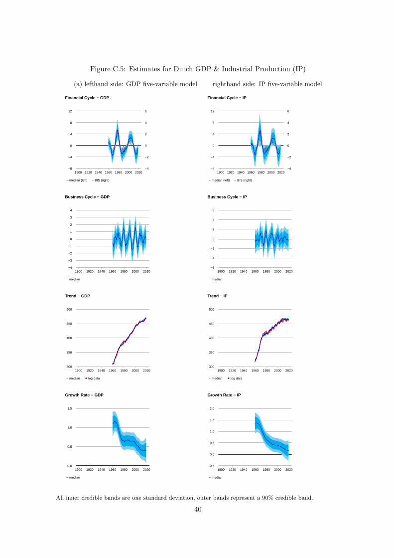
We note that Appendix C includes additional figures showing plots of the financial cycles

based on the other series for selected model variants. These figures also include plots of the

business cycles, trends and drifts. The plots of the estimated trends also include the observed

series, or in the case of the S&P 500 PE and Spreads cumulated series, the plots of the estimated

drifts include the first difference of the series.29

Here in Figure 1 we show the estimates we obtain based on the US credit and housing price

27The US spreads are not available before 1954.28Note that some series in these models having missing observations at the end of the sample period.29Plots for the other model variants as well as of the estimated seasonal components are available on request.

21

index for all four model variants. The match with cycle based on the univariate model of the

housing price index with the multivariate estimates is close. The univariate model of credit

on the other hand produces a somewhat different cycle. This suggests that the multivariate

cycle estimates are more strongly determined by the housing price index than credit. The three

multivariate variants produce very similar financial cycle estimates. The bivariate variant has

the additional benefit of being based on a longer sample period and so producing a financial

cycle estimate covering a longer period.

In Figure 2 we can compare the estimated financial cycles based on credit and the housing

price index for the Netherlands. This figure excludes the estimates from the six-variable model

variant, which we discuss below. As is the case with the US results, these three multivariate

variants also produce similar financial cycle estimates, with the bivariate variant benefiting from

a longer sample period. The estimates based on the credit series, however, now seem somewhat

weaker. This is an indication that the Dutch financial cycle is dominated by the housing price

index.

We can gauge the plausibility of our financial cycle estimates based on known historical events

such as the Great Depression as well as the recovery led by World War II and its aftermath, the

US savings and loans crisis of 1986, and the Great Recession30 In the case of the Netherlands

we can also see the effects of the housing boom from 1976-78 and the crash that followed from

1979-1983. We can see these events reflected in the estimates by a drop in the financial cycle

during weaker periods and an increase during stronger periods. We also note that our estimates

also show a substantial level of agreement with those of the BIS.

More generally, the mean posterior values for the period of the financial cycles, λF of the

model variants were between 67 to 76 quarters, or roughly 17 to 19 years. Values for the posterior

means from the bivariate model variants are given in Table E.3 in Appendix E. For the business

cycle we obtained posterior mean values for λB of between 8 to 11 years. These values are also

listed in Table E.3 for the bivariate models. They are in close agreement with standard values

for the business cycle in the literature. Appendix E also lists the posterior means and standard

deviations for the other parameters for the bivariate models, see Tables E.1, E.2 and E.3.

The concordance index between cycles provides us with an additional measure of the extent of

agreement between the various financial cycle estimates. A value approaching 1 indicates a nearly

perfect agreement between the cycles, whereas a value approaching 0 indicates a nearly perfect

counter-cyclical relationship. An expected value assuming no relationship can be calculated for

comparison. This value will typically be near 0.5. In Table 1 we list the concordance index

between the estimated US financial cycles for each model variant, including the financial cycle

estimate of the BIS. Table 2 provides the same information for the Dutch estimates. Tables of

30See Reinhart & Rogoff (2009) and Laeven & Valencia (2012) for further details on systemic banking crises.

22

Figure 1: Financial cycle estimates for US credit & housing price index

1900 1920 1940 1960 1980 2000 2020−16

−12

−8

−4

0

4

8

12

16

−4

−3

−2

−1

0

1

2

3

4

Financial Cycle − Credit

median (left) BIS (right)

(a) Univariate

1900 1920 1940 1960 1980 2000 2020−40

−30

−20

−10

0

10

20

30

40

−4

−3

−2

−1

0

1

2

3

4

Financial Cycle − HP


(b) Univariate

1900 1920 1940 1960 1980 2000 2020−16

−12

−8

−4

0

4

8

12

16

−4

−3

−2

−1

0

1

2

3

4



(c) Bivariate

1900 1920 1940 1960 1980 2000 2020−40

−30

−20

−10

0

10

20

30

40

−4

−3

−2

−1

0

1

2

3

4



(d) Bivariate

1900 1920 1940 1960 1980 2000 2020−16

−12

−8

−4

0

4

8

12

16

−4

−3

−2

−1

0

1

2

3

4



(e) four-variable

1900 1920 1940 1960 1980 2000 2020−40

−30

−20

−10

0

10

20

30

40

−4

−3

−2

−1

0

1

2

3

4



(f) four-variable

1900 1920 1940 1960 1980 2000 2020−16

−12

−8

−4

0

4

8

12

16

−4

−3

−2

−1

0

1

2

3

4



(g) six-variable

1900 1920 1940 1960 1980 2000 2020−40

−30

−20

−10

0

10

20

30

40

−4

−3

−2

−1

0

1

2

3

4



(h) six-variable

All inner credible bands are one standard deviation, outer bands represent a 90% credible band.

23

Figure 2: Financial cycle estimates for NL credit & housing price index

1900 1920 1940 1960 1980 2000 2020−4

−2

0

2

4

6

−4

−2

0

2

4

6



(a) Univariate

1900 1920 1940 1960 1980 2000 2020−40

−20

0

20

40

60

−4

−2

0

2

4

6



(b) Univariate

1900 1920 1940 1960 1980 2000 2020−10

−5

0

5

10

15

−4

−2

0

2

4

6



(c) Bivariate

1900 1920 1940 1960 1980 2000 2020−40

−20

0

20

40

60

−4

−2

0

2

4

6


median (left)

(d) Bivariate

1900 1920 1940 1960 1980 2000 2020−10

−5

0

5

10

15

−4

−2

0

2

4

6



(e) four-variable

1900 1920 1940 1960 1980 2000 2020−40

−20

0

20

40

60

−4

−2

0

2

4

6



(f) four-variable

1900 1920 1940 1960 1980 2000 2020−10

−5

0

5

10

15

−4

−2

0

2

4

6



(g) five-variable

1900 1920 1940 1960 1980 2000 2020−40

−20

0

20

40

60

−4

−2

0

2

4

6



(h) five-variable


24

the expected values assuming no relationship can be found in Appendix D.

In the case of Table 1 for the US, we can see that the estimates from the univariate models

of credit and the housing price index show a high degree of concordance with the multivariate

estimates and with the BIS. This is also the case for the bivariate model based on credit and

the housing price index. This leads us to conclude that these two series are the most important

determinants of the financial cycle. Relative to the expected values listed in Table D.1, the other

series seem to have a weaker relationship with the US financial cycle.

In general the concordance values between the univariate estimates based on the S&P 500

and spreads and the other model variants suggests that these two series have a counter-cyclical

relationship with the financial cycle, albeit a weak one.31 This can also be seen in the plots

of the financial cycle based on PE and the spreads shown in Figure C.2a. The values of the

concordance between the IP estimates and the other model variants shows no consistent pattern,

indicating that IP is not strongly influenced by the financial cycle. GDP seems to have a positive

relationship with the financial cycle, perhaps due to the contribution of financial sector. However

this relationship also seems to be weak.

Table 2 for the Netherlands indicates broadly the same patterns. Credit, however, seems

to produce a counter-cyclical financial cycle from its univariate model, although inspection of

the plot of the estimated cycle in 2a suggests that this cycle is weak. This suggests that the

Dutch financial cycle is largely driven by the housing price index. We note that the concordance

between the financial cycle from the bivariate model and the cycles from the other multivariate

models and the BIS is even larger than is the case for the US results.

Table 1: Concordance between US financial cycle estimates

Model Univariate Bivariate 4-vars 6-vars BIS

Variable HP PE IP GDP Spreads

UnivariateCredit 0.66 0.45 0.48 0.82 0.19 0.70 0.70 0.66 0.80

HP 0.39 0.40 0.63 0.39 0.94 0.86 0.82 0.77PE 0.54 0.50 0.41 0.39 0.26 0.23 0.23IP 0.61 0.43 0.39 0.51 0.58 0.61

GDP 0.14 0.63 0.64 0.65 0.70Spreads 0.38 0.47 0.42 0.33

Bivariate 0.84 0.82 0.82

4-var 0.93 0.81

6-var 0.81

31This lends credence to the negative sign restrictions we impose in the covariance matrix ΩFκ between PE andcredit and the housing price index.

25

Table 2: Concordance between Dutch financial cycle estimates

Model Univariate Bivariate 4-var 5-var 6-var BIS

Variable HP Spreads IP GDP


HP 0.42 0.47 0.61 0.94 0.97 0.96 0.97 0.90Spreads 0.59 0.73 0.41 0.43 0.45 0.42 0.48

IP 0.80 0.45 0.48 0.51 0.45 0.38GDP 0.59 0.63 0.65 0.60 0.59

Bivariate 0.97 0.94 0.96 0.92

4-var 0.96 0.96 0.91

5-var 0.93 0.89

6-var 0.93

The concordance index can also help us to gauge the degree to which we have succeeded in

isolating a unique financial cycle based on the restriction that the rank of ΩFκ = 1. Accordingly

we calculated the concordance indices between the financial cycle estimates of the series within

a model variant for the US and Dutch models. For both countries the index values are generally

either 0 or 1, demonstrating the perfect concordance as a result of the rank reduction. Only in

the cases of IP and the spreads do we obtain values that slightly deviate from 0 or 1. This is due

to the fact that we do not impose any sign restrictions on the elements of the covariance matrix

ΩFκ associated with IP or the spreads. As a result these covariances are able to switch sign during

the MCMC simulation. This can occur because these variable are not strongly influenced by

the financial cycle. The resulting estimated financial cycles are then a mixture of simulations

with at times positive and at other times negative correlations in ΩFκ . The S&P 500 PE series

is also weakly influenced by the financial cycle. However, for this series the concordance index

with credit, the housing price index and GDP is 0. This is ensured by the sign restriction for

the elements related to PE in ΩFκ .

6.2 The Financial Cycle with rank ΩFκ > 1

We attempt to judge the validity of the rank reduction we impose on ΩFκ in a number of ways.

Qualitatively we can compare the financial cycle estimates we obtain with less restrictive rank

reductions on ΩFκ with those in Figures 1 and 2 where the rank was restricted to be 1. Figure

3 contains two plots of financial cycle estimates. The left-hand side plots the financial cycle

estimate based on US credit from the six-variable model with no rank reduction imposed on ΩFκ .

The right-hand side plots the estimate based on Dutch credit from the six-variable model with

26

the rank on ΩFκ reduced to 2 instead of 1.32 Both cycles are largely unchanged relative to their

restricted counterparts. This suggests that the relationships implied by the rank reduction are

already largely present in the data.

Figure 3: Financial cycle estimates for Credit with rank ΩFκ > 1

1900 1920 1940 1960 1980 2000 2020−16

−12

−8

−4

0

4

8

12

16

−4

−3

−2

−1

0

1

2

3

4



(a) US six-variable, rank ΩFκ = 6

1900 1920 1940 1960 1980 2000 2020−10

−5

0

5

10

15

−4

−2

0

2

4

6



(b) NL six-variable with rank ΩFκ = 2


Using the concordance index we can demonstrate this quantitatively. Table 3 lists the concor-

dance indices between the six estimated financial cycles from the US six-variable model variant

in which the rank of ΩFκ is unrestricted, as well as with the six estimates from the same US

model only with the rank of ΩFκ restricted to be 1. The index values are close to either 0 or 1,

and the agreement with the BIS estimates is also strong. The results for the Netherlands for

the comparison between the Dutch six-variable model variant based on a rank of ΩFκ of 1 and 2

are broadly similar. These values can be found in Appendix D together with the tables of the

expected values for the US and Dutch models.

Finally, we test the validity of the rank restriction on ΩFκ in two additional ways. In Table 4

we report on the first test based on the re-estimation of each model variant with the unrestricted

ΩFκ covariance matrix. For this test we take the value of the largest of the eigenvalues of the

unrestricted ΩFκ as a percentage of the eigenvalue sum. This value is shown under column

denoted by 100 λ1Σλi

. These values are similar to those used in principal components analysis.

The percentages shown indicate that most of the variability in the estimated covariance matrices

ΩFκ is due to the largest eigenvalue. Most values are above 0.90, with the lowest value for the

US four-variable model still equal to 0.54. These results suggest that the restricted model is

picking up most of the variability in the data related to the financial cycle.

32This is arguably justified due to the presence of the S&P 500 PE series in this model variant, which is a USvariable.

27

Table 3: Concordance US financial cycles, 6 variable model with rank(ΩFκ

)= 1 and 6

rank(ΩFκ

)rank 6

Variable Credit HP Spreads GDP PE Spreads BIS

rank 1Credit 0.96 0.98 0.90 0.94 0.06 0.06 0.81

HP 0.96 0.98 0.90 0.94 0.06 0.06 0.81IP 0.96 0.98 0.90 0.94 0.06 0.06 0.81

GDP 0.96 0.98 0.90 0.94 0.06 0.06 0.81PE 0.04 0.02 0.10 0.06 0.94 0.94 0.19

Spreads 0.04 0.04 0.10 0.06 0.96 0.95 0.17

rank 6Credit 0.97 0.91 0.96 0.05 0.03 0.82

HP 0.91 0.94 0.06 0.05 0.82IP 0.93 0.14 0.08 0.82

GDP 0.09 0.01 0.82PE 0.93 0.18

Spreads 0.17

The second test we report on in Table 4 is based on Bayes Factors. For this test, we first

calculate the log of the posterior data density both with and without the rank restriction on

ΩFκ . We use the same priors for the unrestricted model as we selected for the restricted model.

This should tend to favor the restricted model, given that some of these priors are selected using

empirical Bayesian priors. The column denoted by BF, for Bayes Factor, shows the difference

between the two log posterior data densities: the restricted value minus the unrestricted value.

Positive values indicate support for the restricted model, while negative ones indicate support

for the unrestricted model. The results show, however, that we are generally unable to justify

the rank reduction on ΩFκ based on this test.

7 Conclusion

We propose a rank-reduced multivariate state-space model to estimate the financial cycle for the

US and the Netherlands. In all multivariate model variants we include total credit to the private

non-financial sector and the housing price index. These two series are generally regarded as the

principal determinants of the financial cycle, something our results corroborate. In some model

variants we also include industrial production, GDP, interest rate spreads, and a cumulative

index based on the earnings to price ratio from the S&P 500.

Our model is comprised of unobserved components which capture the salient features in the

data. In particular we specify the financial cycle as an unobserved trigonometric cycle compo-

nent, with rank reduction imposed on the covariance matrix of this component’s disturbance

28

Table 4: Tests of Rank Reduction on ΩFκ

Country model variant 100 λ1Σλi

BF

US

Bivariate 90% -164-var 54% -796-var 98% -313

Netherlands

Bivariate 99.5% -294-var 99.4% -1595-var 98% -1356-var 91% 21

The column header “BF” refers to the Bayes factor for the modelwith r

(ΩFκ

)= 1 vs. the model with ΩFκ of full rank (except for

the NL six-variable, for which the restricted ranks of 1 and 2 arecompared).

vector and initial values to produce a single underlying financial cycle estimate. This use of rank

reduction to identify a country’s financial cycle is new to the literature.

The rank reduction we impose on the covariance of the financial cycle components’ distur-

bance terms can be justified in a manner that is similar to principal components analysis: the

largest eigenvalue of the covariance matrix ΩFκ is typically greater than 90% of the sum of the

eigenvalues for the unrestricted SSM variants we estimate. The reduction does not however

seem to be supported by Bayesian model testing based on the Bayes Factor.

The financial cycle estimates have periods lasting roughly 18 to 21 years. Financial events

such as the Great Depression, the US savings and loans crisis, the Dutch housing boom and bust

from 1976 to 1983, and the Great Recession are all reflected in the financial cycle estimates. The

multivariate variants produce financial cycle estimates with a high degree of cyclical concordance,

and also largely follow the financial cycle estimates produced by the BIS for the period since

1970.

In general our estimates indicate that the financial cycle is largely determined by credit and

the housing price index. The bivariate model of credit and the housing price index is small and

relatively parsimonious, and yet produces financial cycle estimates that closely mirror those we

obtain from the larger multivariate models. The bivariate model has the additional benefit of

allowing for a longer sample period as both series are available starting around 1900. For these

reasons we conclude that the bivariate model is best suited for the estimation of the financial

cycle. This conclusion is reflected in the related research of Soederhuizen et al. (2019) in which

the authors use financial cycle estimates from the bivariate model to explore the possibility that

the financial cycle influences the fiscal multiplier.

29

References

Borio, Claudio. 2014. The financial cycle and macroeconomics: What have we learnt? Journal

of Banking & Finance, 45(C), 182–198.

de Winter, Jasper, Koopman, Siem Jan, Hindrayanto, Irma, & Chouhan, Anjali. 2017. Modeling

the business and financial cycle in a multivariate structural time series model. DNB Working

Paper, 573(Oct.), 1–40.

Doornik, J. A., & Ooms, M. 2007. Introduction to Ox: An Object-Oriented Matrix Language.

London: Timberlake Consultants Press and Oxford: www.doornik.com.

Drehmann, Mathias, Borio, Claudio, & Tsatsaronis, Kostas. 2012 (June). Characterising the

financial cycle: don’t lose sight of the medium term! BIS Working Papers 380. Bank for

International Settlements.

Durbin, J., & Koopman, S. J. 2001. Time Series Analysis by State Space Methods. Oxford

Statistical Science Series. Oxford University Press.

Durbin, J., & Koopman, S. J. 2002. A Simple and Efficient Simulation Smoother for State Space

Time Series Analysis. Biometrika, 89(3), 603–615.

Galati, Gabriele, Hindrayanto, Irma, Koopman, Siem Jan, & Vlekke, Marente. 2016. Measuring

financial cycles in a model-based analysis: Empirical evidence for the United States and the

euro area. Economics Letters, 45, 83 – 87.

Harvey, Andrew C. 1991. Forecasting, Structural Time Series Models and the Kalman Filter.

Cambridge Books, no. 9780521405737. Cambridge University Press.

Harvey, Andrew C., Trimbur, Thomas M., & van Dijk, Herman K. 2007. Trends and cycles in

economic time series: A Bayesian approach. Journal of Econometrics, 140, 618–649.

Jorda, Oscar, Schularick, Moritz, & Taylor, Alan M. 2017. Macrofinancial History and the

New Business Cycle Facts. In: Eichenbaum, Martin, & Parker, Jonathan A. (eds), NBER

Macroeconomics Annual 2016, vol. 31. Uniersity of Chicago Press.

Jorda, Oscar, Schularick, Moritz, Taylor, Alan M., & Ward, Felix. 2018 (June). Global Financial

Cycles and Risk Premiums. NBER Working Papers 24677. National Bureau of Economic

Research, Inc.

Knoll, Katharina, Schularick, Moritz, & Steger, Thomas. 2017. No Price Like Home: Global

House Prices, 18702012. American Economic Review, 107(2), 331–53.

30

Koop, Gary, Poirier, Dale J., & Tobias, Justin L. 2007. Bayesian Econometric Methods. Cam-

bridge University Press.

Koopman, S. J., Shephard, N., & Doornik, J. A. 1999. Statistical Algorithms for Models in

State Space Using SsfPack 2.2. Econometrics Journal, 2, 113–166.

Koopman, Siem Jan, & Lucas, Andre. 2005. Business and Default Cycles for Credit Risk.

Journal of Applied Econometrics, 20, 311–323.

Laeven, Luc, & Valencia, Fabian. 2012. Systemic Banking Crises Database: An Update. IMF

Working Paper, 163, 1–32.

Luginbuhl, Rob, & Vos, Aart de. 2003. Seasonality and Markov switching in an unobserved

component time series model. Empirical Economics, 28(2), 365–386.

Luginbuhl, Rob, Soederhuizen, Beau, & Teulings, Rutger. 2019. Estimates of the Financial Cycle

for Advanced Economies. CPB Discussion Paper. CPB Netherlands Bureau for Economic

Policy Analysis.

Reinhart, Caarmen M., & Rogoff, Kenneth S. 2009. This Time is Different: Eight Centuries of

Fanancial Folly. Princeton: Princeton University Press.

Rozite, Kristiana, Bezemer, Dirk J., & Jacobs, Jan P.A.M. 2016. Towards a financial cycle for

the US, 1973-2014. Research Report 16013-GEM. University of Groningen, Research Institute

SOM (Systems, Organisations and Management).

Runstler, Gerhard, & Vlekke, Marente. 2018. Business, housing, and credit cycles. Journal of

Applied Econometrics, 33(2), 212–226.

Schiller, Robert J. 2015. Irrational Exuberance. Princeton University Press.

Schuler, Yves Stephan, Hiebert, Paul P., & Peltonen, Tuomas A. 2015. Characterising the

financial cycle: A multivariate and time-varying approach. Annual Conference 2015 (Muen-

ster): Economic Development - Theory and Policy 112985. Verein fr Socialpolitik / German

Economic Association.

Soederhuizen, Beau, Teulings, Rutger, & Luginbuhl, Rob. 2019. Estimating the Impact of the

Financial Cycle on Fiscal Policy. CPB Discussion Paper. CPB Netherlands Bureau for Eco-

nomic Policy Analysis.

Working Group on Econometric Modelling, Team on Real & Financial Cycles. 2018. Real and

financial cycles in EU countries: Stylised facts and modelling implications. ECB Occassional

paper series, 1–68.

31

A Alternative Specification of the Financial Cycle

An alternative formulation of our state-space model can be expressed by reformulating the

measurement equation (1) as follows.

~yt = ~µt +A ~ψFt +B ~ψBt +

[s/2]∑j=1

~γj,t + ~εt (A.1)

Here the matrices A and B are both lower triangular matrices with unity along the main diag-

onal. The matrix A then is a loading-matrix that determines how much each of the cycles ψFi,t

contributes to the data series yi,t. The same is true for the loading-matrix B, which determines

the weighted contribution of the cycles ψBi,t to the data series yi,t. In order to ensure that this

model is identified, we must also restrict the covariance matrices ΩCκ for C = B and F to be

diagonal matrices. In other words, the underlying cycle components must be independent.

This second model specification is otherwise based on the same equations for the unobserved

components shown above in (4) - (7). This state-space model is similar to the models proposed

in Koopman & Lucas (2005) and de Winter et al. (2017). The difference between our model

and theirs is due to how the cycle components are formulated. In our model formulation the

measurement equation (1) includes cycle components with correlated disturbance terms. Unless

our prior on the starting values for the cycles are assumed to be perfectly correlated, this has the

effect that the cyclical components can differ in their amplitude and phase even when the cycle

component disturbances are perfectly correlated. The second model in (A.1) by comparison will

be based on underlying cycle components which can only differ in their amplitude when each

series selects the same underlying cycle component in the measurement equation (A.1).

It is of course our goal in this research to identify a single financial cycle. There are two

modeling options we can follow to achieve this. One option is based on (A.1) with the restriction

that the A matrix select the same underlying financial cycle for the series in the model. The

second alternative is based on (1) and requires the imposition of the restriction that the rank

of the covariance matrix of the financial cycle component Ωfκ be reduced to one. In this latter

case we must also impose the restriction that the starting values of the cycles are also perfectly

correlated, as is done in (8) where ΩFκ has rank 1. These two modeling approaches are then

observationally equivalent.

We note that Luginbuhl et al. (2019) base their estimates of the financial cycle on the

same state-space model we use here in equations (1) - (7), only the authors use the standard

prior on the starting values of the financial cycles given in (8) where ΩFκ is replaced with the

diagonalized covariance matrix with zeros on the off-diagonal elements to impose independence

between the starting values. Asymptotically the financial series are identical, because the authors

32

restrict the rank of the disurbance covariance ΩFκ to be 1. However, given the independent prior

of the starting values of the financial cycles, the model still allows for differing phase shifts

in the financial cycle of each series. While slightly less restrictive, the disadvantage of this

approach is that the authors then must chose which of the estimated financial cycles represents

the underlying financial cycle, because initially at least, they are not the same.

B Prior Parameters

We list here the prior parameters for the bivariate model variants. To avoid producing too many

tables, we do not report on the priors for the other model variants. They are, however, available

on request.

The inverse Wishart prior parameters SBκ and SFκ for the covariance matrices ΩBκ and ΩF

κ ,

respectively, are listed in Table B.1. Note that νB = νF = 13 with the exception of Korea,

where νF = 6. The parameters sBκ1and sFκ1

pertain to the credit series, sBκ2and sFκ2

to the

housing price index, and sFκ12is the scale factor for the covariance between the financial cycle

disturbances for credit and the housing price index.33 The comparable prior scale factor for the

covariance of the business cycle disturbance is set to zero. We have therefore that

SBκ =

[sBκ1

0

0 sBκ2

]SFκ =

[sFκ1

sFκ12

sFκ12sFκ2

](B.1)

Table B.1: Cycle Disturbance Covariance Priors

SBκ SFκ

Country sBκ1sBκ2

sFκ1sFκ2

sFκ12

Netherlands 40.0 60.0 0.1 25.0 1.581

US 9.0 9.0 1.2 10.0 3.464

33The latter value is set to exactly ensure that the rank of SF = 1.

33

Table B.2: Trend & Drift disturbance Covariance Priors & Sample Starting Date

Sη Sζ begin

Country sη1 sη2 sζ1 sζ2 νζ sample period

Netherlands 0.100 0.100 2.0 1.28 203 1900 Q4

US 0.016 0.060 0.512 0.200 83 1914 Q4

Table B.3: Measurement Error Covariance Priors

Sε Sh

Country sε1 sε2 sh1 T ∗1 sh2 T ∗2

Netherlands 0.234 0.273 9.750 1961 Q4 8.190 1970 Q4

US 0.033 0.090 7.800 1952 Q4 2.340 1954 Q4

C Estimated Unobserved Components

The Figures in this appendix show plots of the medians34 of the posterior distributions of the

unobserved components in the model: the financial cycles, the business cycles, the trends and

the drifts. The plots also show the Bayesian credible interval of 68%, or in other words ± one

standard deviation of the posteriors, as well as the 90% credible interval. For comparision, the

plots of the financial cycle estimates also include the BIS estimates of the financial cycle.

34Given the assumed normality of the disturbances, the median and mean of the posteriors will be equal.

34

Table C.1: MCMC replications

country model rank ΩFκ total burn-in

USCredit 1 200000 25000HP 1 200000 25000PE 1 200000 25000Spreads 1 200000 25000IP 1 200000 25000GDP 1 200000 25000bivariate 1 200000 250004-var 1 200000 250006-var 1 100000 125006-var 6 40000 5000

NLCredit 1 120000 15000HP 1 400000 50000Spreads 1 200000 25000IP 1 400000 50000GDP 1 1000000 125000bivariate 1 400000 500004-var 1 40000 50005-var 1 20000 25006-var 1 20000 25006-var 2 20000 2500

35

Figure C.1: Estimates for US credit and housing price index (HP)

(a) lefthand side: credit bivariate model righthand side: HP bivariate model

1900 1920 1940 1960 1980 2000 2020−20

−15

−10

−5

0

5

10

15

20

Business Cycle − Credit

median

1900 1920 1940 1960 1980 2000 2020−20

−10

0

10

20

Business Cycle − HP

median

1900 1920 1940 1960 1980 2000 2020100

200

300

400

500

Trend − Credit

median log data

1900 1920 1940 1960 1980 2000 2020−150

−100

−50

0

50

Trend − HP

median log data

1900 1920 1940 1960 1980 2000 2020−3

−2

−1

0

1

2

3

Growth Rate − Credit

median

1900 1920 1940 1960 1980 2000 2020−0,6

−0,4

−0,2

0,0

0,2

0,4

0,6

0,8

1,0

Growth Rate − HP

median


36

Figure C.2: Drift estimates for US S&P 500 PE ratio and Spreads

(a) lefthand side: PE four-variable model righthand side: Spreads six-variable model

1900 1920 1940 1960 1980 2000 2020−3,2

−2,4

−1,6

−0,8

0,0

0,8

1,6

2,4

3,2

−4

−3

−2

−1

0

1

2

3

4

Financial Cycle − PE


1900 1920 1940 1960 1980 2000 2020−1,2

−0,9

−0,6

−0,3

0,0

0,3

0,6

0,9

1,2

−4

−3

−2

−1

0

1

2

3

4

Financial Cycle − Spreads


1900 1920 1940 1960 1980 2000 2020−6

−4

−2

0

2

4

6

Business Cycle − PE

median

1900 1920 1940 1960 1980 2000 2020−6

−4

−2

0

2

4

6

Business Cycle − Spreads

median

1900 1920 1940 1960 1980 2000 2020800

900

1000

1100

1200

1300

1400

1500

1600

Trend − PE

median 68% credible interval

1900 1920 1940 1960 1980 2000 2020440

460

480

500

520

540

560

580

600

Trend − Spreads


1900 1920 1940 1960 1980 2000 20200

1

2

3

4

Growth Rate − PE

median log data

1900 1920 1940 1960 1980 2000 2020−1,0

−0,5

0,0

0,5

1,0

1,5

Growth Rate − Spreads

median log data


37

Figure C.3: Estimates for US Industrial Production (IP) & GDP

(a) lefthand side: IP four-variable model righthand side: GDP six-variable model

1900 1920 1940 1960 1980 2000 2020−12

−9

−6

−3

0

3

6

9

12

−4

−3

−2

−1

0

1

2

3

4

Financial Cycle − IP


1900 1920 1940 1960 1980 2000 2020−6,0

−4,5

−3,0

−1,5

0,0

1,5

3,0

4,5

6,0

−4

−3

−2

−1

0

1

2

3

4

Financial Cycle − GDP


1900 1920 1940 1960 1980 2000 2020−60

−40

−20

0

20

40

60

Business Cycle − IP

median

1900 1920 1940 1960 1980 2000 2020−10

−5

0

5

10

Business Cycle − GDP

median

1900 1920 1940 1960 1980 2000 2020100

150

200

250

300

350

400

450

500

Trend − IP

median log data

1900 1920 1940 1960 1980 2000 2020750

800

850

900

950

1000

Trend − GDP

median log data

1900 1920 1940 1960 1980 2000 2020−1,0

−0,5

0,0

0,5

1,0

1,5

2,0

2,5

Growth Rate − IP

median

1900 1920 1940 1960 1980 2000 20200,0

0,2

0,4

0,6

0,8

1,0

1,2

Growth Rate − GDP

median


38

Figure C.4: Estimates for Dutch credit & housing price index (HP)

(a) lefthand side: credit bivariate model righthand side: HP bivariate model

1900 1920 1940 1960 1980 2000 2020−60

−40

−20

0

20

40

Business Cycle − Credit

median

1900 1920 1940 1960 1980 2000 2020−30

−20

−10

0

10

20

30

40

Business Cycle − HP

median

1900 1920 1940 1960 1980 2000 2020−300

−200

−100

0

100

200

300

400

Trend − Credit

median log data

1900 1920 1940 1960 1980 2000 2020−100

−50

0

50

100

150

Trend − HP


1900 1920 1940 1960 1980 2000 2020−6

−4

−2

0

2

4

Growth Rate − Credit

median

1900 1920 1940 1960 1980 2000 2020−1,5

−1,0

−0,5

0,0

0,5

1,0

1,5

2,0

Growth Rate − HP

median


39

Figure C.5: Estimates for Dutch GDP & Industrial Production (IP)

(a) lefthand side: GDP five-variable model righthand side: IP five-variable model

1900 1920 1940 1960 1980 2000 2020−8

−4

0

4

8

12

−4

−2

0

2

4

6

Financial Cycle − GDP


1900 1920 1940 1960 1980 2000 2020−8

−4

0

4

8

12

−4

−2

0

2

4

6

Financial Cycle − IP


1900 1920 1940 1960 1980 2000 2020−4

−3

−2

−1

0

1

2

3

4

Business Cycle − GDP

median

1900 1920 1940 1960 1980 2000 2020−6

−4

−2

0

2

4

6

Business Cycle − IP

median

1900 1920 1940 1960 1980 2000 2020300

350

400

450

500

Trend − GDP

median log data

1900 1920 1940 1960 1980 2000 2020300

350

400

450

500

Trend − IP

median log data

1900 1920 1940 1960 1980 2000 20200,0

0,5

1,0

1,5

Growth Rate − GDP

median

1900 1920 1940 1960 1980 2000 2020−0,5

0,0

0,5

1,0

1,5

2,0

Growth Rate − IP

median


40

Figure C.6: Estimates for German Spreads & S&P 500 PE

(a) lefthand side: Spreads five-variable model righthand side: PE six-variable model

1900 1920 1940 1960 1980 2000 2020−4

−2

0

2

4

6

−4

−2

0

2

4

6

Financial Cycle − Spreads


1900 1920 1940 1960 1980 2000 2020−2

−1

0

1

2

3

−4

−2

0

2

4

6

Financial Cycle − PE


1900 1920 1940 1960 1980 2000 2020−60

−40

−20

0

20

40

60

Business Cycle − Spreads

median

1900 1920 1940 1960 1980 2000 2020−3

−2

−1

0

1

2

3

Business Cycle − PE

median

1900 1920 1940 1960 1980 2000 2020400

600

800

1000

1200

1400

1600

1800

Trend − Spreads

median

1900 1920 1940 1960 1980 2000 20201100

1200

1300

1400

1500

1600

Trend − PE

median

1900 1920 1940 1960 1980 2000 2020−10

−5

0

5

10

15

Growth Rate − Spreads

median

1900 1920 1940 1960 1980 2000 20200,0

0,5

1,0

1,5

2,0

2,5

3,0

3,5

Growth Rate − PE

median


41

D Expected concordance values

Table D.1: Expected concordance values beween US financial cycle estimates

Models Univariate Bivariate 4-var 6-var BIS

Variable HP PE IP GDP Spreads

Univariate

Credit 0.51 0.51 0.52 0.54 0.54 0.51 0.51 0.55 0.55HP 0.50 0.51 0.51 0.52 0.50 0.50 0.52 0.52PE 0.52 0.53 0.53 0.51 0.51 0.54 0.54IP 0.55 0.55 0.51 0.51 0.56 0.56GDP 0.59 0.52 0.52 0.61 0.61Spreads 0.52 0.52 0.61 0.62

Bivariate 0.51 0.53 0.53

4-var 0.53 0.53

6-var 0.61

Table D.2: Expected concordance between Dutch financial cycle estimates

Model Univariate Bivariate 4-var 5-var 6-var BIS

Variable HP Spreads IP GDP


HP 0.51 0.51 0.51 0.50 0.52 0.52 0.51 0.52Spreads 0.65 0.65 0.51 0.66 0.66 0.65 0.69

IP 0.65 0.51 0.66 0.66 0.65 0.69GDP 0.51 0.66 0.66 0.65 0.69

Bivariate 0.51 0.51 0.51 0.51

4-var 0.67 0.67 0.70

5-var 0.66 0.70

6-var 0.69

E Parameter posteriors

The posterior means and posterior standard deviations of the model parameters for the bivariate

model are shown below in Tables E.1, E.2 and E.3. Details of the posteriors we obtain for the

other model variants are available on request.

42

Table D.3: Expected concordance US financial cycles, six-variable models with rank(ΩFκ

)= 1

and 6

rank(ΩFκ

)rank 2

Variable Credit HP IP GDP PE Spreads BIS

rank 1Credit 0.65 0.64 0.64 0.65 0.61 0.60 0.65

HP 0.65 0.64 0.64 0.65 0.61 0.60 0.65IP 0.65 0.64 0.64 0.65 0.61 0.60 0.65

GDP 0.65 0.64 0.64 0.65 0.61 0.60 0.65PE 0.61 0.61 0.61 0.61 0.58 0.57 0.61

Spreads 0.61 0.61 0.61 0.61 0.58 0.57 0.61

rank 2Credit 0.65 0.65 0.65 0.62 0.60 0.65

HP 0.64 0.65 0.61 0.60 0.65IP 0.65 0.61 0.60 0.65

GDP 0.62 0.60 0.65PE 0.58 0.62

Spreads 0.60

Table D.4: Concordance Dutch financial cycles, 6 variable model with rank(ΩFκ

)= 1 and 2

rank(ΩFκ

)rank 2

Variable Credit HP Spreads IP GDP PE BIS

rank 1Credit 97 0.97 0.04 0.73 0.88 0.05 0.93

HP 97 0.97 0.04 0.73 0.88 0.05 0.93Spreads 3 0.03 0.97 0.27 0.13 0.95 0.07

IP 97 0.97 0.05 0.76 0.90 0.07 0.92GDP 97 0.97 0.04 0.74 0.88 0.06 0.93

PE 3 0.03 0.96 0.26 0.12 0.94 0.07

rank 2Credit 1.00 0.03 0.72 0.86 0.03 0.93

HP 0.04 0.73 0.87 0.04 0.93Spreads 0.30 0.15 0.95 0.08

IP 0.86 0.31 0.73GDP 0.17 0.88

PE 0.07

43

Table D.5: Expected concordance Dutch financial cycles, six-variable models with rank(ΩFκ

)=

1 and 2

rank(ΩFκ

)rank 2

Variable Credit HP Spreads IP GDP PE BIS

rank 1Credit 0.66 0.66 0.63 0.66 0.68 0.63 0.69

HP 0.66 0.66 0.63 0.66 0.68 0.63 0.69Spreads 0.62 0.62 0.60 0.63 0.64 0.60 0.65

IP 0.66 0.66 0.63 0.67 0.68 0.63 0.70GDP 0.65 0.66 0.63 0.66 0.68 0.63 0.69

PE 0.62 0.62 0.60 0.63 0.64 0.60 0.65

rank 2Credit 0.65 0.63 0.66 0.68 0.63 0.69

HP 0.63 0.66 0.68 0.63 0.69Spreads 0.64 0.65 0.61 0.66

IP 0.69 0.64 0.70GDP 0.65 0.72

PE 0.66

Table E.1: Parameter Posterior of Measurement and Trend Error Covariances

Ωε Ωη

Country σε1 σε2 σh1 σh2 ση1 ση2

Netherlands 0.006 0.007 0.255 0.204 0.010 0.010

0.001 0.001 0.043 0.033 0.003 0.003

US 0.0009 0.0023 0.252 0.060 0.002 0.006

0.0002 0.0004 0.054 0.010 0.001 0.002

The table lists the posterior means and posterior standard deviations of the parameters. The first

row for each country shows the mean, while the value directly under is the standard deviation.

44

Table E.2: Parameter Posteriors of Drift and Seasonal Error Covariances

Ωζ Ωω

Country σζ1 σζ2 σζ12 σω1 σω2

Netherlands 0.0285 0.0082 0.0041 0.00002 0.00002

0.0055 0.0015 0.0022 0.00001 0.00001

US 0.0115 0.0025 -0.0004 0.00002 0.00002

0.0023 0.0004 0.0007 0.00001 0.00001

The table lists the posterior means and posterior standard deviations of the parameters. The first

row for each country shows the mean, while the value directly under is the standard deviation.

Table E.3: Parameter Posteriors of Cycle Components

ΩFκ ΩB

κ

Country σFκ1 σFκ2 σBκ1 σBκ2 σBκ12 λF λB ρF ρB

Netherlands 0.06 1.48 2.47 3.80 0.57 72.7 41.3 0.993 0.9790.17 0.68 0.27 0.80 0.27 4.2 2.9 0.003 0.005

US 0.13 0.67 0.65 0.72 0.05 77.7 34.7 0.996 0.9860.05 0.14 0.07 0.13 0.04 2.3 1.3 0.002 0.004

The table lists the posterior means and posterior standard deviations of the parameters. Thefirst row for each country shows the mean, while the value directly under is the standarddeviation.

45

Date post:	06-Apr-2022
Category:	Documents
Upload:	others
View:	2 times
Download:	0 times

Estimation of the Financial Cycle with a Rank-Reduced ...

Documents