1

Student thesis series INES nr 482

Larissa Scholz

Estimation of the potential BVOC emissions

by the different tree species in Malmö

2019 Department of Physical Geography and Ecosystem Science

Lund University Sölvegatan 12

S-223 62 Lund Sweden

2

Larissa Scholz (2019).

Estimation of the potential BVOC emissions by the different tree species in Malmö Bachelor’s degree thesis, 15 credits in Physical Geography and Ecosystem Science

Department of Physical Geography and Ecosystem Science, Lund University

Level: Bachelor of Science (BSc)

Course duration: March 2019 until June 2019

Disclaimer

This document describes work undertaken as part of a program of study at the University of Lund. All

views and opinions expressed herein remain the sole responsibility of the author, and do not

necessarily represent those of the institute.

3

Estimation of the potential BVOC emissions by the

different tree species in Malmö

Larissa Scholz

Bachelor thesis, 15 credits, in Physical Geography and Ecosystem Science

Supervisor: Janne Rinne

*Department of Physical Geography and Ecosystem Science, Lund University

Exam committee:

Examiner 1, Thomas Holst, Lund University*

Examiner 2, Andreas Persson, Lund University*

4

Abstract

BVOC emissions from trees contribute to ozone and secondary aerosol formation and therefore

have an impact on air quality. The two most abundant BVOCs emitted from trees are isoprene

and monoterpenes. In urban areas, air pollution levels are already elevated and high rates of

isoprene and monoterpene emissions from trees will potentially contribute to even higher levels

of ozone and aerosols in the atmosphere. In Malmö, trees are planted along streets, in parks and

in private gardens. In this study, aerial images were used to determine the overall tree cover,

the species composition and their potential contribution to BVOC levels in the atmosphere, with

the help of literature sources for standardized emission rates. The results showed that 14% of

the study area were covered by trees, and for a smaller section of the study area, it was

determined that 62% of that tree cover resulted from unknown and unregistered trees. For the

whole study area, Tilia (linden) trees proved to be the dominant genus, making up over 44% of

the known tree cover. The second most abundant tree genus is Aesculus (horse chestnut) with

8.2% of the tree cover and Platanus (plane tree) with 8.1% of the tree cover. The emission

potential was calculated for each species using literature values and multiplying them with the

area that each tree covered. The results showed that Quercus robur (European oak), Platanus

x hispanica (London plane) and Quercus rubra (northern red oak) have the highest isoprene

emission impact on atmospheric chemistry by having standardized emission rates of around 19

to 67 μgC gdw-1 h-1 and therefore falling into the categories of moderate to highest emitters of

the emission categories used in this study. The tree species with the highest monoterpene

emission impact levels are Aesculus hippocastanum (horse chestnut), Fagus sylvatica

(European beech) and Platanus x hispanica (London plane) with standardized emission rates

of around 4 to 12 μgC gdw-1 h-1 and being in the categories of high and highest emitters. The

most abundant genus, Tilia, is a low emitter and therefore does not have the highest emission

contribution, despite its high occurrence. The methodology proved to be appropriate to give an

estimate of emission impact for a large area but came with many limitations and uncertainties

and would not be appropriate to calculate the emission impact on an individual tree level.

Keywords: BVOC emissions, isoprene, monoterpene, air quality, Malmö.

5

Acknowledgements

I would like to thank my supervisor Janne Rinne for his constructive feedback in this thesis

project. I would also like to thank my parents and my sisters for their emotional support, for

helping me with everything I do and giving me the opportunity to study where I want and what

I want. And of course, a big shout out to my friends in Lund, who shared all the ups and downs

of the project and supported me every step of the way.

1

Table of Contents

Abstract ................................................................................................................................................... 4

Acknowledgements ................................................................................................................................. 5

1. Introduction ......................................................................................................................................... 3

1.1 Aim of study .................................................................................................................................. 4

2. Background ......................................................................................................................................... 4

2.1 Definition and occurrence of BVOCs in the environment ............................................................ 4

2.2 Light and temperature dependence of isoprene and monoterpene emission rates ......................... 5

2.3 Effect of environmental stress on BVOC emission rates .............................................................. 5

2.4 Ozone formation ............................................................................................................................ 6

2.5 SOA and cloud condensation nuclei formation ............................................................................. 7

3. Methods ............................................................................................................................................... 7

3.1 Material and data sources .............................................................................................................. 7

3.2 Literature sources .......................................................................................................................... 8

3.3 Study area ...................................................................................................................................... 8

3.3 Data analysis.................................................................................................................................. 9

3.4 Calculation of potential BVOC emissions .................................................................................... 9

4. Results ............................................................................................................................................... 11

4.1 Tree species occurrence by canopy area ..................................................................................... 11

4.2 Trees with the highest isoprene impact ....................................................................................... 12

4.3 Trees with the highest monoterpene impact ................................................................................ 13

4.4 Determination of how much of the tree cover is unknown ......................................................... 14

5. Discussion ......................................................................................................................................... 16

5.1 Tree species distribution .............................................................................................................. 16

5.2 Amount of unknown trees ........................................................................................................... 17

5.3 Literature source uncertainties .................................................................................................... 17

5.3.1 Variation in emission rates of the same species ................................................................... 17

5.3.2 Seasonal variations of emission rates ................................................................................... 18

5.4 Limitations of methodology: digitization .................................................................................... 19

5.5 Strength of methodology: time efficiency ................................................................................... 19

5.6 Effect of BVOC lifetime in the atmosphere and local weather ................................................... 20

5.7 Other effect of trees on urban areas: ecosystem services ............................................................ 20

5.8 Future studies .............................................................................................................................. 20

6. Conclusion ......................................................................................................................................... 21

2

7. Appendix ........................................................................................................................................... 22

8. References ......................................................................................................................................... 25

3

1. Introduction

The human population is growing, and with this, cities and urban settlements increase in size

and density with a worldwide annual growth rate of around 2% in 2017 (The World Bank Group

2018b). Along with the growing population comes an increasing amount of air pollution. In

cities, motorized traffic, households, industrial processes, energy production, and fires are the

main sources of air pollution, as stated by the European Environment Agency (EEA 2018). The

main pollutants are carbon monoxide (CO), sulphur oxides (SOx), non-methane volatile organic

compounds (NMVOCs), fine particulate matter (PM10 and PM2.5), nitrogen oxides (NOx),

ozone (O3) and ammonia (NH3), which are used as the main indicators in air quality control

(EEA 2018).

These compounds are a threat to the environment as well as to human health. Every year, 3.3

million people die prematurely due to exposition to high levels of air pollution (Lelieveld et al.

2015). Not only are these pollutants a threat to human health, but the emitted particulate matter

are also primary aerosols in the lower atmosphere. In addition to scattering and absorbing light,

aerosols can serve as cloud condensation nuclei (CCN). An increased amount of CCN impacts

the reflectance, height and precipitation rates of clouds and therefore plays a role in altering the

amount of incoming radiation that reaches the surface of the Earth. Globally, it means that the

energy budget of the Earth can be altered (Penuelas and Staudt 2010; Boucher et al. 2013). The

gaseous NMVOCs, as well as sulphate, nitrate and ammonium, play a role in forming secondary

organic aerosols (SOAs), which in turn can also act as CCN (Boucher et al. 2013). Furthermore,

high levels of lower atmosphere ozone and other pollutants can cause destruction of vegetation,

increase their biogenic volatile organic compound (BVOC) emissions and lead to lower rates

of photosynthesis caused for example by stomatal or leaf damage (Seyyednejad et al. 2011;

Bolsoni et al. 2018).

To reduce air pollution in urban settlements, different strategies can be applied, with planting

trees being one of them. Trees are known to take up CO2, the soil around them provides a

surface for water infiltration, they mitigate the urban heat island effect through

evapotranspiration, provide surfaces for PM10 and PM2,5 deposition, and provide a

recreational value to urban areas. Therefore, they are great candidates for mitigating air

pollution and improving the urban climate. Nevertheless, there are great differences between

tree species in terms of CO2 uptake, PM10 removal and BVOC emissions. Therefore, they differ

greatly in how much they can contribute to air quality.

Focusing on BVOC emissions from trees, these emitted compounds play a role in ozone

formation and therefore have a negative impact on air quality. Separate from that, they can

contribute to secondary aerosol formation and growth. The emission rates are dependent on the

tree species and different environmental factors; therefore, it is important to consider the tree

species that are being planted during urban tree planting campaigns and park creations. The

compounds with the highest emission rates are isoprene (C5H8) and monoterpene (C10H16),

4

which play a role for example in protecting the trees from periods of excess temperatures, high

levels of ozone and predators (Penuelas and Staudt 2010).

In Sweden, 87% of the population live in urban settlements (The World Bank Group 2018a)

and around 340,000 of the inhabitants live in the third largest city, Malmö. It also happens to

be the fastest growing city in Sweden (Malmö Stad 2019). In Malmö, successful actions have

been taken to reduce air pollution by investing in public transport, reducing the allowed driving

speed and building bike paths (Miljöförvaltningen 2018). Nevertheless, no studies have been

performed on the potential impact trees have on air quality.

1.1 Aim of study

This study aims to estimate the magnitude of potential BVOC emissions by the different tree

species in Malmö, based on ground surface area covered by the tree canopy and the isoprene

and monoterpene emission potential of the different tree species. The research questions on

which this study focuses on are:

• Which tree species are present in the study area and how much ground surface area

does their canopy cover?

• Does the most abundant tree species have the highest potential emission contribution,

or does it come from less abundant but very highly emitting tree species?

2. Background

2.1 Definition and occurrence of BVOCs in the environment

Biogenic volatile organic compounds (BVOCs) are chemicals emitted by vegetation, which

play a role in the metabolism of the plants, their ability to grow, to defend themselves against

predators and abiotic stress factors, as well as their ability to reproduce (Penuelas and Staudt

2010). They are reactive trace gases that influence atmospheric chemistry and play a major role

in the formation of ozone and secondary organic aerosols (SOAs) (Kesselmeier and Staudt

1999). BVOCs are emitted from a wide range of sources such as vegetation or soil microbial

activity but the majority are emitted by trees in forest ecosystems (Guenther et al. 1995;

Zemankova and Brechler 2010). In total, there are over 1700 BVOCs that have been identified

as being emitted by plants (Knudsen et al. 2006). The group of compounds with the highest

occurrence and emission rates are the terpenoids, which include isoprene, monoterpene and

sesquiterpenes (Acosta Navarro et al. 2014). Isoprene emissions are commonly highest in

deciduous trees, whereas conifers are higher emitters of monoterpenes but there are exceptions

to this rule. For example, the Abies species which are coniferous, can emit both isoprene and

monoterpenes (Calfapietra et al. 2013). A deciduous tree genus that emits monoterpenes would

be the Magnolia genus (Noe et al. 2008). Moreover, emissions even vary within species and

individuals (Bäck et al. 2012).

5

2.2 Light and temperature dependence of isoprene and monoterpene emission rates

Isoprene and monoterpene emissions respond to a variety of different environmental factors but

show a high dependency on light intensity (photosynthetically active radiation (PAR)) and leaf

temperature. Monoterpenes, emitted from storage pools, however, are mainly temperature

dependent (Kuhn et al. 2002; Dindorf et al. 2006). Figure 1 illustrates that isoprene emissions

increase rapidly with increasing light intensity with the emission rate closely following the

shape of a rectangular hyperbola, similar to the photosynthesis rate curve. The response to

increasing temperature is nearly exponential up to a temperature of 40°C and declines rapidly

after that. (Laothawornkitkul et al. 2009). Furthermore, isoprene is often emitted directly after

production and responds immediately to environmental changes or stress, while monoterpene

emissions can be emitted directly as well as from storage pools in plant organs and therefore

show short and long-term responses to environmental changes (Tang et al. 2016). Some studies

have even shown that new monoterpene and monoterpene stored in plant organs can be emitted

at the same time (Kesselmeier and Staudt 1999; Ghirardo et al. 2010).

Figure 1: General behavior of isoprene emission rates in response to increasing photosynthetic

photon flux density (PPFD) and temperature. PPFD, a measure of the amount of

photosynthetically active radiation that reaches the plant, is given in µmol m-2 s-1 and

temperature is given in °C. Based on Zimmer et al. 2001.

2.3 Effect of environmental stress on BVOC emission rates

In contrast to the immediate impact light and temperature have on emission rates, the response

to environmental stress through herbivory, pathogens or disease can show an increase in

emissions over longer periods of time, which was studied by Berg et al. (2013). The study

analyzed the effect of an attack of mountain pine beetle on a Lodgepole pine (Pinus contorta)

and Engelmann spruce (Picea engelmannii) forest, with the result that these coniferous trees

6

showed higher emissions for weeks and months after being attacked by beetles, with the

emission rates only decreasing when the trees started dying. Trees that survived the attack were

not studied. The increased monoterpene flow from the storage pools has the function to remove

the beetles, to emit compounds that are toxic to beetles and cause their death, as well as to

attract beetle predators. Other environmental factors that impact BVOC emission rates are water

stress, elevated levels of ozone, CO2, high temperatures and other air pollutants (Penuelas and

Staudt 2010). When exposed to water stress, according to Laothawornkitkul (2009), isoprene

and monoterpene both play a role in protecting vegetation from damage by periods of drought

and excess temperatures. One proposed mechanism is that isoprene strengthens membranes and

proteins, which prevents the photosynthesis rate from decreasing due to leaking membranes.

Another function of isoprene is to protect the plant from high levels of ozone, which is provided

through its function as an antioxidant in the leaves and protecting them from oxidative stress

during photosynthesis (Laothawornkitkul et al. 2009; Lahr et al. 2015).

2.4 Ozone formation

BVOCs play a big role in protecting vegetation from environmental stress like herbivores or

drought, but once they are released into the atmosphere, they also impact atmospheric chemistry

due to their high reactivity with hydroxyl radicals (OH), which are abundant during the day in

urban areas (Laothawornkitkul et al. 2009). One impact is the indirect contribution to ozone

formation, which can be explained with the chemical reactions in equations (1) through (5)

(Kirkwood and Longley 2012; Simon et al. 2019). In an atmosphere free of BVOCs, ozone is

formed through the light dependent reaction of atomic oxygen with molecular oxygen and an

absorbing agent M, as seen in equation (1) and (2) and it is depleted through the reaction in

equation (3). These reactions create a balance of nitrogen oxides (NOX) with the ratio of

nitrogen dioxide (NO2) and nitrogen monoxide (NO) being in equilibrium. In contrast, when

BVOCs are present, especially isoprene (C5H8), they act as catalysators in ozone formation,

since they are highly reactive with free hydroxyl radicals, for example OH. In equation (4) it

can be seen that the reaction of isoprene with hydroxyl radical leads to the formation of peroxyl

radicals RO2, which in turn react with NO to form NO2 in equation (5). This shifts the balance

of NO and NO2 towards NO2 which is then available in larger quantities to form ozone, starting

again at equation (1). These reactions show that, when the NOx concentration in the troposphere

is elevated, BVOCs lead to an accelerated formation of ozone. This would be the case during

daytime in urban areas where NOx levels are high due to the combustion of fossil fuels.

Equations:

(1) NO2 + hv (λ < 400 nm) →NO + O Ozone formation

(2) O + O2 + M→O3 + M

(3) O3 + NO→NO2 + O2 Ozone depletion

(4) C5H8 + OH→RO2 + O2 Accelerated ozone formation

(5) RO2 + NO→NO2 + HO2 + x

7

2.5 SOA and cloud condensation nuclei formation

In addition to forming ozone, BVOCs can contribute to secondary organic aerosol formation

and growth, by oxidizing into less mobile compounds after being emitted into the atmosphere.

These slower compounds can then able to condensate onto aerosols that are already present in

the air and therefore increase their size and abundance (Cahill et al. 2006). Isoprene and

monoterpene are the most abundant compounds of all BVOCs that contribute to SOA

formation. The so formed aerosols absorb and scatter light and act as condensation nuclei for

cloud droplets. These enhance cloud formation by providing a surface for condensation and

increase their reflectance. Therefore, the energy balance of the Earth can be altered through

scattering and the reflection of incoming solar radiation (Penuelas and Staudt 2010; Boucher

et al. 2013).

3. Methods

This study aims to determine the magnitude of the emission potential for the different tree

species of an urban area in Malmö, southern Sweden. This was achieved by estimating the

ground surface area covered by the tree canopy of each species, by digitizing aerial images, and

multiplying the ground surface area covered by the canopy with the emission rates of the

species, found in literature sources. This gave an insight into which species contribute most to

BVOC emissions in the given study area.

3.1 Material and data sources

To digitize the location and canopy area of the trees, two aerial orthoimages were obtained from

Lantmäteriet. One of the images was an infrared image (IR) (Lantmäteriet 2016a) and one was

in color (RGB) (Lantmäteriet 2016b). Both were taken in May 2016 and came with a 0.25m

resolution in the Transverse Mercator coordinate system and Swereff 99 TM projection. In

addition, a layer with buildings and a road layer were obtained from Lantmäteriet. The building

layer was published in January 2018 (Lantmäteriet 2018) and the road layer was created in

September 2015 (Lantmäteriet 2015). Both were only used for orientation, as there have been

some changes in buildings and in road locations, which made it not seem very accurate as some

roads were passing through houses. All images and layers extended from 6,161,616m to

6,164,287m North and from 372,914m to 375,964m East. The images and layers were loaded

into the computer software ArcGIS Desktop version 10.5.1 by Esri, which was the program

used for the digitization and canopy cover measurements. To identify the species of the

digitized trees, the website Curio XYZ (Breadboard Labs 2019) was used. This website

provided the species name, and if documented, also the trunk diameter, tree age and vitality

status of the trees documented in the tree database of Malmö City. This tree database was

unfortunately not accessible to the public, which is why Malmö City provided the link to the

Curio XYZ website. To assign the emission rates to each species and to perform the potential

emission calculations, Excel for Microsoft Office 365 ProPlus version 1904 was used. The

8

standardized isoprene and monoterpene emission rates of the different species were obtained

from different literature sources, presented in the following section.

3.2 Literature sources

To obtain isoprene and monoterpene emission rates for all the species in the study area, twelve

different literature sources were used. The sources that provided most of the values were Karl

et al. 2009, Kesselmeier and Staudt 1999, and Owen et al. 2003, as they provided inventories

of common European tree species and a study on BVOC emissions from the urban trees in the

West Midlands in the United Kingdom. A complete list of the used literature sources can be

found under Table 6 in the appendix.

3.3 Study area

The study area is located in Malmö, southern Sweden, in the central and urban area, located

south of the old town. To be precise, Regmentsgatan and Drottninggatan are building the

northern border and it extends from the southern tip of Kungsparken in the north-west, to

Dalaplan in the south-west, up to the crossing of Nobelvägen and Sallerupsvägen in the East,

with Nobelvägen building the southern border of the study area. The area was chosen because

it represents the urban built up of Malmö, with some of the main streets with the highest air

pollution levels and traffic, Nobelvägen, Amiralgatan, Bergsgatan and Värnhemstorget

(Miljöförvaltningen 2018) being in the study area. In total, the study area extends over an area

of 3km2. This total area was used to determine the species distribution and their emission

potential. Due to limited time to work on this project, the area percentage that is covered by

trees that are not registered or are of unknown species was only determined for a section of the

total study area. This area is on the eastern side of the study area and is noted with a 1 on Map

1. In Map 1, you can see the location of the total study area, as well as the border line to the

smaller study area. The study area 1 in the East extends over 1.2km2 and the area in the West

over 1.8km2.

9

Map 1: Location of the study area in Malmö and the division line to study area 1. Background

image: GSD-Ortofoto in color, 0.25m resolution © Lantmäteriet (2016b)

3.3 Data analysis

All images were loaded into ArcMap 10.5.1 and all trees in the eastern study area were digitized

from orthofotos. To identify the species, the Curio XYZ website was used. The tree species

were then noted in the attribute table of the tree polygon layer. If the tree was not registered on

the Curio XYZ website, the species was noted as “unknown” in the attribute table. For the

second half of the study area, only known trees were digitized from the aerial images, along

with their species. Once the digitization process was completed, the area covered by each

species was noted in Excel, as well as the total area covered by trees in the study area. The

species area was obtained using the “select by attribute” and “statistics” functions in ArcMap.

From this information, the percentage area that each species covered was calculated, as well as

the percentage area that is covered by unknown trees in study area 1.

3.4 Calculation of potential BVOC emissions

In order to determine the potential impact on atmospheric chemistry that each species has

through their emission potential, emission rates of isoprene and monoterpene were taken from

literature sources. When provided, the emission rates were noted on a species level, and when

10

no data was found for individual species, genus or family averages where taken. When

available, different sources for each species were looked at, to see if different authors obtained

similar results when measuring emission rates of the same species in different locations, but

this was not possible for all species. When different authors got results in a similar order of

magnitude, the average rate of those results was calculated. When the standardized emission

rates would fall into different emission categories, it was attempted to find more research papers

who measured the BVOCs of this species. This was done to get an idea of which one of the

values is the outlier in order to use the values with a similar order of magnitude for further

calculations. If no other research paper was found, then the average of the differing values was

taken. When all the species of the same genus showed the same emission rates, those species

were then grouped into one field. One example for this is the genus Prunus, where Prunus

avium, padus and serotina all have an isoprene emission rate of 0 μgC gdw-1 h-1 and a

monoterpene emission rate of 0.1 μgC gdw-1 h-1, according to Karl et al. 2009. Therefore, all

the Prunus species, even the ones where no data was found, were summarized in t0he group

Prunus. For genera that cover species with a large variability in emission rates, for example

Quercus (oak), the emission rates were kept at species level.

For simplification purposes, the trees were categorized into emission rate categories, depending

on their isoprene and monoterpene emissions (Table 1). These categories were taken from Li et

al. (2017). Only the monoterpene category of highest emitter was adapted to this study, because

the study by Li et al. did not have a category for emission rates between 4.0 and 10.0 μgC gdw-

1 h-1, as there were no trees representing that category in their study. To rank the species or

genera in terms of the magnitude of their potential BVOC emissions, the ground surface area

that the canopy of each species or genus covered was multiplied with their emission rate. The

resulting value is referred to as ‘impact’ value. This was done separately for isoprene and

monoterpene, as they have different effects on atmospheric chemistry, and a table ranking the

species and genera by potential BVOC emissions was created in Excel.

Table 1: Isoprene and monoterpene emission rate categories, based on the study by Li et al.

(2017) and adapted to this study.

Isoprene emission

category

Isoprene emission

rate in

μgC gdw-1 h-1

Monoterpene

emission category

Monoterpene

emission rate in

μgC gdw-1 h-1

Lowest 0.0-0.5 Lowest 0.0-0.1.

Lower 0.5-3.0 Lower 0.1-0.3

Low 3.0-9.0 Low 0.3-0.9

Moderate 9.0-20.0 Moderate 0.9-2.0

High 20.0-50.0 High 2.0-4.0

Higher 50.0-90.0 Higher 4.0-10.0

Highest 90.0-200.0 Highest > 10.0

11

4. Results

The ground area covered by the species’ canopies, the percentage of the total tree cover,

potential emission rates, impact values and data sources are given for each species in Table 6

in the appendix.

4.1 Tree species occurrence by canopy area

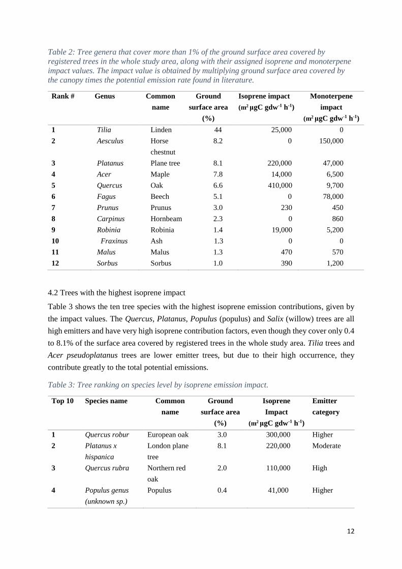
Table 2 shows the tree genera that are most abundant in the study area and that cover more than

one percent of the ground surface area covered by the canopy of registered trees. The isoprene

and monoterpene impact levels are also given. It shows that Tilia (linden) trees are by far the

most planted trees, with more than 44% being Tilia trees, including Tilia cordata, Tilia

platphyllos and Tilia x europaea. These three species are all low isoprene emitters and show no

monoterpene emissions. The second most abundant genus is Aesculus (horse chestnut), which

includes the species Aesculus carnea and Aesculus hippocastanum, with the latter one being

more abundant and taking up 7.8% of the tree cover (see Table 6 in appendix). Aesculus species

are high monoterpene emitters. Platanus (plane tree) trees make up over 8% of the tree cover

as well. The only Platanus species that is present in the study area is Platanus x hispanica, also

known as Platanus x acerifolia, and which contributes significantly to the isoprene and

monoterpene emissions. Next is the Acer (maple) genus, which includes Acer campestre, Acer

platanoides, Acer pseudoplatanus, Acer saccharinum and Acer x freemanii, which are low

isoprene and low monoterpene emitters. The genus taking up over 6% of the registered tree

cover is the Quercus (oak) genus, which summarizes species which can be high isoprene or

high monoterpene emitters, as well as a combination of both. In this study area, Quercus robur,

rubra, petraea and coccinea are significant isoprene emitters, as well as emitters of lower rates

of monoterpene, while Quercus cerris is a high monoterpene emitter only. The Fagus (beech)

genus combines Fagus sylvatica and Fagus orientalis, where Fagus orientalis does not emit

isoprene or monoterpene at all, whereas Fagus sylvatica is a high monoterpene emitter and is

responsible for the monoterpene impact of this genus. The Prunus (prunus) genus is a generally

low emitter and does not have a large contribution to BVOC emissions. The only tree belonging

to the Carpinus (hornbeam) genus in this study area is Carpinus betulus, which is low

monoterpene emitter. The Robinia genus, represented by Robinia pseudoacacia is an isoprene

and monoterpene emitter. Next, the Fraxinus (ash) genus, represented by Fraxinus angustifolia,

exselsior and ornus, which cover 1.3% of the area covered by registered trees, are non-emitting

trees. The Malus and Sorbus genera are also very low emitters of isoprene and monoterpene

and make up around 1% of the tree cover each.

12

Table 2: Tree genera that cover more than 1% of the ground surface area covered by

registered trees in the whole study area, along with their assigned isoprene and monoterpene

impact values. The impact value is obtained by multiplying ground surface area covered by

the canopy times the potential emission rate found in literature.

Rank # Genus Common

name

Ground

surface area

(%)

Isoprene impact

(m2 μgC gdw-1 h-1)

Monoterpene

impact

(m2 μgC gdw-1 h-1)

1

2

Tilia

Aesculus

Linden

Horse

chestnut

44

8.2

25,000

0

0

150,000

3 Platanus

Plane tree 8.1

220,000

47,000

4 Acer

Maple 7.8

14,000

6,500

5 Quercus Oak 6.6

410,000

9,700

6 Fagus

Beech 5.1

0

78,000

7 Prunus Prunus 3.0

230

450

8 Carpinus Hornbeam 2.3

0

860

9 Robinia Robinia 1.4

19,000

5,200

10

Fraxinus Ash 1.3 0

0

11 Malus Malus 1.3

470

570

12 Sorbus Sorbus 1.0 390

1,200

4.2 Trees with the highest isoprene impact

Table 3 shows the ten tree species with the highest isoprene emission contributions, given by

the impact values. The Quercus, Platanus, Populus (populus) and Salix (willow) trees are all

high emitters and have very high isoprene contribution factors, even though they cover only 0.4

to 8.1% of the surface area covered by registered trees in the whole study area. Tilia trees and

Acer pseudoplatanus trees are lower emitter trees, but due to their high occurrence, they

contribute greatly to the total potential emissions.

Table 3: Tree ranking on species level by isoprene emission impact.

Top 10 Species name Common

name

Ground

surface area

(%)

Isoprene

Impact

(m2 μgC gdw-1 h-1)

Emitter

category

1 Quercus robur European oak 3.0 300,000 Higher

2 Platanus x

hispanica

London plane

tree

8.1 220,000 Moderate

3 Quercus rubra Northern red

oak

2.0 110,000 High

4 Populus genus

(unknown sp.)

Populus 0.4 41,000 Higher

13

5 Salix x pendulina Weeping

willow

0.2 34,000 Highest

6 Populus x

canadensis

''Robusta''

Canadian

poplar

0.4 29,000 High

7 Tilia sp. Linden 44 25,000 Lower

8 Robinia

pseudoacacia

Black locust 1.4 19,000 Low

9 Salix alba White willow 0.4 18,000 High

10 Acer

pseudoplatanus

Sycamore

maple

4.4 13,000 Lower

Sum 65 810,00

4.3 Trees with the highest monoterpene impact

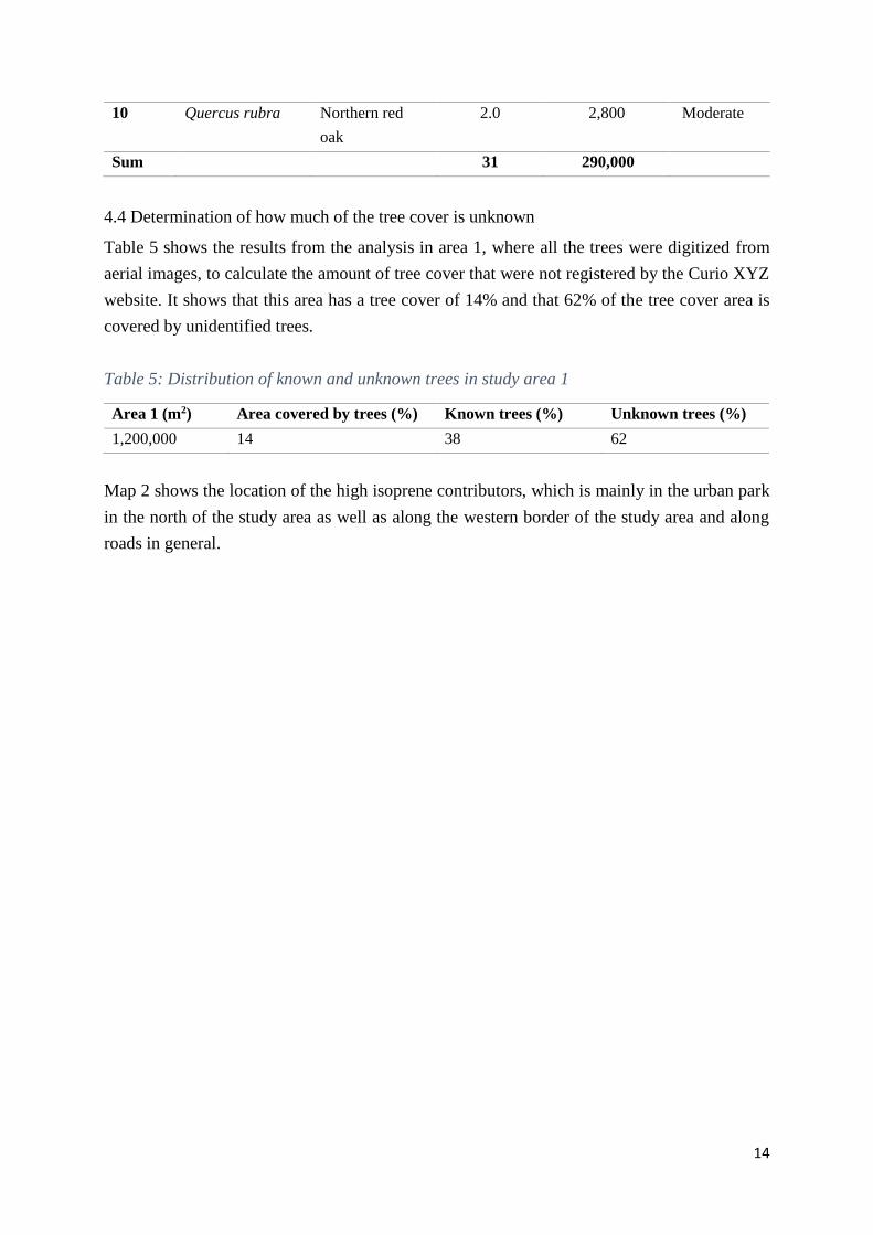
Table 4 lists the ten highest monoterpene emission contributors, with Aesculus hippocastanum

being the highest contributor with an impact value of 140,000 m2 μgC gdw-1 h-1 followed by

Fagus sylvatica and Platanus x hispanica. All trees in this ranking are very high emitters,

except for Acer pseudoplatanus and the Quercus trees, which are moderate and low emitters

but contribute greatly due to their abundant occurrence in the study area.

Table 4: Ranking on species level by monoterpene emission impact, along with the percentage

of ground surface area covered by tree canopies in the whole study area and the emission

categories of the species.

Top 10 Species Common name Ground

surface

area (%)

Monoterpene

Impact

(m2 μgC gdw-1 h-1)

Emitter

category

1 Aesculus

hippocastanum

Horse chestnut 7.8 140,000 Highest

2 Fagus sylvatica European beech 4.8 78,000 Highest

3 Platanus x

hispanica

London plane

tree

8.1 47,000 High

4 Aesculus carnea Red horse-

chestnut

0.4 7,000 Highest

5 Robinia

pseudoacacia

Black locust 1.4 5,200 High

6 Quercus cerris Turkey oak 1.5 4,000 Moderate

7 Acer

pseudoplatanus

Sycamore maple 4.4 3,300 Low

8 Magnolia sp. Magnolia 0.1 3,100 Highest

9 Ginko biloba Maidenhair tree 0.6 2,800 High

14

10 Quercus rubra Northern red

oak

2.0 2,800 Moderate

Sum 31 290,000

4.4 Determination of how much of the tree cover is unknown

Table 5 shows the results from the analysis in area 1, where all the trees were digitized from

aerial images, to calculate the amount of tree cover that were not registered by the Curio XYZ

website. It shows that this area has a tree cover of 14% and that 62% of the tree cover area is

covered by unidentified trees.

Table 5: Distribution of known and unknown trees in study area 1

Area 1 (m2) Area covered by trees (%) Known trees (%) Unknown trees (%)

1,200,000 14 38 62

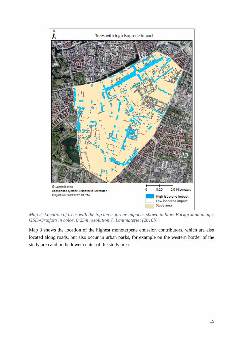
Map 2 shows the location of the high isoprene contributors, which is mainly in the urban park

in the north of the study area as well as along the western border of the study area and along

roads in general.

15

Map 2: Location of trees with the top ten isoprene impacts, shown in blue. Background image:

GSD-Ortofoto in color, 0.25m resolution © Lantmäteriet (2016b)

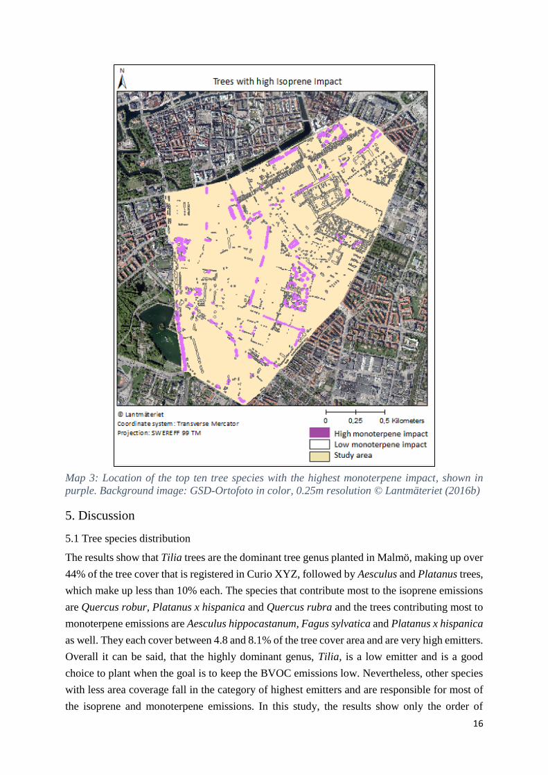
Map 3 shows the location of the highest monoterpene emission contributors, which are also

located along roads, but also occur in urban parks, for example on the western border of the

study area and in the lower center of the study area.

16

Map 3: Location of the top ten tree species with the highest monoterpene impact, shown in

purple. Background image: GSD-Ortofoto in color, 0.25m resolution © Lantmäteriet (2016b)

5. Discussion

5.1 Tree species distribution

The results show that Tilia trees are the dominant tree genus planted in Malmö, making up over

44% of the tree cover that is registered in Curio XYZ, followed by Aesculus and Platanus trees,

which make up less than 10% each. The species that contribute most to the isoprene emissions

are Quercus robur, Platanus x hispanica and Quercus rubra and the trees contributing most to

monoterpene emissions are Aesculus hippocastanum, Fagus sylvatica and Platanus x hispanica

as well. They each cover between 4.8 and 8.1% of the tree cover area and are very high emitters.

Overall it can be said, that the highly dominant genus, Tilia, is a low emitter and is a good

choice to plant when the goal is to keep the BVOC emissions low. Nevertheless, other species

with less area coverage fall in the category of highest emitters and are responsible for most of

the isoprene and monoterpene emissions. In this study, the results show only the order of

17

magnitude of the emission potential of the different tree species, as the emission rates were

taken from different literature sources, which comes with a variety of uncertainties.

5.2 Amount of unknown trees

The results given in Table 4 show that unknown and unregistered trees make up 62% of the tree

cover in study area 1. This is due to the two large cemeteries that are in the study area, S:t Pauli

Norra kyrkogård and S:t Pauli Mellersta kyrkogård, where very few or no trees at all are

identified. These two cemeteries are not the only two in Malmö that are not registered. In fact,

several other cemeteries like Gamla kyrkogården in the old town, parts of Slottsträdgården, all

Östra kyrkogården and its surroundings, as well as many street and garden trees are not

registered. This further demonstrates how high the uncertainty in the isoprene and monoterpene

emission impact is, when more than half of the tree cover is unknown and cannot be analyzed

with literature values.

5.3 Literature source uncertainties

5.3.1 Variation in emission rates of the same species

Firstly, the emission rates were taken from different sources, which are studies performed in

different parts of the world with different environmental conditions, as well as emission

inventories which assemble even more different sources. All the measured emission rates are

standardized to a PAR value of 1000 μmol m-2 s-1 and a temperature of 30°C using the Guenther

et al. algorithm (Guenther et al. 1993), but different growing conditions like soil moisture, air

pollution and eventual undetected diseases can influence the measured rates significantly

(Laothawornkitkul et al. 2009; Bäck et al. 2012). Furthermore, the age of the measured trees

and even the leaves or needles on the branch play a major role, as younger leaves and needles

show higher emission rates than older ones (Wang et al. 2017).

Secondly, some of the species found in the study area are not native to Europe and were only

analyzed by studies performed in their native environment, where the growing conditions might

be different. An example of this is Populus simonii, which is a native tree in northern China

(FAO 2002) and was analyzed in Yunmeng Mountain, Beijing in a study by Li et al. (2017),

where the growing conditions are different from the conditions in the urban area of Malmö. The

climate differs between the two locations, because the average temperature on Yunmeng

mountain is 25°C in July and -7 in January (Zhang and Shao 2015), while Malmö has an average

temperature of 17°C in July and 0°C in January (Climate-data.org 2019). Furthermore,

Yunmeng Mountian is affected by a summer monsoon from June to September, with most of

the precipitation falling in this time period, while Malmö experiences precipitation evenly over

the whole year. Both sites receive around 600-700mm of rain each year, but the difference in

distribution will have an impact on soil moisture throughout the year (Zhang and Shao 2015;

Climate-data.org 2019). As mentioned in the section 2.3, water stress and temperature can

affect BVOC emission rates.

18

Thirdly, another factor that influences the accuracy of the results is that some species were

assigned a high variation of emission rates by different literature sources. An example for this

is the species Quercus petraea, where the isoprene emission rates varies between 0.6 and 45

μgC gdw-1 h-1, depending on the source. Another example of a varying isoprene emission rate

is the Tilia genus, where Karl et al. (2009) state that Tilia species emit 0 μgC gdw-1 h-1, whereas

Owen et al. (2003) measured 5.5 μgC gdw-1 h-1. Since it is the most common species in Malmö,

this rate difference would make a large difference in the resulting overall emission. The same

phenomenon occurred for literature values of monoterpene emissions. One example is Fagus

sylvatica. Here, the literature values range from 0.5 to 21.1 μgC gdw-1 h-1, which is a huge range

from low to highest emitter, considering that this species makes up almost 5% of the tree cover.

For the impact calculations, averages were taken for all the species with varying values, in order

to account for the extreme range of values. Therefore, just from looking at the literature values,

the uncertainty in the accuracy of the results is already important.

5.3.2 Seasonal variations of emission rates

Another factor that impacts the accuracy of these results is stated by Benjamin et al. (1997),

who compiled an inventory of isoprene and monoterpene emission rates of trees and shrubs

found in the California South Coast Air Basin, and combined the hourly emission rates with

daily light intensity and temperature data to calculate daily emission rates. He found out that

the hourly emission rates given in most studies and inventories are an overestimation, since

they are usually measured around noon on a summer day, when emission rates are at their peak.

Through the standardization, diurnal variations in emission rates are taken into account, but

seasonal variations are left out. Therefore, they do not consider that emission rates might be

much lower during winter, when deciduous trees do not have leaves. Another seasonal impact

that affects emission rates is flowering, which was an outcome of the study conducted by Baghi

et al. (2012), which measured the BVOC emissions of different tree species during spring and

summer to determine if there are differences in emission rates during and after flowering. For

the species Aesculus hippocastanum, the results showed that the species had a monoterpene

emission rate of 9.1 μgC gdw-1 h-1 during flowering and a rate of 12 μgC gdw-1 h-1 after

flowering. Isoprene compounds were not found. This shows that is makes a big difference when

the measurements are taken. For other sources, no information was given on whether the

measured trees were flowering or not. For this study, the after-flowering value was taken, since

it would be valid for a longer period as the species is in bloom for around 2.5 weeks in mid-

May only. Most trees bloom in spring. Nevertheless, the majority of the literature sources

collected their data in the time period of June to October ((Benjamin and Winer 1997; Isebrands

et al. 1999; Curtis et al. 2014; Li et al. 2017). Only the study by Owen et al (2003) took

averages over the whole year and the other literature sources did not provide the dates of their

field data collection. Not only do these uncertainties and ranges in values influence the results,

but also not finding any reliable sources of BVOC emission for a species influences the total

emissions. This was the case for four species, Parrotia persica, which is native in northern Iran,

19

Phellodendron amurense, native in north-east Asia and Japan, Pterocarya fraxinifolia, which

is endemic in northern Turkey, Caucasus and northern Iran, and lastly Quercus macranthera,

which also comes from Caucasus and northern Iran (SKUD 2019).

5.4 Limitations of methodology: digitization

Not only do the literature sources affect the results, the methodology applied to calculate the

tree cover also comes with sources of error. In this study, the trees were digitized from

orthophotos and not regular aerial images. This had the result that some trees might not have

been visible due to being obstructed by buildings. This lowered the accuracy of digitizing the

actual tree cover when the tree was not visible but was indicated to be there by Curio XYZ. For

registered trees, this was accounted for by digitizing an estimation of where the tree would be,

but for unregistered trees, this led to an underestimation of tree cover. Furthermore, for the

unregistered tree cover, the orthoimages in RGB and IR with a resolution of 0.25m were not

always clear enough to determine if the vegetation was a tree or a small bush when there were

no shadows indicating its height. In addition, due to the large number of trees and the low

resolution, and many deciduous trees not having leaves at the time of when the orthophotos

were taken, the shape of the crown could not always be drawn with high accuracy. Another

factor that is not considered when only taking into account canopy cover to determine the

emission potential, is that tree species can have a large variety of canopy shapes. For example,

the Aesculus hippocastanum species grows a very wide round crown, whereas the Poplar

species grow high narrow crowns. Therefore, trees with wide and shallow crowns are

overestimated and trees with deep and narrow crowns are underestimated in this study and it

would have been necessary to look at leaf area indices of each species to correct for that. In

addition, this study did not look at tree age or tree health, which are both factors that affect

emission rates greatly (Wang et al. 2017). From the Curio XYZ website, it was apparent that a

lot of young trees were present in the study area, including high emitting species, that do not

contribute much to the tree cover area now, but are likely to do so in the future and probably

led to an underestimation of the emission impact by the tree cover, since younger trees often

have higher emission rates (Wang et al. 2017).

5.5 Strength of methodology: time efficiency

The methodology used in this study comes with many sources of errors and uncertainties, but

it is highly time efficient to determine the order of magnitude of the BVOC emission potential

of the urban trees in Malmö. The study area included 100 different species and it took around

16h of intense work to digitize the 3150 small polygons and to assign them their species. In

comparison, the height and diameter of 24 Aesculus hippocastanum trees were measured on

Södra Promenaden in Malmö, as well as 100 trees of differing species in Kungsgården and

around the old town, to calculate their leaf biomass with the use of allometric equations. These

equations use regression models between different parameters like tree height and diameter in

order to calculate the biomass of the tree. From the leaf biomass values and the standardized

20

BVOC emission rates found in literature, the total emissions of the trees can be obtained. Just

the tree measurements of those 124 trees took 48h of field work. This project was not finished,

due to the lack of allometric equations for each species, but it shows that the methodology used

in this study can cover a much larger area by using aerial images to determine canopy size and

area coverage by the different tree species, instead of measuring every single tree in the study

area.

5.6 Effect of BVOC lifetime in the atmosphere and local weather

This study determined the potential isoprene and monoterpene emissions impact on air quality

by the trees in the study area, but isoprene has a chemical lifetime of 50min to 1.5h, depending

on which chemical it reacts with in the atmosphere, and monoterpene has a lifetime of 5min to

5h, depending on the compound (Benjamin and Winer 1997). This means that the study did not

account for any BVOC emissions coming from the vegetation surrounding the study area and

this can be a major factor, since Pildammsparken is right on the western border of the study

area. Furthermore, the prevailing wind direction in Malmö is from the West, South-West, with

a wind speed of around 4.5m/s (Miljöförvaltningen 2018), so that the BVOC emissions from

Pildammsparken are very likely to enter the study area. Nevertheless, the ozone forming

reaction is slower than the emission rate, therefore the highest ozone levels are usually found

downwind of urban areas, in this case East of Malmö (Calfapietra et al. 2013). This is not only

an error source in this study, but it should also be considered by urban planners when they are

planning to plant trees in areas with higher air pollution.

5.7 Other effect of trees on urban areas: ecosystem services

Trees are not only known to contribute to aerosol and ozone formation, they also provide a

variety of positive aspects to the urban ecosystem. Some of these ecosystem services are for

example the removal of fine particulate matter (PM10 and PM2.5), the provision of surfaces

for water infiltration, the reduction of the urban heat island effect through evapotranspiration,

CO2 uptake, provision of shade and the provision of recreational value (Manes et al. 2016). All

of those are not taken into consideration and this study but would have to be included in order

to make a scientific and objective decision on the suitability of different tree species for the

urban environment.

5.8 Future studies

If this study could be repeated, then more variables would be taken into consideration when

calculating the emission impact that each specie has on the cities air quality. That would include

tree species’ leaf area index and tree age, and if possible, also tree health. If more time would

be available, then the extent of the study could be elaborated, and emission rates could be

measured in Malmö itself and then be compared to literature values.

21

6. Conclusion

In conclusion, the aim was achieved by

• Estimating the surface area that each tree species covers in the study area and by

multiplying that area with the standardized emission rates found in literature

• To answer the first research question on which species are present in the study area, the

study revealed that there are 100 different species in the study area and the most

common genus is Tilia, with 44% of the area covered by trees being covered by Tilia

trees. The Tilia genus is followed by the Aesculus and Platanus genera, with a coverage

of 8.2% and 8.1% of the tree cover area respectively.

• The second research question on which species contribute most to potential BVOC

emission can be answered by stating that it is not the most abundant species, the Tilia

species, but species that are less abundant but have higher potential emission rates. The

highest potential isoprene impact comes from Quercus robur with an impact value of

300,000 m2 μgC gdw-1 h-1. The highest monoterpene impact comes from Aesculus

hippocastanum with an impact value of 140,000 m2 μgC gdw-1 h-1. In comparison, Tilia

trees are low emitters of isoprene and non-emitters of monoterpene and therefore have

a low contribution to BVOC emissions in Malmö, with an isoprene impact value of

25,000 m2 μgC gdw-1 h-1.

• This study also revealed that there is a large discrepancy in literature emission rates for

the same species, which affected the accuracy and potentially also the magnitude of the

emission impact that the trees of the study area have on air quality. Due to the large

number of uncertainties, this study was not able to provide actual values of isoprene and

monoterpene emissions in the study area, but it provides an idea of the composition of

species and their estimated emission potential, which can be useful for urban planning

purposes.

22

7. Appendix

Table 6: List of the species occurring in the study area, along with their canopy area, standardized

isoprene and monoterpene emission rates and their impact values

Species Ground

surface

area

(m2)

Percentage of

total tree cover

area

(%)

Isoprene

emission

rate (μgC gdw-1 h-

1)

Monoterpene

emission rate (μgC gdw-1 h-1)

Avg.

ISP (μgC

gdw-1

h-1)

Avg.

MT (μgC

gdw-1

h-1)

Impact

ISP (m2

μgC

gdw-1

h-1)

Impact MT (m2

μgC

gdw-1

h-1)

Acer campestre 3,143 2.10 0.1c 0.5c 0.1 0.5 314 1,571

Acer platanoides 1,398 0.93 0.1c; 0.4a 0.5c; naa 0.25 0.5 350 699

Acer pseudoplatanus 6,547 4.38 0.1c; 3.9f 0.5c 2 0.5 13,094 3,273

Acer saccharinum 463 0.31 N/Aa; 0.1c 2.2/3.5a; 0.5c 0.1 2.1 46 957

Acer x freemanii 27 0.02 0.1c 0.5c 0.1 0.5 3 13

Aesculus carnea 586 0.39 0d 12d 0 12 0 7,031

Aesculus hippocastanum 11,679 7.81 0d 12d 0 12 0 140,151

Ailanthus altissima 555 0.37 0.1g 1.6g 0.1 1.6 56 888

Alnus cordata 296 0.20 0c 1.5c 0 1.5 0 444

Alnus glutinosa 36 0.02 0c 1.5c 0 1.5 0 54

Alnus incana 605 0.40 0c 1.5c 0 1.5 0 908

Amelanchier lamarckii 11 0.01 0g, h 0g, h 0 0 0 0

Araucaria araucana 64 0.04 0.1g 1.5g 0.1 1.5 6 96

Betula dalecarlica e 83 0.06 0c 3c 0 3 0 249

Betula pendula 908 0.61 0a; 0c;

0.05f

0.19/5.4a; 3c;

2.63f

0.02 2.8 15 2,547

Betula pubescens 188 0.13 0c 3c 0 3 0 564

Buxus sempervirens 150 0.10 10c 0.2c 10 0.2 1505 30

Carpinus betulus 3,447 2.30 0a; 0c 0.4a; 0.1c 0 0.25 0 862

Castanea sativa 257 0.17 0c 10c 0 10 0 2,574

Catalpa bignonioides 33 0.02 0a 0a 0 0 0 0

Catalpa sp. 105 0.07 0a 0a 0 0 0 0

Cedrus deodara 17 0.01 0c 1c 0 1 0 17

Celtis occidentalis 40 0.03 0.1g 0.2g 0.1 0.2 4 8

Cercidiphyllum japonicum 158 0.11 39.4g 1.6g 39.4 1.6 6238 253

Cornus mas 278 0.19 0.1g 1.6g 0.1 1.6 28 446

Corylus colurna 67 0.04 0c 0c 0 0 0 0

Crataegus intricata 515.39 0.34 0g 0g 0 0 0 0

Crataegus laevigata 13 0.01 0g 0g 0 0 0 0

Crataegus monogyna 469 0.31 0.03f 0.88f 0.03 0.88 14 413

Crataegus punctata 133 0.09 0g 0g 0 0 0 0

Crataegus rhipidophylla 42 0.03 0g 0g 0 0 0 0

Crataegus x lavallei 89 0.06 0g 0g 0 0 0 0

Fagus orientalis 371 0.25 0c 0c 0 0 0 0

Fagus sylvatica 7,224 4.83 0a, c 0.5a; 21.1c 0 10.8 0 78,023 0

Fraxinus angustifolia 460 0.31 0c 0c 0 0 0 0

23

Fraxinus excelsior 1,456 0.97 0c, f 0c, f 0 0 0 0

Fraxinus ornus 59 0.04 0c 0c 0 0 0 0

Ginkgo biloba 931 0.62 0a 3a 0 3 0 2,793

Gleditsia triacanthos 828 0.55 0.1g 1.2d; 0.2g 0.1 0.7 83 579

Juglans regia 202 0.14 0c 1c 0 1 0 202

Juniperus sp. 75 0.05 0c 0c 0 0 0 0

Koelreuteria paniculata 244 0.16 44.9g 0g 44.9 0 10,953 0

Laburnum x watereri

''Vossii"

45 0.03 0.1g 0.2g 0.1 0.2 5 9

Larix decidua 156 0.10 0c 5c 0 5 0 781

Liquidambar styraciflua 143 0.10 34/63-99a 3.5/ N/Aa 57.5 3.5 8,246 502

Liriodendron tulipifera 65 0.04 4.1a N/Aa 4.1

266 0

Magnolia 79 0.05 Naa, h; 0.1g 5.9a; 3g; 107h 0.1 39 8 3,058

Magnolia x soulangeana 66 0.04 Naa, h; 0.1g 5.9a; 3g; 107h 0.1 39 7 2557

Malus sp. 853 0.57 0c; 0.5f 0c; 0.6f 0.25 0.3 213 256

Malus baccata 308 0.21 0c; 0.5f 0c; 0.6f 0.25 0.3 77 92

Malus domestica 75 0.05 0c; 0.5f 0c; 0.6f 0.25 0.3 19 23

Malus floribunda 537 0.36 0c; 0.5f 0c; 0.6f 0.25 0.3 134 161

Malus x purpurea 113 0.08 0c; 0.5f 0c; 0.6f 0.25 0.3 28 34

Metasequoia

glyptostroboides

367 0.25 0g 3g 0.25 0.3 92 110

Morus alba 31 0.02 0.1g 0.2g 0.1 0.2 3 6

Parrotia persic 46 0.03 N/A N/A

0 0

Phellodendron amurense 197 0.13 N/A N/A

0 0

Pinus heldreichii 32 0.02 0c 3c 0 3 0 95

Pinus nigra 165 0.11 0c 3c 0 3 0 495

Platanus x hispanica 12,113 8.10 18.5c 0.1c; 3.9h 18.5 3.9 22,4095 47,242

Populus simonii 252 0.17 46.9j 03; N/Aj 46.9 0 11,827 0

Populus sp. 588 0.39 51-100a;

60/70c;

70g

0-4.5a; 0c; 0.1g 70 1.15 41,289 677

Populus tremula 30 0.02 51a 4.6a 51 4.6 1,521 137

Populus x canadensis

''Robusta''

639 0.43 N/Ac; 46i 0c; N/Ai 46 0 29,383

Prunus 1,199 0.80 0c; 0.1f 0.1c; 0.13f 0.05 0.1 60 0

Prunus avium 1,549 1.04 0c; 0.1f 0.1c; 0.13f 0.05 0.1 77 120

Prunus cerasifera 563 0.38 0c; 0.1f 0.1c; 0.13f 0.05 0.1 28 155

Prunus padus 255 0.17 0c; 0.1f 0.1c; 0.13f 0.05 0.1 13 56

Prunus sargentii 617 0.41 0c; 0.1f 0.1c; 0.13f 0.05 0.1 31 25

Prunus serrula 206 0.14 0c; 0.1f 0.1c; 0.13f 0.05 0.1 10 62

Prunus virginiana

''Shubert''

26 0.02 0c; 0.1f 0.1c; 0.13f 0.05 0.1 1 21

Prunus x persicoides 93 0.06 0c; 0.1f 0.1c; 0.13f 0.05 0.1 5 3

Pterocarya fraxinifolia 813 0.54 N/A N/A N/A N/A N/A 9

Pyrus calleryana 95 0.06 0c, e 0c, e 0 0 0

Pyrus communis 78 0.05 0c 0c 0 0 0 N/A

Quercus cerris 2,183 1.46 0a, c 3.1a; 0.6c 0 1.85 0 0

Quercus coccinea 220 0.15 20.1a 3.2a 20.1 3.2 4419 0

24

Quercus macranthera 103 0.07 N/A N/A N/A N/A N/A 4,038

Quercus petraea 13 0.01 0.61k; 45c 0.12k; 0.3c 22.805 0.21 303 704

Quercus robur 4,442 2.97 76.6a; 45-

61a; 70c

0a; 1c 67 0.5 295,554 N/A

Quercus rubra 2,920 1.95 14.8a; 45-

61a; 35c

1.8a; 0.1c 39 0.95 113,894 3

Rhamnus cathartica 19 0.01 36.9g 0g 36.9 0 691 2,221

Robinia pseudoacacia 2,111 1.41 1.10a;

13.5a; 12c;

N/Ah

0a; 4.7a; 0.1c;

5.1h

8.9 2.5 18,719 2,774

Salix 29 0.02 22.7f 1f 22.7 1 661 0

Salix alba 591 0.40 37.2c;

22.7f

1.1c; 1f 30 1 17,708 5,225

Salix x pendulina 300 0.20 115a* N/Aa* 115 N/A 34,486 29

Salix x sepulcralis 296 0.20 28c 0.8c 28 0.8 8,283 591

Sambucus nigra 47 0.03 0e 0e 0 0 0 0

Sorbus 14 0.01 0c; 0.5f 0c; 1.5f 0.25 0.75 4 237

Sorbus aria 172 0.12 0c; 0.5f 0c; 1.5f 0.25 0.75 43 0

Sorbus aucuparia 49 0.03 0c; 0.5f 0c; 1.5f 0.25 0.75 12 11

Sorbus decora 235 0.16 0c; 0.5f 0c; 1.5f 0.25 0.75 59 129

Sorbus intermedia 1,060 0.71 0c; 0.5f 0c; 1.5f 0.25 0.75 265 37

'Sorbus x thuringiaca 26 0.02 0c; 0.5f 0c; 1.5f 0.25 0.75 6 177

Styphnolobium japonicum 891 0.60 N/A N/A

795

Taxus baccata 813 0.54 N/Ah 1.1h N/A 1.1 0 19

Tilia sp. 8,915 5.96 0c; 5.5f 0c, f 2.75 0 24,518 0

Tilia cordata 4,930 3.30 0b, c 0.7b; 0c 0 0 0 894

Tilia platyphyllos 554 0.37 0c 0c 0 0 0 3,501 Tilia x europaea 51,999 34.76 0c 0c 0 0 0 0

Unknown trees 122,866

Gone trees 436

Sum known trees 149,583 100 869,768

323,717

References: a: Kesselmeier and Staudt 1999. a*: the value of Salix babylonica was taken,

since Salix x pendulina is a hybrid of Salix babylonica and either S. fragilis or S. euxina. For

the latter species, no literature values were found. b: Curtis et al. 2014. c: Karl et al. 2009.

d: Baghi et al. 2012. e: Benjamin and Winer 1997. f: Owen et al. 2003. g: Nowak et al. 2002.

This source provides isoprene and monoterpene emission rates on a genus level. h: Noe et al.

2008. i: Isebrands et al. 1999. j: Li et al. 2017. k: König et al. 1995.

25

8. References

Acosta Navarro, J. C., S. Smolander, H. Struthers, E. Zorita, A. M. Ekman, J. O. Kaplan, A.

Guenther, A. Arneth, et al. 2014. Global emissions of terpenoid VOCs from terrestrial

vegetation in the last millennium. J Geophys Res Atmos, 119: 6867-6885. DOI:

10.1002/2013JD021238

Bäck, J., J. Aalto, M. Henriksson, H. Hakola, Q. He, and M. Boy. 2012. Chemodiversity of a

Scots pine stand and implications for terpene air concentrations. Biogeosciences, 9: 689-

702. DOI: 10.5194/bg-9-689-2012

Baghi, R., D. Helmig, A. Guenther, T. Duhl, and R. Daly. 2012. Contribution of flowering trees

to urban atmospheric biogenic volatile organic compound emissions. Biogeosciences,

9: 3777-3785. DOI: 10.5194/bg-9-3777-2012

Benjamin, M. T., and A. M. Winer. 1997. Estimating the ozone-forming potential of urban trees

and shrubs. Atmospheric Environment, 32: 53-68. DOI: https://doi.org/10.1016/S1352-

2310(97)00176-3

Berg, A. R., C. L. Heald, K. E. Huff Hartz, A. G. Hallar, A. J. H. Meddens, J. A. Hicke, J. F.

Lamarque, and S. Tilmes. 2013. The impact of bark beetle infestations on monoterpene

emissions and secondary organic aerosol formation in western North America.

Atmospheric Chemistry and Physics, 13: 3149-3161. DOI: 10.5194/acp-13-3149-2013

Bolsoni, V. P., D. P. de Oliveira, G. d. S. Pedrosa, and S. R. de Souza. 2018. Volatile organic

compounds (VOC) variation in Croton floribundus (L.) Spreng. related to

environmental conditions and ozone concentration in an urban forest of the city of Sao

Paulo, Sao Paulo State, Brazil. Hoehnea, 45: 184-191. DOI: 10.1590/2236-8906-

60/2017

Boucher, O., D. Randall, P. Artaxo, C. Bretherton, G. Feingold, P. Forster, V.-M. Kerminen,

Y. Kondo, et al., 2013. Clouds and Aerosols. Report, Cambridge, United Kingdom and

New York, NY, USA, 571-657 pp.

Breadboard Labs. 2019. Curio XYZ. Retrieved 19th April 2019, from

https://www.curio.xyz/world/tagged-

trees/overview?lat=55.59202136733458&lng=13.01674621730081&zml=15

Cahill, T., V. Seaman, M. J. Charles, R. Holzinger, and A. Goldstein. 2006. Secondary organic

aerosols formed from oxidation of biogenic volatile organic compounds in the Sierra

Nevada Mountains of California. Journal of Geophysical Research, 111. DOI:

10.1029/2006jd007178

Calfapietra, C., S. Fares, F. Manes, A. Morani, G. Sgrigna, and F. Loreto. 2013. Role of

Biogenic Volatile Organic Compounds (BVOC) emitted by urban trees on ozone

concentration in cities: A review. Environmental Pollution, 183: 71-80. DOI:

10.1016/j.envpol.2013.03.012

Climate-data.org. 2019. Klimat: Malmö. Retrieved 27th May 2019, from https://sv.climate-

data.org/europa/sverige/skane-laen/malmoe-382/.

Curtis, A. J., D. Helmig, C. Baroch, R. Daly, and S. Davis. 2014. Biogenic volatile organic

compound emissions from nine tree species used in an urban tree-planting program.

Atmospheric Environment, 95: 634-643. DOI: 10.1016/j.atmosenv.2014.06.035

Dindorf, T., U. Kuhn, L. Ganzeveld, G. Schebeske, P. Ciccioli, C. Holzke, R. Köble, G. Seufert,

et al. 2006. Significant light and temperature dependent monoterpene emissions from

European beech (Fagus sylvatica L.) and their potential impact on the European volatile

organic compound budget. Journal of Geophysical Research, 111. DOI:

10.1029/2005jd006751

26

EEA. 2018. Emissions of the main air pollutants in Europe. Retrieved 22 April 2019 2019, from

https://www.eea.europa.eu/data-and-maps/indicators/main-anthropogenic-air-

pollutant-emissions/assessment-4.

FAO. 2002. Technical Project Review Document (1991-2002), Project "Afforestation, Forestry

Research, Planning and Development in the Three North Region of China". Retrieved

20th May 2019, from http://www.fao.org/3/AC613E/AC613E02.htm.

Ghirardo, A., K. Koch, R. Taipale, I. Zimmer, J. P. Schnitzler, and J. Rinne. 2010.

Determination of de novo and pool emissions of terpenes from four common

boreal/alpine trees by CO2 labelling and PTR-MS analysis. Plant, Cell and

Environment, 33: 781-792. DOI: 10.1111/j.1365-3040.2009.02104.x

The World Bank Group.2018a. Urban population (% of total). Retrieved 27th May 2019, from

https://data.worldbank.org/indicator/sp.urb.totl.in.zs .

The World Bank Group. 2018b. Urban population growth (annual %). Retrieved 27th May, from

https://data.worldbank.org/indicator/SP.URB.GROW?locations=1W&most_recent_ye

ar_desc=false.

Guenther, A., C. N. Hewitt, D. Erickson, R. Fall, C. Geron, T. Graedel, P. Harley, L. Klinger,

et al. 1995. A global model of natural volatile organic compound emissions. Journal of

Geophysical Research 100: 8873-8892. DOI: 10.1029/94JD02950

Guenther, A., P. Zimmermann, and P. Harley. 1993. Isoprene and Monoterpene Emission Rate

Variability: Model Evaluations and Sensitivity Analyses. Journal of Geophysical

Research, 98: 12609-12617. DOI: 10.1029/93JD00527

Isebrands, J. G., A. B. Guenther, P. Harley, D. Helmig, L. Klinger, L. Vierling, P. Zimmermann,

and C. Geron. 1999. Volatile organic compound emission rates from mixed deciduous

and coniferous forests in Northern Wisconsin, USA. Atmospheric Environment, 33:

2527-2536.

Karl, M., A. Guenther, R. Köble, A. Leip, and G. Seufert. 2009. A new European plant-specific

emission inventory of biogenic volatile organic compounds for use in atmospheric

transport models. Biogeosciences, 6: 1059-1087.

Kesselmeier, J., and M. Staudt. 1999. Biogenic Volatile Organic Compounds (VOC): An

Overview on Emission, Physiology and Ecology. Journal of Atmospheric Chemistry,

33: 23-88. DOI: 10.1023/a:1006127516791

Kirkwood, R., and A. Longley. 2012. Clean Technology and the Environment. Springer Science

& Business Media.

Knudsen, J., R. Eriksson, J. Gershenzon, and B. Ståhl. 2006. Diversity and Distribution of Floral

Scent. The Botanical Review, 72: 1-120. DOI: 10.1663/0006-

8101(2006)72[1:Dadofs]2.0.Co;2

König, G., M. Brunda, H. Puxbaum, C. N. Hewitt, S. C. Duckham, and J. Rudolph. 1995.

Relative contribution of oxygenated hydrocarbons to the total biogenic VOC emissions

of selected mid-European agricultural and natural plant species. Atmospheric

Environment, 29: 861–874.

Kuhn, U., S. Rottenberger, T. Biesenthal, A. Wolf, G. Schebeske, P. Ciccioli, E. Brancaleoni,

M. Frattoni, et al. 2002. Isoprene and monoterpene emissions of Amazônian tree species

during the wet season: Direct and indirect investigations on controlling environmental

functions. Journal of Geophysical Research, 107. DOI: 10.1029/2001jd000978

Lahr, E., G. Schade, C. Crossett, and M. Watson. 2015. Photosynthesis and isoprene emission

from trees along an urban-rural gradient in Texas. Global Change Biology, 21: 4221-

4236. DOI: 10.1111/gcb.13010

Lantmäteriet. 2015. GSD-Vägkartan. Geodataportalen.

Lantmäteriet. 2016a. GSD-OrtofotoIR25. Geodataportalen.

Lantmäteriet. 2016b. GSD-OrtofotoRGB25. Geodataportalen.

Lantmäteriet. 2018. GSD-Fastighetskartan Bebyggelse. Geodataportalen.

27

Laothawornkitkul, J., J. E. Taylor, N. D. Paul, and C. N. Hewitt. 2009. Biogenic volatile organic

compounds in the Earth system. New Phytol, 183: 27-51. DOI: 10.1111/j.1469-

8137.2009.02859.x

Lelieveld, J., J. S. Evans, M. Fnais, D. Giannadaki, and A. Pozzer. 2015. The contribution of

outdoor air pollution sources to premature mortality on a global scale. Nature, 525: 367-

371. DOI: 10.1038/nature15371

Li, L., Y. Li, and S. Xie. 2017. A statistical approach for estimating representative emission

rates of biogenic volatile organic compounds and their determination for 192 plant

species/genera in China. Atmospheric Chemistry and Physics Discussions: 1-36. DOI:

10.5194/acp-2016-1116

Manes, F., F. Marando, G. Capotorti, C. Blasi, E. Salvatori, L. Fusaro, L. Ciancarella, M.

Mircea, et al. 2016. Regulating Ecosystem Services of forests in ten Italian Metropolitan

Cities: Air quality improvement by PM10 and O-3 removal. Ecological Indicators, 67:

425-440. DOI: 10.1016/j.ecolind.2016.03.009

Miljöförvaltningen, 2018. Luften i Malmö 2017. Malmö Stad, Report 1400-4690. [in Swedish,

English summary]

Noe, S. M., J. Penuelas, and U. Niinemets. 2008. Monoterpene emissions from ornamental trees

in urban areas: a case study of Barcelona, Spain. Plant Biology 10: 163-169. DOI:

10.1111/j.1438-8677.2007.00014.x

Nowak, D., D. Crane, J. Stevens, and M. Ibarra, 2002. Brooklyn’s Urban Forest. Report NE-

29050-53 pp.

Owen, S. M., A. R. Mackenzie, H. Stewart, R. Donovan, and C. N. Hewitt. 2003. Biogenic

volatile organic compound (VOC) emission estimates from an urban tree canopy.

Ecological Applications, 13: 927-938.

Penuelas, J., and M. Staudt. 2010. BVOCs and global change. Trends in Plant Science, 15: 133-

144. DOI: 10.1016/j.tplants.2009.12.005

Seyyednejad, S. M., M. Niknejad, and H. Koochak. 2011. A Review of Some Different Effects

of Air Pollution on Plants. Research Journal of Environmental Sciences, 5: 302-309.

DOI: 10.3923/rjes.2011.302.309

Simon, H., J. Fallmann, T. Kropp, H. Tost, and M. Bruse. 2019. Urban Trees and Their Impact

on Local Ozone Concentration—A Microclimate Modeling Study. Atmosphere, 10.

DOI: 10.3390/atmos10030154

SKUD. 2019. Svensk Kulturväxtdatabas Retrieved 20th May 2019, from

https://www.slu.se/centrumbildningar-och-projekt/skud/vaxtnamn/.

Malmö Stad. 2019. Malmö - Sveriges snabbast växande storstad. Retrieved 27th May 2019,

from https://malmo.se/Service/Om-Malmo-stad/Demokrati-beslut-och-

paverkan/Fakta-och-statistik/Befolkning/Befolkningstillvaxt.html.

Tang, J., G. Schurgers, H. Valolahti, P. Faubert, P. Tiiva, A. Michelsen, and R. Rinnan. 2016.

Challenges in modelling isoprene and monoterpene emission dynamics of Arctic plants:

a case study from a subarctic tundra heath. Biogeosciences, 13: 6651-6667. DOI:

10.5194/bg-13-6651-2016

Wang, M., G. Schurgers, A. Arneth, A. Ekberg, and T. Holst. 2017. Seasonal variation in

biogenic volatile organic compound (BVOC) emissions from Norway spruce in a

Swedish boreal forest. Boreal Environment Research, 22: 353-367.

Zemankova, K., and J. Brechler. 2010. Emissions of biogenic VOC from forest ecosystems in

central Europe: estimation and comparison with anthropogenic emission inventory.

Environmental Pollution, 158: 462-469. DOI: 10.1016/j.envpol.2009.08.032

Zhang, J.-T., and D. Shao. 2015. Attributes of Forest Diversity in the Yunmeng Mountain

National Forest Park in Beijing, China. Applied Ecology and Environmental Research,

13. DOI: 10.15666/aeer/1303_769782

28

Zimmer, W., N. Brüggemann, S. Emeis, C. Giersch, A. Lehning, R. Steinbrecher, and J. P.

Schnitzler. 2001. Process‐based modelling of isoprene emission by oak leaves. Plant,

Cell & Environment, 23: 585-595. DOI: 10.1046/j.1365-3040.2000.00578.x