ESTIMATION OF THE TERM PREMIUM

WITHIN AUSTRALIAN TREASURY BONDS

Fraser Jennison1

Australian Office of Financial Management Working Paper

2

2017-01

Date created: March 2017

Date modified: March 2017

1 Portfolio Strategy and Research, Australian Office of Financial Management, Treasury Building,

Langton Crescent, Parkes ACT 2600, Australia. The author is grateful for the interest, insights and comments

provided by Michael Bath, Philip Drummond, Richard Finlay, Angelia Grant, Leo Krippner,

Timothy McLennan-Smith and Matthew Wheadon. Thank you to Theodore Golat for assisting with initial work on

this topic and to the authors of Pricing the term structure with linear regressions: Tobias Adrian, Richard Crump

and Emmanuel Moench for providing useful code.

2 The views expressed in this paper are those of the authors and do not necessarily reflect those of the Australian

Office of Financial Management (AOFM) or the Australian Government.

© Commonwealth of Australia 2017

ISBN 978-1-925504-36-1

This publication is available for your use under a Creative Commons BY Attribution 3.0 Australia licence, with the exception of the Commonwealth Coat of Arms, the AOFM logo, photographs,

images, signatures and where otherwise stated. The full licence terms are available from http://creativecommons.org/licenses/by/3.0/au/legalcode.

Use of AOFM material under a Creative Commons BY Attribution 3.0 Australia licence requires you

to attribute the work (but not in any way that suggests that the AOFM endorses you or your use of

the work).

AOFM material used 'as supplied'

Provided you have not modified or transformed AOFM material in any way including, for example,

by changing the AOFM text; calculating percentage changes; graphing or charting data; or deriving

new statistics from published AOFM statistics — then AOFM prefers the following attribution:

Source: The Australian Office of Financial Management

Derivative material

If you have modified or transformed AOFM material, or derived new material from those of the

AOFM in any way, then AOFM prefers the following attribution:

Based on Australian Office of Financial Management data

Use of the Coat of Arms

The terms under which the Coat of Arms can be used are set out on the It’s an Honour website

(see www.itsanhonour.gov.au)

Other uses

Enquiries regarding this licence and any other use of this document are welcome at:

Communications Officer

Australian Office of Financial Management

Treasury Building, Langton Crescent

Parkes ACT 2600

Email: enquiries@aofm.gov.au

Estimation of the term premium within Australian Treasury Bonds

Fraser Jennison

2017-01

March 2017

ABSTRACT

We explore a linear-regression based dynamic term structure model developed by Adrian,

Crump and Moench ‘ACM’ (2013). We fit this model to the Australian Treasury Bond term structure

and estimate term premium through a daily yield decomposition. While our estimation approach

follows ACM, we consider an alternative estimation approach that corrects for the potential bias

inherent within a vector autoregressive system when variables are highly persistent. Our findings

show that this alternative specification leads to meaningfully different term premium estimations and

more variability in risk-neutral yields, while both estimation techniques suggest that the secular

decline in yields experienced within Australia has primarily been driven by a falling term premium.

To address estimation uncertainty, we provide yield decompositions with and without this alternative

estimation approach and suggest that the true data generating process most likely lies somewhere

within the bounds of these model specifications.

Portfolio Strategy and Research

The Australian Office of Financial Management

Treasury Building, Langton Crescent

Parkes ACT 2600

4

1. INTRODUCTION

Once found primarily within academic literature, the term premium has become a more widely

discussed concept. Representing the excess return investors demand for holding a longer-term

bond as opposed to investing in a series of short term bonds, this concept has materialised in many

settings including sovereign debt management, economic forecasting, and within central bank policy

discussions, particularly in relation to quantitative easing programs. To measure the term premium,

government bond yields need to be decomposed into two components: (1) a component based on

the expected future path of short term rates; and (2) a term premium component. As market

expectations are not directly observable,3 econometric techniques are required to separate the term

premium from expectations.

For robust term premium estimation, an econometric model that estimates a time-varying term

premium based on multiple dimensions of the yield curve is required. Campbell and Shiller (1988)

found evidence that rejects a time-invariant term premium, making static risk premia estimation

approaches such as the Fama MacBeth (1973) regression technique unfeasible in this context. In

the early bodies of literature, such as Vasicek (1977) or Cox, Ingersoll and Ross (1985), the

evolution of interest rates is explained by movements in the instantaneous spot rate. While

specifying a single factor model has the advantage of simplicity, information encapsulated within the

entirety of the yield curve is absent. More recent models reduce the yield curve into multiple factors,

whether these are latent variables extracted from the Nelson Siegel (1987) functional form or

through principal component analysis. While multi-factor models can accurately capture yield

dynamics, they may require computationally challenging non-linear cross-sectional restrictions

which may in themselves be problematic.4 Adrian, Crump and Moench ‘ACM’ (2013) propose a

multi-factor affine dynamic term structure model (DTSM) with coefficient estimation through a series

of linear-regressions. This approach can estimate a time-varying term premium, based on multiple

factors, without imposing non-linear restrictions using a three-step linear regression approach.

3 While financial participant surveys can be considered direct measures of expectations, survey based measures

are imperfect. Imperfections include the forecasts of participants not necessarily representing market-wide

interest rate expectations captured within the prices of instruments such as government bonds. Moreover,

surveys may be prone to a lack of incentive or the wrong incentive which may lead to a misrepresentation of

views (Kim and Orphanides 2005). Another (imperfect) measure of expectations includes direct inference from

instruments such as overnight indexed swaps. As with government bonds, these instruments include a term

premium component (Krippner and Callaghan 2016).

4 Hamilton and Wu (2010) detail the experience of those who have used these models and the significant

numerical challenges that arise with the estimation of non-linear likelihood surfaces. In particular, the potential for

parameter estimation not converging to the global maximum of the likelihood function is problematic.

5

Preceding ACM, seminal literature such as Duffie and Kan (1996), Dai and Singleton (2002),

Duffee (2002) and Kim and Wright (2005) have made contributions to the development of

multifactor-affine DTSM models. Within an Australian context: Finlay and Chambers (2009) fit a

term structure model to the Australian yield curve, Finlay and Wende (2011) fit a term structure

model to Australian Indexed bond yields and Wright (2011) includes Australia in an international

term premia empirical study. While DTSMs allow for decomposition of yields into a term premium

and a risk-neutral yield component5 that represents expectations for inflation and real yields,

estimation difficulties can arise. For example, it is known that parameter estimation within the vector

autoregressive system that represents interest rate dynamics can be difficult to identify. This

identification problem can cause a decomposition of yields to suffer from a bias if estimated through

a technique such as ordinary least squares (Bauer et al., ‘BRW’, 2012). This potential bias is a

function of the persistent nature of interest rates (slow-mean reversion) and the sample size of data

available (number of interest rate cycles captured). To account for this, BRW suggest that the

ordinary least squares VAR parameters within a DTSM should be bias-corrected which usually

results in estimated risk-neutral rates exhibiting more variability (greater persistency). Overall,

making a bias-correction within a DTSM typically leads to more variation in estimates of risk-neutral

yields and consequently more stable estimates of term premia.

This paper decomposes the Australian Treasury Bond yield curve in order to estimate the term

premium using the linear-regression based approach developed by Adrian, Crump and

Moench (2013). While our estimation approach follows ACM, we recognise the uncertainty around

estimation of the vector autoregressive system that ultimately represents interest rate dynamics in a

DTSM. As such, we provide two yield decompositions: (1) leaving the OLS VAR parameters

unadjusted as per ACM; and (2) using a bias-correcting technique to adjust the VAR parameters for

potential bias. We suggest that given estimation uncertainty, the true data-generating process most

likely lies somewhere within these model specifications. While this paper does not suggest an

optimal estimation approach, we do suggest that development of an optimisation procedure in order

to find a preferred combination of these alternative approaches could be valuable in managing the

uncertainty of DTSM coefficient estimations and consequently, term premium estimation.

In Section 2 we provide an overview of the ACM model, introduce the regressions used for

estimation and the data used for decomposing the Australian Treasury Bond term structure.

Section 3 discusses a potential issue of DTSM parameter estimation as a consequence of the

persistency of interest rates, proposing a technique to address this concern. Section 4 analyses the

optimal number of factors to include in this model. Section 5 explores model results and Section 6

concludes.

2. THE MODEL

The method we use to decompose the Australian Treasury Bond term structure is the linear

regressions approach presented by Adrian, Crump and Moench (2013). An overview of the model is

presented in this section; for more detail see ACM.

5 Risk-neutral in this context and throughout the paper refers to yields that would exist under the pure expectation

hypothesis. That is yields with no price of risk (term premium).

6

2.1 EXPRESSION

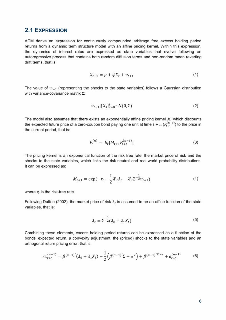
ACM derive an expression for continuously compounded arbitrage free excess holding period

returns from a dynamic term structure model with an affine pricing kernel. Within this expression,

the dynamics of interest rates are expressed as state variables that evolve following an

autoregressive process that contains both random diffusion terms and non-random mean reverting

drift terms, that is:

(1)

The value of (representing the shocks to the state variables) follows a Gaussian distribution

with variance-covariance matrix :

{ }

(2)

The model also assumes that there exists an exponentially affine pricing kernel which discounts

the expected future price of a zero-coupon bond paying one unit at time (

) to the price in

the current period, that is:

(3)

The pricing kernel is an exponential function of the risk free rate, the market price of risk and the

shocks to the state variables, which links the risk-neutral and real-world probability distributions.

It can be expressed as:

(4)

where is the risk-free rate.

Following Duffee (2002), the market price of risk is assumed to be an affine function of the state

variables, that is:

(5)

Combining these elements, excess holding period returns can be expressed as a function of the

bonds’ expected return, a convexity adjustment, the (priced) shocks to the state variables and an

orthogonal return pricing error, that is:

( )

(6)

7

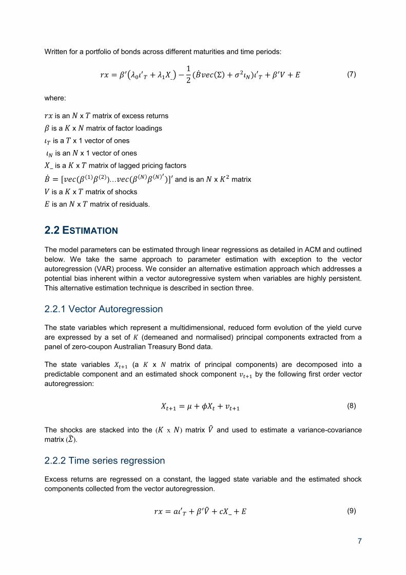
Written for a portfolio of bonds across different maturities and time periods:

(

)

(7)

where:

is an x matrix of excess returns

is a x matrix of factor loadings

is a x 1 vector of ones

is an x 1 vector of ones

is a x matrix of lagged pricing factors

)… and is an x matrix

is a x matrix of shocks

is an x matrix of residuals.

2.2 ESTIMATION

The model parameters can be estimated through linear regressions as detailed in ACM and outlined

below. We take the same approach to parameter estimation with exception to the vector

autoregression (VAR) process. We consider an alternative estimation approach which addresses a

potential bias inherent within a vector autoregressive system when variables are highly persistent.

This alternative estimation technique is described in section three.

2.2.1 Vector Autoregression

The state variables which represent a multidimensional, reduced form evolution of the yield curve

are expressed by a set of (demeaned and normalised) principal components extracted from a

panel of zero-coupon Australian Treasury Bond data.

The state variables (a x matrix of principal components) are decomposed into a

predictable component and an estimated shock component by the following first order vector

autoregression:

(8)

The shocks are stacked into the ( x ) matrix and used to estimate a variance-covariance

matrix ( ).

2.2.2 Time series regression

Excess returns are regressed on a constant, the lagged state variable and the estimated shock

components collected from the vector autoregression.

(9)

8

This provides estimates for the amount by which returns change in response to a constant, the

lagged state variable and the shock components in the current period. The regressors are arranged

in matrix such that:

(10)

The least squares estimates can be written as:

[ ] (11)

A variance-covariance matrix ( ) is constructed from the residuals and is constructed from as

detailed in Section 2.1.

2.2.3 Cross sectional regression

The market price of risk is expressed in two separate components, a component that is conditionally

correlated to the shock component denoted and a component that is conditionally orthogonal to

the shock component denoted . The former component can be thought of as the time-varying

pricing component of market risk whereas the latter represents the time invariant component of

market risk. In the third step, cross-sectional regressions provide an estimate of both market price of

risk components and are obtained by the ACM expression introduced in 2.1:

(

)

(12)

The estimator of the time variant market price of risk component:

(13)

The estimator of the time variant market price of risk component:

( )

( ( ) ) (14)

2.2.4 Recursive function

From these estimated parameters, a zero-coupon yield can be generated. We begin by expressing

bond prices as an exponentially affine function of the state variables:

(15)

9

Since the excess return for a bond purchased with periods to maturity and sold with periods

to maturity is:

(16)

excess returns can be written as:

(17)

This expression can be re-written as the sum of the bond’s expected return, a convexity adjustment,

the (priced) shocks to the state variables and an orthogonal return pricing error (as per the final

equation in the estimation section), that is:

( )

(18)

This equation can be simplified to find the bond pricing parameters, which are:

Estimated parameters from the three step regression are the recursive function inputs that are used

to calculate model-fitted bond yields. The equations are recalculated with and (the market

prices of risk) set to zero, to generate the risk-neutral yield curve. The term premium is the

difference between the model estimated yields and risk-neutral yields.

2.3 DATA

We use the Reserve Bank of Australia published zero-coupon interest rates analytical series, from

mid-1992 to end-2016. Construction of this series is based on the Merrill Lynch Exponential Spline

methodology, for further details see Finlay and Olivan (2012). As this analytical series presents

zero-coupon yields in quarterly tenor intervals, we use the Svensson (1994) extended version of

Nelson and Siegel (1987) functional form to cast interest rates into tenors with monthly intervals.

10

3. INTEREST RATE PERSISTENCY AND THE AUTOREGRESSIVE

PROCESS

While the ACM approach allows for decomposition of yields into an expectations component

(risk-neutral yields) and a term premium, parameter estimation can come with uncertainty. In

particular, DTSM literature recognises the potential for biased coefficients when estimating

parameters within a highly persistent vector autoregressive system, such as a system that

represents the dynamics of interest rates. The potential for bias is a function of the persistent nature

of interest rates (slow-mean reversion) and the sample size of data available6 (number of interest

rate cycles captured) which make OLS estimation difficult. For a DTSM, should a small sample bias

be captured within the estimated VAR parameters, interest rates will be estimated to evolve with

less persistency in comparison to the true behaviour of interest rates. This has implications for

risk-neutral rates which will be estimated to be spuriously stable as a consequence of faster mean

reversions and less deviation from mean levels. Moreover, this has consequences for the other

component of the yield decomposition: term premium estimation. Term premia will be estimated

with greater variability than that which would occur under the true data generating process. While

this issue has been identified in literature, attempts to correct for biases within term structure

models and uncover the implication for term premium estimation are less common. This largely is a

reflection that many bias-correction techniques are based on simulations which were impractical

before linear regression-based term structure modelling approaches, such as ACM, were proposed.

Recent works, however, such as Bauer et al. ‘BRW’ (2012) have explored various techniques to

correct for this bias and have shown that DTSM coefficient estimates can have a severe bias that,

when removed, leads to significant differences in term premium estimation. BRW take their

preferred correction technique to the Wright (2011) set of international yield decompositions, finding

that without correcting for bias, long term yield declines experienced by many developed countries,

are explained, in near entirety, by a secular decline in term premia. When correcting for bias, more

of the decline in yields is attributed to declines in risk-neutral rates, which represent a decline in

inflation expectations and expected policy rates as opposed to the term premium

(Bauer et al. 2014).

While BRW make the case for using a bias-correction technique when estimating DTSM

parameters, there is the potential for such approaches to overcorrect with respect to where the true

data generating process lies. In reply to BRW advocating the use of bias-correction techniques on

the Wright (2011) study, Wright suggests that applying bias-correction techniques may lead to less

plausible term premium and risk-neutral yield point estimates compared to making no correction

(Wright 2014). Wright however does recognise that there is an issue in the econometric estimation

of DTSMs and suggests that term premium point estimates with and without a bias-correction lie

within OLS confidence intervals. Furthermore, Wright suggests that rather than using a statistical

technique to manage parameter estimation uncertainty, inclusion of survey data provides an

alternative source of information that uncovers how risk-neutral yields evolve. Similarly, Guimaraes

(2014) undertakes an investigation of different approaches to manage DTSM VAR parameter

estimation uncertainty, concluding that inclusion of survey data is preferred and effective for robust

US and UK term premium estimates. Given the uncertainty of DTSM VAR parameter estimation,

and the varied views as to how to manage this uncertainty, various methods could be used. To

6 As BRW note, increasing the frequency of the data sample will not correct for a potential bias: while a higher

frequency dataset does increase the number of observations it also increases the persistence.

11

decompose the Australian Treasury Bond term structure we use the ACM approach with and

without a bias-correction technique.7

3.1 BOOTSTRAP BIAS-CORRECTION TECHNIQUE

There are a several bias-correction techniques that could be applied to ACM, including an analytical

bias technique (Pope, 1990), a bootstrap technique or BRW’s higher order inverse bootstrap

technique. For this application we have employed the standard bootstrapping technique, which

corrects for first order bias within VAR parameters. While the inverse bootstrapping technique may

have some theoretical advantages in terms of accuracy, Bauer et al. (2014) suggest that differences

between the inverse and standard bootstrapping technique will be minor for most applications.

Malik and Meldrum (2014) found that this was the case in regards to a UK application of ACM. For a

comprehensive assessment of various bias-correction techniques and their implications for DTSM

estimations, see Bauer et al. (2014).

The mean bias-correction procedure is applied as follows:

Bootstrapping the VAR Parameters

1. Estimate the vector autoregressive parameters using OLS as per ACM, store these

parameters.

2. Specify a number of simulations, we select simulations

3. For each simulation, randomly select a sample of the state variables ( )

where: .

4. For each simulation, estimate the vector autoregressive parameters using OLS, store these

parameters for each simulation.

5. Calculate the average across the simulations, denoted .

6. Calculated the bias-corrected parameters: and apply the Killian (1998)

stationary correction technique.

7. Replace with and continue with model estimation as per ACM.

7 Anchoring model-estimated expectations to survey based measures is another approach that can be explored for

managing DTSM VAR uncertainty. Survey data however is not without limitations including imperfections

(Kim and Orphanides 2005) and availability. For example, for many countries outside of the US, interest rate

surveys tend to be infrequent and are not always available out to long time horizons. However, Guimares (2014)

does find robust estimation may still be possible with infrequent and imperfect survey data.

12

4. NUMBER OF FACTORS

Multifactor DTSM’s typically use a number of factors that represent a reduced form expression of

the yield curve; for ACM, factors are identified through principal component analysis. For many

models, using principal component analysis or otherwise, typically at least three pricing factors are

used to capture the level, slope and curvature dimensions of a yield curve (Kim Wright 2005). While

the interpretation of high dimensional factors (greater than three) is not obvious, inclusion of

additional factors may still be useful to the extent that there is an improvement to the fit of the

model. For the ACM model fitted to US Treasury Bonds, five factors are employed to capture the

multiple dimension of the yield curve. For a UK adaptation of ACM, Malik and Meldrum (2016)

employ a four factor specification. For this application, we select five factors. As Table 1 indicates,

the first five principal components (factors) can explain practically all of the cumulative proportion of

yield curve variation. This means that five factors can be used to describe the yield curve with a

very high degree of explanatory power. While more factors could be included that represent higher

order (greater than five) principal components, the additional contribution to model results will be

trivial and if included, could overfit the model.

Table 1: Principal Component Analysis

Number of Factors Cumulative Explained Variation

K=1 96.526%

K=2 99.727%

K=3 99.954%

K=4 99.990%

K=5 100.000%

K=6 100.000%

K=7 100.000%

The estimation implications for including a particular number of factors can be quantified by

comparing observed yields at different maturities to fitted (model) yields at different maturities.

Observed yields in this case refer to the zero-coupon yield data that is the input into the model. For

example, comparing the daily five factor model’s 10 year fitted yield to the observed 10 year yield

since the start of our time horizon (mid-1992), the fitting error is never greater than 5 basis points

and is usually within 2.5 basis points (Figure 1).

13

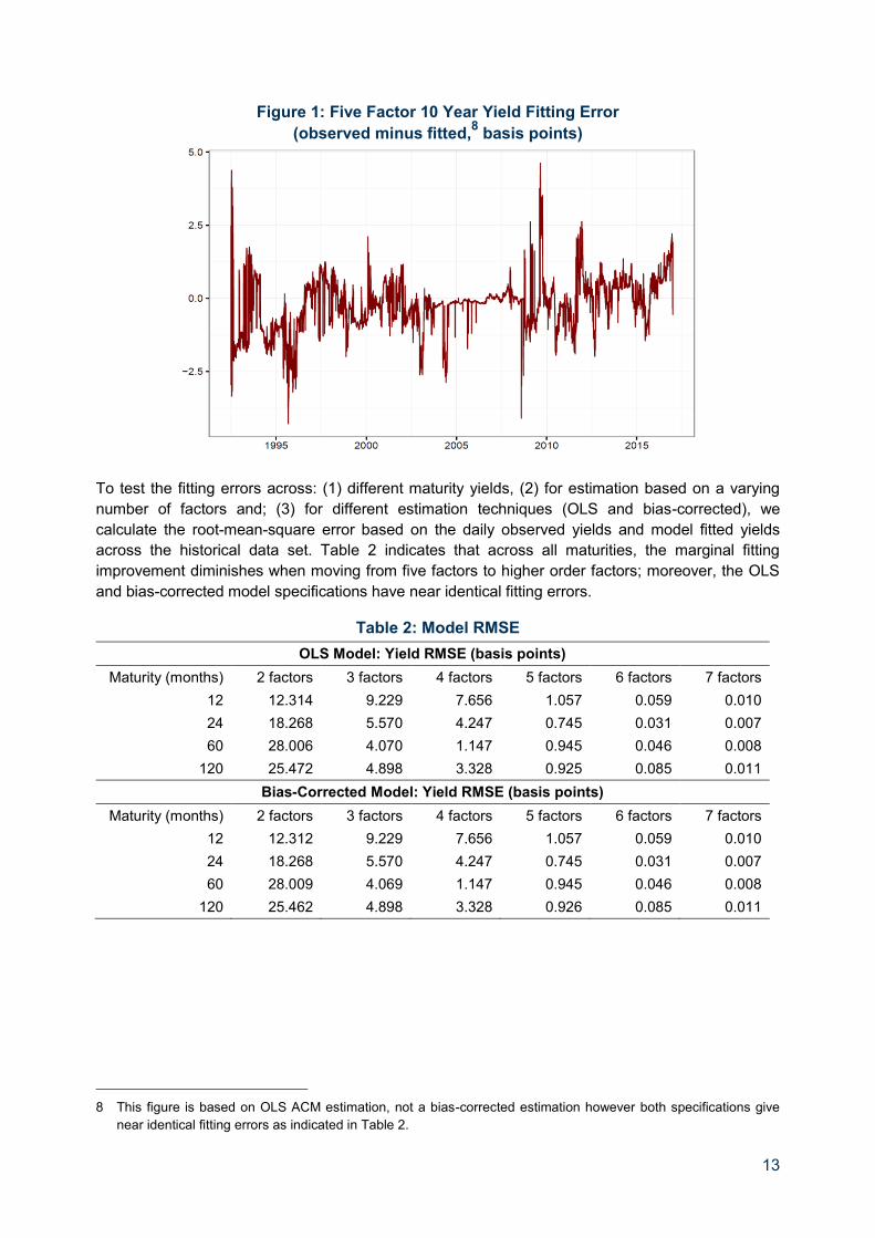
Figure 1: Five Factor 10 Year Yield Fitting Error

(observed minus fitted,8 basis points)

To test the fitting errors across: (1) different maturity yields, (2) for estimation based on a varying

number of factors and; (3) for different estimation techniques (OLS and bias-corrected), we

calculate the root-mean-square error based on the daily observed yields and model fitted yields

across the historical data set. Table 2 indicates that across all maturities, the marginal fitting

improvement diminishes when moving from five factors to higher order factors; moreover, the OLS

and bias-corrected model specifications have near identical fitting errors.

Table 2: Model RMSE

OLS Model: Yield RMSE (basis points)

Maturity (months) 2 factors 3 factors 4 factors 5 factors 6 factors 7 factors

12 12.314 9.229 7.656 1.057 0.059 0.010

24 18.268 5.570 4.247 0.745 0.031 0.007

60 28.006 4.070 1.147 0.945 0.046 0.008

120 25.472 4.898 3.328 0.925 0.085 0.011

Bias-Corrected Model: Yield RMSE (basis points)

Maturity (months) 2 factors 3 factors 4 factors 5 factors 6 factors 7 factors

12 12.312 9.229 7.656 1.057 0.059 0.010

24 18.268 5.570 4.247 0.745 0.031 0.007

60 28.009 4.069 1.147 0.945 0.046 0.008

120 25.462 4.898 3.328 0.926 0.085 0.011

8 This figure is based on OLS ACM estimation, not a bias-corrected estimation however both specifications give

near identical fitting errors as indicated in Table 2.

14

5. MODEL RESULTS

Fitting the five factor ACM model to the Australian Treasury Bond term structure, it is apparent that

a bootstrapped bias-corrected estimation technique gives materially different term premium and

risk-neutral rate estimations relative to the OLS technique. Consistent with BRW, we find that

bias-corrected term structure estimation will result in more variability in risk-neutral rates and

consequently, more stable term premium estimations (Figures 2 and 3).

Figure 2: 10 Year Term Premium Estimates (basis points)

Figure 3: 10 Year Risk Neutral Estimates (percentage points)

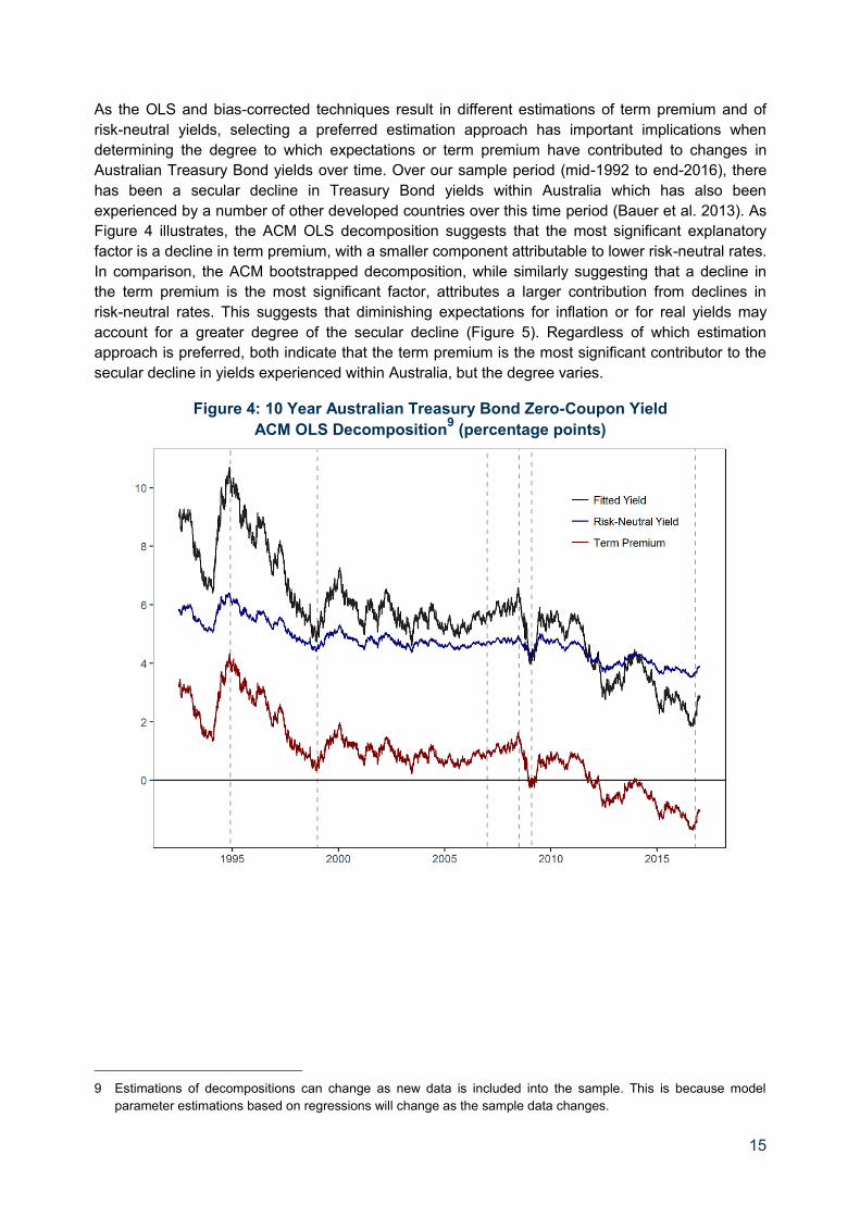
15

As the OLS and bias-corrected techniques result in different estimations of term premium and of

risk-neutral yields, selecting a preferred estimation approach has important implications when

determining the degree to which expectations or term premium have contributed to changes in

Australian Treasury Bond yields over time. Over our sample period (mid-1992 to end-2016), there

has been a secular decline in Treasury Bond yields within Australia which has also been

experienced by a number of other developed countries over this time period (Bauer et al. 2013). As

Figure 4 illustrates, the ACM OLS decomposition suggests that the most significant explanatory

factor is a decline in term premium, with a smaller component attributable to lower risk-neutral rates.

In comparison, the ACM bootstrapped decomposition, while similarly suggesting that a decline in

the term premium is the most significant factor, attributes a larger contribution from declines in

risk-neutral rates. This suggests that diminishing expectations for inflation or for real yields may

account for a greater degree of the secular decline (Figure 5). Regardless of which estimation

approach is preferred, both indicate that the term premium is the most significant contributor to the

secular decline in yields experienced within Australia, but the degree varies.

Figure 4: 10 Year Australian Treasury Bond Zero-Coupon Yield

ACM OLS Decomposition9 (percentage points)

9 Estimations of decompositions can change as new data is included into the sample. This is because model

parameter estimations based on regressions will change as the sample data changes.

16

Figure 5: 10 Year Australian Treasury Bond Zero-Coupon Yield ACM Bootstrapped Bias-Correction Decomposition

(percentage points)

While the OLS and bootstrapped decompositions suggest term premium erosion has been the

primary contributor to the long term declines in yields, these results do not provide insights as to

what has moved the term premium. This is an implication of the ACM term premium estimations

being calculated as a residual, that is, the difference in market yields and risk-neutral yields,

meaning any source of deviation from the pure expectations hypothesis can move the term

premium. This includes typical uncertainty related drivers of the term premium, such as changes in

the degree of macroeconomic uncertainty (uncertainty of future inflation or future real yields) or

changes in the required compensation for that risk (changing levels of risk-aversion such as during

different stages of the business cycle). Other drivers of the term premium captured in the residual

include changes in liquidity or movements based on flight to quality. Flight to quality effects can

cause a significant increase in demand for safe haven assets during times of heightened market

volatility such as during geopolitical risk events (Kim 2007). Flight to quality however is not the only

demand related effect that moves the term premium. In addition to safe haven induced demand, any

significant change in demand for specific securities relative to supply can have an influence through

this channel. For example, the implementation of unconventional monetary policy or ‘quantitative

easing’ via large scale asset purchases by central banks falls into this category. While our model

results do not explicitly decompose the term premium into these various factors, the decompositions

of figures 4 and 5 display some distinct movements of term premium that have coincided with

significant economic events that may allow for inference with respect to what has potentially moved

the term premium at different times over our sample period.

17

For the period from 1995 to 1999, model results (figure 4 and 5) estimate a decline in term premium

and a moderate decline in risk-neutral rates. This period coincided with the implementation of

inflation targeting by the Reserve Bank of Australia. Implicit references to such an objective were

made in 1989 and by mid-1993 it is considered that an inflation targeting objective was more explicit

(Stevens 1999). A declining term premium estimate following on from an explicit inflation targeting

objective is likely to be related to a reduction in the uncertainty of future inflation as central bank

credibility is built over time. Moreover, an accompanying moderate decline in risk-neutral rates

would likely reflect downwards revisions for future inflation as inflation is brought into a target band.

Following on from the late-1990’s, model results suggest term premium remained reasonably stable

up until 2007 which may reflect the Reserve Bank retaining credibility in terms of achieving an

inflation targeting mandate, that is by keeping inflation expectations steady. For the period prior to

the Global Financial Crisis, model estimates suggests the term premium was gradually rising while

risk-neutral rates remained constant. The economic intuition of this is not entirely clear given a

Terms of Trade boom was occurring at the time. Throughout this period, increasing expectations for

inflation, and consequently rising risk-neutral rates would be expected to contribute to yield

movements, not necessarily the term premium.

During the Global Financial Crisis, model results suggest a sharp and sudden decline in term

premium that could be attributed to a flight to quality, reflecting a shift out of risk assets and into

safe haven assets such as Australian Treasury Bonds during a period of heightened risk.

The model results from 2010 to late 2016 suggest a period of further decline in the term premium.

During this time, a number of major central banks undertook unconventional monetary policy

initiatives such as large scale asset purchase programs. This has led to the total assets held by

several major central banks (Federal Reserve, European Central Bank, Bank of Japan) growing

from less than 4 trillion US dollars at the start of 2008 to more than 12 trillion US dollars as at

November 2017 (Yardini Research). Such a large expansion of major central bank balance sheets

presents a significant new source of demand for Government Debt Securities. Through this channel,

the term premium is likely to fall for bonds purchased within these programmes and second order

effects might include term premium (and other risk premia including equity risk premia) falling for

other securities, such as Australian Treasury Bonds.

Model results now show negative term premium estimates that might appear puzzling if viewed from

the prism of a risk averse investor requiring compensation. However, with consideration also given

to other effects influencing the term premium, such as large scale asset purchases, a negative term

premium is entirely plausible. While the term premium remains close to historic lows, a sharp

increase in November 2016 coincided with a broad-based sell off in fixed income assets globally

following the US election.

18

While both estimation approaches lead to broad consensus that a decline in term premium has

been the major factor of a secular decline in Australian Treasury yields, the degree of variation

attributed to risk-neutral rates and term premium estimates differ. As to the question of which

approach is preferred, some research has suggested that bias-corrected parameters may improve

DTSM point estimations (BRW, Diez de los Rios 2014). Other research suggests that applying

bias-correction techniques might lead to less plausible term premium and risk-neutral yield point

estimates compared to OLS estimation (Wright 2014, Malik and Meldrum 2016, Guimaraes 2014).

While there is not necessarily consensus as to whether bias-correction techniques are preferred in

improving DTSM parameter estimation, there is broad consensus that there is uncertainty in the

estimation of DTSM parameters. Given this uncertainty, it is likely that the true data generating

process is likely to be somewhere between the OLS estimated parameters and the bias-corrected

parameters. As such, rather than suggesting an optimal estimation technique, we estimate a daily

Australian Treasury Bond decomposition based on both techniques.

Given the uncertainty of estimation, the best point estimate might actually be a weighted

combination of the OLS and bias-corrected estimation techniques. While in this paper we have not

proposed a method that could be used to find the optimal combination of the OLS and

bias-corrected approaches, development of such an optimisation process could be valuable in

managing the uncertainty of coefficient estimations and thus allow for greater robustness in term

premium and risk-neutral yield estimation. Alternatively, other approaches could be taken such as

anchoring model-estimated expectations to survey data which provides additional information

uncovering how risk-neutral yields evolve.

6. CONCLUSION

We have fitted a linear regression based DTSM to the Australian Treasury Bond term structure and

estimated term premium through a daily yield decomposition. While our estimation approach follows

ACM, we consider an alternative estimation approach that corrects for the potential bias inherent

within a vector autoregressive system when variables are highly persistent. Our findings show that

this alternative specification leads to significantly different term premium estimations and more

variability in risk-neutral yields. Given this variation in estimation, we provide and analyse yield

decompositions with and without this alternative estimation approach and suggest that the true data

generating process most likely lies somewhere within the bounds of these model specifications.

However, regardless of which estimation approach is preferred, both indicate that the term premium

is the most significant contributor to the secular decline in yields experienced within Australia, but

the degree varies. In this paper, no attempt is made to suggest an optimal estimation approach.

However, finding a preferred combination of these alternative estimation techniques could be

valuable in managing the uncertainty of coefficient estimations and ultimately allow for greater

robustness in term premium estimation.

19

REFERENCES

Adrian, T., Crump, R.K. and Moench, E., 2013. Pricing the term structure with linear regressions.

Journal of Financial Economics, 110(1), pp.110-138.

Bauer, M.D., Rudebusch, G.D. and Wu, J.C., 2012. Correcting estimation bias in dynamic term

structure models. Journal of Business & Economic Statistics, 30(3), pp.454-467.

Bauer, M.D., Rudebusch, G.D. and Wu, J.C., 2014. Term premia and inflation uncertainty: Empirical

evidence from an international panel dataset: Comment. The American Economic Review, 104(1),

pp.323-337

Campbell, J.Y. and Shiller, R.J., 1991. Yield spreads and interest rate movements: A bird's eye

view. The Review of Economic Studies, 58(3), pp.495-514.

Cox, J.C., Ingersoll Jr, J.E. and Ross, S.A., 1985. A theory of the term structure of interest

rates. Econometrica: Journal of the Econometric Society, pp.385-407.

Dai, Q. and Singleton, K.J., 2002. Expectation puzzles, time-varying risk premia, and affine models

of the term structure. Journal of financial Economics, 63(3), pp.415-441.

Duffie, D. and Kan, R., 1996. A yield‐factor model of interest rates. Mathematical finance, 6(4),

pp.379-406.

Duffee, G.R., 2002. Term premia and interest rate forecasts in affine models. The Journal of

Finance, 57(1), pp.405-443.

Fama, E.F. and MacBeth, J.D., 1973. Risk, return, and equilibrium: Empirical tests. The journal of

political economy, pp.607-636.

Finlay, R. and Olivan, D., 2012. Extracting Information from Financial Market Instruments. The RBA

Bulletin March Quarter, pp.45

Finlay, Richard, and Mark Chambers. "A term structure decomposition of the Australian yield curve."

Economic Record 85.271 (2009): 383-400.

Finlay, Richard, and Sebastian Wende. "Estimating Inflation Expectations with a Limited Number of

Inflation-Indexed Bonds." International Journal of Central Banking (2012).

Hamilton, J. and Wu, J., 2010. Identification and estimation of affine term structure models. Working

paper, University of California, San Diego.

Kim, D.H. and Orphanides, A., 2005. Term structure estimation with survey data on interest rate

forecasts.

Kim, D.H. and Orphanides, A., 2007. The bond market term premium: what is it, and how can we

measure it?. BIS Quarterly Review, June.

Kim, D.H. and Wright, J.H., 2005. An arbitrage-free three-factor term structure model and the recent

behavior of long-term yields and distant-horizon forward rates.

20

Kilian, L., 1998. Small-sample confidence intervals for impulse response functions. Review of

economics and statistics, 80(2), pp.218-230.

Krippner, L. and Callaghan, M., 2016. Short-term risk premiums and policy rate expectations in the

United States. Reserve Bank of New Zealand Analytical Note Series

Malik, S. and Meldrum, A., 2014. Evaluating the robustness of UK term structure decompositions

using linear regression methods. Bank of England Working paper No.518

Malik, S. and Meldrum, A., 2016. Evaluating the robustness of UK term structure decompositions

using linear regression methods. Journal of Banking & Finance, 67, pp.85-102.

Nelson, C.R. and Siegel, A.F., 1987. Parsimonious modeling of yield curves. Journal of business,

pp.473-489.

Pope, A.L., 1990. Biases of estimators in multivariate non-Gaussian autoregression. Journal of

Time Series Analysis, 11(3), pp.249-258.

Glenn, S. (1999). Six Years of Inflation Targeting. (Economic Society of Australia, Speech)

Guimarães, R., 2014. Expectations, risk premia and information spanning in dynamic term structure

model estimation. Bank of England Working paper No.489

Svensson, L.E., 1994. Estimating and interpreting forward interest rates: Sweden 1992-1994

(No. w4871). National bureau of economic research.

Vasicek, O., 1977. An equilibrium characterization of the term structure. Journal of financial

economics, 5(2), pp.177-188

Wright, J.H., 2011. Term premia and inflation uncertainty: Empirical evidence from an international

panel dataset. The American Economic Review, 101(4), pp.1514-1534.

Wright, J.H., 2014. Term Premia and Inflation Uncertainty: Empirical Evidence from an International

Panel Dataset: Reply. The American Economic Review, 104(1), pp.338-341.

Yardeni, E. (2017). Global Economic Briefing: Central Bank Balance Sheets. 1st ed. [ebook]

Yardeni Research, Inc., p.1. Available at: http://www.yardeni.com/pub/peacockfedecbassets.pdf

[Accessed 6 Jan. 2017].