Estimation of tropical forest height and biomass dynamics ...biology/files/pdfs/dave-clark/Dubayah...

ClickHere

for

FullArticle

Estimation of tropical forest height and biomass dynamicsusing lidar remote sensing at La Selva, Costa Rica

R. O. Dubayah,1 S. L. Sheldon,1 D. B. Clark,2,3 M. A. Hofton,1 J. B. Blair,4 G. C. Hurtt,5

and R. L. Chazdon6

Received 13 January 2009; revised 24 September 2009; accepted 2 November 2009; published 9 April 2010.

[1] In this paper we present the results of an experiment to measure forest structure andbiomass dynamics over the tropical forests of La Selva Biological Station in Costa Ricausing a medium resolution lidar. Our main objective was to observe changes in forestcanopy height, related height metrics, and biomass, and from these map sources and sinksof carbon across the landscape. The Laser Vegetation Imaging Sensor (LVIS) measuredcanopy structure over La Selva in 1998 and again in 2005. Changes in waveformmetrics were related to field‐derived changes in estimated aboveground biomass from aseries of old growth and secondary forest plots. Pairwise comparisons of nearly coincidentlidar footprints between years showed canopy top height changes that coincided withexpected changes based on land cover types. Old growth forests had a net loss in height of−0.33 m, while secondary forests had net gain of 2.08 m. Multiple linear regressionwas used to relate lidar metrics with biomass changes for combined old growth andsecondary forest plots, giving an r2 of 0.65 and an RSE of 10.5 Mg/ha, but both parametricand bootstrapped confidence intervals were wide, suggesting weaker model performance.The plot level relationships were then used to map biomass changes across La Selvausing LVIS at a 1 ha scale. The spatial patterns of biomass changes matched expectedpatterns given the distribution of land cover types at La Selva, with secondary forestsshowing a gain of 25 Mg/ha and old growth forests showing little change (2 Mg/ha).Prediction intervals were calculated to assess uncertainty for each 1 ha cell to ascertainwhether the data and methods used could confidently estimate the sign (source or sink)of the biomass changes. The resulting map showed most of the old growth areas as neutral(no net biomass change), with widely scattered and isolated sources and sinks. Secondaryforests in contrast were mostly sinks or neutral, but were never sources. By quantifyingboth the magnitude of biomass changes and the sensitivity of lidar to detect them, thiswork will help inform the formulation of future space missions focused on biomassdynamics, such as NASA’s Deformation Ecosystem Structure and Dynamics of Ice mission.

Citation: Dubayah, R. O., S. L. Sheldon, D. B. Clark, M. A. Hofton, J. B. Blair, G. C. Hurtt, and R. L. Chazdon (2010),Estimation of tropical forest height and biomass dynamics using lidar remote sensing at La Selva, Costa Rica, J. Geophys. Res.,115, G00E09, doi:10.1029/2009JG000933.

1. Introduction

[2] Forests are the focus of intense research in globalenvironmental change. The effects on carbon of natural and

anthropogenic forest structural changes and dynamics are ofparticular interest. A major source of error in estimates ofland surface carbon and other biogeochemical fluxes arisesfrom uncertainty in prescribing initial forest carbon stocks,and subsequent changes to these from growth, degradationand deforestation [Brown, 1997;Houghton et al., 2001;Clark,2004; Houghton and Goetz, 2008]. Furthermore, attemptsto understand and predict how tropical forests will respondto continued global changes in climate will require refinedand spatially explicit estimates of biomass and other foreststructure changes [Clark, 2004].[3] New remote sensing technologies have the potential to

provide these estimates by quantifying stocks, sources, andsinks of land surface carbon [Houghton and Goetz, 2008].Among these technologies is lidar remote sensing. Studiesusing airborne and spaceborne lidar have validated its ability

1Department of Geography, University of Maryland, College Park,Maryland, USA.

2Department of Biology, University of Missouri at St. Louis, SaintLouis, Missouri, USA.

3La Selva Biological Station, La Selva, Costa Rica.4Laser Remote Sensing Laboratory, NASA Goddard Space Flight

Center, Greenbelt, Maryland, USA.5Institute for the Study of Earth, Oceans, and Space, University of New

Hampshire, Durham, New Hampshire, USA.6Ecology and Evolutionary Biology, University of Connecticut, Storrs,

Connecticut, USA.

Copyright 2010 by the American Geophysical Union.0148‐0227/10/2009JG000933

JOURNAL OF GEOPHYSICAL RESEARCH, VOL. 115, G00E09, doi:10.1029/2009JG000933, 2010

G00E09 1 of 17

http://dx.doi.org/10.1029/2009JG000933

to retrieve many aspects of forest structure important forcarbon and ecosystem studies, including canopy height, leafdistribution, and aboveground biomass stocks [Lefsky et al.,2002; Drake et al., 2002a; Clark et al., 2004; Naesset andGobakken, 2005]. Three NASA missions have used lidaras a central aspect of an observing strategy for forest struc-ture. The first was the Vegetation Canopy Lidar (VCL)which was never launched [Dubayah et al., 1997]. The sec-ond is the ICESAT (Ice, Cloud, and land Elevation Satellite)mission [Lefsky et al., 2005] currently in orbit. The third is theplanned DESDynI (Deformation, Ecosystem Structure, andDynamics of Ice) mission [Donnellan et al., 2008]. DESDynIwill combine a multibeam lidar with polarimetric and inter-ferometric SAR capability to measure forest structure, bio-mass, and their dynamics. One of the motivations of ourresearch is to explore the efficacy of lidar for capturing foreststructural changes to help inform planning of the DESDynImission.[4] A major application of forest structure data from

DESDynI and other sources is for carbon flux modeling.Forests are typically a heterogeneous mixture of stands ofdifferent successional age and both ecosystem structure andcarbon fluxes vary strongly with successional status. Thisheterogeneity is typically manifested through variability incanopy height. Observations of these heights by lidar providelarge clues to the successional state of the vegetation. Theassumption is that taller trees are older and shorter trees areyounger. Using lidar‐derived heights under this assumptionin ecosystem modeling greatly constrains model estimates ofaboveground biomass and associated carbon flux betweenthe vegetation and the atmosphere [Hurtt et al., 2004; Thomaset al., 2008].[5] However, knowledge of canopy height alone is not

always sufficient to ascertain successional status and there-fore the sign (source or sink) and magnitude of carbon fluxesfor particular areas, even when initial carbon stocks are cor-rectly determined. This is because stands may be short notbecause they are young, but rather because they are limitedby edaphic and climatic conditions [Clark and Clark, 2000].Modeled fluxes will then vary greatly depending on theprescribed successional state. One way to overcome theseobstacles is to directly measure canopy changes by acquiringtwo or more sets of canopy structure observations separatedin time [Kellner et al., 2009]. Successional status may beinferred, rates of regrowth and mortality directly observed,and biomass accumulation and loss more directly modeled.Given the difficulties of measuring canopy dynamics in thefield, there is considerable uncertainty about rates of regrowthand mortality in tropical forests. Furthermore, the efficacy ofwaveform lidar, such as used from spaceborne missions, todetermine such changes across a tropical land use gradienthas not been demonstrated.[6] In this paper we present the results of an experiment to

measure canopy structure dynamics over the tropical forestsof La Selva Biological Station in Costa Rica between theyears 1998 and 2005 using a medium resolution (25 mfootprint) lidar. Our main objective was to observe changes inforest canopy height, related height metrics, and estimatedaboveground biomass (hereafter “biomass”), and from thesemap sources and sinks of carbon across the landscape. Thisresearch further provides an assessment of the capability ofmedium resolution, waveform lidar to determine canopy

changes over subdecadal time spans. By quantifying both themagnitude of the changes, as well as the sensitivity of lidar todetect them, this work will help inform the formulation offuture space missions focused on biomass dynamics, such asDESDynI.

2. Lidar Remote Sensing at La Selva

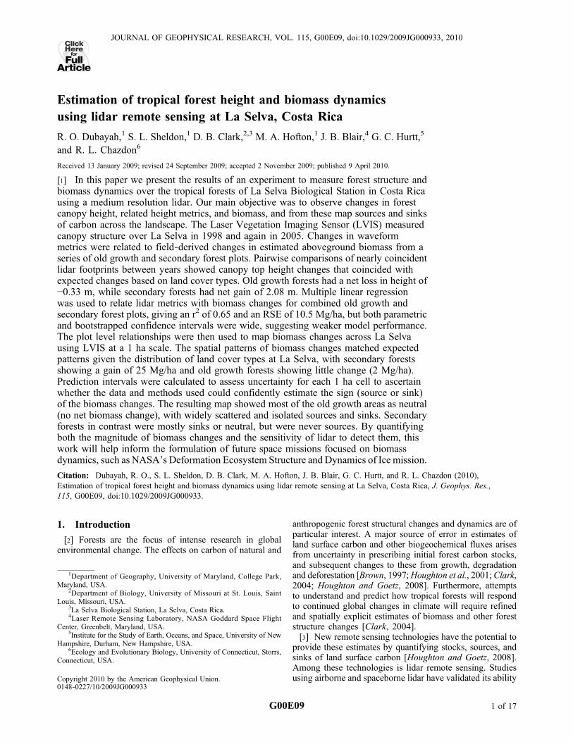
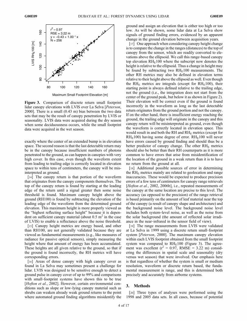
[7] La Selva Biological Station is located in northeastCosta Rica. The area is renowned for the depth, variety, andhistory of its biological data sets, and is among the moststudied field sites in the humid tropics. The topography ofthe area is varied but low lying (<150 m) and receives 4 mof rain on average per year (see McDade et al. [1994] forfull overview of La Selva). The Station proper is a mix ofold growth and secondary lowland Tropical Wet Forest[Hartshorn and Hammel, 1994], along with remnant plan-tations and various agroforestry treatments. As part of a long‐term study called the Carbono Project [Clark and Clark,2000], all stems ≥10 cm diameter (at 1.3 m height or abovebasal irregularities like buttresses) in a network of 180.5 haold growth plots are censused annually for growth, mortalityand recruitment. Plot‐level basal area and allometricallyestimated aboveground biomass (EAGB) are calculatedyearly [Clark and Clark, 2000]. We used EAGB data fromthe September–October 1997 and September–October 2004Carbono censuses to comparewith lidar data acquired in 1998and 2005. Additionally, information including stand age,basal area, EAGB, and tree density were collected for allstems >5 cm diameter in two, 1 ha secondary forest plotsat La Selva during the study period [Chazdon et al., 2007].Stem diameter is used to calculate EAGB using Brown’s[1997] equation for tropical wet forests. These field dataare summarized in Table 1 and Figure 1.[8] Lidar data were acquired over the La Selva region by

the Laser Vegetation Imaging Sensor (LVIS) [Blair et al.,1999]. LVIS is a medium altitude, waveform digitizing lidar.Footprint size can be varied, but it is usually flown in amediumresolution format with diameters from 10 to 30 m. The returnsignal is digitized to correspond to a vertical resolution of30 cm that provides a vertical record of intercepted canopysurfaces. From each waveform, canopy height, canopy ver-tical metrics, and subcanopy topography may be directlyderived, relative to the WGS‐84 ellipsoid (see Hofton andBlair [2002] and Hofton et al. [2002, 2006a] for moredetails). Waveforms are geolocated generally to within 2 mor better [Blair and Hofton, 1999].[9] LVIS was flown over La Selva in March 1998 at an

altitude of 8 km. Nominal footprint diameters were 25 m,with 80 footprints scanned across track (separated by 25 m),and 9 m separation (overlapping) along track [Hofton et al.,2002]. La Selva was then reflown by LVIS in March 2005 atan altitude of 10 km. The swath width in 2005 was 2 km,using 25 m footprints with 20 m spacing along track andacross track. The initial 1998 flight was a part of a cali-bration and validation campaign for the VCL mission.[10] Although LVIS is an imaging lidar, the images are

made up individual footprints. For various reasons, such ascloud cover, flight path irregularities, pointing and noise,among others, portions of the landscape may not be com-pletely mapped. In addition, because footprints overlap andthere are often overlapping flight lines, some portions may

DUBAYAH ET AL.: FOREST DYNAMICS USING LIDAR G00E09G00E09

2 of 17

be mapped several times during the same campaign. Thus agiven area on the ground may have varying numbers ofspatially irregular lidar observations (given in Table 1) eitherbetween plots or between years.[11] Although canopy height is a primary measurement,

other waveform metrics are calculated. Among these are therelative height (RH) metrics associated with energy quan-tiles (25%, 50%, and 75%). For example, the RH50 metricor HOME (height of median energy) is the height above the

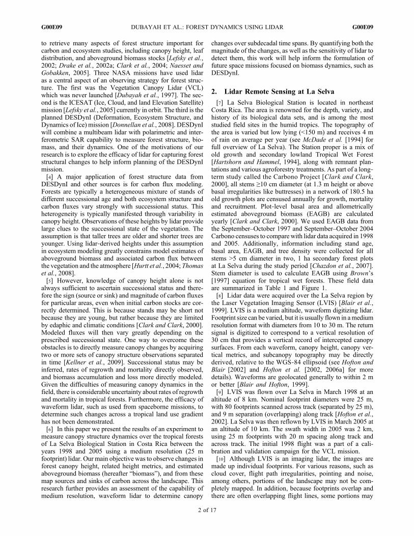
ground elevation at which 50% of the returned energy in thewaveform (including the ground portion of the return) isabove and 50% below. We calculate these metrics becausethey have been shown to be useful predictors of biomass andof canopy vertical structure [Drake et al., 2002a, 2002b,2003; Duong et al., 2008].[12] Some of the essential features of the waveform are

shown in Figure 2. The entire “extent” of the waveform isfirst positioned in absolute elevation space relative to anellipsoid (such as WGS‐84). The extent goes from the firstreturn above a noise threshold (the “leading edge”) to thelast return above the noise threshold (the “trailing edge”).The ground return is that portion of the waveform that ori-ginates from reflectance off the ground underneath thecanopy and is found by starting at the trailing edge andsubsequently finding an inflection point or peak where theslope of the waveform changes from positive to negative.The strength of this return is dependent on several factors,but most importantly on canopy cover, ground reflectanceand slope. The elevation of the ground return is specified asthe center of the ground return portion. The location of theground, in elevation space, must always be above thetrailing edge.[13] The ground return ordinarily is strong and there is

usually little doubt about its elevation. However, for weakreturns there is often an element of interpretation. Thisoccurs for two reasons. The first is that weak returns seldomshow sharp central peaks, so that automated algorithms eitherinterpret other peaks as ground or have difficulty deciding

Table 1. Estimated Aboveground Biomass Data From La Selvaa

ID

Biomass (Mg/ha)Biomass

Change (Mg/ha),2005–1998

Number of LidarObservations

1998 2005 1998 2005

a1 176.11 181.06 4.95 35 65a2 135.32 150.26 14.94 35 16a3 166.87 157.59 −9.28 23 34a4 178.20 186.26 8.06 25 33a5 180.79 197.81 17.02 26 27a6 161.71 177.27 15.56 11 51l1 134.66 120.91 −13.75 20 38l2 135.84 119.63 −16.22 25 32l3 180.37 163.70 −16.67 13 46l4 133.45 118.99 −14.46 20 50l5 157.96 151.61 −6.35 17 63l6 160.34 169.28 8.94 21 63lep* 144.67 175.62 30.95 62 40lsur* 90.73 142.08 51.34 20 38p1 105.53 123.52 17.99 26 26p2 137.94 137.71 −0.22 17 20p3 162.15 163.43 1.28 23 49p4 172.23 182.12 9.89 9 45p5 194.95 192.94 −2.00 29 54p6 160.61 143.47 −17.14 19 40

aLidar observations refer to the number of lidar footprints that fell withina plot in a particular year. Plots labeled “a” are on flat inceptisols, “l” plotsare on flat ultisols, and “p” plots are on steep ultisol slopes. Plots lep* andlsur* are 1.0 ha secondary forest plots. All others are 0.5 ha old growthplots of the Carbono project.

Figure 1. Changes in EAGB for 18 old growth Carbonoplots and two secondary forest plots. Over the 7 year period,changes in EAGB for the Carbono plots were mostly bal-anced between those that gained and those that lost biomass(sinks and sources, respectively), whereas the two secondaryplots were strong sinks.

Figure 2. Components of a return lidar waveform. Theendpoints of the waveform extent are positioned in elevationspace relative to the WGS‐84 ellipsoid. The RH metrics arethe quantiles of the cumulative return (the monotonicallyincreasing curve) starting at the trailing edge, but expressedas a height above the interpreted ground return. RH100 corre-sponds to height above the ground of the highest reflectingsurface that triggers a return above the noise level. Becauseof canopy penetration, this height may be below the actualtallest leaves in the canopy. The ground portion of the returnis shown as bold.


3 of 17

exactly where the center of an extended bump is in elevationspace. The second reason is that the last detectable return maybe in the canopy because insufficient numbers of photonspenetrated to the ground, as can happen in canopies with veryhigh cover. In this case, even though the waveform extentfrom leading to trailing edge is correctly located in elevationspace to within tens of centimeters, the canopy will be mis-interpreted as ground.[14] The canopy return is that portion of the waveform

that originates from the canopy components themselves. Thetop of the canopy return is found by starting at the leadingedge of the return until a signal greater then some noisethreshold is found. Maximum canopy height above theground (RH100) is found by subtracting the elevation of theleading edge of the waveform from the determined groundelevation. This maximum height is more properly viewed asthe “highest reflecting surface height” because it is depen-dent on sufficient canopy material (about 0.5 m2 in the caseof LVIS) to enable a reflectance above the noise threshold.[15] Canopy height metrics are energy based, and other

than RH100, are not generally validated because they areviewed as fundamental measurements (e.g., like measures ofradiance for passive optical sensors), simply measuring theheight where that amount of energy has been accumulated.These heights are all given relative to the ground, so that ifthe ground is found incorrectly, the RH metrics will havecorresponding errors.[16] Areas of dense canopy with high canopy cover as

found in La Selva may sometimes present a challenge forlidar. LVIS was designed to be sensitive enough to detect aground pulse in canopy cover of up to 99% and comparisonswith small‐footprint systems have shown this to be true[Hofton et al., 2002]. However, certain environmental con-ditions such as slope or low‐lying canopy material such asshrubs can weaken already weak ground returns to the pointwhere automated ground finding algorithms misidentify the

ground and assign an elevation that is either too high or toolow. As will be shown, some lidar data at La Selva showsignals of ground finding errors, evidenced by an apparentchange in the ground elevation between acquisition years.[17] One approach when considering canopy height change

is to compare the change in the ranges (distances) to the top ofcanopy from the sensor, which are readily converted to ele-vations above the ellipsoid. We call this range‐based canopytop elevation RHE100 where the subscript now denotes theheight is relative to the ellipsoid. Thus a change in height maybe found by subtracting two RHE100 measurements. Theother RH metrics may also be defined in elevation termsrelative to their height above the ellipsoid as well. Even thoughthe RHE metrics are integrals (except for RHE100), theirstarting point is always defined relative to the trailing edge,not the ground (i.e., the integration does not start from thecenter of the ground peak, but below it as shown in Figure 2).Their elevation will be correct even if the ground is foundincorrectly in the waveform as long as the last detectablereturn originates from the ground portion and not the canopy.If on the other hand, there is insufficient energy reaching theground, the trailing edge will originate in the canopy and thiscanopy return will be misinterpreted as ground, even thoughthe waveform is correctly located in elevation space. Thiswould result in and both the RH and RHE metrics (except forRHE100) having some degree of error. RHE100 will neverhave errors caused by ground finding and should thus be abetter predictor of canopy change. The other RHE metricsshould also be better than their RH counterparts as it is morecommon to have errors that arise from misidentification ofthe location of the ground in a weak return than it is to haveno return from the ground at all.[18] Additional possible sources of error in determining

the RHE metrics mainly are related to geolocation and rangeinaccuracies. These would be expected to produce precisionerrors of a few tens of centimeters for canopy range retrievals[Hofton et al., 2002, 2006b], i.e., repeated measurements ofthe canopy at the same location are precise to this level. Theaccuracy (as opposed to the precision) of the range retrievalis based primarily on the amount of leaf material near the topof the canopy (a result of canopy shape and architecture) andthe background noise level. The background noise levelincludes both system‐level noise, as well as the noise fromthe solar background (the amount of reflected solar irradi-ance in the near‐infrared in the sensor field of view).[19] The range measurements from LVIS were validated

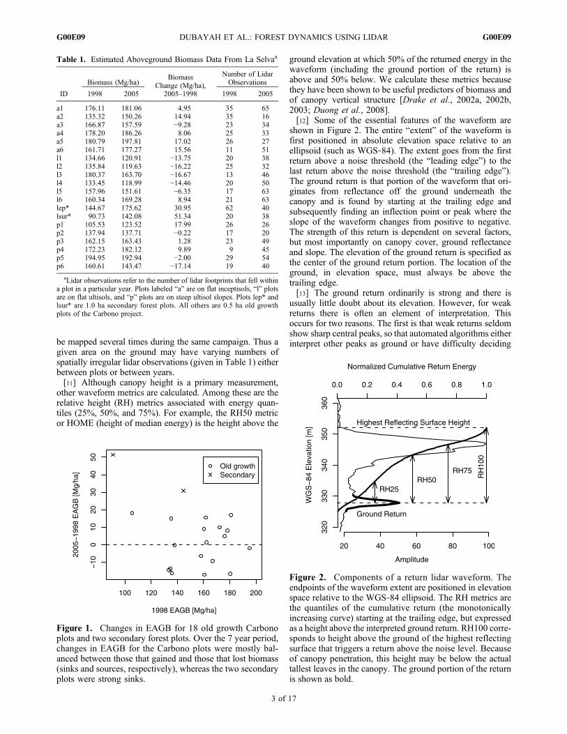
at La Selva in 1999 using a discrete return small‐footprintsystem [Peterson, 2000]. The maximum canopy elevationwithin each LVIS footprint obtained from the small footprintsystem was compared to RHE100 (Figure 3). The agree-ment was excellent (r2 = 0.97, RMSE = 3.22 m) consid-ering the differences in spatial scale and seasonality (dryversus wet season) that were involved. Our emphasis hereis that regardless of whether the system is small or mediumresolution, waveform or discrete return based, the funda-mental measurement is range, and this is determined bothprecisely and accurately from airborne systems.

3. Methods

[20] Three types of analyses were performed using the1998 and 2005 data sets. In all cases, because of potential

Figure 3. Comparison of discrete return small footprintlidar canopy elevations with LVIS over La Selva [Peterson,2000]. There is a small (0.43 m) bias between the two datasets that may be the result of canopy penetration by LVIS orseasonality. LVIS data were acquired during the dry seasonwhen some deciduousness occurs, while the small footprintdata were acquired in the wet season.


4 of 17

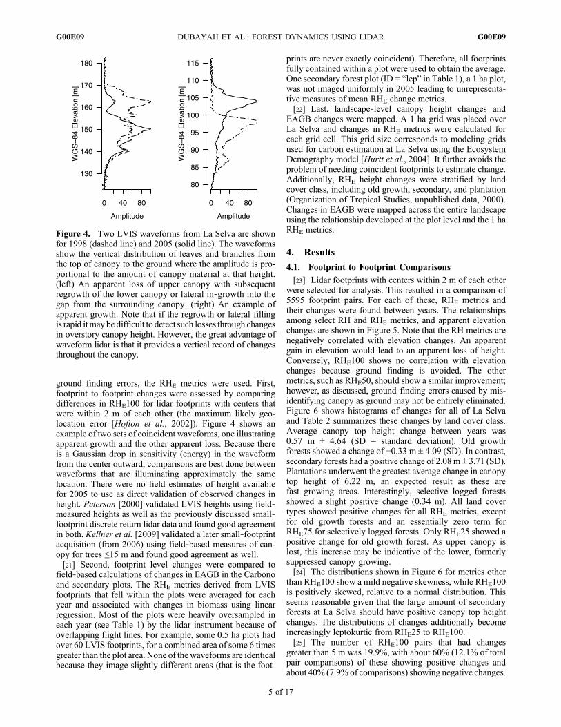
ground finding errors, the RHE metrics were used. First,footprint‐to‐footprint changes were assessed by comparingdifferences in RHE100 for lidar footprints with centers thatwere within 2 m of each other (the maximum likely geo-location error [Hofton et al., 2002]). Figure 4 shows anexample of two sets of coincident waveforms, one illustratingapparent growth and the other apparent loss. Because thereis a Gaussian drop in sensitivity (energy) in the waveformfrom the center outward, comparisons are best done betweenwaveforms that are illuminating approximately the samelocation. There were no field estimates of height availablefor 2005 to use as direct validation of observed changes inheight. Peterson [2000] validated LVIS heights using field‐measured heights as well as the previously discussed small‐footprint discrete return lidar data and found good agreementin both. Kellner et al. [2009] validated a later small‐footprintacquisition (from 2006) using field‐based measures of can-opy for trees ≤15 m and found good agreement as well.[21] Second, footprint level changes were compared to

field‐based calculations of changes in EAGB in the Carbonoand secondary plots. The RHE metrics derived from LVISfootprints that fell within the plots were averaged for eachyear and associated with changes in biomass using linearregression. Most of the plots were heavily oversampled ineach year (see Table 1) by the lidar instrument because ofoverlapping flight lines. For example, some 0.5 ha plots hadover 60 LVIS footprints, for a combined area of some 6 timesgreater than the plot area. None of the waveforms are identicalbecause they image slightly different areas (that is the foot-

prints are never exactly coincident). Therefore, all footprintsfully contained within a plot were used to obtain the average.One secondary forest plot (ID = “lep” in Table 1), a 1 ha plot,was not imaged uniformly in 2005 leading to unrepresenta-tive measures of mean RHE change metrics.[22] Last, landscape‐level canopy height changes and

EAGB changes were mapped. A 1 ha grid was placed overLa Selva and changes in RHE metrics were calculated foreach grid cell. This grid size corresponds to modeling gridsused for carbon estimation at La Selva using the EcosystemDemography model [Hurtt et al., 2004]. It further avoids theproblem of needing coincident footprints to estimate change.Additionally, RHE height changes were stratified by landcover class, including old growth, secondary, and plantation(Organization of Tropical Studies, unpublished data, 2000).Changes in EAGB were mapped across the entire landscapeusing the relationship developed at the plot level and the 1 haRHE metrics.

4. Results

4.1. Footprint to Footprint Comparisons

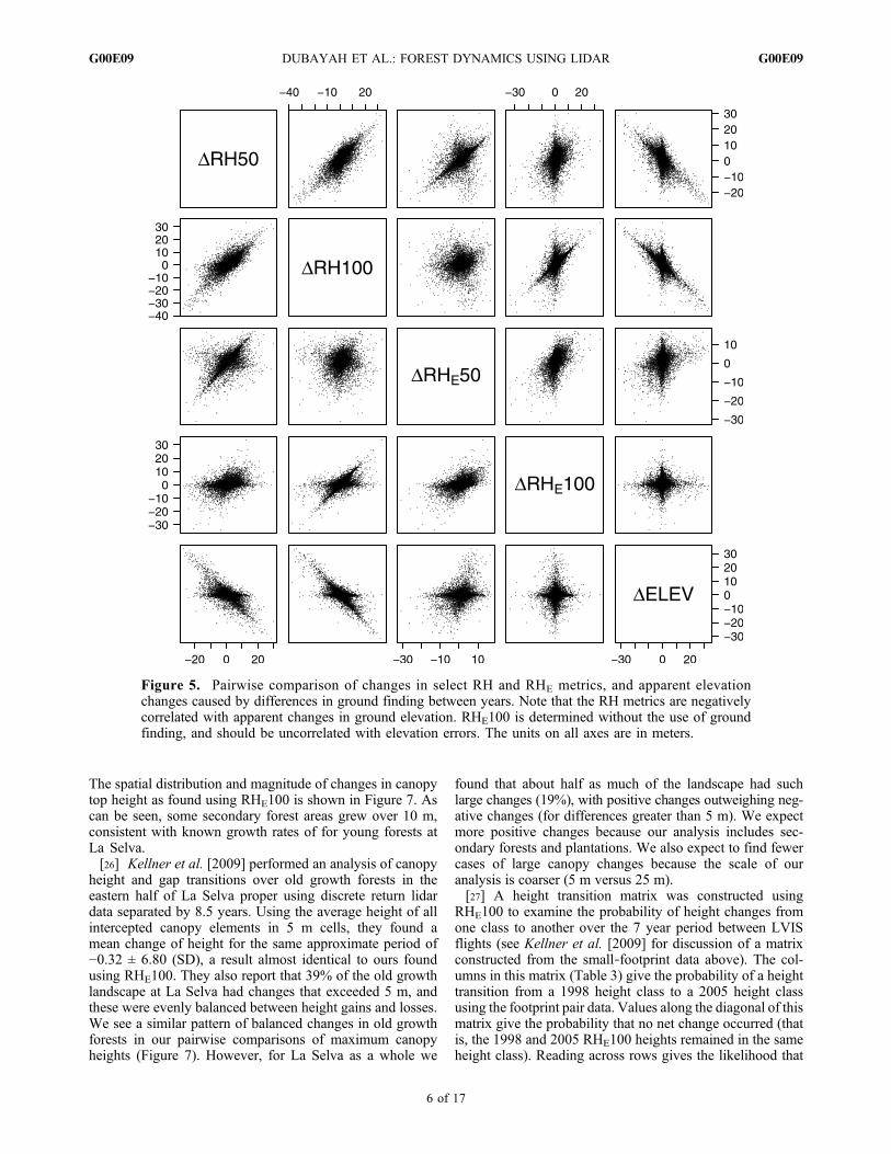
[23] Lidar footprints with centers within 2 m of each otherwere selected for analysis. This resulted in a comparison of5595 footprint pairs. For each of these, RHE metrics andtheir changes were found between years. The relationshipsamong select RH and RHE metrics, and apparent elevationchanges are shown in Figure 5. Note that the RH metrics arenegatively correlated with elevation changes. An apparentgain in elevation would lead to an apparent loss of height.Conversely, RHE100 shows no correlation with elevationchanges because ground finding is avoided. The othermetrics, such as RHE50, should show a similar improvement;however, as discussed, ground‐finding errors caused by mis-identifying canopy as ground may not be entirely eliminated.Figure 6 shows histograms of changes for all of La Selvaand Table 2 summarizes these changes by land cover class.Average canopy top height change between years was0.57 m ± 4.64 (SD = standard deviation). Old growthforests showed a change of −0.33 m ± 4.09 (SD). In contrast,secondary forests had a positive change of 2.08m ± 3.71 (SD).Plantations underwent the greatest average change in canopytop height of 6.22 m, an expected result as these arefast growing areas. Interestingly, selective logged forestsshowed a slight positive change (0.34 m). All land covertypes showed positive changes for all RHE metrics, exceptfor old growth forests and an essentially zero term forRHE75 for selectively logged forests. Only RHE25 showed apositive change for old growth forest. As upper canopy islost, this increase may be indicative of the lower, formerlysuppressed canopy growing.[24] The distributions shown in Figure 6 for metrics other

than RHE100 show a mild negative skewness, while RHE100is positively skewed, relative to a normal distribution. Thisseems reasonable given that the large amount of secondaryforests at La Selva should have positive canopy top heightchanges. The distributions of changes additionally becomeincreasingly leptokurtic from RHE25 to RHE100.[25] The number of RHE100 pairs that had changes

greater than 5 m was 19.9%, with about 60% (12.1% of totalpair comparisons) of these showing positive changes andabout 40% (7.9% of comparisons) showing negative changes.

Figure 4. Two LVIS waveforms from La Selva are shownfor 1998 (dashed line) and 2005 (solid line). The waveformsshow the vertical distribution of leaves and branches fromthe top of canopy to the ground where the amplitude is pro-portional to the amount of canopy material at that height.(left) An apparent loss of upper canopy with subsequentregrowth of the lower canopy or lateral in‐growth into thegap from the surrounding canopy. (right) An example ofapparent growth. Note that if the regrowth or lateral fillingis rapid itmay be difficult to detect such losses through changesin overstory canopy height. However, the great advantage ofwaveform lidar is that it provides a vertical record of changesthroughout the canopy.


5 of 17

The spatial distribution and magnitude of changes in canopytop height as found using RHE100 is shown in Figure 7. Ascan be seen, some secondary forest areas grew over 10 m,consistent with known growth rates of for young forests atLa Selva.[26] Kellner et al. [2009] performed an analysis of canopy

height and gap transitions over old growth forests in theeastern half of La Selva proper using discrete return lidardata separated by 8.5 years. Using the average height of allintercepted canopy elements in 5 m cells, they found amean change of height for the same approximate period of−0.32 ± 6.80 (SD), a result almost identical to ours foundusing RHE100. They also report that 39% of the old growthlandscape at La Selva had changes that exceeded 5 m, andthese were evenly balanced between height gains and losses.We see a similar pattern of balanced changes in old growthforests in our pairwise comparisons of maximum canopyheights (Figure 7). However, for La Selva as a whole we

found that about half as much of the landscape had suchlarge changes (19%), with positive changes outweighing neg-ative changes (for differences greater than 5 m). We expectmore positive changes because our analysis includes sec-ondary forests and plantations. We also expect to find fewercases of large canopy changes because the scale of ouranalysis is coarser (5 m versus 25 m).[27] A height transition matrix was constructed using

RHE100 to examine the probability of height changes fromone class to another over the 7 year period between LVISflights (see Kellner et al. [2009] for discussion of a matrixconstructed from the small‐footprint data above). The col-umns in this matrix (Table 3) give the probability of a heighttransition from a 1998 height class to a 2005 height classusing the footprint pair data. Values along the diagonal of thismatrix give the probability that no net change occurred (thatis, the 1998 and 2005 RHE100 heights remained in the sameheight class). Reading across rows gives the likelihood that

Figure 5. Pairwise comparison of changes in select RH and RHE metrics, and apparent elevationchanges caused by differences in ground finding between years. Note that the RH metrics are negativelycorrelated with apparent changes in ground elevation. RHE100 is determined without the use of groundfinding, and should be uncorrelated with elevation errors. The units on all axes are in meters.


6 of 17

an observed height in 2005 originated from the height class inthat column from 1998. In general, the diagonal shows anincreasing trend: the larger the canopy height in 1998, themore likely it was to remain in that class. For shorter canopyheights (<30 m) transition probabilities are strongly weightedtoward positive height gains. For the shortest canopies in1998, observed canopy top height changes could be 20 m ormore reflecting the large growth changes young secondaryforests can exhibit. For 1998 heights in presumably olderforests in the 30–40 m class, transition probabilities are rel-atively equally weighted between changes to higher and lowerheight classes. These areas appear to be in a type of balance onthe whole, where transitions to higher height classes throughgrowth are about as likely as transitions to lower height classesthrough disturbance and mortality. As we reach the limits ofcanopy height at La Selva, transitions must necessarily bemore likely into lower height classes.[28] Our data suggest that footprints from the shortest

height class can transition to a much higher class (see thefirst column of Table 3). However, this does not require thatthe canopy grows vertically but can also happen as a gapfills in laterally from the sides and above. Conversely, we donot see cases in the smallest height class in 2005 that weretransitions from height classes greater than >20 m (see thefirst row of Table 3). This does not mean that there was no

large tree mortality but rather that such mortality did notproduce a gap that extended through the canopy at the scaleof LVIS and persist to 2005.[29] Kellner et al. [2009] reported a median gap area of

25 m2 in the old growth forest. Gaps of this size are farsmaller than the area of an LVIS footprint (∼500 m2) andwould be difficult to detect as changes in RHE100, and thusmay explain why we do not see such transitions.[30] There were a large number of footprint pairs that had

significant height loss (>5 m). Approximately 9% of thefootprints in the old growth forest had such losses. Publishedrates of mortality for very large trees (DBH ≥ 70 cm) for thisarea are about 1% per year [Clark and Clark, 1996]. Thus,over a 7 year time span we would expect about 7% of thefootprint pairs to show a large (>5 m) height loss caused bymortality. Our number of 9% for old growth forests is rea-sonably close to this. We do not expect all such height lossescan be explained only through mortality events, nor do werequire that when a mortality of a tree does occur, that thereis a collapse of the entire canopy to ground level within the25 m footprint observed by LVIS. In addition, trees smallerthan those at the DBH cutoff limit will undergo mortality butwill affect RHE100 only if they are canopy‐forming com-ponents. This is because RHE100 detects a maximum height.Loses reported in the transition table always refer to loses inthe canopy top, and not, by definition, in the understory. Theloss of understory trees would not appear as a lowering ofcanopy top height, but would affect the other energy quan-tiles, such as RHE50. There is also the issue of the timingof the mortality event. If it occurs early in the observationperiod, even if a gap were formed, it is likely that throughcanopy growth or lateral filling, significant canopy materialswould be found at height, limiting the change detection.

4.2. Plot‐Level Biomass Dynamics

[31] We related changes in EAGB in the old growth andsecondary plots to changes in the RHE metrics. Becausethere are only two secondary plots, our results are heavilyweighted toward old growth plots. We used a Bayesianmodel averaging approach to pick the best set of predictorsamong the four RHE metrics and selected RHE50 andRHE100. The relationship was DEAGB = 4.58 + 3.17*DRHE50 + 6.37 *DRHE100, with a standard error (RSE)of 10.54 Mg/ha, an adjusted r2 of 0.65 (p value < 0.002).The intercept term was not significant (p = 0.08), but theremaining terms were significant (p < 0.01). Figure 8 showspredicted DEAGB versus allometric DEAGB. The para-metric 95% confidence interval for r2 was (0.50–0.86). Thisinterval may be optimistic given the few data points andcolinearity of RHE50 and RHE100. We subsequently per-formed a bootstrap with 1000 iterations. The 95% confidence

Table 2. RHE Metric Change Statistics From 1998 to 2005 for Nearly Coincident Footprint Pairs by Land Cover Type

Land Cover

RHE100 RHE75 RHE50 RHE25

NMean SD Mean SD Mean SD Mean SD

Plantations 6.22 5.07 5.27 5.1 4.85 5.14 3.47 3.98 238Secondary forest 2.08 3.71 1.67 3.66 2.44 3.94 2.69 4.24 855Selectively logged forest 0.34 4.37 −0.03 4.25 0.99 4.53 1.49 4.9 466Primary forest −0.33 4.1 −0.98 4.1 −0.08 5.03 0.86 5.65 3069All La Selva 0.57 4.64 −0.12 4.54 0.63 5.09 1.24 5.3 4628

Figure 6. Histograms of RHE metrics for all of La Selva.See Table 2 for statistics as a function of major land covertypes.


7 of 17

intervals obtained using an adjusted bootstrap percentilemethod were (0.22–0.80) for r2 and (9.70–13.47 Mg/ha) forthe RSE. As can been in Figure 8, the model did not predictchanges in secondary forest plots well and may lack sensi-tivity to small changes in biomass.

[32] The model was able to correctly predict the sign ofthe biomass change (source or sink) in 16 out of 20 cases(80%) (see Figure 8). However, when the mean regression95% confidence intervals are used to determine the sign (i.e.,does the interval encompass zero?) 10 of the plots (all with

Figure 7. The distribution of footprint‐to‐footprint canopy top elevation (RHE100) changes from 1998to 2005 for nearly coincident waveform centers. The largest growth changes are seen in the secondary andplantation areas (top left). In contrast, the old growth forests show a mix of loss and growth. Only foot-prints with centers within 1 m of each other are shown in this plot for clarity (statistical analysis discussedin the text included all footprints within 2 m).

Table 3. Matrix of Height Transitions From 1998 to 2005a

2005 Height

1998 Height

N<5 5–10 10–15 15–20 20–25 25–30 30–35 35–40 40–45 >45

<5 0.19 0.04 0.03 0.01 0.00 0.00 0.00 0.00 0.00 0.00 195–10 0.25 0.16 0.05 0.01 0.00 0.00 0.00 0.00 0.00 0.00 3810–15 0.25 0.35 0.17 0.02 0.02 0.00 0.00 0.00 0.00 0.00 8015–20 0.12 0.23 0.35 0.30 0.06 0.01 0.00 0.00 0.00 0.01 22620–25 0.12 0.17 0.31 0.42 0.43 0.10 0.02 0.02 0.01 0.00 62225–30 0.00 0.02 0.07 0.21 0.39 0.59 0.15 0.05 0.02 0.01 125130–35 0.00 0.02 0.00 0.02 0.09 0.25 0.60 0.22 0.08 0.02 153135–40 0.06 0.00 0.00 0.01 0.01 0.04 0.19 0.56 0.24 0.11 112840–45 0.00 0.00 0.00 0.00 0.00 0.01 0.02 0.13 0.57 0.20 516>45 0.00 0.00 0.00 0.00 0.00 0.00 0.00 0.02 0.08 0.65 184n 16 92 150 325 600 1081 1505 1161 494 171 5595

aColumns give the probability a footprint of that particular canopy height class transitioned to a new, future class in 2005 given by the row. Diagonalsgive the probability that there was no net change in canopy height. Reading across rows gives the probability that the footprint in that height classoriginated in the column height class in the past. Diagonal of the matrix is shown in bold.


8 of 17

low biomass changes) had predicted changes that were sta-tistically indistinguishable from zero.[33] When the two secondary plots were removed from

the analysis the relationship was DEAGB = 2.23 +2.3*DRHE50 + 4.9*RHE100, with a standard error of8.86 Mg/ha, and an adjusted r2 of 0.50 (p < 0.001). Again,the intercept term was not significant (p = 0.33), but the otherterms were (p = 0.04 and p = 0.02, respectively). The para-metric 95% confidence interval for r2 was (0.33–0.80), andbootstrap intervals were (−0.01–0.69) for r2 and (7.47–12.17 Mg/ha) for the RSE. The wide bootstrap confidenceintervals suggest that in the absence of more plot data fromwhich to build a relationship, there may not be enough vari-ation in the old growth plots by themselves over the timeperiod to enable more robust estimates.

4.3. Landscape‐Level Patterns

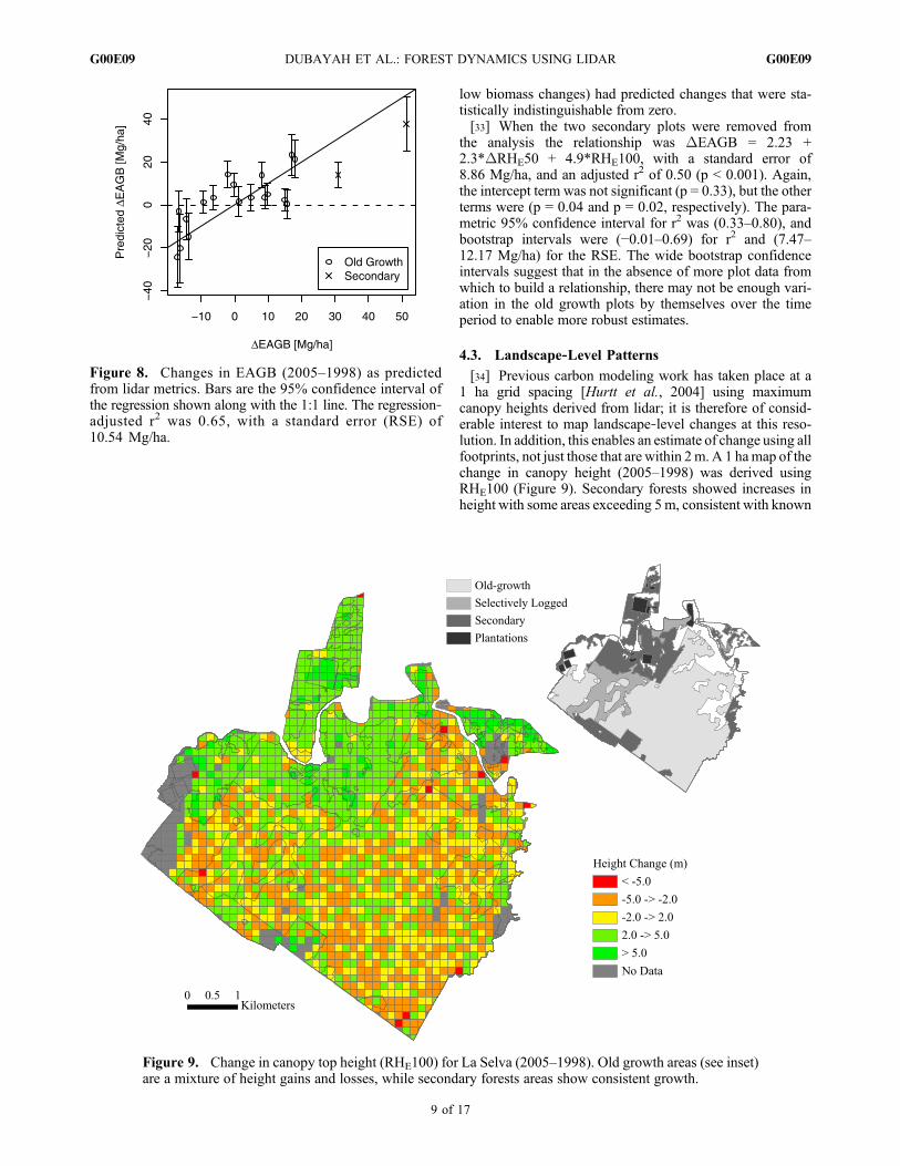
[34] Previous carbon modeling work has taken place at a1 ha grid spacing [Hurtt et al., 2004] using maximumcanopy heights derived from lidar; it is therefore of consid-erable interest to map landscape‐level changes at this reso-lution. In addition, this enables an estimate of change using allfootprints, not just those that are within 2m. A 1 hamap of thechange in canopy height (2005–1998) was derived usingRHE100 (Figure 9). Secondary forests showed increases inheight with some areas exceeding 5m, consistent with known

Figure 8. Changes in EAGB (2005–1998) as predictedfrom lidar metrics. Bars are the 95% confidence interval ofthe regression shown along with the 1:1 line. The regression‐adjusted r2 was 0.65, with a standard error (RSE) of10.54 Mg/ha.

Figure 9. Change in canopy top height (RHE100) for La Selva (2005–1998). Old growth areas (see inset)are a mixture of height gains and losses, while secondary forests areas show consistent growth.


9 of 17

rates of growth for younger forests at La Selva. In contrast oldgrowth forests were a mix of both height gain and loss.[35] The regression equation derived for combined sec-

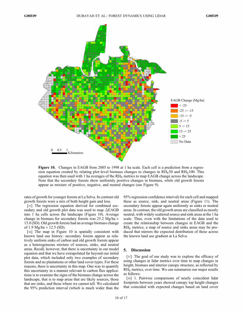
ondary and old growth plot data was used to map DEAGBinto 1 ha cells across the landscape (Figure 10). Averagechange in biomass for secondary forests was 25.2 Mg/ha ±15.0 (SD). Old growth forests had an average biomass changeof 1.9 Mg/ha ± 12.5 (SD).[36] The map in Figure 10 is spatially consistent with

known land use history: secondary forests appear as rela-tively uniform sinks of carbon and old growth forests appearas a heterogeneous mixture of sources, sinks, and neutralareas. Recall, however, that there is uncertainty in our modelequation and that we have extrapolated far beyond our initialplot data, which included only two examples of secondaryforests and no plantations or other land cover types. For thesereasons, there is uncertainty in this map. One way to quantifythis uncertainty in a manner relevant to carbon flux applica-tions is to examine the signs of the biomass change across thelandscape, that is to map areas that are likely sources, thosethat are sinks, and those where we cannot tell. We calculatedthe 95% prediction interval (which is much wider than the

95% regression confidence interval) for each cell andmappedthese as source, sink, and neutral areas (Figure 11). Thesecondary forests appear again uniformly as sinks or neutralareas. In contrast, the old growth areas are classified as mostlyneutral, with widely scattered source and sink areas at the 1 hascale. Thus, even with the limitations of the data used tocreate the relationship between changes in EAGB and theRHE metrics, a map of source and sinks areas may be pro-duced that mirrors the expected distribution of these acrossthe known land use gradient at La Selva.

5. Discussion

[37] The goal of our study was to explore the efficacy ofusing changes in lidar metrics over time to map changes inheight, biomass and interior canopy structure, as reflected byRHE metrics, over time. We can summarize our major resultsas follows:[38] 1. Pairwise comparisons of nearly coincident lidar

footprints between years showed canopy top height changesthat coincided with expected changes based on land cover

Figure 10. Changes in EAGB from 2005 to 1998 at 1 ha scale. Each cell is a prediction from a regres-sion equation created by relating plot‐level biomass changes to changes in RHE50 and RHE100. Thisequation was then used with 1 ha averages of the RHE metrics to map EAGB change across the landscape.Note that the secondary forests show uniformly positive changes in biomass, while old growth forestsappear as mixture of positive, negative, and neutral changes (see Figure 9).


10 of 17

types: plantations > secondary forests > selectively loggedforests > old growth forests[39] 2. Canopies that were shorter in 1998 had greater

probability of a transition to a taller canopy height class in2005. Conversely, canopies that were taller in 1998 hadtransition probabilities that were increasingly weightedtoward neutral changes in 2005.[40] 3. About 20% of the pairwise comparisons showed

height changes in excess of 5 m, with positive changesoutweighing negative ones.[41] 4. The lidar RHE100 and RHE50 metrics were linearly

related to biomass changes for combined old growth andsecondary forest plots, with an r2 of 0.65 and an RSE of10.5Mg/ha, but both parametric and bootstrapped confidenceintervals were wide, suggesting weaker model performance.[42] 5. Landscape‐level mapping at a 1 ha scale of canopy

height changes matched expected spatial patterns for thedistribution of land cover types at La Selva. Mean changeswere 0.57 m for all La Selva, and −0.33 m and 2.08 m forold growth and secondary forests, respectively.

[43] 6. Landscape‐level mapping at 1 ha scale of biomasschanges matched expected spatial patterns for the distributionof land cover types at La Selva. Mean changes were about25 Mg/ha for secondary forests and about 2 Mg/ha for oldgrowth forests.[44] 7. When prediction intervals were calculated to

classify 1 ha areas as biomass source and sinks, the resultingmap showed most of the old growth areas as neutral (statis-tically indistinguishable from zero), with widely scatteredand isolated sources and sinks. Secondary forests in contrastwere mostly sinks or neutral, but never sources.[45] To understand these results and place them in a

context for future analysis, both airborne and spaceborne,requires discussion of several issues relating to the limita-tions, errors and ultimate efficacy of the data and methodspresented. We begin by first noting that the experiment atLa Selva was arguably under some of the most difficultconditions that will be experienced. First, as will be dis-cussed, there were no large‐scale changes in structure andbiomass because there were no recent anthropogenic or

Figure 11. Map of sources, sinks, and neutral areas for La Selva. The 95% prediction interval was createdfor changes in EAGB. Those cells from Figure 10whose intervals were positive weremapped as sinks; thosethat were negative were mapped as sources. If the interval spanned zero, the cell was mapped as neutral.Secondary forests again appear uniformly as sinks or neutral areas, whereas old growth areas now appearmostly neutral with scattered source and sinks areas at the 1 ha scale.


11 of 17

natural disturbances. As a result there were no data on largenegative biomass changes, such as would occur throughdeforestation. Second, the majority of secondary forests wereat least 15 years into their recovery in 1998, so that the changein signal between years was not large on the positive side forcanopy structure and biomass at the landscape scale. Ourstudy also was limited by having only two secondary plots forbuilding a model relationship. Thus, we were left withchanges that were mostly related to isolated losses andincremental gains at the plot level.[46] One confounding aspect of our analysis was the

changes in apparent ground elevation experienced betweenyears. Our approach was to use the range measurements forcanopy top height changes instead of using heights foundrelative to the ground. Other change studies with LVIS havenot shown these apparent elevation differences in closedcanopy deciduous forests in the northeast United States andconifer forests in the western United States [O’Dell, 2006].Some ground finding errors are always present in lidar data,but these are generally rare enough that they do not limit theusefulness of lidar, even in tropical forests.[47] We hypothesized that the elevation errors seen

occurred in areas of high canopy cover or steep slopes.Both will weaken ground returns and hinder the accurateretrieval of ground elevation. Slope will also be a factor ifthe footprint comparisons have centers that are far apart (asthese will have truly different elevations, not just apparentelevation changes). There are a significant number of slopesthat exceed 10° at La Selva, however we found no statisticallysignificant relationship between slope and apparent elevationerror. A similar study in the rugged terrain of the SierraNevada of California found no relationship between errorsin LVIS heights versus field‐measured heights and slope aswell [Hyde et al., 2005]. We also found no relationshipbetween apparent elevation changes and canopy cover. Thedifficulty is that canopy cover, as derived from lidar, isexplicitly linked with finding the ground correctly (so thatthe relative energies in the canopy portion of the return andthe ground portion of the return may be found). Thoseareas that would have the highest canopy cover, and thusthe highest elevation errors, would also be the same oneswhere canopy cover was most in error as well, complicatingattempts to infer causation directly from the lidar data. Thus,we are unsure of the relative importance of each of the abovefactors for the appearance of ground finding errors in our datasets. We do know that there is a complex interaction betweensensor sensitivity, both spatially and vertically within foot-prints, canopy shape, canopy structure and topography thatwill require more research to resolve for relevance to changestudies.[48] The issue of validation of lidar‐derived height changes

is a difficult one. We did not have field‐validated changes inheight for both years. As discussed, the 1998 heights werevalidated by Peterson [2000] who found accuracies that werecomparable to other lidar studies [e.g., seeMeans et al., 1999;Hyde et al., 2005; Anderson et al., 2006] that have generallyshown height retrieval accuracies in the 3–5 m range, butmuch of the reported error may be attributable to the diffi-culties in accurately determining height from the ground (adaunting task in closed canopy forests). Small‐footprintdata may be used as a type of validation for canopy heightand more directly, for canopy top elevation (height above

ellipsoid) as shown in Figure 3. The use of small‐footprint lidarfor validation assumes that these data are correct or otherwisevalidated. Again, such validationmay not be simple, especiallywhen multiple platforms acquire observations separated intime, as biases and errors may creep into the process at severalpoints. The great advantage of space‐based missions, such asDESDynI, is that they provide stable measurement platformsthat allow for more direct intercomparison of data sets withina common observational framework.[49] What do our results tell us about the magnitude of

canopy height changes required for detection as a functionof the spatial scale of observation? Validations of heightmight suggest 3–5 m as these brackets commonly reportedaccuracies from field studies. However, these may be tooconservative because of the difficulties of field validation.[50] Measuring changes in the range to canopy top

(RHE100) may be more accurate than measuring heights (asdone in field studies). For example, consider a 0.5 m2 panel ofleaf material (about the minimum detectable area for LVIS),oriented horizontally. LVIS would measure changes in therange to this panel with centimeter to tens of centimeters‐level accuracy. This repeatability of successive height mea-surements is essentially random measurement error and whatwe would characterize as instrument error.[51] If canopies were composed of architectures like these,

decimeter accuracies for changes in height using RHE100would be achievable. However, canopy architectures and theenvironments they occur in are variable and lead to heighterrors that are not easily categorized as “instrument error.”Slopes accentuate pointing errors that lead to errors in thehorizontal locations of the range measurements, and thus inturn to errors in the absolute vertical elevations of returnsused to find differences in elevation. The systematic errorsin pointing are generally accounted for and are included inthe instrument error. Random errors in pointing do occur aswell, however. Slopes may produce additional errors thatmay be viewed as some combination of both systematic andrandom. Consider a 25 m footprint with an even heightstand on a slope. The instrument will systematically measurethe range to trees that occur at the edge of the upslopeportion of the footprint. As long as trees grow uniformly inthe entire footprint over time, a difference of ranges removethis effect. If trees do not grow uniformly, or if the stand hasan uneven height structure within the footprint, then errorsin range difference will occur.[52] Canopy architecture and its changes over time are

another source of error. Pointing errors are less important forflat canopies than they are for steep‐sided canopies, such asconifer forests. This could then translate into errors in rangeretrieval as a function of forest type. Changes in canopyarchitecture over time can also be important. For example, ifa canopy becomes more closed over time so that there is lesspenetration of the beam into the canopy, the change in rangemay be inferred as growth, when actually none occurred.[53] Attributing these types of errors, whether from slope

or canopy conditions into instrument or environmental, andinto random or systematic, is difficult because of the inter-actions that occur between sensor and the landscape, but isthe subject of continued study. However, the distinctionbetween random and systematic errors is important becausethe former can be overcome by increased sampling, as willbe discussed, but the latter leads to a bias that cannot.


12 of 17

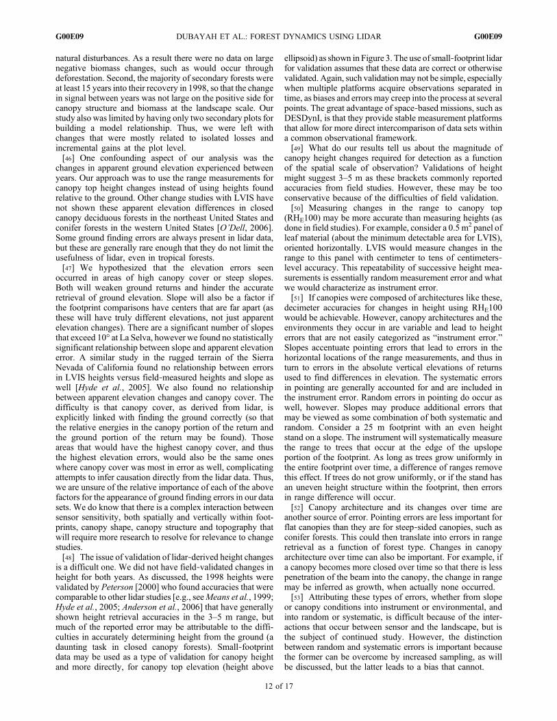
[54] Thus, characterizing the magnitude of the changesrequired for detection is complex. For footprint‐to‐footprintcomparisons, the most conservative answer is to assume that(1) field‐based estimates of height errors are correct, and(2) the errors are not random between years, so that theerrors do not cancel when calculating a change. In this worsecase, an estimate of the expected error would be s = √(s12 + s22),where s1 and s2 are the overall validation errors from eachyear. So within year errors of 3–5 m would yield RMS errorsof about 4–7 m. However, this is overly conservative, espe-cially for mission design, as it conflates errors in field mea-surements, sensor errors and their interaction with canopy andenvironmental conditions. A more reasonable estimate forwithin year errors is likely around 1–2 m, which would yieldRMS errors of about 1.5–3 m. This suggests that changesmight need to exceed this range to be detectable by an indi-vidual footprint‐to‐footprint comparison between years.[55] As we increase to the 1 ha scale and beyond, sam-

pling issues arise and our errors will also now be a functionof how many observations are available. We have moreobservations in a cell from which to calculate a cell mean fora particular year than we do footprints between years thatare coincident. We can thus calculate a difference of meansbetween years using all the observations that fall within acell. To determine if there is a difference in the mean canopyheight requires that we have an estimate of the height var-iance at that scale, an estimate of sensor error, and sufficientnumbers of observations. We have a variance contributed bythe natural variability of the landscape and that induced by

sensor measurement error. An estimate of the variance in aparticular year is sTOTAL

2 = (ssensor2 + sheight

2 ), where ssensor isour estimated sensor measurement error and sheight is theheight variability within a cell. The second term, sheight, mayalso include the interaction of sensor pointing variabilitywith the spatial variability of canopy height (a variation inpointing on a homogenous canopy will exhibit no heightvariance, whereas the same variation on spatially varyingcanopy will produce an additional height variance compo-nent). Alternately, this type of interaction could be book keptas an additional error term in the equation given above. Theaverage RHE100 (canopy top) variability at La Selva variedas a function of cell size and location, with a mean value ofabout 6 m at the 1 ha scale and was constant between years.If we assume an average sensor error of about 2 m (in themiddle of our 1.5–3 m range above), the total variability issTOTAL = 6.3 m. This number expresses the combineduncertainty of the measurement process and the samplingprocess.[56] The height requirement for DESDynI observations

within cells of varying size is that the estimate of the meanmust be within 1 m about 68% of the time (i.e., ±1 standarddeviation and referred to as a “one meter, one sigma”requirement). The error associated with a difference of means,assuming the same number of observations and the sametotal variability in each year for simplicity, can be expressedas d = ±ta* √(2sTOTAL2 /n), where d is the error or detectabledifference, ta is the t statistic for a given significance level,and n is the number of observations in a given year.[57] We can vary the magnitude of sTOTAL to approxi-

mate the required sample size (number of lidar observations)to detect a specific height change d under the same assump-tions as given above. Figure 12 shows the relationship forsTOTAL ranges from 4–14 m, and with t ≈ 1 (as in theDESDynI requirement). As can be seen the number ofobservations required to get relatively small errors (andthus small detectable changes) is large. If we assume wehave an 8 m variability and 16 observations, say in a 1 hacell, the error would be ±2.93 m. For the greater than 5000observations of footprint pairs we have for La Selva ourestimate of the difference of means for the entire landscapebetween years should be accurate to within ±0.13 m. If sensorerror can be shown to be closer to 1 m, then these accuracieswould increase and the number of observations requiredwould decrease. Likewise, fewer observations would berequired for more even‐aged stands that have smallerspatial variability. Note that systematic errors or biases arenot necessarily removed by increased sampling. A morecomplete analysis of errors would include an n and sTOTALthat vary in each observation year, as well as a desired levelof b or “Type II” error, in addition to the a level, to determinea priori the required numbers of observations to detect achange of a given level. Such an analysis would also includemodeling the effects of using nonpoint (areal lidar footprint)sampling on spatially autocorrelated fields of height struc-ture, but is beyond our scope here.[58] Assigning an error to the other RHE change metrics is

not easily done using field observations. Our approach is toassume these have small errors when expressed in elevationspace. As discussed earlier, the waveform as defined by itsvertical extent is a fundamental measurement that gives therecord of intercepted surfaces. Errors appear when the

Figure 12. Number of lidar observations required to detecta given difference of mean canopy height within an area.Each line gives the total variability sTOTAL (within cell heightvariability and sensor error) varying from 4 to 14 m (frombottom line to top line). For example, with sTOTAL = 4 m,a change in mean of ±1 m would require about 30 observa-tions. Note the logarithmic scale on the x and y axes.


13 of 17

waveform is interpreted, and such interpretation is minimal ifthe waveform is kept in elevation space. In practice, however,most users would prefer RH metrics interpreted as a heightabove the ground, and thus any errors in ground finding mayagain appear. There has been little evaluation of the effects ofgeolocation errors, topography, off‐nadir pointing, and can-opy penetration on these metrics, either for RH or RHE. If theuse of these metrics for change analysis continues, studiesshould be done that attempt to define their accuracy relative tovertical canopy structures.[59] We developed two linear regression equations to

predict biomass change. Their form was consistent, withthe coefficient for DRHE100 about twice that for DRHE50.The intercept term was rather large, but statistically notsignificant. The equations, as models of the relationshipsbetween canopy structure variables and biomass are physi-cally reasonable. As canopies grow and accumulate biomasswe expect both variables to positively increase. The oppositeis also true: as biomass decreases, both of these metrics willdecrease. However, it is possible, as our model suggests, tohave alternate signs for these variables, and depending ontheir magnitude, achieve either a positive, negative or neutralchange in biomass. To a first approximation, changes incanopy top height must be related to changes in biomass; it ismore likely that large changes in this height will lead tochanges in biomass than it is these height changes will occurbut that biomass stays the same. This would happen if positiveor negative changes in RHE50 take place that are approxi-mately twice that of the RHE100, but have opposite signs. Ifthe changes in RHE50 are large enough relative to RHE100,they will drive the biomass toward the direction of that

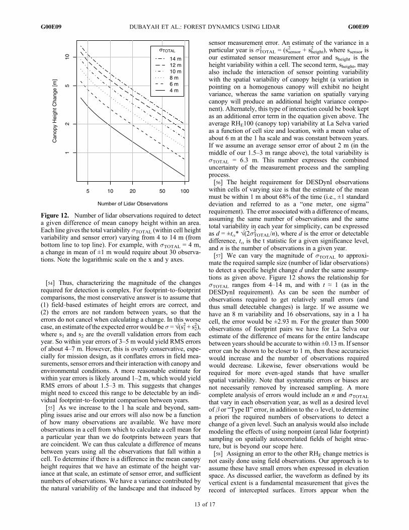
change. How these changes occurred at La Selva is givenessentially in Figure 10, which maps our regression equationusing the actual cooccurrences of DRHE50 and DRHE100.At the 1 ha scale, positive/positive changes (both DRHE100andDRHE50 are positive, respectively) occurred 50% of thetime; negative/negative changes occurred 28% of the time;negative/positive and positive/negative changes occurred ata frequency of 12% and 10%, respectively. This suggeststhat it is far more likely for changes in both metrics to occurin the same direction (78% of time). It further suggests thatfor the landscape of La Selva, the most likely changes instructure were positive for both metrics. This is a reasonableresult given the area of secondary forests and plantations. Wefind similar results at the footprint scale as well: 68% of thechanges were in the same direction with 43% positive‐positive. Figure 13 shows the relationship of these metricsto biomass changes for the 20 plots used in our study.[60] The small number of total plots and limited number

of secondary plots hindered the development of our combinedold growth/secondary regression equation. Our equation didnot predict the secondary changes well. One secondary plot,“lep” (see Table 1), had low values for both DRHE100 andDRHE50 (0.58 m and 1.7 m) even though the change inbiomass was large (31 Mg/ha). The reason for this, discussedearlier, was that the plot was not sampled uniformly eachyear. In 2005 only about 1 half of the plot had usable lidarreturns, and this half was composed of taller trees that did notgrow as much as the half that was not sampled again. Theresult was little change in metrics as compared to the othersecondary plot and even some old growth plots.[61] Judging from Figures 8 and 13, small changes in

biomass were difficult to model at the plot scale. This wasreinforced by the weaker regression relationship found usingonly old growth plots. This may be because such changes atthe scale of 0.5 to 1 ha plots may occur from many smallchanges in canopy structure, each of which is hard to detect.A forest far along in its successional trajectory may accu-mulate biomass slowly, with occasional mortality events. Ascan be seen from the height transition matrix (Table 2), 25 mfootprints detect these changes at the footprint level acrossLa Selva (for 5 m height classes, many transitions awayfrom the previous height class occurred), but averagechanges to these metrics at the plot scale may be difficult toestablish accurately unless the changes are large. The metricsfor many plots used in this study had relatively small (0–2 m)changes over the 7 year period. For the 0.5 ha Carbonoplots it seems unlikely that average changes less than 2 m inRHE100 are detectable by LVIS based on our error analysis.[62] The regression equations themselves had RSE values

(around 10Mg/ha) that were significant fractions or exceededin some cases the magnitude of the changes being modeled,with the exception of the secondary plots. Because of theselarge errors, we explored whether the lidar data could at leastbe used to map source and sink areas with confidence. Ourresults suggest that maps of source/sink areas inferred fromlidar growth changes are possible at the 1 ha scale. Using the95% prediction interval to find cells with biomass changessignificantly different from zero gave spatially meaningfulresults that matched known land use types. Again, thechanges observed at the plot level were not large at La Selvabecause of the lack of recent disturbance and recovery. If theold growth forest biomass change rates at La Selva are rep-

Figure 13. Relationship between changes in RHE100 andRHE50 heights and EAGB for the Carbono and secondaryforest plots. The vertical line gives the distance betweenthe changes in RHE100 and RHE50, and the symbols givethe change for that particular metric. The signs of the changesare generally the same: when both metrics are positive, bio-mass change is positive, and vice versa. Note that often thechange in RHE50 was larger than that for RHE100. Addition-ally note the small changes (less than 2 m) in the metrics formany of the plots. The secondary plot “lep”was incompletelysampled and has metric changes that are not representative.


14 of 17

resentative of the tropics as a whole, it may be difficult to gobeyond source/sink designation and quantitatively assessaccumulation and loss over these forests if they are under-going no changes other than normal mortality and growth atthe 1 ha scale. If footprint based biomass equations can bedeveloped with suitable accuracy (as in the work of Drake etal. [2002a]), footprint‐scale changes may be easier to assess.As the scale gets even smaller (as in the work of Kellner et al.[2009]), changes should be even more evident.[63] Our results as compared with those of Kellner et al.

[2009] show differences, such as the percentages of areasundergoing positive versus negative changes. These may beattributed to the nonidentical domains of analysis, with ourstudy including land cover types other than old growth.Others may have to do with the differences in spatial scaleof the lidar footprints and subsequent aggregation scales. Forexample, we found higher probabilities of canopy observa-tions remaining in the same height class between years (i.e.,the diagonal of Table 3 has higher probabilities). One reasonfor this may be that canopy changes at the 5 m scale, inparticular gaps, are either too small or otherwise average outat 25 m scales, and thus are harder to detect. Interestingly, wefound identical changes in canopy height (DRHE100) for oldgrowth forests (−0.33 m) as Kellner et al. [2009] who report−0.32 m, even though different definitions of height wereused. Kellner et al. [2009] calculated the average heightabove ground of all lidar returns within 5m cells for each yearand subtracted these. For canopies that are somewhat open,using an average height derived from small footprint lidar willresult in a mean height that is below the top of the canopy asreturns will go back to the sensor from the entire depth ofcanopy.With larger footprint systems, there will also be somepenetration into the canopy until enough signal is generated toget above the noise level. That these two different types ofmeasurements using different definitions of height observedan identical change is not intuitive. We doubt, though it ispossible, that such close agreement is by chance. Oneexplanation may lie with the canopy structure of the oldgrowth forests at La Selva. These forests are quite closed andmuch of the leaf material is concentrated near the top of the

canopy [Clark et al., 2008]. Thus a small‐footprint systemutilizing a last‐return technology would have many of itsreturns from the outer canopy surface.We also note that LVISwas biased low (−0.43 m, see Figure 3) relative to small‐footprint maximum returns within LVIS footprints, suggest-ing that some canopy penetration may have occurred withLVIS (however, this difference may also have been caused bydry season leaf drop during the LVIS acquisition). It may bethen, that for these closed forests, average small‐footprintheight and LVIS canopy top heights are similar enough, thatwhen averaged over thousands (in the case of LVIS) andhundreds of thousands of observations (in the case of Kellneret al. [2009]), the same average change is measured. Thistheory potentially could be tested by following the method ofBlair and Hofton [1999] that creates “pseudowaveforms”from small footprint data. Pseudowaveforms could becreated for each year and changes in these compared tochanges observed by LVIS.[64] The magnitude of changes in biomass mapped spa-

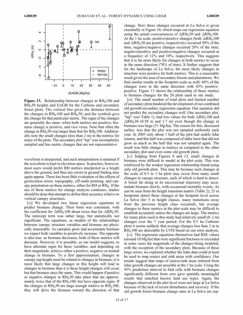
tially at fine scales provides important information for futurespace missions, such as DESDynI, whose central goals includeobserving changes in biomass. We have limited knowledgeof the spatial and temporal variability of such changes acrossthe globe. Efforts using airborne lidar such as presented herecan help provide this information. In addition, these types ofresults serve as benchmarks for establishing and predictingmission performance. Science considerations have estab-lished a DESDynI accuracy requirement for biomass changesof ±2–10MgC/ha/y (or 20%, whichever is larger) annually at500 m to 1000 m resolution. The largest of these changes,and most important, will be from deforestation events and thesubsequent rapid regrowth that occurs within a nominal5 year mission length. However, the changes associatedwith small‐scale disturbance, such as mortality events, andlater stages of regrowth may be more difficult to detect. AtLa Selva there have been no recent large‐scale disturbances(and the magnitude of changes present there reflect this). Forexample, in 2000, only about 95 ha of secondary forest out ofthe 1600 ha of La Selva were in the age class of 1–12 years.The remaining 250 ha of secondary forest were in the ageclass of 13–34 years, well into their recovery period. There-fore, only a small portion of La Selva observed in 1998 byLVIS was recently (<5 years) disturbed. Only eight of the18 Carbono plots exceeded the rate of 2 Mg/ha/yr accordingto field‐based estimates (Table 1), and only one exceeded2.5 Mg/ha/yr. Assuming 50% of the change of biomass iscarbon, none of the plots had rates that would be detectedby DESDynI.[65] We can get an approximate sense of the rate of

change across the landscape by using the predictions shownin Figure 10. About 20% of the 1 ha cells had rates thatexceeded 2 MgC/ha/yr (Figure 14). This is an uncertainestimate however, because of the errors in the regressionequation used to estimate change. If we use a 95% predictioninterval again, we can be certain that only 30 cells had rangesthat exceeded the DESDynI requirement, and of these onlyone was negative. This does not mean that such changes didnot occur, only that we cannot confidently predict these rateswith the data used in this study. Nonetheless, the combinationof our model results along with the actual changes measuredin the field suggests rates of change below what DESDynIwill measure, except for secondary forests and other rapidly

Figure 14. Estimated rates of change in aboveground car-bon for 1 ha cells. The dashed vertical lines give the lowerchange requirement for DESDynI (2 MgC/ha/yr).


15 of 17

changing land cover types. However, the very fact that suchareas would appear neutral under DESDynI observationswould identify these forests as likely old growth areas, andwhen taken together with the larger changes associated withdisturbance and regrowth, should enable a greatly improvedaccounting of the flux of carbon between the land surfaceand the atmosphere.[66] Another aspect of our study with relevance to DES-

DynI is that more variability was observed when footprintlevel changes are estimated (Table 3 and Figure 7) as opposedto averages over plots. DESDynI will have billions of“crossovers,” places on the Earth where orbital paths crossand footprints overlap. The planned geolocation accuracy is10 m, on average. Even though many of these footprint pairswill be much closer together than 10 m, we may not have aposteriori knowledge of the distance between specific foot-print pairs to better than this distance. Nonetheless, these willprovide valuable information on mortality rates and heightdynamics. As we look at slightly larger areas around thecrossover points, geolocation errors become less important,and the increased numbers of observations will enable moreaccurate determination of change within these.[67] Last, some consideration must be given to the diffi-

culties of field validation. We have already discussed issuesrelated to validation of lidar remote sensing. A much largerproblem exists with the validation of biomass. In tropicalregions all such field estimates are done via generalizedallometric equations that are derived from a remarkablylimited number of trees. This problem is well known butwidespread: no study that aims to predict tropical biomass canavoid it. The precision of biomass estimates at La Selva ishigh, so that year‐to‐year changes should be well character-ized. But there remains the possibility that lidar capturesstructure that is well related to biomass and biomass changes,but that the dbh‐based allometries are in error, and thereforelidar model failures to accurately predict changes actuallymay be failures to match another model’s estimates that initself has errors of the same magnitude.[68] A solution to this problem is better allometry. Field‐

based estimates of biomass will be essential to relate globalobservations of structure from DESDynI to biomass andimproved allometry is key. Additionally, a global networkof plot data is required. This is especially true for biomassdynamics. There are very few sets of permanent plots similarto the Carbono project globally, yet even this unmatched dataset was not ideal because the range of biomass changes wasnarrow, and consequently limited our analysis. Even if bio-mass changes are found by year‐to‐year differences of bio-mass in DESDynI, these will require actual measurements ofchange for validation and error analysis. In the coming years,if methodologies such as presented here can be improved andextended, then limited field data can be used with airbornelidar data to make spatially extensive maps of change indifferent biomes that can then be used to both calibrate andvalidate measurements from DESDynI.

6. Conclusion

[69] Our results at La Selva reveal a landscape underconstant change as a result of growth, mortality, recruitment,and recovery from disturbance. When the effects of anthro-pogenic changes are superimposed, along with climatic and

edaphic factors, determining the true successional status of alandscape required for accurate estimation of carbon stocks,fluxes and other ecosystem functions is a daunting challenge.Our basic premise in initiating this research was that inferenceof successional state and measurement of net terrestrial car-bon flux between the land surface and the atmosphere may beapproached by directly observing changes in canopy structureover time. This would enable the spatial mapping and quan-tification of the magnitudes of carbon source and sink areas.However, because spatially explicit maps of canopy andbiomass dynamics over tropical forests at fine scales are rare,the ability of lidar and other remote sensing technologies tocapture this variability over relatively short time spans andwithin their measurement accuracies was unknown. Theworkpresented here suggests that lidar remote sensing is a viablemethod for quantifying short‐term tropical forest dynamics.While changes in old growth biomass may be hard todetect at the plot scale over these time spans because theyare small, larger changes associated with disturbance andrecovery should be measureable. Even over slowly evolvingold growth forests, footprint‐level changes in canopy struc-ture associated with small‐scale disturbance, mortality andregrowth are observable. The ability of lidar to capture tran-sitions across the entire spectrum of canopy structure andheight is unprecedented and will provide a valuable new toolfor deepening our understanding of how forest structuresrespond through time to changes in land use and climate.[70] Our results also suggest that the mission concept of

DESDynI, combining both lidar and radar to observe sourceand sink dynamics from space should be effective in mea-suring the larger changes in biomass for which it is designed:those that occur from deforestation and subsequent regrowth.The combination of the spatially complete coverage of radarand the tens of billions of detailed lidar profiles expectedfrom the DESDynI should revolutionize our understandingof forest dynamics and its effect on carbon cycling andhabitat structure.

[71] Acknowledgments. This work was supported by grants fromNASA’s Terrestrial Ecology and Interdisciplinary Science Programs(R. O. Dubayah) and a NASA Earth System Science Graduate Fellowship(S. L. Sheldon). Monitoring of the CARBONO plots was supported by theTEAM Project of Conservation International, made possible with a grantfrom the Gordon and Betty Moore Foundation, and the National ScienceFoundation (LTREB 0841872). Monitoring of the secondary plots wassupported by grants from the Andrew W. Mellon Foundation, the NationalScience Foundation, and the University of Connecticut Research Founda-tion. We thank two anonymous reviewers for useful comments on the man-uscript, and especially Jim Kellner for valuable discussions on our work.

ReferencesAnderson, J., M. E. Martin, M. L. Smith, R. O. Dubayah, M. A. Hofton,and P. Hyde (2006), The use of waveform lidar to measure northern tem-perate mixed conifer and deciduous forest structure in New Hampshire,Remote Sens. Environ., 105(3), 248–261, doi:10.1016/j.rse.2006.07.001.

Blair, J. B., and M. A. Hofton (1999), Modeling laser altimeter return wave-forms over complex vegetation using high‐resolution elevation data, Geo-phys. Res. Lett., 26(16), 2509–2512, doi:10.1029/1999GL010484.

Blair, J. B., D. L. Rabine, and M. A. Hofton (1999), The laser vegetationimaging sensor (LVIS): A medium‐altitude, digitization‐only, airbornelaser altimeter for mapping vegetation and topography, ISPRS J. Photo-gramm. Remote Sens., 54, 115–122, doi:10.1016/S0924-2716(99)00002-7.

Brown, S. (1997), Estimating biomass and biomass change of tropical forests:A primer, FAO For. Pap. 134, Food and Agric. Org., Rome, Italy.

Chazdon, R. L., S. G. Letcher, M. van Breugel, M. Martinez‐Ramos,F. Bongers, and B. Finegan (2007), Rates of change in tree communities


16 of 17

of secondary Neotropical forests following major disturbances, Philos.Trans. R. Soc. London, Ser. B, 362, 273–289, doi:10.1098/rstb.2006.1990.

Clark, D. A. (2004), Tropical forests and global warming: slowing it downor speeding it up?, Front. Ecol. Environ, 2(2), 73–80.

Clark, D. B., and D. A. Clark (1996), Abundance, growth and mortality ofvery large trees in neotropical lowland rain forest, For. Ecol. Manage.,80, 235–244, doi:10.1016/0378-1127(95)03607-5.

Clark, D. B., and D. A. Clark (2000), Landscape‐scale variation in foreststructure and biomass in a tropical rain forest, For. Ecol. Manage.,137, 185–198, doi:10.1016/S0378-1127(99)00327-8.

Clark, D. B., P. C. Olivas, S. F. Oberbauer, D. A. Clark, and M. G. Ryan(2008), First direct landscape‐scale measurement of tropical rain forestLeaf Area Index, a key driver of global primary productivity, Ecol. Lett.,11, 163–172.

Clark, M. L., D. B. Clark, and D. A. Roberts (2004), Small‐footprint lidarestimation of sub‐canopy elevation and tree height in a tropical rain forestlandscape, Remote Sens. Environ., 91, 68–89, doi:10.1016/j.rse.2004.02.008.

Donnellan, A., H. Zebker, and K. J. Ranson (2008), Radar and lidar mea-surement of terrestrial processes, Eos Trans. AGU, 89(38), doi:10.1029/2008EO380002.

Drake, J. B., R. O. Dubayah, D. B. Clark, R. G. Knox, J. B. Blair,M. A. Hofton, R. L. Chazdon, J. F. Weishampel, and S. Prince (2002a),Estimation of tropical forest structural characteristics using large‐footprintlidar, Remote Sens. Environ., 79, 305–319, doi:10.1016/S0034-4257(01)00281-4.

Drake, J. B., R. O. Dubayah, R. G. Knox, D. B. Clark, and J. B. Blair(2002b), Sensitivity of large‐footprint lidar to canopy structure and bio-mass in a neotropical rainforest, Remote Sens. Environ., 81, 378–392,doi:10.1016/S0034-4257(02)00013-5.

Drake, J. B., R. G. Knox, R. O. Dubayah, D. B. Clark, R. Condits, J. B. Blair,and M. A. Hofton (2003), Above‐ground biomass estimation in closedcanopy Neotropical forest using lidar remote sensing: Factors affectingthe generality of relationships, Global Ecol. Biogeogr., 12, 147–159.

Dubayah, R., et al. (1997), The Vegetation Canopy Lidar mission, in LandSatellite Information in the Next Decade, vol. 2, pp. 100–112, Am. Soc.for Photogramm. and Remote Sens., Washington, D. C.

Duong, V. H., R. Lindenbergh, N. Pfeifer, and G. Vosselman (2008), Singleand two epoch analysis of ICESat full waveform data over forested areas,Int. J. Remote Sens., 29(5), 1453–1473, doi:10.1080/01431160701736372.

Hartshorn, G. S., and B. E. Hammel (1994), Vegetation types and floristicpatterns, in La Selva: Ecology and Natural History of a Neotropical RainForest, edited by L. A. McDade et al., pp. 73–89, Univ. of ChicagoPress, Chicago, Ill.

Hofton, M. A., and J. B. Blair (2002), Laser altimeter return pulse correla-tion: A method for detecting surface topographic change, J. Geodyn., 34,477–489, doi:10.1016/S0264-3707(02)00043-1.

Hofton, M. A., L. E. Rocchio, J. B. Blair, and R. Dubayah (2002), Valida-tion of Vegetation Canopy Lidar sub‐canopy topography measurementsfor a dense tropical forest, J. Geodyn., 34, 491–502, doi:10.1016/S0264-3707(02)00046-7.

Hofton, M. A., R. Dubayah, J. B. Blair, and D. Rabine (2006a), Validationof SRTMelevations over vegetated and non‐vegetated terrain usingmediumfootprint lidar, Photogramm. Eng. Remote Sens., 72(3), 279–285.

Hofton, M. A., E. Malavassi, and J. B. Blair (2006b), Quantifying recentpyroclastic and lava flows at Arenal Volcano, Costa Rica, using medium‐footprint lidar, Geophys. Res. Lett. , 33 , L21306, doi:10.1029/2006GL027822.

Houghton, R. A., and S. J. Goetz (2008), New satellites help quantify carbonsources and sinks, Eos Trans. AGU, 89(43), doi:10.1029/2008EO430001.

Houghton, R. A., K. T. Lawrence, J. L. Hackler, and S. Brown (2001), Thespatial distribution of forest biomass in the BrazilianAmazon: A comparisonof estimates, Global Change Biol., 7, 731–746, doi:10.1046/j.1365-2486.2001.00426.x.

Hurtt, G. C., R. Dubayah, J. Drake, P. R. Moorcroft, S. W. Pacala, J. B.Blair, and M. G. Fearon (2004), Beyond potential vegetation: Combininglidar data and a height‐structured model for carbon studies, Ecol. Appl.,14(3), 873–883, doi:10.1890/02-5317.

Hyde, P., R. Dubayah, B. Peterson, J. B. Blair, M. Hofton, C. Hunsaker,R. Knox, and W. Walker (2005), Mapping forest structure for wildlifehabitat analysis using waveform lidar: Validation of montane ecosystems,Remote Sens. Environ., 96(30), 427–437, doi:10.1016/j.rse.2005.03.005.

Kellner, J. R., D. B. Clark, and S. P. Hubbell (2009), Pervasive canopydynamics produce short‐term stability in a tropical rain forest land-scape, Ecol. Lett., 12, 155–164, doi:10.1111/j.1461-0248.2008.01274.x.

Lefsky, M. A., W. B. Cohen, G. G. Parker, and D. J. Harding (2002), Lidarremote sensing for ecosystem studies, BioScience, 52(1), 19–30,doi:10.1641/0006-3568(2002)052[0019:LRSFES]2.0.CO;2.

Lefsky,M. A., D. Harding,M. Keller,W. B. Cohen, C. Carabajal, F. DelBomEspirito‐Santo, M. O. Hunter, and R. de Oliveira Jr (2005), Estimates offorest canopy height and aboveground biomass using ICESat, Geophys.Res. Lett., 32, L22S02, doi:10.1029/2005GL023971.

McDade, L. A., K. S. Bawa, H. A. Hepensheide, and G. S. Hartshorn(1994), La Selva: Ecology and Natural History of a Neotropical RainForest, Univ. of Chicago Press, Chicago, Ill.

Means, J. E., et al. (1999), Use of large‐footprint scanning airborne lidar toestimate forest stand characteristics in the Western Cascades of Oregon,Remote Sens. Environ., 67(3), 298–308, doi:10.1016/S0034-4257(98)00091-1.

Naesset, E., and T. Gobakken (2005), Estimating forest growth using canopymetrics derived from airborne laser scanner data, Remote Sens. Environ.,96, 453–465, doi:10.1016/j.rse.2005.04.001.

O’Dell, K. (2006), Estimating changes in forest height and structure inHubbard Brook Experimental Forest using lidar remote sensing, M.A.scholarly paper, Univ. of Md., College Park.

Peterson, B. (2000), Recovery of forest canopy heights using large‐footprintlidar, 58 pp., M.A. thesis, Univ. of Md., College Park.

Thomas, R. Q., G. C. Hurtt, R. O. Dubayah, and M. H. Schilz (2008), Usinglidar data and a height‐structured ecosystem model to estimate forest car-bon stocks and fluxes over complex mountainous terrain, Can. J. RemoteSens., 2(34), S351–S363.

J. B. Blair, Laser Remote Sensing Laboratory, NASA Goddard SpaceFlight Center, Greenbelt, MD 20771, USA.R. L. Chazdon, Ecology and Evolutionary Biology, University of

Connecticut, Storrs, CT 06269, USA.D. B. Clark, Department of Biology, University of Missouri at St. Louis,

R223 Research Bldg., Saint Louis, MO 63121, USA.R. O. Dubayah, M. A. Hofton, and S. L. Sheldon, Department of

Geography, University of Maryland, Lefrak Hall, College Park, MD20742, USA. ([email protected])G. C. Hurtt, Institute for the Study of Earth, Oceans, and Space,

University of New Hampshire, Morse Hall, Durham, NH 03824‐2600,USA.


17 of 17

Date post:	21-May-2018
Category:	Documents
Upload:	trinhngoc
View:	215 times
Download:	0 times

Estimation of tropical forest height and biomass dynamics ...biology/files/pdfs/dave-clark/Dubayah...

Documents