Estimation of Wind Speed and Shear on Wind...

Estimation of Wind Speedand Shear on Wind TurbinesEstimation of Wind Speed and Shear on Wind Turbines

Gr 1030 Electronics & ITControl and Automation

Aalborg University06-06-2013

E10 PROJECTE10 PROJECT

Department of Electronic systemsElectronics & ITFredrik Bajers Vej 79220 Aalborg ØTel. 99 40 86 00www.sict.aau.dk

Title:Estimation of Wind Speed andShear on Wind Turbines

Subject:Master thesis

Project period:February 4th - June 6th, 2013

Group:Group 1030

Group members:Mikkel Urban KajgaardJesper MogensenAnders Wittendorff

Supervisors:Rafael WisniewskiChristoffer Sloth

Copies: 6

Page count: 123

Attachments: CD

Appendices: 4

Completion: June 6th 2013

Synopsis:

The goal for this project has been todevelop a wind turbine model describ-ing the deflections and displacements ofthe physical and mechanical parts as afunction of incident wind for a 5 MW

wind turbine. An estimator for estimat-ing wind by terms of hub height windspeed and vertical shear should also bedesigned. An LPV model has beenpartly derived, in the means of statingthe principles. However, not all of theterms necessary to express the modelbehaviour by means of system matri-ces describing mass, stiffness and damp-ing, have been derived due to the timelimitations of the project period. Themodel is instead tested and validatedwith system matrices from a rotor angledependent linearisation, obtained fromthe NREL FAST toolbox for MATLAB.The model is validated against simula-tions using this toolbox as well. The de-rived model shows potential when simu-lated against the non-linear model fromFAST, but deviates when the inputs de-viates from the operating points. A lin-earised Kalman estimator has been de-signed, which estimates the two windparameters subjected to process- andmeasurement noise with a mean devi-ation of respectively 1.22 % and 0.33 %.

The content of this report is freely available however, publication (with reference) may only happenper agreement with the authors.

Institut for Elektroniske SystemerElektronik og ITFredrik Bajers Vej 79220 Aalborg ØTlf. 99 40 86 00www.sict.aau.dk

Titel:Estimering af Vindhastighed og Vin-dgradient på Vindmøller

Tema:Speciale afhandling

Projekt periode:4. februar - 6. juni, 2013

Gruppe:Gruppe 1030

Gruppemedlemmer:Mikkel Urban KajgaardJesper MogensenAnders Wittendorff

Vejledere:Rafael WisniewskiChristoffer Sloth

Antal oplag: 6

Antal sider: 123

Bilag: CD

Appendikser: 4

Afsluttet: 6. juni, 2013

Synopsis:

Målet for dette projekt har været at ud-vikle en vindmøllemodel der beskriverbøjninger og forskydninger af de fy-siske og mekaniske dele som funktion afden indfaldende vind for en 5 MW vind-mølle. En estimator til at estimere vindi form af vindhastighed i navhøjde ogvertikal gradient skulle også designes.En LPV model blev delvist udledt, iform af fastsættelse af principper forudledninger. Dog, blev ikke alle nød-vendige udtryk til beskrivelse af mod-ellens opførsel i form af system ma-tricer for masse, stivhed og dæmpn-ing udledt, grundet projektperiodenstidsbegrænsning. Modellen er istedettestet og valideret med system ma-tricer fra en rotorvinkel-afhængig lin-earisering, udvundet fra NREL FASTværktøjet til MATLAB. Modellen erligeledes valideret ved simuleringer meddette værktøj. Den udledte model viserpotentiale når den simuleres mod denulineære model i FAST, men afviger nårstyringssignalerne afviger fra arbejd-spunkterne. En lineariseret Kalman es-timator er blevet designet, der udsat forprocessstøj estimerer de to vindparame-tre, med en gennemsnitlig afvigelse påhenholdsvis 1.22 % and 0.33 %.

Rapportens inhold er frit tilgængeligt, men offentligørelse (med kildeangivelse) må kun ske efteraftale med forfatterne.

PrefaceThis report is the result of the 4th semester of the master programme in automation andcontrol, produced by group 1030 in the spring 2013 at Aalborg University. As this is themaster project, there is no main theme for this project.

This project deals with the subject of deriving a model and an estimation algorithm formodern multi megawatt wind turbines. This should, from usage of until today alternativesensors, estimate wind fields in terms of wind speed and shear. These parameters couldbe used to optimise the output electricity production, and to minimise structural loadingson the wind turbine. The project spawns from the fact that the technology currently usedon wind turbines to determine wind field parameters, becomes out-dated and insufficientas the wind turbines increase in size, which is the result of the development upon theseover the last decades.The report is divided into main parts denoted by roman numbers. Each part is structuredin chapters containing sections and in some cases even subsections depending on thespecifics and detail on the subject. The chapters, sections and subsections are numberedin a manner, such that the numbering of chapter 1, section 2, subsection 3, is 1.2.3. In theback of the report, a collection of appendixes used throughout the project are to be found.References to these appendixes are done with capital letters in alphabetic order, appendix#1 being A, appendix #2 being B etc. In the back of the report at page 99, a list of theacronyms is found. When an acronym is used, it is defined such that the first time theterm appears, the whole term is written and the acronym follows in brackets. From thenon, only the acronym will appear unless there is a risk of giving rise to confusion. TheVancouver notation is used, when referring to literature, manuals and data sheets usedthroughout the project. These references are listed in the bibliography on page 102.

The report contains an enclosed CD. Specific files referred to on the CD appear as follows:/folder/filename.ext. The enclosed CD contains the following:

• Relevant manuals and data sheets.

• The produced MatLab files (*.m) and the Simulink files (*.mdl and *.lib)

• A digital version of the report.

Mikkel Urban Kajgaard Jesper Mogensen Anders Wittendorff

i

Contents1 Introduction 5

1.1 Project Outline . . . . . . . . . . . . . . . . . . . . . . . . . . . . . 6

I Preliminary Analysis 9

2 Wind Turbine System 112.1 Wind Turbines in General . . . . . . . . . . . . . . . . . . . . . . . 112.2 Wind as Energy Source . . . . . . . . . . . . . . . . . . . . . . . . . 142.3 Control of a Wind Turbine . . . . . . . . . . . . . . . . . . . . . . . 16

3 Problem Description 213.1 Sensors . . . . . . . . . . . . . . . . . . . . . . . . . . . . . . . . . . 213.2 Reducing Asymmetric Loading . . . . . . . . . . . . . . . . . . . . 223.3 Conclusion . . . . . . . . . . . . . . . . . . . . . . . . . . . . . . . . 23

4 Requirement Specification 254.1 The Estimation Problem . . . . . . . . . . . . . . . . . . . . . . . . 25

5 Acceptance Test Description 27

II Design and Implementation 29

6 Design Overview 31

7 Modelling a Wind Turbine 337.1 Coordinate system . . . . . . . . . . . . . . . . . . . . . . . . . . . 347.2 Modelling . . . . . . . . . . . . . . . . . . . . . . . . . . . . . . . . 357.3 Tower Model . . . . . . . . . . . . . . . . . . . . . . . . . . . . . . 407.4 Drivetrain Model . . . . . . . . . . . . . . . . . . . . . . . . . . . . 437.5 Blade Model . . . . . . . . . . . . . . . . . . . . . . . . . . . . . . . 457.6 Aerodynamics . . . . . . . . . . . . . . . . . . . . . . . . . . . . . . 497.7 Derivation Example . . . . . . . . . . . . . . . . . . . . . . . . . . . 567.8 Parameter Distributions . . . . . . . . . . . . . . . . . . . . . . . . 617.9 State Space Formulation . . . . . . . . . . . . . . . . . . . . . . . . 62

8 Estimating Wind 658.1 Sensor Types . . . . . . . . . . . . . . . . . . . . . . . . . . . . . . 658.2 Sensor Setup . . . . . . . . . . . . . . . . . . . . . . . . . . . . . . . 668.3 Kalman Estimator . . . . . . . . . . . . . . . . . . . . . . . . . . . 67

9 Implementation Overview 71

iii

CONTENTS

9.1 Implmentation of the Model . . . . . . . . . . . . . . . . . . . . . . 719.2 Implementation of the Estimator . . . . . . . . . . . . . . . . . . . 72

10 Acceptance Test 7510.1 Model Validation . . . . . . . . . . . . . . . . . . . . . . . . . . . . 7510.2 Test of Estimator . . . . . . . . . . . . . . . . . . . . . . . . . . . . 86

III Conclusion and Perspectives 93

11 Conclusion 95

12 Perspectives 97

Acronyms 99

Bibliography 101

Appendix 102

A Parameter Distribution 105

B System Matrices 111

C Calculated Matrices 119

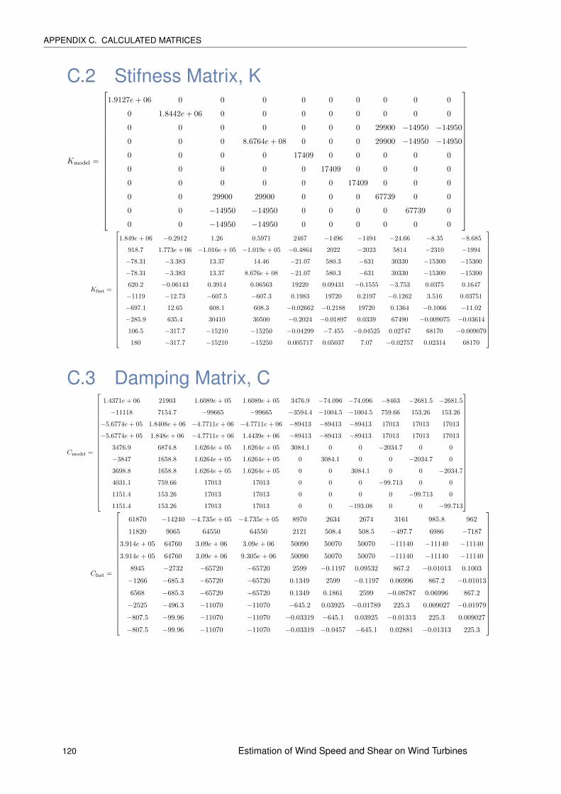
D Simulation and Linearisation by usage of FAST 121

iv Estimation of Wind Speed and Shear on Wind Turbines

CONTENTS

Estimation of Wind Speed and Shear on Wind Turbines 1

CONTENTS

NomenclatureR Radial distance from blade tip to rotor axis

r Radial distance from point on blade to rotor axis

H Height from ground surface to the wind turbine hub

z Height from ground surface to point on tower

β(t) Blade pitch angle

q Generalised coordinates

q Generalised velocities

q Generalised Accelerations

q1 Tower fore-aft displacement

q2 Tower side-side displacement

q3 Rotor azimuth angle

q4 Angle of drivetrain torsion

q5 Flapwise displacement of blade 1



q8 Edgewise displacement of blade 1



θk Azimuthal angle of kth blade

T (t, q, q) Total kinetic energy of the system

Tt(t, q) Kinetic energy of the tower

Tdt(t, q) Kinetic energy of the drivetrain

Tb(t, q, q) Kinetic energy of the blades

V (t, q) Total potential energy of the system

Vt(t, q) Potential energy of the tower

Vdt(t, q) Potential energy of the drivetrain

Vb(t, q) Potential energy of the blades

Q Generalised external forces

M Mass matrice

K Stiffness matrice

Ks Structural stiffness

Kg Gravity induced stiffness

Kc Centrifugal induced stiffness

2 Estimation of Wind Speed and Shear on Wind Turbines

CONTENTS

C Damping matrice

Cg Damping contributions from gyroscopical loads

Ca Aerodynamic damping

ζ Damping factor

Fak(t, r, vxk, vyk) Aerodynamic force on kth blade at radius r

FNk(t, r, vxk) Force component normal to plane of rotation at radius r

FTk(t, r, vyk) Force component tangential to plane of rotation at radius r

vxk(t, r) Relative wind along x-axis at radius r

vyk(t, r) Relative wind along y-axis at radius r

xbk(t, r) 1st coordinate of kth blade at radius r

ybk(t, r) 2nd coordinate of kth blade at radius r

fyk(r, θ) Effect of gravity on the kth blade at radius r and angle θ

Mn Mass of nacelle and rotor

µtfa(z) 1st mode shape of tower fore-aft displacement

µtss(z) 1st mode shape of tower side-side displacement

mt(z) Mass distribution of tower in height z

mb(r) Mass distribution of blade at r

EItfa(z) flexural rigidity in tower fore-aft direction at height z

EItss(z) flexural rigidity in tower side-side direction at height z

EIbf(r) flexural rigidity in blade flapwise direction at radius r

EIbe(r) flexural rigidity in blade edgewise direction at radius r

δtfa Slope of the mode shape µtfa at height H

δtss Slope of the mode shape µtss at height H

θt Torsional displacement of low speed shaft

θr Absolute angular position of rotor

θg Absolute angular position of generator

θgls Angular position of rotor on low speed side

n Gear ratio of drivetrain gear box

Jr Moment of inertia of the rotor

Jg Moment of inertia of the generator

τaero(t) Aerodynamic torque induced by wind

τl(t) Torque on gearbox at low speed side

τh(t) Torque on gearbox at high speed side

τg(t) Generator Torque

Bt Viscous damping of low speed shaft

Kt Stiffness of low speed shaft


CONTENTS

ϕ(r) Structural twist of blade at radius r

µbf(r) Flapwise mode shape of blade

µbe(r) Edgewise mode shape of blade

µbfop(r) Flapwise out-of-plane blade mode shape

µbfip(r) Flapwise in-plane blade mode shape

µbeop(r) Edgewise out-of-plane blade mode shape

µbeip(r) Edgewise in-plane mode blade shape

φ(r) Wind inflow angle at radius r

vk(r) Wind normal to the plane of rotation on kth blade

Wk(t, r, vxk, vyk) Relative wind on the kth blade

Ω Rotor speed

α(vk) Angle of attack

FLk(t, r, vxk, vyk) Lift force on the kth blade at radius r

FDk(t, r, vxk, vyk) Drag force on the kth blade at radius r

CL(r) Lift coefficient at radius r

CD(r) Drag coefficient at radius r

c(r) Chord length of blade cross section at radius r

FNk(t, r, vxk, vyk) Force normal to y-axis

FTk(t, r, vxk, vyk) Thrust force

FNvxk(r) Derivative of FN w.r.t. vxk

FNvyk(r) Derivative of FN w.r.t. vyk

FTvxk(r) Derivative of FT w.r.t. vxk

FTvxk(r) Derivative of FT w.r.t. vyk

vH(t) Mean wind in hub height (H)

vwsk(t) Wind shear wind component

vtsk(t) Tower shadow wind component


1 IntroductionOne of the most discussed issues in the world today, is the increasing need for renewableenergy sources. This is mainly because the fossil fuel sources are depleting, and because therequirements on CO2 emissions tightens. One of the renewable energy sources is the windturbine. For the wind turbine to replace today’s coal- and oil power plants, the designs ofthe wind turbines have over the last decade of years undergone a significant developmentin order to exploit the wind energy optimally[1]. To make the individual turbines moreefficient, the size of the wind turbines has increased, giving a greater wingspan, hence morewind energy can be exploited. However a greater wingspan leads to greater variations inthe wind characteristics over the swept area. Furthermore, the flexibility of the turbineshas as well increased as a trade-off from a light-weight design[1]. If the wind characteristicsare not taken properly into account when designing a wind turbine controller it can causean asymmetrical structural load on the blades and tower causing vibration and therebythe turbine to suffer unnecessary fatigue[1].

The most commonly used method for determining wind parameters is by usage of awind vane and an anemometer placed on the top of the nacelle. From these two sensorsmeasurements, an average wind speed and direction is calculated. The average windspeed is often either considered uniformly distributed across the entire disc shaped areaswept by the blades[2], or used as a parameter in a wind model describing how the windspeed changes vertically and horizontally. The wind measurements from the anemometerare nowadays only used for the purpose of shutting the turbine down, if higher windsare detected, than the turbine is rated for. However, they are thought to be useful foroptimizing wind energy production and minimise structural loading on the wind turbineif measured or estimated precise enough. The significance of the parameters increases asthe size of the wind turbine increases. Therefore, the importance of the accuracy of theestimated parameters rises as well in order to provide optimal control inputs.

The speed of the wind rises as a function of the height above ground surface[3]. Thisdifference is called the vertical wind shear. Furthermore the wind speed and direction isaffected by turbulence stochastically occurring in any point of the rotor swept area. Thegreater the wingspan, the more fluctuations and variation of the wind field is experiencedacross the span, which results in an asymmetrical aerodynamic loading. Estimating thewind field based on the measurements from wind vane and anemometer is thereforeinsufficient due to the fact that it is an average measurement and generally not veryinformative in terms of estimating useful wind field characteristics describing how thewind changes across the whole rotor swept area[4][5].

Therefore it is desirable to explore alternative sensors for obtaining measurements.An alternative way of estimating the wind field could be by usage of sensors mountedin the blades and tower. This could be done by e.g. strain gauges measuring

5

CHAPTER 1. INTRODUCTION

the stretching/bending of the element, or by accelerometer measuring the differentaccelerations of the element on which it is mounted. Based on the information aboutthe different elements on which the sensors are mounted the characteristics of the windfield could be determined.

From the statements above, the problem to be considered in this project is stated:

“How can wind shear and wind speed be estimated using measurement datafrom sensors mounted in the blades and tower of a wind turbine?”

1.1 Project OutlineAs mentioned in the preface, this report is divided into chapters containing sections andsubsections. This project outline is meant to give a more thorough overview on thestructure of the report.

Chapter 2: Wind Turbine SystemsThe purpose of this chapter is give an overview on the basics of how wind turbines arestructured and functions. Furthermore, the different characteristics of wind fields andtheir effect on the wind turbines are described. The chapter finishes by a description onwhich actuators are used to control modern wind turbines, and how they are controlled.

Chapter 3: Problem DescriptionThis chapter gives an overview of the sensors commonly used on modern wind turbinesfor determining wind fields. The chapter focuses on the drawbacks of these methodsregarding optimizing power production while minimising structural loadings and finaliseswith a discussion on proposals for control strategies for reduction of asymmetric loadingson the turbines.

Chapter 4: Requirement SpecificationThis chapter specifies the estimation problem, and states the wanted outcome of thisproject. It outlines the specific requirements that are set by the project group for thisproject to answer the problem statement.

Chapter 5: Acceptance Test DescriptionThis chapter specifies the tests needed to be carried out in order to determine whetherthe requirements specified in the requirement specification are met or not.

Chapter 6: Design OverviewThis chapter defines the design strategy chosen regarding model and estimation schemefor this project.


1.1. PROJECT OUTLINE

Chapter 7: Modelling a Wind TurbineThis chapter puts focus on how the wind turbine is modelled in this work. The turbineis divided into smaller subsystems: drivetrain, tower and blades which are modelledindividually. The aerodynamics are modelled and included to describe the interaction ofthis on the blades. The chosen wind model, containing the parameters wanted estimated,is presented. The chapter is concluded with some calculation examples on some of theentries for the system matrices describing the model.

Chapter 8: Estimating WindThis chapter describes the design of the wind -speed and -direction estimation scheme forthis project. First the different sensors considered applicable for the purpose are presentedalongside with their pros and cons. The assumed sensor setup is following described. Thechapter is concluded with a presentation of estimation strategies and the one used for thisproject is chosen.

Chapter 9: Implementation OverviewThis chapter picks up from previous chapter, and covers the description of theimplementation of the estimation scheme on the derived model.

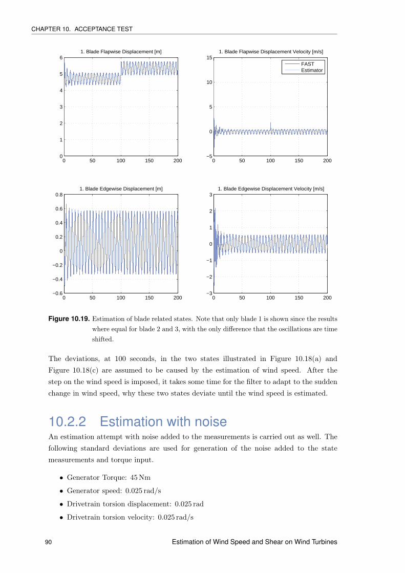
Chapter 10: Acceptance TestThis chapter covers the description of how it is tested whether the work made in thisproject answers the problem statement and fulfils the requirement specification. First adescription of the individual tests, followed by the results from the test and a discussion onthese. First the model is validated by simulations against the NREL 5 MW turbine fromthe FAST toolbox in MATLAB. Afterwards, the estimation scheme is tested on the model forits capability of estimating vertical wind shear and wind speed.

Chapter 11: ConclusionThis chapter concludes whether the approach done in this work for estimating wind -shear and -direction is profitable regarding optimisation of power production and/or theasymmetrical loadings on the wind turbine

Chapter 12: PerspectivesThis chapter describes further work that could be made on this project, assumed toimprove the results obtained. Also ideas for further inclusions in the derived model arediscussed.


Part I

Preliminary Analysis

9

2 Wind Turbine SystemThis chapter has the purpose of giving an overview of the structure and functionality of awind turbines. First the wind turbines physical and mechanical construction is describedto give an overview of the functionality. Afterwards the characteristics of a wind field andits effect on the wind turbine is described. Finally the means of controlling a wind turbineand the sensors used for control inputs are described.

2.1 Wind Turbines in GeneralA wind turbine is basically a construction, which converts the kinetic energy from thewind into electrical energy. The wind is caught by blades which makes the rotor rotate.The rotor is connected via a drivetrain to the generator which generates the electricalenergy.

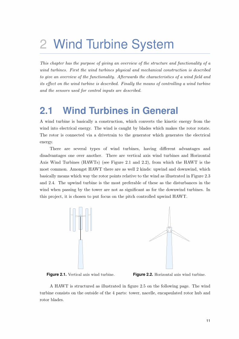
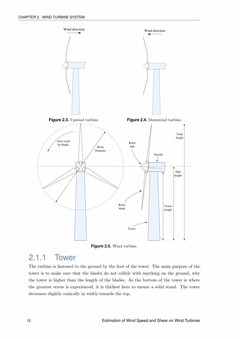
There are several types of wind turbines, having different advantages anddisadvantages one over another. There are vertical axis wind turbines and HorizontalAxis Wind Turbines (HAWTs) (see Figure 2.1 and 2.2), from which the HAWT is themost common. Amongst HAWT there are as well 2 kinds: upwind and downwind, whichbasically means which way the rotor points relative to the wind as illustrated in Figure 2.3and 2.4. The upwind turbine is the most preferable of these as the disturbances in thewind when passing by the tower are not as significant as for the downwind turbines. Inthis project, it is chosen to put focus on the pitch controlled upwind HAWT.

Figure 2.1. Vertical axis wind turbine. Figure 2.2. Horizontal axis wind turbine.

A HAWT is structured as illustrated in figure 2.5 on the following page. The windturbine consists on the outside of the 4 parts: tower, nacelle, encapsulated rotor hub androtor blades.

11

CHAPTER 2. WIND TURBINE SYSTEM

Wind direction

Figure 2.3. Upwind turbine.

Wind direction

Figure 2.4. Downwind turbine.

Area sweptby blades

RotorDiameter

Towerheight

Hubheight

Totalheight

Nacelle

Tower

Rotorhub

Rotorblade

Figure 2.5. Wind turbine.

2.1.1 TowerThe turbine is fastened to the ground by the foot of the tower. The main purpose of thetower is to make sure that the blades do not collide with anything on the ground, whythe tower is higher than the length of the blades. As the bottom of the tower is wherethe greatest stress is experienced, it is thickest here to ensure a solid stand. The towerdecreases slightly conically in width towards the top.


2.1. WIND TURBINES IN GENERAL

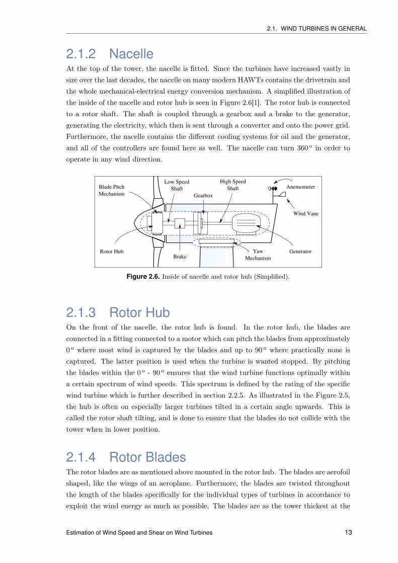
2.1.2 NacelleAt the top of the tower, the nacelle is fitted. Since the turbines have increased vastly insize over the last decades, the nacelle on many modern HAWTs contains the drivetrain andthe whole mechanical-electrical energy conversion mechanism. A simplified illustration ofthe inside of the nacelle and rotor hub is seen in Figure 2.6[1]. The rotor hub is connectedto a rotor shaft. The shaft is coupled through a gearbox and a brake to the generator,generating the electricity, which then is sent through a converter and onto the power grid.Furthermore, the nacelle contains the different cooling systems for oil and the generator,and all of the controllers are found here as well. The nacelle can turn 360 o in order tooperate in any wind direction.

Blade PitchMechanism

Rotor HubBrake

Gearbox

Low SpeedShaft

High SpeedShaft

YawMechanism

Generator

Anemometer

Wind Vane

Figure 2.6. Inside of nacelle and rotor hub (Simplified).

2.1.3 Rotor HubOn the front of the nacelle, the rotor hub is found. In the rotor hub, the blades areconnected in a fitting connected to a motor which can pitch the blades from approximately0 o where most wind is captured by the blades and up to 90 o where practically none iscaptured. The latter position is used when the turbine is wanted stopped. By pitchingthe blades within the 0 o - 90 o ensures that the wind turbine functions optimally withina certain spectrum of wind speeds. This spectrum is defined by the rating of the specificwind turbine which is further described in section 2.2.5. As illustrated in the Figure 2.5,the hub is often on especially larger turbines tilted in a certain angle upwards. This iscalled the rotor shaft tilting, and is done to ensure that the blades do not collide with thetower when in lower position.

2.1.4 Rotor BladesThe rotor blades are as mentioned above mounted in the rotor hub. The blades are aerofoilshaped, like the wings of an aeroplane. Furthermore, the blades are twisted throughoutthe length of the blades specifically for the individual types of turbines in accordance toexploit the wind energy as much as possible. The blades are as the tower thickest at the



bottom closest to the rotor hub, as this is where the greatest stress is seen. The bladesare often, on especially larger wind turbines, preconed which means that they are tiltedslightly upwind to ensure that they do not collide with the tower when operating in highwind speeds.

The different mechanical parts of the wind turbine, which are to be modelled in this project,have been described with the naming conventions used throughout the rest of the report.

2.2 Wind as Energy SourceThe behaviour of wind in general in an area is mainly dependent on the climate and thetopography in the given area. The wind field experienced by a wind turbine is thereforevariable in both time and space, affected by different parameters also including the windturbine itself[3]. It is relevant for wind turbine designs to have information on the winddirection and the wind speed across the rotor swept area in order to account for these, whentrying to maximise energy capture and minimise structural loading. In order to describethese changes across the rotor swept area, the wind field characteristics are described byseveral factors. The differences in wind speed and direction over the swept area are mainlycaused by the factors: wind shear, turbulence, tower shadow, and wake, which are brieflydescribed in the following.

2.2.1 Wind ShearWind shear refers to the change in wind speed over an area and occurs in three dimensionswhere horizontally and vertically shear are most relevant for wind turbines. Vertical shearis the most dominant shear effect on a wind turbine due to the ground slowing down thewind leading to the fact that the wind speed increases as a function of the height. Theeffect of shear is often described by using a mean wind speed which changes with theelevation above the ground. The mean wind speed and shear is typically considered as alow frequent variation which depends on the time of the day and the topography in thesurrounding area and is to some extend predictable[3, p. 7]. The vertical wind shear canbe modelled in several ways and in different variety of detail depending on the topographyin the area. The model used in this project is described in chapter 7 section 7.6.3.

2.2.2 TurbulenceThe effect of turbulence refers to changes in wind speed which occurs stochastically inperiods of minutes and down to seconds[1, p. 10]. The effect of turbulence has a minoreffect on the overall energy capture obtained by the wind turbine, whereas the low frequentvariations in the wind are more relevant. However the blades are affected by the stochasticchanges in the wind speed, which if the wind turbine is yawwise misaligned relative to the


2.2. WIND AS ENERGY SOURCE

wind direction causes asymmetrical loadings on the blades. These loadings propagatesfrom the blades to the drivetrain and tower. The quality of the power from the wind isalso affected by turbulence, since it can cause fluctuations in the angular velocity of therotor and thereby on the generator resulting in fluctuations in the power extracted, whichis not preferable when the turbine is connected to the electrical power grid.

2.2.3 Tower ShadowTower shadow occurs due to the presence of the tower blocking the wind, which needs toflow around the tower. This causes a drop in the wind speed, which leads to differencein aerodynamic loading on the blades when they move past the tower.[1, p. 219][3, p. 25].As well as for the wind shear, the tower shadow can be modelled in several ways. Themodel used in this project is described furtherer in chapter 7 section 7.6.4

2.2.4 WakeThe effect of wake refers to the fact that the wind speed and direction respectivelydecreases and changes as the wind passes through the rotor swept area. This is dueto the blades extracting kinetic energy from the wind, causing the rotor to rotate andresults in a drop in wind speed in the area on the backside of the rotor swept area. Thewake induced changes in wind direction occurs since the rotating blades has an impacton the wind field. The effect of wake is most relevant when considering wind farms wherethe wake effect of one turbine could affect neighbouring wind turbines[1, p. 33].

2.2.5 Power ExtractionThe theoretically maximum available energy from the wind can according to [6] bedescribed by

P =1

2mV 2

0

=1

2ρAV 3

0 (2.1)

where

P is the available energy [W]

m is the mass flow rate [kg/s]

V0 is the wind speed [m/s]

ρ is the density of the air[kg/m3

]A is the rotor swept area

[m2]

However, this is only theoretically and requires the wind speed to be fully reduced to zero,meaning that in the case of a wind turbine, the wind speed should be 0 after passingthrough the blades span in order to obtain the amount of energy that the formula 2.1



states. As this is not practically possible, a coefficient Cp is used to scale to find theactual power obtained. This coefficient has an upper limit called the Betz limit, CPmax

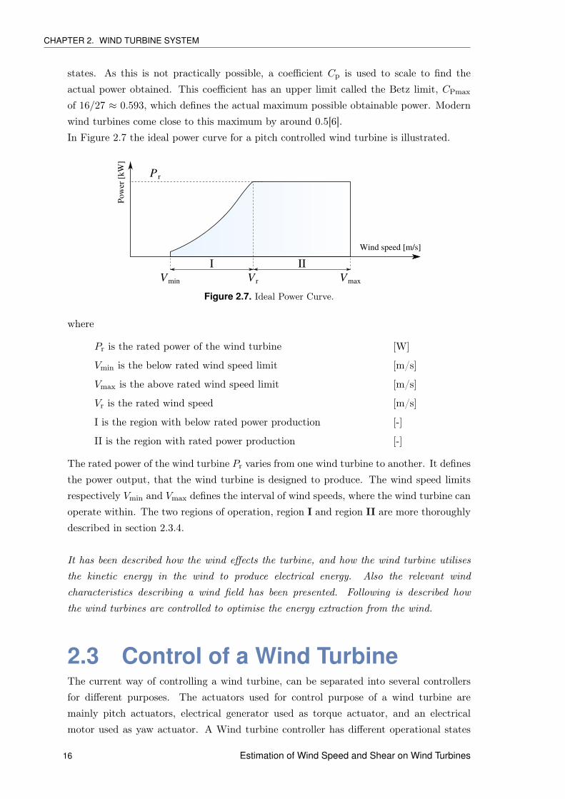
of 16/27 ≈ 0.593, which defines the actual maximum possible obtainable power. Modernwind turbines come close to this maximum by around 0.5[6].In Figure 2.7 the ideal power curve for a pitch controlled wind turbine is illustrated.

Vmin Vmax

P r

Pow

er [k

W]

Wind speed [m/s]

V r

I II

Figure 2.7. Ideal Power Curve.

where

Pr is the rated power of the wind turbine [W]

Vmin is the below rated wind speed limit [m/s]

Vmax is the above rated wind speed limit [m/s]

Vr is the rated wind speed [m/s]

I is the region with below rated power production [-]

II is the region with rated power production [-]

The rated power of the wind turbine Pr varies from one wind turbine to another. It definesthe power output, that the wind turbine is designed to produce. The wind speed limitsrespectively Vmin and Vmax defines the interval of wind speeds, where the wind turbine canoperate within. The two regions of operation, region I and region II are more thoroughlydescribed in section 2.3.4.

It has been described how the wind effects the turbine, and how the wind turbine utilisesthe kinetic energy in the wind to produce electrical energy. Also the relevant windcharacteristics describing a wind field has been presented. Following is described howthe wind turbines are controlled to optimise the energy extraction from the wind.

2.3 Control of a Wind TurbineThe current way of controlling a wind turbine, can be separated into several controllersfor different purposes. The actuators used for control purpose of a wind turbine aremainly pitch actuators, electrical generator used as torque actuator, and an electricalmotor used as yaw actuator. A Wind turbine controller has different operational states


2.3. CONTROL OF A WIND TURBINE

including, amongst others, standby, start-up, power production, shut-down or stoppeddue to failure. The active state is dependent on the turbine type and wind condition.In this project the only operational state considered is “power production”, why pitch-,torque- and yaw actuator are the only relevant actuators.

The inputs for the controller, in terms of measurements from different sensorsinstalled in the wind turbine, could be anemometer, wind vane, rotor speed sensor,electrical power sensor, pitch position sensors, accelerometers and load sensors wherethe latter two are placed in the blades, tower and the drivetrain. Based on these sensorinputs, outputs for the mentioned actuators can be calculated by a control algorithm. Therelevant actuators are described in the following.[1]

2.3.1 Pitch ActuatorThe pitch control is used to control how much power is generated from the aerodynamicload caused by the wind. When the wind speed is below the rated speed for a turbine,the turbine should extract as much power as possible from the wind, why there is no needfor pitching the blades. However for above rated wind speed, pitch control can be usedto vary the power extracted from the aerodynamic loading. Pitching of the blades can bedone either by using an individual or collective blade pitch approach.[3]

2.3.2 Torque ActuatorThe torque control is done in different ways dependent on whether variable- or fixed-speed operation is wanted. The type of generator used in both operation modes is anasynchronous induction generator. The torque developed in such a generator is developedas a result of slip speed between the rotor and the stator. When the rotor runs slower thanthe stator the generator acts as a motor and the slip is positive, for generator operationthe rotor runs faster than the stator and a negative slip is obtained giving a power output.

In a fixed-speed wind turbine the generator is connected to the electrical grid.Dependent on the grid frequency and number of magnetic poles in the generator asynchronous speed will be obtained. As the wind field varies the torque supplied bythe rotor will vary accordingly and thereby the generator torque will change to match thetorque supplied by the rotor, meaning the torque is not directly controllable.

In a variable-speed wind turbine different modifications can be done in order to obtainthe possibility of adjusting the generator speed. As an example a frequency converter isused to change the frequency experienced by the generator, making it possible to changethe synchronous generator speed[1].



2.3.3 Yaw ActuatorThe yaw control is used in order to point the wind turbine directly into the wind. This isdone in order to maximise the power output and to avoid asymmetric structural loadingon the wind turbine. An electric motor is used as actuator to turn the nacelle such thatit points into the wind. This is usually done based on sensor measurement from the windvane. The wind vane is for upwind turbines mounted on the top of the nacelle and istherefore subject to disturbances from the rotor. The measurements from the wind vaneis therefore averaged and if yaw misalignment reaches a certain level the yaw motor isused to correct for the error.[1].

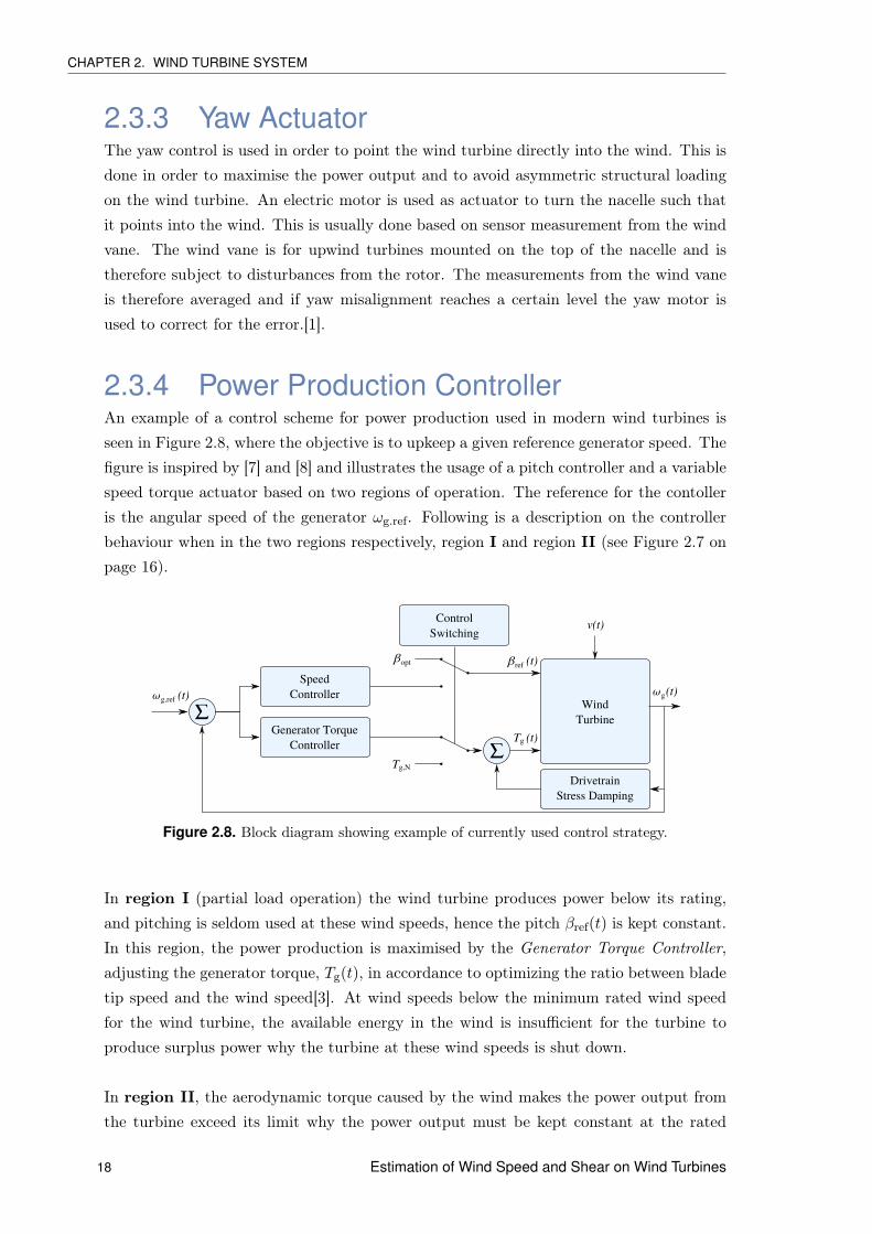
2.3.4 Power Production ControllerAn example of a control scheme for power production used in modern wind turbines isseen in Figure 2.8, where the objective is to upkeep a given reference generator speed. Thefigure is inspired by [7] and [8] and illustrates the usage of a pitch controller and a variablespeed torque actuator based on two regions of operation. The reference for the contolleris the angular speed of the generator ωg.ref. Following is a description on the controllerbehaviour when in the two regions respectively, region I and region II (see Figure 2.7 onpage 16).

Generator TorqueController

SpeedController

WindTurbine

DrivetrainStress Damping

ControlSwitching

Σ

Σ

βopt

ω (t)g,ref

Tg,N

v(t)

ω (t)g

β (t)ref

T (t)g

Figure 2.8. Block diagram showing example of currently used control strategy.

In region I (partial load operation) the wind turbine produces power below its rating,and pitching is seldom used at these wind speeds, hence the pitch βref(t) is kept constant.In this region, the power production is maximised by the Generator Torque Controller,adjusting the generator torque, Tg(t), in accordance to optimizing the ratio between bladetip speed and the wind speed[3]. At wind speeds below the minimum rated wind speedfor the wind turbine, the available energy in the wind is insufficient for the turbine toproduce surplus power why the turbine at these wind speeds is shut down.

In region II, the aerodynamic torque caused by the wind makes the power output fromthe turbine exceed its limit why the power output must be kept constant at the rated


2.3. CONTROL OF A WIND TURBINE

power. This constant output is kept by using the Speed Controller to control the pitchangle of the blades. The higher wind speeds, the greater pitch angle. At wind speedsabove the maximum rated wind speed for the wind turbine, the blades can be pitched nofurther and the wind turbine is shut down, as operation in this area could cause structuraloverload on the turbine[3].

The drivetrain stress damper is active at all time and has the purpose of limiting torqueoscillations in the gearbox. This is usually done by adding a rippled signal to the torqueinput, where the ripple frequency should be at the frequency of the torque oscillations.[8]

In this chapter, the structure and functions of modern wind turbines have been described.Also the characteristics of a wind field have been outlined, and the relevance of knowingthese from a control point of view.


3 Problem DescriptionThis chapter provides an overview of the currently typical usage of wind sensors forestimating the wind field on wind turbines, and which drawbacks it causes in termsof optimising the power production and minimising the loadings on tower, blades anddrivetrain. Afterwards the possibility of using alternative sensors to estimate wind fieldparameters is discussed, followed by a description on possible usages of it in a controller,which reduces the before mentioned asymmetrical loadings by usage of individual pitchcontrol.

Variations in the the wind field occur, as mentioned in chapter 2.2 on page 14, due to theeffect of wind shear, turbulence, tower shadow, and wake. The increase in size of the windturbines means that the area swept by the rotor blades becomes larger; hence the changesin the wind field become more significant as well, causing asymmetrical loading on thewind turbine. Therefore a detailed wind field estimation for preparation of a controllercompensating for asymmetrical aerodynamic loading would be beneficial.

3.1 SensorsThe most commonly used sensors in modern wind turbines to determine characteristics ofthe wind field, are a wind vane and an anemometer mounted on the top of the nacelle[3]as shown in Figure 2.6 on page 13. These sensors are used to determine an average windspeed and average wind direction. The sensors are affected by the wake of the windturbine which can cause noisy and unreliable measurements and thereby cause errors inthe determined wind speed and direction. Furthermore the sensors have dynamics interms of the inertia in the mechanical sensor construction which should be accounted forby modelling the dynamics of it, which can cause further errors in the measurement[9].

Since the wind direction is used as input on the yaw controller in order to point thewind turbine directly into the wind, an error in determining the wind direction will causeyaw misalignment. The effects of this is that the energy in the wind is not fully utilizedand an asymmetrical load on the blades and tower occurs. The wind speed measuredfrom the anemometer is only used to determine cut-in and cut-out speeds[4] for the windturbine, which are respectively the wind speeds at which the wind turbine is beneficialto turn on and the wind at which the turbine suffers overload; hence if the wind speedexceeds a certain level the wind turbine is shut down.

The quality and reliability of the wind speed and direction measurements makes itinsufficient for determination of the wind field experienced by the entire rotor, hence it isnot applicable for control purposes. Therefore additional sensors must be used if wanting

21

CHAPTER 3. PROBLEM DESCRIPTION

to estimate useful parameters of the wind. An approach could be to use sensors mountedin the blades and tower measuring loads and accelerations. In [1, p. 497] it is for instancesuggested to use load sensors in the blades. Another approach suggested by both Risøand National Renewable Energy Laboratory (NREL) is the usage of lidar placed in therotating hub, to detect the upwind inflow[10]. However a consequence of this method isthat the lidar makes use of the bending of a laser beam, which detects the wind speed ata certain distance ahead from the hub, which means that in case of turbulence, these datamight not be reliable to base a wind field estimation on[11, p. 7].

The usage of additional sensors could make it possible to obtain measurements ondeflection and vibrations caused by asymmetrical loading on the wind turbine structure.This asymmetrical loading could via modelling of wind disturbances be traced back toparameters used for control purpose.

In [5], it is attempted to calculate the effective wind speed, based on estimations ofrotor speed and aerodynamic torque by use of a combined state and input observer. In[12] it is suggested to use a set of strain gauges in combination with accelerometers, in acascade coupling of Kalman filters estimating wind field parameters, where a combinationof accelerometer and strain gauge yields deflection of blades and towers. In [5] the windspeed was calculated and [12]is still under development regarding estimation of the windfield parameters.

3.2 Reducing Asymmetric LoadingThe pitching of the blades is usually done collectively, meaning that the same pitch isapplied to all blades at once. The collective blade pitch results in the asymmetricalaerodynamic loading due to wind shear, tower shadow and turbulence not being takenproperly into account. This leads to increased structural fatigue and thereby shortens thelifetime of a wind turbine.

Therefore the possibility of using individual pitch control could be considered, sinceusage of such would make it possible to adjust the blade pitch based on the azimuthalangle of it. Measuring the load and vibration in the individual blades would make itpossible to predict the aerodynamic force experienced by a blade and accounting for it byusage of the individual pitch actuators.

The effect of vertical wind shear causes vibrations in the blades which propagatesto the tower, due to the blades experiencing different aerodynamic loading dependent ofangle position. The effect of shear is usually present and with very low frequent in changes,hence it can be considered constant and should be possible to detect and account for byindividual pitching.

Every time a blade passes the tower, tower shadow causes vibration in the bladesas well. It is therefore deterministic and could also be taken into account by usage ofindividual pitching.

Turbulence is stochastically occurring and therefore the asymmetrical loading caused


3.3. CONCLUSION

by it might not be possible to account for. The possibility of accounting for it dependson the length of the period in which the turbulence is occurring, and if any correlation isdetectable.

3.3 ConclusionThe possibility of compensating for the asymmetrical loading caused by the wind shouldbe possible by usage of azimuth dependent individual pitch control instead of collective.By considering the wind shear height dependent, and knowing that the tower shadowoccurs in a specific area of the rotor swept area, the pitching could be done cyclic. Inorder to implement a controller which pitches the blades individually additional sensorsalongside with wind field estimation should be used.


4 Requirement SpecificationThe previous chapter concluded that individual pitching, based on usage of anemometer andwind vane measurements, is insufficient due to the non-deterministic effect of turbulenceand errors in the measurements. This chapter will map out the requirements for anestimation of the wind field characteristics based on adding additional sensors to a windturbine.

4.1 The Estimation ProblemThe usage of anemometer and wind vane is insufficient for control purpose and thereforeusage of other sensors is required. Alternatively sensors used could be in terms ofaccelerometers and load sensors as e.g. strain gauges mounted in the tower and blades,which could yield information about deflection and vibrations presumably caused byasymmetrical loading from the wind field.

The main usage could be to utilise the possibility of using individual pitch control inorder to compensate for asymmetrical loading caused by difference in wind fields acrossthe wingspan. This project is confined to include only the effects of wind shear and windspeed for estimation, based on usage of load sensors and accelerometers. This means, thatthe model does not account for yaw error, turbulence and wake. Therefore the followingrequirements are set.

r.1 Derive a model describing blade and tower deflections and vibrationscaused by wind perturbation.

A model for usage in estimation of the wind field parameters must be designed in orderto see the effects of wind field characteristics on the blade and tower vibrations anddeflections.

r.2 Estimate wind parameters based on loading measurements.

An estimation scheme must be designed in order to determine wind field characteristicsin terms of vertical shear and wind speed.

25

5 Acceptance Test DescriptionThis chapter describes how the outlined requirement will be tested.

Requirement r.1 will be tested in the following way: The derived model will be adopted inMATLAB for validation. It is then chosen to use the NREL FAST toolbox[13], as a benchmarkfor the validation, since this software is known and acknowledged for its performance[13].The used turbine model will be the NREL 5 MW Onshore wind turbine[14]. Therequirement is met if the derived model’s response to control inputs and wind disturbancescorresponds to the output from FAST. This is e.g. assessed based on the eigen-frequenciesof the output.

Requirement r.2 will be tested in the following way: A simulation will be carried outin FAST where the wind field will be specified by given values for shear, wind speed andyaw error. The estimation scheme will then be tested by comparing the estimated windfield parameters to the ones specified in the wind simulation. The requirement will beconsidered met if there is agreement between the simulated and estimated wind fieldparameters.

27

Part II

Design andImplementation

29

6 Design OverviewThis chapter provides an overview on the design strategy for fulfilling the requirementsregarding the estimation problem described in chapter 4.

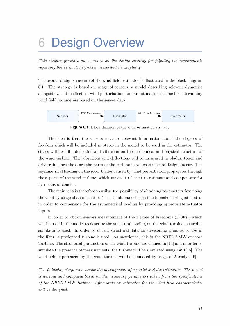
The overall design structure of the wind field estimator is illustrated in the block diagram6.1. The strategy is based on usage of sensors, a model describing relevant dynamicsalongside with the effects of wind perturbation, and an estimation scheme for determiningwind field parameters based on the sensor data.

EstimatorSensorsDOF Measurement Wind State Estimates

Controller

Figure 6.1. Block diagram of the wind estimation strategy.

The idea is that the sensors measure relevant information about the degrees offreedom which will be included as states in the model to be used in the estimator. Thestates will describe deflection and vibration on the mechanical and physical structure ofthe wind turbine. The vibrations and deflections will be measured in blades, tower anddrivetrain since these are the parts of the turbine in which structural fatigue occur. Theasymmetrical loading on the rotor blades caused by wind perturbation propagates throughthese parts of the wind turbine, which makes it relevant to estimate and compensate forby means of control.

The main idea is therefore to utilise the possibility of obtaining parameters describingthe wind by usage of an estimator. This should make it possible to make intelligent controlin order to compensate for the asymmetrical loading by providing appropriate actuatorinputs.

In order to obtain sensors measurement of the Degree of Freedoms (DOFs), whichwill be used in the model to describe the structural loading on the wind turbine, a turbinesimulator is used. In order to obtain structural data for developing a model to use inthe filter, a predefined turbine is used. As mentioned, this is the NREL 5 MW onshoreTurbine. The structural parameters of the wind turbine are defined in [14] and in order tosimulate the presence of measurements, the turbine will be simulated using FAST[15]. Thewind field experienced by the wind turbine will be simulated by usage of Aerodyn[16].

The following chapters describe the development of a model and the estimator. The modelis derived and computed based on the necessary parameters taken from the specificationsof the NREL 5 MW turbine. Afterwards an estimator for the wind field characteristicswill be designed.

31

7 Modelling a Wind TurbineThis chapter describes considerations and assumptions done with regard to modelling thewind turbine in this work. The turbine is divided in three mechanical subsystems, beingthe drivetrain, a flexible tower and flexible blades. Finally the aerodynamics is includedas a subsystem in the model to describe the interaction between the wind and the turbineblades.

The purpose of this chapter is to derive a non-linear model and an LPV model like the oneproposed in [7]. It is chosen to derive both types of models to allow for different estimationschemes to be tested. In this work, tower and blades are regarded as flexible structuresand therefore have distributed parameters, yielding them an infinite number of modes.However, this can not be implemented, and it is therefore assumed that the tower andblades only possess a finite, and low number of modes. This model simplification methodis known as the Assumed Modes Method[17]. Other alternatives such as Finite ElementMethod can be used to approximate a system with distributed parameters. However this iscomputational heavy[18], and is therefore not considered furtherer. In this work it is chosenonly to use the first mode shape of each of the flexible structures. This assumption is madeto keep the number of states in the filter low, in order to reduce computation. To simplifyderivations, the precone of the blades, the shaft tilt and the rotor overhang are neglected.These effects are however included in the wind turbine model of the simulation tool FAST,which the model of this work is intended to be validated against. Parameters such as modeshapes, mass distributions, flexural rigidity distributions, ect. are obtained from the FASTinput files for the NREL 5 MW wind turbine, which is used for the validation[15]. Thederivation procedure done in this work is done in accordance to the following steps:

• Obtain data from FAST.

• Approximate mass distribution, stiffness distribution, etc. from data.

• Apply Lagrangian Mechanics to derive generalised Mass, Stiffness and Damping.

• Generalise the aero-dynamical force.

• Include gravity load as additional stiffness.

33

CHAPTER 7. MODELLING A WIND TURBINE

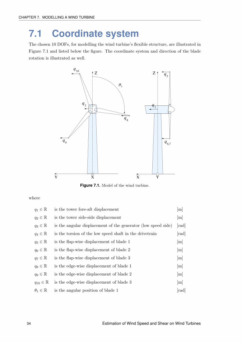
7.1 Coordinate systemThe chosen 10 DOFs, for modelling the wind turbine’s flexible structure, are illustrated inFigure 7.1 and listed below the figure. The coordinate system and direction of the bladerotation is illustrated as well.

XY

Z

q1

X Y

Z q5

q6,7

q8

q9

q10

q2

𝜃1

Figure 7.1. Model of the wind turbine.

where

q1 ∈ R is the tower fore-aft displacement [m]

q2 ∈ R is the tower side-side displacement [m]

q3 ∈ R is the angular displacement of the generator (low speed side) [rad]

q4 ∈ R is the torsion of the low speed shaft in the drivetrain [rad]

q5 ∈ R is the flap-wise displacement of blade 1 [m]



q8 ∈ R is the edge-wise displacement of blade 1 [m]



θ1 ∈ R is the angular position of blade 1 [rad]


7.2. MODELLING

7.2 ModellingTo derive a model that describes the dynamics of a wind turbine, Lagrangian mechanicsis used[19, p. 21].

Consider the Lagrangian

L(t, q, q) = T(t, q, q)− V(t, q), [J] (7.1)

where

q ∈ Rn are the generalised coordinates,

q ∈ Rn are the generalised velocities,

L ∈ R is the Lagrangian, [J]

T ∈ R is the kinetic energy of the system, [J]

V ∈ R is the potential energy of the system. [J]

The considered system has 10 DOFs i.e. n = 10. For the wind turbine, it should be notedthat the kinetic energy is not only a function of time and generalised coordinates, but alsothe generalised velocities. This is due to the rotation of the blades, which will introducegyroscopic and centrifugal loads. The kinetic and potential energy of the system are sumsof several energy contributions. These contributions are from the tower, the drivetrainand the blades. Hence, the kinetic energy is

T(t, q, q) = Tt(t, q) + Tdt(t, q) + Tb(t, q, q), [J] (7.2)

and the potential energy is

V(t, q) = Vt(t, q) + Vdt(t, q) + Vb(t, q), [J] (7.3)

The Euler-Lagrange equation for a system subject to external forces is

0 =d

dt

(∂L(t, q, q)

∂q

)− ∂L(t, q, q)

∂q+∂F(t, q)

∂q−Q(t), (7.4)

where

F ∈ R is Rayleigh’s dissipation function, [W]

Q ∈ Rn is the generalised, external forces.

In the considered system there are several external forces, interacting with the windturbine. They consist of both conservative and non-conservative forces. The externalforces are the following

Q = Qττ(t) +Qg +Qa (7.5)



where

Qτ ∈ R10 is the gain of the torque applied by the generator,

Qg ∈ R10 is the generalised force induced by gravity,

Qa ∈ R10 is the generalised force induced by the aerodynamics,

τ ∈ R is the applied generator torque.

The considered system is subject to two non-conservative forces, which are friction andaerodynamics. Both of these forces contribute to the damping of the system, which arerespectively denoted as structural- and aerodynamic damping. A third contribution tothe damping is caused by gyroscopic loading due to blade rotation, which is seen later ina derivation example.

The Euler-Lagrange equation (eq. 7.4) has four terms in this case. The first two relateto respectively mass and structural stiffness of the system. The third is the structuralfriction in the wind turbine. The generalised forces introduce the aerodynamic damping,a gravity induced stiffness[7] and the last term is considered a controlled input. A thirdterm contributing to the stiffness of the system arises from centrifugal loads on the blades.This stiffness term can not readily be seen from the Euler-Lagrange equation, but will bemore obvious from the derivation example presented in section 7.7 on page 56. Considerthe Euler-Lagrange equation and all the mentioned stiffness and damping terms, then thenon-linear system dynamics of the wind turbine has the following form

Qττ(t) +Qa(t) = Mq(t) + (Cs + Cg)q(t) + (Ks +Kg +Kc)q(t), (7.6)

where

q ∈ R10 is the generalised acceleration,

M ∈ R10×10 is the mass matrix,

Cs ∈ R10×10 is the structural damping,

Cg ∈ R10×10 is the damping due to gyroscopic loads,

Ks ∈ R10×10 is the structural stiffness,

Kg ∈ R10×10 is the stiffness induced by gravity,

Kc ∈ R10×10 is the stiffness due centrifugal loads.

The eq. 7.6 describes the wind turbine system. It is however non-linear due tothe aerodynamic forces Qa(t). The following subsection explains how to linearise theaerodynamics in order to obtain an LPV model.

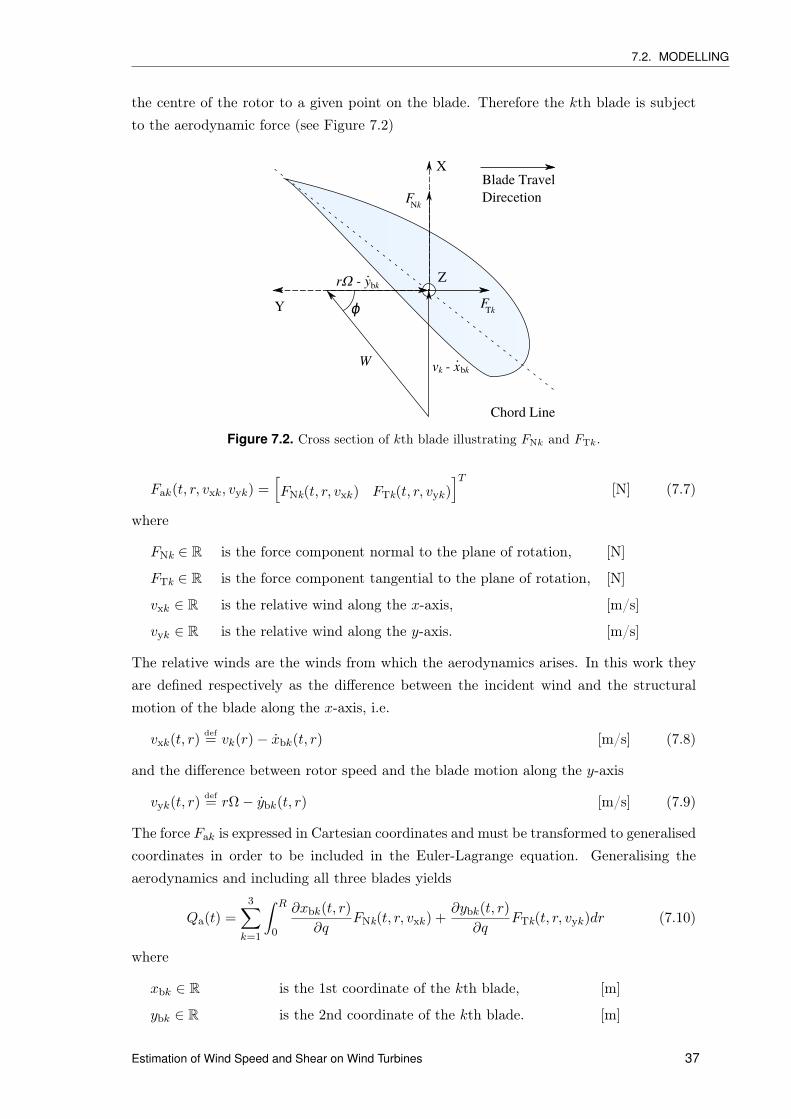
7.2.1 Generalised Aerodynamic ForceThe aerodynamic force arises from the interaction between the wind and each of the blades.This force depends on position of the blade, i.e. the radius r, which is the distance from


7.2. MODELLING

the centre of the rotor to a given point on the blade. Therefore the kth blade is subjectto the aerodynamic force (see Figure 7.2)

X

Y

Z

Chord Line

Blade TravelDirecetionFNk

FTk

v - xW

ϕ

rΩ - y.

.

bk

bkk

Figure 7.2. Cross section of kth blade illustrating FNk and FTk.

Fak(t, r, vxk, vyk) =[FNk(t, r, vxk) FTk(t, r, vyk)

]T[N] (7.7)

where

FNk ∈ R is the force component normal to the plane of rotation, [N]

FTk ∈ R is the force component tangential to the plane of rotation, [N]

vxk ∈ R is the relative wind along the x-axis, [m/s]

vyk ∈ R is the relative wind along the y-axis. [m/s]

The relative winds are the winds from which the aerodynamics arises. In this work theyare defined respectively as the difference between the incident wind and the structuralmotion of the blade along the x-axis, i.e.

vxk(t, r)def= vk(r)− xbk(t, r) [m/s] (7.8)

and the difference between rotor speed and the blade motion along the y-axis

vyk(t, r)def= rΩ− ybk(t, r) [m/s] (7.9)

The force Fak is expressed in Cartesian coordinates and must be transformed to generalisedcoordinates in order to be included in the Euler-Lagrange equation. Generalising theaerodynamics and including all three blades yields

Qa(t) =

3∑k=1

∫ R

0

∂xbk(t, r)

∂qFNk(t, r, vxk) +

∂ybk(t, r)

∂qFTk(t, r, vyk)dr (7.10)

where

xbk ∈ R is the 1st coordinate of the kth blade, [m]

ybk ∈ R is the 2nd coordinate of the kth blade. [m]



The aerodynamics is non-linear w.r.t. the generalised velocity q, the pitch control input βand the speed of the incident wind vk. Therefore the aerodynamic force is linearised w.r.t.each of those variables to derive the LPV model. The linearisation splits the generalisedaerodynamics into the three terms

Qa =∂Qa

∂qq(t) +

∂Qa

∂ββ(t) +

∂Qa

∂vkvk(t) (7.11)

Qa = Caq(t) +Qββ(t) +Qvvk(t) (7.12)

where

Qa ∈ R10 is the perturbations in the generalised force from its operating point,

Ca ∈ R10×10 is the aerodynamic damping,

Qβ ∈ R3×10 is the gain for perturbations of the pitch angle,

Qv ∈ R3×10 is the gain for perturbations of the incident wind’s speed.

The first term of Qa depends on the generalised velocity, q(t), and can therefore be treatedas additional damping in the system. This damping is referred to as aerodynamic damping.The two other terms depend respectively on input and disturbance and are thereforetreated as forcing functions of the system. The linearised system is

Qττ(t) +Qββ(t) +Qvvk(t) = Mq(t) + (Cs + Cg − Ca)q(t) + (Ks +Kg +Kc)q(t),

(7.13)

The system in equation 7.13 is linear, however still azimuth dependent, so the matricesmust be evaluated for each time step, when used for control or estimation. It is noticeablethat the aerodynamic damping matrix has a negative sign, however each entry of thematrix will also have negative sign. The aerodynamic therefore contribute with a positivedamping as expected.

The gains for the forcing vectors are found by combining eq. 7.10 and eq. 7.11, giving theaerodynamic damping as

cija =3∑

k=1

∫ R

0

∂xbk

∂qi

[∂FNk

∂vxk

∂vxk

∂qj+∂FNk

∂vyk

∂vyk

∂qj

]+∂ybk

∂qi

[∂FTk

∂vxk

∂vxk

∂qj+∂FTk

∂vyk

∂vyk

∂qj

]dr, (7.14)

and the gain coefficients of the pitch input are

Qβij =

3∑k=1

∫ R

0

∂xbk

∂qi

∂FNk

∂βj+∂ybk

∂qi

∂FTk

∂βjdr, (7.15)

and the gain coefficients of the incident wind disturbance are

Qvij =3∑

k=1

∫ R

0

∂xbk

∂qi

∂FNk

∂vj+∂ybk

∂qi

∂FTk

∂vjdr, (7.16)

This concludes the description of the aerodynamics. The other external forces in thissystem are explained in the following subsections. The force applied from the generatoris described in connection with drivetrain model.


7.2. MODELLING

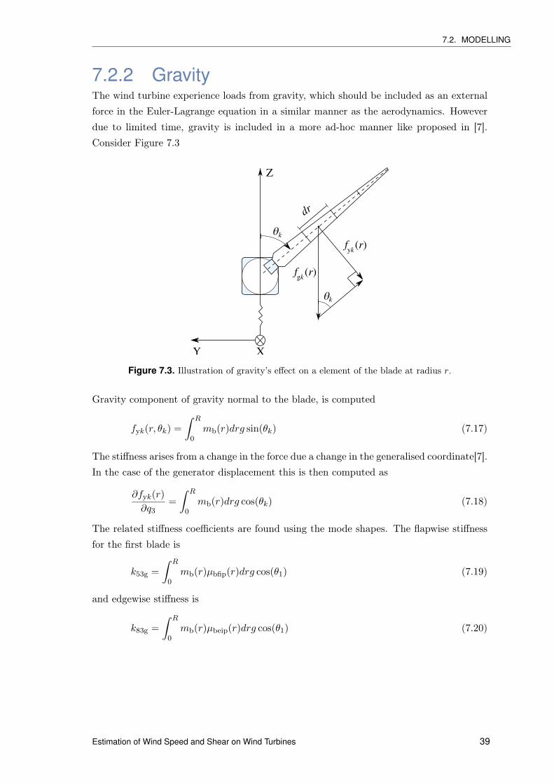
7.2.2 GravityThe wind turbine experience loads from gravity, which should be included as an externalforce in the Euler-Lagrange equation in a similar manner as the aerodynamics. Howeverdue to limited time, gravity is included in a more ad-hoc manner like proposed in [7].Consider Figure 7.3

XY

Z

𝜃

dr

𝜃

(r)fgk

(r)fyk

.k

k

Figure 7.3. Illustration of gravity’s effect on a element of the blade at radius r.

Gravity component of gravity normal to the blade, is computed

fyk(r, θk) =

∫ R

0mb(r)drg sin(θk) (7.17)

The stiffness arises from a change in the force due a change in the generalised coordinate[7].In the case of the generator displacement this is then computed as

∂fyk(r)

∂q3=

∫ R

0mb(r)drg cos(θk) (7.18)

The related stiffness coefficients are found using the mode shapes. The flapwise stiffnessfor the first blade is

k53g =

∫ R

0mb(r)µbfip(r)drg cos(θ1) (7.19)

and edgewise stiffness is

k83g =

∫ R

0mb(r)µbeip(r)drg cos(θ1) (7.20)



7.2.3 Structural DampingThe structural damping of the wind turbine is found by considering the non-conservativeforce of friction. The friction is included using Rayleigh’s dissipation function[19, p. 24]

F(t, q) =1

2q(t)TCsq(t). [W] (7.21)

Here Cs is a diagonal matrix, which contains the structural (viscous) damping coefficientsin the diagonal entries. These coefficients are given as

ciis = 2ζi√kiimii, [Ns/m] (7.22)

where

Cs ∈ R10×10 is the structural dampning,

ciis ∈ R is the iith structural damping coefficient,

ζi ∈ R is the ith damping factor. [-]

kii ∈ R is the iith stiffness coefficient.

mii ∈ R is the iith mass coefficient.

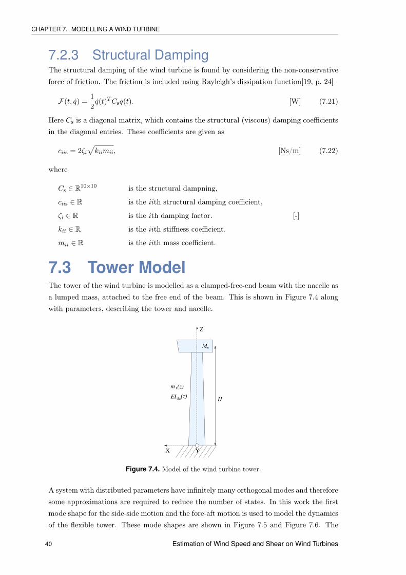
7.3 Tower ModelThe tower of the wind turbine is modelled as a clamped-free-end beam with the nacelle asa lumped mass, attached to the free end of the beam. This is shown in Figure 7.4 alongwith parameters, describing the tower and nacelle.

M

H

X Y

Z

m t(z)

EI tfa(z)

n

Figure 7.4. Model of the wind turbine tower.

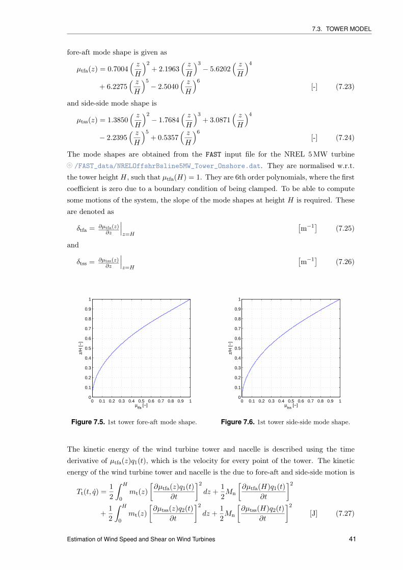
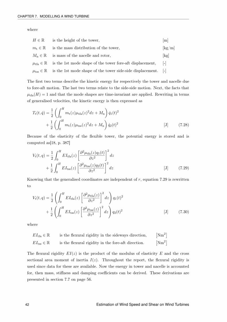
A system with distributed parameters have infinitely many orthogonal modes and thereforesome approximations are required to reduce the number of states. In this work the firstmode shape for the side-side motion and the fore-aft motion is used to model the dynamicsof the flexible tower. These mode shapes are shown in Figure 7.5 and Figure 7.6. The


7.3. TOWER MODEL

fore-aft mode shape is given as

µtfa(z) = 0.7004( zH

)2+ 2.1963

( zH

)3− 5.6202

( zH

)4

+ 6.2275( zH

)5− 2.5040

( zH

)6[-] (7.23)

and side-side mode shape is

µtss(z) = 1.3850( zH

)2− 1.7684

( zH

)3+ 3.0871

( zH

)4

− 2.2395( zH

)5+ 0.5357

( zH

)6[-] (7.24)

The mode shapes are obtained from the FAST input file for the NREL 5 MW turbine/FAST_data/NRELOffshrBsline5MW_Tower_Onshore.dat. They are normalised w.r.t.

the tower heightH, such that µtfa(H) = 1. They are 6th order polynomials, where the firstcoefficient is zero due to a boundary condition of being clamped. To be able to computesome motions of the system, the slope of the mode shapes at height H is required. Theseare denoted as

δtfa = ∂µtfa(z)∂z

∣∣∣z=H

[m−1

](7.25)

and

δtss = ∂µtss(z)∂z

∣∣∣z=H

[m−1

](7.26)

0 0.1 0.2 0.3 0.4 0.5 0.6 0.7 0.8 0.9 10

0.1

0.2

0.3

0.4

0.5

0.6

0.7

0.8

0.9

1

µtfa

[−]

z/H

[−]

Figure 7.5. 1st tower fore-aft mode shape.

0 0.1 0.2 0.3 0.4 0.5 0.6 0.7 0.8 0.9 10

0.1

0.2

0.3

0.4

0.5

0.6

0.7

0.8

0.9

1

µtss

[−]

z/H

[−]

Figure 7.6. 1st tower side-side mode shape.

The kinetic energy of the wind turbine tower and nacelle is described using the timederivative of µtfa(z)q1(t), which is the velocity for every point of the tower. The kineticenergy of the wind turbine tower and nacelle is the due to fore-aft and side-side motion is

Tt(t, q) =1

2

∫ H

0mt(z)

[∂µtfa(z)q1(t)

∂t

]2

dz +1

2Mn

[∂µtfa(H)q1(t)

∂t

]2

+1

2

∫ H

0mt(z)

[∂µtss(z)q2(t)

∂t

]2

dz +1

2Mn

[∂µtss(H)q2(t)

∂t

]2

[J] (7.27)



where

H ∈ R is the height of the tower, [m]

mt ∈ R is the mass distribution of the tower, [kg/m]

Mn ∈ R is mass of the nacelle and rotor, [kg]

µtfa ∈ R is the 1st mode shape of the tower fore-aft displacement, [-]

µtss ∈ R is the 1st mode shape of the tower side-side displacement. [-]

The first two terms describe the kinetic energy for respectively the tower and nacelle dueto fore-aft motion. The last two terms relate to the side-side motion. Next, the facts thatµtfa(H) = 1 and that the mode shapes are time-invariant are applied. Rewriting in termsof generalised velocities, the kinetic energy is then expressed as

Tt(t, q) =1

2

(∫ H

0mt(z)µtfa(z)2dz +Mn

)q1(t)2

+1

2

(∫ H

0mt(z)µtss(z)

2dz +Mn

)q2(t)2 [J] (7.28)

Because of the elasticity of the flexible tower, the potential energy is stored and iscomputed as[18, p. 387]

Vt(t, q) =1

2

∫ H

0EItfa(z)

[∂2µtfa(z)q1(t)

∂z2

]2

dz

+1

2

∫ H

0EItss(z)

[∂2µtss(z)q2(t)

∂z2

]2

dz [J] (7.29)

Knowing that the generalised coordinates are independent of r, equation 7.29 is rewrittento

Vt(t, q) =1

2

(∫ H

0EItfa(z)

[∂2µtfa(z)

∂z2

]2

dz

)q1(t)2

+1

2

(∫ H

0EItss(z)

[∂2µtss(z)

∂z2

]2

dz

)q2(t)2 [J] (7.30)

where

EItfa ∈ R is the flexural rigidity in the sideways direction,[Nm2

]EItss ∈ R is the flexural rigidity in the fore-aft direction.

[Nm2

]The flexural rigidity EI(z) is the product of the modulus of elasticity E and the crosssectional area moment of inertia I(z). Throughout the report, the flexural rigidity isused since data for these are available. Now the energy in tower and nacelle is accountedfor, then mass, stiffness and damping coefficients can be derived. These derivations arepresented in section 7.7 on page 56.


7.4. DRIVETRAIN MODEL

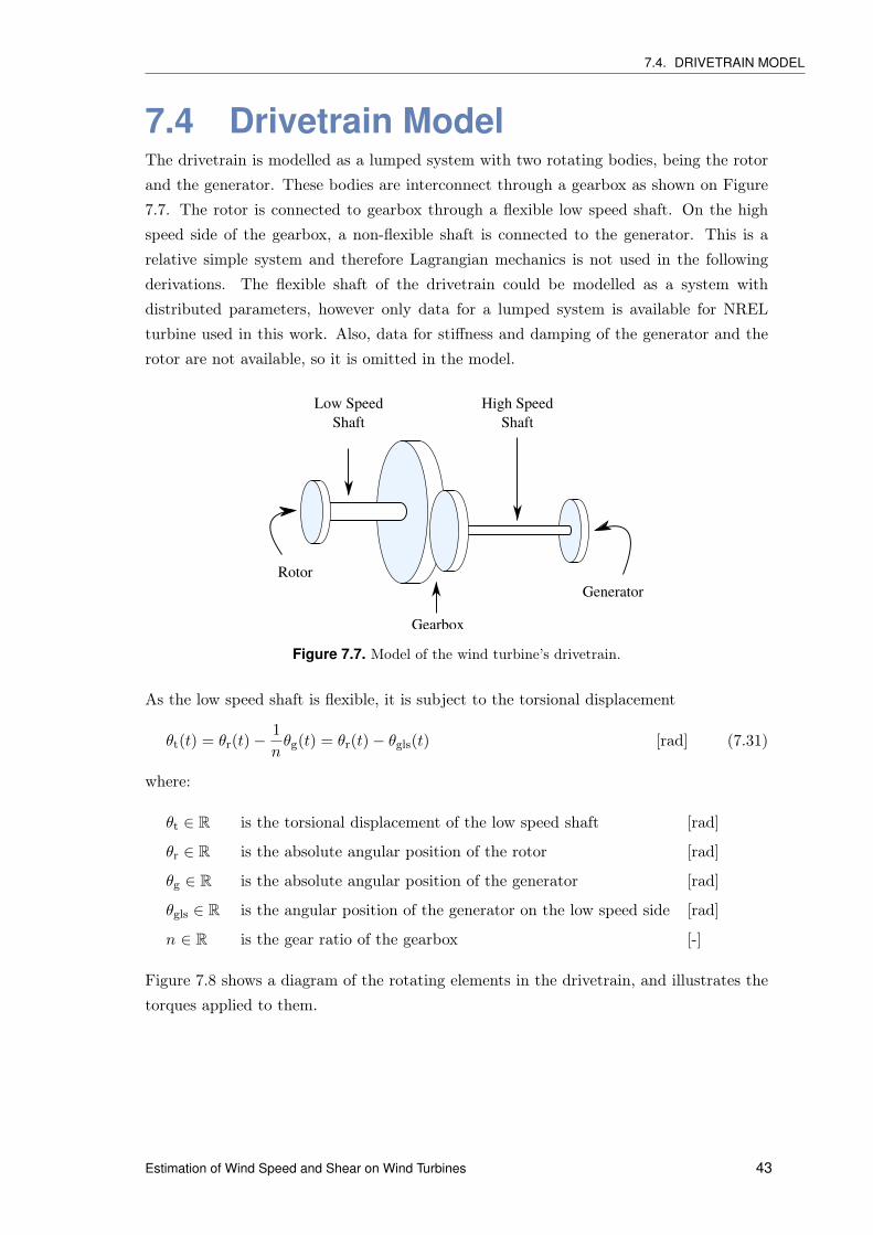
7.4 Drivetrain ModelThe drivetrain is modelled as a lumped system with two rotating bodies, being the rotorand the generator. These bodies are interconnect through a gearbox as shown on Figure7.7. The rotor is connected to gearbox through a flexible low speed shaft. On the highspeed side of the gearbox, a non-flexible shaft is connected to the generator. This is arelative simple system and therefore Lagrangian mechanics is not used in the followingderivations. The flexible shaft of the drivetrain could be modelled as a system withdistributed parameters, however only data for a lumped system is available for NRELturbine used in this work. Also, data for stiffness and damping of the generator and therotor are not available, so it is omitted in the model.

Low SpeedShaft

High SpeedShaft

Gearbox

GeneratorRotor

Figure 7.7. Model of the wind turbine’s drivetrain.

As the low speed shaft is flexible, it is subject to the torsional displacement

θt(t) = θr(t)−1

nθg(t) = θr(t)− θgls(t) [rad] (7.31)

where:

θt ∈ R is the torsional displacement of the low speed shaft [rad]

θr ∈ R is the absolute angular position of the rotor [rad]

θg ∈ R is the absolute angular position of the generator [rad]

θgls ∈ R is the angular position of the generator on the low speed side [rad]

n ∈ R is the gear ratio of the gearbox [-]

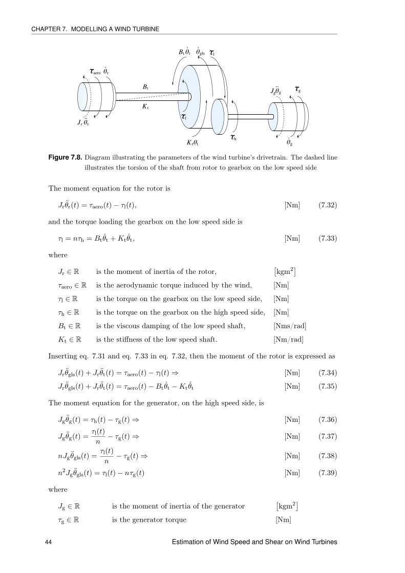
Figure 7.8 shows a diagram of the rotating elements in the drivetrain, and illustrates thetorques applied to them.



𝜃.

r

K t

Bt

τl

τaero

Jr 𝜃.

r.

Bt 𝜃.

t

K t𝜃t

𝜃.

gls τl

τh𝜃.

g

τg𝜃..

gJg

Figure 7.8. Diagram illustrating the parameters of the wind turbine’s drivetrain. The dashed lineillustrates the torsion of the shaft from rotor to gearbox on the low speed side

The moment equation for the rotor is

Jrθr(t) = τaero(t)− τl(t), [Nm] (7.32)

and the torque loading the gearbox on the low speed side is

τl = nτh = Btθt +Ktθt, [Nm] (7.33)

where

Jr ∈ R is the moment of inertia of the rotor,[kgm2

]τaero ∈ R is the aerodynamic torque induced by the wind, [Nm]

τl ∈ R is the torque on the gearbox on the low speed side, [Nm]

τh ∈ R is the torque on the gearbox on the high speed side, [Nm]

Bt ∈ R is the viscous damping of the low speed shaft, [Nms/rad]

Kt ∈ R is the stiffness of the low speed shaft. [Nm/rad]

Inserting eq. 7.31 and eq. 7.33 in eq. 7.32, then the moment of the rotor is expressed as

Jrθgls(t) + Jrθt(t) = τaero(t)− τl(t)⇒ [Nm] (7.34)

Jrθgls(t) + Jrθt(t) = τaero(t)−Btθt −Ktθt [Nm] (7.35)

The moment equation for the generator, on the high speed side, is

Jgθg(t) = τh(t)− τg(t)⇒ [Nm] (7.36)

Jgθg(t) =τl(t)

n− τg(t)⇒ [Nm] (7.37)

nJgθgls(t) =τl(t)

n− τg(t)⇒ [Nm] (7.38)

n2Jgθgls(t) = τl(t)− nτg(t) [Nm] (7.39)

where

Jg ∈ R is the moment of inertia of the generator[kgm2

]τg ∈ R is the generator torque [Nm]


7.5. BLADE MODEL

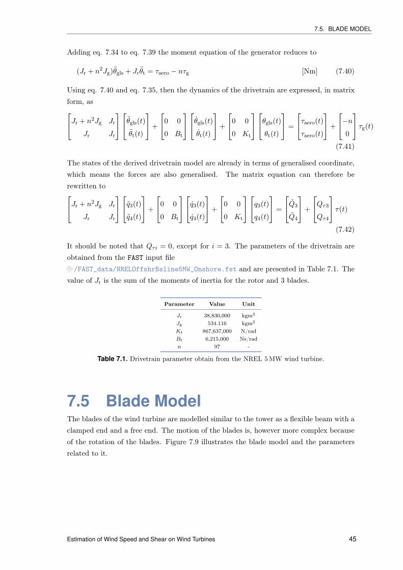
Adding eq. 7.34 to eq. 7.39 the moment equation of the generator reduces to

(Jr + n2Jg)θgls + Jrθt = τaero − nτg [Nm] (7.40)

Using eq. 7.40 and eq. 7.35, then the dynamics of the drivetrain are expressed, in matrixform, asJr + n2Jg Jr

Jr Jr

θgls(t)

θt(t)

+

0 0

0 Bt

θgls(t)

θt(t)

+

0 0

0 Kt

θgls(t)

θt(t)

=

τaero(t)

τaero(t)

+

−n0

τg(t)

(7.41)

The states of the derived drivetrain model are already in terms of generalised coordinate,which means the forces are also generalised. The matrix equation can therefore berewritten toJr + n2Jg Jr

Jr Jr

q3(t)

q4(t)

+

0 0

0 Bt

q3(t)

q4(t)

+

0 0

0 Kt

q3(t)

q4(t)

=

Q3

Q4

+

Qτ3

Qτ4

τ(t)

(7.42)

It should be noted that Qτi = 0, except for i = 3. The parameters of the drivetrain areobtained from the FAST input file/FAST_data/NRELOffshrBsline5MW_Onshore.fst and are presented in Table 7.1. The

value of Jr is the sum of the moments of inertia for the rotor and 3 blades.

Parameter Value Unit

Jr 38,830,000 kgm2

Jg 534.116 kgm2

Kt 867,637,000 N/radBt 6,215,000 Ns/radn 97 -

Table 7.1. Drivetrain parameter obtain from the NREL 5 MW wind turbine.

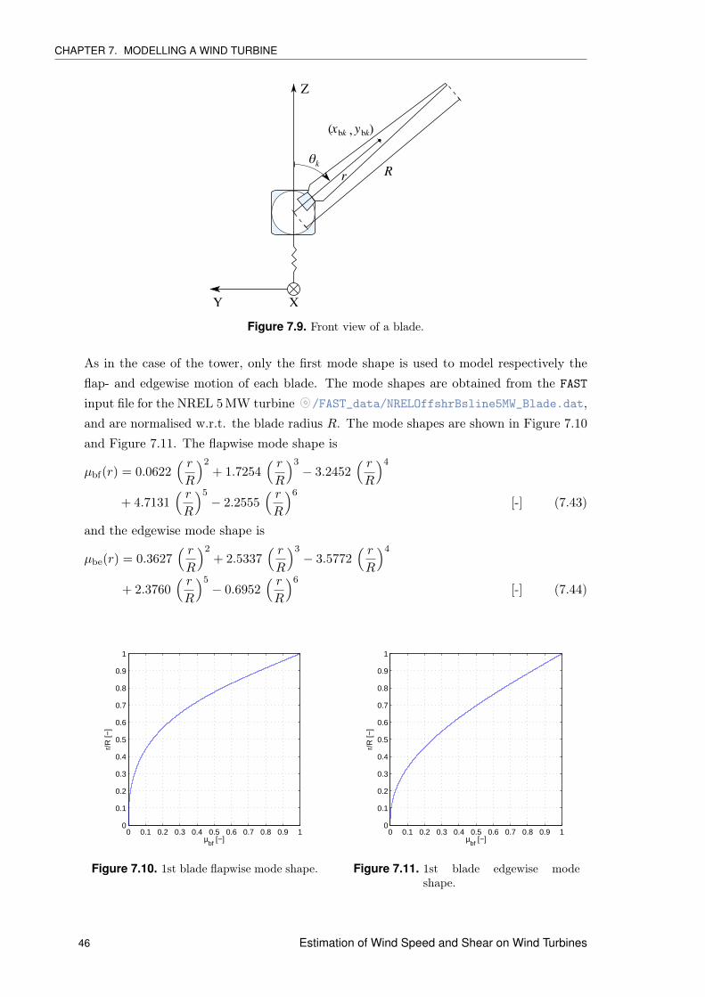
7.5 Blade ModelThe blades of the wind turbine are modelled similar to the tower as a flexible beam with aclamped end and a free end. The motion of the blades is, however more complex becauseof the rotation of the blades. Figure 7.9 illustrates the blade model and the parametersrelated to it.



XY

Z

𝜃

.r

x bk y bk( (,

Rk

Figure 7.9. Front view of a blade.

As in the case of the tower, only the first mode shape is used to model respectively theflap- and edgewise motion of each blade. The mode shapes are obtained from the FAST

input file for the NREL 5 MW turbine /FAST_data/NRELOffshrBsline5MW_Blade.dat,and are normalised w.r.t. the blade radius R. The mode shapes are shown in Figure 7.10and Figure 7.11. The flapwise mode shape is

µbf(r) = 0.0622( rR

)2+ 1.7254

( rR

)3− 3.2452

( rR

)4

+ 4.7131( rR

)5− 2.2555

( rR

)6[-] (7.43)

and the edgewise mode shape is

µbe(r) = 0.3627( rR

)2+ 2.5337

( rR

)3− 3.5772

( rR

)4

+ 2.3760( rR

)5− 0.6952

( rR

)6[-] (7.44)

0 0.1 0.2 0.3 0.4 0.5 0.6 0.7 0.8 0.9 10

0.1

0.2

0.3

0.4

0.5

0.6

0.7

0.8

0.9

1

µbf

[−]

r/R

[−]

Figure 7.10. 1st blade flapwise mode shape.

0 0.1 0.2 0.3 0.4 0.5 0.6 0.7 0.8 0.9 10

0.1

0.2

0.3

0.4

0.5

0.6

0.7

0.8

0.9

1

µbf

[−]

r/R

[−]

Figure 7.11. 1st blade edgewise modeshape.


7.5. BLADE MODEL

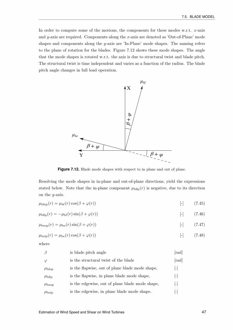
In order to compute some of the motions, the components for these modes w.r.t. x-axisand y-axis are required. Components along the x-axis are denoted as ’Out-of-Plane’ modeshapes and components along the y-axis are ’In-Plane’ mode shapes. The naming refersto the plane of rotation for the blades. Figure 7.12 shows these mode shapes. The anglethat the mode shapes is rotated w.r.t. the axis is due to structural twist and blade pitch.The structural twist is time independent and varies as a function of the radius. The bladepitch angle changes in full load operation.

β + φY

β +

φ

β + φ

Xµbf

µbe

Figure 7.12. Blade mode shapes with respect to in plane and out of plane.

Resolving the mode shapes in in-plane and out-of-plane directions, yield the expressionsstated below. Note that the in-plane component µbfip(r) is negative, due to its directionon the y-axis.

µbfop(r) = µbf(r) cos(β + ϕ(r)) [-] (7.45)

µbfip(r) = −µbf(r) sin(β + ϕ(r)) [-] (7.46)

µbeop(r) = µbe(r) sin(β + ϕ(r)) [-] (7.47)

µbeip(r) = µbe(r) cos(β + ϕ(r)) [-] (7.48)

where

β is blade pitch angle [rad]

ϕ is the structural twist of the blade [rad]

µbfop is the flapwise, out of plane blade mode shape, [-]

µbfip is the flapwise, in plane blade mode shape, [-]

µbeop is the edgewise, out of plane blade mode shape, [-]

µbeip is the edgewise, in plane blade mode shape. [-]



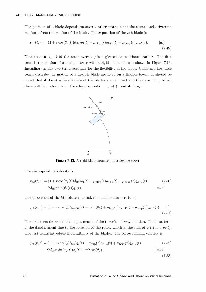
The position of a blade depends on several other states, since the tower- and drivetrainmotion affects the motion of the blade. The x-position of the kth blade is

xbk(t, r) = (1 + r cos(θk(t))δtfa)q1(t) + µbfop(r)qk+4(t) + µbeop(r)qk+7(t), [m]

(7.49)

Note that in eq. 7.49 the rotor overhang is neglected as mentioned earlier. The firstterm is the motion of a flexible tower with a rigid blade. This is shown in Figure 7.13.Including the last two terms accounts for the flexibility of the blade. Combined the threeterms describe the motion of a flexible blade mounted on a flexible tower. It should benoted that if the structural twists of the blades are removed and they are not pitched,there will be no term from the edgewise motion, qk+7(t), contributing.

X Y

Z

q1

rcos( )𝜃k

δ tfa

Figure 7.13. A rigid blade mounted on a flexible tower.

The corresponding velocity is

xbk(t, r) = (1 + r cos(θk(t))δtfa)q1(t) + µbfop(r)qk+4(t) + µbeop(r)qk+7(t) (7.50)

− Ωδtfar sin(θk(t))q1(t), [m/s]

The y-position of the kth blade is found, in a similar manner, to be

ybk(t, r) = (1 + r cos(θk)δtss)q2(t) + r sin(θk) + µbfip(r)qk+4(t) + µbeip(r)qk+7(t), [m]

(7.51)

The first term describes the displacement of the tower’s sideways motion. The next termis the displacement due to the rotation of the rotor, which is the sum of q3(t) and q4(t).The last terms introduce the flexibility of the blades. The corresponding velocity is

ybk(t, r) = (1 + r cos(θk)δtss)q2(t) + µbfip(r)qk+4(t) + µbeip(r)qk+7(t) (7.52)

− Ωδtssr sin(θk(t))q2(t) + rΩ cos(θk), [m/s](7.53)


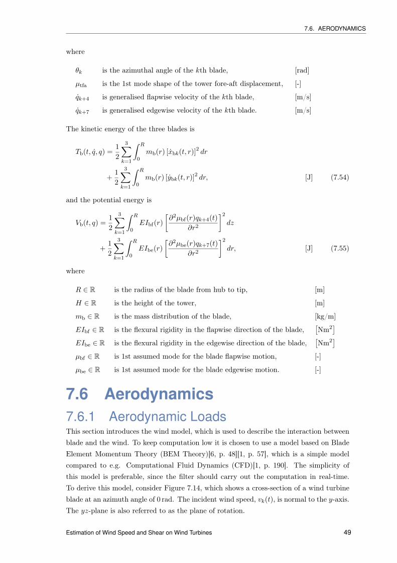
7.6. AERODYNAMICS

where

θk is the azimuthal angle of the kth blade, [rad]

µtfa is the 1st mode shape of the tower fore-aft displacement, [-]

qk+4 is generalised flapwise velocity of the kth blade, [m/s]

qk+7 is generalised edgewise velocity of the kth blade. [m/s]

The kinetic energy of the three blades is

Tb(t, q, q) =1

2

3∑k=1

∫ R

0mb(r) [xbk(t, r)]

2 dr

+1

2

3∑k=1

∫ R

0mb(r) [ybk(t, r)]

2 dr, [J] (7.54)

and the potential energy is

Vb(t, q) =1

2

3∑k=1

∫ R

0EIbf(r)

[∂2µbf(r)qk+4(t)

∂r2

]2

dz

+1

2

3∑k=1

∫ R

0EIbe(r)

[∂2µbe(r)qk+7(t)

∂r2

]2

dr, [J] (7.55)

where

R ∈ R is the radius of the blade from hub to tip, [m]

H ∈ R is the height of the tower, [m]

mb ∈ R is the mass distribution of the blade, [kg/m]

EIbf ∈ R is the flexural rigidity in the flapwise direction of the blade,[Nm2

]EIbe ∈ R is the flexural rigidity in the edgewise direction of the blade,

[Nm2

]µbf ∈ R is 1st assumed mode for the blade flapwise motion, [-]

µbe ∈ R is 1st assumed mode for the blade edgewise motion. [-]

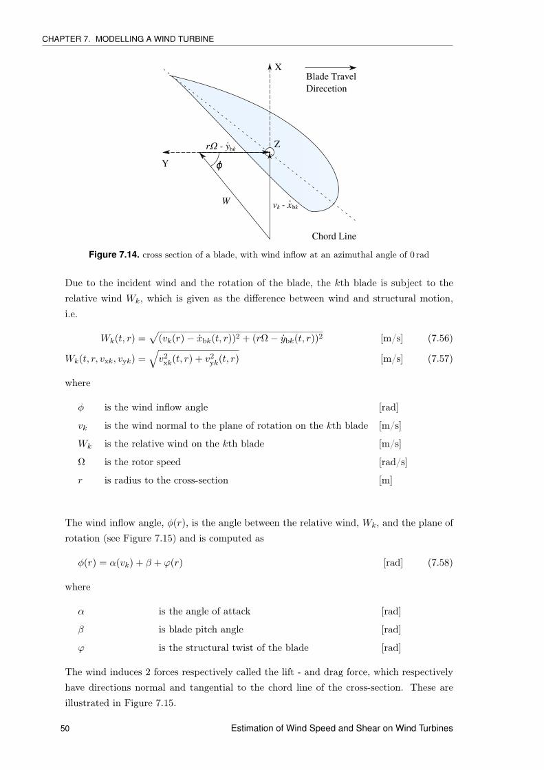
7.6 Aerodynamics7.6.1 Aerodynamic LoadsThis section introduces the wind model, which is used to describe the interaction betweenblade and the wind. To keep computation low it is chosen to use a model based on BladeElement Momentum Theory (BEM Theory)[6, p. 48][1, p. 57], which is a simple modelcompared to e.g. Computational Fluid Dynamics (CFD)[1, p. 190]. The simplicity ofthis model is preferable, since the filter should carry out the computation in real-time.To derive this model, consider Figure 7.14, which shows a cross-section of a wind turbineblade at an azimuth angle of 0 rad. The incident wind speed, vk(t), is normal to the y-axis.The yz-plane is also referred to as the plane of rotation.



X

Y

Z

W

Chord Line

ϕ

rΩ - y

Blade TravelDirecetion

.bk

v - x. bkk

Figure 7.14. cross section of a blade, with wind inflow at an azimuthal angle of 0 rad

Due to the incident wind and the rotation of the blade, the kth blade is subject to therelative wind Wk, which is given as the difference between wind and structural motion,i.e.

Wk(t, r) =√

(vk(r)− xbk(t, r))2 + (rΩ− ybk(t, r))2 [m/s] (7.56)

Wk(t, r, vxk, vyk) =√v2

xk(t, r) + v2yk(t, r) [m/s] (7.57)

where

φ is the wind inflow angle [rad]

vk is the wind normal to the plane of rotation on the kth blade [m/s]

Wk is the relative wind on the kth blade [m/s]

Ω is the rotor speed [rad/s]

r is radius to the cross-section [m]

The wind inflow angle, φ(r), is the angle between the relative wind, Wk, and the plane ofrotation (see Figure 7.15) and is computed as

φ(r) = α(vk) + β + ϕ(r) [rad] (7.58)

where

α is the angle of attack [rad]

β is blade pitch angle [rad]

ϕ is the structural twist of the blade [rad]

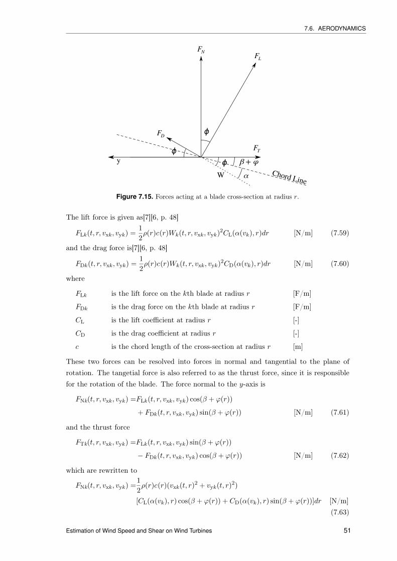
The wind induces 2 forces respectively called the lift - and drag force, which respectivelyhave directions normal and tangential to the chord line of the cross-section. These areillustrated in Figure 7.15.


7.6. AERODYNAMICS

ϕ

ϕ

ϕ β + φ

α

FN FL

FD

yChord Line

FT

W

Figure 7.15. Forces acting at a blade cross-section at radius r.

The lift force is given as[7][6, p. 48]

FLk(t, r, vxk, vyk) =1

2ρ(r)c(r)Wk(t, r, vxk, vyk)

2CL(α(vk), r)dr [N/m] (7.59)

and the drag force is[7][6, p. 48]

FDk(t, r, vxk, vyk) =1

2ρ(r)c(r)Wk(t, r, vxk, vyk)

2CD(α(vk), r)dr [N/m] (7.60)

where

FLk is the lift force on the kth blade at radius r [F/m]

FDk is the drag force on the kth blade at radius r [F/m]

CL is the lift coefficient at radius r [-]

CD is the drag coefficient at radius r [-]

c is the chord length of the cross-section at radius r [m]

These two forces can be resolved into forces in normal and tangential to the plane ofrotation. The tangetial force is also referred to as the thrust force, since it is responsiblefor the rotation of the blade. The force normal to the y-axis is

FNk(t, r, vxk, vyk) =FLk(t, r, vxk, vyk) cos(β + ϕ(r))

+ FDk(t, r, vxk, vyk) sin(β + ϕ(r)) [N/m] (7.61)

and the thrust force

FTk(t, r, vxk, vyk) =FLk(t, r, vxk, vyk) sin(β + ϕ(r))

− FDk(t, r, vxk, vyk) cos(β + ϕ(r)) [N/m] (7.62)

which are rewritten to

FNk(t, r, vxk, vyk) =1

2ρ(r)c(r)(vxk(t, r)

2 + vyk(t, r)2)

[CL(α(vk), r) cos(β + ϕ(r)) + CD(α(vk), r) sin(β + ϕ(r))]dr [N/m]

(7.63)



and

FTk(t, r, vxk, vyk) =1

2ρ(r)c(r)(vxk(t, r)

2 + vyk(t, r)2)

[CL(α(vk), r) sin(β + ϕ(r))− CD(α(vk), r) cos(β + ϕ(r))]dr [N/m]

(7.64)

The derivatives w.r.t. the winds vxk and vyk and the pitch β are required for thelinearisation of the aerodynamic. The derivative of FN w.r.t. vxk is

fNvxk(r) =∂FNk

∂vxk

=1

2ρ(r)c(r) [2vkCL(α(vk), r) cos(β + ϕ(r)) + CD(α(vk), r) sin(β + ϕ(r))]

+ rΩ

(∂CL(α(vk), r)

∂α(vk)+ CD(α(vk), r)

)cos(β + ϕ(r))

+ rΩ

(∂CD(α(vk), r)

∂α(vk)− CL(α(vk), r)

)sin(β + ϕ(r))dr [Ns/m]

(7.65)

The derivative in equation eq. 7.65 have been simplified using the assumption thatW ≈ Ωr

and ∂φ∂v ≈

1Ωr , which are justified in [1, p. 225]. The remaining partial derivatives are found

in [20, p. 57].

7.6.2 Wind ModelThe wind needs to be modelled, such that it is possible to estimate it by different termsin the estimation scheme. It is chosen to describe the wind by the 3 terms of contributionbeing; mean wind speed in hub height, the vertical wind shear and the contribution fromtower shadow. Thereby the wind is modelled as

vk(t) = vH(t) + vwsk(t) + vtsk(t) [m/s] (7.66)

where

vk is the total wind experienced by kth blade [m/s]

vH is the wind speed at hub height [m/s]

vwsk is the wind shear component [m/s]

vtsk is the tower shadow component [m/s]

The components of wind shear, and tower shadow are modelled individually in thefollowing

7.6.3 Wind Shear ModelFor the vertical wind shear to be taken into account a model for this is needed. This shearcan be modelled in many ways, varying in complexity, dependent on e.g. the topography


7.6. AERODYNAMICS

in the particular area where the shear should be calculated. A commonly used model forthe vertical wind shear is seen in equation 7.67[16].

v(z) = vH

( zH

)σ, [m/s] (7.67)

where

z is the height, [m]

H is the hub height, [m]

v(z) is the wind speed at the height z, [m/s]

vH is the wind speed at the hub height, [m/s]

σ is the wind shear coefficient. [-]

𝜃

H

z = r cos(𝜃) + H

r

r0

a

x

1

𝜃2

𝜃3

Figure 7.16. Definitions on the parameters used in the wind model.

From figure 7.16 some of the dimensions and variables used onwards are illustrativelydefined. Then the formula 7.67 can be rewritten as 7.69.

v(r, θk) = vH

(r cos(θk) +H

H

)σ[m/s] (7.68)

= vH

(1 +

r cos(θk)

H

)σ[m/s] (7.69)



Figure 7.17 illustrates the effect of the wind shear at the tip of a blade (r =

63 m) as a function of the azimuthal angle of the kth blade θk as described byequation 7.69 under the conditions stated in table 7.2. The values are inspired bythe FAST documentation /FAST_documentation/Definition of a 5-MW Reference

Wind Turbine for Offshore System Development.pdf, and the value for the windshear coefficient from [16]. The reason for setting r = R is to observe the total change inwind speed from the blade being in top position to being in lowest position.

Parameter Value Unit Description

r 63 [m] radial distance on blade from rotor axisR 63 [m] total length of blader0 1.5 [m] radial distance from rotor axis to blade rootH 90 [m] hub heightvH 10 [m/s] wind speed at hub heightσ 0.14 [-] wind shear coefficientx 5.02 [m] distance from blade to tower midlinea 2.74 [m] tower radius in height H −R

Table 7.2. Conditions set for illustration of wind shear and tower shadow.

0 pi/2 pi 3pi/2 2pi8

8.5

9

9.5

10

10.5

11

Blade azimuth angle [rad]

Win

d sp

eed

[m/s

]

Figure 7.17. Wind shear illustration.

This expression is nonlinear and as the model is linear, this particular model can not bereadily implemented. In [21] by Dolan and Lehn, this model can be expressed as a 3rdorder taylor expansion. The used model for the wind shear is this derived model (equation7.70), which sums up the integration of the wind speed components over the radius of all3 blades.

vws =2vH

3sR2

3∑k=1

∫ R

r0

[r2σ

Hcos θk +

r3σ(σ − 1)

2H2cos2 θk +

r4σ(σ − 1)(σ − 2)

6H3cos3 θk

]dr, [m/s]

=2vH

3sR2

3∑k=1

[(R3σ

3Hcos θk +

R4σ(σ − 1)

8H2cos2 θk +

R5σ(σ − 1)(σ − 2)

30H3cos3 θk

)−(r3

0σ

3Hcos θk +

r40σ(σ − 1)

8H2cos2 θk +

r50σ(σ − 1)(σ − 2)

30H3cos3 θk

)](7.70)


7.6. AERODYNAMICS

with

s , 1−(r0

R

)2

where

vH is the wind speed at the hub height, [m/s]

H is the hub height, [m]

σ is the wind shear coefficient, [-]

θk is the angle of the kth blade, [rad]

r0 is the distance at which the blade profile begins, [m]

r is radial distance from rotor axis, [m]

R is the total length of the blade. [m]

7.6.4 Tower ShadowThe tower shadow contributes to the wind model as well, and the model used in thisproject is, as well as the wind shear model, borrowed from the model derived in [21] andis formulated as in equation 7.71. As there is no tower above the nacelle, the model isonly valid in the interval θk ∈ [π2 ; 3π

2 ].

vts =2mVH3sR2

3∑k=1

[a2ln(R2 sin2 θk + x2)

2 sin2 θk− a2ln(r2

0 sin2 θk + x2)

2 sin2 θk

+a2x2

sin2 θk(R2 sin2 θk + x2)− a2x2

sin2 θk(r20 sin2 θk + x2)

][m/s] (7.71)

with

m , 1 +σ(σ − 1)R2

8H2

where

a is the radius of the tower [m]

x is the distance from tower midline to the blade (overhang) [m]

Figure 7.18 illustrates the contribution to the wind model from the tower shadow for thekth blade, under the conditions listed in table 7.2.



pi/2 pi 3pi/2−1.4

−1.2

−1

−0.8

−0.6

−0.4

−0.2

0

0.2

Blade azimuth angle [rad]

Win

d sp

eed

[m/s

]

Figure 7.18. Tower shadow illustration

7.7 Derivation ExampleThe four subsystems of the wind turbine have now been described. An example of thederivations of mass, stiffness, etc. done in this project, is now presented. This example isintended to make the derivation procedure more obvious and also to show the extent ofthe derivations done in this work, since a large amount of the project time was investedin the derivations of the model.

In this example only the tower fore-aft displacement, q1(t), is considered, which yieldsthe entries of the first row in the mass, stiffness and damping matrices. Consider theEuler-Lagrange equation from eq. 7.4, now only with partial derivatives w.r.t. the towerfore-aft displacement, yielding

0 =d

dt

(∂L(t, q, q)

∂q1

)− ∂L(t, q, q)

∂q1+∂F(t, q)

∂q1− Q1(t) [N] (7.72)

Equation 7.72 represents the first of 10 equations, which describe the wind turbine model.The structural stiffness related to the fore-aft motion is derived by considering the secondterm on the right hand side.

7.7.1 Structural StiffnessThe second term of eq. 7.72 is split into the following terms

− ∂L(t, q, q)

∂q1= −∂T (t, q, q)

∂q1+∂V (t, q)

∂q1[N] (7.73)

It should be noted that T(t) and V(t) are all the kinetic and potential energies in thesystem, not only for the tower. The structural stiffness is then found by taking the partialderivative of V (t, q) w.r.t. q1(t). Since only equation 7.30(on prefeq:tower_pot_energy2)depends on q1(t), it is only necessary to derive w.r.t. this energy contribution, whichyields

∂V (t, q)

∂q1=

(∫ H

0EItfa(z)

[∂2µtfa(z)

∂z2

]2

dz

)q1(t) [N] (7.74)


7.7. DERIVATION EXAMPLE

from which the structural stiffness is found to be

k11s =

∫ H

0EItfa(z)

[∂2µtfa(z)

∂z2

]2

dz [N/m] (7.75)

The only kinetic energy that depends on q1(t) is the kinetic energy of the blade 7.54(onpage 49). Hence the derivative w.r.t. qi1 is

−∂T (t, q, q)

∂q1=

−Ω2δ2tfa

3∑k=1

(∫ R

0mb(r)r2 sin(θk(t))

2dr

)q1(t) (7.76)

+Ωδtfa

3∑k=1

(∫ R

0mb(r)[1 + r cos(θk(t))δtfa]r sin(θk(t))dr

)q1(t) (7.77)

+Ωδtfa

3∑k=1

(∫ R

0mb(r)µbfop(r)r sin(θk(t))dr

)qk+4(t) (7.78)

+Ωδtfa

3∑k=1

(∫ R

0mb(r)µbeop(r)r sin(θk(t))dr

)qk+7(t) [N] (7.79)

All of these terms from the kinetic energy are however cancelled out when considering thefirst term of eq. 7.72.

7.7.2 Mass and Gyroscopic DampingThe potential energy does not depend on the generalised velocity, so the first term of 7.72is reduced to

d

dt

(∂L(t, q, q)

∂q1

)=

d

dt

(∂T (t, q, q)

∂q1

)[N] (7.80)

In this example, the total kinetic energy has two contributions depending on q1(t). Thatis the kinetic energy of the tower and the nacelle and the kinetic energy of the blades.These are respectively eq. 7.28 on page 42 and eq. 7.54 on page 49. The term related toybk(t, r), in eq. 7.54, is independent on the fore-aft motion and is therefore left out in this



example. The derivative w.r.t. q1(t) is

d

dt

(∂T (t, q, q)

∂q1

)=

(∫ H

0mt(z)µtfa(z)2dz +Mn

)q1(t) (7.81)

+3∑

k=1

(∫ R

0mb(r)[1 + r cos(θk(t))δtfa]2dr

)q1(t) (7.82)

+3∑

k=1

(∫ R

0mb(r)[1 + r cos(θk(t))δtfa]µbfop(r)dr

)qk+4(t) (7.83)

+

3∑k=1

(∫ R

0mb(r)[1 + r cos(θk(t))δtfa]µbeop(r)dr

)qk+7(t) (7.84)

−2Ωδtfa

3∑k=1

(∫ R


)q1(t) (7.85)

−Ω2δtfa

3∑k=1

(∫ R

0mb(r)[1 + r cos(θk(t))δtfa]r cos(θk(t))dr

)q1(t) (7.86)

+Ω2δ2tfa

3∑k=1

(∫ R

0mb(r)r2 sin(θk(t))

2dr

)q1(t) (7.87)

−Ωδtfa

3∑k=1

(∫ R


)q1(t) (7.88)

−Ωδtfa

3∑k=1

(∫ R

0mb(r)µbfop(r)r sin(θk(t))dr

)qk+4(t) (7.89)

−Ωδtfa

3∑k=1

(∫ R

0mb(r)µbeop(r)r sin(θk(t))dr

)qk+7(t) (7.90)

The first term stems from the kinetic energy of the tower, while the remaining terms arefrom the kinetic energy of the blades. The last 4 terms,7.87 to 7.90 , cancel out with the4 terms 7.76 to 7.79 from ∂T (t,q,q)

∂q1. The terms 7.81 to 7.84 are entries of the mass matrix

and are expressed as

m11 =

∫ H

0mt(z)µtfa(z)2dz +Mn +

3∑k=1

∫ R

0mb(r)[1 + r cos(θk(t))δtfa]2dr. [kg]

(7.91)

In the case where k = 1, i.e. for the first blade, the term 7.83 yields the mass coefficient

m15 =

∫ R

0mb(r)[1 + r cos(θ1(t))δtfa]µbfop(r)dr, [kg] (7.92)

and for k = 1 term 7.84 yields the coefficient

m18 =

∫ R

0mb(r)[1 + r cos(θ1(t))δtfa]µbeop(r)dr. [kg] (7.93)

Term 7.85 depends on the generalised velocity of the tower and is regarded as dampingdue to gyroscopic loads. This damping is denoted as

c11g = −2Ωδtfa

3∑k=1

∫ R

0mb(r)[1 + r cos(θk(t))δtfa]r sin(θk(t))dr. [Ns/m] (7.94)


7.7. DERIVATION EXAMPLE

The damping of the wind turbine therefore consists of structural-, aerodynamic- andgyroscopic damping, i.e.

cij = cijs + cija + cijg. [Ns/m] (7.95)

Term 7.86 depends on the generalised coordinate of the tower and is regarded as additionalstiffness due to centrifugal loading on the blades. This stiffness is denoted as

k11c = −Ω2δtfa

3∑k=1

∫ R

0mb(r)[1 + r cos(θk(t))δtfa]r cos(θk(t))dr. [N/m] (7.96)

The total stiffness of the wind turbine therefore consists of structural-, gravity induced-and centrifugal stiffness, i.e.

kij = kijs + kijg + cijc. [N/m] (7.97)

7.7.3 Aerodynamic DampingAs shown in the introduction of this chapter, the ijth entry of the aerodynamic dampingis given as

cija =3∑

k=1

∫ R

0

∂xbk

∂qi

[∂FNk

∂vxk

∂vxk

∂qj+∂FNk

∂vyk

∂vyk

∂qj

]+∂ybk

∂qi

[∂FTk

∂vxk

∂vxk

∂qj+∂FTk

∂vyk

∂vyk

∂qj

]dr [-] .

(7.98)

Remembering that the equations for the kth blade’s motion are

xbk(t, r) = (1 + r cos(θk(t))δtfa)q1(t) + µbfop(r)qk+4(t) + µbeop(r)qk+7(t), [m]

(7.99)

xbk(t, r) = (1 + r cos(θk(t))δtfa)q1(t) + µbfop(r)qk+4(t) + µbeop(r)qk+7(t) (7.100)

− Ωδtfar sin(θk(t))q1(t), [m/s](7.101)

and

ybk(t, r) = (1 + r cos(θk)δtss)q2(t) + r sin(θk) + µbfip(r)qk+4(t) + µbeip(r)qk+7(t), [m]

(7.102)

ybk(t, r) = (1 + r cos(θk)δtss)q2(t) + µbfip(r)qk+4(t) + µbeip(r)qk+7(t) (7.103)

− Ωδtssr sin(θk(t))q2(t) + rΩ cos(θk), [m/s](7.104)

The wind normal to the plane of rotation is given as

vxk = vk − xbk(t, r), [m/s] (7.105)



and the wind parallel to plane of rotation is

vyk = rΩ− ybk(t, r), [m/s] (7.106)

The aerodynamic damping is now computed using the former 6 equations. The derivationsfor the first 2 aerodynamic damping coefficients are now presented.

∂xbk

∂q1= 1 + r cos(θk)δtfa

∂ybk

∂q1= 0

∂FNk

∂vxk= fNvxk(r)

∂FNk

∂vyk= fNvyk(r)

∂vxk

∂q1= −(1 + r cos(θk)δtfa)

∂vyk

∂q1= 0

Combining the derivatives yields

c11a = −3∑

k=1

∫ R

0(1 + r cos(θk)δtfa)2fNvxk(r)dr [Ns/m]

The derivatives for the next coefficient are

∂xbk

∂q1= 1 + r cos(θk)δtfa

∂ybk

∂q1= 0

∂FNk

∂vxk= fNvxk(r)

∂FNk

∂vyk= fNvyk(r)

∂vxk

∂q2= 0

∂vyk

∂q2= −δtssr

which yields

c12a = −3∑

k=1

∫ R

0(1 + r cos(θk)δtfa)fNvyk(r)δtssrdr [Ns/m]

This is an example of how to derive 2 of the entries of the aerodynamic damping matrix.This matrix is not symmetric and therefore consists of almost 100 equations to define allthe entries. The negative sign on the entries are cancelled by the negative sign on theaerodynamic damping matrix, so this phenomenon adds more damping to the system.

Remark 1 The formula used is the same as in the used source[20]. However the resultsobtained here are not the same as in the used literature. Therefore all the 100 entries forthe aerodynamic damping matrix C has been derived in appendix B.3

7.7.4 Structural DampingThe derivative of the dissipation function is considered to derive the structural damping.

∂F(t, q)

∂q1= c11sq1(t) = 2ζ1

√k11m11q1(t) [N] (7.107)


7.8. PARAMETER DISTRIBUTIONS

and the structural damping is therefore

c11s = 2ζ1

√k11m11, [Ns/m] (7.108)

The mass and stiffness coefficient are compute and the damping factor ζ1 = 0.01 are fromthe FAST input file /FAST_data/NRELOffshrBsline5MW_Tower_Onshore.dat.

The derivation of the total model is quite big. The presented example representsapproximately 1/10th of the total number of equations, which forms the final model ofthe wind turbine. However, since the approach now should be more obvious, then theremaining equations are placed in an appendix. They are found in Appendix B.1 onpage 111.

7.8 Parameter DistributionsThe parameters for usage in the developed model are for the tower and blades given interms of distributed parameters.

For computation of the model, it is convenient to have a function describing thebehaviour of these parameters as a function of height and radius for respectively thetower and the blades. Therefore the parameters are interpolated in MATLAB, using 1storder splines between each point from the input file to obtain a first order linear function.

An example is the mass distribution for the tower. In the Figure 7.19 the data fromthe FAST input file is plotted as the black dots, and the interpolated function is plottedalongside being the blue curve.

0 10 20 30 40 50 60 70 80 902500

3000

3500

4000

4500

5000

5500

6000

Tower Height [m]

Tow

er M

ass

[kg/

m]

datafitted curve

Figure 7.19. Mass distribution of the tower.

In 7.109 the mass distribution is listed as a function of the height z.



mt(z) =

5590.870000− 40.91780822 z z< 8.76

5579.100000− 39.57420091 z z< 17.52

5555.540000− 38.22945205 z z< 26.28

5520.230000− 36.88584475 z z< 35.04

5473.110000− 35.54109589 z z< 43.80

5414.310000− 34.19863014 z z< 52.56

5343.630000− 32.85388128 z z< 61.32

5261.170000− 31.50913242 z z< 70.08

5167.090000− 30.16666667 z z< 78.84

5061.070000− 28.82191781 z otherwise

[kg/m] (7.109)

The used input data file is found on the enclosed CD /FAST_data/. Thedistributed parameters describing mass and stiffness of the tower are obtained from/FAST_data/NRELOffshrBsline5MW_Tower_Onshore.dat. The distributed parameters

describing mass, flexural rigidity, structural twist of the blades are obtained from/FAST_data/NRELOffshrBsline5MW_Blade.dat. All the used distributed structural

parameters are treated likewise, and the results are found in appendix AAerodynamic data in terms of the Lift and Drag coefficients alongside with inflow

angle are obtained from /FAST_data/NRELOffshrBsline5MW_AeroDyn.ipt. The inflowangle, Lift and drag coefficients alongside with derivatives w.r.t. angle of attack aredescribed in appendix A.3, where a calculation example is given.

7.9 State Space FormulationThe equations, which describes the dynamics of the wind turbine as an LPV system aregiven in matrix form as

M(θ)q(t) + C(θ)q(t) +K(θ)q(t) = Qββ(t) +Qττ(t) +Qvv(t), (7.110)

which leads to

q(t) = M(θ)−1 (−C(θ)q(t)−K(θ)q(t) +Qβ(θ)β(t) +Qττ(t) +Qv(θ)v(t)) (7.111)


7.9. STATE SPACE FORMULATION

The matrix equation, 7.111, for the generalised accelerations is used to formulate thesystem in state space form, which isq(t)

q(t)

=

0 I

−M(θ)−1K(θ) −M(θ)−1C(θ)

q(t)q(t)

+

0 0

M(θ)−1Qβ(θ) M(θ)−1Qτ

β(t)

τ(t)

+

0

M(θ)−1Qv(θ)

v(t). (7.112)

In a shorter notation the state space system is

x(t) = A(θ)x(t) +B(θ)u(t) + E(θ)d(t) (7.113)

where

A ∈ R20×20 is the state transition matrix [-]

B ∈ R20×4 is the gain of the control inputs [-]

E ∈ R20×3 is the gain of the wind disturbance [-]

The state vector x(t) is

x(t) =

q(t)q(t)

, x(t) =

q(t)q(t)

The input vector u(t) contains the blade pitch on each blade, βi(t), for i = 1, 2, 3, and theapplied generator torque, τ(t)

u(t) =[β1(t) β2(t) β3(t) τ(t)

]T, (7.114)

The disturbance d(t) is the wind speed on each blade

d(t) =[v1(t) v2(t) v3(t)

]T. (7.115)

For simulation purpose, the continues-time system eq. 7.113 is discretied using a zero-order-hold transformation. The discrete-time system is denoted as

xs(k + 1) = Φs(θ)xs(k) + Γs(θ)u(k) + Γd(θ)d(k) (7.116)

This discrete model is used when simulating the model and for implementing in theestimator. However a modification to the model is carried out in order to avoidcomputational problems. The state describing the angular displacement of the generator,q3(t), is excluded, since it is constantly increasing i.e. an unstable mode.


8 Estimating WindThis chapter is meant to give an overview of the various considerations made, whendesigning the estimation scheme for wind speed and wind shear. First a brief outlineof the different sensor types and their pros and cons in the specific setup alongside witha justification, why these sensors specifically have been chosen to consider. Finally, theestimation strategy is presented and the implementation of this on the model derived inthe previous chapter is undergone.

8.1 Sensor TypesThere are different types of sensors considerable for measurements that can be used forestimating the wind fields. The sensors considered in this project are briefly describedbelow. It should be noted that this project does not focus on the full derivation frommeasurements to deflection data used in the estimation scheme, hence only the idea ofwhich sensors could be used for the purpose with no further development, is presented

8.1.1 Strain GaugesA strain gauge is a stretchable sensor which, dependent on the strain it is subject to, givesa corresponding output. The sensor often consist of a very thin metal wire, which due toits thickness is stretchable within a certain range. As the length of the wire is increased,the resistance in the wire increases as well, and vice versa for a decrease in length. In thematter of this project, this means that one or several sensors would be attached on eachblade and on the tower. In this way, it is possible to measure the bending of the bladesand the tower, and thereby determine the wind force on each of these elements. Usingstrain gauges on blades and tower is already a configuration in some wind turbines [12].

One of the advantages of using strain gauges is that they are easily implementable on thewind turbine.

Another advantage of using strain gauges is that the output is fairly easy to convertto force applied from the wind if the mode shapes of the blade is known. However, as thepractical implementation of this conversion is not part of this master project, this is notfurtherer considered.

A disadvantage of the strain gauge is that the voltage output is very low (measures inmV). In combination with high amplitude vibrations, which are known to occur on thewind turbine, especially on the wings, the reliability and accuracy of the sensor output

65

CHAPTER 8. ESTIMATING WIND

decreases.Another disadvantage of the strain gauge is that due to its thickness, it is very

sensitive to temperature changes. On modern multi megawatt wind turbines, thetemperature is not the same in top position as it is in bottom position. The temperatureexperienced varies as well as a function of rotation speeds, why this makes this sensortype unsuitable for the purpose.

The strain gauge comes in a great span of variants though, and some of these canwithstand the before mentioned disadvantages. However, as the performance goes up, sodoes the price[22].

8.1.2 AccelerometersAccelerometers could be placed along the tower and the blades in cooperation with thestrain gauges. From the accelerations measured and the assumed mode shapes for thewind turbine’s tower and blades respectively, alongside with a start position measuredfrom the strain gauge, the deflection of the tower can be determined from integrating overthe accelerometer data. From this, the wind force on the different parts can be determined,and thereby wind speed and -direction.

One of the advantages of using the accelerometers, is that many wind turbines alreadycontains at least one accelerometer in the tower and one in each blade as well[12], whythe implementation would be simple in comparison to installing new sensors on each windturbine.

A disadvantage of using accelerometers is that if it is not sufficient with only oneaccelerometer on the tower and one on each blade, the implementation of more is not assimple a task as for the strain gauges, since accelerometers most often must be calibratedfor the specific setup. These calibrations includes biasing, drifting etc.

8.2 Sensor SetupMore sensors, such as flowmeters have been considered, however as the disadvantagesof using such are so dominant in comparison to the two above described it is chosento only consider these sensors for usage in the estimation scheme for this project. Theis assumed to be the usage of the already implemented accelerometers. This is chosenprimarily because the practical implementation of these is already done, meaning thatthe approach made throughout this project can be implemented with close to no furtherhardware changes on the wind turbine. It is chosen to assume that measurements areobtained from only one accelerometer on each blade and one on the tower, as this is theconfiguration known to already exist on modern wind turbines[12]. The strain gaugeshowever need to be implemented. An idea for this implementation, would be to install


8.3. KALMAN ESTIMATOR

them on the inside of the blades and tower, as this will expose them for the least fatiguefrom surroundings and the weather.

8.3 Kalman EstimatorChapter 7 on page 33 proposed a model for the wind turbine as well as a model for thewind, and how it interacts with the wind turbine. This section describes an approachto estimate the wind speed and the parameters related to the wind shear. Consider thediscrete version of the non-linear dynamics of the wind turbine system formulated in ashort notation as:

xs(k) = f1(xs(k − 1), u(k − 1)). (8.1)

The model for the wind speed, which includes shear and tower shadow as described inchapter 7.6.3 on page 52, is denoted in short as

v(k) = f2(vzH(k − 1), σ(k − 1)). (8.2)

The two parameters describing the wind shear, which are the hub height wind speed andthe power coefficient, are modelled as constants

vzH(k) = vzH(k − 1) (8.3)

σ(k) = σ(k − 1). (8.4)

The system equations are augmented with the model for the wind speed and the shearparameter, such that the augmented state vector becomes

x(k) =[xs(k)T v(k)T vzH(k) σ(k)

]T(8.5)

where

xs ∈ R20 is the state vector,

v ∈ R3 is wind speed on the blades,

vzH ∈ R is the wind speed at hub height,

σ ∈ R is the wind shear coefficient,

x ∈ R25 is the augmented state vector.

From this point on the notation of time is denoted as a subscript. This is done to havea more convenient way of formulating the filter equations. By this, the current state isdenoted xk and the previous state xk−1. The set of non-linear equations, which describethe dynamics of the augmented system are

xk = f(xk−1, uk−1) + wk−1, wk ∼ N (0, Qk) (8.6)


CHAPTER 8. ESTIMATING WIND

and with the sensor dynamics

zk = h(xk) + vk, vk ∼ N (0, Rk). (8.7)

The model is assumed to be subject to the additive, zero-mean, white noise, being theprocess noise w and the sensor noise v. Also the process and sensor noise are assumed tobe uncorrelated, so the covariance is

E

wkvk

[wTk vTk

] =

Qk 0

0 Rk

(8.8)

The estimation error is defined as the difference between the states and the state estimates.

ek = xk − xk|k, (8.9)

with the covariance of the error denoted as

Pk = EekeTk (8.10)

Several estimation methods exist for non-linear systems, e.g. linearised Kalman filter,Extended Kalman Filter (EKF), Unscented Kalman Filter (UKF)[23]. The latter two aremore suitable for this estimation problem due to the non-linearities in the aerodynamics(7.63 and 7.64 on page 52). In these equations, it is seen, that the input of β occur insine- and cosine functions. Also, the relative winds are squared, resulting in non-linearityin the incident wind and generalised velocities. The linearised Kalman filter will deviate,if states and inputs change too much w.r.t. the operating points. The algorithm for theExtended Kalman Filter (EKF)[23, p. 310] is written below. The notation xk|k−1 is usedto denote the kth predicted state given the previous estimate, while xk|k denotes the stateestimate found by correcting the predicted state with the measurement.

Prediction Step:

Predict the current state by using previous state estimates and previous inputs in thenon-linear system equations.

xk|k−1 = f(xk−1|k−1, uk−1) (8.11)

Linearise the system, in the current state prediction, with the Jacobians

Φk = ∂f(xk,uk)∂xk

∣∣∣xk|k−1,uk

(8.12)

Hk = ∂h(xk)∂xk

∣∣∣xk|k−1

(8.13)

Predict the error covariance by propagating a previous estimate through the linearisedsystem and also using statistics of process noise, i.e. the covariance.

Pk|k−1 = ΦkPk−1|k−1ΦTk +Qk−1 (8.14)


8.3. KALMAN ESTIMATOR

Update Step:

Compute the current Kalman gain

Kk = Pk|k−1HTk (HkPk|k−1H

Tk +Rk−1)−1 (8.15)

Estimate states by correcting the prediction with measurements

xk|k = xk|k−1 +Kk(zk − h(xk|k−1)) (8.16)

Estimate the error covariance

Pk|k = (I −KkHk)Pk|k−1 (8.17)

The EKF has the advantage, compared to the linearised Kalman filter, that it handleschanges in e.g. azimuth angle (θ(t) = q3(t) + q4(t)), which varies from 0 to 2π. Adisadvantage of EKF is the linearisation procedure. For the proposed wind turbine model,the expressions for the Jacobians become very large. Especially the linearisation of theaerodynamics gives rise to some problems, i.e. it require some partial derivatives w.r.t.angle of attack and the pitch angle, which are not known. Some assumptions like thosein [7] (see section 7.6.1 on page 49) are made to reduce the expressions e.g. W ≈ Ωr

etc. Likewise, some approximations, need to be calculated e.g. the derivatives of thelift and drag coefficients with respect to the angle of attack. The approximations madeon these in this project are found in A.3. This occurs even for a uniform wind and byextending with the effects of wind shear, tower shadow etc., the derivations gets even morecomplicated. These problems could be avoided by using a UKF instead, where stochasticlinearisation is used instead of Jacobians. The disadvantage of the UKF is that it requiresmore computation than EKF.

It is assumed, that the UKF is the better filter of the 3 for the estimation purpose ofthis project, since the approximations required for calculating the Jacobians are avoided.However in this work, it would be preferable to try out both UKF and EKF in order tocompare the performance of those. If the UKF is not significantly better than the EKF,it would be preferable to use EKF to keep computation complexity low.


9 Implementation OverviewThis chapter covers the implementation of the developed wind turbine model and thedesigned linearised Kalman filter. Due to time limitations, the model was not fully derivedand validated, why it was not suitable for usage in the wind estimator. However themodel developed is, as mentioned in the previously, tested with the linearised azimuthdependent LPV system matrices from FAST, to determine whether or not the modelderived acts correspondingly to the FAST model. Afterwards, the linearised Kalman filter isimplemented on this model and tested to determine if it is capable of estimating the windfield parameters, hub height speed and wind shear coefficient

9.1 Implmentation of the ModelThe developed model, described in chapter 7, was intended to be validated by simulationagainst the National Renewable Energy Laboratory (NREL) 5 MW non-linear windturbine simulator used as benchmark. Afterwards, the output of the turbine simulator,given a set of inputs, would have been compared to the output from the developed model,utilised by simulation of the derived non-linear equitations. However such a model isnot derived and it is therefore chosen to test the model with the matrices from the FAST

linearisation around operating points for rotor speed, hub height wind speed and windshear. The matrices are obtained in accordance to the description in appendix D.

The parameters described in chapter 7.8 are used to compute the linearised mass,stiffness, damping and forcing matrices described in chapter 7, where the followingoperating points are used for linearisation. Rotor speed of 12.1 rpm, collective bladepitch angle of 0 rad and a uniform wind field with a wind speed of 10 m/s. Wind shearand pitch angle are neglected to keep the computation complexity low. The computationsof the matrices are done by usage of Maple in which the equations described in appendixB are computed. The Maple worksheet used for calculating the matrices is found on theCD /model_matrices/model.mw. Note that since the model was not fully developedthe parts which was not developed is taken from [20].

In order to obtain a set of linearised matrices from FAST a linearisation is performedbased on the same parameters and operating points used when calculating the developedmodel[15]. An example of the FAST matrices is given in appendix C alongside withthe corresponding matrices obtained by evaluating the developed model. They are allevaluated at a rotor angle position of 0 rad.

In order to compare the matrices from FAST against the ones from the model, theEuclidean norm is used since it calculates the most dominant singular value in a matrix.The Euclidean norm is described by equation 9.1[24].

71

CHAPTER 9. IMPLEMENTATION OVERVIEW

The Euclidean norm is calculated for matrices evaluated at 0 rad and compared inpercentage deviation from the fast model. The percentage comparison is done by usageof equation 9.2.

‖A‖2 =√λmax(A∗A) = σmax(A) (9.1)

PA =‖Amodel −Afast‖2

‖Afast‖2(9.2)

Where:

A is a given square Matrix

Amodel is a matrix calculated from the derived model

Afast is a matrix obtained by linearisation in FAST

λmax is the largest eigenvalue

σmax is the largest singular value

PA is the percentage that Amodel deviates from Afast

The percentage deviation for the calculated matrices are the following:

• Mass Matrix at 0 degree: PM = 0.18%

• Stifness Matrix at 0 degree: PK = 0.019%

• Damping Matrix at 0 degree PC = 151%

The Mass and Stiffness matrices seem to match the corresponding matrices from FAST,while the damping matrix shows large deviations. In order to have a model for usage inthe estimator it is therefore chosen to use the linearised matrices from FAST onwards in theproject. The way in which the linearised matrices are obtained and used for simulationand comparison with the benchmark NREL 5 MW turbine, is described in appendix D.As is the structure of the linearised model.

9.2 Implementation of the EstimatorIn order to implement a UKF and EKF as described in section 8.3 a non-linear modelwould be needed, however due to time limits a linear model was developed. The usage ofa Kalman filter for estimation of the wind speed and vertical wind shear power exponentis approached by a linear Kalman filter. The equations for this filter are presented in thefollowing. The linearised state space system used is described in appendix D.

The system and disturbance dynamics are described by equation 9.3 and 9.4.

xs(k + 1) = Φs(θ)xs(k) + Γs(θ)u(k) + Γd(θ)d(k) (9.3)

xd(k + 1) = Φdxd(k) (9.4)

d(k) = Hdxd(k) (9.5)


9.2. IMPLEMENTATION OF THE ESTIMATOR

where

xs(k) ∈ R19 is the system state vector

xd(k) ∈ R2 is the disturbance state vector

u(k) ∈ R4 is the control input vector

d(k) ∈ R2 is the disturbance vector

Φs(θ) ∈ R19×19 is the system state transition matrix

Φd(θ) ∈ R2×2 is the disturbance state transition matrix

Γs(θ) ∈ R19×4 is gain of the control inputs

Γd(θ) ∈ R2×2 is gain of the disturbances

Hd ∈ R2×2 is the output disturbance matrix

The discretised system can now be augmented as follows:xs(k + 1)

xd(k + 1)

=

Φs(θ) Γd(θ)Hd

0 Φd

xs(k)

xd(k)

+

Γs(θ)

0

u(k),

x(k + 1) = Φ(θ)x(k) + Γ(θ)u(k)

y(k) = Hx(k)

y(k) =[Hs 019×2

]x(k)

Where:

x(k) ∈ R21 is the augmented state vector

Φ(θ) ∈ R21×21 is the augmented system state transition matrix

Γ(θ) ∈ R21×4 is gain of the control inputs

H ∈ R19×21 is the augmented output matrix

Hs ∈ R19×19 is the system output vector

The wind disturbances is chosen to be modelled as a step, hence Φd(θ) is an identitymatrix. The Kalman filter equations in terms of prediction and update step is, in chapter8.3, described for the Extended Kalman Filter (EKF). These equations also apply tothe linear Kalman filter with the modification that the system is not linearised in everyiteration. Hence the linearisation carried out in the prediction step of the filter, seeequation 8.11, 8.12 and 8.13 on page 68 is not carried out. This means, that in this case,the same FAST linearised matrices are used in every prediction step. The MATLAB files inwhich the Kalman filter is implemented is attached on the enclosed cd /estimator.


10 Acceptance TestThis chapter covers the acceptance test, described on chapter 5, of the requirementsspecified in chapter 4. Following are the results of the tests, and a discussion on theseregarding whether the requirements set in the requirement specification are met. First themodel are tested and afterwards the filter is tested.

10.1 Model ValidationThe validation of the model is carried out at wind speeds below the rated wind speed forthe 5 MW turbine. This is done such that the blade pitch angle is kept at 0 o, which is theoperating point, that the model matrices are linearised about. For the validation of theused model, 3 differently configured models are tested against each other where model #1

is the FAST non-linear turbine model while model #2 and #3 are two different linearisedmodels obtained from FAST linearisation, as described in appendix D. The properties andinclusions for these 3 different models are listed in table 10.1.

Model Blade precone Shaft tilt Rotor overhang Non-linear model

#1 X X X X

#2 ÷ ÷ ÷ ÷#3 X X X ÷

Table 10.1. The three models used for validation.

Model #1 is the benchmark model from FAST, being a non-linear model which takesboth blade precone, rotor shaft tilting, and rotor overhang into account.

Model #2 is a FAST linearised model comparable to the model attempted derived inthis project, which excludes blade precone, rotor shaft tilting, and rotor overhang.

Model #3 is a FAST linearised model that includes blade precone, rotor shaft tiltingand rotor overhang. The reason for constructing and examining this model is to investigatethe the impact of including or excluding the mentioned parameters.

More models could have been made by the means of including respectively bladepreconing, rotor shaft tilting and rotor overhang one at a time, to determine the impactof excluding only some of the dynamics compared to excluding all 3 at the same time.However, it is a time consuming process, why only these 3 models have been made andtested.

The validation is carried out in accordance to the description in appendixD withoperation points set for the linearisation in terms of rotor speed, Ω, of 1.2671 rad/s, hubheight wind speed, v, of 10 m/s and a vertical shear with a power exponent of 0.1.

In order to examine the linearised models’ response, when deviations from the

75

CHAPTER 10. ACCEPTANCE TEST

operating point is imposed, the wind speed is stepped from 10 m/s to 11 m/s after 60 s. InFigure 10.1(a) the wind speed during the simulation is shown alongside with the verticalshear exponent in Figure 10.1(b). The presence of shear causes the operation point valuefor the wind speed of 10 m/s being changed to 9.995 m/s. The NREL 5 MW turbine non-linear simulator, represented by model #1, is run for 120 seconds generating a series ofinput and output data. This input and output data is used for simulating model #2 and#3 and comparing them to model #1.

0 20 40 60 80 100 12010

10.5

11

11.5a: Wind Speed [m/sec]

Time [s]0 20 40 60 80 100 120

0

0.1

0.2

0.3

0.4

b: Vertical Shear [−]

Time [s]

Figure 10.1. Input wind data.

10.1.1 Model #1 vs. Model #2First Model #2 is validated up against #1. Figure 10.2 shows the tower displacementsand the tower displacement velocities for model #1 and model #2. It is seen in theFigure 10.2(a) that the fore-aft displacement has an offset of approximately 0.075 m. It isas well seen in Figure 10.3 which is a close up of the Figure 10.2(b), at around 60 s, wherethe step on the wind speed from 10 m/s to 11 m/s occur, the model #2 starts deviatingmore from the benchmark, both in amplitude, and an increase in delay seems to occur aswell. The deviation in amplitude is explained from the fact that the system matrices usedfor model #2 are linearised around operation points, hence the increase in deviation whenleaving the operation point. The delay is assumed to be caused by some of the excludeddynamics, in terms of the neglected blade precone, rotor shaft tilting and rotor overhang.


10.1. MODEL VALIDATION

0 20 40 60 80 100 1200.2

0.25

0.3

0.35

0.4

0.45

0.5

0.55a: Tower Fore−aft Displacement[m]

Time [s]

model #1 (FAST)model #2

0 20 40 60 80 100 1200

0.01

0.02

0.03

0.04

0.05

0.06

0.07

0.08b: Tower side−side Displacement[m]

Time [s]

0 20 40 60 80 100 120−0.3

−0.2

−0.1

0

0.1

0.2

0.3

0.4c: Tower Fore−Aft Displacement Velocity [m/s]

Time [s]0 20 40 60 80 100 120

−0.08

−0.06

−0.04

−0.02

0

0.02

0.04

0.06

0.08d: Tower Side−side Displacement Velocity [m/s]

Time [s]

Figure 10.2. Tower displacements (#1 vs. #2).

55 60 65 70 750.02

0.025

0.03

0.035

0.04

0.045

0.05

0.055

0.06Tower side−side Displacement[m]

Time [s]


Figure 10.3. Tower displacement side-side (#1 vs. #2) close-up.



Figure 10.4(b) shows that regarding the generator speed, model #2 does not track thebenchmark model, neither before nor after the step. The deviation after the step isexpected, as the wind deviates from its operating point. However as the model #2 alsohere deviates from model #1, before the step, the excluded dynamics seem to have animpact here as well.

0 20 40 60 80 100 12030

32

34

36

38

40

42a: Generator Torque[kNm]

Time [s]

0 20 40 60 80 100 1201.18

1.19

1.2

1.21

1.22

1.23

1.24

1.25

1.26b: Generator Speed (LSS) [rad/s]

Time [s]


Figure 10.4. Generator torque and generator speed (#1 vs. #2).

In Figure 10.5 the drivetrain displacement and displacement velocity for model #1 andmodel #2 are seen. Figure 10.6 shows 2 different close-up intervals of the drivetraindisplacement, Figure 10.5(a). The first interval Figure 10.6(a) shows the displacementbefore the step on the wind speed, and Figure 10.6(b) after the step. Both cases seem tohave some of the same effects as were noticed for the displacement in side-side displacementof the tower, regarding amplitude deviation and a little delay, which both worsen afterthe step as expected.



0 20 40 60 80 100 1203.2

3.4

3.6

3.8

4

4.2

4.4

4.6x 10

−3 a: Drivetrain Displacement[rad]

Time [s]


0 20 40 60 80 100 120−4

−3

−2

−1

0

1

2

3

4x 10

−3 b: Drivetrain Displacement Velocity[rad/sec]

Time [s]

Figure 10.5. Drivetrain displacements (#1 vs. #2).

20 25 30 35 403.485

3.49

3.495

3.5

3.505

3.51

3.515

3.52x 10


Time [s]


80 85 90 95 1004.43

4.432

4.434

4.436

4.438

4.44

4.442

4.444

4.446

4.448x 10

−3 b: Drivetrain Displacement[rad]

Time [s]





Figure 10.7(a) and (b) show respectively the flapwise and edgewise displacement of the3 blades of model #2. It is not possible to conclude anything on this plot alone otherthan the 3 blades seem to behave as intended compared to each other. Figure 10.8(a)on the other hand shows an offset regarding the flapwise displacement of blade 1 frommodel #2 compared to model #1 of approximately 0.25 m and an amplitude deviationof approximately 0.25 m as well. The flapwise displacement velocity (see Figure 10.8(c))deviates as well, as a result of the deviation in the flapwise displacement. It is noticed,that the flapwise displacement and the tower fore-aft displacement both suffer an offset inmodel #2 compared to model #1, which is assumed to be caused mainly by the exclusionof rotor overhang.

0 20 40 60 80 100 1203.5

4

4.5

5

5.5

6a: Blade flap Displacement [m]

Time [s]

model #2 blade 1model #2 blade 2model #2 blade 3

0 20 40 60 80 100 120−0.8

−0.6

−0.4

−0.2

0

0.2

0.4

0.6

0.8b: Blade edge Displacement [m]

Time [s]

Figure 10.7. Blade displacements (#2).



0 20 40 60 80 100 1203.5

4

4.5

5

5.5

6a: Blade flap Displacement[m]

Time [s]0 20 40 60 80 100 120

−0.6

−0.4

−0.2

0

0.2

0.4

0.6

0.8b: Blade edge Displacement[m]

Time [s]

0 20 40 60 80 100 120−1.5

−1

−0.5

0

0.5

1

1.5c: Blade flap Displacement Velocity[m/s]

Time [s]0 20 40 60 80 100 120

−2

−1.5

−1

−0.5

0

0.5

1

1.5

2d: Blade edge Displacement Velocity[m/s]

Time [s]

1. blade model #1 (FAST)1. blade model #2

Figure 10.8. Blade displacements (#1 vs. #2).

10.1.2 Model #1 vs. Model #3Following are the test results from the test of model #3 compared to the benchmarkmodel, i.e. model #1. The idea of this is to determine whether it shows any effect fromincluding the dynamics of; blade preconing, rotor shaft tilting, and rotor overhang on thelinear model. The plots and close-ups presented are for the same intervals as for the testbetween model #1 and model #2 such that it is possible to justify the results one modelover the other.

Figure 10.9 shows the tower displacement for model #1 and model #3. It is seen inFigure 10.9(a) that the offset of approximately 0.075 m, in the interval before the step, isnow gone, and in the close up (Figure 10.10) around and after the step, great improvementsare seen as well, both regarding following of amplitude and frequency. It must be concludedthat including the dynamics that were excluded in model #2 have a great impact on thebehaviour of both the tower fore-aft and side-side displacement.



0 20 40 60 80 100 1200.2

0.25

0.3

0.35

0.4

0.45

0.5a: Tower Fore−aft Displacement[m]

Time [s]


0 20 40 60 80 100 1200

0.01

0.02

0.03

0.04

0.05

0.06

0.07

0.08b: Tower side−side Displacement[m]

Time [s]

0 20 40 60 80 100 120−0.4

−0.3

−0.2

−0.1

0

0.1

0.2


Time [s]0 20 40 60 80 100 120

−0.08

−0.06

−0.04

−0.02

0

0.02

0.04

0.06


Time [s]

Figure 10.9. Tower displacements (#1 vs. #3).

55 60 65 70 750.02

0.025

0.03

0.035

0.04

0.045

0.05

0.055

0.06Tower side−side Displacement[m]

Time [s]


Figure 10.10. Tower displacements (#1 vs. #3) close-up.



For the generator speed, it can be seen in Figure 10.11(b), that the amplitude is nowfollowed until the step on the wind speed, and then deviates after, which was not the casefor model #2; hence it can be concluded that also here, the inclusion of the 3 excludeddynamics have a positive effect.

0 20 40 60 80 100 12030

32

34

36

38

40

42a: Generator Torque[kNm]

Time [s]

0 20 40 60 80 100 1201.18

1.19

1.2

1.21

1.22

1.23

1.24

1.25b: Generator Speed (LSS) [rad/s]

Time [s]


Figure 10.11. Generator torque and generator speed (#1 vs. #3).

For the drivetrain (Figure 10.12) improvements from including the excluded dynamics areseen as well regarding frequency and amplitude both in the interval before the step andafter, which can be seen in the close-up plot in Figure 10.13.



0 20 40 60 80 100 1203.2

3.4

3.6

3.8

4

4.2

4.4

4.6x 10


Time [s]


0 20 40 60 80 100 120−3

−2

−1

0

1

2

3x 10

−3 b: Drivetrain Displacement Velocity[rad/sec]

Time [s]


20 25 30 35 403.485

3.49

3.495

3.5

3.505

3.51

3.515

3.52x 10


Time [s]


80 85 90 95 1004.43

4.432

4.434

4.436

4.438

4.44

4.442

4.444

4.446

4.448x 10

−3 b: Drivetrain Displacement[rad]

Time [s]


Figure 10.13. Drivetrain displacement (#1 vs. #3) close-up.



The blade edge- and flapwise displacements show great improvements as well, especiallyseen in Figure 10.15(a) if compared to the results from the test of model #2 against model#1, where the amplitude was off by approximately 0.25 m.

0 20 40 60 80 100 1203.5

4

4.5

5

5.5

6a: Blade flap Displacement [m]

Time [s]

model #3 blade 1model #3 blade 2model #3 blade 3

0 20 40 60 80 100 120−0.8

−0.6

−0.4

−0.2

0

0.2

0.4

0.6


Time [s]

Figure 10.14. Blade displacements (#3).

10.1.3 ConclusionSince the results from comparing model #1 to respectively model #2 and #3, shows muchbetter results from model #3 than model #2, it must be concluded that the dynamics ofblade preconing, rotor shaft tilting and rotor overhang can not be ignored, why the modeldeveloped in this project, in further work must include these.

In accordance to requirement r.1 page 25, a model describing blade and tower deflectionsand vibrations caused by wind perturbation should be developed. Developing themodel based on the model described in chapter 7, did not fully succeed due to timelimitations. However, as described in section 9.1, linearised parts of the developed modelwas comparable to the linearised model from FAST. It was therefore, as an alternative



0 20 40 60 80 100 1204.2

4.4

4.6

4.8

5

5.2

5.4

5.6

5.8

6a: Blade flap Displacement[m]

Time [s]0 20 40 60 80 100 120

−0.6

−0.4

−0.2

0

0.2

0.4

0.6


Time [s]

0 20 40 60 80 100 120−1

−0.5

0

0.5

1

1.5c: Blade flap Displacement Velocity[m/s]

Time [s]0 20 40 60 80 100 120

−2

−1.5

−1

−0.5

0

0.5

1

1.5

2d: Blade edge Displacement Velocity[m/s]

Time [s]

1. blade model #1 (FAST)1. blade model #3

Figure 10.15. Blade displacements (#1 vs. #3).

approach and in order to have a model for usage in the estimator, chosen to use a FAST

linearised model, since they showed potential as described in this section. The requirementis therefore considered partially fulfilled, since some of the system matrices in the developedmodel were consistent with the matrices from FAST, as seen in 9.1.

10.2 Test of EstimatorThe test of the estimator is carried out by first simulating the FAST non-linear turbinemodel, creating a sequence of simulation data. The data sequence contains control inputsin terms of pitch and torque inputs alongside with corresponding state measurements interms of the states described in appendix D. The simulation of the non-linear turbine iscarried out with a wind field equal to the one used for validating the model in the previouschapter, meaning a vertical shear exponent of 0.1 and for the hub height wind speed astep from 10 m/s to 11 m/s.

The estimator described in section 9.2 is then used in attempt of estimating the shearexponent and the wind speed in hub height. First attempt is carried out by directly using


10.2. TEST OF ESTIMATOR

the simulated state measurements for the non-linear turbine simulation without addingnoise. In second attempt, sensor noise is added in terms of white Gaussian noise. Theprocedure and results from the attempts are described in the following.

10.2.1 Estimation without sensor noiseFor the first attempt no sensor noise is added. Initially the covariance for the process noiseis set equally for all states to 0.01 and for the wind 0.001 and shear 0.00005. These valuesare, when designing Kalman filters considered tuning parameters, why they are arbitrarilyset at the first estimation attempt. The reason for setting these values is that the shearis assumed to change slower than the wind speed. It is observed from the test, that theestimates of wind speed, generator speed, and drivetrain torsion adapts too slowly, whythe covariances for those are increased.

This yields the estimation of the wind parameters shown in Figure 10.16, wherethe simulated wind is plotted alongside with the estimation of it. The deviation in theestimate from the simulated wind speed is 0.22 % and for shear it is 1.14 %, when lookingat the last 40 seconds of the estimation data.

0 20 40 60 80 100 120 140 160 180 200

9.8

10

10.2

10.4

10.6

10.8

11

11.2Hub height wind speed [m/s]

FASTEstimator

0 20 40 60 80 100 120 140 160 180 2000.09

0.1

0.11

0.12

0.13

0.14

0.15

0.16Vertical wind shear exponent[−]

Figure 10.16. Estimation of wind speed and shear.

In Figure 10.17, 10.18 and 10.19 the estimation of respectively tower, drivetrain, generatorand blade related states is shown.



0 50 100 150 200−0.2

−0.1

0

0.1

0.2

0.3

0.4

0.5

0.6

0.7a: Tower Fore−Aft Displacement [m]

FASTEstimator

0 50 100 150 200−0.04

−0.02

0

0.02

0.04

0.06

0.08

0.1b: Tower Side−side Displacement [m]

0 50 100 150 200−0.8

−0.6

−0.4

−0.2

0

0.2

0.4

0.6


0 50 100 150 200−0.2

−0.15

−0.1

−0.05

0

0.05

0.1


Figure 10.17. Estimation of tower related states.



0 20 40 60 80 100 120 140 160 180 2000.9

1

1.1

1.2

1.3

1.4a: Generator Speed (LSS) [rad/s]

FASTEstimator

0 20 40 60 80 100 120 140 160 180 200−2

0

2

4

6

8x 10−3 b: Drivetrain Torsion [rad]

0 20 40 60 80 100 120 140 160 180 200−0.3

−0.2

−0.1

0

0.1c: Drivetrain Torsion Velocity [rad/s]

Figure 10.18. Estimation of drivetrain and generator related states.



0 50 100 150 2000

1

2

3

4

5

61. Blade Flapwise Displacement [m]

0 50 100 150 200−5

0

5

10

151. Blade Flapwise Displacement Velocity [m/s]

FASTEstimator

0 50 100 150 200−0.6

−0.4

−0.2

0

0.2

0.4

0.6

0.81. Blade Edgewise Displacement [m]

0 50 100 150 200−3

−2

−1

0

1

2

31. Blade Edgewise Displacement Velocity [m/s]

Figure 10.19. Estimation of blade related states. Note that only blade 1 is shown since the resultswhere equal for blade 2 and 3, with the only difference that the oscillations are timeshifted.

The deviations, at 100 seconds, in the two states illustrated in Figure 10.18(a) andFigure 10.18(c) are assumed to be caused by the estimation of wind speed. After thestep on the wind speed is imposed, it takes some time for the filter to adapt to the suddenchange in wind speed, why these two states deviate until the wind speed is estimated.

10.2.2 Estimation with noiseAn estimation attempt with noise added to the measurements is carried out as well. Thefollowing standard deviations are used for generation of the noise added to the statemeasurements and torque input.

• Generator Torque: 45 Nm

• Generator speed: 0.025 rad/s

• Drivetrain torsion displacement: 0.025 rad

• Drivetrain torsion velocity: 0.025 rad/s



• Accelerometers in blades and tower: 0.01 m/s2

These values are based on the standard deviations used in [4]. Note that for thestandard deviations on the states describing blade and tower deflections and velocities,the standard deviations for an accelerometer are used. The squared of the standarddeviations (variances) are used to define the measurement covariance. The generatednoise sequence is added to the state measurements and torque inputs from the data alsoused in the estimation test without the presence of noise. The estimation is run and thethe estimation of the wind parameters is shown in Figure 10.20, where the simulated windis plotted alongside with the estimation of it. The mean deviation in the estimate fromthe simulated wind speed it is 0.33 % and 1.22 % for the wind shear and when looking atthe last 40 seconds of the estimation data.

0 20 40 60 80 100 120 140 160 180 2008.5

9

9.5

10

10.5

11

11.5Hub height wind speed [m/s]

FASTEstimator

0 20 40 60 80 100 120 140 160 180 2000.09

0.1

0.11

0.12

0.13

0.14

0.15

0.16Vertical wind shear exponent[−]

Figure 10.20. Estimation of wind speed and shear with the presence of sensor noise.

In order to check if all information from the simulated measurement data is utilised,the autocorrelation for all measurable states was investigated. An example of theautocorrelation, obtained using MATLAB, is shown in Figure 10.21. The autocorrelationfor the remaining states behaved equally.



0 2 4 6 8 10 12 14 16 18 20−0.5

0

0.5

1

Lag

Sam

ple

Aut

ocor

rela

tion

Sample Autocorrelation Function

Figure 10.21. Autocorrelation for error between measured and estimated tower fore-aft displace-ment.

In order to have obtained all information from the measurements the estimation errorshould be white noise. The autocorrelation shows that all lags except for the 1st arewithin the 95 % confidence interval and therefore the estimation error is equal to zero-mean white noise. The correlation at the 1st lag is due to the discretisation, which causesthe current state of the filter to be dependent on the previous state.

10.2.3 ConclusionIn accordance to requirement r.2 on page 25 an estimation scheme should be designed inorder to determine wind field characteristics in terms of vertical shear and wind speed.Since the estimation of the wind shear and speed in the presence of sensor noise estimatedthe simulated wind speed and -shear with respectively 1.22 % and 0.33 % deviation, therequirement is considered fulfilled.


Part III

Conclusion andPerspectives

93

11 ConclusionThe scope of this project was to develop a model and estimator for a wind turbine. Themodel should describe the structural deflections and vibrations of a wind turbine andaccount for how wind perturbation affects those. Based on this model an estimator fordetermining wind field characteristics should be designed.

A preliminary analysis was carried out to determine the structure of a wind turbineand how the wind is used in it as an energy source. Furthermore is was concluded thatthe wind measurements currently used in modern wind turbines are only used for safetyshut down and periodically yaw misalignment correction. The low quality of the windmeasurements makes them unsuitable for use in a control strategy. However due to thewind turbines’ increase in size it would be beneficial to make use of measurements and orestimations of the wind field for control purposes.

A problem description was carried out, concluding that it would be beneficial tomake use of alternative sensors to estimate wind field parameters for usage in a controlalgorithm. This control algorithm’s purpose should be to compensate for asymmetricalloading, due to wind perturbation, by usage of individual pitch control and knowledge ofthe wind field.

Afterwards a requirement specification was set, stating that a model and estimatorshould be designed in order to solve the described problem. Based on this, a designstrategy was defined stating that by usage of sensors in blades and tower, a model andestimator should be used to determine wind field parameters.

An attempt of deriving a model describing the behaviour of a wind turbine wasdone. The turbine chosen was the National Renewable Energy Laboratory (NREL) 5MW turbine, which is possible to simulate by usage of the non-linear turbine simulatorFAST for MATLAB. The distributed structural parameters of the wind turbine were usedin the model. The model was derived using an approach of Lagrangian mechanics. Themodel was due to time limitations not fully developed but showed some consistency whenmatched against the system matrices from the turbine in FAST. In order to have a modelfor usage when designing the wind estimator, a linearised model was obtained by usinglinearisation capabilities in FAST. The linearised model performs close to the non-linearturbine model, when operating around the operating points, that the model is linearisedabout.

An attempt of designing an estimator for estimating wind parameters was carriedout. A Kalman filter was designed, and in order to actively account for non-linearities itwould have been preferable to implement an Unscented Kalman Filter (UKF) or an EKF.However since the model extracted from FAST is not possible to use in such filters, a linearKalman filter was used. The NREL 5 MW turbine was simulated with a specified windfield, yielding data sets of control inputs and model state measurements. The Kalman filter

95

CHAPTER 11. CONCLUSION

was then used in attempt of estimating the wind field parameters used in the simulation ofthe wind. Attempts was carried out both with and without the presence of measurementnoise. The wind field parameters attempted estimated was wind speed and vertical windshear. The result was that in the presence of sensor noise a deviation of respectively 1.22% and 0.33 % was obtained.

This means that for the requirements specified in this work the following can beconcluded. A model was developed, however this was by usage of the capabilities inFAST and not based on the derived model, why the requirement regarding developing amodel was only partially fulfilled. An estimator was developed, showing capabilities ofestimating wind speed and vertical shear, why the requirement regarding estimation isconsidered fulfilled.


12 PerspectivesThe estimator for wind speed and shear designed in this project used a pre definedlinearised model and a linear Kalman filter. Meaning it is only suitable for operationaround the chosen operating points, and in order to use it for other operating points itmust be linearised around those again.

This process should be automated by finishing the development of the modelattempted derived in this work. This model could then be used with an UnscentedKalman Filter (UKF) or Extended Kalman Filter (EKF) in order to perform linearisationin runtime. By doing such the estimator could hopefully be used for all conditions of thestates in the wind turbine system. Also more wind parameters such as wind direction,could be included in the estimation scheme, such that control inputs could be calculatedfor correcting yaw misalignment.

The wind model could be expanded, to include turbulence and wake model.Further work should also include controller design using the estimated wind

parameters for control in order to examine the effect of including those in an controlalgorithm. This could be done, as mentioned, by usage of individual pitch control takenthe assymetrical wind field into account and compensating for it by cyclic individual pitchcontrol.

Given more time, a more thorough research on different sensor types could havebeen carried out. For example, given a hollow wind turbine blade, one could imagine thatinstalling lasers inside pointing upwards through the blade, could detect the deflections ofthe blade.

97

AcronymsBEM Theory Blade Element Momentum Theory

CFD Computational Fluid Dynamics

DOF Degree of Freedom

EKF Extended Kalman Filter

FEM Finite Element Method

HAWT Horizontal Axis Wind Turbine

NREL National Renewable Energy Laboratory

UKF Unscented Kalman Filter

99

Bibliography[1] D. S. Tony Burton, Nick Jenkins and E. Bossanyi, Wind Energy Handbook, 2nd ed.

John Wiley and Sons, 2011.

[2] E. Kulunk, Aerodynamics of Wind Turbines. InTech, 2011, chapter 1 from thecollection: Fundamental and Advanced Topics in Wind Power.

[3] H. D. B. Fernando D. Bianchi and R. J. Mantz, Wind Turbine Control Systems :Principles, Modelling and Gain Scheduling Design. Springer, 2007.

[4] T. Esbensen and C. Sloth, “Fault diagnosis and fault-tolerant control of windturbines,” Aalborg University,Aalborg,Denmark, Tech. Rep., 2009.

[5] K. Z. Østergaard, P. Brath, and J. Stoustrup, “Estimation of effective wind speed,”Journal of Physics: Conference Series 75 012082, 2007.

[6] M. O. L. Hansen, Aerodynamics of Wind Turbines, 2nd ed. Earthscan, 2008.

[7] S. Suryanarayanan and A. Dixit, “A procedure for the development of control-orientedlinear models for horizontal-axis large wind turbines,” Journal of Dynamic Systems,Measurement, and Control, 2007.

[8] T. Esbensen, B. T. Jensen, M. O. Niss, and C. Sloth, “Joint power and speed controlof wind turbines,” Aalborg University,Aalborg,Denmark, Tech. Rep., 2008.

[9] T. S. HRISTOV, S. D. MILLER, and C. A. FRIEHE, “Linear time-invariantcompensation of cup anemometer and vane inertia,” Department of Mechanicaland Aerospace Engineering, University of California, Irvine, California 92697-3975,U.S.A., Tech. Rep., 2000.

[10] T. Mikkelsen, K. Hansen, N. Angelou, M. S. M. Harris, P. Hadley, R. Scullion, G. Ellis,and G. Vives, “Lidar wind speed measurements from a rotating spinner,” ewec -Europe’s premier wind energy event Warsaw, Poland, 2010.

[11] F. Dunne, E. Simley, and L. Pao, “Lidar wind speed measurement analysis and feed-forward blade pitch control for load mitigation in wind turbines,” 2011.

[12] C. Bottasso and A. Croce, “Cascading kalman observers of structural flex-ible and wind states for wind turbine control,” Dipartimento di IngegneriaAerospaziale,Milano,Italy, Tech. Rep., 2009.

[13] J. Jonkman. (Certified 2005) Last visited: 13-05-2013. [Online]. Available:http://wind.nrel.gov/designcodes/simulators/fast/

101

http://wind.nrel.gov/designcodes/simulators/fast/

BIBLIOGRAPHY

[14] J. Jonkman, S. Butterfield, W. Musial, and G. Scott. (2009) Definition of a 5-mwreference wind turbine for offshore system development. Last visited: 13-05-2013.[Online]. Available: http://www.nrel.gov/docs/fy09osti/38060.pdf

[15] J. Jonkman and M. L. B. J. . (2005) Fast user’s guide. Last visited: 13-05-2013.[Online]. Available: http://wind.nrel.gov/designcodes/simulators/fast/FAST.pdf

[16] D. J. Laino and A. C. Hansen, “User’s guide to the wind turbine aerodynamicscomputer software aerodyn,” 2002.

[17] L. Meirovitch, Elements of Vibration Analysis, 2nd ed. McGraw-Hill Book Company,1986.

[18] J.-N. Juang and M. Q. Phan, Identification and Control of Mechanical Systems.Cambridge University Press, 2001, available on books.google.dk.

[19] H. Goldstein, Classical mechanics, 2nd ed. Addison-Wesley, 1980.

[20] A. Dixit, “Development of lti/ltv model templates for control of large wind turbines,”2005, master’s Thesis, Department of Mechanical Engineering, Indian Institute ofTechnology Bombay Powai.

[21] D. S. L. Dolan and P. W. Lehn, “Simulation model of wind turbine 3p torqueoscillations due to wind shear and tower shadow,” IEEE TRANSACTIONS ONENERGY CONVERSION, VOL. 21, NO. 3, 2006.

[22] P. V. Vessem and D. Williams, “Rediscovering the strain gaugepressure sensor,” 2009, last visited: 07-05-2013. [Online]. Available:http://archives.sensorsmag.com/articles/0499/0499_36/

[23] M. S. Grewal and A. P. Andrews, Kalman filtering : theory and practice usingMATLAB, 3rd ed. John Wiley & Sons, 2008.

[24] K. B. Petersen and M. S. Pedersen. (2009) The matrix cookbook. Last visited: 13-05-2013. [Online]. Available: http://orion.uwaterloo.ca/~hwolkowi/matrixcookbook.pdf

[25] A. B. Borchersen, “Fast installing,” 2013, last visited: 07-05-2013. [Online]. Available:http://kom.aau.dk/~anb/fast/fastinstall.html


http://www.nrel.gov/docs/fy09osti/38060.pdf

http://wind.nrel.gov/designcodes/simulators/fast/FAST.pdf

http://archives.sensorsmag.com/articles/0499/0499_36/

http://orion.uwaterloo.ca/~hwolkowi/matrixcookbook.pdf

http://kom.aau.dk/~anb/fast/fastinstall.html

Appendix

103

A Parameter DistributionIn this appendix the parameter distribution for date used in the developed model ispresented.

A.1 Tower Parameter Distributions

Tower Mass Distribution (Figure A.1)

0 10 20 30 40 50 60 70 80 902500

3000

3500

4000

4500

5000

5500

6000

Tower Height [m]

Tow

er M

ass

[kg/

m]

datafitted curve

Figure A.1. Mass distribution of the tower.

Tower Fore-Aft Stiffness Distribution (Figure A.2)

0 10 20 30 40 50 60 70 80 901

2

3

4

5

6

7x 1011

Tower Height [m]

Tow

er F

ore−

Art

Stif

fnes

s [N

m^2

]

datafitted curve

Figure A.2. Fore-aft stiffness distribution of the tower.

105

APPENDIX A. PARAMETER DISTRIBUTION

Tower Side-Side Stiffness Distribution (Figure A.3)

0 10 20 30 40 50 60 70 80 901

2

3

4

5

6

7x 1011

Tower Height [m]

Tow

er S

ide−

Sid

e S

tiffn

ess

[Nm

^2]

datafitted curve

Figure A.3. Side-side stiffness distribution of the tower.

A.2 Blade Parameter Distribution

Blade Mass Distribution (Figure A.4)

0 10 20 30 40 50 60 700

100

200

300

400

500

600

700

800

Blade Radius [m]

Bla

de M

ass

[kg/

m]

datafitted curve

Figure A.4. Mass distribution of the blades.

Blade Flapwise Stiffness Distribution (Figure A.5)


0 10 20 30 40 50 60 700

0.2

0.4

0.6

0.8

1

1.2

1.4

1.6

1.8

2x 1010

Blade Radius [m]

Bla

de F

lapw

ise

Stif

fnes

s [N

m^2

]

datafitted curve

Figure A.5. Flapwise stiffness distribution of the blades.

Blade Edgewise Stiffness Distribution (Figure A.6)

0 10 20 30 40 50 60 700

0.2

0.4

0.6

0.8

1

1.2

1.4

1.6

1.8

2x 1010

Blade Radius [m]

Bla

de E

dgew

ise

Stif

fnes

s [N

m^2

]

datafitted curve

Figure A.6. Edgewise stiffness distribution of the blades.

A.3 Blade Lift and Drag CoefficientsIn this appendix an example of calculation of the inflow angle, lift coefficients, dragcoefficients and the derivatives of the lift and drag coefficients wrt. inflow angle is carriedout. The calculation is carried out for the case where the rotor speed of the wind turbineis 12.1 rpm and the wind speed is 10 m/s.

The aerodynamic data, in terms of lift and drag coefficients, for the bladesused in the NREL 5 MW wind turbine is specified by 8 airfoil tables, whichare attached on the enclosed cd /FAST_data/AeroData. The airfoil tables areused to describe the properties of 17 different sections of the blade, specified in/FAST_data/NRELOffshrBsline5MW_AeroDyn.ipt. The airfoil tables specifies the lift


APPENDIX A. PARAMETER DISTRIBUTION

and drag coefficients based on the wind inflow angle. In order to use inflow anglealongside with lift and drag coefficients for the developed model they must be calculatedas distributed parameters depending on the radius of the blade.

This was done by using FAST to simulate the wind turbine and output a timeseries of data for the 17 blade sections used. The wind inflow angle alongsidewith lift and drag coefficients are included in the data file from the simulation

/lift_drag_coefficients/NRELOffshrBsline5MW_Onshore.elm. The turbine wassimulated until the coefficients reached steady state and the resulting coefficients areplotted in Figure A.7, Figure A.8 and Figure A.9

10 20 30 40 50 600

0.2

0.4

0.6

0.8

1

1.2

1.4

Blade Radius[m]

Win

d in

flow

ang

le[r

ad]

Figure A.7. Wind Inflow Angle plotted as function of the blade radius.

The developed model also requires derivatives of the lift and drag coefficients, wrt.inflow angle, as a function of radius on blade. These were calculated using Matlab andthe m-file /lift_drag_coefficients/calc_coef.m and are plotted in Figure A.10.


0.2 0.4 0.6 0.8 1 1.20

0.5

1

1.5

2

Wind inflow angle[rad]

Cl[−

]

0.2 0.4 0.6 0.8 1 1.20

0.2

0.4

0.6

0.8

Wind inflow angle[rad]

Cd[

−]

Figure A.8. Lift and drag coefficients plotted as function of the inflow angle.

10 20 30 40 50 600

0.5

1

1.5

2

Radius[m]

Cl[−

]

10 20 30 40 50 600

0.2

0.4

0.6

0.8

Radius[m]

Cd[

−]

Figure A.9. Lift and drag coefficients plotted as function of the blade radius.

10 20 30 40 50 60−100

−50

0

50

Blade Radius[m]

dCl[−

]

10 20 30 40 50 60−4

−2

0

2

4

Blade Radius[m]

dCd[

−]

Figure A.10. Derivatives of lift and drag coefficients, wrt. inflow angle, plotted as function of theblade radius.


B System MatricesIn this appendix the equation for usage in the mass, stifness and damping matrices arepresented.

B.1 Mass Matrix, M

m11 =

∫ H

0mt(z)µtfa(z)2dz +

3∑i=1

∫ R

0mb(r)(1 + r cos(θi)δtfa)2dr +M [kg]

m12 = 0

m13 = 0

m14 = 0

m15 =

∫ R

0mb(r)(1 + r cos(θ)δtfa)µbfop(r)dr

m16 =

∫ R

0mb(r)(1 + r cos(θ +

2π

3)δtfa)µbfop(r)dr

m17 =

∫ R

0mb(r)(1 + r cos(θ − 2π

3)δtfa)µbfop(r)dr

m18 =

∫ R

0mb(r)(1 + r cos(θ)δtfa)µbeop(r)dr

m19 =

∫ R

0mb(r)(1 + r cos(θ +

2π

3)δtfa)µbeop(r)dr

m110 =

∫ R

0mb(r)(1 + r cos(θ − 2π

3)δtfa)µbeop(r)dr

m22 =

∫ H

0mt(z)[µtss(z)]

2dz +mtop + δtss(Jr + nJg)

m23 = δtss(Jr + Jg)

m24 = δtssJr

111

APPENDIX B. SYSTEM MATRICES

B.2 Stiffness Matrix, K

k11s =

∫ H

0EItfa(z)

[∂2µtfa(z)

∂z2

]2

dz

k12s = 0

k13s = 0

k14s = 0

k15s = 0

k16s = 0

k17s = 0

k18s = 0

k19s = 0

k110s = 0

B.3 Damping Matrix, CStructural Damping Coefficients

c11s = 2ζ1

√k11m11

c12s = 0

c13s = 0

c14s = 0

c15s = 0

c16s = 0

c17s = 0

c18s = 0

c19s = 0

c110s = 0


Aerodynamic Damping Coefficients

c11a =

∫ R

0

3∑k=1

(1 + r cos(θk)δtfa)2fNvxk(r)dr

c12a =

∫ R

0

3∑k=1

(1 + r cos(θk)δtfa)fNvyk(r)δtssrdr

c13a =

∫ R

0

3∑k=1

(1 + r cos(θk)δtfa)fNvyk(r)rdr

c14a =

∫ R

0

3∑k=1

(1 + r cos(θk)δtfa)fNvyk(r)rdr

c15a =

∫ R

0(1 + r cos(θ)δtfa)[fnvx1(r)µbfop(r) + fnvy1(r)µbfip(r)]dr

c16a =

∫ R

0(1 + r cos(θ +

2π

3)δtfa)[fnvx2(r)µbfop(r) + fnvy2(r)µbfip(r)]dr

c17a =

∫ R

0(1 + r cos(θ − 2π

3)δtfa)[fnvx3(r)µbfop(r) + fnvy3(r)µbfip(r)]dr

c18a =

∫ R

0(1 + r cos(θ)δtfa)[fnvx1(r)µbeop(r) + fnvy1(r)µbeip(r)]dr

c19a =

∫ R

0(1 + r cos(θ +

2π

3)δtfa)[fnvx2(r)µbeop(r) + fnvy2(r)µbeip(r)]dr

c110a =

∫ R

0(1 + r cos(θ − 2π

3)δtfa)[fnvx3(r)µbeop(r) + fnvy3(r)µbeip(r)]dr

c21a =

∫ R

0

3∑k=1

δtssrftvxk(r)(1 + r cos(θ)δtfa)dr

c22a =

∫ R

0

3∑k=1

(δtssr)2ftvyk(r)dr

c23a =

∫ R

0

3∑k=1

δtssr2ftvyk(r)dr

c24a =

∫ R

0

3∑k=1

δtssr2ftvyk(r)dr

c25a =

∫ R

0δtssr(ftvx1(r)µbfop(r) + ftvy1(r)µbfip(r))dr

c26a =

∫ R


c27a =

∫ R


c28a =

∫ R

0δtssr(ftvx1(r)µbeop(r) + ftvy1(r)µbeip(r))dr

c29a =

∫ R


c210a =

∫ R




c31a =

∫ R

0

3∑k=1

rftvxk(r)(1 + r cos(θk)δtfa)dr

c32a =

∫ R

0

3∑k=1

ftvyk(r)δtssr2dr

c33a =

∫ R

0

3∑k=1

ftvyk(r)r2dr

c34a =

∫ R

0

3∑k=1

ftvyk(r)r2dr

c35a =

∫ R

0r(ftvx1(r)µbfop(r) + ftvy1(r)µbfip(r))dr

c36a =

∫ R


c37a =

∫ R


c38a =

∫ R

0r(ftvx1(r)µbeop(r) + ftvy1(r)µbeip(r))dr

c39a =

∫ R


c310a =

∫ R


c41a =

∫ R

0

3∑k=1

rftvxk(r)(1 + r cos(θk)δtfa)dr

c42a =

∫ R

0

3∑k=1

ftvyk(r)δtssr2dr

c43a =

∫ R

0

3∑k=1

ftvyk(r)r2dr

c44a =

∫ R

0

3∑k=1

ftvyk(r)r2dr

c45a =

∫ R


c46a =

∫ R


c47a =

∫ R


c48a =

∫ R


c49a =

∫ R


c410a =

∫ R



c51a =

∫ R

0

3∑k=1

(1 + r cos(θk)δtfa)(µbfop(r)fnvxk(r) + µbfip(r)ftvxk(r))dr

c52a =

∫ R

0

3∑k=1

δtssr(µbfop(r)fnvyk(r) + µbfip(r)ftvyk(r))dr

c53a =

∫ R

0

3∑k=1

r(µbfop(r)fnvyk(r) + µbfip(r)ftvyk(r))dr

c54a =

∫ R

0

3∑k=1


c55a =

∫ R

0µ2bfop(r)fnvx1(r) + µbfop(r)fnvy1(r)µbfip(r) + ftvx1(r)µbfop(r) + µ2

bfip(r)ftvy1(r)dr

c56a =

∫ R


bfip(r)ftvy2(r)dr

c57a =

∫ R


bfip(r)ftvy3(r)dr

c58a =

∫ R

0µbfop(r)(fnvx1(r)µbeop(r) + fnvy1(r)µbeip(r))

+ µbfip(r)(ftvx1(r)µbeop(r) + ftvy1(r)µbeip(r))dr

c59a =

∫ R



c510a =

∫ R



c61a =

∫ R

0

3∑k=1


c62a =

∫ R

0

3∑k=1


c63a =

∫ R

0

3∑k=1


c64a =

∫ R

0

3∑k=1


c65a =

∫ R


bfip(r)ftvy1(r)dr

c66a =

∫ R


bfip(r)ftvy2(r)dr

c67a =

∫ R


bfip(r)ftvy3(r)dr



c68a =

∫ R



c69a =

∫ R



c610a =

∫ R



c71a =

∫ R

0

3∑k=1


c72a =

∫ R

0

3∑k=1


c73a =

∫ R

0

3∑k=1


c74a =

∫ R

0

3∑k=1


c75a =

∫ R


bfip(r)ftvy1(r)dr

c76a =

∫ R


bfip(r)ftvy2(r)dr

c77a =

∫ R


bfip(r)ftvy3(r)dr

c78a =

∫ R



c79a =

∫ R



c710a =

∫ R



c81a =

∫ R

0

3∑k=1

(1 + r cos(θk)δtfa)(µbeop(r)fnvxk(r) + µbfip(r)ftvxk(r))dr

c82a =

∫ R

0

3∑k=1

δtssr(µbeop(r)fnvyk(r) + µbfip(r)ftvyk(r))dr

c83a =

∫ R

0

3∑k=1

r(µbeop(r)fnvyk(r) + µbeip(r)ftvyk(r))dr

c84a =

∫ R

0

3∑k=1



c85a =

∫ R

0µbeop(r)(fnvx1(r)µbfop(r) + fnvy1(r)µbfip(r))

+ µbeip(r)(ftvx1(r)µbeop(r) + ftvy1(r)µbfip(r))dr

c86a =

∫ R



c87a =

∫ R



c88a =

∫ R

0µ2beop(r)fnvx1(r) + µbeop(r)fnvy1(r)µbeip(r) + ftvx1(r)µbeop(r) + µ2

bfip(r)ftvy1(r)dr

c89a =

∫ R


bfip(r)ftvy2(r)dr

c810a =

∫ R


bfip(r)ftvy3(r)dr

c91a =

∫ R

0

3∑k=1


c92a =

∫ R

0

3∑k=1


c93a =

∫ R

0

3∑k=1


c94a =

∫ R

0

3∑k=1


c95a =

∫ R



c96a =

∫ R



c97a =

∫ R



c98a =

∫ R


bfip(r)ftvy1(r)dr

c99a =

∫ R


bfip(r)ftvy2(r)dr

c910a =

∫ R


bfip(r)ftvy3(r)dr



c101a =

∫ R

0

3∑k=1


c102a =

∫ R

0

3∑k=1


c103a =

∫ R

0

3∑k=1


c104a =

∫ R

0

3∑k=1


c105a =

∫ R



c106a =

∫ R



c107a =

∫ R



c108a =

∫ R


bfip(r)ftvy1(r)dr

c109a =

∫ R


bfip(r)ftvy2(r)dr

c1010a =

∫ R


bfip(r)ftvy3(r)dr


C Calculated MatricesIn this appendix the model based calculated system matrices alongside with the onesobtained from FAST linearisation is listed. The matrices are evaluated for an rotor angularposition of 0. The subscript "model" indicates that the matrices are calculated by usage ofthe developed model, while the subscript "fast" indicates that the matrices are calculatedby usage og the fast linearisation tool.

C.1 Mass Matrix, M

Mmodel =

4.0398e5 0 0 0 3855.5 1276.9 1276.9 0 0 0

0 4.2068e5 8.0967e5 8.0967e5 0 0 0 −5634.6 −1061.2 −1061.2

0 8.0967e5 4.3785e7 3.876e7 0 0 0 −1.2378e5 −1.2378e5 −1.2378e5

0 8.0967e5 3.876e7 3.876e7 0 0 0 −1.2378e5 −1.2378e5 −1.2378e5

3855.5 0 0 0 906.48 0 0 0 0 0

1276.9 0 0 0 0 906.48 0 0 0 0

1276.9 0 0 0 0 0 906.48 0 0 0

0 −5634.6 −1.2378e5 −1.2378e5 0 0 0 1411.4 0 0

0 −1061.2 −1.2378e5 −1.2378e5 0 0 0 0 1411.4 0

0 −1061.2 −1.2378e5 −1.2378e5 0 0 0 0 0 1411.4

Mfast =

4.348e5 0 0 0 4056 1378 1378 0 0 0

0 4.477e5 8.123e5 8.112e5 0 0 0 −5898 −1055 −1055

0 8.123e5 4.386e7 3.883e7 0 0 0 −1.278e5 −1.278e5 −1.278e5

0 8.112e5 3.883e7 3.883e7 0 0 0 −1.278e5 −1.278e5 −1.278e5

4056 0 0 0 943.3 0 0 0 0 0

1378 0 0 0 0 943.3 0 0 0 0

1378 0 0 0 0 0 943.3 0 0 0

0 −5898 −1.278e5 −1.278e5 0 0 0 1449 0 0

0 −1055 −1.278e5 −1.278e5 0 0 0 0 1449 0

0 −1055 −1.278e5 −1.278e5 0 0 0 0 0 1449

119

APPENDIX C. CALCULATED MATRICES

C.2 Stifness Matrix, K

Kmodel =

1.9127e+ 06 0 0 0 0 0 0 0 0 0

0 1.8442e+ 06 0 0 0 0 0 0 0 0

0 0 0 0 0 0 0 29900 −14950 −14950

0 0 0 8.6764e+ 08 0 0 0 29900 −14950 −14950

0 0 0 0 17409 0 0 0 0 0

0 0 0 0 0 17409 0 0 0 0

0 0 0 0 0 0 17409 0 0 0

0 0 29900 29900 0 0 0 67739 0 0

0 0 −14950 −14950 0 0 0 0 67739 0

0 0 −14950 −14950 0 0 0 0 0 0

Kfast =

1.849e+ 06 −0.2912 1.26 0.5971 2467 −1496 −1494 −24.66 −8.35 −8.685

918.7 1.773e+ 06 −1.016e+ 05 −1.019e+ 05 −0.4864 2022 −2023 5814 −2310 −1994

−78.31 −3.383 13.37 14.46 −21.07 580.3 −631 30330 −15300 −15300

−78.31 −3.383 13.37 8.676e+ 08 −21.07 580.3 −631 30330 −15300 −15300

620.2 −0.06143 0.3914 0.06563 19220 0.09431 −0.1555 −3.753 0.0375 0.1647

−1119 −12.73 −607.5 −607.3 0.1983 19720 0.2197 −0.1262 3.516 0.03751

−697.1 12.65 608.1 608.3 −0.02662 −0.2188 19720 0.1364 −0.1066 −11.02

−285.9 635.4 30410 30500 −0.2024 −0.01897 0.0339 67490 −0.009075 −0.03614

106.5 −317.7 −15210 −15250 −0.04299 −7.455 −0.04525 0.02747 68170 −0.009079

180 −317.7 −15210 −15250 0.005717 0.05037 7.07 −0.02757 0.02314 68170

C.3 Damping Matrix, C

Cmodel =

1.4371e+ 06 21903 1.6089e+ 05 1.6089e+ 05 3476.9 −74.096 −74.096 −8463 −2681.5 −2681.5

−11118 7154.7 −99665 −99665 −3594.4 −1004.5 −1004.5 759.66 153.26 153.26

−5.6774e+ 05 1.8408e+ 06 −4.7711e+ 06 −4.7711e+ 06 −89413 −89413 −89413 17013 17013 17013

−5.6774e+ 05 1.848e+ 06 −4.7711e+ 06 1.4439e+ 06 −89413 −89413 −89413 17013 17013 17013

3476.9 6874.8 1.6264e+ 05 1.6264e+ 05 3084.1 0 0 −2034.7 0 0

−3847 1658.8 1.6264e+ 05 1.6264e+ 05 0 3084.1 0 0 −2034.7 0

3698.8 1658.8 1.6264e+ 05 1.6264e+ 05 0 0 3084.1 0 0 −2034.7

4031.1 759.66 17013 17013 0 0 0 −99.713 0 0

1151.4 153.26 17013 17013 0 0 0 0 −99.713 0

1151.4 153.26 17013 17013 0 0 −193.08 0 0 −99.713

Cfast =

61870 −14240 −4.735e+ 05 −4.735e+ 05 8970 2634 2674 3161 985.8 962

11820 9065 64550 64550 2121 508.4 508.5 −497.7 6986 −7187

3.914e+ 05 64760 3.09e+ 06 3.09e+ 06 50090 50070 50070 −11140 −11140 −11140

3.914e+ 05 64760 3.09e+ 06 9.305e+ 06 50090 50070 50070 −11140 −11140 −11140

8945 −2732 −65720 −65720 2599 −0.1197 0.09532 867.2 −0.01013 0.1003

−1266 −685.3 −65720 −65720 0.1349 2599 −0.1197 0.06996 867.2 −0.01013

6568 −685.3 −65720 −65720 0.1349 0.1861 2599 −0.08787 0.06996 867.2

−2525 −496.3 −11070 −11070 −645.2 0.03925 −0.01789 225.3 0.009027 −0.01979

−807.5 −99.96 −11070 −11070 −0.03319 −645.1 0.03925 −0.01313 225.3 0.009027

−807.5 −99.96 −11070 −11070 −0.03319 −0.0457 −645.1 0.02881 −0.01313 225.3


D Simulation and Linearisationby usage of FAST

This appendix covers a description of how FAST was used for computing linearised windturbine model and how they were simulated and validated up against the non-linear FAST

wind turbine simulator.

D.1 LinearisationFAST is capable of linearising in two different ways. The one method linearises themodel around initial conditions, while the other by using an iterative approach determinesoperating points for all states and inputs followed by a linearisation around those also.

In order to use the linearised matrices for simulation of the wind turbine it isadvantageous to evaluate the matrices for a set of operating points for all the states andinputs used in the model. Operating points for rotor speed is specified in the main fastinput file /FAST_data/NRELOffshrBsline5MW_Onshore.fst, and a static wind field isspecified in the Aerodyn wind input file /FAST_data/wind/steady15_shear_step.wnd.FAST is then configured to run in linear analysis mode and run from command line[15].

After an amount of iterations, until a steady state solution is obtained, a set ofoperating points alongside with matrices linearised around them is calculated. The FAST

linearisation yields a set of mass, stiffness, damping, forcing matrices and state spacerepresentation of the system. The linear matrices are dependent on different angular rotorpositions, which is an amount of equally spaced positions yielding 36 different matricesif the spacing for instance is 10 degree, alongside with them a set of operating point issupplied which are also dependent on the angular rotor position. For usage in simulationthe state space representation is used, note that the generator position is removed inorder to avoid computational problems. The linearised state space representation used forsimulation and in the filter has the following states, inputs and wind disturbances:

121

APPENDIX D. SIMULATION AND LINEARISATION BY USAGE OF FAST

States:

x1 ∈ R is the tower fore-aft displacement [m]

x2 ∈ R is the tower side-side displacement [m]

x3 ∈ R is the torsion of the low speed shaft in the drivetrain [rad]

x4 ∈ R is the flap-wise displacement of blade 1 [m]



x7 ∈ R is the edge-wise displacement of blade 1 [m]



x10 ∈ R is the tower fore-aft displacement velocity [m/s]

x11 ∈ R is the tower side-side displacement velocity [m/s]

x12 ∈ R is the angular displacement velocity of the generator (low speed side) [rad/s]

x13 ∈ R is the torsion velocity of the low speed shaft in the drivetrain [rad/s]

x14 ∈ R is the flap-wise displacement velocity of blade 1 [m/s]



x17 ∈ R is the edge-wise displacement velocity of blade 1 [m/s]



Inputs:

u1(t) ∈ R is the applied generator torque [Nm]

u2(t) ∈ R is the pitch of blade 1 [rad]



Wind disturbances:

d1(t) ∈ R is the hub height wind speed [m/s]

d2(t) ∈ R is vertical power law shear exponent [-]

The simulation of the states space system will now be described.

D.2 SimulationIn order to validate the linearised model a simulation of the model was carried outwhere the National Renewable Energy Laboratory (NREL) 5 MW non-linear wind turbinesimulator was used as benchmark.


The non-linear simulation of the NREL 5MW turbine is done by using FAST

simulator. Where the possibility of using MATLAB for configuring the turbine in termsof structural parameters and a specified wind field, from inputs files /FAST_data wasused alongside with Simulink for simulation of the turbine. The configuration of FAST

was done by following the guide [25].The turbine is then simulated by usage of an from FAST given internal torque and

pitch controller, the pitch controller used will only be activated at above rated speeds[15].The simulations results in a data set containing inputs in terms of wind disturbances

and control inputs alongside with the resulting outputs in terms of state measurementsof the chosen states. The inputs from the data sets can then be used to simulate thedeveloped model by simulating its response.

The simulation of the linearised model is carried out in MATLAB and to validate it theoutputs from it is compared to the outputs from FAST. The linearised matrices alongisdewith corresponding operating point from FAST is as mentioned linearised for 36 differentangular rotor positions, therefore in order to simulate them a combination of them wasused. This was done by usage of output data from the non-linear simulation of the NREL5MW turbine, here the angular position for the rotor is amongst others given. Thisangular rotor position was used to calculate a weighted sum of the two matrices aroundthe current angular rotor position.

The matlab files used for simulation is attached on the enclosed cd /simulator.


Date post:	15-Mar-2018
Category:	Documents
Upload:	leanh
View:	235 times
Download:	0 times

Estimation of Wind Speed and Shear on Wind...

Documents