11INSTITUTO TECNOLÓGICO Y DE ESTUDIOS SUPERIORES DE MONTERREY CAMPUS ESTADO DE MÉXICO ESTUDIO E IMPLEMENTACIÓN DE UN MODEM DIGITAL GFSK APLICADO A COMUNICACIONES MÓVILES. DIGITAL GFSK MODEM STUDY, DESIGN AND IMPLEMENTATION APPLIED TO MOBILE COMMUNICATIONS. TESIS QUE PARA OPTAR EL GRADO DE MAESTRO EN CIENCIAS DE LA INGENIERIA PRESENTA DANIEL SANTANA GOMEZ Asesor: Dr. JAVIER EDUARDO GONZALEZ VILLARRUEL Comité de tesis: Dr. LUIS FERNANDO GONZALEZ PEREZ Dr. ANDRES DAVID GARCIA GARCIA Jurado: Dr. LUIS FERNANDO GONZALEZ PEREZ, Dr. ANDRES DAVID GARCIA GARCIA, Dr. JAVIER EDUARDO GONZALEZ VILLARRUEL Dr. ALDO GUSTAVO OROZCO LUGO Presidente Secretario Vocal Vocal Atizapán de Zaragoza, Estado de México. Enero de 2005.
Transcript
11INSTITUTO TECNOLÓGICO Y DE ESTUDIOS SUPERIORES DE MONTERREY CAMPUS ESTADO DE MÉXICO
ESTUDIO E IMPLEMENTACIÓN DE UN MODEM DIGITAL GFSK APLICADO A COMUNICACIONES MÓVILES.
DIGITAL GFSK MODEM STUDY, DESIGN AND IMPLEMENTATION APPLIED TO MOBILE
COMMUNICATIONS.
TESIS QUE PARA OPTAR EL GRADO DE MAESTRO EN CIENCIAS DE LA INGENIERIA
PRESENTA
DANIEL SANTANA GOMEZ
Asesor: Dr. JAVIER EDUARDO GONZALEZ VILLARRUEL
Comité de tesis:
Dr. LUIS FERNANDO GONZALEZ PEREZ Dr. ANDRES DAVID GARCIA GARCIA
Jurado:
Dr. LUIS FERNANDO GONZALEZ PEREZ, Dr. ANDRES DAVID GARCIA GARCIA, Dr. JAVIER EDUARDO GONZALEZ VILLARRUEL Dr. ALDO GUSTAVO OROZCO LUGO
Presidente Secretario Vocal Vocal
Atizapán de Zaragoza, Estado de México. Enero de 2005.
2
Dedicated to my parents and brothers…
thanks for your support and teaching.
3
ACKNOWLEGMENTS Firstly, I wish to thank my adviser, Dr. Javier González Villarruel, for his encouragement,
guidance and support during my entire Masters studies. I would like to thank the other members
of my committee: Dr. Luis González Pérez, and Dr. Andrés García García for the assistance they
provided at all levels of the research project. Particularly I would like to thank Dr. Luis González
as the director of the Chair for the support granted for my instruction in DSPs. Special thanks to
Dr. Aldo Orozco of the CINVESTAV for his acceptance to participate in the jury of the Thesis
defense. Finally, I want to thank my partner Roberto Ramírez, for all the experiences lived
throughout our studies and for his invaluable friendship.
4
RESUMEN Esta Tesis presenta el estudio, el análisis y la implementación de un Modem GFSK sobre una plataforma DSP (Digital Signal Processor) aplicado a comunicaciones móviles. Este trabajo representa el inicio del análisis e implementación de un demostrador de Software-radio. El proyecto presenta un análisis de las modulaciones digitales más utilizadas en comunicaciones inalámbricas, un análisis detallado de la modulación FSK-GFSK por medio de simulaciones en Matlab y la implementación en el DSP TMS320C5416 de Texas Instruments. En este trabajo de Tesis, se han analizado, simulado e implementado: un modulador FSK de fase continua, filtros pasabajas y gaussiano, un demodulador FSK no-coherente y un algoritmo de decisión de tipo IaD (Integrate and Dump). Finalmente se presenta el análisis de la implementación a más altas velocidades con ADC-DAC disponibles en el Mercado y se presenta la comparación entre el sistema simulado y el sistema implementado.
ABSTRACT This Thesis presents a GFSK Modem implementation on a DSP (Digital Signal Processor) platform applied to mobile communications. It is the beginning of a future implementation of a complete Software-radio setup. The project presents an analysis of the most used digital modulations in wireless communications, a detailed analysis of GFSK modulation based on Matlab simulations and the implementation in a TMS320C5416 Texas Instruments DSP. Within this Thesis, it is analyzed, simulated and implemented: a FSK continuous phase modulator, low pass and Gaussian filters, a non-coherent FSK demodulator and an IaD (Integrate and Dump) decision algorithm. Finally the analysis of the implementation at high rates with available ADC-DAC is presented together with the comparison between the simulated system and the implemented system.
5
CONTENTS
ACKNOWLEGMENTS 3
RESUMEN 4
ABSTRACT 4
CONTENTS 5
LIST OF FIGURES 9
LIST OF TABLES 11
1. INTRODUCTION 12
1.1 MOTIVATION 12
1.2 OBJECTIVES 13
1.3 STATE OF THE ART 13
1.4 ORGANIZATION OF THE THESIS 13
1.5 BIBLIOGRAPHY 14
2. DIGITAL MODULATIONS SCHEMES APPLIED TO WIRELESS SYSTEMS 15
2.1 WIRELESS COMMUNICATION SYSTEM 15
2.2 LINEAR AND NON LINEAR MODULATION TECHNIQUES 16
5.1 MATLAB SIMULATION OF A GFSK MODEM AT 9.6 KHZ 47 5.1.1 GFSK MODULATION 49 5.1.2 POWER SPECTRUM DENSITY (PSD) 50 5.1.3 DEMODULATION 52 5.1.4 TRANSMISSION THROUGH AN ADDITIVE WHITE GAUSSIAN NOISE (AWGN). ERROR PERFORMANCE (BER) 54
7 5.2 MATLAB SIMULATION OF A GSFK MODEM AT 2 MHZ (ONE BLUETOOTH CHANNEL) 55
5.2.1 MODULATION 57 5.2.2 MODULATION POWER SPECTRUM DENSITY (PSD) 58 5.2.3 DEMODULATION 59 5.2.4 TRANSMISSION THROUGH AN ADDITIVE WHITE GAUSSIAN NOISE (AWGN). ERROR PERFORMANCE (BER) 59
5.3 CONCLUSIONS 61
5.4 BIBLIOGRAPHY 61
6. DSP IMPLEMENTATION 62
6.1 IMPLEMENTATION DETAILS 63
6.2 MODULATOR 63
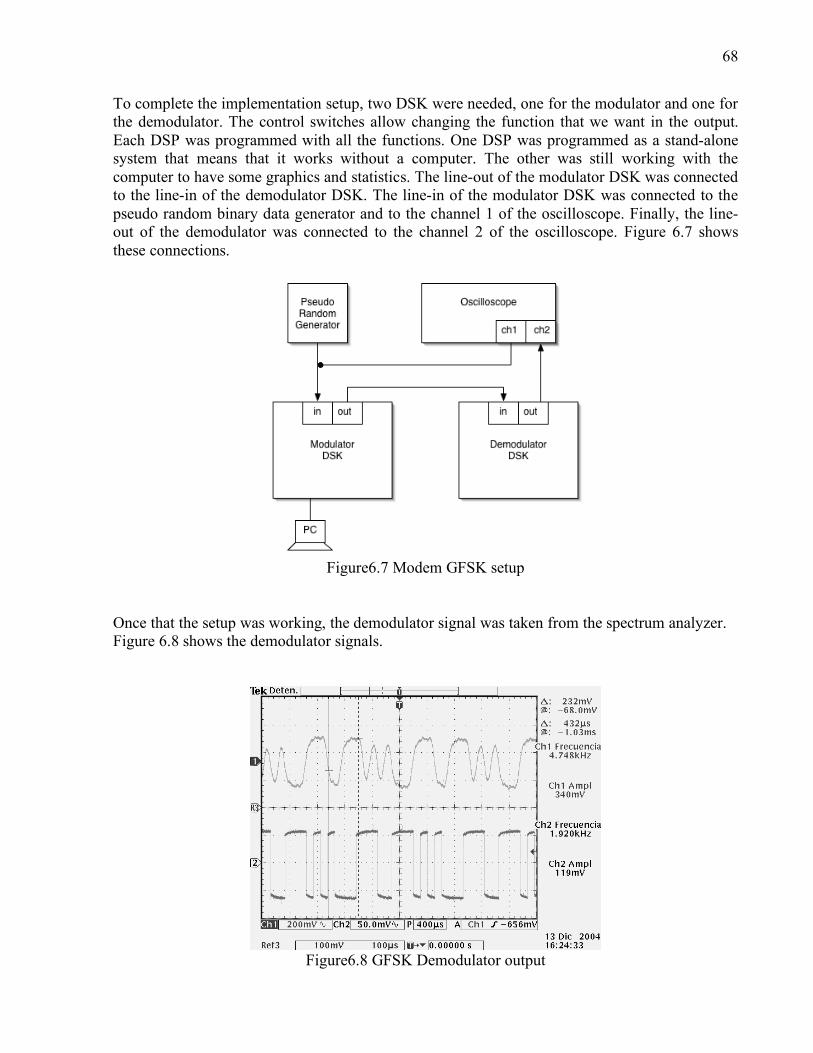
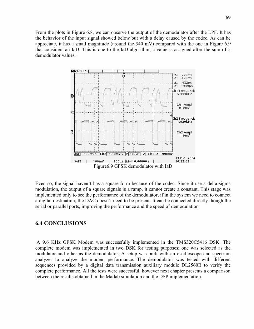
6.3 DEMODULATOR 67
6.4 CONCLUSIONS 69
6.5 BIBLIOGRAPHY 70
7. CONCLUSIONS AND RESULTS 71
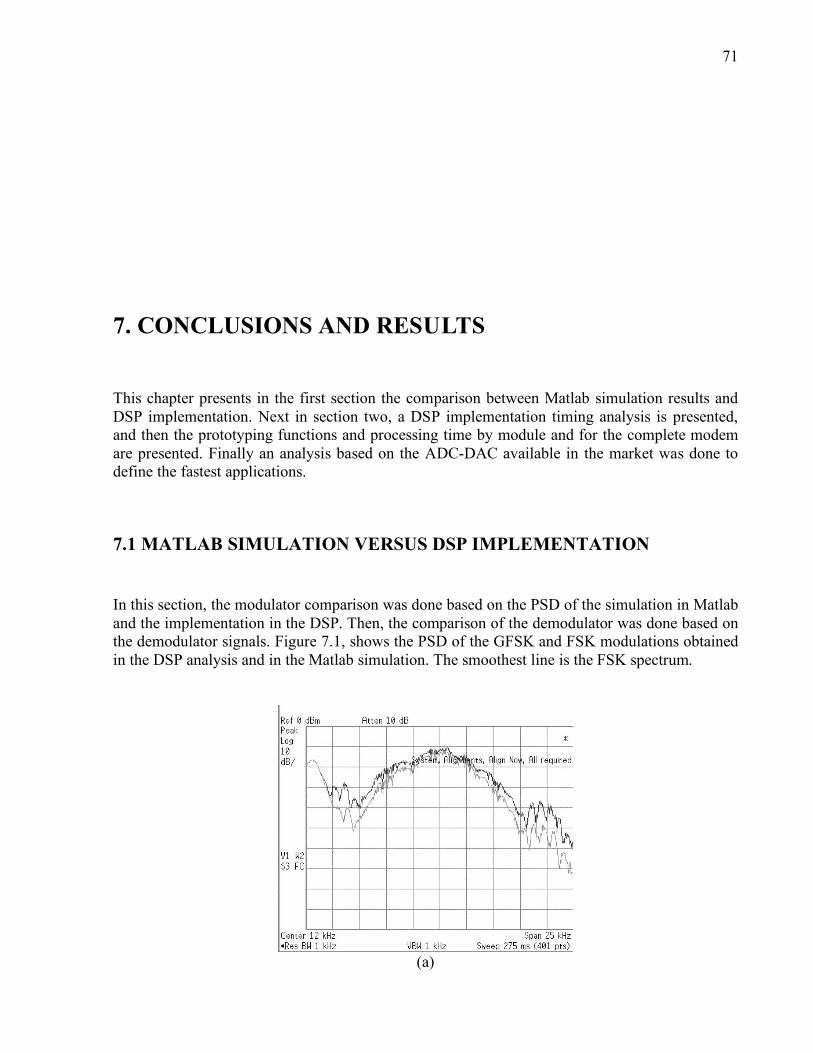
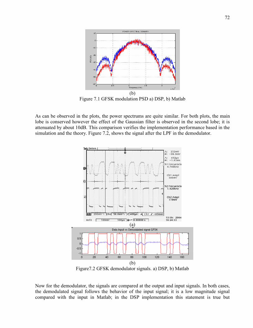
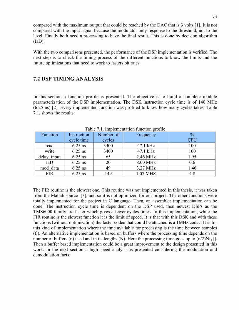
7.1 MATLAB SIMULATION VERSUS DSP IMPLEMENTATION 71
7.2 DSP TIMING ANALYSIS 73
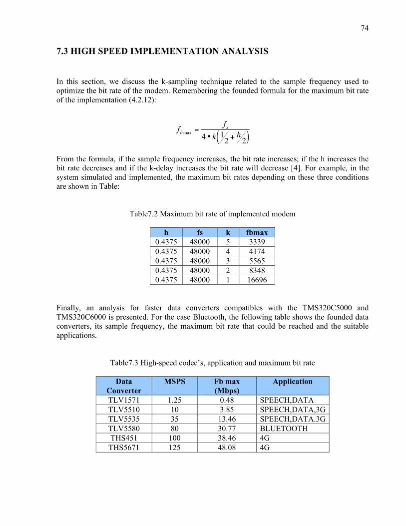
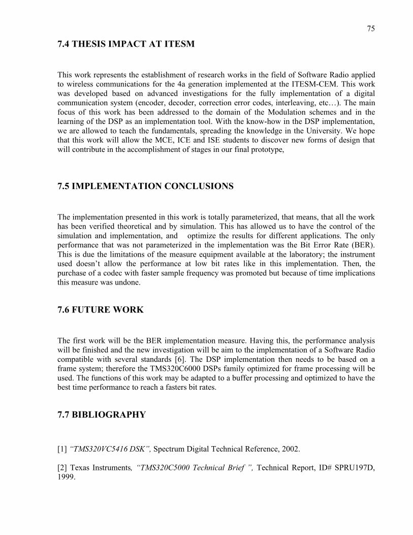
7.3 HIGH SPEED IMPLEMENTATION ANALYSIS 74
7.4 THESIS IMPACT AT ITESM 75
7.5 IMPLEMENTATION CONCLUSIONS 75
7.6 FUTURE WORK 75
7.7 BIBLIOGRAPHY 75
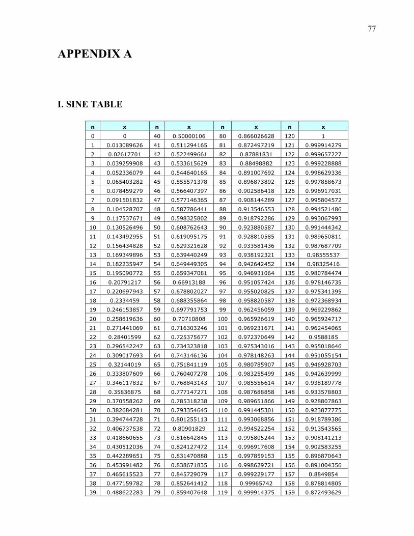
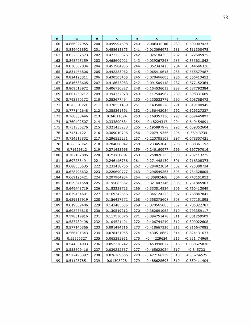
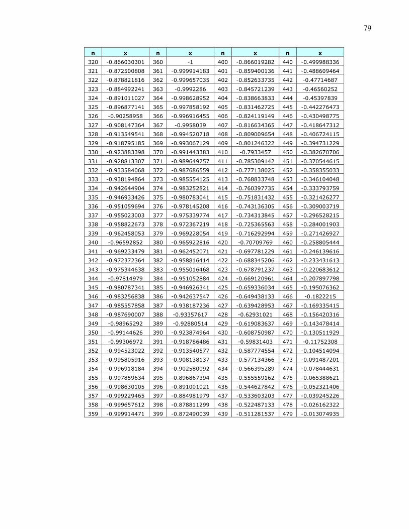
APPENDIX A 77
I. SINE TABLE 77
II. MATLAB MODULATOR FUNCTION 80
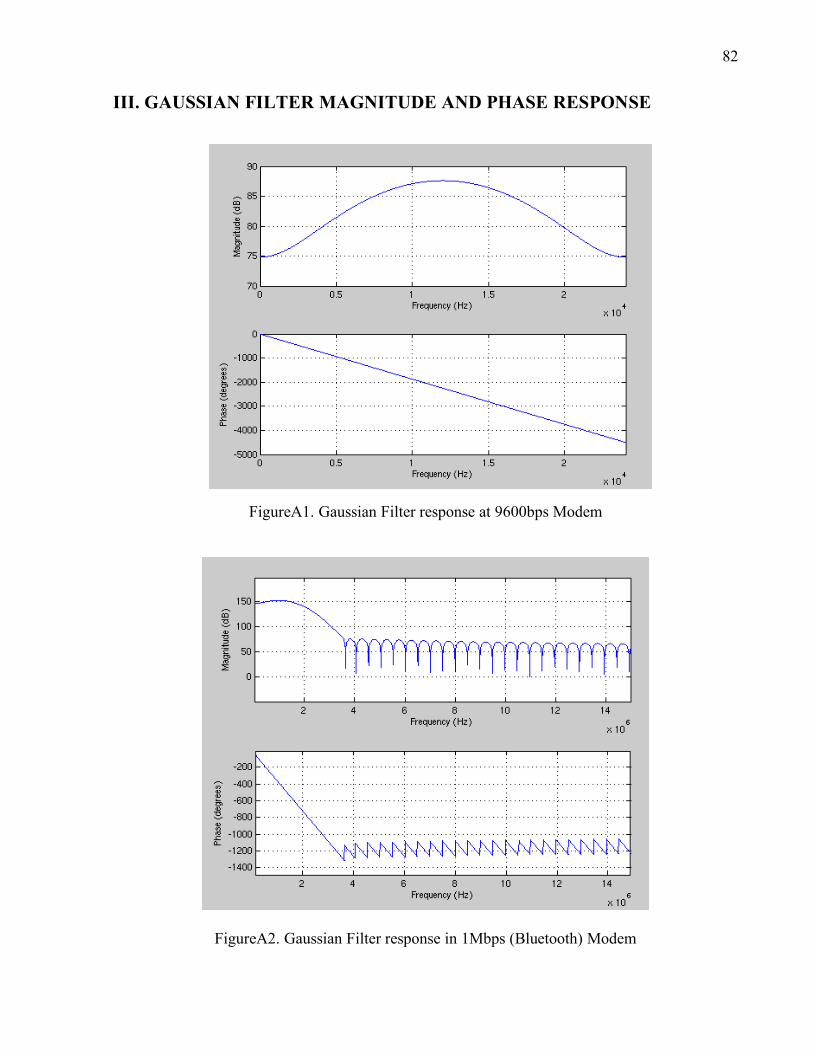
III. GAUSSIAN FILTER MAGNITUDE AND PHASE RESPONSE 82
IV. MATLAB DEMODULATOR FUNCTION 83
APPENDIX B 86
I. MODEM MAIN FUNCTION 86
II. MODULATOR (MOD_DATA) 92
8 III. DEMODULATOR (DELAY_INPUT) 93
IV. INCLUDED FILES 94 A. SINE TABLE 94 B. GAUSSIAN FILTER COEFFICIENTS (MODULATOR) 96 C. LOW PASS FILTER COEFFICIENTS (DEMODULATOR) 96
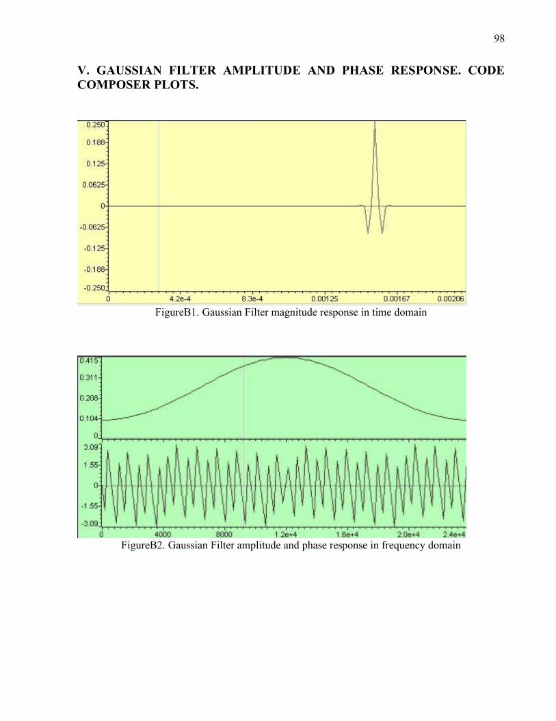
V. GAUSSIAN FILTER AMPLITUDE AND PHASE RESPONSE. CODE COMPOSER PLOTS. 98
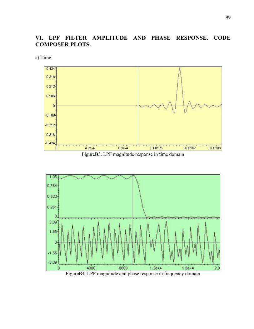
VI. LPF FILTER AMPLITUDE AND PHASE RESPONSE. CODE COMPOSER PLOTS. 99
9
LIST OF FIGURES
Figure2.1 General wireless communication system 15 Figure2.2 General Modulator 16 Figure2.3 BPSK signals 17 Figure2.4 QPSK constellation diagram 18 Figure2.5 π/4-QPSK Constellation diagram 19 Figure2.6 16QAM constellation diagram 20 Figure2.7 FSK signals 21 Figure2.8 MSK signals 22 Figure2.9 Power Spectral Densities of FSK, 16QAM, BPSK and MSK (a) linear (b) logarithmic. 23 Figure2.10 Bandwidth and power efficiency plot 24 Figure3.1 Programmability and specialization comparison of programmable devices 26 Figure3.2 DSPs vendors 28 Figure3.3 TMS320Cx Family of DSP’s 29 Figure3.4 C5000 DSP Platform Roadmap [1] 29 Figure3.5 TMS320C5416 DSK Architecture 30 Figure3.6 PCM3002 architecture 31 Figure3.7 Code Composer Studio development environment [4] 32 Figure4.1 GFSK Modulator 35 Figure4.2 Coherent and Non coherent FSK 35 Figure 4.3 FSK frequencies distribution. 36 Figure4.4 Sine signals for different k, a) k=1, f=1, b) k=5, f=500 Hz, c) k=21, f=2 KHz 37 Figure4.5 FSK continuous phase modulation 38 Figure4.6 Gaussian Filter impulse response 39 Figure4.7 FSK Demodulator 40 Figure4.8 Non-coherent FSK demodulator 40 Figure4.9 Demodulator signals: a) Binary input, b) R(n), c) Rd(n), d) Rt(n) 41 Figure4.10a Demodulator performance with a π/2 delay 42 Figure4.10b Demodulator performance without a π/2 delay 43 Figure4.11 Bit rate (fb) versus sample frequency (fs) 44 Figure4.12 fb and fs behavior 44 Figure 5.1.Frequency frequencies for integer k. 48
10
Figure5.2 Modulation Flow Chart 49 Figure5.3 FSK and GFSK output 50 Figure5.4 FSK and GFSK PSD 51 Figure5.5 FSK and GFSK PSD with higher fs 51 Figure5.6 Demodulator flow chart 52 Figure5.7 a) GFSK demodulated signal and data input, b) GFSK demodulated signal after the
comparator, c) GFSK demodulated signal after IaD 53 Figure5.8 GFSK signals with noise. a) GFSK demodulated signal and data input, b) GFSK
demodulated signal after the comparator, c) GFSK demodulated signal after IaD 54 Figure5.9 GFSK with IaD Probability of error compared with FSK non-coherent demodulation
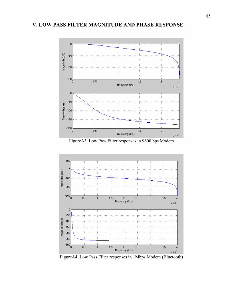
and with FSK coherent demodulation. 55 Figure5.10 Bluetooth GFSK modulation 57 Figure5.11 a) FSK signals b) GFSK signals 58 Figure5.12 GFSK after decision algorithm 59 Figure5.13 BER versus SNR in GFSK modulation 60 Figure6.1 DSP modulator flow chart 64 Figure6.2 GFSK modulation 65 Figure6.3 FSK spectrum 65 Figure6.4 Mirror effect in GFSK modulation 66 Figure6.5 FSK and GFSK spectrum 66 Figure6.6 DSP demodulator Flow chart 67 Figure6.7 Modem GFSK setup 68 Figure6.8 GFSK Demodulator output 68 Figure6.9 GFSK demodulator with IaD 69 Figure 7.1 GFSK modulation PSD a) DSP, b) Matlab 72 Figure7.2 GFSK demodulator signals. a) DSP, b) Matlab 72 FigureA1. Gaussian Filter response at 9600bps Modem 82 FigureA2. Gaussian Filter response in 1Mbps (Bluetooth) Modem 82 FigureA3. Low Pass Filter responses in 9600 bps Modem 85 FigureA4. Low Pass Filter responses in 1Mbps Modem (Bluetooth) 85 FigureB1. Gaussian Filter magnitude response in time domain 98 FigureB2. Gaussian Filter amplitude and phase response in frequency domain 98
11
LIST OF TABLES Table2.1 π/4-DQPSK Phase-change correspondence bits...........................................................19 Table2.2 Modulation Applications .............................................................................................24 Table3.1 Performance, cost, power, flexibility and design complexity comparison of
programmable devices .......................................................................................................27 Table5.1. GFSK parameters with h=0.4375................................................................................48 Table5.2 GFSK parameters with h=0.32 ....................................................................................56 Table6.1 DSP implementation parameters..................................................................................62 Table7.1. Implementation function profile .................................................................................73 Table7.2 Maximum bit rate of implemented modem ..................................................................74 Table7.3 High-speed codec’s, application and maximum bit rate ...............................................74
12
1. INTRODUCTION This Thesis is part of the research work developed for the Mobile Communications Chair of the Electric Department at the ITESM campus Estado de México. The Research work of the Chair concerns the development of 4th Generation Mobile Communications WLAN (Wireless Local Area Network) Systems and Architectures development. The Chair aims to generate specialized human resources in the coding, modulation, radio frequency and integrated circuits related to Mobile Communications. In this Thesis we have focused in the analysis and development of modulation techniques. Modulation techniques as OFDM, QPSK, QAM, GMSK and GFSK among others are used in specific areas of mobile communications as IMT-2000, GSM, GPRS, WCDMA, IEE802.11 and Bluetooth [1]. These modulations combined with multiple access techniques allow having more users and faster systems. In other hand, Software Defined Radios (SDR) perform signal-processing task by running software algorithms on multi-purpose Digital Signal Processors (DSPs). Flexibility offered by DSPs facilitates efficient integration of multiple standards, such as Bluetooth and WLAN, on a single radio system [2]. Then the main goal in this Thesis is the implementation of a wireless Digital Modem under the Bluetooth Standards applied to WPANs over dedicated platforms (Digital Signal Processors platform based).
1.1 MOTIVATION The number of different standards for mobile communication is increasing and thus a need for a universal and flexible transceiver becomes more apparent. Then the need for a programmable transceiver for multiple standards requirements is fundamental and transcendental research. The improvements in digital signal processor (DSP) technology and ADC/DAC technology are undergoing rapid advances [3]. More advantages using software rather than implementing in hardware are the ability to easily upgrade and reuse. A software-defined radio is a radio where the ADC and DAC are performed as close as possible to the antenna. This implies that the demodulation/modulation and signal processing are to be performed by software in the digital domain. This project presents a software radio implementation; it considers the modulation and demodulation stages. The familiarization with the DSP tools, performance and optimization is an important fact in this work thinking in future projects.
13
1.2 OBJECTIVES The objective of this Thesis is to implement a modem in a DSP platform. Gaussian Frequency Shift Keying (GFSK) modulation scheme is the one to be implemented. This modulation is the modulation used in the Bluetooth standard and can be the used to generate other WPANs and WLANs modulation schemes like Gaussian Minimum Shift Keying (GMSK), Phase Shift Keying (PSK) and Quadrature Amplitude Modulation (QAM) [8].
1.3 STATE OF THE ART Demand of future wireless communication services will require an always-on connection according to the Quality of Service QoS and provider service. This QoS involve multiple wireless standards that require intelligent and dynamic portable device. Wireless modems are key part of mobile devices in adequate transmissions according to QoS. In order to adapt different wireless standard, future radios will need to be implemented on software format. Thanks to DSP and wireless technologies, today software modem radios for 2 and 2.5 Generations have already been implemented [3,4]. In other hand, the DSPs implementations have been growing as improves the performance of these. These improvements combined with the development of faster ADC-DAC circuits allow more applications to be implemented. The modulation scheme to be studied, simulated and implemented in this thesis is the Gaussian FSK modulation, used in Bluetooth technology. It is a low-cost, low-power, short-range radio that communicates data and voice in point-to-multipoint networks from 0-10 meters up to 1 Mbps by WPANs [5]. As adoption rates of Bluetooth functionality continues to rise in mobile phones and other devices, it will be essential part in communications of 4G as a devices communications utility. The most significant improve to Bluetooth in this times is the inclusion of Medium Data Rate (MDR) in an updated standard. At present Bluetooth connections run at a relatively modest 720Kb/s, 12 times faster than a modem but over 100 times slower than a LAN connection [6]. The idea is that Bluetooth’s data speed increases two or three orders of magnitude. It will allow most devices connected like notebook PC, personal digital assistant (PDA), cell phone even cars and refrigerator, in a short range.
1.4 ORGANIZATION OF THE THESIS The outline of this Thesis is as follows. After this introduction Chapter 2 present an introduction of a Digital Modulations Schemes used in wireless systems. The chapter presents an overview of the schemes and a bandwidth and power analysis. Chapter 3 describes the main features of the Digital Signal Processors focused in the TMS320C5000 family of Texas Instruments. Chapter 4 presents a theoretical analysis of the GFSK modem. In Chapter 5 a simulation in Matlab is presented based on the theory in Chapter 4. A 9600 bps GFSK modem has been simulated and then a modification for 1Mbps Bluetooth channel. Chapter 6 presents the DSP implementation details of the 9600 bps GFSK modem and finally in Chapter 7 conclusions and results are
14
presented. Appendix A and B present the programs, filters response and sine table of simulation and implementation respectively.
1.5 BIBLIOGRAPHY [1] T. S. Rappaport; “Wireless Communications:Principles and Practices”; Second Edition,
Prentice Hall, 2002. [2] Jeffrey H. Reed, “Software Radio. A modern approach to radio engineering”, Prentice Hall,
USA, 2002. [3] Roel Schiphorst, Fokke Hoeksema, and Kees Slump, “Channel Selection Requirements for
Bluetooth Receivers using a Simple Demodulation Algorithm ”, PRORISC workshop, 29-30 November 2001, Veldhoven, Netherlands, November 2001.
[4] Charles Tibenderana, Stephan Weiss, “A Low-Complexity High-Performance Bluetooth
Receiver”, in Proceedings of IEE Colloquium on DSP enabled Radio, pages pp. 426-435, Livingston, Scotland, Department of Electronics and Computer Science, University of Southampton, UK, 2003.
[5] Kristina Bengtsson, “A DSP based Bluetooth solution, Department of Telecommunications
and Signal Processing”, Master Thesis, Blekinge Institute of Technology. [6] Bluetooth Special Interest Group, “Specification of the Bluetooth System”, February 2002,
Core. [7] Keith E. Nolan, Linda Doyle, “Modulation Scheme Classification for 4G Software Radio
Wireless Networks”, in Proceedings of the IASTED International Conference on Signal Processing, Pattern Recognition, and Applications (SPPRA 2002), June 25-28, 2002, Crete, Greece, pp25-31
[8] Daniel Santana, Javier Gonzalez, “Digital Modulation DSP analysis and implementation
based on integer k-sampling”, in ICED 2004, Internacional Conference on Electronic Design, Veracrúz, Veracrúz, Nov. 21 – 22.
15
2. DIGITAL MODULATIONS SCHEMES APPLIED TO WIRELESS SYSTEMS Digital modulation compared to analog modulation is more robust to noise and interference impairments inherent in wireless channels, more power and spectral efficient modulations, however may be more complex and expensive implementations [1]. This chapter presents a brief review of linear and non-linear digital modulations applied to wireless communications systems, in the first part we study the principal linear and non-linear digital modulations, then in the second part the power and spectral efficiencies are study, and finally in the last part the principal wireless communications systems and modulations are presented. The conclusion at the end of the chapter allows us to present the digital modulation best suited for our application.
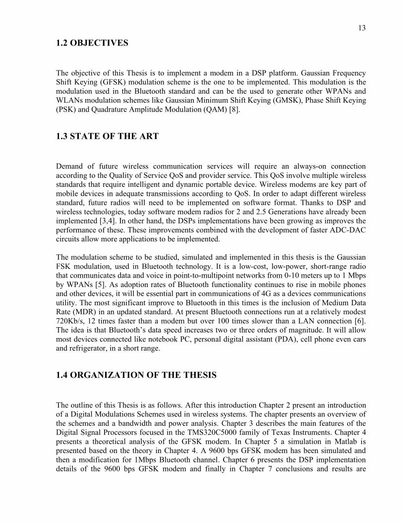
2.1 WIRELESS COMMUNICATION SYSTEM A fundamental wireless communication system involves the information transmission using a wireless channel [2]. Figure 2.1 shows a general wireless communication system.
Figure2.1 General wireless communication system
16
Due to inherent hostile channel characteristics, a wireless system requires multiple signal processing stages as source coding, channel coding, interleaving, band pass modulation and in a spectral limited digital system burst processing. For most of the advanced wireless systems, the air interface and band pass modulation are the more critical and complex stages to implement in the case of software radios, due to spectral efficiency, interferences between wireless systems, etc. For this reason, this work address band pass modulation. Band pass modulation is a process that allows to impresses a digital symbol onto a signal suitable for transmission in a wireless channel. In the case of wireless communication, digital modulation is more suitable that analog modulation due to its noise performance and improved processing techniques. This chapter will allow us to study the digital modulations techniques in order to define best suited for our work. Digital modulation can be regrouped as nonlinear and linear where the first are non-constant envelope in contrast with the last where a constant envelope can be obtained.
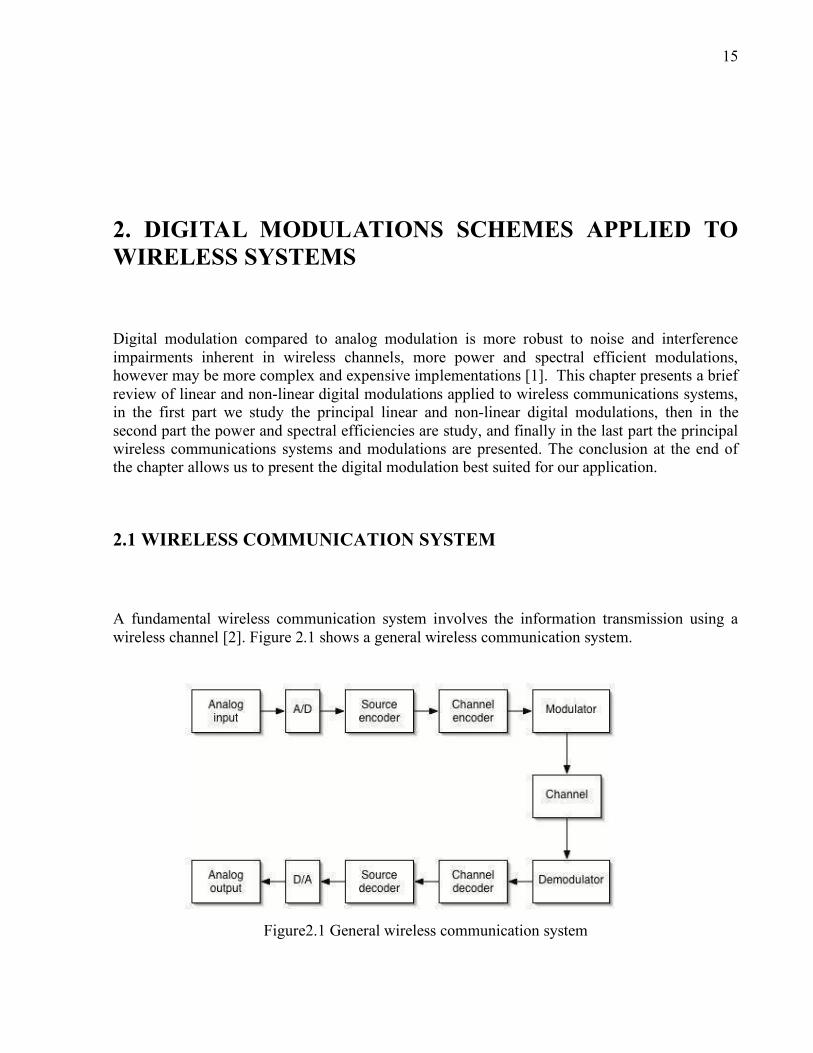
2.2 LINEAR AND NON LINEAR MODULATION TECHNIQUES A general modulator is shown in Figure 2.2. The linearity and non-linearity is depending on the relation between the input and the output of the system [3].
Figure2.2 General Modulator
Linear Modulation:
• The input-output relation of modulator satisfies the “Principle of Superposition” (2.2.1). It is that the output (S) produced by a number of inputs (in) applied simultaneously is equal to the sum of the output that result when the inputs are applied one at a time. If the input is scale by a certain factor, the output of the modulator is scaled by exactly the same factor [4].
S(i
1+ i
2...+ i
n) = S(i
1) + S(i
2)...+ S(i
n) (2.2.1)
!
17
No Linear Modulation:
• Input-Output relation of modulator does not (partially or fully) satisfies the principle of superposition
In other terms, a linear modulation is the one where bits encoded in amplitude (PAM), phase (PSK) or both (MQAM) with no constant envelope. In Nonlinear Modulations, the bits are encoded in frequency (FSK) with constant envelope so they are less susceptible to amplitude and phase nonlinearities introduced by the channel and/or hardware [4]. This chapter shows the Linearity and nonlinearity importance in theoretical and practical aspects. Firstly linear modulations are described, then nonlinear and finally a spectrum analysis of them is shown.
2.3 LINEAR MODULATIONS. PHASE SHIFT KEYING (PSK) The basic kind of Phase Shift Keying (PSK) is the Binary PSK (BPSK) in where binary data are represented by two signals with different phases. Typically these phases are 0 and π, the signals are represented by:
!
s0(t) = Acos2"tfct 0 # t # T for1
s1(t) = $Acos2"tfct 0 # t # T for 0
(2.3.1)
The waveform has a constant envelop and its frequency is constant too. In Figure 2.3 is shown that a "1" causes a phase transition, and a "0" does not produce a transition.
Figure2.3 BPSK signals
2.3.1 QPSK (QUADRATURE PSK)
To increase the bandwidth efficiency of PSK, the MPSK scheme was delivered. In BPSK, a data
18
bit is represented by a symbol, in MPSK, n=log2M data bits are represented, thus the bandwidth
efficiency
!
R
W= log2 M bits /s /Hz[ ] increases n times.
Quadrature PSK (QPSK) is the most often used MPSK (M=4) scheme because it doesn’t suffer from BER degradation while the bandwidth efficiency is increased. So, if we define four signals, each with a phase shift differing by 90O
then we have a quadrature phase shift. The signals are defined by:
!
si(t) = Acos(2"fct + #i), 0 $ t $ T i =1,2,3,4
where
#i =2i %1( )"4
(2.3.2)
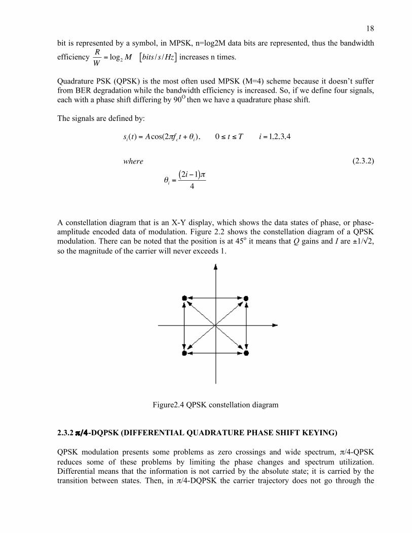
A constellation diagram that is an X-Y display, which shows the data states of phase, or phase-amplitude encoded data of modulation. Figure 2.2 shows the constellation diagram of a QPSK modulation. There can be noted that the position is at 45o it means that Q gains and I are ±1/√2, so the magnitude of the carrier will never exceeds 1.
Figure2.4 QPSK constellation diagram
2.3.2 π /4-DQPSK (DIFFERENTIAL QUADRATURE PHASE SHIFT KEYING) QPSK modulation presents some problems as zero crossings and wide spectrum, π/4-QPSK reduces some of these problems by limiting the phase changes and spectrum utilization. Differential means that the information is not carried by the absolute state; it is carried by the transition between states. Then, in π/4-DQPSK the carrier trajectory does not go through the
19
origin and there can be transition from any symbol position to any other symbol position. The transmitted signal in π/4-DQPSK has the form:
!
x(t) = cos(wct + "(t)) (2.3.3)
Where φ(t) is the phase term that carries the information and it is constant over a symbol period, therefore:
!
x(t) = cos(wct + "k ) for kT # t # (k +1)T (2.3.4)
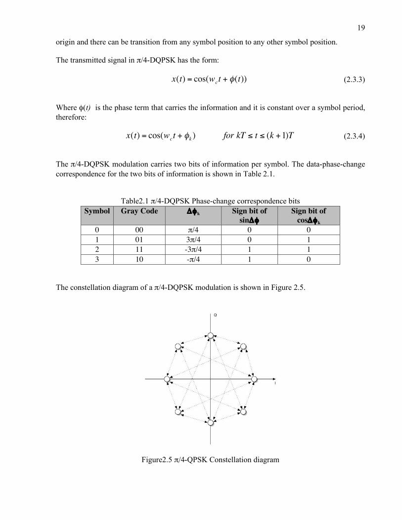
The π/4-DQPSK modulation carries two bits of information per symbol. The data-phase-change correspondence for the two bits of information is shown in Table 2.1.
Table2.1 π/4-DQPSK Phase-change correspondence bits Symbol Gray Code Δφk Sign bit of
The constellation diagram of a π/4-DQPSK modulation is shown in Figure 2.5.
Figure2.5 π/4-QPSK Constellation diagram
20
2.4 LINEAR MODULATIONS. QUADRATURE AMPLITUDE MODULATION (QAM) It is simply a combination of amplitude modulation and phase shift keying. It can be expressed like:
!
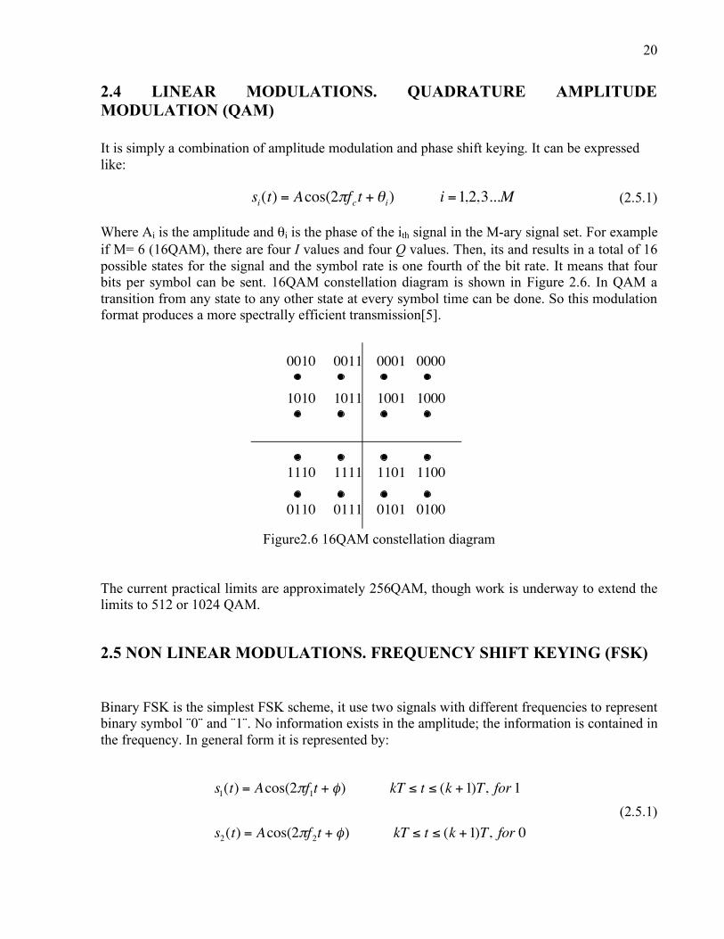
si(t) = Acos(2"fct + #i) i =1,2,3...M (2.5.1) Where Ai is the amplitude and θi is the phase of the ith signal in the M-ary signal set. For example if M= 6 (16QAM), there are four I values and four Q values. Then, its and results in a total of 16 possible states for the signal and the symbol rate is one fourth of the bit rate. It means that four bits per symbol can be sent. 16QAM constellation diagram is shown in Figure 2.6. In QAM a transition from any state to any other state at every symbol time can be done. So this modulation format produces a more spectrally efficient transmission[5].
Figure2.6 16QAM constellation diagram The current practical limits are approximately 256QAM, though work is underway to extend the limits to 512 or 1024 QAM.
2.5 NON LINEAR MODULATIONS. FREQUENCY SHIFT KEYING (FSK) Binary FSK is the simplest FSK scheme, it use two signals with different frequencies to represent binary symbol ¨0¨ and ¨1¨. No information exists in the amplitude; the information is contained in the frequency. In general form it is represented by:
s1(t) = Acos(2"f
1t + #) kT $ t $ (k +1)T, for 1
s2(t) = Acos(2"f
2t + #) kT $ t $ (k +1)T, for 0
(2.5.1)
0010 0011 0001 0000
1010 1011 1001 1000
1110 1111 1101 1100
0110 0111 0101 0100
!
21
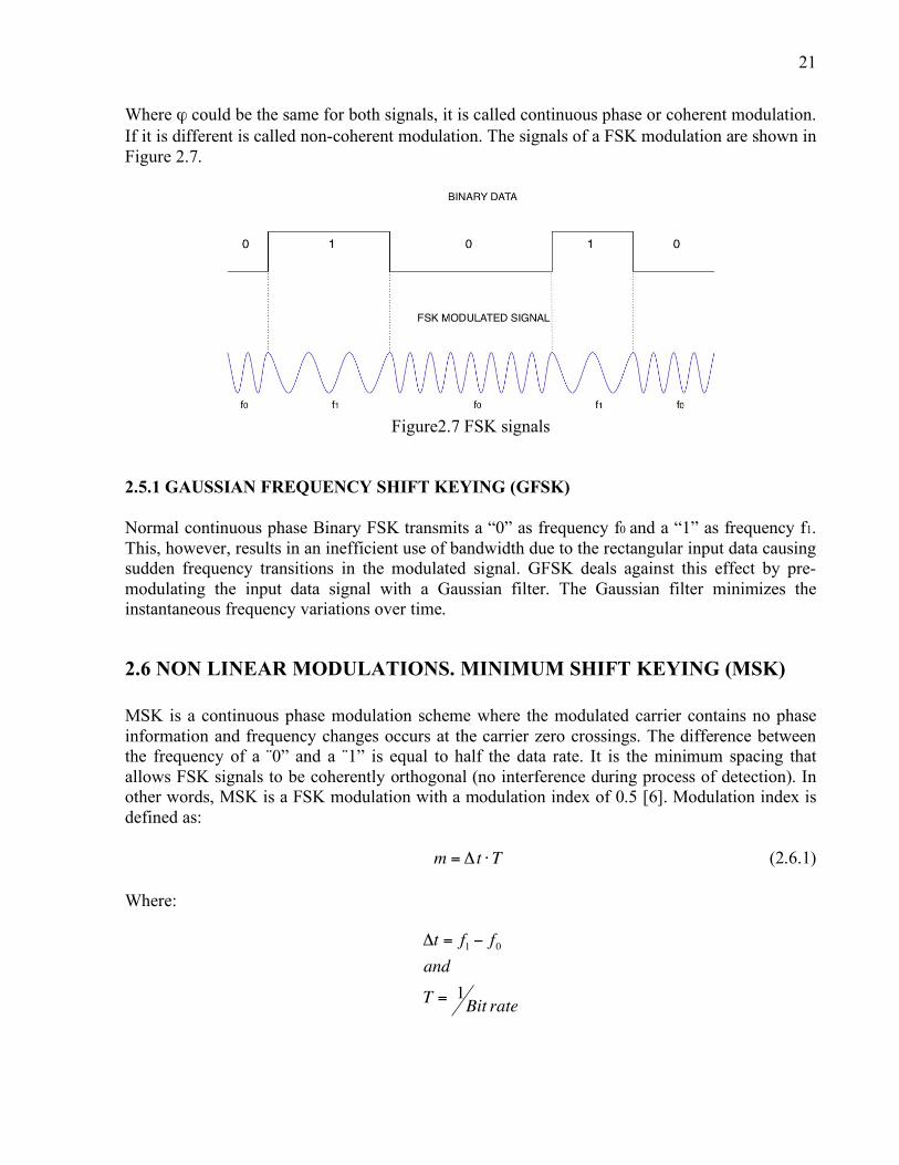
Where ϕ could be the same for both signals, it is called continuous phase or coherent modulation. If it is different is called non-coherent modulation. The signals of a FSK modulation are shown in Figure 2.7.
Figure2.7 FSK signals
2.5.1 GAUSSIAN FREQUENCY SHIFT KEYING (GFSK) Normal continuous phase Binary FSK transmits a “0” as frequency f0 and a “1” as frequency f1. This, however, results in an inefficient use of bandwidth due to the rectangular input data causing sudden frequency transitions in the modulated signal. GFSK deals against this effect by pre-modulating the input data signal with a Gaussian filter. The Gaussian filter minimizes the instantaneous frequency variations over time.
2.6 NON LINEAR MODULATIONS. MINIMUM SHIFT KEYING (MSK) MSK is a continuous phase modulation scheme where the modulated carrier contains no phase information and frequency changes occurs at the carrier zero crossings. The difference between the frequency of a ¨0” and a ¨1” is equal to half the data rate. It is the minimum spacing that allows FSK signals to be coherently orthogonal (no interference during process of detection). In other words, MSK is a FSK modulation with a modulation index of 0.5 [6]. Modulation index is defined as:
!
m = " t #T (2.6.1) Where:
"t = f1# f
0
and
T = 1Bit rate
!
22
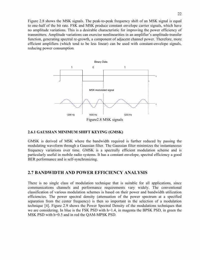
Figure 2.8 shows the MSK signals. The peak-to-peak frequency shift of an MSK signal is equal to one-half of the bit rate. FSK and MSK produce constant envelope carrier signals, which have no amplitude variations. This is a desirable characteristic for improving the power efficiency of transmitters. Amplitude variations can exercise nonlinearities in an amplifier’s amplitude-transfer function, generating spectral re-growth, a component of adjacent channel power. Therefore, more efficient amplifiers (which tend to be less linear) can be used with constant-envelope signals, reducing power consumption.
Figure2.8 MSK signals
2.6.1 GAUSSIAN MINIMUM SHIFT KEYING (GMSK) GMSK is derived of MSK where the bandwidth required is further reduced by passing the modulating waveform through a Gaussian filter. The Gaussian filter minimizes the instantaneous frequency variations over time. GMSK is a spectrally efficient modulation scheme and is particularly useful in mobile radio systems. It has a constant envelope, spectral efficiency a good BER performance and is self-synchronizing.
2.7 BANDWIDTH AND POWER EFFICIENCY ANALYSIS There is no single class of modulation technique that is suitable for all applications, since communications channels and performance requirements vary widely. The conventional classification of various modulation schemes is based on their power and bandwidth utilization efficiencies. The power spectral density (attenuation of the power spectrum at a specified separation from the center frequency) is then so important in the selection of a modulation technique [4]. Figure 2.9 shows the Power Spectral Density of the modulations techniques that we are considering. In blue is the FSK PSD with h=1.4, in magenta the BPSK PSD, in green the MSK PSD with h=0.5 and in red the QAM-MPSK PSD.
23
(a)
(b)
Figure2.9 Power Spectral Densities of FSK, 16QAM, BPSK and MSK (a) linear (b) logarithmic.
We can see that the FSK modulation is the most bandwidth inefficient but the simplest to detect. MSK is a FSK variation with h=0.5 and it is more bandwidth efficient than BPSK but no than QAM. The second plot shows the nodules of the modulated signal. Because 16QAM uses more symbols it the one with the shortest nodules. With these plots is difficult to see the power efficiency then Figure 2.10 presents an analysis based on the bandwidth and the power efficiency.
24
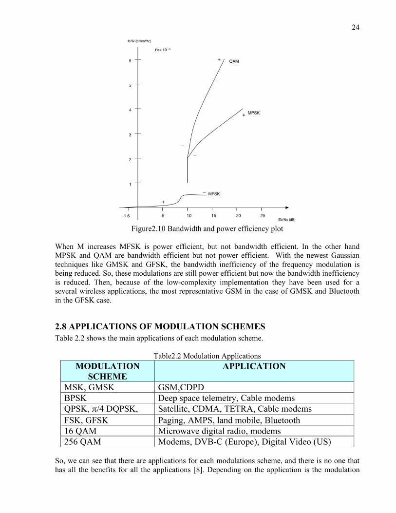
Figure2.10 Bandwidth and power efficiency plot
When M increases MFSK is power efficient, but not bandwidth efficient. In the other hand MPSK and QAM are bandwidth efficient but not power efficient. With the newest Gaussian techniques like GMSK and GFSK, the bandwidth inefficiency of the frequency modulation is being reduced. So, these modulations are still power efficient but now the bandwidth inefficiency is reduced. Then, because of the low-complexity implementation they have been used for a several wireless applications, the most representative GSM in the case of GMSK and Bluetooth in the GFSK case.
2.8 APPLICATIONS OF MODULATION SCHEMES Table 2.2 shows the main applications of each modulation scheme.
Table2.2 Modulation Applications MODULATION
SCHEME APPLICATION
MSK, GMSK GSM,CDPD BPSK Deep space telemetry, Cable modems QPSK, π/4 DQPSK, Satellite, CDMA, TETRA, Cable modems FSK, GFSK Paging, AMPS, land mobile, Bluetooth 16 QAM Microwave digital radio, modems 256 QAM Modems, DVB-C (Europe), Digital Video (US)
So, we can see that there are applications for each modulations scheme, and there is no one that has all the benefits for all the applications [8]. Depending on the application is the modulation
25
scheme that is selected, in the terms of the bandwidth and power limitations, and complexity of implementation (that is reflected in cost). That’s why the PSK and QAM modulations are used mainly in the bandwidth-limited systems, the FSK in the power limited systems.
2.9 CONCLUSIONS Because the power efficiency and the low-complexity demodulation implementation, FSK modulation was selected to the first implementation. Having a FSK implementation is easily the transition to a MSK and a binary PSK. In other hand, a Gaussian Filter implementation is considered too. Having it, GFSK and GMSK could be generated. It could guide us throw the future implementation of a multiple standards Software Radio. In this work we will be focused in a GFSK modulator and demodulator implementation based on the Bluetooth norm that is being developing for a short-range wireless communications. Bluetooth uses Gaussian frequency shift keying (GFSK) with a modulation index between 0.28 and 0.35. In the next chapters the simulation and implementation will be shown.
2.10 BIBLIOGRAPHY [1] Fuqin Xiong, “Digital Modulation Techniques”, Artech House, USA, 2000. [2] T. S. Rappaport; “Wireless Communications”; Prentice Hall, 2002. [3] Ambreen Ali, Felicia Berlanga “Linear vs Constant Envelope Modulation Schemes in
Wireless Communication Systems”, Report, University of Texas in Dallas. [4] Dr. Mike Fitton, “Telecommunications Research Lab”, Report, Toshiba Research Europe Limited. [5] Leon W. Couch II, “Modern Communication Systems. Principles and Applications”, Prentice
Hall, 1995. [6] HP application note 1298, “Digital Modulation in Communications Systems- An
Introduction”, USA, 1997. [7] Kevin C. Yu, Andrea J. Goldsmith, “Linear Models and Capacity Bounds for Continuous
Phase Modulation”, in IEEE International Conference on Communications, pp. 722-726, April 2002.
[8] Geoff Smithson, “Introduction to Digital Modulation Schemes”, IEE Colloquium on The
Design of Digital Cellular Handsets, London , UK, page(s): 2.1-2.9, 4 Mar 1998.
26
3. DIGITAL SIGNAL PROCESSORS In this chapter a brief introduction to digital signal processors DSP is provided. DSPs are digital programmable device well suited for communication applications. As DSPs, ASICs and FPGAs are also programmable devices that can be used to implement digital functions. After this introduction, a brief comparison between these devices is provided, then a description of different DSP and components, the tools to program the DSP and finally the description of the DSP used in this project.
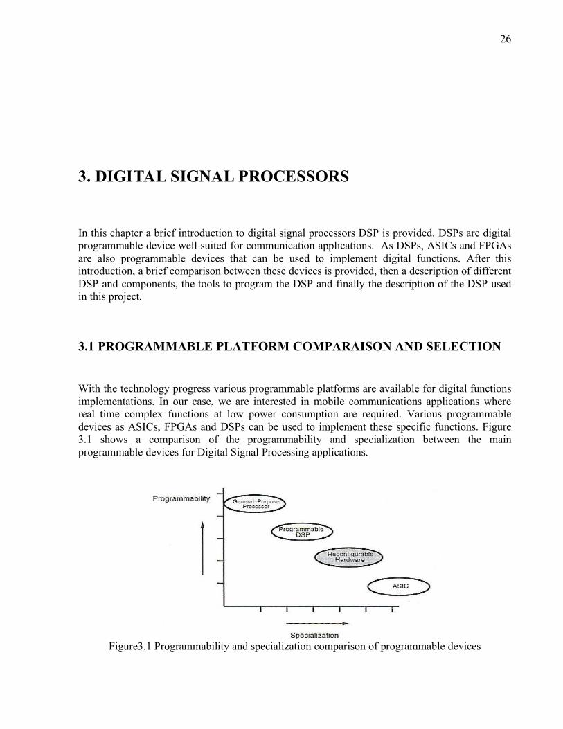
3.1 PROGRAMMABLE PLATFORM COMPARAISON AND SELECTION With the technology progress various programmable platforms are available for digital functions implementations. In our case, we are interested in mobile communications applications where real time complex functions at low power consumption are required. Various programmable devices as ASICs, FPGAs and DSPs can be used to implement these specific functions. Figure 3.1 shows a comparison of the programmability and specialization between the main programmable devices for Digital Signal Processing applications.
Figure3.1 Programmability and specialization comparison of programmable devices
27
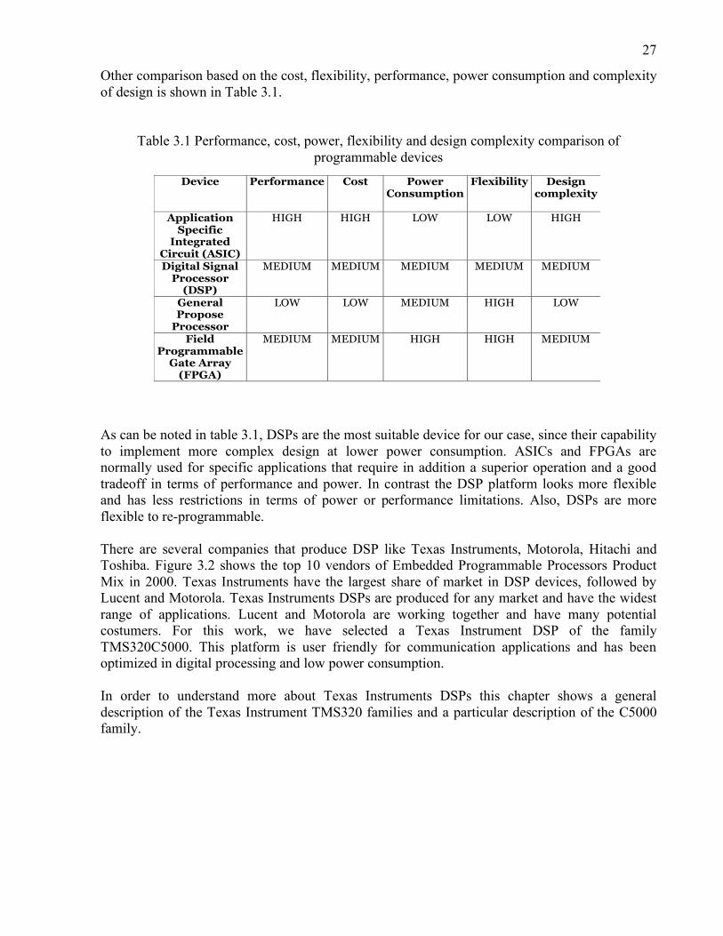
Other comparison based on the cost, flexibility, performance, power consumption and complexity of design is shown in Table 3.1.
Table 3.1 Performance, cost, power, flexibility and design complexity comparison of programmable devices
As can be noted in table 3.1, DSPs are the most suitable device for our case, since their capability to implement more complex design at lower power consumption. ASICs and FPGAs are normally used for specific applications that require in addition a superior operation and a good tradeoff in terms of performance and power. In contrast the DSP platform looks more flexible and has less restrictions in terms of power or performance limitations. Also, DSPs are more flexible to re-programmable. There are several companies that produce DSP like Texas Instruments, Motorola, Hitachi and Toshiba. Figure 3.2 shows the top 10 vendors of Embedded Programmable Processors Product Mix in 2000. Texas Instruments have the largest share of market in DSP devices, followed by Lucent and Motorola. Texas Instruments DSPs are produced for any market and have the widest range of applications. Lucent and Motorola are working together and have many potential costumers. For this work, we have selected a Texas Instrument DSP of the family TMS320C5000. This platform is user friendly for communication applications and has been optimized in digital processing and low power consumption. In order to understand more about Texas Instruments DSPs this chapter shows a general description of the Texas Instrument TMS320 families and a particular description of the C5000 family.
Device Performance Cost PowerConsumption
Flexibility Designcomplexity
ApplicationSpecific
IntegratedCircuit (ASIC)
HIGH HIGH LOW LOW HIGH
Digital SignalProcessor
(DSP)
MEDIUM MEDIUM MEDIUM MEDIUM MEDIUM
GeneralPropose
Processor
LOW LOW MEDIUM HIGH LOW
FieldProgrammable
Gate Array(FPGA)
MEDIUM MEDIUM HIGH HIGH MEDIUM
28
Figure3.2 DSPs vendors
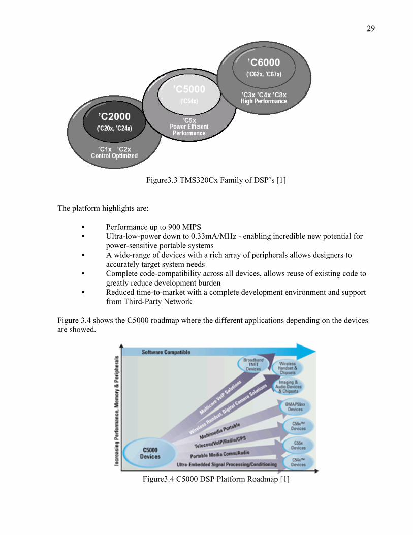
3.2 TEXAS INSTRUMENT TMS320CX DIGITAL SIGNAL PROCESSORS FAMILY Each generation of TMS320Cx devices uses a core central processing unit (CPU) that is combined with a variety of on-chip memory and peripheral configurations. These various configurations satisfy a wide range of needs in the worldwide electronics market. When memory and peripherals are integrated with a CPU into one chip, the overall system cost is greatly reduced, and circuit board space is reduced. Texas Instruments have been developing three important families of Digital Signal Processors: The TMS320C2x family oriented to control applications, the TMS320C5000 family oriented to power efficient performance and the TMS320C6000 oriented to a high performance. Figure 3.3 shows the progression of the TMS320Cx devices. With power consumption as low as 0.45 mA/MHz and performance up to 600 MIPS, the C5000 DSP platform is optimized for portable media and communication products like digital music players, GPS receivers, portable medical equipment, feature phones, modems, 3G cell phones, and portable imaging.
29
Figure3.3 TMS320Cx Family of DSP’s [1]
The platform highlights are: ▪ Performance up to 900 MIPS
▪ Ultra-low-power down to 0.33mA/MHz - enabling incredible new potential for power-sensitive portable systems
▪ A wide-range of devices with a rich array of peripherals allows designers to accurately target system needs
▪ Complete code-compatibility across all devices, allows reuse of existing code to greatly reduce development burden
▪ Reduced time-to-market with a complete development environment and support from Third-Party Network
Figure 3.4 shows the C5000 roadmap where the different applications depending on the devices are showed.
Figure3.4 C5000 DSP Platform Roadmap [1]
30
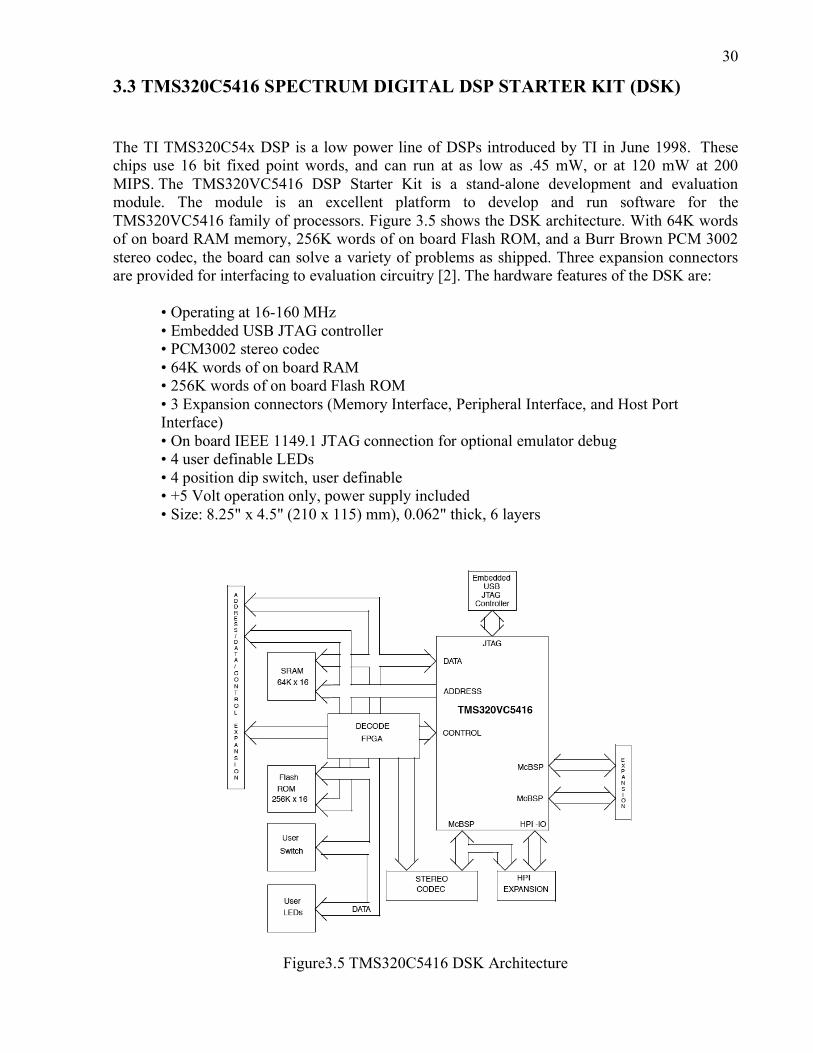
3.3 TMS320C5416 SPECTRUM DIGITAL DSP STARTER KIT (DSK) The TI TMS320C54x DSP is a low power line of DSPs introduced by TI in June 1998. These chips use 16 bit fixed point words, and can run at as low as .45 mW, or at 120 mW at 200 MIPS. The TMS320VC5416 DSP Starter Kit is a stand-alone development and evaluation module. The module is an excellent platform to develop and run software for the TMS320VC5416 family of processors. Figure 3.5 shows the DSK architecture. With 64K words of on board RAM memory, 256K words of on board Flash ROM, and a Burr Brown PCM 3002 stereo codec, the board can solve a variety of problems as shipped. Three expansion connectors are provided for interfacing to evaluation circuitry [2]. The hardware features of the DSK are: • Operating at 16-160 MHz
• Embedded USB JTAG controller • PCM3002 stereo codec • 64K words of on board RAM • 256K words of on board Flash ROM
• 3 Expansion connectors (Memory Interface, Peripheral Interface, and Host Port Interface)
• On board IEEE 1149.1 JTAG connection for optional emulator debug • 4 user definable LEDs • 4 position dip switch, user definable • +5 Volt operation only, power supply included • Size: 8.25" x 4.5" (210 x 115) mm), 0.062" thick, 6 layers
Figure3.5 TMS320C5416 DSK Architecture
31
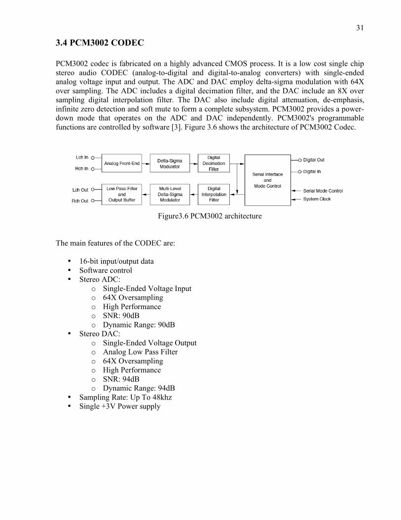
3.4 PCM3002 CODEC PCM3002 codec is fabricated on a highly advanced CMOS process. It is a low cost single chip stereo audio CODEC (analog-to-digital and digital-to-analog converters) with single-ended analog voltage input and output. The ADC and DAC employ delta-sigma modulation with 64X over sampling. The ADC includes a digital decimation filter, and the DAC include an 8X over sampling digital interpolation filter. The DAC also include digital attenuation, de-emphasis, infinite zero detection and soft mute to form a complete subsystem. PCM3002 provides a power-down mode that operates on the ADC and DAC independently. PCM3002's programmable functions are controlled by software [3]. Figure 3.6 shows the architecture of PCM3002 Codec.
Figure3.6 PCM3002 architecture
The main features of the CODEC are:
• 16-bit input/output data • Software control • Stereo ADC:
o Single-Ended Voltage Input o 64X Oversampling o High Performance o SNR: 90dB o Dynamic Range: 90dB
• Stereo DAC: o Single-Ended Voltage Output o Analog Low Pass Filter o 64X Oversampling o High Performance o SNR: 94dB o Dynamic Range: 94dB
• Sampling Rate: Up To 48khz • Single +3V Power supply
32
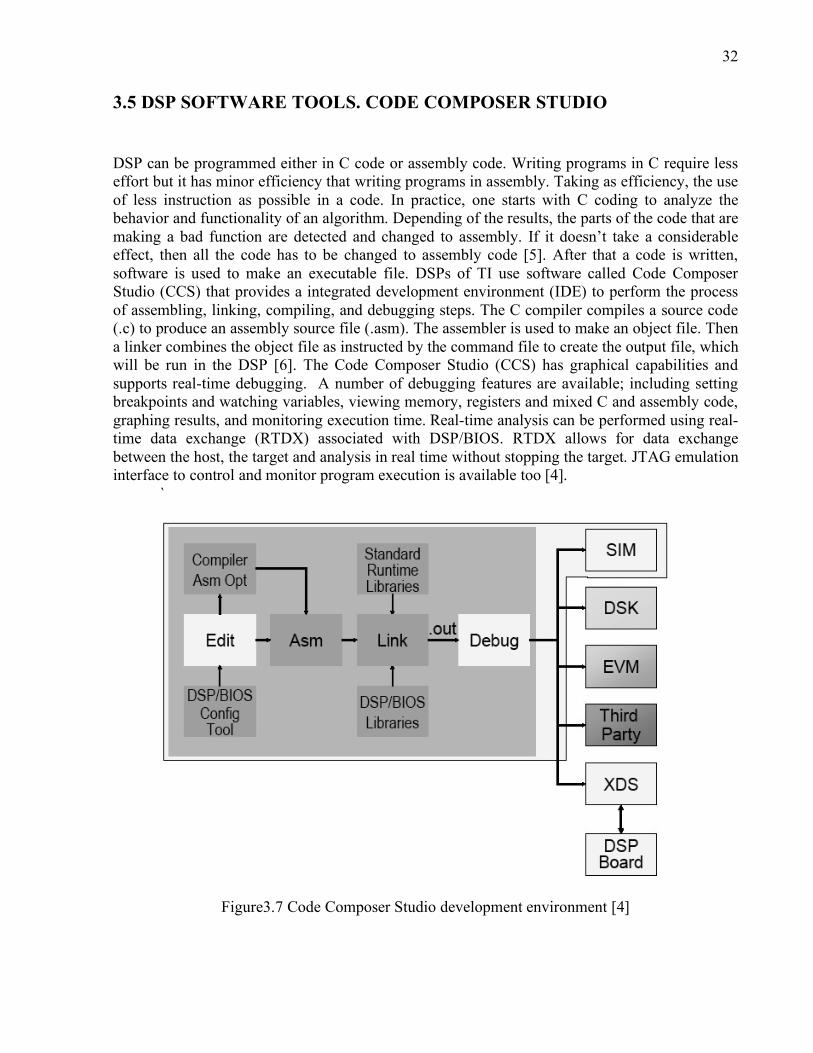
3.5 DSP SOFTWARE TOOLS. CODE COMPOSER STUDIO DSP can be programmed either in C code or assembly code. Writing programs in C require less effort but it has minor efficiency that writing programs in assembly. Taking as efficiency, the use of less instruction as possible in a code. In practice, one starts with C coding to analyze the behavior and functionality of an algorithm. Depending of the results, the parts of the code that are making a bad function are detected and changed to assembly. If it doesn’t take a considerable effect, then all the code has to be changed to assembly code [5]. After that a code is written, software is used to make an executable file. DSPs of TI use software called Code Composer Studio (CCS) that provides a integrated development environment (IDE) to perform the process of assembling, linking, compiling, and debugging steps. The C compiler compiles a source code (.c) to produce an assembly source file (.asm). The assembler is used to make an object file. Then a linker combines the object file as instructed by the command file to create the output file, which will be run in the DSP [6]. The Code Composer Studio (CCS) has graphical capabilities and supports real-time debugging. A number of debugging features are available; including setting breakpoints and watching variables, viewing memory, registers and mixed C and assembly code, graphing results, and monitoring execution time. Real-time analysis can be performed using real-time data exchange (RTDX) associated with DSP/BIOS. RTDX allows for data exchange between the host, the target and analysis in real time without stopping the target. JTAG emulation interface to control and monitor program execution is available too [4].
`
Figure3.7 Code Composer Studio development environment [4]
33
DSP/BIOS, is a configuration tool used in Code Composer to generate code to configure pheriphericals, memory, interrupst, timers and almost all the DSK features. It is an alternative form to program the DSK features but in a more effortless way.
3.6 CONCLUSIONS In this chapter we have presented a brief description of DSP, then a comparison with other programmable platforms as ASIC and FPGA in order to evaluate the suitability of DSP for our applications. Once the DSP platform has been selected, the characteristics of the implementations tools for the specific platform have been presented. The TMS320C5000 family was selected for our implementation, then the TMS320C5416 DSK has been used as a stand-alone development and evaluation module. Based in this DSK, we have developed a series of programs for the TMS320C5416 family, these programs can be simulated as hardware and software using the Code Composer Studio and the PCM 3002 CODEC.
ID#spru328B, 2000. [5] Nasser Kehtarnavaz, Mansour Keramat, “DSP System Design: Using the TMS3320C6000”,
Prentice Hall, New Jersey, 2001. [6] Rulph Chassaing, “DSP Applications Using C and TMS320C6x DSK”, John Wiley and Sons,
USA, 2002.
34
4. GFSK MODEM ANALYSIS In this chapter a Gaussian Frequency Shift Key Modem DSP implemented is presented. As was presented in previous chapters, a GFSK modulation has been selected due to its power-efficient modulation, simplicity to be implement on digital programmable platforms, robustness to wireless channels impairments, low power consumption implementation and ability to be translated to other modulation schemes. GFSK modulation is used in Bluetooth standard for short-distance digital radio connections. Bluetooth standard has been designed to implement robust and low complex wireless communication networks. Low power and low cost are also two major key points for Bluetooth. The Bluetooth standard operates in the ISM (Industrial Scientific and Medical) band, at 2.4 GHz [1]. This is one of free license frequency band available worldwide. The frequency bands may be different from country to country, regarding location and width. In most of Europe and the USA the frequency band lies between 2400 and 2483.5 MHz. The modulation format in the Bluetooth standard is Gaussian-shaped binary frequency shift keying, GFSK, with a BT (Bandwidth, Symbol period) product equal to 0.5 [2]. The data symbol rate is 1 MSymbol/s. The purpose of a binary modulation scheme is to achieve a robust format. This also makes the transceiver less complex and thereby the cost is reduced. The demodulation can simply be done using a non-coherent frequency demodulation. Phase and amplitude are not of importance. After this introduction and once the modulation and DSP platform have been chosen, the theoretical analysis of the GFSK modulation and demodulation will be presented in this chapter. In first place the modulator analysis is presented then the demodulator analysis.
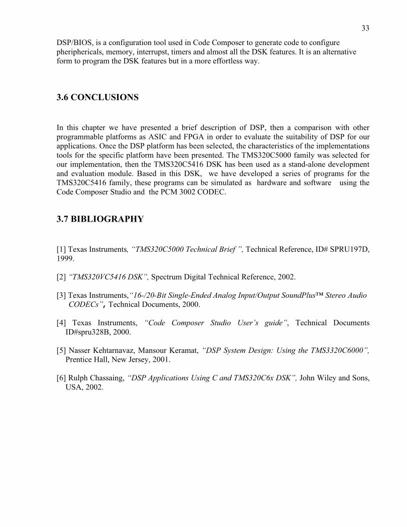
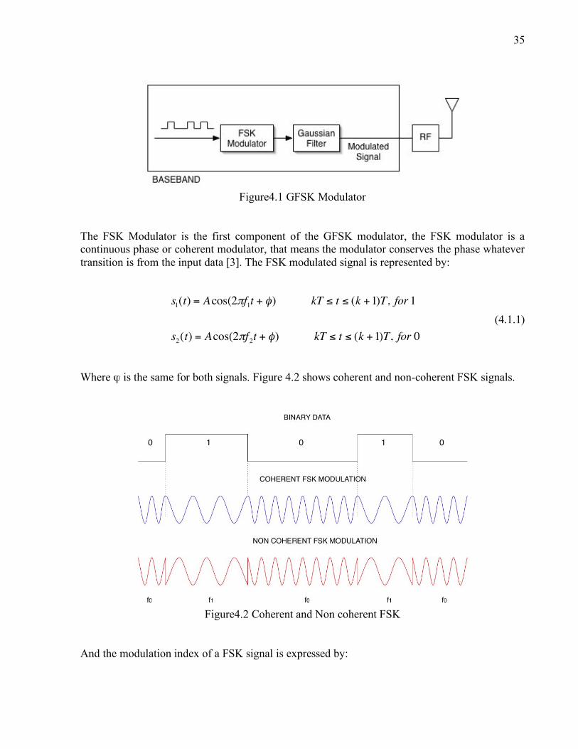
4.1 GFSK MODULATOR In a wireless GFSK Modulator, the binary data are converted to a non-return to zero (NRZ) format where a 1 represents a binary ¨1¨ and a binary ¨0¨ is represented by a -1. Then the data are modulated by a FSK modulator and filtered by a Gaussian Filter. Finally, in wireless applications, the modulated signal enters to the RF section to be transmitted through the air. Figure 4.1 shows a block diagram of GFSK modulator.
35
Figure4.1 GFSK Modulator
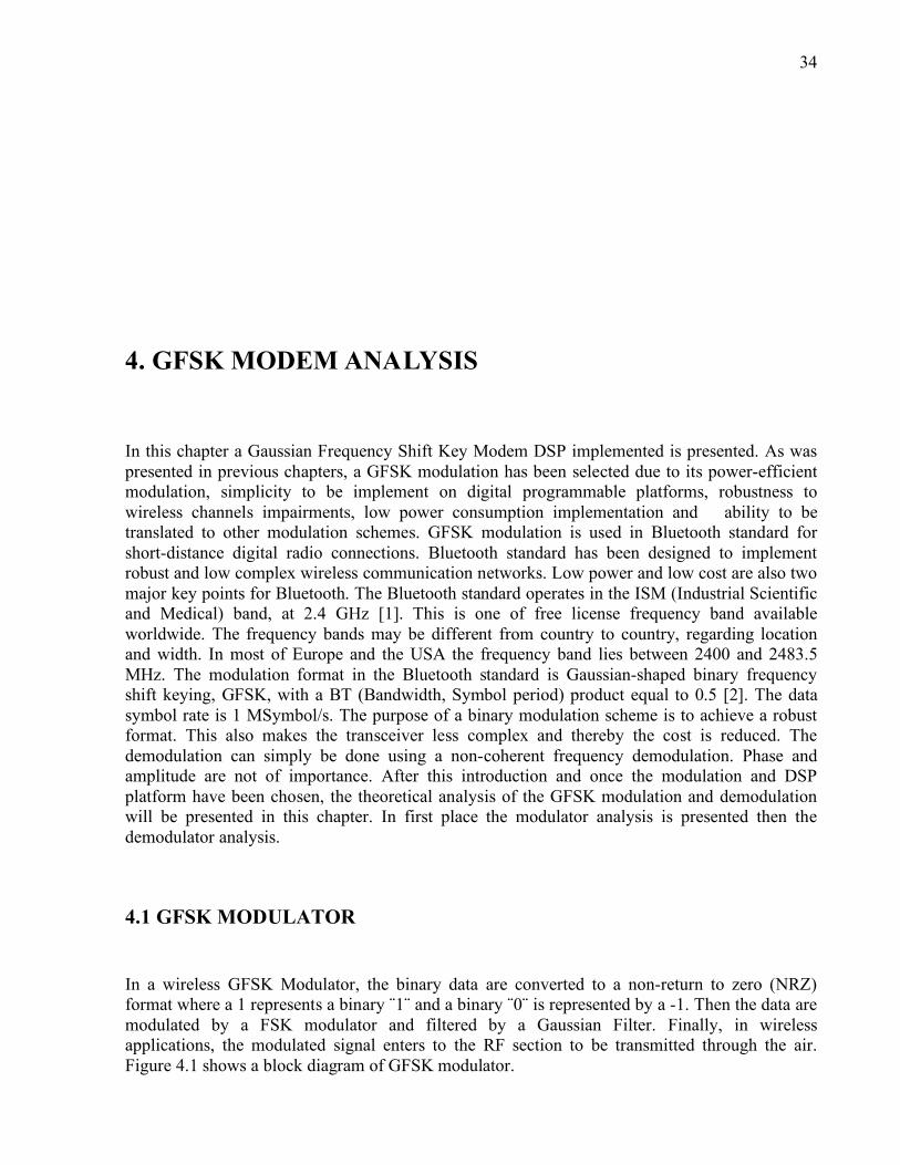
The FSK Modulator is the first component of the GFSK modulator, the FSK modulator is a continuous phase or coherent modulator, that means the modulator conserves the phase whatever transition is from the input data [3]. The FSK modulated signal is represented by:
!
s1(t) = Acos(2"f
1t + #) kT $ t $ (k +1)T, for 1
s2(t) = Acos(2"f
2t + #) kT $ t $ (k +1)T, for 0
(4.1.1)
Where ϕ is the same for both signals. Figure 4.2 shows coherent and non-coherent FSK signals.
Figure4.2 Coherent and Non coherent FSK
And the modulation index of a FSK signal is expressed by:
36
!
h ="f
fb (4.1.2)
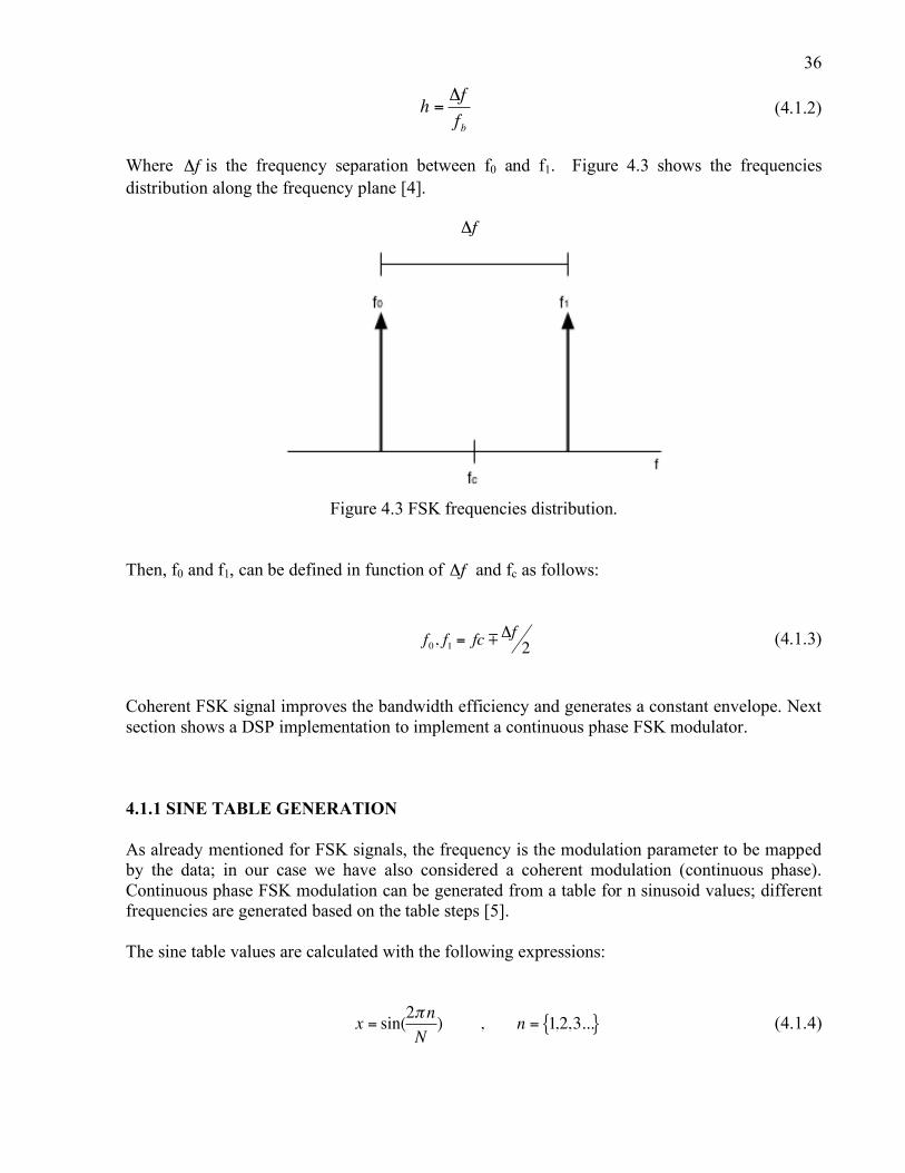
Where
!
"f is the frequency separation between f0 and f1. Figure 4.3 shows the frequencies distribution along the frequency plane [4].
!
"f
Figure 4.3 FSK frequencies distribution.
Then, f0 and f1, can be defined in function of
!
"f and fc as follows:
!
f0, f1
= fc m"f2
(4.1.3) Coherent FSK signal improves the bandwidth efficiency and generates a constant envelope. Next section shows a DSP implementation to implement a continuous phase FSK modulator. 4.1.1 SINE TABLE GENERATION As already mentioned for FSK signals, the frequency is the modulation parameter to be mapped by the data; in our case we have also considered a coherent modulation (continuous phase). Continuous phase FSK modulation can be generated from a table for n sinusoid values; different frequencies are generated based on the table steps [5]. The sine table values are calculated with the following expressions:
x = sin(2" n
N) , n = 1,2,3...{ } (4.1.4)
!
37
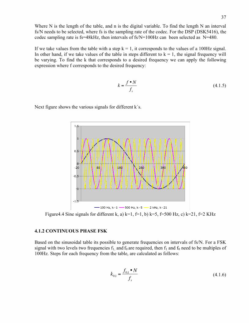
Where N is the length of the table, and n is the digital variable. To find the length N an interval fs/N needs to be selected, where fs is the sampling rate of the codec. For the DSP (DSK5416), the codec sampling rate is fs=48kHz, then intervals of fs/N=100Hz can been selected as N=480. If we take values from the table with a step k = 1, it corresponds to the values of a 100Hz signal. In other hand, if we take values of the table in steps different to k = 1, the signal frequency will be varying. To find the k that corresponds to a desired frequency we can apply the following expression where f corresponds to the desired frequency:
!
k =f •N
fs (4.1.5)
Next figure shows the various signals for different k´s.
Figure4.4 Sine signals for different k, a) k=1, f=1, b) k=5, f=500 Hz, c) k=21, f=2 KHz
4.1.2 CONTINUOUS PHASE FSK Based on the sinusoidal table its possible to generate frequencies on intervals of fs/N. For a FSK signal with two levels two frequencies f1, and f0 are required, then f1 and f0 need to be multiples of 100Hz. Steps for each frequency from the table, are calculated as follows:
k0,1
=f0,1
•N
fs (4.1.6)
!
38
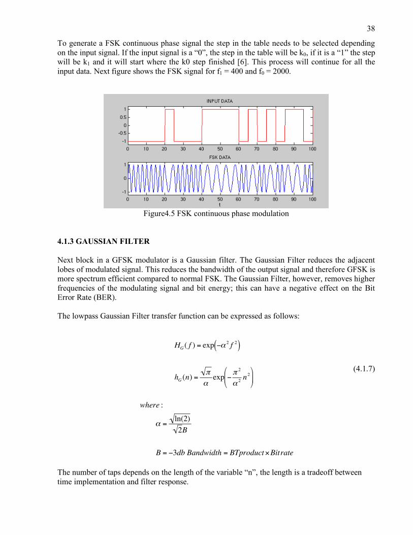
To generate a FSK continuous phase signal the step in the table needs to be selected depending on the input signal. If the input signal is a “0”, the step in the table will be k0, if it is a “1” the step will be k1 and it will start where the k0 step finished [6]. This process will continue for all the input data. Next figure shows the FSK signal for f1 = 400 and f0 = 2000.
Figure4.5 FSK continuous phase modulation
4.1.3 GAUSSIAN FILTER Next block in a GFSK modulator is a Gaussian filter. The Gaussian Filter reduces the adjacent lobes of modulated signal. This reduces the bandwidth of the output signal and therefore GFSK is more spectrum efficient compared to normal FSK. The Gaussian Filter, however, removes higher frequencies of the modulating signal and bit energy; this can have a negative effect on the Bit Error Rate (BER). The lowpass Gaussian Filter transfer function can be expressed as follows:
!
HG ( f ) = exp "# 2f2( )
hG (n) =$
#exp "
$ 2
# 2n2
%
& '
(
) * (4.1.7)
!
where :
" =ln(2)
2B
B = #3db Bandwidth = BTproduct$Bitrate
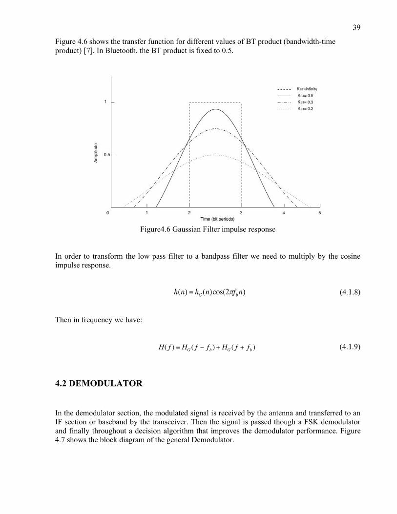
The number of taps depends on the length of the variable “n”, the length is a tradeoff between time implementation and filter response.
39
Figure 4.6 shows the transfer function for different values of BT product (bandwidth-time product) [7]. In Bluetooth, the BT product is fixed to 0.5.
Figure4.6 Gaussian Filter impulse response
In order to transform the low pass filter to a bandpass filter we need to multiply by the cosine impulse response.
!
h(n) = hG (n)cos(2"fbn) (4.1.8) Then in frequency we have:
!
H( f ) = HG ( f " fb ) + HG ( f + fb ) (4.1.9)
4.2 DEMODULATOR In the demodulator section, the modulated signal is received by the antenna and transferred to an IF section or baseband by the transceiver. Then the signal is passed though a FSK demodulator and finally throughout a decision algorithm that improves the demodulator performance. Figure 4.7 shows the block diagram of the general Demodulator.
40
Figure4.7 FSK Demodulator
The demodulator use a non-coherent demodulation, it detects the frequency changes and simplify the DSP implementation. Amplitude and phase are irrelevant in this case. It also reduces complexity and the processing time. The decision algorithm improves the demodulator performance. Next section presents the blocks analysis. 4.2.1 Non-coherent demodulation GFSK demodulator has been implemented using non-coherent Quadrature Detector or FM discriminator showed in Figure 4.8. The goal of this method is to translate a frequency shift into an amplitude change [8]. This is possible by delaying the input signal and multiplying it with the original (not time-delayed).
Figure4.8 Non-coherent FSK demodulator Mathematically the received signal can be represented as follows:
A simple way to demodulate a FSK signal is using a delay time demodulator. FSK needs to be delayed and multiplied by the original one. FSK signal after multiplication by a k-delay version can be written as follows:
!
Rd(t) = Acos wc
± "w( )* t +#[ ]* Acos wc
± "w( )* (t $ k) +#[ ]
= A2cos 2 w
c± "w( )* t $ w
c± "w( )* k + 2*#[ ] + cos w
c± "w( )* k[ ]
(4.2.2)
Low pass filtering this signal, high frequency terms will be removed and the resulted signal will be:
!
Rd(t) = cos wc* k ± "w * k( ) (4.2.3)
Defining wc*k equal to π/2 we have:
!
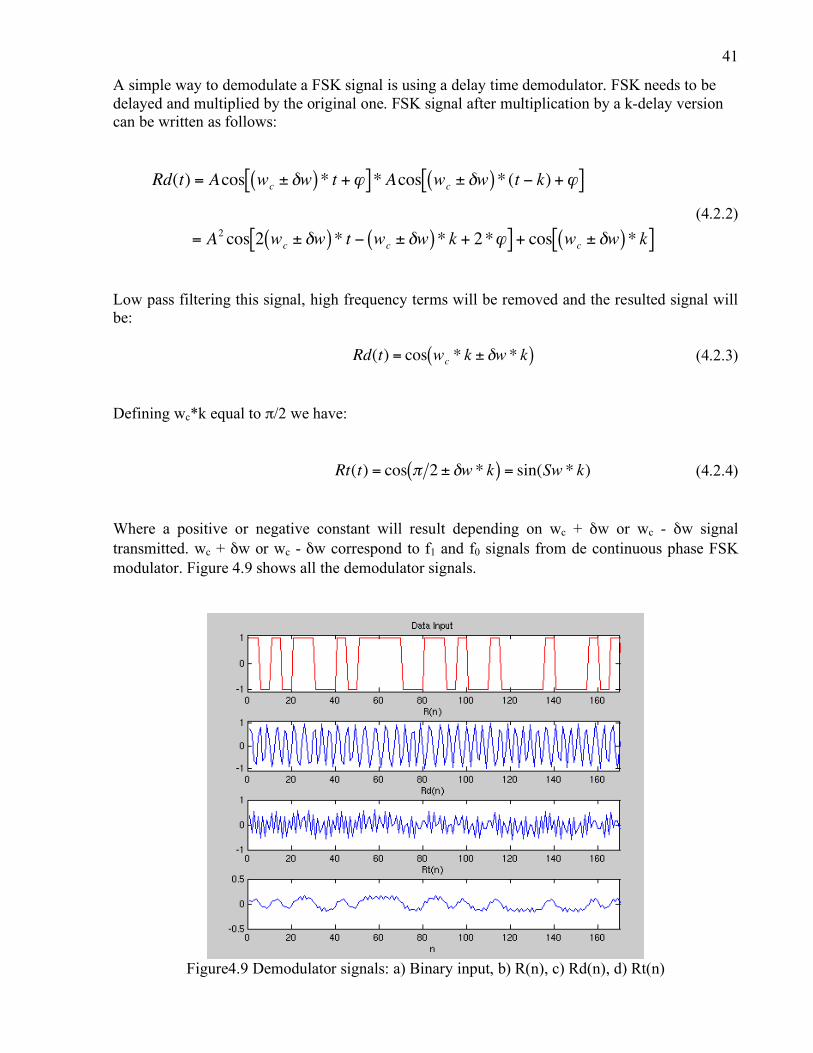
Rt(t) = cos " 2 ± #w * k( ) = sin(Sw * k) (4.2.4) Where a positive or negative constant will result depending on wc + δw or wc - δw signal transmitted. wc + δw or wc - δw correspond to f1 and f0 signals from de continuous phase FSK modulator. Figure 4.9 shows all the demodulator signals.
Figure4.9 Demodulator signals: a) Binary input, b) R(n), c) Rd(n), d) Rt(n)
42
Delay selection depends of various factors as sampling time, bite rate and orthogonally between signals. A trade off is required while less delay time is desirable. A π/2 delay defined in (4.2.4) provides the best orthogonally between the frequencies, this produces the following condition:
!
WC * k = "2
then,
k =1
4 * fc
(4.2.5)
As mentioned before, k corresponds to sampling times and ideally a lower value is desirable. Finally after the demodulation process the original levels need to be recovered; this can be done using a comparator. As can be observed in Figure x c) if the demodulated signal is greater than the threshold a “1” is assigned, else “0” is assigned. Figure 4.10a shows the demodulator output versus the input data with a π/2 delay and Figure 4.10b shows the same input but without a π/2 delay. As can be see, the second plot have a lot of errors because the threshold is not centered in zero. In other hand, the first plot has the same behavior than the input data.
Figure4.10a Demodulator performance with a π/2 delay
43
Figure4.10b Demodulator performance without a π/2 delay
4.2.1 NON-COHERENT DEMODULATION LIMITATIONS In binary FSK signals demodulation the main limitation is that the bitrate must be at least a half of period of the low frequency. It is expressed as follows:
!
f0
=fb
2 (4.2.6)
Then, the bit rate in a channel cannot be more than:
!
f0
= fc "#f2
=fb
2 (4.2.7)
Another limitation is the sample frequency. Lets make the analysis. In the previous section, we found that several delays k can fit the " 2 delay [9]. Figure 4.11, shows a single bit of an input data at certain bit rate (fb).
!
44
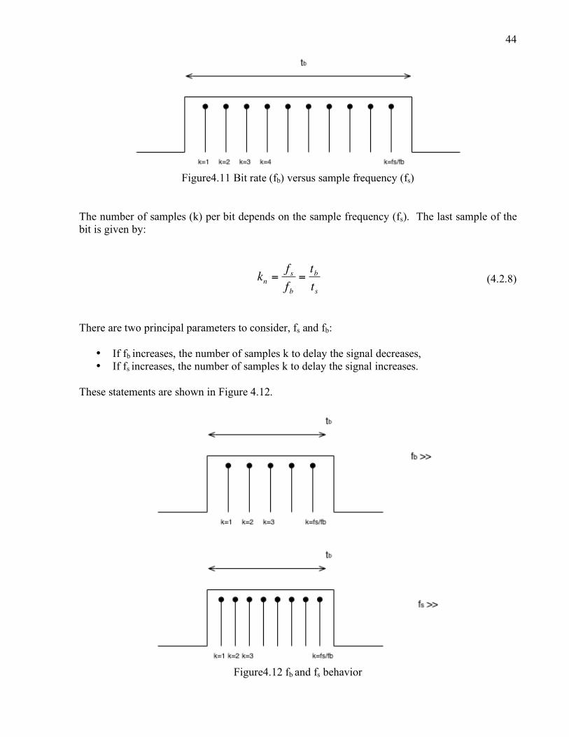
Figure4.11 Bit rate (fb) versus sample frequency (fs)
The number of samples (k) per bit depends on the sample frequency (fs). The last sample of the bit is given by:
!
kn =f s
fb=tb
ts (4.2.8)
There are two principal parameters to consider, fs and fb:
• If fb increases, the number of samples k to delay the signal decreases, • If fs increases, the number of samples k to delay the signal increases.
These statements are shown in Figure 4.12.
Figure4.12 fb and fs behavior
45
As given in this chapter, the non-coherent demodulator needs an integer k delay to have a
!
" 2 delay [10]. With these conditions, the central frequencies available for the integers k’s in a system are:
!
fc =f s
4 • kint
(4.2.9)
Where k={1,2,3… fs/fb}. This relation fulfills the equation (4.2.5) gave for an integer delay k=1. The limitations here are the ones presented in equation (4.1.2) and in (4.2.7). Then, solving the 2 equations system:
!
fbmax =fc
12
+ h2( )
(4.2.10)
The central frequency for integers k-delay to have a
!
" 2 delay is:
!
fc =fs
4 • k (4.2.11)
Replacing (15) in (14) a general formula is found:
!
fbmax =fs
4 • k 12
+ h2( )
(4.2.12)
Therefore, there are three parameters to consider in the reach of a bit rate in this system:
• Sample frequency (fs), • Modulation index (h) and • Sample delay (k).
4.2.2 DECISION ALGORITHM To improve the demodulator performance different algorithms can be used. Decision algorithms may take a variety of forms but the simplest type is known as Integrate-and-dump (IaD). This algorithm sums all samples during one demodulated bit period and decides on the output of the sum whether the incoming bit is an ’0’ o ’1’. If the sum is positive a positive level is assigned to the entire bit. If the sum is negative, a ’0’ level is assigned to the entire bit. The effects of the IaD will be presented in the following chapter.
46
4.3 CONCLUSIONS In this chapter we have presented the GFSK modem theory. Analysis, implementation and simulation have also been presented. Limit and trade offs were also presented. One of the major implementation limitations is the sampling frequency (fs). For the modulator, the main limitation is the length of the sine table related to fs, which limits the generated signals precision. In the demodulator side, the fs is related to the fb. When the fs is increased there will be more samples k available to delay the signal and vice versa. Founding these limitations, the parameters of the modem need to be analyzed and designed. With the parameters, a fully simulation of the modem can be done. This is the object of the following chapter.
4.4 BIBLIOGRAPHY [1] Bluetooth Special Interest Group, “Specification of the Bluetooth System”, Febraury 2002, Core. [2] Kristina Bengtsson, “A DSP based Bluetooth solution, Department of Telecommunications
and Signal Processing”, Master Thesis, Blekinge Institute of Technology. [3] Fuqin Xiong, “Digital Modulation Techniques”, Artech House, USA, 2000. [4] Leon W. Couch II, “Modern Communication Systems. Principles and Applications”, Prentice
Hall, 1995. [5] Phil Evans, Al Lovrich, “Implementation of a FSK modem using the TMS320C17”, Texas
Instrument, Application Report spra080. [6] G. Baudin, F. Virolleau, O. Venard, P. Jardin, “Teaching DSP through the Practical Case
Study of an FSK Modem”, Texas Instrument Application Report, spra347, ESIEE Paris 1996. [7] T. S. Rappaport; “Wireless Communications: Principles and Practice”; Prentice Hall, 2002. [8] Roel Schiphorst, Fokke Hoeksema and Kees Slump, “Bluetooth demodulation algorithms and
their performance”, 2nd Karlsruhe Workshop on Software Radios, pages 99-106, March 2002 University of Twente, Netherlands, 2002.
[9] Charles Tibenderana and Stephan Weiss, “A Low-Complexity High-Performance Bluetooth
Receiver”, in Proceedings of IEE Colloquium on DSP enabled Radio, pages pp. 426-435, Livingston, Scotland, Department of Electronics and Computer Science, University of Southampton, UK, 2003.
[10] Daniel Santana, Javier Gonzalez, “Digital Modulation DSP analysis and implementation
based on integer k-sampling”, in ICED 2004, Internacional Conference on Electronic Design, Veracrúz, Veracrúz, Nov. 21 – 22..
47
5. SIMULATION In this chapter two digital modem simulations are presented. First, a GFSK modem working at 9.6KHz is presented. This simulation has been implemented in the DSP. Second, a Bluetooth modem simulation is presented. The Bluetooth case has not been implemented due to DSK limitations, however if the DSK codec sample frequency is increased the implementation for the Bluetooth is realizable. This codec is called “daughter card” and is connected to the DSK through a special connectors. All the simulations were performed on Matlab and then translated to DSP code. In another hand, once the module or stages is programmed in language C, the code can easily be translated to the DSP programming language. Some specific functions required by the modem, like fft, ber, filter, and psd were developed. After this introduction, the simulations details are presented, then the results after simulation and implementation. All programs used in this chapter are totally presented in Appendix A.
5.1 MATLAB SIMULATION OF A GFSK MODEM AT 9.6 KHZ In this section, the 9.6KHz GFSK Modem simulation on Matlab is presented. The first module to be considered is the FSK modulator; in this case an index modulation needs to be selected. The index h=0.4375 has been considered due to have the next parameters:
"f = 4200Hz
fb = 9600Hz
!
48
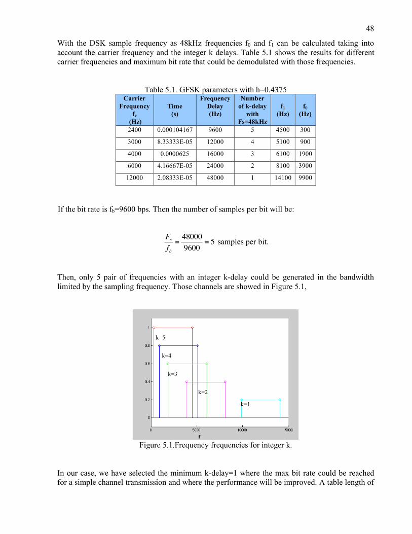
With the DSK sample frequency as 48kHz frequencies f0 and f1 can be calculated taking into account the carrier frequency and the integer k delays. Table 5.1 shows the results for different carrier frequencies and maximum bit rate that could be demodulated with those frequencies.
Table 5.1. GFSK parameters with h=0.4375 Carrier
Frequency fc
(Hz)
Time
(s)
Frequency Delay (Hz)
Number of k-delay
with Fs=48kHz
f1 (Hz)
f0 (Hz)
2400 0.000104167 9600 5 4500 300
3000 8.33333E-05 12000 4 5100 900
4000 0.0000625 16000 3 6100 1900
6000 4.16667E-05 24000 2 8100 3900
12000 2.08333E-05 48000 1 14100 9900
If the bit rate is fb=9600 bps. Then the number of samples per bit will be:
!
Fs
fb=48000
9600= 5 samples per bit.
Then, only 5 pair of frequencies with an integer k-delay could be generated in the bandwidth limited by the sampling frequency. Those channels are showed in Figure 5.1,
Figure 5.1.Frequency frequencies for integer k.
In our case, we have selected the minimum k-delay=1 where the max bit rate could be reached for a simple channel transmission and where the performance will be improved. A table length of
k=5
k=4
k=3
k=2
k=1
f
49
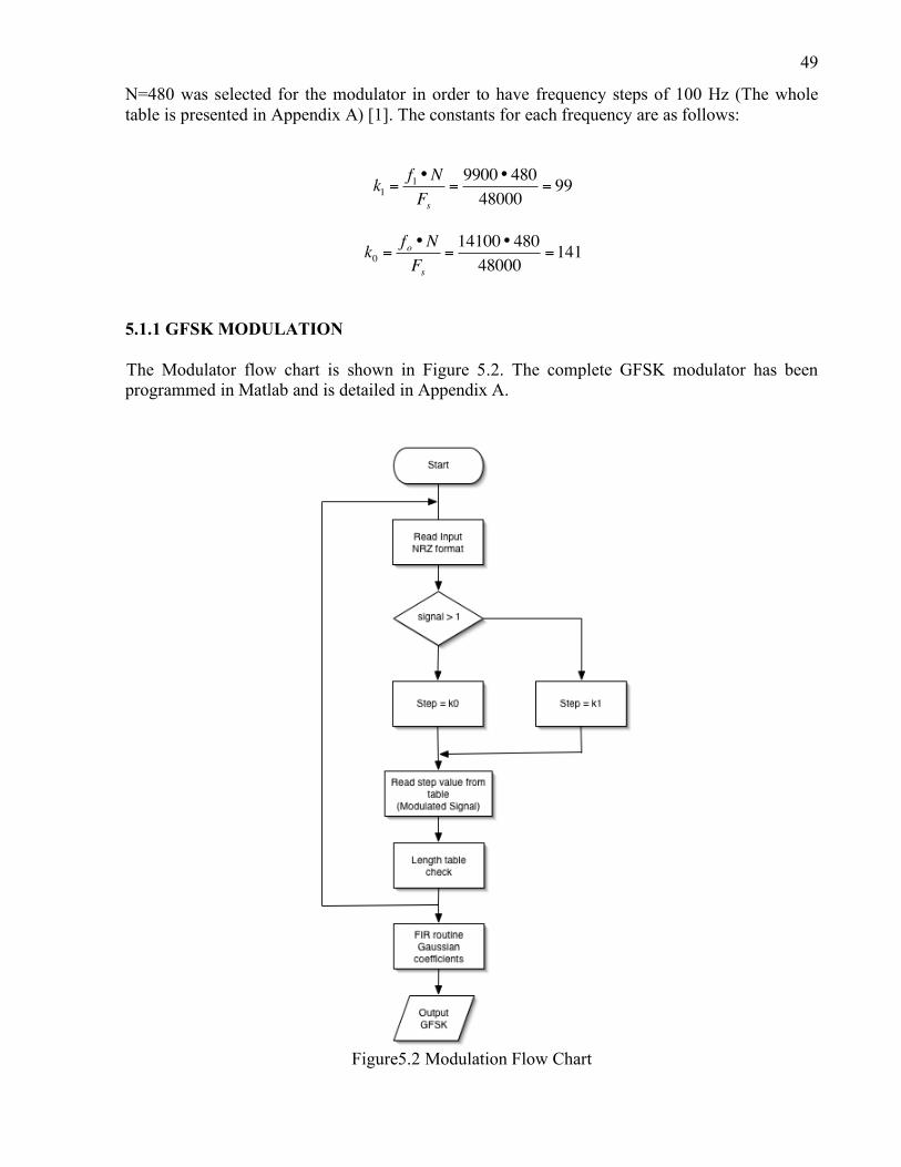
N=480 was selected for the modulator in order to have frequency steps of 100 Hz (The whole table is presented in Appendix A) [1]. The constants for each frequency are as follows:
!
k1
=f1•N
Fs=9900• 480
48000= 99
!
k0
=fo •N
Fs=14100• 480
48000=141
5.1.1 GFSK MODULATION The Modulator flow chart is shown in Figure 5.2. The complete GFSK modulator has been programmed in Matlab and is detailed in Appendix A.
Figure5.2 Modulation Flow Chart
50
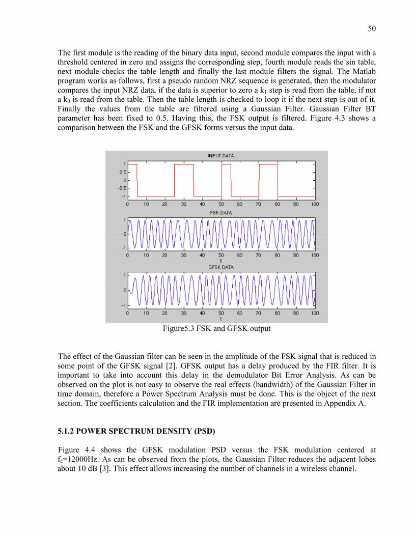
The first module is the reading of the binary data input, second module compares the input with a threshold centered in zero and assigns the corresponding step, fourth module reads the sin table, next module checks the table length and finally the last module filters the signal. The Matlab program works as follows, first a pseudo random NRZ sequence is generated, then the modulator compares the input NRZ data, if the data is superior to zero a k1 step is read from the table, if not a k0 is read from the table. Then the table length is checked to loop it if the next step is out of it. Finally the values from the table are filtered using a Gaussian Filter. Gaussian Filter BT parameter has been fixed to 0.5. Having this, the FSK output is filtered. Figure 4.3 shows a comparison between the FSK and the GFSK forms versus the input data.
Figure5.3 FSK and GFSK output
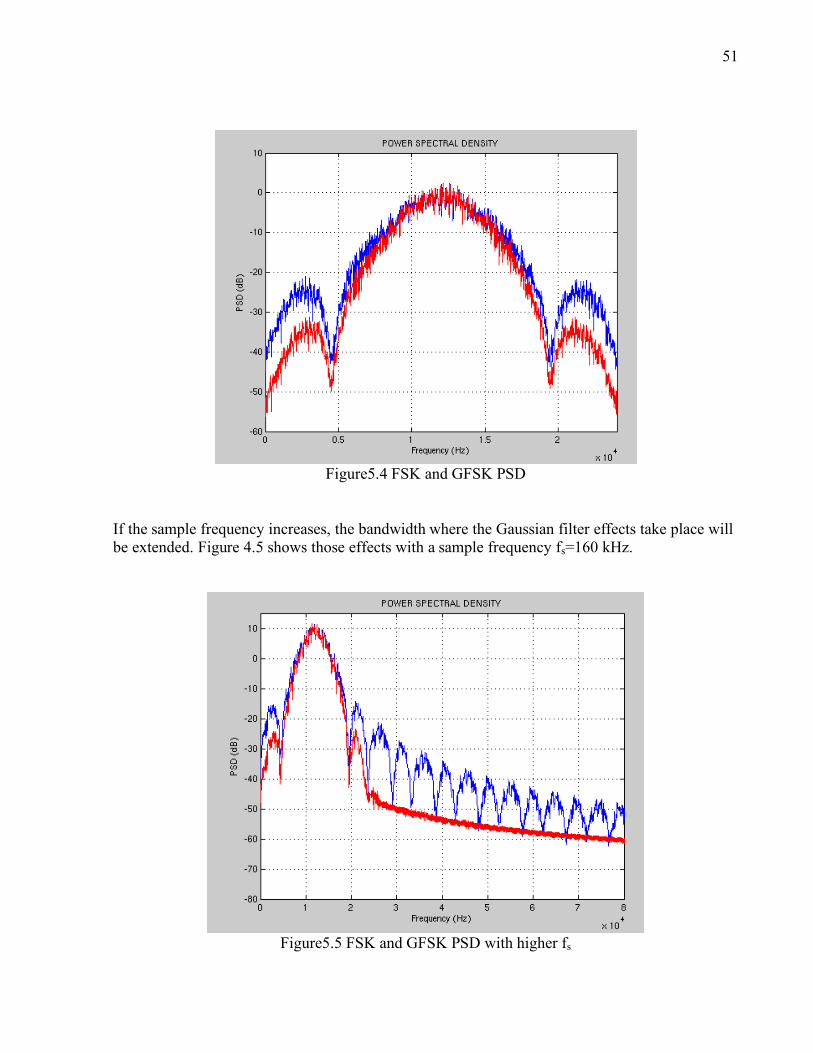
The effect of the Gaussian filter can be seen in the amplitude of the FSK signal that is reduced in some point of the GFSK signal [2]. GFSK output has a delay produced by the FIR filter. It is important to take into account this delay in the demodulator Bit Error Analysis. As can be observed on the plot is not easy to observe the real effects (bandwidth) of the Gaussian Filter in time domain, therefore a Power Spectrum Analysis must be done. This is the object of the next section. The coefficients calculation and the FIR implementation are presented in Appendix A. 5.1.2 POWER SPECTRUM DENSITY (PSD) Figure 4.4 shows the GFSK modulation PSD versus the FSK modulation centered at fc=12000Hz. As can be observed from the plots, the Gaussian Filter reduces the adjacent lobes about 10 dB [3]. This effect allows increasing the number of channels in a wireless channel.
51
Figure5.4 FSK and GFSK PSD
If the sample frequency increases, the bandwidth where the Gaussian filter effects take place will be extended. Figure 4.5 shows those effects with a sample frequency fs=160 kHz.
Figure5.5 FSK and GFSK PSD with higher fs
52
5.1.3 DEMODULATION The demodulation flow chart is shown in Figure 5.6. As it was presented in chapter 5, the demodulator is composed of a FM Discriminator (non-coherent demodulator), where the first module reads the modulated signal, module 2 is a phase shifter, third module is a multiplier, fourth module is a FIR routine, and finally the comparator and the Decision algorith modules. Main program could be reviewed in Appendix 1.
Figure5.6 Demodulator flow chart
The demodulator functionality is as follows, the ADC samples the input FSK signals, then and the samples are divided in two paths, one original and one delayed [4]. Then booth versions are multiplied (In this case k=1). After the multiplier, the samples are low pass filtered and passed through the decision algorithm (IaD). The low pass filter has a cut off frequency equals to the bit
53
rate. The decision algorithm implementation and the low pass filter design are shown in Appendix 1. To evaluate the impact of the decision algorithm, a comparator after the low pass filter was implemented too. Figure 5.7 shows the demodulator signals. In the first plot the data input is plotted versus the GFSK demodulated signal. In the next plot, the GFSK demodulated signal after the comparator is shown. Finally, the GFSK demodulated signal after the decision algorithm is shown.
Figure5.7 a) GFSK demodulated signal and data input, b) GFSK demodulated signal after the
comparator, c) GFSK demodulated signal after IaD
For a GFSK demodulator, the received signal needs to be synchronized due to the delay produced by the Gaussian filter. Up to this point, the simulation has been considered noiseless. That’s because there are notable differences between the signal after the comparator and after the IaD. To obtain the error performance of the GFSK demodulator, the modulated signal was passed through an AWGN channel. This simulation is presented in the next section.
54
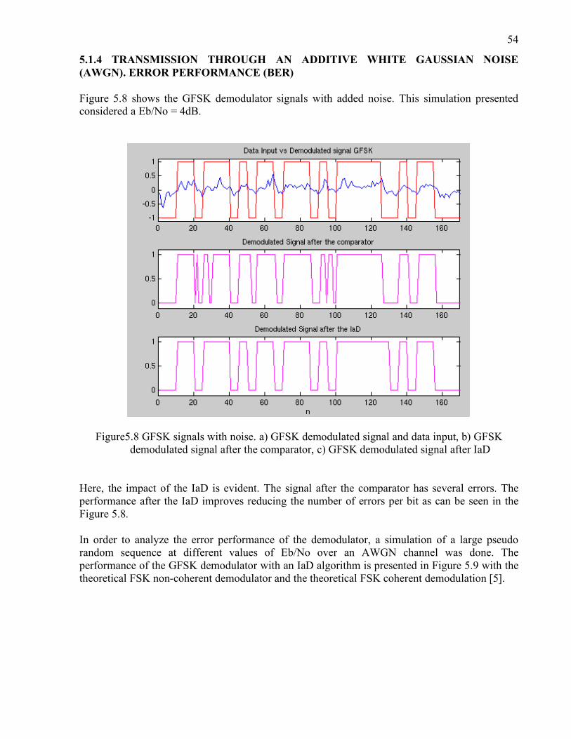
5.1.4 TRANSMISSION THROUGH AN ADDITIVE WHITE GAUSSIAN NOISE (AWGN). ERROR PERFORMANCE (BER) Figure 5.8 shows the GFSK demodulator signals with added noise. This simulation presented considered a Eb/No = 4dB.
Figure5.8 GFSK signals with noise. a) GFSK demodulated signal and data input, b) GFSK demodulated signal after the comparator, c) GFSK demodulated signal after IaD
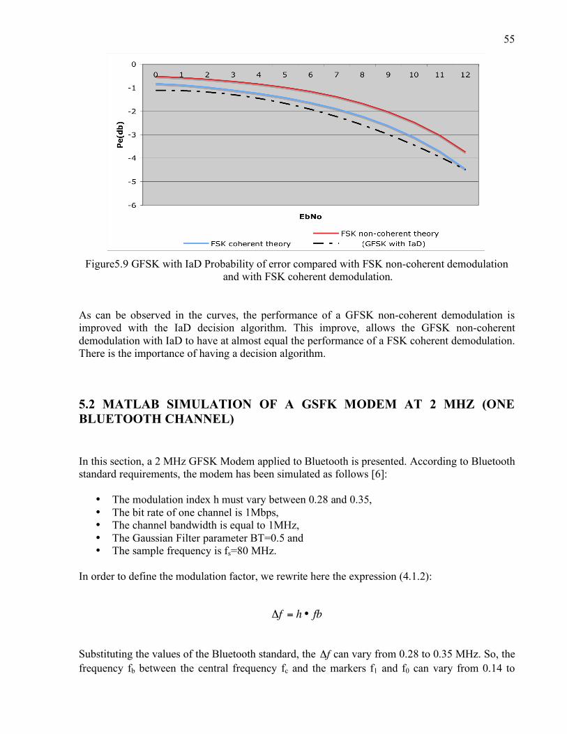
Here, the impact of the IaD is evident. The signal after the comparator has several errors. The performance after the IaD improves reducing the number of errors per bit as can be seen in the Figure 5.8. In order to analyze the error performance of the demodulator, a simulation of a large pseudo random sequence at different values of Eb/No over an AWGN channel was done. The performance of the GFSK demodulator with an IaD algorithm is presented in Figure 5.9 with the theoretical FSK non-coherent demodulator and the theoretical FSK coherent demodulation [5].
55
Figure5.9 GFSK with IaD Probability of error compared with FSK non-coherent demodulation and with FSK coherent demodulation.
As can be observed in the curves, the performance of a GFSK non-coherent demodulation is improved with the IaD decision algorithm. This improve, allows the GFSK non-coherent demodulation with IaD to have at almost equal the performance of a FSK coherent demodulation. There is the importance of having a decision algorithm.
5.2 MATLAB SIMULATION OF A GSFK MODEM AT 2 MHZ (ONE BLUETOOTH CHANNEL) In this section, a 2 MHz GFSK Modem applied to Bluetooth is presented. According to Bluetooth standard requirements, the modem has been simulated as follows [6]:
• The modulation index h must vary between 0.28 and 0.35, • The bit rate of one channel is 1Mbps, • The channel bandwidth is equal to 1MHz, • The Gaussian Filter parameter BT=0.5 and • The sample frequency is fs=80 MHz.
In order to define the modulation factor, we rewrite here the expression (4.1.2):
!
"f = h • fb Substituting the values of the Bluetooth standard, the "f can vary from 0.28 to 0.35 MHz. So, the frequency fb between the central frequency fc and the markers f1 and f0 can vary from 0.14 to
!
56
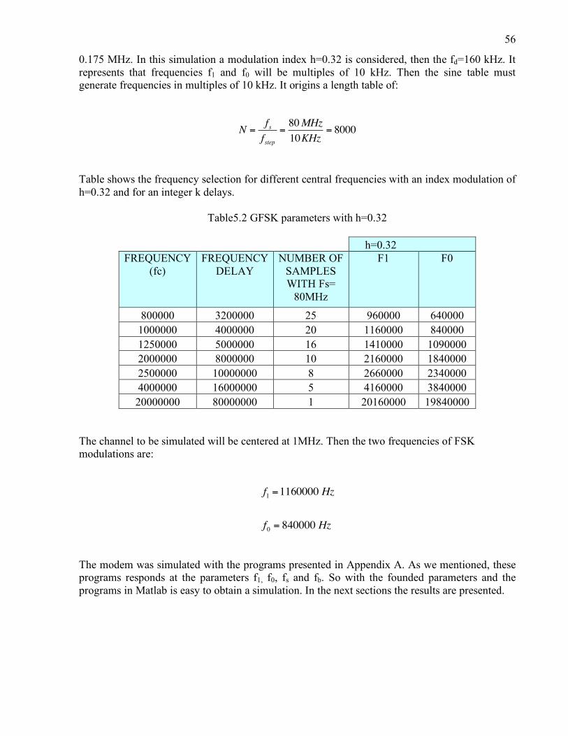
0.175 MHz. In this simulation a modulation index h=0.32 is considered, then the fd=160 kHz. It represents that frequencies f1 and f0 will be multiples of 10 kHz. Then the sine table must generate frequencies in multiples of 10 kHz. It origins a length table of:
!
N =fs
fstep=80MHz
10KHz= 8000
Table shows the frequency selection for different central frequencies with an index modulation of h=0.32 and for an integer k delays.
The channel to be simulated will be centered at 1MHz. Then the two frequencies of FSK modulations are:
!
f1
=1160000 Hz
f0
= 840000 Hz
The modem was simulated with the programs presented in Appendix A. As we mentioned, these programs responds at the parameters f1, f0, fs and fb. So with the founded parameters and the programs in Matlab is easy to obtain a simulation. In the next sections the results are presented.
57
5.2.1 MODULATION The first module to be considered is the modulator. The two frequencies of FSK modulations are then:
!
f1
=1160000 Hz
f0
= 840000 Hz
Then, in order to define the steps for the sine table, the following table can be used:
!
k1
=f •N
fs=1160000•80000
80000000=116
!
k =f •N
fs=840000•80000
80000000= 84
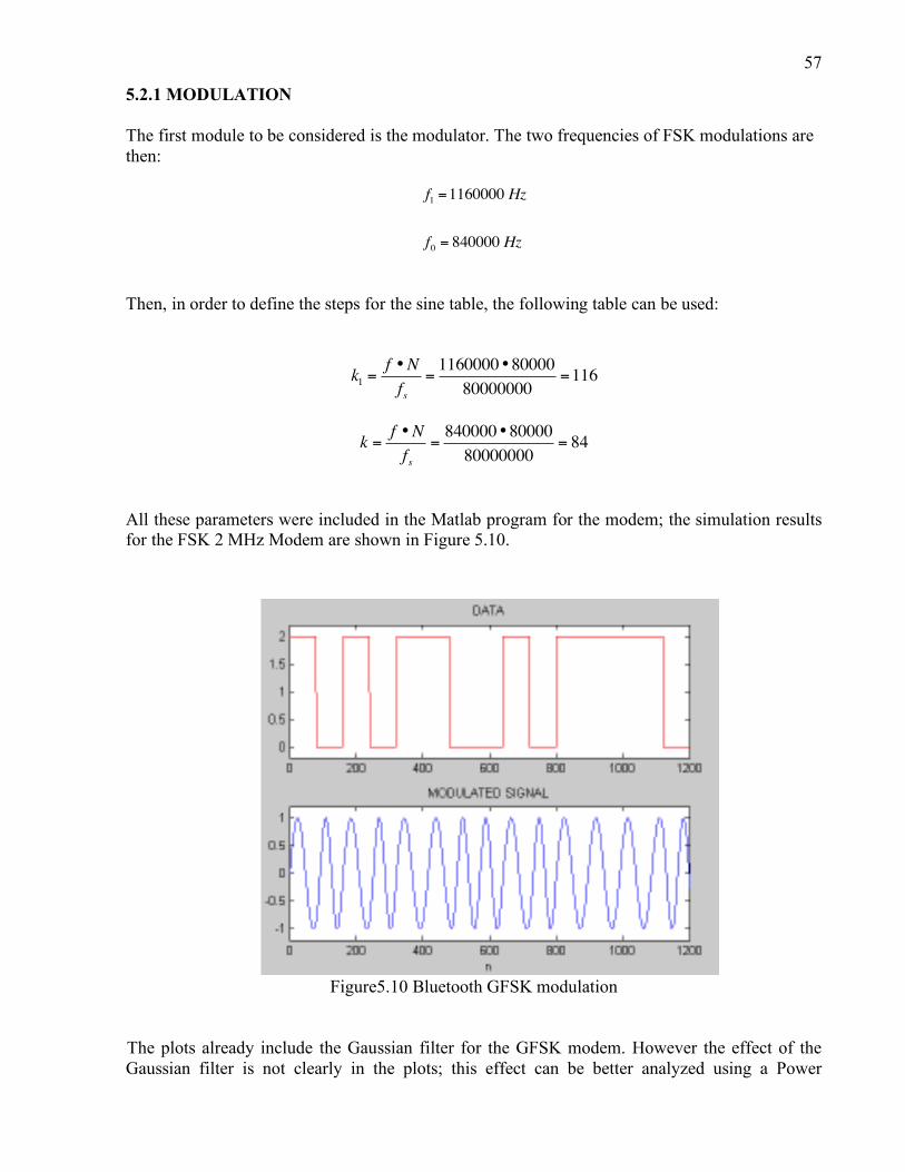
All these parameters were included in the Matlab program for the modem; the simulation results for the FSK 2 MHz Modem are shown in Figure 5.10.
Figure5.10 Bluetooth GFSK modulation The plots already include the Gaussian filter for the GFSK modem. However the effect of the Gaussian filter is not clearly in the plots; this effect can be better analyzed using a Power
58
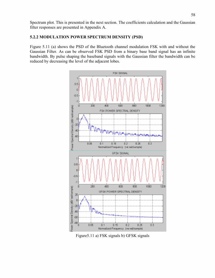
Spectrum plot. This is presented in the next section. The coefficients calculation and the Gaussian filter responses are presented in Appendix A. 5.2.2 MODULATION POWER SPECTRUM DENSITY (PSD) Figure 5.11 (a) shows the PSD of the Bluetooth channel modulation FSK with and without the Gaussian Filter. As can be observed FSK PSD from a binary base band signal has an infinite bandwidth. By pulse shaping the baseband signals with the Gaussian filter the bandwidth can be reduced by decreasing the level of the adjacent lobes.
Figure5.11 a) FSK signals b) GFSK signals
59
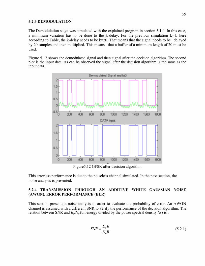
5.2.3 DEMODULATION The Demodulation stage was simulated with the explained program in section 5.1.4. In this case, a minimum variation has to be done to the k-delay. For the previous simulation k=1, here according to Table, the k-delay needs to be k=20. That means that the signal needs to be delayed by 20 samples and then multiplied. This means that a buffer of a minimum length of 20 must be used. Figure 5.12 shows the demodulated signal and then signal after the decision algorithm. The second plot is the input data. As can be observed the signal after the decision algorithm is the same as the input data.
Figure5.12 GFSK after decision algorithm
This errorless performance is due to the noiseless channel simulated. In the next section, the noise analysis is presented. 5.2.4 TRANSMISSION THROUGH AN ADDITIVE WHITE GAUSSIAN NOISE (AWGN). ERROR PERFORMANCE (BER) This section presents a noise analysis in order to evaluate the probability of error. An AWGN channel is assumed with a different SNR to verify the performance of the decision algorithm. The relation between SNR and Eb/N0 (bit energy divided by the power spectral density N0) is :
SNR =EbR
N0B
(5.2.1)
!
60 Where SNR is Signal-to-Noise Ratio, Eb the bit energy, No the power spectral density, R the bit rate and B the Bandwidth. In the case of Bluetooth [7]:
!
B =1
R (5.2.2)
Then,
!
SNR =EbR
N0B
=Eb
N0
(5.2.3)
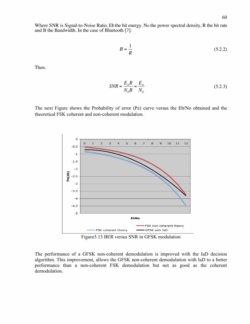
The next Figure shows the Probability of error (Pe) curve versus the Eb/No obtained and the theoretical FSK coherent and non-coherent modulation.
Figure5.13 BER versus SNR in GFSK modulation
The performance of a GFSK non-coherent demodulation is improved with the IaD decision algorithm. This improvement, allows the GFSK non-coherent demodulation with IaD to a better performance than a non-coherent FSK demodulation but not as good as the coherent demodulation.
61
5.3 CONCLUSIONS This chapter has presented two simulations. First, a 9600 bps GFSK Modem at. This modem was also implemented in the DSP TI 5000XX. The Matlab programs for the simulation were created to have an easy translation to the DSP language. Second, a 2 MHz GFSK Bluetooth Modem according to the standard. Both simulations were analyzed considering an AWGN noise channel. The results for the FSK coherent and non-coherent theoretical probabilities of error were also presented. The results were acceptable for the used parameters. It is important to mention that this performance could considerably be affected if the integer k-delay analysis is not adequately done. That is, if a time delay is experimented causing an offset in the threshold of the IaD this could affect directly the Probability of error. In another hand, the Inter-symbol Interference (ISI) caused by the closest channels in the bandwidth has not been considered. Finally, the analysis presented in this chapter has allowed us to verify that all the stages in the modulator and demodulator have an excellent performance. Next works will focus in the placement of this design over other conditions to find its weaknesses. Now that the simulation has been compared to the theory and all the stages have been tested, the next step is the implementation in the DSP. This is the object of the next chapter .
5.4 BIBLIOGRAPHY
[1] Phil Evans, Al Lovrich, “Implementation of a FSK modem using the TMS320C17”, Texas
Instrument, Application Report spra080. [2] T. S. Rappaport; “Wireless Communications”; Prentice Hall, 2002. [3] Roel Schiphorst, Fokke Hoeksema and Kees Slump, “Bluetooth demodulation algorithms and
their performance”, in 2nd Karlsruhe Workshop on Software Radios, pages 99-106, March 2002 University of Twente, Netherlands, 2002.
[4] G. Baudin, F. Virolleau, O. Venard, P. Jardin, “Teaching DSP through the Practical Case
Study of an FSK Modem”, Texas Instrument Application Report, spra347, ESIEE Paris 1996. [5] Dr. Mike Fitton, “Telecommunications Research Lab”, Report, Toshiba Research Europe
Limited, [6] Bluetooth Special Interest Group, “Specification of the Bluetooth System”, February 2002,
Core. [7] Charles Tibenderana and Stephan Weiss, “A Low-Complexity High-Performance Bluetooth
Receiver”, in Proceedings of IEE Colloquium on DSP enabled Radio, pages pp. 426-435, Livingston, Scotland, Department of Electronics and Computer Science, University of Southampton, UK, 2003.
62
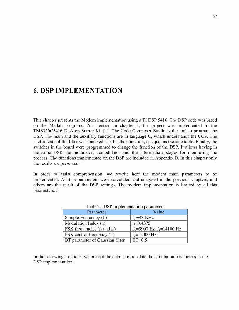
6. DSP IMPLEMENTATION This chapter presents the Modem implementation using a TI DSP 5416. The DSP code was based on the Matlab programs. As mention in chapter 3, the project was implemented in the TMS320C5416 Desktop Starter Kit [1]. The Code Composer Studio is the tool to program the DSP. The main and the auxiliary functions are in language C, which understands the CCS. The coefficients of the filter was annexed as a heather function, as equal as the sine table. Finally, the switches in the board were programmed to change the function of the DSP. It allows having in the same DSK the modulator, demodulator and the intermediate stages for monitoring the process. The functions implemented on the DSP are included in Appendix B. In this chapter only the results are presented. In order to assist comprehension, we rewrite here the modem main parameters to be implemented. All this parameters were calculated and analyzed in the previous chapters, and others are the result of the DSP settings. The modem implementation is limited by all this parameters. :
Table6.1 DSP implementation parameters Parameter Value
Sample Frequency (fs) fs =48 KHz Modulation Index (h) h=0.4375 FSK frequencies (f0 and f1) f0 =9900 Hz, f1=14100 Hz FSK central frequency (fc) fc=12000 Hz BT parameter of Gaussian filter BT=0.5
In the followings sections, we present the details to translate the simulation parameters to the DSP implementation.
!
63
6.1 IMPLEMENTATION DETAILS In Code Composer Studio, the management of the project is as equal as a C project. It means that we have a main program that calls other C functions, and that allows to use libraries and header files. As we mention in Chapter 5 DSP/BIOS is a configuration tool to generate code for the DSP. In this work we made a DSP/BIOS based implementation. The configuration of the channel plugged to the codec, the interrupts management and the scheduling was totally made in DSP/BIOS configuration tool. In the DSK the codec is plugged to one channel of the Multi-channel buffered serial port (McBSP) from where the samples are taken directly. It means that the samples are not passed though a memory (DMA), then the implementation don’t have a frame improvement, producing a process time of one sample. Besides, the project uses the Chip Support Library (CSL) that contains customary functions to the codec and the Board Support Library (BSL) that have customary functions to the switches. The function for the FIR filter was obtained in the Matlab Central file exchange, it is owned by Richard Sikora. It is an optimized FIR routine in assembler language, and works to a maximum 51 coefficients, with the option to reduce the use of the coefficients that represents less function time. The coefficients was obtained in Matlab and included in the project as a heather file. The rest function as the modulator, the delay and the multiplication was all programmed in C language and prototyped in main program.
6.2 MODULATOR As was mentioned in chapter 5, the modulator is based on a sine table. Once the values are calculated and simulated, they need to be translated to the DSP language. As mention in chapter 3, the PCM3002 (DSK codec) is a 16-bit codec, 15 bits are used for the values and the 16th bit is used for the sign [2]. Then, the values must be converter to a 15-bit format. It is done by multiplying the decimal values to 215 and rounded it. Next instruction in Matlab was used to do it:
round(215
• sin table) , where sintable is the vector with the 480 sine values and changes for the coefficients of the Gaussian Filter depending on the variable where the coefficients are stored. Appendix B shows the sintable and FIR coefficients in 15-bit format annexed to the project as a header file. Once that the values have the correct format, there have to be stored in the internal memory of the DSP. After this, we control the table using it as a look-up table. The flow chart of the modulator is the same as the simulated in chapter 5.1.1. The mainly difference is that in Matlab the values are managed in vectors that can be seen as a big buffers. The implementation differs in this case because the values are managed as samples and processed sample by sample. It is that the signal processing is done in less than a sample. Figure 6.1 shows the flow chart of the main program indicating the functions that makes the process.
64
Figure6.1 DSP modulator flow chart The DSK has 4 audio jacks to take out the information. Those are: microphone, line-in, line-out and speaker jacks [1]. In this implementation line-in and line-out was used. In the line-in jack the input data in a NRZ format was introduced to the DSP. Then this data was processed and was taken out to the line-out jack. So, the line-in was connected to a binary pseudo random generator and to an oscilloscope and the line out to other channel of the oscilloscope. In other hand, to have the frequency performance a spectrum analyzer was used. The line-in was connected to a coaxial interface and then to the analyzer. Figure 6.2 shows the data input and the GFSK modulation.
mod_data()
FIR_filters_asm
65
Figure6.2 GFSK modulation
In the plot, the channel 1 shows the binary data input in NRZ format, channel 2 shows the GFSK modulation from the DSP. It can be observed the changes in magnitude caused by the Gaussian filter. The modulated signal is delayed because of the codec. The codec is connected trough the serial port of the DSP that is slower than the processor; it generates a delay in the output signal. This delay could be observed more clearly in the demodulation stage. We need to see the frequency performance of the modulation to have a better idea of the FSK modulation and the Gaussian filter effects. Figure 6.3 shows the spectrum of the GFSK signal.
Figure6.3 FSK spectrum
66
The marker shows the central frequency
!
fc =12.5 that corresponds to established central frequency or carrier. The Gaussian filter effect reduces the side lobes of the signal. A mirror image caused for the digital FIR filter appears at the double of fc as can be seen in Figure 6.4.
Figure6.4 Mirror effect in GFSK modulation
The mirror signal is centered at 25KHz and is attenuated about -45 dB from the main spectrum. To visualize the effect of the Gaussian filter, a FSK modulation was taken out from the DSP. Figure 6.5, shows the FSK modulation with the GFSK modulation. The smoothest line is the FSK spectrum.
Figure6.5 FSK and GFSK spectrum
67
The main nodule doesn’t have a significant impact from de Gaussian filter, but the second is reduced in approximately -10 dB [3]. The following nodules are reduced, but the mirror images are still appearing. It is because of the sample frequency fs. If it increases the effects of the Gaussian filter will be extended as was shown in chapter 5.
6.3 DEMODULATOR A non-coherent modulator (FM discriminator) was implemented [4]. Because the DSK uses a 15-bits ADC, the length of the variables must be controlled. The demodulator involves a multiplication and a FIR filter (multiplications and sums), if we multiply two numbers of 15 bits the result will be in 30 bits, then if it will be multiplied to other 15-bit variable and summed, the total length of the final variable will be approximately of 64 bits. Then, the variables must be truncated in every operation to have the less lost of information as possible. Considering this, the demodulator flow chart is almost the same as the Matlab simulation remembering that the variables are used sample per sample. Appendix B presents all the C functions and the FIR coefficients (LPF) used in this stage. Figure 6.6 shows the flow chart of the DSP demodulator implementation indicating the functions that makes the process.
Figure6.6 DSP demodulator Flow chart
delay_input
FIR_dual_filter_variable_asm
main (switch=1)
68
To complete the implementation setup, two DSK were needed, one for the modulator and one for the demodulator. The control switches allow changing the function that we want in the output. Each DSP was programmed with all the functions. One DSP was programmed as a stand-alone system that means that it works without a computer. The other was still working with the computer to have some graphics and statistics. The line-out of the modulator DSK was connected to the line-in of the demodulator DSK. The line-in of the modulator DSK was connected to the pseudo random binary data generator and to the channel 1 of the oscilloscope. Finally, the line-out of the demodulator was connected to the channel 2 of the oscilloscope. Figure 6.7 shows these connections.
Figure6.7 Modem GFSK setup
Once that the setup was working, the demodulator signal was taken from the spectrum analyzer. Figure 6.8 shows the demodulator signals.
Figure6.8 GFSK Demodulator output
69
From the plots in Figure 6.8, we can observe the output of the demodulator after the LPF. It has the behavior of the input signal showed below but with a delay caused by the codec. As can be appreciate, it has a small magnitude (around the 340 mV) compared with the one in Figure 6.9 that considers an IaD. This is due to the IaD algorithm; a value is assigned after the sum of 5 demodulator values.
Figure6.9 GFSK demodulator with IaD
Even so, the signal haven’t has a square form because of the codec. Since it use a delta-sigma modulation, the output of a square signals is a ramp, it cannot create a constant. This stage was implemented only to see the performance of the demodulator, if in the system we need to connect a digital destination; the DAC doesn’t need to be present. It can be connected directly though the serial or parallel ports, improving the performance and the speed of demodulation.
6.4 CONCLUSIONS A 9.6 KHz GFSK Modem was successfully implemented in the TMS320C5416 DSK. The complete modem was implemented in two DSK for testing purposes; one was selected as the modulator and other as the demodulator. A setup was built with an oscilloscope and spectrum analyzer to analyze the modem performance. The demodulator was tested with different sequences provided by a digital data transmission auxiliary module DL2560B to verify the complete performance. All the tests were successful, however next chapter presents a comparison between the results obtained in the Matlab simulation and the DSP implementation.
70
6.5 BIBLIOGRAPHY [1] “TMS320VC5416 DSK”, Spectrum Digital Technical Reference, 2002. [2] “16-/20-Bit Single-Ended Analog Input/Output SoundPlus™ Stereo Audio CODECs”, Texas
Instrument Technical Documents, 2000. [3] T. S. Rappaport; “Wireless Communications: Principles and Practice”; Prentice Hall, 2002. [4] Roel Schiphorst, Fokke Hoeksema and Kees Slump, “Bluetooth demodulation algorithms and
their performance” in 2nd Karlsruhe Workshop on Software Radios, pages 99-106, March 2002 University of Twente, Netherlands, 2002.
[5] Phil Evans, Al Lovrich, “Implementation of a FSK modem using the TMS320C17”, Texas
Instrument, Application Report spra080. [6] G. Baudin, F. Virolleau, O. Venard, P. Jardin, “Teaching DSP through the Practical Case
Study of an FSK Modem”, Texas Instrument Application Report, spra347, ESIEE Paris 1996. [7] Kristina Bengtsson, “A DSP based Bluetooth solution, Department of Telecommunications
and Signal Processing”, Master Thesis, Blekinge Institute of Technology.
71
7. CONCLUSIONS AND RESULTS
This chapter presents in the first section the comparison between Matlab simulation results and DSP implementation. Next in section two, a DSP implementation timing analysis is presented, and then the prototyping functions and processing time by module and for the complete modem are presented. Finally an analysis based on the ADC-DAC available in the market was done to define the fastest applications.
7.1 MATLAB SIMULATION VERSUS DSP IMPLEMENTATION In this section, the modulator comparison was done based on the PSD of the simulation in Matlab and the implementation in the DSP. Then, the comparison of the demodulator was done based on the demodulator signals. Figure 7.1, shows the PSD of the GFSK and FSK modulations obtained in the DSP analysis and in the Matlab simulation. The smoothest line is the FSK spectrum.
(a)
72
(b)
Figure 7.1 GFSK modulation PSD a) DSP, b) Matlab
As can be observed in the plots, the power spectrums are quite similar. For both plots, the main lobe is conserved however the effect of the Gaussian filter is observed in the second lobe; it is attenuated by about 10dB. This comparison verifies the implementation performance based in the simulation and the theory. Figure 7.2, shows the signal after the LPF in the demodulator.
(a)
(b)
Figure7.2 GFSK demodulator signals. a) DSP, b) Matlab Now for the demodulator, the signals are compared at the output and input signals. In both cases, the demodulated signal follows the behavior of the input signal; it is a low magnitude signal compared with the input in Matlab; in the DSP implementation this statement is true but
73
compared with the maximum output that could be reached by the DAC that is 3 volts [1]. It is not compared with the input signal because the modulator only response to the threshold, not to the level. Finally both need a processing to have the final result. This is done by decision algorithm (IaD). With the two comparisons presented, the performance of the DSP implementation is verified. The next step is to check the timing process of the different functions to know the limits and the future optimizations that need to work to fasters bit rates.
7.2 DSP TIMING ANALYSIS In this section a function profile is presented. The objective is to build a complete module parameterization of the DSP implementation. The DSK instruction cycle time is of 140 MHz (6.25 ns) [2]. Every implemented function was profiled to know how many cycles takes. Table 7.1, shows the results:
Table 7.1. Implementation function profile Function Instruction Number of Frequency %
cycle time cycles CPU read 6.25 ns 3400 47.1 kHz 100 write 6.25 ns 3400 47.1 kHz 100
The FIR routine is the slowest one. This routine was not implemented in this thesis, it was taken from the Matlab source [3], and so it is not optimized for our project. The other functions were totally implemented for the project in C language. Then, an assembler implementation can be done. The instruction cycle time is dependent on the DSP used, then newest DSPs as the TMS6000 family are faster which gives a fewer cycles times. In this implementation, while the FIR routine is the slowest function it is the limit of speed. It is that with this DSK and with these functions (without optimization) the faster codec that could be attached is a 1MHz codec. It is for this kind of implementation where the time available for processing is the time between samples (fs). An alternative implementation is based on buffers where the processing time depends on the number of buffers (n) used and in its lengths (N). Here the processing time goes up to (n/2)Nfs []. Then a buffer based implementation could be a great improvement to the design presented in this work. In the next section a high-speed analysis is presented considering the modulation and demodulation facts.
74
7.3 HIGH SPEED IMPLEMENTATION ANALYSIS In this section, we discuss the k-sampling technique related to the sample frequency used to optimize the bit rate of the modem. Remembering the founded formula for the maximum bit rate of the implementation (4.2.12):
!
fbmax =fs
4 • k 12
+ h2( )
From the formula, if the sample frequency increases, the bit rate increases; if the h increases the bit rate decreases and if the k-delay increases the bit rate will decrease [4]. For example, in the system simulated and implemented, the maximum bit rates depending on these three conditions are shown in Table:
Finally, an analysis for faster data converters compatibles with the TMS320C5000 and TMS320C6000 is presented. For the case Bluetooth, the following table shows the founded data converters, its sample frequency, the maximum bit rate that could be reached and the suitable applications.
Table7.3 High-speed codec’s, application and maximum bit rate
7.4 THESIS IMPACT AT ITESM This work represents the establishment of research works in the field of Software Radio applied to wireless communications for the 4a generation implemented at the ITESM-CEM. This work was developed based on advanced investigations for the fully implementation of a digital communication system (encoder, decoder, correction error codes, interleaving, etc…). The main focus of this work has been addressed to the domain of the Modulation schemes and in the learning of the DSP as an implementation tool. With the know-how in the DSP implementation, we are allowed to teach the fundamentals, spreading the knowledge in the University. We hope that this work will allow the MCE, ICE and ISE students to discover new forms of design that will contribute in the accomplishment of stages in our final prototype,
7.5 IMPLEMENTATION CONCLUSIONS The implementation presented in this work is totally parameterized, that means, that all the work has been verified theoretical and by simulation. This has allowed us to have the control of the simulation and implementation, and optimize the results for different applications. The only performance that was not parameterized in the implementation was the Bit Error Rate (BER). This is due the limitations of the measure equipment available at the laboratory; the instrument used doesn’t allow the performance at low bit rates like in this implementation. Then, the purchase of a codec with faster sample frequency was promoted but because of time implications this measure was undone.
7.6 FUTURE WORK The first work will be the BER implementation measure. Having this, the performance analysis will be finished and the new investigation will be aim to the implementation of a Software Radio compatible with several standards [6]. The DSP implementation then needs to be based on a frame system; therefore the TMS320C6000 DSPs family optimized for frame processing will be used. The functions of this work may be adapted to a buffer processing and optimized to have the best time performance to reach a fasters bit rates.
7.7 BIBLIOGRAPHY
[1] “TMS320VC5416 DSK”, Spectrum Digital Technical Reference, 2002.
[3] Matlab Central (www.mathworks.com/matlabcentral) [4] Daniel Santana, Javier Gonzalez, “Digital Modulation DSP analysis and implementation
based on integer k-sampling”, in ICED 2004, Internacional Conference on Electronic Design, Veracrúz, Veracrúz, Nov. 21 – 22.
[5] Roel Schiphorst, Fokke Hoeksema and Kees Slump, “Bluetooth demodulation algorithms and
their performance”, in 2nd Karlsruhe Workshop on Software Radios, pages 99-106, March 2002 University of Twente, Netherlands, 2002.
[6] Jeffrey H. Reed, “Software Radio. A modern approach to radio engineering”, Prentice Hall,
USA, 2002. [7] Phil Evans, Al Lovrich, “Implementation of a FSK modem using the TMS320C17”, Texas
Instrument, Application Report spra080. [8] G. Baudin, F. Virolleau, O. Venard, P. Jardin, “Teaching DSP through the Practical Case
Study of an FSK Modem”, Texas Instrument Application Report, spra347, ESIEE Paris 1996. [9] Kristina Bengtsson, “A DSP based Bluetooth solution, Department of Telecommunications
and Signal Processing”, Master Thesis, Blekinge Institute of Technology.
II. MATLAB MODULATOR FUNCTION % Ing. Daniel Santana Gómez % Master thesis "GFSK Modem DSP implementation" % December 2004 %%************************************************************************* %% GFSK MODULATOR % include: % -psuedo random generation % -sine table generation % -continous phase fsk modulation % -gaussian filter % parameters: % FS=sample frequency (Hz) % Fb=bit rate (Hz) % F1=frequency representing a "1" % F0=frequency representing a "0" % FC=central frequency % outputs: % fskmod= FSK modulation % insaux= input binary data % gfskmod= GFSK modulation **************************************************************************** function [fskmod,insaux,gfskmod]=modulatorgfsk(FS,Fb,F1,F0,FC) %AUXILIAR VARIABLES INICIATION k=1; % FSK Modulator step i=1; % Aux cont w=1; % Aux cont aux=1; % Aux cont %SINE TABLE GENERATION N=FS/100; %Length of table table=0:1:N-1; %Vector to store the table sintable=sin(table*2*pi/N); %sine values %FSK MODULATOR k0=round(F0*N/FS) %f0 step k1=round(F1*N/FS) %f1 step kb=FS/Fb; %Number of Samples per bit kb=round(kb) %Pseudo-random sequence
81
in=1:1:500; al=rands(1,500); a2=abs(al); ins1=al./a2; ins=ins1; % Psedo-random Binary Sequence %FSK MODULATOR while (w < 500) %length of sequence if (ins(w) > 0) %if the input is >0 while (aux <= kb) %Modulation throgh samples in a bit fskmod(i)=sintable(k); %Reading a sine value aux=aux+1; insaux(i)=ins(w); %Generating the input to compare i=i+1; k=k+k1; %steps of k corresponding to f1 if (k > N) %checking table length and looping k=k-N; end; end; aux=1; else while (aux <= kb) %Modulation through samples in a bit fskmod(i)=sintable(k); %Reading a sine value aux=aux+1; insaux(i)=ins(w); %Generating the input to compare i=i+1; k=k+k0; %steps of k corresponding to f0 if (k > N) %checking table length and looping k=k-N; end; end; aux=1; end; w=w+1; end; %GAUSSIAN FILTER B=4800; %3-dB bandwidth t=-25/FS:1/FS:25/FS; %filter taps %gaussian filter design (details in thesis) alfa=(sqrt(log(2)))/(sqrt(2)*B); h0=(sqrt(pi)/alfa)*exp(-(pi^2/alfa^2).*(t.^2)); h=cos (2*pi*FC.*t).*h0 gfskmod=convolv(h,fskmod); %Filtering the fsk signal, gfsk signal
82
III. GAUSSIAN FILTER MAGNITUDE AND PHASE RESPONSE
FigureA1. Gaussian Filter response at 9600bps Modem
FigureA2. Gaussian Filter response in 1Mbps (Bluetooth) Modem
83
IV. MATLAB DEMODULATOR FUNCTION % Ing. Daniel Santana Gómez % Master thesis "GFSK Modem DSP implementation" % December 2004 %%*************************************************************************** %% GFSK DEMODULATOR % % include: % -Non-coherent FSK detection (FM quadrature detection) % -Low pass filter % -Comparator % -Decision algorithm (Integrate and Dump) % -gaussian filter % % parameters: % modsig=modulated signal % FS=sample frequency (Hz) % Fb=bit rate (Hz) % % outputs: % fskmod= FSK modulation % insaux= input binary data % gfskmod= GFSK modulation % %% ************************************************************************ %% **** function [sdem,sdem2,demod,delmult]=demodulatorgfsk(fskmod,Fb,FS,insaux) %Auxiliar variables inicialization k=1; n=k+1; n1=k+1; aux=1; aux1=1; cont=1; conta=cont-1; cont1=0; %k-delay AND MULTIPLICATION (FM quadrature detector) while (n < length(fskmod)) b=fskmod(n-k); %K DELAY ORIGINAL a=fskmod(n); %SIGNAL WITHOUT DELAY delmult(aux)=a*b; %MULTIPLICATION
84
n=n+1; aux=aux+1; end; % LOW PASS FILTER fc=Fb/FS; %Cut frequency [cb,ca]=butter(1,fc); %finding coefficients of a Butterworth filter demod=filter(cb,ca,delmult); %Applying filter to the signal %COMPARATOR while (cont <= 205) if (demod(cont+1) >= 0) %Threshold at 0 sdem(cont)=1; else sdem(cont)=0; end; cont=cont+1; end; cont3=6; %Decision algorithm (Integrate and Dump) while (cont3 <= 205) sum=demod(cont3-1)+demod(cont3-2)+demod(cont3-3)+demod(cont3-4)+demod(cont3-5); %adding samples per bit if (sum > 0) sdem2(cont3-1)=1; %assigning level to all samples in the bit sdem2(cont3-2)=1; sdem2(cont3-3)=1; sdem2(cont3-4)=1; sdem2(cont3-5)=1; else sdem2(cont3-1)=0; %assigning level to all samples in the bit sdem2(cont3-2)=0; sdem2(cont3-3)=0; sdem2(cont3-4)=0; sdem2(cont3-5)=0; end; cont3=cont3+5; %pointing to the next bit end;
85
V. LOW PASS FILTER MAGNITUDE AND PHASE RESPONSE.
FigureA3. Low Pass Filter responses in 9600 bps Modem
FigureA4. Low Pass Filter responses in 1Mbps Modem (Bluetooth)
86
APPENDIX B
I. MODEM MAIN FUNCTION /*****************************************************************************/ /* Ing. Daniel Santana Gómez */ /* THESIS "GFSK modulation DSP implementation" */ /* */ */ /* Contens: */ /* -main program */ /* -switches function selection */ /* */ /* DECEMBER 2004. */ /* */ /*****************************************************************************/ // Included files #include <stdio.h> #include "demodcfg.h" #include "dsk5416.h" #include "dsk5416_pcm3002.h" #include "bargraph.h" #include "switches.h" #include "buth_low_pass_filter_9600Hz.h" #include "gauss_filter_9600Hz.h" #include "FIR_filters_asm.h" //CODEC CONFIGURATION DSK5416_PCM3002_Config setup = { 0x1FF, // Set-Up Reg 0 - Left channel DAC attenuation 0x1FF, // Set-Up Reg 1 - Right channel DAC attenuation 0x0, // Set-Up Reg 2 - Various ctl e.g. power-down modes 0x0 // Set-Up Reg 3 - Codec data format control }; //READ AND WRITE VARIABLES Int16 left_input;
87
Int16 left_output; Int16 right_input; Int16 right_output; Int16 mono_input; Int16 mono_delay; Int16 mod_aux; /* Scheduled in DSP-BIOS */ void UserTask() { DSK5416_PCM3002_CodecHandle hCodec; unsigned long i; unsigned int switch_value; signed long dual_output; signed short OPTION=1; signed int POS=16384; signed int NEG=-16384; signed long suma=0; signed long sumb=0; signed short N=3; signed short na=0; signed short nb=0; // Starting codec hCodec = DSK5416_PCM3002_openCodec(0, &setup); // FIR routine inicialization FIR_filters_asm_initialize(); // Infinite loop to read and write (Controlled by DSP-Bios) while (1) { /* Read left input channel */ while (!DSK5416_PCM3002_read16(hCodec, &left_input)); /* Output to left output channel */ while (!DSK5416_PCM3002_write16(hCodec, left_output)); /* Read right input channel */ while (!DSK5416_PCM3002_read16(hCodec, &right_input)); /* Output to right output channel */ while (!DSK5416_PCM3002_write16(hCodec, right_output)); /* Read user switches on DSK and display their meaning on Stdout. */ switch_value = switch_status_display(); /* Where required, generate mono input from left input and right input */ mono_input = stereo_to_mono ( left_input, right_input); /* Function depending on switch value */ if ( 0 == switch_value) { left_output = ( mono_input ); /* IN-OUT */ right_output = ( mono_input );
88
} else if ( 1 == switch_value) { /* Demodulator at 9600 with IaD */ /* Delaying and multipliying signal */ mono_delay = delay_input (mono_input); /* Appliying Gaussian Filter coefficients FIR */ dual_output = FIR_dual_filter_variable_asm ( &buth_low_pass_filter_9600Hz[0], mono_delay, 21); /* Integrate and Dump algorithm */ if (OPTION == 1) { if (sumb > 0) /* Checking sum of before N samples */ { left_output = (signed int)( POS); /* Assigning values */ right_output = left_output; } else { left_output = (signed int)( NEG); /* Assigning values */ right_output = left_output; } suma=suma+dual_output; /* Adding new sample */ na=na+1; if (na==N) /* Check if the # samples overflow the bit*/ { OPTION=0; sumb=0; na=0; } } else if (OPTION == 0) /* Checking sum of before N samples */ { if (suma > 0) { left_output = (signed int)( POS); /* Assigning values */ right_output = left_output; } else { left_output = (signed int)( NEG); /* Assigning values */ right_output = left_output; } sumb=sumb+dual_output; /* Adding new sample */ nb=nb+1; if (nb==N) /* Check if the # samples
right_output = ( mono_input ); } } } // Function main to inicialize the DSK void main() { // DSK inicialization DSK5416_init(); } // end;
92
II. MODULATOR (MOD_DATA) /*****************************************************************************/ /* Ing. Daniel Santana Gómez */ /* THESIS "GFSK modulation DSP implementation" */ /* DECEMBER 2004. */ /* */ /**********************************************************************/ // Continous Phase Modulator Function /* Included Files*/ // Sin Table #include "sintable.cof" #include <stdio.h> /* Innicialiazing variables*/ // Step variables short k=0; short k1=140; /*Frequency for a '1'*/ short k0=99; /*Frequency for a '0'*/ signed int outdata; /*Output variable*/ signed int mod_data(signed int indata) { if (indata > 0) { outdata=sintable[k]; /* output sinevalue */ k=k+k1; /* steps of k corresponding to f1 */ } if (indata <= 0) { outdata=sintable[k]; /* output sinevalue */ k=k+k0; /* steps of k corresponding to f0 */ } if (k > 479) /* checking table length and looping */ k=k-479; return(outdata); /* function output*/ }
93
III. DEMODULATOR (DELAY_INPUT) /* Included Files*/ #include <stdio.h> /* Innicialiazing variables*/ signed long dly[2]; signed long ym; signed int delay_input(signed int mono_channel) { dly[1]=dly[0]; // last input at the final of buffer dly[0]= mono_channel; //new input at beginning of buffer ym=dly[1]*dly[0]; // delay and newes input mult return (ym >> 15); // formating output to 15-bit codec }