67
ETEN10:1 Antenna Technology Mats Gustafsson Department of Electrical and Information Technology Lund University ETEN10, HT2, 2015
ETEN10:1 Antenna Technology
Mats Gustafsson
Department of Electrical and Information Technology
Lund University
ETEN10, HT2, 2015

Outline
1 ETEN10 overview
2 Antenna background
3 Antenna parameters
Mats Gustafsson, ETEN10:1(2)-2015, EIT, Lund University, Sweden
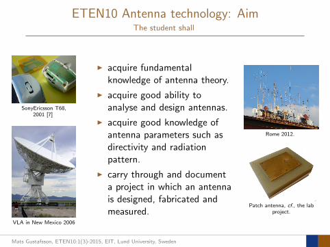
ETEN10 Antenna technology: AimThe student shall
SonyEricsson T68,2001 [7]
VLA in New Mexico 2006
I acquire fundamentalknowledge of antenna theory.
I acquire good ability toanalyse and design antennas.
I acquire good knowledge ofantenna parameters such asdirectivity and radiationpattern.
I carry through and documenta project in which an antennais designed, fabricated andmeasured.
Rome 2012.
Patch antenna, cf., the labproject.
Mats Gustafsson, ETEN10:1(3)-2015, EIT, Lund University, Sweden

Examination
In order to pass the course you must:
1. do all laboratory sessions
2. write a laboratory report (covering thelaboratory sessions)
3. do a written five hour examination (max60p, grade 3 for 30-39p, 4 for 40-49p, and 5for 50-60p).
Pass on the electronic quiz offers 5 bonus pointson the written exam in January 2016.Retake exams in April and August. Note, nobonus points on the retake exams.
Mats Gustafsson, ETEN10:1(4)-2015, EIT, Lund University, Sweden

Overview
I 2 lectures per week.
I 1 problem solving class (computer exercise)/week.
I 3 laboratory sessions.
I Electronic quiz (7 tests, 5p on the written exam inJanuary 2016).
I Written examination (max 60p, pass 30p).
I http://www.eit.lth.se/course/ETEN10
I Mats Gustafsson, Anders J. Johansson, DorukTayli, Zachary Miers
Mats Gustafsson, ETEN10:1(5)-2015, EIT, Lund University, Sweden
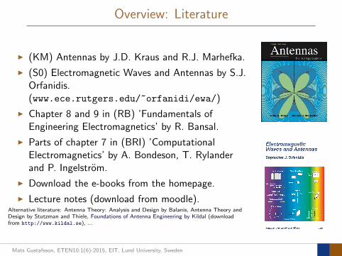
Overview: Literature
I (KM) Antennas by J.D. Kraus and R.J. Marhefka.
I (S0) Electromagnetic Waves and Antennas by S.J.Orfanidis.(www.ece.rutgers.edu/~orfanidi/ewa/)
I Chapter 8 and 9 in (RB) ’Fundamentals ofEngineering Electromagnetics’ by R. Bansal.
I Parts of chapter 7 in (BRI) ’ComputationalElectromagnetics’ by A. Bondeson, T. Rylanderand P. Ingelstrom.
I Download the e-books from the homepage.
I Lecture notes (download from moodle).Alternative literature: Antenna Theory: Analysis and Design by Balanis, Antenna Theory andDesign by Stutzman and Thiele, Foundations of Antenna Engineering by Kildal (downloadfrom http://www.kildal.se), ...
Mats Gustafsson, ETEN10:1(6)-2015, EIT, Lund University, Sweden

Schedule 2015
See homepage for details. Laboratory lessons preliminary for week3, 5, and 6, see the homepage.
Mats Gustafsson, ETEN10:1(7)-2015, EIT, Lund University, Sweden

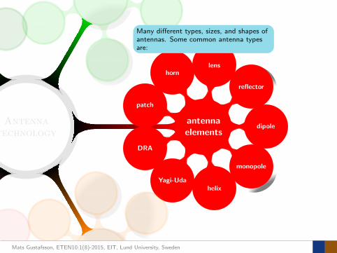
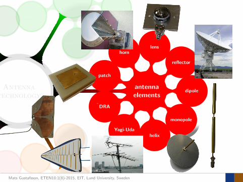
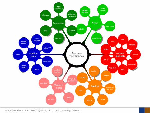
Antennatechnology
antennaelements
dipole
monopole
helixYagi-Uda
DRA
patch
hornlens
reflector
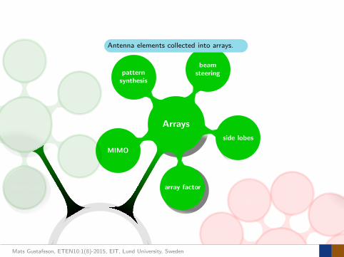
Arrays
beamsteering
side lobes
array factor
MIMO
patternsynthesis
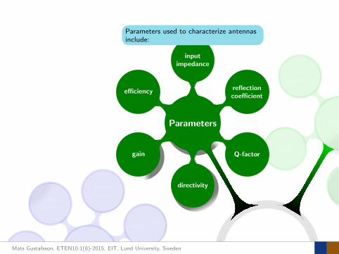
Parameters
directivity
gain
efficiency
inputimpedance
reflectioncoefficient
Q-factor
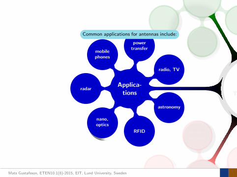
Applica-tions
radar
mobilephones
powertransfer
radio, TV
astronomy
RFID
nano,optics
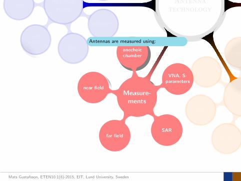
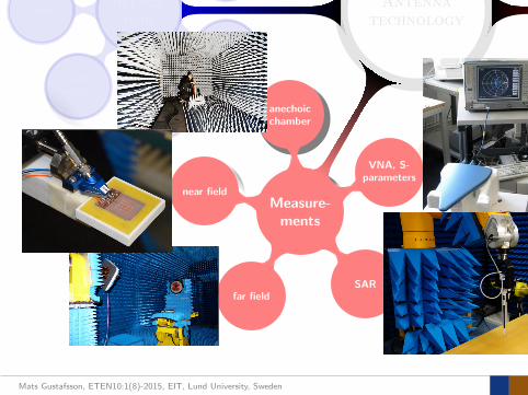
Measure-ments
far field
near field
anechoicchamber
VNA, S-parameters
SAR
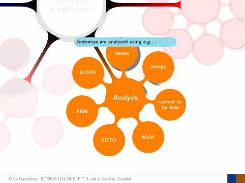
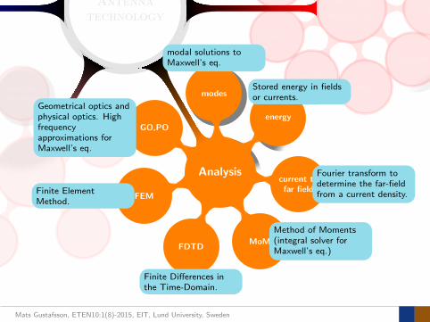
Analysis
MoMFDTD
FEM
GO,PO
modes
energy
current tofar field
Many different types, sizes, and shapes ofantennas. Some common antenna typesare:
Antenna elements collected into arrays.
0o
180o
90o
90o
45o
135o
45o
135o
−10−20−30dB
0o
180o
90o
90o
45o
135o
45o
135o
−10−20−30dB
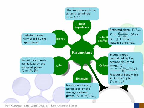
Parameters used to characterize antennasinclude:
Radiation intensitynormalized by theaccepted power.G = P/PT
Radiation intensitynormalized by theaverage radiatedpower. D = P/Pave
The impedance at theantenna terminalsZ = V/I
Reflected signal ΓUin,
Γ =Z−Z0Z+Z0
. Often
|Γ | ≤ 1/3 formatched antennas.
Stored energynormalized by theaverage dissipatedenergy Q =2ω maxWe,Wm
Pd.
Fractional bandwidthB ≈ 0.7/Q forΓ0 = 1/3.
Radiated powernormalized by theinput power.
Common applications for antennas include:
Antennas are measured using: Antennas are analyzed using e.g., :
Method of Moments(integral solver forMaxwell’s eq.)
Finite Differences inthe Time-Domain.
Finite ElementMethod.
Geometrical optics andphysical optics. Highfrequencyapproximations forMaxwell’s eq.
modal solutions toMaxwell’s eq.
Stored energy in fieldsor currents.
Fourier transform todetermine the far-fieldfrom a current density.
First three lectures:
I dipole antennas
I antenna parameters
I determine thefar-field from currentdistributions
I Method of momentsin the computerexercise
Mats Gustafsson, ETEN10:1(8)-2015, EIT, Lund University, Sweden
Antennatechnology
antennaelements
dipole
monopole
helixYagi-Uda
DRA
patch
hornlens
reflector
Arrays
beamsteering
side lobes
array factor
MIMO
patternsynthesis
Parameters
directivity
gain
efficiency
inputimpedance
reflectioncoefficient
Q-factor
Applica-tions
radar
mobilephones
powertransfer
radio, TV
astronomy
RFID
nano,optics
Measure-ments
far field
near field
anechoicchamber
VNA, S-parameters
SAR
Analysis
MoMFDTD
FEM
GO,PO
modes
energy
current tofar field
Many different types, sizes, and shapes ofantennas. Some common antenna typesare:
Antenna elements collected into arrays.
0o
180o
90o
90o
45o
135o
45o
135o
−10−20−30dB
0o
180o
90o
90o
45o
135o
45o
135o
−10−20−30dB
Parameters used to characterize antennasinclude:
Radiation intensitynormalized by theaccepted power.G = P/PT
Radiation intensitynormalized by theaverage radiatedpower. D = P/Pave
The impedance at theantenna terminalsZ = V/I
Reflected signal ΓUin,
Γ =Z−Z0Z+Z0
. Often
|Γ | ≤ 1/3 formatched antennas.
Stored energynormalized by theaverage dissipatedenergy Q =2ω maxWe,Wm
Pd.
Fractional bandwidthB ≈ 0.7/Q forΓ0 = 1/3.
Radiated powernormalized by theinput power.
Common applications for antennas include:
Antennas are measured using: Antennas are analyzed using e.g., :
Method of Moments(integral solver forMaxwell’s eq.)
Finite Differences inthe Time-Domain.
Finite ElementMethod.
Geometrical optics andphysical optics. Highfrequencyapproximations forMaxwell’s eq.
modal solutions toMaxwell’s eq.
Stored energy in fieldsor currents.
Fourier transform todetermine the far-fieldfrom a current density.
First three lectures:
I dipole antennas
I antenna parameters
I determine thefar-field from currentdistributions
I Method of momentsin the computerexercise
Mats Gustafsson, ETEN10:1(8)-2015, EIT, Lund University, Sweden
Antennatechnology
antennaelements
dipole
monopole
helixYagi-Uda
DRA
patch
hornlens
reflector
Arrays
beamsteering
side lobes
array factor
MIMO
patternsynthesis
Parameters
directivity
gain
efficiency
inputimpedance
reflectioncoefficient
Q-factor
Applica-tions
radar
mobilephones
powertransfer
radio, TV
astronomy
RFID
nano,optics
Measure-ments
far field
near field
anechoicchamber
VNA, S-parameters
SAR
Analysis
MoMFDTD
FEM
GO,PO
modes
energy
current tofar field
Many different types, sizes, and shapes ofantennas. Some common antenna typesare:
Antenna elements collected into arrays.
0o
180o
90o
90o
45o
135o
45o
135o
−10−20−30dB
0o
180o
90o
90o
45o
135o
45o
135o
−10−20−30dB
Parameters used to characterize antennasinclude:
Radiation intensitynormalized by theaccepted power.G = P/PT
Radiation intensitynormalized by theaverage radiatedpower. D = P/Pave
The impedance at theantenna terminalsZ = V/I
Reflected signal ΓUin,
Γ =Z−Z0Z+Z0
. Often
|Γ | ≤ 1/3 formatched antennas.
Stored energynormalized by theaverage dissipatedenergy Q =2ω maxWe,Wm
Pd.
Fractional bandwidthB ≈ 0.7/Q forΓ0 = 1/3.
Radiated powernormalized by theinput power.
Common applications for antennas include:
Antennas are measured using:
Antennas are analyzed using e.g., :
Method of Moments(integral solver forMaxwell’s eq.)
Finite Differences inthe Time-Domain.
Finite ElementMethod.
Geometrical optics andphysical optics. Highfrequencyapproximations forMaxwell’s eq.
modal solutions toMaxwell’s eq.
Stored energy in fieldsor currents.
Fourier transform todetermine the far-fieldfrom a current density.
First three lectures:
I dipole antennas
I antenna parameters
I determine thefar-field from currentdistributions
I Method of momentsin the computerexercise
Mats Gustafsson, ETEN10:1(8)-2015, EIT, Lund University, Sweden
Antennatechnology
antennaelements
dipole
monopole
helixYagi-Uda
DRA
patch
hornlens
reflector
Arrays
beamsteering
side lobes
array factor
MIMO
patternsynthesis
Parameters
directivity
gain
efficiency
inputimpedance
reflectioncoefficient
Q-factor
Applica-tions
radar
mobilephones
powertransfer
radio, TV
astronomy
RFID
nano,optics
Measure-ments
far field
near field
anechoicchamber
VNA, S-parameters
SAR
Analysis
MoMFDTD
FEM
GO,PO
modes
energy
current tofar field
Many different types, sizes, and shapes ofantennas. Some common antenna typesare:
Antenna elements collected into arrays.
0o
180o
90o
90o
45o
135o
45o
135o
−10−20−30dB
0o
180o
90o
90o
45o
135o
45o
135o
−10−20−30dB
Parameters used to characterize antennasinclude:
Radiation intensitynormalized by theaccepted power.G = P/PT
Radiation intensitynormalized by theaverage radiatedpower. D = P/Pave
The impedance at theantenna terminalsZ = V/I
Reflected signal ΓUin,
Γ =Z−Z0Z+Z0
. Often
|Γ | ≤ 1/3 formatched antennas.
Stored energynormalized by theaverage dissipatedenergy Q =2ω maxWe,Wm
Pd.
Fractional bandwidthB ≈ 0.7/Q forΓ0 = 1/3.
Radiated powernormalized by theinput power.
Common applications for antennas include:
Antennas are measured using: Antennas are analyzed using e.g., :
Method of Moments(integral solver forMaxwell’s eq.)
Finite Differences inthe Time-Domain.
Finite ElementMethod.
Geometrical optics andphysical optics. Highfrequencyapproximations forMaxwell’s eq.
modal solutions toMaxwell’s eq.
Stored energy in fieldsor currents.
Fourier transform todetermine the far-fieldfrom a current density.
First three lectures:
I dipole antennas
I antenna parameters
I determine thefar-field from currentdistributions
I Method of momentsin the computerexercise
Mats Gustafsson, ETEN10:1(8)-2015, EIT, Lund University, Sweden
Antennatechnology
antennaelements
dipole
monopole
helixYagi-Uda
DRA
patch
hornlens
reflector
Arrays
beamsteering
side lobes
array factor
MIMO
patternsynthesis
Parameters
directivity
gain
efficiency
inputimpedance
reflectioncoefficient
Q-factor
Applica-tions
radar
mobilephones
powertransfer
radio, TV
astronomy
RFID
nano,optics
Measure-ments
far field
near field
anechoicchamber
VNA, S-parameters
SAR
Analysis
MoMFDTD
FEM
GO,PO
modes
energy
current tofar field
Many different types, sizes, and shapes ofantennas. Some common antenna typesare:
Antenna elements collected into arrays.
0o
180o
90o
90o
45o
135o
45o
135o
−10−20−30dB
0o
180o
90o
90o
45o
135o
45o
135o
−10−20−30dB
Parameters used to characterize antennasinclude:
Radiation intensitynormalized by theaccepted power.G = P/PT
Radiation intensitynormalized by theaverage radiatedpower. D = P/Pave
The impedance at theantenna terminalsZ = V/I
Reflected signal ΓUin,
Γ =Z−Z0Z+Z0
. Often
|Γ | ≤ 1/3 formatched antennas.
Stored energynormalized by theaverage dissipatedenergy Q =2ω maxWe,Wm
Pd.
Fractional bandwidthB ≈ 0.7/Q forΓ0 = 1/3.
Radiated powernormalized by theinput power.
Common applications for antennas include:
Antennas are measured using: Antennas are analyzed using e.g., :
Method of Moments(integral solver forMaxwell’s eq.)
Finite Differences inthe Time-Domain.
Finite ElementMethod.
Geometrical optics andphysical optics. Highfrequencyapproximations forMaxwell’s eq.
modal solutions toMaxwell’s eq.
Stored energy in fieldsor currents.
Fourier transform todetermine the far-fieldfrom a current density.
First three lectures:
I dipole antennas
I antenna parameters
I determine thefar-field from currentdistributions
I Method of momentsin the computerexercise
Mats Gustafsson, ETEN10:1(8)-2015, EIT, Lund University, Sweden
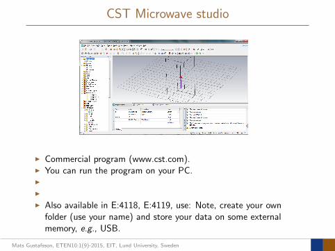
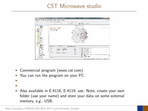
CST Microwave studio
I Commercial program (www.cst.com).I You can run the program on your PC.I
I
I Also available in E:4118, E:4119, use: Note, create your ownfolder (use your name) and store your data on some externalmemory, e.g., USB.
Mats Gustafsson, ETEN10:1(9)-2015, EIT, Lund University, Sweden
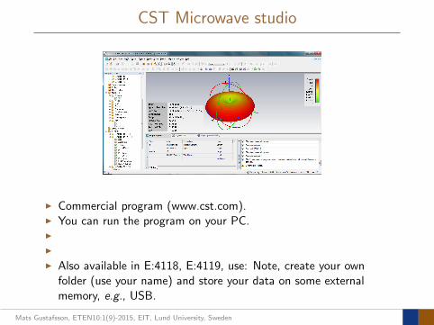
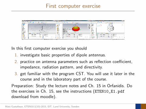
First computer exercise
In this first computer exercise you should
1. investigate basic properties of dipole antennas.
2. practice on antenna parameters such as reflection coefficient,impedance, radiation pattern, and directivity.
3. get familiar with the program CST. You will use it later in thecourse and in the laboratory part of the course.
Preparation: Study the lecture notes and Ch. 15 in Orfanidis. Dothe exercises in Ch. 15, see the instructions (ETEN10_E1.pdfdownload from moodle).
Mats Gustafsson, ETEN10:1(10)-2015, EIT, Lund University, Sweden
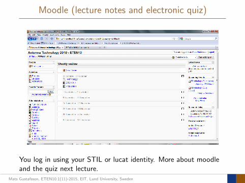
Moodle (lecture notes and electronic quiz)
You log in using your STIL or lucat identity. More about moodleand the quiz next lecture.
Mats Gustafsson, ETEN10:1(11)-2015, EIT, Lund University, Sweden
Moodle (lecture notes and electronic quiz)
You log in using your STIL or lucat identity. More about moodleand the quiz next lecture.
Mats Gustafsson, ETEN10:1(11)-2015, EIT, Lund University, Sweden
Moodle (lecture notes and electronic quiz)
You log in using your STIL or lucat identity. More about moodleand the quiz next lecture.
Mats Gustafsson, ETEN10:1(11)-2015, EIT, Lund University, Sweden
Outline
1 ETEN10 overview
2 Antenna background
3 Antenna parameters
Mats Gustafsson, ETEN10:1(12)-2015, EIT, Lund University, Sweden
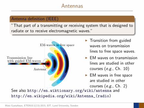
Antennas
Antenna definition (IEEE)
”That part of a transmitting or receiving system that is designed toradiate or to receive electromagnetic waves.”
Transmission line
Antenna
with guided EM-waves
EM-waves in free space
I Transition from guidedwaves on transmissionlines to free space waves.
I EM waves on transmissionlines are studied in othercourses (e.g., Ch. 10)
I EM waves in free spaceare studied in othercourses (e.g., Ch. 2)
See also http://en.wiktionary.org/wiki/antenna andhttp://en.wikipedia.org/wiki/Antenna_(radio)
Mats Gustafsson, ETEN10:1(13)-2015, EIT, Lund University, Sweden
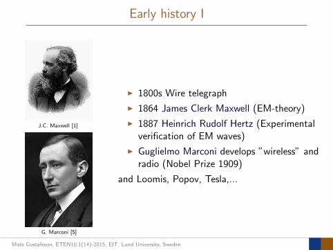
Early history I
J.C. Maxwell [1]
G. Marconi [5]
I 1800s Wire telegraph
I 1864 James Clerk Maxwell (EM-theory)
I 1887 Heinrich Rudolf Hertz (Experimentalverification of EM waves)
I Guglielmo Marconi develops ”wireless” andradio (Nobel Prize 1909)
and Loomis, Popov, Tesla,...
Mats Gustafsson, ETEN10:1(14)-2015, EIT, Lund University, Sweden

Early history II
Heinrich Rudolf Hertz [6]
I Heinrich Rudolf Hertz (1857–1894)
I Experimental verification of EM waves.
Hertz did not realize the practical importance ofhis experiments. He stated that,
”It’s of no use whatsoever[...] this is just an exper-iment that proves Maestro Maxwell was right - wejust have these mysterious electromagnetic wavesthat we cannot see with the naked eye. But theyare there.”
Asked about the ramifications of his discoveries,Hertz replied,
”Nothing, I guess.”
Mats Gustafsson, ETEN10:1(15)-2015, EIT, Lund University, Sweden
Applications
SonyEricsson T68, 2001
VLA in New Mexico [4]
RFID-TAG [3]
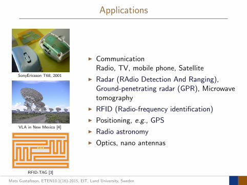
I CommunicationRadio, TV, mobile phone, Satellite
I Radar (RAdio Detection And Ranging),Ground-penetrating radar (GPR), Microwavetomography
I RFID (Radio-frequency identification)
I Positioning, e.g., GPS
I Radio astronomy
I Optics, nano antennas
Mats Gustafsson, ETEN10:1(16)-2015, EIT, Lund University, Sweden
Wireless communications
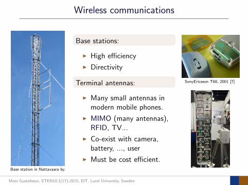
Base station in Nattavaara by.
Base stations:
I High efficiency
I Directivity
Terminal antennas:
I Many small antennas inmodern mobile phones.
I MIMO (many antennas),RFID, TV...
I Co-exist with camera,battery, ..., user
I Must be cost efficient.
SonyEricsson T68, 2001 [7]
Mats Gustafsson, ETEN10:1(17)-2015, EIT, Lund University, Sweden
Radio astronomy
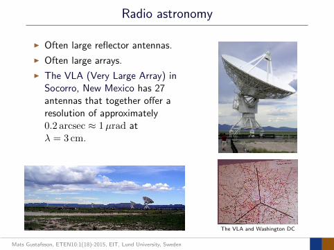
I Often large reflector antennas.
I Often large arrays.
I The VLA (Very Large Array) inSocorro, New Mexico has 27antennas that together offer aresolution of approximately0.2 arcsec ≈ 1µrad atλ = 3 cm.
The VLA and Washington DC
Mats Gustafsson, ETEN10:1(18)-2015, EIT, Lund University, Sweden
Outline
1 ETEN10 overview
2 Antenna background
3 Antenna parameters
Mats Gustafsson, ETEN10:1(19)-2015, EIT, Lund University, Sweden
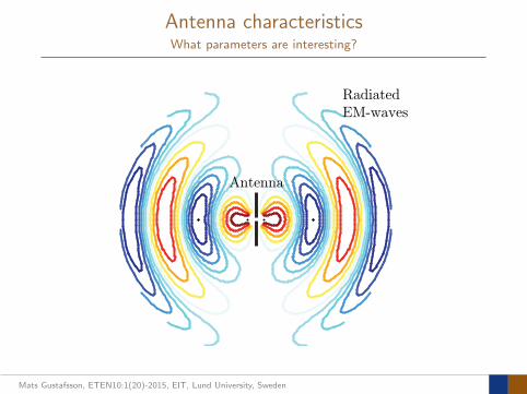
Antenna characteristicsWhat parameters are interesting?
Antenna
Radiated EM-waves
Mats Gustafsson, ETEN10:1(20)-2015, EIT, Lund University, Sweden
Antenna characteristics
V+
-I
J
Radiated EM-waves
Power flowin direction, µ,'
z
x
µ
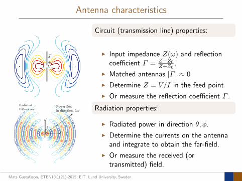
Circuit (transmission line) properties:
I Input impedance Z(ω) and reflectioncoefficient Γ = Z−Z0
Z+Z0.
I Matched antennas |Γ | ≈ 0
I Determine Z = V/I in the feed point
I Or measure the reflection coefficient Γ .
Radiation properties:
I Radiated power in direction θ, φ.
I Determine the currents on the antennaand integrate to obtain the far-field.
I Or measure the received (ortransmitted) field.
Mats Gustafsson, ETEN10:1(21)-2015, EIT, Lund University, Sweden
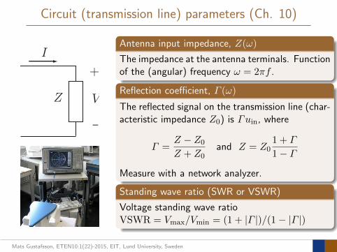
Circuit (transmission line) parameters (Ch. 10)
+
-
VZ
IAntenna input impedance, Z(ω)
The impedance at the antenna terminals. Functionof the (angular) frequency ω = 2πf .
Reflection coefficient, Γ (ω)
The reflected signal on the transmission line (char-acteristic impedance Z0) is Γuin, where
Γ =Z − Z0
Z + Z0and Z = Z0
1 + Γ
1− Γ
Measure with a network analyzer.
Standing wave ratio (SWR or VSWR)
Voltage standing wave ratioVSWR = Vmax/Vmin = (1 + |Γ |)/(1− |Γ |)
Mats Gustafsson, ETEN10:1(22)-2015, EIT, Lund University, Sweden

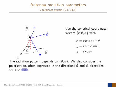
Antenna radiation parametersCoordinate system (Ch. 14.8)
x
y
z
φ
θ
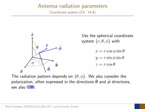
Use the spherical coordinatesystem r, θ, φ with
x = r cosφ sin θ
y = r sinφ sin θ
z = r cos θ
The radiation pattern depends on θ, φ. We also consider thepolarization, often expressed in the directions θ and φ directions,see also 39 .
Mats Gustafsson, ETEN10:1(23)-2015, EIT, Lund University, Sweden
Antenna radiation parametersCoordinate system (Ch. 14.8)
x
y
z
φ
θ
θ
φ
r Use the spherical coordinatesystem r, θ, φ with
x = r cosφ sin θ
y = r sinφ sin θ
z = r cos θ
The radiation pattern depends on θ, φ. We also consider thepolarization, often expressed in the directions θ and φ directions,see also 39 .
Mats Gustafsson, ETEN10:1(23)-2015, EIT, Lund University, Sweden
Antenna radiation parametersCoordinate system (Ch. 14.8)
x
y
z
φ
θ
θ
φr
Use the spherical coordinatesystem r, θ, φ with
x = r cosφ sin θ
y = r sinφ sin θ
z = r cos θ
The radiation pattern depends on θ, φ. We also consider thepolarization, often expressed in the directions θ and φ directions,see also 39 .
Mats Gustafsson, ETEN10:1(23)-2015, EIT, Lund University, Sweden
Latitude, longitude, and cardinal directions
Earth.
Radiated EM-waves
Power flowin direction, µ,'
z
x
µ
Radiated field.
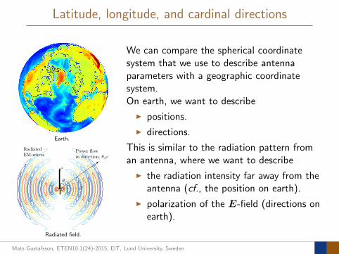
We can compare the spherical coordinatesystem that we use to describe antennaparameters with a geographic coordinatesystem.On earth, we want to describe
I positions.
I directions.
This is similar to the radiation pattern froman antenna, where we want to describe
I the radiation intensity far away from theantenna (cf., the position on earth).
I polarization of the E-field (directions onearth).
Mats Gustafsson, ETEN10:1(24)-2015, EIT, Lund University, Sweden

Latitude, longitude, and cardinal directions
Latitude and longitude on a sphere.Lund at 55N, 13E
longitude
latitude
−180−150−120 −90 −60 −30 0 30 60 90 120 150 180−90−75−60−45−30−150153045607590
Latitude and longitude in a Cartesiancoordinate system.
Use a set of coordinates that describepositions and directions on earth (here weneglect altitude).
I Latitude, angle between −90 (southpole) and 90 (north pole).
I Longitude, angle between −180 (west)and 180 (east) from the referencemeridian, 0 at Greenwich, UK.
I Directions: north (latitude) and east(longitude).
I Note the change of area close to thenorth and south poles.
Mats Gustafsson, ETEN10:1(25)-2015, EIT, Lund University, Sweden
Spherical coordinates for antennas
Á=0 Á=30
Á=60
Á=330
µ=0
µ=30
The θ, φ coordinate system on asphere.
Á0 30 60 90 120 150 180 210 240 270 300 330 360
0153045607590105120135150165180
µ
The θ, φ coordinate system.
Radiated EM-waves
Power flowin direction, µ,'
z
x
µ
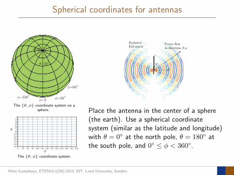
Place the antenna in the center of a sphere(the earth). Use a spherical coordinatesystem (similar as the latitude and longitude)with θ = 0 at the north pole, θ = 180 atthe south pole, and 0 ≤ φ < 360.
Mats Gustafsson, ETEN10:1(26)-2015, EIT, Lund University, Sweden
Spherical coordinates for antennas
Á
µµ
Á=0
Á
Á=30
Á=60
Á=330
µ=0
µ=30
Spherical coordinates, θ, φ, on a
sphere with the directions θ and φ.
Á0 30 60 90 120 150 180 210 240 270 300 330 360
0153045607590105120135150165180
µ
Á
µ
Á
µ
The θ, φ coordinate system.
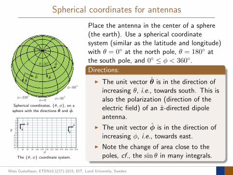
Place the antenna in the center of a sphere(the earth). Use a spherical coordinatesystem (similar as the latitude and longitude)with θ = 0 at the north pole, θ = 180 atthe south pole, and 0 ≤ φ < 360.
Directions:
I The unit vector θ is in the direction ofincreasing θ, i.e., towards south. This isalso the polarization (direction of theelectric field) of an z-directed dipoleantenna.
I The unit vector φ is in the direction ofincreasing φ, i.e., towards east.
I Note the change of area close to thepoles, cf., the sin θ in many integrals.
Mats Gustafsson, ETEN10:1(27)-2015, EIT, Lund University, Sweden
Spherical coordinate system
x
y
z
φ
θ
θ
φ
r
x
y
z
φ
θ
θ
φr
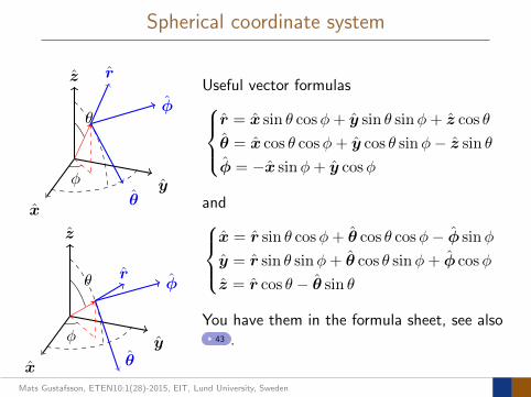
Useful vector formulasr = x sin θ cosφ+ y sin θ sinφ+ z cos θ
θ = x cos θ cosφ+ y cos θ sinφ− z sin θ
φ = −x sinφ+ y cosφ
andx = r sin θ cosφ+ θ cos θ cosφ− φ sinφ
y = r sin θ sinφ+ θ cos θ sinφ+ φ cosφ
z = r cos θ − θ sin θ
You have them in the formula sheet, see also43 .
Mats Gustafsson, ETEN10:1(28)-2015, EIT, Lund University, Sweden
Antenna radiation parameters (Ch. 15.2)
VV1
y
x
z
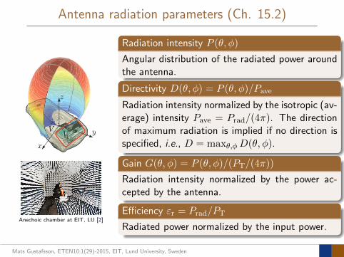
Anechoic chamber at EIT, LU [2]
Radiation intensity P (θ, φ)
Angular distribution of the radiated power aroundthe antenna.
Directivity D(θ, φ) = P (θ, φ)/Pave
Radiation intensity normalized by the isotropic (av-erage) intensity Pave = Prad/(4π). The directionof maximum radiation is implied if no direction isspecified, i.e., D = maxθ,φD(θ, φ).
Gain G(θ, φ) = P (θ, φ)/(PT/(4π))
Radiation intensity normalized by the power ac-cepted by the antenna.
Efficiency εr = Prad/PT
Radiated power normalized by the input power.
Mats Gustafsson, ETEN10:1(29)-2015, EIT, Lund University, Sweden
Electromagnetic fields
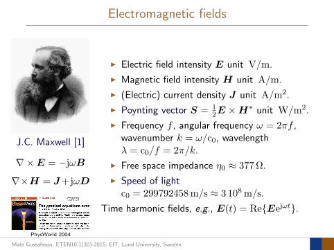
J.C. Maxwell [1]
∇×E = −jωB
∇×H = J+jωD
PhysWorld 2004
I Electric field intensity E unit V/m.
I Magnetic field intensity H unit A/m.
I (Electric) current density J unit A/m2.
I Poynting vector S = 12E ×H
∗ unit W/m2.
I Frequency f , angular frequency ω = 2πf ,wavenumber k = ω/c0, wavelengthλ = c0/f = 2π/k.
I Free space impedance η0 ≈ 377 Ω.
I Speed of lightc0 = 299792458 m/s ≈ 3 108 m/s.
Time harmonic fields, e.g., E(t) = ReEejωt.
Mats Gustafsson, ETEN10:1(30)-2015, EIT, Lund University, Sweden
Current to radiation pattern I
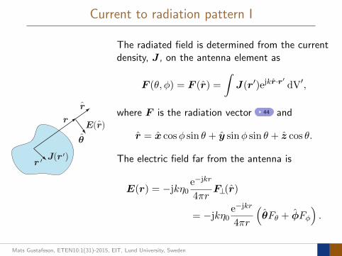
J(r )
E(r)
r
µ
^
^r
0
r 0
The radiated field is determined from the currentdensity, J , on the antenna element as
F (θ, φ) = F (r) =
∫J(r′)ejkr·r
′dV′,
where F is the radiation vector 44 and
r = x cosφ sin θ + y sinφ sin θ + z cos θ.
The electric field far from the antenna is
E(r) = −jkη0e−jkr
4πrF⊥(r)
= −jkη0e−jkr
4πr
(θFθ + φFφ
).
Mats Gustafsson, ETEN10:1(31)-2015, EIT, Lund University, Sweden
Current to radiation pattern II
VV1
y
x
z
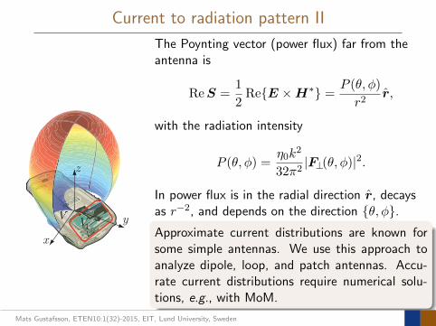
The Poynting vector (power flux) far from theantenna is
ReS =1
2ReE ×H∗ =
P (θ, φ)
r2r,
with the radiation intensity
P (θ, φ) =η0k
2
32π2|F⊥(θ, φ)|2.
In power flux is in the radial direction r, decaysas r−2, and depends on the direction θ, φ.Approximate current distributions are known forsome simple antennas. We use this approach toanalyze dipole, loop, and patch antennas. Accu-rate current distributions require numerical solu-tions, e.g., with MoM.
Mats Gustafsson, ETEN10:1(32)-2015, EIT, Lund University, Sweden
Near field and far field
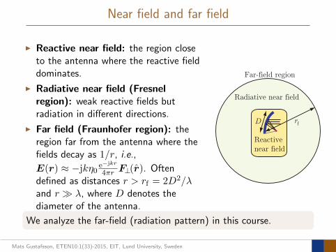
I Reactive near field: the region closeto the antenna where the reactive fielddominates.
I Radiative near field (Fresnelregion): weak reactive fields butradiation in different directions.
I Far field (Fraunhofer region): theregion far from the antenna where thefields decay as 1/r, i.e.,
E(r) ≈ −jkη0e−jkr
4πr F⊥(r). Oftendefined as distances r > rf = 2D2/λand r λ, where D denotes thediameter of the antenna.
Far-field region
Radiative near field
Reactive near field
D rf
We analyze the far-field (radiation pattern) in this course.
Mats Gustafsson, ETEN10:1(33)-2015, EIT, Lund University, Sweden
Receiving antenna parameters
Z0
E
k
in
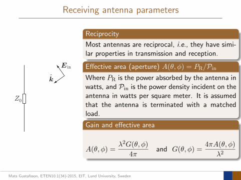
Reciprocity
Most antennas are reciprocal, i.e., they have simi-lar properties in transmission and reception.
Effective area (aperture) A(θ, φ) = PR/PinWhere PR is the power absorbed by the antenna inwatts, and Pin is the power density incident on theantenna in watts per square meter. It is assumedthat the antenna is terminated with a matchedload.
Gain and effective area
A(θ, φ) =λ2G(θ, φ)
4πand G(θ, φ) =
4πA(θ, φ)
λ2
Mats Gustafsson, ETEN10:1(34)-2015, EIT, Lund University, Sweden
Friis transmission equation
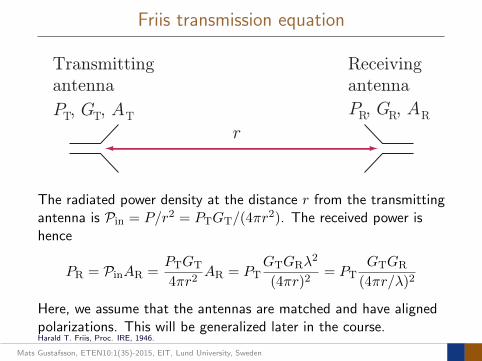
Transmitting
antenna
Receiving
antenna
r
P , G , ATTTP , G , ARRR
The radiated power density at the distance r from the transmittingantenna is Pin = P/r2 = PTGT/(4πr
2). The received power ishence
PR = PinAR =PTGT
4πr2AR = PT
GTGRλ2
(4πr)2= PT
GTGR
(4πr/λ)2
Here, we assume that the antennas are matched and have alignedpolarizations. This will be generalized later in the course.Harald T. Friis, Proc. IRE, 1946.
Mats Gustafsson, ETEN10:1(35)-2015, EIT, Lund University, Sweden
Next lecture
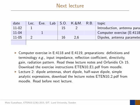
date Lec. Exe. Lab S.O. K.&M. R.B. topic11-02 1 15 2 Introduction, antenna parameters11-04 1 Computer exercise (E:4118, E:4119)11-05 2 16 2,6 Dipoles, antenna parameters, MoM
I Computer exercise in E:4118 and E:4119, preparations: definitions andterminology e.g., input impedance, reflection coefficient, directivity,gain, radiation pattern. Read these lecture notes and Orfanidis Ch 15.Download the exercise instructions ETEN10 E1.pdf from moodle.
I Lecture 2: dipole antennas, short dipole, half-wave dipole, simpleanalytic expressions, download the lecture notes ETEN10 2.pdf frommoodle. Read before next lecture.
Mats Gustafsson, ETEN10:1(36)-2015, EIT, Lund University, Sweden
References
[1] James Clerk Maxwell. http://en.wikipedia.org/.
[2] The anechoic chamber at EIT, LU, 2002. LTH-Nytt.
[3] RFID TAG, 2008. http://en.wikipedia.org/.
[4] Hajor. The Very Large Array at Socorro, New Mexico, US,2004. http://en.wikipedia.org/.
[5] Nobel foundation. Marconi, 1909. http://nobelprize.org/.
[6] Oliver Heaviside: Sage in Solitude. Heinrich Rudolf Hertz,1894. http://en.wikipedia.org/.
[7] Sony Ericsson. T68, 2001.
Mats Gustafsson, ETEN10:1(37)-2015, EIT, Lund University, Sweden
Outline
4 Appendix: Additional materialVectorsPotentials and far fields
Mats Gustafsson, ETEN10:1(38)-2015, EIT, Lund University, Sweden
Appendix: vectors
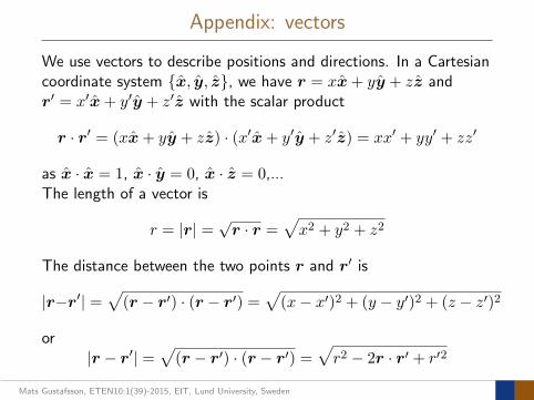
We use vectors to describe positions and directions. In a Cartesiancoordinate system x, y, z, we have r = xx+ yy + zz andr′ = x′x+ y′y + z′z with the scalar product
r · r′ = (xx+ yy + zz) · (x′x+ y′y + z′z) = xx′ + yy′ + zz′
as x · x = 1, x · y = 0, x · z = 0,...The length of a vector is
r = |r| =√r · r =
√x2 + y2 + z2
The distance between the two points r and r′ is
|r−r′| =√
(r − r′) · (r − r′) =√
(x− x′)2 + (y − y′)2 + (z − z′)2
or|r − r′| =
√(r − r′) · (r − r′) =
√r2 − 2r · r′ + r′2
Mats Gustafsson, ETEN10:1(39)-2015, EIT, Lund University, Sweden
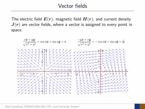
Vector fields
The electric field E(r), magnetic field H(r), and current densityJ(r) are vector fields, where a vector is assigned to every point inspace.
−2 −1 1 2
−2
−1
1
2
x
y
xx+ yy√x2 + y2
= cosφx+ sinφy = r
−2 −1 1 2
−2
−1
1
2
x
y
−yx+ xy√x2 + y2
= − cosφx+ sinφy = φ
Mats Gustafsson, ETEN10:1(40)-2015, EIT, Lund University, Sweden
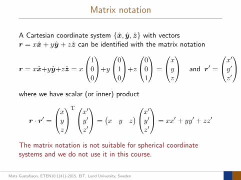
Matrix notation
A Cartesian coordinate system x, y, z with vectorsr = xx+ yy + zz can be identified with the matrix notation
r = xx+yy+zz = x
100
+y
010
+z
001
=
xyz
and r′ =
x′y′z′
where we have scalar (or inner) product
r · r′ =
xyz
Tx′y′z′
=(x y z
)x′y′z′
= xx′ + yy′ + zz′
The matrix notation is not suitable for spherical coordinatesystems and we do not use it in this course.
Mats Gustafsson, ETEN10:1(41)-2015, EIT, Lund University, Sweden

Spherical coordinate system
x
y
z
r
φ
θ
x
y
z
r
φ
θ
A vector r = xx+ yy + zz can be described ina spherical coordinate system r, θ, φ
x = r cosφ sin θ
y = r sinφ sin θ
z = r cos θ
I r = |r| =√x2 + y2 + z2 is the length of r
(the distance from the center of thecoordinate system to the point r).
I θ is the polar angle, i.e., the angle from zto r.
I φ is the azimuthal angle, i.e., the angle fromx to the projection of r in the xy-plane.
Mats Gustafsson, ETEN10:1(42)-2015, EIT, Lund University, Sweden
Spherical coordinate system
x
y
z
φ
θ
θ
φ
r
x
y
z
φ
θ
θ
φr
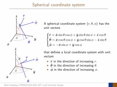
A spherical coordinate system r, θ, φ has theunit vectors
r = x sin θ cosφ+ y sin θ sinφ+ z cos θ
θ = x cos θ cosφ+ y cos θ sinφ− z sin θ
φ = −x sinφ+ y cosφ
that defines a local coordinate system with unitvectors
I r in the direction of increasing r.I θ in the direction of increasing θ.I φ in the direction of increasing φ.
Mats Gustafsson, ETEN10:1(43)-2015, EIT, Lund University, Sweden
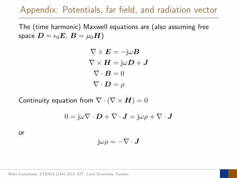
Appendix: Potentials, far field, and radiation vector
The (time harmonic) Maxwell equations are (also assuming freespace D = ε0E, B = µ0H)
∇×E = −jωB
∇×H = jωD + J
∇ ·B = 0
∇ ·D = ρ
Continuity equation from ∇ · (∇×H) = 0
0 = jω∇ ·D +∇ · J = jωρ+∇ · J
orjωρ = −∇ · J
Mats Gustafsson, ETEN10:1(44)-2015, EIT, Lund University, Sweden
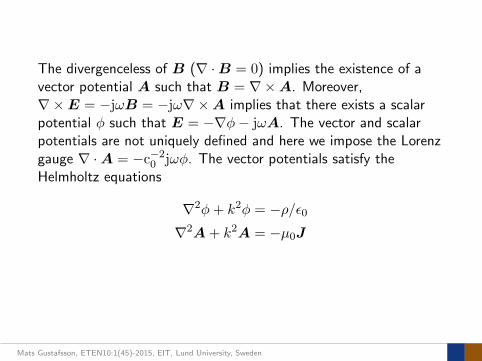
The divergenceless of B (∇ ·B = 0) implies the existence of avector potential A such that B = ∇×A. Moreover,∇×E = −jωB = −jω∇×A implies that there exists a scalarpotential φ such that E = −∇φ− jωA. The vector and scalarpotentials are not uniquely defined and here we impose the Lorenzgauge ∇ ·A = −c−20 jωφ. The vector potentials satisfy theHelmholtz equations
∇2φ+ k2φ = −ρ/ε0∇2A+ k2A = −µ0J
Mats Gustafsson, ETEN10:1(45)-2015, EIT, Lund University, Sweden
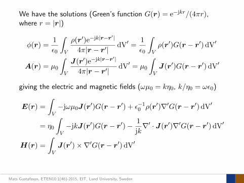
We have the solutions (Green’s function G(r) = e−jkr/(4πr),where r = |r|)
φ(r) =1
ε0
∫V
ρ(r′)e−jk|r−r′|
4π|r − r′|dV′ =
1
ε0
∫Vρ(r′)G(r − r′) dV′
A(r) = µ0
∫V
J(r′)e−jk|r−r′|
4π|r − r′|dV′ = µ0
∫VJ(r′)G(r − r′) dV′
giving the electric and magnetic fields (ωµ0 = kη0, k/η0 = ωε0)
E(r) =
∫V−jωµ0J(r′)G(r − r′) + ε−10 ρ(r′)∇′G(r − r′) dV′
= η0
∫V−jkJ(r′)G(r − r′)− 1
jk∇′ · J(r′)∇′G(r − r′) dV′
H(r) =
∫VJ(r′)×∇′G(r − r′) dV′
Mats Gustafsson, ETEN10:1(46)-2015, EIT, Lund University, Sweden
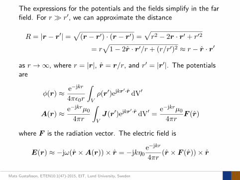
The expressions for the potentials and the fields simplify in the farfield. For r r′, we can approximate the distance
R = |r − r′| =√
(r − r′) · (r − r′) =√r2 − 2r · r′ + r′2
= r√
1− 2r · r′/r + (r/r′)2 ≈ r − r · r′
as r →∞, where r = |r|, r = r/r, and r′ = |r′|. The potentialsare
φ(r) ≈ e−jkr
4πε0r
∫Vρ(r′)ejkr
′·r dV′
A(r) ≈ e−jkrµ04πr
∫VJ(r′)ejkr
′·r dV′ =e−jkrµ0
4πrF (r)
where F is the radiation vector. The electric field is
E(r) ≈ −jω(r ×A(r))× r = −jkη0e−jkr
4πr(r × F (r))× r
Mats Gustafsson, ETEN10:1(47)-2015, EIT, Lund University, Sweden


![Antenna design for Sigfox Ready devices - iSMAC-NC · 2018-01-13 · [REF3] Antenna Theory, Analysis and Design, second edition, C. A. Balanis. [REF4] Metamaterial-Inspired Efficient](https://static.documents.pub/doc/80x56/5e893bd7f341654e79323165/antenna-design-for-sigfox-ready-devices-ismac-nc-2018-01-13-ref3-antenna-theory.jpg)

![Antenna Theory, Analysis and Design (4e) by Balanis)]](https://static.documents.pub/doc/80x56/61edd62e1af1993c6d6ea6e1/antenna-theory-analysis-and-design-4e-by-balanis.jpg)
![Solution Manual Antenna Theory by Balanis Edition2 Chapter13b[1]](https://static.documents.pub/doc/80x56/547fd9625806b5c75e8b4940/solution-manual-antenna-theory-by-balanis-edition2-chapter13b1.jpg)
