149
ETSI TS 103 634 V1.1.1 (2019-08) Digital Enhanced Cordless Telecommunications (DECT); Low Complexity Communication Codec plus (LC3plus) TECHNICAL SPECIFICATION
ETSI TS 103 634 V1.1.1 (2019-08)
Digital Enhanced Cordless Telecommunications (DECT); Low Complexity Communication Codec plus (LC3plus)
TECHNICAL SPECIFICATION
ETSI
ETSI TS 103 634 V1.1.1 (2019-08)2
Reference DTS/DECT-00338
Keywords audio, codec, DECT, Full-Band, LC3plus,
superwideband, voice, VoIP
ETSI
650 Route des Lucioles F-06921 Sophia Antipolis Cedex - FRANCE
Tel.: +33 4 92 94 42 00 Fax: +33 4 93 65 47 16
Siret N° 348 623 562 00017 - NAF 742 C
Association à but non lucratif enregistrée à la Sous-Préfecture de Grasse (06) N° 7803/88
Important notice
The present document can be downloaded from: http://www.etsi.org/standards-search
The present document may be made available in electronic versions and/or in print. The content of any electronic and/or print versions of the present document shall not be modified without the prior written authorization of ETSI. In case of any
existing or perceived difference in contents between such versions and/or in print, the prevailing version of an ETSI deliverable is the one made publicly available in PDF format at www.etsi.org/deliver.
Users of the present document should be aware that the document may be subject to revision or change of status. Information on the current status of this and other ETSI documents is available at
https://portal.etsi.org/TB/ETSIDeliverableStatus.aspx
If you find errors in the present document, please send your comment to one of the following services: https://portal.etsi.org/People/CommiteeSupportStaff.aspx
Copyright Notification
No part may be reproduced or utilized in any form or by any means, electronic or mechanical, including photocopying and microfilm except as authorized by written permission of ETSI.
The content of the PDF version shall not be modified without the written authorization of ETSI. The copyright and the foregoing restriction extend to reproduction in all media.
© ETSI 2019.
All rights reserved.
DECT™, PLUGTESTS™, UMTS™ and the ETSI logo are trademarks of ETSI registered for the benefit of its Members. 3GPP™ and LTE™ are trademarks of ETSI registered for the benefit of its Members and
of the 3GPP Organizational Partners. oneM2M™ logo is a trademark of ETSI registered for the benefit of its Members and
of the oneM2M Partners. GSM® and the GSM logo are trademarks registered and owned by the GSM Association.
ETSI
ETSI TS 103 634 V1.1.1 (2019-08)3
Contents Intellectual Property Rights ................................................................................................................................ 9
Foreword ............................................................................................................................................................. 9
Modal verbs terminology .................................................................................................................................... 9
Executive summary ............................................................................................................................................ 9
Introduction ...................................................................................................................................................... 10
1 Scope ...................................................................................................................................................... 11
2 References .............................................................................................................................................. 11
2.1 Normative references ....................................................................................................................................... 11
2.2 Informative references ...................................................................................................................................... 12
3 Definition of terms, symbols and abbreviations ..................................................................................... 13
3.1 Terms ................................................................................................................................................................ 13
3.2 Symbols ............................................................................................................................................................ 14
3.2.1 Mathematical symbols ................................................................................................................................ 14
3.2.2 Operator symbols ........................................................................................................................................ 14
3.3 Abbreviations ................................................................................................................................................... 14
4 General description................................................................................................................................. 16
4.1 Overview .......................................................................................................................................................... 16
4.2 Transcoding functions ...................................................................................................................................... 17
4.3 ANSI C-code .................................................................................................................................................... 19
4.4 Conformance testing......................................................................................................................................... 19
4.5 RTP payload format ......................................................................................................................................... 20
4.6 Performance characterization ........................................................................................................................... 20
5 Codec algorithm description .................................................................................................................. 20
5.1 General codec description ................................................................................................................................ 20
5.2 General codec parameters................................................................................................................................. 21
5.2.1 Audio channels ........................................................................................................................................... 21
5.2.2 Sampling rates ............................................................................................................................................ 21
5.2.3 Bits per sample ........................................................................................................................................... 21
5.2.4 Frame size and delay................................................................................................................................... 21
5.2.5 Bit budget and bitrate .................................................................................................................................. 22
5.3 Encoding process .............................................................................................................................................. 22
5.3.1 Encoder modules ........................................................................................................................................ 22
5.3.2 Input signal ................................................................................................................................................. 23
5.3.3 Input signal scaling ..................................................................................................................................... 23
5.3.4 Low delay MDCT analysis ......................................................................................................................... 23
5.3.4.1 Overview ............................................................................................................................................... 23
5.3.4.2 Update time buffer ................................................................................................................................ 24
5.3.4.3 Time-frequency transformation............................................................................................................. 24
5.3.4.4 Energy estimation per band ................................................................................................................... 25
5.3.5 Bandwidth detector ..................................................................................................................................... 25
5.3.5.1 Algorithm .............................................................................................................................................. 25
5.3.5.2 Parameters ............................................................................................................................................. 26
5.3.6 Time Domain Attack Detector .................................................................................................................... 26
5.3.6.1 Overview ............................................................................................................................................... 26
5.3.6.2 Downsampling and Filtering of Input Signal ........................................................................................ 27
5.3.6.3 Energy Calculation ................................................................................................................................ 27
5.3.6.4 Attack Detection ................................................................................................................................... 27
5.3.7 Spectral Noise Shaping ............................................................................................................................... 27
5.3.7.1 Overview ............................................................................................................................................... 27
5.3.7.2 SNS analysis ......................................................................................................................................... 28
5.3.7.2.1 Overview ......................................................................................................................................... 28
5.3.7.2.2 Padding ............................................................................................................................................ 28
5.3.7.2.3 Smoothing ....................................................................................................................................... 28
ETSI
ETSI TS 103 634 V1.1.1 (2019-08)4
5.3.7.2.4 Pre-emphasis ................................................................................................................................... 29
5.3.7.2.5 Noise floor ....................................................................................................................................... 29
5.3.7.2.6 Logarithm ........................................................................................................................................ 29
5.3.7.2.7 Band Energy Grouping .................................................................................................................... 29
5.3.7.2.8 Mean removal and scaling, attack handling..................................................................................... 29
5.3.7.3 SNS quantization ................................................................................................................................... 30
5.3.7.3.1 General ............................................................................................................................................ 30
5.3.7.3.2 Stage 1 ............................................................................................................................................. 31
5.3.7.3.3 Stage 2 ............................................................................................................................................. 31
5.3.7.3.3.1 General ....................................................................................................................................... 31
5.3.7.3.3.2 Transform .................................................................................................................................. 31
5.3.7.3.3.3 Stage 2 Target Preparation ......................................................................................................... 32
5.3.7.3.3.4 Shape Candidates ....................................................................................................................... 32
5.3.7.3.3.5 Stage 2 Shape Search ................................................................................................................. 32
5.3.7.3.3.6 Adjustment Gain Candidates ..................................................................................................... 34
5.3.7.3.3.7 Shape and Gain combination determination .............................................................................. 35
5.3.7.3.3.8 Enumeration of the selected PVQ pulse configurations ............................................................. 35
5.3.7.3.4 Multiplexing of SNS VQ Codewords .............................................................................................. 36
5.3.7.3.5 Synthesis of the Quantized SNS scale factor vector ........................................................................ 38
5.3.7.4 SNS scale factors interpolation ............................................................................................................. 38
5.3.7.5 Spectral shaping .................................................................................................................................... 39
5.3.8 Bandwidth control ...................................................................................................................................... 39
5.3.9 Temporal noise shaping (TNS) ................................................................................................................... 39
5.3.9.1 Overview ............................................................................................................................................... 39
5.3.9.2 TNS analysis ......................................................................................................................................... 40
5.3.9.3 Quantization .......................................................................................................................................... 41
5.3.9.4 Filtering ................................................................................................................................................. 42
5.3.10 Long term postfilter .................................................................................................................................... 42
5.3.10.1 Overview ............................................................................................................................................... 42
5.3.10.2 Time-domain signals ............................................................................................................................. 43
5.3.10.3 Resampling............................................................................................................................................ 43
5.3.10.4 High-pass filtering ................................................................................................................................. 43
5.3.10.5 Pitch detection algorithm ...................................................................................................................... 43
5.3.10.6 LTPF bitstream ..................................................................................................................................... 44
5.3.10.7 LTPF pitch-lag parameter ..................................................................................................................... 45
5.3.10.8 LTPF activation bit ............................................................................................................................... 45
5.3.11 Spectral quantization................................................................................................................................... 46
5.3.11.1 Overview ............................................................................................................................................... 46
5.3.11.2 Bit budget .............................................................................................................................................. 46
5.3.11.3 First global gain estimation ................................................................................................................... 46
5.3.11.4 Quantization .......................................................................................................................................... 48
5.3.11.5 Bit consumption .................................................................................................................................... 48
5.3.11.6 Truncation ............................................................................................................................................. 49
5.3.11.7 Global gain adjustment ......................................................................................................................... 50
5.3.12 Residual coding .......................................................................................................................................... 50
5.3.13 Noise level estimation ................................................................................................................................. 51
5.3.13.1 Overview ............................................................................................................................................... 51
5.3.13.2 Relevant spectral lines ........................................................................................................................... 51
5.3.13.3 Noise level calculation .......................................................................................................................... 52
5.3.14 Bitstream encoding ..................................................................................................................................... 52
5.3.14.1 Overview ............................................................................................................................................... 52
5.3.14.2 Initialization .......................................................................................................................................... 52
5.3.14.3 Side information .................................................................................................................................... 53
5.3.14.4 Arithmetic encoding .............................................................................................................................. 53
5.3.14.4.1 Overview ......................................................................................................................................... 53
5.3.14.4.2 Pseudo code implementation ........................................................................................................... 54
5.3.14.5 Residual data and finalization ............................................................................................................... 55
5.3.14.6 Functions ............................................................................................................................................... 56
5.4 Decoding process ............................................................................................................................................. 58
5.4.1 Decoder modules ........................................................................................................................................ 58
5.4.2 Bitstream decoding ..................................................................................................................................... 58
ETSI
ETSI TS 103 634 V1.1.1 (2019-08)5
5.4.2.1 Overview ............................................................................................................................................... 58
5.4.2.2 Initialization .......................................................................................................................................... 59
5.4.2.3 Side information .................................................................................................................................... 59
5.4.2.4 Special decoder mode indicators ........................................................................................................... 60
5.4.2.5 Padding pattern ..................................................................................................................................... 60
5.4.2.6 Bandwidth interpretation ....................................................................................................................... 61
5.4.2.7 Arithmetic decoding .............................................................................................................................. 61
5.4.2.8 Residual data and finalization ............................................................................................................... 62
5.4.2.9 Functions ............................................................................................................................................... 64
5.4.3 Residual decoding ....................................................................................................................................... 65
5.4.4 Noise filling ................................................................................................................................................ 65
5.4.5 Global gain.................................................................................................................................................. 66
5.4.6 TNS decoder ............................................................................................................................................... 66
5.4.7 SNS decoder ............................................................................................................................................... 67
5.4.7.1 Overview ............................................................................................................................................... 67
5.4.7.2 SNS scale factor decoding .................................................................................................................... 67
5.4.7.2.1 SNS VQ decoding ........................................................................................................................... 67
5.4.7.2.2 Stage 1 SNS VQ decoding............................................................................................................... 68
5.4.7.2.3 Stage 2 SNS VQ decoding............................................................................................................... 68
5.4.7.2.3.1 Stage 2 SNS-VQ index demultiplexing ..................................................................................... 68
5.4.7.2.3.2 De-enumeration of the shape indices ......................................................................................... 69
5.4.7.2.4 Unit energy normalization of the received shape ............................................................................ 71
5.4.7.2.5 Reconstruction of the Quantized SNS Scalefactors ......................................................................... 71
5.4.7.3 SNS scale factors interpolation ............................................................................................................. 71
5.4.7.4 Spectral Shaping ................................................................................................................................... 72
5.4.8 Low delay MDCT synthesis ....................................................................................................................... 72
5.4.9 Long term postfilter .................................................................................................................................... 73
5.4.9.1 Overview ............................................................................................................................................... 73
5.4.9.2 Transition handling ............................................................................................................................... 73
5.4.9.3 Remaining of the frame ......................................................................................................................... 74
5.4.10 Output signal scaling and rounding ............................................................................................................ 76
5.5 Frame structure ................................................................................................................................................. 76
5.6 Error concealment ............................................................................................................................................ 76
5.6.1 General consideration ................................................................................................................................. 76
5.6.2 PLC trigger ................................................................................................................................................. 77
5.6.3 PLC method selection and method application ........................................................................................... 77
5.6.3.1 Method selection ................................................................................................................................... 77
5.6.3.2 MDCT frame repetition with sign scrambling ...................................................................................... 78
5.6.3.3 Time domain concealment .................................................................................................................... 80
5.6.3.3.1 Overview ......................................................................................................................................... 80
5.6.3.3.2 LPC parameter calculation .............................................................................................................. 80
5.6.3.3.3 Construction of the periodic part of the excitation .......................................................................... 81
5.6.3.3.4 Construction of the random part of the excitation ........................................................................... 82
5.6.3.3.5 Construction of the total excitation, synthesis and post-processing ................................................ 83
5.6.3.3.6 Time domain alias cancelation ........................................................................................................ 84
5.6.3.3.7 Handling of multiple frame losses ................................................................................................... 84
5.6.3.4 Frequency domain concealment (Phase ECU) ...................................................................................... 85
5.6.3.4.1 Phase ECU overview ....................................................................................................................... 85
5.6.3.4.2 Spectral Shape ................................................................................................................................. 85
5.6.3.4.3 Transient analysis ............................................................................................................................ 86
5.6.3.4.4 Fine Spectral analysis ...................................................................................................................... 87
5.6.3.4.5 Frame reconstruction ....................................................................................................................... 88
5.6.4 PLC operation related to LTPF ................................................................................................................... 90
5.7 External rate adaptation .................................................................................................................................... 90
5.8 High-resolution audio support .......................................................................................................................... 90
5.8.1 Overview .................................................................................................................................................... 90
5.8.2 Changes to the algorithm in high-resolution mode ..................................................................................... 90
5.9 Tables and constants ......................................................................................................................................... 93
5.9.1 Band tables index ........................................................................................................................................ 93
5.9.2 Low delay MDCT windows........................................................................................................................ 93
5.9.2.1 Frame size 2,5 ms .................................................................................................................................. 93

ETSI
ETSI TS 103 634 V1.1.1 (2019-08)6
5.9.2.2 Frame size 5 ms ..................................................................................................................................... 94
5.9.2.3 Frame size 10 ms ................................................................................................................................... 94
5.9.3 SNS quantization ........................................................................................................................................ 94
5.9.4 Temporal noise shaping .............................................................................................................................. 96
5.9.5 Long term postfiltering ............................................................................................................................... 96
5.9.6 Spectral data................................................................................................................................................ 96
6 Source code description.......................................................................................................................... 97
6.1 Overview .......................................................................................................................................................... 97
6.2 Contents of the C source code .......................................................................................................................... 97
6.3 File formats ...................................................................................................................................................... 97
6.3.1 Sound file (encoder input and decoder output) ........................................................................................... 97
6.3.2 Switching profile (encoder input) ............................................................................................................... 98
6.3.3 Parameter bitstream file (encoder output and decoder input) ..................................................................... 98
6.4 Test vector package .......................................................................................................................................... 98
7 Conformance .......................................................................................................................................... 98
7.1 Overview .......................................................................................................................................................... 98
7.2 Test framework ................................................................................................................................................ 99
7.2.1 Test material ............................................................................................................................................... 99
7.2.2 Test permutations and codec parameters .................................................................................................... 99
7.2.3 Modules under test ...................................................................................................................................... 99
7.2.4 Quality metric calculation ......................................................................................................................... 100
7.2.4.1 Root Mean Square ............................................................................................................................... 100
7.2.4.2 Delta ODG value ................................................................................................................................. 101
7.2.4.3 Maximum loudness difference (MLD)................................................................................................ 101
7.2.4.4 Thresholds ........................................................................................................................................... 102
7.2.5 Software and tools .................................................................................................................................... 102
7.2.5.1 Gen_rate_profile ................................................................................................................................. 102
7.2.5.2 Eid-xor ................................................................................................................................................ 103
7.2.5.3 flipG192 .............................................................................................................................................. 103
7.2.5.4 G.192 bitstream format ....................................................................................................................... 103
7.2.5.5 Note to platform-dependent conformance ........................................................................................... 103
7.2.5.6 Reference conformance test script ...................................................................................................... 103
7.3 Conformance tests .......................................................................................................................................... 104
7.3.1 Test groups................................................................................................................................................ 104
7.3.2 Core coder tests ......................................................................................................................................... 104
7.3.2.1 SQAM test........................................................................................................................................... 104
7.3.2.2 Band limitation test ............................................................................................................................. 104
7.3.2.3 Low pass test ....................................................................................................................................... 104
7.3.2.4 Bitrate switching test ........................................................................................................................... 105
7.3.2.5 Bandwidth switching test .................................................................................................................... 105
7.3.3 Concealment tests ..................................................................................................................................... 105
7.3.3.1 Packet loss concealment ...................................................................................................................... 105
7.3.3.2 Partial concealment ............................................................................................................................. 105
7.3.4 Channel coder ........................................................................................................................................... 106
7.3.4.1 Channel coder test for correctable frames ........................................................................................... 106
7.3.4.2 Channel decoder test for non-correctable frames ................................................................................ 106
7.3.4.3 Error protection mode switching test .................................................................................................. 106
7.3.4.4 Combined channel coding test for correctable frames ........................................................................ 107
7.3.4.5 Combined channel coding test for non-correctable frames ................................................................. 107
7.3.4.6 High-resolution mode test ................................................................................................................... 107
7.4 Mapping conformance test, module and quality metric ................................................................................. 107
7.4.1 Encoder ..................................................................................................................................................... 107
7.4.2 Decoder ..................................................................................................................................................... 107
7.4.3 Encoder - decoder (encdec) ...................................................................................................................... 108
7.5 Quality metric thresholds ............................................................................................................................... 108
7.6 Conformance criteria ...................................................................................................................................... 108
7.7 Codec tests...................................................................................................................................................... 109
7.7.1 General LC3plus test ................................................................................................................................ 109
7.7.2 Applications .............................................................................................................................................. 109
ETSI
ETSI TS 103 634 V1.1.1 (2019-08)7
Annex A (normative): Application layer forward error correction .............................................. 110
A.1 Channel Coder ...................................................................................................................................... 110
A.1.1 Overview ........................................................................................................................................................ 110
A.1.2 Bitrate Conversion .......................................................................................................................................... 111
A.1.3 General Channel Coder Parameters ................................................................................................................ 112
A.1.3.1 EP mode .................................................................................................................................................... 112
A.1.3.2 Slot Size .................................................................................................................................................... 112
A.1.3.3 EPMR ....................................................................................................................................................... 112
A.1.3.4 Combined Channel Coding Flag ............................................................................................................... 112
A.1.4 Derived Channel Coder Parameters ............................................................................................................... 112
A.1.4.1 Number of Code Words ............................................................................................................................ 112
A.1.4.2 Code Word Lengths .................................................................................................................................. 112
A.1.4.3 Hamming Distances .................................................................................................................................. 113
A.1.4.4 Number of Partial Concealment Code Words ........................................................................................... 113
A.1.4.5 Size of Partial Concealment Block ........................................................................................................... 113
A.1.4.6 CRC Hash Sizes ........................................................................................................................................ 113
A.1.4.7 Data Size ................................................................................................................................................... 113
A.1.5 Algorithmic Description of the Channel Encoder .......................................................................................... 113
A.1.5.1 Input/Output .............................................................................................................................................. 113
A.1.5.2 Data Pre-Processing .................................................................................................................................. 114
A.1.5.3 Reed-Solomon Encoding .......................................................................................................................... 115
A.1.5.4 Mode Signalling ........................................................................................................................................ 116
A.1.5.5 Code Word Multiplexing .......................................................................................................................... 116
A.1.6 Algorithmic Description of the Channel Decoder .......................................................................................... 117
A.1.6.1 Input/Output .............................................................................................................................................. 117
A.1.6.2 Code Word De-Multiplexing .................................................................................................................... 117
A.1.6.3 Mode Detection ........................................................................................................................................ 117
A.1.6.3.1 Overview ............................................................................................................................................. 117
A.1.6.3.2 Stage 1 ................................................................................................................................................. 117
A.1.6.3.3 Stage 2 ................................................................................................................................................. 118
A.1.6.4 EPMR Estimation when Frame is not decodable ...................................................................................... 119
A.1.6.5 Error Correction ........................................................................................................................................ 119
A.1.6.5.1 Overview ............................................................................................................................................. 119
A.1.6.5.2 Calculation of Error Locator Polynomials .......................................................................................... 121
A.1.6.5.3 Calculation of Error Positions ............................................................................................................. 122
A.1.6.5.4 Calculation of Error Symbols .............................................................................................................. 122
A.1.6.6 De-Colouration and RS Decoding ............................................................................................................ 122
A.1.6.7 Data Post-Processing ................................................................................................................................ 123
A.1.7 Padding bytes ................................................................................................................................................. 124
A.1.8 Bit error Concealment .................................................................................................................................... 125
A.1.8.1 Reorder Bitstream ..................................................................................................................................... 125
A.1.8.2 Bit error Concealment trigger ................................................................................................................... 125
A.1.8.3 Partial Concealment .................................................................................................................................. 126
A.2 Redundancy frames .............................................................................................................................. 128
A.2.1 Overview ........................................................................................................................................................ 128
A.2.2 Example configuration ................................................................................................................................... 129
Annex B (normative): RTP payload format for the LC3plus codec .............................................. 130
B.1 Introduction .......................................................................................................................................... 130
B.2 LC3plus RTP payload format ............................................................................................................... 131
B.2.1 Byte order ....................................................................................................................................................... 131
B.2.2 RTP header usage ........................................................................................................................................... 131
B.2.2.1 General ...................................................................................................................................................... 131
B.2.2.2 Marker bit ................................................................................................................................................. 131
B.2.2.3 Sequence number ...................................................................................................................................... 132
B.2.2.4 Time stamp ............................................................................................................................................... 132
B.2.3 Packetization Considerations.......................................................................................................................... 132
B.2.4 Payload Structure ........................................................................................................................................... 132
B.2.5 Payload header, frame data length request ..................................................................................................... 133
ETSI
ETSI TS 103 634 V1.1.1 (2019-08)8
B.2.6 Table of contents ............................................................................................................................................ 134
B.2.7 Forming the payload ....................................................................................................................................... 135
B.2.8 Speech_bad frame data ................................................................................................................................... 136
B.2.9 NO_DATA frames data .................................................................................................................................. 136
B.2.10 Example of NO_DATA or Speech_bad in payload ....................................................................................... 137
B.2.11 Payload examples ........................................................................................................................................... 137
B.2.11.1 General ...................................................................................................................................................... 137
B.2.11.2 Single-Channel Payload Carrying a Single Frame Encoded with WB at 32 kbps .................................... 137
B.2.11.3 Single-Channel Payload Carrying a Single Frame Encoded with SWB at 64 kbps .................................. 138
B.2.11.4 Single-Channel Payload Carrying Two Active Frames Encoded with WB at Different Bitrates ............. 139
B.2.11.5 Multi-Channel Payload Carrying One Frame Block for Two Channels ................................................... 140
B.2.12 Packetization .................................................................................................................................................. 141
B.3 Payload format parameters ................................................................................................................... 142
B.3.1 General ........................................................................................................................................................... 142
B.3.2 LC3plus media type registration .................................................................................................................... 142
B.3.3 Mapping media type parameters into SDP ..................................................................................................... 144
B.3.4 Offer-answer model considerations ................................................................................................................ 144
B.3.5 SDP examples ................................................................................................................................................ 145
B.3.5.1 General ...................................................................................................................................................... 145
B.3.5.2 SDP negotiation for WB ........................................................................................................................... 146
B.3.5.3 SDP negotiation for SWB ......................................................................................................................... 146
B.4 IANA considerations ............................................................................................................................ 147
Annex C (informative): Change History ............................................................................................ 148
History ............................................................................................................................................................ 149

ETSI
ETSI TS 103 634 V1.1.1 (2019-08)9
Intellectual Property Rights Essential patents
IPRs essential or potentially essential to normative deliverables may have been declared to ETSI. The information pertaining to these essential IPRs, if any, is publicly available for ETSI members and non-members, and can be found in ETSI SR 000 314: "Intellectual Property Rights (IPRs); Essential, or potentially Essential, IPRs notified to ETSI in respect of ETSI standards", which is available from the ETSI Secretariat. Latest updates are available on the ETSI Web server (https://ipr.etsi.org/).
Pursuant to the ETSI IPR Policy, no investigation, including IPR searches, has been carried out by ETSI. No guarantee can be given as to the existence of other IPRs not referenced in ETSI SR 000 314 (or the updates on the ETSI Web server) which are, or may be, or may become, essential to the present document.
Trademarks
The present document may include trademarks and/or tradenames which are asserted and/or registered by their owners. ETSI claims no ownership of these except for any which are indicated as being the property of ETSI, and conveys no right to use or reproduce any trademark and/or tradename. Mention of those trademarks in the present document does not constitute an endorsement by ETSI of products, services or organizations associated with those trademarks.
Foreword This Technical Specification (TS) has been produced by ETSI Technical Committee Digital Enhanced Cordless Telecommunications (DECT).
Clause 4 provides an overview of the LC3plus codec, whilst clause 5 provides detailed algorithmic descriptions of the encoder and the decoder.
Clause 6 introduces the bit exact, fixed point ANSI C source code, which is attached to the present document, that provides a reference implementation of the LC3plus audio codec. The conformance procedure for verifying optimized implementations is available in clause 7.
Annex A provides a description of the Application Layer Forward Error Correction function associated with the LC3plus codec.
Modal verbs terminology In the present document "shall", "shall not", "should", "should not", "may", "need not", "will", "will not", "can" and "cannot" are to be interpreted as described in clause 3.2 of the ETSI Drafting Rules (Verbal forms for the expression of provisions).
"must" and "must not" are NOT allowed in ETSI deliverables except when used in direct citation.
Executive summary The present document is the specification of the Low Complexity Communication Codecs plus (LC3plus), a transformation-based audio codec operating at all common sampling rates and a wide range of bit rates. The present document includes beside the technical description of the core codec also packet loss concealment and forward error correction schemes such as a channel coder to be ready for use in applications like VoIP and DECT. Besides voice applications, the codec is also applicable for high quality music transmission up to transparency.

ETSI
ETSI TS 103 634 V1.1.1 (2019-08)10
Introduction With the introduction of the 3GPP Enhanced Voice Service (EVS) [i.1] in 2014, the mobile voice communication was enriched with the SWB audio quality. However, this technical development came along with a significant increase in computational complexity and memory demands which limits the deployment to relatively powerful mobile phones. LC3plus aims to provide the low complexity counterpart of EVS in order to make SWB also available on low-cost terminals such as VoIP or DECT. The codec allows perfect interoperability between mobile and other networks by means of transcoding and fits complexity wise very well to the requirements of DECT and VoIP terminal equipment. Due to the codec's flexible design the applications are not limited to voice services but can be extended to high quality music streaming as well.

ETSI
ETSI TS 103 634 V1.1.1 (2019-08)11
1 Scope The present document contains the specification of the Low Complexity Communication Codec plus (LC3plus). The specification includes a full algorithmic description of both the encoder and the decoder. It includes reference fixed-point and floating-point ANSI C source code and conformance test procedures.
The codec has been designed on the one hand for Digital Enhanced Cordless Telecommunications (DECT) and the New Generation DECT (NG-DECT) systems but also for VoIP and other applications such as music streaming.
The LC3plus codec provides the following basic features:
• Capability for speech and audio coding
• Several low delay modes
• Low computational complexity
• Multiple bitrates from 16 kbps up to 320 kbps and more
• Multiple audio bandwidth from narrow band to full-band and ultra-band
• High- resolution mode for high precision, high dynamic range and audio bandwidth up to the Nyquist frequency also for ultra-band
• Advanced error concealment
• Application Layer Forward Error Correction (AL-FEC) including channel coder functionality
• RTP payload format
2 References
2.1 Normative references References are either specific (identified by date of publication and/or edition number or version number) or non-specific. For specific references, only the cited version applies. For non-specific references, the latest version of the referenced document (including any amendments) applies.
Referenced documents which are not found to be publicly available in the expected location might be found at https://docbox.etsi.org/Reference.
NOTE: While any hyperlinks included in this clause were valid at the time of publication, ETSI cannot guarantee their long term validity.
The following referenced documents are necessary for the application of the present document.
[1] IETF RFC 3264: "An Offer/Answer Model with Session Description Protocol (SDP)", Rosenberg, J. and H. Schulzrinne, June 2002.
[2] IETF RFC 3550: "RTP: A Transport Protocol for Real-Time Applications", STD 64, Schulzrinne, H., Casner, S., Frederick, R. and V. Jacobson, July 2003.
[3] IETF RFC 3551: "RTP Profile for Audio and Video Conferences with Minimal Control", STD 65, Schulzrinne, H. and S. Casner, July 2003.
[4] IETF RFC 4566: "SDP: Session Description Protocol", Handley, M., Jacobson, V., and C. Perkins, July 2006.
NOTE: Available at https://www.rfc-editor.org/info/rfc4566.
[5] IETF RFC 4855: "Media Type Registration of RTP Payload Formats", Casner, S., February 2007.
ETSI
ETSI TS 103 634 V1.1.1 (2019-08)12
[6] IETF RFC 4867: "RTP Payload Format and File Storage Format for the Adaptive Multi-Rate (AMR) and Adaptive Multi-Rate Wideband (AMR-WB) Audio Codecs", Sjoberg, J., Westerlund, M., Lakaniemi, A., April 2007.
[7] European Broadcasting Union: "Sound Quality Assessment Material recordings for subjective tests".
NOTE: Available at https://tech.ebu.ch/docs/tech/tech3253.pdf and https://tech.ebu.ch/docs/testmaterial/SQAM_FLAC.zip.
2.2 Informative references References are either specific (identified by date of publication and/or edition number or version number) or non-specific. For specific references, only the cited version applies. For non-specific references, the latest version of the referenced document (including any amendments) applies.
NOTE: While any hyperlinks included in this clause were valid at the time of publication, ETSI cannot guarantee their long term validity.
The following referenced documents are not necessary for the application of the present document but they assist the user with regard to a particular subject area.
[i.1] 3GPP TS 26.445 (V16.0.0): "Codec for Enhanced Voice Services (EVS); Detailed Algorithmic Description".
[i.2] T. R. Fischer: "A pyramid vector quantizer", IEEE Trans. On Information Theory, July 1986, pp. 568-583.
[i.3] B. Fries and M. Fries: "Digital Audio: Essentials", February 2015, p. 159.
[i.4] Recommendation ITU-T G.191: "Software tools for speech and audio coding standardization", 2009.
[i.5] ETSI TR 103 633: "Low Complexity Communication Codec Plus (LC3plus); Characterization".
[i.6] C. Perkins, O. Hodson, V Hardman: "A Survey of Packet-Loss Recovery Techniques for Streaming Audio", IEEE Network, 1998.
[i.7] 3GPP TR 26.843 (V16.0.0): "Study on non-bit-exact conformance criteria and tools for floating-point EVS codec", August 2018, pp. 18-19.
[i.8] Recommendation ITU-T G.192: "A common parallel digital interface for speech standardization activities", March 1996, p. 14.
[i.9] "SoX", Sound eXchange.
NOTE: Available at https://sourceforge.net/projects/sox/files/sox/14.4.2/sox-14.4.2-win32.zip.
[i.10] "Wine", Wine-HQ.
NOTE: Available at https://www.winehq.org.
[i.11] Recommendation ITU-R BS.1387-1: "Method for objective measurements of perceived audio quality", November 2001.
[i.12] Recommendation ITU-T G.722: "7 kHz audio-coding within 64 kbit/s"', November 1988.
[i.13] Recommendation ITU-T G.726: "40, 32, 24, 16 kbit/s Adaptive Differential Pulse Code Modulation (ADPCM)", December 1990.
[i.14] ISO/IEC 14496-3:2009: "Information Technology – Coding of Audio-Visual Objects –Part 3: Audio", March 2009.

ETSI
ETSI TS 103 634 V1.1.1 (2019-08)13
3 Definition of terms, symbols and abbreviations
3.1 Terms For the purposes of the present document, the following terms apply:
codec redundancy: redundancy created by the LC3plus codec
NOTE: The codec encodes two variants of a frame, one primary encoding and one secondary (or redundant) encoding. The primary encoding typically uses more bits than the secondary encoding.
frame: portion of the media for a single channel, e.g. speech or audio or a combination thereof, that is input to the encoder or output of the decoder for one channel
NOTE: A frame includes a frame duration of audio (see frame duration definition below).
frame aggregation: encapsulation of several non-redundant frames within the same packet
frame data: encoded media for a single audio frame and a single channel, either output from the encoder or input to the decoder
NOTE: Frame data may include any of the following: active audio, Silence Description (SID), NO_DATA errframe or Speech_bad frame. The frame data is not protected with the channel coding specified in Annex A.
frame data block: frame data for one or more channels for a single frame period
NOTE: For mono input audio signals, a frame data block includes the frame data for a single audio frame, see frame data. In this case, the frame data block is identical to the frame data. For stereo and multi-channel input audio signals, a frame data block contains the frame data from all channels. Thereby, a frame data block includes the same number of frames as there are channels.
frame duration: time duration for a frame
NOTE: For NB, WB, SSWB, SWB, FB, FBHR or UBHR, the frame duration is either 2,5 ms, 5 ms or 10 ms. For FBCD, the frame duration is either ca 2,72 ms, ca 5,44 ms or ca 10,88 ms.
frame period: time period for a frame, from time T until time T+frame_duration
full-band: speech or audio sampled at 48 kHz
full-band, compact disc: speech or audio sampled at 44,1 kHz
high-resolution mode: LC3plus operation mode for higher bit rates, higher precision and wider audio bandwidth
narrow-band: speech or audio sampled at 8 kHz
NO_DATA frame: type of frame data that spends no bits on encoding the audio
NOTE: A NO_DATA frame is sometimes included when creating the payload and a frame needs to be included but no active frame or SID frame is available, for example when sending redundancy with offset or multi-channel audio where some channels are idle or in DTX.
no request (NO_REQ): type of FDLR that includes no adaptation request
semi-super-wideband: speech or audio sampled at 24 kHz
speech_bad frame: type of frame data indicating that the frame data has been discarded because of errors
NOTE: For example, when a media gateway detects bit errors in the frame data it may discard the frame data and instead send a Speech_bad frame towards the receiver to explicitly indicate that the frame data was dropped.
ETSI
ETSI TS 103 634 V1.1.1 (2019-08)14
super-wideband: speech or audio sampled at 32 kHz
ultra-band: speech or audio sampled at 96 kHz
wide-band: speech or audio sampled at 16 kHz
3.2 Symbols
3.2.1 Mathematical symbols
For the purposes of the present document, the following mathematical symbols apply:
� Algorithmic delay of the codec ������ Delay due to the frame size ���� Delay due to the MDCT look ahead ���� Energy per band �� Sampling rate ������ Band indices in dependency of sampling rate ���� Number of bytes (octets) per frame �� � Number of bits per frame (8 ∗ ����) �� Number of bands aka number of entries in ��� − 1 �� Number of audio channels �� Number of bandwidth sections �� Number of encoded spectral lines �� Number of samples processed in one frame aka frame size ��� Frame duration specified in milliseconds �� Low Delay MDCT window ���� Frequency Coefficients ��(�) Time domain sample of block b and index n ��(�) Frequency domain bin of block b and frequency index k � Number of leading zeros in MDCT window
3.2.2 Operator symbols
For the purposes of the present document, the following operator symbols apply:
� ���� or ⌊�⌉ Round � to nearest integer, e.g. ⌊3,2⌉ = 3; ⌊4,5⌉ = 5 ⌊�⌋ Round � to next lower integer, e.g. ⌊3,2⌋ = 3; ⌊4,5⌋ = 4 ⌈�⌉ Round � to next higher integer, e.g. ⌈3,2⌉ = 4; ⌈4,5⌉ = 5 {�, �, . . } Ordered sequence of values. Indexing starts with 0, if not specified otherwise �(�. .�) Sequence of values indexed from � to �,i.e. {����, ��� + 1�, … , ����} � ← Reading from and storing in �. Defines in-place operations with formulas, e.g. �(�) ← �(� + 1)
shifts samples in � by one
3.3 Abbreviations For the purposes of the present document, the following abbreviations apply:
��� Difference between two ODG values AL-FEC Application Layer FEC ALU Arithmetic Logic Unit ANSI-C American National Standards Institute C BEC Bit Error Condition BER Bit Error Rate BFI Bad Frame Indicator BS.1387-1 Method for Objective Measurements of Perceived Audio Quality BW BandWidth BWR BandWidth and Resolution (index) CC Channel Counter CD Compact Disc CDR LC3plus Reference Channel Decoder

ETSI
ETSI TS 103 634 V1.1.1 (2019-08)15
CER LC3plus Reference Channel Encoder CRC Cyclic Redundancy Check DCT Discrete Cosine Transform DCT-II Discrete Cosine Transform type II DFT Discrete Fourier Transform DR LC3plus Reference Decoder DTX Discontinuous Transmission EBU European Broadcasting Union ECU Error Concealment Unit EP Error Protection EPMR Error Protection Mode Request ER LC3plus Reference Encoder EuT LC3plus Encoder under Test EVS Enhanced Voice Services FB Full-Band FB_HR Full Band High Resolution FBCD Full-Band, Compact Disc FBHR Full Band High Resolution FC Frame and Channel FDB Frame Data Block FDI Frame Duration Index FDL Frame Data Length FDLR Frame Data Length Request FEC Forward Error Correction FFT Fast discrete Fourier Transform FIR Finite Impulse Response FP Fixed Part FTD Frame Type Description GCC GNU™ Compiler Collection GFSK Gaussian Frequency Shift Keying HF High Frequency HFCB High Frequency Code Book (part of SNS VQ) HR High Resolution IDCT Inverse DCT IIR Infinite Impulse Response IMDCT Inverse Modified Discrete Cosine Transformation IP Internet Protocol ITDA Inverse Time Domain Aliasing LC3plus Low Complexity Communication Codec plus LD-MDCT Low Delay Modified Discrete Cosine Transform LF Low Frequency LFCB Low Frequency Code Book (part of SNS VQ) LLVM Low Level Virtual Machines LP Linear Prediction LPC Linear Predictive Coding LSB Least Significant Bit LTPF Long Term Post Filter MDCT Modified Discrete Cosine Transformation MGw Media Gateway MLD Maximum Loudness Difference MPVQ Modular Pyramid Vector Quantizer index (a partial PVQ index) MSB Most Significant Bit MSE Mean Square Error MSVC Microsoft Visual C++ N total Number of samples per channel NB Narrow-Band NO_REQ NO REQuest ODG Objective Difference Grade ODG Objective Difference Grade OS Operating System Out(n) Output signal of decoder under test

ETSI
ETSI TS 103 634 V1.1.1 (2019-08)16
PC Personal Computer PCM Pulse Code Modulation PH Payload Header PLC Packet Loss Concealment PP Portable Part PVQ Pyramid Vector Quantizer Ref_ref(n) Signal processed with ER and DR RFC Request For Comments RMS Root Mean Square RS Reed Solomon RTCP Real Time Control Protocol RTP Real-Time Protocol SDP Session Description Protocol Seq(n) Suplied Test Bitstream SID SIlence Description (the frames containing only CN parameters) SNS Spectral Noise Shaping SNS-VQ Spectral Noise Shaping Vector Quantizer SQAM Sound Quality Assessment Material SSWB Semi-Super-WideBand STL Software Tools Library SWB Super-WideBand TDA Time Domain Aliasing TNS Temporal Noise Shaping ToC Table of Contents TSI Time Stamp Increment Tst_ref(n) signal processed with EuT and DR UB Ultra-Band UB_HR Ultra Band High Resolution UBHR Ultra Band High Resolution UDP User Datagram Protocol VoIP Voice over IP VQ Vector Quantizer WB Wide-Band
4 General description
4.1 Overview The LC3plus codec can operate at highly flexible modes. It supports coding of speech and audio for several audio bandwidths, using the sampling frequencies 8 kHz, 16 kHz, 24 kHz, 32 kHz or 48 kHz. The LC3plus codec may also be used for streaming audio and therefore also supports CD sampling rate (44,1 kHz). It supports encoding and decoding using either a 2,5 ms, 5 ms or 10 ms frame duration. A large number of compressed frame sizes from 20 bytes to 400 bytes can be configured.
To support different use cases and varying operation conditions, the LC3plus includes support for end-to-end adaptation of both the coded audio bandwidth and the bitrate.
The LC3plus also includes a high-resolution coding mode using full-band (FB) and ultra-band (UB) audio encoding at sampling frequencies of 48 and 96 kHz with maximum frame sizes of 625 bytes for a 10 ms frame duration. Frame durations of 2,5 ms and 5 ms are supported as well. The high-resolution mode targets higher bit-rates, higher Signal-To-Noise ratios and coding the full audio spectrum up to the Nyquist frequency. The supported configurations are listed in Table 5.2.
The LC3plus codec provides a flexible error concealment algorithm, optimized both for all kind of audio signals. LC3plus is further associated with Application Layer Forward Error Correction (AL-FEC) including a channel coder functionality, which is essential if bit errors in the transport layer are propagated up to the application layer. It supports the usage of redundancy packets as AL-FEC strategy for packet-based networks.
An RTP payload format is available in Annex B for transmission over IP/UDP for e.g. VoIP applications.
ETSI
ETSI TS 103 634 V1.1.1 (2019-08)17
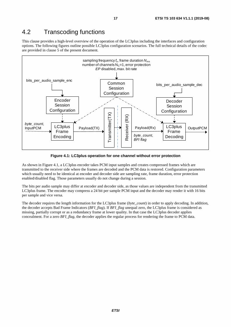
4.2 Transcoding functions This clause provides a high-level overview of the operation of the LC3plus including the interfaces and configuration options. The following figures outline possible LC3plus configuration scenarios. The full technical details of the codec are provided in clause 5 of the present document.
Figure 4.1: LC3plus operation for one channel without error protection
As shown in Figure 4.1, a LC3plus encoder takes PCM input samples and creates compressed frames which are transmitted to the receiver side where the frames are decoded and the PCM data is restored. Configuration parameters which usually need to be identical at encoder and decoder side are sampling rate, frame duration, error protection enabled/disabled flag. Those parameters usually do not change during a session.
The bits per audio sample may differ at encoder and decoder side, as those values are independent from the transmitted LC3plus frame. The encoder may compress a 24 bit per sample PCM input and the decoder may render it with 16 bits per sample and vice versa.
The decoder requires the length information for the LC3plus frame (byte_count) in order to apply decoding. In addition, the decoder accepts Bad Frame Indicators (BFI_flag). If BFI_flag unequal zero, the LC3plus frame is considered as missing, partially corrupt or as a redundancy frame at lower quality. In that case the LC3plus decoder applies concealment. For a zero BFI_flag, the decoder applies the regular process for rendering the frame to PCM data.
Tra
nsm
itter
(TX
)
Encoder Session
Configuration
byte_count,InputPCM LC3plus
Frame Encoding
Payload(TX)
bits_per_audio_sample_enc
Rec
eiv
er (
RX
)LC3plus Frame
Decoding
Payload(Rx)
Decoder Session
Configuration
bits_per_audio_sample_dec
OutputPCM
Common Session
Configuration
sampling frequency fs, frame duration Nms
number of channels NC=1, error protection EP disabled, max. bit rate
byte_count,BFI flag

ETSI
ETSI TS 103 634 V1.1.1 (2019-08)18
Figure 4.2: LC3plus operation for one channel including channel coder for error protection
Figure 4.2 outlines the LC3plus operation with enabled error protection where the channel coder is creating protected payloads.
The channel encoder is initialized with the number of gross bytes (channel coding bytes plus source coding bytes) and the EP_mode for selecting the strength of the error protection capability. The EP_mode can be changed on a frame by frame basis. Please note that for error protected payloads, the gross rate is usually kept constant for all EP modes. Increasing protection capability comes along with decreased bit rate for the codec. The channel coder requests a LC3plus frame with a certain codec rate (byte_count) depending on gross bytes and EP_mode.
The LC3plus channel decoder is able to detect the applied EP mode for a given gross rate and payload. It extracts the potentially corrected LC3plus frame and the related frame sizes (byte_count). The tool provides further information on the channel characteristic, e.g. the number of distorted bits. The channel decoder controls the BFI_flag signalling whether the payload is correct, partially correct or not reliable.
The channel coder also transports error protection mode requests (EPMR), a two-bit field indicating which EP mode should be used for encoding at the other side in bi-directional setups.
Tra
nsm
itter
(TX
)
Encoder Session
Configuration
InputPCM LC3plus Frame
Encoding
Payload(TX)
bits_per_audio_sample_enc
Rec
eive
r (R
X)
LCplusFrame
Decoding
Payload(Rx)
Decoder Session
Configuration
bits_per_audio_sample_dec
OutputPCM
Common Session
Configuration
sampling frequency fs, frame duration Nms,
number of channels NC=1,error protection EP enabled, max. bit rate
byte_count,BFI flag
LC3plus Channel Encoder
LCplusChannel Decoder
EP_mode, gross bytesbyte_count gross bytes
ETSI
ETSI TS 103 634 V1.1.1 (2019-08)19
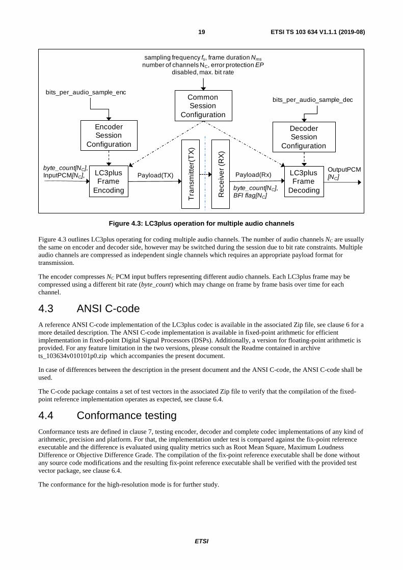
Figure 4.3: LC3plus operation for multiple audio channels
Figure 4.3 outlines LC3plus operating for coding multiple audio channels. The number of audio channels NC are usually the same on encoder and decoder side, however may be switched during the session due to bit rate constraints. Multiple audio channels are compressed as independent single channels which requires an appropriate payload format for transmission.
The encoder compresses NC PCM input buffers representing different audio channels. Each LC3plus frame may be compressed using a different bit rate (byte_count) which may change on frame by frame basis over time for each channel.
4.3 ANSI C-code A reference ANSI C-code implementation of the LC3plus codec is available in the associated Zip file, see clause 6 for a more detailed description. The ANSI C-code implementation is available in fixed-point arithmetic for efficient implementation in fixed-point Digital Signal Processors (DSPs). Additionally, a version for floating-point arithmetic is provided. For any feature limitation in the two versions, please consult the Readme contained in archive ts_103634v010101p0.zip which accompanies the present document.
In case of differences between the description in the present document and the ANSI C-code, the ANSI C-code shall be used.
The C-code package contains a set of test vectors in the associated Zip file to verify that the compilation of the fixed-point reference implementation operates as expected, see clause 6.4.
4.4 Conformance testing Conformance tests are defined in clause 7, testing encoder, decoder and complete codec implementations of any kind of arithmetic, precision and platform. For that, the implementation under test is compared against the fix-point reference executable and the difference is evaluated using quality metrics such as Root Mean Square, Maximum Loudness Difference or Objective Difference Grade. The compilation of the fix-point reference executable shall be done without any source code modifications and the resulting fix-point reference executable shall be verified with the provided test vector package, see clause 6.4.
The conformance for the high-resolution mode is for further study.
Tra
nsm
itter
(TX
)
Encoder Session
Configuration
byte_count[NC],InputPCM[NC], LC3plus
Frame Encoding
Payload(TX)
bits_per_audio_sample_enc
Rec
eiv
er (
RX
)
LC3plus Frame
Decoding
Payload(Rx)
Decoder Session
Configuration
bits_per_audio_sample_dec
OutputPCM[NC]
Common Session
Configuration
sampling frequency fs, frame duration Nms
number of channels NC, error protection EPdisabled, max. bit rate
byte_count[NC],BFI flag[NC]

ETSI
ETSI TS 103 634 V1.1.1 (2019-08)20
4.5 RTP payload format An RTP payload format for transporting LC3plus encoded audio in IP/UDP/RTP is defined in Annex B. The RTP payload format supports all possible combinations of frame durations, audio bandwidths and bitrates the LC3plus codec may generate.
The RTP payload format also defines configuration parameters that can be used to negotiate how the LC3plus codec can be used in a particular session, for example when the Session Description Protocol (SDP), IETF RFC 4566 [4], is used.
4.6 Performance characterization The LC3plus characterization is available in ETSI TR 103 633 [i.5].
NOTE: The TR is currently under study.
5 Codec algorithm description
5.1 General codec description This clause describes the technical specification of the Low Complexity Communication Codec plus (LC3plus). The main features of LC3plus coding one audio channel are:
Table 5.1: Feature summary
Feature Supported Range Frame duration 2,5 ms, 5 ms and 10 ms (2,72 ms, 5,44 ms, 10,88 ms @ 44,1 kHz) Look ahead delay 2,5 ms (2,72 ms @ 44,1 kHz)
Total algorithmic delay Frame duration + Look ahead delay = 5 ms, 7,5 ms, and 12,5 ms (for sampling rates other than 44,1 kHz)
Supported sampling rates 8, 16, 24, 32, 44,1 and 48 kHz Audio bandwidth Max. 20 kHz for 48 kHz
Supported Bit rate 20 to 400 bytes per frame and channel, e.g. 16 to 320 kbps per channel for 10 ms frame length and 48 kHz sampling rate
Supported bits per audio sample No restriction by the algorithm, however optimized for 16, 24, 32 bit depth input, see the limitation described in clause 5.2.3
The LC3plus furthermore features a high-resolution mode for sampling frequencies of 48 kHz and 96 kHz. The main features of this mode are:
Table 5.2: Feature Summary High-Resolution Mode
Feature Supported Range Frame duration 2,5 ms, 5 ms and 10 ms Look ahead delay 2,5 ms Total algorithmic delay Frame duration + Look ahead delay = 5 ms, 7,5 ms, and 12,5 ms Supported sampling rates 48 kHz and 96 kHz Audio bandwidth Always up to the Nyquist frequency
Supported Bit rate (per frame and channel)
Depends on sampling frequency and frame duration: • 156 to 625 bytes per frame at 48 kHz, 10 ms • 187 to 625 bytes per frame at 96 kHz, 10 ms • 93 to 375 bytes per frame at 48 kHz, 5 ms • 109 to 375 bytes per frame at 96 kHz, 5 ms • 54 to 210 bytes per frame at 48 kHz, 2,5 ms • 62 to 210 bytes per frame at 96 kHz, 2,5 ms
Supported bits per audio sample No restriction by the algorithm, however optimized for 24, 32 bit depth input, see the limitation described in clause 5.2.3
The high-resolution mode is not compatible with the other modes of LC3plus. The support and usage of the high-resolution mode shall be negotiated out of band. The high-resolution extension is described separately in clause 5.8 as a differential description to the clauses 5.2 to 5.7.
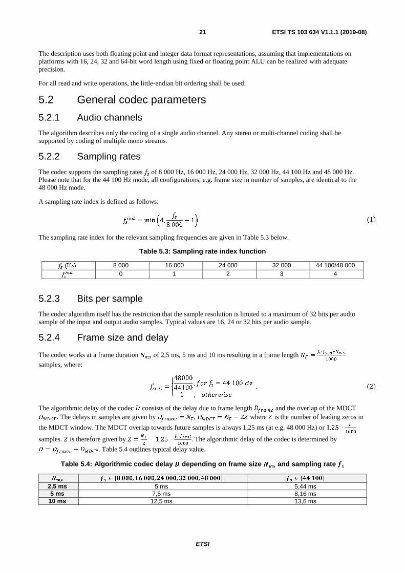
ETSI
ETSI TS 103 634 V1.1.1 (2019-08)21
The description uses both floating point and integer data format representations, assuming that implementations on platforms with 16, 24, 32 and 64-bit word length using fixed or floating point ALU can be realized with adequate precision.
For all read and write operations, the little-endian bit ordering shall be used.
5.2 General codec parameters
5.2.1 Audio channels
The algorithm describes only the coding of a single audio channel. Any stereo or multi-channel coding shall be supported by coding of multiple mono streams.
5.2.2 Sampling rates
The codec supports the sampling rates �� of 8 000 Hz, 16 000 Hz, 24 000 Hz, 32 000 Hz, 44 100 Hz and 48 000 Hz. Please note that for the 44 100 Hz mode, all configurations, e.g. frame size in number of samples, are identical to the 48 000 Hz mode.
A sampling rate index is defined as follows:
����� = min �4,��
8 000− 1� �1�
The sampling rate index for the relevant sampling frequencies are given in Table 5.3 below.
Table 5.3: Sampling rate index function
�� (Hz) 8 000 16 000 24 000 32 000 44 100/48 000
����� 0 1 2 3 4
5.2.3 Bits per sample
The codec algorithm itself has the restriction that the sample resolution is limited to a maximum of 32 bits per audio sample of the input and output audio samples. Typical values are 16, 24 or 32 bits per audio sample.
5.2.4 Frame size and delay
The codec works at a frame duration ��� of 2,5 ms, 5 ms and 10 ms resulting in a frame length �� =��∙�����∙���
����
samples, where:
����� = �48000
44100, ��� �� = 44 100 �
1 , �ℎ��� ��
. �2�
The algorithmic delay of the codec � consists of the delay due to frame length ������ and the overlap of the MDCT ����. The delays in samples are given by ������ = ��, ���� = �� − 2� where � is the number of leading zeros in
the MDCT window. The MDCT overlap towards future samples is always 1,25 ms (at e.g. 48 000 Hz) or 1,25 ∙��
����
samples. � is therefore given by � =��
�− 1,25 ∙
��∙�����
����. The algorithmic delay of the codec is determined by � = ������ + ����. Table 5.4 outlines typical delay value.
Table 5.4: Algorithmic codec delay ! depending on frame size "�� and sampling rate #� ��� ��
∈ [� ���,�� ���,� ���,� ���,� ���] ��
∈ [ ���] 2,5 ms 5 ms 5,44 ms 5 ms 7,5 ms 8,16 ms
10 ms 12,5 ms 13,6 ms
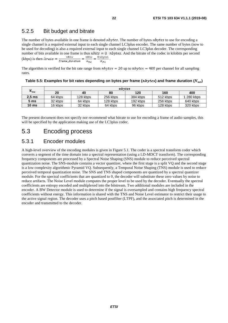
ETSI
ETSI TS 103 634 V1.1.1 (2019-08)22
5.2.5 Bit budget and bitrate
The number of bytes available in one frame is denoted ����. The number of bytes ���� to use for encoding a single channel is a required external input to each single channel LC3plus encoder. The same number of bytes (now to be used for decoding) is also a required external input to each single channel LC3plus decoder. The corresponding number of bits available in one frame is thus �� � = 8 ∙ ����. And the bitrate of the codec in kilobits per second
(kbps) is then ��� =�����
�����_��������=
�����
���
= ∙��!���
���
.
The algorithm is verified for the bit rate range from ���� = 20 up to ���� = 400 per channel for all sampling rates.
Table 5.5: Examples for bit rates depending on bytes per frame ($%&'()) and frame duration ("��)
��� �� ���
20 40 80 120 160 400 2,5 ms 64 kbps 128 kbps 256 kbps 384 kbps 512 kbps 1 280 kbps 5 ms 32 kbps 64 kbps 128 kbps 192 kbps 256 kbps 640 kbps
10 ms 16 kbps 32 kbps 64 kbps 96 kbps 128 kbps 320 kbps
The present document does not specify nor recommend what bitrate to use for encoding a frame of audio samples, this will be specified by the application making use of the LC3plus codec.
5.3 Encoding process
5.3.1 Encoder modules
A high-level overview of the encoding modules is given in Figure 5.1. The coder is a spectral transform coder which converts a segment of the time domain into a spectral representation (using a LD-MDCT transform). The corresponding frequency components are processed by a Spectral Noise Shaping (SNS) module to reduce perceived spectral quantization noise. The SNS-module contains a vector quantizer, where the first stage is a split VQ and the second stage is a low complexity algorithmic Pyramid VQ. Subsequently, a Temporal Noise Shaping (TNS) module is used to reduce perceived temporal quantization noise. The SNS and TNS shaped components are quantized by a spectral quantizer module. For the spectral coefficients that are quantized to 0, the decoder will substitute these zero values by noise to reduce artifacts. The Noise Level module computes the proper level to be used by the decoder. Eventually the spectral coefficients are entropy encoded and multiplexed into the bitstream. Two additional modules are included in the encoder. A BW Detector module is used to determine if the signal is oversampled and contains high frequency spectral coefficients without energy. This information is shared with the TNS and Noise Level estimator to restrict their usage to the active signal region. The decoder uses a pitch based postfilter (LTPF), and the associated pitch is determined in the encoder and transmitted to the decoder.
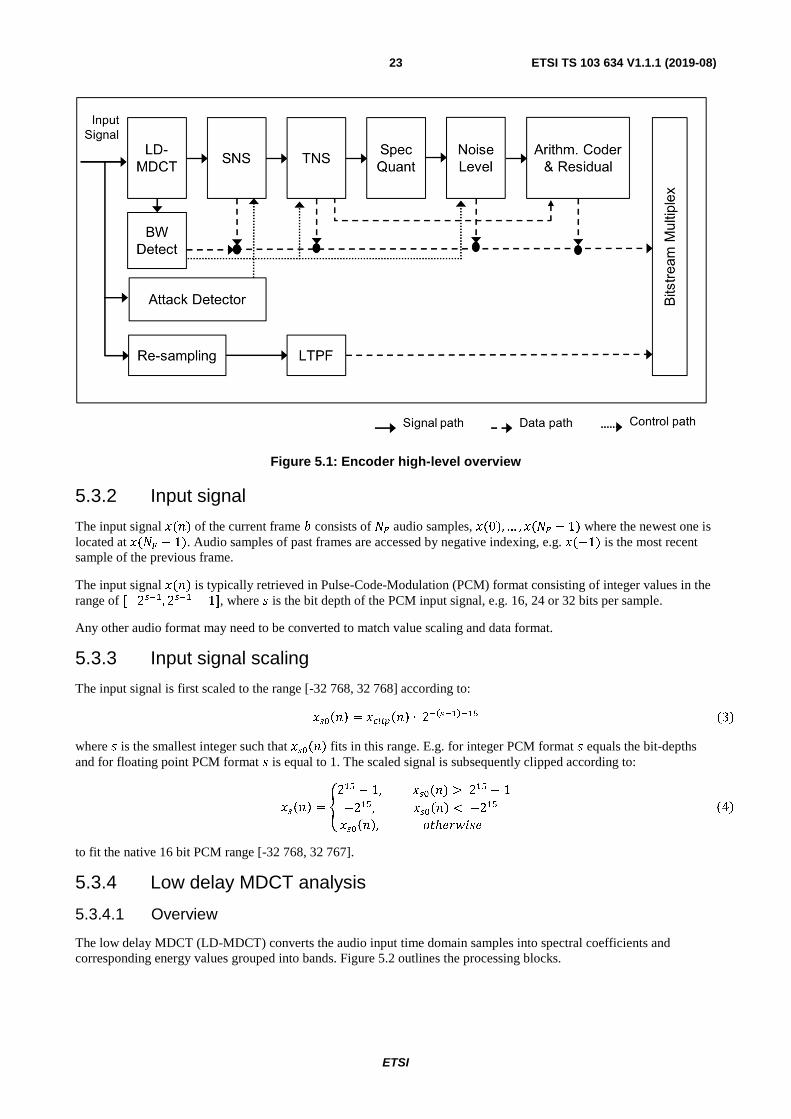
ETSI
ETSI TS 103 634 V1.1.1 (2019-08)23
Figure 5.1: Encoder high-level overview
5.3.2 Input signal
The input signal ���� of the current frame � consists of �� audio samples, ��0�, … , ���� 1� where the newest one is located at ���� 1�. Audio samples of past frames are accessed by negative indexing, e.g. ��1� is the most recent sample of the previous frame.
The input signal ���� is typically retrieved in Pulse-Code-Modulation (PCM) format consisting of integer values in the range of �2���, 2��� 1�, where � is the bit depth of the PCM input signal, e.g. 16, 24 or 32 bits per sample.
Any other audio format may need to be converted to match value scaling and data format.
5.3.3 Input signal scaling
The input signal is first scaled to the range [-32 768, 32 768] according to:
������ � ������� ∙ 2������� �3�
where � is the smallest integer such that ������ fits in this range. E.g. for integer PCM format � equals the bit-depths and for floating point PCM format � is equal to 1. The scaled signal is subsequently clipped according to:
����� � �2� 1, ������ � 2� 12� , ������ � 2� ������, ��ℎ������
�4�
to fit the native 16 bit PCM range [-32 768, 32 767].
5.3.4 Low delay MDCT analysis
5.3.4.1 Overview
The low delay MDCT (LD-MDCT) converts the audio input time domain samples into spectral coefficients and corresponding energy values grouped into bands. Figure 5.2 outlines the processing blocks.
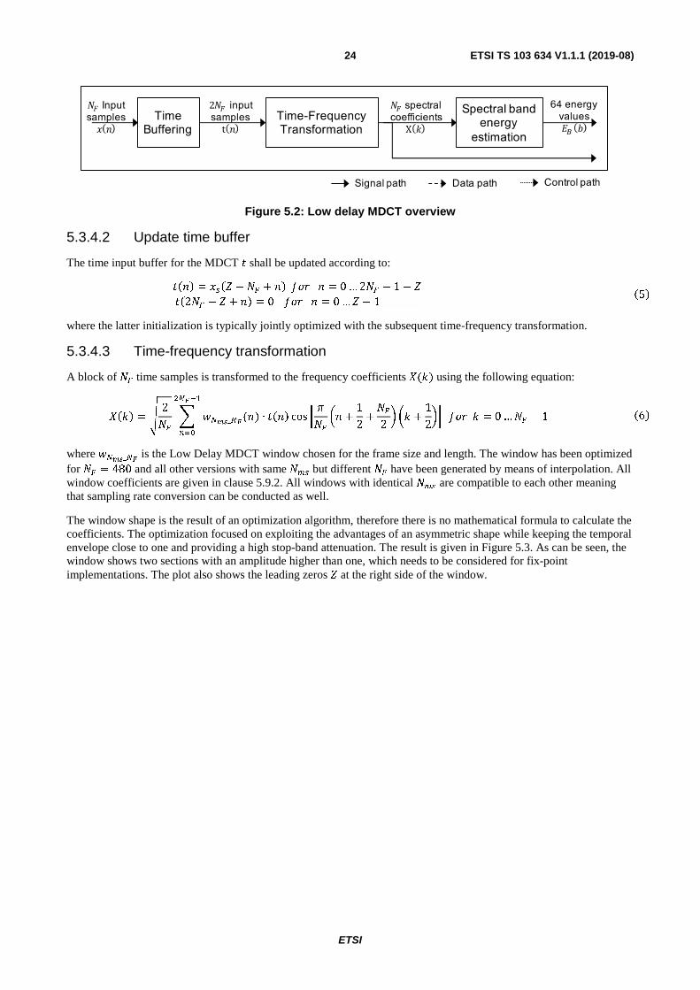
ETSI
ETSI TS 103 634 V1.1.1 (2019-08)24
Figure 5.2: Low delay MDCT overview
5.3.4.2 Update time buffer
The time input buffer for the MDCT � shall be updated according to:
���� = ���� − �� + �� � � = 0 … 2�� − 1 − ���2�� − � + �� = 0 � � = 0 …� − 1 �5�
where the latter initialization is typically jointly optimized with the subsequent time-frequency transformation.
5.3.4.3 Time-frequency transformation
A block of �� time samples is transformed to the frequency coefficients �(�) using the following equation:
���� = 2�� � ����_��(�) ∙ ���� cos � ��� �� +
1
2+��2� �� +
1
2�������
��
� � = 0 … �� − 1 �6� where ����_��
is the Low Delay MDCT window chosen for the frame size and length. The window has been optimized for �� = 480 and all other versions with same �� but different �� have been generated by means of interpolation. All window coefficients are given in clause 5.9.2. All windows with identical �� are compatible to each other meaning that sampling rate conversion can be conducted as well.
The window shape is the result of an optimization algorithm, therefore there is no mathematical formula to calculate the coefficients. The optimization focused on exploiting the advantages of an asymmetric shape while keeping the temporal envelope close to one and providing a high stop-band attenuation. The result is given in Figure 5.3. As can be seen, the window shows two sections with an amplitude higher than one, which needs to be considered for fix-point implementations. The plot also shows the leading zeros � at the right side of the window.
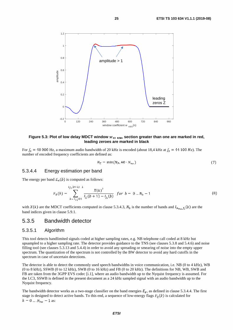
ETSI
ETSI TS 103 634 V1.1.1 (2019-08)25
Figure 5.3: Plot of low delay MDCT window ���_ ��, section greater than one are marked in red, leading zeroes are marked in black
For �� = 48 000 Hz, a maximum audio bandwidth of 20 kHz is encoded (about 18,4 kHz at �� = 44 100 ��). The number of encoded frequency coefficients are defined as:
�� = min(�� , 40 ∙ ��) �7� 5.3.4.4 Energy estimation per band
The energy per band ����� is computed as follows:
����� = � ���������� + 1� − ���������
�������
�� ������
� � = 0 … �� − 1 �8� with ���� are the MDCT coefficients computed in clause 5.3.4.3, �� is the number of bands and ����_��
��� are the band indices given in clause 5.9.1.
5.3.5 Bandwidth detector
5.3.5.1 Algorithm
This tool detects bandlimited signals coded at higher sampling rates, e.g. NB telephone call coded at 8 kHz but upsampled to a higher sampling rate. The detector provides guidance to the TNS (see clauses 5.3.8 and 5.4.6) and noise filling tool (see clauses 5.3.13 and 5.4.4) in order to avoid any spreading or smearing of noise into the empty upper spectrum. The quantization of the spectrum is not controlled by the BW detector to avoid any hard cutoffs in the spectrum in case of uncertain detections.
The detector is able to detect the commonly used speech bandwidths in voice communication, i.e. NB (0 to 4 kHz), WB (0 to 8 kHz), SSWB (0 to 12 kHz), SWB (0 to 16 kHz) and FB (0 to 20 kHz). The definitions for NB, WB, SWB and FB are taken from the 3GPP EVS codec [i.1], where an audio bandwidth up to the Nyquist frequency is assumed. For the LC3, SSWB is defined in the present document as a 24 kHz sampled signal with an audio bandwidth up to the Nyquist frequency.
The bandwidth detector works as a two-stage classifier on the band energies ��, as defined in clause 5.3.4.4. The first stage is designed to detect active bands. To this end, a sequence of low-energy flags ����� is calculated for � = 0 … ��� − 1 as:
0 120 240 360 480 600 720 840 960
window coefficient w 480(n)
-0.2
0
0.2
0.4
0.6
0.8
1
1.2
ampl
itude
leading zeros Z
amplitude > 1

ETSI
ETSI TS 103 634 V1.1.1 (2019-08)26
����� =
⎩⎨⎧
1 , � �������� ������� − ��� �������� + 1< �����
��� ������
�� ��� �������
0 , �ℎ �!"
�9� ���−1� is defined to be 0. The values of ��� �����(�) and ��� ����(�) are given in Table 5.6 and define frequency regions above the cut-off frequencies for the bandwidths in question. The quietness thresholds are given by �� = {20, 10, 10, 10}. The first stage classifier outputs a bandwidth index �� which is the largest index between 0 and ��� (with 0 and ��� included) such that ����� − 1� = 0.
The second stage determines the final bandwidth index ��. If �� = ���, then �� is set to ��. Otherwise, the second stage classifier aims at detecting an energy drop above the cut-off frequency of the candidate bandwidth ��. This is done by testing the condition:
max��� ������������������ � ��� �����������
#10$%� &��'� − (����)����� *+ > �!���� �10� where �! = {15, 23, 20, 20} and ( = {4, 4, 3, 1}. If this condition holds then �� is set to �� and otherwise it is set to ���. The parameter ,�� stores the final value ��.
The bandwidth information (NB, WB, SSWB, SWB, FB) is retrieved by mapping ,�� to the bandwidth column in Table 5.6. The bandwidth information is used to control the TNS and the Noise level estimation. The parameter ,�� is stored in the bit stream using the number of bits ��!�"�� as outlined in Table 5.6.
5.3.5.2 Parameters
Table 5.6 lists the used parameters to detect the active bandwidth for a given sampling rate �� and frame duration ��.
Table 5.6: Parameter table bandwidth detector
��� �� (Hz) ��� ��� ����� ��� ��� Bandwidth (���) ������ 2,5 ms 8 000 0 - - {NB} 0 2,5 ms 16 000 1 {24, 0, 0, 0} {34, 0, 0, 0} {NB, WB} 1 2,5 ms 24 000 2 {24, 35, 0, 0} {32, 39, 0, 0} {NB, WB, SSWB} 2 2,5 ms 32 000 3 {24, 33, 39, 0} {31, 38, 42, 0} {NB, WB, SSWB, SWB} 2 2,5 ms 44 100, 48 000 4 {22, 31, 37, 41} {29, 35, 40, 43} {NB, WB, SSWB, SWB, FB} 3 5 ms 8 000 0 - - {NB} 0 5 ms 16 000 1 {39, 0, 0, 0} {49, 0, 0, 0} {NB, WB} 1 5 ms 24 000 2 {35, 47, 0, 0} {44, 51, 0, 0} {NB, WB, SSWB} 2 5 ms 32 000 3 {34, 44, 50, 0} {42, 49, 53, 0} {NB, WB, SSWB, SWB} 3 5 ms 44 100, 48 000 4 {32, 42, 48, 52} {40, 46, 51, 54} {NB, WB, SSWB, SWB, FB} 4
10 ms 8 000 0 - - {NB} 0 10 ms 16 000 1 {53, 0, 0, 0} {63, 0, 0, 0} {NB, WB} 1 10 ms 24 000 2 {47, 59, 0, 0} {56, 63, 0, 0} {NB, WB, SSWB} 2 10 ms 32 000 3 {44, 54, 60, 0} {52, 59, 63, 0} {NB, WB, SSWB, SWB} 2 10 ms 44 100, 48 000 4 {41, 51, 57, 61} {49, 55, 60, 63} {NB, WB, SSWB, SWB, FB} 3
Note that when �� = 8 000 ��, the bandwidth detector is not needed and then the assignments ,�� = 0 and ��!�"�� = 0 are made, i.e. the parameter ,�� is not stored in the bit stream.
5.3.6 Time Domain Attack Detector
5.3.6.1 Overview
The time domain attack detector is active only for higher bit-rates, sampling rates �� ≥ 32 000 �� and a frame duration of 10 ms. Specifically, transient detection is carried out when �� = 320, 80 < ��-� " < 340 and �� = 10, or when �� = 480, 100 ≤ ��-� " < 340 and �� = 10.

ETSI
ETSI TS 103 634 V1.1.1 (2019-08)27
If active, the transient detector outputs a flag ����(�) for each frame �, which takes values 1, indicating that an attack was detected, or 0, indicating that no attack was detected in this frame. If not active, ������� is set to 0. In the following, the start-up frame index is denoted �.
5.3.6.2 Downsampling and Filtering of Input Signal
The first step is a downsampling of the input signal �����,� = 0 …�� − 1, which is performed as:
���������� = � �� � ��160
� + .����"
� �
�
� � = 0 … 159 �11� Next, the downsampled signal is high pass filtered according to:
�#������� = 0,375 ���������� − 0,5 ��������� − 1� + 0,125 ��������� − 2�, � � = 0 … 159. �12� As in the case of the input signal, samples at negative indices correspond to samples from previous frames, i.e. ��������−1� and ��������−2� hold the values ����������159� and ����������158�. The values ���������−1� and ���������−2� are defined to be zero.
5.3.6.3 Energy Calculation
The attack detector operates on block wise energies on 4 blocks of 40 samples.
���������� = � �#�����$��,� � = 0 … 3
$��%&
'�$�
, �13� which are compared to a delayed long term temporal envelope which is inductively defined by:
/��������� = max 00,25 /�������� − 1�, ��������� − 1�1, � � = 0 … 3, �14� where the values at index -1 correspond again to the values at index 3 in frame � − 1. The values /��������−1� and
���������−1� are defined to be zero.
5.3.6.4 Attack Detection
An attack is detected if:
���������� > 8,5 /������(�) �15�
holds for any � between 0 and 3. Furthermore, in this case the attack position ,���(�) is defined to be the largest n such that the inequality holds. Otherwise, ,���(�) is set to -1. The value ,���(� − 1) is defined to be -1.
The attack flag for frame � is computed as:
������� = 21
0
!� ,������ ≥ 0 ,����� − 1� ≥ 2, $" .�16�
5.3.7 Spectral Noise Shaping
5.3.7.1 Overview
Spectral Noise Shaping (SNS) applies a set of scale factors to the MDCT spectrum. These scale factors shape the quantization noise introduced in the frequency domain by the spectral quantization. The noise shaping is performed in such a way that the quantization noise is minimally perceived by the human ear, maximizing the perceptual quality of the decoded output.
The SNS encoder performs the following four steps. A set of 16 scale factors is first estimated as described in clause 5.3.7.2. These 16 scale factors are then quantized and encoded as described in clause 5.3.7.3. The quantized scale factors are then interpolated as described in clause 5.3.7.4. Finally, the MDCT spectrum is shaped using the 64 interpolated scale weights as described in clause 5.3.7.5. Figure 5.4 outlines the processing steps.
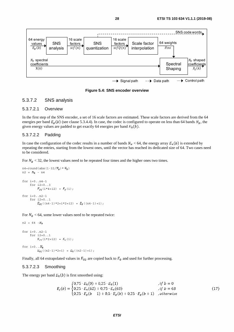
ETSI
ETSI TS 103 634 V1.1.1 (2019-08)28
Figure 5.4: SNS encoder overview
5.3.7.2 SNS analysis
5.3.7.2.1 Overview
In the first step of the SNS encoder, a set of 16 scale factors are estimated. These scale factors are derived from the 64 energies per band ����� (see clause 5.3.4.4). In case, the codec is configured to operate on less than 64 bands ��, the given energy values are padded to get exactly 64 energies per band �����. 5.3.7.2.2 Padding
In case the configuration of the codec results in a number of bands �� < 64, the energy array ����� is extended by repeating the entries, starting from the lowest ones, until the vector has reached its dedicated size of 64. Two cases need to be considered.
For �� < 32, the lowest values need to be repeated four times and the higher ones two times.
n4=round(abs(1-32/��)* ��) n2 = �� - n4
for i=0..n4-1 for i2=0..3 ���(i*4+i2) = ��(i); for i=0..n2-1 for i2=0..1 ���((n4-1)*2+i*2+i2) = ��((n4-1)+i);
For �� < 64, some lower values need to be repeated twice:
n2 = 64 -��
for i=0..n2-1 for i2=0..1 ���(i*2+i2) = ��(i); for i=0.. �� ���((n2-1)*2+i) = ��((n2-1)+i);
Finally, all 64 extrapolated values in ��� are copied back to �� and used for further processing.
5.3.7.2.3 Smoothing
The energy per band ����� is first smoothed using:
�(��� = 30,75 ∙ ���0� + 0,25 ∙ ���1� , !� � = 0
0,25 ∙ ���62� + 0,75 ∙ ���63� , !� � = 63
0,25 ∙ ���� − 1� + 0,5 ∙ ����� + 0,25 ∙ ���� + 1� , �ℎ �!" �17�

ETSI
ETSI TS 103 634 V1.1.1 (2019-08)29
5.3.7.2.4 Pre-emphasis
The smoothed energy per band �(��� is then pre-emphasized using:
�)��� = �(��� ∙ 10�∙*� ���∙"% � � = 0 … 63 �18�
with %�+'� given in Table 5.7.
Table 5.7: Pre-emphasis tilt factor table
�� (Hz) ��� 8 000 14
16 000 18 24 000 22 32 000 26
44 100, 48 000 30
5.3.7.2.5 Noise floor
A noise floor at -40 dB is added to �)��� using:
�)���� = max��)���,�!" �$� � � = 0 … 63 �19� with the noise floor being calculated by:
�!" �$ = max &∑ �)���"%��
64∙ 10
�$�, 2�%�* �20�
5.3.7.2.6 Logarithm
A transformation into the logarithm domain is then performed using:
����� =log�'�)����)
2 � � = 0 … 63 �21�
5.3.7.2.7 Band Energy Grouping
The vector ������, with �� ∈ [0, 63] is then grouped and decimated by a factor of 4 using:
������ =
⎩⎪⎪⎪⎨⎪⎪⎪⎧(0)��(0) + (�)
�
���
���4�� + � − 1� , � �� = 0
(�)
�
���
���4�� + � − 1� + �5���(63) , � �� = 15
(�)
�
���
���4�� + � − 1� , ��ℎ����� �22�
with �� ∈ [0, 15] and:
��� = � 1
12,
2
12,
3
12,
3
12,
2
12,
1
12� . �23�
5.3.7.2.8 Mean removal and scaling, attack handling
Mean removal and scaling is performed according to:
�� ����� = 0.85������� −∑ ���������
16� �� �� = 0. . .15. �24�
If the attack detection is not active or if it is active and ������ = 0, then the final scale factors are given by:
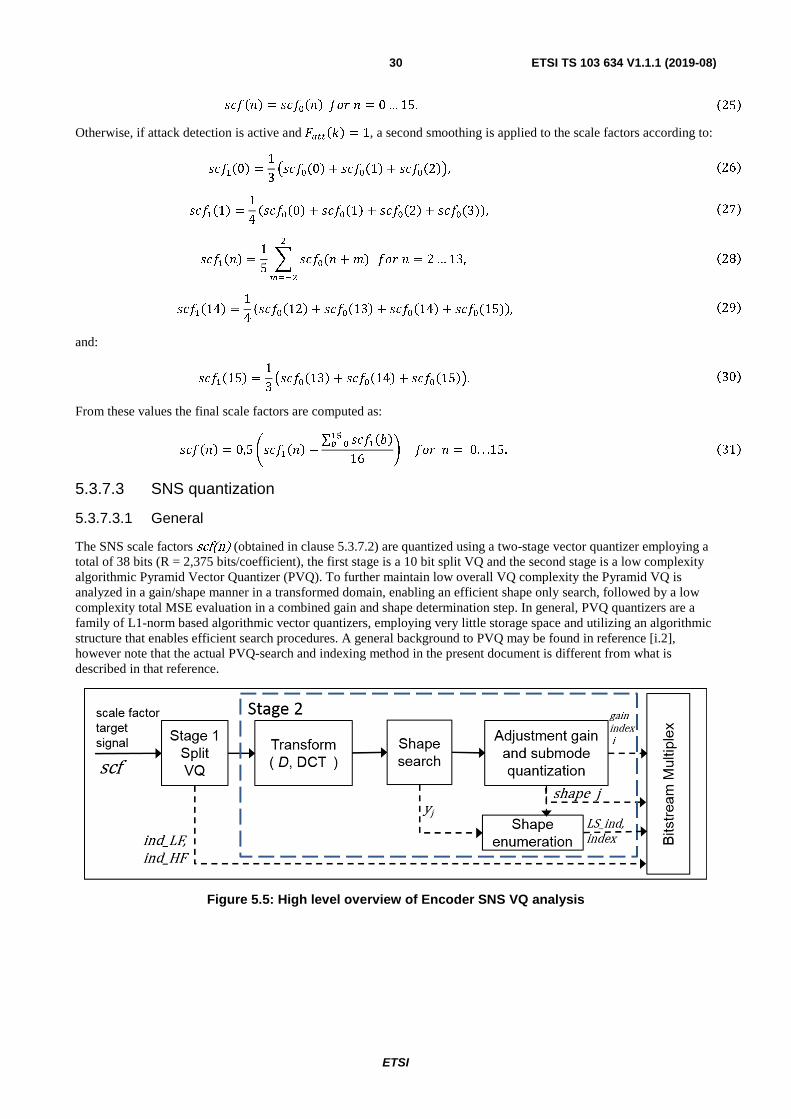
ETSI
ETSI TS 103 634 V1.1.1 (2019-08)30
������ � ������� � � � 0 … 15. �25�
Otherwise, if attack detection is active and ������� � 1, a second smoothing is applied to the scale factors according to:
�����0� � 13 ������0� � �����1� � �����2��, �26�
�����1� � 14 ������0� � �����1� � �����2� � �����3��, �27�
������� � 15 � ������ � ��
�
����
� � � 2 … 13, �28�
�����14� � 14 ������12� � �����13� � �����14� � �����15��, �29�
and:
�����15� � 13 ������13� � �����14� � �����15��. �30�
From these values the final scale factors are computed as:
������ � 0,5 �������� ∑ �����"��
��16 # � � � 0. . .15. �31�
5.3.7.3 SNS quantization
5.3.7.3.1 General
The SNS scale factors scf(n) (obtained in clause 5.3.7.2) are quantized using a two-stage vector quantizer employing a total of 38 bits (R = 2,375 bits/coefficient), the first stage is a 10 bit split VQ and the second stage is a low complexity algorithmic Pyramid Vector Quantizer (PVQ). To further maintain low overall VQ complexity the Pyramid VQ is analyzed in a gain/shape manner in a transformed domain, enabling an efficient shape only search, followed by a low complexity total MSE evaluation in a combined gain and shape determination step. In general, PVQ quantizers are a family of L1-norm based algorithmic vector quantizers, employing very little storage space and utilizing an algorithmic structure that enables efficient search procedures. A general background to PVQ may be found in reference [i.2], however note that the actual PVQ-search and indexing method in the present document is different from what is described in that reference.
Figure 5.5: High level overview of Encoder SNS VQ analysis

ETSI
ETSI TS 103 634 V1.1.1 (2019-08)31
5.3.7.3.2 Stage 1
The first stage is a split VQ employing two off-line trained stochastic codebooks LFCB and HFCB. Each codebook row has dimension 8 and the number of codebook columns is limited to 32, requiring 5 bits for each split for transmission. The MSE distortions for the two code books are defined as follows:
����_��� = ��� ��� − �� !����"�
���
�32�
����_#�� = ��� �� + 8� − #� !����"�
���
�33� The best index for the low-frequency split is found according to:
���_�� = argmin��[ � …. ��]
����_��� �34� The best index for the high-frequency split is found according to:
���_#� = argmin��[ � …. ��]
����_#�� �35� Codebooks LFCB and HFCB may be searched in any order.
The first stage vector is composed as:
��1��� = �� !���_��(�), �� � = $0 … 7%, �36� ��1�� + 8� = #� !��������, �� � = $0 … 7%. �37�
The first stage residual signal is calculated as:
�1��� = �� ��� − ��1���, �� � = $0 … 15%. �38� 5.3.7.3.3 Stage 2
5.3.7.3.3.1 General
On a high level the overall mean square error that is minimized by the second stage is:
������ℎ&'�_(,)&��_�, ���������,�*+,�������� =
-�1� − .���_�,����_� ∙ /0�,����� ,�����������,�*+,�������� ∙ 1�23��
�39� where Ggain_i,shape_j is a scalar value, D is a 16-by-16 rotation matrix (realizing an IDCT rotation) and xq,shape_j is a unit energy normalized vector of length 16. The �ℎ���_�, ����_�, �������, ���������� are vector quantization sub-indices that results in a total of 228 possible gain-shape combinations. The target of the second stage SNS VQ search is to find the set of indices that results in a minimum dMSE distortion value.
Depending on the selected shape index shape_j the number of leading sign indices LSindices are one {LS_indA } or two {LS_indA, LS_indB }, and similarly depending on the selected shape index shape_j the number of MPVQindices are one {idxA } or two {idxA, idxB }.
5.3.7.3.3.2 Transform
The second stage employs a 16-dimensional DCT-rotation using a 16x16 matrix D. The D-matrix has been determined off-line for efficient scale factor quantization, it has the property that DTD = I (the identity matrix). To reduce the encoder side search complexity the reverse(analysis) transform D (= DCT) may be used prior to the shape and gain determination, while on the decoder side only the forward(synthesis) transform DT (=IDCT) is required. The coefficients of the full D rotation matrix are listed in clause 5.9.3, here it should be noted that one may also use the equivalent conventional DCT (realized as the orthogonalized DCT-II) and the corresponding IDCT functions to realize these transformations.
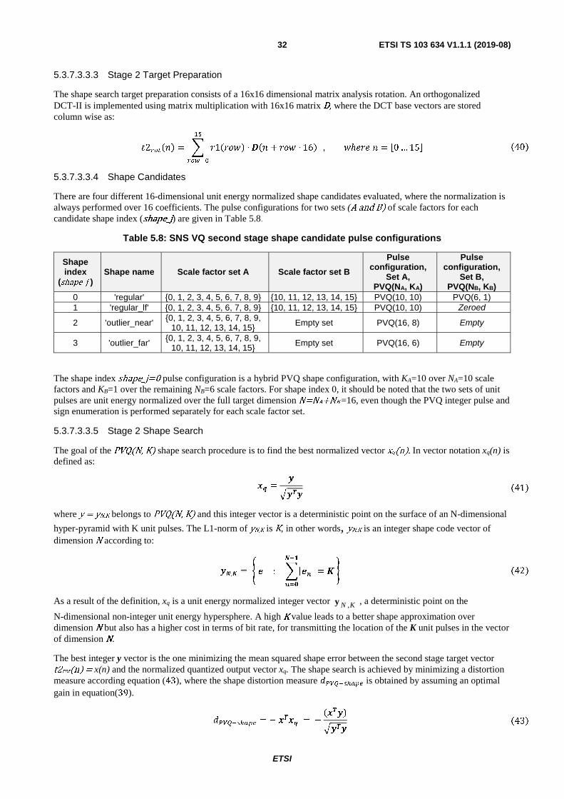
ETSI
ETSI TS 103 634 V1.1.1 (2019-08)32
5.3.7.3.3.3 Stage 2 Target Preparation
The shape search target preparation consists of a 16x16 dimensional matrix analysis rotation. An orthogonalized DCT-II is implemented using matrix multiplication with 16x16 matrix D, where the DCT base vectors are stored column wise as:
�2������ = � �1����� ∙ ��� + ��� ∙ 16���
�����
, �ℎ��� � = �0 … 15� �40�
5.3.7.3.3.4 Shape Candidates
There are four different 16-dimensional unit energy normalized shape candidates evaluated, where the normalization is always performed over 16 coefficients. The pulse configurations for two sets (A and B) of scale factors for each candidate shape index (shape_j) are given in Table 5.8.
Table 5.8: SNS VQ second stage shape candidate pulse configurations
Shape index
(shape_j ) Shape name Scale factor set A Scale factor set B
Pulse configuration,
Set A, PVQ(NA, KA)
Pulse configuration,
Set B, PVQ(NB, KB)
0 'regular' {0, 1, 2, 3, 4, 5, 6, 7, 8, 9} {10, 11, 12, 13, 14, 15} PVQ(10, 10) PVQ(6, 1) 1 'regular_lf' {0, 1, 2, 3, 4, 5, 6, 7, 8, 9} {10, 11, 12, 13, 14, 15} PVQ(10, 10) Zeroed
2 'outlier_near' {0, 1, 2, 3, 4, 5, 6, 7, 8, 9, 10, 11, 12, 13, 14, 15} Empty set PVQ(16, 8) Empty
3 'outlier_far' {0, 1, 2, 3, 4, 5, 6, 7, 8, 9, 10, 11, 12, 13, 14, 15} Empty set PVQ(16, 6) Empty
The shape index shape_j=0 pulse configuration is a hybrid PVQ shape configuration, with KA=10 over NA=10 scale factors and KB=1 over the remaining NB=6 scale factors. For shape index 0, it should be noted that the two sets of unit pulses are unit energy normalized over the full target dimension N=NA+NB =16, even though the PVQ integer pulse and sign enumeration is performed separately for each scale factor set.
5.3.7.3.3.5 Stage 2 Shape Search
The goal of the PVQ(N, K) shape search procedure is to find the best normalized vector xq(n). In vector notation xq(n) is defined as:
� =�
��� �41�
where y = yN.K belongs to PVQ(N, K) and this integer vector is a deterministic point on the surface of an N-dimensional
hyper-pyramid with K unit pulses. The L1-norm of yN,K is K, in other words, yN.K is an integer shape code vector of dimension N according to:
��,� = � � : �|� | = !
���
��
" �42�
As a result of the definition, xq is a unit energy normalized integer vector , a deterministic point on the
N-dimensional non-integer unit energy hypersphere. A high K value leads to a better shape approximation over dimension N but also has a higher cost in terms of bit rate, for transmitting the location of the K unit pulses in the vector of dimension N.
The best integer y vector is the one minimizing the mean squared shape error between the second stage target vector t2rot(n) = x(n) and the normalized quantized output vector xq. The shape search is achieved by minimizing a distortion measure according equation (43), where the shape distortion measure ���������� is obtained by assuming an optimal gain in equation(39).
���������� = − �� = −������� �43�
y KN ,
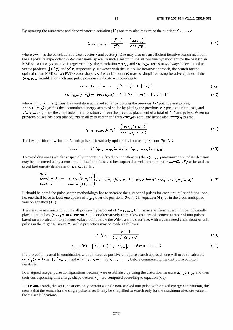
ETSI
ETSI TS 103 634 V1.1.1 (2019-08)33
By squaring the numerator and denominator in equation (43) one may also maximize the quotient QPVQ-shape:
���������� =������� =
#������$������%� �44�
where corrxy is the correlation between vector x and vector y. One may also use an efficient iterative search method in the all positive hyperoctant in N-dimensional space. In such a search in the all positive hyper-octant for the best (in an MSE sense) always positive integer vector �, the correlation ������ and �����%� terms may always be evaluated as vector products �|�|�� and ��, respectively. However with the unit pulse iterative approach, the search for the optimal (in an MSE sense) PVQ vector shape y(n) with L1-norm K, may be simplified using iterative updates of the QPVQ.-shape variables for each unit pulse position candidate �� according to:
�������&, ��� = �������& − 1� + 1 ∙ |'(��)| �45�
�����%��&, ��� = �����%��& − 1� + 2 ∙ 1� ∙ %�& − 1, ��� + 1� �46�
where corrxy(k-1) signifies the correlation achieved so far by placing the previous k-1 positive unit pulses, energyy(k-1) signifies the accumulated energy achieved so far by placing the previous k-1 positive unit pulses, and y(k-1, nc) signifies the amplitude of y at position nc from the previous placement of a total of k-1 unit pulses. When no previous pulses has been placed, y is an all zero vector and thus corrxy is zero, and hence also energyy is zero.
���������(�,�) =�������(�,�)� ����(�,�)
�47 The best position nbest for the kth unit pulse, is iteratively updated by increasing nc from 0 to N-1:
���� = � , �� �����������,� > �����������,���� �48 To avoid divisions (which is especially important in fixed point arithmetic) the QPVQ-shape maximization update decision may be performed using a cross-multiplication of a saved best squared correlation numerator bestCorrSq so far and the saved best energy denominator bestEn so far. ���� = ���������� = ��������,� ����� = ������,� � , �� ��������,� ∙ ����� > ��������� ∙ ����(�,�) �49 It should be noted the pulse search methodology has to increase the number of pulses for each unit pulse addition loop, i.e. one shall force at least one update of ���� over the positions 0 to N-1 in equation (48) or in the cross-multiplied version equation (49).
The iterative maximization in the all positive hyperoctant of QPVQ-shape(k, nc) may start from a zero number of initially placed unit pulses (ystart(n) = 0, for n=0...15) or alternatively from a low cost pre-placement number of unit pulses based on an projection to a integer valued point below the K'th-pyramid's surface, with a guaranteed undershoot of unit pulses in the target L1 norm K. Such a projection may be made as follows:
������ = � − 1∑ |�2���(�)|����
���
�50 �������� = �|�2����� | ∙ �������, ��� � = 0 … 15 �51
If a projection is used in combination with an iterative positive unit pulse search approach one will need to calculate �������� − 1 as �|�|� ����� and ������ − 1 as ������ ����� before commencing the unit pulse addition iterations.
Four signed integer pulse configurations vectors yj are established by using the distortion measure !�������� and then their corresponding unit energy shape vectors "�,� are computed according to equation (41).
In the j=0 search, the set B positions only contain a single non-stacked unit pulse with a fixed energy contribution, this means that the search for the single pulse in set B may be simplified to search only for the maximum absolute value in the six set B locations.

ETSI
ETSI TS 103 634 V1.1.1 (2019-08)34
For the j=0,1 normalization, each total pulse configuration yj always spans 16 coefficients. Hence, the energy normalization is always performed over dimension 16, even though two shorter position sets are used for enumeration of the y0 integer vector and one position set (set A) of dimension 10 for the y1 integer vector.
An efficient overall unit pulse search (for all four shape candidates) may be achieved by searching the shapes in the order from shape j=3 to shape j=0, by making a first projection to a point on or below the pyramid K=6, updating the correlation and energy terms, and then sequentially adding unit pulses and saving intermediate shape results until K is correct for each of the four shape candidates with a higher number of unit pulses K. Note that as the regular set A shapes j=0,1 spans over different allowed scale factor dimensions/regions than the two outlier shapes (j=2,3 ), one will need to handle the search start pulse configuration for the two regular shapes by removing any unit pulses which are not possible to index in the regular shape set A(j=0,1). As the described iterative pulse search is performed in the all positive hyperoctant, a final step of setting the signs of the non-zero entries in yj (n) based on the corresponding sign in target vector x(n)= t2rot(n) is performed.
A step-by-step example of a search procedure is shown in Table 5.9 and example of resulting vectors are shown in Table 5.10.
Table 5.9: Informational example of a PVQ search strategy for the described PVQ based shapes
Search step
Related shape index
(j )
Description of search step Resulting vector
1 3 Project to or below pyramid N=16, K=6, (and update energy energyy and correlation corrxy terms to reflect the pulses present in y3, start )
y3,start
2 3 Add unit pulses until K=6 is reached over N=16 samples, save y3 y3 =y2,start
3 2 Add unit pulses until K=8 is reached over N=16 samples, save y2
y2 =y1,pre-start
4 1 Remove any unit pulses in y1,pre-start that are not part of set A to yield y1, start y1, start
5 1 Update energy energyy and correlation corrxy terms to reflect the pulses present in y1, start
y1, start (unchanged)
6 1 Add unit pulses until K=10 is reached over N=10 samples (in set A), save y1 y1=y0,start
7 0 Add unit pulses to y0,start until K=1 is reached over N=6 samples (in set B), save y0
y0
8 3, 2, 1, 0 Add signs to non-zero positions of each yj vector from the target vector x, save y3, y2, y1, y0 as shape vector candidates (and for subsequent indexing of one of them)
y3, y2, y1, y0
9 3, 2, 1, 0 Unit energy normalize each yj vector to candidate vector xq.j xq,3, xq,2, xq,1, xq,0
Table 5.10: Informational example of potentially available integer vectors yj and their corresponding unit energy normalized vectors xq,j , after completing the PVQ search
Shape index
(j) Example Integer vector yj
Corresponding unit energy normalized vector xq,j (NB! Shown in very low precision here)
0 y0 = [-10, 0, 0, 0, 0, 0, 0, 0, 0, 0, 0, 0, 0, 0, 0, 1] xq,0 = [-0,995, 0, 0, 0, 0, 0, 0, 0, 0, 0, 0, 0, 0, 0, 0, 0,100] 1 y1 = [0, 0, 0, 0, 0, 0, 0, 0, 0, 10, 0, 0, 0, 0, 0, 0] xq,1 = [0, 0, 0, 0, 0, 0, 0, 0, 0, 1,0, 0, 0, 0, 0, 0, 0] 2 y2 = [0, 0, 0, 0, 0, 0, 0, 0, 0, 1, 0, 0, 0, 0, 0, -7] xq,2 = [0, 0, 0, 0, 0, 0, 0, 0, 0, 0,141, 0, 0, 0, 0, 0, -0,990]
3 y3 = [0, 0, 0, 0, 0, 0, 0, 0, 0, 0, -1, 1, -1, 1,
-1, 1] xq,3 = [0, 0, 0, 0, 0, 0, 0, 0, 0, 0, -0,408, 0,408, -0,408, 0,408,
-0,408, 0,408]
5.3.7.3.3.6 Adjustment Gain Candidates
There are four different adjustment gain candidate sets, one set corresponding to each overall shape candidate j. The adjustment gain configuration for each of the shapes are given in Table 5.11.
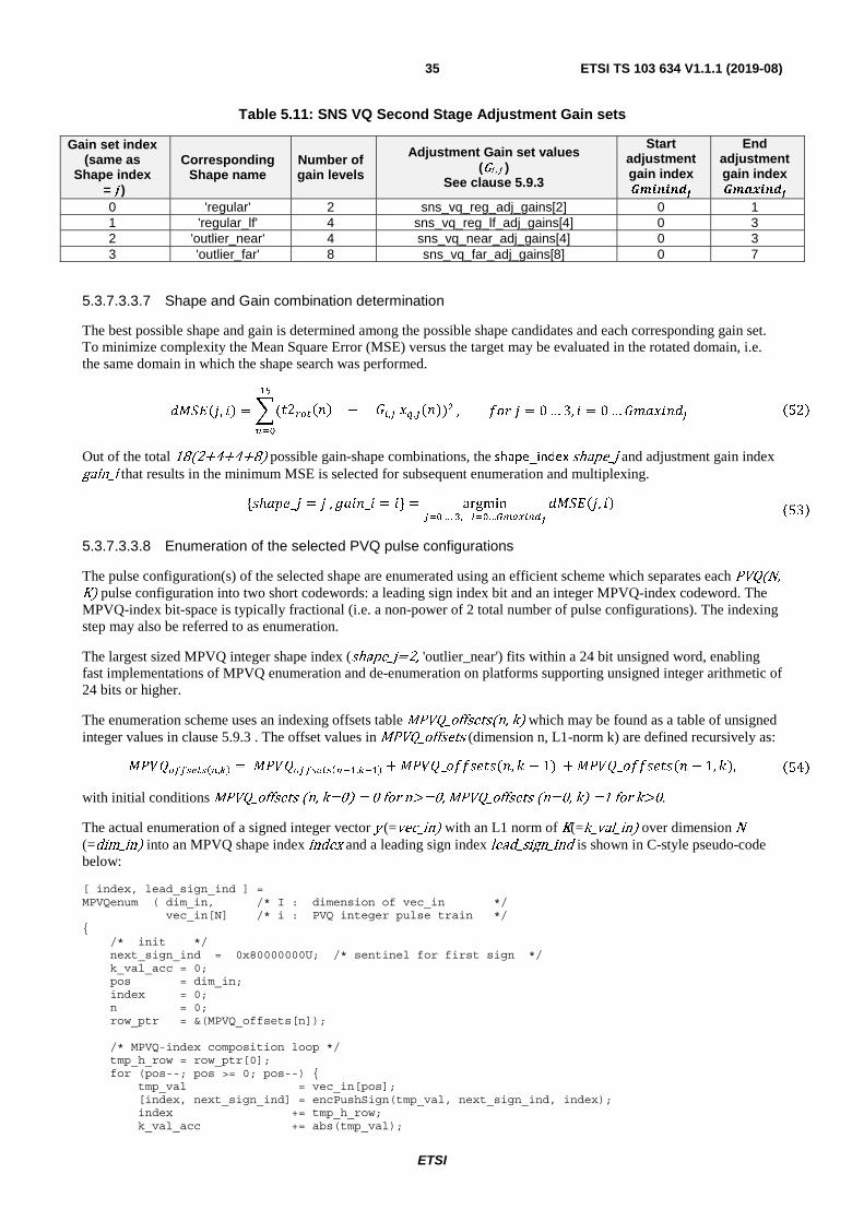
ETSI
ETSI TS 103 634 V1.1.1 (2019-08)35
Table 5.11: SNS VQ Second Stage Adjustment Gain sets
Gain set index (same as
Shape index = j )
Corresponding Shape name
Number of gain levels
Adjustment Gain set values (Gi , j )
See clause 5.9.3
Start adjustment gain index ��������
End adjustment gain index ��������
0 'regular' 2 sns_vq_reg_adj_gains[2] 0 1 1 'regular_lf' 4 sns_vq_reg_lf_adj_gains[4] 0 3 2 'outlier_near' 4 sns_vq_near_adj_gains[4] 0 3 3 'outlier_far' 8 sns_vq_far_adj_gains[8] 0 7
5.3.7.3.3.7 Shape and Gain combination determination
The best possible shape and gain is determined among the possible shape candidates and each corresponding gain set. To minimize complexity the Mean Square Error (MSE) versus the target may be evaluated in the rotated domain, i.e. the same domain in which the shape search was performed.
������, �� = �2������ − ��,� �,�(�)���
��
, ��� � = 0 … 3, � = 0 …��� ���� �52�
Out of the total 18(2+4+4+8) possible gain-shape combinations, the shape_index shape_j and adjustment gain index gain_i that results in the minimum MSE is selected for subsequent enumeration and multiplexing.
{�ℎ���_� = � ,����_� = �} = argmin��� … �, ���…������
�� �, �� 53�
5.3.7.3.3.8 Enumeration of the selected PVQ pulse configurations
The pulse configuration(s) of the selected shape are enumerated using an efficient scheme which separates each PVQ(N,
K) pulse configuration into two short codewords: a leading sign index bit and an integer MPVQ-index codeword. The MPVQ-index bit-space is typically fractional (i.e. a non-power of 2 total number of pulse configurations). The indexing step may also be referred to as enumeration.
The largest sized MPVQ integer shape index (shape_j=2, 'outlier_near') fits within a 24 bit unsigned word, enabling fast implementations of MPVQ enumeration and de-enumeration on platforms supporting unsigned integer arithmetic of 24 bits or higher.
The enumeration scheme uses an indexing offsets table MPVQ_offsets(n, k) which may be found as a table of unsigned integer values in clause 5.9.3 . The offset values in MPVQ_offsets (dimension n, L1-norm k) are defined recursively as:
���� �����,�� = ���� �������,���� + ���_�������(�, � − 1) + ���_�������(� − 1, �), 54�
with initial conditions MPVQ_offsets (n, k=0) = 0 for n>=0, MPVQ_offsets (n=0, k) =1 for k>0.
The actual enumeration of a signed integer vector y
(=vec_in) with an L1 norm of K(=k_val_in) over dimension N
(=dim_in) into an MPVQ shape index index and a leading sign index lead_sign_ind is shown in C-style pseudo-code below:
[ index, lead_sign_ind ] = MPVQenum ( dim_in, /* I : dimension of vec_in */ vec_in[N] /* i : PVQ integer pulse train */ { /* init */ next_sign_ind = 0x80000000U; /* sentinel for first sign */ k_val_acc = 0; pos = dim_in; index = 0; n = 0; row_ptr = &(MPVQ_offsets[n]); /* MPVQ-index composition loop */ tmp_h_row = row_ptr[0]; for (pos--; pos >= 0; pos--) { tmp_val = vec_in[pos]; [index, next_sign_ind] = encPushSign(tmp_val, next_sign_ind, index); index += tmp_h_row; k_val_acc += abs(tmp_val);
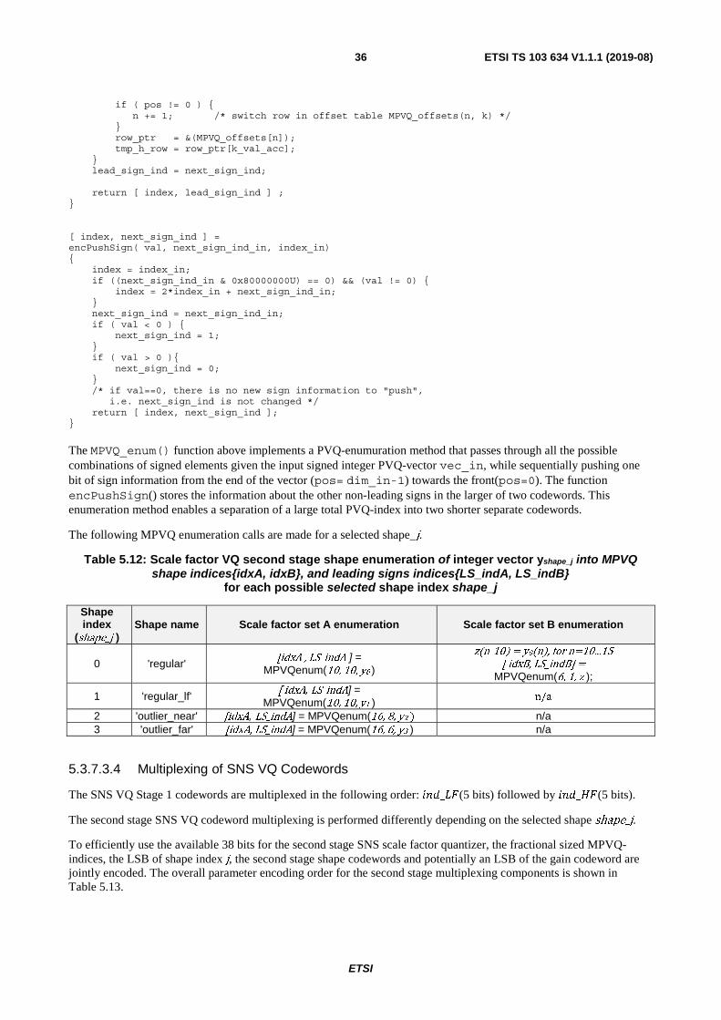
ETSI
ETSI TS 103 634 V1.1.1 (2019-08)36
if ( pos != 0 ) { n += 1; /* switch row in offset table MPVQ_offsets(n, k) */ } row_ptr = &(MPVQ_offsets[n]); tmp_h_row = row_ptr[k_val_acc]; } lead_sign_ind = next_sign_ind; return [ index, lead_sign_ind ] ; } [ index, next_sign_ind ] = encPushSign( val, next_sign_ind_in, index_in) { index = index_in; if ((next_sign_ind_in & 0x80000000U) == 0) && (val != 0) { index = 2*index_in + next_sign_ind_in; } next_sign_ind = next_sign_ind_in; if ( val < 0 ) { next_sign_ind = 1; } if ( val > 0 ){ next_sign_ind = 0; } /* if val==0, there is no new sign information to "push", i.e. next_sign_ind is not changed */ return [ index, next_sign_ind ]; }
The MPVQ_enum() function above implements a PVQ-enumuration method that passes through all the possible combinations of signed elements given the input signed integer PVQ-vector vec_in, while sequentially pushing one bit of sign information from the end of the vector (pos= dim_in-1) towards the front(pos=0). The function encPushSign() stores the information about the other non-leading signs in the larger of two codewords. This enumeration method enables a separation of a large total PVQ-index into two shorter separate codewords.
The following MPVQ enumeration calls are made for a selected shape_j.
Table 5.12: Scale factor VQ second stage shape enumeration of integer vector yshape_j into MPVQ shape indices{idxA, idxB}, and leading signs indices{LS_indA, LS_indB}
for each possible selected shape index shape_j
Shape index
(shape_j ) Shape name Scale factor set A enumeration Scale factor set B enumeration
0 'regular' [idxA , LS_indA ] =
MPVQenum(10, 10, y0 )
z(n-10) = y0(n), for n=10...15
[ idxB, LS_indB] = MPVQenum(6, 1, z );
1 'regular_lf' [ idxA, LS_indA] =
MPVQenum(10, 10, y1 ) n/a
2 'outlier_near' [idxA, LS_indA] = MPVQenum(16, 8, y2 ) n/a 3 'outlier_far' [idxA, LS_indA] = MPVQenum(16, 6, y3 ) n/a
5.3.7.3.4 Multiplexing of SNS VQ Codewords
The SNS VQ Stage 1 codewords are multiplexed in the following order: ���_��(5 bits) followed by ���_��(5 bits).
The second stage SNS VQ codeword multiplexing is performed differently depending on the selected shape shape_j.
To efficiently use the available 38 bits for the second stage SNS scale factor quantizer, the fractional sized MPVQ-indices, the LSB of shape index j, the second stage shape codewords and potentially an LSB of the gain codeword are jointly encoded. The overall parameter encoding order for the second stage multiplexing components is shown in Table 5.13.
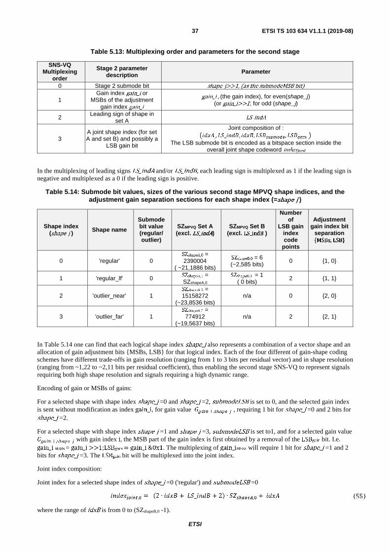
ETSI
ETSI TS 103 634 V1.1.1 (2019-08)37
Table 5.13: Multiplexing order and parameters for the second stage
SNS-VQ Multiplexing
order
Stage 2 parameter description Parameter
0 Stage 2 submode bit shape_j>>1, (as the submodeMSB bit)
1 Gain index gain_i or
MSBs of the adjustment gain index gain_i
gain_i , (the gain index), for even(shape_j) (or gain_i>>1; for odd (shape_j)
2 Leading sign of shape in
set A LS_indA
3 A joint shape index (for set A and set B) and possibly a
LSB gain bit
Joint composition of : �����
,, ��_���, ���, ��������� , ����
The LSB submode bit is encoded as a bitspace section inside the overall joint shape codeword indexjoint
In the multiplexing of leading signs LS_indA and/or LS_indB, each leading sign is multiplexed as 1 if the leading sign is negative and multiplexed as a 0 if the leading sign is positive.
Table 5.14: Submode bit values, sizes of the various second stage MPVQ shape indices, and the adjustment gain separation sections for each shape index (=shape_j )
Shape index (shape_j ) Shape name
Submode bit value (regular/ outlier)
SZMPVQ Set A (excl. LS_indA)
SZMPVQ Set B (excl. LS_indB )
Number of
LSB gain index code
points
Adjustment gain index bit
separation {MSBs, LSB}
0 'regular' 0 SZshapeA,0 = 2390004
( ~21,1886 bits)
SZshapeB,0 = 6 (~2,585 bits)
0 {1, 0}
1 'regular_lf' 0 SZshapeA,1 = SZshapeA,0
SZshapeB,1 = 1 ( 0 bits)
2 {1, 1}
2 'outlier_near' 1 SZshapeA,2 = 15158272
(~23,8536 bits) n/a 0 {2, 0}
3 'outlier_far' 1 SZshapeA,3 =
774912 (~19,5637 bits)
n/a 2 {2, 1}
In Table 5.14 one can find that each logical shape index shape_j also represents a combination of a vector shape and an allocation of gain adjustment bits {MSBs, LSB} for that logical index. Each of the four different of gain-shape coding schemes have different trade-offs in gain resolution (ranging from 1 to 3 bits per residual vector) and in shape resolution (ranging from ~1,22 to ~2,11 bits per residual coefficient), thus enabling the second stage SNS-VQ to represent signals requiring both high shape resolution and signals requiring a high dynamic range.
Encoding of gain or MSBs of gains:
For a selected shape with shape index shape_j =0 and shape_j =2, submodeLSB is set to 0, and the selected gain index is sent without modification as index gain_i, for gain value �����_� ,�����_ , requiring 1 bit for shape_j =0 and 2 bits for shape_j =2.
For a selected shape with shape index shape_j =1 and shape_j =3, submodeLSB is set to1, and for a selected gain value �����_� ,�����_ with gain index i, the MSB part of the gain index is first obtained by a removal of the LSBgain bit. I.e. gain_i MSBs = gain_i >>1;LSBgain = gain_i &0x1. The multiplexing of gain_iMSBs will require 1 bit for shape_j =1 and 2 bits for shape_j =3. The LSBgain bit will be multiplexed into the joint index.
Joint index composition:
Joint index for a selected shape index of shape_j =0 ('regular') and submodeLSB =0
��������,� = �2 ∙ ���� + _���� + 2� ∙ ������ ,� + ��� �55�
where the range of idxB is from 0 to (SZshapeB,0 -1).
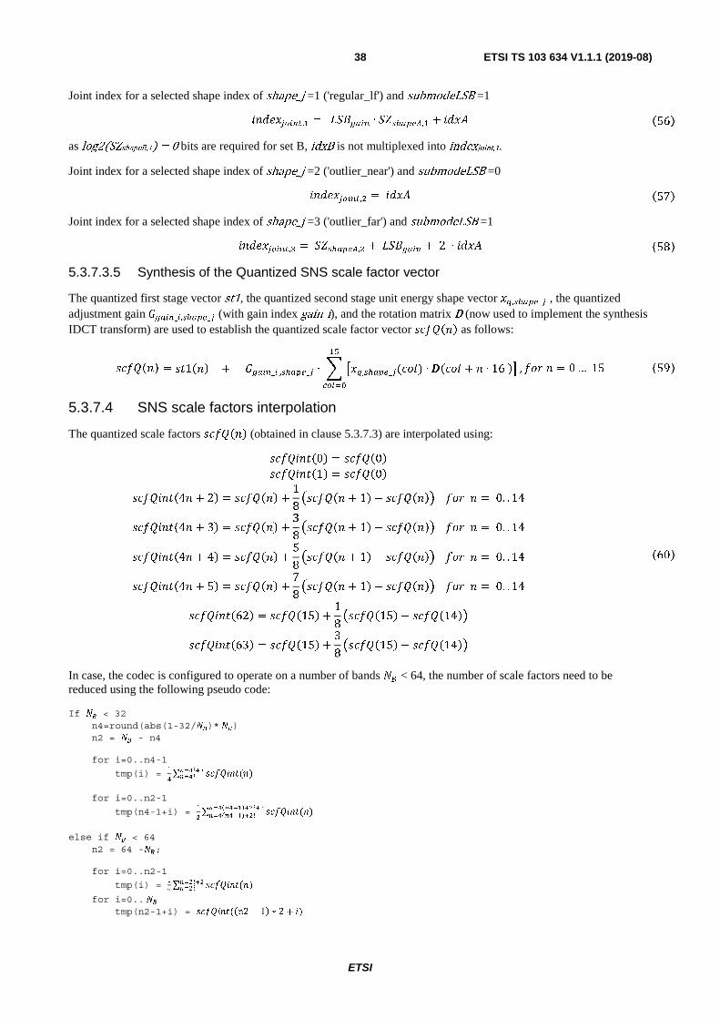
ETSI
ETSI TS 103 634 V1.1.1 (2019-08)38
Joint index for a selected shape index of shape_j =1 ('regular_lf') and submodeLSB =1
��������,� = ����� ∙ ������ ,� + ��� �56�
as log2(SZshapeB,1) = 0 bits are required for set B, idxB is not multiplexed into indexjoint,1.
Joint index for a selected shape index of shape_j =2 ('outlier_near') and submodeLSB =0
����������,� = ���� �57� Joint index for a selected shape index of shape_j =3 ('outlier_far') and submodeLSB =1
����������,� = ��� ,� + ����� + 2 ∙ ���� �58� 5.3.7.3.5 Synthesis of the Quantized SNS scale factor vector
The quantized first stage vector st1, the quantized second stage unit energy shape vector ��,���_� , the quantized adjustment gain ���_�,���_� (with gain index gain_i), and the rotation matrix D (now used to implement the synthesis IDCT transform) are used to establish the quantized scale factor vector ������� as follows:
������� = ��1��� + ���_� ,���_� ∙ � ���,���_�(���) ∙ ����� + � ∙ 16 �� ��
�����
, ��� � = 0 … 15 �59�
5.3.7.4 SNS scale factors interpolation
The quantized scale factors ������� (obtained in clause 5.3.7.3) are interpolated using:
��������0� = �����0���������1� = �����0�
��������4� + 2� = ������� +1
8������� + 1� − �������� ��� � = 0. . 14
��������4� + 3� = ������� +3
8������� + 1� − �������� ��� � = 0. . 14
��������4� + 4� = ������� +5
8������� + 1� − �������� ��� � = 0. . 14
��������4� + 5� = ������� +7
8������� + 1� − �������� ��� � = 0. . 14
��������62� = �����15� +1
8������15� − �����14��
��������63� = �����15� +3
8������15� − �����14��
�60�
In case, the codec is configured to operate on a number of bands �� < 64, the number of scale factors need to be reduced using the following pseudo code:
If �� < 32 n4=round(abs(1-32/��)* ��) n2 = �� - n4 for i=0..n4-1
tmp(i) = �
�∑ ������(�)����������
for i=0..n2-1
tmp(n4-1+i) = �
∑ ������(�)�����������
����������
else if �� < 64 n2 = 64 -��;
for i=0..n2-1
tmp(i) = �
∑ ������(�)�������
for i=0.. �� tmp(n2-1+i) = ������(n2 − 1� ∗ 2 + �)
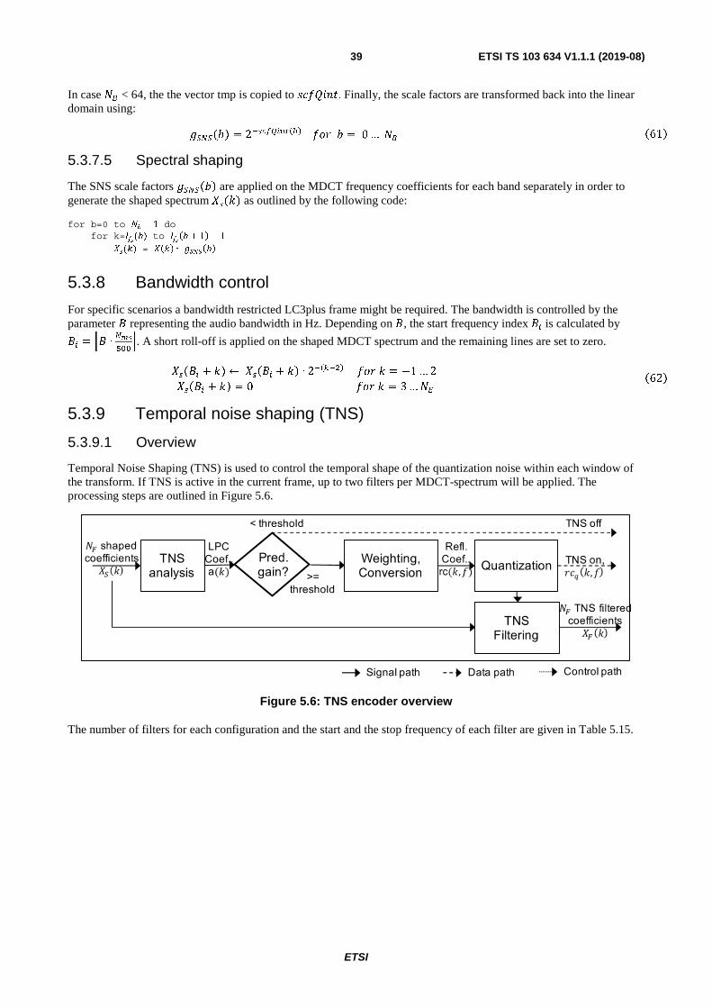
ETSI
ETSI TS 103 634 V1.1.1 (2019-08)39
In case �� < 64, the the vector tmp is copied to �������. Finally, the scale factors are transformed back into the linear domain using:
������� = 2����������� ��� � = 0 … �� �61� 5.3.7.5 Spectral shaping
The SNS scale factors ������� are applied on the MDCT frequency coefficients for each band separately in order to generate the shaped spectrum ��( ) as outlined by the following code:
for b=0 to � − 1 do for k=���( ) to ��� + 1� − 1
��(�) = ��� ∙ ���� �
5.3.8 Bandwidth control
For specific scenarios a bandwidth restricted LC3plus frame might be required. The bandwidth is controlled by the parameter � representing the audio bandwidth in Hz. Depending on �, the start frequency index �� is calculated by
�� = !� ∙���
���". A short roll-off is applied on the shaped MDCT spectrum and the remaining lines are set to zero.
����� + � ← ����� + � ∙ 2��� �� ��� = −1 … 2
����� + � = 0 ��� = 3 …�! �62�
5.3.9 Temporal noise shaping (TNS)
5.3.9.1 Overview
Temporal Noise Shaping (TNS) is used to control the temporal shape of the quantization noise within each window of the transform. If TNS is active in the current frame, up to two filters per MDCT-spectrum will be applied. The processing steps are outlined in Figure 5.6.
Figure 5.6: TNS encoder overview
The number of filters for each configuration and the start and the stop frequency of each filter are given in Table 5.15.
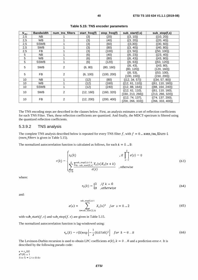
ETSI
ETSI TS 103 634 V1.1.1 (2019-08)40
Table 5.15: TNS encoder parameters
���
Bandwidth num_tns_filters start_freq(f) stop_freq(f) sub_start(f,s) sub_stop(f,s) 2,5 NB 1 {3} {20} {{3, 10}} {{10, 20}} 2,5 WB 1 {3} {40} {{3, 20}} {{20, 40}} 2,5 SSWB 1 {3} {60} {{3,30}} {{30, 60}} 2,5 SWB 1 {3} {80} {{3, 40}} {{40, 80}} 2,5 FB 1 {3} {100} {{3, 50}} {{50, 100}} 5 NB 1 {6} {40} {{6, 23}} {{23, 40}} 5 WB 1 {6} {80} {{6, 43}} {{43, 80}} 5 SSWB 1 {6} {120} {{6, 63}} {{63, 120}}
5 SWB 2 {6, 80} {80, 160} {{6, 43}, {80, 120}}
{{43, 80}, {120, 160}}
5 FB 2 {6, 100} {100, 200} {{6, 53}, {100, 150}}
{{53, 100}, {150, 200}}
10 NB 1 {12} {80} {{12, 34, 57}} {{34, 57, 80}} 10 WB 1 {12} {160} {{12, 61, 110}} {{61, 110, 160}} 10 SSWB 1 {12} {240} {{12, 88, 164}} {{88, 164, 240}}
10 SWB 2 {12, 160} {160, 320} {{12, 61, 110}, {160, 213, 266}}
{{61, 110, 160}, {213, 266, 320}}
10 FB 2 {12, 200} {200, 400} {{12, 74, 137}, {200, 266, 333}}
{{74, 137, 200}, {266, 333, 400}}
The TNS encoding steps are described in the clauses below. First, an analysis estimates a set of reflection coefficients for each TNS Filter. Then, these reflection coefficients are quantized. And finally, the MDCT-spectrum is filtered using the quantized reflection coefficients.
5.3.9.2 TNS analysis
The complete TNS analysis described below is repeated for every TNS filter �, with � = 0 … num_tns_filters-1 (�um_filters is given in Table 5.15).
The normalized autocorrelation function is calculated as follows, for each � = 0 … 8:
���� =
⎩⎪⎨⎪⎧����� , if ���� = 0
�
���
∑ ��������� + ��sub_stop(f,s)-1-k��sub_start��,������
�
���
, otherwise
�63�
where:
����� = �3 , �� � = 0
0 , ��ℎ������ �64�
and:
���� = ������sub_stop(f,s)-1
��sub_start��,��
��� � = 0 … 2 �65�
with sub_start(�, �) and sub_stop(�, �) are given in Table 5.15.
The normalized autocorrelation function is lag-windowed using:
���� = ����exp �−1
2�0,02����� ��� � = 0 … 8 �66�
The Levinson-Durbin recursion is used to obtain LPC coefficients ����, � = 0 … 8 and a prediction error �. It is described by the following pseudo code:
� = ���0�
���0� = 1
for � = 1 to 8 do
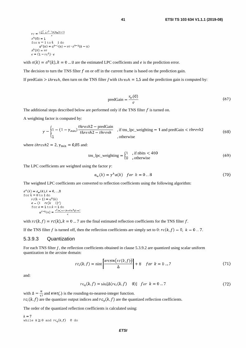
ETSI
ETSI TS 103 634 V1.1.1 (2019-08)41
�� =�∑ ������������
������
�
��0� = 1
for � = 1 to � − 1 do
���� = ������ + �� ∙ ����� − ��
���� = ��
� = �1 − �� � ∙ �
with ���� = ����, � = 0 … 8 are the estimated LPC coefficients and � is the prediction error.
The decision to turn the TNS filter � on or off in the current frame is based on the prediction gain.
If predGain > �ℎ���ℎ, then turn on the TNS filter �with �ℎ���ℎ = 1,5 and the prediction gain is computed by:
predGain =��0�� �67�
The additional steps described below are performed only if the TNS filter � is turned on.
A weighting factor is computed by:
� = �1 − �1 − ����� �ℎ���ℎ2 − predGain�ℎ���ℎ2 − �ℎ���ℎ, if tns_lpc_weighting = 1 and predGain < �ℎ���ℎ2
1 , otherwise �68�
where �ℎ���ℎ2 = 2, ���� = 0,85 and:
tns_lpc_weighting = �1 , if nbits < 480
0 , otherwise �69�
The LPC coefficients are weighted using the factor �: ���� = � ���� ��� � = 0 … 8 �70�
The weighted LPC coefficients are converted to reflection coefficients using the following algorithm:
����� = �����,� = 0, … ,8
for � = 8 to 1 do
���� − 1� = ����
� = �1 − ���� − 1� �
for � = 1 to � − 1 do
������ =�������������(��)
�
with ����, �� = �����, � = 0 … 7 are the final estimated reflection coefficients for the TNS filter �.
If the TNS filter � is turned off, then the reflection coefficients are simply set to 0: ����, �� = 0, � = 0 … 7.
5.3.9.3 Quantization
For each TNS filter �, the reflection coefficients obtained in clause 5.3.9.2 are quantized using scalar uniform quantization in the arcsine domain:
�����, �� = nint �arcsin�����, ���Δ
+ 8 ��� � = 0 … 7 �71�
and: �����, �� = sin!Δ������, �� − 8�" ��� � = 0 … 7 �72�
with Δ =�
�� and nint(.) is the rounding-to-nearest-integer function. �����, �� are the quantizer output indices and �����, �� are the quantized reflection coefficients.
The order of the quantized reflection coefficients is calculated using:
� = 7 while � ≥ 0 and �����,� = 0 do
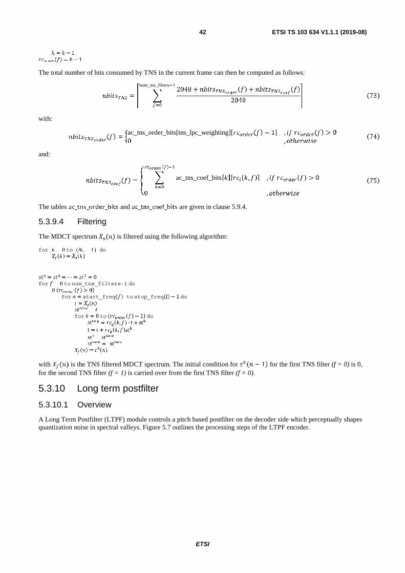
ETSI
ETSI TS 103 634 V1.1.1 (2019-08)42
� = � − 1 �����() = � + 1
The total number of bits consumed by TNS in the current frame can then be computed as follows:
�#������ = $ 2048 + �#�������������� + �#�������������2048
num_tns_filters��
���
% �73�
with:
�#�������������� = �ac_tns_order_bits[tns_lpc_weighting][���������� − 1] , �� ���������� > 0
0 , ��ℎ������ �74�
and:
�#������������� = & ac_tns_coef_bits!�"!�����, ��"������������
��
, �� ���������� > 0
0 , ��ℎ������ �75�
The tables ac_tns_order_bits and ac_tns_coef_bits are given in clause 5.9.4.
5.3.9.4 Filtering
The MDCT spectrum ��(�) is filtered using the following algorithm:
for � = 0 to (� − 1) do ����� = �����
� � = � � = ⋯ = � � = 0
for = 0 to num_tns_filters-1 do
if �������� > 0�
for � = start_freq�� to stop_freq�f� − 1 do
= ����� � ���� =
for � = 0 to �������� − 1� do st��� = �����,� ∙ t + st�
t = t + �����,�st�
st� = st���� st���� = st���
����� = (�)
with ��(�) is the TNS filtered MDCT spectrum. The initial condition for � �� − 1� for the first TNS filter (f = 0) is 0, for the second TNS filter (f = 1) is carried over from the first TNS filter (f = 0).
5.3.10 Long term postfilter
5.3.10.1 Overview
A Long Term Postfilter (LTPF) module controls a pitch based postfilter on the decoder side which perceptually shapes quantization noise in spectral valleys. Figure 5.7 outlines the processing steps of the LTPF encoder.
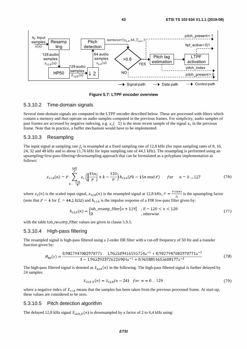
ETSI
ETSI TS 103 634 V1.1.1 (2019-08)43
Figure 5.7: LTPF encoder overview
5.3.10.2 Time-domain signals
Several time-domain signals are computed in the LTPF encoder described below. These are processed with filters which contain a memory and thus operate on audio samples computed in the previous frames. For simplicity, audio samples of past frames are accessed by negative indexing, e.g. '��−1� is the most recent sample of the signal '� in the previous frame. Note that in practice, a buffer mechanism would have to be implemented.
5.3.10.3 Resampling
The input signal at sampling rate �� is resampled at a fixed sampling rate of 12,8 kHz (for input sampling rates of 8, 16, 24, 32 and 48 kHz and to about 11,76 kHz for input sampling rate of 44,1 kHz). The resampling is performed using an upsampling+low-pass-filtering+downsampling approach that can be formulated as a polyphase implementation as follows:
'��.��� = ( '� )*15�( + + � −120( , ℎ��.�(� − 15� mod (�
����
������
��� � = 0 … 127 �76�
where '�(�) is the scaled input signal, '��.(�) is the resampled signal at 12,8 kHz, ( =��� ��
�� is the upsampling factor
(note that ( = 4 for �� = 44,1 �-.) and ℎ��. is the impulse response of a FIR low-pass filter given by:
ℎ��.��� = �tab_resamp_filter!� + 119" , if − 120 < � < 120
0 , otherwise �77�
with the table tab_resamp_filter values are given in clause 5.9.5.
5.3.10.4 High-pass filtering
The resampled signal is high-pass filtered using a 2-order IIR filter with a cut-off frequency of 50 Hz and a transfer function given by:
-���.� =0,9827947082978771 − 1,965589416595754.�� + 0,9827947082978771.��
1 − 1,9652933726226904.�� + 0,9658854605688177.�� �78�
The high-pass filtered signal is denoted as '/��.��� in the following. The high-pass filtered signal is further delayed by 24 samples: '/��._ ��� = '/��.�� − 24� ��� � = 0 … 129 �79�
where a negative index of '/��. means that the samples has been taken from the previous processed frame. At start-up, these values are considered to be zero.
5.3.10.5 Pitch detection algorithm
The delayed 12,8 kHz signal '/��._ (�) is downsampled by a factor of 2 to 6,4 kHz using:
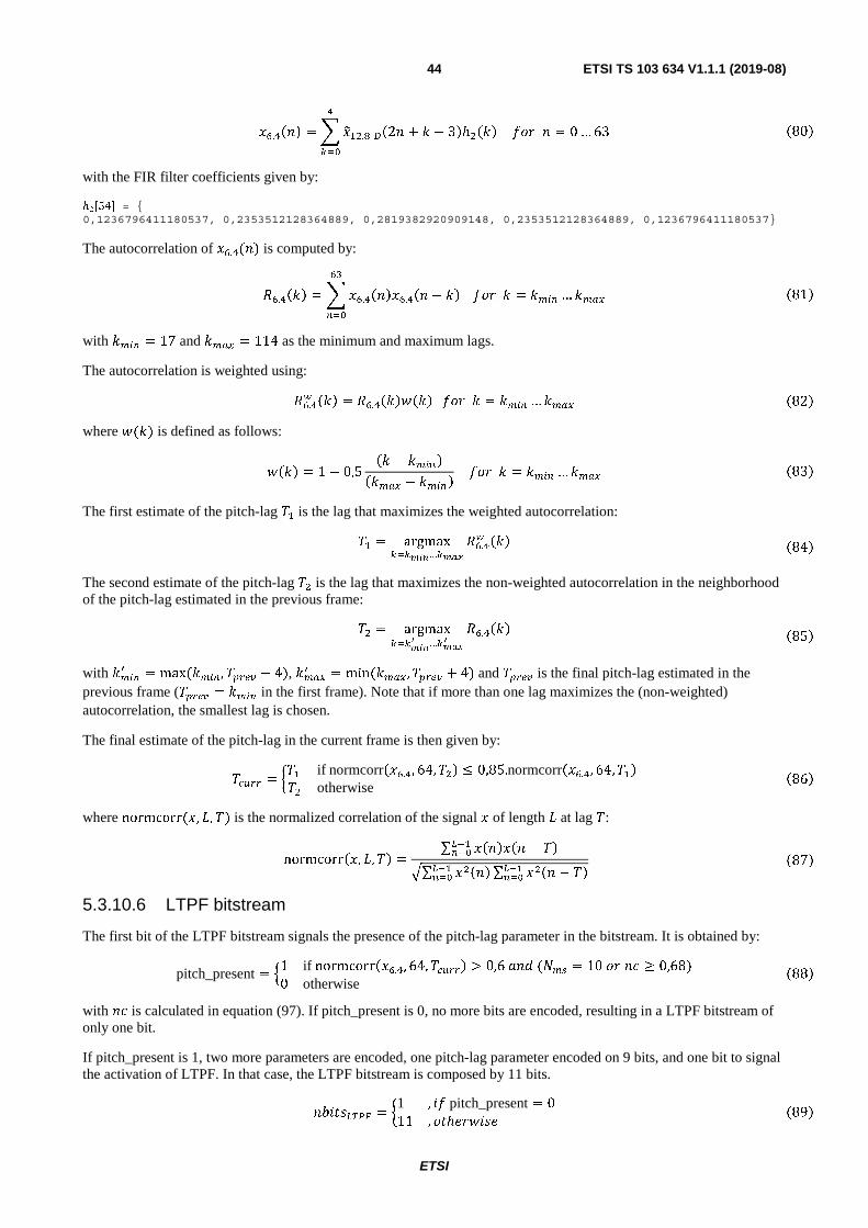
ETSI
ETSI TS 103 634 V1.1.1 (2019-08)44
'!."��� = '/��._ �2� + � − 3�ℎ����"
��
��� � = 0 … 63 �80�
with the FIR filter coefficients given by:
ℎ [54] = { 0,1236796411180537, 0,2353512128364889, 0,2819382920909148, 0,2353512128364889, 0,1236796411180537}
The autocorrelation of '!."(�) is computed by:
0!."��� = '!."���'!."�� − �� ��� � = ���� … ��#$!%
���
�81�
with ���� = 17 and ��#$ = 114 as the minimum and maximum lags.
The autocorrelation is weighted using: 0!." ��� = 0!."������� ��� � = ���� … ��#$ �82�
where �(�) is defined as follows:
���� = 1 − 0,5�� − ��������#$ − ����� ��� � = ���� … ��#$ �83�
The first estimate of the pitch-lag 1� is the lag that maximizes the weighted autocorrelation: 1� = argmax � �… ���
0!." ��� �84�
The second estimate of the pitch-lag 1� is the lag that maximizes the non-weighted autocorrelation in the neighborhood of the pitch-lag estimated in the previous frame: 1� = argmax
� �
… ���
0!."��� �85�
with ����& = max (���� , 1'��( − 4), ��#$& = min (��#$ , 1'��( + 4) and 1'��( is the final pitch-lag estimated in the previous frame (1'��( = ���� in the first frame). Note that if more than one lag maximizes the (non-weighted) autocorrelation, the smallest lag is chosen.
The final estimate of the pitch-lag in the current frame is then given by:
1�)�� = �1� if normcorr�'!.", 64, 1�� ≤ 0,85.normcorr�'!.", 64, 1��1� otherwise
�86�
where normcorr(', 2, 1) is the normalized correlation of the signal ' of length 2 at lag 1:
normcorr�', 2, 1� =∑ '���'�� − 1�*�����3∑ '����*��
��� ∑ '��� − 1�*�����
�87�
5.3.10.6 LTPF bitstream
The first bit of the LTPF bitstream signals the presence of the pitch-lag parameter in the bitstream. It is obtained by:
pitch_present = 41 if normcorr�'!.", 64, 1�)��� > 0,6 ��5 (6�� = 10 �� �� ≥ 0,68)
0 otherwise �88�
with �� is calculated in equation (97). If pitch_present is 0, no more bits are encoded, resulting in a LTPF bitstream of only one bit.
If pitch_present is 1, two more parameters are encoded, one pitch-lag parameter encoded on 9 bits, and one bit to signal the activation of LTPF. In that case, the LTPF bitstream is composed by 11 bits.
�#���*��+ = �1 , �� pitch_present = 0
11 , ��ℎ������ �89�

ETSI
ETSI TS 103 634 V1.1.1 (2019-08)45
The pitch-lag parameter and the activation bit are obtained as described in the following clauses.
5.3.10.7 LTPF pitch-lag parameter
The integer part of the LTPF pitch-lag parameter is given by:
pitch_int = argmax � �
… ���
0��.��� �90�
with:
0��.��� = '/��._ ���'/��._ �� − �����
���
��� � = (����&& − 4) … (��#$&& + 4) �91�
and ����&& = max (32, 21�)�� − 4), ��#$&& = min (228, 21�)�� + 4).
The fractional part of the LTPF pitch-lag is then given by:
pitch_fr =
⎩⎪⎨⎪⎧0 if pitch_int ≥ 157
argmax����,�,�
�����7�5� if 157 > pitch_int ≥ 127
argmax���%…%
�����7�5� if 127 > pitch_int>32
argmax���…%
�����7�5� if pitch_int = 32
�92�
with:
�����7�5� = 0��.�pitch_int + 8�ℎ"�48 − 5�"
���"
, �93�
5 being an array of pre-defined indices dependent on pitch_int and ℎ" is the impulse response of a FIR low-pass filter given by:
ℎ"��� = �tab_ltpf_interp_R�� + 15� , if − 16 < � < 16
0 , otherwise �94�
with tab_ltpf_interp_R is provided by table 5.42 in clause 5.9.5.
If pitch_fr < 0 then both pitch_int and pitch_fr are modified according to:
pitch_int = pitch_int − 1
pitch_fr = pitch_fr + 4 �95�
Finally, the pitch-lag parameter index is given by:
pitch_index = &pitch_int + 283 if pitch_int ≥ 157
2 ∗ pitch_int +pitch_fr
2+ 126 if 157 > pitch_int ≥ 127
4 ∗ pitch_int + pitch_fr − 128 if 127 > pitch_int
�96�
5.3.10.8 LTPF activation bit
A normalized correlation is first computed as follows:
�� =∑ '���, 0�'��� − pitch_int, −pitch_fr�������3∑ '����, 0����
��� ∑ '���� − pitch_int, −pitch_fr�������
�97�
with:
'���, 5� = '/��,_ �� + ��ℎ��4� − 5��
���
�98�

ETSI
ETSI TS 103 634 V1.1.1 (2019-08)46
and ℎ� is the impulse response of a FIR low-pass filter given by:
ℎ���� = �tab_ltpf_interp_x12k8�� + 7� , if − 8 < � < 8
0 , otherwise �99�
with tab_ltpf_interp_x12k8 is given in clause 5.9.5.
The LTPF activation bit is then set according to:
if ( (mem_ltpf_active==0 && (!� == 10 || mem_mem_nc > 0.94) && mem_nc>0.94 && nc>0.94) || (mem_ltpf_active==1 && nc>0.9) || (mem_ltpf_active==1 && abs(pitch-mem_pitch)<2 && (nc-mem_nc)>-0.1 && nc>0.84) ) { ltpf_active = 1; } else { ltpf_active = 0; }
where mem_ltpf_active is the value of ltpf_active in the previous frame (it is 0 if pitch_present = 0 in the previous frame), mem_nc is the value of nc in the previous frame (it is 0 if pitch_present = 0 in the previous frame), mem_mem_nc is the value of nc in the penultimate frame, pitch = pitch_int+pitch_fr/4 and mem_pitch is the value of pitch in the previous frame (it is 0 if pitch_present = 0 in the previous frame).
5.3.11 Spectral quantization
5.3.11.1 Overview
The MDCT spectrum after TNS filtering (��(�), see clause 5.3.9.4) is quantized using dead-zone plus uniform threshold scalar quantization and the quantized MDCT spectrum ����� is then encoded using arithmetic encoding. A global gain 99 controls the step size of the quantizer. This global gain is quantized with 8 bits and the quantized global gain index 99��� is then an integer between 0 and 255. The global gain index is chosen such that the number of bits needed to encode the quantized MDCT spectrum is as close as possible to the available bit budget.
5.3.11.2 Bit budget
The number of bits available for coding the spectrum is given by: �#����'�� = �#��� − �#���, − �#������ − �#���*��+ − �#������ − �#���-#�� − �#����� − �#���#�� �100�
with �#��� given in clause 5.2.5, �#���, given in clause 5.3.5, �#������ given in clause 5.3.9.3, �#���*��+ given in clause 5.3.10.6, �#������ = 38, �#���-#�� = 8, �#����� = 3 and:
�#���#�� =
⎩⎪⎨⎪⎧:log� )6.
2,; + 3 , if �#��� ≤ 1280
:log� )6.2
,; + 4 , if 1280 < �#��� ≤ 2560
:log� )6.2
,; + 5 , otherwise
�101�
5.3.11.3 First global gain estimation
An offset is first computed using:
�#��������/ = �0,8 ∗ �#��������/�0� + 0,2 ∗ min�40, max�−40, �#��������/�0� + �#����'���0� − �#�����/�0��� , if ����������/�0� = 0
0 , otherwise �102�
with �#��������/�0� is the value of �#��������/ in the previous frame, �#����'���0� is the value of �#����'�� in the previous frame, �#�����/�0� is the value of �#�����/ in the previous frame (�#�����/ is computed in clause 5.3.11.5) and ����������/�0� is the value of ����������/ in the previous frame (����������/ is computed at the end of the current clause). Note that �#��������/�0� , �#����'���0� , �#�����/�0� and ����������/�0� are all initialized to zero before the first frame is processed. If the spectrum was re-quantized in the previous frame, �#��������/�0� , �#����'���0� ��5 ����������/�0� refer to the values prior to re-quantization.
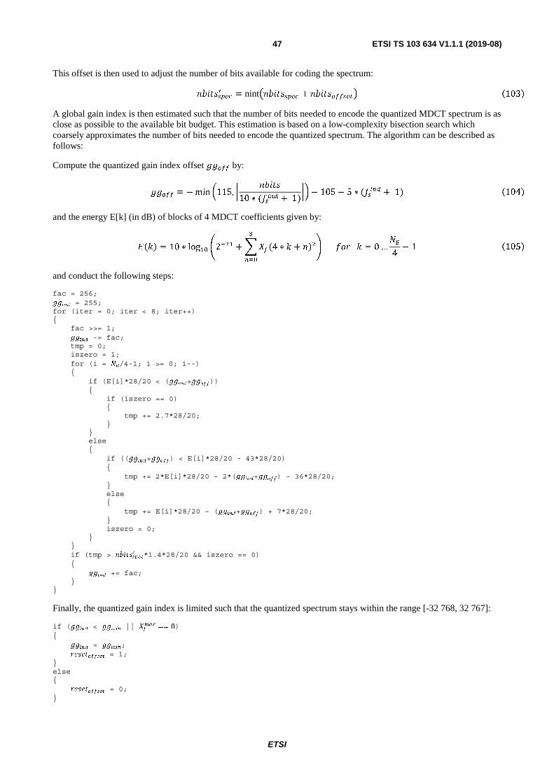
ETSI
ETSI TS 103 634 V1.1.1 (2019-08)47
This offset is then used to adjust the number of bits available for coding the spectrum:
�#����'��& = nint��#����'�� + �#��������/� �103�
A global gain index is then estimated such that the number of bits needed to encode the quantized MDCT spectrum is as close as possible to the available bit budget. This estimation is based on a low-complexity bisection search which coarsely approximates the number of bits needed to encode the quantized spectrum. The algorithm can be described as follows:
Compute the quantized gain index offset 99��� by:
99��� = − min )115, * �#���10 ∗ (����� + 1)
+, − 105 − 5 ∗ (����� + 1) �104�
and the energy E[k] (in dB) of blocks of 4 MDCT coefficients given by:
<��� = 10 ∗ log�� =2�%� + ���4 ∗ � + ���%
���
> ��� � = 0 …6.4
− 1 �105�
and conduct the following steps:
fac = 256; ��"�� = 255; for (iter = 0; iter < 8; iter++) { fac >>= 1; ��"�� -= fac; tmp = 0; iszero = 1; for (i = �/4-1; i >= 0; i--) { if (E[i]*28/20 < (��"��+�����)) { if (iszero == 0) { tmp += 2.7*28/20; } } else { if ((��"��+�����) < E[i]*28/20 - 43*28/20) { tmp += 2*E[i]*28/20 – 2*(��"��+�����) - 36*28/20; } else { tmp += E[i]*28/20 – (��"��+�����) + 7*28/20; } iszero = 0; } } if (tmp > ��� ��#��
$ *1.4*28/20 && iszero == 0) { ��"�� += fac; } }
Finally, the quantized gain index is limited such that the quantized spectrum stays within the range [-32 768, 32 767]:
if (��"�� < ��!"� || ��!�% == 0)
{ ��"�� = ��!"�; ���� �����& = 1; } else { ���� �����& = 0; }

ETSI
ETSI TS 103 634 V1.1.1 (2019-08)48
with:
99��� = ?@28 ∗ log10 A ���#$32768 − 0.375
BC − 99��� , if ���#$ > 0
0 , otherwise
�106�
and:
���#$ = max�1�2��
D�����D �107�
5.3.11.4 Quantization
The quantized global gain index found in clause 5.3.11.3 is first unquantized using:
99 = 10--�3--���
� �108�
The spectrum �� is then quantized using:
����� =
⎩⎪⎨⎪⎧E�����99 + 0.375F , if ����� ≥ 0
@�����99 − 0.375C , otherwise
��� � = 0 … 6. − 1 �109�
5.3.11.5 Bit consumption
The number of bits �#�����/ needed to encode the quantized MDCT spectrum ����� can be accurately estimated using the algorithm below.
Two bitrate flags are first computed using:
if (nbits > (160 + �"�� * 160))
{ rateFlag = 512; } else { rateFlag = 0; } if (nbits >= (480 + �
"�� * 160)) { modeFlag = 1; } else { modeFlag = 0; }
Then the index of the last non-zeroed 2-tuple is obtained by:
lastnz = �; while (lastnz>2 && ��[lastnz-1] == 0 && ��[lastnz-2] == 0) { lastnz -= 2; }
The number of bits �#�����/ is then computed as follows:
��� ���& = 0; ��� �&'�� = 0; ��� �(�) = 0; lastnz_trunc = 2; c = 0; for (n = 0; n < lastnz; n=n+2) { t = c + rateFlag; if (n > �/2) { t += 256;

ETSI
ETSI TS 103 634 V1.1.1 (2019-08)49
} a = abs(��[n]); b = abs(��[n+1]); lev = 0; while (max(a,b) >= 4) { pki = ac_spec_lookup[t+lev*1024]; ��� ���& += ac_spec_bits[pki][16]; if (lev == 0 && modeFlag == 1) { ��� �(�) += 2; } else { ��� ���& += 2*2048; } a >>= 1; b >>= 1; lev = min(lev+1,3); } pki = ac_spec_lookup[t+lev*1024]; sym = a + 4*b; ��� ���& += ac_spec_bits[pki][sym]; a_lsb = abs(��[n]); b_lsb = abs(��[n+1]); ��� ���& += (min(a_lsb,1) + min(b_lsb,1)) * 2048; if (lev > 0 && modeFlag == 1) { a_lsb >>= 1; b_lsb >>= 1; if (a_lsb == 0 && ��[n] != 0) { ��� �(�)++; } if (b_lsb == 0 && ��[n+1] != 0) { ��� �(�)++; } } ��� ���& += (min(a,1) + min(b,1)) * 2048; if ((��[n] != 0 || ��[n+1] != 0) && (��� ���& <= ��� ��#��*2048)) { lastnz_trunc = n + 2; ��� �&'�� = ��� ���&; } if (lev <= 1) { t = 1 + (a+b)*(lev+1); } else { t = 12 + lev; } c = (c&15)*16 + t; } ��� ���& = ceil(��� ���&/2048) + ��� �(�); ��� �&'�� = ceil(��� �&'��/2048);
with ac_lookup and ac_bits determined by the tables given in clause 5.9.6, Table 5.43.
5.3.11.6 Truncation
The quantized spectrum is truncated such that the number of bits needed to encode it is within the available bit budget.
for (k = lastnz_trunc; k < lastnz; k++) { ��[k] = 0; }
with lastnz and lastnz_trunc given in clause 5.3.11.5.
A flag which allows the truncation of the LSBs in the arithmetic encoding/decoding is obtained using:
if (modeFlag == 1 && ��� ���& > ��� ��#��)
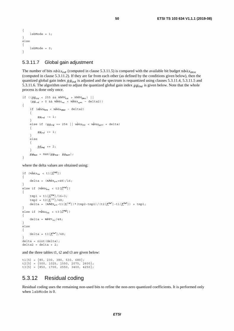
ETSI
ETSI TS 103 634 V1.1.1 (2019-08)50
{ lsbMode = 1; } else { lsbMode = 0; }
5.3.11.7 Global gain adjustment
The number of bits �#�����/ (computed in clause 5.3.11.5) is compared with the available bit budget �#����'�� (computed in clause 5.3.11.2). If they are far from each other (as defined by the conditions given below), then the quantized global gain index 99��� is adjusted and the spectrum is requantized using clauses 5.3.11.4, 5.3.11.5 and 5.3.11.6. The algorithm used to adjust the quantized global gain index 99��� is given below. Note that the whole process is done only once.
if ((��"�� < 255 && ��� ���& > ��� ��#��) || (��"�� > 0 && ��� ���& < ��� ��#�� – delta2)) { if (��� ���& < ��� ��#�� – delta2) { ��"�� -= 1; } else if (��"�� == 254 || ��� ���& < ��� ��#�� + delta) { ��"�� += 1; } else { ��"�� += 2; } ��"�� = max(��"��, ��!"�); }
where the delta values are obtained using:
if (��� ���& < t1[�"��])
{ delta = (��� ���&+48)/16; } else if (��� ���& < t2[�
"��]) { tmp1 = t1[�
"��]/16+3; tmp2 = t2[�
"��]/48; delta = (��� ���&-t1[�
"��])*(tmp2-tmp1)/(t2[�"��]-t1[�
"��]) + tmp1; } else if (��� ���& < t3[�
"��]) { delta = ��� ���&/48; } else { delta = t3[�
"��]/48; } delta = nint(delta); delta2 = delta + 2;
and the three tables t1, t2 and t3 are given below:
t1[5] = {80, 230, 380, 530, 680}; t2[5] = {500, 1025, 1550, 2075, 2600}; t3[5] = {850, 1700, 2550, 3400, 4250};
5.3.12 Residual coding
Residual coding uses the remaining non-used bits to refine the non-zero quantized coefficients. It is performed only when lsbMode is 0.
ETSI
ETSI TS 103 634 V1.1.1 (2019-08)51
Firstly, the maximum number of bits available for residual coding is calculated using:
nbits_residual_max = ��� ��#�� - ��� �&'�� + 4;
Then, the residual bits are computed using:
k = 0; nbits_residual = 0; while (k < � && nbits_residual < nbits_residual_max) { if (��[k] != 0) { if (��[k] >= ��[k]*gg) { res_bits[nbits_residual] = 1; } else { res_bits[nbits_residual] = 0; } nbits_residual++; } k++; }
5.3.13 Noise level estimation
5.3.13.1 Overview
The noise level estimator controls the noise filling on decoder side. On encoder side, the noise level parameter is estimated, quantized and transmitted in the bit stream.
5.3.13.2 Relevant spectral lines
The noise level is estimated based on the spectral coefficients which have been quantized to zero, i.e. ����� == 0. The indices for the relevant spectral coefficients are given by:
G�+��� = �1 if 6H�/#�/ ≤ � < #��/�' ��5 ����� == 0 ��� �II � = � − 6H��/4 … min�#�_���7, � + 6H_��5�ℎ�0 otherwise
�110�
where #�_���7 depends on the bandwidth detected in clause 5.3.5 as defined in Table 5.16.
Table 5.16: Mapping table ��_���� according to bandwidth
Bandwidth (���) NB WB SSWB SWB FB
��_���� 8 ∙ ��� 16 ∙ ��� 24 ∙ ��� 32 ∙ ��� ��
The tuning parameters ��_�� and ��_ ��ℎ are given in Table 5.17.
Table 5.17: Tuning table for noise level estimation
�� _�� �� _����� 2,5 6 1 5 12 1
10 24 3

ETSI
ETSI TS 103 634 V1.1.1 (2019-08)52
5.3.13.3 Noise level calculation
For the identified indices, the mean level of the missing coefficients is estimated based on the spectrum after TNS filtering (��(�), see clause 5.3.9.4) and normalized by the global gain. If nbytes is larger than 20 or if the frame length is not 10 ms, the noise level is calculated as:
��� =
∑ ������ ∙���������
����
���∑ ����������
���
�111�
where � is defined in clause 5.3.4.3. Otherwise, if the frame length is 10 ms and nbytes equals 20, two noise levels are calculated over the upper and lower half of the relevant spectral lines. To this end, a split point �� is calculated as the mean value of the relevant spectral lines, i.e.:
�� =∑ ����� ∙�����
���∑ ����� ����
��� .
The two noise levels are then computed as:
���� =∑ ����� ∙
��� ��
��
���∑ ����� ��
���
and:
���� =∑ ����� ∙
��� ��
����
������∑ ����� ����
������
and the final noise level is calculated as ��� = min�����, �����. The final noise level is quantized to eight steps:
��� = �������� ⌊8 − 16 ∙ ���⌉, 0�, 7� �112� 5.3.14 Bitstream encoding
5.3.14.1 Overview
The bitstream of an encoded audio frame consists of the four parts:
• initial side information
• a dynamic data block for which is arithmetically coded
• a dynamic data block with signs and least significant bits of the encoded spectrum
• residual data
An overview on the bitstream structure and layout is provided in clause 5.5. The following clauses define the exact payload writing process of all codec elements.
5.3.14.2 Initialization
bp = 0; bp_side = nbytes – 1; mask_side = 1; c = 0; nlsbs = 0;
ETSI
ETSI TS 103 634 V1.1.1 (2019-08)53
5.3.14.3 Side information
/* Bandwidth */ if (������� > 0) { write_uint_backward(bytes, &bp_side, &mask_side, ���, �������); } /* Last non-zero tuple */ write_uint_backward(bytes, &bp_side, &mask_side, (lastnz_trunc >> 1) - 1, ceil(log2(��/2))); /* LSB mode bit */ write_bit_backward(bytes, &bp_side, &mask_side, lsbMode); /* Global Gain */ write_uint_backward(bytes, &bp_side, &mask_side, �����, 8); /* TNS activation flag */ for (f = 0; f < num_tns_filters; f++) { write_bit_backward(bytes, &bp_side, &mask_side, min(������ , 1)); } /* Pitch present flag */ write_bit_backward(bytes, &bp_side, &mask_side, pitch_present); /* Encode SCF VQ parameters - 1st stage (10 bits) */ write_uint_backward(bytes, &bp_side, &mask_side, ind_LF, 5); write_uint_backward(bytes, &bp_side, &mask_side, ind_HF, 5); /* Encode SCF VQ parameters - 2nd stage side-info (3-4 bits) */ write_bit_backward(bytes, &bp_side, &mask_side, shape_j>>1 ) submode_LSB = (shape_j & 0x1); /* shape_j is the stage2 shape_index [0…3] */ submode_MSB = (shape_j>>1); gain_MSBs = gain_i; /* where gain_i is the SNS-VQ stage 2 gain_index */ gain_MSBs = (gain_MSBs >> sns_gainLSBbits[shape_j]); write_uint_backward(bytes,&bp_side,&mask_side,gain_MSBs, sns_gainMSBbits[shape_j]); write_bit_backward(bytes, &bp_side, &mask_side, LS_indA); /* Encode SCF VQ parameters - 2nd stage MPVQ data */ if (submode_MSB == 0) { if (submode_LSB == 0) { tmp = index_joint_0; /* Eq. 55 */ } else { tmp = index_joint_1; /* Eq. 56 */ } write_uint_backward(bytes, &bp_side, &mask_side, tmp, 13) write_uint_backward(bytes, &bp_side, &mask_side, tmp>>13, 12); } else { if (submode_LSB == 0) { tmp = index_joint_2; /* Eq. 57 */ } else { tmp = index_joint_3; /* Eq. 58 */ } write_uint_backward(bytes, &bp_side, &mask_side, tmp, 12); write_uint_backward(bytes, &bp_side, &mask_side, tmp>> 12, 12); } /* LTPF data */ if (pitch_present != 0) { write_uint_backward(bytes, &bp_side, &mask_side, ltpf_active, 1); write_uint_backward(bytes, &bp_side, &mask_side, pitch_index, 9); } /* Noise Factor */ write_uint_backward(bytes, &bp_side, &mask_side, ��, 3);
5.3.14.4 Arithmetic encoding
5.3.14.4.1 Overview
The TNS data (if TNS is active) and the quantized spectral coefficients �� are noiselessly encoded. �� is encoded starting from the lowest-frequency coefficient, progressing to the highest-frequency coefficient. They are encoded by groups of two coefficients a and b resulting in a so-called 2-tuple {a, b}.
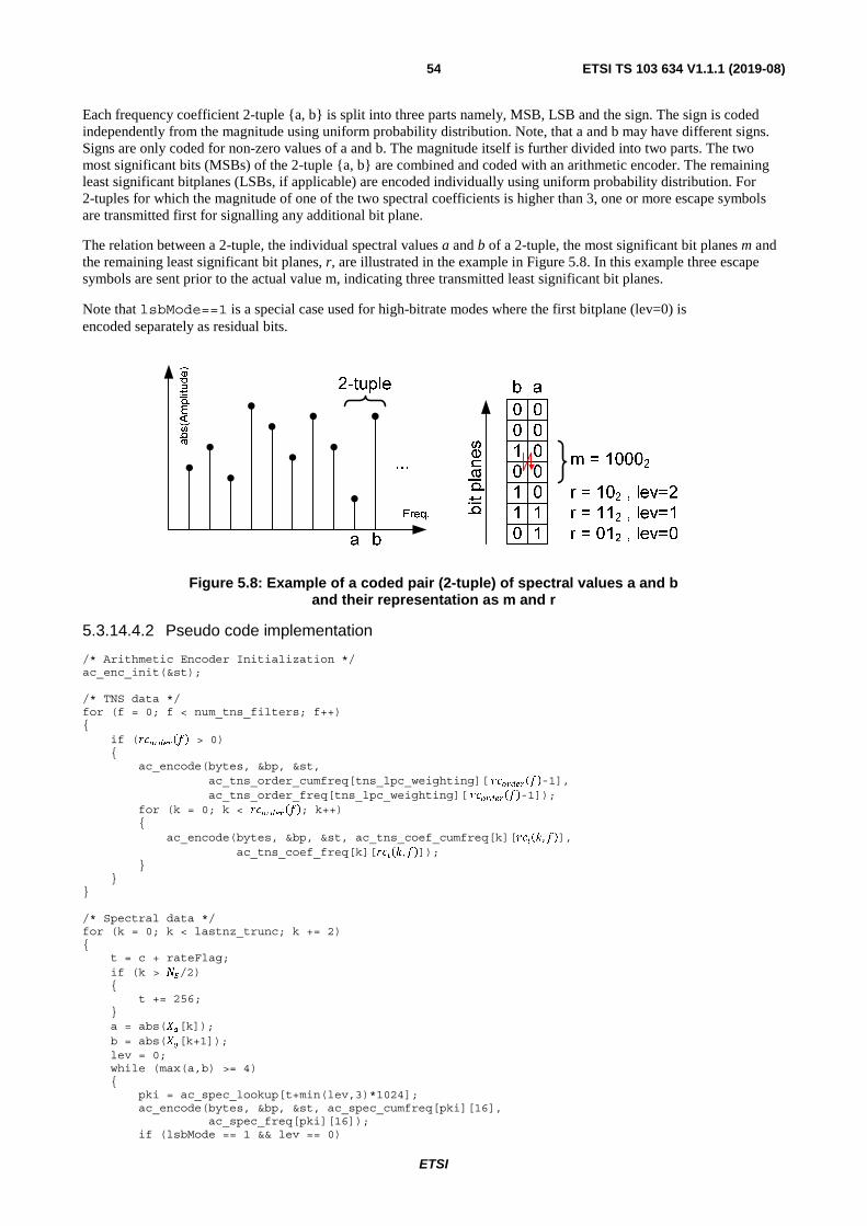
ETSI
ETSI TS 103 634 V1.1.1 (2019-08)54
Each frequency coefficient 2-tuple {a, b} is split into three parts namely, MSB, LSB and the sign. The sign is coded independently from the magnitude using uniform probability distribution. Note, that a and b may have different signs. Signs are only coded for non-zero values of a and b. The magnitude itself is further divided into two parts. The two most significant bits (MSBs) of the 2-tuple {a, b} are combined and coded with an arithmetic encoder. The remaining least significant bitplanes (LSBs, if applicable) are encoded individually using uniform probability distribution. For 2-tuples for which the magnitude of one of the two spectral coefficients is higher than 3, one or more escape symbols are transmitted first for signalling any additional bit plane.
The relation between a 2-tuple, the individual spectral values a and b of a 2-tuple, the most significant bit planes m and the remaining least significant bit planes, r, are illustrated in the example in Figure 5.8. In this example three escape symbols are sent prior to the actual value m, indicating three transmitted least significant bit planes.
Note that lsbMode==1 is a special case used for high-bitrate modes where the first bitplane (lev=0) is encoded separately as residual bits.
Figure 5.8: Example of a coded pair (2-tuple) of spectral values a and b and their representation as m and r
5.3.14.4.2 Pseudo code implementation
/* Arithmetic Encoder Initialization */ ac_enc_init(&st); /* TNS data */ for (f = 0; f < num_tns_filters; f++) { if (������ > 0) { ac_encode(bytes, &bp, &st, ac_tns_order_cumfreq[tns_lpc_weighting][ ������ -1], ac_tns_order_freq[tns_lpc_weighting][ ������ -1]); for (k = 0; k < ������ ; k++) { ac_encode(bytes, &bp, &st, ac_tns_coef_cumfreq[k][���,� ], ac_tns_coef_freq[k][���,� ]); } } } /* Spectral data */ for (k = 0; k < lastnz_trunc; k += 2) { t = c + rateFlag; if (k > ��/2) { t += 256; } a = abs(��[k]); b = abs(��[k+1]); lev = 0; while (max(a,b) >= 4) { pki = ac_spec_lookup[t+min(lev,3)*1024]; ac_encode(bytes, &bp, &st, ac_spec_cumfreq[pki][16], ac_spec_freq[pki][16]); if (lsbMode == 1 && lev == 0)
abs(Amplitude)
ETSI
ETSI TS 103 634 V1.1.1 (2019-08)55
{ lsb0 = a & 1; lsb1 = b & 1; } else { write_bit_backward(bytes, &bp_side, &mask_side, a & 1); write_bit_backward(bytes, &bp_side, &mask_side, b & 1); } a >>= 1; b >>= 1; lev++; } pki = ac_spec_lookup[t+min(lev,3)*1024]; sym = a + 4*b; ac_encode(bytes, &bp, &st, ac_spec_cumfreq[pki][sym], ac_spec_freq[pki][sym]); a_lsb = abs(��[k]); b_lsb = abs(��[k+1]); if (lsbMode == 1 && lev > 0) { a_lsb >>= 1; b_lsb >>= 1; lsbs[nlsbs++] = lsb0; if (a_lsb == 0 && ��[k] != 0) { lsbs[nlsbs++] = ��[k]>0?0:1; } lsbs[nlsbs++] = lsb1; if (b_lsb == 0 && ��[k+1] != 0) { lsbs[nlsbs++] = ��[k+1]>0?0:1; } } if (a_lsb > 0) { write_bit_backward(bytes, &bp_side, &mask_side, ��[k]>0?0:1); } if (b_lsb > 0) { write_bit_backward(bytes, &bp_side, &mask_side, ��[k+1]>0?0:1); } lev = min(lev,3); if (lev <= 1) { t = 1 + (a+b)*(lev+1); } else { t = 12 + lev; } c = (c&15)*16 + t; }
5.3.14.5 Residual data and finalization
/* Residual bits */ nbits_side = nbits – (8 * bp_side + 8 – log2(mask_side)); nbits_ari = bp * 8; nbits_ari += 25 – floor(log2(st->range)); if (st->cache >= 0) { nbits_ari += 8; } if (st->carry_count > 0) { nbits_ari += st->carry_count * 8; } nbits_residual_enc = nbits – (nbits_side + nbits_ari); if (lsbMode == 0) { nbits_residual_enc = min(nbits_residual_enc, nbits_residual); for (k = 0; k < nbits_residual_enc; k++) { write_bit_backward(bytes, &bp_side, &mask_side, res_bits[k]); } }
ETSI
ETSI TS 103 634 V1.1.1 (2019-08)56
else { nbits_residual_enc = min(nbits_residual_enc, nlsbs); for (k = 0; k < nbits_residual_enc; k++) { write_bit_backward(bytes, &bp_side, &mask_side, lsbs[k]); } } /* Arithmetic Encoder Finalization */ ac_enc_finish(bytes, &bp, &st);
where res_bits and nbits_residual are given in clause 5.3.12.
5.3.14.6 Functions
write_bit_backward(bytes[], *bp, *mask, bit) { if (bit == 0) { bytes[*bp] &= ~*mask; } else { bytes[*bp] |= *mask; } if (*mask == 0x80) { *mask = 1; *bp -= 1; } else { *mask <<= 1; } } write_uint_backward(bytes[], *bp, *mask, val, numbits) { for (k = 0; k < numbits; k++) { bit = val & 1; write_bit_backward(bytes, bp, mask, bit); val >>= 1; } } write_uint_forward(bytes[], bp, val, numbits) { mask = 0x80; for (k = 0; k < numbits; k++) { bit = val & mask; if (bit == 0) { bytes[bp] &= ~mask; } else { bytes[bp] |= mask; } mask >>= 1; } } ac_enc_init(*st) { st->low = 0; st->range = 0x00ffffff; st->cache = -1; st->carry = 0; st->carry_count = 0; } ac_shift(bytes[], *bp, *st) { if (st->low < 0x00ff0000 || st->carry == 1)

ETSI
ETSI TS 103 634 V1.1.1 (2019-08)57
{ if (st->cache >= 0) { bytes[(*bp)++] = st->cache + st->carry; } while (st->carry_count > 0) { bytes[(*bp)++] = (st->carry + 0xff) & 0xff; st->carry_count -= 1; } st->cache = st->low >> 16; st->carry = 0; } else { st->carry_count += 1; } st->low <<= 8; st->low &= 0x00ffffff; } ac_encode(bytes[], *bp, *st, cum_freq, sym_freq) { r = st->range >> 10; st->low += r * cum_freq; if (st->low >> 24) { st->carry = 1; } st->low &= 0x00ffffff; st->range = r * sym_freq; while (st->range < 0x10000) { st->range <<= 8; ac_shift(bytes, bp, st); } } ac_enc_finish(bytes[], *bp, *st) { bits = 1; while ((st->range >> (24-bits)) == 0) { bits++; } mask = 0x00ffffff >> bits; val = st->low + mask; over1 = val >> 24; val &= 0x00ffffff; high = st->low + st->range; over2 = high >> 24; high &= 0x00ffffff; val = val & ~mask; if (over1 == over2) { if (val + mask >= high) { bits += 1; mask >>= 1; val = ((st->low + mask) & 0x00ffffff) & ~mask; } if (val < st->low) { st->carry = 1; } } st->low = val; for (; bits > 0; bits -= 8) { ac_shift(bytes, bp, st); } bits += 8; if (st->carry_count > 0) { bytes[(*bp)++] = st->cache; for (; st->carry_count > 1; st->carry_count--) { bytes[(*bp)++] = 0xff;
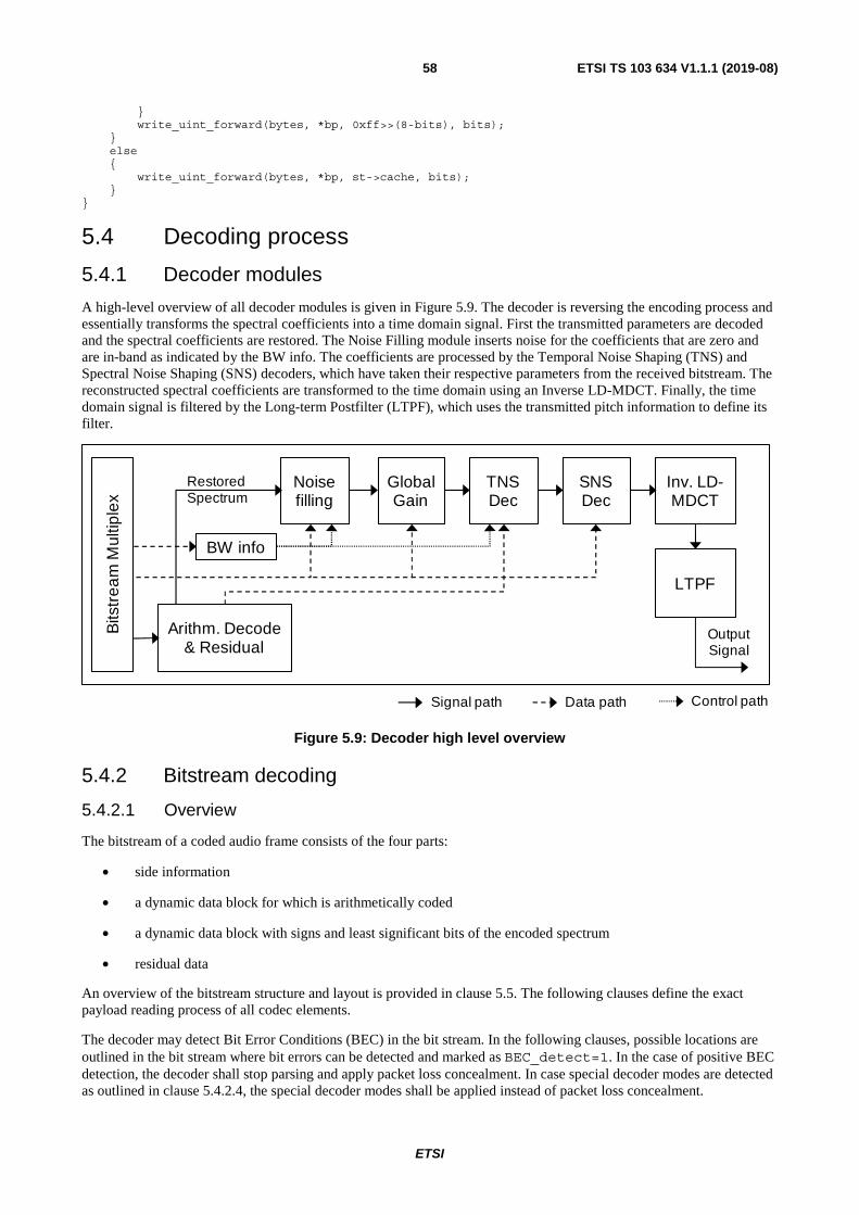
ETSI
ETSI TS 103 634 V1.1.1 (2019-08)58
} write_uint_forward(bytes, *bp, 0xff>>(8-bits), bits); } else { write_uint_forward(bytes, *bp, st->cache, bits); } }
5.4 Decoding process
5.4.1 Decoder modules
A high-level overview of all decoder modules is given in Figure 5.9. The decoder is reversing the encoding process and essentially transforms the spectral coefficients into a time domain signal. First the transmitted parameters are decoded and the spectral coefficients are restored. The Noise Filling module inserts noise for the coefficients that are zero and are in-band as indicated by the BW info. The coefficients are processed by the Temporal Noise Shaping (TNS) and Spectral Noise Shaping (SNS) decoders, which have taken their respective parameters from the received bitstream. The reconstructed spectral coefficients are transformed to the time domain using an Inverse LD-MDCT. Finally, the time domain signal is filtered by the Long-term Postfilter (LTPF), which uses the transmitted pitch information to define its filter.
Figure 5.9: Decoder high level overview
5.4.2 Bitstream decoding
5.4.2.1 Overview
The bitstream of a coded audio frame consists of the four parts:
• side information
• a dynamic data block for which is arithmetically coded
• a dynamic data block with signs and least significant bits of the encoded spectrum
• residual data
An overview of the bitstream structure and layout is provided in clause 5.5. The following clauses define the exact payload reading process of all codec elements.
The decoder may detect Bit Error Conditions (BEC) in the bit stream. In the following clauses, possible locations are outlined in the bit stream where bit errors can be detected and marked as BEC_detect=1. In the case of positive BEC detection, the decoder shall stop parsing and apply packet loss concealment. In case special decoder modes are detected as outlined in clause 5.4.2.4, the special decoder modes shall be applied instead of packet loss concealment.
Bits
trea
mM
ultip
lex
Inv. LD-MDCT
OutputSignal
SNS Dec
GlobalGain
Arithm. Decode & Residual
Noise filling
LTPF
TNS Dec
Restored Spectrum
BW info
Signal path Data path Control path
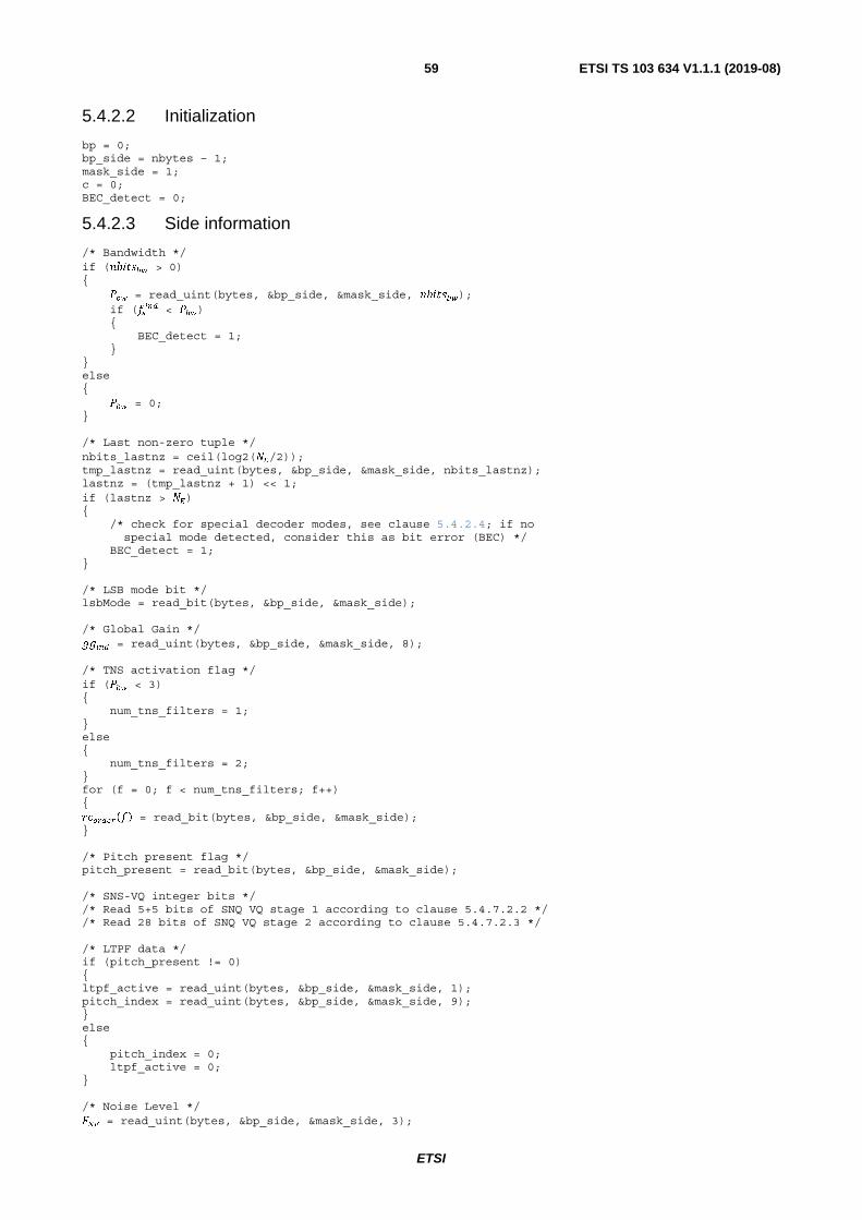
ETSI
ETSI TS 103 634 V1.1.1 (2019-08)59
5.4.2.2 Initialization
bp = 0; bp_side = nbytes – 1; mask_side = 1; c = 0; BEC_detect = 0;
5.4.2.3 Side information
/* Bandwidth */ if (������� > 0) { ��� = read_uint(bytes, &bp_side, &mask_side, �������); if (�
��� < ���) { BEC_detect = 1; } } else { ��� = 0; } /* Last non-zero tuple */ nbits_lastnz = ceil(log2(��/2)); tmp_lastnz = read_uint(bytes, &bp_side, &mask_side, nbits_lastnz); lastnz = (tmp_lastnz + 1) << 1; if (lastnz > ��) { /* check for special decoder modes, see clause 5.4.2.4; if no special mode detected, consider this as bit error (BEC) */ BEC_detect = 1; } /* LSB mode bit */ lsbMode = read_bit(bytes, &bp_side, &mask_side); /* Global Gain */ ����� = read_uint(bytes, &bp_side, &mask_side, 8); /* TNS activation flag */ if (��� < 3) { num_tns_filters = 1; } else { num_tns_filters = 2; } for (f = 0; f < num_tns_filters; f++) { ������ = read_bit(bytes, &bp_side, &mask_side); } /* Pitch present flag */ pitch_present = read_bit(bytes, &bp_side, &mask_side); /* SNS-VQ integer bits */ /* Read 5+5 bits of SNQ VQ stage 1 according to clause 5.4.7.2.2 */ /* Read 28 bits of SNQ VQ stage 2 according to clause 5.4.7.2.3 */ /* LTPF data */ if (pitch_present != 0) { ltpf_active = read_uint(bytes, &bp_side, &mask_side, 1); pitch_index = read_uint(bytes, &bp_side, &mask_side, 9); } else { pitch_index = 0; ltpf_active = 0; } /* Noise Level */ �� = read_uint(bytes, &bp_side, &mask_side, 3);
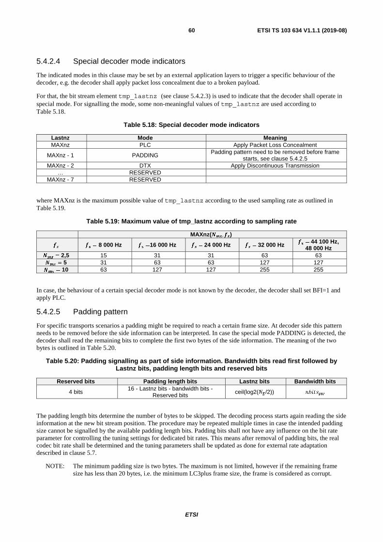
ETSI
ETSI TS 103 634 V1.1.1 (2019-08)60
5.4.2.4 Special decoder mode indicators
The indicated modes in this clause may be set by an external application layers to trigger a specific behaviour of the decoder, e.g. the decoder shall apply packet loss concealment due to a broken payload.
For that, the bit stream element tmp_lastnz (see clause 5.4.2.3) is used to indicate that the decoder shall operate in special mode. For signalling the mode, some non-meaningful values of tmp_lastnz are used according to Table 5.18.
Table 5.18: Special decoder mode indicators
Lastnz Mode Meaning MAXnz PLC Apply Packet Loss Concealment
MAXnz - 1 PADDING Padding pattern need to be removed before frame starts, see clause 5.4.2.5
MAXnz - 2 DTX Apply Discontinuous Transmission … RESERVED
MAXnz - 7 RESERVED
where MAXnz is the maximum possible value of tmp_lastnz according to the used sampling rate as outlined in Table 5.19.
Table 5.19: Maximum value of tmp_lastnz according to sampling rate
MAXnz(��, ��)
�� �� = 8 000 Hz �� =16 000 Hz �� = 24 000 Hz �� = 32 000 Hz �� = 44 100 Hz, 48 000 Hz
�� = 2,5 15 31 31 63 63 �� = 5 31 63 63 127 127 �� = 10 63 127 127 255 255
In case, the behaviour of a certain special decoder mode is not known by the decoder, the decoder shall set BFI=1 and apply PLC.
5.4.2.5 Padding pattern
For specific transports scenarios a padding might be required to reach a certain frame size. At decoder side this pattern needs to be removed before the side information can be interpreted. In case the special mode PADDING is detected, the decoder shall read the remaining bits to complete the first two bytes of the side information. The meaning of the two bytes is outlined in Table 5.20.
Table 5.20: Padding signalling as part of side information. Bandwidth bits read first followed by Lastnz bits, padding length bits and reserved bits
Reserved bits Padding length bits Lastnz bits Bandwidth bits
4 bits 16 - Lastnz bits - bandwidth bits - Reserved bits ceil(log2(��/2)) ������
The padding length bits determine the number of bytes to be skipped. The decoding process starts again reading the side information at the new bit stream position. The procedure may be repeated multiple times in case the intended padding size cannot be signalled by the available padding length bits. Padding bits shall not have any influence on the bit rate parameter for controlling the tuning settings for dedicated bit rates. This means after removal of padding bits, the real codec bit rate shall be determined and the tuning parameters shall be updated as done for external rate adaptation described in clause 5.7.
NOTE: The minimum padding size is two bytes. The maximum is not limited, however if the remaining frame size has less than 20 bytes, i.e. the minimum LC3plus frame size, the frame is considered as corrupt.

ETSI
ETSI TS 103 634 V1.1.1 (2019-08)61
5.4.2.6 Bandwidth interpretation
Depending on the transmitted parameter ��� (see clause 5.4.2.3) and the sample frequency ��, the bandwidth information can be interpreted as outlined in Table 5.21.
Table 5.21: Mapping �� to bandwidth
�� (Hz) ������� Bandwidth (���) 8 000 0 {NB}
16 000 1 {NB, WB} 24 000 2 {NB, WB, SSWB} 32 000 2 {NB, WB, SSWB, SWB}
44 100, 48 000 3 {NB, WB, SSWB, SWB, FB}
5.4.2.7 Arithmetic decoding
/* Arithmetic Decoder Initialization */ ac_dec_init(bytes, &bp, &st); /* TNS data */ maxTnsOrder = 8; if �� <= 5 { maxTnsOrder = maxTnsOrder >> 1 } for (f = 0; f < num_tns_filters; f++) { if (������ > 0) { ������ = ac_decode(bytes, &bp, &st, ac_tns_order_cumfreq[tns_lpc_weighting], ac_tns_order_freq[tns_lpc_weighting], 8, &BEC_detect); ������ = ������ + 1; for (k = 0; k < 8; k++) { ���,� = 8; } if ������ > maxTnsOrder { BEC_detect = 1; } for (k = 0; k < ������ ; k++) { ���,� = ac_decode(bytes, &bp, &st, ac_tns_coef_cumfreq[k], ac_tns_coef_freq[k], 17, &BEC_detect); } } } /* Spectral data */ for (k = 0; k < lastnz; k += 2) { t = c + rateFlag; if (k > ��/2) { t += 256; } ���[k] = ���[k+1] = 0; for (lev = 0; lev < 14; lev++) { pki = ac_lookup[t+min(lev,3)*1024]; sym = ac_decode(bytes, &bp, &st, ac_spec_cumfreq[pki], ac_spec_freq[pki], 17, &BEC_detect); if (sym < 16) { break; } if (lsbMode == 0 || lev > 0) { bit = read_bit(bytes, &bp_side, &mask_side); ���[k] += bit << lev;
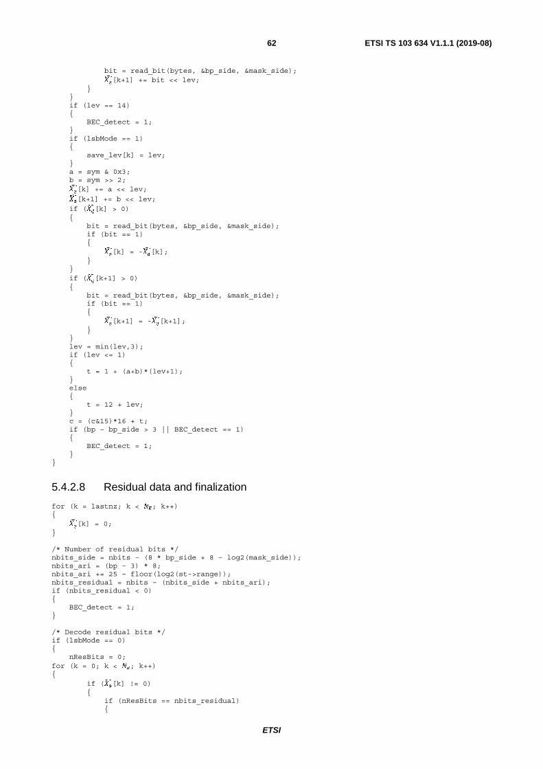
ETSI
ETSI TS 103 634 V1.1.1 (2019-08)62
bit = read_bit(bytes, &bp_side, &mask_side); ���[k+1] += bit << lev; } } if (lev == 14) { BEC_detect = 1; } if (lsbMode == 1) { save_lev[k] = lev; } a = sym & 0x3; b = sym >> 2; ���[k] += a << lev;
���[k+1] += b << lev;
if (���[k] > 0) { bit = read_bit(bytes, &bp_side, &mask_side); if (bit == 1) { ���[k] = -���[k]; } } if (���[k+1] > 0) { bit = read_bit(bytes, &bp_side, &mask_side); if (bit == 1) { ���[k+1] = -���[k+1]; } } lev = min(lev,3); if (lev <= 1) { t = 1 + (a+b)*(lev+1); } else { t = 12 + lev; } c = (c&15)*16 + t; if (bp – bp_side > 3 || BEC_detect == 1) { BEC_detect = 1; } }
5.4.2.8 Residual data and finalization
for (k = lastnz; k < ��; k++) { ���[k] = 0; } /* Number of residual bits */ nbits_side = nbits – (8 * bp_side + 8 – log2(mask_side)); nbits_ari = (bp – 3) * 8; nbits_ari += 25 – floor(log2(st->range)); nbits_residual = nbits – (nbits_side + nbits_ari); if (nbits_residual < 0) { BEC_detect = 1; } /* Decode residual bits */ if (lsbMode == 0) { nResBits = 0; for (k = 0; k < ��; k++) { if (���[k] != 0) { if (nResBits == nbits_residual) {
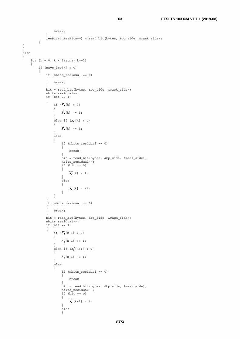
ETSI
ETSI TS 103 634 V1.1.1 (2019-08)63
break; } resBits[nResBits++] = read_bit(bytes, &bp_side, &mask_side); } } } else { for (k = 0; k < lastnz; k+=2) { if (save_lev[k] > 0) { if (nbits_residual == 0) { break; } bit = read_bit(bytes, &bp_side, &mask_side); nbits_residual--; if (bit == 1) { if (���[k] > 0) { ���[k] += 1; } else if (���[k] < 0) { ���[k] -= 1; } else { if (nbits_residual == 0) { break; } bit = read_bit(bytes, &bp_side, &mask_side); nbits_residual--; if (bit == 0) { ���[k] = 1; } else { ���[k] = -1; } } } if (nbits_residual == 0) { break; } bit = read_bit(bytes, &bp_side, &mask_side); nbits_residual--; if (bit == 1) { if (���[k+1] > 0) { ���[k+1] += 1; } else if (���[k+1] < 0) { ���[k+1] -= 1; } else { if (nbits_residual == 0) { break; } bit = read_bit(bytes, &bp_side, &mask_side); nbits_residual--; if (bit == 0) { ���[k+1] = 1; } else {
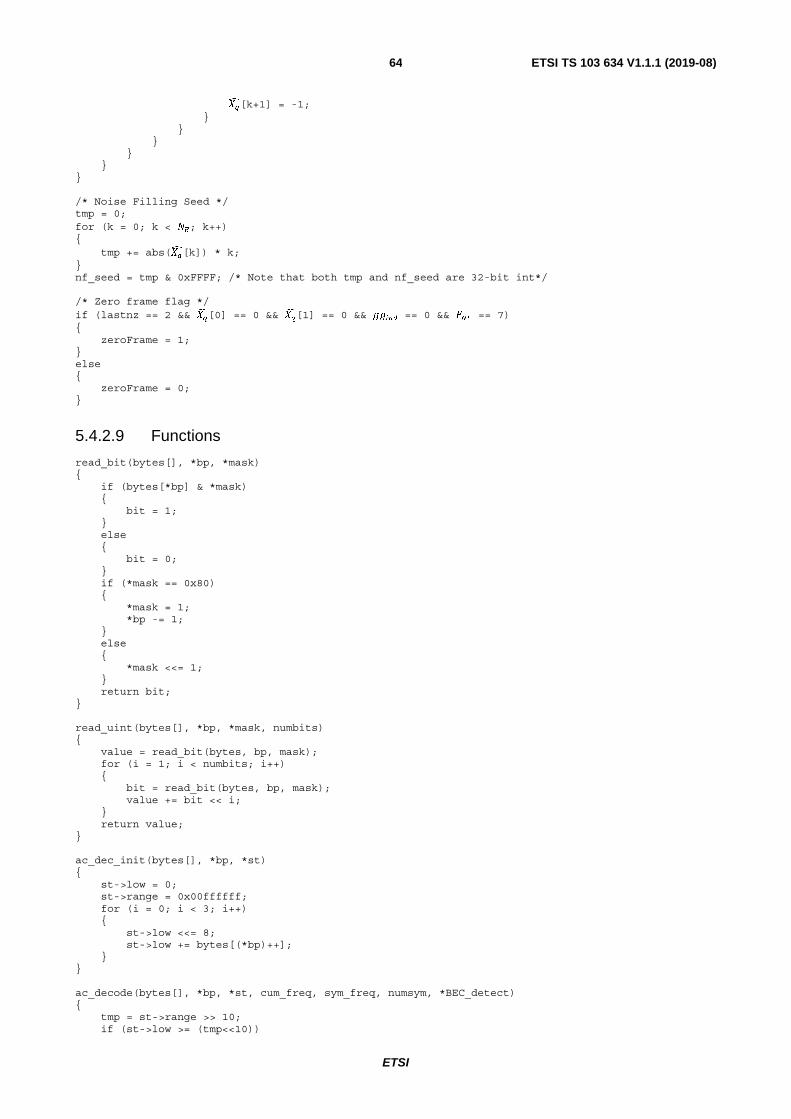
ETSI
ETSI TS 103 634 V1.1.1 (2019-08)64
���[k+1] = -1; } } } } } } /* Noise Filling Seed */ tmp = 0; for (k = 0; k < ��; k++) { tmp += abs(���[k]) * k; } nf_seed = tmp & 0xFFFF; /* Note that both tmp and nf_seed are 32-bit int*/ /* Zero frame flag */ if (lastnz == 2 && ���[0] == 0 && ���[1] == 0 && ����� == 0 && �� == 7) { zeroFrame = 1; } else { zeroFrame = 0; }
5.4.2.9 Functions
read_bit(bytes[], *bp, *mask) { if (bytes[*bp] & *mask) { bit = 1; } else { bit = 0; } if (*mask == 0x80) { *mask = 1; *bp -= 1; } else { *mask <<= 1; } return bit; } read_uint(bytes[], *bp, *mask, numbits) { value = read_bit(bytes, bp, mask); for (i = 1; i < numbits; i++) { bit = read_bit(bytes, bp, mask); value += bit << i; } return value; } ac_dec_init(bytes[], *bp, *st) { st->low = 0; st->range = 0x00ffffff; for (i = 0; i < 3; i++) { st->low <<= 8; st->low += bytes[(*bp)++]; } } ac_decode(bytes[], *bp, *st, cum_freq, sym_freq, numsym, *BEC_detect) { tmp = st->range >> 10; if (st->low >= (tmp<<10))
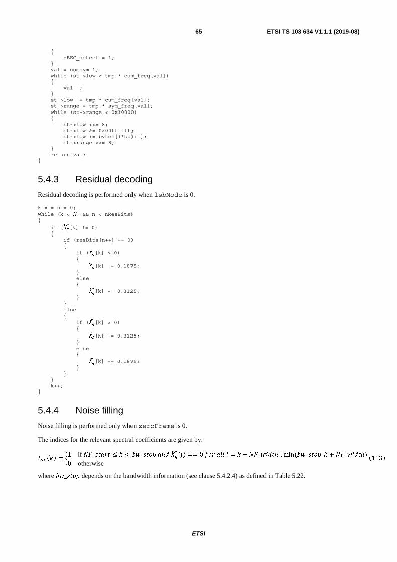
ETSI
ETSI TS 103 634 V1.1.1 (2019-08)65
{ *BEC_detect = 1; } val = numsym-1; while (st->low < tmp * cum_freq[val]) { val--; } st->low -= tmp * cum_freq[val]; st->range = tmp * sym_freq[val]; while (st->range < 0x10000) { st->low <<= 8; st->low &= 0x00ffffff; st->low += bytes[(*bp)++]; st->range <<= 8; } return val; }
5.4.3 Residual decoding
Residual decoding is performed only when lsbMode is 0.
k = = n = 0; while (k < �� && n < nResBits) { if (���[k] != 0) { if (resBits[n++] == 0) { if (���[k] > 0) { ���[k] -= 0.1875; } else { ���[k] -= 0.3125; } } else { if (���[k] > 0) { ���[k] += 0.3125; } else { ���[k] += 0.1875; } } } k++; }
5.4.4 Noise filling
Noise filling is performed only when zeroFrame is 0.
The indices for the relevant spectral coefficients are given by:
������ = !1 if ��_�� ≤ � < " _#$ ��� ��%��� == 0 �#� �&& � = � −��_ ��ℎ. . min�" _#$, � +��_ ��ℎ�0 otherwise
�113�
where " _#$ depends on the bandwidth information (see clause 5.4.2.4) as defined in Table 5.22.
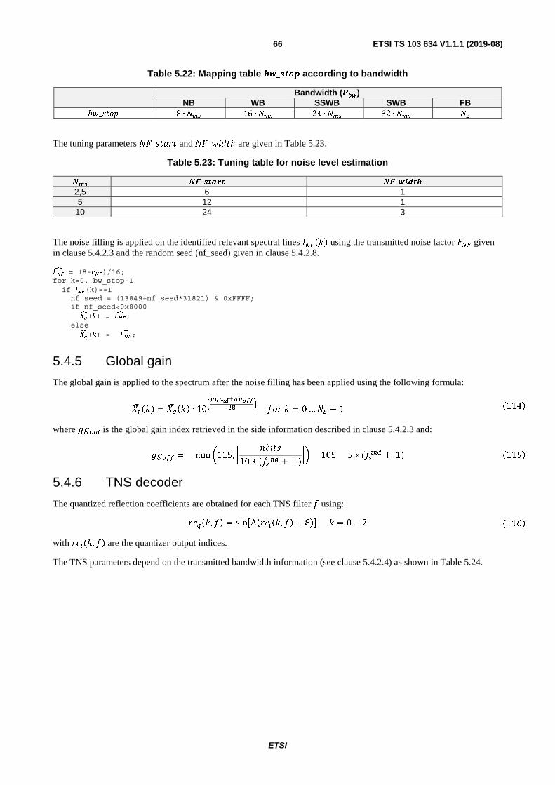
ETSI
ETSI TS 103 634 V1.1.1 (2019-08)66
Table 5.22: Mapping table ��_���� according to bandwidth
Bandwidth (���) NB WB SSWB SWB FB
��_���� 8 ∙ ��� 16 ∙ ��� 24 ∙ ��� 32 ∙ ��� ��
The tuning parameters ��_�� and ��_ ��ℎ are given in Table 5.23.
Table 5.23: Tuning table for noise level estimation
�� _�� �� _����� 2,5 6 1 5 12 1
10 24 3
The noise filling is applied on the identified relevant spectral lines ������ using the transmitted noise factor ��� given in clause 5.4.2.3 and the random seed (nf_seed) given in clause 5.4.2.8.
��� = (8-��)/16; for k=0..bw_stop-1 if ��(k)==1 nf_seed = (13849+nf_seed*31821) & 0xFFFF; if nf_seed<0x8000 ���(�) = ��� ; else ���(�) = −��� ;
5.4.5 Global gain
The global gain is applied to the spectrum after the noise filling has been applied using the following formula:
��%��� = ��%��� ∙ 10�������������� �
�#� � = 0 …� − 1 �114�
where ����� is the global gain index retrieved in the side information described in clause 5.4.2.3 and:
����� = − min '115, ( �"�10 ∗ (����� + 1)
)*− 105 − 5 ∗ (����� + 1) �115�
5.4.6 TNS decoder
The quantized reflection coefficients are obtained for each TNS filter � using:
�+���, �� = sin,Δ��+���, �� − 8�- � = 0 … 7 �116� with �+���, �� are the quantizer output indices.
The TNS parameters depend on the transmitted bandwidth information (see clause 5.4.2.4) as shown in Table 5.24.
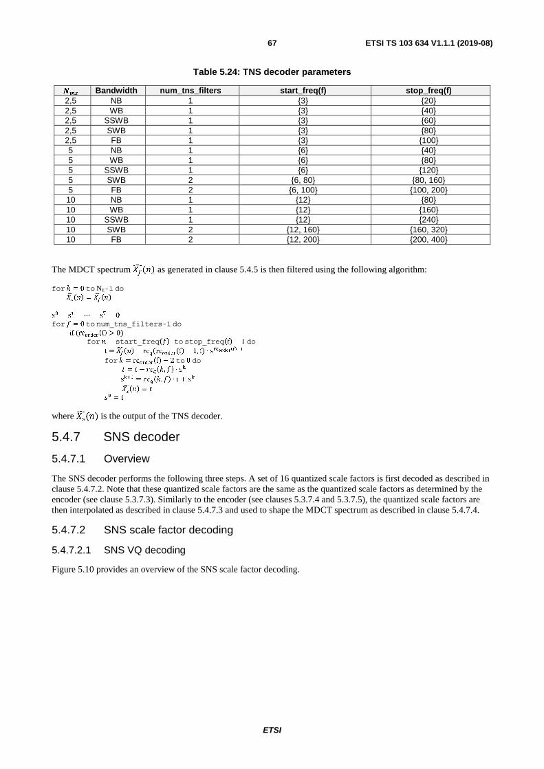
ETSI
ETSI TS 103 634 V1.1.1 (2019-08)67
Table 5.24: TNS decoder parameters
�� Bandwidth num_tns_filters start_freq(f) stop_freq(f) 2,5 NB 1 {3} {20} 2,5 WB 1 {3} {40} 2,5 SSWB 1 {3} {60} 2,5 SWB 1 {3} {80} 2,5 FB 1 {3} {100} 5 NB 1 {6} {40} 5 WB 1 {6} {80} 5 SSWB 1 {6} {120} 5 SWB 2 {6, 80} {80, 160} 5 FB 2 {6, 100} {100, 200} 10 NB 1 {12} {80} 10 WB 1 {12} {160} 10 SSWB 1 {12} {240} 10 SWB 2 {12, 160} {160, 320} 10 FB 2 {12, 200} {200, 400}
The MDCT spectrum ��%��� as generated in clause 5.4.5 is then filtered using the following algorithm:
for � = 0 to NE-1 do � ��� = ����� s� = s� = ⋯ = s� = 0 for � = 0 to num_tns_filters-1 do if (rc������f > 0)
for � = start_freq�� to stop_freq�f − 1 do
t = ����� − rc��rc������f − 1, f ∙ s������������
for � = rc�����f� − 2 to 0 do
� = � − ����,�� ∙ s�
s��� = ����,�� ∙ � + ��
��� = � �� = �
where ���(�) is the output of the TNS decoder.
5.4.7 SNS decoder
5.4.7.1 Overview
The SNS decoder performs the following three steps. A set of 16 quantized scale factors is first decoded as described in clause 5.4.7.2. Note that these quantized scale factors are the same as the quantized scale factors as determined by the encoder (see clause 5.3.7.3). Similarly to the encoder (see clauses 5.3.7.4 and 5.3.7.5), the quantized scale factors are then interpolated as described in clause 5.4.7.3 and used to shape the MDCT spectrum as described in clause 5.4.7.4.
5.4.7.2 SNS scale factor decoding
5.4.7.2.1 SNS VQ decoding
Figure 5.10 provides an overview of the SNS scale factor decoding.

ETSI
ETSI TS 103 634 V1.1.1 (2019-08)68
Figure 5.10: High level overview of Decoder SNS scale factor synthesis
5.4.7.2.2 Stage 1 SNS VQ decoding
The first stage parameters are decoded as follows:
ind_LF = read_uint(bytes, &bp_side, &mask_side, 5); /* stage1 LF */ ind_HF = read_uint(bytes, &bp_side, &mask_side, 5); /* stage1 HF */
The first stage indices ind_LF and ind_HF are converted into signal st1(n) according to equations �36� and (37) in clause 5.3.7.3.2.
5.4.7.2.3 Stage 2 SNS VQ decoding
5.4.7.2.3.1 Stage 2 SNS-VQ index demultiplexing
To efficiently use the available total bit space for the scale factor quantizer (38 bits), in combination with the fractional sized MPVQ-indices, the shape selection LSB, the second stage shape codewords and the adjustment gain least significant bit were jointly encoded as described in Table 5.14 and the subsequent paragraph in the encoder clause 5.3.7.3.4.
On the decoder/receiver side the reverse process takes place.
The second stage MSB submode bit, initial gain index and the Leading Sign index are first read from the decoded bitstream decoded as follows:
submodeMSB = read_bit(bytes, &bp_side, &mask_side); if( submodeMSB == 0 ){ Gind = read_uint(bytes, &bp_side, &mask_side, 1); } else { Gind = read_uint(bytes, &bp_side, &mask_side, 2); } LS_indA = read_bit(bytes, &bp_side, &mask_side); /* LS_indA 1 bit */
If submodeMSB equals 0, corresponding to one of the shapes (shape_j =0 or shape_j =1), the following demultiplexing procedure is followed:
/* 'regular'/'regular_lf' demultiplexing, establish if shape_j is 0 or 1 */ tmp = read_uint(bytes, &bp_side, &mask_side, 13) ; tmp |= (read_uint(bytes, &bp_side, &mask_side, 12)<<13) ; [ BEC_detect, submodeLSB, idxA, idxBorGainLSB ] = dec_split_st2VQ_CW(tmp, 4780008U>>1, 14 ); if( submodeLSB != 0 ) { Gind = (Gind<<1) + idxBorGainLSB; /* for regular_lf */ } else { idxB = idxBorGainLSB>>1; /* for regular */ LS_indB = idxBorGainLSB&0x1); }
with function dec_split_st2VQ_CW defined as:
[BEC_detect, submodeLSB, idxA, idxBorGainLSB ] =
dec_split_st2VQ_CW(cwRx, szA, szB ) {
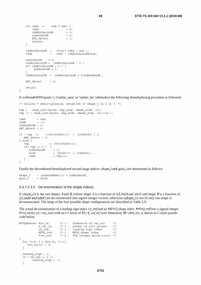
ETSI
ETSI TS 103 634 V1.1.1 (2019-08)69
if( cwRx >= szB * szA) { idxA = 0; idxBorGainLSB = 0; submodeLSB = 0; BEC_detect = 1; return; } idxBorGainLSB = floor( cwRx / szA ); idxA = cwRx – idxBorGainLSB*szA; submodeLSB = 0; idxBorGainLSB = idxBorGainLSB – 2 ; if( idxBorGainLSB < 0 ) { submodeLSB = 1; } idxBorGainLSB = idxBorGainLSB + 2*submodeLSB ; BEC_detect = 0; return; }
If submodeMSB equals 1, ('outlier_near' or 'outlier_far' submodes) the following demultiplexing procedure is followed:
/* outlier_* demultiplexing, establish if shape_j is 2 or 3 */ tmp = read_uint(bytes, &bp_side, &mask_side, 12); tmp |= ( read_uint(bytes, &bp_side, &mask_side, 12)<<12 ); idxA = tmp; idxB = -1; submodeLSB = 0; BEC_detect = 0; if ( tmp >= ((30316544U>>1) + 1549824U) ) { BEC_detect = 1; } else { tmp -= (30316544U>>1); if( tmp >= 0 ) { submodeLSB = 1; Gind = (Gind<<1) + (tmp&0x1); idxA = tmp>>1; } }
Finally the decombined/demultiplexed second stage indices shape_j and gain_i are determined as follows:
shape_j = (submodeMSB<<1) + submodeLSB; gain_i = Gind;
5.4.7.2.3.2 De-enumeration of the shape indices
If shape_j is 0, the two shapes A and B, (where shape A is a function of LS_indA and idxA, and shape B is a function of LS_indB and idxB) are de-enumerated into signed integer vectors, otherwise (shape_j is not 0) only one shape is de-enumerated. The setup of the four possible shape configurations are described in Table 5.9.
The actual de-enumeration of a leading sign index LS_ind and an MPVQ shape index MPVQ_ind into a signed integer PVQ vector y
(=vec_out) with an L1 norm of K (=k_val_in) over dimension N(=dim_in), is shown in C-style pseudo code below.
MPVQdeenum( dim_in, /* i : dimension of vec_out */ k_val_in, /* i : number of unit pulses */ LS_ind, /* i : leading sign index */ MPVQ_ind, /* i : MPVQ shape index */ *vec_out /* o : PVQ integer pulse train */ { for (i=0; i < dim_in; i++){ vec_out[i] = 0; } leading_sign = 1; if ( LS_ind != 0 ){ leading_sign = -1; }
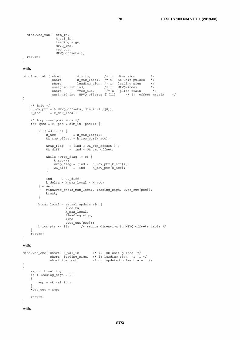
ETSI
ETSI TS 103 634 V1.1.1 (2019-08)70
mind2vec_tab ( dim_in, k_val_in, leading_sign, MPVQ_ind, vec_out, MPVQ_offsets ); return; }
with:
mind2vec_tab ( short dim_in, /* i: dimension */ short k_max_local, /* i: nb unit pulses */ short leading_sign, /* i: leading sign */ unsigned int ind, /* i: MPVQ-index */ short *vec_out, /* o: pulse train */ unsigned int MPVQ_offsets [][11] /* i: offset matrix */ ) { /* init */ h_row_ptr = &(MPVQ_offsets[(dim_in-1)][0]); k_acc = k_max_local; /* loop over positions */ for (pos = 0; pos < dim_in; pos++) { if (ind != 0) { k_acc = k_max_local;; UL_tmp_offset = h_row_ptr[k_acc]; wrap_flag = (ind < UL_tmp_offset ) ; UL_diff = ind - UL_tmp_offset; while (wrap_flag != 0) { k_acc--; wrap_flag = (ind < h_row_ptr[k_acc]); UL_diff = ind - h_row_ptr[k_acc]; } ind = UL_diff; k_delta = k_max_local - k_acc; } else { mind2vec_one(k_max_local, leading_sign, &vec_out[pos]); break; } k_max_local = setval_update_sign( k_delta, k_max_local, &leading_sign, &ind, &vec_out[pos]); h_row_ptr -= 11; /* reduce dimension in MPVQ_offsets table */ } return; }
with:
mind2vec_one( short k_val_in, /* i: nb unit pulses */ short leading_sign, /* i: leading sign -1, 1 */ short *vec_out /* o: updated pulse train */ ) { amp = k_val_in; if ( leading_sign < 0 ) { amp = -k_val_in ; } *vec_out = amp; return; }
with:
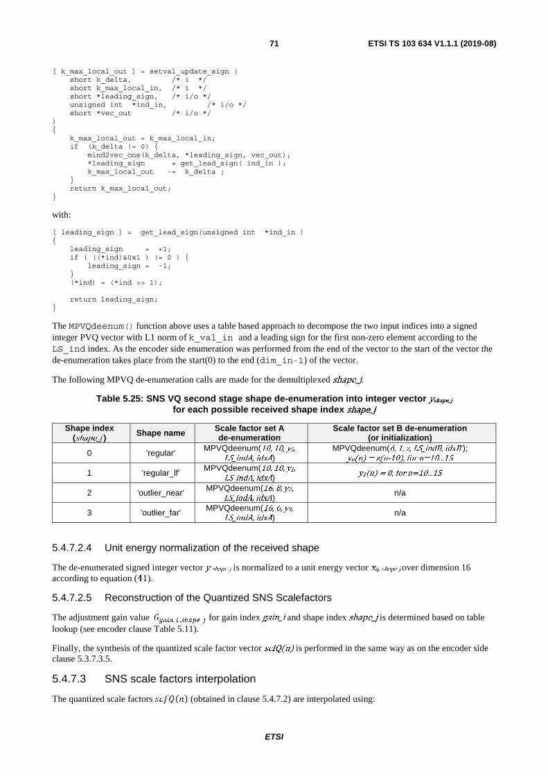
ETSI
ETSI TS 103 634 V1.1.1 (2019-08)71
[ k_max_local_out ] = setval_update_sign ( short k_delta, /* i */ short k_max_local_in, /* i */ short *leading_sign, /* i/o */ unsigned int *ind_in, /* i/o */ short *vec_out /* i/o */ ) { k_max_local_out = k_max_local_in; if (k_delta != 0) { mind2vec_one(k_delta, *leading_sign, vec_out); *leading_sign = get_lead_sign( ind_in ); k_max_local_out -= k_delta ; } return k_max_local_out; }
with:
[ leading_sign ] = get_lead_sign(unsigned int *ind_in ) { leading_sign = +1; if ( ((*ind)&0x1 ) != 0 ) { leading_sign = -1; } (*ind) = (*ind >> 1); return leading_sign; }
The MPVQdeenum() function above uses a table based approach to decompose the two input indices into a signed integer PVQ vector with L1 norm of k_val_in and a leading sign for the first non-zero element according to the LS_ind index. As the encoder side enumeration was performed from the end of the vector to the start of the vector the de-enumeration takes place from the start(0) to the end (dim_in-1) of the vector.
The following MPVQ de-enumeration calls are made for the demultiplexed shape_j.
Table 5.25: SNS VQ second stage shape de-enumeration into integer vector yshape_j for each possible received shape index shape_j
Shape index (shape_j ) Shape name Scale factor set A
de-enumeration Scale factor set B de-enumeration
(or initialization)
0 'regular' MPVQdeenum(10, 10, y0,
LS_indA, idxA) MPVQdeenum(6, 1, z, LS_indB, idxB );
yo(n) = z(n-10), for n=10...15
1 'regular_lf' MPVQdeenum(10, 10, y1,
LS_indA, idxA) y1(n) = 0, for n=10...15
2 'outlier_near' MPVQdeenum(16, 8, y2, LS_indA, idxA)
n/a
3 'outlier_far' MPVQdeenum(16, 6, y3, LS_indA, idxA)
n/a
5.4.7.2.4 Unit energy normalization of the received shape
The de-enumerated signed integer vector y shape_j is normalized to a unit energy vector xq, shape_j over dimension 16 according to equation (41).
5.4.7.2.5 Reconstruction of the Quantized SNS Scalefactors
The adjustment gain value �����_� ,�����_ for gain index gain_i and shape index shape_j is determined based on table lookup (see encoder clause Table 5.11).
Finally, the synthesis of the quantized scale factor vector scfQ(n) is performed in the same way as on the encoder side clause 5.3.7.3.5.
5.4.7.3 SNS scale factors interpolation
The quantized scale factors ������� (obtained in clause 5.4.7.2) are interpolated using:

ETSI
ETSI TS 103 634 V1.1.1 (2019-08)72
������0� = �����0�������1� = �����0�
������4� + 2� = ������� +1
8������� + 1� − �������� � � � = 0 … 14
������4� + 3� = ������� +3
8������� + 1� − �������� � � � = 0 … 14
������4� + 4� = ������� +5
8������� + 1� − �������� � � � = 0 … 14
������4� + 5� = ������� +7
8������� + 1� − �������� � � � = 0 … 14
������62� = �����15� +1
8������15� − �����14��
������63� = �����15� +3
8������15� − �����14��
�117�
In case, the codec is configured to operate on a number of bands � < 64, the number of scale factors need to be reduced using the following pseudo code:
If �� < 32 n4=round(abs(1-32/��)* ��) n2 = �� - n4 for i=0…n4-1
tmp(i) = �
�∑ �������(�)����������
for i=0…n2-1
tmp(n4-1+i) = �
�∑ �������(�)������������
����������
else if � < 64 n2 = 64 -�;
for i=0…n2-1
tmp(i) = �
�∑ �������(�)����������
for i=0… � tmp(n2-1+i) = �������(n2 − 1� ∗ 2 + �)
In case �� < 64, the the vector tmp is copied to �������. Finally, the scale factors are transformed back into linear domain using:
����� = 2������� � � � = 0. . .�� 118�
5.4.7.4 Spectral Shaping
The SNS scale factors ����� are applied on the TNS filtered MDCT frequency lines for each band separately as outlined in order to generate the shaped spectrum ��(�) as outlined by the following code:
for (b=0; b< ; b++) { for (k=���( ); k< ���( + 1); k++) {
��(�) = ����� ∙ ���� � } }
5.4.8 Low delay MDCT synthesis
The reconstructed spectrum ��(�) is transformed to the time domain by the following steps:
1) Generation of time domain aliasing buffer �̂�� �̂�� = � 2��
� ��(�) cos � ���
�� +1
2+
��
2� �� +
1
2������
���
� � � = 0 … 2�� − 1 119�
2) Windowing of time-aliased buffer

ETSI
ETSI TS 103 634 V1.1.1 (2019-08)73
�̂��� � �������2 1 �� ∙ �̂��� ��� � � 0 … 2� 1 �120�
3) Conduct overlap-add operation to get reconstructed time samples �����
����� � ������������ �̂�� � �� ��� � � 0 … � � 1 �121�
����� � �̂�� � �� ��� � � � � … � 1 �122�
������������ �̂�� � � � �� ��� � � 0 … � � 1 �123�
with ���_���_������ is initialized to 0 before decoding the first frame.
Please also consult clause 5.3.3 regarding any definition related to the MDCT operation.
5.4.9 Long term postfilter
5.4.9.1 Overview
The decoded signal after MDCT synthesis is postfiltered in the time-domain using an IIR filter whose parameters depend on the LTPF bitstream data "pitch_index" and "ltpf_active". As the filter coefficients are a pre-defined set, the result of the IIR filter is always stable. To avoid any discontinuity when the parameters change from one frame to the next, a transition mechanism is applied on the first quarter of the current frame.
For simplicity, audio samples of past frames are accessed by negative indexing, e.g. ��1� is the most recent sample of the signal � in the previous frame. Note that in practice, a buffer mechanism would have to be implemented.
The LTPF sharpens the harmonic structure of the signal by attenuating the quantization noise in the spectral valleys. An example of an LTPF frequency response for a speech signal is given in Figure 5.11.
Figure 5.11: Example of LTPF frequency response for a speech signal: the harmonic structure is sharpened by attenuation of the spectral valleys and quantization noise is perceptually optimized
5.4.9.2 Transition handling
The transition corresponds to the first ��
� samples of the current frame (� � 0 …
��
� 1).
Note that mem_ ltpf_active corresponds to the value of ltpf_active in the previous frame (it is initialized to zero before the first frame is processed), ����� is the filter input signal (i.e. the decoded signal after MDCT synthesis), �������� is the filter output signal, the filter parameters ���, � �, �� and � are given below, and ���
��� , � ����, ��
��� and ����.

ETSI
ETSI TS 103 634 V1.1.1 (2019-08)74
Five different cases are considered:
1) First case: ltpf_active = 0 and mem_ ltpf_active = 0
������� = ���� 124�
2) Second case: ltpf_active = 1 and mem_ ltpf_active = 0
������� ← ���� −���
4
� � �������� − ������
���
− � �����, ��� ����� �� − �� +!��
2− ������
���
" 125�
3) Third case: ltpf_active = 0 and mem_ ltpf_active = 1
������� ← ���� − #1 −���
4
$� � ����������� − ������
���
− � ��������, ������ ����� �� − ����� +!��
2− ������
���
" 126� with ������, ������, ����� and ������ are the filter parameters computed in the previous frame:
4) Fourth case: ltpf_active = 1 and mem_ltpf_active = 1 and �� = ����� and ��� = ������
������� ← ���� − � �������� − ������
���
+ � �����, ��� ����� �� − �� +!��
2− ������
���
127� 5) Fifth case: ltpf_active = 1 and mem_ltpf_active = 1 and (�� ≠ ����� or ��� ≠ ������)
����� ��� ← ���� − #1 −���
4
$� � ����������� − ������
���
− � ��������, ������ ����� � �� − ����� +!��
2− ������
���
" 128�
������� ← ����� ��� −���
4
� � ���������� �� − ������
���
− � �����, ��� ����� �� − �� +!��
2− ������
���
" 129�
5.4.9.3 Remaining of the frame
The remaining of the frame corresponds to the last ���
� samples of the current frame (� =
��
�… �� − 1).
Two different cases are considered:
1) First case: ltpf_active = 0
������� = ���� 130�
2) Second case: ltpf_active = 1
������� ← ���� − � �������� − ������
���
+ � �����, ��� ����� �� − �� +!��
2− ������
���
131�
with ���� is the filter input signal (i.e. the decoded signal after MDCT synthesis), ������� is the filter output signal and � = 0 … �� − 1.
The integer part �� and the fractional part ��� of the LTPF pitch-lag are computed as follows. First the pitch-lag at 12,8 kHz (see clause 5.3.10) is recovered using:
pitch_int =
⎩⎪⎨⎪⎧pitch_index − 283 if pitch_index ≥ 440
)pitch_index
2* − 63 if 440 > pitch_index ≥ 380
)pitch_index
4* + 32 if 380 > pitch_index
132�
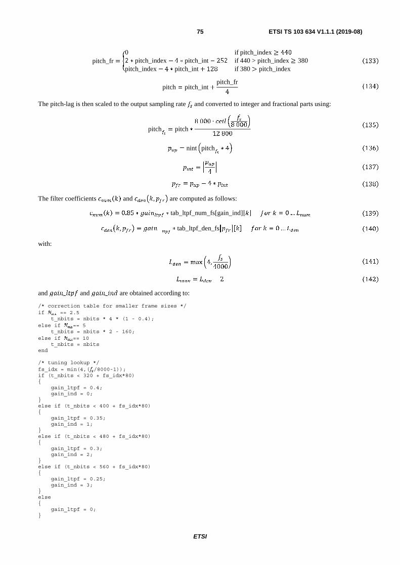
ETSI
ETSI TS 103 634 V1.1.1 (2019-08)75
pitch_fr = +0 if pitch_index ≥ 440
2 ∗ pitch_index − 4 ∗ pitch_int − 252 if 440 > pitch_index ≥ 380pitch_index − 4 ∗ pitch_int + 128 if 380 > pitch_index
133�
pitch = pitch_int +pitch_fr
4 134�
The pitch-lag is then scaled to the output sampling rate �� and converted to integer and fractional parts using:
pitch��
= pitch ∗8 000 ∙ �,�- � ��
8 000�
12 800
135�
��� = nint .pitch��
∗ 4/ 136�
�� = 0���4
1 137�
��� = ��� − 4 ∗ �� 138�
The filter coefficients ����� and �����, ��� are computed as follows:
����� = 0.85 ∗ 2����� ∗ tab_ltpf_num_fs[gain_ind]3�4 � � � = 0 … !�� 139�
�����, ��� = 2����
∗ tab_ltpf_den_fs5���63�4 � � � = 0 … !�� 140�
with:
!�� = max �4,��
4000� 141�
!�� = !�� − 2 142�
and 2��_-��� and 2��_��7 are obtained according to:
/* correction table for smaller frame sizes */ if �� == 2.5 t_nbits = nbits * 4 * (1 - 0.4); else if ��== 5 t_nbits = nbits * 2 - 160; else if ��== 10 t_nbits = nbits end /* tuning lookup */ fs_idx = min(4,(��/8000-1)); if (t_nbits < 320 + fs_idx*80) { gain_ltpf = 0.4; gain_ind = 0; } else if (t_nbits < 400 + fs_idx*80) { gain_ltpf = 0.35; gain_ind = 1; } else if (t_nbits < 480 + fs_idx*80) { gain_ltpf = 0.3; gain_ind = 2; } else if (t_nbits < 560 + fs_idx*80) { gain_ltpf = 0.25; gain_ind = 3; } else { gain_ltpf = 0; }

ETSI
ETSI TS 103 634 V1.1.1 (2019-08)76
The tables for tab_ltpf_num_fs�gain_ind���� and tab_ltpf_den_fs�������� are given in clause 5.9.5, Table 5.42.
5.4.10 Output signal scaling and rounding
The LTPF output signal ������ ��� for all samples with index � ∈ �0, �� � 1� is clipped to upper integer value range:
��������� ! 2 � 1, ��������� # 2 � 1�2, ��������� $ �2������ ���, %&ℎ()*+,( �143�
Afterwards, the signal ��������� is scaled to the proper range using:
����� �+�&���������� ∙ 2� ��� �144�
The output signal ����� is in the PCM integer format using , bits per sample.
5.5 Frame structure The frame structure of the codec consists of four parts, i.e.
• Side information containing static bits about the configuration of the frame data. This data block starts at the end of the frame and is read backwards. It includes information audio bandwidth, global gain, noise level, TNS activity, LTPF, SNS data, the index of the last non-zero spectral line and parts of the quantized spectrum. An exact bit stream definition can be found in clause 5.4.2.3.
• A dynamic data block which is arithmetically coded and contains TNS and fractional parts of the quantized spectrum. This block is read from the beginning of the frame towards the end. The decoding of this block is described in clause 5.4.2.4.
• A dynamic data block with signs and least significant bits part of the quantized spectrum. This block is read backwards from the end of the static side information bits. The decoding of this dynamic data block is described in clause 5.4.2.7.
• The residual data is located between the two dynamic data blocks and contains refinements of the quantized spectrum. It is read backwards starting immediately after the last encoded side information dynamic data block with spectrum signs and spectrum LSBs. The residual data is described according to clause 5.4.2.8.
Figure 5.12: Frame structure
5.6 Error concealment
5.6.1 General consideration
The purpose of the packet loss concealment (PLC) is to conceal the effect of unavailable or corrupted frame data for decoding. The overall composite PLC algorithm is described in clause 5.6.3 and when this composite algorithm shall be applied for the LC3, is described in clause 5.6.2.
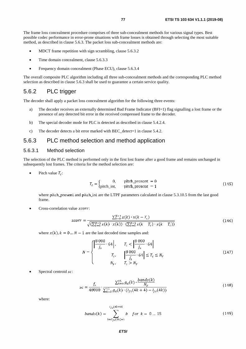
ETSI
ETSI TS 103 634 V1.1.1 (2019-08)77
The frame loss concealment procedure comprises of three sub-concealment methods for various signal types. Best possible codec performance in error-prone situations with frame losses is obtained through selecting the most suitable method, as described in clause 5.6.3. The packet loss sub-concealment methods are:
• MDCT frame repetition with sign scrambling, clause 5.6.3.2
• Time domain concealment, clause 5.6.3.3
• Frequency domain concealment (Phase ECU), clause 5.6.3.4
The overall composite PLC algorithm including all three sub-concealment methods and the corresponding PLC method selection as described in clause 5.6.3 shall be used to guarantee a certain service quality.
5.6.2 PLC trigger
The decoder shall apply a packet loss concealment algorithm for the following three events:
a) The decoder receives an externally determined Bad Frame Indicator (BFI=1) flag signalling a lost frame or the presence of any detected bit error in the received compressed frame to the decoder.
b) The special decoder mode for PLC is detected as described in clause 5.4.2.4.
c) The decoder detects a bit error marked with BEC_detect=1 in clause 5.4.2.
5.6.3 PLC method selection and method application
5.6.3.1 Method selection
The selection of the PLC method is performed only in the first lost frame after a good frame and remains unchanged in subsequently lost frames. The criteria for the method selection are:
• Pitch value ��:
�� = � 0, pitch_present = 0pitch_int, pitch_present = 1
�145�
where pitch_present and pitch_int are the LTPF parameters calculated in clause 5.3.10.5 from the last good frame.
• Cross-correlation value �����:
����� =∑ ��� ∙ �� − �����������∑ ��� ∙ ������
��� � ∙ �∑ �� − ��� ∙ �� − ��������� � �146�
where ���, = 0 … � − 1 are the last decoded time samples and:
� =
⎩⎪⎨⎪⎧�8 000�� ∙ 64� , �� < �8 000�� ∙ 64�
�� , �8 000�� ∙ 64� ≤ �� ≤ �� , �� > �
�147�
• Spectral centroid ��:
�� =��
48000∙
∑ �() ∙�����()�
�����∑ �()��
��� ∙ (����4 + 4� − ����4�)�148�
where:
������� = � � ��(����)
�� ��������
��� = 0 … 15 �149�
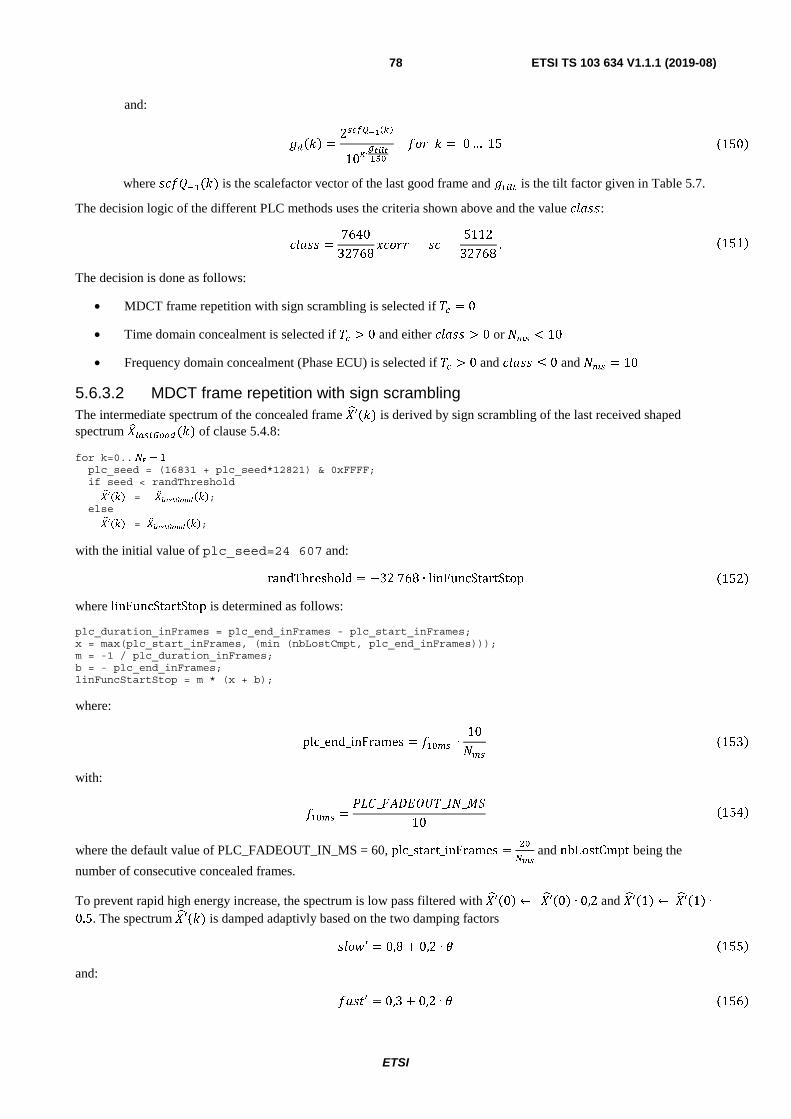
ETSI
ETSI TS 103 634 V1.1.1 (2019-08)78
and:
��� =2���������
10�∙��������
��� = 0 … 15 �150�
where ������() is the scalefactor vector of the last good frame and ����� is the tilt factor given in Table 5.7.
The decision logic of the different PLC methods uses the criteria shown above and the value �����:
����� =7640
32768����� − �� −
5112
32768. �151�
The decision is done as follows:
• MDCT frame repetition with sign scrambling is selected if �� = 0
• Time domain concealment is selected if �� > 0 and either ����� > 0 or ��� < 10
• Frequency domain concealment (Phase ECU) is selected if �� > 0 and ����� ≤ 0 and ��� = 10
5.6.3.2 MDCT frame repetition with sign scrambling The intermediate spectrum of the concealed frame �′� () is derived by sign scrambling of the last received shaped spectrum � �������() of clause 5.4.8:
for k=0.. �� − 1 plc_seed = (16831 + plc_seed*12821) & 0xFFFF; if seed < randThreshold
�′� (�) = −�������������; else
�′� (�) = �������������;
with the initial value of plc_seed=24 607 and:
randThreshold = −32 768 ∙ linFuncStartStop �152�
where linFuncStartStop is determined as follows:
plc_duration_inFrames = plc_end_inFrames - plc_start_inFrames; x = max(plc_start_inFrames, (min (nbLostCmpt, plc_end_inFrames))); m = -1 / plc_duration_inFrames; b = - plc_end_inFrames; linFuncStartStop = m * (x + b);
where:
plc_end_inFrames = ����� ∙10���
�153�
with:
����� =!"#_$%&'()�_��_*+
10�154�
where the default value of PLC_FADEOUT_IN_MS = 60, plc_start_inFrames =��
��� and nbLostCmpt being the
number of consecutive concealed frames.
To prevent rapid high energy increase, the spectrum is low pass filtered with �′� �0� ← �′� �0� ∙ 0,2 and �′� �1� ← �′� �1� ∙
0.5. The spectrum �′� () is damped adaptivly based on the two damping factors ���,′ = 0,8 + 0,2 ∙ - �155�
and: ���.′ = 0,3 + 0,2 ∙ - �156�

ETSI
ETSI TS 103 634 V1.1.1 (2019-08)79
where - is the stability factor computed as follows:
- = 1,25 −1
25�/�������� − ��������0���
���
�157�
where the stability factor - is truncated to 0 ≤ - ≤ 1, with larger values of - corresponding to more stable signals. This limits energy and spectral envelope fluctuations. If there are no two adjacent scale factor vectors present, - is set to 0,8. The two factors ���,′ and ���.′ are calculated if nbLostFrames = 1 and stay for consecutive lost frames. Based on these and the number of consecutive lost frames, the two damping factors ���,′′� and ���.′′� are calculated as follows:
���,′′� = ⎩⎨⎧ 0, 1� ��"��.#23._��� > ��������,′ ∙
����� − ��"��.#23._�������� − ��"��.#23._��� + 1, 4��4 1� ��"��.#23._��� > 2���,′, 4��4 �158�
and:
���.′′� = ⎩⎨⎧ 0, 1� ��"��.#23._��� > ��������.′ ∙
����� − ��"��.#23._�������� − ��"��.#23._��� + 1, 4��4 1� ��"��.#23._��� > 2���.′, 4��4 �159�
where:
��"��.#23._��� = ��"��.#23. +
10���− 1
10���
. �160�
Finally, the two damping factors ���,� and ���.� are calculated as follows:
���,� = 5����,′′�
, ��� ��� = 2,5����,′′�
, ��� ��� = 5���,′′� , �.ℎ4�,1�4 �161�
and:
���.� = 5����.′′�
, ��� ��� = 2,5����.′′�
, ��� ��� = 5���.′′� , �.ℎ4�,1�4 �162�
The corresponding cumulative attenuation factors cum_fading_slow� and cum_fading_fast� are calculated as follows:
cum_fading_slow� = cum_fading_slow��� ∙ ���,� �163�
and:
cum_fading_fast� = cum_fading_slow��� ∙ ���.� �164�
where cum_fading_slow��� and cum_fading_fast��� are the cumulative attenuation factors of the previous frame or 1 if nbLostFrames = 1.
Finally, the damping is processed as follows:
ad_ThreshFac_start = 10; ad_ThreshFac_end = 1.2; ad_threshFac = (ad_ThreshFac_start - ad_ThreshFac_end) * linFuncStartStop + ad_ThreshFac_end;
frame_energy = mean(��′(�)(0.. �� − 1).^2); energThreshold = ad_threshFac * frame_energy;
for k=0.. �� − 1
if (��′(�)^2) < energThreshold m = cum_fading_slow; n = 0; else
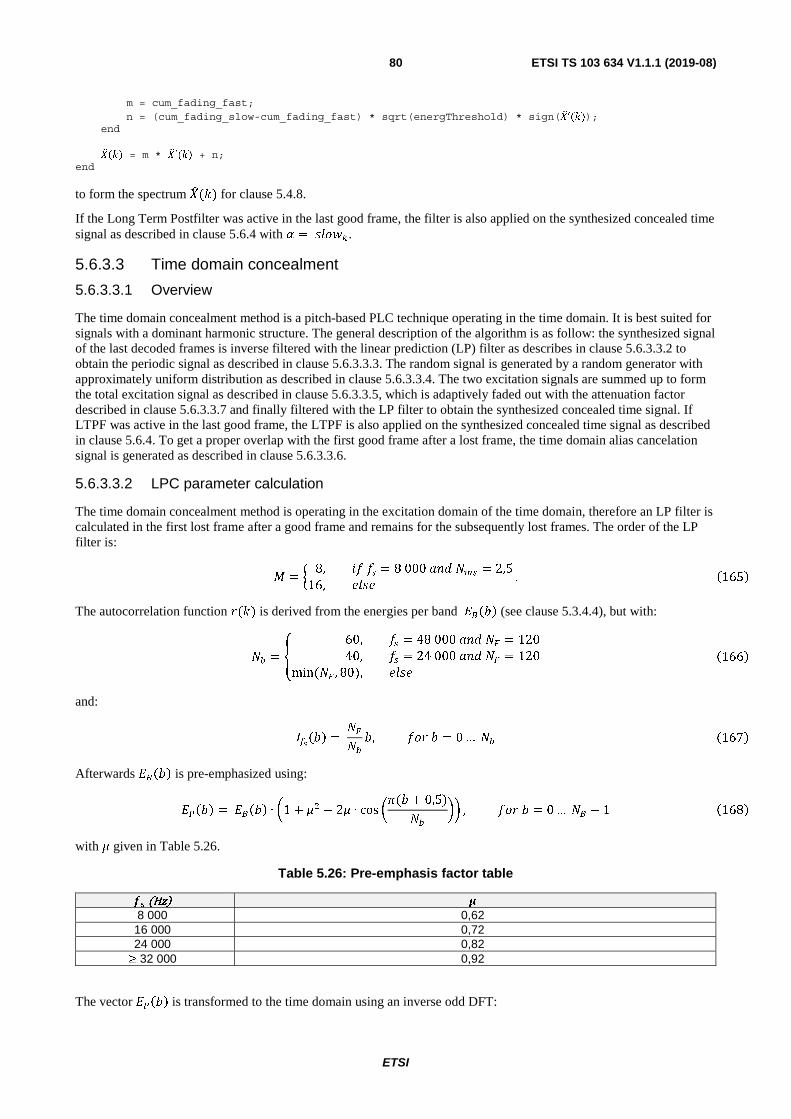
ETSI
ETSI TS 103 634 V1.1.1 (2019-08)80
m = cum_fading_fast; n = (cum_fading_slow-cum_fading_fast) * sqrt(energThreshold) * sign(��′(�)); end ��(�) = m * ��′(�) + n; end
to form the spectrum � () for clause 5.4.8.
If the Long Term Postfilter was active in the last good frame, the filter is also applied on the synthesized concealed time signal as described in clause 5.6.4 with 6 = ���,�.
5.6.3.3 Time domain concealment
5.6.3.3.1 Overview
The time domain concealment method is a pitch-based PLC technique operating in the time domain. It is best suited for signals with a dominant harmonic structure. The general description of the algorithm is as follow: the synthesized signal of the last decoded frames is inverse filtered with the linear prediction (LP) filter as describes in clause 5.6.3.3.2 to obtain the periodic signal as described in clause 5.6.3.3.3. The random signal is generated by a random generator with approximately uniform distribution as described in clause 5.6.3.3.4. The two excitation signals are summed up to form the total excitation signal as described in clause 5.6.3.3.5, which is adaptively faded out with the attenuation factor described in clause 5.6.3.3.7 and finally filtered with the LP filter to obtain the synthesized concealed time signal. If LTPF was active in the last good frame, the LTPF is also applied on the synthesized concealed time signal as described in clause 5.6.4. To get a proper overlap with the first good frame after a lost frame, the time domain alias cancelation signal is generated as described in clause 5.6.3.3.6.
5.6.3.3.2 LPC parameter calculation
The time domain concealment method is operating in the excitation domain of the time domain, therefore an LP filter is calculated in the first lost frame after a good frame and remains for the subsequently lost frames. The order of the LP filter is:
* = � 8, 1� �� = 8 000 ��� ��� = 2,5
16, 4��4 . �165�
The autocorrelation function �() is derived from the energies per band '���� (see clause 5.3.4.4), but with:
�� = 7 60, �� = 48 000 ��� � = 120
40, �� = 24 000 ��� � = 120
min (� , 80), 4��4 �166�
and:
������ = ���
�, ��� � = 0 … �� �167�
Afterwards '���� is pre-emphasized using:
'���� = '���� ∙ 81 + 9� − 29 ∙ cos 8:(� + 0,5)��
;; , ��� � = 0 … �� − 1 �168�
with 9 given in Table 5.26.
Table 5.26: Pre-emphasis factor table
�� (Hz) � 8 000 0,62 16 000 0,72 24 000 0,82
≥ 32 000 0,92
The vector ����� is transformed to the time domain using an inverse odd DFT:
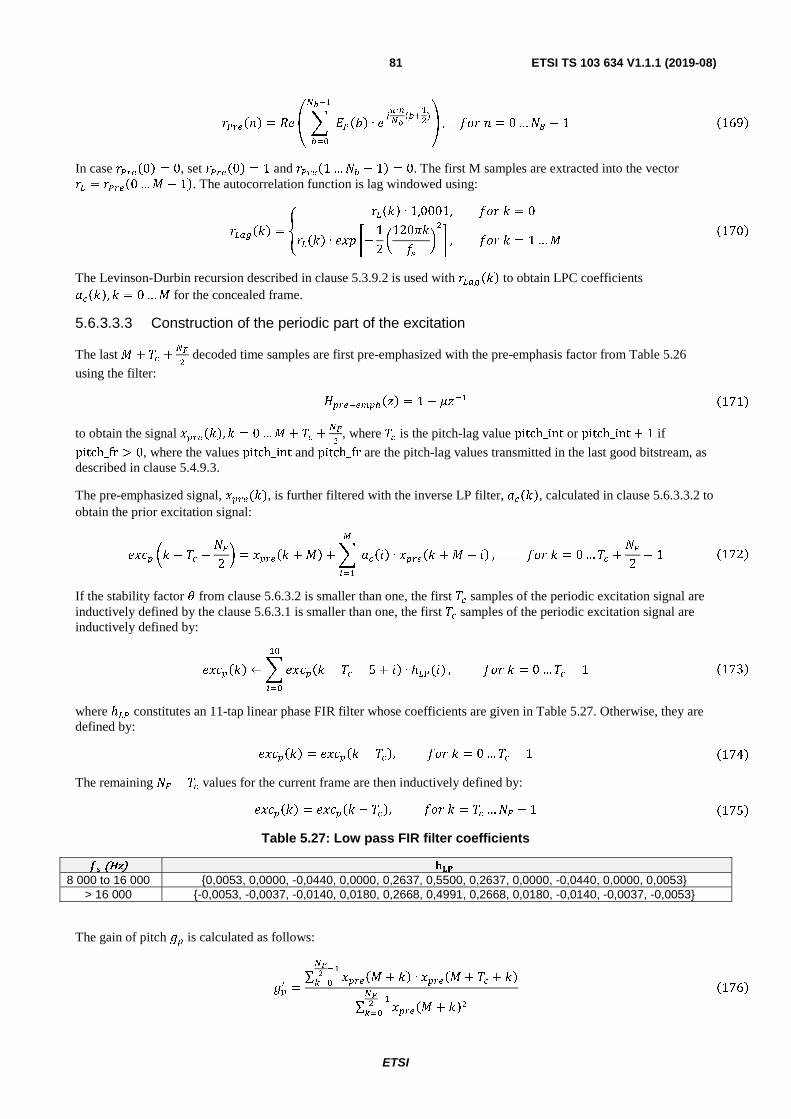
ETSI
ETSI TS 103 634 V1.1.1 (2019-08)81
������� = �� ����� ∙ ���∙���
(�
�)
���
� �
� , � � � = 0 …�� − 1 �169� In case �����0� = 0, set �����0� = 1 and �����1 …�� − 1� = 0. The first M samples are extracted into the vector �� = �����0 …� − 1�. The autocorrelation function is lag windowed using:
������� = � ����� ∙ 1,0001, � � � = 0����� ∙ ��� �− 1
2�120���� ��� , � � � = 1 …� �170�
The Levinson-Durbin recursion described in clause 5.3.9.2 is used with ������� to obtain LPC coefficients �����, � = 0 …� for the concealed frame.
5.6.3.3.3 Construction of the periodic part of the excitation
The last � + �� +��
� decoded time samples are first pre-emphasized with the pre-emphasis factor from Table 5.26
using the filter: ������������ = 1 − ��� �171� to obtain the signal �������, � = 0 …� + �� +
��
�, where �� is the pitch-lag value pitch_int or pitch_int + 1 if
pitch_fr > 0, where the values pitch_int and pitch_fr are the pitch-lag values transmitted in the last good bitstream, as described in clause 5.4.9.3.
The pre-emphasized signal, ����(�), is further filtered with the inverse LP filter, �����, calculated in clause 5.6.3.3.2 to obtain the prior excitation signal:
���� �� − �� −��2� = ������ + �� + ����� ∙ ������ + � − ���
�
, � � � = 0 … �� +��2
− 1 �172� If the stability factor from clause 5.6.3.2 is smaller than one, the first �� samples of the periodic excitation signal are inductively defined by the clause 5.6.3.1 is smaller than one, the first �� samples of the periodic excitation signal are inductively defined by:
������� ← ������ − �� − 5 + �� ∙ ℎ��(�)�
� �
, � � � = 0 …�� − 1 �173�
where ℎ�� constitutes an 11-tap linear phase FIR filter whose coefficients are given in Table 5.27. Otherwise, they are defined by: ������� = ������ − ���, � � � = 0 …�� − 1 �174� The remaining �� − �� values for the current frame are then inductively defined by: ������� = ������ − ���, � � � = �� …�� − 1 �175�
Table 5.27: Low pass FIR filter coefficients
�� (Hz) ��� 8 000 to 16 000 {0,0053, 0,0000, -0,0440, 0,0000, 0,2637, 0,5500, 0,2637, 0,0000, -0,0440, 0,0000, 0,0053}
> 16 000 {-0,0053, -0,0037, -0,0140, 0,0180, 0,2668, 0,4991, 0,2668, 0,0180, -0,0140, -0,0037, -0,0053}
The gain of pitch !� is calculated as follows:
!�� =∑ ������ + �� ∙ ������ + �� + ����
��
� � ∑ ������ + �������
� �
�176�
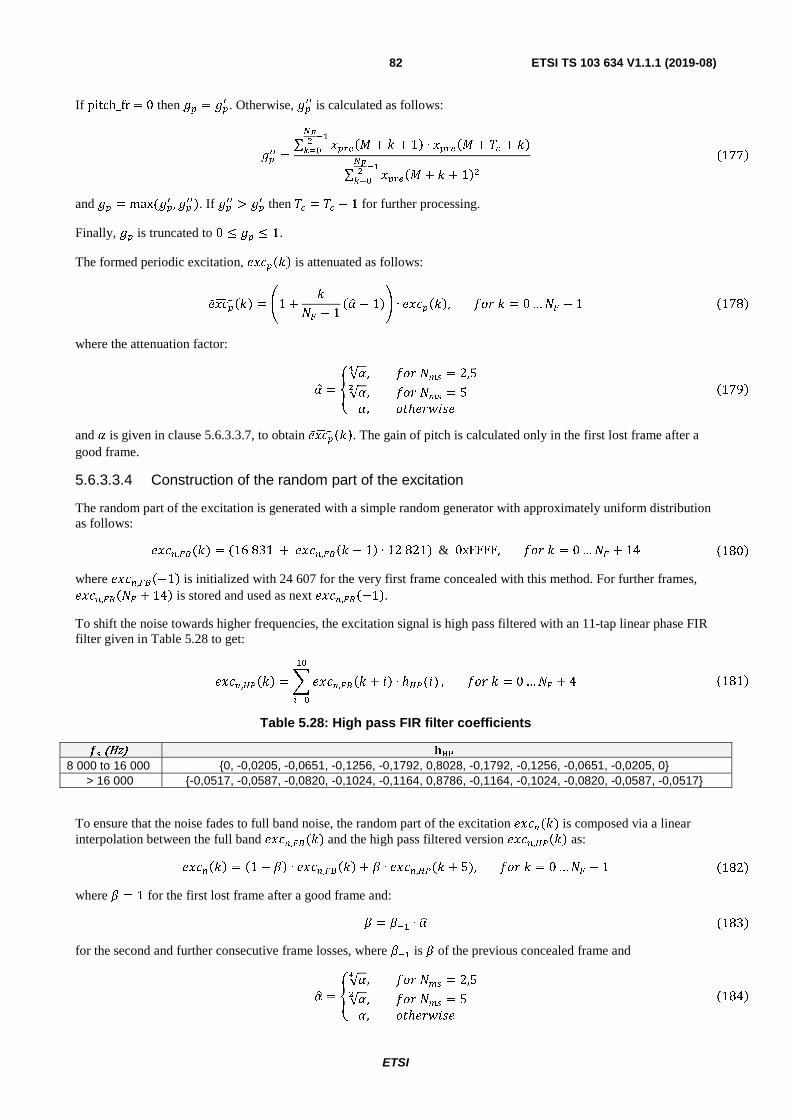
ETSI
ETSI TS 103 634 V1.1.1 (2019-08)82
If pitch_fr = 0 then !� = !�� . Otherwise, !��� is calculated as follows:
!��� =∑ ������ + � + 1� ∙ ������ + �� + ����
��
� � ∑ ������ + � + 1������
� �
�177� and !� = max (!�� ,!���). If !��� > !�� then �� = �� − 1 for further processing.
Finally, !� is truncated to 0 ≤ !� ≤ 1.
The formed periodic excitation, ������� is attenuated as follows:
����#��� = $1 +��� − 1
�%& − 1�' ∙ �������, � � � = 0 …�� − 1 �178� where the attenuation factor:
%& = �√%�, � � ��� = 2,5√%�, � � ��� = 5%, )ℎ��*�+� �179�
and % is given in clause 5.6.3.3.7, to obtain ����#���. The gain of pitch is calculated only in the first lost frame after a good frame.
5.6.3.3.4 Construction of the random part of the excitation
The random part of the excitation is generated with a simple random generator with approximately uniform distribution as follows: ����,��(�) = (16 831 + ����,���� − 1� ∙ 12 821) & 0xFFFF, � � � = 0 …�� + 14 �180� where ����,���−1� is initialized with 24 607 for the very first frame concealed with this method. For further frames, ����,����� + 14� is stored and used as next ����,���−1�. To shift the noise towards higher frequencies, the excitation signal is high pass filtered with an 11-tap linear phase FIR filter given in Table 5.28 to get:
����,����� = ����,���� + �� ∙ ℎ��(�)�
� �
, � � � = 0 …�� + 4 �181� Table 5.28: High pass FIR filter coefficients
�� (Hz) ��� 8 000 to 16 000 {0, -0,0205, -0,0651, -0,1256, -0,1792, 0,8028, -0,1792, -0,1256, -0,0651, -0,0205, 0}
> 16 000 {-0,0517, -0,0587, -0,0820, -0,1024, -0,1164, 0,8786, -0,1164, -0,1024, -0,0820, -0,0587, -0,0517}
To ensure that the noise fades to full band noise, the random part of the excitation ����(�) is composed via a linear interpolation between the full band ����,��(�) and the high pass filtered version ����,����� as: ������� = �1 − ,� ∙ ����,����� + , ∙ ����,��(� + 5), � � � = 0 …�� − 1 �182� where , = 1 for the first lost frame after a good frame and: , = ,� ∙ %& �183� for the second and further consecutive frame losses, where ,� is , of the previous concealed frame and
%& = �√%�, � � ��� = 2,5√%�, � � ��� = 5%, )ℎ��*�+� �184�

ETSI
ETSI TS 103 634 V1.1.1 (2019-08)83
The fading speed is dependent on the attenuation factor % calculated in clause 5.6.3.3.7. For adjusting the noise level, the gain of noise, !�� , is calculated as:
!�� =-∑ .���� /� −
��20 − !�1 ∙ ���� /� − �� −
��202���
��
� � ��/2
�185� where:
!�1 = 34!�� , � � ��� = 2,54!�� , � � ��� = 5!�, )ℎ��*�+� �186� and !� is the gain of pitch calculated in clause 5.6.3.3.3. To prevent high energy increase at �� = 8 000 ��, !�� is controlled by:
!�� ←
⎩⎪⎨⎪⎧-∑ .���� /� −
��202���
��
� � ��/2 , �� !�� >
-∑ .���� /� −��202���
��
� � ��/2 !�� , �9+��187�
If �� = pitch_int after clause 5.6.3.3.3, then !� = !�� . Otherwise, a second gain of noise, !���, is calculated as done in equation (185) and equation (187), but with �� = pitch_int. Following, !� = min (!�� ,!���).
The composed random excitation ������� is attenuated as follows:
����#��� = 3 !� ∙ �� ∙ �������, � � � = 0 … 4
$1 +� − 5�� − 1
�%& − 1�' ∙ !� ∙ �� ∙ �������, � � � = 5 …�� − 1�188�
where the normalization factor �� is:
�� = :1,1 − 0,75!�; ∙ 1<������� ∙ ��������� , � � � = 0 …�� − 1 �189�
to obtain ����#���. The noise gain, !�, is calculated only in the first lost frame after a good frame and is stored as !�,���� = !� ∙ % for the next consecutive frame loss, where !�,���� is the gain of noise of the next consecutive frame loss.
5.6.3.3.5 Construction of the total excitation, synthesis and post-processing
The random excitation, ����#���, is added to the periodic excitation, ����#���, to form the total excitation signal �������. The synthesized signal +=�)ℎ��� for the concealed frame is obtained by filtering the total excitation with the LP filter, �����, from clause 5.6.3.3.2 and post-processed with the de-emphasis filter, which is the inverse filter from equation (171).
If ��> +)?@�)_9 � = ���� and ��> +)?@�)_9 �� < ��> +)?@�)_9 �, with ��> +)?@�)_9 � from equation (160), ��> +)?@�)_9 �� is ��> +)?@�)_9 � from the previous frame and ���� from equation (154), then +=�)ℎ��� is faded out to zero as follows:
+=�)ℎ��� ← �1 −���� ∙ +=�)ℎ���, � � � = 0 …�� − 1 �190�
For further frame losses the signal and % is set to zero.
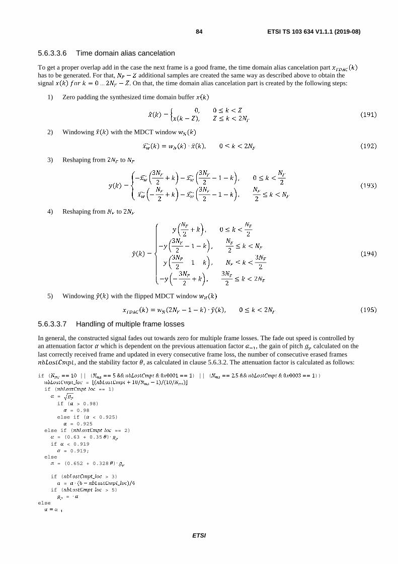
ETSI
ETSI TS 103 634 V1.1.1 (2019-08)84
5.6.3.3.6 Time domain alias cancelation
To get a proper overlap add in the case the next frame is a good frame, the time domain alias cancelation part � !"#��� has to be generated. For that, �� − A additional samples are created the same way as described above to obtain the signal ���� � � � = 0 … 2�� − A. On that, the time domain alias cancelation part is created by the following steps:
1) Zero padding the synthesized time domain buffer ���� �&��� = B 0, 0 ≤ � < A��� − A�, A ≤ � < 2�� �191�
2) Windowing �&��� with the MDCT window *�(�) �$1��� = *���� ∙ �&���, 0 ≤ � < 2�� �192� 3) Reshaping from 2�� to ��
=��� = 3−�$1 �3��2
+ �� − �$1 �3��2
− 1 − �� , 0 ≤ � <��2�$1 �−
��2
+ �� − �$1 �3��2
− 1 − �� ,��2
≤ � < �� �193� 4) Reshaping from �� to 2��
=&��� =
⎩⎪⎪⎨⎪⎪⎧ = ���
2+ �� , 0 ≤ � <
��2
−= �3��2
− 1 − �� ,��2
≤ � < ��−= �3��
2− 1 − �� , �� ≤ � <
3��2
−= �−3��
2+ �� ,
3��2
≤ � < 2���194�
5) Windowing =&��� with the flipped MDCT window *�(�) � !"#��� = *��2�� − 1 − �� ∙ =&���, 0 ≤ � < 2�� �195� 5.6.3.3.7 Handling of multiple frame losses
In general, the constructed signal fades out towards zero for multiple frame losses. The fade out speed is controlled by an attenuation factor % which is dependent on the previous attenuation factor %�, the gain of pitch !� calculated on the last correctly received frame and updated in every consecutive frame loss, the number of consecutive erased frames ��> +)?@�), and the stability factor , as calculated in clause 5.6.3.2. The attenuation factor is calculated as follows:
if (���
== 10 || (��� == 5 && ��������� & 00001 == 1) || (��� == 2.5 && ��������� & 00003 == 1)) ���������_�� = ⌊(��������� + 10/��� − 1)/(10/���)⌋ if (���������_�� == 1) � = ��� if (� > 0.98) � = 0.98 else if (� < 0.925) � = 0.925 else if (���������_�� == 2) � = (0.63 + 0.35 �)∙ �� if � < 0.919 � = 0.919; else � = (0.652 + 0.328 �)∙ �� if (���������_�� > 3) � = � ∙ (6 − ���������_�� )/4 if (���������_�� > 5) �� = ∙ � else � = ���
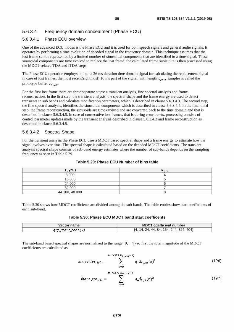
ETSI
ETSI TS 103 634 V1.1.1 (2019-08)85
5.6.3.4 Frequency domain concealment (Phase ECU)
5.6.3.4.1 Phase ECU overview
One of the advanced ECU modes is the Phase ECU and it is used for both speech signals and general audio signals. It operates by performing a time evolution of decoded signal in the frequency domain. This technique assumes that the lost frame can be represented by a limited number of sinusoidal components that are identified in a time signal. These sinusoidal components are time evolved to replace the lost frame, the calculated frame substitute is then processed using the MDCT-related TDA and ITDA steps.
The Phase ECU operation employs in total a 26 ms duration time domain signal for calculating the replacement signal in case of lost frames, the most recent(rightmost) 16 ms part of the signal, with length ����� samples is called the prototype buffer ������. For the first lost frame there are three separate steps: a transient analysis, fine spectral analysis and frame reconstruction. In the first step, the transient analysis, the spectral shape and the frame energy are used to detect transients in sub bands and calculate modification parameters, which is described in clause 5.6.3.4.3. The second step, the fine spectral analysis, identifies the sinusoidal components which is described in clause 5.6.3.4.4. In the final third step, the frame reconstruction, the sinusoids are time evolved and are converted back to the time domain and that is described in clause 5.6.3.4.5. In case of consecutive lost frames, that is during error bursts, processing consists of control parameter updates made by the transient analysis described in clause 5.6.3.4.3 and frame reconstruction as described in clause 5.6.3.4.5.
5.6.3.4.2 Spectral Shape
For the transient analysis the Phase ECU uses a MDCT based spectral shape and a frame energy to estimate how the signal evolves over time. The spectral shape is calculated based on the decoded MDCT coefficients. The transient analysis spectral shape consists of sub-band energy estimates where the number of sub-bands depends on the sampling frequency as seen in Table 5.29.
Table 5.29: Phase ECU Number of bins table
�� (Hz) ���� 8 000 4 16 000 5 24 000 6 32 000 7
44 100, 48 000 8
Table 5.30 shows how MDCT coefficients are divided among the sub-bands. The table entries show start coefficients of each sub-band.
Table 5.30: Phase ECU MDCT band start coefficents
Vector name MDCT coefficient number ���_�����_��( ) {4, 14, 24, 44, 84, 164, 244, 324, 404}
The sub-band based spectral shapes are normalized to the range [0, … 1) so first the total magnitude of the MDCT coefficients are calculated as:
�ℎ���_������� = � �_������(�)�
� (� , �������)
���
�196� �ℎ���_������ = � �_�����(�)�
� (� , �������)
���
�197�
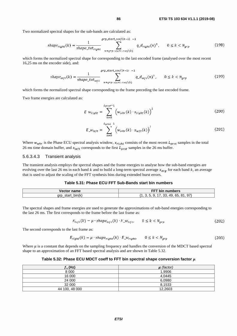
ETSI
ETSI TS 103 634 V1.1.1 (2019-08)86
Two normalized spectral shapes for the sub-bands are calculated as:
�ℎ��������� � =1�ℎ���_������� � �_������(�)�
���_�����_��������� ��
�����_�����_����(�)
, 0 ≤ < ���� �198� which forms the normalized spectral shape for corresponding to the last encoded frame (analysed over the most recent 16,25 ms on the encoder side), and:
�ℎ�������� � =1�ℎ���_������ � �_�����(�)�
���_�����_��������� ��
�����_�����_����(�)
, 0 ≤ < ���� �199� which forms the normalized spectral shape corresponding to the frame preceding the last encoded frame.
Two frame energies are calculated as:
�_������ = � ������ � ∙ ������� ����������
���
�200� �_����� = � ������ � ∙ ������ ���
�������
���
�201� Where ���� is the Phase ECU spectral analysis window, ������ consists of the most recent ����� samples in the total 26 ms time domain buffer, and ����� corresponds to the first ����� samples in the 26 ms buffer.
5.6.3.4.3 Transient analysis
The transient analysis employs the spectral shapes and the frame energies to analyse how the sub-band energies are evolving over the last 26 ms in each band and to build a long-term spectral average �� � for each band , an average that is used to adjust the scaling of the FFT synthesis bins during extended burst errors.
Table 5.31: Phase ECU FFT Sub-Bands start bin numbers
Vector name FFT bin numbers grp_start_bin(k) {1, 3, 5, 9, 17, 33, 49, 65, 81, 97}
The spectral shapes and frame energies are used to generate the approximations of sub-band energies corresponding to the last 26 ms. The first corresponds to the frame before the last frame as:
�����( ) = � ∙ �ℎ�������� � ∙ �_����� , 0 ≤ < ���� �202� The second corresponds to the last frame as:
������( ) = � ∙ �ℎ��������� � ∙ �_������ , 0 ≤ < ���� �203� Where � is a constant that depends on the sampling frequency and handles the conversion of the MDCT based spectral shape to an approximation of an FFT based spectral analysis and are shown in Table 5.32.
Table 5.32: Phase ECU MDCT coeff to FFT bin spectral shape conversion factor �
�� (Hz) � (factor) 8 000 1,9906 16 000 4,0445 24 000 6,0980 32 000 8,1533
44 100, 48 000 12,2603

ETSI
ETSI TS 103 634 V1.1.1 (2019-08)87
These are used to calculate the ratio of energies for the two positions as:
�����( ) =������( )�����( )
, 0 ≤ < ���� �204� This forms the basis of a frequency selective transient detection for each frequency band . The gain in compared with an upper and lower threshold that represent onset and offset detection respectively. If ������ � > 10 or ������ � < 0,1 is fulfilled the band contains a transient and ������ � is set to 1. The gains �!��� � are set to 1. If a band has a transient, the gain �!��� � is updated to:
�!��( ) = min �1,������� �� , 0 ≤ < ���� �205� The gains �!��� � for the first lost frame are saved into �′!��� �. To better handle burst conditions, magnitude and phase modification factors are updated. The first part in the magnitude modification is a low-resolution spectral shape, and is calculated according to the following:
������( ) = �1
2∙
������ � + ������( )���_�����_ !�� + 1� − ���_�����_ !�( ), 0 ≤ < ���� �206�
Here ������( ) now forms a low-resolution bin amplitude estimate in band . It is used for a generating a spectrally shaped additive noise signal to which the substitution signal is pulled towards in case of burst frame losses.
The second part in the magnitude modification is the adjustment of the gain �!��( ) which is updated band wise according to:
�!��( ) = �′!��( ) ∙ 10�"��
��# , 0 ≤ < ���� �207� where:
"��� = 0,30103���� = 3���� = 2�208�
# �!�� = 0, ����� ≤ ����
���� = ������ − ����� ∙ "��� , ���� < ����� ≤ �������� = ���� ∙ "��� + ������ − ����� ∙ 6,0206, ����� > ���� + ���� + ���� �209� Here ����� is the number of consecutive lost frames. If ����� > 5 then $!$�� = $!$�� ∙ 0,5.
The attenuation factors %( ) and $( ) are updated as:
%� � = �!��( )$� � = $!$�� ∙ �1 − %�( ) , 0 ≤ < ���� �210�
Through variable %( ) the concealment method is modified by selectively adjusting the magnitude of the substitution frame spectrum base on the frequency domain transient detector status �����( ).
The scaling factor $( ) is used to scale the spectrally shaped additive noise signal such that, except for the incorporated gradual muting behaviour through factor $!$��, it compensates for the energy loss caused by the attenuation with factor %( ).
For = 5, $( ) is further adjusted as $� � = $( ) ∙ 0,5 and for > 6 then $� � = $( ) ∙ 0,1. This superimposes a low-pass characteristic on the additive noise signal, which avoids unpleasant high frequency noise in the substitution signals.
5.6.3.4.4 Fine Spectral analysis
For the first lost frame the prototype frame buffer is used for a fine high-resolution spectral analysis:
&%( ) = FFT ������� ∙ ���������� , 0 ≤ � < ����� , 0 ≤ ≤ �%%& �211�
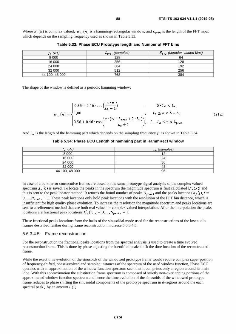
ETSI
ETSI TS 103 634 V1.1.1 (2019-08)88
Where &%( ) is complex valued, ���(�) is a hamming-rectangular window, and ����� is the length of the FFT input which depends on the sampling frequency used as shown in Table 5.33.
Table 5.33: Phase ECU Prototype length and Number of FFT bins
�� (Hz) ����� (samples) ���� (complex valued bins) 8 000 128 64
16 000 256 128 24 000 384 192 32 000 512 256
44 100, 48 000 768 384
The shape of the window is defined as a periodic hamming window:
������ =
⎩⎪⎨⎪⎧ 0,56 + 0,46 ∙ cos + , ∙ ��� + 1
- , 0 ≤ � < ��1,00 , �� ≤ � < � − ��0,56 + 0,46 ∙ cos., ∙ /� − ����� + 2 ∙ ��0�� + 1
1 , � − �� ≤ � < ������212�
And �� is the length of the hamming part which depends on the sampling frequency � as shown in Table 5.34.
Table 5.34: Phase ECU Length of hamming part in HammRect window
�� (Hz) �� (samples) 8 000 12
16 000 24 24 000 36 32 000 48
44 100, 48 000 96
In case of a burst error consecutive frames are based on the same prototype signal analysis so the complex valued spectrum ��(�) is saved. To locate the peaks in the spectrum the magnitude spectrum is first calculated |��(�)| and this is sent to the peak locator method. It returns the found number of peaks ������ and the peaks locations �����, � =
0, … , ������ − 1. These peak locations only hold peak locations with the resolution of the FFT bin distance, which is insufficient for high quality phase evolution. To increase the resolution the magnitude spectrum and peaks locations are sent to a refinement method that use both real valued or complex valued interpolation. After the interpolation the peaks locations are fractional peak locations �′����, � = 0, … , ������ − 1.
These fractional peaks locations form the basis of the sinusoidal mode used for the reconstructions of the lost audio frames described further during frame reconstruction in clause 5.6.3.4.5.
5.6.3.4.5 Frame reconstruction
For the reconstruction the fractional peaks locations from the spectral analysis is used to create a time evolved reconstruction frame. This is done by phase adjusting the identified peaks to fit the time location of the reconstructed frame.
While the exact time evolution of the sinusoids of the windowed prototype frame would require complex super position of frequency-shifted, phase-evolved and sampled instances of the spectrum of the used window function, Phase ECU operates with an approximation of the window function spectrum such that it comprises only a region around its main lobe. With this approximation the substitution frame spectrum is composed of strictly non-overlapping portions of the approximated window function spectrum and hence the time evolution of the sinusoids of the windowed prototype frame reduces to phase shifting the sinusoidal components of the prototype spectrum in �-regions around the each spectral peak � by an amount (�).
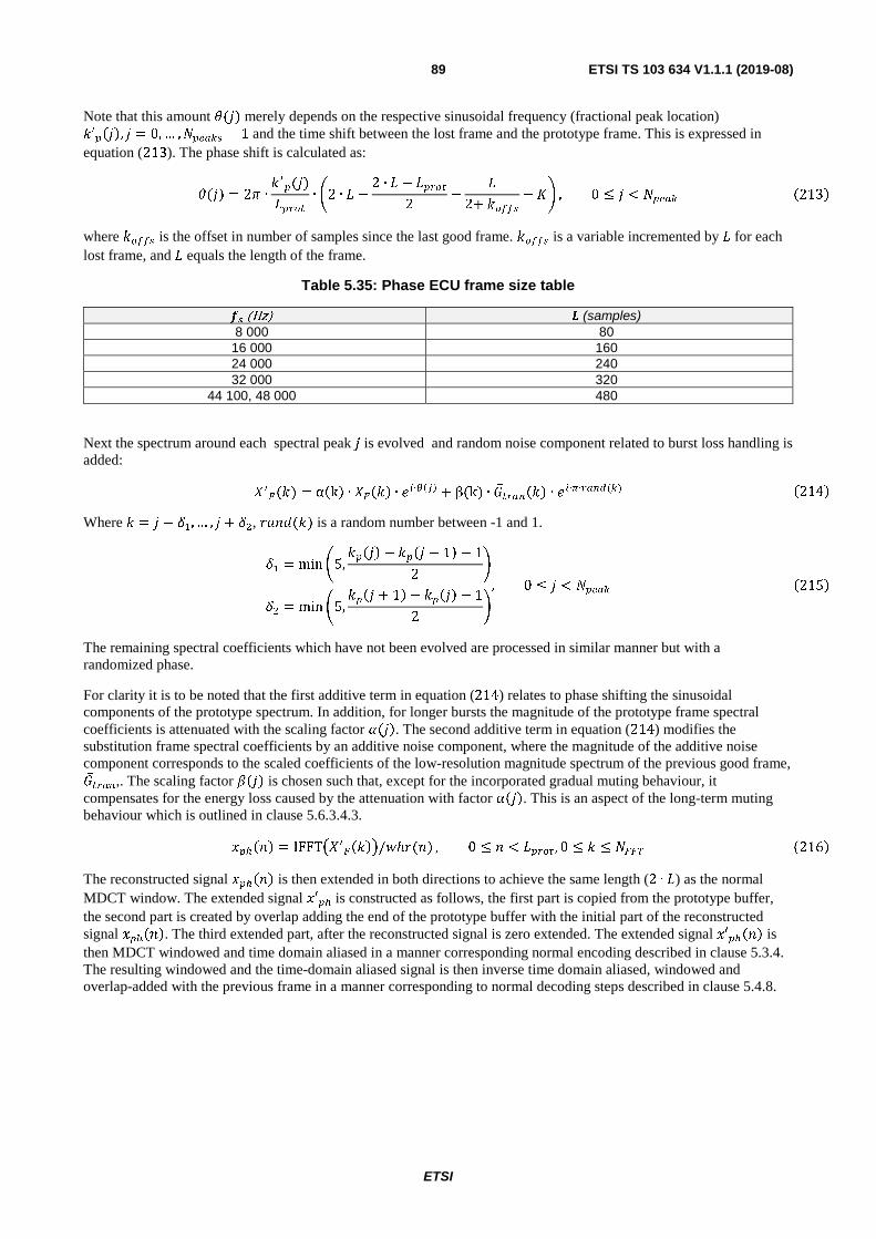
ETSI
ETSI TS 103 634 V1.1.1 (2019-08)89
Note that this amount (�) merely depends on the respective sinusoidal frequency (fractional peak location) �′����, � = 0, … , ������ − 1 and the time shift between the lost frame and the prototype frame. This is expressed in equation (213). The phase shift is calculated as:
(�) = 2 ∙���(�)��� ∙ �2 ∙ � −
2 ∙ � − ���2
−�
2+ ���� − � , 0 ≤ � < ����� �213�
where ���� is the offset in number of samples since the last good frame. ���� is a variable incremented by � for each lost frame, and � equals the length of the frame.
Table 5.35: Phase ECU frame size table
�� (Hz) � (samples) 8 000 80
16 000 160 24 000 240 32 000 320
44 100, 48 000 480
Next the spectrum around each spectral peak � is evolved and random noise component related to burst loss handling is added:
���(�) = α�k� ∙ ����� ∙ ��∙ ��� + β(k) ∙ �̅������ ∙ ��∙�∙����(�) �214�
Where � = � − ��, … , � + ��, ����(�) is a random number between -1 and 1.
�� = min �5,����� − ���� − 1� − 1
2�
�� = min �5,���� + 1� − ����� − 1
2�, 0 ≤ � < ����� �215�
The remaining spectral coefficients which have not been evolved are processed in similar manner but with a randomized phase.
For clarity it is to be noted that the first additive term in equation (214) relates to phase shifting the sinusoidal components of the prototype spectrum. In addition, for longer bursts the magnitude of the prototype frame spectral coefficients is attenuated with the scaling factor ����. The second additive term in equation (214) modifies the substitution frame spectral coefficients by an additive noise component, where the magnitude of the additive noise component corresponds to the scaled coefficients of the low-resolution magnitude spectrum of the previous good frame, �̅���,. The scaling factor ���� is chosen such that, except for the incorporated gradual muting behaviour, it compensates for the energy loss caused by the attenuation with factor ����. This is an aspect of the long-term muting behaviour which is outlined in clause 5.6.3.4.3.
������ = IFFT��������/�ℎ�(�) , 0 ≤ � < ��� , 0 ≤ � ≤ ���� �216�
The reconstructed signal ������ is then extended in both directions to achieve the same length (2 ∙ �) as the normal MDCT window. The extended signal �′�� is constructed as follows, the first part is copied from the prototype buffer, the second part is created by overlap adding the end of the prototype buffer with the initial part of the reconstructed signal ������. The third extended part, after the reconstructed signal is zero extended. The extended signal �′����� is then MDCT windowed and time domain aliased in a manner corresponding normal encoding described in clause 5.3.4. The resulting windowed and the time-domain aliased signal is then inverse time domain aliased, windowed and overlap-added with the previous frame in a manner corresponding to normal decoding steps described in clause 5.4.8.
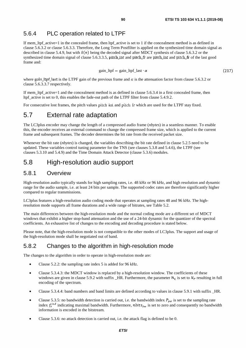
ETSI
ETSI TS 103 634 V1.1.1 (2019-08)90
5.6.4 PLC operation related to LTPF
If mem_ltpf_active=1 in the concealed frame, then ltpf_active is set to 1 if the concealment method is as defined in clause 5.6.3.2 or clause 5.6.3.3. Therefore, the Long Term Postfilter is applied on the synthesized time domain signal as described in clause 5.4.9, but with ����� being the decoded signal after MDCT synthesis of clause 5.6.3.2 or the synthesized time domain signal of clause 5.6.3.3.5, pitch_int and pitch_fr are pitch_int and pitch_fr of the last good frame and:
gain_ltpf = gain_ltpf_last ∙ � �217�
where gain_ltpf_last is the LTPF gain of the previous frame and � is the attenuation factor from clause 5.6.3.2 or clause 5.6.3.3.7 respectively.
If mem_ltpf_active=1 and the concealment method is as defined in clause 5.6.3.4 in a first concealed frame, then ltpf_active is set to 0, this enables the fade-out path of the LTPF filter from clause 5.4.9.2.
For consecutive lost frames, the pitch values pitch_int and pitch_fr which are used for the LTPF stay fixed.
5.7 External rate adaptation The LC3plus encoder may change the length of a compressed audio frame (nbytes) in a seamless manner. To enable this, the encoder receives an external command to change the compressed frame size, which is applied to the current frame and subsequent frames. The decoder determines the bit rate from the received packet size.
Whenever the bit rate (nbytes) is changed, the variables describing the bit rate defined in clause 5.2.5 need to be updated. These variables control tuning parameter for the TNS (see clauses 5.3.8 and 5.4.6), the LTPF (see clauses 5.3.10 and 5.4.9) and the Time Domain Attack Detector (clause 5.3.6) modules.
5.8 High-resolution audio support
5.8.1 Overview
High-resolution audio typically stands for high sampling rates, i.e. 48 kHz or 96 kHz, and high resolution and dynamic range for the audio sample, i.e. at least 24 bits per sample. The supported codec rates are therefore significantly higher compared to regular transmissions.
LC3plus features a high-resolution audio coding mode that operates at sampling rates 48 and 96 kHz. The high-resolution mode supports all frame durations and a wide range of bitrates, see Table 5.2.
The main differences between the high-resolution mode and the normal coding mode are a different set of MDCT windows that exhibit a higher stop-band attenuation and the use of a 24-bit dynamic for the quantizer of the spectral coefficients. An exhaustive list of changes to the encoding and decoding procedure is stated below.
Please note, that the high-resolution mode is not compatible to the other modes of LC3plus. The support and usage of the high-resolution mode shall be negotiated out of band.
5.8.2 Changes to the algorithm in high-resolution mode
The changes to the algorithm in order to operate in high-resolution mode are:
• Clause 5.2.2: the sampling rate index 5 is added for 96 kHz.
• Clause 5.3.4.3: the MDCT window is replaced by a high-resolution window. The coefficients of these windows are given in clause 5.9.2 with suffix _HR. Furthermore, the parameter N� is set to �� resulting in full encoding of the spectrum.
• Clause 5.3.4.4: band numbers and band limits are defined according to values in clause 5.9.1 with suffix _HR.
• Clause 5.3.5: no bandwidth detection is carried out, i.e. the bandwidth index ��� is set to the sampling rate index ����� indicating maximal bandwidth. Furthermore, �� !"�� is set to zero and consequently no bandwidth information is encoded in the bitstream.
• Clause 5.3.6: no attack detection is carried out, i.e. the attack flag is defined to be 0.
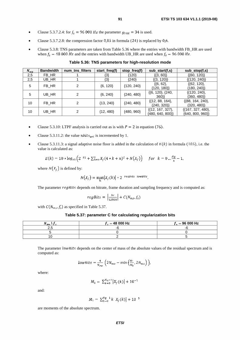
ETSI
ETSI TS 103 634 V1.1.1 (2019-08)91
• Clause 5.3.7.2.4: for �� = 96 000 #$ the parameter %��� = 34 is used.
• Clause 5.3.7.2.8: the compression factor 0,85 in formula �24� is replaced by 0,6.
• Clause 5.3.8: TNS parameters are taken from Table 5.36 where the entries with bandwidth FB_HR are used when �� = 48 000 #$ and the entries with bandwidth UB_HR are used when �� = 96 000 #$.
Table 5.36: TNS parameters for high-resolution mode
��� Bandwidth num_tns_filters start_freq(f) stop_freq(f) sub_start(f,s) sub_stop(f,s) 2,5 FB_HR 1 {3} {120} {{3, 60}} {{60, 120}} 2,5 UB_HR 1 {3} {240} {{3, 120}} {{120, 240}}
5 FB_HR 2 {6, 120} {120, 240} {{6, 62}, {120, 180}}
{{62, 120}, {180, 240}}
5 UB_HR 2 {6, 240} {240, 480} {{6, 120}, {240, 360}}
{{120, 240}, {360, 480}}
10 FB_HR 2 {13, 240} {240, 480} {{12, 88, 164}, {240, 320}}
{{88, 164, 240}, {320, 480}}
10 UB_HR 2 {12, 480} {480, 960} {{12, 167, 327}, {480, 640, 800}}
{{167, 327, 480}, {640, 800, 960}}
• Clause 5.3.10: LTPF analysis is carried out as is with � = 2 in equation �76�.
• Clause 5.3.11.2: the value �� !"��� is incremented by 1.
• Clause 5.3.11.3: a signal adaptive noise floor is added in the calculation of &��� in formula �105�, i.e. the value is calculated as:
&��� = 10 ∗ log�� '2��� + ∑ ���4 ∗ � + ������� + �����) �*� � = 0 …
�
!− 1,
where ����� is defined by:
����� = max"
+��(�)+ ∗ 2���#$�����$�� .
The parameter ��%, !" depends on bitrate, frame duration and sampling frequency and is computed as:
��%, !" = - ��
��%��. + /(�&� , ��)
with /��&� , ��� as specified in Table 5.37.
Table 5.37: parameter C for calculating regularization bits
��� \ �� �� = 48 000 Hz �� = 96 000 Hz 2,5 -6 -6 5 0 0 10 2 5
The parameter 0*�, !" depends on the center of mass of the absolute values of the residual spectrum and is computed as:
0*�, !" =!
�� '2�&� − min ''�
'�, 2�&�) ),
where:
1� = ∑ +��(�)+ ���
��� + 10�%
and:
1� = ∑ � +��(�)+ ���
��� + 10�%
are moments of the absolute spectrum.
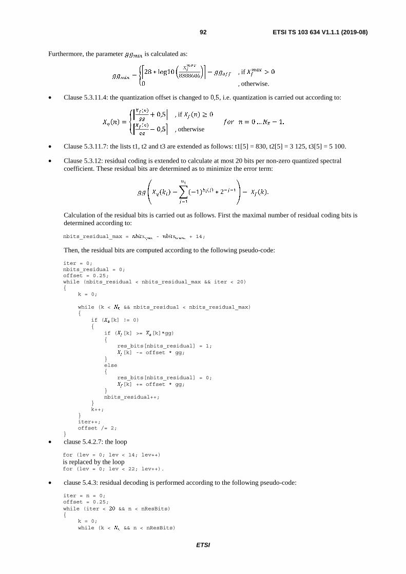
ETSI
ETSI TS 103 634 V1.1.1 (2019-08)92
Furthermore, the parameter %%&�� is calculated as:
%%&�� = 2328 ∗ log10 4 (����
838860656 − %%�� , if ��&�) > 0
0 , otherwise.
• Clause 5.3.11.4: the quantization offset is changed to 0,5, i.e. quantization is carried out according to:
�*��� = 7-(����##
+ 0,5. , if ����� ≥ 0
8(����##
− 0,59 , otherwise �*� � = 0 … �+ − 1.
• Clause 5.3.11.7: the lists t1, t2 and t3 are extended as follows: t1[5] = 830, t2[5] = 3 125, t3[5] = 5 100.
• Clause 5.3.12: residual coding is extended to calculate at most 20 bits per non-zero quantized spectral coefficient. These residual bits are determined as to minimize the error term:
%% :�*���� − ;�−1����� ∗ 2����
�
���
< − �����.
Calculation of the residual bits is carried out as follows. First the maximal number of residual coding bits is determined according to:
nbits_residual_max = ��������� - ���������� + 14;
Then, the residual bits are computed according to the following pseudo-code:
iter = 0; nbits_residual = 0; offset = 0.25; while (nbits_residual < nbits_residual_max && iter < 20) { k = 0; while (k < � && nbits_residual < nbits_residual_max) { if (�[k] != 0) { if (��[k] >= �[k]*gg) { res_bits[nbits_residual] = 1; ��[k] -= offset * gg; } else { res_bits[nbits_residual] = 0; ��[k] += offset * gg; } nbits_residual++; } k++; } iter++; offset /= 2; }
• clause 5.4.2.7: the loop
for (lev = 0; lev < 14; lev++) is replaced by the loop for (lev = 0; lev < 22; lev++).
• clause 5.4.3: residual decoding is performed according to the following pseudo-code:
iter = n = 0; offset = 0.25; while (iter < 20 && n < nResBits) { k = 0; while (k < � && n < nResBits)
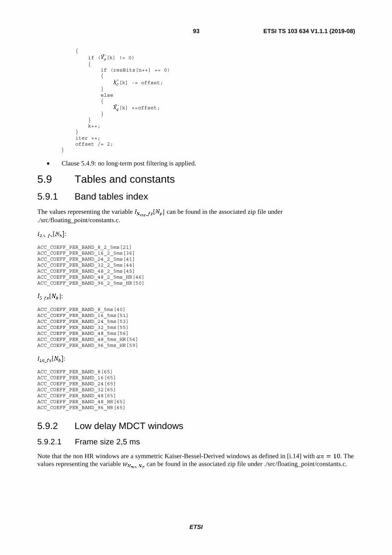
ETSI
ETSI TS 103 634 V1.1.1 (2019-08)93
{ if (��[k] != 0) { if (resBits[n++] == 0) { �
�[k] -= offset; }
else { �
�[k] +=offset; } } k++; } iter ++; offset /= 2; }
• Clause 5.4.9: no long-term post filtering is applied.
5.9 Tables and constants
5.9.1 Band tables index
The values representing the variable = ��_��[��] can be found in the associated zip file under
./src/floating_point/constants.c.
=�.%_��[��]:
ACC_COEFF_PER_BAND_8_2_5ms[21] ACC_COEFF_PER_BAND_16_2_5ms[36] ACC_COEFF_PER_BAND_24_2_5ms[41] ACC_COEFF_PER_BAND_32_2_5ms[44] ACC_COEFF_PER_BAND_48_2_5ms[45] ACC_COEFF_PER_BAND_48_2_5ms_HR[46] ACC_COEFF_PER_BAND_96_2_5ms_HR[50] =%_��[��]:
ACC_COEFF_PER_BAND_8_5ms[40] ACC_COEFF_PER_BAND_16_5ms[51] ACC_COEFF_PER_BAND_24_5ms[53] ACC_COEFF_PER_BAND_32_5ms[55] ACC_COEFF_PER_BAND_48_5ms[56] ACC_COEFF_PER_BAND_48_5ms_HR[56] ACC_COEFF_PER_BAND_96_5ms_HR[59] =��_��[��]:
ACC_COEFF_PER_BAND_8[65] ACC_COEFF_PER_BAND_16[65] ACC_COEFF_PER_BAND_24[65] ACC_COEFF_PER_BAND_32[65] ACC_COEFF_PER_BAND_48[65] ACC_COEFF_PER_BAND_48_HR[65] ACC_COEFF_PER_BAND_96_HR[65]
5.9.2 Low delay MDCT windows
5.9.2.1 Frame size 2,5 ms
Note that the non HR windows are a symmetric Kaiser-Bessel-Derived windows as defined in [i.14] with � = 10. The values representing the variable � ��_
can be found in the associated zip file under ./src/floating_point/constants.c.
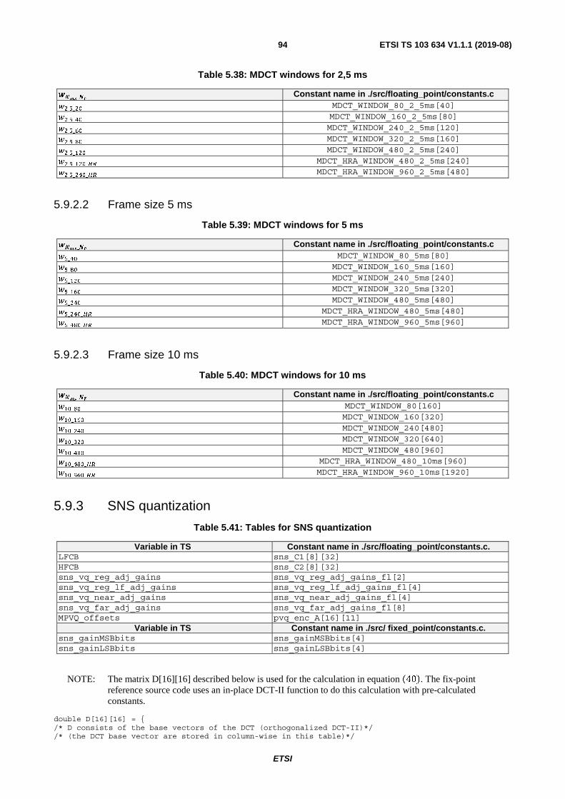
ETSI
ETSI TS 103 634 V1.1.1 (2019-08)94
Table 5.38: MDCT windows for 2,5 ms
����
_�� Constant name in ./src/floating_point/constants.c
��.�_�� MDCT_WINDOW_80_2_5ms[40]
��.�_�� MDCT_WINDOW_160_2_5ms[80]
��.�_�� MDCT_WINDOW_240_2_5ms[120]
��.�_�� MDCT_WINDOW_320_2_5ms[160]
��.�_��� MDCT_WINDOW_480_2_5ms[240]
��.�_���_ MDCT_HRA_WINDOW_480_2_5ms[240]
��.�_���_ MDCT_HRA_WINDOW_960_2_5ms[480]
5.9.2.2 Frame size 5 ms
Table 5.39: MDCT windows for 5 ms
����_�� Constant name in ./src/floating_point/constants.c
��_�� MDCT_WINDOW_80_5ms[80]
��_�� MDCT_WINDOW_160_5ms[160]
��_��� MDCT_WINDOW_240_5ms[240]
��_��� MDCT_WINDOW_320_5ms[320]
��_��� MDCT_WINDOW_480_5ms[480]
��_���_ MDCT_HRA_WINDOW_480_5ms[480]
��_���_ MDCT_HRA_WINDOW_960_5ms[960]
5.9.2.3 Frame size 10 ms
Table 5.40: MDCT windows for 10 ms
����_�� Constant name in ./src/floating_point/constants.c
���_�� MDCT_WINDOW_80[160]
���_��� MDCT_WINDOW_160[320]
���_��� MDCT_WINDOW_240[480]
���_��� MDCT_WINDOW_320[640]
���_��� MDCT_WINDOW_480[960]
���_���_ MDCT_HRA_WINDOW_480_10ms[960]
���_���_ MDCT_HRA_WINDOW_960_10ms[1920]
5.9.3 SNS quantization
Table 5.41: Tables for SNS quantization
Variable in TS Constant name in ./src/floating_point/constants.c. LFCB sns_C1[8][32] HFCB sns_C2[8][32] sns_vq_reg_adj_gains sns_vq_reg_adj_gains_fl[2] sns_vq_reg_lf_adj_gains sns_vq_reg_lf_adj_gains_fl[4] sns_vq_near_adj_gains sns_vq_near_adj_gains_fl[4] sns_vq_far_adj_gains sns_vq_far_adj_gains_fl[8] MPVQ_offsets pvq_enc_A[16][11]
Variable in TS Constant name in ./src/ fixed_point/constants.c. sns_gainMSBbits sns_gainMSBbits[4] sns_gainLSBbits sns_gainLSBbits[4]
NOTE: The matrix D[16][16] described below is used for the calculation in equation �40�. The fix-point reference source code uses an in-place DCT-II function to do this calculation with pre-calculated constants.
double D[16][16] = { /* D consists of the base vectors of the DCT (orthogonalized DCT-II)*/ /* (the DCT base vector are stored in column-wise in this table)*/
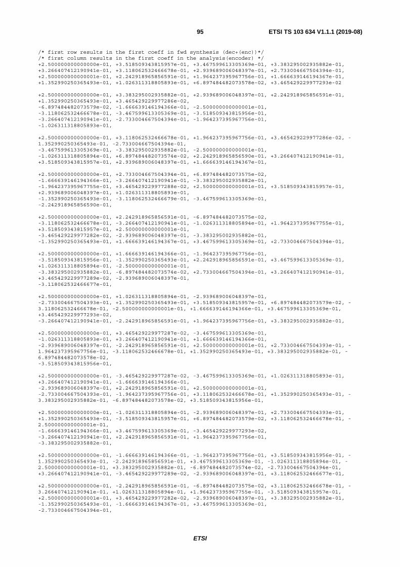
ETSI
ETSI TS 103 634 V1.1.1 (2019-08)95
/* first row results in the first coeff in fwd synthesis (dec+(enc))*/ /* first column results in the first coeff in the analysis(encoder) */ +2.500000000000000e-01, +3.518509343815957e-01, +3.467599613305369e-01, +3.383295002935882e-01, +3.266407412190941e-01, +3.118062532466678e-01, +2.939689006048397e-01, +2.733004667504394e-01, +2.500000000000001e-01, +2.242918965856591e-01, +1.964237395967756e-01, +1.666639146194367e-01, +1.352990250365493e-01, +1.026311318805893e-01, +6.897484482073578e-02, +3.465429229977293e-02 +2.500000000000000e-01, +3.383295002935882e-01, +2.939689006048397e-01, +2.242918965856591e-01, +1.352990250365493e-01, +3.465429229977286e-02, -6.897484482073579e-02, -1.666639146194366e-01, -2.500000000000001e-01, -3.118062532466678e-01, -3.467599613305369e-01, -3.518509343815956e-01, -3.266407412190941e-01, -2.733004667504394e-01, -1.964237395967756e-01, -1.026311318805893e-01, +2.500000000000000e-01, +3.118062532466678e-01, +1.964237395967756e-01, +3.465429229977286e-02, -1.352990250365493e-01, -2.733004667504394e-01, -3.467599613305369e-01, -3.383295002935882e-01, -2.500000000000001e-01, -1.026311318805894e-01, +6.897484482073574e-02, +2.242918965856590e-01, +3.266407412190941e-01, +3.518509343815957e-01, +2.939689006048397e-01, +1.666639146194367e-01, +2.500000000000000e-01, +2.733004667504394e-01, +6.897484482073575e-02, -1.666639146194366e-01, -3.266407412190941e-01, -3.383295002935882e-01, -1.964237395967755e-01, +3.465429229977288e-02, +2.500000000000001e-01, +3.518509343815957e-01, +2.939689006048397e-01, +1.026311318805893e-01, -1.352990250365493e-01, -3.118062532466679e-01, -3.467599613305369e-01, -2.242918965856590e-01, +2.500000000000000e-01, +2.242918965856591e-01, -6.897484482073575e-02, -3.118062532466678e-01, -3.266407412190941e-01, -1.026311318805894e-01, +1.964237395967755e-01, +3.518509343815957e-01, +2.500000000000001e-01, -3.465429229977282e-02, -2.939689006048397e-01, -3.383295002935882e-01, -1.352990250365493e-01, +1.666639146194367e-01, +3.467599613305369e-01, +2.733004667504394e-01, +2.500000000000000e-01, +1.666639146194366e-01, -1.964237395967756e-01, -3.518509343815956e-01, -1.352990250365493e-01, +2.242918965856591e-01, +3.467599613305369e-01, +1.026311318805894e-01, -2.500000000000001e-01, -3.383295002935882e-01, -6.897484482073574e-02, +2.733004667504394e-01, +3.266407412190941e-01, +3.465429229977289e-02, -2.939689006048397e-01, -3.118062532466677e-01, +2.500000000000000e-01, +1.026311318805894e-01, -2.939689006048397e-01, -2.733004667504393e-01, +1.352990250365493e-01, +3.518509343815957e-01, +6.897484482073579e-02, -3.118062532466678e-01, -2.500000000000001e-01, +1.666639146194366e-01, +3.467599613305369e-01, +3.465429229977293e-02, -3.266407412190941e-01, -2.242918965856591e-01, +1.964237395967756e-01, +3.383295002935882e-01, +2.500000000000000e-01, +3.465429229977287e-02, -3.467599613305369e-01, -1.026311318805893e-01, +3.266407412190941e-01, +1.666639146194366e-01, -2.939689006048397e-01, -2.242918965856591e-01, +2.500000000000001e-01, +2.733004667504393e-01, -1.964237395967756e-01, -3.118062532466678e-01, +1.352990250365493e-01, +3.383295002935882e-01, -6.897484482073578e-02, -3.518509343815956e-01, +2.500000000000000e-01, -3.465429229977287e-02, -3.467599613305369e-01, +1.026311318805893e-01, +3.266407412190941e-01, -1.666639146194366e-01, -2.939689006048397e-01, +2.242918965856591e-01, +2.500000000000001e-01, -2.733004667504393e-01, -1.964237395967756e-01, +3.118062532466678e-01, +1.352990250365493e-01, -3.383295002935882e-01, -6.897484482073578e-02, +3.518509343815956e-01, +2.500000000000000e-01, -1.026311318805894e-01, -2.939689006048397e-01, +2.733004667504393e-01, +1.352990250365493e-01, -3.518509343815957e-01, +6.897484482073579e-02, +3.118062532466678e-01, -2.500000000000001e-01, -1.666639146194366e-01, +3.467599613305369e-01, -3.465429229977293e-02, -3.266407412190941e-01, +2.242918965856591e-01, +1.964237395967756e-01, -3.383295002935882e-01, +2.500000000000000e-01, -1.666639146194366e-01, -1.964237395967756e-01, +3.518509343815956e-01, -1.352990250365493e-01, -2.242918965856591e-01, +3.467599613305369e-01, -1.026311318805894e-01, -2.500000000000001e-01, +3.383295002935882e-01, -6.897484482073574e-02, -2.733004667504394e-01, +3.266407412190941e-01, -3.465429229977289e-02, -2.939689006048397e-01, +3.118062532466677e-01, +2.500000000000000e-01, -2.242918965856591e-01, -6.897484482073575e-02, +3.118062532466678e-01, -3.266407412190941e-01, +1.026311318805894e-01, +1.964237395967755e-01, -3.518509343815957e-01, +2.500000000000001e-01, +3.465429229977282e-02, -2.939689006048397e-01, +3.383295002935882e-01, -1.352990250365493e-01, -1.666639146194367e-01, +3.467599613305369e-01, -2.733004667504394e-01,
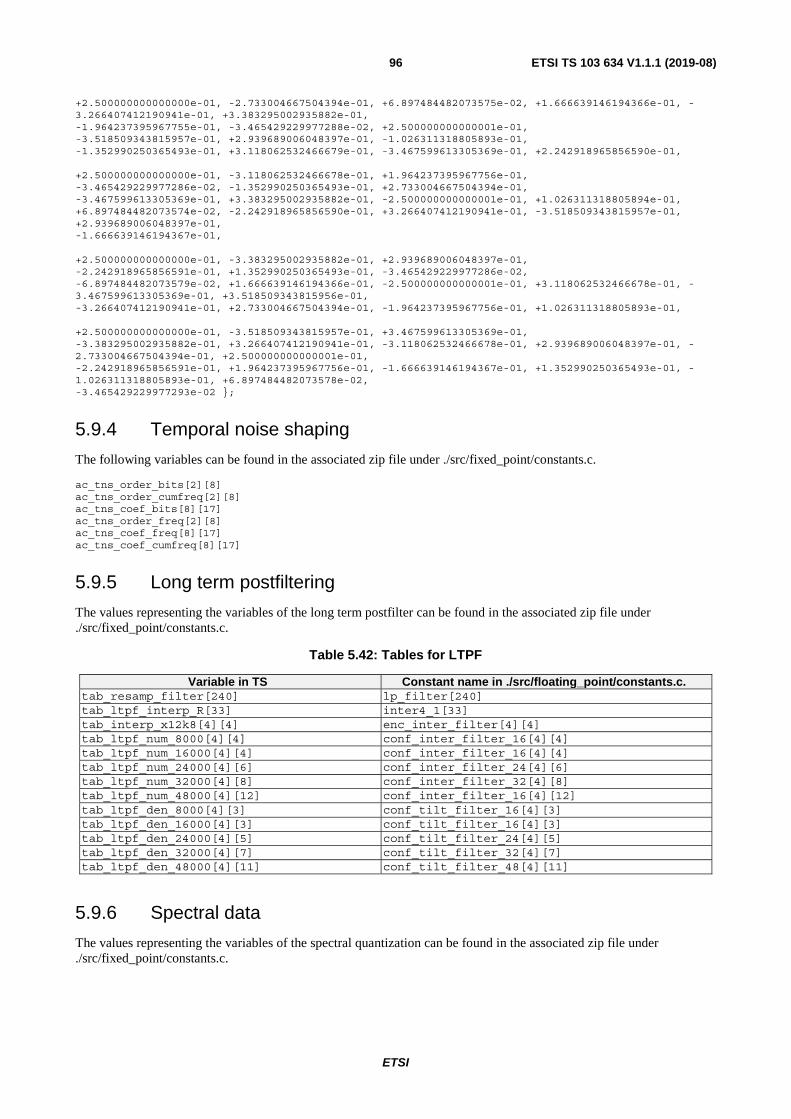
ETSI
ETSI TS 103 634 V1.1.1 (2019-08)96
+2.500000000000000e-01, -2.733004667504394e-01, +6.897484482073575e-02, +1.666639146194366e-01, -3.266407412190941e-01, +3.383295002935882e-01, -1.964237395967755e-01, -3.465429229977288e-02, +2.500000000000001e-01, -3.518509343815957e-01, +2.939689006048397e-01, -1.026311318805893e-01, -1.352990250365493e-01, +3.118062532466679e-01, -3.467599613305369e-01, +2.242918965856590e-01, +2.500000000000000e-01, -3.118062532466678e-01, +1.964237395967756e-01, -3.465429229977286e-02, -1.352990250365493e-01, +2.733004667504394e-01, -3.467599613305369e-01, +3.383295002935882e-01, -2.500000000000001e-01, +1.026311318805894e-01, +6.897484482073574e-02, -2.242918965856590e-01, +3.266407412190941e-01, -3.518509343815957e-01, +2.939689006048397e-01, -1.666639146194367e-01, +2.500000000000000e-01, -3.383295002935882e-01, +2.939689006048397e-01, -2.242918965856591e-01, +1.352990250365493e-01, -3.465429229977286e-02, -6.897484482073579e-02, +1.666639146194366e-01, -2.500000000000001e-01, +3.118062532466678e-01, -3.467599613305369e-01, +3.518509343815956e-01, -3.266407412190941e-01, +2.733004667504394e-01, -1.964237395967756e-01, +1.026311318805893e-01, +2.500000000000000e-01, -3.518509343815957e-01, +3.467599613305369e-01, -3.383295002935882e-01, +3.266407412190941e-01, -3.118062532466678e-01, +2.939689006048397e-01, -2.733004667504394e-01, +2.500000000000001e-01, -2.242918965856591e-01, +1.964237395967756e-01, -1.666639146194367e-01, +1.352990250365493e-01, -1.026311318805893e-01, +6.897484482073578e-02, -3.465429229977293e-02 };
5.9.4 Temporal noise shaping
The following variables can be found in the associated zip file under ./src/fixed_point/constants.c.
ac_tns_order_bits[2][8] ac_tns_order_cumfreq[2][8] ac_tns_coef_bits[8][17] ac_tns_order_freq[2][8] ac_tns_coef_freq[8][17] ac_tns_coef_cumfreq[8][17]
5.9.5 Long term postfiltering
The values representing the variables of the long term postfilter can be found in the associated zip file under ./src/fixed_point/constants.c.
Table 5.42: Tables for LTPF
Variable in TS Constant name in ./src/floating_point/constants.c. tab_resamp_filter[240] lp_filter[240] tab_ltpf_interp_R[33] inter4_1[33] tab_interp_x12k8[4][4] enc_inter_filter[4][4] tab_ltpf_num_8000[4][4] conf_inter_filter_16[4][4] tab_ltpf_num_16000[4][4] conf_inter_filter_16[4][4] tab_ltpf_num_24000[4][6] conf_inter_filter_24[4][6] tab_ltpf_num_32000[4][8] conf_inter_filter_32[4][8] tab_ltpf_num_48000[4][12] conf_inter_filter_16[4][12] tab_ltpf_den_8000[4][3] conf_tilt_filter_16[4][3] tab_ltpf_den_16000[4][3] conf_tilt_filter_16[4][3] tab_ltpf_den_24000[4][5] conf_tilt_filter_24[4][5] tab_ltpf_den_32000[4][7] conf_tilt_filter_32[4][7] tab_ltpf_den_48000[4][11] conf_tilt_filter_48[4][11]
5.9.6 Spectral data
The values representing the variables of the spectral quantization can be found in the associated zip file under ./src/fixed_point/constants.c.
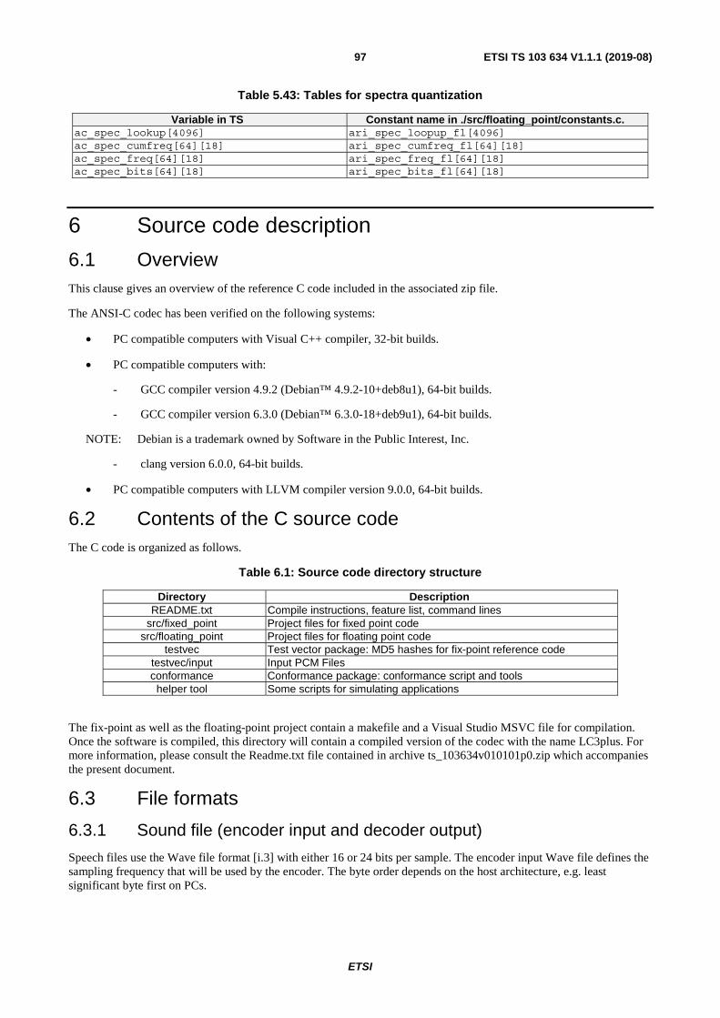
ETSI
ETSI TS 103 634 V1.1.1 (2019-08)97
Table 5.43: Tables for spectra quantization
Variable in TS Constant name in ./src/floating_point/constants.c. ac_spec_lookup[4096] ari_spec_loopup_fl[4096] ac_spec_cumfreq[64][18] ari_spec_cumfreq_fl[64][18] ac_spec_freq[64][18] ari_spec_freq_fl[64][18] ac_spec_bits[64][18] ari_spec_bits_fl[64][18]
6 Source code description
6.1 Overview This clause gives an overview of the reference C code included in the associated zip file.
The ANSI-C codec has been verified on the following systems:
• PC compatible computers with Visual C++ compiler, 32-bit builds.
• PC compatible computers with:
- GCC compiler version 4.9.2 (Debian™ 4.9.2-10+deb8u1), 64-bit builds.
- GCC compiler version 6.3.0 (Debian™ 6.3.0-18+deb9u1), 64-bit builds.
NOTE: Debian is a trademark owned by Software in the Public Interest, Inc.
- clang version 6.0.0, 64-bit builds.
• PC compatible computers with LLVM compiler version 9.0.0, 64-bit builds.
6.2 Contents of the C source code The C code is organized as follows.
Table 6.1: Source code directory structure
Directory Description README.txt Compile instructions, feature list, command lines
src/fixed_point Project files for fixed point code src/floating_point Project files for floating point code
testvec Test vector package: MD5 hashes for fix-point reference code testvec/input Input PCM Files conformance Conformance package: conformance script and tools
helper tool Some scripts for simulating applications
The fix-point as well as the floating-point project contain a makefile and a Visual Studio MSVC file for compilation. Once the software is compiled, this directory will contain a compiled version of the codec with the name LC3plus. For more information, please consult the Readme.txt file contained in archive ts_103634v010101p0.zip which accompanies the present document.
6.3 File formats
6.3.1 Sound file (encoder input and decoder output)
Speech files use the Wave file format [i.3] with either 16 or 24 bits per sample. The encoder input Wave file defines the sampling frequency that will be used by the encoder. The byte order depends on the host architecture, e.g. least significant byte first on PCs.
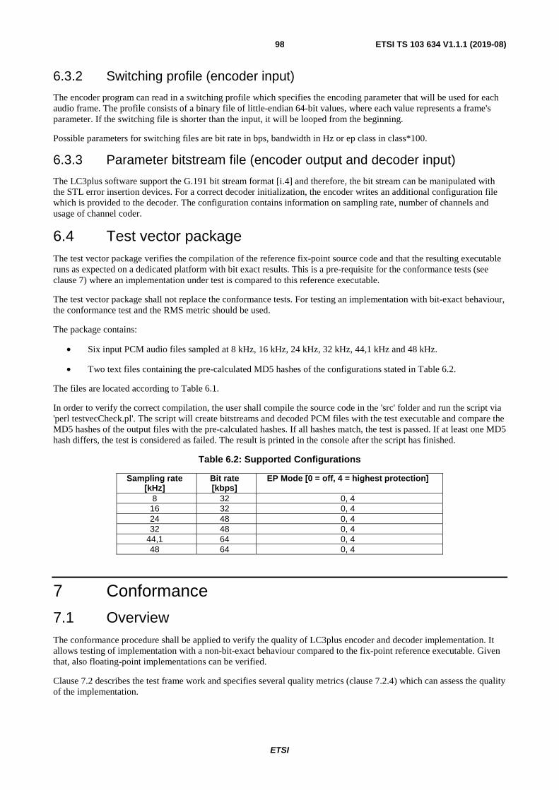
ETSI
ETSI TS 103 634 V1.1.1 (2019-08)98
6.3.2 Switching profile (encoder input)
The encoder program can read in a switching profile which specifies the encoding parameter that will be used for each audio frame. The profile consists of a binary file of little-endian 64-bit values, where each value represents a frame's parameter. If the switching file is shorter than the input, it will be looped from the beginning.
Possible parameters for switching files are bit rate in bps, bandwidth in Hz or ep class in class*100.
6.3.3 Parameter bitstream file (encoder output and decoder input)
The LC3plus software support the G.191 bit stream format [i.4] and therefore, the bit stream can be manipulated with the STL error insertion devices. For a correct decoder initialization, the encoder writes an additional configuration file which is provided to the decoder. The configuration contains information on sampling rate, number of channels and usage of channel coder.
6.4 Test vector package The test vector package verifies the compilation of the reference fix-point source code and that the resulting executable runs as expected on a dedicated platform with bit exact results. This is a pre-requisite for the conformance tests (see clause 7) where an implementation under test is compared to this reference executable.
The test vector package shall not replace the conformance tests. For testing an implementation with bit-exact behaviour, the conformance test and the RMS metric should be used.
The package contains:
• Six input PCM audio files sampled at 8 kHz, 16 kHz, 24 kHz, 32 kHz, 44,1 kHz and 48 kHz.
• Two text files containing the pre-calculated MD5 hashes of the configurations stated in Table 6.2.
The files are located according to Table 6.1.
In order to verify the correct compilation, the user shall compile the source code in the 'src' folder and run the script via 'perl testvecCheck.pl'. The script will create bitstreams and decoded PCM files with the test executable and compare the MD5 hashes of the output files with the pre-calculated hashes. If all hashes match, the test is passed. If at least one MD5 hash differs, the test is considered as failed. The result is printed in the console after the script has finished.
Table 6.2: Supported Configurations
Sampling rate [kHz]
Bit rate [kbps]
EP Mode [0 = off, 4 = highest protection]
8 32 0, 4 16 32 0, 4 24 48 0, 4 32 48 0, 4
44,1 64 0, 4 48 64 0, 4
7 Conformance
7.1 Overview The conformance procedure shall be applied to verify the quality of LC3plus encoder and decoder implementation. It allows testing of implementation with a non-bit-exact behaviour compared to the fix-point reference executable. Given that, also floating-point implementations can be verified.
Clause 7.2 describes the test frame work and specifies several quality metrics (clause 7.2.4) which can assess the quality of the implementation.

ETSI
ETSI TS 103 634 V1.1.1 (2019-08)99
Clause 7.3 defines several conformance tests grouped into core coder tests (clause 7.3.2), concealment tests (clause 7.3.3) and channel coder tests (clause 7.3.4). Most of the tests can be conducted by the modules (encoder, decoder and codec) (clause 7.2.3) separately.
Clause 7.4 specifies which quality metric shall be used for a dedicated conformance tests and which modules shall be tested separately. Clause 7.5 defines the criteria for considering an implementation as conformant. Clause 7.7.2 gives an example for specifying conformance for specific applications.
The conformance scripts includes a reference implementation of the item preparation, core coder test, packet-loss tests and the channel coder tests. The conformance scripts is contained in archive ts_103634v010101p0.zip which accompanies the present document.
7.2 Test framework
7.2.1 Test material
A selection of nine items from the European Broadcasting Union Sound Quality Assessment Material EBU SQAM CD [7] shall be used. The material ensures testing of a wide range of LC3plus features. These items are trimmed according to Table 7.1.
Table 7.1: LC3plus Conformance Test Items
Track Name Track Number Start [s] Fragment Length [s] Used in PLC test ABBA 69 7 8 YES Castanets 27 0 8 YES Eddie_Rabbitt 70 0 8 NO Female_Speech_German 53 0 8 YES Glockenspiel 35 0 10 NO Harpsichord 40 39 9 YES Male_Speech_English 50 0 8 YES Piano_Schubert 60 0 8 NO Violoncello 10 0 10 NO
For all items, a fade-in of 0,5 s and a fade-out of 0,7 s is chosen. Please refer to the LC3plus Conformance Script (clause 7.2.5.6) for the command lines used for pre-processing the test items. Note that a subsection of these items is used for the PLC test.
7.2.2 Test permutations and codec parameters
The input items in combination with the codec parameters, e.g. bit rates, sampling rates, frame sizes, are permutated in order to create a set of test conditions. These permuted test conditions are used for each test unless stated otherwise.
For the channel coder tests, the parameters are in addition permutated with the five error protection (EP) modes (0, 1, 2, 3, 4).
The codec parameters depend on the application under test, e.g. 16 kHz sampling rate and bit rate 32 kbps for regular WB voice calls.
7.2.3 Modules under test
The conformance is applied for the following modules. Each module test creates two audio files which are further analysed by quality metrics in order to compare module under test and reference:
• Encoder under test (EuT): Items are encoded with the EuT and the reference encoder (ER) at all permutations and decoded with the reference coder (DR)
• Decoder under test (DuT): Items are encoded with the ER at all permutations and decoded with the DR and DuT
• Encoder-Decoder (EncDec): Items are encoded with the EuT and decoded with the DuT as well as encoded with the ER and decoded with the DR

ETSI
ETSI TS 103 634 V1.1.1 (2019-08)100
The reference executables/modules (DR and ER) shall be compiled without any modification of the reference source code and shall pass the testvector check outlined in clause 6.4.
7.2.4 Quality metric calculation
7.2.4.1 Root Mean Square
The RMS metric compares two time-domain signals and calculates its similarity in accuracy. The RMS level is calculated as follows:
��� � �1� �� �� � ��������
���
218�
where Out(n) denotes output signal under test, and Ref(n) denotes the reference signals for the comparison.
To fulfil the RMS/LSB Measurement test at an accuracy level of K bits, an LC3plus encoder and decoder shall provide an output waveform such that the RMS level of the difference signal between the output of the decoder under test and
the output of the reference decoder is less than �
����∙���.�. In addition, the difference signal shall have a maximum
absolute value of at most �
���� relative to full-scale. The RMS/LSB Measurement test shall be carried out for an
accuracy level of K=14 bit unless a different accuracy level is explicitly stated.
An RMS tool implementation is provided within the LC3plus conformance script package as C source code. This code can be compiled and the binary can be used to compare two audio files and calculate the overall RMS in dB, with the maximum absolute difference of two audio samples and the reached RMS criterion expressed in bits. The RMS tool can be used with the following command line:
./rms file1.wav file2.wav [k]
where k is an optional parameter to lower the conformance threshold in the range between 1 and 16 bits. Figure 7.1 illustrates the process and the calculation of the RMS value.
Figure 7.1: RMS calculation procedure for encoder, decoder and encdec Tests
NOTE: RMS might not be applicable for testing encoder implementations operating on different platforms, e.g. floating point. In that case Delta ODG is recommended.

ETSI
ETSI TS 103 634 V1.1.1 (2019-08)101
7.2.4.2 Delta ODG value
To calculate the Objective Difference Grade (ODG) between two audio files, an ITU-T BS.1387-1 (Advanced) implementation shall be used. The "Method for objective measurements of perceived audio quality" (BS.1387-1 Advanced) algorithm binary calculates the ODG between a coded audio file and the reference audio file. The ODG value is calculated for two files for each test permutation:
• ODG between reference audio and coded audio using LC3plus Reference codec
• ODG between reference audio and coded audio using LC3plus codec under test
The difference between the two ODGs (∆��) shall not exceed a certain threshold according to clause 7.2.4.3. Figure 7.2 illustrates the coding process and the calculation of ∆�� for Encoder, Decoder and EncDec Tests.
Figure 7.2: ∆ODG calculation procedure for encoder, decoder and encdec tests
7.2.4.3 Maximum loudness difference (MLD)
The MLD value is calculated for two decoded files for each test permutation according to [i.7]. The following steps according to Recommendation ITU-R BS.1387-1 [i.11] need to be processed first:
• Filterbank (Annex 2 clause 2.2.5 of [i.11]):
- subsample factor F changed to 16 for higher time resolution.
• Outer and Middle Ear Filtering (Annex 2 clause 2.2.6 of [i.11])
• Frequency Domain Smearing (Annex 2 clause 2.2.7 of [i.11])
• Rectification (Annex 2 clause 2.2.8 of [i.11])
• Time Domain Smearing 1 - Backward Masking (Annex 2 clause 2.2.9 of [i.11])
• Adding of Internal Noise (Annex 2 clause 2.2.10 of [i.11])
• Time Domain Smearing 2 - Forward Masking (Annex 2 clause 2.2.11 of [i.11])
• Loudness (Annex 2 clause 3.3 of [i.11]):
- This section defines the specific loudness patterns ���, �� for � subbands and � time samples
- The specific loudness patterns are calculated for:
reference signal �����, �� signal under test � �� ��, ��
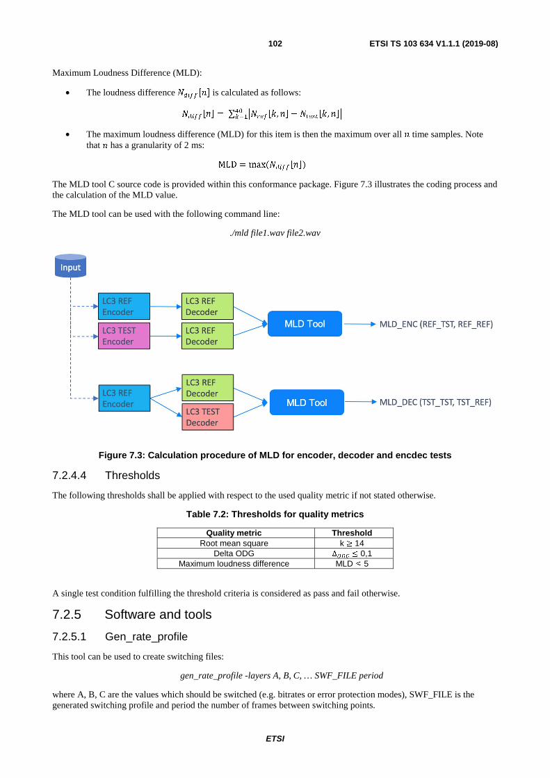
ETSI
ETSI TS 103 634 V1.1.1 (2019-08)102
Maximum Loudness Difference (MLD):
• The loudness difference �������� is calculated as follows:
�������� � ∑ ������, �� � � �� ��, ��������
• The maximum loudness difference (MLD) for this item is then the maximum over all � time samples. Note that � has a granularity of 2 ms:
MLD � max ��������� The MLD tool C source code is provided within this conformance package. Figure 7.3 illustrates the coding process and the calculation of the MLD value.
The MLD tool can be used with the following command line:
./mld file1.wav file2.wav
Figure 7.3: Calculation procedure of MLD for encoder, decoder and encdec tests
7.2.4.4 Thresholds
The following thresholds shall be applied with respect to the used quality metric if not stated otherwise.
Table 7.2: Thresholds for quality metrics
Quality metric Threshold Root mean square k � 14
Delta ODG ∆��� � 0,1 Maximum loudness difference MLD � 5
A single test condition fulfilling the threshold criteria is considered as pass and fail otherwise.
7.2.5 Software and tools
7.2.5.1 Gen_rate_profile
This tool can be used to create switching files:
gen_rate_profile -layers A, B, C, … SWF_FILE period
where A, B, C are the values which should be switched (e.g. bitrates or error protection modes), SWF_FILE is the generated switching profile and period the number of frames between switching points.

ETSI
ETSI TS 103 634 V1.1.1 (2019-08)103
NOTE: For error protection switching files, the error protection mode is multiplied with a value of 100 in order to operate this tool.
7.2.5.2 Eid-xor
This tool can be used to introduce bit errors to a G.192 bitstream:
eid-xor -bs g192 in_bs error_pattern out_bs
where in_bs and out_bs are the input and output bitstreams both in the G.192 format [i.8] and error_pattern the error pattern in byte format.
7.2.5.3 flipG192
This tool can flip a number of bits in a number of frames in a G.192 bitstream. It is provided as C source code and is used for the error protection test with a correctable number of flipped bits. It can be used as follows:
flipG192 in_bs out_bs FLIPS FRAMES SEED VERBOSE
where in_bs and out_bs are the input and output bitstreams both in the G.192 format, FLIPS is the number of bits to flip in every frame, FRAMES is the number of frames to flip in percent, SEED is an integer seed for the random generator and VERBOSE specifies if the information about the flipped bits and the respective frames shall be shown (1) or not (0).
7.2.5.4 G.192 bitstream format
The test implementation shall be able to read and write a bitstream in the G.192 format [i.8]. All tests within this script use this format.
Each bit of the bitstream data is represented by a 16-bit word and is preceded by a synchronization word and the length word. A bit '0' is coded as the softbit '0x007F' and a bit '1' is coded as softbit '0x0081'. The synchronization word can take the following values:
• '0x6B21' representing a good frame
• '0x6B20' representing a bad/lost frame (bfi == 1)
• '0x6B22' representing a partially bad/lost frame (bfi == 2).
The length field contains the length (the total number of bits) as a 16-bit word.
7.2.5.5 Note to platform-dependent conformance
To prepare the audio samples for the conformance test, it is recommended to use SoX (Sound eXchange) [i.9] for any operations on the audio samples in order to prepare them for the conformance test. SoX behaves differently on different platforms, meaning that the same resampling operation on the same file will not be bit-exact if executed on different platforms. Therefore, to avoid such issues, it is recommended to use the SoX Windows-Binary (together with Wine [i.10] on non-Windows platforms) to avoid such issues.
7.2.5.6 Reference conformance test script
The conformance test script is a Python® script that implements all test procedures mentioned within the present document. It can be used on an operating system with Python3 installed:
lc3_conformance.py config.cfg [-v -w -keep]
where config.cfg is the configuration file containing all operation points to be tested. For detailed instructions and the prerequisites for running this script, please refer to the Readme.txt contained in archive ts_103634v010101p0.zip which accompanies the present document. An example configuration file is also provided within the example_config.cfg file.

ETSI
ETSI TS 103 634 V1.1.1 (2019-08)104
7.3 Conformance tests
7.3.1 Test groups
The LC3plus conformance tests are combined into the three groups:
• Core coder tests, see clause 7.3.2
• Concealment tests, see clause 7.3.3
• Channel coder tests, see clause 7.3.4
7.3.2 Core coder tests
7.3.2.1 SQAM test
The SQAM Test aims to verify the intrinsic audio quality of an implementation under test. It uses the nine prepared test items (Table 7.1) to provide audio quality metrics in comparison to the reference implementation.
Items are generated depending on the tested module according to clause 7.2.3. Quality metrics according to clause 7.4 are conducted.
7.3.2.2 Band limitation test
The band limitation test verifies the correct implementation of the bandwidth detector/limiter inside the LC3plus encoder and decoder. Therefore, the item Female_Speech_German from the EBU SQAM CD is resampled and low pass filtered to create the following test configurations:
Table 7.3: Test Configurations for Band Limitation Test
Sampling Rate [kHz] Bandwidth Bitrate [bytes / frame]
16 NB 40 24 NB, WB 60 32 NB, WB, SSWB 80 48 NB, WB, SSWB, SWB 115
Items are generated depending on the tested module according to clause 7.2.3. Quality metrics according to clause 7.4 are conducted.
7.3.2.3 Low pass test
The Low Pass Test shall verify the correct implementation of the cutoff frequency of 20 kHz used in the EuT. Therefore, the test is only relevant for sampling rates higher than 32 kHz. For this test, a signal consisting of white noise above 20 kHz is used. For this test, the energy difference ����� between the two output PCM files is calculated:
����� = 10 ∗ ������(��_��( ) − ��_��( ))�
�
��
�219�
����� should be below the limit of -20 dB, where N is the total number of audio samples.
Items are generated depending on the tested module according to clause 7.2.3. Quality metrics according to clause 7.4 are conducted.

ETSI
ETSI TS 103 634 V1.1.1 (2019-08)105
7.3.2.4 Bitrate switching test
The conformance tool shall be used for verifying the rate switching capability of the codec at runtime. It is required for the test implementation to accept a switching file instead of the bitrate parameter. The test implementation shall detect such a switching file and initialize the codec to the first bitrate from the bit rate switching file. The bitrate switching test is carried out for all frame sizes with the respective bitrate switching files and is following the same test procedure as outlined in the SQAM tests (clause 7.3.2.1).
Switching files are generated using the STL gen_rate_profile tool according to clause 7.2.5.1. The rate switching test generates one or more switching profiles and executes the SQAM test using the switching profiles instead of the bit rate. The switching file shall contain all required net bit rates according to the application.
Items are generated depending on the tested module according to clause 7.2.3. Quality metrics according to clause 7.4 are conducted.
7.3.2.5 Bandwidth switching test
The conformance tool shall be used for verifying the bandwidth switching capability of the codec at runtime. It is required for the test implementation to accept a bandwidth switching file. The test implementation shall detect such a switching file.
Switching files are generated using the STL gen_rate_profile tool according to clause 7.2.5.1. The switching values are provided in Hz, i.e. 4 000 stands for NB audio bandwidth. The switching pattern shall contain all typical audio bandwidths supported by the sampling rate, e.g. for sampling rate 24 000, the switching file shall contain the values 4 000, 8 000 and 12 000.
The bandwidth switching test generates one or more switching profiles and executes the SQAM test using the switching profiles instead of the bit rate.
Items are generated depending on the tested module according to clause 7.2.3. Quality metrics according to clause 7.4 are conducted.
7.3.3 Concealment tests
7.3.3.1 Packet loss concealment
The PLC test shall verify the correct implementation of the packet loss concealment. This test follows the same procedure as the SQAM decoder test and adds an additional error insertion step between encoding with the ER and decoding with the DR and the DuT:
• The eid-xor tool (clause 7.2.5.2) is used to add an error pattern to the bitstreams. The error pattern is provided within the file 'plc_fer_eid.dat'.
• Items are generated only for the decoder module according to clause 7.2.3. Quality metrics according to clause 7.4 are conducted.
7.3.3.2 Partial concealment
This test shall verify the correct implementation of the partial concealment.
This test follows the same procedure as the packet loss concealment test (clause 7.3.3.1) and all bitstreams are in addition encoded with the channel encoder in the highest error protection mode (4). The eid-xor tool (clause 7.2.5.2) is used to add a bit error pattern to the bitstreams. The error pattern is provided within the file 'pc_ber_3percent.dat'.
Items are generated only for the decoder module only according to clause 7.2.3. Quality metrics according to clause 7.4 are conducted.
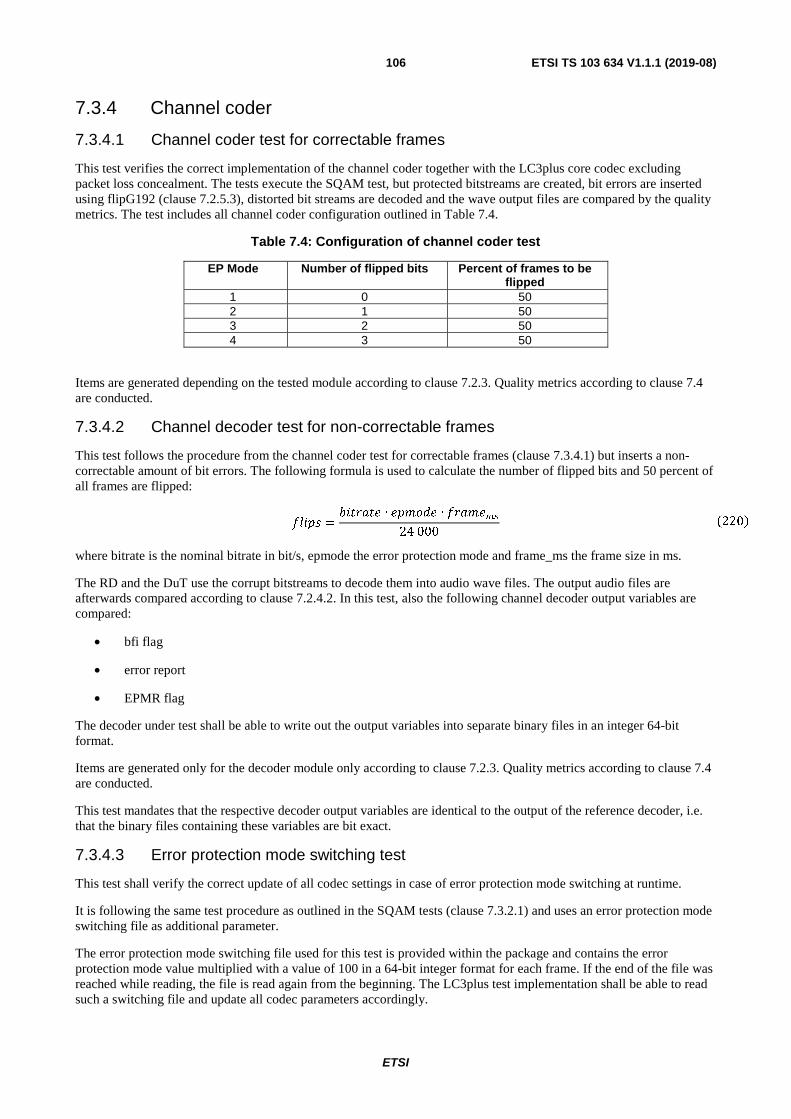
ETSI
ETSI TS 103 634 V1.1.1 (2019-08)106
7.3.4 Channel coder
7.3.4.1 Channel coder test for correctable frames
This test verifies the correct implementation of the channel coder together with the LC3plus core codec excluding packet loss concealment. The tests execute the SQAM test, but protected bitstreams are created, bit errors are inserted using flipG192 (clause 7.2.5.3), distorted bit streams are decoded and the wave output files are compared by the quality metrics. The test includes all channel coder configuration outlined in Table 7.4.
Table 7.4: Configuration of channel coder test
EP Mode Number of flipped bits Percent of frames to be flipped
1 0 50 2 1 50 3 2 50 4 3 50
Items are generated depending on the tested module according to clause 7.2.3. Quality metrics according to clause 7.4 are conducted.
7.3.4.2 Channel decoder test for non-correctable frames
This test follows the procedure from the channel coder test for correctable frames (clause 7.3.4.1) but inserts a non-correctable amount of bit errors. The following formula is used to calculate the number of flipped bits and 50 percent of all frames are flipped:
���� =������ ∙ ������ ∙ �����
24 000�220�
where bitrate is the nominal bitrate in bit/s, epmode the error protection mode and frame_ms the frame size in ms.
The RD and the DuT use the corrupt bitstreams to decode them into audio wave files. The output audio files are afterwards compared according to clause 7.2.4.2. In this test, also the following channel decoder output variables are compared:
• bfi flag
• error report
• EPMR flag
The decoder under test shall be able to write out the output variables into separate binary files in an integer 64-bit format.
Items are generated only for the decoder module only according to clause 7.2.3. Quality metrics according to clause 7.4 are conducted.
This test mandates that the respective decoder output variables are identical to the output of the reference decoder, i.e. that the binary files containing these variables are bit exact.
7.3.4.3 Error protection mode switching test
This test shall verify the correct update of all codec settings in case of error protection mode switching at runtime.
It is following the same test procedure as outlined in the SQAM tests (clause 7.3.2.1) and uses an error protection mode switching file as additional parameter.
The error protection mode switching file used for this test is provided within the package and contains the error protection mode value multiplied with a value of 100 in a 64-bit integer format for each frame. If the end of the file was reached while reading, the file is read again from the beginning. The LC3plus test implementation shall be able to read such a switching file and update all codec parameters accordingly.

ETSI
ETSI TS 103 634 V1.1.1 (2019-08)107
Items are generated depending on the tested module according to clause 7.2.3. Quality metrics according to clause 7.4 are conducted.
7.3.4.4 Combined channel coding test for correctable frames
This test shall verify the correct behaviour of the combined channel coding for a stereo audio input. It follows the same test procedure as outlined in the channel encoder and decoder tests for correctable frames stated in clause 7.3.4.1.
The evaluation of the audio quality within these tests is done separately for each channel, i.e. the output stereo files are split into their individual channels before applying the quality metrics. The worst value out of all channels is then selected for further evaluation.
Items are generated depending on the tested module according to clause 7.2.3. Quality metrics according to clause 7.4 are conducted. The comparison of the channel decoder output variables is applicable only for decoder tests and is not used for encoder and encdec tests.
7.3.4.5 Combined channel coding test for non-correctable frames
This test shall verify the correct behaviour of the combined channel coding for a stereo audio input. It follows the same test procedure as outlined in the channel encoder and decoder tests for non-correctable frames stated in clause 7.3.4.2. The evaluation of the audio quality is performed as outlined in clause 7.3.4.4.
Items are generated depending on the tested module according to clause 7.2.3. Quality metrics according to clause 7.4 are conducted.
7.3.4.6 High-resolution mode test
The high-resolution mode test is for further study.
7.4 Mapping conformance test, module and quality metric
7.4.1 Encoder
Table 7.5 describes the available tests for an LC3plus encoder and the applicable quality metric.
Table 7.5: EuT tests and metrics
Test Name Metric SQAM RMS or ODG Band limitation RMS or ODG Low pass Energy difference Bitrate switching RMS or ODG Bandwidth switching RMS or ODG Channel coder correctable frame RMS or ODG Channel coder error protection mode switching RMS or ODG Combined channel coding correctable frame RMS or ODG
7.4.2 Decoder
Table 7.6 describes the available tests for an LC3plus decoder and the applicable quality metric.

ETSI
ETSI TS 103 634 V1.1.1 (2019-08)108
Table 7.6: DuT tests and metrics
Test Name Metric SQAM RMS Band limitation RMS Bitrate switching RMS Packet loss concealment MLD or RMS Partial concealment MLD or RMS Channel coder correctable frame RMS Channel Coder, Non-correctable frame MLD or RMS Channel coder error protection mode switching RMS Combined channel coding correctable frame RMS Combined channel coding non-correctable frame MLD or RMS
7.4.3 Encoder - decoder (encdec)
Table 7.7 describes the available tests for an LC3plus encdec and the applicable quality metric.
Table 7.7: EuT-DuT tests and metrics
Test Name Metric SQAM RMS or ODG Band limitation RMS or ODG Low pass Energy difference Bitrate switching RMS or ODG Bandwidth switching RMS or ODG Channel coder correctable frame RMS or ODG Channel Coder, Non-correctable frame MLD or RMS Channel coder error protection mode switching RMS or ODG Combined channel coding correctable frame RMS Combined channel coding non-correctable frame MLD or RMS
7.5 Quality metric thresholds The thresholds for each quality metric are outlined in Table 7.8. For each test, the conformance criteria stated in clause 7.6 apply.
Table 7.8: Thresholds for quality metrics
Metric Threshold RMS k = 14 (see note 1) ODG 0,06 (see note 2) Energy difference 70 MLD 4 Binary file (channel coder debug data) Files shall be bitexact NOTE 1: The actual thresholds used within the reference script (RMS in dB
and max. abs. diff.) are derived from k. NOTE 2: An ODG threshold of 0,15 is used for 8 kHz tests.
7.6 Conformance criteria A LC3plus implementation shall pass all required conformance tests to be considered as a conformant implementation. The required codec configurations and conformance test may depend on the application as described in clause 7.7.2. If not stated otherwise, all conformance tests listed in clause 7.4 shall be fulfilled.
A conformance test is considered as passed if all test permutations pass the threshold condition (clause 7.5) with the required quality metric. In case more than one quality metric is allowed, the conformance test shall pass all test permutations for one dedicated quality metric. Mixing the pass/fail results of different quality metrics shall not be allowed. Only one quality metric can be selected in the conformance reference script for each test.

ETSI
ETSI TS 103 634 V1.1.1 (2019-08)109
A conformance test can be considered as failed if at least one of the test conditions of a test permutation does not pass the threshold criteria.
7.7 Codec tests
7.7.1 General LC3plus test
The following lists all possible LC3plus codec parameter configurations:
• Sampling rate in kHz: 8, 16, 24, 32, 48
• Frame size in ms: 2,5, 5, 10
• Bit rate in bytes per frame: 20…400
• Channel coder enabled / disabled
For a full compliant implementation, the conformance criteria in clause 7.5 for all conformance tests listed in clause 7.4 shall be fulfilled.
7.7.2 Applications
The conformance tests depend on the required application. Application test specifications may require additional tests. The application typically defines the codec configuration parameters (clause 7.2.2), i.e. bit rate, sampling rate, etc., and which conformance test groups are required for which modules (clause 7.2.3).
Table 7.9 gives an example which application may require particular conformance tests.
Table 7.9: Example conformance tests for specific applications
LC3plus application
Codec configuration Conformance tests group (see clause 7.3.1) (see note 1)
Sampling rate [Hz]
Frame size [ms]
Bit rate [bytes per
frame]
Core coder Concealment Channel Coder
LC3plus WB Voip 16 000 10 40 Enc, Dec, EncDec
Dec N/A
LC3plus WB Voice DECT
16 000 10 40 Enc, Dec, EncDec
Dec Enc, Dec
LC3plus music DECT
48 000 10 80, 120, 160
(see note 2) Enc, Dec, EncDec
Dec Enc, Dec
LC3plus low delay DECT
32 000 2.5 40, 80 Enc, Dec, EncDec
Dec Enc, Dec (see note 3)
NOTE 1: Some conformance tests are conducted for the modules encoder (enc), decoder (dec) and codec (encdec) separately.
NOTE 2: As LC3plus operates in dual-mono for stereo signals, the conformance tests are applied on mono signals only.
NOTE 3: For some bit rates, the channel coder operates on combined stereo payloads (see clause 7.3.4.4).
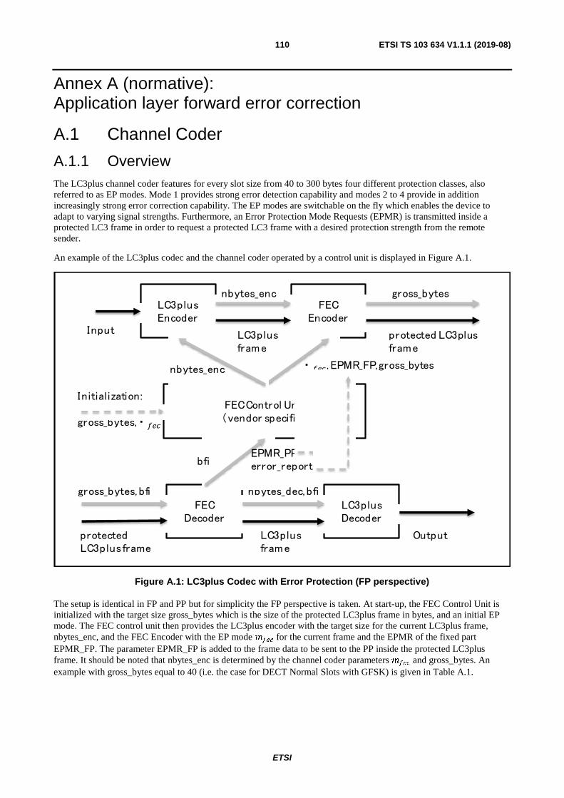
ETSI
ETSI TS 103 634 V1.1.1 (2019-08)110
Annex A (normative): Application layer forward error correction
A.1 Channel Coder
A.1.1 Overview The LC3plus channel coder features for every slot size from 40 to 300 bytes four different protection classes, also referred to as EP modes. Mode 1 provides strong error detection capability and modes 2 to 4 provide in addition increasingly strong error correction capability. The EP modes are switchable on the fly which enables the device to adapt to varying signal strengths. Furthermore, an Error Protection Mode Requests (EPMR) is transmitted inside a protected LC3 frame in order to request a protected LC3 frame with a desired protection strength from the remote sender.
An example of the LC3plus codec and the channel coder operated by a control unit is displayed in Figure A.1.
Figure A.1: LC3plus Codec with Error Protection (FP perspective)
The setup is identical in FP and PP but for simplicity the FP perspective is taken. At start-up, the FEC Control Unit is initialized with the target size gross_bytes which is the size of the protected LC3plus frame in bytes, and an initial EP mode. The FEC control unit then provides the LC3plus encoder with the target size for the current LC3plus frame, nbytes_enc, and the FEC Encoder with the EP mode ��� for the current frame and the EPMR of the fixed part EPMR_FP. The parameter EPMR_FP is added to the frame data to be sent to the PP inside the protected LC3plus frame. It should be noted that nbytes_enc is determined by the channel coder parameters ��� and gross_bytes. An example with gross_bytes equal to 40 (i.e. the case for DECT Normal Slots with GFSK) is given in Table A.1.
FEC
Decoder
LC3plus
Decoder
LC3plus
frame
nbytes_dec,
bfi
protected
LC3plus
frame
gross_bytes,
bfi
Output
FEC
Control
Unit
( vendor specific)
EPMR_PP
error_report
LC3plus
Encoder
FEC
Encoder
LC3plus
frame
nbytes_enc
nbytes_enc � , EPMR_FP,gross_bytes
protected LC3plus
frame
gross_bytes
Input
Initialization:
gross_bytes,
�
bfi
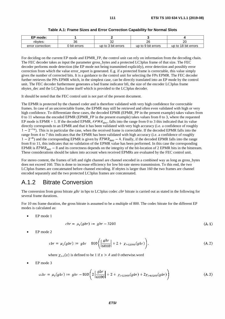
ETSI
ETSI TS 103 634 V1.1.1 (2019-08)111
Table A.1: Frame Sizes and Error Correction Capability for Normal Slots
EP mode: 1 2 3 4 nbytes: 36 32 26 20
error correction: 0 bit errors up to 3 bit errors up to 9 bit errors up to 18 bit errors
For deciding on the current EP mode and EPMR_FP, the control unit can rely on information from the decoding chain. The FEC decoder takes as input the parameter gross_bytes and a protected LC3plus frame of that size. The FEC decoder performs mode detection (the EP mode not being transmitted explicitly), error detection and possibly error correction from which the value error_report is generated. E.g. if a protected frame is correctable, this value simply gives the number of corrected bits. It is a guidance to the control unit for selecting the FPs EPMR. The FEC decoder further retrieves the PPs EPMR which, in the simplest case, can be directly translated into an EP mode by the control unit. The FEC decoder furthermore generates a bad frame indicator bfi, the size of the encoder LC3plus frame nbytes_dec and the LC3plus frame itself which is provided to the LC3plus decoder.
It should be noted that the FEC control unit is not part of the present document.
The EPMR is protected by the channel coder and is therefore validated with very high confidence for correctable frames. In case of an uncorrectable frame, the EPMR may still be retrieved and often even validated with high or very high confidence. To differentiate these cases, the decoded EPMR (EPMR_PP in the present example) takes values from 0 to 11 whereas the encoded EPMR (EPMR_FP in the present example) takes values from 0 to 3, where the requested EP mode is EPMR + 1. If the decoded EPMR, ������� , falls into the range from 0 to 3 this indicated that its value directly corresponds to an EPMR and that it has been validated with very high accuracy (i.e. a confidence of roughly 1 − 2���). This is in particular the case, when the received frame is correctable. If the decoded EPMR falls into the range from 4 to 7 this indicates that the EPMR has been validated with high accuracy (i.e. a confidence of roughly 1 − 2��) and the corresponding EPMR is given by ������� − 4. Finally, if the decoded EPMR falls into the range from 8 to 11, this indicates that no validation of the EPMR value has been performed. In this case the corresponding EPMR is ������� − 8 and its correctness depends on the integrity of the bit-location of 2 EPMR bits in the bitstream. These considerations should be taken into account when received EPMRs are evaluated by the FEC control unit.
For stereo content, the frames of left and right channel are channel encoded in a combined way as long as gross_bytes does not exceed 160. This is done to increase efficiency for low bit-rate stereo transmission. To this end, the two LC3plus frames are concatenated before channel encoding. If nbytes is larger than 160 the two frames are channel encoded separately and the two protected LC3plus frames are concatenated.
A.1.2 Bitrate Conversion The conversion from gross bitrate ��� in bps to LC3plus codec ��� bitrate is carried out as stated in the following for several frame durations.
For 10 ms frame duration, the gross bitrate is assumed to be a multiple of 800. The codec bitrate for the different EP modes is calculated as:
• EP mode 1
��� = ����� ∶= ��� − 3200 A. 1� • EP mode 2
��� = ����� ∶= ��� − 800 � ���6000
� + 2 + ���������� , A. 2� where ���� is defined to be 1 if � > � and 0 otherwise.word
• EP mode 3
���� = ���� ∶= ��� − 800 �2 ���6000
� + 2 + ��������� + 2���������� A. 3�
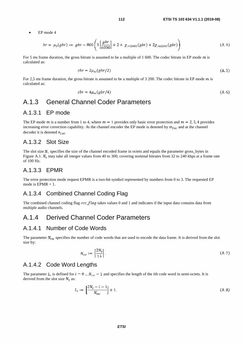
ETSI
ETSI TS 103 634 V1.1.1 (2019-08)112
• EP mode 4
�� = ���� ∶= ��� − 800 �3 ���6000
� + 2 + ��������� + 2���������� A. 4� For 5 ms frame duration, the gross bitrate is assumed to be a multiple of 1 600. The codec bitrate in EP mode � is calculated as:
��� = 2 ���/2� A. 5� For 2,5 ms frame duration, the gross bitrate is assumed to be a multiple of 3 200. The codec bitrate in EP mode � is calculated as:
��� = 4 ���/4� A. 6� A.1.3 General Channel Coder Parameters
A.1.3.1 EP mode
The EP mode � is a number from 1 to 4, where � = 1 provides only basic error protection and � = 2, 3, 4 provides increasing error correction capability. At the channel encoder the EP mode is denoted by ���� and at the channel decoder it is denoted ���� .
A.1.3.2 Slot Size
The slot size �� specifies the size of the channel encoded frame in octets and equals the parameter gross_bytes in Figure A.1. �� may take all integer values from 40 to 300, covering nominal bitrates from 32 to 240 kbps at a frame rate of 100 Hz.
A.1.3.3 EPMR
The error protection mode request EPMR is a two-bit symbol represented by numbers from 0 to 3. The requested EP mode is EPMR + 1.
A.1.3.4 Combined Channel Coding Flag
The combined channel coding flag ���_���� takes values 0 and 1 and indicates if the input data contains data from multiple audio channels.
A.1.4 Derived Channel Coder Parameters
A.1.4.1 Number of Code Words
The parameter ��� specifies the number of code words that are used to encode the data frame. It is derived from the slot size by:
��� ∶= 2��15
� . A. 7� A.1.4.2 Code Word Lengths
The parameter �� is defined for � = 0 … ��� − 1 and specifies the length of the �th code word in semi-octets. It is derived from the slot size �� as:
�� ∶= �2�� − � − 1��� � + 1. A. 8�
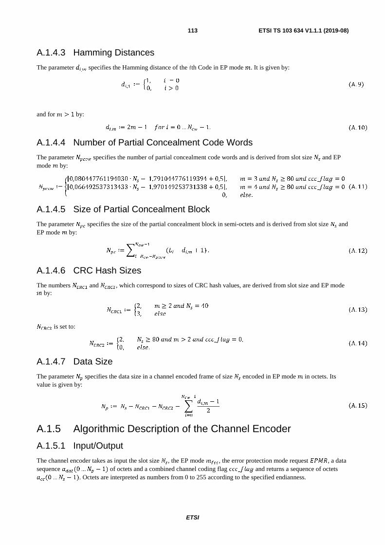
ETSI
ETSI TS 103 634 V1.1.1 (2019-08)113
A.1.4.3 Hamming Distances
The parameter ��, specifies the Hamming distance of the �th Code in EP mode �. It is given by:
��,� ∶= �1, � = 00, � > 0
A. 9�
and for � > 1 by:
��, ∶= 2� − 1 ��� � = 0 … ��� − 1. A. 10�
A.1.4.4 Number of Partial Concealment Code Words
The parameter ����� specifies the number of partial concealment code words and is derived from slot size �� and EP mode � by:
����� ∶= ⌊0,080447761194030 ∙ �� − 1,791044776119394 + 0,5⌋, � = 3 ��� �� ≥ 80 ��� ���_���� = 0⌊0,066492537313433 ∙ �� − 1,970149253731338 + 0,5⌋, � = 4 ��� �� ≥ 80 ��� ���_���� = 00, #�$#.
A. 11�
A.1.4.5 Size of Partial Concealment Block
The parameter ��� specifies the size of the partial concealment block in semi-octets and is derived from slot size �� and EP mode � by:
��� ∶= % (�� − ��, + 1)�����
�����������. A. 12�
A.1.4.6 CRC Hash Sizes
The numbers ����� and �����, which correspond to sizes of CRC hash values, are derived from slot size and EP mode � by:
����� ∶= &2, � ≥ 2 ��� �� = 403, #�$# A. 13�
����� is set to:
����� ∶= &2, �� ≥ 80 ��� � > 2 ��� ���_���� = 0,0, #�$#.
A. 14�
A.1.4.7 Data Size
The parameter �� specifies the data size in a channel encoded frame of size �� encoded in EP mode � in octets. Its value is given by:
�� ∶= �� − ����� − ����� − % ��, − 1
2
�����
���
A. 15�
A.1.5 Algorithmic Description of the Channel Encoder
A.1.5.1 Input/Output
The channel encoder takes as input the slot size ��, the EP mode ����, the error protection mode request ����, a data sequence ����(0 … �� − 1) of octets and a combined channel coding flag ���_���� and returns a sequence of octets ���(0 … �� − 1). Octets are interpreted as numbers from 0 to 255 according to the specified endianness.

ETSI
ETSI TS 103 634 V1.1.1 (2019-08)114
A.1.5.2 Data Pre-Processing
The data sequence is first split into a sequence ��(0 … 2�� − 1) of semi-octets with reversed ordering, where ��(2') holds the upper half of ����(�� − 1 − ') and ��(2' + 1) holds the lower half. In formulas this is:
��2'� ∶= (����)�� − 1 − '*16
+ A. 16�
and:
��2' + 1� ∶= �#�)����)�� − 1 − '*, 16* A. 17�
where �#�(�, ,) denotes the remainder in the long division of � by ,, i.e. the uniquely determined number �, such that 0 ≤ � < |,| and such that � − � is divisible by ,.
Next, CRC hash values are calculated on the bit-expansions of the sequences:
���)0 … 2�� − ��� − 1* ∶= ��(0. . . 2�� − ��� − 1) A. 18�
and:
���)0 … ��� − 1* ∶= ��)2�� − ��� … 2�� − 1* A. 19�
Note that ��� might be zero in which case ��� is the empty sequence. The bit-expansion of a semi-octet sequence �(0 … � − 1) is defined by the sequence �(0 … 4� − 1), where:
�4' + .� ∶= ��/�(�'�)), A. 20�
with ' ranging from 0 to � − 1 and . ranging from 0 to 3 and where ��/� is the function returning the .th bit according to the specified endianness.
The first CRC hash sequence, calculated on an extension of ���, has length 8����� − 2 and the binary generator polynomials are given by:
0���� = 1 + x� + x� + x� + x�� + x�� A. 21�
and:
0���� = 1 + � + �� + �� + �� + ��� + ��� + ��� + ��� + ��� A. 22�
The second CRC hash sequence, calculated on ���, has length 8����� and the binary generator polynomial is given by:
0���� = 1 + � + � + �� + �� + �� + �� + �� + ��� + ��� A. 23�
The CRC hash sequence of length ' on a binary data sequence �(0 … � − 1) for a given binary generator polynomial 0(�) of degree ' is defined as usual to be the binary sequence �(0 … ' − 1) such that the binary polynomial:
�� = %��� �����
���
+ % ������
���
�� � A. 24�
is divisible by 0��.
Let ��� denote the bit-expansion of ��� and let ��� denote the bit-expansion of ���. Then the sequence ���(0 … 8����� − 3) is set to be the hash sequence of length 8����� − 2 calculated on the concatenated sequence:
����!� = 1��/������, ��/������, ���0� … ���)8�� − 4��� − 1*2 . A. 25�
Furthermore, ���(0 … 8����� − 1) is set to be the second hash sequence of length 8����� calculated on ���. Note that ��� is the empty sequence if ����� = 0.
The first pre-processed data sequence ����(0. .8)�� + ����� + �����* − 1) is then defined by:
����0 … 8����� − 3� ∶= ���0 … 8����� − 3�, A. 26�
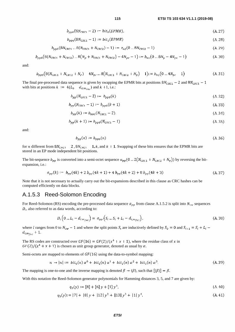
ETSI
ETSI TS 103 634 V1.1.1 (2019-08)115
����8����� − 2� ∶= ��/������, A. 27�
����8����� − 1� ∶= ��/������ A. 28�
����8����� … 8����� + ������ − 1� ∶= ���0 … 8����� − 1� A. 29�
����)8����� + ������ … 8)�� + ����� + �����* − 4��� − 1* ∶= ���)0 … 8�� − 4��� − 1* A. 30�
and:
����)8����� + ����� + �"� − 4��� … 8)����� + ����� + ��* − 1*: = ���)0 … 4��� − 1* A. 31�
The final pre-processed data sequence is given by swapping the EPMR bits at positions 8����� − 2 and 8����� − 1 with bits at positions ' ∶= 4(�� − ��, ���
) and ' +1, i.e.:
�������� − 2� ∶= ����(') A. 32�
�������� − 1� ∶= ����' + 1� A. 33�
���'� ∶= ��������� − 2�. A. 34�
���' + 1� ∶= ����(����� − 1) A. 35�
and:
����� ∶= ����(�) A. 36�
for � different from 8����� − 2 , 8����� − 1, ', and ' + 1. Swapping of these bits ensures that the EPMR bits are stored in an EP mode independent bit positions.
The bit-sequence ��� is converted into a semi-octet sequence ���(0 … 2)����� + ����� + ��*) by reversing the bit-expansion, i.e.:
���'� ∶= ���4'� + 2 ���4' + 1� + 4 ���4' + 2� + 8 ���4' + 3� A. 37�
Note that it is not necessary to actually carry out the bit-expansions described in this clause as CRC hashes can be computed efficiently on data blocks.
A.1.5.3 Reed-Solomon Encoding
For Reed-Solomon (RS) encoding the pre-processed data sequence ��� from clause A.1.5.2 is split into ��� sequences 3� , also referred to as data words, according to:
3� 10 … �� − ��, ���2 = ��� 14� … 4� + �� − ��, ���
2 , A. 38�
where � ranges from 0 to ��� − 1 and where the split points 4� are inductively defined by 4� = 0 and 4� � = 4� + �� −��, ���+ 1.
The RS codes are constructed over 5616� = 56(2)/(�� + � + 1), where the residue class of � in 56(2)/(�� + � + 1) is chosen as unit group generator, denoted as usual by 7.
Semi-octets are mapped to elements of 5616� using the data-to-symbol mapping:
� → 8�9 ∶= ��/��� 7� + ��/��� 7� + ��/��� 7� + ��/�� 7. A. 39�
The mapping is one-to-one and the inverse mapping is denoted : → ⟨:⟩, such that 8⟨:⟩9 = :.
With this notation the Reed-Solomon generator polynomials for Hamming distances 3, 5, and 7 are given by:
=,� ∶= 889 + 869 , + 819 ,�, A. 40�
=�,�: = 879 + 889 , + 8129 ,� + 8139 , + 819 ,�, A. 41�
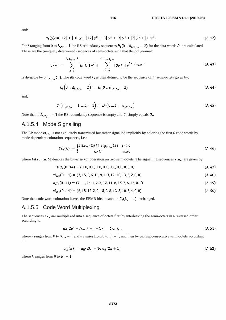
ETSI
ETSI TS 103 634 V1.1.1 (2019-08)116
and:
=�,�: = 8129 + 8109 , + 8129 ,� + 839 , + 899 ,� + 879 ,� + 819 ,� . A. 42�
For � ranging from 0 to ��� − 1 the RS redundancy sequences ��(0 … ��, ���− 2) for the data words 3� are calculated.
These are the (uniquely determined) seqences of semi-octets such that the polynomial:
�,� ∶= % 8��'�9 ,���,����
��
���
+ % 83�'�9 ,� ��,������
#����,����
���
A. 43�
is divisible by =��, ���(,). The �th code word >� is then defined to be the sequence of �� semi-octets given by:
>� 10 … ��, ���− 22 ∶= ��(0 … ��, ���
− 2) A. 44�
and:
>� 1��, ���− 1 … �� − 12 ∶= 3� 10 … �� − ��, ���
2 A. 45�
Note that if ��, ���= 1 the RS redundancy sequence is empty and >� simply equals 3� .
A.1.5.4 Mode Signalling
The EP mode ���� is not explicitely transmitted but rather signalled implicitly by coloring the first 6 code words by mode dependent coloration sequences, i.e.:
>>�'� ∶= ?��/���(>�'�, $�� ���'� � < 6
>�'� #�$#,A. 46�
where ��/���(�, �) denotes the bit-wise xor operation on two semi-octets. The signalling sequences $�� are given by:
$���0. .14� = (0, 0, 0, 0, 0, 0, 0, 0, 0, 0, 0, 0, 0, 0, 0) A. 47�
$���0. .14� = (7, 15, 5, 6, 14, 9, 1, 3, 12, 10, 13, 3, 2, 0, 0) A. 48�
$��0. .14� = (7, 11, 14, 1, 2, 3, 12, 11, 6, 15, 7, 6, 12, 0, 0) A. 49�
$���0. .14� = (6, 15, 12, 2, 9, 15, 2, 8, 12, 3, 10, 5, 4, 0, 0) A. 50�
Note that code word coloration leaves the EPMR bits located in >�(�� − 1) unchanged.
A.1.5.5 Code Word Multiplexing
The sequences >>� are multiplexed into a sequence of octets first by interleaving the semi-octets in a reversed order according to:
��$2�� − ��� ' − � − 1� ∶= >>�'�, A. 51�
where � ranges from 0 to ��� − 1 and ' ranges from 0 to �� − 1, and then by pairing consecutive semi-octets according to:
���'� ∶= ��$2'� + 16 ��$(2' + 1) A. 52�
where ' ranges from 0 to �� − 1.
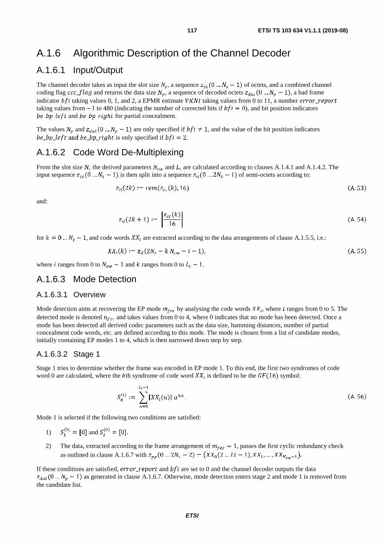
ETSI
ETSI TS 103 634 V1.1.1 (2019-08)117
A.1.6 Algorithmic Description of the Channel Decoder
A.1.6.1 Input/Output
The channel decoder takes as input the slot size ��, a sequence @��(0 … �� − 1) of octets, and a combined channel coding flag ���_���� and returns the data size ��, a sequence of decoded octets @���(0 … �� − 1), a bad frame indicator ��� taking values 0, 1, and 2, a EPMR estimate AB�C taking values from 0 to 11, a number #����_�#0��/ taking values from −1 to 480 (indicating the number of corrected bits if ��� = 0), and bit position indicators �#_�0_�#�/ and �#_�0_���ℎ/ for partial concealment.
The values �� and @���(0 … �� − 1) are only specified if ��� ≠ 1, and the value of the bit position indicators �#_�0_�#�/ and �#_�0_���ℎ/ is only specified if ��� = 2.
A.1.6.2 Code Word De-Multiplexing
From the slot size �� the derived parameters ��� and �� are calculated according to clauses A.1.4.1 and A.1.4.2. The input sequence @��(0 … �� − 1) is then split into a sequence @�$(0 … 2�� − 1) of semi-octets according to:
@�$2'� ∶= �#�(@��'�, 16) A. 53�
and:
@�$2' + 1� ∶= (@��'�16
+ A. 54�
for ' = 0 … �� − 1, and code words DD� are extracted according to the data arrangements of clause A.1.5.5, i.e.:
DD�'� ∶= @�$2�� − ' ��� − � − 1�, A. 55�
where � ranges from 0 to ��� − 1 and ' ranges from 0 to �� − 1.
A.1.6.3 Mode Detection
A.1.6.3.1 Overview
Mode detection aims at recovering the EP mode ���� by analysing the code words DD�, where � ranges from 0 to 5. The detected mode is denoted ���� and takes values from 0 to 4, where 0 indicates that no mode has been detected. Once a mode has been detected all derived codec parameters such as the data size, hamming distances, number of partial concealment code words, etc. are defined according to this mode. The mode is chosen from a list of candidate modes, initially containing EP modes 1 to 4, which is then narrowed down step by step.
A.1.6.3.2 Stage 1
Stage 1 tries to determine whether the frame was encoded in EP mode 1. To this end, the first two syndromes of code word 0 are calculated, where the 'th syndrome of code word DD� is defined to be the 56(16) symbol:
4�%�& ∶= %8DD���9 7��#���
���
. A. 56�
Mode 1 is selected if the following two conditions are satisfied:
1) 4�%�& = [0] and 4�%�& = [0].
2) The data, extracted according to the frame arrangement of ���� = 1, passes the first cyclic redundancy check as outlined in clause A.1.6.7 with @��0 … 2�� − 2� = )DD�2 … �� − 1�, DD�, … , DD�����*.
If these conditions are satisfied, #����_�#0��/ and ��� are set to 0 and the channel decoder outputs the data @���(0 … �� − 1) as generated in clause A.1.6.7. Otherwise, mode detection enters stage 2 and mode 1 is removed from the candidate list.
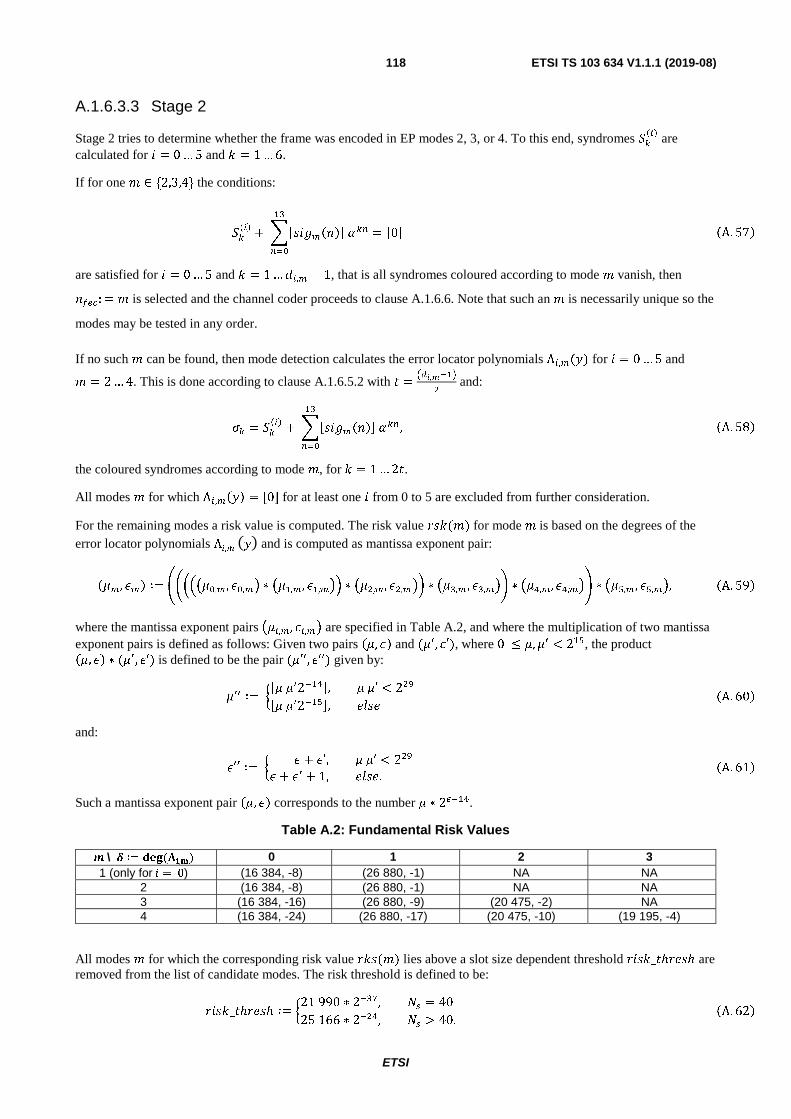
ETSI
ETSI TS 103 634 V1.1.1 (2019-08)118
A.1.6.3.3 Stage 2
Stage 2 tries to determine whether the frame was encoded in EP modes 2, 3, or 4. To this end, syndromes 4�%�& are calculated for � = 0 … 5 and ' = 1 … 6.
If for one � ∈ {2,3,4} the conditions:
4�%�& + %8$�� ��9 7���
���
= 809 A. 57�
are satisfied for � = 0 … 5 and ' = 1 … ��, − 1, that is all syndromes coloured according to mode � vanish, then
����: = � is selected and the channel coder proceeds to clause A.1.6.6. Note that such an � is necessarily unique so the
modes may be tested in any order.
If no such � can be found, then mode detection calculates the error locator polynomials Λ�, (,) for � = 0 … 5 and
� = 2 … 4. This is done according to clause A.1.6.5.2 with / ='��,���(
� and:
E� = 4�%�& + %8$�� ��9 7��,
�
���
A. 58�
the coloured syndromes according to mode �, for ' = 1 … 2/.
All modes � for which Λ� , ,� = [0] for at least one � from 0 to 5 are excluded from further consideration.
For the remaining modes a risk value is computed. The risk value �$'(�) for mode � is based on the degrees of the error locator polynomials Λ),*
�,� and is computed as mantissa exponent pair:
, F � ∶= �GH1)�, , F�, * ∗ )�, , F�, *2 ∗ )�, , F�, *I ∗ ), , F, *J ∗ )�, , F�, *� ∗ )�, , F�, *, A. 59�
where the mantissa exponent pairs )�, , F�, * are specified in Table A.2, and where the multiplication of two mantissa exponent pairs is defined as follows: Given two pairs , F� and (+, F′), where 0 ≤ , + < 2��, the product , F� ∗ (+, F′) is defined to be the pair (++, F′′) given by:
++ ∶= &⌊ +2���⌋, ′ < 2��⌊ +2���⌋, #�$# A. 60�
and:
F′′ ∶= & F + F′, ′ < 2��F + F+ + 1, #�$#.A. 61�
Such a mantissa exponent pair , F� corresponds to the number ∗ 2,���.
Table A.2: Fundamental Risk Values
� \ � ∶= ��� (��,�) 0 1 2 3 1 (only for � = 0) (16 384, -8) (26 880, -1) NA NA
2 (16 384, -8) (26 880, -1) NA NA 3 (16 384, -16) (26 880, -9) (20 475, -2) NA 4 (16 384, -24) (26 880, -17) (20 475, -10) (19 195, -4)
All modes � for which the corresponding risk value �'$(�) lies above a slot size dependent threshold ��$'_/ℎ�#$ℎ are removed from the list of candidate modes. The risk threshold is defined to be:
��$'_/ℎ�#$ℎ ∶= &21 990 ∗ 2��, �� = 40
25 166 ∗ 2���, �� > 40.A. 62�
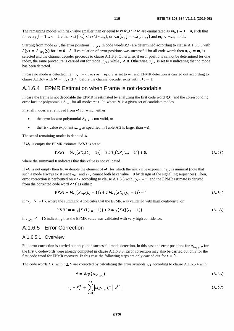
ETSI
ETSI TS 103 634 V1.1.1 (2019-08)119
The remaining modes with risk value smaller than or equal to ��$'_/ℎ�#$ℎ are enumerated as �� , . = 1 … �, such that for every . = 1 … � − 1 either �$')��* < �$'(�� �), or �$')��* = �$')�� �* and �� < �� � holds.
Starting from mode ��, the error positions � �,�,� in code words DD� are determined according to clause A.1.6.5.3 with
Λ,� = Λ�, �,� for � = 0 … 5. If calculation of error positions was successful for all code words then ���� = �� is
selected and the channel decoder proceeds to clause A.1.6.5. Otherwise, if error positions cannot be determined for one index, the same procedure is carried out for mode �� � while . < �. Otherwise, ���� is set to 0 indicating that no mode has been detected.
In case no mode is detected, i.e. ���� = 0 , #����_ �#0��/ is set to −1 and EPMR detection is carried out according to clause A.1.6.4 with � = {1, 2, 3, 4} before the channel decoder exits with ��� = 1.
A.1.6.4 EPMR Estimation when Frame is not decodable
In case the frame is not decodable the EPMR is estimated by analyzing the first code word DD� and the corresponding error locator polynomials Λ�, for all modes � ∈ �, where � is a given set of candidate modes.
First all modes are removed from � for which either:
• the error locator polynomial Λ�, is not valid, or
• the risk value exponent F�, as specified in Table A.2 is larger than −8.
The set of remaining modes is denoted ��.
If �� is empty the EPMR estimate AB�C is set to:
AB�C = ��/�)DD��� − 1�* + 2 ��/�)DD��� − 1�* + 8, A. 63�
where the summand 8 indicates that this value is not validated.
If �� is not empty then let � denote the element of �� for which the risk value exponent F�, is minimal (note that such a mode always exist since F�,� and F�,� cannot both have value −8 by design of the signalling sequences). Then, error correction is performed on DD� according to clause A.1.6.5 with ���� = � and the EPMR estimate is derived from the corrected code word DD�� as either:
AB�C = ��/�)DD���� − 1�* + 2 ��/�)DD���� − 1�* + 4 A. 64�
if F�, > −16, where the summand 4 indicates that the EPMR was validated with high confidence, or:
AB�C = ��/�)DD���� − 1�* + 2 ��/�)DD���� − 1�* A. 65�
if F�, ≤ −16 indicating that the EPMR value was validated with very high confidence.
A.1.6.5 Error Correction
A.1.6.5.1 Overview
Full error correction is carried out only upon successful mode detection. In this case the error positions for �����,�,� for
the first 6 codewords were already computed in clause A.1.6.3.3. Error correction may also be carried out only for the first code word for EPMR recovery. In this case the following steps are only carried out for � = 0.
The code words DD� with � ≤ 5 are corrected by calculating the error symbols K�,� according to clause A.1.6.5.4 with:
� = deg ��,����� �A. 66�
�� = ����� + ���������� ���
��
�
, �A. 67�
ETSI
ETSI TS 103 634 V1.1.1 (2019-08)120
����� being defined as in clause A.1.6.3.3, and:
�� = �����,�,� . �A. 68�
The corrected code words are then defined by:
������� = � �����(������, < ��,� > � = �� ��� ��� ����(�) ���,
�A. 69�
where <∙> is the inverse data-to-symbol mapping specified in clause A.1.5.3.
For the remaining code words with index > 5 error correction is performed by carrying out the usual steps:
1) syndromes are calculated according to:
�� = ��������� ���
�� �
�
�A. 70�
for � = 1 … 2� with � ∶=��,����
�
�.
2) If all syndromes are zero, the code word is presumed error free, and thus the corrected code word ���� is set to ���. 3) Otherwise, the error locator polynomial Λ(y) is calculated according to clause A.1.6.5.2.
4) Upon success (i.e. Λ�y� ≠ [0]), error positions ��, � = 0 … �� − 1 with �� ∶= deg (Λ�y�), are calculated according to clause A.1.6.5.3.
5) Upon success, error symbols ��,� , � = 0 … �� − 1, are calculated according to clause A.1.6.5.4 and error correction is performed according to:
������� = � �����(������, ⟨��,�⟩) � = �� ��� ��� ����(�) ���.
�A. 71�
If error correction fails for an index < "�� − "����, i.e. one of the steps 3, 4 or 5 failed, the bad frame indicator �� is set to 1, �����_��#��� is calculated as specified below and channel decoding is terminated.
For indices ≥ "�� − "���� a sequence $("�� − "���� … "�� − 1) is defined as follows. If error correction fails for an index ≥ "�� − "���� or if the risk value exponent %�,� as specified in Table A.2 is larger than −16 the value $() is set to 0, indicating that the data in code word ��� is not reliable without further validation. If error correction fails for such an index , the corrected code word ���� is nevertheless defined to be ��� but the first bad frame indicator �� is set to 2.
The value of �����_��#��� is determined as follows. If error correction failed for an index < "�� − "���� then let � denote the smalles index for which it failed and set & = '0, . . . , � − 1(. Otherwise let & denote the set of all indices 0 < < "�� for which error correction succeded. The value of �����_��#��� is then calculated as:
�� ��(
��
��∈�
⟨��,�⟩) + ���)⟨��,�⟩* + ���) ⟨��,�⟩* + ���) ⟨��,�⟩* �A. 72�
that is the total number of bits corrected in code words ��� with ∈ &. If "� = 40 the number of bit correction is artificially reduced to increase error detection. If all code words have been corrected successfully the first bad frame indicator is set depending on a mode dependent error threshold ��+�� given by:
��+�� ∶= , 3 � = 1
9 � = 2
18 � = 3
�A. 73�
If �����_��#��� ≤ ��+����� the first bad frame indicator �� is set to 0 and otherwise it is set to 1.
ETSI
ETSI TS 103 634 V1.1.1 (2019-08)121
If "� > 40 and all code words have been corrected successfully, the first bad frame indicator �� is set to 0.
A.1.6.5.2 Calculation of Error Locator Polynomials
The error locator polynomial is calculated from a sequence �� , � = 1 … 2�, of symbols in -.(16), where � is a number from 1 to 3.
If �� = [0] for � = 1 … 2�, the error locator polynomial Λ(y) is set to [1].
Otherwise, the determinants of matrices /� are calculated for � = 1 … �, where:
/� ∶= ����, �A. 74�
/� ∶= ��� ���� ��� , �A. 75�
/� ∶= 0�� �� ���� �� ���� �� ��1 �A. 76�
And
det�/�� = ��, �A. 77�
det�/�� = ���� + ���, �A. 78�
det�/�� = ������ + ����� + ����� + ���. �A. 79�
If all determinants are [0] for � = 1 … � the error locator polynomial Λ�2� is set to [0], which is a non-valid error locator polynomial in the sense of clause A.1.6.5.3.
Otherwise, take 3 to be the largest index from 1 to t such that det�/�� ≠ 0. Then the coefficients of the error locator polynomial are computed as:
04�⋮4�1 ∶= /�
� 0����⋮��� 1 �A. 80�
where the inverse matrices are given by:
/� � ∶= ��� ��, �A. 81�
/� � ∶= det�/�� � ��� ���� ��� , �A. 82�
/� � ∶= det�/�� � 5 ���� + ��� ���� + ���� ���� + ������� + ���� ���� + ��� ���� + �������� + ��� ���� + ���� ���� + ��� 6 . �A. 83�
If 4� = [0], the error locator polynomial is set to �0�. Otherwise, if 3 = �, the error locator polynomial is set to:
Λ�2� ∶= [1] + 4� 2 + … + 4� 2� �A. 84�
and if 3 < � it is further tested whether:
� ������ 4� ��� = ��������
��
�A. 85�
holds for � = 0. .2�� − 3� − 1. If all these equalities hold, then the error locator polynomial is set to:
Λ�2� ∶= [1] + 4� 2 + … + 4� 2� �A. 86�
Otherwise, it is set to [0].
ETSI
ETSI TS 103 634 V1.1.1 (2019-08)122
A.1.6.5.3 Calculation of Error Positions
Error positions are calculated from the error locator polynomial:
Λ�2� ∶= �1� + 4� 2 + … + 4� 2� . �A. 87�
The error locator polynomial is said to be valid, if it admits a representation:
Λ�2� = 7�2 + � ���, where 0 ≤ �� < 8� and
� �
�
�� ≠ �� for � ≠ � �A. 88�
in which case the error positions are given by �� for � = 0 … � − 1. Otherwise, the list of error positions is empty.
The values �� can be determined by testing Λ�� �� = 0 for � = 0 … 8� − 1. Alternatively, tabulation of error locations indexed by 4� is possible and might be considerably faster.
A.1.6.5.4 Calculation of Error Symbols
Error symbols are calculated from syndromes ��, … , �� and error positions �, … , �� � by solving the linear system:
9���, … , �� �� 0 �⋮�� �1 = 0��
⋮��1 �A. 89�
over -.�16�, where 9���, … , �� �� are the Vandermonde matrices:
9���� ∶= ����� �A. 90�
9���, ��� ∶= � ��� ������� ����� , �A. 91�
and:
9���, ��, ��� ∶= 0 ��� ��� ������ ���� ������� ���� ���
1 . �A. 92�
The matrix inverses are given by:
9� ���� = �� ��� �A. 93�
9� ���, ��� = det)9���, ���* � ����� ������� ���� , �A. 94�
and:
9� ���, ��, ��� = det�9���, �� , ��� � � 0������� + ������� ������ + ������ ������ + ������������� + ������� ������ + ������ ������ + �������������� + �������� ������� + ������� ������� + �������
1 �A. 95�
with:
det(9�( �, ��)) = ������� + ������� �A. 96�
and:
det�9���, ��, ��� � = ���������� + ���������� + ���������� + ���������� + ���������� + ���������� . �A. 97�
A.1.6.6 De-Colouration and RS Decoding
De-coloration according to the detected EP mode ���� is done by applying the corresponding signalling sequence from clause A.1.5.4, giving rise to de-colourated code words:
����� ∶= :�����(���� ���, ��������) < 6,������� ���.�A. 98�
ETSI
ETSI TS 103 634 V1.1.1 (2019-08)123
Then, redundancy decoding is applied according to mode ���� producing the data words:
;� �0 … 8� − ��,����� ∶= �� ���,���� − 1. . . 8� − 1� �A. 99�
which are combined into the data sequence <��(0 … "� − 1), with "� as specified in clause A.1.4.7 with � = ����, according to:
<�� ��� … �� + 8� − ��,����� ∶= ;�(0. . . 8� − ��,����) �A. 100�
for = 0 … "�� − 1, where the split points �� are defined as in clause A.1.5.3. This yields a sequence of length 2("� + "� �� + "� ��). After RS redundancy decoding the FEC decoder proceeds to clause A.1.6.7 Data Post-Processing.
A.1.6.7 Data Post-Processing
Data post-processing consists of hash removal and validation, and EPMR extraction. The sequence <�� from clause A.1.6.7 is expanded into the corresponding bit sequence 2�� from which the sequence 2�� is derived by reversing the bit swap from clause A.1.5.2, i.e. swapping bits at positions 8"� �� − 2 and � ∶= 4(8 − �,����
) and
bits at positions 8"� �� − 2 and � +1.
The sequence 2�� is then split into sequences ��, ��, 2���!� , and 2��, corresponding to sequences ���, ���, ����!� , and ��� from clause A.1.5.2, given by:
���0 … 8"� �� − 3� ∶= 2���0 … 8"� �� − 3�, �A. 101�
���0 … 8"� �� − 1� ∶= 2���8"� �� … 8�"� �� + "� ��� − 1�, �A. 102�
2���!��0 … 1� ∶= 2���8"� �� − 3 … 8"� �� − 1�, �A. 103�
2���!�)2 … 8"� − 4"�� + 1* ∶= 2��(8�"� �� + "� ��� … 8�"� �� + "� �� + ""� − 4"�� − 1 �A. 104�
and:
2��)0 … 4"�� − 1* ∶= 2��(8�"� �� + "� �� + ""� − 4"�� … 8)"� �� + "� �� + "�* �A. 105�
The two cyclic redundancy checks (CRC) are carried out on 2���!� and 2�� by re-calculating the hash sequences specified in clause A.1.5.2.
If the calculated 8"� �� − 2 bit redundancy sequence for 2���!� specified in clause A.1.5.2 does not match �� the bad frame indicator �� is set to 1 and the EPMR is estimated according to clause A.1.6.4 with / = =����>. Otherwise, the EPMR estimate is set to:
?@"& = 2���!��0� + 2 2���!��1�. �A. 106�
If the first CRC is passed and if �� ≠ 2, the second CRC is carried out calculating the 8"� �� hash sequence for 2�� as specified in clause A.1.5.2. If the result does not match the sequence �� the bad frame indicator �� is set to 2, indicating the loss of partial concealment data. If the first CRC is passed and �� = 2 then �� is set to 2 without carrying out the second CRC.
If both CRCs are passed, the bad frame indicator �� is set to 0, indicating that the decoded data is valid.
If ��= 2, the position indicators ��_�#_���� and ��_�#_��ℎ� representing the left and right border of the potentially corrupted bits in the partial concealment block are determined from the sequence $("�� − "���� … "�� − 1) from clause A.1.6.5 in the following way.
If one of the two following conditions is true, then ��_�#_���� is set to 0 and ��_�#_��ℎ� is set to 4"�� − 1.
1) $�� = 0 for "�� − "���� ≤ < "�� (no trusted code words exist)
2) $�� = 1 for "�� − "���� ≤ < "�� (all code words are trusted but errors have been detected)
ETSI
ETSI TS 103 634 V1.1.1 (2019-08)124
Otherwise, the position indicators are calculated as follows. If $�"�� − 1� = 0, then ��_�#_���� is set to 0. Otherwise, there exists a maximal index such that $�� = 1 for ≤ < "�� and ��_�#_���� is calculated as:
��#���� = 4 � �8� − ��,���� + 1�$�� �
���
. �A. 107�
Analogously, there exists a minimal index � such that "�� − "���� ≤ � < "�� and $��� = 0, and ��_�#_��ℎ� is calculated as:
��#� ���� = 4 � �8� − ��,���� + 1� − 1
$�� �
���
. �A. 108�
If �� ≠ 1 the output data <�%� is generated by reversing the pre-processing steps from clause A.1.5.2 by setting:
2��)0 … 8"� − 4"�� − 1* ∶= 2���!�)2 … 8"� − 4"�� + 1*, �A. 109�
<����� = 2���4�� + 2 2���4� + 1� + 4 2���4� + 2� + 8 2��(4� + 2) �A. 110�
for � = 0 … 2"� − "�� − 1,
<����� = 2���4�� + 2 2���4� + 1� + 4 2���4� + 2� + 8 2��(4� + 2) �A. 111�
for � = 0 … "�� − 1,
<�)0 … 2"� − "�� − 1* ∶= <�� �A. 112�
<�)2"� − "�� … 2"� − 1* ∶= <�� �A. 113�
and:
<�%���� ∶= <�)2"� − 2� − 1* + 16 <�(2"� − 2� − 2) �A. 114�
for � = 0 … "� − 1.
A.1.7 Padding bytes Padding bytes can be detected as the special decoder mode PADDING described in clause 5.4.2.4. The difference for operating with enabled channel coder is that the padding signalling elements (see Table 5.20) are read from the right side of the LC3plus frame. The additional number of bytes to be skipped as described in the padding length bits are located at the left side of the LC3plus frame in order to optimize the bitstream layout for partial concealment described in clause A.1.8.3.
The decoding procedure complies of a regular channel decoding step. Then when all potential PADDING signal 16-bit code words are detected, the number of padding signals is counted as nsig_pad and the number of padded bytes in the code words is counted as nbytes_padd. The left sided and right sided padding bytes are to be removed and the codec parameters need to be updated according to the real bit rate, see clause 5.7.
If padding is detected the output parameters of the LC3 channel coder are updated according to the following pseudo-code:
Np = Np – 2*nsig_pad – nbytes_pad; Npc = max(Npc – 2*nbytes_sig, 0); if (bfi == 2) { if (be_bp_right < 8*nbytes_pad) { bfi = 0; } else { be_bp_left = max(be_bp_left – 8*nbytes_pad, 0); be_bp_right = be_bp_right – 8*nbytes_pad; }
ETSI
ETSI TS 103 634 V1.1.1 (2019-08)125
}
If padding removal results in a payload size smaller than 20 bytes, i.e. the minimal LC3 payload size, the bad frame indicator is set to 1.
A.1.8 Bit error Concealment
A.1.8.1 Reorder Bitstream
Before the channel coder is applied at encoder side, the bitstream is reordered such that preferably the coding data corresponding to the highest spectral coefficients including the residual signal are in front of the bitstream. At decoder side, the bitstream is read in a different way to repeal the reordering mechanism.
At encoder side, the bitstream bs is rearranged as follows:
bs_rearranged(k) = A bs_enc(b_left + �) , 0 ≤ � < block_size
bs_enc(� − block_size) , block_size ≤ � < b_left + block_sizebs_enc(�) , b_left + block_size ≤ k < len
�A. 115�
where:
len = 8 ∙ ��2�� �A. 116�
and:
block_size = 8 B"��2
C �A. 117�
and "�� calculated in clause A.1.4.5 subject to the changes in clause A.1.7 and b_left is the byte position at the left side where the last block_size bits fit exactly in the bitstream, this means that the partial concealment block is [b_left:b_left+block_size-1].
The rearrangement of the bitstream bs_rearranged at decoder side is done by initializing the arithmetic decoder byte position bp = block_size instead of 0 as done in clause 5.4.2.2. The border b_left at decoder side is determined as:
�_���� = �#_�� , � �#++ == �#_�� �� �# == �#_��--. �A. 118�
If bp++ == b_left, then bp = 0; if bp_side-- == b_left -1, then bp_side = (block_size/8)-1.
If the arithmetic decoder triggers an unexpected bit error in the partial concealment block, meaning outside the range [��_�#_����: ��_�#_��ℎ�], then the lowest MDCT bin which cannot be decoded, �#�, is set to the highest frequency, which can be decoded outside the partial concealment block.
A.1.8.2 Bit error Concealment trigger
If only part of the residual is missing, for example ��_�#_���� and ��_�#_��ℎ� only affect residual bits, then the bfi flag is set to zero and the residual block is skipped, before decoding the frame as a regular frame.
If the previous frame was concealed with packet loss concealment, then the current frame will also be concealed with packet loss concealment of clause 5.6.3. Otherwise, if �#� is the lowest MDCT bin which cannot be decoded and �#� < 4"��, then the decoder shall also apply packet loss concealment for the following five events:
a) If there are uncorrectable bit errors in the bitstream, except the partial concealment code block
b) If the stability factor D according to equation (157) is lower than 0,5
c) If D ≥ 0,5 and pitch_present = 1 as described in clause 5.4.2.3 and �#� < E800$�
��F
d) If D ≥ 0,5 and pitch_present = 1 and �#� < peak_detector(�G�&�' , "(), where �G�&�' is the shaped spectrum of the last non-PLC frame and:
function [�����] = pc_peak_detector(������, ��) block_size = 3; thresh1 = 8; fac = 0.3;
ETSI
ETSI TS 103 634 V1.1.1 (2019-08)126
mean_block_nrg = mean(������.^2); maxPeak = 0; ����� = 0; if abs(������(0)) > abs(������(1))
block_cent = sum(������(0:1).^2); if block_cent/block_size > thresh1*mean_block_nrg cur_max = max(abs(������(0:1)));
next_max = max(abs(������(2:2+block_size-1))); if cur_max > next_max maxPeak = block_cent; ����� = 1; for k = 0:block_size-1 if abs(������(k+1)) >= abs(������(k)) && abs(������(k+1)) >= abs(������(k+2))
block_cent = sum(������(k:k+block_size-1).^2); if block_cent/block_size > thresh1*mean_block_nrg cur_max = max(abs(������(k:k+block_size-1))); prev_max = 0; for j = k-block_size:k-1 if j > 0 prev_max = max(abs(������(j)), prev_max);
next_max = max(abs(������(k+block_size:k+2*block_size-1))); if cur_max >= prev_max && cur_max > next_max if block_cent > fac*maxPeak ����� = k+block_size-1; if block_cent >= maxPeak maxPeak = block_cent; for k = block_size.. ��-(2*block_size) if abs(������(k+1)) >= abs(������(k)) && abs(������(k+1)) >= abs(������(k+2))
block_cent = sum(������(k:k+block_size-1).^2); if block_cent/block_size > thresh1*mean_block_nrg cur_max = max(abs(������(k:k+block_size-1)));
prev_max = max(abs(������(k-block_size:k-1)));
next_max = max(abs(������(k+block_size:k+2*block_size-1))); if cur_max >= prev_max && cur_max > next_max if block_cent > fac*maxPeak ����� = k+block_size-1; if block_cent >= maxPeak maxPeak = block_cent;
e) If D ≥ 0.5 and pitch_present = 0 and:
� �),�*H���� ��� �
�
< 0.3 � �),�*H���� $� �
�
�A. 119�
where �),�*H��� is the quantized spectrum of the last non-PLC frame of clause 5.4.2.8.
If the previous frame was not concealed with packet loss concealment and either none of the five events triggers or �#� ≥ 4"��, partial concealment of clause A.1.8.3 will be applied.
A.1.8.3 Partial Concealment
The partial concealment is a method to conceal the missing spectral lines, which for example are not available due to non-correctable bit errors in the partial concealment code block encapsulated by ��_�#_���� and ��_�#_��ℎ� as described in clause A.1.6.7, while decoding the rest of the payload as usual. Figure A.2 gives a decoder overview including the partial concealment processing blocks marked in green and the update steps marked in red which have to be done in every frame expect for frames which are concealed with PLC.
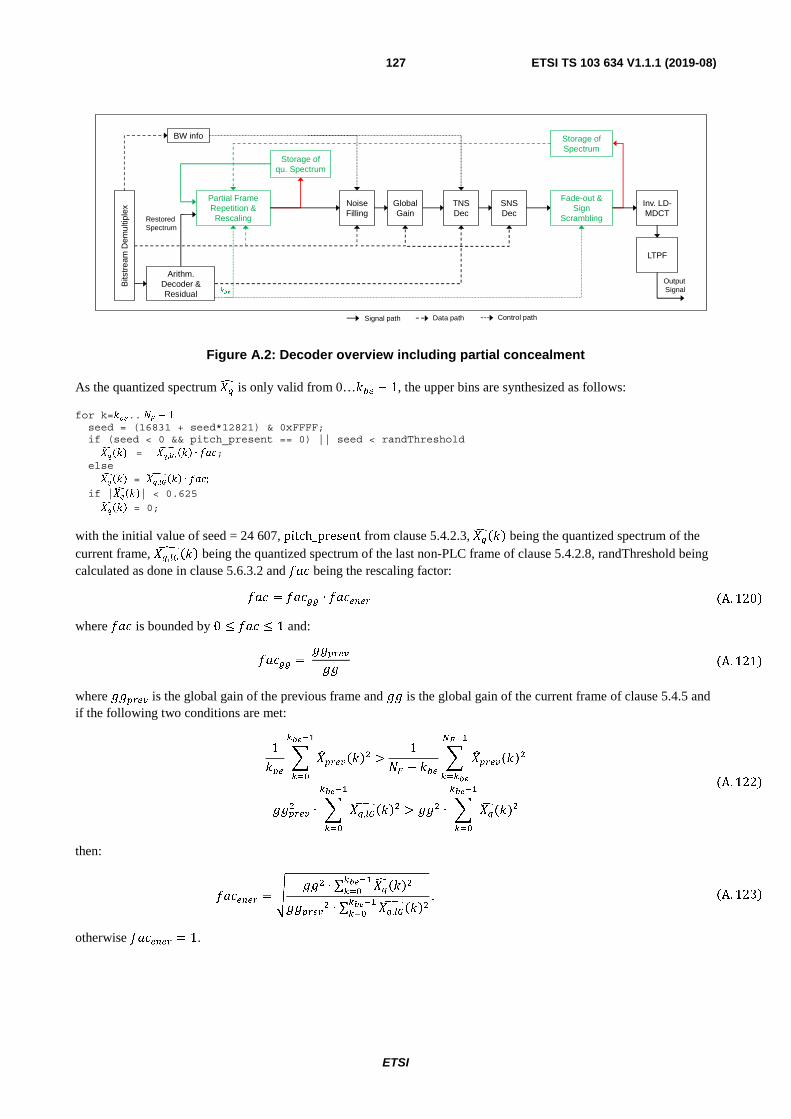
ETSI
ETSI TS 103 634 V1.1.1 (2019-08)127
Figure A.2: Decoder overview including partial concealment
As the quantized spectrum �)I is only valid from 0…�#� − 1, the upper bins are synthesized as follows:
for k=���.. �� − 1 seed = (16831 + seed*12821) & 0xFFFF; if (seed < 0 && pitch_present == 0) || seed < randThreshold ��(�) = −�,�
���� ∙ �; else ����� = �,�
���� ∙ �;
if |�����| < 0.625
����� = 0;
with the initial value of seed = 24 607, pitch_present from clause 5.4.2.3, �)I��� being the quantized spectrum of the current frame, �),�*
H��� being the quantized spectrum of the last non-PLC frame of clause 5.4.2.8, randThreshold being calculated as done in clause 5.6.3.2 and �+J being the rescaling factor:
�+J = �+J++ ∙ �+J���& �A. 120�
where �+J is bounded by 0 ≤ �+J ≤ 1 and:
�+J++ = ���&�'�� �A. 121�
where ���&�' is the global gain of the previous frame and �� is the global gain of the current frame of clause 5.4.5 and if the following two conditions are met:
1�#� � �G�&�'������� �
�
>1"( − �#� � �G�&�'����$� �
����
���&�'� ∙ � �),�*H������� �
�
> ��� ∙ � �)I(�)�
��� �
�
�A. 122�
then:
�+J���& = K ��� ∙ ∑ �)I������� �
����&�'� ∙ ∑ �),�*H������� �
�
. �A. 123�
otherwise �+J���& = 1.
Bits
trea
mD
emul
tiple
x Inv. LD-MDCT
OutputSignal
SNS Dec
GlobalGain
Arithm. Decoder & Residual
Noise Filling
LTPF
TNS Dec
Restored Spectrum
BW info
Signal path Data path Control path
Partial Frame Repetition &Rescaling
Storage of Spectrum
���
Storage of qu. Spectrum
Fade-out &Sign
Scrambling
ETSI
ETSI TS 103 634 V1.1.1 (2019-08)128
Afterwards, the residual decoding in clause 5.4.3 is skipped. Other than that, the frame is processed and handled as a regular good frame, meaning that the blocks noise filling, global gain, temporal noise shaping and spectral noise shaping are applied to form the intermediate spectrum ��′(�) right before the IMDCT, see Figure A.2. To form the reconstructed spectrum ��(�), the intermediate spectrum ��′(�) is damped adaptively based on the two damping factors:
����� = �0,8 + 0,2 ∙ �
, ��� �� = 2,50,8 + 0,2 ∙ �
, ��� �� = 5
0,8 + 0,2 ∙ , ��ℎ������ �A. 124� and:
����� = �0,3 + 0,2 ∙ �
, ��� �� = 2,50,3 + 0,2 ∙ �
, ��� �� = 5
0,3 + 0,2 ∙ , ��ℎ������ �A. 125�
where is the stability factor according to equation (157), but between ��������� and �������. The corresponding cumulative attenuation factors cum_fading_slow� and cum_fading_fast� are derived as follows:
cum_fading_slow� = cum_fading_slow��� ∙ slow� �A. 126� and:
cum_fading_fast� = cum_fading_slow��� ∙ fast� �A. 127� where cum_fading_slow��� and cum_fading_fast��� are the cumulative attenuation factors of the previous frame or 1 if nbLostFrames = 1, where nbLostFrames is the number of consecutive frames which are concealed with partial concealment.
Finally, the damping is processed as follows:
ad_ThreshFac_start = 10; ad_ThreshFac_end = 1.2; ad_threshFac = (ad_ThreshFac_start - ad_ThreshFac_end) * linFuncStartStop + ad_ThreshFac_end;
frame_energy = mean(��′(�)(���.. �� − 1).^2); energThreshold = ad_threshFac * frame_energy;
for k=���.. �� − 1 if (��′(�)^2) < energThreshold m = cum_fading_slow; n = 0; else m = cum_fading_fast; n = (cum_fading_slow-cum_fading_fast) * sqrt(energThreshold) * sign(��′(�)); end ��(�) = m * ��′(�) + n; end
to form the spectrum ��(�) for clause 5.4.8.
A.2 Redundancy frames
A.2.1 Overview A packet-based application layer forward error correction algorithm can be implemented with LC3plus as well. In [i.6], this mechanism is described as media specific FEC. This means a packet contains a primary encoded LC3plus frame and a secondary LC3plus frame which is delayed in time by an offset of t packets.
As packet loss usually coincides with high jitter, a jitter buffer manager can compensate for the high jitter and may forward the secondary LC3plus frame in order to compensate the missing primary frame. Primary and secondary frame might be identical in terms of configuration and bitrate or the secondary frame might be of lower bit rate and lower quality.
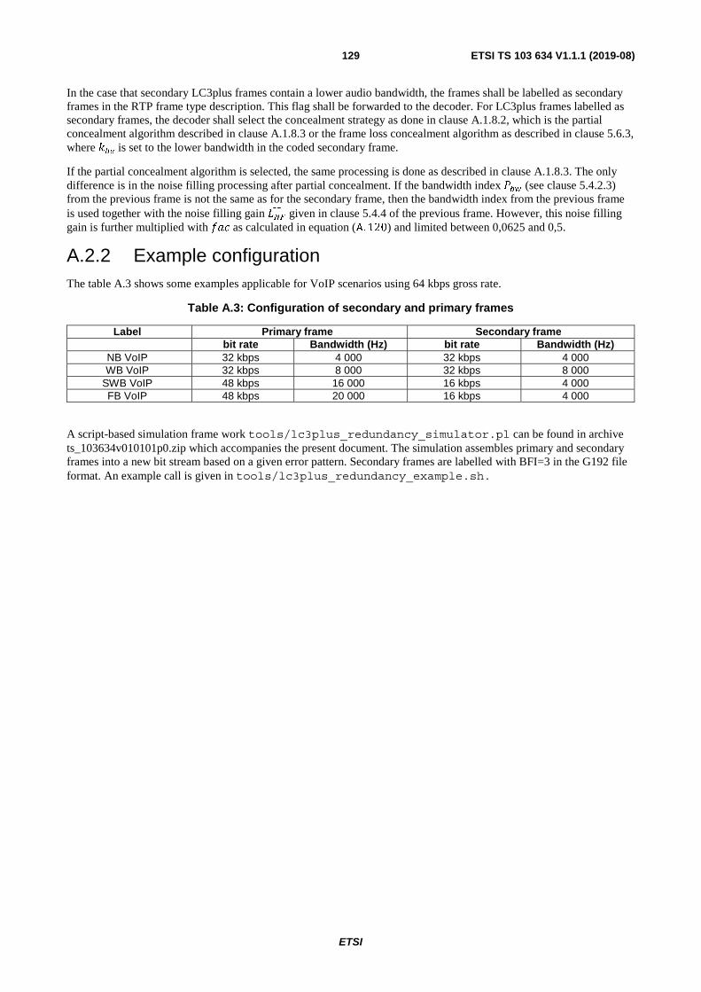
ETSI
ETSI TS 103 634 V1.1.1 (2019-08)129
In the case that secondary LC3plus frames contain a lower audio bandwidth, the frames shall be labelled as secondary frames in the RTP frame type description. This flag shall be forwarded to the decoder. For LC3plus frames labelled as secondary frames, the decoder shall select the concealment strategy as done in clause A.1.8.2, which is the partial concealment algorithm described in clause A.1.8.3 or the frame loss concealment algorithm as described in clause 5.6.3, where ��� is set to the lower bandwidth in the coded secondary frame.
If the partial concealment algorithm is selected, the same processing is done as described in clause A.1.8.3. The only difference is in the noise filling processing after partial concealment. If the bandwidth index �� (see clause 5.4.2.3) from the previous frame is not the same as for the secondary frame, then the bandwidth index from the previous frame is used together with the noise filling gain ��� given in clause 5.4.4 of the previous frame. However, this noise filling gain is further multiplied with ��� as calculated in equation (A. 120) and limited between 0,0625 and 0,5.
A.2.2 Example configuration The table A.3 shows some examples applicable for VoIP scenarios using 64 kbps gross rate.
Table A.3: Configuration of secondary and primary frames
Label Primary frame Secondary frame bit rate Bandwidth (Hz) bit rate Bandwidth (Hz)
NB VoIP 32 kbps 4 000 32 kbps 4 000 WB VoIP 32 kbps 8 000 32 kbps 8 000
SWB VoIP 48 kbps 16 000 16 kbps 4 000 FB VoIP 48 kbps 20 000 16 kbps 4 000
A script-based simulation frame work tools/lc3plus_redundancy_simulator.pl can be found in archive ts_103634v010101p0.zip which accompanies the present document. The simulation assembles primary and secondary frames into a new bit stream based on a given error pattern. Secondary frames are labelled with BFI=3 in the G192 file format. An example call is given in tools/lc3plus_redundancy_example.sh.
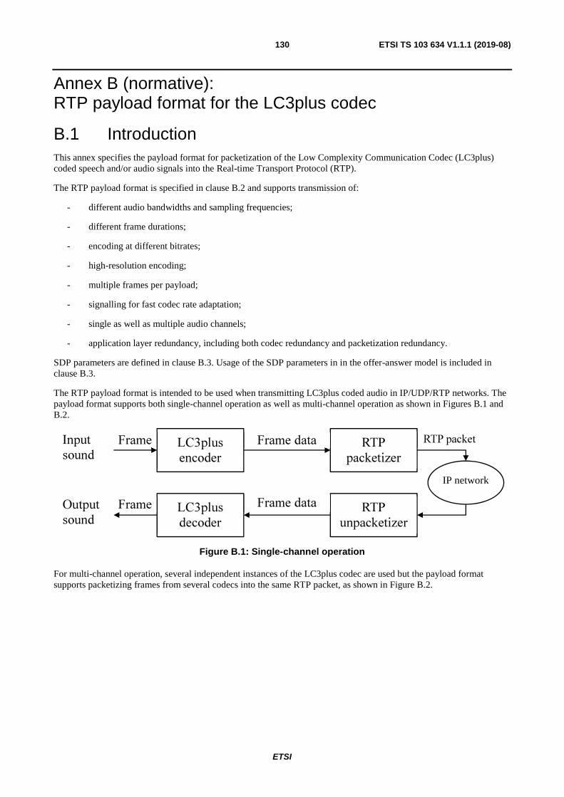
ETSI
ETSI TS 103 634 V1.1.1 (2019-08)130
Annex B (normative): RTP payload format for the LC3plus codec
B.1 Introduction This annex specifies the payload format for packetization of the Low Complexity Communication Codec (LC3plus) coded speech and/or audio signals into the Real-time Transport Protocol (RTP).
The RTP payload format is specified in clause B.2 and supports transmission of:
- different audio bandwidths and sampling frequencies;
- different frame durations;
- encoding at different bitrates;
- high-resolution encoding;
- multiple frames per payload;
- signalling for fast codec rate adaptation;
- single as well as multiple audio channels;
- application layer redundancy, including both codec redundancy and packetization redundancy.
SDP parameters are defined in clause B.3. Usage of the SDP parameters in in the offer-answer model is included in clause B.3.
The RTP payload format is intended to be used when transmitting LC3plus coded audio in IP/UDP/RTP networks. The payload format supports both single-channel operation as well as multi-channel operation as shown in Figures B.1 and B.2.
Figure B.1: Single-channel operation
For multi-channel operation, several independent instances of the LC3plus codec are used but the payload format supports packetizing frames from several codecs into the same RTP packet, as shown in Figure B.2.
LC3plus encoder
Input
sound Frame RTP
packetizer
LC3plus decoder
RTP unpacketizer
Frame data
Output
sound Frame Frame data
IP network
RTP packet
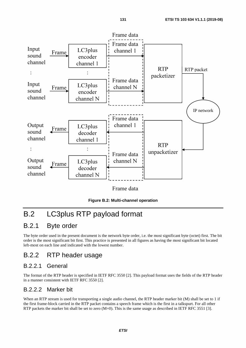
ETSI
ETSI TS 103 634 V1.1.1 (2019-08)131
Figure B.2: Multi-channel operation
B.2 LC3plus RTP payload format
B.2.1 Byte order The byte order used in the present document is the network byte order, i.e. the most significant byte (octet) first. The bit order is the most significant bit first. This practice is presented in all figures as having the most significant bit located left-most on each line and indicated with the lowest number.
B.2.2 RTP header usage
B.2.2.1 General
The format of the RTP header is specified in IETF RFC 3550 [2]. This payload format uses the fields of the RTP header in a manner consistent with IETF RFC 3550 [2].
B.2.2.2 Marker bit
When an RTP stream is used for transporting a single audio channel, the RTP header marker bit (M) shall be set to 1 if the first frame-block carried in the RTP packet contains a speech frame which is the first in a talkspurt. For all other RTP packets the marker bit shall be set to zero (M=0). This is the same usage as described in IETF RFC 3551 [3].
LC3plus encoder
channel 1
Input
sound channel
Frame
RTP packetizer
LC3plus decoder
channel 1 RTP
unpacketizer
Frame data channel 1
Output
sound channel
Frame
Frame data channel 1
IP network
RTP packet
LC3plus encoder
channel N
Input
sound channel
Frame
Frame data channel N
LC3plus decoder
channel N
Output
sound channel
Frame
Frame data channel N
Frame data
Frame data
:
:
:
:
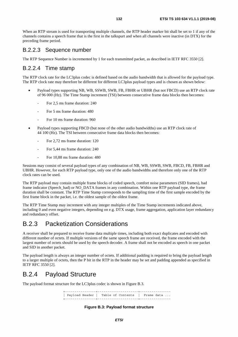
ETSI
ETSI TS 103 634 V1.1.1 (2019-08)132
When an RTP stream is used for transporting multiple channels, the RTP header marker bit shall be set to 1 if any of the channels contains a speech frame that is the first in the talkspurt and when all channels were inactive (in DTX) for the preceding frame period.
B.2.2.3 Sequence number
The RTP Sequence Number is incremented by 1 for each transmitted packet, as described in IETF RFC 3550 [2].
B.2.2.4 Time stamp
The RTP clock rate for the LC3plus codec is defined based on the audio bandwidth that is allowed for the payload type. The RTP clock rate may therefore be different for different LC3plus payload types and is chosen as shown below:
• Payload types supporting NB, WB, SSWB, SWB, FB, FBHR or UBHR (but not FBCD) use an RTP clock rate of 96 000 (Hz). The Time Stamp increment (TSI) between consecutive frame data blocks then becomes:
- For 2,5 ms frame duration: 240
- For 5 ms frame duration: 480
- For 10 ms frame duration: 960
• Payload types supporting FBCD (but none of the other audio bandwidths) use an RTP clock rate of 44 100 (Hz). The TSI between consecutive frame data blocks then becomes:
- For 2,72 ms frame duration: 120
- For 5,44 ms frame duration: 240
- For 10,88 ms frame duration: 480
Sessions may consist of several payload types of any combination of NB, WB, SSWB, SWB, FBCD, FB, FBHR and UBHR. However, for each RTP payload type, only one of the audio bandwidths and therefore only one of the RTP clock rates can be used.
The RTP payload may contain multiple frame blocks of coded speech, comfort noise parameters (SID frames), bad frame indicator (Speech_bad) or NO_DATA frames in any combination. Within one RTP payload type, the frame duration shall be constant. The RTP Time Stamp corresponds to the sampling time of the first sample encoded by the first frame block in the packet, i.e. the oldest sample of the oldest frame.
The RTP Time Stamp may increment with any integer multiples of the Time Stamp increments indicated above, including 0 and even negative integers, depending on e.g. DTX usage, frame aggregation, application layer redundancy and redundancy offset.
B.2.3 Packetization Considerations A receiver shall be prepared to receive frame data multiple times, including both exact duplicates and encoded with different number of octets. If multiple versions of the same speech frame are received, the frame encoded with the largest number of octets should be used by the speech decoder. A frame shall not be encoded as speech in one packet and SID in another packet.
The payload length is always an integer number of octets. If additional padding is required to bring the payload length to a larger multiple of octets, then the P bit in the RTP in the header may be set and padding appended as specified in IETF RFC 3550 [2].
B.2.4 Payload Structure The payload format structure for the LC3plus codec is shown in Figure B.3.
+----------------+---------------------+---------------- | Payload Header | Table of Contents | Frame data ... +----------------+---------------------+----------------
Figure B.3: Payload format structure
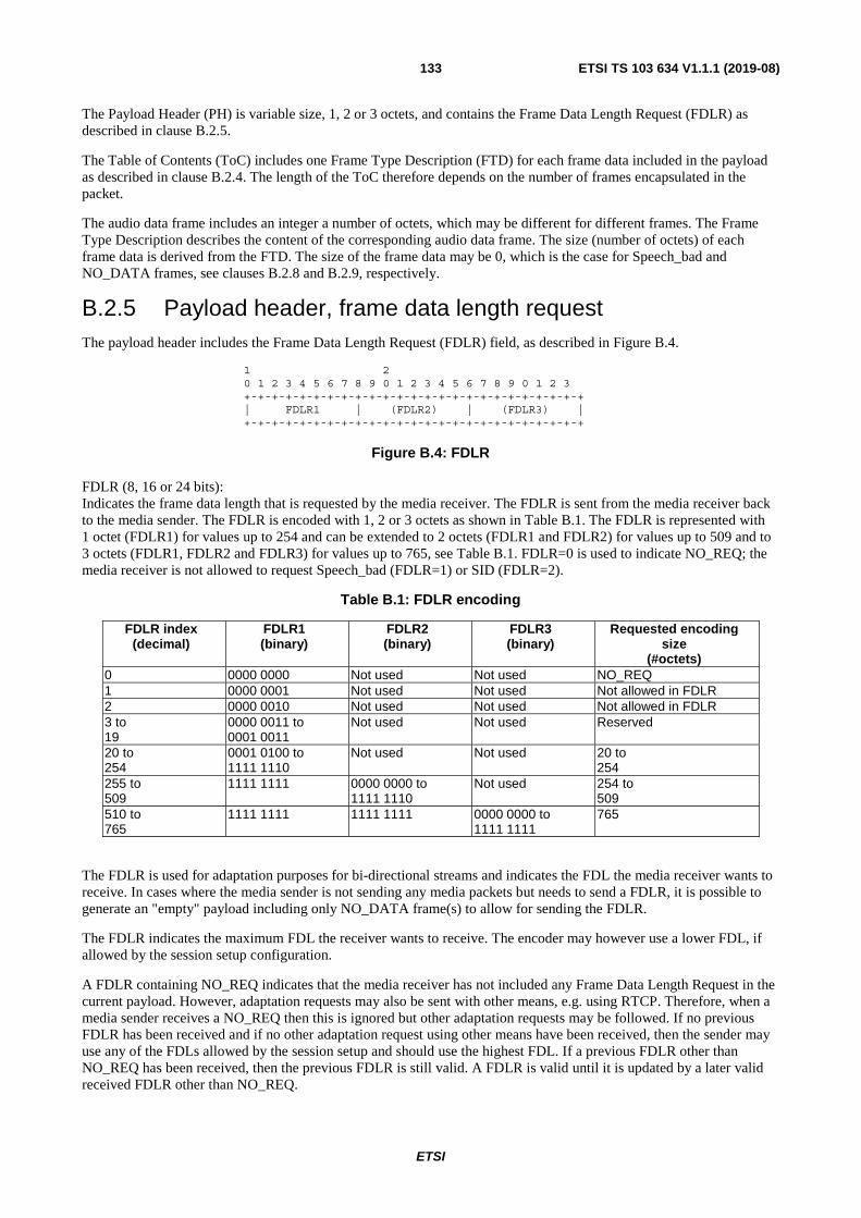
ETSI
ETSI TS 103 634 V1.1.1 (2019-08)133
The Payload Header (PH) is variable size, 1, 2 or 3 octets, and contains the Frame Data Length Request (FDLR) as described in clause B.2.5.
The Table of Contents (ToC) includes one Frame Type Description (FTD) for each frame data included in the payload as described in clause B.2.4. The length of the ToC therefore depends on the number of frames encapsulated in the packet.
The audio data frame includes an integer a number of octets, which may be different for different frames. The Frame Type Description describes the content of the corresponding audio data frame. The size (number of octets) of each frame data is derived from the FTD. The size of the frame data may be 0, which is the case for Speech_bad and NO_DATA frames, see clauses B.2.8 and B.2.9, respectively.
B.2.5 Payload header, frame data length request The payload header includes the Frame Data Length Request (FDLR) field, as described in Figure B.4.
1 2 0 1 2 3 4 5 6 7 8 9 0 1 2 3 4 5 6 7 8 9 0 1 2 3 +-+-+-+-+-+-+-+-+-+-+-+-+-+-+-+-+-+-+-+-+-+-+-+-+ | FDLR1 | (FDLR2) | (FDLR3) | +-+-+-+-+-+-+-+-+-+-+-+-+-+-+-+-+-+-+-+-+-+-+-+-+
Figure B.4: FDLR
FDLR (8, 16 or 24 bits): Indicates the frame data length that is requested by the media receiver. The FDLR is sent from the media receiver back to the media sender. The FDLR is encoded with 1, 2 or 3 octets as shown in Table B.1. The FDLR is represented with 1 octet (FDLR1) for values up to 254 and can be extended to 2 octets (FDLR1 and FDLR2) for values up to 509 and to 3 octets (FDLR1, FDLR2 and FDLR3) for values up to 765, see Table B.1. FDLR=0 is used to indicate NO_REQ; the media receiver is not allowed to request Speech_bad (FDLR=1) or SID (FDLR=2).
Table B.1: FDLR encoding
FDLR index (decimal)
FDLR1 (binary)
FDLR2 (binary)
FDLR3 (binary)
Requested encoding size
(#octets) 0 0000 0000 Not used Not used NO_REQ 1 0000 0001 Not used Not used Not allowed in FDLR 2 0000 0010 Not used Not used Not allowed in FDLR 3 to 19
0000 0011 to 0001 0011
Not used Not used Reserved
20 to 254
0001 0100 to 1111 1110
Not used Not used 20 to 254
255 to 509
1111 1111 0000 0000 to 1111 1110
Not used 254 to 509
510 to 765
1111 1111 1111 1111 0000 0000 to 1111 1111
765
The FDLR is used for adaptation purposes for bi-directional streams and indicates the FDL the media receiver wants to receive. In cases where the media sender is not sending any media packets but needs to send a FDLR, it is possible to generate an "empty" payload including only NO_DATA frame(s) to allow for sending the FDLR.
The FDLR indicates the maximum FDL the receiver wants to receive. The encoder may however use a lower FDL, if allowed by the session setup configuration.
A FDLR containing NO_REQ indicates that the media receiver has not included any Frame Data Length Request in the current payload. However, adaptation requests may also be sent with other means, e.g. using RTCP. Therefore, when a media sender receives a NO_REQ then this is ignored but other adaptation requests may be followed. If no previous FDLR has been received and if no other adaptation request using other means have been received, then the sender may use any of the FDLs allowed by the session setup and should use the highest FDL. If a previous FDLR other than NO_REQ has been received, then the previous FDLR is still valid. A FDLR is valid until it is updated by a later valid received FDLR other than NO_REQ.
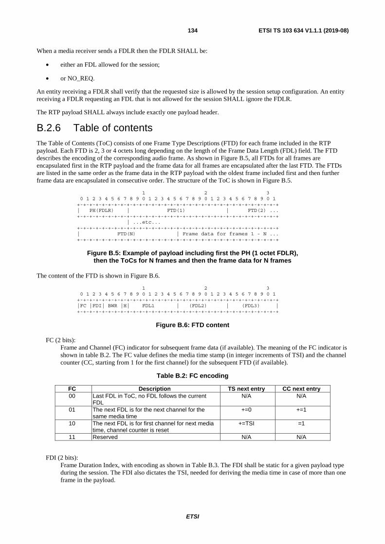
ETSI
ETSI TS 103 634 V1.1.1 (2019-08)134
When a media receiver sends a FDLR then the FDLR SHALL be:
• either an FDL allowed for the session;
• or NO_REQ.
An entity receiving a FDLR shall verify that the requested size is allowed by the session setup configuration. An entity receiving a FDLR requesting an FDL that is not allowed for the session SHALL ignore the FDLR.
The RTP payload SHALL always include exactly one payload header.
B.2.6 Table of contents The Table of Contents (ToC) consists of one Frame Type Descriptions (FTD) for each frame included in the RTP payload. Each FTD is 2, 3 or 4 octets long depending on the length of the Frame Data Length (FDL) field. The FTD describes the encoding of the corresponding audio frame. As shown in Figure B.5, all FTDs for all frames are encapsulated first in the RTP payload and the frame data for all frames are encapsulated after the last FTD. The FTDs are listed in the same order as the frame data in the RTP payload with the oldest frame included first and then further frame data are encapsulated in consecutive order. The structure of the ToC is shown in Figure B.5.
1 2 3 0 1 2 3 4 5 6 7 8 9 0 1 2 3 4 5 6 7 8 9 0 1 2 3 4 5 6 7 8 9 0 1 +-+-+-+-+-+-+-+-+-+-+-+-+-+-+-+-+-+-+-+-+-+-+-+-+-+-+-+-+-+-+-+-+ | PH(FDLR) | FTD(1) | FTD(2) ... +-+-+-+-+-+-+-+-+-+-+-+-+-+-+-+-+-+-+-+-+-+-+-+-+-+-+-+-+-+-+-+-+ | ...etc... +-+-+-+-+-+-+-+-+-+-+-+-+-+-+-+-+-+-+-+-+-+-+-+-+-+-+-+-+-+-+-+-+ | FTD(N) | Frame data for frames 1 - N ... +-+-+-+-+-+-+-+-+-+-+-+-+-+-+-+-+-+-+-+-+-+-+-+-+-+-+-+-+-+-+-+-+
Figure B.5: Example of payload including first the PH (1 octet FDLR),
then the ToCs for N frames and then the frame data for N frames
The content of the FTD is shown in Figure B.6.
1 2 3 0 1 2 3 4 5 6 7 8 9 0 1 2 3 4 5 6 7 8 9 0 1 2 3 4 5 6 7 8 9 0 1 +-+-+-+-+-+-+-+-+-+-+-+-+-+-+-+-+-+-+-+-+-+-+-+-+-+-+-+-+-+-+-+-+ |FC |FDI| BWR |H| FDL1 | (FDL2) | (FDL3) | +-+-+-+-+-+-+-+-+-+-+-+-+-+-+-+-+-+-+-+-+-+-+-+-+-+-+-+-+-+-+-+-+
Figure B.6: FTD content
FC (2 bits): Frame and Channel (FC) indicator for subsequent frame data (if available). The meaning of the FC indicator is shown in table B.2. The FC value defines the media time stamp (in integer increments of TSI) and the channel counter (CC, starting from 1 for the first channel) for the subsequent FTD (if available).
Table B.2: FC encoding
FC Description TS next entry CC next entry 00 Last FDL in ToC, no FDL follows the current
FDL N/A N/A
01 The next FDL is for the next channel for the same media time
+=0 +=1
10 The next FDL is for first channel for next media time, channel counter is reset
+=TSI =1
11 Reserved N/A N/A
FDI (2 bits): Frame Duration Index, with encoding as shown in Table B.3. The FDI shall be static for a given payload type during the session. The FDI also dictates the TSI, needed for deriving the media time in case of more than one frame in the payload.
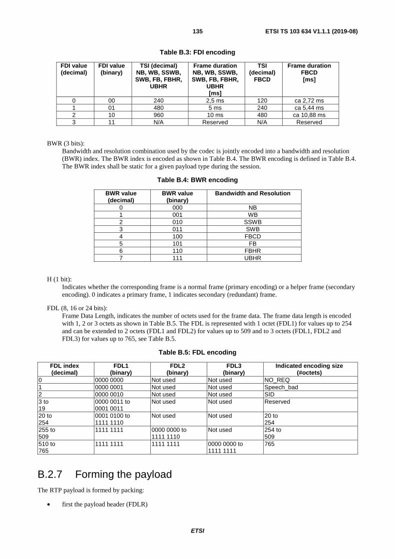
ETSI
ETSI TS 103 634 V1.1.1 (2019-08)135
Table B.3: FDI encoding
FDI value (decimal)
FDI value (binary)
TSI (decimal) NB, WB, SSWB, SWB, FB, FBHR,
UBHR
Frame duration NB, WB, SSWB, SWB, FB, FBHR,
UBHR [ms]
TSI (decimal)
FBCD
Frame duration FBCD [ms]
0 00 240 2,5 ms 120 ca 2,72 ms 1 01 480 5 ms 240 ca 5,44 ms 2 10 960 10 ms 480 ca 10,88 ms 3 11 N/A Reserved N/A Reserved
BWR (3 bits): Bandwidth and resolution combination used by the codec is jointly encoded into a bandwidth and resolution (BWR) index. The BWR index is encoded as shown in Table B.4. The BWR encoding is defined in Table B.4. The BWR index shall be static for a given payload type during the session.
Table B.4: BWR encoding
BWR value (decimal)
BWR value (binary)
Bandwidth and Resolution
0 000 NB 1 001 WB 2 010 SSWB 3 011 SWB 4 100 FBCD 5 101 FB 6 110 FBHR 7 111 UBHR
H (1 bit): Indicates whether the corresponding frame is a normal frame (primary encoding) or a helper frame (secondary encoding). 0 indicates a primary frame, 1 indicates secondary (redundant) frame.
FDL (8, 16 or 24 bits): Frame Data Length, indicates the number of octets used for the frame data. The frame data length is encoded with 1, 2 or 3 octets as shown in Table B.5. The FDL is represented with 1 octet (FDL1) for values up to 254 and can be extended to 2 octets (FDL1 and FDL2) for values up to 509 and to 3 octets (FDL1, FDL2 and FDL3) for values up to 765, see Table B.5.
Table B.5: FDL encoding
FDL index (decimal)
FDL1 (binary)
FDL2 (binary)
FDL3 (binary)
Indicated encoding size (#octets)
0 0000 0000 Not used Not used NO_REQ 1 0000 0001 Not used Not used Speech_bad 2 0000 0010 Not used Not used SID 3 to 19
0000 0011 to 0001 0011
Not used Not used Reserved
20 to 254
0001 0100 to 1111 1110
Not used Not used 20 to 254
255 to 509
1111 1111 0000 0000 to 1111 1110
Not used 254 to 509
510 to 765
1111 1111 1111 1111 0000 0000 to 1111 1111
765
B.2.7 Forming the payload The RTP payload is formed by packing:
• first the payload header (FDLR)
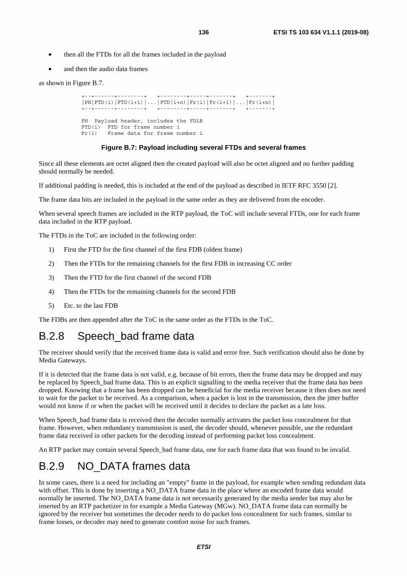
ETSI
ETSI TS 103 634 V1.1.1 (2019-08)136
• then all the FTDs for all the frames included in the payload
• and then the audio data frames
as shown in Figure B.7.
+--+------+--------+ +--------+-----+-------+ +-------+ |PH|FTD(i)|FTD(i+1)|...|FTD(i+n)|Fr(i)|Fr(i+1)|...|Fr(i+n)| +--+------+--------+ +--------+-----+-------+ +-------+ PH Payload header, includes the FDLR FTD(i) FTD for frame number i Fr(i) Frame data for frame number i
Figure B.7: Payload including several FTDs and several frames
Since all these elements are octet aligned then the created payload will also be octet aligned and no further padding should normally be needed.
If additional padding is needed, this is included at the end of the payload as described in IETF RFC 3550 [2].
The frame data bits are included in the payload in the same order as they are delivered from the encoder.
When several speech frames are included in the RTP payload, the ToC will include several FTDs, one for each frame data included in the RTP payload.
The FTDs in the ToC are included in the following order:
1) First the FTD for the first channel of the first FDB (oldest frame)
2) Then the FTDs for the remaining channels for the first FDB in increasing CC order
3) Then the FTD for the first channel of the second FDB
4) Then the FTDs for the remaining channels for the second FDB
5) Etc. to the last FDB
The FDBs are then appended after the ToC in the same order as the FTDs in the ToC.
B.2.8 Speech_bad frame data The receiver should verify that the received frame data is valid and error free. Such verification should also be done by Media Gateways.
If it is detected that the frame data is not valid, e.g. because of bit errors, then the frame data may be dropped and may be replaced by Speech_bad frame data. This is an explicit signalling to the media receiver that the frame data has been dropped. Knowing that a frame has been dropped can be beneficial for the media receiver because it then does not need to wait for the packet to be received. As a comparison, when a packet is lost in the transmission, then the jitter buffer would not know if or when the packet will be received until it decides to declare the packet as a late loss.
When Speech_bad frame data is received then the decoder normally activates the packet loss concealment for that frame. However, when redundancy transmission is used, the decoder should, whenever possible, use the redundant frame data received in other packets for the decoding instead of performing packet loss concealment.
An RTP packet may contain several Speech_bad frame data, one for each frame data that was found to be invalid.
B.2.9 NO_DATA frames data In some cases, there is a need for including an "empty" frame in the payload, for example when sending redundant data with offset. This is done by inserting a NO_DATA frame data in the place where an encoded frame data would normally be inserted. The NO_DATA frame data is not necessarily generated by the media sender but may also be inserted by an RTP packetizer in for example a Media Gateway (MGw). NO_DATA frame data can normally be ignored by the receiver but sometimes the decoder needs to do packet loss concealment for such frames, similar to frame losses, or decoder may need to generate comfort noise for such frames.
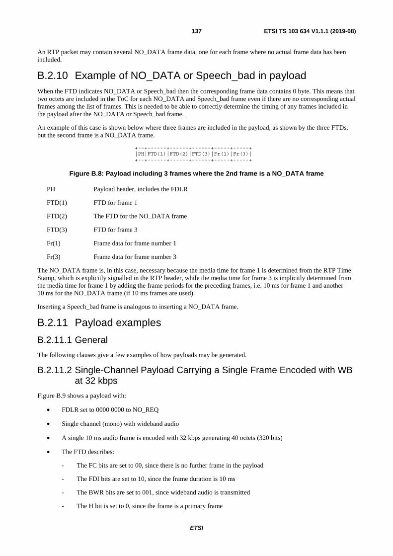
ETSI
ETSI TS 103 634 V1.1.1 (2019-08)137
An RTP packet may contain several NO_DATA frame data, one for each frame where no actual frame data has been included.
B.2.10 Example of NO_DATA or Speech_bad in payload When the FTD indicates NO_DATA or Speech_bad then the corresponding frame data contains 0 byte. This means that two octets are included in the ToC for each NO_DATA and Speech_bad frame even if there are no corresponding actual frames among the list of frames. This is needed to be able to correctly determine the timing of any frames included in the payload after the NO_DATA or Speech_bad frame.
An example of this case is shown below where three frames are included in the payload, as shown by the three FTDs, but the second frame is a NO_DATA frame.
+--+------+------+------+-----+-----+ |PH|FTD(1)|FTD(2)|FTD(3)|Fr(1)|Fr(3)| +--+------+------+------+-----+-----+
Figure B.8: Payload including 3 frames where the 2nd frame is a NO_DATA frame
PH Payload header, includes the FDLR
FTD(1) FTD for frame 1
FTD(2) The FTD for the NO_DATA frame
FTD(3) FTD for frame 3
Fr(1) Frame data for frame number 1
Fr(3) Frame data for frame number 3
The NO_DATA frame is, in this case, necessary because the media time for frame 1 is determined from the RTP Time Stamp, which is explicitly signalled in the RTP header, while the media time for frame 3 is implicitly determined from the media time for frame 1 by adding the frame periods for the preceding frames, i.e. 10 ms for frame 1 and another 10 ms for the NO_DATA frame (if 10 ms frames are used).
Inserting a Speech_bad frame is analogous to inserting a NO_DATA frame.
B.2.11 Payload examples
B.2.11.1 General
The following clauses give a few examples of how payloads may be generated.
B.2.11.2 Single-Channel Payload Carrying a Single Frame Encoded with WB at 32 kbps
Figure B.9 shows a payload with:
• FDLR set to 0000 0000 to NO_REQ
• Single channel (mono) with wideband audio
• A single 10 ms audio frame is encoded with 32 kbps generating 40 octets (320 bits)
• The FTD describes:
- The FC bits are set to 00, since there is no further frame in the payload
- The FDI bits are set to 10, since the frame duration is 10 ms
- The BWR bits are set to 001, since wideband audio is transmitted
- The H bit is set to 0, since the frame is a primary frame

ETSI
ETSI TS 103 634 V1.1.1 (2019-08)138
- The FDL field is set to 40 (0010 1000), since the size of the encoded frame is 40 octets
• The frame data is represented with d(0)-d(319)
The payload size is 43 octets.
0 1 2 3 0 1 2 3 4 5 6 7 8 9 0 1 2 3 4 5 6 7 8 9 0 1 2 3 4 5 6 7 8 9 0 1 +-+-+-+-+-+-+-+-+-+-+-+-+-+-+-+-+-+-+-+-+-+-+-+-+-+-+-+-+-+-+-+-+ |0 0 0 0 0 0 0 0|0 0:1 0:0 0 1:0:0 0 1 0 1 0 0 0|d(0) | +-+-+-+-+-+-+-+-+-+-+-+-+-+-+-+-+-+-+-+-+-+-+-+-+-+-+-+-+-+-+-+-+ | : : : | +-+-+-+-+-+-+-+-+-+-+-+-+-+-+-+-+-+-+-+-+-+-+-+-+-+-+-+-+-+-+-+-+ | : : : | +-+-+-+-+-+-+-+-+-+-+-+-+-+-+-+-+-+-+-+-+-+-+-+-+-+-+-+-+-+-+-+-+ | : : : | +-+-+-+-+-+-+-+-+-+-+-+-+-+-+-+-+-+-+-+-+-+-+-+-+-+-+-+-+-+-+-+-+ | : : : | +-+-+-+-+-+-+-+-+-+-+-+-+-+-+-+-+-+-+-+-+-+-+-+-+-+-+-+-+-+-+-+-+ | : : : | +-+-+-+-+-+-+-+-+-+-+-+-+-+-+-+-+-+-+-+-+-+-+-+-+-+-+-+-+-+-+-+-+ | : : : | +-+-+-+-+-+-+-+-+-+-+-+-+-+-+-+-+-+-+-+-+-+-+-+-+-+-+-+-+-+-+-+-+ | : : : | +-+-+-+-+-+-+-+-+-+-+-+-+-+-+-+-+-+-+-+-+-+-+-+-+-+-+-+-+-+-+-+-+ | : : : | +-+-+-+-+-+-+-+-+-+-+-+-+-+-+-+-+-+-+-+-+-+-+-+-+-+-+-+-+-+-+-+-+ | : : : | +-+-+-+-+-+-+-+-+-+-+-+-+-+-+-+-+-+-+-+-+-+-+-+-+-+-+-+-+-+-+-+-+ | : : d(319)| +-+-+-+-+-+-+-+-+-+-+-+-+-+-+-+-+-+-+-+-+-+-+-+-+
Figure B.9: Payload including one 10 ms frame encoded at 32 kbps
The RTP Time Stamp is set to represent the media time of the beginning of the 10 ms frame (first audio sample in the input frame).
B.2.11.3 Single-Channel Payload Carrying a Single Frame Encoded with SWB at 64 kbps
Figure B.10 shows a payload with:
• FDLR set to 0000 0000 to NO_REQ
• Single channel (mono) with superwideband audio
• A single 10 ms audio frame is encoded with 64 kbps generating 80 octets (640 bits)
• The FTD describes:
- The FC bits are set to 00, since there is no further frame in the payload
- The FDI bits are set to 10, since the frame duration is 10 ms
- The BWR bits are set to 011, since superwideband audio is transmitted
- The H bit is set to 0, since the frame is a primary frame
- The FDL field is set to 80 (0101 0000), since the size of the encoded frame is 80 octets
• The frame data is represented with d(0)-d(639)
The payload size is 83 octets.

ETSI
ETSI TS 103 634 V1.1.1 (2019-08)139
0 1 2 3 0 1 2 3 4 5 6 7 8 9 0 1 2 3 4 5 6 7 8 9 0 1 2 3 4 5 6 7 8 9 0 1 +-+-+-+-+-+-+-+-+-+-+-+-+-+-+-+-+-+-+-+-+-+-+-+-+-+-+-+-+-+-+-+-+ |0 0 0 0 0 0 0 0|0 0:1 0:0 0 1:0:0 0 1 0 1 0 0 0|d(0) | +-+-+-+-+-+-+-+-+-+-+-+-+-+-+-+-+-+-+-+-+-+-+-+-+-+-+-+-+-+-+-+-+ | : : : | +-+-+-+-+-+-+-+-+-+-+-+-+-+-+-+-+-+-+-+-+-+-+-+-+-+-+-+-+-+-+-+-+ | : : : | +-+-+-+-+-+-+-+-+-+-+-+-+-+-+-+-+-+-+-+-+-+-+-+-+-+-+-+-+-+-+-+-+ | : : : | +-+-+-+-+-+-+-+-+-+-+-+-+-+-+-+-+-+-+-+-+-+-+-+-+-+-+-+-+-+-+-+-+ | : : : | +-+-+-+-+-+-+-+-+-+-+-+-+-+-+-+-+-+-+-+-+-+-+-+-+-+-+-+-+-+-+-+-+ | : : : | +-+-+-+-+-+-+-+-+-+-+-+-+-+-+-+-+-+-+-+-+-+-+-+-+-+-+-+-+-+-+-+-+ | : : : | +-+-+-+-+-+-+-+-+-+-+-+-+-+-+-+-+-+-+-+-+-+-+-+-+-+-+-+-+-+-+-+-+ | : : : | +-+-+-+-+-+-+-+-+-+-+-+-+-+-+-+-+-+-+-+-+-+-+-+-+-+-+-+-+-+-+-+-+ | : : : | +-+-+-+-+-+-+-+-+-+-+-+-+-+-+-+-+-+-+-+-+-+-+-+-+-+-+-+-+-+-+-+-+ | : : : | +-+-+-+-+-+-+-+-+-+-+-+-+-+-+-+-+-+-+-+-+-+-+-+-+-+-+-+-+-+-+-+-+ | : : : | +-+-+-+-+-+-+-+-+-+-+-+-+-+-+-+-+-+-+-+-+-+-+-+-+-+-+-+-+-+-+-+-+ | : : : | +-+-+-+-+-+-+-+-+-+-+-+-+-+-+-+-+-+-+-+-+-+-+-+-+-+-+-+-+-+-+-+-+ | : : : | +-+-+-+-+-+-+-+-+-+-+-+-+-+-+-+-+-+-+-+-+-+-+-+-+-+-+-+-+-+-+-+-+ | : : : | +-+-+-+-+-+-+-+-+-+-+-+-+-+-+-+-+-+-+-+-+-+-+-+-+-+-+-+-+-+-+-+-+ | : : : | +-+-+-+-+-+-+-+-+-+-+-+-+-+-+-+-+-+-+-+-+-+-+-+-+-+-+-+-+-+-+-+-+ | : : : | +-+-+-+-+-+-+-+-+-+-+-+-+-+-+-+-+-+-+-+-+-+-+-+-+-+-+-+-+-+-+-+-+ | : : : | +-+-+-+-+-+-+-+-+-+-+-+-+-+-+-+-+-+-+-+-+-+-+-+-+-+-+-+-+-+-+-+-+ | : : : | +-+-+-+-+-+-+-+-+-+-+-+-+-+-+-+-+-+-+-+-+-+-+-+-+-+-+-+-+-+-+-+-+ | : : : | +-+-+-+-+-+-+-+-+-+-+-+-+-+-+-+-+-+-+-+-+-+-+-+-+-+-+-+-+-+-+-+-+ | : : : | +-+-+-+-+-+-+-+-+-+-+-+-+-+-+-+-+-+-+-+-+-+-+-+-+-+-+-+-+-+-+-+-+ | : : d(639)| +-+-+-+-+-+-+-+-+-+-+-+-+-+-+-+-+-+-+-+-+-+-+-+-+
Figure B.10: Payload including one 10 ms frame encoded at 64 kbps
The RTP Time Stamp is set to represent the media time of the beginning of the 10 ms frame (first audio sample in the input frame).
B.2.11.4 Single-Channel Payload Carrying Two Active Frames Encoded with WB at Different Bitrates
The diagram below shows a payload with:
• FDLR set to 0010 1000 to request 40 octets (320 kbps)
• 1 channel (mono) with wideband audio
• Two 10 ms frames are encoded, the first encoded with 16 kbps generating 20 octets (160 bits), and the second frame encoded with 24 kbps generating 30 octets (240 bits)
• The FTD for the first frame describes:
- The FC bits are set to 10, since another frame follow after the first frame and since there is one channel
- The FDI bits are set to 10, since the frame duration is 10 ms
- The BWR bits are set to 001, since wideband audio is transmitted
- The H bit is set to 0, since the frame is a primary frame
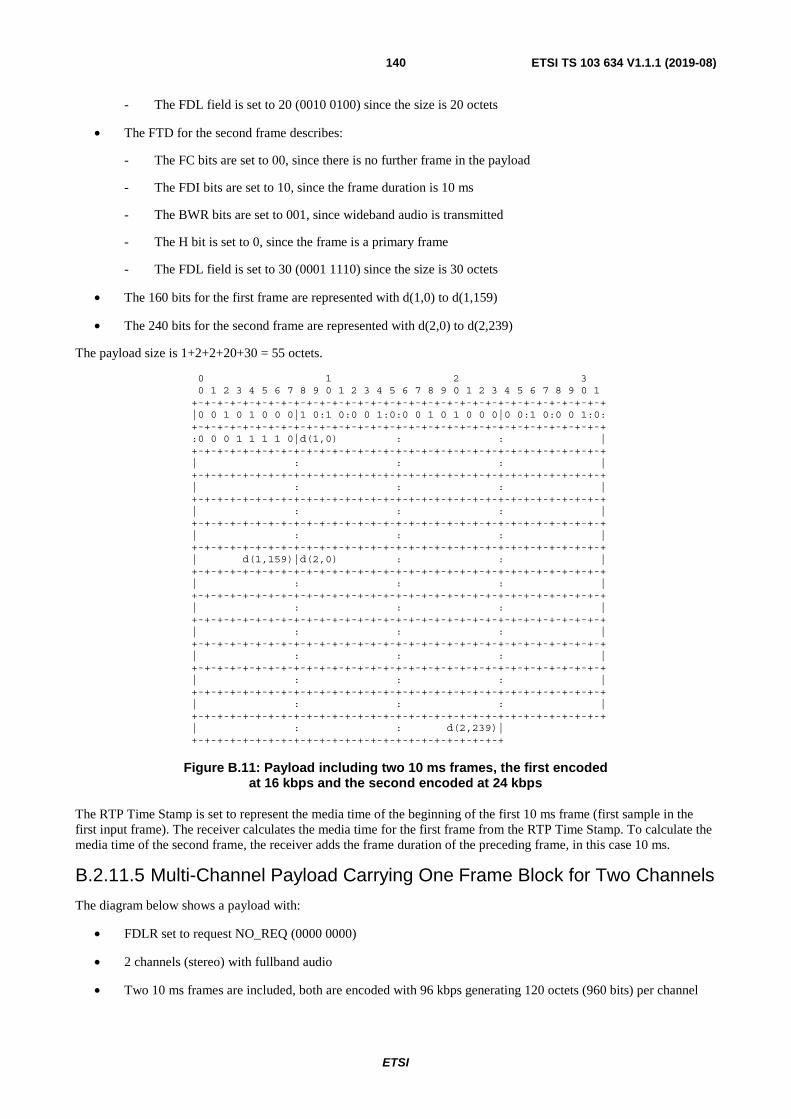
ETSI
ETSI TS 103 634 V1.1.1 (2019-08)140
- The FDL field is set to 20 (0010 0100) since the size is 20 octets
• The FTD for the second frame describes:
- The FC bits are set to 00, since there is no further frame in the payload
- The FDI bits are set to 10, since the frame duration is 10 ms
- The BWR bits are set to 001, since wideband audio is transmitted
- The H bit is set to 0, since the frame is a primary frame
- The FDL field is set to 30 (0001 1110) since the size is 30 octets
• The 160 bits for the first frame are represented with d(1,0) to d(1,159)
• The 240 bits for the second frame are represented with d(2,0) to d(2,239)
The payload size is 1+2+2+20+30 = 55 octets.
0 1 2 3 0 1 2 3 4 5 6 7 8 9 0 1 2 3 4 5 6 7 8 9 0 1 2 3 4 5 6 7 8 9 0 1 +-+-+-+-+-+-+-+-+-+-+-+-+-+-+-+-+-+-+-+-+-+-+-+-+-+-+-+-+-+-+-+-+ |0 0 1 0 1 0 0 0|1 0:1 0:0 0 1:0:0 0 1 0 1 0 0 0|0 0:1 0:0 0 1:0: +-+-+-+-+-+-+-+-+-+-+-+-+-+-+-+-+-+-+-+-+-+-+-+-+-+-+-+-+-+-+-+-+ :0 0 0 1 1 1 1 0|d(1,0) : : | +-+-+-+-+-+-+-+-+-+-+-+-+-+-+-+-+-+-+-+-+-+-+-+-+-+-+-+-+-+-+-+-+ | : : : | +-+-+-+-+-+-+-+-+-+-+-+-+-+-+-+-+-+-+-+-+-+-+-+-+-+-+-+-+-+-+-+-+ | : : : | +-+-+-+-+-+-+-+-+-+-+-+-+-+-+-+-+-+-+-+-+-+-+-+-+-+-+-+-+-+-+-+-+ | : : : | +-+-+-+-+-+-+-+-+-+-+-+-+-+-+-+-+-+-+-+-+-+-+-+-+-+-+-+-+-+-+-+-+ | : : : | +-+-+-+-+-+-+-+-+-+-+-+-+-+-+-+-+-+-+-+-+-+-+-+-+-+-+-+-+-+-+-+-+ | d(1,159)|d(2,0) : : | +-+-+-+-+-+-+-+-+-+-+-+-+-+-+-+-+-+-+-+-+-+-+-+-+-+-+-+-+-+-+-+-+ | : : : | +-+-+-+-+-+-+-+-+-+-+-+-+-+-+-+-+-+-+-+-+-+-+-+-+-+-+-+-+-+-+-+-+ | : : : | +-+-+-+-+-+-+-+-+-+-+-+-+-+-+-+-+-+-+-+-+-+-+-+-+-+-+-+-+-+-+-+-+ | : : : | +-+-+-+-+-+-+-+-+-+-+-+-+-+-+-+-+-+-+-+-+-+-+-+-+-+-+-+-+-+-+-+-+ | : : : | +-+-+-+-+-+-+-+-+-+-+-+-+-+-+-+-+-+-+-+-+-+-+-+-+-+-+-+-+-+-+-+-+ | : : : | +-+-+-+-+-+-+-+-+-+-+-+-+-+-+-+-+-+-+-+-+-+-+-+-+-+-+-+-+-+-+-+-+ | : : : | +-+-+-+-+-+-+-+-+-+-+-+-+-+-+-+-+-+-+-+-+-+-+-+-+-+-+-+-+-+-+-+-+ | : : d(2,239)| +-+-+-+-+-+-+-+-+-+-+-+-+-+-+-+-+-+-+-+-+-+-+-+-+
Figure B.11: Payload including two 10 ms frames, the first encoded
at 16 kbps and the second encoded at 24 kbps
The RTP Time Stamp is set to represent the media time of the beginning of the first 10 ms frame (first sample in the first input frame). The receiver calculates the media time for the first frame from the RTP Time Stamp. To calculate the media time of the second frame, the receiver adds the frame duration of the preceding frame, in this case 10 ms.
B.2.11.5 Multi-Channel Payload Carrying One Frame Block for Two Channels
The diagram below shows a payload with:
• FDLR set to request NO_REQ (0000 0000)
• 2 channels (stereo) with fullband audio
• Two 10 ms frames are included, both are encoded with 96 kbps generating 120 octets (960 bits) per channel
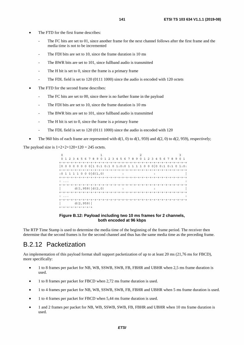
ETSI
ETSI TS 103 634 V1.1.1 (2019-08)141
• The FTD for the first frame describes:
- The FC bits are set to 01, since another frame for the next channel follows after the first frame and the media time is not to be incremented
- The FDI bits are set to 10, since the frame duration is 10 ms
- The BWR bits are set to 101, since fullband audio is transmitted
- The H bit is set to 0, since the frame is a primary frame
- The FDL field is set to 120 (0111 1000) since the audio is encoded with 120 octets
• The FTD for the second frame describes:
- The FC bits are set to 00, since there is no further frame in the payload
- The FDI bits are set to 10, since the frame duration is 10 ms
- The BWR bits are set to 101, since fullband audio is transmitted
- The H bit is set to 0, since the frame is a primary frame
- The FDL field is set to 120 (0111 1000) since the audio is encoded with 120
• The 960 bits of each frame are represented with d(1, 0) to d(1, 959) and d(2, 0) to d(2, 959), respectively;
The payload size is 1+2+2+120+120 = 245 octets.
0 1 2 3 0 1 2 3 4 5 6 7 8 9 0 1 2 3 4 5 6 7 8 9 0 1 2 3 4 5 6 7 8 9 0 1 +-+-+-+-+-+-+-+-+-+-+-+-+-+-+-+-+-+-+-+-+-+-+-+-+-+-+-+-+-+-+-+-+ |0 0 0 0 0 0 0 0|1 0:1 0:1 0 1:0:0 1 1 1 1 0 0 0|0 0:1 0:1 0 1:0: +-+-+-+-+-+-+-+-+-+-+-+-+-+-+-+-+-+-+-+-+-+-+-+-+-+-+-+-+-+-+-+-+ :0 1 1 1 1 0 0 0|d(1,0) : : | +-+-+-+-+-+-+-+-+-+-+-+-+-+-+-+-+-+-+-+-+-+-+-+-+-+-+-+-+-+-+-+-+ : ... : +-+-+-+-+-+-+-+-+-+-+-+-+-+-+-+-+-+-+-+-+-+-+-+-+-+-+-+-+-+-+-+-+ | d(1,959)|d(2,0) : : | +-+-+-+-+-+-+-+-+-+-+-+-+-+-+-+-+-+-+-+-+-+-+-+-+-+-+-+-+-+-+-+-+ : ... : +-+-+-+-+-+-+-+-+-+-+-+-+-+-+-+-+-+-+-+-+-+-+-+-+-+-+-+-+-+-+-+-+ | d(2,959)| +-+-+-+-+-+-+-+-+
Figure B.12: Payload including two 10 ms frames for 2 channels,
both encoded at 96 kbps
The RTP Time Stamp is used to determine the media time of the beginning of the frame period. The receiver then determine that the second frames is for the second channel and thus has the same media time as the preceding frame.
B.2.12 Packetization An implementation of this payload format shall support packetization of up to at least 20 ms (21,76 ms for FBCD), more specifically:
• 1 to 8 frames per packet for NB, WB, SSWB, SWB, FB, FBHR and UBHR when 2,5 ms frame duration is used.
• 1 to 8 frames per packet for FBCD when 2,72 ms frame duration is used.
• 1 to 4 frames per packet for NB, WB, SSWB, SWB, FB, FBHR and UBHR when 5 ms frame duration is used.
• 1 to 4 frames per packet for FBCD when 5,44 ms frame duration is used.
• 1 and 2 frames per packet for NB, WB, SSWB, SWB, FB, FBHR and UBHR when 10 ms frame duration is used.
ETSI
ETSI TS 103 634 V1.1.1 (2019-08)142
• 1 and 2 frames per packet for FBCD when 10,88 ms frame duration is used.
This is because it is common to transmit about 50 packets per second for VoIP services. Furthermore, this also reduces the IP/UDP/RTP overhead that otherwise would become quite extensive when sending frequent small packets.
This does not mean that every packet will always include the maximum number of allowed frames, but also payloads with fewer frames shall be supported, enabling applications with lower latency at the expense of higher packet rate.
The packetization in a session is typically decided by the ptime value negotiated at session setup. However, this does not mean that the negotiated packetization is used for the entire session. The packetization may be both smaller and larger than the ptime value but is limited to the maxptime value (if negotiated).
B.3 Payload format parameters
B.3.1 General This clause defines parameters of the LC3plus payload format.
This media type registration covers real-time transfer via RTP and non-real-time transfers via stored files. All media type parameters defined in this clause shall be supported. The receiver shall ignore any unspecified parameter.
The registrations are done following IETF RFC 4855 [5] and the media registration rules IETF RFC 3264 [1].
B.3.2 LC3plus media type registration Media type name: Audio
Media subtype name: LC3plus
Required parameters: Either bwr or both bwr-recv and bwr-send shall be included.
Either fdi or both fdi-recv and fdi-send shall be included.
Optional parameters: All remaining parameters specified below are optional
The parameters defined below apply to RTP transfer only.
ptime: See IETF RFC 4566 [4].
maxptime: See IETF RFC 4566 [4].
fdl: Specifies the Frame Data Length (FDL) in integer number of octets, the set of FDLs or the FDL range allowed in the session for the send and the received directions. The parameter can either have a single value (fdl1), a comma-separated list (fdl1, fdl2, …, fdlN) of values or a hyphen-separated pair of two values (fdl1-fdl2). When a single value is included, then this FDL is the only allowed FDL. When a comma-separated list is included, then all listed FDLs are allowed and FDLs that are not listed are not allowed. When a hyphen-separated pair of values is used, then fdl1 defines the minimum FDL allowed and fdl2 defines the maximum FDL allowed. Any FDLs in-between these values are also allowed. The fdl1 value shall be smaller than fdl2 value. If the fdl parameter is not present, and if neither fdl-recv nor fdl-send are present, then all integer sizes are allowed.
fdl-recv: Specifies the FDL, the set of FDLs or the FDL range allowed in the session for the received direction, otherwise the same as the fdl parameter. If both fdl and fdl-recv are included, then fdl-recv takes precedence over fdl.
ETSI
ETSI TS 103 634 V1.1.1 (2019-08)143
fdl-send: Specifies the FDL, the set of FDLs or the FDL range allowed in the session for the send direction, otherwise the same as the fdl parameter. If both fdl and fdl-send are included, then fdl-send takes precedence over fdl.
bwr: Specifies the audio bandwidth and resolution (BWR) combination for the send and the receive direction. During session setup, the parameter can either have a single value (bwr1) or comma-separated list (bwr1, bwr2, …, bwrN). When a comma-separated list is used, the bwr shall be listed with the lowest BWR value first and the remaining BWRs in increasing order, for example "bwr=nb,wb,sswb,swb". It is not permitted to indicate fbcd in combination with any of the other BWRs. This is because FBCD uses a different RTP clock rate than the audio bandwidths. If it is desired to allow for FBCD and other audio bandwidths in a session, then a different RTP definition (different RTP payload type numbers) shall be used.
bwr-recv: Specifies the audio bandwidth and resolution combinations for the receive direction, otherwise the same as the bwr parameter. If both bwr and bwr-recv are included, the bwr-recv takes precedence over bwr.
bwr-send: Specifies the audio bandwidth and resolution combinations allowed in the session for the send direction, otherwise the same as the bwr parameter. If both bwr and bwr-send are included, the bwr-send takes precedence over bwr.
channels: The number of audio channels per frame data block. See IETF RFC 3551 [3]. This parameter is included on the a=rtpmap line, for example "a=rtpmap: LC3plus/96000/1" where "/1" indicates the number of channels. If the channels parameter is not present, its default value is 1. If both ch-send and ch-recv are included (see below) with different numbers of channels for sending and receiving directions, channels is set to the larger of the two values.
ch-recv: Specifies the number of audio channels to be used in the session for the receive direction. The ch-recv parameter can be a single value, which is a strictly positive integer, i.e. 1 to any larger integer. If ch-recv is not present, and if channels (see above) is not present, then ch-recv=1, mono, is used.
ch-send: Specifies the number of audio channels to be used in the session for the send direction. The ch-send parameter can be a single value, which is a strictly positive integer, i.e. 1 to any larger integer. If ch-send is not present, and if channels (see above) is not present, then ch-send=1, mono, is used.
fdi: Specifies the Frame Duration Index (FDI) in decimal form from Table B.3 allowed in the session for the send and the receive direction. During session setup, the parameter can either have a single value (fdi1) or a comma-separated list (fdi1, fdi2, …, fdiN). When a comma-separated list is used, the FDIs shall be listed in increasing order.
fdi-recv: Specifies the FDI in decimal form from Table B.3 allowed in the session for the receive direction, otherwise the same as the fdi parameter. If both fdi and fdi-recv are included, then fdi-recv takes precedence over fdi.
fdi-send: Specifies the FDI in decimal form from Table B.3 allowed in the session for the send direction, otherwise the same as the fdi parameter. If both fdi and fdi-send are included, then fdi-send takes precedence over fdi.
max-red: See IETF RFC 4867 [6].
rfdl: Specifies the redundant FDL in integer number of octets, where the redundancy is created by the LC3plus codec. The parameter can either be a single value ("rfdl=pr1"), a comma-separated list ("rfdl=rfdl1,rfdl2,…, rfdlN") or a range ("pred=rfdl1-rfdl2").
ETSI
ETSI TS 103 634 V1.1.1 (2019-08)144
Including the rfdl parameter in the SDP means that codec redundancy is supported but is not required to be used. Omitting the rfdl parameter in the SDP means that codec redundancy is not to be used. This parameter does not control the packetization redundancy created by the LC3plus payload format.
rfdl-recv: Specifies the redundant FDL, the set of redundant FDLs or the redundant FDL range allowed in the session for receiving direction, otherwise the same as the rfdl parameter. If both rfdl and rfdl-recv are included, then rfdl-recv takes precedence over rfdl.
rfdl-send: Specifies the redundant FDL, the set of redundant FDLs or the redundant FDL range allowed in the session for sending direction, otherwise the same as the rfdl parameter. If both rfdl and rfdl-send are included, then rfdl-send takes precedence over rfdl.
B.3.3 Mapping media type parameters into SDP The information carried in the media type specification has a specific mapping to fields in the Session Description Protocol (SDP) IETF RFC 4566 [4], which is commonly used to describe RTP sessions. When SDP is used to specify sessions employing the LC3plus codec, the mapping is as follows:
• The media type ("audio") goes in SDP "m=" as the media name.
• The media subtype (payload format name) goes in SDP "a=rtpmap" as the encoding name. The RTP clock rate in "a=rtpmap" shall be set according to clause B.2.2.4 and the encoding parameters (number of channels) shall either be explicitly set to N or omitted, implying a default value of 1. The values of N that are allowed are specified in Section 4.1 in IETF RFC 3551 [3].
• The parameters "ptime" and "maxptime" go in the SDP "a=ptime" and "a=maxptime" attributes, respectively.
• Any remaining parameters go in the SDP "a=fmtp" attribute by copying them directly from the media type parameter string as a semicolon-separated list of parameter=value pairs.
B.3.4 Offer-answer model considerations The following considerations apply when using SDP Offer-Answer procedures to negotiate the use of LC3plus payload in RTP:
fdl: If the SDP offer included a FDL range, it is permissible to include a FDL range, a comma-separated list of FDLs or a single FDL in the SDP answer. If the SDP offer included a comma-separated list of FDLs, it is permissible to include a comma-separated list or a single FDL in the SDP answer but not a FDL range. If the SDP offer includes a single FDL, the answerer shall either accept this or reject the payload type. The answerer is in this case not allowed to change the value. The value(s) in the fdl in the SDP answer shall be identical to or a subset of the value(s) in the fdl in the SDP offer.
fdl-recv: The value(s) for fdl-send or fdl shall be identical to or a subset of fdl-recv for the payload type in the SDP offer.
fdl-send: The value(s) for fdl-recv or fdl shall be identical to or a subset of fdl-send for the payload type in the SDP offer.
bwr: The offerer may indicate several BWR values in the SDP offer but the answerer SHALL select one BWR from the offered BWR values and include this in the SDP answer. If the offerer wants to allow for switching between audio bandwidths and/or resolutions within a session, for example to allow for switching between NB, WB and SWB, then the SDP offer needs to include one RTP definition (one RTP payload type number) for each respective audio bandwidth and resolution combination.
ETSI
ETSI TS 103 634 V1.1.1 (2019-08)145
bwr-recv When bwr-recv is offered for a payload type and the payload is accepted, the answerer shall select one of the indicated BWR values and include this in the bwr-send parameter in the SDP answer.
bwr-send: When bwr-send is offered for a payload type and the payload is accepted, the answerer shall select one of the indicated BWR values and include this in the bwr-recv parameter in the SDP answer.
channels: See <encoding parameters> of a=rtpmap attribute specified in IETF RFC 4566 [4] and clause B.3.2.
ch-recv: When ch-recv is offered for a payload type and the payload type is accepted, the answerer shall include ch-send in the SDP answer, and the ch-send shall be identical to the ch-recv parameter for the payload type in the SDP offer.
ch-send: When ch-send is offered for a payload type and the payload type is accepted, the answerer shall include ch-recv in the SDP answer, and the ch-recv shall be identical to the ch-send parameter for the payload type in the SDP offer.
fdi: The offerer may indicate several FDI values in the SDP offer but the answerer shall select one FDI from the offered FDI values and include this in the SDP answer. If the offerer wants to allow for switching between frame durations, for example to allow both 5 ms and 10 ms frame durations, then the SDP offer needs to include one RTP definition (one RTP payload type number) for each respective frame duration.
fdi-recv: When fdi-recv is offered for a payload type and the payload is accepted, the answerer shall include fdi-send in the SDP answer, and shall select one of the indicated FDI values.
fdi-send: When fdi-send is offered for a payload type and the payload is accepted, the answerer shall include fdi-recv in the SDP answer, and shall select one of the indicated FDI values.
rfdl: If the SDP offer included a redundant FDL range, it is permissible to include a redundant FDL range, a comma-separated list of redundant FDLs, a single redundant FDL or reject the redundant FDL in the SDP answer. If the SDP offer included a comma-separated list of redundant FDLs, it is permissible to include a comma-separated list, a single redundant FDL or reject the redundant FDL in the SDP answer but not a redundant FDL range. If the SDP offer includes a single redundant FDL, the answerer shall either accept this or reject the redundant FDL.
rfdl-recv: When rfdl-recv is offered for a payload type and the payload type is accepted, the answerer may include rfdl-send in the SDP answer, and the rfdl-send shall be identical to or a subset of rfdl-recv for the payload type in the SDP offer.
rfdl-send: When rfdl-send is offered for a payload type and the payload type is accepted, the answerer may include rfdl-recv in the SDP answer, and the rfdl-recv shall be identical to or a subset of rfdl-send for the payload type in the SDP offer.
B.3.5 SDP examples
B.3.5.1 General
A number of SDP offer/answer examples are included below to describe different aspects of the session negotiation for several session variants.
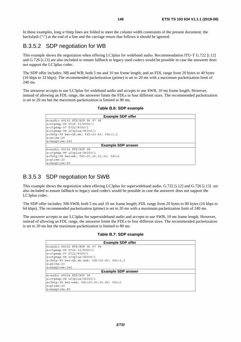
ETSI
ETSI TS 103 634 V1.1.1 (2019-08)146
In these examples, long a=fmtp lines are folded to meet the column width constraints of the present document; the backslash ("\") at the end of a line and the carriage return that follows it should be ignored.
B.3.5.2 SDP negotiation for WB
This example shows the negotiation when offering LC3plus for wideband audio. Recommendation ITU-T G.722 [i.12] and G.726 [i.13] are also included to ensure fallback to legacy used codecs would be possible in case the answerer does not support the LC3plus codec.
The SDP offer includes: NB and WB; both 5 ms and 10 ms frame length; and an FDL range from 20 bytes to 40 bytes (16 kbps to 32 kbps). The recommended packetization (ptime) is set to 20 ms with a maximum packetization limit of 240 ms.
The answerer accepts to use LC3plus for wideband audio and accepts to use SWB, 10 ms frame length. However, instead of allowing an FDL range, the answerer limits the FDLs to four different sizes. The recommended packetization is set to 20 ms but the maximum packetization is limited to 80 ms.
Table B.6: SDP example
Example SDP offer m=audio 49152 RTP/AVP 96 97 98 a=rtpmap:96 G726-32/8000/1 a=rtpmap:97 G722/8000/1 a=rtpmap:98 LC3plus/96000/1 a=fmtp:98 bwr=nb,wb; fdl=20-40; fdi=1,2 a=ptime:20 a=maxptime:240
Example SDP answer m=audio 49154 RTP/AVP 98 a=rtpmap:98 LC3plus/96000/1 a=fmtp:98 bwr=wb; fdl=20,26,32,36; fdi=2 a=ptime:20 a=maxptime:80
B.3.5.3 SDP negotiation for SWB
This example shows the negotiation when offering LC3plus for superwideband audio. G.722 [i.12] and G.726 [i.13] are also included to ensure fallback to legacy used codecs would be possible in case the answerer does not support the LC3plus codec.
The SDP offer includes: NB-SWB; both 5 ms and 10 ms frame length; FDL range from 20 bytes to 80 bytes (16 kbps to 64 kbps). The recommended packetization (ptime) is set to 20 ms with a maximum packetization limit of 240 ms.
The answerer accepts to use LC3plus for superwideband audio and accepts to use SWB, 10 ms frame length. However, instead of allowing an FDL range, the answerer limits the FDLs to four different sizes. The recommended packetization is set to 20 ms but the maximum packetization is limited to 80 ms.
Table B.7: SDP example
Example SDP offer m=audio 49152 RTP/AVP 96 97 98 a=rtpmap:96 G726-32/8000/1 a=rtpmap:97 G722/8000/1 a=rtpmap:98 LC3plus/96000/1 a=fmtp:98 bwr=nb,wb,swb; fdl=20-80; fdi=1,2 a=ptime:20 a=maxptime:240
Example SDP answer m=audio 49154 RTP/AVP 98 a=rtpmap:98 LC3plus/96000/1 a=fmtp:98 bwr=swb; fdl=20,40,60,80; fdi=2 a=ptime:20 a=maxptime:80

ETSI
ETSI TS 103 634 V1.1.1 (2019-08)147
B.4 IANA considerations One media type (LC3plus/audio) has been updated, see clause B.3.

ETSI
ETSI TS 103 634 V1.1.1 (2019-08)148
Annex C (informative): Change History
Date Version Information about changes 2019-06-19 0.1.0 First complete version for review and approval
2019-06-26 0.1.1 Added terms and abbreviations for RTP payload format in Annex B Minor editorial updates

ETSI
ETSI TS 103 634 V1.1.1 (2019-08)149
History
Document history
V1.1.1 August 2019 Publication
Ì


