Page 1
HAL Id: pastel-00001877https://pastel.archives-ouvertes.fr/pastel-00001877
Submitted on 13 Nov 2006
HAL is a multi-disciplinary open accessarchive for the deposit and dissemination of sci-entific research documents, whether they are pub-lished or not. The documents may come fromteaching and research institutions in France orabroad, or from public or private research centers.
L’archive ouverte pluridisciplinaire HAL, estdestinée au dépôt et à la diffusion de documentsscientifiques de niveau recherche, publiés ou non,émanant des établissements d’enseignement et derecherche français ou étrangers, des laboratoirespublics ou privés.
Etude Multi-couches dans le système HSDPAMohamad Assaad
To cite this version:Mohamad Assaad. Etude Multi-couches dans le système HSDPA. domain_other. Télécom ParisTech,2006. English. pastel-00001877
Page 2
These
presentee pour obtenir le grade de Docteur de
l’Ecole Nationale Superieure Des Telecommunications
Mohamad ASSAAD
ETUDE MULTI-COUCHES DANS LE SYSTEME HSDPA
soutenue le 06 Mars 2006 devant le jury compose de:
Prof. Jean-Claude Belfiore President ENST Paris, France
Prof. Khaled Ben Letaief Rapporteur University of Science and Technology, Hong Kong
Prof. Hamid Aghvami Rapporteur King’s College, Londres
Prof. Hikmet Sari Examinateur Supelec, France
Dr. Mongi Marzoug Examinateur Orange, France
Prof. Djamal Zeghlache Directeur de these INT Evry, France
Departement Rereaux et Services Multimedia Mobiles
Institut National des Telecommunications (INT)
Evry - France
Page 3
Dissertation
presented in partial fulfillment of the requirements for the degree of
DOCTOR OF PHILOSOPHY
of
Ecole Nationale Superieure Des Telecommunications
Mohamad ASSAAD
CROSS LAYER STUDY IN HSDPA SYSTEM
The committee in charge is formed by:
Prof. Jean-Claude Belfiore Committee chair ENST Paris, France
Prof. Khaled Ben Letaief Reviewer University of Science and Technology, Hong Kong
Prof. Hamid Aghvami Reviewer King’s College, London
Prof. Hikmet Sari Examiner Supelec, France
Dr. Mongi Marzoug Examiner Orange, France
Prof. Djamal Zeghlache Thesis Director INT Evry, France
Mobile Networks and Multimedia Services Department
Institut National des Telecommunications (INT)
Evry - France
March 2006
Page 4
iii
”To My Family”
Page 5
iv
Acknowledgements
The work on this thesis has been an inspiring, exciting and interesting experience. First and foremost, I would
like to express my deepest sense of gratitude to my supervisor Prof Djamal Zeghlache for his encouragement,
support and excellent advice over the past years. His valuable technical helps and constructive suggestions were
a source of inspiration and motivation all along my way. Our hours-lasting discussions on technical and non-
technical issues have enriched my experience and paved my way to the finish line. Thanks Djamal for your nice
humanitarian attitude and your friendship that I want to last for many more years.
I am greatly grateful to Professors Khaled Ben Letaief and Hamid Aghvami to accept to review this thesis
despite their busy routine. They have enriched my knowledge with their valuable comments and exceptional
insights into the telecommunications. Many thanks go also to Dr Mongi Marzoug and professors Hikmet sari and
Jean-Claude Belfiore who honored me by their participation to my thesis committee.
I am really indebted to all the members of the Mobile Networks and Multimedia Services department at INT
for the convivial and family environment within the department. I can not omit mentioning our angel Isabelle
who ran to our help especially when we had difficulties with the French Bureaucracy. Over the past three years,
I built a friendship with my office colleague Wajdi Louati. Special thanks to you Wajdi for your support, help
and everything we shared especially during the famous ”pauses cafe”. It is now your turn to defend your PhD.
Good luck!
This paragraph would certainly be incomplete if I did not mention my family who gave me unconditional
support and love. I express my profound gratitude to them for being helpful and supportive all along my way.
Page 6
v
Abstract
The increased use of Internet and data services motivates the evolution of cellular networks from second
to third generation and beyond. The UMTS (Universal Mobile for Telecommunications System) has prepared
for this evolution in successive releases within the third generation partnership project (3GPP). In this context,
HSDPA (High Speed Downlink Packet Access) has been developed in releases 5 and 6 by introducing a number of
additional enhancements (Hybrid ARQ, Adaptive Modulation and Coding or AMC and fast scheduling over time
shared channels) into the standard to enable flexible and adaptive packet transmissions and to offer Internet and
multimedia based services. The efficiency of these introduced features depends essentially upon the interactions
of these techniques with the higher and lower layers (physical, transport, application,...). Cross layer interactions
can have a drastic impact on overall throughput and capacity. This thesis focuses on the analysis and modeling
of these cross layer interactions between the new MAC-hs entity (Medium Access Control high speed) of HSDPA
and the upper and lower layers. The objective is to find the best configuration of this new entity to minimize the
negative interaction between layers and optimize the performance of HSDPA. Consequently, this thesis provides
comprehensive modeling studies covering the following topics or aspects:
• Analysis and modeling of the effect of wireless channel (shadowing, fast fading,...) on the HSDPA system
performance and efficiency for various scheduling algorithms. Several uncorrelated and correlated fading
models are considered in this study.
• Analysis and modeling of the effect of Circuit Switched (CS) services transmitted on the UMTS Release 99
(R99) Dedicated Physical Channels (DPCHs). This analysis can serve to provide guidelines for the UMTS
planning process when resources are dynamically shared between circuit and packet services.
• Characterization and modeling of the interaction between TCP protocol and the MAC-hs layer result-
ing from the introduction of Hybrid-ARQ and scheduling features into the network. A new scheduler is
suggested to reduce this interaction and improve the system performance and efficiency.
• Characterization of the interaction of the MAC-hs with the streaming services. A new opportunistic
scheduler is proposed to achieve better trade-off between fairness and cell capacity, in other words to
guarantee stringent QoS constraints (delay, jitter,...) of streaming services without losing much cell capacity.
System simulations using NS2 (Network Simulator) are used to assess the accuracy of the analytical conducted
studies.
Page 7
vi
Resume
L’augmentation de l’utilisation de l’Internet et des services de donnees motive l’evolution des reseaux cellulaires
de la deuxieme a la troisieme et ”apres troisieme” generations (3G and beyond en anglais). L’UMTS (Universal
Mobile for Telecommunications System) a ete prepare pour cette evolution a travers les versions successives
(releases) de la norme developpees au sein du 3GPP (third generation partnership project). Dans ce contexte,
HSDPA (High Speed Downlink Packet Access) a ete developpe dans les releases 5 et 6 pour poursuivre l’volution
du mode ”paquet” de l’UMTS. Ce systeme utilise de nouvelles technologies telles que le Hybrid-ARQ (Automatic
Repeat Request), la modulation adaptative en presence d’une adaptation de lien et l’ordonnancement rapide (fast
Scheduling) pour permettre de vehiculer des debits plus eleves sur l’interface radio et d’augmenter la capacite. En
deuxieme phase, la technologie Multi-antennes MIMO (Multiple Input Multiple Output) est prevue d’etre utilisee
afin d’accroıtre la capacite radio et permettre d’integrer des services a des debits plus eleves. L’efficacite et les
performances des techniques utilisees dans HSDPA dependent essentiellement des interactions entre les differentes
couches physique, transport, application, etc. Ces interactions peuvent affecter le debit de chaque utilisateur et
avoir, par la suite, des consequences sur la capacite et l’efficacite globales du systeme. Cette these se focalise sur
l’analyse et la modelisation des interactions entre la couche MAC-hs (Medium Access Control - high speed) de
HSDPA et les autres couches (physique, transport). L’objectif est de trouver la configuration optimale de cette
entite MAC-hs afin de reduire les interactions ”negatives” entre-couches et optimiser les performances de HSDPA.
Par consequent, cette these fournit des etudes et des modelisations analytiques couvrant les aspects suivants:
• Analyse et modelisation de l’impact du canal radio (shadowing, fast fading,...) sur l’efficacite et les perfor-
mances du systeme HSDPA dans le cas ou plusieurs algorithmes d’ordonnancement sont utilises. Plusieurs
modeles de ”fading” correles et d-correles sont consideres dans cette etude.
• Analyse et modelisation de l’effect des services ”Circuit” CS (Circuit Switched) sur les performances de
HSDPA. Ces services sont vehicules sur les canaux dedies DPCHs (Dedicated Physical Channels) de l’UMTS
(release 99) et partagent simultanement les memes ressources cellulaires que HSDPA. Cette etude pourra
servir dans la plannification de l’UMTS ou les ressources sont partagees dynamiquement et simultanement
entre les services ”circuit” et ”packet”.
• Characterisation et modelisation de l’interaction entre le protocole TCP et l’entite MAC-hs. Cette inter-
action est due essentiellement a l’utilisation des techniques Hybrid-ARQ et ordonnancement (scheduling)
dans le systeme. Une nouvelle strategie d’ordonnancement est proposee dans cette partie de la these afin
de reduire cette interaction et ameliorer les performances du systeme.
• Characterisation de l’interaction entre l’entite MAC-hs et les services streaming ayant de fortes contraintes
de QoS (Quality of Service). Une nouvelle strategie d’ordonnancement dite opprotunistique est proposee
afin d’atteindre un meilleur compromis entre l’equite et la capacite de la cellule, autrement afin de garantir
les contraintes severes de QoS (delai, gigue,...) des services streaming sans trop perdre de capacite cellulaire.
Page 8
vii
Une simulation ”systeme” utilisant le logiciel NS2 (Network Simulator) a ete utilisee pour valider les etudes
analytiques menees tout au long de cette these.
Page 9
viii
Publications of the author
Book
1. Mohamad Assaad and Djamal Zeghlache, TCP over UMTS-HSDPA Systems, To be published byCRC Press, Francis and Taylor Auerbach Publications, New York, ISBN: 0849368383, 224 pages,(expected 19/07/2006).
Journals
1. Mohamad Assaad and Djamal Zeghlache, ”Effect of Circuit Switched Services on HSDPA CellCapacity ”, IEEE Transactions on Wireless Communications, Vol. 5, Issue 5, May 2006, pp.1044-1054.
2. Mohamad Assaad and Djamal Zeghlache, ”Cross Layer Design in HSDPA System ”, IEEE Journalon Selected Areas in Communications (JSAC), Vol. 24, No. 3, March 2006, pp. 614-625.
3. M. Assaad and D. Zeghlache, ”How to minimize the TCP Effect in a UMTS-HSDPA System”,Wiley Wireless Communications and Mobile Computing (WCMC), June 2005, vol. 5 issue 4, pp.473-485.
4. M. Assaad, B. Jouaber and D. Zeghlache, ”TCP Performance over UMTS-HSDPA System”,Kluwer on Telecommunication Systems 27:2-4, 371-391, 2004.
5. Mohamad Assaad and Djamal Zeghlache, ”A Simple SIR Distribution For Correlated Dense Mul-tipath Channel And Its Application to HSDPA Cell Capacity Analysis,” IEEE transactions onwireless communications Letters, second round review.
6. Mohamad Assaad and Djamal Zeghlache, ”Opportunistic Scheduler for HSDPA System ”, IEEETransactions on Wireless Communications, submitted.
7. Mohamad Assaad and Djamal Zeghlache, ”Resource Allocation for Circuit Switched and PacketSwitched Services in a Combined UMTS R99/HSDPA System”, IEEE Transactions on VehicularTechnology, submitted.
8. Mohamad Assaad and Djamal Zeghlache, ”HSDPA Performance Under Nakagami Fading Chan-nel”, IEEE Transactions on Wireless Communications, second round review.
Conferences
1. M. Assaad, B. Jouaber and D. Zeghlache, ”Effect of TCP on UMTS/HSDPA System Performanceand Capacity”, IEEE Global Telecommunications Conference, GLOBECOM ’04, Dallas. Volume:6 , 29 Nov.-3 Dec., 2004, Pages:4104 - 4108.
2. M. Assaad and D. Zeghlache, ”Scheduler Study in HSDPA System”, IEEE PIMRC 2005, Sep.2005.
3. M. Assaad and D. Zeghlache, ”On the Capacity of HSDPA System”, Global TelecommunicationsConference, 2003. GLOBECOM ’03. IEEE ,Volume: 1, 1-5 Dec. 2003, Pages: 60 - 64.
4. M. Assaad and D. Zeghlache, ”Comparison between MIMO techniques in a UMTS-HSDPA Sys-tem”, IEEE International Symposium on Spread Sprectrum Techniques and Applications ISSSTA,30 Aug.-2 Sept. 2004, Sydney, Pages 874-878.
Page 10
ix
5. M. Assaad and D. Zeghlache, ”Fast Scheduling in HSDPA System: A Trade-off Between Fairnessand Efficiency”, IEEE WPMC 2005, Sep. 2005.
6. M. Assaad and D. Zeghlache, ”MIMO/HSDPA with Fast Fading and Mobility: Capacity andCoverage Study”, 15th IEEE International Symposium on Personal, Indoor and Mobile RadioCommunications, PIMRC 2004, Volume: 3 , 5-8 Sept. 2004, Barcelona, Pages:2181 - 2186.
7. M. Assaad, B. Jouaber and D. Zeghlache, ”TCP Performance over UMTS-HSDPA System”,ICN’04 Guadeloupe, French Caribbean, March 2004, Vol.2, (Gosier, February-Mars 2004), p.874-878.
8. M. Assaad and D. Zeghlache, ”Opportunistic Scheduler for Streaming Services in HSDPA system,”to appear in IEEE PIMRC 2006, Helsinki, Finland, 11-14 September, 2006.
Page 11
x
Description generale des travaux menes dans cette these
Depuis le debut des annees 1990, les services de communications cellulaires connaissent un developpement
sans precedent, rendu possible par l’existence de technologies numeriques dites de 2e generation, le GSM
etant l’une des plus populaires. Les systemes mobiles de 2e generation sont conus pour offrir des services
de transmission de la voix et des donnees de faible debit. Cependant, Le mode de fonctionnement ”
donnees ” est en train de prendre du terrain sur le mode ” voix ”. Pour permettre la creation de nouveaux
services et d’offrir aux usagers une veritable itinerance a l’echelle mondiale, il etait devenu necessaire
d’effectuer un saut technologique et de franchir le pas vers les reseaux cellulaires de 3e generation. Le
nom UMTS (Universal Mobile for Telecommunication System) a ete choisi par l’organisme de stan-
dardisation de telecommunication europeenne ETSI (European Telecommunication Standard Institute)
pour les systemes de troisieme generation. La technique CDMA (Code Division Multiple Access) est
adoptee comme mode d’acces et de partage de la ressource. L’UMTS utilise sur l’interface radio deux
modes : UTRA FDD (UMTS Terrestrial Radio Access Frequency Division Duplex) base sur la tech-
nique WCDMA pur (Wideband Code Division Multiple Access) et UTRA TDD (UMTS Terrestrial
Radio Access Time Division Duplex) base sur la combinaison TDMA-CDMA (Time Division Multiple
Access Code Division Multiple Access).
Les systemes futurs de communications mobiles large bande sont appeles a fournir la capacite d’acces
suffisante a un nombre croissant d’utilisateurs combine a une densification du trafic de type ” Internet
mobile ”. Vu que la capacite du systeme UMTS, comme tous les systemes utilisant le CDMA, est
limitee par la sensibilite du CDMA aux interferences, les etudes se sont concentrees depuis la fin de
l’annee 2000 sur l’evolution de l’interface radio de l’UMTS dans le but de repondre au defi ci dessus.
HSDPA (High Speed Downlink Packet Access) est l’une des solutions proposees. Ce systeme utilise de
nouvelles technologies telles que le Hybrid-ARQ, la modulation adaptative en presence d’une adaptation
de lien et l’ordonnancement rapide (fast Scheduling) pour permettre de vehiculer des debits plus eleves
sur l’interface radio et d’augmenter la capacite. En deuxieme phase, la technologie Multi-antennes
MIMO (Multiple Input Multiple Output) est prevue d’etre utilisee afin d’accroıtre la capacite radio
et permettre d’integrer des services a des debits plus eleves. En effet, l’utilisation de modulations
d’ordre eleve permet d’atteindre des debits plus eleves sur la voie descendante. Par contre, Ceci peut
degrader les performances du systeme surtout en absence de controle de puissance. Pour y faire face,
on procede a une adaptation rapide de lien combinee a un mecanisme de HARQ. Ce mecanisme permet
de retransmettre les paquets errones jusqu’a reception de l’information. Une combinaison dite ”douce”
Page 12
xi
des differentes retransmissions est utilisee en HSDPA afin de diminuer le nombre de retransmissions. Le
but est d’envisager une augmentation du debit du canal et par la suite d’accroıtre la capacite jusqu’a
14.4 Mbps par secteur.
Les contributions essentielles des travaux de recherche dans cette these s’inscrivent dans le contexte
de l’etude des interactions entre les couches physique, MAC, Transport et application. Le but est de
trouver l’apport de ces interactions sur la capacite totale et les performances des systemes mobiles.
Ces etudes ont ete menees analytiquement en utilisant des outils mathematiques et statistiques. Une
simulation dite ” systeme ” est ensuite utilisee pour valider les algorithmes et modeles analytiques
proposes. Les travaux de recherche menes tout au long de cette these peuvent divises en quatre majeures
parties:
1. Effet du canal radio sur les performances des algorithmes d’ordonnancement (chapitre 3)
2. Interaction des services voix de l’UMTS Release 99 avec les services Data de HSDPA (chapitre 4)
3. Interaction de la couche MAC-hs avec le protocole TCP de la couche transport (chapitre 5)
4. Interaction de la couche MAC-hs avec les services streaming (chapitre 6)
Cette these est divisee en sept chapitres. Les contributions essentielles sont decrites dans les chapitres
3 a 6. Chapitre 1 presente une introduction generale aux problematiques abordees en decrivant les
motivations et les contributions apportees. Chapitre 2 presente une description generale du systeme
HSDPA. Les conclusions et les eventuelles perspectives sont presentees dans le chapitre 7.
1. Effet du canal radio sur les performances de HSDPA (chapitre 3)
En HSDPA, le couplage de ” Adaptation de lien ” / ” ordonnancement (Scheduling) ” controle les allo-
cations d’acces en mode paquet. Il permet de partager le canal de transport des donnees, dit HS-DSCH,
entre les utilisateurs et de gerer la charge du systeme. En effet, le Scheduler decide a quel utilisateur
le canal HS-DSCH sera dedie dans le prochain slot. L’adaptation de lien utilisant la technique AMC
(Adaptive Modulation and Coding) est utilisee ensuite afin d’adapter les parametres de transmissions
aux variations rapides (fast fading) du canal radio. L’allocation de ressources (AMC+scheduling) doit
tenir compte des conditions radios de chaque utilisateur ainsi que du delai tolere par chaque service.
Plusieurs strategies d’ordonnancement peuvent etre utilisees dans ce cas. La strategie Max C/I con-
siste a allouer le canal a l’utilisateur qui a les meilleures conditions radios ce qui permet d’utiliser des
Page 13
xii
modulations et des codages d’ordre plus eleve et d’accroıtre ainsi la capacite du systeme. Ce genre
d’ordonnancement risque de bloquer des utilisateurs situes en bordure de la cellule et dont le lien radio
n’est pas toujours le plus favorable. Une autre strategie consiste a allouer le canal aux utilisateurs de telle
faon a avoir une repartition equitable de ressources entre les utilisateurs autrement dit a avoir le meme
debit final par utilisateur (dit Fair Throughput). Cette strategie respecte les contraintes temporelles
des services mais ne permet pas d’optimiser la capacite. Dans la litterature, plusieurs algorithmes
d’ordonnancement ont ete proposes afin de trouver un compromis entre la maximisation de la capacite
et le respect des contraintes temporelles. Citons par exemple, le Proportional Fair (PF) et le Score
Based (SB). La maximisation de la capacite et la performance de l’allocation de ressources en general
dependent de plusieurs facteurs : les conditions radios et plus precisement l’environnement radio (e.g.
macro, micro, shadowing, fast fading,), le recepteur utilise (e.g. Rake) ainsi le type des services utilises.
Cette partie de la these presente des etudes statistiques sur l’effet du canal radio (plusieurs modeles
de fast fading et des canaux multi-trajet avec et sans correlation) sur les performances de HSDPA en
presence de plusieurs algorithmes d’ordonnancement et d’un recepteur de type ” Rake ”. Ces etudes
se sont concentrees sur les trafics FTP uniquement (services non temps reel). Une simulation systeme
utilisant le logiciel NS2 est utilisee pour valider les etudes analytiques elaborees.
2. Interaction des services ”circuit” de l’UMTS Release 99 avec les
services Data de HSDPA (chapitre 4)
Les services ” donnees ” offerts par HSDPA seront utilises en parallele avec les services ” circuit ” de
l’UMTS Release 99. L’effet de ces derniers sur la capacite de HSDPA n’a pas eu assez d’attention des
les etudes deja existantes dans la litterature. Les services voix ” speech ” ont toujours la priorite par
rapport aux services donnees a cause de leurs contraintes temporelles severes. Ces services ” circuit ”
utilisent le meme arbre de code que les utilisateurs HSDPA. En plus, ils consomment une partie de la
puissance du node B et exercent une interference supplementaire sur le canal HS-DSCH de HSDPA.
Par consequent, il faut trouver la capacite que peut offrir HSDPA en presence des services circuits (e.g.
voix, services donnees a contrainte faible LCD ou Low Constraint Data). Dans cette partie, on propose
un modele permettant de calculer la capacite du HSDPA en presence des services ” circuit ”. Les memes
algorithmes etudies dans la phase precedente ont ete etudies a nouveau en presence des services ” circuit
” afin de trouver l’effet de ces derniers sur les performances de HSDPA dans plusieurs environnements
Page 14
xiii
radio. Les etudes analytiques menees dans cette partie ont ete validees par une simulation systeme
utilisant le logiciel NS2.
3. Interaction de la couche MAC-hs (Medium Access Control - high
speed) de HSDPA avec le protocole TCP de la couche transport (chapitre
5)
TCP (Transport Control Protocol) est un protocole qui assure une transmission fiable des donnees et
un controle de flux au niveau de la couche transport. Ceci est assure par l’utilisation d’un mecanisme
de transmission a fenetre glissante couple avec un mecanisme de retransmission des segments TCP
errones et un controle de la taille de la fenetre de transmission en fonction des congestions dans les
reseaux. TCP est utilise comme protocole de transport dans la majorite des services vehicules sur
Internet (presque 90%) et il est prevu d’occuper une large partie des services ” donnees ” vehicules
dans les reseaux mobiles de troisieme generation. Dans les reseaux sans fil, les erreurs sur l’interface
radio sont interpretees par TCP comme etant des congestions ce qui entraıne une retransmission des
segments TCP contenant les erreurs et une baisse de la taille de la fenetre de transmission. Ceci entraıne
une baisse de la capacite totale du systeme et une perte d’efficacite du a une baisse de la fenetre sans
qu’il y ait de congestion (autrement sans un reel besoin de cette baisse). L’utilisation de Hybrid-ARQ
resout en partie ce probleme. En effet, ARQ retransmet les paquets errones au niveau de la couche
MAC-hs empechant ainsi le transfert des erreurs a la couche transport. Par consequent, les erreurs
causees par l’interface radio seront transparentes par rapport a la couche transport. Cependant, le
mecanisme Hybrid-ARQ genere un delai de reception du aux retransmissions frequentes des paquets. Si
ce delai est important (ce qui est le cas malheureusement a cause des erreurs frequentes sur l’interface
radio), un phenomene de ” timeout ” surgit (i.e. un timer declenche au moment de la transmission du
segment TCP expire sans recevoir un acquittement du recepteur indiquant la reception du segment sans
erreur). TCP mal interprete ce delai comme etant du a une congestion et declenche un mecanisme de
retransmission suivi d’une baisse de la fenetre de transmission jusqu’a sa valeur initiale entraınant ainsi
une perte d’efficacite et une baisse de la capacite totale du systeme. Dans cette partie de la these, on
a developpe une analyse mathematique de ce probleme en proposant un modele analytique capable de
determiner quantitativement l’effet des algorithmes d’ordonnancement (etudies precedemment) sur les
performances services TCP vehicules sur HSDPA. Un nouvel algorithme d’ordonnancement est propose
Page 15
xiv
afin de minimiser l’aspect negatif de cette interaction entre les couches TCP et MAC-hs et ameliorer
ainsi les performances de HSDPA dans le cas des services non temps reel utilisant TCP comme couche
de transport. Ces etudes analytiques sont ensuite validees par simulation systeme sou NS2.
4. Interaction de la couche MAC-hs avec les services streaming (chapitre
6)
Cette partie decrit les etudes menees pour analyser l’interaction entre la couche MAC-hs (AMC+scheduling+HARQ)
et les services streaming ayant des contraintes temporelles plus severes que les services non temps reel.
Le but est de voir si l’on peut faire passer des services streaming sur HSDPA avec un minimum de cout,
autrement dit sans trop perdre de capacite. En effet, une caracteristique fondamentale des services
streaming est de maintenir la gigue sous un certain seuil. Ce seuil depend essentiellement du debit du
trafic et de la capacite de stockage du recepteur. L’utilisation d’un buffer a la reception permet de lisser
la gigue du trafic et reduire ainsi la sensibilite de l’application aux delais.
Dans cette these, on s’est concentre uniquement sur les services streaming a debit constant egal a
128kbps (Constant Bit Rate ou CBR). Les resultats ont montre que les schedulers traditionnels tels
que le Proportional Fair ne sont adaptes aux contraintes des services streaming. La variation du debit
durant la connexion ne permet pas d’offrir des services streaming a un grand nombre d’utilisateurs
dans la cellule. Cette partie s’est aboutie a une proposition d’un nouvel algorithme d’ordonnancement
capable de vehiculer du streaming sur HSDPA sans trop perdre de capacite cellulaire. Autrement dit,
cet algorithme permet d’atteindre un meilleur compromis entre ” la capacite cellulaire ” et ” l’equite”
que les schedulers traditionnels.
Page 16
Contents
1 General Introduction and Thesis Contribution 3
1.1 General Introduction . . . . . . . . . . . . . . . . . . . . . . . . . . . . . . . . . . . . . . 3
1.2 Thesis Objectives . . . . . . . . . . . . . . . . . . . . . . . . . . . . . . . . . . . . . . . . 4
1.3 Thesis Contributions . . . . . . . . . . . . . . . . . . . . . . . . . . . . . . . . . . . . . . 6
1.3.1 Effect of radio channel models on HSDPA performance (chapter 3) . . . . . . . . 7
1.3.2 Interaction of HSDPA services with Circuit Switched services transmitted on
UMTS R99 dedicated channels (chapter 4) . . . . . . . . . . . . . . . . . . . . . 8
1.3.3 Interaction of MAC-hs and schedulers with the TCP protocol (chapter 5) . . . . 9
1.3.4 Interaction of MAC-hs and schedulers with Streaming services (chapter 6) . . . . 9
2 High Speed Downlink Packet Access (HSDPA) 11
2.1 HSDPA Concept . . . . . . . . . . . . . . . . . . . . . . . . . . . . . . . . . . . . . . . . 12
2.2 Channels Structure . . . . . . . . . . . . . . . . . . . . . . . . . . . . . . . . . . . . . . . 14
2.2.1 HS-DSCH Channel . . . . . . . . . . . . . . . . . . . . . . . . . . . . . . . . . . . 14
2.2.2 HS-SCCH Channel . . . . . . . . . . . . . . . . . . . . . . . . . . . . . . . . . . . 15
2.2.3 HS-DPCCH Channel . . . . . . . . . . . . . . . . . . . . . . . . . . . . . . . . . . 15
2.3 MAC-hs . . . . . . . . . . . . . . . . . . . . . . . . . . . . . . . . . . . . . . . . . . . . . 16
2.4 Fast Link Adaptation . . . . . . . . . . . . . . . . . . . . . . . . . . . . . . . . . . . . . 16
2.5 Adaptive Modulation and Coding . . . . . . . . . . . . . . . . . . . . . . . . . . . . . . . 18
2.6 Hybrid-ARQ . . . . . . . . . . . . . . . . . . . . . . . . . . . . . . . . . . . . . . . . . . 19
2.6.1 Hybrid-ARQ types . . . . . . . . . . . . . . . . . . . . . . . . . . . . . . . . . . . 20
2.6.2 HARQ Protocol . . . . . . . . . . . . . . . . . . . . . . . . . . . . . . . . . . . . 20
2.7 Packet Scheduling . . . . . . . . . . . . . . . . . . . . . . . . . . . . . . . . . . . . . . . 21
2.7.1 Scheduling Constraints and Parameters . . . . . . . . . . . . . . . . . . . . . . . 22
xv
Page 17
xvi CONTENTS
2.7.2 Selected Scheduling algorithms . . . . . . . . . . . . . . . . . . . . . . . . . . . . 23
3 Scheduling of Non-real Time Data: Analytical Studies 31
3.1 Introduction . . . . . . . . . . . . . . . . . . . . . . . . . . . . . . . . . . . . . . . . . . . 31
3.2 Signal to Interference Ratio (SIR) expression . . . . . . . . . . . . . . . . . . . . . . . . 32
3.2.1 Transmitted signal . . . . . . . . . . . . . . . . . . . . . . . . . . . . . . . . . . . 32
3.2.2 Channel model . . . . . . . . . . . . . . . . . . . . . . . . . . . . . . . . . . . . . 33
3.2.3 Receiver output . . . . . . . . . . . . . . . . . . . . . . . . . . . . . . . . . . . . . 36
3.2.4 SIR expression . . . . . . . . . . . . . . . . . . . . . . . . . . . . . . . . . . . . . 37
3.3 HSDPA analytical models . . . . . . . . . . . . . . . . . . . . . . . . . . . . . . . . . . . 38
3.3.1 Hybrid-ARQ . . . . . . . . . . . . . . . . . . . . . . . . . . . . . . . . . . . . . . 38
3.3.2 Fast cell selection . . . . . . . . . . . . . . . . . . . . . . . . . . . . . . . . . . . . 39
3.3.3 Adaptive Modulation and Coding (AMC) . . . . . . . . . . . . . . . . . . . . . . 40
3.3.4 Scheduling . . . . . . . . . . . . . . . . . . . . . . . . . . . . . . . . . . . . . . . 54
3.4 Network Simulation . . . . . . . . . . . . . . . . . . . . . . . . . . . . . . . . . . . . . . 65
3.5 Results . . . . . . . . . . . . . . . . . . . . . . . . . . . . . . . . . . . . . . . . . . . . . . 66
3.6 Conclusion . . . . . . . . . . . . . . . . . . . . . . . . . . . . . . . . . . . . . . . . . . . 81
4 Interaction of HSDPA with Circuit Switched (CS) Services 87
4.1 Part I: Circuit Switched services analysis . . . . . . . . . . . . . . . . . . . . . . . . . . . 88
4.1.1 Distribution of the sum of CS services required powers . . . . . . . . . . . . . . . 89
4.1.2 Evaluation of E(Pcs) and σ2(Pcs) . . . . . . . . . . . . . . . . . . . . . . . . . . . 90
4.1.3 Relation between the maximum number of HS-DSCH codes N and Ncs . . . . . . 95
4.2 Part II: HSDPA Analysis . . . . . . . . . . . . . . . . . . . . . . . . . . . . . . . . . . . 95
4.2.1 Adaptive Modulation and Coding (AMC) . . . . . . . . . . . . . . . . . . . . . . 96
4.2.2 Scheduling . . . . . . . . . . . . . . . . . . . . . . . . . . . . . . . . . . . . . . . 99
4.3 Simulation and Results . . . . . . . . . . . . . . . . . . . . . . . . . . . . . . . . . . . . . 103
4.3.1 Monte Carlo Simulation . . . . . . . . . . . . . . . . . . . . . . . . . . . . . . . . 103
4.3.2 NS Simulation . . . . . . . . . . . . . . . . . . . . . . . . . . . . . . . . . . . . . 104
4.3.3 Results . . . . . . . . . . . . . . . . . . . . . . . . . . . . . . . . . . . . . . . . . 104
4.3.4 Remark . . . . . . . . . . . . . . . . . . . . . . . . . . . . . . . . . . . . . . . . . 106
4.4 Conclusion . . . . . . . . . . . . . . . . . . . . . . . . . . . . . . . . . . . . . . . . . . . 110
Page 18
CONTENTS xvii
5 Interaction of HSDPA with Transport Control Protocol (TCP) 113
5.1 Related Work . . . . . . . . . . . . . . . . . . . . . . . . . . . . . . . . . . . . . . . . . . 114
5.2 Modeling of TCP over UMTS/HSDPA . . . . . . . . . . . . . . . . . . . . . . . . . . . . 116
5.2.1 Timeout . . . . . . . . . . . . . . . . . . . . . . . . . . . . . . . . . . . . . . . . . 117
5.2.2 Slow Start . . . . . . . . . . . . . . . . . . . . . . . . . . . . . . . . . . . . . . . . 118
5.2.3 Recovery time of the first loss . . . . . . . . . . . . . . . . . . . . . . . . . . . . . 119
5.2.4 Steady State phase . . . . . . . . . . . . . . . . . . . . . . . . . . . . . . . . . . . 120
5.3 Simulation and Results . . . . . . . . . . . . . . . . . . . . . . . . . . . . . . . . . . . . . 121
5.3.1 NS-2 Simulation . . . . . . . . . . . . . . . . . . . . . . . . . . . . . . . . . . . . 121
5.3.2 Results . . . . . . . . . . . . . . . . . . . . . . . . . . . . . . . . . . . . . . . . . 122
5.3.3 Discussions and Proposals to improve the TCP performance . . . . . . . . . . . . 124
5.4 Conclusion . . . . . . . . . . . . . . . . . . . . . . . . . . . . . . . . . . . . . . . . . . . 127
6 Scheduling of Streaming Services in HSDPA 135
6.1 Streaming Services . . . . . . . . . . . . . . . . . . . . . . . . . . . . . . . . . . . . . . . 136
6.1.1 Streaming Session protocols . . . . . . . . . . . . . . . . . . . . . . . . . . . . . . 137
6.1.2 Streaming Video Encoding . . . . . . . . . . . . . . . . . . . . . . . . . . . . . . 138
6.2 Related Work and proposed scheduler . . . . . . . . . . . . . . . . . . . . . . . . . . . . 138
6.2.1 Proposed scheduler . . . . . . . . . . . . . . . . . . . . . . . . . . . . . . . . . . . 140
6.3 Network Simulation . . . . . . . . . . . . . . . . . . . . . . . . . . . . . . . . . . . . . . 140
6.4 Results . . . . . . . . . . . . . . . . . . . . . . . . . . . . . . . . . . . . . . . . . . . . . . 141
6.5 Conclusion . . . . . . . . . . . . . . . . . . . . . . . . . . . . . . . . . . . . . . . . . . . 142
7 Conclusions and Future Work 151
7.1 Summary of Research . . . . . . . . . . . . . . . . . . . . . . . . . . . . . . . . . . . . . 151
7.1.1 Effect of radio channel models on HSDPA performance (chapter 3) . . . . . . . . 152
7.1.2 Interaction of HSDPA services with Circuit Switched services transmitted on
UMTS R99 (chapter 4) . . . . . . . . . . . . . . . . . . . . . . . . . . . . . . . . 152
7.1.3 Interaction of MAC-hs and schedulers with TCP protocol (chapter 5) . . . . . . 153
7.1.4 Interaction of MAC-hs and schedulers with Streaming services (chapter 6) . . . . 154
7.2 Future Research . . . . . . . . . . . . . . . . . . . . . . . . . . . . . . . . . . . . . . . . 154
Page 20
List of Figures
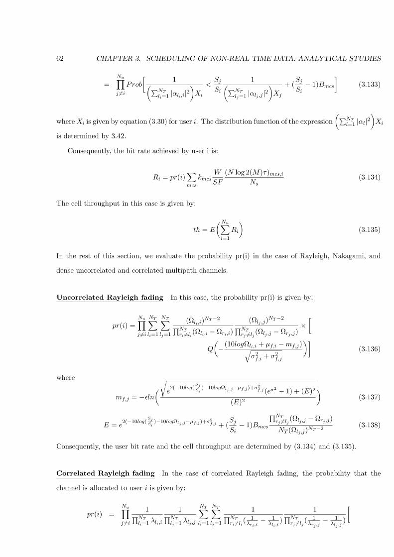
3.1 CDF of the bit rate of a user situated at 800m from the node B in the case of Max C/I
scheduler and Rayleigh fast fading . . . . . . . . . . . . . . . . . . . . . . . . . . . . . . 67
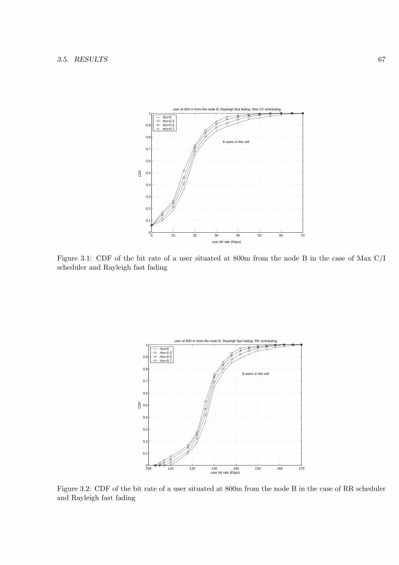
3.2 CDF of the bit rate of a user situated at 800m from the node B in the case of RR scheduler
and Rayleigh fast fading . . . . . . . . . . . . . . . . . . . . . . . . . . . . . . . . . . . . 67
3.3 CDF of the bit rate of a user situated at 800m from the node B in the case of PF scheduler
and Rayleigh fast fading . . . . . . . . . . . . . . . . . . . . . . . . . . . . . . . . . . . . 68
3.4 CDF of the bit rate of a user situated at 800m from the node B in the case of SB scheduler
and Rayleigh fast fading . . . . . . . . . . . . . . . . . . . . . . . . . . . . . . . . . . . . 68
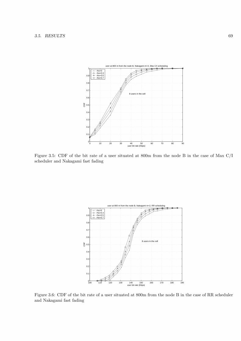
3.5 CDF of the bit rate of a user situated at 800m from the node B in the case of Max C/I
scheduler and Nakagami fast fading . . . . . . . . . . . . . . . . . . . . . . . . . . . . . . 69
3.6 CDF of the bit rate of a user situated at 800m from the node B in the case of RR scheduler
and Nakagami fast fading . . . . . . . . . . . . . . . . . . . . . . . . . . . . . . . . . . . 69
3.7 CDF of the bit rate of a user situated at 800m from the node B in the case of PF scheduler
and Nakagami fast fading . . . . . . . . . . . . . . . . . . . . . . . . . . . . . . . . . . . 70
3.8 CDF of the bit rate of a user situated at 800m from the node B in the case of SB scheduler
and Nakagami fast fading . . . . . . . . . . . . . . . . . . . . . . . . . . . . . . . . . . . 70
3.9 CDF of the bit rate of a user situated at 800m from the node B in the case of Max C/I
scheduler and Nakagami (m=2 or 4) fast fading . . . . . . . . . . . . . . . . . . . . . . . 71
3.10 CDF of the bit rate of a user situated at 800m from the node B in the case of RR scheduler
and Nakagami (m=2 or 4) fast fading . . . . . . . . . . . . . . . . . . . . . . . . . . . . 71
3.11 CDF of the bit rate of a user situated at 800m from the node B in the case of PF scheduler
and Nakagami (m=2 or 4) fast fading . . . . . . . . . . . . . . . . . . . . . . . . . . . . 72
xix
Page 21
xx LIST OF FIGURES
3.12 CDF of the bit rate of a user situated at 800m from the node B in the case of SB scheduler
and Nakagami (m=2 or 4) fast fading . . . . . . . . . . . . . . . . . . . . . . . . . . . . 72
3.13 CDF of the bit rate of a user situated at 800m from the node B in the case of Max C/I
scheduler and dense multipath channel . . . . . . . . . . . . . . . . . . . . . . . . . . . . 73
3.14 CDF of the bit rate of a user situated at 800m from the node B in the case of RR scheduler
and dense multipath channel . . . . . . . . . . . . . . . . . . . . . . . . . . . . . . . . . 73
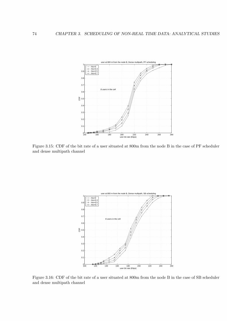
3.15 CDF of the bit rate of a user situated at 800m from the node B in the case of PF scheduler
and dense multipath channel . . . . . . . . . . . . . . . . . . . . . . . . . . . . . . . . . 74
3.16 CDF of the bit rate of a user situated at 800m from the node B in the case of SB scheduler
and dense multipath channel . . . . . . . . . . . . . . . . . . . . . . . . . . . . . . . . . 74
3.17 CDF of the bit rate of a user situated at 200m from the node B in the case of Max C/I
scheduler and Rayleigh fast fading . . . . . . . . . . . . . . . . . . . . . . . . . . . . . . 75
3.18 CDF of the bit rate of a user situated at 200m from the node B in the case of RR scheduler
and Rayleigh fast fading . . . . . . . . . . . . . . . . . . . . . . . . . . . . . . . . . . . . 76
3.19 CDF of the bit rate of a user situated at 200m from the node B in the case of PF scheduler
and Rayleigh fast fading . . . . . . . . . . . . . . . . . . . . . . . . . . . . . . . . . . . . 76
3.20 CDF of the bit rate of a user situated at 200m from the node B in the case of SB scheduler
and Rayleigh fast fading . . . . . . . . . . . . . . . . . . . . . . . . . . . . . . . . . . . . 77
3.21 Comparison between user the bit rates obtained by analytical model and simulation for
various schedulers and Rayleigh fast fading . . . . . . . . . . . . . . . . . . . . . . . . . 77
3.22 Comparison between user bit rates obtained by analytical model and simulation for var-
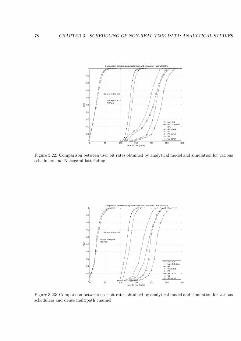
ious schedulers and Nakagami fast fading . . . . . . . . . . . . . . . . . . . . . . . . . . 78
3.23 Comparison between user bit rates obtained by analytical model and simulation for var-
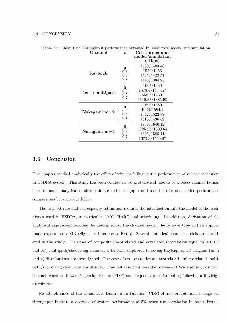
ious schedulers and dense multipath channel . . . . . . . . . . . . . . . . . . . . . . . . . 78
4.1 HENRI straight line of cdf−1(f) according to normal cdf−1 when the CS users number
is 10 . . . . . . . . . . . . . . . . . . . . . . . . . . . . . . . . . . . . . . . . . . . . . . . 90
4.2 percentage of speech and speech and LCD (Low Constraint Data) users (70% speech,
10% 32kbps, 10% 64kbps, 10% 128kbps) in soft handover according to the soft handover
margin (MSH) . . . . . . . . . . . . . . . . . . . . . . . . . . . . . . . . . . . . . . . . . 94
Page 22
LIST OF FIGURES xxi
4.3 Average cell throughput of HSDPA according to the number of speech and LCD (Low
Constraint Data) users (70% speech, 10% 32kbps, 10% 64kbps, 10% 128kbps) in the cell
in the presence of PF scheduling and Rayleigh fading channel . . . . . . . . . . . . . . . 106
4.4 Average cell throughput of HSDPA according to the number of speech and LCD (Low
Constraint Data) users (70% speech, 10% 32kbps, 10% 64kbps, 10% 128kbps) in the cell
in the presence of PF scheduling and dense multipath channel . . . . . . . . . . . . . . . 107
4.5 Average cell throughput of HSDPA according to the number of speech and LCD (Low
Constraint Data) users (70% speech, 10% 32kbps, 10% 64kbps, 10% 128kbps) in the cell
in the presence of PF scheduling and Nakagami (m=2) fading channel . . . . . . . . . . 107
4.6 Average cell throughput of HSDPA according to the soft handover margin (MSH) of
speech users in the cell in the presence of PF scheduling and Rayleigh fading channel . . 108
4.7 Average cell throughput of HSDPA according to the soft handover margin (MSH) of CS
(70% speech, 10% 32kbps, 10% 64kbps, 10% 128kbps) users in the cell in the presence of
PF scheduling and Nakagami fading channel . . . . . . . . . . . . . . . . . . . . . . . . . 108
4.8 CDF of the bit rate of a user situated at 800m from the node B in the case of PF
scheduling, Rayleigh fading channel, 40 speech users in the cell and MSH=3dB . . . . . 109
4.9 CDF of the bit rate of a user situated at 800m from the node B in the case of PF
scheduling, dense multipath channel, 40 speech users in the cell and MSH=3dB . . . . . 109
4.10 CDF of the bit rate of a user situated at 800m from the node B in the case of PF
scheduling, Nakagami fading channel, 40 speech users in the cell and MSH=3dB . . . . 110
5.1 CDF of user bit rate at the TCP level for user at 200m when the proportional fair
scheduler is used, in the presence of Rayleigh fading channel with rho=0, 0.5 . . . . . . 123
5.2 CDF of user bit rate at the TCP level for user at 800m when the proportional fair
scheduler is used, in the presence of Rayleigh fading channel with rho=0, 0.5 . . . . . . 123
5.3 HSDPA cell throughput at the TCP level when the proportional fair scheduler is used . 124
5.4 CDF of user bit rate at the TCP level for user at 200m when the proportional fair
and modified proportional fair are used, in the presence of Rayleigh fading channel with
rho=0, 0.5 . . . . . . . . . . . . . . . . . . . . . . . . . . . . . . . . . . . . . . . . . . . . 125
5.5 CDF of user bit rate at the TCP level for user at 800m when the proportional fair
and modified proportional fair are used, in the presence of Rayleigh fading channel with
rho=0, 0.5 . . . . . . . . . . . . . . . . . . . . . . . . . . . . . . . . . . . . . . . . . . . . 126
Page 23
xxii LIST OF FIGURES
5.6 Improvement of the HSDPA cell throughput at the TCP level when the modified propor-
tional fair scheduler is used . . . . . . . . . . . . . . . . . . . . . . . . . . . . . . . . . . 126
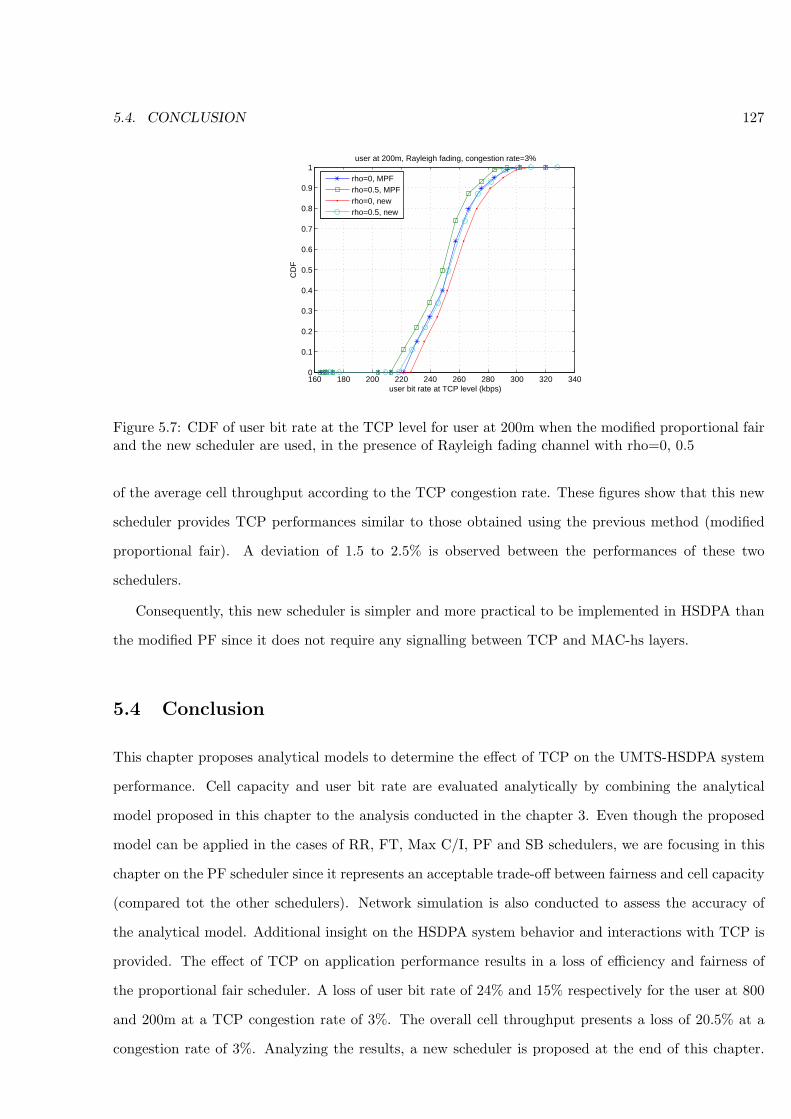
5.7 CDF of user bit rate at the TCP level for user at 200m when the modified proportional
fair and the new scheduler are used, in the presence of Rayleigh fading channel with
rho=0, 0.5 . . . . . . . . . . . . . . . . . . . . . . . . . . . . . . . . . . . . . . . . . . . . 127
5.8 CDF of user bit rate at the TCP level for user at 800m when the modified proportional
fair and the new scheduler are used, in the presence of Rayleigh fading channel with
rho=0, 0.5 . . . . . . . . . . . . . . . . . . . . . . . . . . . . . . . . . . . . . . . . . . . . 128
5.9 HSDPA cell throughput at the TCP level when the modified proportional fair and the
new scheduler are used . . . . . . . . . . . . . . . . . . . . . . . . . . . . . . . . . . . . . 128
6.1 CDF of the bit rate over 5 sec of a user situated at 200m from the node B in the case of
PF scheduler, 11 users in the cell . . . . . . . . . . . . . . . . . . . . . . . . . . . . . . . 143
6.2 CDF of the bit rate over 5 sec of a user situated at 800m from the node B in the case of
PF scheduler, 11 users in the cell . . . . . . . . . . . . . . . . . . . . . . . . . . . . . . . 143
6.3 CDF of the bit rate over 5 sec of a user situated at 800m from the node B in the case of
PF scheduler, 12 users in the cell . . . . . . . . . . . . . . . . . . . . . . . . . . . . . . . 144
6.4 CDF of the bit rate over 5 sec of a user situated at 200m from the node B in the case of
the scheduler proposed in [], 13 users in the cell . . . . . . . . . . . . . . . . . . . . . . . 144
6.5 CDF of the bit rate over 5 sec of a user situated at 800m from the node B in the case of
the scheduler proposed in [], 13 users in the cell . . . . . . . . . . . . . . . . . . . . . . . 145
6.6 CDF of the bit rate over 5 sec of a user situated at 800m from the node B in the case of
the scheduler proposed in [], 14 users in the cell . . . . . . . . . . . . . . . . . . . . . . . 145
6.7 CDF of the bit rate over 5 sec of a user situated at 200m from the node B in the case of
our proposed scheduler, 14 users in the cell . . . . . . . . . . . . . . . . . . . . . . . . . 146
6.8 CDF of the bit rate over 5 sec of a user situated at 800m from the node B in the case of
our proposed scheduler, 14 users in the cell . . . . . . . . . . . . . . . . . . . . . . . . . 146
6.9 CDF of the bit rate over 5 sec of a user situated at 800m from the node B in the case of
our propose scheduler, 15 users in the cell . . . . . . . . . . . . . . . . . . . . . . . . . . 147
Page 24
List of Tables
3.1 Mean Max C/I performance obtained by analytical model and simulation . . . . . . . . 79
3.2 Mean Round Robin performance obtained by analytical model and simulation . . . . . . 79
3.3 Mean Proportional Fair performance obtained by analytical model and simulation . . . 80
3.4 Mean Score Based performance obtained by analytical model and simulation . . . . . . 80
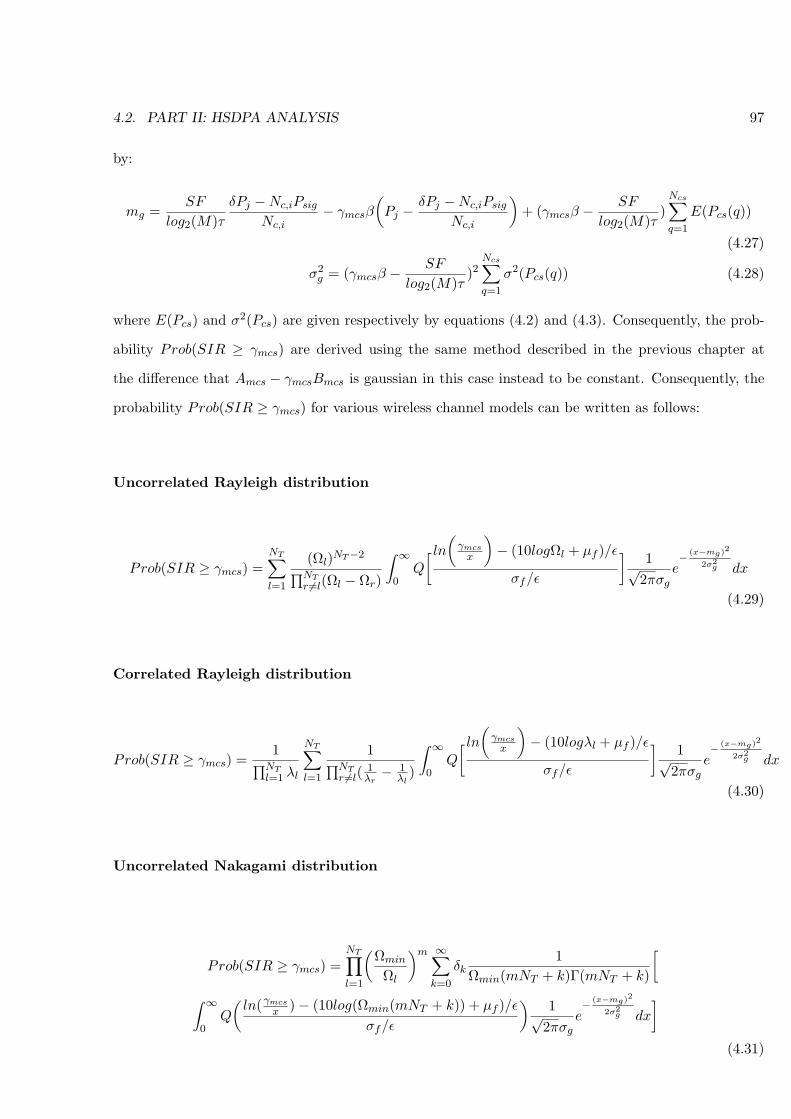
3.5 Mean Fair Throughput performance obtained by analytical model and simulation . . . . 81
1
Page 26
Chapter 1
General Introduction and Thesis
Contribution
1.1 General Introduction
The increased use of Internet and data services motivated the evolution of cellular systems from second to
third generation. The UMTS system (Universal Mobile for Telecommunications System) in Europe has
prepared for this evolution in successive releases within the third generation partnership project (3GPP)
that standardizes and specifies the UMTS air interface, the access and core network architectures.
Various advanced radio technologies are being introduced through the various releases in order to
convey mass market multimedia services in UMTS networks.
Release 99 of UMTS, the first release, relies mostly on the introduction of CDMA based radio and
access technologies. This step in the evolution remains insufficient to achieve full compatibility with
IP. The air interface as specified in release 99 does not provide the needed higher data rates either.
Therefore, releases 5 and 6 introduce a number of additional enhancements into the standard to enable
flexible and adaptive packet transmissions and to offer Internet based services.
HSDPA (High Speed Downlink Packet Access) is the umbrella of these evolutions on the downlink.
HSDPA has been introduced in the standards essentially in release 5. Release 6 contains some enhance-
ments to this technology in order to improve performance. The major introduced evolutions are at the
physical and data link layers.
The techniques introduced in HSDPA are adaptive modulation and coding (AMC) to achieve better
spectral efficiency, link adaptation to mitigate radio channel impairments, Hybrid ARQ (Automatic
3
Page 27
4 CHAPTER 1. GENERAL INTRODUCTION AND THESIS CONTRIBUTION
Repeat Request) to retransmit erroneously received radio blocs and to increase link reliability and
scheduling to enable intelligent allocation of resources to improve capacity and offer packet based mul-
timedia services. Scheduling over shared channels must take into account radio channel conditions,
mobile location in the cell and service type to provide tangible throughput, capacity and delay benefits.
Scheduling must also ensure fairness with respect to users and applications.
At the data link layer (Radio Link Control and Medium Access Control) and the radio resource
control, another major enhancement was the addition of the downlink shared channels next to the release
99 dedicated channels. The dedicated channels are suitable for real time services but are inadequate for
packet services. The introduction of shared channels results in power savings, interference mitigation
and system capacity improvements.
Besides, Multiple transmit and receive antennas can also be used to achieve higher data rates and
improve system capacity. The introduction of multiple antennas is planned for the last phases of the
UMTS architecture enhancements.
The introduction of new features in networks to improve data rates and enhance reliability of data
transmission over the air interface can have nevertheless an impact on end to end performance and
efficiency. Retransmission mechanisms relying on ARQ interact with higher layer protocols, especially
the Transport Control Protocol (TCP) used in conjunction with IP to offer non real time services. Real
time services are typically offered using UDP/IP and streaming services using RTSP/RTP/IP. Cross
layer interactions can have a drastic impact on overall throughput and capacity. Care must be taken to
characterize these interactions and suggest ways of preventing or at least reducing any negative effects
resulting from the introduction of ARQ and other techniques in wireless networks that unavoidably
interact with congestion control mechanisms in Internet networks (when TCP protocol is used) and
generate additional delay in receiving data which can affect the efficiency of HSDPA for services with
stringent delay constraints (e.g., streaming).
1.2 Thesis Objectives
This thesis focuses on the analysis and modeling of cross layer interaction between the new MAC-hs
(MAC high speed) of HSDPA system and other layers (physical, transport and application layers). The
objective is to find the best configuration of this layer to minimize the negative interaction between
layers and optimize the performance of HSDPA. The studies in this thesis are conducted to answer the
following objectives:
Page 28
1.2. THESIS OBJECTIVES 5
• Characterize the effect of wireless channel (shadowing, fast fading,..) on the performance of
HSDPA. The Adaptive Modulation and coding, fast link adaptation and fast scheduling techniques
introduced in HSDPA are tightly coupled to adapt the transmission parameters to the continuous
varying channel and optimize the resource management by allocating the HS-DSCH channel to
the user having favorable channel conditions. In this context, the channel variations (especially
short term variations) have an important impact on the efficiency of the system performance.
To the best of our knowledge, this topic has not been studied yet in the literature. Therefore,
the first objective of this thesis is to model analytically the effect of the wireless channel on
the performance of the HSDPA system. Several channel models are considered (Rayleigh fading
channel, Nakagami fading channel,..). Results obtained from this analysis are of interest to assess
the efficiency of the schedulers used in HSDPA and the impact of the wireless environment on the
HSDPA performance.
• Characterize the interaction between the MAC-hs and the data link layer of the UMTS R99
(Release 99). Since HSDPA has been conceived for packet switched services, the UMTS R99 will
still be used, in parallel to HSDPA, to convey speech and circuit switched services. The interaction
between these two service classes that use the same wireless bandwidth and CDMA code tree must
be assessed to determine the impact of the UMTS R99 capacity on the HSDPA capacity. This
topic has not been addressed in the literature. The challenge consists not only in characterizing
this interaction between R99 services and HSDPA connections but also in modeling analytically
this interaction for various schedulers used in HSDPA and various wireless fading channel models.
• Characterize analytically the interaction between the MAC-hs layer and the Transport Control
Protocol (TCP). As described herein, the introduction of new features in HSDPA such as Hybrid
ARQ and fast scheduling unavoidably interact with congestion control mechanisms in the Inter-
net. TCP misinterprets the delay generated by HARQ and scheduling techniques and triggers
unnecessary timeout mechanisms resulting in congestion window shrinking and drastic through-
put degradation. The challenge in this case is to characterize analytically these interactions and
suggest ways of preventing or at least reducing any negative effects to improve the performance
of TCP over HSDPA (e.g., introduce of a new scheduler that reduces these negative interactions).
Although the performance of TCP over wireless networks has been studied widely in the liter-
ature, few studies are conducted in the case of HSDPA. These studies are essentially based on
Page 29
6 CHAPTER 1. GENERAL INTRODUCTION AND THESIS CONTRIBUTION
simulation. Moreover, the majority of studies on TCP over wireless systems propose modification
of TCP implementations which is not desirable. Relying on scheduling to minimize interactions of
lower layer protocols with TCP and achieve capacity benefits without breaking the IP paradigm
is a more appropriate alternative.
• Characterize the interaction between the MAC-hs layer and the streaming Quality of Service (QoS)
constraints. Streaming is one of the emerging services that are expected to occupy a large share
of the wireless system capacity. Streaming services are characterized by stringent QoS constraints
(delay, jitter,...). Transmitting the streaming services over shared channels using the existing
schedulers results in cell throughput degradation due to the jitter constraints. Consequently,
characterizing the interaction of streaming services with the MAC-hs is needed to conceive an
appropriate scheduler to convey these services over HSDPA without losing much cell capacity.
The challenge in this case is to design an opportunistic scheduler achieving a trade-off between
fairness and cell capacity, in other words guaranteeing the required streaming QoS constraints
without losing much cell capacity. Few studies on this topic are available in the literature.
1.3 Thesis Contributions
The contributions of this thesis can be classified into four major analyses that mirror the challenges
described earlier on the effect of the environment, of other protocols and other UMTS channels on the
HSDPA system capacity:
• Effect of radio channel models on HSDPA performance (chapter 3);
• Interaction of HSDPA services with R99 Circuit Switched services transmitted (chapter 4);
• Interaction of MAC-hs and schedulers with TCP protocol (chapter 5);
• Interaction of MAC-hs and schedulers with Streaming services (chapter 6).
These studies are conducted using analytical and statistical analysis. A network system simulation is
also used to assess the accuracy of the proposed models. In the fourth contribution, only a fraction of
the proposed solutions and simulation results is reported in this thesis. Other contributions related to
a research contract are not reported for confidential reasons.
Chapter 2 provides background information on the HSDPA system to introduce the context of the
conducted studies in this thesis.
Page 30
1.3. THESIS CONTRIBUTIONS 7
Chapter 7 concludes the manuscript by summarizing the studies and presents perspectives to pursue
and extend the thesis.
1.3.1 Effect of radio channel models on HSDPA performance (chapter 3)
As indicated above, HSDPA relies on several advanced technologies such as AMC, HARQ and scheduling
to improve the system capacity and allow the introduction of new high bit rate services. These techniques
are tightly coupled and benefit from the shared time nature of the transport channel (the so-called HS-
DSCH) to allocate the HS-DSCH channel to the adequate user at the right moment and to adapt
its transmission parameters to the short term radio channel variations. In this context, the role of the
scheduling is essential for the improvement of system efficiency and performance. The scheduling should
maximize as much as possible the cell throughput and offer to each user enough resources to achieve
the desired Quality of Service (QoS) for each application. Consequently, the efficiency of the scheduler
depends essentially upon the conveyed traffic characteristics and the wireless channel model. A cross
layer study between the wireless channel (modeled by path loss, shadowing, fast fading, correlation
between channel paths,...), the MAC-hs layer (HARQ, AMC, scheduling) and the application QoS
constraints is essential to estimate the performance of HSDPA, find a good configuration of the MAC-
hs (find a good scheduler,...) and optimize the planning of the HSDPA system.
This thesis studied analytically the effect of wireless fading on the performance of various schedulers
in HSDPA. This study has been conducted using statistical models of the wireless channel fading.
The proposed analytical models estimate cell throughput and user bit rate and enable performance
comparisons between schedulers.
The user bit rate and cell capacity estimation requires the introduction into the model of the tech-
niques used in HSDPA, in particular AMC, HARQ and scheduling. In addition, derivation of the
analytical expressions requires the description of the channel model, the receiver type and an approxi-
mate expression of SIR (Signal to Interference Ratio). Several statistical channel models are considered
in the study. The cases of composite uncorrelated and correlated multipath/shadowing channels with
path amplitude following Rayleigh and Nakagami distributions are investigated. The case of composite
dense uncorrelated and correlated multipath/shadowing channel is also studied. This last case consid-
ers a Wide-sense Stationary channel, constant Power Dispersion Profile (PDP) and frequency selective
fading following a Rayleigh distribution.
Finally, results obtained from the analytical models are verified by a system simulation conducted
Page 31
8 CHAPTER 1. GENERAL INTRODUCTION AND THESIS CONTRIBUTION
using the Network Simulator NS2. Note that the conducted studies in this part of the thesis assume
the use of non real time data in particular FTP traffic.
1.3.2 Interaction of HSDPA services with Circuit Switched services transmitted on
UMTS R99 dedicated channels (chapter 4)
Since HS-DSCH is reserved only for non real time data services, CS services will be transmitted as
before on downlink dedicated channels known as DPCH channels (Dedicated Physical Channel). The
DPCH channel, normalized by the 3GGP in Release 99, supports fast power control and soft handover.
In the case of multiple services, policies to set priorities between the various services are required to
achieve adequate throughput and service differentiation and to offer each service their required bit rate
and QoS. The scenario of interest in this part of the thesis corresponds to the simultaneous presence
of circuit switched (CS) services (e.g., speech) on the DPCH channel and of HSDPA packet services on
the HS-DSCH channel. The priority between CS users and HSDPA users can be found by analyzing the
effect that CS services have on the capacity of HSDPA. To assess interaction between CS and HSDPA
packet services, an analytical model is proposed to estimate the capacity of HSDPA in the presence of
CS users on the DPCH channels. A network level simulation, implemented in NS-2, is used to evaluate
the accuracy of the proposed model.
CS services consume part of the code tree resources and the node B power and exert interference on
the HSDPA packet services. The entire left over node B power is used to serve HSDPA packet services.
Estimating, approximating or lower bounding the capacity of the HSDPA system requires prior analysis
of CS services. The basic analytical expression for HSDPA capacity includes terms related to HARQ,
fast scheduling and the selected AMC combination according to radio link conditions. Consequently,
the derivation of the analytical model requires prior assessment of CS services behavior in terms of total
power consumption (including soft handover aspects), the relationship that exists between codes used
by CS services and those left for HSDPA users, the scheduling used and the ensuing AMC combination
for HSDPA users. The derivation of the analytical model proposed in the contribution to estimate the
capacity of HSDPA considers as in the previous analyses (presented above i.e. without the presence
of CS services) several scheduling algorithms under various wireless channel model (cases of composite
uncorrelated and correlated multipath/shadowing channels with path amplitude following Rayleigh
and Nakagami distributions, case of composite dense uncorrelated and correlated multipath/shadowing
channel with Wide-sense Stationary channel, constant Power Dispersion Profile (PDP) and frequency
Page 32
1.3. THESIS CONTRIBUTIONS 9
selective fading following a Rayleigh distribution).
The accuracy of the obtained results are also assessed by a system simulation using NS2.
1.3.3 Interaction of MAC-hs and schedulers with the TCP protocol (chapter 5)
The interaction between radio link control mechanisms and TCP has been identified early in the scientific
community that has since provided many variants for TCP to reduce and possibly eliminate interactions
when random errors over the air interface are mistakenly taken by TCP as congestion in the fixed network
segments. Even if some approaches propose link layer solutions, most tend to break the end to end IP
paradigm when TCP is modified in an attempt to alleviate the experienced negative cross layer effects
due to errors occurring over the radio link. Among the proposed solutions, only a few are actually used
in practice. Split TCP has been used in public land mobile networks (PLMNs) at gateways located
at the edge of wireless core networks to separate the Internet from the PLMNs and thereby avoiding
interactions between TCP and the radio link errors and recovery mechanisms. Some TCP versions have
also become de facto standards because they have been extensively deployed in the Internet during the
quest for alternatives to the standard or the original TCP. This thesis will consequently focus on the
more common and popular versions of TCP (TCP Reno) to conduct the analysis of interactions between
Hybrid ARQ, scheduling and TCP congestion mechanism. In addition, this thesis goes further as it
clearly contends that systems using scheduling over the air interface are better off taking advantage
of scheduling itself to alleviate the RLC/TCP interactions rather than violating the end to end IP
paradigm. An analytical model is proposed to assess the cell throughput for HSDPA using several
scheduling algorithms and the de facto TCP Reno congestion control algorithm. The results reported
in chapter 5 indicate that wireless systems can rely on scheduling to minimize interactions of lower layer
protocols with TCP and achieve capacity benefits without breaking the IP paradigm. An analytical
expression of cell throughput provides insight on capacity behavior. A new scheduler has been proposed
in this part of the thesis (chapter 5) to improve the performance of TCP over the HSDPA system and
minimize the negative interaction between TCP and the reliable data link layer.
1.3.4 Interaction of MAC-hs and schedulers with Streaming services (chapter 6)
Streaming applications are supposed to occupy a large share of the third generation system bandwidth.
The fundamental characteristic of this application class is to maintain traffic jitter under a specific
threshold. Jitter relates to the time relation between received packets. This threshold depends on the
Page 33
10 CHAPTER 1. GENERAL INTRODUCTION AND THESIS CONTRIBUTION
application, the bit rate and the buffering capabilities at the receiver. The use of a buffer at the receiver
smoothes traffic jitter and reduces the delay sensitivity of the application.
In this thesis, we have conducted a study on the scheduling algorithms for streaming services in
the UMTS HSDPA system. The objective is to see if basic scheduling algorithms are suitable for
streaming services. In other words, can these algorithms achieve an acceptable cell capacity while
offering streaming services with fixed reading rates (i.e. Constant Bit Rate or CBR typically at target
bit rate of 128kbps). Selected sources in the analysis operate consequently at 128 kbps as CBR streaming
traffic. The entire end to end path from the applications in the User Equipment (UE) to the source
side (in the network) is considered.
This study has been conducted in the context of a research project with France Telecom Research
and Development (FTR&D). Consequently, only a fraction of the proposed schedulers and results will
be reported in this public document. The results in this manuscript correspond to presence of composite
uncorrelated multipath/shadowing channel with amplitude following a Rayleigh distribution.
Results show that basic schedulers (e.g., Proportional Fair,...) are not suitable for streaming traffic.
The bit rate fluctuations over time do not allow offering streaming services with acceptable cell capacity.
At the end of this thesis, a new scheduler, more appropriate for handling streaming services, has been
consequently suggested to alleviate the weaknesses observed and encountered for the basic schedulers.
Simulations assess the performance of this new scheduler and show that it can outperform other existing
schedulers in terms of capacity and fairness.
Page 34
Chapter 2
High Speed Downlink Packet Access
(HSDPA)
The UMTS system proposed for third generation cellular networks in Europe, is meant to provide
enhanced spectral efficiency and data rates over the air interface. The objective for UMTS, known
as WCDMA in Europe and Japan, is to support data rates up to 2Mbps in indoor/small-cell-outdoor
environments and up to 384 Kbps in wide-area coverage for both packet data and circuit-switched data.
The 3GPP, responsible for standardizing the UMTS system, realized early on that the first releases
for UMTS would be unable to fulfill this objective. This was evidenced by the limited achievable bit
rates and aggregate cell capacity in release 99. The original agenda and schedule for UMTS evolution
has been modified to meet these goals by gradual introduction of advanced radio, access and core
network technologies through multiple releases of the standard. This phased roll out of UMTS networks
and services would also ease the transition from second generation to third generation cellular for
manufacturers, network and service providers. To meet in addition the rapidly growing needs in wireless
Internet applications, studies initiated by 3GPP since 2000 not only anticipated this needed evolution
but also focused on enhancements of the WCDMA air interface beyond the perceived third generation
requirements.
The High Speed Downlink Packet Access (HSDPA) system [1-5] has been proposed as one of the
possible long term enhancements of the UMTS standard for downlink transmission. It has been adopted
by the 3GPP and will be used in Europe starting in 2006/2007. HSDPA introduces, first, adaptive
modulation and coding, retransmission mechanisms over the radio link and fast packet scheduling and,
later on, multiple transmit and receive antennas. This chapter describes the HSDPA system and some
11
Page 35
12 CHAPTER 2. HIGH SPEED DOWNLINK PACKET ACCESS (HSDPA)
of these related advanced radio techniques. Once the multiple antenna systems envisaged in HDSPA
are integrated, UMTS networks will be able to achieve aggregate cell throughput in the 10 to 20 Mbps
range.
2.1 HSDPA Concept
Interference control and management is key in increasing cell capacity in CDMA based systems. This
can be performed at the link level by enhanced receiver structures such as Multi User Detection (MUD)
used to minimize the level of interference at the receiver. At the network level, a good management of
the interference can be provided by an enhanced power control and associated Call Admission Control
(CAC) algorithms.
This philosophy of simultaneously managing the interference at the network level for dedicated
channels leads to limited system efficiency. Fast power control used to manage the interference increases
the transmission power during the received signal fades. This causes peaks in the transmission power
and subsequent power rises that reduce the total network capacity. Power control imposes provision of
a certain ”headroom” or margin in the total Node B transmission power to accommodate variations [6].
Consequently, system capacity remains insufficient and unable to respond to the growing need in bit
rates due to the emergence of Internet applications. A number of performance enhancing technologies
must be included in the UMTS standard to achieve higher aggregate bit rates in the downlink and to
increase the spectral efficiency of the entire system. These techniques include Adaptive Modulation
and Coding (AMC), fast link adaptation, Hybrid ARQ and fast scheduling. Multi User Detection
(MUD) and Multiple Input Multiple Output (MIMO) antenna solutions can also be included, but this
is expected in later releases of UMTS to further improve system performance and efficiency.
The use of higher order modulation and coding increases the bit rate of each user but requires
more energy to maintain decoding performance at the receiver. Hence, the introduction of fast link
adaptation is essential to extract any benefit from introducing higher order modulation and coding in
the system. The standard link adaptation used in current wireless system is power control. However,
to avoid power rise as well as cell transmission power headroom requirements, other link adaptation
mechanisms to adapt the transmitted signal parameters to the continuously varying channel conditions
must be included. One approach is to tightly couple AMC and Scheduling. Link adaptation to radio
channel conditions is the baseline philosophy in HSDPA which serves users having favorable channel
conditions. Users with bad channel conditions should wait for improved conditions to be served. HSDPA
Page 36
2.1. HSDPA CONCEPT 13
adapts in parallel the modulation and the coding rates according to the instantaneous channel quality
experienced by each user.
AMC still result in errors due to channel variations during packet transmission and feedback-delays
in receiving channel quality measurements. A Hybrid-ARQ scheme can be used to recover from link
adaptation errors. With Hybrid-ARQ, erroneous transmissions of the same information block can
be combined with subsequent retransmission before decoding. By combining the minimum number
of packets needed to overcome the channel conditions, the receiver minimizes the delay required to
decode a given packet. There are three main schemes for implementing HARQ : Chase combining
(retransmissions are a simple repeat of the entire coded packet), Incremental redundancy IR (additional
redundant information is incrementally transmitted) and self decodable IR(additional information is
incrementally transmitted but each transmission or retransmission is self decodable).
The link adaptation concept adopted in HSDPA implies the use of time shared channels. Therefore,
scheduling techniques are needed to optimize the channel allocation to the users. Scheduling is a key
feature in the HSDPA concept and is tightly coupled to fast link adaptation. Note that the time-shared
nature of the channel used in HSDPA provides significant trunking benefits over DCH for bursty high
data rate traffic.
The HSDPA shared channel does not support soft handover due to the complexity of synchronizing
the transmission from various cells. Fast cell selection can be used in this case to replace the soft han-
dover. It could be advantageous to be able to rapidly select the cell with the best Signal to Interference
Ratio (SIR) for the downlink transmission.
HSDPA can be seen as ”an umbrella of enhancement techniques applied on a combined CDMA-
TDMA (Time Division Multiple Access) channel shared by users” [6]. This channel, called High Speed
Downlink Shared Channel (HS-DSCH), is divided into slots called Transmit Time Intervals (TTIs) each
one equal to 2ms. The signal transmitted during each TTI uses the CDMA technique. Since link
adaptation is used, the variable spreading factor is deactivated because its long-term adjustment to the
average propagation conditions is not required anymore. Therefore, the spreading factor is fixed and
equal to 16. The use of relatively low spreading factor addresses the provision for increased applications
bit rates.
Finally, the transmission of multiple spreading codes is also used in the link adaptation process.
However, a limited number of Wash codes is used due the low spreading adopted in the system. Since
all these codes are allocated in general to the same user, Multi User Detector (MUD) can be used at the
Page 37
14 CHAPTER 2. HIGH SPEED DOWNLINK PACKET ACCESS (HSDPA)
User Equipment (UE)to reduce the interference between spreading codes and to increase the achieved
data rate. This is in contrast to traditional CDMA systems where MUD techniques are used in the
uplink only.
2.2 Channels Structure
HSDPA consists of a time shared channel between users and is consequently suitable for bursty data
traffic. HSDPA is basically conceived for non real time data traffic. Research is actually ongoing to
handle streaming traffic over HSDPA using improved scheduling techniques.
In addition to the shared data channel, two associated channels, called High Speed Shared Control
Channel (HS-SCCH) and High Speed Dedicated Physical Control Channel (HS-DPCCH), are used in
the downlink and the uplink to transmit signalling information to and from the user. These three
channels in HSDPA : HS-DSCH, HS-SCCH and HS-DPCCH are described in more details.
2.2.1 HS-DSCH Channel
The fast adaptation to the short term channel variations requires handling of fast link adaptation at
the node B. Therefore, the data transport channel HS-DSCH is terminated at the node B. This channel
is mapped onto a pool of physical channels called High Speed Physical Downlink Shared Channel (HS-
PDSCH) to be shared among all the HSDPA users on a time and code multiplexed manner [7, 8].
Each physical channel uses one channelization code, of fixed spreading factor equal to 16, from the
set of 15 spreading codes reserved for HS-DSCH transmission. Multi-code transmission is allowed,
which translates to mobile user being assigned multiple codes in the same TTI, depending on the User
Equipment (UE) capability. Moreover, the scheduler may apply code multiplexing by transmitting
separate HS-PDSCHs to different users in the same TTI.
The transport channel coding structure is reproduced as follows: One transport block is allocated per
TTI, so that no transport block concatenation (such as in UMTS DCH based transmission) is used. The
size of transport block changes according to the Modulation and Coding Scheme (MCS) selected using
the Adaptive Modulation and Coding (AMC) technique. To each transport block, a Cyclic Redundancy
Check (CRC) sequence with 24 bits is added. Since errors occur in bursts, one CRC sequence per
transport block (i.e. per TTI) is sufficient. Once the CRC sequence is attached, the transport block
bits are bit scrambled and segmented into blocks to apply Turbo block encoding. The code block size
depends upon the turbo coding rate and can reach a maximum value of 5114 bits [9]. The coding
Page 38
2.2. CHANNELS STRUCTURE 15
rate changes according to the MCS scheme selected by the link adaptation technique. At the turbo
encoder output, rate matching is applied by the physical layer HARQ functionality. After matching the
number of bits to the number of bits in the allocated HS-DSCH physical channels, segmentation divides
the resulting bits among the HS-DSCH physical channels. The bit sequence obtained for each physical
channel is then interleaved using one step interleaver with fixed size 32×30 (i.e. 32 rows and 30 columns)
[9]. Finally, the resulting bit sequence is modulated using 16-ary Quadrature Amplitude Modulation
(16QAM) or Quadrature Phase Shift Keying (QPSK) according to the MCS scheme selected [10,11].
2.2.2 HS-SCCH Channel
The downlink signalling related to the HS-DSCH is transmitted over the High Speed Shared Control
Channel (HS-SCCH). The signalling information carried by the HS-SCCH contains essentially the Trans-
port Format Resource Indicator (TFRI) and the HARQ information of the HS-DSCH channel. The
TFRI includes the channelization codes used by the HS-DSCH, the modulation scheme and the trans-
port block size. The HARQ information consists of the HARQ new data indicator, the HARQ process
identifier and the redundancy and constellation version. Since the HS-DSCH channel is shared among
users, the UE Identity (ID) is sent over the HS-SCCH to indicate the identity of the user for which the
HS-DSCH is allocated during the TTI. Note that the UE ID is given by the 16 bits HS-DSCH Radio
Network Temporary Identifier (H-RNTI) defined by the Radio Resource Controller (RRC) [12, 13].
Finally, this channel can be transmitted at a fixed power or can use power control. The decision to
use power control is entirely left to the implementation.
2.2.3 HS-DPCCH Channel
In the uplink, signalling information has to be transmitted for the HARQ acknowledgment and the
feedback measurement. The use of fast link adaptation on the HS-DSCH channel requires knowledge
of the channel quality during the transmission. The UE measures the channel quality on the Common
Pilot Indicator Channel (CPICH) and sends the result to the node B. The use of HARQ requires an
acknowledgment message from the user to the node B, so that the node B retransmits the erroneously
received packet or a new packet.
This signalling information is carried by the HS-DSCH associated uplink dedicated control channel
(HS-DPCCH). This channel is spread, with a spreading factor of 256 (i.e. 30 bits per TTI), and code
multiplexed with the existing dedicated uplink physical channels (DPCH). The H-ARQ acknowledgment
Page 39
16 CHAPTER 2. HIGH SPEED DOWNLINK PACKET ACCESS (HSDPA)
is a 1-bit Ack/Nack indication repeated 10 times and transmitted in one slot. The H-ARQ acknowl-
edgement field is gated off when there is no ACK/NACK information being sent. The measurement
feedback information contains Channel Quality Indicator (CQI) that may be used to select transport
format and resource by HS-DSCH serving Node-B, according to CQI tables specified in [11]. It is an
essential information needed for fast link adaptation and scheduling. The channel quality information,
consisting of 5 bits, is coded using a (20,5) code transmitted over two slots.
2.3 MAC-hs
The use of fast adaptation to the short term channel variations requires handling of the HSDPA transport
channels by the node B. Therefore, a Medium Access Control-high speed (MAC-hs) entity has been
introduced in the node B. This entity has the responsibility of handling the HARQ process, scheduling
and the selection of the transport format (due to AMC) [14]. The MAC-hs also stores the user data
to be transmitted across the air interface. This imposes some constraints on the minimum buffering
capabilities of the Node B.
2.4 Fast Link Adaptation
The wireless channel in cellular systems is a composite multipath/shadowing channel. The radio waves
follow several paths from the transmitter to reach the destination. Fading occurs when many paths
interfere, adding up to a composite signal exhibiting short time signal power variations at the receiver.
This power could be weaker or stronger than the required power needed to achieve a given user Quality
of Service (QoS). The link quality between the transmitter and the receiver is also affected by slow
variations of the received signal amplitude mean value due to shadowing from terrains, buildings, and
trees.
To deal with the problems caused by multipath fast fading, the existing wireless systems use diversity
techniques such as long interleaving, robust channel coding, frequency hopping, and direct sequence
spread spectrum. These techniques are based on one concept: averaging the temporary fading effect
over all the transmission time and the bandwidth, so that bad conditions are compensated by good
conditions. The spread spectrum technique (frequency hopping and direct sequence) spread the signal
bandwidth over a wider frequency spectrum so that only a part of the spectrum is affected by the fading.
Interleaving can be seen as spreading technique over time. By reordering the bits before transmission,
Page 40
2.4. FAST LINK ADAPTATION 17
the information message is spread out over time. Therefore, bursty errors caused by the fading channel
are spread out in time so the decoder receives distributed non bursty random errors that are easier
to detect and correct. The channel coding includes redundancy in the transmitted signal to increase
robustness against errors. Introducing more redundancy increases robustness but decreases effective
information bit rate. In current systems, the channel coding rate is fixed to deal with the worst case
and the transmission power is adapted to the channel conditions in order to achieve the application QoS
[15].
Since fading results from the addition of different waves from multiple paths, it can potentially be
predicted. Channel parameters (amplitude, phase, frequency), remain stationary for time windows of
the order of half a wavelength. For example, at a carrier frequency of 2GHz (case of UMTS) and a
mobile speed of 36 Km/h, the fading pattern could be predicted for a time window of approximately
7.5 ms. Estimation of the channel is feasible over a few ms and power can be consequently adjusted
over such time scales.
In the UMTS R99, channel estimation is used to adapt the transmission power of each user, every
slot (corresponding to a rate of 1500 Hz), to the short term channel variations. This is achieved at the
cost of some power rise and higher interference as previously explained in section 2.2.
In HSDPA, the idea is to avoid power adaptation and hence power control by approaching the radio
resource allocation and sharing from a different angle. Why continue using averaging techniques such as
long interleaving and a fixed channel coding rate to counteract the fast fading if these techniques require
high performance power control? Instead one can use AMC tightly coupled with fast scheduling so that
modulation orders and coding rates are adapted according to estimated channel fading. In addition,
the HS-DSCH channel can be allocated to the user with favorable channel conditions. To this avail, a
Channel Quality Indicator (CQI) has been introduced in HSDPA (for details, see next section)to enable
such intelligent allocation of resources to users.
The idea is to measure the channel quality over the Common Pilot Indicator Channel (CPICH) and
to transmit the measurement report over the HS-DPCCH channel to the node B, so that scheduling and
AMC can act according to the CQI and hence optimize channel resource allocation. The time window
between the channel conditions measurement and the resource allocation should not exceed half a
wavelength as indicated previously. In the 3GPP specifications [11], 30 CQIs have been standardized
as described in the next section. The time window between the channel measurement and the start of
the transmission over the HS-DSCH channel is 7 timeslots. By considering the transmission time of the
Page 41
18 CHAPTER 2. HIGH SPEED DOWNLINK PACKET ACCESS (HSDPA)
HS-DSCH channel (1 TTI), the overall delay between the radio channel measurement and the end of
the packet transmission over the HS-DSCH channel is 10 timeslots. Therefore, HSDPA is suitable for
urban area when mobile users move at low speed (less than 40 Km/h). For mobile at higher speeds,
the environment conditions change rapidly. ”Fortunately, in this case the mobiles have a low degree
of randomness since they move along known paths (traveling by train, driving down a freeway, etc..).
Therefore, special solutions can be performed to predict the channel fading pattern in these cases” [15].
In the 3GPP R6 (Release 6), enhancements are added to the CQI reporting method by introducing
tuneable reporting rates through additional CQI reports during periods of downlink activity and fewer
reports at other times [4]. These additional CQIs can be initiated on demand of fast layer 1 signalling.
In addition, a certain number of successive CQI values may be averaged with respect to channel quality
at the UE. The averaged value is reported and used with the instantaneous CQI measured to select the
Modulation and Coding Scheme (MCS). The motivation for this technology is to improve the selection
of MCS, so that the delay due to HARQ retransmissions can be reduced. In addition, the UL signalling
overhead may be reduced and this decreases the uplink interference. Finally, the use of the feature
requesting extra CQI transmissions by fast layer 1 signalling improves the performance of the first
packets of a packet call.
2.5 Adaptive Modulation and Coding
As explained earlier, the link adaptation in HSDPA is performed by the use of Adaptive Modulation and
Coding. According to the channel quality, the modulation and the coding assigned to the user change,
so that higher peak data rate and average throughput can be provided. A Channel Quality Indicator
(CQI) has been introduced to inform the system about the channel conditions. In order to guarantee
a Block Error Rate (BLER) greater than 10% on the HS-PDSCH, each CQI is mapped onto a specific
Modulation and Coding Scheme (MCS) corresponding to a given transport format. The selection of the
transport format is performed by the MAC-hs located in the node B. Each transport format or MCS is
defined by a [11]:
1. Modulation format, which can be either QPSK or 16QAM
2. Turbo encoder rate, which varies between 0.17 and 0.89. The encoding rate depends upon the User
Equipment (UE) capabilities (maximum number of HS-DSCH codes that the UE can handle) and
the desired Transport Block Size (TBS). The different code rates are obtained through puncturing
Page 42
2.6. HYBRID-ARQ 19
of bits in the turbo encoder of rate 1/3.
3. Number of HS-PDSCH codes allocated to the user, which ranges from 1 to the maximum number
of codes supported by the UE (depends on UE category). Note that for any UE category, this
number can not exceed 15 codes. In fact, the spreading factor used in HSDPA is fixed at 16.
Therefore, 16 branch codes are available from which at least one code branch is reserved for
signalling and control channels. Thus, leaving a maximum of 15 codes to allocate to a given user
at best.
In the 3GPP specifications [11], 12 UE categories are defined according to the maximum number of
HS-DSCH that the UE can handle simultaneously. The transport formats and the corresponding CQIs
for all UE categories can be found in [11].
2.6 Hybrid-ARQ
Fast link adaptation provides the flexibility to match the MCS to the short term channel variations for
each user. However, link adaptation is sensitive to measurement errors, delays in the CQI procedure and
unexpected channel variations. Therefore, the use of ARQ, which is insensitive to CQI measurement
errors, is indispensable to tolerate higher error rates in order to save cell resources, use higher order
MCS and increase the user and the average cell throughput.
The ARQ technique used in UMTS is Selective Repeat (SR). The retransmissions are performed
by the RLC layer in the RNC. Introducing ARQ induces delays in receiving error free information and
interacts unfortunately with higher layer protocols such as the Transmission Control Protocol (TCP)
used to handle end to end IP packcet communications between end hosts. If these interactions are
not addressed and handled properly, drastic degradation in applications flow rates will be experienced.
These interactions and means to reduce their negative effects on overall system throughput are addresses
in chapters 6 and 7.
In HSDPA, the ARQ protocol is performed by the MAC-hs entity in the node B. HSDPA uses the
ARQ protocol combined with Forward Error Correction (FEC) code so that an erroneous packet is not
discarded but softly combined with its retransmissions in order to reduce the average delay in receiving
error-free information. In addition, the tight coupling of Hybrid-ARQ and fast link adaptation limits
the excessive use of ARQ (in other words the delay) since retransmissions occur if link adaptation fails
to cope with the instantaneous channel conditions.
Page 43
20 CHAPTER 2. HIGH SPEED DOWNLINK PACKET ACCESS (HSDPA)
2.6.1 Hybrid-ARQ types
In HSDPA, three types of HARQ have been studied and standardized in the 3GPP specifications
[1,14,16-20]: Chase combining, Incremental Redundancy (IR) and self decodable IR.
In [17], D. Chase has shown that the sequence resulting of combining two copies of the same sequence
presents a lower error rate than the original sequences. Therefore, instead of discarding erroneous
packets, the UE proceeds to soft combining (called Chase combining) of multiple retransmissions of the
same packets before decoding. This concept, developed and standardized in the 3GPP specifications
(Release 5) [1], reduces the delays compared to the ARQ used in the UMTS R99. This HARQ algorithm
does not interact optimally with the AMC and the fast link adaptation since the multiple retransmissions
are the same copies of the first one, i.e. the same MCS is used even if the channel conditions change.
Consequently, enhanced HARQ algorithms have been introduced in the 3GPP specifications [1,14].
These new schemes rely on on Incremental redundancy (IR).
In HARQ IR, instead of retransmitting the same copy of the erroneous packet, redundant information
is incrementally added to retransmissions copies. This represents a better protection of the information
packets and copes more with channel conditions and AMC. In this type of HARQ, only a fraction of
the information sequence is sent in the retransmission packet (according to the redundancy degree).
The retransmitted packet is not self decodable and should be combined with the first transmission
before decoding. To counteract this problem, a IR scheme that is self decodable has been studied and
developed by the 3GPP [1,14]. To obtain a self decodable scheme, incremental redundant information is
added to the first sequence and incremental puncturing is also used so that the receiver can reconstruct
the information sequence and decode each retransmission before soft combining the retransmissions in
case of unsuccessful decoding.
2.6.2 HARQ Protocol
The increase in complexity and in requirements of the HARQ SR leads to the adoption of simpler
HARQ strategies. The Stop and Wait (SW) ARQ protocol is quite simple to implement but since it is
inefficiency, a trade-off between between the simple SW and the SR, called N-Channel SW, has been
developed and standardized for HSDPA [1,14].
The N-Channel SW consists of activating N HARQ processes in parallel, each one using the SW pro-
tocol. Hereby, one HARQ instance (process) can transmit data on the HS-DSCH while other instances
are waiting for the acknowledgment on the uplink. Using this strategy, the retransmission process be-
Page 44
2.7. PACKET SCHEDULING 21
haves as if the SR HARQ were employed. The advantage of the N-channel SW strategy with respect to
the SR protocol is that a persistent failure in a packet transmission affects only one channel, allowing
data to be transmitted on the other channels. In addition, compared to the simple SW, the N-Channel
SW provides to the MAC-hs entity the flexibility to allocate the HS-DSCH channel to the same user if
the radio conditions are favorable.
2.7 Packet Scheduling
The shared time structure of the HS-DSCH channel supports the use of time scheduling. Fast link
adaptation based on AMC tightly coupled with scheduling provides higher transmission rates and av-
erage throughput. By allocating the HS-DSCH channel to the user with favorable channel conditions,
higher order MCS are selected and higher achievable data rate and average throughput are provided.
Introducing the MAC-hs entity in the node B for scheduling and using low TTI value of 2 ms allow
better tracking of the short term variations of the radio channel. Users with temporary good channel
conditions are more easily selected.
With the growing demand on data application services (especially non real time services such as
interactive and background), HSDPA, such as any wireless system, should provide the capability of
supporting a mixture of services with different quality of service requirements. Even if the interactive
and background services are seen as best effort services with no service guarantees, these users still expect
to receive data within a certain period of time. The starvation of these users can have a drastic effect
on the performance of higher layers such as the Transport Control Protocol (TCP) layer. Therefore, a
minimum service guarantee should be introduced for these services and HSDPA should achieve some
”Fairness” in sharing resources among users and services. The ”Fairness” can be defined as ”meeting
the data rate and the delay constraints of the different applications”.
Consequently, the scheduler has two tasks to accomplish: increasing the average throughput by
allocating the HS-DSCH channel to the user having favorable channel conditions and achieving fairness
between services. These two objectives are in contradiction and there is a risk in achieving one at the
expense of the other. A trade-off between fairness and efficiency (e.g. increasing the cell throughput)
should be performed by the scheduler.
The scheduling over a time shared channel has been addressed widely in the literature and many
proposals have been elaborated. The most famous algorithms are: Max C/I and Proportional Fair (PF)
proposed in [21-22]. In Max C/I, the node B tracks the channel quality of each user by measuring the SIR
Page 45
22 CHAPTER 2. HIGH SPEED DOWNLINK PACKET ACCESS (HSDPA)
(Signal to Interference Ratio) on the CPICH channel (Common Pilot Indicator Channel) and allocates
the HS-DSCH channel to the user with the best SIR. This algorithm maximizes the cell capacity but
presents a problem of fairness between users especially for users at the cell border. In this context, work
in [23] presents a performance comparison of several scheduling algorithms concluding that algorithms
that provide the highest throughput per sector also tend to present the largest variations in throughput
per user. To alleviate this problem, PF scheduling has been proposed. PF which realizes a reasonable
trade-off between efficiency and fairness, consists in transmitting to the user with the highest data rate
relative to its currently achieved mean data rate. This scheduler, studied in [21,22,24-28], is widely
used in currently developed systems. In addition, many other algorithms have been proposed. In [29],
six packet scheduler algorithms are analyzed to assess the inherent trade off among cell capacity and
user fairness. In [30], an opportunistic transmission-scheduling policy, that maximizes the network
throughput given a resource sharing constraint, is presented. A study in [31] illustrates a method
to provide user QoS guarantees in terms of minimum data rates, while at the same time achieving
some user diversity gain. Many other proposals, based on the queuing management and the channel
state, have been analyzed in order to achieve fairness. A non exhaustive list of schedulers is given for
reference: CSDPS (Channel state dependent packet scheduling) [32], IWFQ (Idealized Wireless Fair
Queuing Algorithm) [33], CIF-Q (Channel-Condition Independent Fair Queueing) [34], SBFA (Server
Based Fairness Algorithm) [35], I-CSDPS (Improved channel state dependent packet scheduling) [36],
CAFQ (Channel adaptive fair queueing) [37], MLWDF (Modified Largest Weighted Delay First) [38],
CDGPS (Code-division generalized processor sharing) [39], and DSDFQ (Delay-sensitive Dynamic Fair
Queueing) [40].
2.7.1 Scheduling Constraints and Parameters
In HSDPA, the MAC-hs entity in the node B handles the scheduling functionality using estimated radio
channel conditions to enhance cell throughput while satisfying user QoS. Certain constraints concerning
the radio channel conditions, the physical available resources in the cell and user QoS have to be
considered in the scheduler design. These constraints are (see [6] for details):
- The available Physical resources, which include:
• The HSDPA reserved power: This is the power reserved by the RNC (Radio Network Con-
troller) to the HSDPA system. The selected MCS, which determines the user data rate,
depends directly upon the power reserved for HSDPA.
Page 46
2.7. PACKET SCHEDULING 23
• The number of spreading codes reserved by the RNC to HSDPA since this limits the available
MCSs.
• The number of available HS-SCCH channels. They represent an overhead power. In addition,
code multiplexing the users in the same TTI, to increase the scheduler flexibility, depends
on the number of available HS-SCCH reserved by the RNC.
- radio channel conditions, reported on the CQI each TTI, so that the scheduler selects the user with
favorable channel conditions.
- QoS constraints, which include:
• Amount of data in the node B buffer: It represents a significant parameter especially for
services with limited tolerable jitter.
• Guaranteed bit rate for certain services (such as streaming)
• Tolerated Delay Jitter.
• Services priority: allows the node B to prioritize flows relative to other flows. It is indicated
by the parameter SPI (Scheduling Priority Indicator) set by the RNC.
• Allocation and Retention Priority (ARP): allows the node B to determine the priority of a
bearer relative to other UMTS bearers.
• Discard Timer: This parameter is of significant relevance for streaming services. In fact,
the data flows transferred from the RNC to the MAC-hs in the node B, through the Iub
interface, are in the form of MAC-d PDUs (Protocol Data Units). Once arrived at the node
B, a QoS discard timer is set on these PDUs in order to limit their maximum queuing. If
a given MAC-d PDU is not served before the timer expiration, this PDU is discarded. This
parameter should be introduced in the tolerated delay jitter constraint.
• HARQ status knowledge: The scheduler should know if the packet to transmit is a new or
a retransmitted packet. According to this knowledge, a priority indicator can be introduced
to prioritize the retransmitted packets in order to satisfy the QoS delay constraints.
2.7.2 Selected Scheduling algorithms
As already mentioned, many scheduling proposals have been analyzed in the literature in order to share
a channel in a time manner. In this section, five most popular and relevant schedulers are described:
Page 47
24 CHAPTER 2. HIGH SPEED DOWNLINK PACKET ACCESS (HSDPA)
the Round Robin (RR), the Fair Throughput (FT), the Max C/I, the Proportional Fair (PF) and the
Score Based (SB) [41]. These schedulers are used in the modeling of cell capacity described in the next
chapter.
Round Robin
The round Robin (RR) algorithm allocates the channel to the users in a cyclic order offering a fair
time resource sharing among users. Since this scheduler ignores the radio channel conditions, it does
not provide a fair throughput between users. The absence of the scheduling adaptation to the short
term channel variations counteracts the fast link adaptation introduced in HSDPA. Consequently, this
scheduler provides low cell throughput. The only advantage of using this algorithm is its implementation
simplicity.
Fair Throughput
The Fair Throughput (FT) scheduler allocates the HS-DSCH channel to the users in order to achieve
fair sharing of the entire cell throughput among users. During each TTI, the channel is allocated to
the user who has the lowest average received data rate over previous TTIs. This algorithm provide fair
resource sharing but does not exploit the instantaneous channel information. Therefore, this scheduler
neglects and defeats the fast link adaptation of HSDPA and results in poor average cell throughput.
Max C/I
This scheduler is perfectly suited to the fast adaptation to the instantaneous channel variations. During
each TTI, the HS-DSCH channel is allocated to the user having the best channel conditions. In fact,
the node B uses the Channel Quality Indicator (CQI) reported by the link adaptation procedure and
allocates the HS-DSCH channel to the user with the best SIR (Signal to Interference Ratio). In the
ideal situation when channel conditions of the users present the same statistics, this strategy maximizes
the total capacity of the system and the throughput of individual users. In reality, the statistics are
not symmetrical since the users can be closer to the base station with a better average SIR or at the
cell border with relatively bad conditions, stationary or moving at high speed, in a rich scattering
environment or with no scatterers around them. Therefore, by using the Max C/I strategy in practice,
the channel is always allocated with higher order MCS (i.e. higher average transmission rate) but induces
starvation of users with relatively bad channel conditions. Consequently, this algorithm maximizes the
Page 48
2.7. PACKET SCHEDULING 25
cell capacity but presents a problem of fairness between users especially for users at the cell border. In
addition, the QoS constraints (e.g. the throughput in a given time scale and not the long term average
throughput) of different services are not considered in this scheduler which can have a drastic effect on
higher layers such as TCP or on certain services such as streaming.
Proportional Fair
As explained above, the FT algorithm performs a fair sharing of the average cell throughput among
users independently of the channel conditions. This causes loss in average throughput per user and
per cell. The Max C/I strategy prioritizes users with good channel conditions and thus maximizes
the cell throughput but at the expense of users at the cell border. A problem of fairness is therefore
observed. To achieve a trade-off between fairness and efficiency, the Proportional Fair strategy has been
proposed [21-22]. It consists in transmitting to the user with the highest data rate relative to its current
mean data rate. During each TTI, the channel is allocated to the user having max(r/S. variable r is
the transmission rate in the current TTI (according to the transmission scheme selected) and S is the
average bit rate transmitted in the previous TTIs and evaluated through an exponentially weighted low
pass filter. S is evaluated through the following equation:
S(n + 1) =
(1− 1tc
)S(n) + 1tc
r(n) if the TTI n is allocated to the user
(1− 1tc
)S(n) elsewhere(2.1)
This strategy keeps track of the average throughput S of each user in a past window of length tc where
tc is a parameter varying between 800 and 1000 in general.
In the literature, there are several versions of the Proportional fair. Some versions propose to
evaluate the mean bit rate R through an exponentially smoothed average when others increase the
influence of the instantaneously transmission rate by using the user selection condition: max(rc/S)
where c is a parameter depending on the channel conditions [42-43]. These algorithms increase the
fairness at the expense of cell throughput and vice versa. The selected algorithm is entirely up to the
implementer and the operator strategy. The PF algorithm can be considered as a reasonable trade-off
between fairness and capacity.
Page 49
26 CHAPTER 2. HIGH SPEED DOWNLINK PACKET ACCESS (HSDPA)
Score Based
The Score Based (SB) scheduler, proposed by Bonald in [41], consists of allocating the channel to the
user having the maximum transmission rate relative to its past rate statistics. This algorithm can be
explained as follows: Let us consider a HSDPA system with two active users. Let ”r1,v” and ”r2,v”
where v=1..n be the past transmission rates for each user (even when the TTI is not attributed to this
user) observed over a window size n. The idea is to classify the past rates of each user in decreasing
order and to give a rank for each rate (for example rank 1 for the highest rate). During the TTI ”n+1”,
if the possible rate of user 1 ”r1,n+1” is classified in rank 1 relative to his own rate statistics and the
rate of user 2 ”r2,n+1” is classified in rank 3 relative to his own rate statistics, in this case the channel
is allocated to user 1 even if r2,n+1 > r1,n+1. This algorithm has the advantage of not suffering from
asymmetric fading and data rate constraint which is not the case of the Proportional Fair algorithm.
Page 50
Bibliography
[1] 3GPP TS 25.308 V6.3.0 (2004-12), ”HSDPA Overall Description”, stage 2, (Rel. 6).
[2] 3GPP TR 25.858 V5.0.0 (2002-03), ”High Speed Downlink Packet Access, Physical layer aspects”,
(Rel. 5).
[3] 3GPP TR 25.877 V5.1.0 (2002-06), ”High Speed Downlink Packet Access (HSDPA) Iub/Iur protocol
aspects”, (Rel. 5).
[4] 3GPP TR 25.899 V6.1.0 (2004-09), ”High Speed Download Packet Access (HSDPA) enhancements”,
(Rel. 6).
[5] Harri Holma and Antti Toskala, WCDMA for UMTS. Radio Access for Third Generation Mobile
Communications, Third Edition, John Wiley and Sons, England, 2004, ISBN 0470870966.
[6] P.J. Ameigeiras Gutierrez, ”Packet Scheduling And QoS in HSDPA”, Ph.D. Thesis, Aalborg Uni-
versity, Oct. 2003, ISBN: 8790834380.
[7] 3GPP TS 25.201 V6.2.0 (2005-06), ”Physical layer - General description”, (Rel. 6).
[8] 3GPP TS 25.211 V6.6.0 (2005-09), ”Physical channels and mapping of transport channels onto
physical channels (FDD)”, (Rel. 6).
[9] 3GPP TS 25.212 V6.6.0 (2005-09), ”Multiplexing and channel coding (FDD)”, (Rel. 6).
[10] 3GPP TS 25.213 V6.4.0 (2005-09), ”Spreading and modulation (FDD)”, (Rel. 6).
[11] 3GPP TS 25.214 V6.5.0 (2005-03), ”Physical layer procedures (FDD)”, (Release 6).
[12] 3GPP TS 25.331 V6.7.0 (2005-09), ”Radio Resource Control (RRC) Protocol Specification”, (Re-
lease 6).
27
Page 51
28 BIBLIOGRAPHY
[13] R. Tanner and J. Woodard, WCDMA Requirements and Practical Design, John Wiley & Sons Ltd,
2004, ISBN 0470861770.
[14] 3GPP TS 25.321 V6.5.0 (2005-06), ”Medium Access Control (MAC) protocol specification”, (Re-
lease 6).
[15] N. C. Ericsson, ”On Scheduling and Adaptive Modulation in Wireless Communications”, Technical
Licentiate Thesis, UPPSALA University, Sweden, June 2001.
[16] 3GPP TSG RAN WG1#28, Tdoc R1-02-1084, ”Duration of CQI Measurement”, Philips, Seattle,
USA, Aug. 2002.
[17] D. Chase, ”Code Combining–A Maximum-Likelihood Decoding Approach for Combining an Ar-
bitrary Number of Noisy Packets”, Communications, IEEE Transactions on [legacy, pre - 1988] ,
Volume: 33 Issue: 5 , May 1985.
[18] 3GPP TSG RAN WG1#18, Tdoc R1-01-0048, ”Clarifications on Dual-Channel Stop-and-Wait
HARQ”, Motorola, 2001.
[19] 3GPP TSG RAN WG1#18, Tdoc R1-01-0007, ”Considerations on HSDPA HARQ concepts”,
Nokia, 2001.
[20] 3GPP TSG RAN WG1#20, Tdoc R1-01-0553, ”Further buffer complexity and processing time
considerations on HARQ”, Nokia, Busan, Korea, May 2001.
[21] J.M. Holtzman, ”CDMA forward link waterfilling power control,” In Proc. of IEEE VTC Spring,
2000.
[22] A. Jalali, R. Padovani, and R. Pankaj, ”Data Throughput of CDMA-HDR a high efficiency-high
data Wireless personal communication system”, in Proc. 50th annual Int. VTC, vol. 3, Tokyo, May
2000, pp. 1854-1858.
[23] R. C. Elliott and W. A. Krzymien, ”Scheduling Algorithms for the CDMA2000 Packet Data Evo-
lution,” IEEE Vehicular Technology Conference, VTC 2002 Fall, Volume 1, pp. 304-310.
[24] J.M. Holtzman, Asymptotic analysis of Proportional Fair algorithm. Proc. of 12th IEEE PIMRC,
2001.
Page 52
BIBLIOGRAPHY 29
[25] S. Borst, ”User-Level Performance of Channel-Aware Scheduling Algorithms in Wireless Data
Networks”, Proc. to IEEE INFOCOM 2003.
[26] Mohamad Assaad and Djamal Zeghlache, ” Cross Layer Design In HSDPA System”, IEEE Journal
On Selected Areas In Communications (JSAC), to appear in 2006.
[27] Mohamad Assaad and Djamal Zeghlache, ”Scheduling Study in HSDPA System,” In Proc. of the
16th Annual IEEE International Symposium on Personal Indoor and Mobile Radio Communications
(PIMRC 2005), Berlin, Sep. 2005.
[28] Mohamad Assaad and Djamal Zeghlache, ”Fast Scheduling in HSDPA System: A Trade-off Be-
tween Fairness and Efficiency,” In Proc. of the Eigth International Symposium on WirelessPersonal
Multimedia Communications (WPMC’05), Aalborg, Sep. 2005.
[29] T. Kolding ,F. Frederiksen, and P. Mogensen,”Performance Aspects of WCDMA Systems with High
Speed Downlink Packet Access (HSDPA),” IEEE semi annual Vehicular Technology Conference, 2002,
VTC 2002 Fall, Volume 1, pp. 477- 481.
[30] Xin Liu, Edwin K. P. Chong, and Ness B. Shroff, ”Opportunistic Transmission Scheduling With
Resource-Sharing Constraints in Wireless Networks,” IEEE Journal on Selected Areas in Communi-
cations, Volume 19, Oct 2001, pp 2053-2064.
[31] P. Hosein, ”QoS Control for WCDMA High Speed Data,” 4th International Workshop on Mobile
and Wireless Communications Network, September, 2002, pp. 169-173.
[32] C. Fragouli, V. Sivaraman, and M. Srivastava, ”Controlled mul-timedia wireless link sharing via
enhanced class-based queueing with channel-state dependent packet scheduling,” in Proc. of INFO-
COM98, vol. 2, Mar. 1998, pp. 572580.
[33] S. Lu and V. Bharghavan, ”Fair scheduling in wireless packet net-works,” IEEE/ACM Trans.
Networking, vol. 7, no. 4, pp. 473489, 1999.
[34] T. S. Eugene Ng, I. Stoica, and H. Zhang, ”Packet fair queueing algorithms for wireless networks
with locationdependent errors,” in Proc. of INFOCOM98, Mar. 1998, pp. 11031111.
[35] P. Ramanathan and P. Agrawal, ”Adapting packet fair queueing algorithms to wireless networks,”
in Proc. ACM MOBICOM98, Oct. 1998.
Page 53
30 BIBLIOGRAPHY
[36] J. Gomez, A. T. Campbell, and H. Morikawa, ”The Havana frame-work for supporting application
and channel dependent QoS in wireless networks,” in Proc. ICNP99, Nov. 1999, pp. 235244.
[37] Li Wang, Yu-Kwong Kwok, Wing-Cheong Lau, and Vincent K. N. Lau, Channel Capacity Fair
Queueing in Wireless Networks: Issues and A New Algorithm, ICC 2002, April, 2002, New York,
U.S.A.
[38] M. Andrews, K. Kumaran, K. Ramanan, A. Stolyar, P. Whiting, and R. Vijayakumar, Providing
quality of service over a shared wireless link, IEEE Communications Magazine, vol. 39, no. 2, Feb.
2001, pp. 150154.
[39] L. Xu, X. Shen, J. Mark, ”Dynamic bandwidth allocation with fair scheduling for WCDMA sys-
tems,” IEEE Wireless Communications, April, 2002.
[40] Huai-Rong Shao, Chia Shen, Daqing Gu, Jinyun Zhang, Philip Orlik, ”Dynamic Resource Control
for High-Speed Downlink Packet Access Wireless Channel,” In Proceedings of the 23 rd IEEE In-
ternational Conference on Distributed Computing Systems Workshops (ICDCSW03), May 2003, pp.
838-843.
[41] Thomas bonald, ”A score-based opportunistic scheduler for fading radio channels,” in Proc. of
European Wireless 2004.
[42] H. Kim, K. Kim, Y. Han and J. Lee, An Efficient Algorithm for Qos in Wireless Packet Data
Transmission, In Proc. of the IEEE International Symposium on Personal Indoor and Mobile Radio
Communications (PIMRC2002), vol. 5, September 2002, pp. 22442248.
[43] G. Aniba and S. Aissa, ”Adaptive proportional fairness for packet scheduling in HSDPA,” IEEE
Global Telecommunications Conference (GLOBECOM 2004), Vol. 6, Nov./Dec. 2004, pp. 4033-4037.
Page 54
Chapter 3
Scheduling of Non-real Time Data:
Analytical Studies
3.1 Introduction
The evolution of the mobile communication market is expected to bring a major increase in data traffic
demands combined with high bit rate services. Recent 3G standardization (3GPP) and related tech-
nologies development reflect the need for high-speed packet data wireless system. In this context, The
3GPP introduces a ”beyond 3G” system denominated High Speed Downlink Packet Access (HSDPA).
The HSDPA concept appears as an umbrella of some new technologies introduced to increase the user
peak data rates up to 14.4 Mbps and to improve the spectral efficiency for downlink packet data services.
HSDPA consists of a new downlink time shared channel HS-DSCH (High Speed Downlink Shared Chan-
nel) that supports a 2ms Transmission Time Interval (TTI), Adaptive Modulation and coding (AMC),
Multi-code transmission and fast physical layer Hybrid ARQ (Automatic Repeat Request). The link
adaptation and packet scheduling functionalities are executed directly from the node B, which enables
them to acquire knowledge of the instantaneous radio channel quality of each user. This knowledge
allows advanced packet scheduling techniques that increase user bit rate and system capacity.
AMC and fast scheduling are tightly coupled to allocate the HS-DSCH channel to the adequate user
and to adapt its transmission parameters to the short term radio channel variations. Therefore, wireless
channel model has a capital effect on the scheduling behavior, AMC selection and consequently on the
HSDPA performance capacity.
In this chapter, we have studied analytically the effect of wireless fading on the performance of
31
Page 55
32 CHAPTER 3. SCHEDULING OF NON-REAL TIME DATA: ANALYTICAL STUDIES
various schedulers in HSDPA system. This study has been conducted using statistical models of the
wireless fading channel. The analytical proposed models estimate the cell throughput and the user bit
rate to compare the performance of schedulers.
The user bit rate and cell capacity estimation requires the introduction into the model of the tech-
niques used in HSDPA, in particular AMC, HARQ and scheduling. In addition, derivation of the
analytical expressions requires the description of the channel model, the receiver type and an approxi-
mate expression of SIR (Signal to Interference Ratio). Several statistical channel models are considered
in the conducted study in this chapter, in particular the cases of uncorrelated and correlated multi-
path/shadowing channels with path amplitude following Rayleigh or Nakagami distributions. The case
of composite dense uncorrelated and correlated multipath/shadowing channel considers the presence of
Wide-sense Stationary channel, constant Power Dispersion Profile (PDP) and frequency selective fading
following a Rayleigh distribution.
This chapter is divided as follows: Section 3.2 presents an approximate expression of the SIR, at the
user, derived in the case of multipath channel and Rake receiver. Section 3.3 provides description of the
analytical proposed models. The HARQ effect on the cell and user throughput is modeled in section
3.3.1. In section 3.3.2, the effect of the fast cell selection on the cell capacity is presented. The AMC
models are derived in section 3.3.3. Introduction of scheduling in the models is described in section
3.3.4. The schedulers considered in modeling are the Round Robin (RR), Fair Throughput (FT), Max
C/I, Proportional Fair (PF) and Score Based (SB). The final expressions of the user and cell throughput
are then obtained.
3.2 Signal to Interference Ratio (SIR) expression
3.2.1 Transmitted signal
In HSDPA, a quadrature-Amplitude (4-QAM or 16QAM)-modulated symbol stream is spread by a real-
valued channelization code followed by a complex scrambling code. The signals of various user codes
are then linearly combined and transmitted over the wireless channel. While the channelization codes
of different users are different and orthogonal to each other, the same scrambling code is shared by all
the users in a cell. The baseband representation of the signal transmitted on the downlink is given by:
s(t) =Nc∑
i=1
√Pibi(t)
∑
j
cijψ(t− jTc) (3.1)
Page 56
3.2. SIGNAL TO INTERFERENCE RATIO (SIR) EXPRESSION 33
where Nc is the number of intracell downlink codes used during the TTI t, b(t) is the normalized
QPSK/16QAM symbol stream of user code i, cij is the jth chip sequence of the complex channelization
code concatenated with the scrambling code and ψ(t) is the chip pulse shape. The HSDPA downlink
uses a root raised cosine (RRC) pulse for ψ(t) with a roll off factor of 0.22 [1].
3.2.2 Channel model
Wireless signals transmitted over the wireless propagation channel are subject to a number of impair-
ments and phenomena including:
• Path loss due to distance between the transmitter and receiver.
• Shadowing effects due to the immediate environment around the user that influence the average
received signal energy over several hundreds of wavelengths.
• Fast fading in the signal envelope manifest via random signal amplitude, phase, energy and power
variations. These variations are observed on time scales of the order of half a wavelength.
• Doppler effects due to user or terminal mobility. This is a frequency spreading phenomenon
proportional to vehicle or terminal speed.
In the literature, several analyses have been conducted to characterize the radio propagation channel in
time and frequency domain (see [2-7]). Since this thesis focuses on scheduling study and cell capacity
estimation, only the channel impulse response in the time domain will be considered.
The impulse response of the channel, as seen by user code i, can be modeled as [2]:
h(t, τ) =√
Gi
NT∑
l=1
αl(t)δ(t− τl) (3.2)
where αl(t) = |αl(t)|ejϕ(t) is the complex time-varying path gain, NT is the number of resolvable
multipath components, τl is the time delay of path l, and Gi is the mean channel loss, including the
shadowing (described in the next section, ”Path loss and shadowing model”) . The 3GPP standard
specifies several channel profiles, e.g., typical urban (TU), rural area (RA), and hilly terrain (HT) [1, 10].
Each profile is described by a given number of paths, with the lth path having average power E[|αl(t)|2]and relative delay τl.
The amplitude and phase distribution of the received signal depend primarily on the presence or
not of a Line Of Sight (LOS) component [2-7]:
Page 57
34 CHAPTER 3. SCHEDULING OF NON-REAL TIME DATA: ANALYTICAL STUDIES
• When the receiver is located in a rich scattering channel and there is no line of sight (LOS)
between the transmitter and the receiver, the signal is impinging the receiver antenna from many
directions and is the sum of a large number of uncorrelated components. The composite signal
can be decomposed in Cartesian coordinates into an in phase and quadrature component each
approximated by Gaussian random variables of equal variance . The resulting received signal
envelope follows consequently a Rayleigh distribution:
f(α) =2α
Ωe−
α2
Ω , α ≥ 0 (3.3)
Assuming uncorrelated quadrature components, the received signal phase is uniformly distributed
in the interval [0,2π].
• In practice, however, there is occasionally a dominant incoming wave which can be a LOS compo-
nent or a strong specular component. In these situations, the received signal envelope obeys the
well known Rician distribution:
f(α) =α
ΩI0
(αρ
Ω
)e−
α2+ρ2
2Ω , α ≥ 0 (3.4)
where I0 is the zero-th order modified Bessel function of the first kind. The average power is given
by:
E(|α|2) = ρ2 + 2Ω (3.5)
The parameter K = ρ2/2Ω gives the ratio between the power in the direct line of sight component
to the power of all other delayed paths. When K = 0 the channel exhibits a Rayleigh fading
behavior. For K → +∞, the channel does not exhibit fading at all since the LOS component
is dominant. Due to the presence of the LOS component, the phase is no longer uniformly
distributed:
fΦ(φ) =12π
e−ρ2
2Ω
[1 +
√π
2ρcosφ√
Ωe
ρ2cos2φ2Ω
(1 + erf
(ρcosφ√
2√
Ω
))], |φ| ≤ π (3.6)
• A purely empirical model that matches more closely experimental data than the Rayleigh or Rician
Page 58
3.2. SIGNAL TO INTERFERENCE RATIO (SIR) EXPRESSION 35
fading models is the Nakagami model. The Nakagami distribution is given by:
f(α) =2mmα2m−1
Γ(m)Ωme−
mα2
Ω , α ≥ 0,m ≥ 1/2 (3.7)
where Ω = E(|α|2) and Γ(.) is the Gamma function.
For m=1/2, the Nakagami distribution gives the Rayleigh distribution. For m = (K+1)2/(2K+1),
it provides a good approximation of the Rician distribution.
When m → +∞, the Nakagami distribution becomes an impulse and indicates the absence of
fading. The Nakagami model is often used in analytical modeling and analysis not only because it
reflects experimental data well but also because it embeds both the Rayleigh and Rician models
as specific cases.
Path loss and shadowing model
In addition to the fast fading, the link quality is also affected by slow variation of the mean signal level
due to the shadowing from terrain, building, and trees. This shadowing is modeled in general by a
log-normal variable [8].
In general, the path loss and shadowing effect on the signal received by user i can be modeled as
Gi = d−µij 10s/10. dij is the distance between user i and the node B of cell j, µ is the path loss slope
(µ = 3, 4 in macro cell and µ = 2 in micro cell) and s corresponds to log-normal shadowing with
zero mean and standard deviation σ (σ2 between 8 and 12 dB). The shadowing loss s is correlated
between the BSs [8].This effect is usually modeled by considering the shadowing as a sum (in dB) of a
component common to all base stations, sc and a component ssj specific to base station j noted BSj .
The shadowing loss expression is given as:
sj = asc + bssj (3.8)
where a2+b2 = 1. A reasonable assumption is a2 = b2 = 1/2. The mean and variances of the log-normal
variables are:
E(sj) = E(sc) = E(ssj) = 0
var(sj) = var(sc) = var(ssj) = σ2
E(ssjssk) = 0 j 6= k
(3.9)
Page 59
36 CHAPTER 3. SCHEDULING OF NON-REAL TIME DATA: ANALYTICAL STUDIES
3.2.3 Receiver output
The receiver used is a Selective Rake receiver with NF fingers. The signal at the input of the receiver
can be given by:
r(t) =√
GNT∑
l=1
Nc∑
i=1
√Piαl(t)bi(t− τl)
∑
j
cijψ(t− τl − jTc) + n(t) (3.10)
Note that the signals of all the downlink codes face the same multipath channel gains and delays. For
each user code i, the output of its receiver after despreading is:
Oi =NF∑
n=1
∫ τn+Ts
τn
r(t)ω∗n(t)(∑
j
cijψ(t− τl − jTc)
)dt (3.11)
where ωn(t) = |ωn(t)|ejθ(t) is the nth Rake finger weight at time t, NF is the number of Rake fingers in
the receiver, and Ts is the symbol duration. Note that the channel gain is assumed to be constant over
the duration of a symbol. The receiver output Oi can be written as follows:
Oi = Si +∑
j 6=i
Sj + W (3.12)
where Si is the signal component, Sj is the interference component due to the jth code, and W is the
noise component. Si is given by:
Si = (SF )√
PiGibi
NF∑
n=1
αnω∗n (3.13)
where SF is the spreading factor. Therefore, the signal power at the output of the receiver is:
|Si|2 = (SF )2PiGibi|NF∑
n=1
αnω∗n|2 (3.14)
For the interfering signals, the expression is much more complicated and it depends on the cross cor-
relation expressions. If x is the time shift between 2 PN sequences scrambling codes, the interference
from code j to code i is given by the following equation [9, 10]:
Sj =√
PiGi
NF∑
n=1
NT∑
l 6=n
αlω∗n
[bj−1Ri,j(x, τl − τn) + bj
0Ri,j(x, τl − τn)]
(3.15)
Page 60
3.2. SIGNAL TO INTERFERENCE RATIO (SIR) EXPRESSION 37
where
Ri,j(x, τ) =∫ τ
0
(∑
k
cikψ(t + xTc − τ − kTc)
)∗(∑
k
cjkψ(t + xTc − kTc)
)dt (3.16)
Ri,j(x, τ) =∫ Ts
τ
(∑
k
cikψ(t + xTc − τ − kTc)
)∗(∑
k
cjkψ(t + xTc − kTc)
)dt (3.17)
bj(τ) =
bj−1 −Ts ≤ τ < 0
bj0 0 ≤ τ < Ts
(3.18)
It is easy to verify that the intra cell interference power is given by:
Iintra = E
[ Nc∑
j 6=i
‖Sj‖2]
(3.19)
By averaging over all the channelization and scrambling codes, the time shift x, the amplitudes and the
phases of the multipath gains, and the fractional chip delays between the multipaths, the interference
power can be approximated by:
Iintra = β(Pcell − Pi)GiSF
( NT∑
n=1
|αn|2)( NF∑
n=1
|ω∗n|2)
(3.20)
where Pcell is the total cell power and β is loss of orthogonality of CDMA codes approximated to 40%
in macro cell environment and 6% in micro cell environment [1].
3.2.4 SIR expression
Using the three previous sections, the Signal to Interference Ratio (SIR) of user i in cell j can be
evaluated using the following expression:
SIRi =SF
log2(M)τ
δPj−Nc,iPsig
Nc,iGij
(|∑NF
n=1 αnω∗n|2)
[β
(Pj − δPj−Nc,iPsig
Nc,i
)Gij
(∑NTl=1 |αl|2
)+ Iinter + η0
](∑NFn=1 |ω∗n|2
) (3.21)
where Pj is the transmitted power of cell j, η0 is the noise power, δ is the fraction of power allocated
to data channels (HS-DSCH) approximately equal to 0.8 and Psig is the transmitted power of SCCH
associated to HS-DSCH. Iinter is the inter cell interference approximated in general to∑
k 6=j PkGik
where Pj is the transmitted power of cell k and Gik is the path loss (including the shadowing) between
cell k and user i. Since the noise power η0 has a small value compared to the interference (-99 dBm) it
Page 61
38 CHAPTER 3. SCHEDULING OF NON-REAL TIME DATA: ANALYTICAL STUDIES
is neglected in the analysis conducted in this thesis (see [1, 8]).
3.3 HSDPA analytical models
In order to compare between several scheduling algorithms in HSDPA, we propose in this section
analytical models capable of evaluating the cell throughput and the bit rate of each user in the cell.
These models considers the enhanced techniques used in HSDPA such as AMC, HARQ and scheduling
as well as fast cell selection. Full Rake receiver is assumed to be used at the mobile user. The radio
channel used is a correlated multipath channel with shadowing following log-normal distribution. The
amplitude module of each path follows Rayleigh or Nakagami distributions.
3.3.1 Hybrid-ARQ
In this thesis, the Hybrid Automatic Repeat Request (HARQ) used is the multi-channel ”Stop and
Wait” ARQ protocol, called N-channel SAW. Erroneous packet retransmissions are combined softly
using the Chase algorithm. The HARQ affects the user bit rate and the cell throughput since erroneous
packets are retransmitted several times. To assess the effect of HARQ on HSDPA users, we provide in
this section an analytical estimation of the mean number of packets (blocks) transmissions in HSDPA.
In modeling HARQ, let Pe be the probability of errors after decoding the information block by
FEC. Let Ps2 be the probability of errors after soft combining two successive transmissions of the same
information block and more generally Psj be the probability of errors after soft combining j successive
transmissions. It is assumed that all the errors are detected thanks to a CRC. According to [11, 12],
the effective code rate after soft combining j blocks is τ/j where τ is the coding rate. For a given
target BLock Error Rate BLER (SIR target), the value of Psj is extracted from the curve of link level
simulation by having the same SIR given by the curve corresponding to (modulation M, coding τ) in
[13].
Lemma
The mean number of transmissions is given by the following equation:
Ns ≈ 1 + Pe − PePs2
1− PePs2− P 3
e Ps2
1− PePs2+
P 3e Ps2Ps3
1− PePs4(3.22)
Page 62
3.3. HSDPA ANALYTICAL MODELS 39
The factor 1+Pe−PePs21−PePs2
in (3.22) represents the mean number of transmissions when the soft combining
involves only two transmissions.
Proof
Since fast link adaptation is used, the received SIR of each transmission scheme (modulation and coding)
can be assumed fairly constant. Consequently, the probability to properly decode the block and be error
free after j transmissions is:
Pj = (Pe)j−1(Ps2Ps3..Ps(j−1))(1− Psj) (3.23)
The required mean number of transmissions (∑
jPj), after several manipulations, is given by:
Ns = 1 + Pe
( ∞∑
i=0
P ieP
is2
)+P 3
e P 2s2
( ∞∑
i=0
P ieP
is2
)+ P 3
e Ps2Ps3
(1 +
∞∑
i=2
P ie Ps4...Ps(3+i)︸ ︷︷ ︸
iterms
)(3.24)
For i varying from 2 to infinity, Ps4...Ps(3+i)︸ ︷︷ ︸ ≤ P is4. Hence, (3.24) can be upper bounded after several
manipulations:
Ns ≤ 1 + Pe − PePs2
1− PePs2− P 3
e Ps2
1− PePs2+
P 3e Ps2Ps3
1− PePs4(3.25)
The difference between Ns and the upper bound, noted ε, can be upper bounded using the following
equation:
ε ≤ P 5e Ps2Ps3Ps4
(Ps4
1− PePs4− Ps5
1− PePs6
)(3.26)
ε has a very low value and can be neglected. Hence, the mean number of transmissions can be approx-
imated by its upper bound as in equation 3.22.
3.3.2 Fast cell selection
The HS-DSCH channel does not support soft handover. However, a fast cell selection procedure is
applied in each TTI which could be seen as a substitute for handover. Fast cell selection affects the
interval of variation of the shadowing parameter (this point will be described more in the next section
when evaluating the distribution function of the SIR in order to get the probability of use of different
MCSs). The mobile user measures the ”mean” received power of the CPICH channel of the various cells
Page 63
40 CHAPTER 3. SCHEDULING OF NON-REAL TIME DATA: ANALYTICAL STUDIES
and chooses the cell to which it would be connected. The choice is governed by the following equation:
PCPICH,jd−µj 10sj/10 ≥ PCPICH,ld
−µl 10sl/10 (for l 6= j) (3.27)
PCPICH,j is the transmitted power of the CPICH channel in cell j. The cell selection depends on
the mean received power and not on the instantaneous power which explains the fact that the fast
fading is not included in the analysis of cell selection. Note that the HS-DSCH in HSDPA does not
support fast power control. No fast power control is used either on the control channel. Hence, the
transmitted power of the node B is constant and all the available power at the node B is assumed as
used (43dBm). Consequently, the CPICH transmitted power is the same in all the cells. By replacing
sj by its value asc + bssj and using the condition in (3.27) the following inequality is obtained after
several manipulations:
ssl < ssj − 10µlog10(dj/dl)b
(for l 6= j) (3.28)
3.3.3 Adaptive Modulation and Coding (AMC)
To track the variation of the channel conditions, AMC is used in HSDPA where a Modulation and
Coding Scheme (a modulation order M, a coding rate τ and a number of HS-DSCH codes N), denoted
by MCS, is selected on a dynamic basis according to the value of SIR (Signal to Interference Ratio).
Note that N is at maximum equal to 15 codes.
Modeling AMC consists of evaluating analytically the percentage (or the probability) of use of each
modulation and coding scheme for each user. Let kmcs be the probability of selection of modulation
and coding scheme mcs and γmcs be the target SIR of this transmission scheme (i.e. CQI). kmcs =
Prob(SIR ≥ γmcs) for the highest order modulation and coding scheme (the 30th CQI) and kmcs =
Prob(γmcs ≤ SIR < γmcs+1) for the other transmission schemes. The probability Prob(γmcs ≤ SIR <
γmcs+1) can be evaluated through [Prob(SIR ≥ γmcs)− Prob(SIR > γmcs+1)].
kmcs =
Prob(SIR ≥ γmcs)) highest order (M, τ,N)m
Prob(SIR ≥ γmcs)− Prob(SIR > γmcs+1) other (M, τ, N)m
(3.29)
The SIR expression depends upon the radio environment (i.e. path loss model, shadowing, correla-
tion between paths and fast fading distribution e.g. Rayleigh and Nakagami) and the number of Rake
receiver fingers. In this section, we consider full rake receiver with correlated and identically distributed
Page 64
3.3. HSDPA ANALYTICAL MODELS 41
fast fading paths. The cases of Rayleigh and Nakagami fast fading are studied and the probabilities of
use of MCS schemes are derived analytically in each case.
For full rake receiver and Rake finger weight ω equal to the time-varying path gain α (which is in
general the case), the probability Prob(SIR ≥ γmcs) can be written as follows:
(NT∑
l=1
|αl|2)
X ≥ γmcs
Amcs − γmcsBmcs(3.30)
where:
Amcs =SF
log2(M)τδPj −Nc,iPsig
Nc,i(3.31)
Bmcs = β
(Pj − δPj −Nc,iPsig
Nc,i
)(3.32)
X =10bssj/10
∑l 6=j
(Pl
(dldj
)−µ
10bssl/10
) (3.33)
Distribution function of parameter X
The expression∑
l 6=j
(Pl
(dldj
)−µ
10bssl/10
)is the sum of independent log-normal variables. According to
[14], using the approximation of Fenton-Wilkinson, the sum of a finite number of log-normal variables can
be approximated to a log-normal variable. Hence, X can be considered as the division of two correlated
log-normal variables which is equivalent to a log-normal variable (the correlation is interpreted by the
relation between ssj and ssl due to the effect of handover as we have shown in the condition of equation
3.28).
To evaluate the parameters of the equivalent log-normal variable, i.e. the mean value µf and the
variance σ2f , we need to consider the effect of fast cell selection (hard handover) which limits the interval
of variation of parameter ssj (see equation 3.28).
To get the mean value µX and the variance σ2X of the equivalent log-normal variable, we use the
Fenton-Wilkinson (FW) approximation which is quite accurate for correlated identically log-normal
components with standard deviation up to 12dB [15]. In this thesis, we add to the FW approximation
the fast cell selection condition (equation 3.28) as follows:
We evaluate the mean value and the variance of the expression
(1/X) =∑
l 6=j Pl
(dldj
)−µ[10b(ssl−ssj)/10; ssl < ssj − 10µlog10(dj/dl)
b
], E1 and V1 given by equations
3.34 and 3.35, where σ2, the variance of sj , equals 8 to 12 dB in general [1, 8] and E(dj , dl, dl′) is given
Page 65
42 CHAPTER 3. SCHEDULING OF NON-REAL TIME DATA: ANALYTICAL STUDIES
by equation 3.36.
E1 = e(bβσ)2/2∑
l 6=j
(dj
dl
)µ
PlQ
(bβσ − 10µlog10(dl/dj)− bssj
bσ
)(3.34)
V 1 = e(bβσ)2[e3(bβσ)2
∑
l 6=j
P 2l (
dj
dl)2µQ(2
√2bβσ +
10µlog10(dj
dl)√
2bσ)
+∑
l 6=j
∑
l′ 6=l,j
PlPl′(dj
dl)µ(
dj
dl′)µE(dj , dl, dl′)− e(bβσ)2
(∑
l 6=j
Pl(dj
dl)µQ(
√2bβσ +
10µlog10(dj
dl)√
2bσ))2]
(3.35)
E(dj , dl, dl′) =1√2πσ
∫ +∞
−∞
[e−2βbssje−
s2sj
2σ2 Q(bβσ+10µlog10(dj
dl)− bssj
bσ)Q(bβσ+
10µlog10( dj
dl′)− bssj
bσ)]dssj
(3.36)
The parameters µX and σ2X are then given by:
µX = −ε ln(
E12
√V 1 + E12
)(3.37)
σ2X = ε2 ln
(V 1 + E12
E12
)(3.38)
where ε = 10/ln10.
Uncorrelated Rayleigh distribution
In this section, we have considered the case of uncorrelated multipath channel with envelope amplitude
following a Rayleigh distribution. The distribution function of the expression u =∑NT
l=1 |αl|2 can be
given by [2]:
pdf(u) =NT∑
l=1
(Ωl)NT−2
∏NTr 6=l(Ωl − Ωr)
e−u/Ωl (3.39)
The expression v = (∑NT
l=1 |αl|2)X has then the following distribution:
pdf(v) =∫ ∞
0
ε√2πσXω
e− (10logω−µX )2
2σ2X
1ω
NT∑
l=1
(Ωl)NT−2
∏NTr 6=l(Ωl − Ωr)
e−v/ωΩldω (3.40)
Page 66
3.3. HSDPA ANALYTICAL MODELS 43
Using the following approximation [16]
∫ ∞
0
1ω
e−v/ω ε√2πσXω
e− (10logω−µX )2
2σ2X dω ≈ ε√
2πσfve− (10logv−µf )2
2σ2f (3.41)
the distribution of v = (∑NT
l=1 |αl|2)X can then be approximated by:
pdf(v) =NT∑
l=1
(Ωl)NT−2
∏NTr 6=l(Ωl − Ωr)
ε√2πσfv
e− (10logv−10logΩl−µf )2
2σ2f (3.42)
where µf = −εC + µX and σ2f = ε2ζ(2) + σ2
X . C=0.5772 is the Euler constant and ζ(2) = π2/6 is the
Riemann-Zeta function. This approximation can be interpreted by the fact that the product or the
sum of a log-normal variable with other variables of sharper frequency distributions (e.g., exponential,
etc.) is dominated at the higher order moments by the log-normal distribution with largest logarithm
variance [17].
The probability Prob(SIR ≥ γmcs) is then given by:
Prob(SIR ≥ γmcs) =NT∑
l=1
(Ωl)NT−2
∏NTr 6=l(Ωl − Ωr)
Q
[ ln
(γmcs
Amcs−γmcsBmcs
)− (10logΩl + µf )/ε
σf/ε
](3.43)
The probability of use of the modulation and coding scheme mcs is then given by 3.29.
Correlated Rayleigh distribution
In the case of correlated multipath channel with envelope amplitude following a Rayleigh distribution,
the distribution function of the expression u =∑NT
l=1 |αl|2 has been studied widely in the literature. To
get the distribution function we proceed as follows:
Let ρl,l′ = Cov(ωl,ωl′ )√V ar(ωl)V ar(ωl′ )
be the correlation parameter between the paths l and l′ where ωl = α2l .
The Moment Generation Function (MGF) of u (Mu(s) = Eu[esu]) can be expressed as:
Mu(s) = det(I − sDC)−1 =NT∏
l=1
(1− sλl)−1 (3.44)
where λl, l = 1,...,NT are the eigenvalues of the matrix DC. D and C are the NT ×NT path power and
Page 67
44 CHAPTER 3. SCHEDULING OF NON-REAL TIME DATA: ANALYTICAL STUDIES
covariance matrices given by:
D =
Ω1 0 ... 0
0 Ω2 ... 0
. . . .
. . . .
0 0 ... ΩNT
(3.45)
C =
1√
ρ12 ...√
ρ1NT
√ρ21 1 ...
√ρ2NT
. . . .
. . . .
√ρNT 1
√ρNT 2 ... 1
(3.46)
The Mu(s) has a similar form as the MGF of independent gamma variates. Hence, by inverting the
MGF Mu(s) (for example using the inversion method described by Moschopoulos in [18]), one can get
the distribution function of u:
pdf(u) =1
∏NTl=1 λl
NT∑
l=1
e−u/λl
∏NTr 6=l(
1λr− 1
λl)
(3.47)
Using the same method as in the uncorrelated Rayleigh multipath, the distribution function of v =
(∑NT
l=1 |αl|2)X can be expressed as:
pdf(v) =1
∏NTl=1 λl
NT∑
l=1
1∏NT
r 6=l(1λr− 1
λl)
ε√2πσfv
e− (10logv−10logλl−µf )2
2σ2f (3.48)
where µf = −εC + µX and σ2f = ε2ζ(2) + σ2
X . The probability of use of the modulation and coding
scheme mcs is then expressed as in 3.29 where the probability Prob(SIR ≥ γmcs) is given by:
Prob(SIR ≥ γmcs) =1
∏NTl=1 λl
NT∑
l=1
1∏NT
r 6=l(1λr− 1
λl)Q
[ ln
(γmcs
Amcs−γmcsBmcs
)− (10logλl + µf )/ε
σf/ε
](3.49)
Page 68
3.3. HSDPA ANALYTICAL MODELS 45
Uncorrelated Nakagami distribution
In the case of uncorrelated Nakagami multipath fading channel, the expression u =∑NT
l=1 |αl|2 has a
distribution function determined by the Moschopoulos theorem in [18]:
pdf(u) =NT∏
l=1
(Ωmin
Ωl
)m ∞∑
k=0
δk1
ΩmNT +kmin Γ(mNT + k)
umNT +k−1e−u/Ωmin (3.50)
where Ωmin = min(Ωl), l = 1,...,NT and δk is a parameter obtained recursively by the following
expression:
δ0 = 1
δk+1 = mk+1
∑k+1i=1
[∑Nj=1
(1− Ωmin
Ωj
)i]δk+1−i
(3.51)
The distribution of v = (∑NT
l=1 |αl|2)X is then given by:
pdf(v) =NT∏
l=1
(Ωmin
Ωl
)m ∞∑
k=0
δk1
ΩmNT +kmin Γ(mNT + k)
∫ ∞
0
(v
t
)mNT +k−1
e−v/(tΩmin) 1t
ε√2πσXt
e− (10logt−µX )2
2σ2X dt
(3.52)
Using the following approximation [16]
∫ ∞
0
[(m
u
)m (v)m−1
Γ(m)exp
(−m
v
x
)ε√
2πσXue
(− (10log10(u)−µX )2
2σ2X
)]du '
[ε√
2πσfve
(− (10log10(v)−µf )2
2σ2f
)]
(3.53)
the distribution of v = (∑NT
l=1 |αl|2)X and the probability Prob(SIR ≥ γmcs) can be expressed as:
pdf(v) =NT∏
l=1
(Ωmin
Ωl
)m ∞∑
k=0
δk1
Ωmin(mNT + k)ε√
2πσfve− (10logv−10log((mNT +k)Ωmin)−µf )2
2σ2f (3.54)
Prob(SIR ≥ γmcs) =NT∏
l=1
(Ωmin
Ωl
)m ∞∑
k=0
δk1
Ωmin(mNT + k)
[
Q
( ln( γmcs
Amcs−γmcsBmcs)− (10log(Ωmin(mNT + k)) + µf )/ε
σf/ε
)]
(3.55)
Page 69
46 CHAPTER 3. SCHEDULING OF NON-REAL TIME DATA: ANALYTICAL STUDIES
where µf = −ε(Ψ(mNT + k) − ln(mNT + k)) + µX and σ2f = ε2ζ(2,mNT + k) + σ2
X . The Euler psi
function Ψ(mNT + k) and the Riemann-Zeta function ζ(2,mNT + k) are given respectively by:
Ψ(mNT + k) = −C +mNT +k−1∑
r=1
1r
(3.56)
ζ(2,mNT + k) =∞∑
r=0
1(mNT + k + r)2
(3.57)
Correlated Nakagami distribution
In the case of correlated Nakagami fading channel, the distribution of u =∑NT
l=1 |αl|2 can be determined
by extending the Moschopoulos results [18], obtained for uncorrelated variables, to the case of correlated
variables. This extension consists simply of finding equivalent decorrelated variables having the same
moment generation function MGF of the correlated Nakagami variables. This type of analysis has been
used widely in the literature (e.g., [19, 20]). To get the distribution function we proceed as follows:
Let ρl,l′ = Cov(ωl,ωl′ )√V ar(ωl)V ar(ωl′ )
be the correlation parameter between the paths l and l′ where ωl = α2l .
The Moment Generation Function (MGF) of u (Mu(s) = Eu[esu]) can be expressed as:
Mu(s) = det(I − sDC)−m =NT∏
l=1
(1− sλl)−m (3.58)
where λl, l = 1,...,NT are the eigenvalues of the matrix DC. D and C are the NT ×NT path power and
covariance matrices given by:
D =
Ω1 0 ... 0
0 Ω2 ... 0
. . . .
. . . .
0 0 ... ΩNT
(3.59)
C =
1√
ρ12 ...√
ρ1NT
√ρ21 1 ...
√ρ2NT
. . . .
. . . .
√ρNT 1
√ρNT 2 ... 1
(3.60)
The Mu(s) has a similar form as the MGF of independent gamma variates. Hence, by inverting the
Page 70
3.3. HSDPA ANALYTICAL MODELS 47
MGF Mu(s) (for example using the inversion method described by Moschopoulos in [18]), one can get
the distribution function of u:
pdf(u) =NT∏
l=1
(λmin
λl
)m ∞∑
k=0
δk1
λmNT +kmin Γ(mNT + k)
umNT +k−1e−u/λmin (3.61)
where λmin = min(λl), l = 1,...,NT and δk is a parameter obtained recursively by the following expres-
sion:
δ0 = 1
δk+1 = mk+1
∑k+1i=1
[∑Nj=1
(1− λmin
λj
)i]δk+1−i
(3.62)
Using the same method as in the uncorrelated Nakagami fading channel, the distribution of v =
(∑NT
l=1 |αl|2)X and the probability Prob(SIR ≥ γmcs) can be expressed as:
pdf(v) =NT∏
l=1
(λmin
λl
)m ∞∑
k=0
δk1
λmin(mNT + k)ε√
2πσfve− (10logv−10log((mNT +k)λmin)−µf )2
2σ2f (3.63)
Prob(SIR ≥ γmcs) =NT∏
l=1
(λmin
λl
)m ∞∑
k=0
δk1
λmin(mNT + k)
[
Q
( ln( γmcs
Amcs−γmcsBmcs)− (10log(λmin(mNT + k)) + µf )/ε
σf/ε
)]
(3.64)
where µf = −ε(Ψ(mNT + k) − ln(mNT + k)) + µX and σ2f = ε2ζ(2,mNT + k) + σ2
X . The probability
Kmcs of use of each modulation and coding scheme mcs is then given by 3.29.
Dense multipath channel with uncorrelated Rayleigh fading
In this section, we consider the case of composite dense multipath/shadowing channel with Wide-sense
Stationary Uncorrelated Scattering (WSSUS), frequency selective fading and constant Power Dispersion
Profile (PDP).
If γi denotes the instantaneous SNR of the detector output samples (i.e. at the output of the matched
Page 71
48 CHAPTER 3. SCHEDULING OF NON-REAL TIME DATA: ANALYTICAL STUDIES
filter and before the combiner), the instantaneous SNR of the Rake receiver [21-23] is:
γRake =NT∑
i=1
γ(i) (3.65)
where γ(i) is the ordered γi, i.e., γ(1) > γ(2) > ... > γ(NT ). Since the channel is a Wide-sense
Stationary Uncorrelated Scattering (WSSUS) channel with dense multipaths (Nr increases with the
spreading bandwidth BW) and constant Power Dispersion Profile (PDP), it was shown in [23], using
the theory of ”order statistics” [24] and the Virtual Branch technique (linear transform), that the joint
probability distribution function pdf(γ(1), γ(2), ..., γ(NT )) can be expressed as:
pdf(γ(1), γ(2), ..., γ(NT )) =
NT !( 1γ )e−
1γΣ
NTi=1γ(i)
γ(1) > γ(2) > ... > γ(NT ) > 0
0 otherwise(3.66)
where γ is the mean SNR of the matched filter output. In [21], it was shown that γ is related to the
mean SNR of the Rake output (combiner output), ΓRake, by:
γ =ΓRake
L(3.67)
Due to the effect of shadowing (slow variation of the mean signal) and mobile position, ΓRake is not
constant. The expression of ΓSRake can be written as follows:
ΓRake =SF
log2(M)τ
Pj−NPsig−ξPj
N d−µj 10sj/10
β
(Pj − Pj −NPsig − ξPj
N
)d−µ
j 10sj/10
︸ ︷︷ ︸Iintra
+∑
l 6=j
(Pld
−µl 10sl/10
)
︸ ︷︷ ︸Iinter
+η0
(3.68)
Pj is the transmitted power of cell j, Psig is the power of the associated control channel HS-SCCH per
one HS-DSCH channel, ξPj is the power of the other control channels in the cell (CPICH, FACH, SCH
amounting to 20% of Pj). SF is the spreading factor of the downlink channel (SF=16 in HSDPA), M
is the modulation order, τ is the coding rate, η0 is the receiver thermal noise power, dj is the distance
between mobile and node B of cell j. Parameter µ is the path loss slope, sj corresponds to log-normal
shadowing with zero mean and standard deviation σ (σ = 8 to 12dB) and α is the orthogonality loss
factor (α = 0.4 in macro cell and 0.06 in micro cell environment [1]).
Page 72
3.3. HSDPA ANALYTICAL MODELS 49
Proposition1:distributions of SNR Using the distribution function pdf(γ(1), γ(2), ..., γ(NT )), the
distribution function (pdf) and the cumulative distribution function (cdf) of γRake can be deduced using
the virtual branch technique. Each γ(i) is transformed into a set of virtual path SNR, called Vn, as
follows:
γ(i) =NT∑
n=i
γ
nVn (3.69)
The SNR, at the output of the receiver, can be then written using the following equation:
γRake =NT∑
i=1
NT∑
n=i
γ
nVn
= γNT∑
n=1
Vn (3.70)
In [23], it is shown that Vns are independent and identically distributed (i.i.d.) normalized exponential
random variables. Hence,in the case of selective rake receiver, the pdf of γRake (for a given γ) is given
by the following expressions where Γ(.) is the Gamma function:
pdf(γRake/γ) =(γ)NT−1
Γ(NT )γNT−1e−γ/γ (3.71)
Note that in the case of selective rake receiver with L fingers (L ≤ NT ) the derivation of the distribution
function is much more complicated. In this case, the SNR at the output of the receiver can be expressed
as:
γRake =L∑
i=1
NT∑
n=i
γ
nVn
=NT∑
n=L+1
Lγ
nVn + γ
L∑
n=1
Vn (3.72)
The probability distribution function pdf of γRake (for a given γ) is given by the following expression:
pdf(γRake/γ) =NT !
L!(L)NT−Le−γ/γ
[ L∑
i=1
γi−1
γiΓ(i)
(NT−L∑
j=1
(−1)(L−i+j−1)L(L−i+1)
(j − 1)!(NT − L− j)!(j)(L−i+1)
)
+NT−L∑
i=1
(−1)(L+i−1)LL
(NT − L− i)!i!i(L−1)(NT − L)e− iγ
Lγ
](3.73)
Proposition2:Distribution of γ As we said before, the mean signal level is affected by slow variation
due to the effect of the shadowing. The SNR at the output of the Rake changes instantaneously according
Page 73
50 CHAPTER 3. SCHEDULING OF NON-REAL TIME DATA: ANALYTICAL STUDIES
to the multipath fast fading and its mean value changes slowly according to the shadowing. In this
section, the distribution function of the mean SNR γ is deduced.
γ for a given mobile position in the cell can be written as follows:
γ =A
B + X(3.74)
where
Amcs =SF
log2(M)τPj −NPsig − ξPj
N
1NT
(3.75)
Bmcs = β
(Pj − Pj −NPsig − ξPj
N
)(3.76)
X =1
10bssj/10
∑
l 6=j
(Pl
(dl
dj
)−µ
10bssl/10)
(3.77)
The distribution function of X is determined above wherein we have shown that it can be approximated
by a log-normal variable. Consequently, A/(B+X) is a log-normal variable.
To evaluate the mean value and the variance of γ, (µγ and σ2γ), we proceed as follows:
Let µ1 and σ1 be the parameters of the expression Y = (Bmcs + X)/Amcs. Since Y is a log-normal
variable, µ1 and σ1 can be evaluated by the following equations:
µ1 = ln(
E2(Y )√V (Y ) + E2(Y )
)(3.78)
σ21 = ln
(V (Y ) + E2(Y )
E2(Y )
)(3.79)
Note that E(Y ) = (Bmcs + E(X))/Amcs and V (Y ) = V (X)/A2mcs. Since γ = 1/Y and Y is log-normal,
the parameters µγ and σ2γ are given by:
µγ = −µ1 = ln(√
A2mcsV (X) + A2
mcs(E(X) + Bmcs)2
(E(X) + Bmcs)2
)(3.80)
σ2γ = σ2
1 = ln(
V (X) + (E(X) + Bmcs)2
(E(X) + Bmcs)2
)(3.81)
where E(X), and V(X) are given respectively by equations 3.34, 3.35 and 3.36.
Consequently, γ is a log-normal variable with mean value and variance µγ and σ2γ given by (3.80)
and (3.81).
Consequently, the probability and cumulative distribution functions, pdf and cdf, of γRake can be
Page 74
3.3. HSDPA ANALYTICAL MODELS 51
written as:
pdf(γ) =∫
γ
pdf(γRake/γ)pdf(γ)d(γ)
=∫ ∞
0
(γ)NT−1
Γ(NT )γNT−1e−γ/γ 1√
2πσγγe− (ln γ−µγ )2
2σ2γ d(γ) (3.82)
cdf(γRake) = F (γ) =∫ ∞
0
(1− e−γ/γ(
NT−1∑
k=0
γk
γkk!))
1√2πσγγ
e− (ln γ−µγ )2
2σ2γ d(γ) (3.83)
In the case of selective rake receiver with L fingers, the pdf and cdf of γRake are obtained by:
pdf(γ) =∫
γ
pdf(γRake/γ)pdf(γ)d(γ)
=∫ ∞
0
[ L∑
i=1
γi−1
γiΓ(i)
(NT−L∑
j=1
(−1)(L−i+j−1)L(L−i+1)
(j − 1)!(NT − L− j)!(j)(L−i+1)
)
+NT−L∑
i=1
(−1)(L+i−1)LL
(NT − L− i)!i!i(L−1)(NT − L)e− iγ
Lγ
]NT !
L!(L)NT−Le−γ/γ 1√
2πσγ
e− (ln γ−µγ )2
2σ2γ d(γ)
(3.84)
cdf(γRake) = F (γ) =∫ ∞
0
[ L∑
i=1
(1− e−γ/γ(
i−1∑
k=0
γk
γkk!))(NT−L∑
j=1
(−1)(L−i+j−1)L(L−i+1)
(j − 1)!(NT − L− j)!(j)(L−i+1)
)
+NT−L∑
i=1
(−1)(L+i−1)LL+1
(L + i)(NT − L− i)!i!i(L−1)(NT − L)
(1− e
− (i+L)γLγ
)]NT !
L!(L)NT−L
1√2πσγγ
e− (ln γ−µγ )2
2σ2γ d(γ)
(3.85)
Finally, the probability P (γmcs ≤ SIR < γmcs+1), kmcs, can be evaluated using the following expression:
kmcs =
1− F (γmcs) highest order (M, τ,N)m
F (γmcs+1)− F (γmcs) other (M, τ, N)m
(3.86)
Dense multipath channel with correlated Rayleigh fading
In general, the outputs of the matched filter γ(i) are correlated since the channel paths reaching the
receiver are correlated. Based on the approach described herein, we derive in this section a tractable
and solvable SIR distribution with the assumption of the presence of full rake receiver and composite
Page 75
52 CHAPTER 3. SCHEDULING OF NON-REAL TIME DATA: ANALYTICAL STUDIES
dense correlated multipath/shadowing channel.
Let us start by decorrelating the outputs of the detector using the eigenvalues of the outputs covari-
ance matrix. In fact, each output sample γ(i) can be written as follows [21-23]:
γ(i) = |α|2 Es
N0 i(3.87)
where α is the n-by-1 instantaneous complex channel gain vector and EsN0
is the average signal to noise
ration. Like in [21-23], we assume that the instantaneous branch SNR γ(i) has the same average γi = γ.
For Rayleigh fading, the gain vector α follows the complex Gaussian distribution with zero mean value
and covariance matrix R (symbolically it is represented by α ∼ CN(0, R)).
The SNR at the output of the Rake (after the combiner) can be rewritten as:
γRake =NT∑
i=1
γ(i) =(√
Es
N0.α
)H(√Es
N0.α
)(3.88)
where the superscript H denotes the Hermitian Transposition. The covariance matrix R can be written as
R = UΛUH , where Λ = diag(λ1, ..., λNT) is the diagonal matrix of the eigenvalues of R, and the columns
of U consist of the corresponding eigenvectors. Since α is composed of correlated complex Gaussian
variables, it can be decorrelated by proceeding as follows: Let e = Λ−1/2UHα (i.e. α = UΛ1/2e).
According to [20], e is a vector of independent and identically distributed (iid) complex Gaussian
variables (e(i) ∼ CN(0, 1)). By replacing α by its value in (3.88), the SNR expression can be given by:
γRake =NT∑
i=1
λiEs
N0 i|e(i)|2 =
L∑
i=1
λiγ′i (3.89)
γ′(i)s are ordered and have the same mean value γ′ [20]. By using the virtual branch technique and
the theory of order statistics for γ′(i) (exactly the same procedure used in [21-23] and described in the
previous section), the joint pdf of γ′(i) can be given by:
pdf(γ′(1), γ′(2), ..., γ′(NT )) =
NT !( 1γ′
)NT e− 1
γ′Σ
NTi=1γ′(i)
γ′(1) > γ′(2) > ... > γ′(NT ) > 0
0 otherwise(3.90)
By using the virtual Branch (VB) technique, each γ′(i) is transformed into a set of virtual path SNR,
Page 76
3.3. HSDPA ANALYTICAL MODELS 53
called Vn, as follows:
γ′(i) =NT∑
n=i
γ′
nVn (3.91)
Note that Vns are independent exponential random variables (see [21-23]). The SNR, at the output of
the receiver, can then be written using the following equation:
γRake =NT∑
i=1
λi
NT∑
n=i
γ′
nVn
=NT∑
n=1
ΓnVn (3.92)
where Γn = γ′n
∑nm=1 λm. Hence, the Moment Generation Function (MGF) of γ′Rake is given by:
Mu(s) =NT∏
l=1
(1− sΓl)−1 (3.93)
Consequently, the pdf of γRake (for a given γ′)) can be expressed as:
pdf(γRake/γ′) =NT∑
l=1
(Γl)NT−2
∏NTr 6=l(Γl − Γr)
e−γ/Γl (3.94)
Consequently, the pdf and cdf of γRake are given by:
pdf(γ) =∫
γ′pdf(γRake/γ′)pdf(γ′)d(γ′)
=∫ ∞
0
NT∑
l=1
(Γl)NT−2
∏NTr 6=l(Γl − Γr)
e−γ/Γl1√
2πσγ′γ′ e−
(ln γ′−µγ′ )
2
2σ2
γ′ d(γ′) (3.95)
cdf(γRake) = F (γ) =∫ ∞
0
NT∑
l=1
(Γl)NT−2
∏NTr 6=l(Γl − Γr)
(1− e−γ/Γl
)1√
2πσγ′γ′ e−
(ln γ′−µγ′ )
2
2σ2
γ′ d(γ′) (3.96)
where µγ′ and σγ′ are given respectively by equations (3.80) and (3.81) as in the case of uncorrelated
dense multipath channel with the difference that Amcs in this case is not given by equation (3.75) but
the following expression:Amcs = SFlog2(M)τ
Pj−NPsig−ξPj
N1∑NT
i=1λi
.
Finally, the probability P (γmcs ≤ SIR < γmcs+1), kmcs, can be evaluated using the following
Page 77
54 CHAPTER 3. SCHEDULING OF NON-REAL TIME DATA: ANALYTICAL STUDIES
expression:
kmcs =
1− F (γmcs) highest order (M, τ,N)m
F (γmcs+1)− F (γmcs) other (M, τ, N)m
(3.97)
3.3.4 Scheduling
Fast scheduling is one of the HSDPA key techniques that have a direct impact on the user bit rate and
the cell capacity. To complete the HSDPA analytical models and get the final expressions of the cell
throughput and user bit rate, we have conducted in this chapter a mathematical analysis on the effect of
schedulers on the HSDPA performance. Five scheduling algorithms are considered: Round Robin (RR),
Fair Throughput (FT), Max C/I, Proportional Fair (PF) and Score Based (SB). The cell capacity and
the user bit rate are evaluated in each case.
Round Robin (RR)
In the Round Robin (RR) scheduler, the channel is shared equally between users i.e. the same number
of TTIs is allocated to each user. If Nu is the number of users in the cell, then the probability that a
TTI is allocate to a given user is 1/Nu. Hence, the mean bit rate of user i is given by:
Ri =1
Nu
∑mcs
Rmcskmcs,i
Ns,i
=1
Nu
∑mcs
kmcsW
SF
(N log 2(M)τ)mcs,i
Ns,i(3.98)
where Rmcs is the bit rate of transmission scheme mcs during a TTI, Ns,i is the number of transmissions
of user i due to HARQ, W is the chip rate and SF is the spreading factor. Note that kmcs,i varies with
the mobile position. The cell throughput in this case is given by:
th = E
(Nu∑
i=1
Ri
)(3.99)
Fair Throughput (FT)
The Fair Throughput (FT) scheduler allocates a fixed bit rate to users independently of channel condi-
tion and mobile position.
Page 78
3.3. HSDPA ANALYTICAL MODELS 55
Proposition The cell throughput of HSDPA can be evaluated using the following equation:
Th =1T
E(Nu)J∑
j=1
percjE(Sj) (3.100)
where T is a given observation time (observation time of the HS-DSCH channel), J is the number of
various services, percj is the percentage, in average, of a given service in the cell, Sj is the size of the
user j data conveyed on the HS-DSCH channel and Nu is the number of users. Nu is a function of the
service type (bit rate, size of the packets) and of the modulation and coding schemes selected for each
user data. The probability that Nu is equal to a given number n is given by:
P (Nu = n) =(
Q(−E
σ)−Q
( WTSF − (n− 1)E
(n− 1)σ
))×Q
( WTSF − nE
nσ
)(3.101)
where E and σ given, by (3.102) and (3.103), are respectively the mean value and the standard deviation
of a variable that represents the packet size, the modulation and coding scheme, and the HARQ. Note
that NM is the maximum number of Transmission schemes (30 schemes [25]) and µSj is the mean value
of the user data size.
E = Ns
J∑
j=1
percjµSj
NM∑
mcs=1
(1
(Nlog2(M)τ)mcs
∫ ∫
︸ ︷︷ ︸A
kmcsρdA
)(3.102)
σ2 = N2s
J∑
j=1
percj
∫Pdf(Sj)S2
j d(Sj)NM∑
mcs=1
(1
(Nlog2(M)τ)mcs
∫ ∫
︸ ︷︷ ︸A
kmcsρdA
)2
− E2 (3.103)
Proofs
Proof of (3.101) The flow of the channel in symbols/sec is given by R = WSF . Since the HS-DSCH
channel is shared by users, in a given time interval T we have:
∑Nui=1 RsiTi
T=
W
SF(3.104)
where Rsi is the throughput of each user in symbols/sec and Ti is the connection duration. The
modulation and coding scheme change during the transfer of the packet calls. Hence, equation (3.104)
Page 79
56 CHAPTER 3. SCHEDULING OF NON-REAL TIME DATA: ANALYTICAL STUDIES
is written as : ∑Nui=1 RiTi
∑mcs
kmcs(Nlog2(M)τ)i,mcs
T=
W
SF(3.105)
where Ri is the service bit rate. Due to the effect of HARQ, Ns packets are transmitted instead of one
packet, having all the same modulation and coding scheme. Hence, the following equation is obtained
after introducing the mean number of transmissions Ns and the transmission scheme.
Nu∑
i=1
RiNsTi
( NM∑
mcs=1
kmcs
(Nlog2(M)τ)mcs
)
i=
W
SFT (3.106)
Let Si = RiTi be the data packets size of a given service modeled as a Pareto distribution. If we suppose
that the packets size of a given user 1 is known, say S1, equation (3.106) can be rewritten as follows:
Nu∑
i=2
RiNsTi
( NM∑
mcs=1
kmcs
(Nlog2(M)τ)mcs
)
i︸ ︷︷ ︸xi
=W
SFT − S1Ns
( NM∑
mcs=1
kmcs
(Nlog2(M)τ)mcs
)
1(3.107)
Using (3.107), the conditional probability that Nu = n given S1 can be evaluated using (3.108) (the
reason for introducing a specific user S1 is explained later in this section).
P (Nu = n/S1) = E
[Prob
(0 <
∑ni=2 xi ≤ W
SF T − S1Ns
(∑NMmcs=1
kmcs(Nlog2(M)τ)mcs
)
1;
∑n+1i=2 xi > W
SF T − S1Ns
(∑NMmcs=1
kmcs(Nlog2(M)τ)mcs
)
1
)](3.108)
The transmission scheme is a random variable depending on location, target SIR of each modulation
and coding scheme and radio channel conditions (fast fading, shadowing). Hence, xi are independent
variables. For large T, Nu is large and the sum of the Nu independent variables, using the central limit
theorem, tends to a gaussian. Hence, P (Nu = n/S1) can be evaluated using equation (3.109).
P (Nu = n/S1) = E
[(Q(−E
σ )−Q
( WTSF
−S1Ns(∑NM
mcs=1kmcs
(Nlog2(M)τ)mcs)1−(n−1)E
(n−1)σ
))×
Q
( WTSF
−S1Ns(∑NM
mcs=1kmcs
(Nlog2(M)τ)mcs)1−nE
nσ
)](3.109)
where E and σ are the mean value and the standard deviation of xi. Moreover, for large T, S1Ns
(∑NMmcs=1
kmcs(Nlog2(M)τ)mcs
)
1¿ W
SF T and in (3.109) the term S1Ns
(∑NMmcs=1
kmcs(Nlog2(M)τ)mcs
)
1can be neglected.
Hence, the probability P (Nu = n/S1) is independent of S1 and (3.109) reduces to equation (3.101).
Page 80
3.3. HSDPA ANALYTICAL MODELS 57
Note that the mean value and the variance of xi can be simply evaluated as in (3.102) and (3.103).
Proof of (3.100) Since Nu is the number of users on the HS-DSCH channels, the mean value of the
HSDPA throughput can be simply computed by Th = E(∑Nu
i=1RiTi
T ). The mean value is according to
the data packets size (bit rate and connection time) and Nu. Let us suppose that J various services
are active on the HS-DSCH channel. Each service is modeled by a Pareto distribution with specific
parameters. Letting nj represent the number of users of each service transmitted on the HS-DSCH
channel, yields the HSDPA throughput expression given in (3.110) and (3.111).
Th =∞∑
n=1
P (Nu = n)Thn (3.110)
where Thn is the possible throughput when the number of packet calls per channel is n.
Thn =1T
∫
S1,1
..
∫
SnJ ,J
pdf((S1,1..Sn1,1..S1,J ..SnJ ,J)/Nu = n)( J∑
j=1
nj∑
i=1
Si,j
)d(S1,1..Sn1,1..S1,J ..SnJ ,J)
(3.111)
Since the packets sizes of the users are independent, the throughput can be written after several ma-
nipulations as:
Th =1T
∞∑
n=1
P (Nu = n)( J∑
j=1
nj∑
i=1
∫
Si,j
P (Si,j/Nu = n)Si,jd(Si,j))
(3.112)
Using the extension of Bayes law to arbitrary random variables, gives :
pdf(S)P (Nu = n/S) = pdf(S/Nu = n)P (Nu = n) (3.113)
For large T, the probability P (Nu = n/Si,j), evaluated using (3.101), is independent of Si,j . The
packet size probability distribution is identical for all the users in each service. This yields, after several
manipulation, the following throughput equation:
Th =1T
∞∑
n=1
J∑
j=1
nj
∫
Sj
P (Nu = n)pdf(Sj)Sjd(Sj) (3.114)
pdf(Sj) is the Pareto distribution function of service j. The number of users for a given service is
expressed by nj ' percjNu. The approximation can be explained by the fact that nj must be an integer
and percj is the percentage in average of a given service. For large T, Nj and Nu are large and the
approximation is closer to equality (' is replaced by =). Substituting the expression of nj by percjNu
Page 81
58 CHAPTER 3. SCHEDULING OF NON-REAL TIME DATA: ANALYTICAL STUDIES
leads to the throughput given in (3.100).
Max C/I
In Max C/I scheduling, the channel is allocated in each TTI to the user having the best SIR, in other
words the best channel quality. This scheduler maximizes the cell capacity but does not guarantee any
QoS to the user. Users at the border of the cell have always poor channel conditions (due to attenuation,
interference, and absence of fast power control) and experience low bit rate.
The cell throughput and user bit rate achieved by this scheduler depends upon the wireless channel
model. In this section, we estimate the cell throughput and user bit rate in the case of Rayleigh,
Nakagami, or dense Rayleigh multipath channels.
Uncorrelated Rayleigh fading In order to estimate the cell capacity and user bit rate, the proba-
bility that the HS-DSCH channel is allocated to a given user (e.g., user i), denoted by pr(i), should be
evaluated. pr(i) can be written as:
pr(i) = Prob
(SIRi > SIRj for j=1..Nu and j 6= i
)=
Nu∏
j 6=i
Prob(SIRi > SIRj) (3.115)
The expression SIRi > SIRj can be expressed as:
( NT∑
li=1
|αli,i|2)
Xi >
( NT∑
lj=1
|αlj ,j |2)
Xj (3.116)
where Xi is given by equation 3.30 for user i. The distribution function of the expression(∑NT
l=1 |αl|2)
Xi
is determined by 3.42.
The probability Prob(SIRi > SIRj) is then given by:
Prob(SIRi > SIRj) =NT∑
li=1
NT∑
lj=1
(Ωli,i)NT−2
∏NTri 6=li
(Ωli,i − Ωri,i)
(Ωlj ,j)NT−2
∏NTrj 6=lj
(Ωlj ,j − Ωrj ,j)×
[
Q
(−(10logΩli,i + µf,i − 10logΩlj ,j − µf,j)√
σ2f,i + σ2
f,j
)](3.117)
Consequently, the bit rate of user i is given by:
Ri = pr(i)∑mcs
Rmcskmcs,i
Ns
Page 82
3.3. HSDPA ANALYTICAL MODELS 59
= pr(i)∑mcs
kmcsW
SF
(N log 2(M)τ)mcs,i
Ns(3.118)
The cell throughput in this case is:
th = E
(Nu∑
i=1
Ri
)(3.119)
Correlated Rayleigh fading In the case of correlated Rayleigh fading, the user bit rate and cell
throughput can be estimated using the same method described above (i.e. in the case of uncorrelated
Rayleigh fading). Consequently, the probability that the channel is allocated to user i is given by:
pr(i) = Prob
(SIRi > SIRj for j=1..Nu and j 6= i
)=
Nu∏
j 6=i
Prob(SIRi > SIRj)
=Nu∏
j 6=i
1∏NT
li=1 λli,i
1∏NT
lj=1 λlj ,j
NT∑
li=1
NT∑
lj=1
1∏NT
ri 6=li( 1
λri,i− 1
λli,i)
1∏NT
rj 6=lj( 1
λrj ,j− 1
λlj ,j)×
[
Q
(−(10logλli,i + µf,i − 10logλlj ,j − µf,j)√
σ2f,i + σ2
f,j
)](3.120)
Consequently, the bit rate of user i is given by:
Ri = pr(i)∑mcs
Rmcskmcs,i
Ns
= pr(i)∑mcs
kmcsW
SF
(N log 2(M)τ)mcs,i
Ns(3.121)
The cell throughput in this case is:
th = E
(Nu∑
i=1
Ri
)(3.122)
Uncorrelated Nakagami fading In this case, the probability pr(i) is given by:
pr(i) =Nu∏
j 6=i
NT∏
li=1
(Ωmin
Ωli,i
)m NT∏
lj=1
(Ωmin
Ωlj ,j
)m ∞∑
ki=0
∞∑
kj=0
[δki
1Ωmin(mNT + ki)Γ(mNT + ki)
×
1Ωmin(mNT + kj)Γ(mNT + kj)
Q
(−(10log(Ωmin,i(mNT + ki)) + µf,i − 10log(Ωmin,j(mNT + kj))− µf,j)√
σ2f,i + σ2
f,j
)]
(3.123)
The bit rate of user i is given by:
Ri = pr(i)∑mcs
Rmcskmcs,i
Ns
Page 83
60 CHAPTER 3. SCHEDULING OF NON-REAL TIME DATA: ANALYTICAL STUDIES
= pr(i)∑mcs
kmcsW
SF
(N log 2(M)τ)mcs,i
Ns(3.124)
The cell throughput in this case is:
th = E
(Nu∑
i=1
Ri
)(3.125)
Correlated Nakagami fading In this case, the probability pr(i) is given by:
pr(i) =Nu∏
j 6=i
NT∏
li=1
(λmin
λli,i
)m NT∏
lj=1
(λmin
λlj ,j
)m ∞∑
ki=0
∞∑
kj=0
[δki
1λmin(mNT + ki)Γ(mNT + ki)
×
1λmin(mNT + kj)Γ(mNT + kj)
Q
(−(10log(λmin,i(mNT + ki)) + µf,i − 10log(λmin,j(mNT + kj))− µf,j)√
σ2f,i + σ2
f,j
)]
(3.126)
The bit rate of user i is given by:
Ri = pr(i)∑mcs
Rmcskmcs,i
Ns
= pr(i)∑mcs
kmcsW
SF
(N log 2(M)τ)mcs,i
Ns(3.127)
The cell throughput in this case is:
th = E
(Nu∑
i=1
Ri
)(3.128)
Uncorrelated and correlated dense multipath channel The probability that a TTI is allocated
to user i can be written as follows:
pr(i) = Prob
(SIRi > SIRj for j=1..Nu and j 6= i
)=
Nu∏
j 6=i
Prob(SIRi > SIRj)
=Nu∏
j 6=i
(1−
∫ +∞
0Fi(SIRj)pdf(SIRj)d(SIRj)
)(3.129)
where Fi is the cdf of SIRi evaluated at SIRj . Fi is given by (3.83) for uncorrelated Rayleigh and by
(3.96) for correlated Rayleigh. pdf(SIRj) is the pdf of SIRj given by (3.95) for uncorrelated Rayleigh
and by (3.82) for correlated Rayleigh. Hence, the bit rate of user i is given by:
Ri = pr(i)∑m
Rmkm,i
Ns,i
Page 84
3.3. HSDPA ANALYTICAL MODELS 61
= pr(i)∑m
kmW
SF
(N log 2(M)τ)m,i
Ns,i(3.130)
The cell throughput in this case is:
th = E
(Nu∑
i=1
Ri
)(3.131)
Proportional Fair (PF)
The Proportional Fair (PF) scheduler is a compromise between Max C/I and Fair Throughput schedulers
[26]. In each TTI, the channel is allocated to the user having max(r/S) where r is the transmission rate
in this TTI (according to the transmission scheme selected) and S is the mean bit rate transmitted in
previous TTIs.
In the literature, there are several versions of Proportional fair [26-29]. Some versions propose to
evaluate the mean bit rate R through an exponentially smoothed average when others increase the
influence of the instantaneously transmission rate by using the user selection condition : max(rc/S)
where c is a parameter depending on channel conditions.
This section provides an analytical study of the basic Proportional Fair scheduler. It was shown in
[30] that the performance in this case can be considered as the asymptotic performance of the other
PF schedulers. The mean bit rate S in the basic PF is a linear function of the mean bit rate when S is
evaluated through an exponentially smoothed average (for details see [30]).
The mean bit rate Si achieved by user i, when the TTIs are allocated to this user, is:
Si =∑mcs
kmcsW
SF
(N log 2(M)τ)mcs,i
Ns(3.132)
Note that the condition max(r/S) is equivalent to max(SIR/S) due to the fact that according to each
SIR value, there is a given possible transmission rate r in a given TTI (in fact, r values correspond to a
range of SIRs. Since the number of transmission schemes is high, approximately 30 [25], this hypothesis
is still a good approximation and it can be seen as an asymptotic study of the PF scheduler). Hence,
if Nu is the number of users in the cell, the probability that a TTI is allocated to a given user i can be
evaluated using the following equation:
pr(i) = Prob
(SIRi
Si>
SIRj
Sjfor j=1..Nu and j 6= i
)=
Nu∏
j 6=i
Prob
(SIRi >
Si
SjSIRj
)
Page 85
62 CHAPTER 3. SCHEDULING OF NON-REAL TIME DATA: ANALYTICAL STUDIES
=Nu∏
j 6=i
Prob
[1(∑NT
li=1 |αli,i|2)
Xi
<Sj
Si
1(∑NTlj=1 |αlj ,j |2
)Xj
+ (Sj
Si− 1)Bmcs
](3.133)
where Xi is given by equation (3.30) for user i. The distribution function of the expression(∑NT
l=1 |αl|2)
Xi
is determined by 3.42.
Consequently, the bit rate achieved by user i is:
Ri = pr(i)∑mcs
kmcsW
SF
(N log 2(M)τ)mcs,i
Ns(3.134)
The cell throughput in this case is given by:
th = E
(Nu∑
i=1
Ri
)(3.135)
In the rest of this section, we evaluate the probability pr(i) in the case of Rayleigh, Nakagami, and
dense uncorrelated and correlated multipath channels.
Uncorrelated Rayleigh fading In this case, the probability pr(i) is given by:
pr(i) =Nu∏
j 6=i
NT∑
li=1
NT∑
lj=1
(Ωli,i)NT−2
∏NTri 6=li
(Ωli,i − Ωri,i)
(Ωlj ,j)NT−2
∏NTrj 6=lj
(Ωlj ,j − Ωrj ,j)×
[
Q
(−(10logΩli,i + µf,i −mf,j)√
σ2f,i + σ2
f,j
)](3.136)
where
mf,j = −εln
(√
e2(−10log(
SjSi
)−10logΩlj ,j−µf,j)+σ2f,j (eσ2 − 1) + (E)2
(E)2
)(3.137)
E = e2(−10log(
SjSi
)−10logΩlj ,j−µf,j)+σ2f,j + (
Sj
Si− 1)Bmcs
∏NTrj 6=lj
(Ωlj ,j − Ωrj ,j)
NT (Ωlj ,j)NT−2(3.138)
Consequently, the user bit rate and the cell throughput are determined by (3.134) and (3.135).
Correlated Rayleigh fading In the case of correlated Rayleigh fading, the probability that the
channel is allocated to user i is given by:
pr(i) =Nu∏
j 6=i
1∏NT
li=1 λli,i
1∏NT
lj=1 λlj ,j
NT∑
li=1
NT∑
lj=1
1∏NT
ri 6=li( 1
λri,i− 1
λli,i)
1∏NT
rj 6=lj( 1
λrj ,j− 1
λlj ,j)
[
Page 86
3.3. HSDPA ANALYTICAL MODELS 63
Q
(−(10logλli,i + µf,i −mf,j)√
σ2f,i + σ2
f,j
)](3.139)
where
mf,j = −εln
(√
e2(−10log(
SjSi
)−10logλlj ,j−µf,j)+σ2f,j (eσ2 − 1) + (E)2
(E)2
)(3.140)
E = e2(−10log(
SjSi
)−10logλlj ,j−µf,j)+σ2f,j + (
Sj
Si− 1)Bmcs
∏NTrj 6=lj
(λlj ,j − λrj ,j)
NT (λlj ,j)NT−2
NT∏
lj=1
λlj ,j (3.141)
Consequently, the user bit rate and the cell throughput are determined by (3.134) and (3.135).
Uncorrelated Nakagami fading In this case, the probability pr(i) is given by:
pr(i) =Nu∏
j 6=i
NT∏
li=1
(Ωmin
Ωli,i
)m NT∏
lj=1
(Ωmin
Ωlj ,j
)m ∞∑
ki=0
∞∑
kj=0
[δki
1Ωmin(mNT + ki)Γ(mNT + ki)
×
δkj
1Ωmin(mNT + kj)Γ(mNT + kj)
×
Q
(−(10log(Ωmin,i(mNT + ki)) + µf,i −mf,j)√
σ2f,i + σ2
f,j
)]
(3.142)
where
mf,j = −εln
(√
e2(−10log(
SjSi
)−10log(Ωmin,j(mNT +kj))−µf,j)+σ2f,j (eσ2 − 1) + (E)2
(E)2
)(3.143)
E =
e2(−10log(
SjSi
)−10log(Ωmin,j(mNT +kj))−µf,j)+σ2f,j + (Sj
Si− 1)Bmcs(mNT !)
∏NTlj=1
(Ωlj ,j
Ωmin
)m
kj = 0
e2(−10log(
SjSi
)−10log(Ωmin,j(mNT +kj))−µf,j)+σ2f,j Elsewhere
(3.144)
Consequently, the user bit rate and the cell throughput are determined by (3.134) and (3.135).
Correlated Nakagami fading In this case, the probability pr(i) is given by:
pr(i) =Nu∏
j 6=i
NT∏
li=1
(λmin
λli,i
)m NT∏
lj=1
(λmin
λlj ,j
)m ∞∑
ki=0
∞∑
kj=0
[δki
1λmin(mNT + ki)Γ(mNT + ki)
×
δkj
1λmin(mNT + kj)Γ(mNT + kj)
×
Page 87
64 CHAPTER 3. SCHEDULING OF NON-REAL TIME DATA: ANALYTICAL STUDIES
Q
(−(10log(λmin,i(mNT + ki)) + µf,i −mf,j)√
σ2f,i + σ2
f,j
)]
(3.145)
where
mf,j = −εln
(√
e2(−10log(
SjSi
)−10log(λmin,j(mNT +kj))−µf,j)+σ2f,j (eσ2 − 1) + (E)2
(E)2
)(3.146)
E =
e2(−10log(
SjSi
)−10log(λmin,j(mNT +kj))−µf,j)+σ2f,j + (Sj
Si− 1)Bmcs(mNT !)
∏NTlj=1
(λlj ,j
λmin
)m
kj = 0
e2(−10log(
SjSi
)−10log(λmin,j(mNT +kj))−µf,j)+σ2f,j Elsewhere
(3.147)
Consequently, the user bit rate and the cell throughput are determined by (3.134) and (3.135).
Uncorrelated and correlated dense multipath channel The probability that a TTI is allocated
to user i can be written as follows:
pr(i) = Prob
(SIRi
Si>
SIRj
Sjfor j=1..Nu and j 6= i
)=
Nu∏
j 6=i
Prob
(SIRi >
Si
SjSIRj
)
=Nu∏
j 6=i
(1−
∫ +∞
0Fi(
Si
SjSIRj)pdf(SIRj)d(SIRj)
)(3.148)
where Fi is the cdf of SIRi evaluated at SIRj . Fi is given by (3.83) for uncorrelated Rayleigh and by
(3.96) for correlated Rayleigh. pdf(SIRj) is the pdf of SIRj given by (3.82) for uncorrelated Rayleigh
and by (3.95) for correlated Rayleigh. The user bit rate and the cell throughput are determined by
(3.134) and (3.135).
Score Based(SB)
In this section, we evaluate the cell capacity and the user bit rate when SB is used. For that, we proceed
as follows:
Let pmcs,i, mcs=1..M, the probability that a transmission scheme mcs is selected and that the channel
is attributed to the user ”i” where M is the total number of transmission schemes (30 in HSDPA). Note
that the transmission schemes are classified by decreased order. When SB is used, an mcs is selected
for user i when it is high relative to its own statistics. For example, the second mcs is selected for user
Page 88
3.4. NETWORK SIMULATION 65
i if the first mcs does not occur for all other users. Hence, pmcs,i can be expressed by the following
equation:
pmcs,i = kmcs,i
Nu∏
j 6=i
(1−
mcs∑
t=1
kt,j
)+kmcs,i
Nu∑
n=2
1n
[ Nu∑
j1 6=i
...Nu∑
jn 6=i,j1,...,jn−1
kmcs,j1 ...kmcs,jn
Nu∏
h6=i,j1,...,jn
(1−
mcs∑
t=1
kt,h
)]
(3.149)
Consequently, the bit rate achieved by user i is:
Ri =M∑
mcs
Rmpmcs,i
Ns,i
=M∑
mcs
pmcs,iW
SF
(N log 2(M)τ)m,i
Ns,i(3.150)
The cell throughput in this case is given by:
th = E
(Nu∑
i=1
Ri
)(3.151)
3.4 Network Simulation
In this section, we describe the simulation model adopted in our simulations to evaluate the HSDPA
performance and to assess the accuracy of the analytical models proposed in this chapter. The simulation
is conducted for the scheduling algorithms described above and for various uncorrelated and correlated
fading channels (Rayleigh, Nakagami and dense multipath).
The topology used in our simulation consists of both link level and network level simulation. The
link-level simulator implements all physical layer aspects of HSDPA as specified by 3GPP (release
5). The network level simulator implements end to end sessions between applications on UE and the
core network side. The simulator focuses on MAC (Medium Access Control) and RLC (Radio Link
Control), where high-speed versions of these protocols are implemented for HSDPA according to the
3GPP W-CDMA standard, release 5.
The users are supposed to be uniformly distributed in the cell. Since the network simulator is static,
several scenarios are simulated to cover all the possible cases or scenarios (10000 scenarios simulated).
Each simulation was run for 500 s giving us 500 s long traces.
Note that the correlation distance of the shadowing is set to 40m and that the users are assumed
to move around their geographical position within a short range and the environment is assumed to be
Page 89
66 CHAPTER 3. SCHEDULING OF NON-REAL TIME DATA: ANALYTICAL STUDIES
variable, which is modeled by a fast fading with independently fading Rayleigh processes, whose power
delay profile is described by the ITU Pedestrian A model. A speed dependent Doppler spectrum as
given by Clarke and Jakes [4-8] is included in every tap of the power delay profile, and the user default
speed is 3 km/h.
The link-level simulator estimates the performance of each single TBS (Transport Block Size). The
simulator considers radio communication between the Node-B and the UE using the HS-DSCH, and
follows the 3GPP specifications. The simulations assume a full Rake receiver.
The node B transmission power is 42dBm and its antenna gain is 17dBi. The SNR/BLER Matrix
file is also an important input file for our simulations. The values in this file correspond to the BLER
values 0.0005:0.001:0.9995 and 30 columns, corresponding to CQI values 1 to 30. The values are the
SNR values as a function of BLER and CQI. The input file is then fed into the network level simulation
(NS2) where the RLC and the MAC-hs are implemented.
The source uses FTP traffic for the simulation. The L2 PDU Header/Payload size is 40 Bytes.
The wired core links between GGSN and node B are 20 Mb/s in bandwidth and 10ms in propagation
delay. The switching and the processing delays in the SGSN and GGSN are around 5ms. Since in this
chapter we do not consider the interaction with the TCP protocol, the TCP parameter are selected
in such a way to not trigger timeouts at the TCP level. In other words, the TCP layer is completely
transparent and it merely transfers the packets from/to the lower and upper layers (congestion rate p=0
and timeout retransmission timer selected to be high enough to not trigger any timeout). In chapter 5,
this configuration of the transport layer will be changed allowing to assess the interaction between the
MAC-hs and TCP layers.
3.5 Results
In this section, results obtained from the analytical models and network simulations are reported. 8
HSDPA users are active in the cell and selected using a uniform distribution. To assess the degree of
fairness of the schedulers used, we are focusing on two users from the 8 users: one situated at 800m from
the node B and the other at 200m from the node B. The Cumulative Distribution Function (CDF) of
these two users bit rate for several schedulers and various wireless fading channels are reported in figures
1 to 20. Several wireless fading models and parameters are considered: uncorrelated and correlated
multipaths (with correlation equal to 0.3, 0.5 or 0.7), Rayleigh fading, Nakagami fading (with m=2 or
4). In addition, the case of dense multipath channel with constant PDP is also considered. In figures
Page 90
3.5. RESULTS 67
0 10 20 30 40 50 60 700
0.1
0.2
0.3
0.4
0.5
0.6
0.7
0.8
0.9
1
user bit rate (Kbps)
CD
F
user at 800 m from the node B, Rayleigh fast fading, Max C/I scheduling
rho=0rho=0.3rho=0.5rho=0.7
8 users in the cell
Figure 3.1: CDF of the bit rate of a user situated at 800m from the node B in the case of Max C/Ischeduler and Rayleigh fast fading
100 110 120 130 140 150 160 1700
0.1
0.2
0.3
0.4
0.5
0.6
0.7
0.8
0.9
1
user bit rate (Kbps)
CD
F
user at 800 m from the node B, Rayleigh fast fading, RR scheduling
rho=0rho=0.3rho=0.5rho=0.7
8 users in the cell
Figure 3.2: CDF of the bit rate of a user situated at 800m from the node B in the case of RR schedulerand Rayleigh fast fading
Page 91
68 CHAPTER 3. SCHEDULING OF NON-REAL TIME DATA: ANALYTICAL STUDIES
140 160 180 200 220 240 260 2800
0.1
0.2
0.3
0.4
0.5
0.6
0.7
0.8
0.9
1
CD
F
user bit rate (Kbps)
user at 800 m from the node B, Rayleigh fast fading, PF scheduling
rho=0rho=0.3rho=0.5rho=0.7 8 users in the cell
Figure 3.3: CDF of the bit rate of a user situated at 800m from the node B in the case of PF schedulerand Rayleigh fast fading
100 120 140 160 180 200 220 240 2600
0.1
0.2
0.3
0.4
0.5
0.6
0.7
0.8
0.9
1user at 800 m from the node B, Rayleigh fast fading, SB scheduling
CD
F
user bit rate (Kbps)
rho=0rho=0.3rho=0.5rho=0.7
8 users in the cell
Figure 3.4: CDF of the bit rate of a user situated at 800m from the node B in the case of SB schedulerand Rayleigh fast fading
Page 92
3.5. RESULTS 69
0 10 20 30 40 50 60 70 80 900
0.1
0.2
0.3
0.4
0.5
0.6
0.7
0.8
0.9
1
CD
F
user bit rate (Kbps)
user at 800 m from the node B, Nakagami m=2, Max C/I scheduling
rho=0rho=0.3rho=0.5rho=0.7
8 users in the cell
Figure 3.5: CDF of the bit rate of a user situated at 800m from the node B in the case of Max C/Ischeduler and Nakagami fast fading
100 110 120 130 140 150 160 170 180 1900
0.1
0.2
0.3
0.4
0.5
0.6
0.7
0.8
0.9
1
CD
F
user at 800 m from the node B, Nakagami m=2, RR scheduling
user bit rate (Kbps)
rho=0 rho=0.3rho=0.5rho=0.7
8 users in the cell
Figure 3.6: CDF of the bit rate of a user situated at 800m from the node B in the case of RR schedulerand Nakagami fast fading
Page 93
70 CHAPTER 3. SCHEDULING OF NON-REAL TIME DATA: ANALYTICAL STUDIES
140 160 180 200 220 240 260 280 3000
0.1
0.2
0.3
0.4
0.5
0.6
0.7
0.8
0.9
1
CD
F
user bit rate (Kbps)
user at 800 m from the node B, Nakagami m=2, PF scheduling
rho=0rho=0.3rho=0.5rho=0.7
8 users in the cell
Figure 3.7: CDF of the bit rate of a user situated at 800m from the node B in the case of PF schedulerand Nakagami fast fading
100 120 140 160 180 200 220 240 260 2800
0.1
0.2
0.3
0.4
0.5
0.6
0.7
0.8
0.9
1
CD
F
user bit rate (Kbps)
user at 800 m from the node B, Nakagami m=2, SB scheduling
rho=0rho=0.3rho=0.5rho=0.7
8 users in the cell
Figure 3.8: CDF of the bit rate of a user situated at 800m from the node B in the case of SB schedulerand Nakagami fast fading
Page 94
3.5. RESULTS 71
0 10 20 30 40 50 60 70 80 90 1000
0.1
0.2
0.3
0.4
0.5
0.6
0.7
0.8
0.9
1
CD
F
user bit rate (Kbps)
user at 800 m from the node B, Nakagami m=2, 4 Max C/I scheduling
m=2, rho=0m=4, rho=0m=2, rho=0.5m=4, rho=0.5
8 users in the cell
Figure 3.9: CDF of the bit rate of a user situated at 800m from the node B in the case of Max C/Ischeduler and Nakagami (m=2 or 4) fast fading
100 110 120 130 140 150 160 170 180 190 2000
0.1
0.2
0.3
0.4
0.5
0.6
0.7
0.8
0.9
1user at 800 m from the node B, Nakagami m=2, 4 RR scheduling
CD
F
user bit rate (Kbps)
m=2, rho=0 m=4, rho=0 m=2, rho=0.5m=4, rho=0.5
8 users in the cell
Figure 3.10: CDF of the bit rate of a user situated at 800m from the node B in the case of RR schedulerand Nakagami (m=2 or 4) fast fading
Page 95
72 CHAPTER 3. SCHEDULING OF NON-REAL TIME DATA: ANALYTICAL STUDIES
140 160 180 200 220 240 260 280 300 3200
0.1
0.2
0.3
0.4
0.5
0.6
0.7
0.8
0.9
1
CD
F
user at 800 m from the node B, Nakagami m=2, 4 PF scheduling
user bit rate (Kbps)
m=2, rho=0m=4, rho=0m=2, rho=0.5m=4, rho=0.5
8 users in the cell
Figure 3.11: CDF of the bit rate of a user situated at 800m from the node B in the case of PF schedulerand Nakagami (m=2 or 4) fast fading
100 120 140 160 180 200 220 240 260 280 3000
0.1
0.2
0.3
0.4
0.5
0.6
0.7
0.8
0.9
1
CD
F
user bit rate (Kbps)
user at 800 m from the node B, Nakagami m=2, 4 SB scheduling
m=2, rho=0m=4, rho=0m=2, rho=0.5m=4, rho=0.5
8 users in the cell
Figure 3.12: CDF of the bit rate of a user situated at 800m from the node B in the case of SB schedulerand Nakagami (m=2 or 4) fast fading
Page 96
3.5. RESULTS 73
0 10 20 30 40 50 60 70 800
0.1
0.2
0.3
0.4
0.5
0.6
0.7
0.8
0.9
1
user bit rate (Kbps)
CD
F
user at 800 m from the node B, Dense multipath, Max C/I scheduling
rho=0rho=0.3rho=0.5rho=0.7
8 users in the cell
Figure 3.13: CDF of the bit rate of a user situated at 800m from the node B in the case of Max C/Ischeduler and dense multipath channel
90 100 110 120 130 140 150 160 170 1800
0.1
0.2
0.3
0.4
0.5
0.6
0.7
0.8
0.9
1user at 800 m from the node B, Dense multipath, RR scheduling
CD
F
user bit rate (Kbps)
rho=0 rho=0.3rho=0.5rho=0.7
8 users in the cell
Figure 3.14: CDF of the bit rate of a user situated at 800m from the node B in the case of RR schedulerand dense multipath channel
Page 97
74 CHAPTER 3. SCHEDULING OF NON-REAL TIME DATA: ANALYTICAL STUDIES
140 160 180 200 220 240 260 2800
0.1
0.2
0.3
0.4
0.5
0.6
0.7
0.8
0.9
1
user bit rate (Kbps)
CD
F
user at 800 m from the node B, Dense multipath, PF scheduling
rho=0rho=0.3rho=0.5rho=0.7
8 users in the cell
Figure 3.15: CDF of the bit rate of a user situated at 800m from the node B in the case of PF schedulerand dense multipath channel
100 120 140 160 180 200 220 240 2600
0.1
0.2
0.3
0.4
0.5
0.6
0.7
0.8
0.9
1
CD
F
user bit rate (Kbps)
user at 800 m from the node B, Dense multipath, SB scheduling
rho=0rho=0.3rho=0.5rho=0.7
8 users in the cell
Figure 3.16: CDF of the bit rate of a user situated at 800m from the node B in the case of SB schedulerand dense multipath channel
Page 98
3.5. RESULTS 75
350 400 450 500 550 600 650 700 750 8000
0.1
0.2
0.3
0.4
0.5
0.6
0.7
0.8
0.9
1
CD
F
user at 200 m from the node B, Rayleigh fast fading, Max C/I scheduling
user bit rate (Kbps)
rho=0 rho=0.3rho=0.5rho=0.7
8 users in the cell
Figure 3.17: CDF of the bit rate of a user situated at 200m from the node B in the case of Max C/Ischeduler and Rayleigh fast fading
21 to 23, the CDFs of user bit rate are compared to those obtained by simulation. The mean user bit
rates obtained by analytical models and simulation are reported in tables 1 to 4. In these tables (plus
table 5), the average cell throughput is also depicted to present the system performance achieved for
each scheduler. These simulation results assess the accuracy of the analyses conducted in this chapter.
A deviation of 5 to 8% between analytical and simulation results are observed. Besides, the obtained
results indicate that the correlation and the fading model affects the user bit rate and cell throughput
(increase or decrease) without affecting the degree of fairness of the scheduling algorithms. When the
correlation increases from 0 to 0.7, the user bit rate decreases for all users with approximately the
same amount (4.5 to 5%). In addition, when the Nakagami parameter m increases from 2 to 4, the
system performance increases by approximately 6%. Consequently, efficiency and fairness study of the
schedulers in HSDPA can be conducted uniquely for a given fading model. The comparison between
the schedulers efficiency is still valid in other wireless conditions and fading models.
Finally, the analysis of these results shows that the proportional fair algorithm seems to be an ac-
ceptable trade-off between fairness and cell throughput (compared to the other schedulers) in all wireless
conditions. In the following chapters, it is more important to focus on the study of scheduling algo-
rithm and its interaction with upper layers and to compare its performance to other new opportunistic
schedulers proposed along in this thesis.
Page 99
76 CHAPTER 3. SCHEDULING OF NON-REAL TIME DATA: ANALYTICAL STUDIES
200 220 240 260 280 300 320 340 360 3800
0.1
0.2
0.3
0.4
0.5
0.6
0.7
0.8
0.9
1
CD
F
user bit rate (Kbps)
user at 200 m from the node B, Rayleigh fast fading, RR scheduling
rho=0 rho=0.3rho=0.5rho=0.7
8 users in the cell
Figure 3.18: CDF of the bit rate of a user situated at 200m from the node B in the case of RR schedulerand Rayleigh fast fading
200 250 300 350 400 4500
0.1
0.2
0.3
0.4
0.5
0.6
0.7
0.8
0.9
1
CD
F
user bit rate (Kbps)
user at 200 m from the node B, Rayleigh fast fading, PF scheduling
rho=0 rho=0.3rho=0.5rho=0.7
8 users in the cell
Figure 3.19: CDF of the bit rate of a user situated at 200m from the node B in the case of PF schedulerand Rayleigh fast fading
Page 100
3.5. RESULTS 77
200 250 300 350 400 450 5000
0.1
0.2
0.3
0.4
0.5
0.6
0.7
0.8
0.9
1
CD
F
user bit rate (Kbps)
user at 200 m from the node B, Rayleigh fast fading, SB scheduling
rho=0 rho=0.3rho=0.5rho=0.7
8 users in the cell
Figure 3.20: CDF of the bit rate of a user situated at 200m from the node B in the case of SB schedulerand Rayleigh fast fading
0 50 100 150 200 250 3000
0.1
0.2
0.3
0.4
0.5
0.6
0.7
0.8
0.9
1
CD
F
Comparison between analytical model and simulation user at 800m
user bit rate (kbps)
Max C/I Max C/I simulRR RR simul PF PF simul SB SB simul
8 users in the cell
Rayleighrho=0
Figure 3.21: Comparison between user the bit rates obtained by analytical model and simulation forvarious schedulers and Rayleigh fast fading
Page 101
78 CHAPTER 3. SCHEDULING OF NON-REAL TIME DATA: ANALYTICAL STUDIES
0 50 100 150 200 250 3000
0.1
0.2
0.3
0.4
0.5
0.6
0.7
0.8
0.9
1Comparison between analytical model and simulation user at 800m
CD
F
user bit rate (kbps)
Max C/I Max C/I simulRR RR simul PF PF simul SB SB simul
8 users in the cell
Nakagami m=2rho=0.5
Figure 3.22: Comparison between user bit rates obtained by analytical model and simulation for variousschedulers and Nakagami fast fading
0 50 100 150 200 250 3000
0.1
0.2
0.3
0.4
0.5
0.6
0.7
0.8
0.9
1Comparison between analytical model and simulation user at 800m
user bit rate (kbps)
CD
F
Max C/I Max C/I simulRR RR simul PF PF simul SB SB simul
8 users in the cell
Dense Multipathrho=0.3
Figure 3.23: Comparison between user bit rates obtained by analytical model and simulation for variousschedulers and dense multipath channel
Page 102
3.5. RESULTS 79
Table 3.1: Mean Max C/I performance obtained by analytical model and simulation
Channel ρ Cell throughput user bit rate (800m) user bit rate (200m)model/simulation model/simulation model/simulation
(Kbps) (Kbps) (Kbps)
Rayleigh0
0.30.50.7
2710/25062640/24802600/24302550/2350
21.77/18.620.135/16.518.735/1517.7/14.3
647.825/600.3628.78/575.87616.71/547.3
605.144/535.78
Dense multipath0
0.30.50.7
2790/25502736/25002698/24602655/2400
28.145/20.6726.232/18.624.567/17
23.262/15.78
663.175/615.45650/582
637.43/567628/552
Nakagami m=20
0.30.50.7
2916.15/27352838.3/26502789.22/25802750/2545.34
29.155/27.227.01/25.725.21/23.8723.775/21
700.2/650.45688.3/632
673.9/613.89665.35/604
Nakagami m=40
0.30.50.7
3020.5/28002960/2730
2908.56/2706.562861.17/2665
34.715/30.4532.48/28.3431/27.4628.262/25
724.35/670710.7/660
698.76/645.67685.65/638.12
Table 3.2: Mean Round Robin performance obtained by analytical model and simulation
Channel ρ Cell throughput user bit rate (800m) user bit rate (200m)model/simulation model/simulation model/simulation
(Kbps) (Kbps) (Kbps)
Rayleigh0
0.30.50.7
1560/14851535/14601520/14401502/1425
131.656/125.67130.028/123.87128.588/122
127.478/120.23
279.45/263.12275.595/258
272.9585/254.38270.775/251.87
Dense multipath0
0.30.50.7
1600/14901580/1470
1565/1447.561540/1430
135.032/126.96132.957/125131.21/123.5128.77/121
287.7/265283/260
280/255.97277.8/254
Nakagami m=20
0.30.50.7
1670/15701648/1540.761628/15231605/1510
142.7873/133140/130.9
138.4023/128.88136.46/126.945
300/280295.2/271.32292/268.76288/266
Nakagami m=40
0.30.50.7
1720/16151700/1598.561675/1570
1658/1546.78
145.943/137144.062/135.21142.4/133.65
140.8417/131.53
308/288.64303/283.45298/278
295/274.57
Page 103
80 CHAPTER 3. SCHEDULING OF NON-REAL TIME DATA: ANALYTICAL STUDIES
Table 3.3: Mean Proportional Fair performance obtained by analytical model and simulation
Channel ρ Cell throughput user bit rate (800m) user bit rate (200m)model/simulation model/simulation model/simulation
(Kbps) (Kbps) (Kbps)
Rayleigh0
0.30.50.7
2220/20752187/2034.872154/2010.292120/1986
221.88/207.45218.164/204
214.93/199.47211.84/197.2
314.968/295309.634/287.2304.918/281.56301.2912/278
Dense multipath0
0.30.50.7
2255/20852230/2040.342192.7/2019.52160/1991.59
225.2/210221.4495/205.3218.535/201
215.7655/198.48
319.7//297.1314.2/288311/283.43307/280
Nakagami m=20
0.30.50.7
2397.6/22392362/2207.82324/2160
2288/2130.3
241.31/225.74237.6185/221.8234.245/218.6230.989/214.2
340.2/316.76330.8/309326/303.82320.3/297.5
Nakagami m=40
0.30.50.7
2460/2292.32422/2257
2384.2/22152341/2175.2
250.9624/233.45247/228.2
244.93/226.32240/221.9
351.2/325.2343/316.24
338.45/306.49333.78/300.53
Table 3.4: Mean Score Based performance obtained by analytical model and simulation
Channel ρ Cell throughput user bit rate (800m) user bit rate (200m)model/simulation model/simulation model/simulation
(Kbps) (Kbps) (Kbps)
Rayleigh0
0.30.50.7
2440/2278.22410/2246
2362/2207.472320/2168.22
194.61/181.39190.17/178.5
186.3014/175.6182.922/170.1
390/362.46383.57/356.32377.071/350
372.535/346.54
Dense multipath0
0.30.50.7
2495/2282.232460/2250
2400/2219.342370/2185.21
198.24/183194.14/180.24190.327/176.93187.077/172.76
398.6/366.7391/360.2
384.2/352.48378.7/347.41
Nakagami m=20
0.30.50.7
2600/2421.42560/2375.22510/2334.872470/2288.1
213.26/198.1208.37/194.35204.0362/188.9200.202/185.97
420.4/390.69407/378
400.6/369.2395/363.72
Nakagami m=40
0.30.50.7
2760/2557.342700/2507.72660/2462.962600/2403.2
227.122/211221/205.68218.591/202213/196.31
440/405.9430/398.14
420.4/387.66412.24/382
Page 104
3.6. CONCLUSION 81
Table 3.5: Mean Fair Throughput performance obtained by analytical model and simulationChannel ρ Cell throughput
model/simulation(Kbps)
Rayleigh0
0.30.50.7
1580/1483.481550/1456
1525/1422.571495/1384.25
Dense multipath0
0.30.50.7
1607/14861578.4/1463.571558.5/1430.7
1540.37/1385.98
Nakagami m=20
0.30.50.7
1690/15801666/1554.11642/1522.371613/1496.52
Nakagami m=40
0.30.50.7
1756/1640.121725.23/1609.641695/1585.11
1670.3/1540.97
3.6 Conclusion
This chapter studied analytically the effect of wireless fading on the performance of various schedulers
in HSDPA system. This study has been conducted using statistical models of wireless channel fading.
The proposed analytical models estimate cell throughput and user bit rate and enable performance
comparisons between schedulers.
The user bit rate and cell capacity estimation requires the introduction into the model of the tech-
niques used in HSDPA, in particular AMC, HARQ and scheduling. In addition, derivation of the
analytical expressions requires the description of the channel model, the receiver type and an approx-
imate expression of SIR (Signal to Interference Ratio). Several statistical channel models are consid-
ered in the study. The cases of composite uncorrelated and correlated (correlation equal to 0.3, 0.5
and 0.7) multipath/shadowing channels with path amplitude following Rayleigh and Nakagami (m=2
and 4) distributions are investigated. The case of composite dense uncorrelated and correlated multi-
path/shadowing channel is also studied. This last case considers the presence of Wide-sense Stationary
channel, constant Power Dispersion Profile (PDP) and frequency selective fading following a Rayleigh
distribution.
Results obtained of the Cumulative Distribution Function (CDF) of user bit rate and average cell
throughput indicate a decrease of system performance of 5% when the correlation increases from 0
Page 105
82 CHAPTER 3. SCHEDULING OF NON-REAL TIME DATA: ANALYTICAL STUDIES
to 0.7 without affecting much the degree of fairness of the studied schedulers. In addition, when the
Nakagami parameter m increases from 2 to 4, the system performance increases by approximately
6%. Consequently, the comparison between the schedulers in HSDPA, conducted for a given fading
model, can still be valid in other wireless conditions and fading models even if the user bit rate and cell
throughput change in these new conditions. Besides, the obtained results show that the proportional fair
algorithm is the best trade-off between fairness and cell throughput compared to the other schedulers
studied in this chapter. finally, the results obtained by the analytical models are compared to those
obtained via simulation. A deviation of 5 to 8% between these results allow to assess the accuracy of
the analyses conducted in this chapter.
Page 106
Bibliography
[1] 3GPP TR 25.942 V5.1.0 (2002-06), ”RF System Scenario”, (Rel. 5).
[2] John G. Proakis, Digital Communications, Fourth edition, McGraw-Hill Edition, 2001, ISBN
0072321113.
[3] W. C. Jakes, Ed., Microwave Mobile Communications, John Wiley and Sons, New York, 1974.
[4] Theodore S. Rappaport, Wireless Communications: Principles and Practice, Prentice Hall, 2002,
ISBN 0-13-042232-0.
[5] J. D. Parsons, Radio Wave Propagation, in Land Mobile Radio Systems, R. J. Holbeche, ed.
London: Peter Peregrinus, Ltd., 1985.
[6] J. D. Parsons, The Mobile Radio Propagation Channel, John Wiley and Sons, 1992.
[7] ITU Recommandation, Guidelines for Evaluation of Radio Transmission Technologies for IMT-2000
ITU-R M.1225, 2450,1997.
[8] K.S. Gilhousen, I.M. Jacobs, R. Padovani, A.J. Viterbi, L.A. Weaver, and C.E. Wheatley, ”On the
capacity of a cellular CDMA system”, Vehicular Technology, IEEE Transactions on , Volume: 40
Issue: 2 , May 1991.
[9] N.B. Mehta, L.J. Greenstein, T.M. Willis, III, and Z. Kostic, Analysis and Results for the orthog-
onality factor in WCDMA downlinks, IEEE Trans. Wireless Commun., 2002.
[10] M.-H. Fong, V. K. Bhargava, and Q. Wang, ”Concatenated orthogonal / PN spreading sequences
and their application to cellular DS-CDMA systems with integrated traffic,” IEEE J. Select. Areas
Commun., vol. 14, pp. 547-558, Apr. 1996.
83
Page 107
84 BIBLIOGRAPHY
[11] D. Chase, ”Code Combining–A Maximum-Likelihood Decoding Approach for Combining an Ar-
bitrary Number of Noisy Packets”, Communications, IEEE Transactions on [legacy, pre - 1988] ,
Volume: 33 Issue: 5 , May 1985.
[12] P. Sindhu, ”Retransmission Error Control with Memory”, Communications, IEEE Transactions on
[legacy, pre - 1988] , Volume: 25 Issue: 5 , May 1977.
[13] Finalising TFRC reference list and uplink signalling definition, 3GPP input paper TSGR1 24(02)
2002.
[14] L.F. Fenton, ”The Sum of Log-Normal Probability Distributions in Scatter Transmission Systems”,
IRE Trans. Commun. Syst. CS-8, No 1 (March 1960), pp. 57-67.
[15] P. Pirinen, ”Statistical Power Sum Analysis for Nonidentically Distributed Correlated Lognormal
Signals,” In the 2003 Finnish Signal Processing Symposium (FINSIG’03), Tampere, Finland, May
19, 2003, pp. 254-258.
[16] G. L. Stuber, ”Principles of Mobile Communication”, Kluwer Academic publisher, 1996, ISBN
0792397320.
[17] W. A. Janos, ”Tail of the Distribution of Sums of Log-Normal Variates,” IEEE Transactions on
Information Theory, vol. IT-16, no. 3, May 1970, pp. 299-302.
[18] P. G. Moschopoulos, The distribution of the sum of independent gamma random variables, Ann.
Inst. Statist. Math. (Part A), vol. 37, pp. 541-544, 1985.
[19] M. K. Simon and M.-S. Alouini, Digital Communication over Fading Channels: A Unified Approach
to Performance Analysis, John Wiley and Sons, Inc., 2000, ISBN 0471317799.
[20] Q. T. Zhang, ”A simple Capacity Formula for Correlated Diversity Rician Fading Channels,” IEEE
Communications Letters, vol. 6, no. 11, Nov. 2002, pp. 481-483.
[21] M.Z. Win and Z.A. Kostic, ”Impact of Spreading Bandwidthon Rake Reception in dense multipath
channels”, IEEE J. Select. Areas Commun., vol 17, no.10, pp.1794-1806, Oct. 1999.
[22] M.Z. Win and J.H. Winters, ”Analysis of Hybrid Selection/Maximun Ratio Combining in Rayleigh
Fading”, IEEE Tran. Commun., vol 47, no.12, pp.1773-1776, Dec. 1999.
Page 108
BIBLIOGRAPHY 85
[23] M.Z. Win and J.H. Winters, ”Virtual Branch Analysis of Symbol Error Probability for Hybrid
Selection/Maximun Ratio Combining in Rayleigh Fading”, IEEE Tran. Commun., vol 49, no.11,
pp.1926-1934, Nov. 2001.
[24] P.J. Bickel and K. Docksum, ”Mathematical Statistics: Basic Ideas and Selected Topics”, 1st
edition Oakland, CA:Holden-Day, 1977.
[25] 3GPP TS 25.308 V5.2.0 (2002-03), ”HSDPA Overall Description”, (Rel. 5).
[26] A. Jalali, R. Padovani, and R. Pankaj, ”Data Throughput of CDMA-HDR a high efficiency-high
data Wireless personal communication system”, in Proc. 50th annual Int. VTC, vol. 3, Tokyo, May
2000, pp. 1854-1858.
[27] J.M. Holtzman, ”CDMA forward link waterfilling power control”. Proc. of IEEE VTC Spring, 2000.
[28] J.M. Holtzman, ”Asymptotic analysis of Proportional Fair algorithm”. Proc. of 12th IEEE PIMRC,
2001.
[29] G. Aniba and S. Aissa, ”Adaptive proportional fairness for packet scheduling in HSDPA,” IEEE
Global Telecommunications Conference (GLOBECOM 2004), Vol. 6, Nov./Dec. 2004, pp. 4033-
4037.
[30] S. Borst, ”User-Level Performance of Channel-Aware Scheduling Algorithms in Wireless Data
Networks”, Proc. to IEEE INFOCOM 2003.
Page 110
Chapter 4
Interaction of HSDPA with Circuit
Switched (CS) Services
This chapter focuses on the effect of circuit switched (CS) services on High Speed Downlink Packet
Access (HSDPA) packet services with the objective of providing guidelines for the UMTS planning
process when resources are dynamically shared between circuit and packet services.
Since HS-DSCH is reserved only for non real time data services [1-7], CS services will be transmitted
on the downlink DPCH channel (Dedicated Physical Channel). This channel, normalized by the 3GGP
in Release 99, supports fast power control and soft handover. AMC and HARQ are not used on this
channel. Note that in this chapter, a perfect power control is assumed for CS services.
The scenario of interest in this chapter corresponds to the simultaneous presence of circuit switched
(CS) services on the DPCH channel and of HSDPA packet services on the HS-DSCH channel. To assess
interaction between CS and HSDPA packets services, we propose an analytical model to estimate the
capacity of HSDPA in the presence of CS users on the DPCH channels. A network level simulation,
implemented in NS-2 and using the same assumptions as the analytical model, is used to evaluate the
accuracy of the proposed model.
CS services consume part of the code tree resources and the node B power and exert interference
on the HSDPA packet services. We assume that the entire left over node B power is used to serve
HSDPA packet services. Estimating, approximating or lower bounding the capacity of the HSDPA
system requires prior analysis of CS services. The basic analytical expression for HSDPA capacity
includes terms related to HARQ, fast scheduling, and the selected AMC combination according to radio
link conditions. Consequently, the derivation of the analytical model requires prior assessment of CS
87
Page 111
88 CHAPTER 4. INTERACTION OF HSDPA WITH CIRCUIT SWITCHED (CS) SERVICES
services behavior in terms of total power consumption (including soft handover aspects), the relationship
that exists between codes used by CS services and those left for HSDPA users, the scheduling and the
ensuing AMC combination for HSDPA users. The derivation of the analytical model proposed in the
contribution to estimate the capacity of HSDPA considers as in the analyses presented in chapter 3
several scheduling algorithms under various wireless channel model (cases of composite uncorrelated
and correlated multipath/shadowing channels with path amplitude following Rayleigh and Nakagami
distributions, case of composite dense uncorrelated and correlated multipath/shadowing channel with
Wide-sense Stationary channel, constant Power Dispersion Profile (PDP) and frequency selective fading
following a Rayleigh distribution).
The chapter has been consequently organized according to these compulsory steps in deriving the
analytical model. The steps are provided, in the order needed to derive the overall HSDPA capacity
expression, below:
• Evaluation of the power consumed by CS users.
• Estimation of the code tree resources consumed by CS users.
• Estimation of the probability of selecting a given AMC combination under various radio channel
models.
• Estimation of HS-DSCH channel capacity for several schedulers.
Note that the selected scheduling algorithms in this chapter are the same as in the previous chapter.
4.1 Part I: Circuit Switched services analysis
The scenario of interest in this chapter corresponds to the simultaneous presence of circuit switched
(CS) services with the HSDPA packet services. While CS services use fast power control to maintain a
given Quality of Service, in HSDPA the QoS is achieved by using AMC and fast link adaptation. If P is
the transmitted power of the admitted CS users (according to the fast power control), all the remaining
(left over) Node B power is allocated to HSDPA. Hence, all the available Node B power of 43dBm (as
specified in the 3GPP standard) is used.
CS services support fast power control with their associated powers changing in each slot (equivalent
to 1/3 TTI). Changes in modulation and coding schemes in HSDPA, using link adaptation, occur only
over each TTI. Since the coherence time of the radio channel is approximately equal to 2ms (TTI) [8],
Page 112
4.1. PART I: CIRCUIT SWITCHED SERVICES ANALYSIS 89
the radio channel does not change during a TTI. Hence, we can assume that the powers of CS users do
not change significantly during each TTI, and that the Block Error Rate (BLER) and the target SIR
for HSDPA are maintained.
In this section, we evaluate the CS services required powers∑Ncs
i=1 Pcs(i) needed to derive the induced
interference by these services on the HS-DSCH channels and the available power for HSDPA.
Note that the considered CS services in this study are : speech at 12.2Kbps, LCD (Low Constraint
Data services) at 32Kbps, 64Kbps and 128Kbps.
4.1.1 Distribution of the sum of CS services required powers
proposition
Let Ncs be the number of CS users in the cell. If Ncs ≥ 10, the sum of CS users powers can be
approximated by a gaussian variable with mean value∑Ncs
i=1 E(Pcs(i)) and variance∑Ncs
i=1 σ2(Pcs(i)).
In the case when the number of CS users is less than 10, the result still provides an approximation.
Besides, analyzing the effect of CS services on HSDPA when the number of CS users is less than 10 is
not of great interest. Interference will typically be acceptable and the impact on HSDPA services weak.
proof
Let Pcs(i) be the required power of CS user i. The SIR expression at the receiver for this user can be
given by:
SIR =W
λRi
Pcs(i)Gij∑NT
l=1 |αl|2β(Pcell − Pcs(i))Gij
∑NTl=1 |αl|2 + Iinter
(4.1)
where W is the chip rate, λ is the service activity factor of user i, Ri is the user bit rate, Gij is the path
loss including shadowing, Pcell is the total cell transmitted power, and Iinter is the other cell interference.
Since the total cell power is constant (as we explained above), the SIR expression of each CS user is
independent of other users (this is one of the effect of HSDPA on CS services). Note that if HSDPA
is not applied, the SIR expression of each CS user depends on the power of other users. Hence, in the
case of HSDPA+CS, the required power of each user is independent of other users. For more than 10
to 15 users in the cell, we can consider that∑Ncs
i=1 Pcs(i) can be approximated by a gaussian variable
(central limit theorem) with mean value∑Ncs
i=1 E(Pcs(i)) and variance∑Ncs
i=1 σ2(Pcs(i)). To validate this
Gaussian approach, 10 CS users in the cell are considered. According to the mobile location in the cell,
the shadowing, the transmitted power and the interference, the empirical distribution f =∑Ncs
i=1 Pcs(i) is
Page 113
90 CHAPTER 4. INTERACTION OF HSDPA WITH CIRCUIT SWITCHED (CS) SERVICES
−2.5 −2 −1.5 −1 −0.5 0 0.5 10
0.5
1
1.5
2
2.5
3
3.5
inverse cdf of normal distribution
inve
rse
cdf o
f em
piric
al d
istr
ibut
ion
f
Henri curve
Figure 4.1: HENRI straight line of cdf−1(f) according to normal cdf−1 when the CS users number is10
evaluated by Monte carlo simulations. The cumulative distribution function (cdf) of f and of the normal
distribution function according to equidistant values of f are then deduced. The points corresponding
to (cdf−1 of f; cdf−1 of normal) are gathered to get the ”HENRI curve”. The more the ”Henri” curve
approaches a straight line the more f approaches the Gaussian law [9]. The result depicted in figure
1 proves that f could be approximated by a Gaussian variable. If the number of CS users is 15, the
HENRI curve is a perfect straight line and f =∑Ncs
i=1 Pcs(i) is gaussian essentially.
4.1.2 Evaluation of E(Pcs) and σ2(Pcs)
To complete our study, the expression of E(Pcs) and σ2(Pcs) must be derived.
CS services use soft handover with users in soft handover state receiving power from two node Bs
(only macro diversity of order two is considered in this chapter). The power needed by a mobile to
achieve its target QoS is not the same in the case of soft handover compared to the no soft handover
case. Let MSH (Margin of Soft Handover) be the soft handover margin of the CS services. The condition
that a CS user is connected to a node B j and is not in soft handover is Prj ≥ Prl + MSH for all
l 6= l′, j, where Prj and Prl are the received powers at the terminal from base stations j and l. The
condition of soft handover is : Prl′ −MSH < Prj < Prl′ + MSH, Prj > Prl and Prl′ > Prl for all
l 6= l′, j.
Consequently, we must distinguish between two cases: mobile in soft handover and mobile connected
Page 114
4.1. PART I: CIRCUIT SWITCHED SERVICES ANALYSIS 91
to one node B (not in soft handover). Let Pcs,sh (Pcs,nsh) and probsh (probnsh) be the transmitted power
from a node B to a mobile in soft handover (not in handover) and the probability that a mobile is in soft
handover (not in handover). The probabilities probsh and probnsh are functions of the mobile location
and shadowing. The mean value and the variance of a CS service power can be evaluated using (3) and
(4).
E(Pcs) =∫ ∫
︸ ︷︷ ︸A
[probshE(Pcs,sh) + probnshE(Pcs,nsh)
]ρdA (4.2)
σ2(Pcs) =∫ ∫
︸ ︷︷ ︸A
[probshE(P 2
cs,sh) + probnshE(P 2cs,nsh)
]ρdA− E2(Pcs) (4.3)
where A is the cell area and ρ is the user density per unit area. To obtain the mean value and the variance
of Pcs, the mean values (according to shadowing) of the powers Pcs,sh and Pcs,nsh for a given mobile
location have to be evaluated first. These mean values are determined in the next two paragraphs.
User not in soft handover
For a CS user in the cell, the power needed to guarantee a given QoS taking into account the inter-cell
and intra-cell interference is given by:
Pcs,nsh(i) =λβRiSIRi
W + βλRiSIRiPj +
λRiSIRi
W + βλRiSIRig(i) (4.4)
where g(i) = ( 1∑NTn=1
|αn|2)∑
l 6=j Pl(dj
dl)µ[10b(ssl−ssj)/10, P rj > Prl + MSH], λ is the activity factor of the
CS service allocated to the user i. Due the fact that the node B power is constant, the power of each
user depends on the position of the mobile, shadowing and the allocated service. This power changes
according to an unknown law, but its mean value and standard deviation can be evaluated in the cases
of uncorrelated and correlated Rayleigh and Nakagami fading channel.
Uncorrelated Rayleigh distribution The mean power of user i E(Pcs,nsh(i)) can be evaluated as
follows:
E(Pcs,nsh(i)) =λRiSIRi
W + βλRiSIRi
[βPj +
NT∑
l=1
(Ωl)NT−2
∏NTr 6=l(Ωl − Ωr)
(eC+ζ(2)/2 E1
Ωl
)](4.5)
where
E1 = e(bθσ)2 ×∑
l 6=j
Pl(dj
dl)µQ(
√2bθσ +
10µlog10(dj
dl)−MSH√
2bσ) (4.6)
Page 115
92 CHAPTER 4. INTERACTION OF HSDPA WITH CIRCUIT SWITCHED (CS) SERVICES
θ = ln10/10 and Q(.) is the one dimensional Gaussian Q-function. The evaluation of P 2cs,nsh mean
value is much more complicated and to our knowledge is not available in the literature. In this section,
it is provided by the following equations:
E(P 2cs,nsh) =
(λRiSIRi
W + βλRiSIRi
)2[(βPj)2 +
NT∑
l=1
(Ωl)NT−2
∏NTr 6=l(Ωl − Ωr)
(2βPje
C+ζ(2)/2 E1Ωl
+ e2C+2ζ(2) V + E12
(Ωl)2
)]
(4.7)
V 1 = e(bθσ)2[∑
l 6=j
∑
l′ 6=l,j
PlPl′(dj
dl)µ(
dj
dl′)µE(dj , dl, dl′ ,MSH)
+e3(bθσ)2∑
l 6=j
(Pl)2(dj
dl)2µQ(2
√2bθσ +
10µlog10(dj
dl)−MSH√
2bσ)]
(4.8)
E(dj , dl, dl′ ,MSH) =1√2πσ
∫ +∞
−∞
[e−2θbssje−
s2sj
2σ2 Q(bθσ +10µlog10(dj
dl)−MSH − bssj
bσ)
Q(bθσ +10µlog10( dj
dl′)−MSH − bssj
bσ)]dssj (4.9)
Correlated Rayleigh distribution The mean value E(Pcs,nsh(i)) and E(P 2cs,nsh) can be evaluated
as follows:
E(Pcs,nsh(i)) =λRiSIRi
W + βλRiSIRi
[βPj +
1∏NT
l=1 λl
NT∑
l=1
1∏NT
r 6=l(1λr− 1
λl)
(eC+ζ(2)/2 E1
λl
)](4.10)
E(P 2cs,nsh) =
(λRiSIRi
W + βλRiSIRi
)2[(βPj)2 +
1∏NT
l=1 λl
NT∑
l=1
1∏NT
r 6=l(1λr− 1
λl)
(2βPje
C+ζ(2)/2 E1λl
+
e2C+2ζ(2) V + E12
(λl)2
)](4.11)
Uncorrelated Nakagami distribution The mean value E(Pcs,nsh(i)) and E(P 2cs,nsh) can be evalu-
ated as follows:
E(Pcs,nsh(i)) =λRiSIRi
W + βλRiSIRi
[βPj +
NT∏
l=1
(Ωmin
Ωl
)m ∞∑
k=0
δk1
Ωmin(mNT + k)
(
e(Ψ(mNT +k)−ln(mNT +k))+ζ(2,mNT +k)/2 E1Ωmin(mNT + k)
)](4.12)
Page 116
4.1. PART I: CIRCUIT SWITCHED SERVICES ANALYSIS 93
E(P 2cs,nsh) =
(λRiSIRi
W + βλRiSIRi
)2[(βPj)2 +
NT∏
l=1
(Ωmin
Ωl
)m ∞∑
k=0
δk1
Ωmin(mNT + k)
(
2βPje(Ψ(mNT +k)−ln(mNT +k))+ζ(2,mNT +k)/2 E1
Ωmin(mNT + k)
+e2(Ψ(mNT +k)−ln(mNT +k))+2ζ(2,mNT +k) V + E12
(Ωmin(mNT + k))2
)](4.13)
Correlated Nakagami distribution The mean value expressions for E(Pcs,nsh(i)) and E(P 2cs,nsh)
are:
E(Pcs,nsh(i)) =λRiSIRi
W + βλRiSIRi
[βPj +
NT∏
l=1
(λmin
λl
)m ∞∑
k=0
δk1
λmin(mNT + k)
(
e(Ψ(mNT +k)−ln(mNT +k))+ζ(2,mNT +k)/2 E1λmin(mNT + k)
)](4.14)
E(P 2cs,nsh) =
(λRiSIRi
W + βλRiSIRi
)2[(βPj)2 +
NT∏
l=1
(λmin
λl
)m ∞∑
k=0
δk1
λmin(mNT + k)
(
2βPje(Ψ(mNT +k)−ln(mNT +k))+ζ(2,mNT +k)/2 E1
λmin(mNT + k)
+e2(Ψ(mNT +k)−ln(mNT +k))+2ζ(2,mNT +k) V + E12
(λmin(mNT + k))2
)](4.15)
Evaluation of the probability probnsh Finally, the probability probnsh, that a mobile is not in soft
handover, is calculated for each mobile location using (4.16).
probnsh = prob(Prj > Prl + MSH; for all l 6= j) = prob(ssl ≤ ssj − 10µlog10(dj/dl) + MSH
b)
=1√2πσ
∫ ∞
−∞e−s2
sj
2σ2∏
l 6=j
(1−Q
(ssj − 10µlog10(dj/(dl)) + MSH√
2bσ
))dssj(4.16)
Mobile user in soft handover
For a mobile user in soft handover between two cells j and l, the power transmitted is the same
for the two node Bs [10-11]. In the case of perfect power control, this power can be evaluated by
the following equation where the conditions to be satisfied condI, condII and condIII are respectively
Prl′ −MSH < Prj < Prl′ + MSH, Prj > Prl and Prl′ > Prl.
Pcs,sh(i) =( W
λRiSIRi
βPj +(
1∑NTn=1
|αn|2
)(Pl′(
dj
dl′)µ[10b(ssl′−ssj)/10; condI] +
∑l 6=j,l′ Pl(
dj
dl)µ[10b(ssl−ssj)/10; condII]
)
Page 117
94 CHAPTER 4. INTERACTION OF HSDPA WITH CIRCUIT SWITCHED (CS) SERVICES
0 1 2 3 4 5 6 7 8 9 100
0.05
0.1
0.15
0.2
0.25
0.3
0.35
0.4
0.45
MSH (dB)
perc
enta
ge o
f use
rs in
sof
t han
dove
r
CS services: 70% speech, 10% 32kbps, 10% 64 kbps, 10% 128kbps
CS users : 70% speech, 30% LCDspeech users only
LCD services :10% 32kbps, 10% 64 kbps, 10% 128kbps
Figure 4.2: percentage of speech and speech and LCD (Low Constraint Data) users (70% speech, 10%32kbps, 10% 64kbps, 10% 128kbps) in soft handover according to the soft handover margin (MSH)
+W
λRiSIRi
βPl′ +(
1∑NTn′=1
|αn′ |2
)(Pj(
dl′dj
)µ[10b(ssj−ssl′ )/10; condI] +∑
l 6=j,l′ Pl(dl′dl
)µ[10b(ssl−ssl′ )/10; condIII])
)−1
(4.17)
The evaluation of the mean value of Pcs,sh and P 2cs,sh does not lead to any simple analytical equation
due to the fraction in the expression of Pcs,sh. To circumvent this difficulty, the mean value is obtained
via MonteCarlo simulation. The probability to be in soft handover can be calculated using:
probsh = prob(Prj > Prl;Prl′ > Prl; Prl′ −MSH < Prj < Prl′ + MSH for all l 6= j, l′)
= prob
(ssl ≤ ssj − 10µlog10(dj/dl)
b; ssl ≤ ssl′ − 10µlog10(dl′/dl)
b;
ssl′ +10µlog10(dj/dl)−MSH
b≤ ssj ≤ ssl′ +
10µlog10(dj/dl) + MSH
b
)
=1
2πσ2
∫ ∞
−∞e−s2
sj
2σ2∏
l 6=j,l′
(1−Q
(ssj − 10µlog10(dj/(dl))√
2bσ
))[∫ ssj+10µlog10(dj/dl)−MSH
b
ssj+10µlog10(dj/dl)−MSH
b
e−s2
sl′2σ2
∏
l 6=j,l′
(1−Q
(ssl′ − 10µlog10(dl′/(dl))√
2bσ
))dssl′
]dssj (4.18)
In figure 2, we present the percentage of users in soft handover as an example of the results obtained
from the analysis conducted in this section.
Finally, by replacing Pcs,sh, Pcs,nsh, probsh, and probnsh by their values in (4.2) and (4.3) the mean
Page 118
4.2. PART II: HSDPA ANALYSIS 95
value and the variance E(Pcs) and σ2(Pcs) of the required CS service power are evaluated.
4.1.3 Relation between the maximum number of HS-DSCH codes N and Ncs
The use of a given modulation and coding scheme is conditioned by an upper bound on the number of
HS-DSCH codes N. The CS services and the HS-DSCH use the same code tree with a fraction (1-δ) of
the code tree reserved for HSDPA signaling channels. If Ncsi is the number of users having a CS service
i, the number of available HS-DSCH codes has an upper bound given by the following equation (when
we have one service i):
NDSCH = bδSFDSCHc − dSFDSCH
SFcsiNcsie (4.19)
where dxe represent the first integer greater or equal to x and bxc the first integer smaller or equal to x.
Actually, there are multiple CS services and not just one service in each cell. Each CS service has a
spreading factor SF different from the others (128 for speech, 64 for LCD 32Kbps, 32 for LCD 64Kbps
and 16 for LCD 128Kbps). Consequently, the number of available codes for the HS-DSCH channels is
given by:
NDSCH = bδSFDSCHc − dCS∑
csi=1
SFDSCH
SFcsiNcsie (4.20)
where Ncsi and SFcsi are the number of users and the spreading factor of the CS service csi. The use of
d∑ SFDSCHSF Ncsie instead of
∑dSFDSCHSF Ncsie can be interpreted by the following example: one branch
at SF=16 could have 1 user with SF=32, 1 user with SF=64, and 2 users with SF=128. Hence, if
there are for instance 3 speech users (SF=128), they would consume less than one branch at SF=16
(∑dSFDSCH
SF Ncsie gives a consumption of one branch) and one must sum SFDSCHSFcsi
Ncsi before applying
d e.
4.2 Part II: HSDPA Analysis
After evaluating the CS services required powers and the remaining codes for HSDPA, we can study in
this section the effect of CS services on the capacity of HSDPA system. The same derivation method of
HSDPA performance, described in the previous chapter, is used in this section with the difference that
the total number of available HS-DSCH codes will depend upon the part of the channelization code tree
reserved for CS users and that an additional interference, generated by CS users power, will affect the
expression of SIR on the HS-DSCH channel. Consequently, the expression of SIR on HS-DSCH channel
Page 119
96 CHAPTER 4. INTERACTION OF HSDPA WITH CIRCUIT SWITCHED (CS) SERVICES
is given by:
SIRi =SF
log2(M)τ
δPj−∑Ncs
q=1Pcs(q)−Nc,iPsig
Nc,iGij
(|∑NF
n=1 αnω∗n|2)
[β
(Pj −
δPj−∑Ncs
q=1Pcs(q)−Nc,iPsig
Nc,i
)Gij
(∑NTl=1 |αl|2
)+ Iinter + η0
](∑NFn=1 |ω∗n|2
)
(4.21)
4.2.1 Adaptive Modulation and Coding (AMC)
To track the variation of the channel conditions, AMC is used in HSDPA where a transmission scheme
(a modulation order M, a coding rate τ , and a number of HS-DSCH codes N) is selected on a dynamic
basis according to the value of SIR (Signal to Interference Ratio). Since CS users consumes part of the
code tree, the upper bound of N is evaluated by (4.12). Consequently, the highest order of used CQI is
limited by the number of available codes N and by the available power and interference effect. Let kmcs
be the probability of selection of transmission scheme mcs. By using the same analysis provided in the
previous chapter, kmcs can be written as follows:
kmcs =
Prob(SIR ≥ γmcs)) highest order (M, τ,N)m
Prob(SIR ≥ γmcs)− Prob(SIR > γmcs+1) other (M, τ, N)m
(4.22)
To get the probability Prob(SIR ≥ γmcs), we proceed similarly to the derivation described in the
previous chapter. Consequently, the expression SIR ≥ γmcs can be written as follows:
(NT∑
l=1
|αl|2)
X ≥ γmcs
Amcs − γmcsBmcs(4.23)
where:
Amcs =SF
log2(M)τδPj −
∑Ncsq=1 Pcs(q)−Nc,iPsig
Nc,i(4.24)
Bmcs = β
(Pj −
δPj −∑Ncs
q=1 Pcs(q)−Nc,iPsig
Nc,i
)(4.25)
X =10bssj/10
∑l 6=j
(Pl
(dldj
)−µ
10bssl/10
) (4.26)
Since the expression∑Ncs
q=1 Pcs(q) can be approximated by a gaussian variable, the expression Amcs −γmcsBmcs is then approximated by a gaussian variable with mean value and variance given respectively
Page 120
4.2. PART II: HSDPA ANALYSIS 97
by:
mg =SF
log2(M)τδPj −Nc,iPsig
Nc,i− γmcsβ
(Pj − δPj −Nc,iPsig
Nc,i
)+ (γmcsβ − SF
log2(M)τ)
Ncs∑
q=1
E(Pcs(q))
(4.27)
σ2g = (γmcsβ − SF
log2(M)τ)2
Ncs∑
q=1
σ2(Pcs(q)) (4.28)
where E(Pcs) and σ2(Pcs) are given respectively by equations (4.2) and (4.3). Consequently, the prob-
ability Prob(SIR ≥ γmcs) are derived using the same method described in the previous chapter at
the difference that Amcs − γmcsBmcs is gaussian in this case instead to be constant. Consequently, the
probability Prob(SIR ≥ γmcs) for various wireless channel models can be written as follows:
Uncorrelated Rayleigh distribution
Prob(SIR ≥ γmcs) =NT∑
l=1
(Ωl)NT−2
∏NTr 6=l(Ωl − Ωr)
∫ ∞
0Q
[ ln
(γmcs
x
)− (10logΩl + µf )/ε
σf/ε
]1√
2πσg
e− (x−mg)2
2σ2g dx
(4.29)
Correlated Rayleigh distribution
Prob(SIR ≥ γmcs) =1
∏NTl=1 λl
NT∑
l=1
1∏NT
r 6=l(1λr− 1
λl)
∫ ∞
0Q
[ ln
(γmcs
x
)− (10logλl + µf )/ε
σf/ε
]1√
2πσg
e− (x−mg)2
2σ2g dx
(4.30)
Uncorrelated Nakagami distribution
Prob(SIR ≥ γmcs) =NT∏
l=1
(Ωmin
Ωl
)m ∞∑
k=0
δk1
Ωmin(mNT + k)Γ(mNT + k)
[
∫ ∞
0Q
(ln(γmcs
x )− (10log(Ωmin(mNT + k)) + µf )/ε
σf/ε
)1√
2πσg
e− (x−mg)2
2σ2g dx
]
(4.31)
Page 121
98 CHAPTER 4. INTERACTION OF HSDPA WITH CIRCUIT SWITCHED (CS) SERVICES
where µf = −ε(Ψ(mNT + k) − ln(mNT + k)) + µX and σ2f = ε2ζ(2,mNT + k) + σ2
X . The Euler psi
function Ψ(mNT + k) and the Riemann-Zeta function ζ(2,mNT + k) are given respectively by:
Ψ(mNT + k) = −C +mNT +k−1∑
r=1
1r
(4.32)
ζ(2,mNT + k) =∞∑
r=0
1(mNT + k + r)2
(4.33)
Correlated Nakagami distribution
Prob(SIR ≥ γmcs) =NT∏
l=1
(λmin
λl
)m ∞∑
k=0
δk1
λmin(mNT + k)Γ(mNT + k)
[
∫ ∞
0Q
(ln(γmcs
x )− (10log(λmin(mNT + k)) + µf )/ε
σf/ε
)1√
2πσg
e− (x−mg)2
2σ2g dx
]
(4.34)
where µf = −ε(Ψ(mNT + k)− ln(mNT + k)) + µX and σ2f = ε2ζ(2,mNT + k) + σ2
X .
Dense multipath channel with uncorrelated Rayleigh fading
In this case, the gaussian distribution of the CS users powers can be included in the estimation of kmcs
as follows:
Prob(SIR ≥ γmcs) = 1− F (γ) = 1−∫ ∞
0
∫ ∞
0
(1− e−γ/γ(
NT−1∑
k=0
γk
γkk!))
1√2πσγγ
e− (ln γ−µγ )2
2σ2γ
1√2πσPcs
e− (x−E(Pcs))2
2σ2Pcs d(γ)dx (4.35)
where
µγ = ln(√
A2mcsV (X) + A2
mcs(E(X) + Bmcs,x)2
(E(X) + Bmcs,x)2
)(4.36)
σ2γ = ln
(V (X) + (E(X) + Bmcs,x)2
(E(X) + Bmcs,x)2
)(4.37)
E(X), and V(X) are given respectively by equations 3.34, 3.35 and 3.36 and Bmcs,x is given by:
Bmcs,x = β
(Pj − δPj − x−Nc,iPsig
Nc,i
)(4.38)
Page 122
4.2. PART II: HSDPA ANALYSIS 99
Dense multipath channel with correlated Rayleigh fading
Prob(SIR ≥ γmcs) = 1− F (γ) = 1−∫ ∞
0
∫ ∞
0
NT∑
l=1
(Γl)NT−2
∏NTr 6=l(Γl − Γr)
(1− e−γ/Γl
)1√
2πσγγe− (ln γ−µγ )2
2σ2γ
1√2πσPcs
e− (x−E(Pcs))2
2σ2Pcs d(γ)dx (4.39)
4.2.2 Scheduling
To deduce the user bit rate and cell throughput, the scheduling effect should be included in the analysis.
In the previous chapter, several schedulers have been modeled when HSDPA uses all the cell resources.
The introduction of CS users does not affect the expression derived in the previous chapter for Round
Robin, Fair Throughput, Max C/I and Score Based. This does not mean that the performance of these
schedulers does not change. This performance depends on the number of CS users via kmcs (as presented
in the scheduling models in chapter 3).
The fact that the introduction CS users does not affect the modeling expressions of Round Robin,
Fair Throughput or Score Based can be verified trivially. In the case of Max C/I, this can be proved
as follows: The probability that the channel is allocated to user i is prob(SIRi > SIRj) ∀ j 6= i. After
simplification, the expression SIRi > SIRj can be written as:
( NT∑
li=1
|αli,i|2)
Xi >
( NT∑
lj=1
|αlj ,j |2)
Xj (4.40)
where Xi is given by equation (3.30) for user i. This expression has the same form of that found in
the previous chapter (i.e. it is explicitly independent of Pcs) and therefore the probability prob(SIRi >
SIRj) has the same expression as in the case when CS users are not used.
Proportional Fair (PF)
If Nu is the number of users in the cell, the probability that a TTI is allocated to a given user i can be
evaluated using the following equation:
pr(i) = Prob
(SIRi
Si>
SIRj
Sjfor j=1..Nu and j 6= i
)=
Nu∏
j 6=i
Prob
(SIRi >
Si
SjSIRj
)
Page 123
100 CHAPTER 4. INTERACTION OF HSDPA WITH CIRCUIT SWITCHED (CS) SERVICES
=Nu∏
j 6=i
Prob
[1(∑NT
li=1 |αli,i|2)
Xi
<Sj
Si
1(∑NTlj=1 |αlj ,j |2
)Xj
+ (Sj
Si− 1)Bmcs
](4.41)
where Xi is given by equation (3.33) for user i.
Uncorrelated Rayleigh fading In this case, the probability pr(i) is given by:
pr(i) =Nu∏
j 6=i
NT∑
li=1
NT∑
lj=1
(Ωli,i)NT−2
∏NTri 6=li
(Ωli,i − Ωri,i)
(Ωlj ,j)NT−2
∏NTrj 6=lj
(Ωlj ,j − Ωrj ,j)×
[
∫ ∞
0Q
(−(10logΩli,i + µf,i −mf,j)√
σ2f,i + σ2
f,j
)1√
2πσ(Pcs)e− (x−E(Pcs))2
2σ2(Pcs) dx
](4.42)
where
mf,j = −εln
(√
e2(−10log(
SjSi
)−10logΩlj ,j−µf,j)+σ2f,j (eσ2 − 1) + (E)2
(E)2
)(4.43)
E = e2(−10log(
SjSi
)−10logΩlj ,j−µf,j)+σ2f,j + (
Sj
Si− 1)Bmcs,x
∏NTrj 6=lj
(Ωlj ,j − Ωrj ,j)
NT (Ωlj ,j)NT−2(4.44)
Bmcs,x = β
(Pj − δPj − x−Nc,iPsig
Nc,i
)(4.45)
Consequently, the user bit rate and the cell throughput are determined by (3.134) and (3.135).
Correlated Rayleigh fading In the case of correlated Rayleigh fading, the probability that the
channel is allocated to user i is given by:
pr(i) =Nu∏
j 6=i
1∏NT
li=1 λli,i
1∏NT
lj=1 λlj ,j
NT∑
li=1
NT∑
lj=1
1∏NT
ri 6=li( 1
λri,i− 1
λli,i)
1∏NT
rj 6=lj( 1
λrj ,j− 1
λlj ,j)
[
∫ ∞
0Q
(−(10logλli,i + µf,i −mf,j)√
σ2f,i + σ2
f,j
)1√
2πσ(Pcs)e− (x−E(Pcs))2
2σ2(Pcs) dx
](4.46)
where
mf,j = −εln
(√
e2(−10log(
SjSi
)−10logλlj ,j−µf,j)+σ2f,j (eσ2 − 1) + (E)2
(E)2
)(4.47)
E = e2(−10log(
SjSi
)−10logλlj ,j−µf,j)+σ2f,j + (
Sj
Si− 1)Bmcs,x
∏NTrj 6=lj
(λlj ,j − λrj ,j)
NT (λlj ,j)NT−2
NT∏
lj=1
λlj ,j (4.48)
Bmcs,x = β
(Pj − δPj − x−Nc,iPsig
Nc,i
)(4.49)
Page 124
4.2. PART II: HSDPA ANALYSIS 101
Consequently, the user bit rate and the cell throughput are determined by (3.134) and (3.135).
Uncorrelated Nakagami fading In this case, the probability pr(i) is given by:
pr(i) =Nu∏
j 6=i
NT∏
li=1
(Ωmin
Ωli,i
)m NT∏
lj=1
(Ωmin
Ωlj ,j
)m ∞∑
ki=0
∞∑
kj=0
[δki
1Ωmin(mNT + ki)Γ(mNT + ki)
×
δkj
1Ωmin(mNT + kj)Γ(mNT + kj)
×∫ ∞
0Q
(−(10log(Ωmin,i(mNT + ki)) + µf,i −mf,j)√
σ2f,i + σ2
f,j
)1√
2πσ(Pcs)e− (x−E(Pcs))2
2σ2(Pcs) dx
]
(4.50)
where
mf,j = −εln
(√
e2(−10log(
SjSi
)−10log(Ωmin,j(mNT +kj))−µf,j)+σ2f,j (eσ2 − 1) + (E)2
(E)2
)(4.51)
E =
e2(−10log(
SjSi
)−10log(Ωmin,j(mNT +kj))−µf,j)+σ2f,j + (Sj
Si− 1)Bmcs,x(mNT !)
∏NTlj=1
(Ωlj ,j
Ωmin
)m
kj = 0
e2(−10log(
SjSi
)−10log(Ωmin,j(mNT +kj))−µf,j)+σ2f,j Elsewhere
(4.52)
Bmcs,x = β
(Pj − δPj − x−Nc,iPsig
Nc,i
)(4.53)
Consequently, the user bit rate and the cell throughput are determined by (3.134) and (3.135).
Correlated Nakagami fading In this case, the probability pr(i) is given by:
pr(i) =Nu∏
j 6=i
NT∏
li=1
(λmin
λli,i
)m NT∏
lj=1
(λmin
λlj ,j
)m ∞∑
ki=0
∞∑
kj=0
[δki
1λmin(mNT + ki)Γ(mNT + ki)
×
δkj
1λmin(mNT + kj)Γ(mNT + kj)
×∫ ∞
0Q
(−(10log(λmin,i(mNT + ki)) + µf,i −mf,j)√
σ2f,i + σ2
f,j
)1√
2πσ(Pcs)e− (x−E(Pcs))2
2σ2(Pcs) dx
]
(4.54)
where
mf,j = −εln
(√
e2(−10log(
SjSi
)−10log(λmin,j(mNT +kj))−µf,j)+σ2f,j (eσ2 − 1) + (E)2
(E)2
)(4.55)
Page 125
102 CHAPTER 4. INTERACTION OF HSDPA WITH CIRCUIT SWITCHED (CS) SERVICES
E =
e2(−10log(
SjSi
)−10log(λmin,j(mNT +kj))−µf,j)+σ2f,j + (Sj
Si− 1)Bmcs,x(mNT !)
∏NTlj=1
(λlj ,j
λmin
)m
kj = 0
e2(−10log(
SjSi
)−10log(λmin,j(mNT +kj))−µf,j)+σ2f,j Elsewhere
(4.56)
Bmcs,x = β
(Pj − δPj − x−Nc,iPsig
Nc,i
)(4.57)
Consequently, the user bit rate and the cell throughput are determined by (3.134) and (3.135).
Dense multipath channel with uncorrelated Rayleigh fading The probability that a TTI is
allocated to user i can be written as follows:
pr(i) = Prob
(SIRi
Si>
SIRj
Sjfor j=1..Nu and j 6= i
)=
Nu∏
j 6=i
Prob
(SIRi >
Si
SjSIRj
)
=Nu∏
j 6=i
(1−
∫ +∞
0Fi(
Si
SjSIRj)pdf(SIRj)d(SIRj)
)(4.58)
where Fi is the cdf of SIRi evaluated at SIRj . Fi is given by:
cdf(γRake) = F (γ) =∫ ∞
0
∫ ∞
0
(1− e−γ/γ(
NT−1∑
k=0
γk
γkk!))
1√2πσγγ
e− (ln γ−µγ )2
2σ2γ
1√2πσPcs
e− (x−E(Pcs))2
2σ2Pcs d(γ)dx
(4.59)
pdf(SIRj) is the pdf of SIRj given by:
pdf(γ) =∫
γ
pdf(γRake/γ)pdf(γ)d(γ)
=∫ ∞
0
∫ ∞
0
(γ)NT−1
Γ(NT )γNT−1e−γ/γ 1√
2πσγγe− (ln γ−µγ )2
2σ2γ
1√2πσPcs
e− (x−E(Pcs))2
2σ2Pcs d(γ)dx (4.60)
µγ = ln(√
A2mcsV (X) + A2
mcs(E(X) + Bmcs,x)2
(E(X) + Bmcs,x)2
)(4.61)
σ2γ = ln
(V (X) + (E(X) + Bmcs,x)2
(E(X) + Bmcs,x)2
)(4.62)
E(X), and V(X) are given respectively by equations 3.34, 3.35 and 3.36 and Bmcs,x is given by:
Bmcs,x = β
(Pj − δPj − x−Nc,iPsig
Nc,i
)(4.63)
Page 126
4.3. SIMULATION AND RESULTS 103
The user bit rate and the cell throughput are then determined by (3.134) and (3.135).
Dense multipath channel with correlated Rayleigh fading The probability that a TTI is allo-
cated to user i can be written as follows:
pr(i) = Prob
(SIRi
Si>
SIRj
Sjfor j=1..Nu and j 6= i
)=
Nu∏
j 6=i
Prob
(SIRi >
Si
SjSIRj
)
=Nu∏
j 6=i
(1−
∫ +∞
0Fi(
Si
SjSIRj)pdf(SIRj)d(SIRj)
)(4.64)
where pdf(SIRj) and Fi are respectively given by:
pdf(γ) =∫
γ
pdf(γRake/γ)pdf(γ)d(γ)
=∫ ∞
0
∫ ∞
0
NT∑
l=1
(Γl)NT−2
∏NTr 6=l(Γl − Γr)
e−γ/Γl1√
2πσγγe− (ln γ−µγ )2
2σ2γ
1√2πσPcs
e− (x−E(Pcs))2
2σ2Pcs d(γ)dx
(4.65)
cdf(γRake) = F (γ) =∫ ∞
0
∫ ∞
0
NT∑
l=1
(Γl)NT−2
∏NTr 6=l(Γl − Γr)
(1− e−γ/Γl
)1√
2πσγγe− (ln γ−µγ )2
2σ2γ
1√2πσPcs
e− (x−E(Pcs))2
2σ2Pcs d(γ)dx
(4.66)
4.3 Simulation and Results
The analytical model is resolved via a Monte Carlo simulation. Moreover, a network level simulation,
implemented in NS-2, is conducted to validate the accuracy of the analytical model.
4.3.1 Monte Carlo Simulation
The simulation area is a regular hexagonal cell, of radius equal to 2km, surrounded by 18 other cells.
The simulation consists of Monte Carlo simulations allowing determination of∫ ∫
︸ ︷︷ ︸A
...ρdA for the key
functions in this study according to the distribution of the users in the cell area. The target SIRs
used in this chapter for various transmission schemes (for HSDPA services and various CS services)
are extracted from [8] and [12]. Let Ncs be the number of such CS users on the DPCH channel. The
distribution of the mobiles in the cell is supposed to be uniform. For each HSDPA user, Ncs CS users
Page 127
104 CHAPTER 4. INTERACTION OF HSDPA WITH CIRCUIT SWITCHED (CS) SERVICES
can be chosen. The terms E(Pcs), and σ2(Pcs) (given by (4.2) and (4.3)) are computed. This was
repeated 1000000 times by changing the HSDPA users location. The user bit rate and cell throughput
are then determined using the models described in this chapter.
4.3.2 NS Simulation
The network simulator implements communications between UE and core network applications. It
focuses on MAC (Medium Access Control) and RLC (Radio Link Control) protocols implemented
according to the 3GPP standard (release 5 for HSDPA and release 99 for CS services). Traffic generation
and associated protocols are implemented according to the 3GPP standard [2], [5] and [6]. To include
link adaptation in the simulator, an algorithm selects the CQI (Channel Quality Indicator), based on
the Eb/No results from the link level simulations and determines the BLER (Bloc Error Rate) at the
receiver. Several types of HSDPA terminals can be tested according to the number of CQIs that the
mobile can decode.
Concerning CS services, the power control implemented in the simulator is that used in the analytical
model (i.e. perfect power control) to conduct a fair comparison between the analytical model and the
simulation and verify the accuracy of the analytical model if one accepts the assumptions.
4.3.3 Results
In order to assess the effect of CS users on HSDPA performance, we present in this section the variation
of the average HSDPA cell throughput (in kbps) according to the number of CS users Ncs (speech, LCD)
in the cell. Two cases are considered: only speech services are transmitted on the DPCH channels or
multi-services are conveyed on these channels ((70% speech, 10% 32kbps, 10% 64kbps, 10% 128kbps)).
The obtained results, depicted in figures 3 to 5, consider the presence of composite multipath/shadowing
channel with uncorrelated or correlated Rayleigh (or Nakagami) fast fading. The soft handoff margin
(MSH) is assumed to have a value of 3dB (which is the value used in general in the UMTS). Even
though the analytical models described in this chapter are developed for Max C/I, RR, FT, PF and SB
schedulers, all the results presented in this section assume the use of the PF algorithm since it is the
most popular scheduler that achieve a reasonable trade-off between fairness and capacity. The results
are close to those obtained by simulation. A deviation between 7 to 9 % are observed between simulation
and analytical model. In addition, figures 3 to 5 show that the HSDPA cell throughput decreases more
quickly when a mixture of CS connections are active in the cell. This is due to the fact that the power
Page 128
4.3. SIMULATION AND RESULTS 105
of a CS user has a stronger influence on the interference and on the capacity of HSDPA than the power
of speech users.
In figures 6 and 7, the variation of the average HSDPA cell throughput according to MSH for a
given Ncs is reported for Rayleigh and Nakagami fading channel. The macro diversity in soft handover
reduces the Node B transmitted power requirement for the users [11]. However, the number of users
connected to the node B increases [11]. In figure 6, 30 speech users are considered at MSH=0 i.e. when
no soft handover is applied; whereas in figure 7 20 CS users (70% speech, 10% 32kbps, 10% 64kbps,
10% 128kbps) are considered at MSH=0. When MSH increases from 1 to 10, the number of users can
be calculated as follows : let Ncs be the number of CS users at MSH=0 and N ′cs the new number of
users at MSH. As the power transmitted by all the node Bs is the same and the users distribution in
each cell is uniform, the number of users in soft handover in each cell can be considered by symmetry
as the same. Hence, N ′cs can be simply evaluated using:
N ′cs = Ncs +
probshNcs
2− probsh(4.67)
Once the number of users is obtained, the cell throughput of HSDPA is evaluated using the analytical
model described in this chapter. In figure 6, the capacity of HSDPA decreases slowly with MSH (the cell
throughput decreases of approximately 11%), whereas in figure 7 it decreases more quickly or abruptly
(the cell throughput decreases of 42%). When MSH increases from 0 to 10dB, the number of speech
users increases from 30 to 39 whereas the number of CS (speech+LCD) in figure 7 increases from 20
to 27. Since LCD (Low Constraint Data) users consume more resources than speech users in terms of
power and codes, the cell throughput of HSDPA decreases more quickly in the case of CS users than in
the case of speech users.
In addition, figures 8 to 10 depict the Cumulative Distribution Function (CDF) of the bit rate of a
user situated at 800m from the node B. 8 HSDPA users and 40 speech users are active in the cell. The
soft handoff margin (MSH) is assumed to be equal to 3dB. Compared to the results obtained in the
previous chapter, One can remark a HSDPA user bit rate degradation of around 25%. These results are
close to those obtained via simulation. A deviation varying from 8 to 10% is observed in these figures.
Using the analytical models proposed in this chapter, more results can be obtained (e.g., CDF of
user bit rate of all HSDPA users in the cell for several number of simultaneous active CS (speech or
LCD) users in the cell, cell throughput and CDF of user bit rate when the others schedulers are used,...).
Page 129
106 CHAPTER 4. INTERACTION OF HSDPA WITH CIRCUIT SWITCHED (CS) SERVICES
0 20 40 60 80 100 1200
500
1000
1500
2000
2500HSDPA cell throughput in the presence of PF scheduling and Rayleigh fading
number of CS users
Mea
n H
SD
PA
cel
l thr
ough
put (
kbps
)
speech, analytical model (rho=0)speech, simulation (rho=0)speech, analytical model (rho=0.5)speech, simulation (rho=0.5)speech+LCD, analytical model (rho=0)speech+LCD, simulation (rho=0)speech+LCD, analytical model (rho=0.5)speech+LCD, simulation (rho=0.5)
MSH=3dB
Figure 4.3: Average cell throughput of HSDPA according to the number of speech and LCD (LowConstraint Data) users (70% speech, 10% 32kbps, 10% 64kbps, 10% 128kbps) in the cell in the presenceof PF scheduling and Rayleigh fading channel
The results presented in this chapter are only representative results of the possible results that one can
obtain using the proposed models.
Finally, it is important to note that all the results depicted in this chapter assume the use of perfect
power control on CS services. The use of a real power control (as described in the 3GPP specifications)
increases the effect of CS services on HSDPA.
4.3.4 Remark
This study determines the effect of a fixed number of CS service users on the capacity of HSDPA packet
data. In the case when a variable number of CS users is used, network providers can still use this fixed
number of CS users as the maximum allowable number of CS connections. The provider would reserve
a portion of the code tree for these CS services and use the remaining resource in terms of code tree and
remaining base station power for the HSDPA packet data. Thereby guaranteeing a minimum capacity
for HSDPA services. The number of CS users can still vary as long as the maximum limit is respected.
Any unused power or resource would then be used for HSDPA services over the HS-DSCHs.
Page 130
4.3. SIMULATION AND RESULTS 107
0 20 40 60 80 100 1200
500
1000
1500
2000
2500HSDPA cell throughput in the presence of PF scheduling and dense multipath
number of CS users
Mea
n H
SD
PA
cel
l thr
ough
put (
kbps
)
speech, analytical model (rho=0)speech, simulation (rho=0)speech, analytical model (rho=0.5)speech, simulation (rho=0.5)speech+LCD, analytical model (rho=0)speech+LCD, simulation (rho=0)speech+LCD, analytical model (rho=0.5)speech+LCD, simulation (rho=0.5)
MSH=3dB
Figure 4.4: Average cell throughput of HSDPA according to the number of speech and LCD (LowConstraint Data) users (70% speech, 10% 32kbps, 10% 64kbps, 10% 128kbps) in the cell in the presenceof PF scheduling and dense multipath channel
0 20 40 60 80 100 1200
500
1000
1500
2000
2500HSDPA cell throughput in the presence of PF scheduling and Nakagami fading
number of CS users
Mea
n H
SD
PA
cel
l thr
ough
put (
kbps
)
speech, analytical model (rho=0)speech, simulation (rho=0)speech, analytical model (rho=0.5)speech, simulation (rho=0.5)speech+LCD, analytical model (rho=0)speech+LCD, simulation (rho=0)speech+LCD, analytical model (rho=0.5)speech+LCD, simulation (rho=0.5)
MSH=3dB
Figure 4.5: Average cell throughput of HSDPA according to the number of speech and LCD (LowConstraint Data) users (70% speech, 10% 32kbps, 10% 64kbps, 10% 128kbps) in the cell in the presenceof PF scheduling and Nakagami (m=2) fading channel
Page 131
108 CHAPTER 4. INTERACTION OF HSDPA WITH CIRCUIT SWITCHED (CS) SERVICES
0 1 2 3 4 5 6 7 8 9 101200
1250
1300
1350
1400
1450
1500
1550
Mea
n H
SD
PA
cel
l thr
ough
put (
kbps
)
30 speech users at MSH=0dB, PF scheduling and Rayleigh fading
MSH (dB)
rho=0, analytical modelrho=0, simulationrho=0.5, analytical modelrho=0.5, simulation
Figure 4.6: Average cell throughput of HSDPA according to the soft handover margin (MSH) of speechusers in the cell in the presence of PF scheduling and Rayleigh fading channel
0 1 2 3 4 5 6 7 8 9 10500
600
700
800
900
1000
1100
1200
130020 (speech+LCD) users at MSH=0dB, PF scheduling and Nakagami fading
MSH (dB)
Mea
n H
SD
PA
cel
l thr
ough
put (
kbps
)
rho=0, analytical modelrho=0, simulationrho=0.5, analytical modelrho=0.5, simulation
Figure 4.7: Average cell throughput of HSDPA according to the soft handover margin (MSH) of CS(70% speech, 10% 32kbps, 10% 64kbps, 10% 128kbps) users in the cell in the presence of PF schedulingand Nakagami fading channel
Page 132
4.3. SIMULATION AND RESULTS 109
80 100 120 140 160 180 2000
0.1
0.2
0.3
0.4
0.5
0.6
0.7
0.8
0.9
1
CD
F
HSDPA user at 800 m from the node B, Rayleigh fading, PF scheduling
HSDPA user bit rate (Kbps)
rho=0, analytical modelrho=0.5, analytical modelrho=0, simulationrho=0.5, simulation
40 Speech users MSH=3dB
8 HSDPA users in the cell
Figure 4.8: CDF of the bit rate of a user situated at 800m from the node B in the case of PF scheduling,Rayleigh fading channel, 40 speech users in the cell and MSH=3dB
80 100 120 140 160 180 2000
0.1
0.2
0.3
0.4
0.5
0.6
0.7
0.8
0.9
1HSDPA user at 800 m from the node B, dense multipath, PF scheduling
HSDPA user bit rate (Kbps)
CD
F
rho=0, analytical modelrho=0.5, analytical modelrho=0, simulationrho=0.5, simulation
8 HSDPA users in the cell
40 Speech users MSH=3dB
Figure 4.9: CDF of the bit rate of a user situated at 800m from the node B in the case of PF scheduling,dense multipath channel, 40 speech users in the cell and MSH=3dB
Page 133
110 CHAPTER 4. INTERACTION OF HSDPA WITH CIRCUIT SWITCHED (CS) SERVICES
80 100 120 140 160 180 2000
0.1
0.2
0.3
0.4
0.5
0.6
0.7
0.8
0.9
1HSDPA user at 800 m from the node B, Nakagami m=2, PF scheduling
HSDPA user bit rate (Kbps)
CD
F
rho=0, analytical modelrho=0.5, analytical modelrho=0, simulationrho=0.5, simulation
8 HSDPA users in the cell
40 Speech users MSH=3dB
Figure 4.10: CDF of the bit rate of a user situated at 800m from the node B in the case of PF scheduling,Nakagami fading channel, 40 speech users in the cell and MSH=3dB
4.4 Conclusion
The 3GPP specifications allow the use of CS services on DPCH channels in parallel to HSDPA users.
The analysis conducted in this chapter allows to assess the effect that CS services have on the capacity of
HSDPA. This chapter characterizes analytically the interaction of CS services conveyed on the dedicated
DPCH channels of the release 99 on the HSDPA performance. A network level simulation, implemented
in NS-2, is used to evaluate the accuracy of the analytical models. HSDPA throughput variations
according to the number of CS users and soft handover margins (MSH) are reported. In addition, the
CDF of user bit rate in the presence of simultaneous CS users and for various radio fading channel
models are depicted. The results of the analytical model are close to those obtained via simulation. A
deviation varying from 8 to 10% is observed. Research conducted in this chapter should be pursued
by introducing real power control for circuit switched services instead of the assumed perfect power
control. In this chapter, the power allocated to HSDPA changes dynamically according to the power
allocated to the CS services. The case when a fixed portion of the node B power is allocated to HSDPA
independently of the CS power can be investigated. Call Admission Control for both CS and HSDPA
users can also be addressed and introduced in the analytical expressions of the CS/HSDPA system
performance.
Page 134
Bibliography
[1] M. Frodigh, S. Parkvall, C. Roobol, P. Johansson, and P. Larsson, ”Future-generation wireless
networks”, IEEE Personal Communications, Volume: 8 Issue: 5 , Oct 2001.
[2] 3GPP TS 25.308 V5.2.0 (2002-03), ”HSDPA Overall Description”, (Rel. 5).
[3] 3GPP TR 25.848 V4.0.0 (2001-03), ”Physical layer aspects of UTRA HSDPA”, (Rel. 4).
[4] 3GPP TR 25.858 V5.0.0 (2002-03), ”High Speed Downlink Packet Access, Physical layer aspects”,
(Rel. 5).
[5] 3GPP TR 25.892, ”Feasibility Study for OFDM for UTRAN enhancement”, (Rel. 6).
[6] Harri Holma and Antti Toskala, ”WCDMA for UMTS. Radio Access for Third Generation Mobile
Communications”, Second Edition, John Wiley and Sons, England, 2002.
[7] M. Assaad and D. Zeghlache, ”On the Capacity of HSDPA System”, proceedings to Globecom Dec
2003.
[8] 3GPP TR 25.942 V4.0.0 (2001-09), ”RF System Scenarios”, (Rel. 4).
[9] W. Ladermann and E. Lloyd, ”Handbook of Applicable Mathematics-Probability”, Volume II, John
Wiley and Sons, 1980.
[10] A.J. Viterbi, A.M. Viterbi, K.S. Gilhousen, and E. Zehavi, ”Soft handoff extends CDMA cell
coverage and increases reverse link capacity”, Selected Areas in Communications, IEEE Journal
on , Volume: 12 Issue: 8 , Oct 1994.
[11] C. Lee and R. Steele, ”Effect of Soft and Softer Handoffs on CDMA System Capacity”, IEEE
Transactions on Vehicular Technology, Aug. 1998, pp. 830-841.
111
Page 135
112 BIBLIOGRAPHY
[12] Finalising TFRC reference list and uplink signalling definition, 3GPP input paper TSGR1 24(02)
2002.
Page 136
Chapter 5
Interaction of HSDPA with Transport
Control Protocol (TCP)
Third generation and beyond Cellular systems such as UMTS and enhancements like HSDPA are con-
ceived to offer users, in addition to speech, new multimedia services with high quality image and video
and with access to private and public data networks such as the Internet. Since services built over a
TCP/IP are expected to make a large share of the overall traffic volume, particular attention must be
paid to the performance of TCP traffic over HSDPA.
The main source of packet loss in wireless systems are the link errors generated by unperfect trans-
mission adaptation to the short term channel variations. Static or fixed link protection techniques (such
as channel coding, interleaving, etc.) are not effective in providing link protection and in correcting all
errors experienced over the radio link. The use of ARQ to retransmit erroneous packets is mandatory
to achieve error free radio transmission. Introducing ARQ incurs however additional delays in packet
delivery due to retransmissions. These delays conflict with TCP control mechanisms that interpret
delays in packet delivery over the wireless link as congestion in the fixed and Internet segments. Use-
less retransmissions are experienced and much time is wasted during the slow start and the congestion
avoidance phases.
TCP Over wireless networks (especially TCP/ARQ) has been studied widely in the literature when
a dedicated channel is allocated to each user. When a shared channel is used on the radio interface,
particular attention should be paid to the interactions between TCP, ARQ and the scheduler and not
only between TCP and ARQ. The performance of TCP in this case changes and we show in this chapter
that the effect of TCP on wireless networks can be reduced according to the scheduler used.
113
Page 137
114CHAPTER 5. INTERACTION OF HSDPA WITH TRANSPORT CONTROL PROTOCOL (TCP)
Ideally, changes to TCP should also be avoided since it has already been widely deployed over
the past decades. TCP Reno is the most implemented version and is extensively used by Internet
applications and services. Section 5.1, providing the state of the art on wireless TCP, shed some light
already on expected interactions between radio link control and TCP. Most approaches either mask
adaptation in the radio link to TCP or modify TCP to reduce interactions.
This chapter explores the possibility of relying exclusively on scheduling to reduce the interactions
for the UMTS HSDPA system.
As indicated previously, interaction between RLC (MAC-hs) and the TCP protocol must be analyzed
to evaluate the actual performance improvements achievable by HSDPA.
A comprehensive study of the effect of TCP on both achieved application bit rate performance and
system capacity is provided. A simplified analytical model to evaluate the end to end TCP perfor-
mance is derived. Network simulation results used to extract the TCP performance in HSDPA are
also presented. Even though, the PF scheduler represent an acceptable compromise between fairness
and capacity, it shows inefficiency and instability at the TCP layer which results in TCP performance
degradation. More efficient schedulers are then required to reduce the interaction of TCP with the
MAC-hs layer and improve the user throughput and system performance. Consequently, at the end
of this chapter, a new scheduler is proposed to reduce the interaction of TCP with wireless link and
thereby improve the performance of TCP over UMTS-HSDPA system.
5.1 Related Work
TCP (Transmission Control Protocol) is the most widely used transport protocol for packet data services
in wireless networks. TCP was initially designed for wired networks where packet losses and delays are
mainly caused by congestion [1]. TCP includes a drastic recovery mechanism that reacts to congestion
situations with abrupt throughput reductions. It then takes a long time to reach again its normal
operating level.
Over wireless networks, TCP misinterprets delays, caused by ARQ, as congestion indications. Useless
retransmissions are experienced and much time is wasted during the slow start and the congestion
avoidance phases. To alleviate these problems over wireless links, several approaches have been proposed
for TCP enhancement [1-7]. Some solutions introduce changes in the TCP paradigm while others deal
with popular TCP versions (Reno and its variants). Eifel and Westwood TCP try to improve the classic
TCP behavior to keep it applicable over both wireless and wired networks [8]. TCP SACK (selective
Page 138
5.1. RELATED WORK 115
acknowledgments) [9] is proposed to alleviate TCP’s inefficiency in handling multiple drops in a single
data window. However, TCP SACK does not improve the performance when the sender window size
is not sufficiently large [9-11]. TCP FACK (forward acknowledgment) makes more intelligent decisions
about the data that should be retransmitted. However, it is more or less targeted towards improving
TCP’s performance when losses are due to congestion rather than random losses [12]. In Split TCP [13],
the end-to-end path is divided into two segments (typically one wireless segment and one wired segment)
on which different connections are established and locally optimized. Split TCP violates TCP semantics
[12] and is incompatible with security requirements. The use of VPNs and IPSec make impossible for a
third party to interpret packet headers or to cut TCP connections. Moreover, with Split TCP, handoffs
may take several hundreds of milliseconds to be completed, thus leading to degraded TCP performance
[14][15]. In [16] and [17], a snoop agent is introduced at the link layer. The agent monitors the TCP
connection, suppresses the duplicate acknowledgments, and retransmits the lost segments. The main
advantage is the suppression of the duplicate acknowledgments for lost TCP segments that are locally
retransmitted. However, the snoop agent must be located right before the TCP receiver. Thus, when
a mobile node has to transmit data to a remote receiver, TCP acknowledgments are returned too late
for an efficient recovery of the lost segments.
In [18-27], Automatic Repeat Request (ARQ) and Forward Error Correction (FEC) schemes are
used at the link layer and TCP Reno (and its variants) are used at the Transport layer. References
[16-21,28,29] consider the 3G system (UMTS) in all its aspects and try to evaluate the effect of the
overall system parameters and layers (e.g., MAC, RLC,...) on the TCP throughput degradation. For
example, the effect of the TCP slow start (initial congestion window size) on the TCP performance
over a Dedicated Channel (DCH) in UMTS can be found in [28]. The effect of RLC buffer size, RLC
MaxDAT (which is the maximal number of RLC packet retransmissions), receiver buffer size, congestion
rate, Round Trip Time (RTT) in the Internet, RLC transmission window and the CDMA code tree
utilization (i.e. the percentage of code tree allocated to TCP services, in other words the fraction
of cell capacity assigned to TCP services) on the TCP throughput in UMTS system are provided in
[16-19,28,29]. When a shared channel (HSDPA) is used on the radio interface, the interactions are
not the same and fewer studies are available in the literature [28-31]. Recently, researchers started
investigating the impact of the variable delay introduced by the schedulers in HSDPA on the TCP
system performance. References [30-31] propose an interesting approach that improves the long-lived
TCP performance while reducing at the same time the latency of short TCP flows. These methods
Page 139
116CHAPTER 5. INTERACTION OF HSDPA WITH TRANSPORT CONTROL PROTOCOL (TCP)
achieve better wireless channel utilization by using simultaneously two algorithms: a network based
solution called Window Regulator and a Proportional Fair scheduler with Rate Priority (PF-RP). The
Window Regulator algorithm ”uses the receiver window field in the acknowledgment packets to convey
the instantaneous wireless channel conditions to the TCP source and an ack buffer to absorb the channel
variations” as stated in [30]. This approach is found to increase TCP performance for any given buffer
size. The PF-RP scheduler part of the proposal, based on the simultaneous use of two schedulers PF
and PF with Strict Priority (PF-SP), tries to differentiate short flows from long flows by assigning
different priorities to the flows. This scheduler achieves a trade-off between fairness among users and
system throughput maximization and minimizes also short flow latency. Results in [30, 31] indicate
that combining the Window Regulator and the PF-RP scheduler ”improves the performance of TCP
Sack by up to 100% over a simple drop-tail algorithm for small buffer sizes at the congested router”. In
addition, the effect of TCP on HSDPA has been studied by [28] and [29] through simulation only.
These studies on the impact of variable delays, caused by schedulers over time shared channels using
ARQ for reliable transmission, on TCP performance appear as a promising approach to effectively
reduce the TCP throughput degradation in wireless systems. This motivates the modeling and the
study in this chapter.
5.2 Modeling of TCP over UMTS/HSDPA
In this section, we present a simple model to evaluate the performance of TCP over HSDPA. This model
is an extension of the packet loss model proposed in [32, 33, 34].
The data rate at the TCP layer is computed by dividing the data size by the mean value of latency
time E(T) (a markov process is assumed). The mean latency time E(T)is composed of: Tss the latency
time of the slow start phase, Tloss corresponding to the recovery time and RTO cost and Tca representing
the latency time of the steady state phase. Hence, the data rate is given by:
R =data
E(Tss) + E(Tloss) + E(Tca)(5.1)
Consequently, modeling the effect of TCP on HSDPA, requires estimates of the latency time of the
slow start phase, the loss recovery, and the steady state phase (this is conducted respectively in sections
5.2.2, 5.2.3, and 5.2.4). The analysis of TCP timeouts needed in the latency times is presented in section
5.2.1.
Page 140
5.2. MODELING OF TCP OVER UMTS/HSDPA 117
5.2.1 Timeout
There are two ways that TCP detects losses: retransmission timeouts (RTOs) and triple duplicate
ACKs. The retransmission timeouts (RTOs) of TCP can be caused by a congestion in the Internet
Network or by a delay due to limited bit rate or to multiple retransmissions on the radio interface
generated by the Automatic Repeat Request (ARQ) technique which increase Round Trip Time (RTT)
and RTOs of TCP. In this section, the probability of RTOs due to the effect of the radio interface is
derived.
Proposition
The probability of RTO due to the radio interface is given by the following equation:
q = Q
( To−RTTwired − 1+Pe−PePs1−PePs
Tj√∑m km
WSF
(N log 2(M)τ)m,i
12000 TTI
√Pe(1−Pe+PePs)Tj
1−PePs
)(5.2)
where To is the average duration of the first timeout in a section of one or more successive timeouts,
RTTwired is the average round trip time of the wired part of the network, Pe is the Probability of errors
after decoding the information block via FEC and Ps is the probability of errors after soft combining
two successive transmissions of the same information block. Km is the probability of selection of a
Modulation and Coding Scheme (MCS) m. Note that a MCS is the combination of a modulation
order M, a channel coding rate τ and a number of parallel HS-DSCH channel codes N. TTI is the
Transmit Time Interval (=2ms), SF is the spreading factor (SF=16) and W is the CDMA chip rate
(3.84Mchips/sec). Parameter Tj is the transmission time of a segment on the radio interface. This
transmission time depends upon the scheduler used in the MAC-hs entity to share the HS-DSCH channel
among users. The analysis conducted in this section supposes that a basic fair throughput scheduler is
implemented in the system. Introduction of better schedulers can only enhance performance.
Proof
In HSDPA, each TCP segment is transmitted using several predefined Transmission Time Intervals
(TTIs), each lasting 2ms. The size of a TCP segment is 1500 octets. Transmitting a TCP segment
requires between 12 and 60 TTIs (depending upon the modulation and coding schemes used on the radio
interface). Let Si be the data size transmitted over each TTI. The number of retransmission required
to deliver the data of size Si is a random variable due to varying radio channel conditions. The time
Page 141
118CHAPTER 5. INTERACTION OF HSDPA WITH TRANSPORT CONTROL PROTOCOL (TCP)
needed to transmit an error free TCP segment is:
RTT =∑ns
i=1 NTTI(i)ns
Tj + RTTwired (5.3)
Variable ns is the number of TTIs needed to transmit a TCP segment when no errors occur on the radio
interface and NTTI(i) is the number of transmissions of TTI i due to HARQ. The use of scheduling
on a shared channel makes the errors on each TTI independent (the successive TTIs are allocated to
various users). The number of retransmission of each TTI data is independent from the other TTIs.
Using the central limit theorem, the sum of a large number of independent and identically distributed
(iid) symmetric random variables can be considered as a gaussian variable. Hence, the number of
transmissions of a TCP segment Ni =∑ns
i=1NTTI(i)
nscan be modeled by a gaussian variable. Consequently,
the time needed to transmit a TCP segment (RTT) is a gaussian variable. The probability of timeout
RTO expressed as prob(RTT=gaussian>To) with the gaussian assumption leads to: Q(To−E(RTT )σ(RTT ) ). By
evaluating and replacing E(Ni) and σ(Ni) by their values, E(RTT) and σ(RTT ) are obtained and the
probability of RTO has the form provided previously in (5.2).
5.2.2 Slow Start
The TCP connection begins in slow start mode where it quickly increases its congestion window, to
achieve best effort service, until it detects a packet loss. In the slow start phase, the window size cwnd is
limited by a maximum value Wmax imposed by the sender or receiver buffer limitations. To determine
E(Tss), the number of data segments E(dss), the sender is expected to send before losing a segment,
is needed. From this number, one can deduce E(Wss), the window one would expect TCP to achieve
at the end of the slow start, where there is no maximum window constraint. If E(Wss) ≤ Wmax, then
the window limitation has no effect, and E(Tss) is simply the time for a sender to send E(dss) in the
exponential growth mode of the slow start. On the other hand, if E(Wss) > Wmax then E(Tss) is the
time for a sender to slow start up to cwnd = Wmax and then send the remaining data segments at a
rate of Wmax segments per round.
Let e be the probability of retransmission (congestion+RTO). Probability e can be evaluated using
the following equation:
e = p + q − pq (5.4)
Page 142
5.2. MODELING OF TCP OVER UMTS/HSDPA 119
The term E(dss) can be calculated using the following expression:
E(dss) =(d−1∑
k=0
(1− e)ke.k
)+ (1− e)d.d
=(1− (1− e)d)(1− e)
e(5.5)
where d is the number of segments in the file. Using the same demonstration as in [34], the mean value
of the latency time can be evaluated as follows:
E(Tss) =
RTT
[logγ(Wmax
W1+ 1 + 1
Wmax(E(dss)− γWmax−W1
γ−1 )]
When E(Wss) > Wmax
RTT.logγ(E(dss)(γ−1)W1
+ 1) When E(Wss) ≤ Wmax
(5.6)
γ is the rate of exponential growth of the window size during the slow start. E(Wss) is given by:
E(Wss) =E(dss)(γ − 1)
γ+
W1
γ(5.7)
5.2.3 Recovery time of the first loss
The slow start phase in TCP ends with the detection of a packet loss. The sender detects a loss in two
ways : negative ack (triple duplicate) or retransmission timeouts (RTO). The RTO could be caused by
a congestion in the wired network or by the retransmissions on the radio interface. After an RTO, the
window size decreases to 1, however the loss detected by the triple duplicate acks decreases the window
size to a half. In this section, we evaluate the recovery time of this first loss. The probability of loss in
a file of d TCP segments is:
loss = 1− (1− e)d (5.8)
The loss between segments could be considered independent [32, 33]. Let Q′(e, w) be the probability
that if a loss occurs it is a RTO. This probability can be evaluated as follows: Let cong and wirel be
respectively the probabilities that there is a congestion loss in the transmission of the file and there is
a RTO due to radio interface conditions.
cong = 1− (1− p)d (5.9)
Wirel = 1− (1− q)d (5.10)
Page 143
120CHAPTER 5. INTERACTION OF HSDPA WITH TRANSPORT CONTROL PROTOCOL (TCP)
Where q is evaluated in section 7.4.1 by (5.2). References [32, 33] derive the probability that a sender
in congestion avoidance will detect a packet loss with an RTO, as a function of congestion rate p and
window size w. This probability is denoted by F(p,W):
F (p, W ) = min
(1,
(1 + (1− p)3(1− (1− p)w−3))(1− (1− p)w)/(1− (1− p)3)
)(5.11)
The probability of RTO is simply obtained through:
RTO = cong.F (p,W ) + Wirel −Wirel.cong.F (p,W ) (5.12)
Hence, the probability Q′(e, w) is derived as:
Q′(e, w) =RTO
loss
=cong.F (p, W ) + Wirel −Wirel.cong.F (p,W )
1− (1− e)d
(5.13)
The probability of loss via triple duplicate is loss(1 −Q′(e, w)). It is assumed that fast recovery for a
triple duplicate takes one RTT [34]. However, it takes more time for an RTO. The RTO cost, derived
in [32, 33], does not take into account the radio interface effects. Using the mean expected cost of an
RTO
E(zTO) =1 + e + 2e2 + 4e3 + 8e4 + 16e5 + 32e6
1− eTo (5.14)
and combining these results, the mean recovery time at the end of the initial slow start is obtained:
E(Tloss) = loss
(Q′(e, w)E(zTO) + (1−Q′(e, w))RTT
)(5.15)
5.2.4 Steady State phase
The time needed to transfer the remaining data can be derived in the same way as in [34]. Indeed, the
amount of data left after the slow start and any following loss recovery is approximately:
E(dca) = d− E(dss) (5.16)
Page 144
5.3. SIMULATION AND RESULTS 121
This amount of data is transferred with a throughput R(e, RTT, To, Wmax). The latency time is then
given by:
E(Tca) =E(dca)
R(e,RTT, To,Wmax)(5.17)
In [32, 33], the throughput R(p, RTT, To, Wmax) is evaluated without the radio interface effects. By
using the same demonstration as in [32, 33] and by introducing e, RTT and Q′(e, w) provided in this
section, the derivation of the throughput expression leads to the following equation:
R(e,RTT, To, Wmax) =
1−ee
+W (e)
2+Q′(e,W (e))
RTT ( b2W (e)+1)+
Q′(e,W (e))G(e)To1−e
When W (e) < Wmax
1−ee
+Wmax2
+Q′(e,Wmax)
RTT ( b8Wmax+2+ 1−e
eWmax)+
Q′(e,Wmax)G(e)To1−e
When W (e) ≥ Wmax
(5.18)
where b is the number of TCP segments acknowledged by one ACK and W (e) is given by:
W (e) =2 + b
3b+
√8(1− e)
3be+
(2 + b
3b
)2
(5.19)
Finally, once the total latency time is calculated, the bit rate for each service, at TCP layer can be
evaluated using equation (5.1).
5.3 Simulation and Results
The derived analytical expressions of the TCP bit rate and the HSDPA cell throughput are resolved via
a Monte Carlo simulation. The simulated area is a regular hexagonal cell surrounded by 18 cells with
a radius of 2km (macro cell). The distribution of mobiles in the cell is uniform.
In addition, a network simulation is also conducted to assess the accuracy of the proposed analytical
model.
5.3.1 NS-2 Simulation
The simulated area is a regular hexagonal cell surrounded by 18 cells with a radius of 2km (macro
cell). The distribution of mobiles in the cell is uniform. The target SIRs for the modulation and coding
schemes are taken from [35] for a BLER of 10%. Mobile positions are changed independently of each
other to obtain the average value of the throughput.
Concerning the NS-2 simulation, the same simulator described in the previous chapter is used.
FTP/TCP services are generated for the all users. In the wired network, a congestion rate varying from
Page 145
122CHAPTER 5. INTERACTION OF HSDPA WITH TRANSPORT CONTROL PROTOCOL (TCP)
0 to 9% is introduced. At the TCP level, the initial congestion window size is equal to 6kbytes (since
the increase of initial window size results in an increase of system performance). The TCP segment size
is assumed to have a value of 1.5kbytes and the maximal congestion window size of 18kbytes.
5.3.2 Results
The analysis conducted in this chapter can be used to characterize the interaction between TCP and
HSDPA MAC-hs layer and thereby to determine the performance of RR, FT, Max C/I, PF or SB
schedulers at the TCP layer. Since the PF scheduler represents an acceptable trade-off between fairness
and capacity (compared to the others algorithms cited above), we present in this chapter the results
corresponding to this scheduler only. One can use the proposed model to evaluate the performance of the
other schedulers. In order to assess the effect of TCP on the performance of the PF scheduler, figures 1
and 2 show respectively the CDF of user bit rate at the TCP level for users situated respectively at 200
and 800m from the node B. The TCP congestion rate is assumed to be at 3% (which is an acceptable
mean value [1-27]). The radio channel is assumed to be a composite multipath/shadowing channel with
amplitude following a Rayleigh distribution. One can use the same models, described in this chapter
and chapter 3, to determine the TCP performance in the cases of dense multipath or Nakagami fading
channel. The objective of this chapter is to show that the PF scheduler is not the optimal solution for
non real time data services and that it can be improved as we show in the next section. Compared to
the results obtained in chapter 3 with the same radio conditions, figures 1 and 2 show that the TCP
interaction with the MAC-hs layer results in a loss of 24% of the user bit rate for the user at 800m
and a loss of 15% for the user at 200m. This results in more loss of fairness of the PF scheduler and
loss of efficiency of the system. Besides, results obtained by simulation assess the accuracy of those
obtained by the analytical model. Even though the deviation between the results of analytical model
and simulation is around 10%, the loss of system efficiency is proved by simulation. A loss of user bit
rate respectively of 26% for the user at 800m and 14% for the user at 200m are obtained via simulation.
In addition to these results, figure 3 depicts the overall cell throughput according to the TCP
congestion rates. The results show that the cell throughput decreases of about 20.5% when p increases
from 0 to 3%. These results show the need of more efficient schedulers suitable for TCP protocol and
capable to improve the user bit rate and the system performance.
Page 146
5.3. SIMULATION AND RESULTS 123
150 200 250 300 350 4000
0.1
0.2
0.3
0.4
0.5
0.6
0.7
0.8
0.9
1user at 200m, PF scheduler, Rayleigh fading, TCP congestion rate p=3%
user bit rate at TCP level (kbps)
CD
F
rho=0, analytical modelrho=0, simulationrho=0.5, analytical modelrho=0.5, simulation
Figure 5.1: CDF of user bit rate at the TCP level for user at 200m when the proportional fair scheduleris used, in the presence of Rayleigh fading channel with rho=0, 0.5
80 100 120 140 160 180 200 2200
0.1
0.2
0.3
0.4
0.5
0.6
0.7
0.8
0.9
1
user bit rate at TCP level (kbps)
CD
F
user at 800m, PF scheduler, Rayleigh fading, TCP congestion rate p=3%
rho=0, analytical modelrho=0, simulationrho=0.5, analytical modelrho=0.5, simulation
Figure 5.2: CDF of user bit rate at the TCP level for user at 800m when the proportional fair scheduleris used, in the presence of Rayleigh fading channel with rho=0, 0.5
Page 147
124CHAPTER 5. INTERACTION OF HSDPA WITH TRANSPORT CONTROL PROTOCOL (TCP)
0 0.01 0.02 0.03 0.04 0.05 0.06 0.07 0.08 0.091300
1400
1500
1600
1700
1800
1900
2000
2100
2200
2300
TCP congestion rate p
Ave
rage
cel
l thr
ough
put (
kbps
)
PF scheduler, Rayleigh fading channel
rho=0, analytical modelrho=0.5, analytical modelrho=0, simulationrho=0.5, simulation
Figure 5.3: HSDPA cell throughput at the TCP level when the proportional fair scheduler is used
5.3.3 Discussions and Proposals to improve the TCP performance
Proposal 1
The results shown in the figures 1, 2 and 3 lead us to propose a method to achieve a higher flow bit
rates and reduce the degradation in TCP flow rates induced by the radio interface. The schedulers used
in HSDPA must therefore be adapted to take into consideration the interaction with TCP in order to
improve the TCP bit rate.
In fact, the reason of user throughput degradation at the TCP level is the delay variation of receiving
packets at the TCP level. The existing schedulers used in HSDPA do not consider to presence of the
TCP protocol at the transport layer. Users at the cell border (e.g., 800m) have lower bit rates than users
near the node B which results in more delays of receiving TCP packets for these users (i.e. at the cell
border). This generates more TCP timeouts and results thereby in more user throughput degradation.
One of the possible solution to reduce this interaction and throughput degradation is to consider the
achieved bit rate at the TCP level in the scheduler. For example, when a Proportional Fair scheduler
is used, the scheduler allocates the channel to the user which has max(r/S) where S in this case is the
mean TCP bit rate instead of the mean radio interface bit rate. This solution needs more signalling
between layers at the mobile user.
By changing the PF scheduler as above, we use the NS2 simulation to evaluate the performance of
this scheduler at the TCP level. Figures 4 to 6 depict respectively the CDF of TCP user bit rate for
users at 200 and 800m and the variation of the average cell throughput according to the TCP congestion
Page 148
5.3. SIMULATION AND RESULTS 125
160 180 200 220 240 260 280 300 320 3400
0.1
0.2
0.3
0.4
0.5
0.6
0.7
0.8
0.9
1user at 200m, Rayleigh fading, TCP congestion rate p=3%
CD
F
user bit rate at TCP level (kbps)
rho=0, PF scheduler rho=0, new scheduler rho=0.5, PF scheduler rho=0.5, new scheduler
Figure 5.4: CDF of user bit rate at the TCP level for user at 200m when the proportional fair andmodified proportional fair are used, in the presence of Rayleigh fading channel with rho=0, 0.5
rate. Compared to PF, these results show an improvement of user bit rate respectively of 9% for user
at 800m and 4% for user at 200m at a congestion rate of 3%. The cell throughput is also improved of
approximately 7.5%. The number of TCP segment retransmissions due to unnecessary TCP timeouts
are reduced with the modification introduced to the PF scheduler.
Proposal 2
The previous method requires cross layer signalling between TCP and MAC layers. This results in
more complexity in the system. In this section, we propose a new scheduler that provides similar TCP
performance than with the previous method without requiring any signalling between TCP and MAC
layers. This scheduler consists of allocating the HS-DSCH channel to the users according to the following
priority:
max−log(δ)r
CQI
(1− R
∑Nuj=1 Rj
) (5.20)
where R is the achieved bit rate. The advantage of this algorithm is that it allocates the channel to
the user having a compromise between the actual channel conditions (represented by the bit rater),
the mean statistical channel conditions (CQI) and the achieved bit rate. In chapter 6, this scheduler
is generalized to allow the transmission of streaming services over HSDPA without losing much cell
capacity.
Using the NS2 simulation, we evaluate the performance of this scheduler at the TCP level. Figures
7 to 9 depict respectively the CDF of TCP user bit rate for users at 200 and 800m and the variation
Page 149
126CHAPTER 5. INTERACTION OF HSDPA WITH TRANSPORT CONTROL PROTOCOL (TCP)
80 100 120 140 160 180 200 220 240 260 2800
0.1
0.2
0.3
0.4
0.5
0.6
0.7
0.8
0.9
1user at 800m, Rayleigh fading, TCP congestion rate p=3%
user bit rate at TCP level (kbps)
CD
F
rho=0, PF schedulerrho=0, new schedulerrho=0.5, PF schedulerrho=0.5, new scheduler
Figure 5.5: CDF of user bit rate at the TCP level for user at 800m when the proportional fair andmodified proportional fair are used, in the presence of Rayleigh fading channel with rho=0, 0.5
0 0.01 0.02 0.03 0.04 0.05 0.06 0.07 0.08 0.091300
1400
1500
1600
1700
1800
1900
2000
2100
TCP congestion rate p
PF and new schedulers, Rayleigh fading channel
Ave
rage
cel
l thr
ough
put (
kbps
)
rho=0, PF schedulerrho=0.5, PF schedulerrho=0, new schedulerrho=0.5, new scheduler
Figure 5.6: Improvement of the HSDPA cell throughput at the TCP level when the modified proportionalfair scheduler is used
Page 150
5.4. CONCLUSION 127
160 180 200 220 240 260 280 300 320 3400
0.1
0.2
0.3
0.4
0.5
0.6
0.7
0.8
0.9
1
user bit rate at TCP level (kbps)
CD
F
user at 200m, Rayleigh fading, congestion rate=3%
rho=0, MPFrho=0.5, MPFrho=0, newrho=0.5, new
Figure 5.7: CDF of user bit rate at the TCP level for user at 200m when the modified proportional fairand the new scheduler are used, in the presence of Rayleigh fading channel with rho=0, 0.5
of the average cell throughput according to the TCP congestion rate. These figures show that this new
scheduler provides TCP performances similar to those obtained using the previous method (modified
proportional fair). A deviation of 1.5 to 2.5% is observed between the performances of these two
schedulers.
Consequently, this new scheduler is simpler and more practical to be implemented in HSDPA than
the modified PF since it does not require any signalling between TCP and MAC-hs layers.
5.4 Conclusion
This chapter proposes analytical models to determine the effect of TCP on the UMTS-HSDPA system
performance. Cell capacity and user bit rate are evaluated analytically by combining the analytical
model proposed in this chapter to the analysis conducted in the chapter 3. Even though the proposed
model can be applied in the cases of RR, FT, Max C/I, PF and SB schedulers, we are focusing in this
chapter on the PF scheduler since it represents an acceptable trade-off between fairness and cell capacity
(compared tot the other schedulers). Network simulation is also conducted to assess the accuracy of
the analytical model. Additional insight on the HSDPA system behavior and interactions with TCP is
provided. The effect of TCP on application performance results in a loss of efficiency and fairness of
the proportional fair scheduler. A loss of user bit rate of 24% and 15% respectively for the user at 800
and 200m at a TCP congestion rate of 3%. The overall cell throughput presents a loss of 20.5% at a
congestion rate of 3%. Analyzing the results, a new scheduler is proposed at the end of this chapter.
Page 151
128CHAPTER 5. INTERACTION OF HSDPA WITH TRANSPORT CONTROL PROTOCOL (TCP)
120 140 160 180 200 220 240 260 2800
0.1
0.2
0.3
0.4
0.5
0.6
0.7
0.8
0.9
1
user bit rate at the TCP level (kbps)
CD
F
user at 800m, Rayleigh fading, congestion rate p=3%
rho=0, MPFrho=0.5, MPFrho=0, newrho=0.5, new
Figure 5.8: CDF of user bit rate at the TCP level for user at 800m when the modified proportional fairand the new scheduler are used, in the presence of Rayleigh fading channel with rho=0, 0.5
0 0.01 0.02 0.03 0.04 0.05 0.06 0.07 0.08 0.091400
1500
1600
1700
1800
1900
2000
2100
2200
TCP congestion rate p
Ave
rage
cel
l thr
ough
put (
kbps
)
Modified PF and new scheduler, Rayleigh fading channel
rho=0, newrho=0.5, newrho=0, MPFrho=0.5, MPF
Figure 5.9: HSDPA cell throughput at the TCP level when the modified proportional fair and the newscheduler are used
Page 152
5.4. CONCLUSION 129
This scheduler allows to mask as much as possible the radio impairments and reduce the unnecessary
TCP timeouts resulting thus in reducing the TCP throughput degradation. Results afforded by this
scheduler indicate a loss in cell capacity not exceeding 10% for a TCP congestion rate of 3% and a loss
of user bit rate lower than 16% for a user at 800m and 9% for a user at 200m for a congestion rate of
3%. Finally, the results obtained in this chapter shows that in HSDPA it is possible to reduce the effect
of TCP in a Wireless system, by using the shared channel with an appropriate scheduler.
Page 153
130CHAPTER 5. INTERACTION OF HSDPA WITH TRANSPORT CONTROL PROTOCOL (TCP)
Page 154
Bibliography
[1] M. Allman et al., ”TCP congestion control”, RFC 2581, April 1999.
[2] S. Floyd and T. Henderson, ”The NewReno Modification to TCP’s Fast Recovery Algorithm”,
RFC 2582, April 1999.
[3] A. Gurtov, ”Making TCP Robust Against delay Spikes”, University of Helsinki,
Department of Computer Science, Series of publications C, C-2001-53, Nov 2001.
¡http://www.cs.helsinki.fi/u/gurtov/papers/report01.html¿
[4] H. Balakrishnan et al., ”TCP Performance Implications of Network Asymmetry”, RFC 3449, Dec.
2002.
[5] M. Allman and V. Paxson, ”On estimating end to end Network Path Properties”, ACM SIGCOMM
99, Sep. 1999.
[6] A. Gurtov and R. Ludwig, ”Responding to Spurious Timeouts in TCP”, IEEE INFOCOM’03,
March 2003.
[7] R. Ludwig and R.H. Katz, ”The Eifel Algorithm: Making TCP Robust Against Spurious Retrans-
missions”, ACM Computer Communication Review 30(1), Jan. 2000.
[8] M. Mathis, J. Mahdavi, S. Floyd, and A. Romanow, TCP Selective Acknowledgment Options. RFC
2018, April 1996.
[9] M. Allman, S. Floyd and C. Partridge, ”Increasing TCPs Initial Window”, RFC 3390, Oct 2002.
[10] K. Pentikousis, A survey of TCP in wired-cum-wireless environments
[11] H. Balakrishnan, V. Padmanabhan, S. Seshan, M. Stemm, and R. H. Katz, ”TCP behavior of
a busy Internet server: Analysis and improvements”, in Proceedings of IEEE INFOCOM, pages
252–262, March 1998.
131
Page 155
132 BIBLIOGRAPHY
[12] M. Mathis and J. Mahdavi. ”Forward acknowledgement: Refining TCP congestion control”, in
Proceedings of the ACM SIGCOMM, August 1996.
[13] A. Bakre, B. R. Badrinath, I-TCP: indirect TCP for mobile hosts, Proceedings - International
Conference on Distributed Computing Systems, Vancouver, Canada, pp. 136-146, 1995.
[14] R. Cceres and L. Iftode, ”Improving the Performance of Reliable Transport Protocols in Mobile
Computing Environments”, in IEEE Journal on Selected Areas in Communications, Vol. 13, No.
5, June 1995.
[15] H. Balakrishnan, S. Seshan, and R.H. Katz, ”Improving reliable transport and handoff performance
in cellular wireless networks”, ACM/Baltzer Wireless Networks J., vol. 1,no. 4, Dec. 1995.
[16] J.H. Hu and K.L. Leung, ”Hierarchal cache design for enhancing TCP over heteregeneous networks
with wired and wireless links”, in proc. Globecom 2000, Nov. 2000.
[17] M. Meyer. Analytical Model for TCP File Transfers over UMTS, 3Gwireless’01, 2001.
[18] R. Ludwig, B. Rathonyi, A. Konrad and A. Joseph, ”Multi layer tracing of TCP over a reliable
wireless link”, ACM Sigmetrics 99, May 1999.
[19] M. Yavuz and F. Khafizov, ”TCP over Wireless Links with Variable Bandwith”, proc. of IEEE
VTC, Sep. 2002.
[20] G. Xylomenos, G.C. Polyzos, P. Mahonen and M. Saaranen, ”TCP Performance issues over Wireless
Links”, IEEE Commun. Mag., pp 52-58, Apr. 2001.
[21] H. Balakrishnan, V. Padmanabhan, S. Seshan, M. Stemm, and R. H. Katz, ”A Comparison of
mechanisms for improving TCP performance”, IEEE/ACM Transactions on Networking, vol.5, pp.
756-769, Dec. 1997.
[22] N.M. Chaskar, T.V. Lakshman and U. Madhow, ”TCP over wireless with link level error control:
Analysis and design methodology”, IEEE/ACM Trans. Networking, vol.7, pp. 605-615, Oct. 1999.
[23] J.W.K. Wong and V.C.M. Leung, ”Improving end to end performance of TCP using link layer
retransmissions over mobile internetworks”, in proc. ICC, 1999, pp.324-328.
[24] Y. Bai, A.T. Ogielski and G. Wu, ”Interaction of TCP and radio link ARQ Protocol,” in proc.
IEEE VTC, 1999, pp. 1710-1714.
Page 156
BIBLIOGRAPHY 133
[25] K.Y. Wang and S.K. Tripathi, ”Mobile end transport protocol: An alternative to TCP/IP over
wireless links”, in proc. INFOCOM, 1998, pp. 1046-1053.
[26] E. Hossain, D.I. Kim and V.K. Bhargava, ”Analysis of TCP Performance under joint rate and
power adaptation in multi cell multi rate WCDMA Packet data Systems”, IEEE Transactions on
Wireless Communications, vol. 3, no. 3, May 2004.
[27] J. Peisa and E. Englund, ”TCP Performance over HS-DSCH”, pro. of VTC’02, vol. 2, pp. 987-991,
May 2002.
[28] P.J. Ameigeiras Gutierrez, ”Packet Scheduling And QoS in HSDPA”, Ph.D. Thesis, Aalborg Uni-
versity, Oct. 2003, ISBN: 8790834380.
[29] R. Bestak, ”Reliability Mechanisms (Protocols ARQ) and their Adaptation in 3G Mobile
Networks”, (French title: ”Les mcanismes de fiabilisation (protocoles ARQ) et leur adap-
tation dans les rseaux radiomobiles de 3G”), Ph.D. Thesis, ENST Paris, 18 Dec. 2003.
http://pastel.paristech.org/archive/00000514/01/RBestakThese.pdf
[30] Mun Choon Chan and Ram Ramjee, Improving TCP/IP Perfornance over Third Generation Wire-
less Networks, INFOCOM04, Hong Kong, March 2004.
[31] Mun Choon Chan and Ram Ramjee, TCP/IP Performance over 3G Wireless Links with Rate and
Delay Variation, ACM Mobicom02, Atlanta, GA, Sep. 2002
[32] J. PADHYE, V. Frnoiu, D. TOWSLEY, and J. KUROSE, ”Modeling TCP throughput: A simple
model and its empirical validation,” In Proc. of ACM SIGCOMM (1998).
[33] J. PADHYE, V. Frnoiu, D. TOWSLEY, and J. KUROSE, ”Modeling TCP throughput: A simple
model and its empirical validation,” IEEE/ACM Transactions on Networking, vol. 8, issue 2, April
2000, pp. 133-145.
[34] N. Cardwell, S. Savage, T. Anderson, ”Modeling TCP Latency”, In Proceedings to IEEE INFO-
COM 2000, Volume 3, 26-30 March 2000, pp. 1742-1751.
[35] Finalising TFRC reference list and uplink signalling definition, 3GPP input paper TSGR1 24(02)
2002.
Page 157
134 BIBLIOGRAPHY
Page 158
Chapter 6
Scheduling of Streaming Services in
HSDPA
Streaming is a popular technology widely developed and used in the internet to convey multimedia
application (e.g., audio, video clip, etc.) to mobile users. This type of application is supposed to
occupy a large share of the third generation system bandwidth. The fundamental characteristic of
this applications class is to maintain traffic jitter under a specific threshold. Jitter relates to the time
relation between received packets. This threshold depends on the application, the bit rate and the
buffering capabilities at the receiver. The use of a buffer at the receiver smoothes traffic jitter and
reduces the delay sensitivity of the application. At the receiver, the client plays at a constant rate the
video sequences stored in the buffer. A typical buffer capacity at the receiver is 5 s. This means that
the application streams could not be delayed in the network more than 5 s. If the buffer is empty, due
to jitter and delay latency, the application will be paused until enough packets to play are stored in the
buffer. Typical examples of the streaming application softwares are Real Player and Windows Media
Player that are able to play audio and video streaming.
In the UMTS release 99, streaming services are conveyed over dedicated channels which guarantee
the respect of the delay and jitter constraints. In HSDPA, streaming applications are transmitted
over the HS-DSCH channel which requires the use of an appropriate scheduler suitable for this kind of
applications.
In the literature, only few studies have been conducted in order to enable the transmission of
streaming services over HSDPA (e.g., [1-3]). The most significative contributions in this context are
presented in section 6.2.
135
Page 159
136 CHAPTER 6. SCHEDULING OF STREAMING SERVICES IN HSDPA
In this chapter, we have conducted a study on the scheduling algorithms for streaming services in the
UMTS HSDPA system. The objective is to see if these algorithms are suitable for streaming services.
Suitable for streaming means that these algorithms can achieve an acceptable cell capacity while offering
streaming services with fixed reading rates (i.e. CBR 128kbps). In addition, a new scheduler, more
appropriate for handling streaming services, has been suggested in this study to alleviate the weaknesses
observed and encountered for the existing schedulers. Due to the traffic nature and time constraints
of streaming data, it is very complicated to conduct this scheduling analysis by statistical models.
This study is consequently achieved via network simulations developed for and conducted using NS2
(an open source network simulator). Selected sources in the simulations operate at 128 kbps as CBR
streaming traffic. The entire end to end path from the applications in the UE to the source side (in
the network) is implemented. Since a 5 second buffering capability in the UE terminal is assumed,
particular attention was given to the evaluation of the average bit rate over 5 second intervals in order
to decide if the connection can handle streaming services or not. Results show that the proportional fair
is not suitable for streaming traffic. The bit rate fluctuations over time do not allow offering streaming
services with acceptable cell capacity. In addition, simulations conducted assess the performance of this
new scheduler and show that it can outperform the existing schedulers in terms of achieving a better
trade-off between scheduler efficiency and cell capacity, in other words guaranteeing the QoS constraints
of streaming services without losing much cell capacity.
These studies has been conducted in the context of a research project with France Telecom Research
and Development (FTR&D). The studies described and presented in this chapter correspond only to
the public part of this project.
6.1 Streaming Services
The most suitable protocol stack to handle streaming services is RTP/RTCP/UDP (Real Time protocol,
Real Time Control Protocol) since it can achieve low delays and jitter. However, streaming is carried
in certain cases over TCP protocols (e.g., network containing fire- walls requiring use of TCP, non
live streaming applications which are completely downloaded before being played, etc..). The use of
retransmission mechanisms is acceptable as long as the number of retransmissions and the overall delay
are limited. The use of Hybrid Automatic Repeat Request (HARQ) mechanism in the Medium Access
Control - high speed (MAC-hs) sublayer in HSDPA (High Speed Downlink Packet Access) is acceptable.
The ARQ protocol of the Radio Link Control (RLC) sublayer is however not suitable for this class
Page 160
6.1. STREAMING SERVICES 137
of applications due to the important delays introduced in the received information. Concerning the
tolerated error rates at the receiver, the target or limit Bit Error Rate (BER) can vary between 5.10−2
and 10−6 depending on the application as indicated in the 3GPP specifications [4-5].
6.1.1 Streaming Session protocols
A Streaming Session is enabled by a set of protocols in charge of session establishment, set-up, session
control, data transport and session release [3-4].
The session establishment consists of a primary Packet Data Protocol (PDP) context request sent
by the application in the UE. This primary PDP context will convey the session control signalling (Real
Time Streaming Protocol, RTSP). The client shall initiate the provisioning of a bearer with appropriate
QoS for the streaming media. The set up of the streaming service is done by sending an RTSP SETUP
message for each media stream chosen by the client. Then, a secondary PDP context is set-up with a
UMTS QoS profile for streaming class. Through this PDP context, the streaming data flow (Real Time
Protocol, RTP) and signalling feedback with the quality of the distributed data (Real Time Control
Protocol, RTCP) will be conveyed (see [3]). Then, the client sends a RTSP PLAY message to the server
that starts to send one or more streams over the IP network. To stop the stream delivery from the
media server, a teardown request shall be sent by the client. Note that the Transport layer protocol
used during the packet streaming transmission and control is the User Datagram Protocol (UDP) (for
more details see [3-5]).
The User Datagram Protocol (UDP) is a transport protocol provided by the IP protocol stack and
used in data networks to carry various application services. UDP transmits segmented data, provided
by the application layer, as independent datagrams. UDP is a datagram-oriented protocol. In addition,
UDP is connectionless and does not implement connection establishment and connection termination.
There is no flow control which may generate buffer overflow in UDP either. UDP is not a reliable
transport protocol as it does not implement any retransmission or recovery mechanisms. Hence, errors
or datagram losses during transmission are not corrected.
The major use of UDP is in the transport of real time multimedia services, due essentially to the
tight delay constraints that characterize this type of applications. Since no error recovery mechanisms
are used in UDP, robustness has to be built into the application and the source encoder. In this
context the Real Time Protocol (RTP) has been developed for real time interactive communications
(e.g. streaming). RTP includes a sequence number field to the RTP packets in order to detect packet
Page 161
138 CHAPTER 6. SCHEDULING OF STREAMING SERVICES IN HSDPA
losses and to restore the packet sequence. In addition, RTP frames the data to be delivered to UDP,
allows the synchronization at the receiver and removes the delay jitter caused by the network.
6.1.2 Streaming Video Encoding
Rate control strategies for video coding can be classified into constant bit rate (CBR) and variable bit
rate (VBR) [3,5]:
• Constant Bit Rate (CBR) Encoding: this video encoding strategy smoothes out the bit rate vari-
ations from the video source and generates therefore constant bit rate data flows. This technique
is suitable for low end-to-end delay communications since it does not require any Pre decoder or
Post decoder buffering at the receiver. Due to the variable rate nature of video compression and
to the attempt of trying to maintain a constant rate, CBR rate controls try to limit the number
of bits used for compressing each picture in a video sequence. The final quality of the compressed
video stream depends then on the complexity of the content. Consequently, CBR encoding works
fine for constant complex scenes and presents a degraded perceived quality for scenes with varying
coding complexity.
• Variable Bit Rate (VBR) Encoding: this video encoding strategy generates variable bit rate data
flows. However, it provides a constant user’s perceived image quality for arbitrary video sequences
containing scenes with varying coding complexity.
In this thesis, we are focusing in our study on the 128Kbps CBR video streaming since it is the most
streaming service used. The UE buffer size is fixed to a 5 sec (i.e. 80 Kbytes for 128Kbps) to absorb
the bit rate variation from video stream.
6.2 Related Work and proposed scheduler
A scheduling algorithm provides successfully streaming application to a user if the following two con-
ditions are respected: 1) the transfer delay and the GBR (Guaranteed Bit Rate) requirements are
achieved; 2) the Service Data Unit (SDU) error ratio is kept below a certain threshold manageable
for the application (e.g., 1%). Traditional schedulers, such as Proportional Fair or Score Based, do
not consider these constraints streaming services. These schedulers are then not suitable for streaming
services (this aspect will presented later in section 6.4), and new schedulers should be conceived to offer
streaming connections without losing much cell capacity.
Page 162
6.2. RELATED WORK AND PROPOSED SCHEDULER 139
In the literature, few references have considered the streaming traffic constraints in the scheduling
study over HS-DSCH [1-3]. The most significative studies propose improvements of the proportional fair
algorithm. In [1], Barriac and Holtzman propose an improvement of the proportional fair algorithm by
introducing a delay dependent priority. For users with a delay ”D” below a certain threshold ”τ” (e.g.
60% of the deadline) the priority is computed according to the Proportional Fair algorithm, while for
users with a delay larger than the threshold, the priority of the Proportional Fair algorithm is modified
as follows:
rR When D < τ
rR
maxjCQIj
CQIiWhen D ≥ τ
(6.1)
where r is the transmission rate in the current TTI (according to the transmission scheme selected)
and R is the mean bit rate transmitted in the previous TTIs and evaluated through an exponentially
smoothed average according to the PF algorithms. CQIi is the average of the CQI of user ”i” and
maxjCQIj is the maximum average CQI between the other users.
This scheduler priorities flows with delays larger than the threshold ”τ” which reduces the percentage
of discarded packets in the node B [3].
In [2], Andrews proposes an interesting solution to deal with the streaming conveyance over shared
channel by keeping the probability of the packet delay exceeding the due time below the SDU error
ratio δ:
max−log(δ)r
R
D
T (6.2)
where ”T” is the due time. This solution does not control the user throughput, which, without any
further rate control, is fully determined by the input traffic load of the user and the SDU error ratio.
This implies that data flows, for example VBR video streams, temporarily raising their bit rate over
the GBR would subsequently increase their cell resources consumption without any restriction, which
could cause the starvation of the remaining flows in the cell (see [3] for details).
In [3], Ameigeiras propose to combine these two solutions as follows:
max−log(δ)r
R
maxjCQIj
CQIi
D
T (6.3)
This scheduler takes advantage of the both scheduler strengths and uses them jointly to compensate the
drawbacks of each one. The disadvantage the modified PF [1] is compensated by the use of the fraction
D/T and the disadvantage of the second scheduler [2] is compensated by the faction maxjCQIj
CQIi.
Page 163
140 CHAPTER 6. SCHEDULING OF STREAMING SERVICES IN HSDPA
6.2.1 Proposed scheduler
In this thesis, we have proposed a new scheduler for streaming services. The objective is to increase
as much as possible the cell capacity while guaranteeing the quality of service of streaming connection.
The proposed scheduler consists of modifying the priority as follows:
max−log(δ)r
CQI
(1−
RGR∑Nu
j=1Rj
GRj
) (6.4)
where R is the achieved bit rate and GR is the required bit rate. The advantage of this algorithm is
that it allocates the channel to the user having a compromise between the actual channel conditions
(represented by the bit rate), the mean statistical channel conditions (CQI) and the achieved bit rate
according to the required bit rate. To better explain the advantages of this scheduler, we consider the
following cases:
• When all the users have the same achieved rate and the same required bit rate, the channel is
allocated to the user having the max(r/CQI) which allows to take advantage of the instantaneous
peak in the received signal i.e. to keep track of the fast fading peak in the radio channel.
• When all the users have the same channel conditions, the TTI is then allocated to the user having
the most need in bit rate (i.e. highest required bit rate or lowest achieved bit rate) according to
the need in bit rate of the other users.
Note that the fractionR
GR∑Nuj=1
RjGRj
allows to smooth the effect of ”the need in bit rates” on the priority
evaluation of each users and therefore to improve the cell capacity.
6.3 Network Simulation
In this section, we describe the simulation model adopted in our simulations to evaluate the scheduling
performance of the different algorithms described above and show how much they contribute to improve
both the overall cell throughput and the user data rates while achieving fairness among users.
The topology used in our simulation consists of both link level and network level simulation. The
link-level simulator implements all physical layer aspects of HSDPA as specified by 3GPP (release
5). The network level simulator implements end to end sessions between applications on UE and the
core network side. The simulator focuses on MAC (Medium Access Control) and RLC (Radio Link
Page 164
6.4. RESULTS 141
Control), where high-speed versions of these protocols are implemented for HSDPA according to the
3GPP W-CDMA standard, release 5.
The users are supposed to be uniformly distributed in the cell. Since the network simulator is static,
several scenarios are simulated to cover all the possible cases or scenarios (10000 scenarios simulated).
Each simulation was run for 500 s giving us 500 s long traces.
Note that the correlation distance of the shadowing is set to 40m and that the users are assumed
to move around their geographical position within a short range and the environment is assumed to be
variable, which is modeled by a fast fading with independently fading Rayleigh processes, whose power
delay profile is described by the ITU Pedestrian A model. A speed dependent Doppler spectrum as
given by Clarke and Jakes [6-10] is included in every tap of the power delay profile, and the user default
speed is 3 km/h.
The link-level simulator estimates the performance of each single TBS (Transport Block Size). The
simulator considers radio communication between the Node-B and the UE using the HS-DSCH, and
follows the 3GPP specifications. The simulations assume a full Rake receiver.
The node B transmission power is 42dBm and its antenna gain is 17dBi. The SNR/BLER Matrix
file is also an important input file for our simulations. The values in this file correspond to the BLER
values 0.0005:0.001:0.9995 and 30 columns, corresponding to CQI values 1 to 30. The values are the
SNR values as a function of BLER and CQI. The input file is then fed into the network level simulation
(NS2) where the RLC and the MAC-hs are implemented.
The source uses CBR streaming traffic for the simulation. The L2 PDU Header/Payload size is
40 Bytes. The wired core links between GGSN and node B are 20 Mb/s in bandwidth and 10ms in
propagation delay. The switching and the processing delays in the SGSN and GGSN are around 5ms.
The physical layer encodes PDUs in a TTI and thus bit errors happen per TTI.
6.4 Results
First, it is important to note that we have fixed the geographical positions of two users: one at 200m and
the other at 800m from the node B. The other users are selected in such a way to have a uniform distri-
bution in the cell. The radio channel is assumed to be a composite uncorrelated multipath/shadowing
channel with amplitude following a Rayleigh distribution. The simulation is repeated for 10000 scenar-
ios where each scenario corresponds to a given distribution of the users in the cell. To get the maximum
number of streaming users, we evaluate the average bit rates over 5 seconds and we plot the CDF of
Page 165
142 CHAPTER 6. SCHEDULING OF STREAMING SERVICES IN HSDPA
these bit rates variation. For example, for each user and each scenario, the simulation duration is 500 s
(i.e. 100 of 5 s intervals). By evaluating the mean bit rate over 5 s, we can get 100 values of the mean
bit rate. By repeating the simulation 10000 times (for 10000 scenarios), we can get 1000000 values of
5 seconds average bit rates. We plot then the CDF to see the number of times the bit rate during 5 s
is less than a given value (128 kbps). To get the maximum number of users, we repeat this procedure
for several number of users. The CDF of the user at 800 m is decisive since it indicates whether the
streaming can be used for this user or not. If not, the number of users should be then decreased.
First, the mean cell throughput in the case of streaming services experiences great losses compared
to the case when FTP services are used (around 35%). The reason is that the streaming source is
limited at 128kbps which results in lack of packets in the transmission buffer for users having good
channel conditions. Sometimes the channel is not allocated to the best user (e.g. having the best r/R
in the case of PF) since no packets are present in the transmission buffer.
Results, depicted in figures 6.1 to 6.9, show that PF scheduler can not be used for streaming services
unless a low capacity and low data rates are accepted in the cells. The bit rate fluctuations for users
at 800 m (having relatively bad channel conditions) do not guarantee a normal reading (behavior) of
the streaming video at the user UE. The use of higher buffer capacity (more than 5 s) at the receiver
and a higher discard timer at the RLC level will increase eventually the number of streaming users but
not as much as one would hope. The scheduler described in [3], which an improvement of the modified
proportional fair proposed in [1], presents better performance than the PF algorithm. 13 streaming
connections can be handled instead of 11 in the case of PF. Figures 6.7 to 6.9 shows that our proposed
algorithm outperforms the existing schedulers by handling 14 streaming connections (128kbps) over the
HS-DSCH channel.
6.5 Conclusion
The natural conclusion, based on the obtained results in this chapter, is that traditional schedulers
such as PF and SB, that achieve a reasonable trade-off between fairness and cell throughput and that
are used basically for non real time data, are not suitable for streaming services and a new scheduler
is required to deal with the real time constraints of these services. In this context, the new scheduler
proposed in this chapter seems to be an interesting approach to handle streaming connections over
HSDPA without losing much cell capacity. Results, depicted in section 6.4, show that this scheduler
outperforms the existing scheduler in the literature. More research and studies should be pursuing
Page 166
6.5. CONCLUSION 143
0 20 40 60 80 100 120 140 160 180 2000
0.1
0.2
0.3
0.4
0.5
0.6
0.7
0.8
0.9
1
user bit rate (kbps)
CD
F
CDF of the user bit rate over 5 sec, user at 200m from the node B
11 users in the cell
Figure 6.1: CDF of the bit rate over 5 sec of a user situated at 200m from the node B in the case of PFscheduler, 11 users in the cell
0 20 40 60 80 100 120 140 160 180 2000
0.1
0.2
0.3
0.4
0.5
0.6
0.7
0.8
0.9
1
user bit rate (kbps)
CD
F
CDF of the user bit rate over 5 sec, user at 800m from the node B, PF
11 users in the cell
Figure 6.2: CDF of the bit rate over 5 sec of a user situated at 800m from the node B in the case of PFscheduler, 11 users in the cell
Page 167
144 CHAPTER 6. SCHEDULING OF STREAMING SERVICES IN HSDPA
0 20 40 60 80 100 120 140 160 180 2000
0.1
0.2
0.3
0.4
0.5
0.6
0.7
0.8
0.9
1
user bit rate (kbps)
CD
F
CDF of the user bit rate over 5 sec, user at 800m from the node B, PF
12 users in the cell
Figure 6.3: CDF of the bit rate over 5 sec of a user situated at 800m from the node B in the case of PFscheduler, 12 users in the cell
0 20 40 60 80 100 120 140 160 180 2000
0.1
0.2
0.3
0.4
0.5
0.6
0.7
0.8
0.9
1
user bit rate (kbps)
CD
F
CDF of the user bit rate over 5 sec, user at 200m from the node B
13 users in the cell
Figure 6.4: CDF of the bit rate over 5 sec of a user situated at 200m from the node B in the case of thescheduler proposed in [], 13 users in the cell
Page 168
6.5. CONCLUSION 145
0 20 40 60 80 100 120 140 160 180 2000
0.1
0.2
0.3
0.4
0.5
0.6
0.7
0.8
0.9
1
user bit rate (kbps)
CD
F
CDF of the user bit rate over 5 sec, user at 800m from the node B
13 users in the cell
Figure 6.5: CDF of the bit rate over 5 sec of a user situated at 800m from the node B in the case of thescheduler proposed in [], 13 users in the cell
20 40 60 80 100 120 140 160 1800
0.1
0.2
0.3
0.4
0.5
0.6
0.7
0.8
0.9
1CDF of the user bit rate over 5 sec, user at 800m from the node B
user bit rate (kbps)
CD
F
14 users in the cell
Figure 6.6: CDF of the bit rate over 5 sec of a user situated at 800m from the node B in the case of thescheduler proposed in [], 14 users in the cell
Page 169
146 CHAPTER 6. SCHEDULING OF STREAMING SERVICES IN HSDPA
0 20 40 60 80 100 120 140 160 180 2000
0.1
0.2
0.3
0.4
0.5
0.6
0.7
0.8
0.9
1
user bit rate (kbps)
CD
F
CDF of the user bit rate over 5 sec, user at 200m from the node B
14 users in the cell
Figure 6.7: CDF of the bit rate over 5 sec of a user situated at 200m from the node B in the case ofour proposed scheduler, 14 users in the cell
0 20 40 60 80 100 120 140 160 180 2000
0.1
0.2
0.3
0.4
0.5
0.6
0.7
0.8
0.9
1
user bit rate (kbps)
CD
F
CDF of the user bit rate over 5 sec, user at 800m from the node B
14 users in the cell
Figure 6.8: CDF of the bit rate over 5 sec of a user situated at 800m from the node B in the case ofour proposed scheduler, 14 users in the cell
Page 170
6.5. CONCLUSION 147
0 20 40 60 80 100 120 140 160 180 2000
0.1
0.2
0.3
0.4
0.5
0.6
0.7
0.8
0.9
1
user bit rate (kbps)
CD
F
CDF of the user bit rate over 5 sec, user at 800m from the node B
15 users in the cell
Figure 6.9: CDF of the bit rate over 5 sec of a user situated at 800m from the node B in the case ofour propose scheduler, 15 users in the cell
in this direction in order to optimize the resource allocation in HSDPA system with respect to the
traffic QoS constraints. Besides, the case of multi-services (simultaneous use of non real time data and
streaming services) should be considered also.
Page 171
148 CHAPTER 6. SCHEDULING OF STREAMING SERVICES IN HSDPA
Page 172
Bibliography
[1] G. Barriac and J. Holtzman, ”Introducing Delay Sensitivity into the Proportional Fair Algorithm for
CDMA Downlink Scheduling,” IEEE Seventh International Symposium on Spread Spectrum Tech-
niques And Applications, ISSSTA 2002 , Volume 3, 2002, pp. 652-656.
[2] M. Andrews, K. Kumaran, K. Ramanan, A. Stolyar, P. Whiting, and R. Vijayakumar, ”Providing
quality of service over a shared wireless link,” IEEE Communications Magazine, vol. 39, no. 2, pp.
150-154, Feb. 2001.
[3] P.J. Ameigeiras Gutierrez, ”Packet Scheduling And QoS in HSDPA”, Ph.D. Thesis, Aalborg Uni-
versity, Oct. 2003, ISBN: 8790834380.
[4] 3GPP TS 26.233 version 4.2.0, ”Transparent end-to-end Packet-switched Streaming Service (PSS);
General Description”.
[5] 3GPP TR 26.937 version 1.2.0, ”Transparent end-to-end Packet switched Streaming Service (PSS);
RTP usage model”.
[6] W. C. Jakes, Ed., Microwave Mobile Communications, John Wiley and Sons, New York, 1974.
[7] Theodore S. Rappaport, Wireless Communications: Principles and Practice, Prentice Hall, 2002,
ISBN 0-13-042232-0.
[8] J. D. Parsons, Radio Wave Propagation, in Land Mobile Radio Systems, R. J. Holbeche, ed. London:
Peter Peregrinus, Ltd., 1985.
[9] J. D. Parsons, The Mobile Radio Propagation Channel, John Wiley and Sons, 1992.
[10] ITU Recommandation, Guidelines for Evaluation of Radio Transmission Technologies for IMT-2000
ITU-R M.1225, 2450,1997.
149
Page 173
150 BIBLIOGRAPHY
Page 174
Chapter 7
Conclusions and Future Work
In this chapter, we summarize the research presented in this dissertation and present directions for
future work.
7.1 Summary of Research
The study of the cross layer interactions in HSDPA system has formed the focus of the conducted
research during this thesis. HSDPA or High Speed Downlink Packet Access is an evolution of the UMTS
standard to achieve higher aggregate bit rates on the downlink and offer Internet and multimedia based
services. A number of enhanced techniques such as Hybrid ARQ, Adaptive Modulation and Coding
or AMC and fast scheduling over time shared channels are introduced into the standard to achieve
this evolution and enable flexible and adaptive packet transmissions. The performance and efficiency
of these introduced techniques depends upon the radio channel conditions and the interaction of these
techniques with the upper layers (TCP, application). Retransmission mechanisms relying on ARQ and
scheduling interact with higher layer protocols, especially the Transport Control Protocol (TCP) used
in conjunction with IP to offer non real time services, as well as with the stringent QoS constraints of the
streaming services conveyed on RTSP/RTP/IP. These cross layer interactions can have a drastic impact
on overall throughput and capacity. Care are taken in this thesis to characterize these interactions and
suggest ways of preventing or at least reducing any negative effects resulting from these interactions. The
following sections draws the conclusions of the main contributions and investigations in each chapter.
151
Page 175
152 CHAPTER 7. CONCLUSIONS AND FUTURE WORK
7.1.1 Effect of radio channel models on HSDPA performance (chapter 3)
This chapter studied analytically the effect of wireless fading on the performance of various schedulers
in HSDPA system. This study has been conducted using statistical models of wireless channel fading.
The proposed analytical models estimate cell throughput and user bit rate and enable performance
comparisons between schedulers.
The user bit rate and cell capacity estimation requires the introduction into the model of the tech-
niques used in HSDPA, in particular AMC, HARQ and scheduling. In addition, derivation of the
analytical expressions requires the description of the channel model, the receiver type and an approx-
imate expression of SIR (Signal to Interference Ratio). Several statistical channel models are consid-
ered in the study. The cases of composite uncorrelated and correlated (correlation equal to 0.3, 0.5
and 0.7) multipath/shadowing channels with path amplitude following Rayleigh and Nakagami (m=2
and 4) distributions are investigated. The case of composite dense uncorrelated and correlated multi-
path/shadowing channel is also studied. This last case considers the presence of Wide-sense Stationary
channel, constant Power Dispersion Profile (PDP) and frequency selective fading following a Rayleigh
distribution.
Results obtained of the Cumulative Distribution Function (CDF) of user bit rate and average cell
throughput indicate a decrease of system performance of 5% when the correlation increases from 0
to 0.7 without as much affecting the degree of fairness of the studied schedulers. In addition, when
the Nakagami parameter m increases from 2 to 4, the system performance increases of approximately
6%. Consequently, the comparison between the schedulers in HSDPA, conducted for a given fading
model, can still be valid in other wireless conditions and fading models even if the user bit rate and cell
throughput change in these new conditions. Besides, the obtained results show that the proportional fair
algorithm is the best trade-off between fairness and cell throughput compared to the other schedulers
studied in this chapter. finally, the results obtained by the analytical models are compared to those
obtained via simulation. A deviation of 5 to 8% between these results allow to assess the accuracy of
the analyses conducted in this chapter.
7.1.2 Interaction of HSDPA services with Circuit Switched services transmitted on
UMTS R99 (chapter 4)
The 3GPP specifications allow the use of CS services on the Dedicated Physical Channels (DPCHs) in
parallel to HSDPA users. This requires the introduction of priority policies between CS and HSDPA
Page 176
7.1. SUMMARY OF RESEARCH 153
services. Such policies can be found according to the effect that CS services have on the capacity of
HSDPA. The analysis conducted in this chapter can assess such effects and can be used to deduce such
appropriate policies. This chapter characterizes analytically the interaction of CS services conveyed on
the dedicated DPCH channels of the release 99 on the HSDPA performance. A network level simulation,
implemented in NS-2, is used to evaluate the accuracy of the analytical models. HSDPA throughput
variations according to the number of CS users and soft handover margins (MSH) are reported. In
addition, the CDF of user bit rate in the presence of simultaneous CS users and for various radio
fading channel models are depicted. The results of the analytical model are close to those obtained via
simulation.
7.1.3 Interaction of MAC-hs and schedulers with TCP protocol (chapter 5)
The introduction of new features in HSDPA such as HARQ and scheduling unavoidably interact with
higher layer protocols, especially the Transport Control Protocol (TCP) used in conjunction with IP to
offer non real time services. TCP that relies on a retransmission mechanism and flow control (variable
transmission window size and congestion control mechanism) misinterprets the delays generated by the
HARQ and scheduling techniques on the HS-DSCH channel as network congestion. This results in
transmission window size shrink and unnecessary packet retransmissions and consequently in drastic
decrease of user throughput.
This chapter proposes analytical models to determine the effect of TCP on the UMTS-HSDPA sys-
tem performance. Cell capacity and user bit rate are evaluated analytically by combining the analytical
model proposed in this chapter to the analysis conducted in the chapter 3. Even though the proposed
model can be applied in the cases of RR, FT, Max C/I, PF and SB schedulers, we are focusing in this
chapter on the PF scheduler since it represents an acceptable trade-off between fairness and cell capacity
(compared tot the other schedulers). Network simulation is also conducted to assess the accuracy of the
analytical model. Insight on the HSDPA system behavior and interactions with TCP is provided. The
effect of TCP on application performance results in a loss of efficiency and fairness of the proportional
fair scheduler. A loss of user bit rate of 24% and 15% respectively for the user at 800 and 200m at a
TCP congestion rate of 3% (an acceptable value). The overall cell throughput presents a loss of 20.5%
at a congestion rate of 3%. Analyzing the results, a new scheduler is proposed at the end of this chapter.
This scheduler allows to mask as much as possible the radio impairments and reduce the unnecessary
TCP timeouts resulting thus in reducing the TCP throughput degradation. Results afforded by this
Page 177
154 CHAPTER 7. CONCLUSIONS AND FUTURE WORK
scheduler indicate a loss in cell capacity not exceeding 10% for a TCP congestion rate of 3% and a loss
of user bit rate lower than 16% for a user at 800m and 9% for a user at 200m for a congestion rate of
3%. Finally, the results obtained in this chapter shows that in HSDPA it is possible to reduce the effect
of TCP in a Wireless system, by using the shared channel with an appropriate scheduler.
7.1.4 Interaction of MAC-hs and schedulers with Streaming services (chapter 6)
Streaming, a popular technology widely developed and used in the internet to convey multimedia ap-
plication (e.g., audio, video clip, etc.) to mobile users, is supposed to occupy a large share of the third
generation system bandwidth. The streaming services are generally characterized by stringent Quality
of Service QoS requirements (e.g., delay, jitter, etc.). This chapter focuses on the possibility to transmit
streaming traffic on the HS-DSCH channel using an appropriate scheduler. Therefore, the interaction of
MAC-hs and existing schedulers (in particular the proportional fair scheduler) with Streaming services
have been studied and the results are reported. Analyzing these results, we can conclude that traditional
schedulers such as PF and SB, that achieve a reasonable trade-off between fairness and cell throughput
and that are used basically for non real time data, are not suitable for streaming services. The stringent
real time constraints of these services generate a drastic loss in the cell throughput. Consequently, a
new opportunistic scheduler is proposed in this chapter to deal with the real time constraints of these
services without losing much cell throughput. Results afforded for this scheduler are promising. This
algorithm outperforms the existing scheduler in the literature.
7.2 Future Research
Many avenues are open to pursue the research carried out in this thesis. The analytical framework
developed in this thesis opens the path for additional investigation and modeling. Herein some lines of
possible investigations:
• Introduction of the HTTP traffic model for non real time data in the analysis and modeling of the
scheduling performance to obtain an end-to-end analytical model (PHY,MAC, RLC, TCP and
traffic model).
• Introduction of real power control for circuit switched services while studying the effect of CS
services on HSDPA is an extension of the thesis results to move beyond an assumed perfect power
control.
Page 178
7.2. FUTURE RESEARCH 155
• Analysis and characterization of the effect of mobile speed on the performance of AMC and
scheduling in HSDPA. A sensitivity analysis should be done in this case since the radio channel
will change more quickly. During the delay between the radio conditions estimation and the
transmission over the HS-DSCH channel, the radio conditions can vary which results in a loss of
HSDPA performance.
• The studies on the impact of variable delays, caused by schedulers over reliable (ARQ) time shared
channels, on TCP performance appear as a promising approach to effectively reduce the TCP
throughput degradation in wireless systems. These types of analyses should be pursued to exploit
even further user diversity (users experience different random short term channel variations),
to maximize the overall system throughput, reduce TCP performance degradations and achieve
fairness among TCP flows. Accomplishing this joint optimization remains a challenge that requires
an extended definition of metrics to achieve overall tradeoff in terms of efficiency and fairness.
• The results of the thesis provide a good basis to define ways forward for HSDPA systems that
introduce multiple antenna systems and especially MIMO systems. The same holds for the in-
troduction of multi-user detection in the analytical framework. The framework lends itself easily
to this extension by replacing the RAKE receiver by a multi-user detector. Adapting the SIR
expression is envisaged to extend the analytical model.
• Finally, call admission control can also be introduced in the analytical expression for the scheduling
studies.