Euler–Euler two-phase flow simulation of tunnel erosion beneath marinepipelinesAbbas Yeganeh-Bakhtiary a,∗, Mohammad Hossein Kazeminezhad b, Amir Etemad-Shahidi a,Jaco H. Baas c, Liang Cheng d
a Enviro-Hydroinformatics COE, School of Civil Engineering, Iran University of Science and Technology, Narmak, Tehran 16844, Iranb School of Civil Engineering, Iran University of Science and Technology, Narmak, Tehran 16844, Iranc School of Ocean Sciences, Bangor University, Menai Bridge, Anglesey LL59 5AB, United Kingdomd School of Civil and Resource Engineering,The University of Western Australia, 35 Stirling Highway, Crawley, WA 6009, Australia
a r t i c l e i n f o
Article history:Received 23 September 2010Received in revised form25 December 2010Accepted 3 January 2011Available online 18 February 2011
In this study an Euler–Euler two-phase model was developed to investigate the tunnel erosion beneath asubmarine pipeline exposed to unidirectional flow. Both of the fluid and sediment phases were describedvia the Navier–Stokes equations, i.e. the model was implemented using time-averaged continuity andmomentum equations for the fluid and sediment phases and a modified k − ε turbulence closure for thefluid phase. The fluid and sediment phaseswere coupled by considering the drag and lift interaction forces.The model was employed to simulate the tunnel erosion around the pipeline laid on an erodible bed.Comparison between the numerical result and experimental measurement confirms that the numericalmodel successfully predicts the bed profile and velocity field during the tunnel erosion. It is evident thatthe sediments are transported as the sheet-flowmode in the tunnel erosion stage. Also the transport rateunder the pipe increases rapidly at the early stage and then reduces gradually at the end of the tunnelerosion beneath pipelines.
Submarine pipelines are widely used as a means for oil and gastransportation, wastewater disposal in the sea and protection ofcommunication cables. Installation of the pipelines on the seabedcauses formation of significant fluid vortices and turbulencein their vicinity. These variations result in an increase in theseabed shear stress and subsequently in the sediment transportpotential [1,2]. Therefore, the interference between the pipelinesand an erodible seabed may cause the occurrence of local scouringdue to current or wave action [1,3]. The current-induced scouraround submarine pipelines occurs in three stages: onset of scour,tunnel erosion and lee-wake erosion. Experimental research hasshown that during the tunnel erosion stage, substantial sedimenttransport takes place in a very short period of time [1]. This stagefollows the generation of a very small gap between the pipe surface
and seabed. In the tunnel erosion stage, the scour hole immediatelybelow the pipe expands extremely fast and a mound of scour-derived sediment begins to form downstream of the pipe. In fact,themain part of the scour hole just below the pipeline is generatedat this stage. Moreover, the tunnel scouring is mainly the cause forthe expansion of the free span underneath the pipeline. In otherword, the scour propagation along the pipeline ismainly caused bythe tunnel erosion [4]. After the scour hole develops, the bed shearstress is reduced and the tunnel erosion is followed by lee-wakescour [1].
Although the tunnel stage of scouring beneath pipelines ishighly complex and important to the sediment transport mech-anism, its prediction is equally important from the engineeringpoint of view. If intensive erosion takes place at an early stage ofscour, application of appropriate protective methods is inevitable.Moreover, its prediction is necessary to study the early self-burialof pipelines [1] as well as to prevent progression of scour along thepipeline. Several efforts have been made to simulate the current-induced scour around pipelines, both experimentally [5,6] and nu-merically [7–11]. Mao [5] investigated experimentally the scouraround a horizontal cylinder exposed to currents andwaves. Mao’sstudy [5] has been the benchmark for numerical modeling efforts[7,10,11].
138 A. Yeganeh-Bakhtiary et al. / Applied Ocean Research 33 (2011) 137–146
In the past decades many single-phase models were used tosimulate the scouring beneath a pipeline. In these models theflow pattern was obtained based on the potential flow theory [8]and/or turbulent closuremodels [7,9–11]. In some of the numericalmodels [8,9], the equilibrium scour hole was determined basedon the assumption that the bed shear stress everywhere on theseabed is equal to or less than the far field shear stress when thescour hole reaches an equilibrium stage. Due to this assumption,these kinds of models failed to simulate the tunnel erosion stageof scouring and only generated the equilibrium scour profile. Inother numerical models [7,10], the bed-load and suspended-loadtransport rate were calculated and the bed profile was determinedfrom themass balance of sedimentmaterial in the bed-load layer orfrom the total sediment load. Thesemodels were successfully usedin the simulation of scour development beneath a pipe; however,they have not been capable of simulating the early stage and tunnelstage of scour underneath the pipe.
According to the experimental observations of Sumer andFredsøe [1], an intensive sediment transport occurs under highbottom shear stress during the tunnel erosion stage. On theother hand, Bagnold [12] pointed out that when the intensivesediment transport is generated under high bed shear stress,the weight of the moving sediments is mainly supported bythe interparticle collision forces. Under this hyper-concentratedtransport condition, the particle–particle interaction becomes asimportant as the fluid–particle interaction. Therefore, to simulatethe tunnel erosion stage the fluid–particle, particle–particle andfluid–pipe interactions should be carefully taken into accountin the numerical simulations. The so-called single-phase modelsare capable of simulating the fluid–pipe interaction accurately,although they are not able to consider the particle–particleinteraction. Some effects of the fluid–particle interaction can beconsidered in the single-phasemodels through an extra productionin the turbulence equations.
Recently, more sophisticated Euler–Euler two-phase flowmod-els that consider the dynamics of fluid and particle phases as wellas the fluid–particle and particle–particle interactions were intro-duced to describe sediment transport processes. In these modelsthe fluid and sediment phases were treated as separate contin-uous mediums. Although the Euler–Euler approach was appliedsuccessfully to simulate the dominant one-dimensional sedimenttransport for the sheet-flow condition [13–17], it has not receivedmuch attention in the scour simulation studies. Until now, to thebest knowledge of the authors, only two applications of two-phasescour models have been reported [11,18]. The former study wasmainly focused on the scouring near a pipeline [11] and the lat-ter study on the scouring downstream of an apron [18]. Zhao andFernando [11] employed an Eulerian two-phase model embeddedin the FLUENT software, mainly aimed at evaluating the efficiencyof FLUENT software in investigating the scour phenomena aroundpipeline using the available benchmark data [5]. They reported thatthe Eulerian two-phase model embedded in FLUENT was capableof simulating the temporal evolution of the scour profile in the casestudied and also found that themodel over-predicted the sedimentphase velocities under thewater and the sediment interfacewithinthe bed.
Our short literature review has shown that there is no com-prehensive numerical model for the tunnel erosion stage of scourbeneath marine pipes. Furthermore, accurate estimation of tunnelerosion beneath a pipe relies much on the ability of resolving thephysical processes involved. The dominant mechanisms that mustbe considered include the hydrodynamic interaction forces due tocurrents and the fluid–particle and particle–particle interactions.In addition, the continuous changes in the bed profile and, in turn,simultaneous variations in the flow field should be taken into ac-count at different simulation stages.
The main objective of this study is to simulate the tunnelerosion stage of scour around a pipeline exposed to a unidirectionalcurrent flow. It is focused on the transport hydrodynamicsat the tunnel scour, considering the flow-particle interaction,particle–particle interaction and studying the corresponding bedprofile changes in the framework of an Euler–Euler two-phasemodel. The bed profile below the pipeline is assumed planeat the beginning of the simulation. The laboratory condition ofMao [5] is simulated to evaluate the capability of the numericalmodel performance. The scour hole shape, fluid velocity field andsediment transport rate are investigated during the tunnel erosionstage.
2. Two-phase model formulation
In Euler–Euler two-phase flowmodeling, the sediment phase isconsidered as a continuum media and described by the Eulerianequations. In this approach, the fluid flow and bed sedimentmotion are simulated separately, while the coupling betweenphases is accomplished through momentum transfer.
2.1. Governing equations
In this study the fluid phase was simulated using the two-dimensional Reynolds-Averaged-Navier–Stokes (RANS) equationswith a k − ε turbulence closure model. The sediment phase wasmodeled by solving the momentum and continuity equations.Based on the continuum assumption and a non-cohesive sediment,the continuity and momentum equations for both fluid andsediment phases were described [13–15,19]. The continuityequations for the fluid and sediment phases are respectively:
∂(ρf cf )∂t
+∂(ρf cf uj)
∂xj=
∂(ρf c ′su
′
j)
∂xj(1)
∂(ρscs)∂t
+∂(ρscsusj)
∂xj= −
∂(ρsc ′su
′
sj)
∂xj(2)
and the momentum equations for the fluid and sediment phasesare:∂(ρf cf ui)
∂t+
∂(ρf cf uiuj)
∂xj
= −ρf cf gδi2 − cf∂p∂xi
+∂
∂xj
[ρf υf cf
∂ui
∂xj+
∂uj
∂xi
]
−∂(ρf cf u′
iu′
j)
∂xj− fi (3)
∂(ρscsusi)
∂t+
∂(ρscsusiusj)
∂xj
= −ρscsgδi2 − cs∂p∂xi
−∂(ρscsu′
siu′
sj)
∂xj+
∂γ sij
∂xj+ fi (4)
where xi (i = 1, 2) denotes the Cartesian coordinate system, thex1 axis is taken in the horizontal direction (x) and the x2 axis inthe vertical direction (z). In the above equations, t is time, cf andcs are the volumetric concentrations of fluid and sediment (cf =
1 − cs), uj and usj are the xj components of fluid and sedimentvelocities, p is the pressure, ρf and ρs are respectively the fluidand sediment particle density, g is the gravitational acceleration,δij is the Kronecker delta, υf is the kinematic viscosity of fluid,γ sij is the intergranular stress tensor and fi is the xi component of
the interaction force per unit volume between the fluid and thesediment. All of the variables are time averaged, and the overbar
A. Yeganeh-Bakhtiary et al. / Applied Ocean Research 33 (2011) 137–146 139
and prime indicate the time correlations and the fluctuationquantities, respectively.
In the above equations the main unknowns were the fluidand sediment velocity vectors, pressure, fluid concentration andsediment concentration. Additional unknowns appeared due tothe time-averaging process. The correlations between fluctuatingterms were modeled using a diffusive scheme [16,19]:
−u′
iu′
j = υtf
∂ui
∂xj+
∂uj
∂xi
−
23k δij (5)
c ′su
′
i = c ′su
′
si = −υtf
σc
∂cs∂xi
(6)
where υtf is the fluid turbulent viscosity, k is the turbulent kineticenergy and σc is the turbulent Schmidt number for concentration.
Liang and Cheng [20] and Smith and Foster [21] pointed out thatthe application of different turbulence models had a significanteffect on the flow pattern around a pipeline. They confirmed thatthe k − ε turbulence closure model is appropriate for the flowfield simulation around a pipe. On the other hand, in two-phasemodeling systemsmotion of the sediment particles might stronglyaffect the fluid turbulence, and the presence of moving particlesin the fluid field may lead to an extra source of productionand dissipation of fluid turbulence. Therefore, in this study themodified k−ε model, proposed by Elghobashi and Abou-Arab [22]for two-phase flows, was used as follows:
∂(ρf cf k)∂t
+∂(ρf cf ujk)
∂xj=
∂
∂xj
[ρf cf
υf +
υtf
σk
∂k∂xj
]+ ρf cf (Pk − ε) + Pextra − εextra (7)
∂(ρf cf ε)∂t
+∂(ρf cf ujε)
∂xj=
∂
∂xj
[ρf cf
υf +
υtf
σε
∂ε
∂xj
]+ ρf cf Cε1(Pk)
ε
k+ Cε1(Pextra)
ε
k− ρf cf [Cε2ε + Cε3εextra]
ε
k(8)
Pk = υtf∂ui
∂xj
∂ui
∂xj+
∂uj
∂xi
(9)
where ε is the dissipation rate of turbulent kinetic energy, Pk is theproduction of turbulent energy k, υtf = Cµ (k2/ε), Pextra and εextraare extra production and dissipation of turbulent energy due to thepresence of sediment:
Pextra =υtf
σc
∂cs∂z
∂p∂z
(10)
εextra =3
4d50
cscf
CD(u − us)
2+ (v − vs)
2 (v − vs)
|v − vs|
υtf
σc
∂cs∂z
(11)
here d50 is the median sediment diameter, u and us are thehorizontal components of the fluid and sediment velocities andv and vs are the vertical components of the fluid and sedimentvelocities, respectively. The values of the constants appearing inthe two equations were:
The modified k − ε model was successfully applied in theprevious two phase modeling which focused on simulation ofsteady sheet-flow [16], symmetric and asymmetric oscillatorysheet-flow [19], sediment transport in a swash zone [23] andscouring downstream of an apron [18].
2.2. Intergranular stresses and interaction forces
The intergranular stresses were adopted according to theprevious studies of Li et al. [17] and Bakhtyar et al. [19] as:
γ sxz = 1.2λ2ρf υf
∂us
∂z(12)
γ szz =
γ sxz
cotφ (13)
in which φ is the friction angle and λ is the linear concentrationrelated to the real volumetric concentration:
λ =(cmax/cs)1/3 − 1
−1(14)
where cmax is the theoretical maximum sediment concentration.Similar formulation for intergranular stresses were successfullyused in simulation of various engineering problems such as thesteady and oscillatory sheet-flow condition [14,15,17,19,24] andsediment transport in the swash zone [23]. In this study, the sameformulation is also employed to investigate numerically the scourbeneath a marine pipeline.
The interaction forces between fluid and sediment phases wereconsidered as the drag and lift forces. The drag force component inthe horizontal direction and the drag and lift force components inthe vertical direction were given by:
fx =3
4d50ρf cCDur
u2r + v2
r (15)
fz =3
4d50ρf cCDvr
u2r + v2
r +34ρf cCL
u2r + v2
r∂ur
∂z(16)
where ur = u − us and vr = v − vs are the relative velocitiesbetween the fluid and sediment and CD and CL denote the drag andlift coefficients, respectively. The lift coefficient was taken to be4/3 [15,17] and the drag coefficient was estimated as follows:
CD =24υf
d50u2r + v2
r
+ 2. (17)
Other expressions for drag coefficient have also been reportedin the literature [25]. However, in this study Eq. (17) was used dueto the fact that it has been widely verified in the previous similartwo-phase models [14,15,17,24].
3. Numerical method
The governing equations were discretized by the FiniteVolume Method (FVM) in a staggered Cartesian coordinate. FVMensured that the discretization was conservative. Therefore, mass,momentum and other equations were conserved in a discretesense. The scalar variables including pressure, fluid and sedimentconcentrations, turbulent kinetic energy and dissipation rate weredefined at the ordinary nodal point at the center of the scalar cell.The velocities were defined at the scalar cell faces (at the centerof the staggered cell) in between the ordinary nodal points. Thevelocity and turbulence components and the fluid and sedimentconcentrations have been set to zero at nodes located inside of thecylinder. The equations were discretized using a fully implicit timemarching scheme.
3.1. Solution procedure
Eight partial differential equations (PDE) and several algebraicequations described the fluid and sediment phases. The momen-tum equationswere used to calculate the velocity fields in the fluidand sediment phases and the sediment phase mass conservationequation was used to calculate the sediment concentration field.
140 A. Yeganeh-Bakhtiary et al. / Applied Ocean Research 33 (2011) 137–146
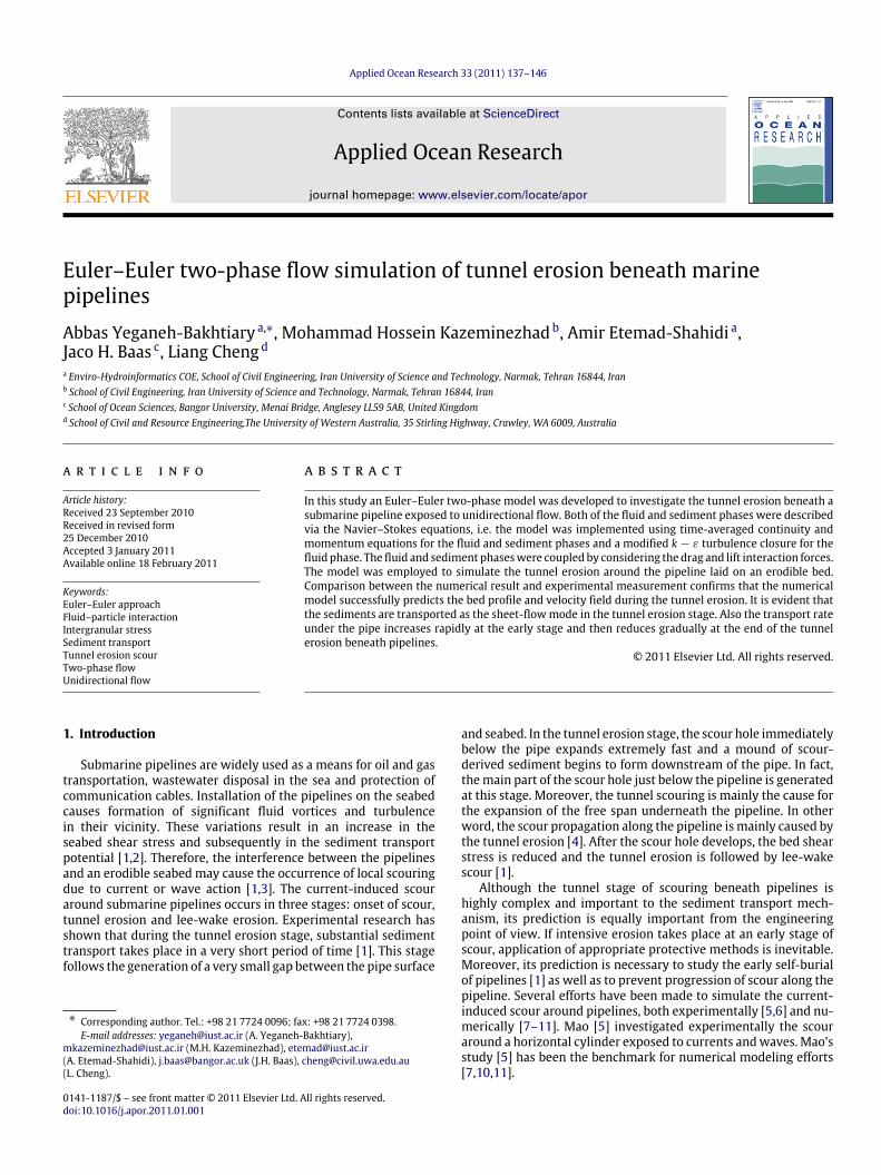
Fig. 1. Schematic domain and boundary condition for simulation of tunnel erosion.
The fluid phase mass conservation equation was used to calculatethe pressure field. The fluid concentration field was calculated us-ing the geometric conservation equation cf = 1 − cs.
The fluid phase equations consisted of two equations ofmomentum, a mass conservation and two turbulence closureequations were solved to approximate the mean velocity andturbulence field in the fluid phase. A pressure correction equationwas derived from themass conservation equation to determine thevelocity and pressure of the fluid. The aforementioned equationswere solved using the SIMPLE algorithm [26]. Once the fluidvelocity, pressure and turbulence characteristics were obtained,the sediment phase equations, consisting of two momentum andthe sediment phase mass conservation equations, were solved toobtain the sediment concentration and velocity fields.
3.2. Computational domain and boundary conditions
To simulate the tunnel erosion, a rectangular computationaldomain was considered (Fig. 1). The inlet and outlet boundarieswere located 10D (D is the pipe diameter) upstream and 20Ddownstream of the pipe center, respectively. A packed sand layerwith a thicknessDwas considered at the bottomof the domain. Thevolumetric sediment concentration within the sediment layer wasset to themaximum sediment concentration (cm). The depth of thesediment-free fluid zone above the packed sand layer was 4D. Atthe inlet boundary, a rough wall logarithmic velocity profile wasapplied [7] based on the friction velocity (u∗) and bed roughness(ks = 2.5d50).
At the free surface, the symmetry boundary conditions wereapplied.
∂u∂z
=∂us
∂z=
∂v
∂z=
∂vs
∂z=
∂k∂z
=∂ε
∂z= p = 0 (18)
csvs −υtf
σc
∂cs∂z
= 0. (19)
Zero normal gradients of all parameters except pressure wereapplied at the outlet boundary. At the first nodes located outsideof the cylinder, the hydraulically smoothwall boundary conditionshave been applied similar to that applied by Liang and Cheng [20].The sediment phase variables were also set to zero on the pipesurface.
The rough wall boundary condition was applied on the secondgrid placed below the packed sand layer surface. Applyingthis method led to simulation of pick-up phenomenon withoutobtaining unrealistic velocity components inside the packed sandlayer. Amoudry and Liu [18] used a similar method for defining thewall boundary condition. During development of the scour hole,the position of the packed sand layer surface was continuouslychanged and the location of the roughwallwas altered accordingly.The sediment phase velocity components were set to zero at therough wall boundary. The boundary conditions for k and ε at thebottom were based on the local equilibrium of turbulence energynear the bottom, taking account of the influence of the presence ofthe sediment grains [16,27].
a
b
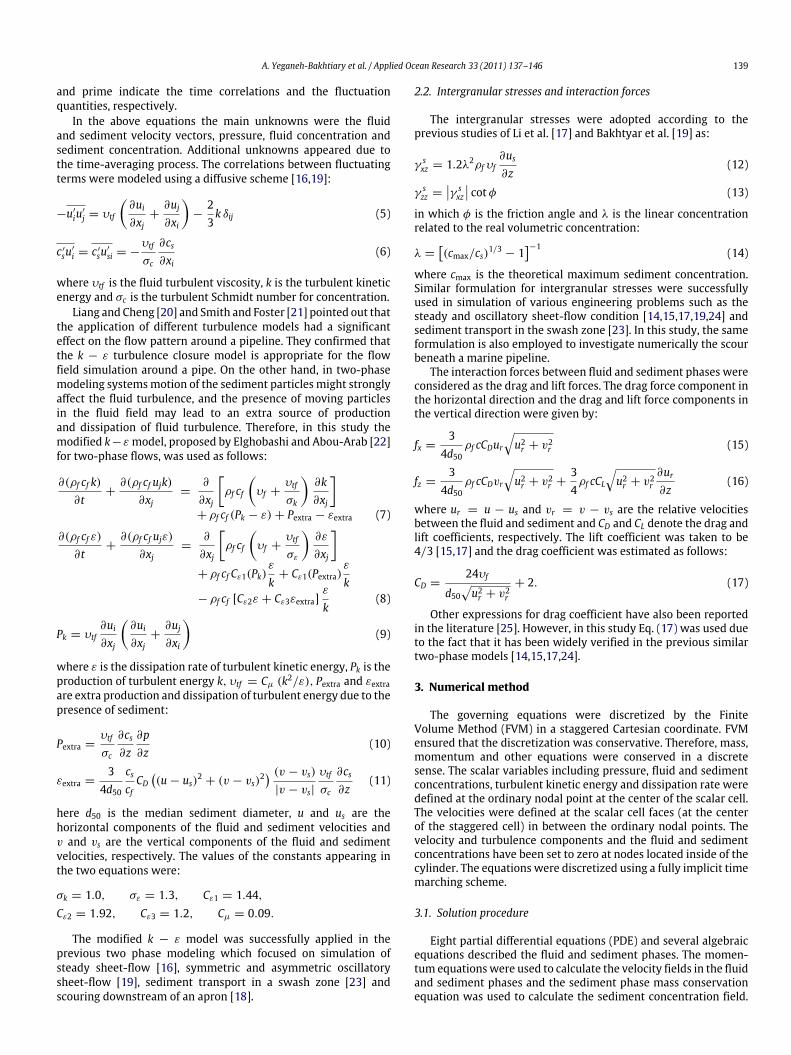
Fig. 2. Horizontal sediment velocity profile (a) in the total water depth (b) inthe near bed region. Solid lines—simulation; dots—near bed measurements withboroscope [29]; and triangles—measurements with ADV [29].
4. Model validation
Prior to applying the numericalmodel developed for simulationof tunnel erosion, it should be validated in simple case studies.As mentioned before, the two-phase model developed consistsof two parts; namely the fluid phase model and the sedimentphase model. The fluid phase model was extensively validated byKazeminezhad et al. [28] in the simulation of mean horizontalvelocity profiles around pipelines, vortex shedding and forcesacting upon marine pipelines. Here, the two-phase model wasvalidated against simulation of sheet-flow motion above a planebed considering the experimental condition of Dudely [29]. In thisexperimental work, the sediment velocity in a uniform, steadysheet-flow was measured with a boroscope near the bed and withanADV at a further distance. Themedian sediment diameter, waterdepth and Shields parameter were 0.25 mm, 15 cm and 1.02 cm,respectively.
To simulate the aforementioned experimental conditions, acomputational domain with 18 cm height was used, in which thebottom 3 cm is filled with sand and the upper 15 cm was purefluid zone at initial stage. Fig. 2(a) presents a comparison betweenthe simulated and measured horizontal sediment velocity. In thisfigure, the sediment velocity and elevationwere normalized by thefree stream velocity and sand diameter, respectively. Generally,
A. Yeganeh-Bakhtiary et al. / Applied Ocean Research 33 (2011) 137–146 141
Fig. 3. Vertical distribution of sediment concentration for the steady sheet-flowcondition identical to the experimental conditions of Dudley [29].
the agreement between the simulated and measured values isreasonably good. Themain discrepancy between themeasured andsimulated velocities occurred in the range of 15 < z/d50 < 50. Tofurther investigate the sediment velocity profile, themeasured andsimulated velocity profile in the near bed region was presented inFig. 2(b). From Fig. 2(a) and (b), it is clearly seen that the velocityfollows a linear profile close to the bed, while it follows a roughboundary log-law for z/d50 > 25.
Fig. 3 illustrates the vertical distribution of sediment concen-tration above the bed. As can be seen, the sediment concentrationis very high and approximately constant for z/d50 < 3. Abovethis layer, a sudden decrease occurs in the sediment concentration,which leads to the large gradient in the sediment concentration for3 < z/d50 < 15. The calculated sediment concentration is in goodaccordance with the steady sheet-flow concentration profile [30].The above numerical test shows that the present two-phase flowmodel works well in the simulation of sediment transport in thesheet-flow condition.
5. Simulation of tunnel erosion
The numerical test was identical to the clear-water experimentof Mao [5], which was used as a benchmark case for the modelingefforts. In the clear-water case, the scour and deposition causedonly by the local fluid tractive forces, without sediment transportfar from the pipe occurs. The pipe diameter, D, was 0.1 m andthe pipe was initially placed just above the sand layer without
any gap. The sand layer of thickness 1D consisted of sand withd50 = 0.36 mm; the water depth and the mean flow velocity were0.35m and 0.35m/s, respectively. The experimental conditionwasmodeled by assuming a logarithmic inlet velocity profile with afree surface velocity (u0) of 0.37 m/s. The velocity components ofthe sediment phase were set to zero at the inlet boundary. A finermesh was employed near the pipe and sediment bed layer. Themesh size was gradually increased to reach its maximum valuesnear the downstream, upstream and free surface boundaries. Thetime step and mesh resolutions were determined by iteration toensure the convergence of the results.
At the beginning of the simulation, a very small gap equal to onecell height (0.7 mm) between the packed sand layer and the baseof the pipewas imposed. Hence, the fluid flowed through the smallgap, and tunnel erosion was initiated. Since the fluid and sedimentphase equations were solved over the whole domain, there was noneed for re-meshing the domain for every time step. Fig. 4 showsthe mesh close to the pipe for both of the initial and disturbed bedprofiles. In contrast with other studies, the bed shape was flat atthe beginning of the simulation.
5.1. Scour development
In the aforementioned experiment, the equilibrium state wasreached after 370 min, with a maximum scour depth of 5.7 cm.After 10min, themaximum scour depthwas 2.7 cm. Hence, in 2.7%of the total scouring duration the scour depth reached 47% of itsequilibrium value. It is evident that the erosion rate was very highdue to tunnel erosion at this early scouring stage. Hereafter, thefirst 10 min of the experiment is called ts.
The first 10 min of tunnel erosion was simulated in moredetail. To validate the two-phasemodel in the simulation of tunnelerosion, the measured and simulated bed profiles at t = tsare compared in Fig. 5. The flow-sediment interface (bed profile)was selected as the location for which the volumetric sedimentconcentration equals 0.5 [11]. Fig. 5 also illustrates the numericalresults of Zhao and Fernando [11] for a similar case study. As canbe seen, the simulated bed profile from the previous and presentmodels demonstrates good agreement with the measurement.However, the present model provided a better estimation at theupstream side of the scour pit. This is partly due to applicationof a wall boundary condition below the sand layer surface,which avoided generating large velocities under the bed surface.In this study an initial flat bed profile was defined under thepipe, while a sinusoidal profile perturbation was assumed in theprevious studies. This assumption can cause some inaccuraciesin the simulation of the flow pattern and subsequently the bedprofile, especially at the tunnel erosion stage. Although the modelpredicted the bed profile well on the upstream side of the scour
1a b
Fig. 4. Mesh employed close to the pipe for (a) initial bed (b) disturbed bed.
142 A. Yeganeh-Bakhtiary et al. / Applied Ocean Research 33 (2011) 137–146
-2 -1 0
-1
0
1 2 3
Fig. 5. Comparison between measured and simulated bed profiles at t = ts .Dots—measurement [5]; solid line—present model; and dashed line—Zhao andFernando [11] simulations.
hole, some discrepancies still existed on the downstream sideof the pipe. This is due to the fact that the flow pattern ondownstream side of the pipe is rather complicated and changescontinuously due to the generation and movement of the mound.
The volumetric sediment concentration fields are depicted inFig. 6 to illustrate how the bed profile changes for different timesteps of tunnel erosion. At t = ts/16, a very small mound wasformed immediately downstream of the pipe. In time, the moundbecomes larger andmoves downstream as the scour hole develops.Comparison of the sediment concentration at different points intime shows that the upstream part of the scour hole was generatedfast in the initial stage of tunnel erosion. Fig. 6 clearly shows that,during the simulated period, substantial amounts of sand grainsmoved out from underneath the pipe and settled just downstreamof the pipe. This was mainly caused by a jet flow induced in the
scouring gap, prevailing during the tunnel erosion stage. Generallyfollowing the creation of a small gap between pipe and seabed, ajet-like flow prevails in the gap [5,31].
5.2. Flow pattern around pipeline
Flow streamlines at different time steps are presented in Fig. 7for different time instants. In the early stage of the simulation(t = ts/20), when the gap between the pipe and sand layer wasextremely small, a small-scale eddy formed upstream of the pipe(Fig. 7(a)). This was in line with the experimental observations[32–34]. This small-scale eddy was generated due to the existenceof a weak adverse pressure gradient in front of the pipe over thebed for small gap ratios. It partly deflected approaching flow awayfrom the gap and thus reduced the flow passing through the gap inthe initial stages of the tunnel erosion. At this stage, the maximumvelocity of the gap flowwas equal to 0.35u0. A large-scale eddywasalso formed behind the pipe in the initial stage of scour. The gapflow was not strong enough to noticeably affect the downstreameddy and it was deflected upwards behind the pipe. Therefore, thegap flow velocity reduced just downstream of the pipe, leadingto the deposition of the sediment and generation of the moundin the early stage of the scour. The upstream and downstreameddies rotate in a clockwise direction and, respectively, cause sandparticles to move away from and towards the pipe. In the casestudied the upstream eddy did not produce noticeable sedimenttransport and it just formed an obstruction to the approaching flownear the bed. The area occupied by the downstreamvortexwas alsolimited by the gap flow.
a b
c d
e
Fig. 6. Volumetric sediment concentration during the tunnel erosion.
A. Yeganeh-Bakhtiary et al. / Applied Ocean Research 33 (2011) 137–146 143
a
b
c
Fig. 7. Streamlines around pipe and eroded bed at: (a) t = ts/20, (b) t = ts/16 and(c) t = ts .
Fig. 7(b) presents the flow streamlines at ts/16. Comparisonbetween Fig. 7(a) and (b) shows that the upstream eddy sizedecreased as the gap ratio increased. Therefore, the gap flowgradually became stronger and its maximum velocity reached0.43u0. Although the gap flow was still not strong at this stage,it weakly affects the large-scale eddy by moving it towardsdownstream, especially in the near bed regions. At this instantanother small-scale eddy generates close to the pipe on thedownstream side. After a while, the increase of the scour depthcauses the small-scale eddy at the upstream of the pipe todisappear. Therefore, the jet velocity underneath the pipe becomesgreater. As the jet velocity and thus the mound height increases,a vortex was generated behind the mound. This is clearly seen inFig. 7(c), which displays the flow streamline at t = ts. Since thevortex rotates in a clockwise direction, this may lead to sedimenttransport toward the upstream face of the mound, which is inaccordance with Mao’s [5] observations. Moreover, two eddieswere seen just behind the pipe. The interaction between theseeddies was not large enough to create vortex shedding.
Fig. 8 shows the horizontal velocity profile at different locationsfor t = ts. At this stage, the maximum velocity of the jetunderneath the pipe was equal to 0.94u0. As can be seen,flow reversal behind the mound, e.g. at x/D = 1.5, 2, wasnot strong enough to noticeably transport the sand particlesin an upstream direction. Due to the lack of velocity profilemeasurements, quantitative comparisons were not possible.However, the agreement between the calculated velocity profilesand the observed flow patterns in the experimental case studies ofJensen et al. [35] was very good qualitatively.
One of the important novelties of this study is the simulationof tunnel erosion beneath the pipeline in more detail by assuming
Fig. 8. Horizontal fluid velocity profile around the pipe at t = ts .
Fig. 9. Streamlines around the pipe at early stage of scour for a sinusoidal initialbed.
an initial flat bed profile under the pipe. The results obtained inthe early stages of the simulation (Fig. 6) showed that the earlybed profiles did not exactly match with the assumed sinusoidalbed shape (Fig. 9) in the previous studies. However the maximumscour depth at t = ts/8 was almost equal to the amplitude ofthe assumed disturbance in the previous studies, the bed profile atthis stage was not symmetric similar to the sinusoidal bed profile.Simulations were carried out by assuming a sinusoidal bed profilebeneath the pipe to investigate its effects on the predictions. Fig. 9shows the streamline in the early stage of the simulation. Thesmall-scale eddy on the upstream side of the pipe was not formed,and the maximum gap velocity was equal to 0.50u0. Therefore, itwas expected that the model overpredicts the erosion rate in thescour pit. Fig. 10 shows the simulated bed profiles at t = ts for flatand sinusoidal initial bed profiles. It is seen that the applicationof a sinusoidal initial bed may lead to the further erosion at theupstream of scour hole; this overprediction was also observed inthe previous studies.
5.3. Hydrodynamics of sediment transport in tunnel scour
One of the advantages of the two-phase model is its capabilityto calculate sediment transport without employing an empiricalsediment transport rate equation. However, the model developedstill uses an empirical equation for calculation of intergranularstresses. Fig. 11 displays the sediment concentration profiles(solid line) just beneath the pipe (x/D = 0) at different timepoints. At all times, the sediment concentration profiles had aconvex upward shape near the stationary bed. The convex shapechanges to a concave upward shape further away from the bed.Fig. 11 also shows the sediment flux (qx) profile at x/D = 0.
144 A. Yeganeh-Bakhtiary et al. / Applied Ocean Research 33 (2011) 137–146
Fig. 10. Comparison between measured and simulated bed profiles at t = ts fordifferent initial bed profiles. Dots—measurement [5], solid line—simulation resultfor a flat initial bed, and dash–dot line—simulation result for a sinusoidal initial bed.
The sediment flux was computed by multiplying the horizontalsediment velocity by sediment concentration. From Fig. 11 it canbe concluded that during the tunnel erosion stage the maximumvalue of the sediment flux increases as the scour depth below thepipe increases.
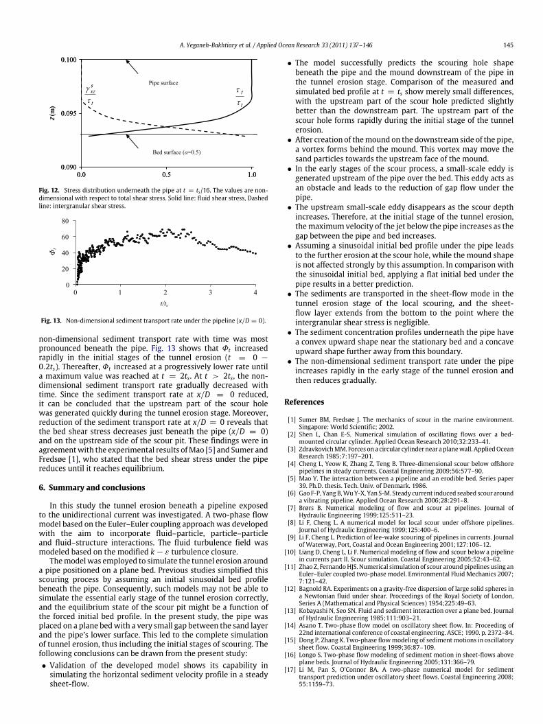
For further analysis of the hydrodynamics of scouring in thetunnel erosion in terms of fluid–particle and particle–particleinteractions, the non-dimensional fluid shear stress as well as theintergranular stress underneath the pipe at t = ts/16 are depictedin Fig. 12. The figure illustrates the shear stress distribution inthe early stage of the tunnel erosion scouring, during which anintensive sediment transport took place underneath the pipe andconsequently a severe particle–particle interaction due to veryfrequent interparticle collisions was the predominant mechanism.The total shear stress (τt ) near the bottom was expressed as thesum of the fluid shear stress (τf ) and intergranular shear stress(γ s
xz). The inertia regime, defined by Bagnold [12], was dominantnear the bed, while the macro-viscous regime was dominant atsome points under the pipe. In other words the intergranular
stress is much greater than the fluid shear stress close to thebed during the tunnel scour. Therefore, the interparticle forcesplay a significant role in the transmission of stress through theparticle–particle interaction. On the other hand, the reduction ofthe fluid shear stresses near the bottom indicates the decrease offluid turbulence energy level close to the bed, where the sedimentconcentration is very high.
According to the numerical results, the Shields parameter wasfound to be about 0.62 in the early stages of scouring beneathpipeline. Therefore, it may be interpreted that bed sedimentin the tunnel erosion stage was transported in the sheet-flowmode, which extended from the bottom to the point where theintergranular shear stress is negligible. As Yehaneh-Bakhtiaryet al. [36] pointed out ‘‘in a sheet-flow layer the high concentrationof moving grains induces a frequent interparticle collision; hencethe particle momentum in this layer is preserved and the velocitygradient is large. With a smooth shift to zero velocity at thebottom of high-density moving layer, the velocity profile shows anupward convex shape’’. Also, as indicated by Longo [16], the fluidturbulence almost vanishes in this concentrated layer due to thesignificant damping from predominant interparticle collisions ofmoving sand grains.
5.4. Sediment transport rate
To further investigate this observation, the non-dimensionalsediment transport rate, Φt below the pipe was calculated asfollows:
Φt =
zpzb
uscsdzg(s − 1)d3
(20)
here zb is the bed level elevation and zp is the elevation of thebase of the pipe above the initial bed. The time variation of the
a b
cd
e
Fig. 11. Volumetric sediment concentration (solid line) and sediment flux (dashed line) underneath the pipe at x/D = 0 for: (a) t = ts/16, (b) t = ts/8, (c) t = ts/4,(d) t = ts/2 and (e) t = ts .
A. Yeganeh-Bakhtiary et al. / Applied Ocean Research 33 (2011) 137–146 145
Fig. 12. Stress distribution underneath the pipe at t = ts/16. The values are non-dimensional with respect to total shear stress. Solid line: fluid shear stress, Dashedline: intergranular shear stress.
Fig. 13. Non-dimensional sediment transport rate under the pipeline (x/D = 0).
non-dimensional sediment transport rate with time was mostpronounced beneath the pipe. Fig. 13 shows that Φt increasedrapidly in the initial stages of the tunnel erosion (t = 0 −
0.2ts). Thereafter, Φt increased at a progressively lower rate untila maximum value was reached at t = 2ts. At t > 2ts, the non-dimensional sediment transport rate gradually decreased withtime. Since the sediment transport rate at x/D = 0 reduced,it can be concluded that the upstream part of the scour holewas generated quickly during the tunnel erosion stage. Moreover,reduction of the sediment transport rate at x/D = 0 reveals thatthe bed shear stress decreases just beneath the pipe (x/D = 0)and on the upstream side of the scour pit. These findings were inagreementwith the experimental results ofMao [5] and Sumer andFredsøe [1], who stated that the bed shear stress under the pipereduces until it reaches equilibrium.
6. Summary and conclusions
In this study the tunnel erosion beneath a pipeline exposedto the unidirectional current was investigated. A two-phase flowmodel based on the Euler–Euler coupling approach was developedwith the aim to incorporate fluid–particle, particle–particleand fluid–structure interactions. The fluid turbulence field wasmodeled based on the modified k − ε turbulence closure.
Themodelwas employed to simulate the tunnel erosion arounda pipe positioned on a plane bed. Previous studies simplified thisscouring process by assuming an initial sinusoidal bed profilebeneath the pipe. Consequently, such models may not be able tosimulate the essential early stage of the tunnel erosion correctly,and the equilibrium state of the scour pit might be a function ofthe forced initial bed profile. In the present study, the pipe wasplaced on a plane bedwith a very small gap between the sand layerand the pipe’s lower surface. This led to the complete simulationof tunnel erosion, thus including the initial stages of scouring. Thefollowing conclusions can be drawn from the present study:• Validation of the developed model shows its capability in
simulating the horizontal sediment velocity profile in a steadysheet-flow.
• The model successfully predicts the scouring hole shapebeneath the pipe and the mound downstream of the pipe inthe tunnel erosion stage. Comparison of the measured andsimulated bed profile at t = ts show merely small differences,with the upstream part of the scour hole predicted slightlybetter than the downstream part. The upstream part of thescour hole forms rapidly during the initial stage of the tunnelerosion.
• After creation of themound on the downstream side of the pipe,a vortex forms behind the mound. This vortex may move thesand particles towards the upstream face of the mound.
• In the early stages of the scour process, a small-scale eddy isgenerated upstream of the pipe over the bed. This eddy acts asan obstacle and leads to the reduction of gap flow under thepipe.
• The upstream small-scale eddy disappears as the scour depthincreases. Therefore, at the initial stage of the tunnel erosion,themaximum velocity of the jet below the pipe increases as thegap between the pipe and bed increases.
• Assuming a sinusoidal initial bed profile under the pipe leadsto the further erosion at the scour hole, while the mound shapeis not affected strongly by this assumption. In comparison withthe sinusoidal initial bed, applying a flat initial bed under thepipe results in a better prediction.
• The sediments are transported in the sheet-flow mode in thetunnel erosion stage of the local scouring, and the sheet-flow layer extends from the bottom to the point where theintergranular shear stress is negligible.
• The sediment concentration profiles underneath the pipe havea convex upward shape near the stationary bed and a concaveupward shape further away from this boundary.
• The non-dimensional sediment transport rate under the pipeincreases rapidly in the early stage of the tunnel erosion andthen reduces gradually.
References
[1] Sumer BM, Fredsøe J. The mechanics of scour in the marine environment.Singapore: World Scientific; 2002.
[2] Shen L, Chan E-S. Numerical simulation of oscillating flows over a bed-mounted circular cylinder. Applied Ocean Research 2010;32:233–41.
[3] ZdravkovichMM. Forces on a circular cylinder near a planewall. AppliedOceanResearch 1985;7:197–201.
[4] Cheng L, Yeow K, Zhang Z, Teng B. Three-dimensional scour below offshorepipelines in steady currents. Coastal Engineering 2009;56:577–90.
[5] Mao Y. The interaction between a pipeline and an erodible bed. Series paper39. Ph.D. thesis. Tech. Univ. of Denmark. 1986.
[6] Gao F-P, YangB,WuY-X, Yan S-M. Steady current induced seabed scour arounda vibrating pipeline. Applied Ocean Research 2006;28:291–8.
[7] Brørs B. Numerical modeling of flow and scour at pipelines. Journal ofHydraulic Engineering 1999;125:511–23.
[8] Li F, Cheng L. A numerical model for local scour under offshore pipelines.Journal of Hydraulic Engineering 1999;125:400–6.
[9] Li F, Cheng L. Prediction of lee-wake scouring of pipelines in currents. Journalof Waterway, Port, Coastal and Ocean Engineering 2001;127:106–12.
[10] Liang D, Cheng L, Li F. Numerical modeling of flow and scour below a pipelinein currents part II. Scour simulation. Coastal Engineering 2005;52:43–62.
[11] Zhao Z, FernandoHJS. Numerical simulation of scour around pipelines using anEuler–Euler coupled two-phase model. Environmental Fluid Mechanics 2007;7:121–42.
[12] Bagnold RA. Experiments on a gravity-free dispersion of large solid spheres ina Newtonian fluid under shear. Proceedings of the Royal Society of London,Series A (Mathematical and Physical Sciences) 1954;225:49–63.
[13] Kobayashi N, Seo SN. Fluid and sediment interaction over a plane bed. Journalof Hydraulic Engineering 1985;111:903–21.
[14] Asano T. Two-phase flow model on oscillatory sheet flow. In: Proceeding of22nd international conference of coastal engineering. ASCE; 1990. p. 2372–84.
[15] Dong P, Zhang K. Two-phase flowmodeling of sedimentmotions in oscillatorysheet flow. Coastal Engineering 1999;36:87–109.
[16] Longo S. Two-phase flow modeling of sediment motion in sheet-flows aboveplane beds. Journal of Hydraulic Engineering 2005;131:366–79.
[17] Li M, Pan S, O’Connor BA. A two-phase numerical model for sedimenttransport prediction under oscillatory sheet flows. Coastal Engineering 2008;55:1159–73.
146 A. Yeganeh-Bakhtiary et al. / Applied Ocean Research 33 (2011) 137–146
[18] Amoudry LO, Liu PL-F. Two-dimensional, two phase granular sedimenttransport model with applications to scouring downstream of an apron.Coastal Engineering 2009;56:693–702.
[19] Bakhtyar R, Yeganeh-Bakhtiary A, Barry DA, Ghaheri A. Two-phase hydro-dynamic and sediment transport modeling of wave-generated sheet flow.Advances in Water Resources 2009;32:1267–83.
[20] Liang D, Cheng L. Numerical modeling of flow and scour below a pipeline incurrents part I. Scour simulation. Coastal Engineering 2005;52:25–42.
[21] Smith HD, Foster DL. Modeling of flow around a cylinder over a scouredbed. Journal of Waterway, Port, Coastal and Ocean Engineering 2005;131:14–24.
[22] Elghobashi SE, Abou-Arab TW. A two-equation turbulence model for twophase flows. Physics of Fluids 1983;26:931–8.
[23] Bakhtyar R, Barry DA, Yeganeh-Bakhtiary A, Li L, Parlange J-Y, Sander GC.Numerical simulation of two-phase flow for sediment transport in the inner-surf and swash zones. Advances in Water Resources 2010;33:277–90.
[24] Liu H, Sato S. A two-phase flow model for asymmetric sheet flow conditions.Coastal Engineering 2006;53:825–43.
[25] Richardson JF, Zaki WN. Sedimentation and fluidization. Transactions of theInstitution of Chemical Engineers 1954;32:35–53.
[26] Patankar SV, Spalding DB. A calculation procedure for heat, mass andmomentum transfer in three-dimensional parabolic flows. InternationalJournal of Heat and Mass Transfer 1972;15:1787.
[27] Brørs B. Turbidity currentmodeling. Ph.D. thesis. The University of Trondheim.1991.
[28] Kazeminezhad MH, Yeganeh-Bakhtiary A, Etemad-Shahidi A. Numericalinvestigation of boundary layer effects on vortex shedding frequencyand forces acting upon marine pipeline. Applied Ocean Research 2010;32:460–70.
[29] Dudley RD. A boroscopic quantitative technique for sheet flowmeasurements.Master’s thesis. Cornell Univ. Ithaca. NY. 2007.
[30] Sumer BM, Kozakiewicz A, Fredsøe J, Deigaard R. Velocity and concentrationprofiles in sheet-flow layer of movable bed. Journal of Hydraulic Engineering1996;122(10):549–58.
[31] Mouazé D, Bélorgey M. Flow visualisation around a horizontal cylinder near aplane wall and subject to waves. Applied Ocean Research 2003;25:195–211.
[32] Bearman PW, Zdravkovich MM. Flow around a circular cylinder near a planeboundary. Journal of Fluid Mechanics 1978;89:33–47.
[33] Price SJ, Summer D, Smith JG, Leong K, Paidoussis MP. Flow visualizationaround a circular cylinder near to a planewall. Journal of Fluids and Structures2002;16:175–91.
[34] Lin WJ, Lin C, Hsieh SC, Dey S. Flow characteristics around a circular cylinderplaced horizontally above a plane boundary. Journal of EngineeringMechanics2009;135:697–716.
[35] Jensen BL, Sumer BM, Jensen HR, Fredsøe J. Flow around and forces on apipeline near a scoured bed in steady current. Journal of Offshore Mechanicsand Arctic Engineering 1990;112:206–13.
[36] Yeganeh-Bakhtiary A, Shabani M, Gotoh H, Wang SM. A three-dimensionaldistinct element model for bed-load transport. Journal of Hydraulic Research2009;47:203–12.