Euro area money demand - Empirical investigation using a ... · Prof. Dr. Christoph M. Schmidt RWI,...

Is Euro Area Money Demand

(Still) Stable?

Cointegrated VAR versus

Single Equation Techniques

#171

RUHR

Ansgar BelkeRobert Czudaj

ECONOMIC PAPERS

Imprint

Ruhr Economic Papers

Published by

Ruhr-Universität Bochum (RUB), Department of EconomicsUniversitätsstr. 150, 44801 Bochum, Germany

Technische Universität Dortmund, Department of Economic and Social SciencesVogelpothsweg 87, 44227 Dortmund, Germany

Universität Duisburg-Essen, Department of EconomicsUniversitätsstr. 12, 45117 Essen, Germany

Rheinisch-Westfälisches Institut für Wirtschaftsforschung (RWI)Hohenzollernstr. 1-3, 45128 Essen, Germany

Editors

Prof. Dr. Thomas K. BauerRUB, Department of Economics, Empirical EconomicsPhone: +49 (0) 234/3 22 83 41, e-mail: [email protected]

Prof. Dr. Wolfgang LeiningerTechnische Universität Dortmund, Department of Economic and Social SciencesEconomics – MicroeconomicsPhone: +49 (0) 231/7 55-3297, email: [email protected]

Prof. Dr. Volker ClausenUniversity of Duisburg-Essen, Department of EconomicsInternational EconomicsPhone: +49 (0) 201/1 83-3655, e-mail: [email protected]

Prof. Dr. Christoph M. SchmidtRWI, Phone: +49 (0) 201/81 49-227, e-mail: [email protected]

Editorial Offi ce

Joachim SchmidtRWI, Phone: +49 (0) 201/81 49-292, e-mail: [email protected]

Ruhr Economic Papers #171

Responsible Editor: Volker Clausen

All rights reserved. Bochum, Dortmund, Duisburg, Essen, Germany, 2010

ISSN 1864-4872 (online) – ISBN 978-3-86788-191-3

The working papers published in the Series constitute work in progress circulated to stimulate discussion and critical comments. Views expressed represent exclusively the authors’ own opinions and do not necessarily refl ect those of the editors.


Ansgar Belke and Robert Czudaj

Is Euro Area Money Demand

(Still) Stable?

Cointegrated VAR versus

Single Equation Techniques


Bibliografi sche Informationen

der Deutschen Nationalbibliothek

Die Deutsche Bibliothek verzeichnet diese Publikation in der deutschen National bibliografi e; detaillierte bibliografi sche Daten sind im Internet über: http//dnb.ddb.de abrufbar.

ISSN 1864-4872 (online)ISBN 978-3-86788-191-3

Ansgar Belke and Robert Czudaj1

Is Euro Area Money Demand (Still) Stable?

– Cointegrated VAR versus Single Equation

Techniques

AbstractIn this paper we present an empirically stable euro area money demand model. Using a sample period until 2009:2 shows that the current fi nancial and economic crisis that started in 2007 does not appear to have any noticeable impact on the stability of the euro area money demand function. We also compare single equation methods like the ARDL approach, FM-OLS, CCR and DOLS with the commonly used cointegrated Johansen VAR framework and show that the former are under certain circumstances more appropriate than the latter. What is more, they deliver results that are more in line with the economic theory. Hence, FMOLS, CCR and DOLS are useful in estimating standard money demand as well, although they have only been rarely applied for this purpose in previous studies.

JEL Classifi cation: C12, C22, C32, E41, E43, E58

Keywords: ARDL model; cointegration; euro area; fi nancial crisis; money demand

March 2010

1 Ansgar Belke, IZA Bonn and University of Duisburg-Essen, Campus Essen, Department of Economics; Robert Czudaj, University of Duisburg-Essen, Campus Essen, Department of Sta-tistics and Econometrics. – All correspondence to Ansgar Belke, University of Duisburg-Essen, Campus Essen, Department of Economics, 45117 Essen, Germany, e-mail: [email protected].

4

1. Introduction

Estimating a reliable money demand function is essential for the European Cen-tral Bank (ECB) with respect to its target of price stability (ECB (2004a), p. 49).Money plays a crucial role within the ECB’s monetary policy strategy since thereference value of money growth is seen as a benchmark for evaluating monetary de-velopments in the euro area. Potential output growth has been estimated at around2 to 2.5 percent, price stability implies consumer price inflation of below 2 percent,and a negative trend in velocity results in an increase of monetary growth in a rangebetween 0.5 and 1 percent. Under these assumptions, the reference value for mone-tary growth has been set at 4.5 percent per year and has not been revised any moresince (ECB (2004b), p. 64 and Dreger and Wolters (2008), p. 2). This referencevalue corresponds to one of the two pillars in the ECB’s two-pillar framework andis oriented at the widespread but often discussed view that money is a long-run butin some cases also a medium-run indicator of future inflation.1,2 Hence, if, and onlyif, the demand for money turns out to be verifiable stable, changes in the stock ofmoney can be expected to have a predictable impact on inflation (Belke and Polleit(2009), pp. 677, 681, and Issing et al. (2001), p. 6). However, different inflationforecast approaches such as the p-star model require a reliable estimation of a moneydemand function.3 Therefore the stability issue has received particular attention inthe literature since M3 growth started to accelerate in 2001 due to the terroristattacks of September 2001 and the burst of the new economy bubble. Instabilityemerged at that time since large funds were reallocated into safe and liquid assetsthat are part of M3 during that time (Belke and Polleit (2009), p. 136). Currently,in the global financial and economic crisis that started in 2007, the stability issuegains even more interest.Hence, the main purpose of our paper is to check empirically whether the moneydemand function in the euro area is (still) stable in its parameters. Moreover, wewould like to assess which estimation technique is the preferred one to deal with thisissue. Finally, it is of interest whether the financial crisis and the efforts spent bythe ECB to manage the former by means of lowering its policy rates and conductingunorthodox monetary policies has had any effect on the magnitude of the coefficientsand/or the stability of the long-run money demand function. We feel legitimized tostress again that the stability of the money demand equation is an important pre-requisite of a sound conduct of the monetary pillar of the ECB’s monetary policystrategy.

1"Inflation is always and everywhere a monetary phenomenon." (Milton Friedman, WincottMemorial Lecture, London, September 16th 1970)

2This is in line with ECB (2004b), p. 47 and Benati (2009).3See, for example, Nicoletti-Altimari (2001), p. 13.

5

In the following, we take the theoretical and empirical findings in the previous lit-erature as a starting point of our analysis and use commonly accepted econometricmethods. Taking into account exogeneity issues, focus on the search for a cointe-gration relation between money aggregates and related variables. Moreover, apply avariety of different econometric techniques to compare their estimation results andtheir usefulness in identifying and determining the euro area money demand func-tion. Accordingly, we apply the cointegrated VAR approach by Johansen (1995), theARDL approach by Pesaran, Shin and Smith (1999, 2001) and other single equationmethods such as fully-modified ordinary least squares (FM-OLS), canonical coin-tegration regression (CCR) and dynamic OLS (DOLS), which all will be discussedlater. A further aim of this paper is to check the impact of the sample size in findinga stable cointegrating relation.The remainder of the paper is organized as follows. In the next section we presentthe underlying theory, which draws the connection between money and the othervariables of interest. In section 3 we highlight the available recent studies on euroarea money demand in order to compare our settings and results with theirs. Themain part of our study, the econometric analysis, is presented in section 4, where wediscuss the data used and check the variables for stationarity and for cointegrationsequentially within the Johansen framework and the ARDL approach. Furthermore,we look into the constancy of our estimated parameters. We check our estimationresults for robustness in section 5. For this purpose, we apply the other three above-mentioned single equation methods and different lag lengths. Section 6 concludesand gives an outlook on further research.

2. Theory of money demand

In the corresponding theoretical and empirical literature, different specifications ofmoney demand functions are used.4 These studies have generally in common thata money demand equation contains a scale variable to describe the economy’s levelof transactions and a variable reflecting the opportunity costs of holding money.Whereas there is general agreement in the literature in the case of choosing a scalevariable, the selection of the opportunity cost variable repeatedly results in somecontroversy. Hence, the literature tends to use different interest rates, interest ratedifferentials or the inflation rate as a proxy for the opportunity costs. According toFase and Winder (1998), a common specification of the money demand function has

4See Lütkepohl and Wolters (1999a) for single- and multi-country studies, Golinelli and Pastorello(2002), pp. 374-375 and Nautz and Ruth (2005), p. 9.

6

the following form:5

(m− p)t = β0 + β1yt + β2ilt + β3i

st + β4πt + ut, (1)

where m denotes a monetary aggregate (M1, M2 or M3), p represents a measureof the prices level, y stands for a measure of real income as the scale variable, il

and is are the long-run and the short-run interest rate, respectively, π representsthe inflation rate and u the error term. The short-term interest rate is a proxyof the M3 "own rate" and the long-term interest rate characterizes the return onalternative assets (Coenen and Vega (2001), pp. 729-730). Except for both interestrates, we take all variables in logs. We expect the following signs of the coefficients:β1 > 0, β2 < 0, β3 > 0 and β4 < 0. The Baumol-Tobin model and the quantitytheory predict the income elasticity to be β1 = 0.5 and β1 = 1, respectively (Baumol(1952), Tobin (1956) and Friedman (1956)). However, in the empirical literatureone tends to find empirical realizations of income elasticities for a broad moneyaggregate which are slightly beyond unity. This pattern is often said to be dueto the neglect of the wealth effect (Coenen and Vega (2001), p. 728, and Booneand van den Noord (2008), p. 531). The estimated coefficients of both interestrates represent semi-elasticities given that both variables have not been taken aslogarithms as suggested by Fair (1987), p. 473.

3. Recent studies on euro area money demand - A

survey

This section examines several important critical specification issues and procedureswhen empirically modelling money demand in the euro area. In order to alludeto the more relevant choices, we define the long-run equation as proposed in thepreceding section. Table 1 shows the different specifications of the money demandequation in the euro area taken from earlier studies and their coefficient estimates.The estimated income elasticity turns out to take values between 1.1 to 1.5 in mostof the studies. This range is broadly in line with predictions from theory and theshort deviation from unity is often explained within the standard portfolio approachby the neglect of a wealth variable. Some authors try to cope with this issue byusing different proxies of wealth such as financial wealth or stock prices, respectively(Fase and Winder (1998), p. 509, Bruggeman et al. (2003), pp. 30-32, and Beyer(2009), pp. 11-22).

- Table 1 about here -

5Fase and Winder (1998), p. 512, use a wealth variable in addition to our specification.

7

3.1. Opportunity costs of holding money

In the empirical literature the operationalization of the opportunity costs of holdingmoney is often discussed rather controversially. Our choice of taking the short-term and long-term interest rates as proxy of the M3 "own rate" and the returnon alternative assets respectively goes back to Coenen and Vega (2001), pp. 729-730. Brand and Cassola (2004), p. 821, confine themselves to use only the long-run interest rate to seize the opportunity costs, since, from their perspective, thelong-term interest is able to sufficiently capture the dynamics of the interest ratedifferential between the long-run interest rate and the M3 "own rate" and thissimplification reduces the complexity of the model.Calza et al. (2001) apply two different specifications of the opportunity cost variablein their model. They insert the difference between the short-term interest and theM3 "own rate" as well as the difference between the long-term interest and the M3"own rate". Moreover, they show that this specification only has a slight impacton the estimation results. However, they do not include the inflation rate in theirmodel because they do not attach any additional explanatory content with respectto money demand to it - at least compared to the nominal long-term interest rate(Calza et al. (2001), p. 8). Nevertheless, inflation is usually interpreted, for instanceby Dreger and Wolters (2009), as a part of the opportunity costs, as it representsthe costs of holding money in spite of holding real assets (Ericsson (1999), p. 38,and Dreger and Wolters (2009), pp. 112-113). Bruggeman et al. (2003), p. 37,demonstrate how to construct the "own rate of return" of euro area M3, which isused in a variety of other recent studies as well.

3.2. The aggregation problem

A further problem often encountered when estimating the money demand functionfor the euro area is the availability of aggregated euro area data prior to 1995. Someauthors try to construct euro data by aggregating the national data of M3, GDP,consumer prices and interest rates. Scale variables are denominated in nationalcurrencies and should first be converted into euro by using the irrevocably fixedexchange rates6 and then summed up to the euro area aggregate time series, as itis done, for instance, by Bruggeman et al. (2003), pp. 10-11. An advantage of thismethod is that it is consistent with the method that is used by the ECB since thestart of Stage Three of EMU. Nevertheless, Fagan and Henry (1998), p. 495, presentan alternative aggregation method, the so-called index method. According to this

6The ECB has announced the irrevocably fixed exchange rates on December 31, 1998 (and deter-mined on June 19, 2000, in the case of Greece, on July 11, 2006 for Slovenia, on July 10, 2007for Malta and Cyprus and on July 7, 2008 for Slovakia).

8

method the log-level index for the euro area series is defined as the weighted sum ofthe log-levels of the national series, where the weights are the shares of the nationalGDP in euro area GDP in 2001 measured at PPP exchange rates. Applying thismethod avoids possible spurious correlation among the euro area series, which aremerely due to changes in the exchange rates. In contrast to the so-called exchangerate method the index method is also applicable to interest rates. In this context itis possible to use the M3 shares instead of the GDP shares of each country as weights(Bruggeman et al. (2003), p. 12). Fase and Winder (1998) discuss the effects basedon alternative aggregation methods. Winder (1997) and Beyer et al. (2001) providea general discussion on aggregation issues underlying the construction of historicaleuro area data. To apply any aggregation method, one requires a quite large sampleof national data of the 16 euro area countries.

3.3. Appropriate econometric techniques and the issue of

weak exogeneity

Most of the studies we refer to in the context of euro area money demand esti-mation apply the Johansen framework to identify cointegration relations amongthe variables and to estimate the coefficients of the cointegrating vectors and theerror-correction parameters, which indicate the speed of adjustment from short-rundeviations to the long-run equilibrium. Generally, the empirical literature we surveyin this paper (see Table 1) uses quarterly data. Thus, one should to estimate a VARmodel with four lags, but the consensus is the estimation with two lags to avoid anoverly strong decrease in degrees of freedom. To estimate a VAR model in the vectorerror-correction representation, one important step is to select a trend specification(Johansen (1995), pp. 80-84).The empirical literature usually applies an unrestricted constant, allowing for a lin-ear trend in the variables but not in the cointegrating relations.7 Although, Brandand Cassola (2004), p. 823, test the model with a restricted constant as well, allow-ing for no linear trend in the variables and the cointegrating equations. If the foundcointegration rank is larger than one, identifying restrictions have to be imposedand then to be tested. The literature delivers different versions of model restric-tions.8 After estimating the coefficients, the variables are usually tested for theirweak exogeneity vis-à-vis the system. Intuitively, weak exogeneity of right-hand sidevariables allows us to condition on these variables without specifying their generat-ing process with no loss of useful information (Engle et al. (1983) pp. 282-283, andUrbain (1992) pp. 188-189). Regarding this property, the available studies arrive at

7See, for example, Coenen and Vega (2001), p. 733.8See, for instance, Coenen and Vega (2001), pp. 728-729, 733-736 or Brand and Cassola (2004),pp. 818-819.

9

conflicting results, while, for instance, Brand and Cassola (2004), p. 824, come upwith the striking result that no variable included in their approach can be consideredto be weakly exogenous, Coenen and Vega (2001), p. 735, find weak exogeneity ofthe GDP variable, both interest rates and the inflation rate.According to Enders (2010) who refers to an example originally introduced by Jo-hansen and Juselius (1990) it might be possible to argue that GDP should be weaklyexogenous (Enders (2010), p. 407, and Johansen and Juselius (1990), pp. 181-206).However, some authors claim that the Johansen procedure could be in certain cir-cumstances susceptible to spurious cointegration (Gonzalo and Lee (1998), p. 149).Taking this potential flaw into account, several authors estimate the cointegratingequation by means of some alternative techniques such as the Engle and Granger(1987) procedure, the autoregressive distributed lag (ARDL) model proposed by Pe-saran and Shin (1999) and the fully-modified OLS approach by Phillips and Hansen(1990) as well. Applying this wide array of techniques might well serve to check forrobustness of the results. By doing so, we follow Calza et al. (2001), who show thattheir results originally produced within the Johansen framework are quite robust tothe use of alternative techniques (Calza et al. (2001), pp. 10, and 30).

3.4. Stability tests

In a variety of studies stability tests such as the recursive estimated coefficients orthe Chow test are used to check for stability of the estimated long-run parametersand to identify possible structural breaks (Chow (1960)). For instance, Brand andCassola (2004), Coenen and Vega (2001) and Calza et al. (2001) do not find anyevidence of a structural break in their sample periods ranging from 1980:1 to 1999:3,from 1980:4 to 1998:4 and from 1980:1 to 1999:4, respectively (Brand and Cassola(2004), pp. 826-828, Coenen and Vega (2001), pp. 738-739, and Calza et al. (2001),pp. 13, and 22-24). Calza and Sousa (2007) provide three reasons why M3 moneydemand has been more stable in the euro area than in other large economies. First,they argue that instability in the money demand in some economies is country-specific. Second, from their point of view financial innovation appears to have hada weaker impact on money demand in the euro area than, for instance, in the US.Third, they make a more technical point, i.e. the aggregation of the money demandof the individual euro area countries could be held responsible for the stability ofthe money demand in the euro area.Coenen and Vega (2001) and Funke (2001) use a dummy variable to model a struc-tural break in 1986, which should, corresponding their view, take into account spe-cial developments in German data according to which some debt securities weresubjected to reserve requirements (Coenen and Vega (2001), p. 733). Bruggeman

10

et al. (2003) criticize the above-mentioned stability tests, arguing that these testsonly make use of a part of the sample and apply alternative techniques to checkfor stability.9 However, they get no conflicting results compared to the commonlyused techniques for their sample from 1980:4 to 2001:4 (Bruggeman et al. (2003),pp. 19-25). Hall et al. (2008) re-estimated the Calza et al. (2001) model over theperiod 1980:1 to 2006:3 and found a structural break in 2001:2 (Hall et al. (2008),p. 13, and De Santis et al. (2008), pp. 9-10, and 41-42). Dreger and Wolters (2008),pp. 7, and 19, use a dummy variable referring to a structural break in 2002:1.Although many researchers face the stability issue, there is still a gap in analyzingthe impact of the financial crisis on euro area money demand, since the observationperiod of the majority of the studies ends before 2007. Exceptionally, Beyer (2009),pp. 22-24, 27-39, and 46-53, shows that euro area money demand is still stable atthe start of the crisis by applying the same methods as Bruggeman et al. (2003).

3.5. Further modifications

Besides the implementation of a wealth effect variable into the model further amend-ments are proposed in the literature. For example, Calza et al. (2001) extend theirbasic model with the world oil price index as a proxy of import prices in order tocorrect for potential difficulties arising from the application of the GDP deflator as ameasure of the general price level for relatively open economies (Calza et al. (2001),pp. 14, 34, and Lütkepohl and Wolters (1999b), p. 109). Greiber and Setzer (2007),pp. 8, and 13, augment their money demand specification by the real residentialproperty price index and the housing wealth indicator, respectively.Beyer (2009) as one of the most recent empirical studies on the euro area moneydemand function adds housing wealth to the model as well to account for the wealtheffect. What is more, Greiber and Lemke (2005) implement uncertainty as an addi-tional variable in their money demand model. Hamori and Hamori (2008) estimatethe money demand for M1, M2 and M3 based on a panel analysis, which includeseleven different countries. Finally, Carstensen et al. (2009) estimate euro area moneydemand for four countries (Germany, France, Spain and Italy) individually and ag-gregated (Beyer (2009), pp. 11-24, Greiber and Lemke (2005), pp. 6, 16, Hamoriand Hamori (2008), pp. 275-282, and Carstensen et al. (2009), pp. 77-82).

9They use the fluctuation test suggested by Hansen and Johansen (1999), examine the constancyof β using the Nyblom (1989) tests studied by Hansen and Johansen (1999) and the constancyof the Φ, Γ1, and α parameters using the fluctuation test developed by Ploberger et al. (1989).

11

4. Empirical analysis

We start our empirical analysis with the description of the underlying data. Further,we assess the order of integration of the variables and the lag length which appearsadequate to properly apply the Johansen framework. We use the latter to comeup with some basic estimation results. What is more, additional estimations whichapply the ARDL approach complete the whole picture and serve as a robustnesscheck of the estimation results gained with the Johansen procedure. Moreover, wecheck our parameter estimates for constancy. We do so applying two different andsuitable data sets which are described in the following.

4.1. The data

In our study we use quarterly data ranging from 1995:1 to 2009:2. The underlyingtime series are taken from the ECB Statistical Data Warehouse. As our measure ofthe money aggregate, we apply quarterly averages of the seasonally adjusted month-end stocks of M3. We take the seasonally adjusted real gross domestic product(GDP) as a proxy of the scale variable10 and rely on the the GDP deflator (1995 =100) as our measure of the price level. The inflation variable is constructed by theannualised quarterly changes in the GDP deflator. The three-month Euribor moneymarket rate (short-term interest rate) measures the return on assets included inthe definition of M3 and the 10-year treasury bond yield (long-term interest rate)characterizes the return on assets excluded from the monetary aggregate.One problem in estimating a reliable money demand function for the euro areais the still relatively small sample size, resulting of the fact that the EuropeanMonetary Union (EMU) is still a quite young institution. The only way to arriveat a larger sample is to aggregate the national data prior to 1995 on a euro arealevel. For instance, Coenen and Vega (2001) followed this way.11 Hence, we usetheir aggregated time series ranging from 1980:1 up to 1994:4 to extend our sampleand to check the impact of the sample size by estimating our model for the longertime horizon again.

4.2. Stationary tests

To test for the usual time series properties of the data we first conduct some unitroot tests. To check for cointegration between the variables within the Johansenframework we have to establish first that the variables of interest are integrated oforder one (I(1)). As usual, we apply the augmented Dickey-Fuller test (ADF test)10Personal consumption expenditure could be used for this purpose as well.11They publish their aggregated time series in their earlier working paper from 1999 Coenen and

Vega (1999), pp. 33-34.

12

and the Phillips-Perron test (PP test) to test the null of a unit root in the time seriesand refer to the critical values tabulated by MacKinnon (Dickey and Fuller (1979),Phillips and Perron (1988), MacKinnon (1991) pp. 271-274 and MacKinnon (1996)pp. 603-616). We present the resulting empirical realizations of the t-statistics andthe p-values for the levels and the first differences for both samples in Table 2.


The results for the small sample (1995:1-2009:2) indicate that, except for πt,all variables of interest seem to be non-stationary, i.e. I(1). However, the rateof inflation appears to be integrated of order zero (I(0)), probably because it isconstructed of the first difference of the GDP deflator. Hence, πt and the GDPdeflator pt are again tested for stationarity with the ADF and the PP test droppingthe intercept from the auxiliary test equation. The corresponding results conveysome evidence that the inflation rate πt is I(1) and that pt inevitably amounts toI(2) as it is often also the result in various other studies such as Johansen andJuselius (1990).12 However, our results are often highly dependent on the numberof lags used in the specifications of the test equation and also on the number ofobservations used. Furthermore, it is well-known that the univariate stationarytests have a rather low power. Hence, it appears useful in our context to checkthe stationarity properties with multivariate tests as well (DeJong et al. (1992) andCoenen and Vega (2001), p. 732). Hence, we assume all variables to be I(1) just inline with Wesche (1998), p. 21, and others. Correspondingly, we feel legitimized toargue that the Johansen framework is applicable in our context.The results for the larger sample (1980:1-2009:2), which are displayed in the bottompart of Table 2, tell us the same story, but turn out to be even more significantespecially for ilt, which indicates following Schwert (1989) that our first and basicsample period might be too short.

4.3. Empirical VAR model

Consider a vector autoregressive (VAR) model of order p following Sims (1980), pp.15-33:

Yt = A1Yt−1 + . . .+ ApYt−p + ΦXt + εt, (2)

where Yt is a k-dimensional vector of non-stationary I(1) variables, Xt is a d-dimensional vector of deterministic variables, and εt is a vector of innovations withzero mean and covariance matrix Ω. In the following, we estimate a VAR(p = 2)

12The results are available upon request.

13

model with Yt =[(m− p)t yt ist ilt πt

]′, k = 5 and d = 0 in order to test for

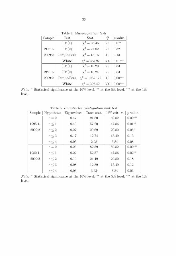
cointegration. We do not a priori include dummy variables and, thus, let the dy-namic structure absorb potential shocks, because a thorough visual inspection ofthe series does not reveal a permanent break in the cointegrating relation amongthe used variables.First of all, we check for the adequate lag length to be used for the VAR modeland test the usual properties of the residuals. Table 3 shows that the likelihoodratio (LR), the final prediction error (FPE) and Hannan-Quinn (HQ) informationcriterion all recommend, in case of the small sample, a lag length of p = 2, whileapplying an unrestricted VAR model up to a maximum lag length of 5. Only theAkaike (AIC) and the Schwarz (SC) criterion indicate a lag length of p �= 2.13 Ourresults of the lag length selection criteria for the large sample are not tabulatedhere. Nevertheless, their application leads to the same empirical pattern with evenmore unambiguity than in the smaller sample period.14 Later on in section 5.2 weadditionally apply different lag lengths to check the robustness of our results.Table 4 displays the results of our misspecification tests for both samples. The mod-ified White test by Kelejian (1982) lets us suspect the residuals to be heteroskedastic(White (1980)).According to the Jarque-Bera test with Cholesky orthogonalization as suggested byLütkepohl (2007), pp. 174-181, the assumption that the residuals are normally dis-tributed appears to be violated in case of the larger sample. However, the null ofserial correlation of order 1 and 2 is rejected in case of both samples.

- Tables 3 and 4 about here -

4.4. Cointegration analysis

Since we cannot reject that our macro time series contain a unit root, we feel le-gitimized to apply the ordinary VAR-based cointegration test which sticks to themethodology developed by Johansen.15 Let us consider our VAR(p) model adaptedto the VEC representation:

ΔYt = ΠYt−1 +

p−1∑j=1

ΓjΔYt−j + ΦXt + εt. (3)

Granger’s representation theorem asserts that if the coefficient matrix Π has reducedrank r < k, then there exist k × r matrices α and β each with rank r such that

13All the criteria are discussed by Lütkepohl (2007), pp. 146-157.14The results are available upon request.15See Johansen (1988), pp. 233-253, Johansen (1991), pp. 1552-1564, Johansen (1995) and Jo-

hansen and Juselius (1990), pp. 170-180, 193-206 for details.

14

Π = αβ′ and β′Yt is I(0) (Engle and Granger (1987), pp. 255-258). r is the numberof cointegrating relations (the cointegrating rank) which we identify using the tracestatistics. Moreover, each column of β is a cointegrating vector. The elements of αrepresent the adjustment parameters in the VECM. Γj capture the short-run effectsof the time series. Johansen’s method consists of estimating the matrix Π from anunrestricted VAR with a maximum likelihood technique and testing whether we canreject the restrictions implied by the reduced rank of Π.The upper part of Table 5 displays our results of the unrestricted cointegration ranktest for the short sample.16 The trace test rejects the hypothesis of no cointegrationrelation and the hypothesis of one cointegration relation between the variables andaccepts the hypothesis of a cointegration rank of a maximum of 2 at a 5% significancelevel. Accordingly, we feel legitimized to assume two cointegration relations (r = 2)among the variables and to estimate the cointegrating equations with the maximumlikelihood procedure, as suggested by Johansen.


However, before estimating Π one has to make an assumption about the determin-istic trend specification of the used time series. One can choose between five trendspecifications (Johansen (1995), pp. 80-84). As stated above, the two specificationsusually recommended in the empirical literature are the one including levels Yt with-out deterministic trends and cointegrating equations with restricted intercepts andthe other one containing levels Yt with linear deterministic trends and cointegratingequations with unrestricted intercepts.17 Following Coenen and Vega (2001), wechoose the second specification and estimate Π assuming linear trends in the leveldata and a unrestricted constant in the cointegrating equations.Estimating the parameters α and β within

ΔYt = αβ′Yt−1 +

p−1∑j=1

ΓjΔYt−j + ΦXt + εt, (4)

using Yt =[(m− p)t yt ist ilt πt

]′from the basic sample (1995:1-2009:2), two

lags, r = 2 and the trend specification mentioned yields two cointegrating equationsβ′Yt which have the below-stated form:

(m− p)t = −9.80 + 1.45∗∗∗yt − 12.32∗∗∗πt, (5)

16The test is applied using p-values taken from MacKinnon et al. (1999), pp. 570-576.17See, for example, Brand and Cassola (2004), p. 823 and Coenen and Vega (2001), p. 733,

respectively.

15

ilt = −0.06 + 1.61∗∗∗ist + 2.88∗∗∗πt. (6)

The first cointegration equation can be interpreted as the money demand functionand the second one as an equation combining the term structure of interest ratesand the Fisher inflation parity. Conditional on the choice of cointegration rank, theLR test does not reject the imposed restrictions at conventional levels based on theχ2-statistic of 3.82 with df = 2 and a p-value = 0.15. The coefficients have the pre-dicted signs and turn out to be highly significant. Especially, the estimated incomeelasticity nearly reveals the same magnitude as proposed by the standard literature(1.1 to 1.5). The estimated empirical realizations of the adjustment parameters tothe long-run equilibrium α take the following values:

α =

⎡⎢⎢⎢⎢⎢⎢⎣

−0.07∗∗∗ −0.25∗∗∗−0.02 0.07

0.01 0.10∗∗∗

−0.04∗∗∗ −0.07−0.12∗∗∗ −0.17

⎤⎥⎥⎥⎥⎥⎥⎦, (7)

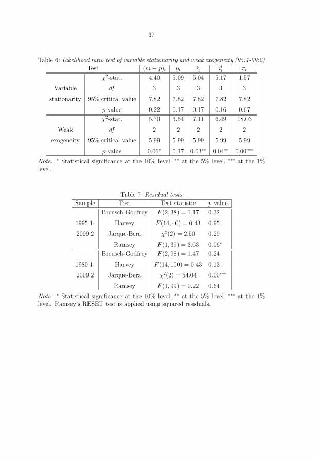
where the first element of the first column represents the error-correction parameterof the estimated money demand function. Accordingly, the speed of adjustment tothe long-run equilibrium seem to be very low.Additionally, the null of stationarity given the cointegration space is tested applyingthe likelihood-based procedure (LR test), which characterizes a multivariate versionof the Dickey-Fuller test, against the alternative of non-stationarity. What is more,the null of weak exogeneity of the variables is checked with the LR test as well. Theresults are stated in Table 6.


According to our results, all series seem to be stationary. However, on the onehand this results is highly dependent on the chosen cointegration rank r. On theother hand, our results could be interpreted in a way that the ARDL approach isin this case a more appropriate technique than the Johansen framework, because itdoes not require a priori knowledge that all variables are I(1) (Pesaran and Shin(1999), Belke and Polleit (2006a), Belke and Polleit (2006b) and Belke and Polleit(2006c)).According to Enders (2010), it would not at all be surprising if yt would be the onlyweakly exogenous variable in our variable set (Enders (2010), p. 407). Exactly thisresult is already indicated by the second element of the first column of α, whichtakes an empirical value around zero.We enacted the same procedure also for the larger sample period (1980:1 to 2009:2)

16

to make our findings more robust. Again, the results of the trace test let us acceptthe hypothesis of at most two cointegration ranks (see lower part of Table 5).Using the same restrictions as applied for the short sample our estimation of thecointegrating equations yields the following results:

(m− p)t = −3.68 + 1.01∗∗∗yt − 1.77∗∗∗πt, (8)

ilt = 0.01 + 0.82∗∗∗ist + 0.22∗∗∗πt. (9)

Whereas the estimated coefficients also have the same signs as in case of the smallersample period and are again highly significant, their magnitudes seem to be evenmore striking according to the theoretical predictions and the previous empiricalstudies. Conditional on the existence of three cointegrating relations, the LR testhardly accepts the imposed restriction at a 1% significance level based on the χ2-statistic of 9.41 with df = 2 and a p-value = 0.01.

α =

⎡⎢⎢⎢⎢⎢⎢⎣

0.15∗∗∗ 0.64∗∗∗

0.14∗∗∗ 0.98∗∗∗

0.00 0.04

−0.00 −0.08−0.74∗∗∗ −3.18∗∗∗

⎤⎥⎥⎥⎥⎥⎥⎦

(10)

The speed of adjustment to the long-run equilibrium given above seems to be abit larger and the error-correction term of the money demand has a positive signnow.

4.5. ARDL approach

One popular method to check how robust the estimated money demand equationis to apply additional estimation techniques. The autoregressive distributed lag(ARDL) model by Pesaran, Shin and Smith (1999, 2001) is usually applied in ourcontext as well (for example, Coenen and Vega (2001), pp. 736-741 and Calza et al.(2001), pp. 12-13, 30). The ARDL approach has the advantage that it does notrequire all variables to be I(1) as the Johansen framework and it is still applicableif we have I(0)- and I(1)-variables in our set. As stated above and closely following,

17

for instance, Belke (2010) and Narayan and Smyth (2004), it is potentially at leastas appropriate in such a case as the Johansen framework.18

The estimated error-correction representation of the ARDL model with unrestrictedintercept and without trend has the following general specification with p and qi

lags:

Δ(m− p)t = α0 +

p−1∑j=1

ψjΔ(m− p)t−j +

q1−1∑j=0

α1jΔyt−j +

q2−1∑j=0

α2jΔist−j (11)

+

q3−1∑j=0

α3jΔilt−j +

q4−1∑j=0

α4jΔπt−j + γ0(m− p)t−1 + γ1yt−1 + γ2ist−1 + γ3i

lt−1 + γ4πt−1 + ut,

where the γi denote the long-run parameters and ψj and αij the short-run dynamiccoefficients of the model. ut is uncorrelated with the lagged endogenous and exoge-nous regressors and the first differences of the exogenous regressors and their lags.First, we estimate an ARDL model with p = q1 = . . . = q4 = 2 lags according tothe SC as proposed by Pesaran and Shin (1999), p. 374, using the short sample(1995:1-2009:2) and second, we normalize coefficients by imposing βi =

γi

γ0. The

corresponding cointegration equation has the following form:

(m− p)t = 1.96yt + 6.86∗ist − 2.80ilt − 2.23πt. (12)

Hence, the coefficients have the same predicted signs as the ones estimated beforewith the Johansen approach and again the income elasticity is of nearly the samemagnitude, which is totally in line with the recent work of Beyer (2009), p. 19.Third, we test the null of no cointegration defined by H0 : γ0 = γ1 = γ2 = γ3 =

γ4 = 0 against the alternative of H1 : γ0 �= γ1 �= γ2 �= γ3 �= γ4 �= 0 by means of theWald F -test. Pesaran et al. (2001) provide two sets of asymptotic critical values:one set assuming that all the regressors are I(1); and another set assuming that theyare all I(0). These two sets of critical values refer to two polar cases but actuallyprovide a band covering all possible classifications of the regressors into I(0), I(1)(fractionally integrated or even mutually cointegrated).As a next step, we use the appropriate bounds testing procedure. The test is con-sistent. For a sequence of local alternatives, it follows a non-central χ2-distributionasymptotically. This is valid irrespective of whether the underlying regressors areI(0), I(1) or mutually cointegrated. The recommended proceedings based on the

18See Belke (2010), pp. 9-10 and Narayan and Smyth (2004), p. 5 or further such as Bahmani-Oskooee and Ng (2002), Halicioglu (2004), Morley (2007), Payne (2003), Faria and León-Ledesma (2003) and Baharumshah et al. (2009), in which the ARDL approach is also used incomparable cases.

18

F -statistic are as follows. One has to compare the F -statistic computed in thesecond step with the upper and lower 90, 95 or 99 percent critical value bounds(FU and FL). As a result, three cases can emerge. If F > FU , one has to rejectγ0 = γ1 = γ2 = γ3 = γ4 = 0 and hence to conclude that there is a long-term relation-ship between (m− p)t and the vector of exogenous regressors. However, if F < FL,one cannot reject γ0 = γ1 = γ2 = γ3 = γ4 = 0. In this case, a long-run relationshipdoes not seem to exist. Finally, if FL < F < FU the inference has to be regardedas inconclusive and the order of integration of the underlying variables has to beinvestigated more deeply. The 90, 95 and 99 percent lower and upper critical valuebounds of the F -test statistic are dependent on the number of regressors, on whichkind of intercept is included and on whether a linear trend is included or not. Theyare usefully summarised by Pesaran et al. (2001), pp. 300-301. They list the criticalvalue bounds for the application with unrestricted intercept, without trend and fourexogenous regressors in their Table CI(iii). At the 90 percent level the critical valuebound amounts to 2.45 to 3.52, at the 95 percent level the band ranges from 2.86to 4.01 and at the 99 percent level it ranges from 3.74 to 5.06.The F -statistic of 3.27 with df = (5, 40) for the small sample turns not out tobe significant and indicates the third case since the F -statistic is within the band(FL < F < FU) at the 90 and 95 percent critical value bounds and thus inferencedepends on the integration order of the used variables.We conducted the same procedure also for the larger sample (1980:1-2009:2) whichyields the estimated cointegration equation:

(m− p)t = 1.29∗∗∗yt + 5.07∗∗∗ist − 3.38∗ilt − 2.34∗∗∗πt. (13)

Hence, the estimated long-run coefficients are significant and again seem to be evenmore unambiguous using the extended sample. The joint effect of the five variableson Δ(m − p)t is highly significant, according to the F -statistic of 4.31 with df =

(5, 100) and a p-value = 0.00. Since F > FU at the 90 and 95 percent critical valuebounds, one has to conclude that there is a long-term cointegrating relationshipbetween (m− p)t and the other used variables.As a necessary complement, we also conduct residual tests for both samples to checkthe adequacy of our specification applying the Breusch-Godfrey serial correlation LMtest, Harvey’s heteroscedasticity test, Jarque-Bera’s normality test and Ramsey’sRESET test (Godfrey (1978a), Godfrey (1978b), Harvey (1976), Bera and Jarque(1981) and Ramsey (1969)). The results are displayed in Table 7.


In the case of both sample periods, our specification seems to fit the data wellexcept for the rejection of the normality assumption for the large sample and some

19

indication of functional inadequacy for the short sample which might result of omit-ted or irrelevant variables.The above procedure should be repeated for ARDL regressions of each element ofthe vector of exogenous regressors on the remaining relevant variables in order toselect the so called "forcing variables". However, this is not the objective in ourcase.

4.6. Parameter stability tests

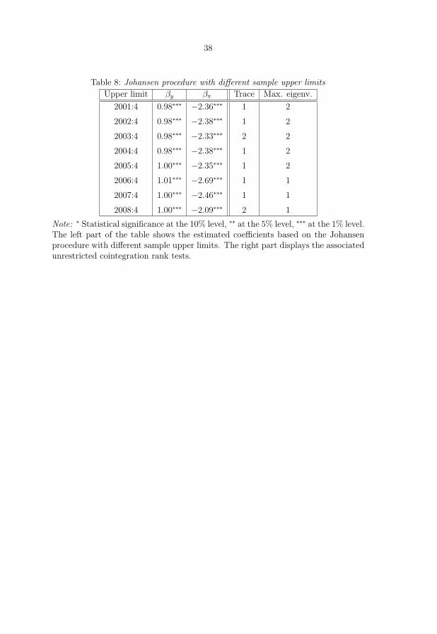
The performance and goodness-of-fit of all estimations conducted by us in this paperindicates that our estimation results for the euro area money demand are quiterobust. This is especially the case with respect to the estimated empirical realizationof the income elasticity. Hence, a remaining critical issue that arises in our contextis related to the stability of the estimated coefficients over time. In the ideal case,the stability tests should be conducted applying different methods in order to yieldrobust results.Accordingly, we start with the Johansen procedure and apply it in the same way asbefore in section 4.4, but this time sequentially letting the sample end after each yearfrom 2001 on in order to check whether the coefficient estimates stay the same. Welimit this exercise to the larger sample period, because we like to identify possibleeffects of events such as the burst of the so called dotcom-bubble in 2000, September11th in 2001 or the emergence of the global financial crisis in 2007. The short sampleunfortunately does not include enough observations to subdivide the sample periodand to still arrive at a sufficient number of degrees of freedom.


Our results in Table 8 indicate that there is some reason to consider the estimatedcoefficients of both regressors as stable over time. The results of the trace test andthe maximum eigenvalue test show that we can establish one or two cointegratingrelations between the five time series.

- Figures 1 and 2 about here -

Figures 1 and 2 display the identified cointegrating relations estimated with theJohansen approach alternatively for both sample periods. If the larger sample periodis used, coefficient stability turns out to be higher except for the change over (i.e.,after 1994:4) from the Coenen and Vega (1999) sample to ours.19

To check for stability of the coefficients, the latter are usually estimated in a recursivefashion. Hence, we proceed like this in case of our estimated ARDL model and19See the data description in section 4.1.

20

furthermore apply the cumulative sum (CUSUM) of squares test to both sampleperiods (Brown et al. (1975)).


According to Figures 3 and 4, the coefficients estimated based on the larger sampleperiod seem to be much more stable, except for the very beginning of the sample inthe early eighties.


However, the CUSUM of squares test surprisingly draws a quite different pictureand indicates some structural change in the larger sample. The empirical realizationof the CUSUM of squares test statistic falls outside the 5% significance bands formore than ten years (see Figures 5 and 6). Since previous tests do not support thisfinding, we could not definitely assume a structural break. There is particularly noindication of a structural break in the most interesting periods (2001 or 2007).

5. Robustness checks

To check for robustness of the estimated coefficients, three other cointegrating re-gression methods are applied as well as the Johansen framework and the ARDLapproach are used again while modifying the lag length. The findings of the latterare summarised in Table 9. Additionally, different model specifications are estimatedusing the cointegrated VAR approach with two lags for both samples as done beforein section 4.4.20

5.1. Other cointegrating regression methods

Hence, we also estimate the same specification by means of three other fully-efficientsingle equation cointegrating regression methods, namely the fully-modified OLS(FM-OLS) by Phillips and Hansen (1990), the canonical cointegration regression(CCR) by Park (1992) and the dynamic OLS (DOLS) by Saikkonen (1992) and Stockand Watson (1993). They have already been used by earlier studies for the purposeof estimating money demand functions,21 and will possibly be used in further studiesfor the euro area to put the achieved results of the above-mentioned techniques underscrutiny.20The Coenen and Vega (2001) (see pp. 728-729, 733-736) and the Brand and Cassola (2004)

specification (see pp. 818-819) are used. The results confirm our findings without improvingthe coefficient estimates. Nevertheless, they are not listed to save space, but they are availableupon request.

21See, for example, Calza et al. (2001), p. 30, Norrbin and Reffett (1997) and Mark and Sul (2003)in case of FM-OLS, CCR and DOLS, respectively.

21

5.1.1. Fully-modified OLS

The FM-OLS estimation procedure works with the standard triangular represen-tation of a regression specification and assumes the existence of a single cointe-grating vector (Phillips and Hansen (1990) and Hansen (1992)). Taking this as astarting point, we estimate the following cointegration equation based on a (d+ 1)-dimensional time series vector process [(m− p)t, X

′t]:

(m− p)t = X ′tβ +D′1tγ1 + u1t, (14)

where Dt = [D′1t, D′2t]′ are deterministic trend regressors and X ′

t =[yt, i

lt, i

st , πt

]rep-

resents d = 4 stochastic regressors, which are governed by the system of equations:

Xt = Γ′21D1t + Γ′22D2t + ε2t, (15)

with

Δε2t = u2t. (16)

In our case, the deterministic trend regressors D1t only contain a constant and enterboth the cointegrating equation and the regressors equations, while we include anyadditional deterministic trend regressors D2t in the regressors equations (15), butnot in the cointegrating equation (14).The FM-OLS estimator employs a semi-parametric correction to avoid estimationproblems caused by the long-run correlation between the cointegrating equation andstochastic regressors innovations. The resulting estimator is asymptotically unbiasedand has fully efficient mixture normal asymptotics allowing for standard Wald testsusing asymptotic χ2 statistical inference.Hence, the FM-OLS estimator is given by

θFMOLS =

[β

γ1

]=

(T∑

t=1

ZtZ′t

)−1( T∑t=1

Zt(m− p)+t − T

[λ+

12

′

0

]), (17)

where Zt = (X ′t, D

′t)′,

(m− p)+t = (m− p)t − ω12Ω−122 u2 (18)

represents the transformed data and

λ+12 = λ12 − ω12Ω

−122 Λ22 (19)

22

represents the estimated bias correction term with the long-run covariance matricesΩ and Λ (with their elements ω12, Ω22, λ12 and Λ22),22 which are computed usingthe residuals ut = (u′1t, u

′2t)′ (Hamilton (1994), pp. 613-618).

Our FM-OLS estimation based on the short sample period with the long-run co-variance estimates Ω and Λ applying a prewhitened kernel approach (with one lagaccording to SC) with a Bartlett kernel and Newey-West fixed bandwidth = 4.0000

leads to the following result:

(m− p)t = −5.78∗∗∗ + 1.16∗∗∗yt − 3.08∗∗∗ilt + 2.18∗∗∗ist − 2.08∗∗∗πt. (20)

What is more, using the longer sample period, the FM-OLS approach with long-runcovariance estimates using a non-prewhitened Bartlett kernel and a Newey-Westfixed bandwidth = 4.0000 yields the estimated cointegrating equation:

(m− p)t = −5.16∗∗∗ + 1.11∗∗∗yt − 1.91∗∗ilt + 1.80∗∗∗ist − 0.15∗πt. (21)

5.1.2. Canonical cointegration regression

The CCR estimation procedure is in principle closely related to FM-OLS, but insteademploys stationary transformations of the data to eliminate the long-run correlationbetween the cointegrating equation and stochastic regressors innovations. Hence,the CCR estimator is defined by

θCCR =

[β

γ1

]=

(T∑

t=1

Z∗t Z∗′t

)−1 T∑t=1

Z∗t (m− p)∗t , (22)

where Z∗t = (X∗′t , D

′t)′,

X∗t = Xt −

(Σ−1Λ2

)′ut (23)

and

(m− p)∗t = (m− p)t −(Σ−1Λ2β +

[0

Ω−122 ω21

])′ut (24)

represents the transformed data. The β’s are estimates of the cointegrating equationcoefficients applying static OLS, Λ2 is the second column of Λ and Σ represents theestimated contemporaneous covariance matrix of the residuals (Hamilton (1994),pp. 618-625).

22Lower case letters indicate in this case that elements are vectors and capital letters denotematrices.

23

Hence, applying the CCR procedure for the short sample period with long-run covari-ance estimates using the same kernel and Newey-West fixed bandwidth as appliedin the FM-OLS case yields the estimated money demand equation:

(m− p)t = −5.66∗∗∗ + 1.15∗∗∗yt − 3.07∗∗∗ilt + 2.4∗∗∗ist − 1.45∗∗πt. (25)

In contrast, the CCR estimation using the large sample period with long-run covari-ance estimates applying a non-prewhitening Bartlett kernel and a Newey-West fixedbandwidth = 4.0000 results in the following specification of the euro area moneydemand:

(m− p)t = −5.16∗∗∗ + 1.11∗∗∗yt − 1.84∗∗ilt + 1.82∗∗∗ist − 0.34∗πt. (26)

Seen on the whole, using both methods we come up with roughly the same coefficientestimates. Moreover, the latter are also in line with the predictions from theory andthe estimates within the Johansen and the ARDL framework. Furthermore, allcoefficients are significant and the estimates derived from the larger sample periodseem to be more appropriate since their magnitudes are even more striking accordingto the theoretical predictions and the previous empirical studies. Especially, thecointegrating equations which we derived from the larger data set explain the moneydemand in the euro area very well.The estimated income elasticity turns out to be positive and is nearly approachingunity. The estimated coefficients of the interest rate spread (ilt − ist) and the rate ofinflation which both approximate the opportunity costs of holding money prove tobe negative and relatively small.

5.1.3. Dynamic OLS

The DOLS estimation technique involves augmenting the cointegrating regression(14) with q lags and r leads of ΔXt such that the new cointegrating equation errorterm is orthogonal to the entire history of the stochastic regressor innovations:

(m− p)t = X ′tβ +D′1tγ1 +

r∑j=−q

ΔX ′t+jδ + v1t. (27)

However, the DOLS estimation procedure works under the assumption that theadded lags and leads of ΔXt completely eliminate the long-run correlation amongu1t and u2t. Hence, the resulting estimator is then given by θDOLS =

(β′, γ1

′)′

anddisplays the same asymptotic distribution as those derived with the FM-OLS andthe CCR estimation procedure.The DOLS approach using both sample periods with one lag and one lead and long-

24

run covariance estimates applying Bartlett kernel and Newey-West fixed bandwidth= 4.0000 delivers the following results:

(m− p)t = −8.69∗∗∗ + 1.35∗∗∗yt + 0.06ilt + 1.74∗∗∗ist − 3.21∗∗∗πt, (28)

and

(m− p)t = −5.19∗∗∗ + 1.11∗∗∗yt − 1.62∗∗ilt + 2.00∗∗∗ist − 1.06∗∗∗πt, (29)

respectively. Hence, the only difference in estimation results in comparison to theother methods used by us is the estimated semi-elasticity of the long-term interestrate. The latter does not turn out to be significant and displays the wrong sign forthe shorter sample period. Nevertheless, according to the Wald F -test, the jointeffect of the four variables on (m − p)t is highly significant in the case of all threecointegrating regression methods.23

5.2. Different lag lengths

Choosing the adequate lag length is always of interest when estimating VAR modelssince the underlying structure is often said to be atheoretic. As mentioned above,it is recommended in the literature to apply two lags as the adequate specificationin contexts like ours while using quarterly data. In our case, this choice is clearlysupported by the likelihood ratio, the final prediction error and the Hannan-Quinninformation criterion while setting the maximum lag length at a value of five. Nev-ertheless, the Akaike information criterion recommends five lags and the Schwarzinformation criterion points in favour of just one lag for the short sample period.However, the extension of the maximum lag length leads to different recommendedlag lengths. With an eye on the frequency of the data, it is also conceivable to applyfour lags. Hence, from this perspective it may be useful to check the estimationresults of our cointegrated VAR and ARDL specification dependent on using dif-ferent lag lengths for the large sample, whereas the small sample does not includeenough observations for such kind of an exercise. In the following, we proceed likethat and present the corresponding results in Table 9. Another possibility would beto estimate the ARDL model with different lag lengths for the endogenous and eachexogenous variable.


So, where do we get from here? First, most of the results in this section confirmthe above-mentioned findings especially with respect to the income elasticity, so23The results are available upon request.

25

that one could conclude by comparing the results of Table 9 and section 5.1 withthe ones in the previous sections 4.4 and 4.5 that our results are robust. Second,quite unsurprisingly, the larger sample period provides even more striking findingsaccording to related above-mentioned theoretical and empirical literature. Third,the modifications of the lag length do not produce better results than the initialmodels presented in the previous sections 4.4, 4.5 and 5.1.

6. Conclusion

In this contribution, we have shown that euro area money demand can be consideredas stable across different time periods. This result proves to be surprisingly robustto a battery of robustness checks. In fact, we have used two different sample sizeswhich allowed the conclusion that - just in line with Beyer (2009) - the ongoingfinancial and economic crisis has had no noticeable impact on the stability of euroarea money demand. Especially with respect to the income elasticity we come upwith very robust results independent of the specific estimation method applied.In a nutshell, we have pointed out that other efficient single equation methods be-yond the commonly used cointegration techniques such as the Johansen frameworkor the ARDL approach like the above-mentioned FM-OLS, CCR and DOLS couldbe helpful in estimating a statistically reliable money demand function. In viewof the remaining uncertainty surrounding the integration properties of the involvedvariables (I(0) or I(1)), single-equation techniques should be preferred. However,the amount of available euro area data might still be considered to be quite limited- at least as measured by the standards of asymptotic theory. Hence, one shouldstill make use of aggregated national data but inference should be drawn with ade-quate caution. This is the more valid since we have shown by comparing the resultsof both samples used for each technique applied that the more data we use in ourestimation exercises, the more the results are in line with the theoretical predictionsand the findings of previous empirical investigations.Finally, it should be also of interest to test for and estimate the cointegrating re-lation while augmenting the money demand equation with additional explanatoryendogenous and/or exogenous variables and introducing the identifying restrictionsfor that augmented variable set as well. We leave this task to future research.

26

References

Baharumshah, A. Z., S. H. Mohd, and A. M. M. Masih (2009): “The Sta-bility of Money Demand in China: Evidence from the ARDL Model,” EconomicSystems, 33 (3), 231–244.

Bahmani-Oskooee, M. and R. C. W. Ng (2002): “Long-Run Demand for Moneyin Hong Kong: An Application of the ARDL Model,” International Journal ofBusiness and Economics, 1, 147–155.

Baumol, W. J. (1952): “The Transactions Demand for Cash: An Inventory Theo-retic Approach,” The Quartely Journal of Economics, 66 (4), 545–556.

Belke, A. (2010): “Die Auswirkungen der Geldmenge und des Kreditvolumensauf die Immobilienpreise: Ein ARDL-Ansatz für Deutschland,” forthcoming:Jahrbuecher fuer Nationaloekonomie und Statistik.

Belke, A. and T. Polleit (2006a): “Dividend Yields for Forecasting Stock Mar-ket Returns: An ARDL Cointegration Analysis for Germany,” Ekonomia, 9 (1),86–116.

——— (2006b): “(How) Do Stock Market Returns React to Monetary Policy? AnARDL Cointegration Analysis for Germany,” Kredit und Kapital, 39 (3), 335–365.

——— (2006c): “Monetary Policy and Dividend Growth in Germany: Long-RunStructural Modelling versus Bounds Testing Approach,” Applied Economics, 38(12), 1409–1423.

——— (2009): Monetary Economics in Globalised Financial Markets, Springer-Verlag, Berlin Heidelberg New York.

Benati, L. (2009): “Long Run Evidence on Money Growth and Inflation,” EuropeanCentral Bank - Working Paper Series, No. 1027.

Bera, A. K. and C. M. Jarque (1981): “An Efficient Large-Sample Test for Nor-mality of Observations and Regression Residuals,” Australian National University- Working Papers Series in Econometrics, No. 40.

Beyer, A. (2009): “A Stable Model for Euro Area Money Demand - Revisiting theRole of Wealth,” European Central Bank - Working Paper Series, No. 1111.

Beyer, A., J. A. Doornik, and D. F. Hendry (2001): “Constructing HistoricalEuro-Zone Data,” The Economic Journal, 111, 102–121.

27

Boone, L. and P. van den Noord (2008): “Wealth Effects on Money Demandin the Euro Area,” Empirical Economics, 34 (3), 525–536.

Brand, C. and N. Cassola (2004): “A Money Demand System for Euro AreaM3,” Applied Economics, 36 (8), 817–838.

Brand, C., D. Gerdesmeier, and B. Roffia (2002): “Estimating the Trendof M3 Income Velocity Underlying the Reference Value for Monetary Growth,”European Central Bank - Occasional Paper Series, No. 3.

Brown, R. L., J. Durbin, and J. M. Evans (1975): “Techniques for Testing theConstancy of Regression Relationships Over Time,” Journal of the Royal Statis-tical Society, Series B, 37, 149–192.

Bruggeman, A., P. Donati, and A. Warne (2003): “Is the Demand for EuroArea M3 Stable?” European Central Bank - Working Paper Series, No. 255.

Calza, A., D. Gerdesmeier, and J. Levy (2001): “Euro Area Money Demand:Measuring the Opportunity Costs Appropriately,” IMF Working Paper Series,No. 01/179.

Calza, A. and J. Sousa (2007): “Why Has Broad Money Demand Been MoreStable in the Euro Area than in Other Economies? A Literature Review,” Kreditund Kapital, 1.

Carstensen, K., J. Hagen, O. Hossfeld, and A. S. Neaves (2009): “MoneyDemand Stability and Inflation Prediction in the Four Largest EMU Countries,”Scottish Journal of Political Economy, 56 (1), 73–93.

Chow, G. C. (1960): “Tests of Equality Between Sets of Coefficients in Two LinearRegressions,” Econometrica, 28 (3), 591–605.

Clausen, V. (1998): “Money Demand and Monetary Policy in Europe,” Review ofWorld Economics, 134 (4), 712–740.

Coenen, G. and J. L. Vega (1999): “The Demand for M3 in the Euro Area,”European Central Bank - Working Paper Series, No. 6.

——— (2001): “The Demand for M3 in the Euro Area,” Journal of Applied Econo-metrics, 16, 727–748.

De Santis, R. A., C. A. Favero, and B. Roffia (2008): “Euro Area MoneyDemand and International Portfolio Allocation - A Contribution to AssessingRisks To Price Stability,” European Central Bank - Working Paper Series, No.926.

28

Dedola, L., E. Gaiotti, and L. Silipo (2001): “Money Demand in the EuroArea: Do National Differences Matter?” Banca d’Italia - Discussion Paper Series,No. 405.

DeJong, D. N., J. C. Nankervis, N. B. Savin, and C. H. Whiteman (1992):“The Power Problems of Unit Root Tests in Time Series with AutoregressiveErrors,” Journal of Econometrics, 53, 323–343.

Dickey, D. A. and W. A. Fuller (1979): “Distribution of the Estimators forAutoregressive Time Series with a Unit Root,” Journal of the American StatisticalAssociation, 74, 427–431.

Dreger, C. and J. Wolters (2008): “M3 Money Demand and Excess Liquid-ity in the Euro Area,” DIW Berlin - German Institute for Economic Research -Discussion Paper Series, No. 795.

——— (2009): “Investigating M3 Money Demand in the Euro Area,” Journal ofInternational Money and Finance, 29 (1), 111–122.

ECB (2004a): “Monetary Analysis in Real Time,” Monthly Bulletin, October, 43–66.

——— (2004b): “The Monetary Policy of the ECB,” ECB 2nd ed.

Enders, W. (2010): Applied Econometric Time Series, Wiley, 3. edit. ed.

Engle, R. F. and C. W. J. Granger (1987): “Co-integration and Error Correc-tion: Representation, Estimation, and Testing,” Econometrica, 55, 251–276.

Engle, R. F., D. F. Hendry, and J.-F. Richard (1983): “Exogeneity,” Econo-metrica, 51 (2), 277–304.

Ericsson, N. R. (1999): “Empirical Modelling of Money Demand,” in Money De-mand in Europe, ed. by H. Lütkepohl and J. Wolters, Physica-Verlag, Heidelberg,29–49.

Fagan, G. and J. Henry (1998): “Long Run Money Demand in the EU: Evidencefor Area-Wide Aggregates,” Empirical Economics, 23 (3), 483–506.

Fair, R. C. (1987): “International Evidence on the Demand for Money,” The Reviewof Economics and Statistics, 69 (3), 473–480.

Faria, J. R. and M. A. León-Ledesma (2003): “Testing the Balassa-SamuelsonEffect: Implications for Growth and the PPP,” Journal of Macroeconomics, 25(2), 241–253.

29

Fase, M. M. G. and C. C. A. Winder (1998): “Wealth and the Demand forMoney in the European Union,” Empirical Economics, 23, 507–524.

Friedman, M. (1956): “The Quantity Theory of Money - A Restatement,” inStudies in the Quantity Theory of Money, ed. by M. Friedman, University ofChicago Press, 3–21.

Funke, M. (2001): “Money Demand in Euroland,” Journal of International Moneyand Finance, 20, 701–713.

Godfrey, L. G. (1978a): “Testing Against General Autoregressive and Moving Av-erage Error Models When the Regressors Include Lagged Endogenous Variables,”Econometrica, 46, 1293–1301.

——— (1978b): “Testing for Higher Order Serial Correlation in Regression Equa-tions When the Regressors Include Lagged Endogenous Variables,” Econometrica,46, 1303–1310.

Golinelli, R. and S. Pastorello (2002): “Modeling the Demand for M3 in theEuro Area,” The European Journal of Finance, 8, 371–401.

Gonzalo, J. and T.-H. Lee (1998): “Pitfalls in Testing for Long-Run Relation-ships,” Journal of Econometrics, 86, 129–154.

Greiber, C. and W. Lemke (2005): “Money Demand and Macroeconomic Un-certainty,” Deutsche Bundesbank - Discussion Paper Series 1, No. 26.

Greiber, C. and R. Setzer (2007): “Money and Housing - Evidence for the EuroArea and the US,” Deutsche Bundesbank - Discussion Paper Series 1, No. 12.

Halicioglu, F. (2004): “An ARDL Model of International Tourist Flows toTurkey,” Global Business and Economics Review 2004 Anthology, 614–624.

Hall, S. G., G. Hondroyiannis, P. A. V. B. Swamy, and G. S. Tavlas

(2008): “A Portfolio Balance Approach to Euro-Area Money Demand in a Time-Varying Environment,” University of Leicester, Department of Economics - Work-ing Paper Series, No. 08/9.

Hamilton, J. D. (1994): Time Series Analysis, Princeton University Press.

Hamori, S. and N. Hamori (2008): “Demand for Money in the Euro Area,”Economic Systems, 32 (3), 274–284.

Hansen, B. E. (1992): “Tests for Parameter Instability in Regressions with I(1)Processes,” Journal of Business and Economic Statistics, 10, 321–335.

30

Hansen, H. and S. Johansen (1999): “Some Tests for Parameter Constancy inCointegrated VAR-Models,” Econometrics Journal, 2, 306–333.

Harvey, A. C. (1976): “Estimating Regression Models with Multiplicative Het-eroscedasticity,” Econometrica, 44, 461–465.

Holtemöller, O. (2004): “A Monetary Vector Error Correction Model of the EuroArea and Implications for Monetary Policy,” Empirical Economics, 29, 553–574.

Issing, O., V. Gaspar, I. Angeloni, and O. Tristani (2001): Monetary Policyin the Euro Area, Cambridge University Press, Cambridge.

Johansen, S. (1988): “Statistical Analysis of Cointegration Vectors,” Journal ofEconomic Dynamics and Control, 12 (2-3), 231–254.

——— (1991): “Estimation and Hypothesis Testing of Cointegration Vectors inGaussian Vector Autoregressive Models,” Econometrica, 59 (6), 1551–1580.

——— (1995): Likelihood-Based Inference in Cointegrated Vector AutoregressiveModels, Oxford University Press.

Johansen, S. and K. Juselius (1990): “Maximum Likelihood Estimation andInference on Cointegration - With Applications to the Demand for Money,” OxfordBulletin of Economics and Statistics, 52 (2), 169–210.

Kelejian, H. H. (1982): “An Extension of a Standard Test for Heteroskedasticityto a Systems Framework,” Journal of Econometrics, 20, 325–333.

Kontolemis, Z. G. (2002): “Money Demand in the Euro Area: Where Do WeStand (Today)?” IMF Working Paper Series, No.02/185.

Lütkepohl, H. (2007): New Introduction to Multiple Time Series Analysis,Springer-Verlag, Berlin Heidelberg New York.

Lütkepohl, H. and J. Wolters, eds. (1999a): Money Demand in Europe,Physica-Verlag, Heidelberg.

Lütkepohl, H. and J. Wolters (1999b): “A Money Demand System for GermanM3,” in Money Demand in Europe, ed. by H. Lütkepohl and J. Wolters, Physica-Verlag, Heidelberg, 105–120.

MacKinnon, J. G. (1991): “Critical Values for Cointegration Tests,” in Long-Run Economic Relationships: Readings in Cointegration, ed. by R. F. Engle andC. W. J. Granger, Oxford University Press, chap. 13, 267–276.

31

——— (1996): “Numerical Distribution Functions for Unit Root and CointegrationTests,” Journal of Applied Econometrics, 11, 601–618.

MacKinnon, J. G., A. A. Haug, and L. Michelis (1999): “Numerical Distri-bution Functions of Likelihood Ratio Tests for Cointegration,” Journal of AppliedEconometrics, 14, 563–577.

Mark, N. C. and D. Sul (2003): “Cointegration Vector Estimation by PanelDOLS and Long-Run Money Demand,” Oxford Bulletin of Economics and Statis-tics, 65 (5), 655–680.

Müller, C. (2003): Money Demand in Europe: An Empirical Approach, Physica-Verlag, Heidelberg.

Morley, B. (2007): “Equities and the Monetary Model of the Exchange Rate: AnARDL Bounds Testing Approach,” Applied Financial Economics, 17, 391–397.

Narayan, P. K. and R. Smyth (2004): “Dead Man Walking: An EmpiricalReassessment of the Deterrent Effect of Capital Punishment Using the BoundsTesting Approach to Cointegration,” American Law & Economics AssociationAnnual Meetings, Berkeley Electronic Press, Paper 26.

Nautz, D. and K. Ruth (2005): “Monetary Disequilibria and the Euro/DollarExchange Rate,” Deutsche Bundesbank - Discussion Paper Series 1, No. 18.

Nicoletti-Altimari, S. (2001): “Does Money Lead Inflation in the Euro Area?”European Central Bank - Working Paper Series, No. 63.

Norrbin, S. C. and K. L. Reffett (1997): “The Disaggregated Money Demandin the Long Run,” Journal of Macroeconomics, 19 (3), 495–507.

Nyblom, J. (1989): “Testing for the Constancy of Parameters Over Time,” Journalof the American Statistical Association, 84, 223–230.

Park, J. Y. (1992): “Canonical Cointegrating Regressions,” Econometrica, 60, 119–143.

Payne, J. E. (2003): “Post Stabilization Estimates of Money Demand in Croatia:Error Correction Model Using the Bounds Testing Approach,” Applied Economics,35, 1723–1727.

Pesaran, M. H. and Y. R. Shin (1999): “An Autoregressive Distributed LagModelling Approach to Cointegration Analysis,” in Econometrics and EconomicTheory in the 20th Century: The Ragnar Frisch Centennial Symposium, ed. byS. Strom, Cambridge University Press, Cambridge, chap. 11, 371–413.

32

Pesaran, M. H., Y. R. Shin, and R. J. Smith (2001): “Bounds Testing Ap-proaches to the Analysis of Level Relationships,” in Special Issue in Honour ofJ D Sargan - Studies in Empirical Macroeconometrics, ed. by D. F. Hendry andM. H. Pesaran, Journal of Applied Econometrics, vol. 16, 289–326.

Phillips, P. C. B. and B. E. Hansen (1990): “Statistical Inference in Instru-mental Variables Regression with I(1) Processes,” Review of Economic Studies,57, 99–125.

Phillips, P. C. B. and P. Perron (1988): “Testing for a Unit Root in TimeSeries Regression,” Biometrika, 75, 335–346.

Ploberger, W., W. Krämer, and K. Kontrus (1989): “A New Test for Struc-tural Stability in the Linear Regression Model,” Journal of Econometrics, 40,307–318.

Ramsey, J. B. (1969): “Tests for Specification Errors in Classical Linear LeastSquares Regression Analysis,” Journal of the Royal Statistical Society, Series B,31, 350–371.

Saikkonen, P. (1992): “Estimation and Testing of Cointegrated Systems by anAutoregressive Approximation,” Econometric Theory, 8, 1–27.

Schwert, G. W. (1989): “Tests for Unit Roots: A Monte Carlo Investigation,”Journal of Business and Economic Statistics, 7, 147–159.

Sims, C. A. (1980): “Macroeconomics and Reality,” Econometrica, 48 (1), 1–48.

Stock, J. H. and M. Watson (1993): “A Simple Estimator of CointegratingVectors in Higher Order Integrated Systems,” Econometrica, 61, 783–820.

Tobin, J. (1956): “The Interest Elasticity of Transactions Demand for Cash,” TheReview of Economics and Statistics, 38 (3), 241–247.

Urbain, J.-P. (1992): “On Weak Exogeneity in Error Correction Models,” OxfordBulletin of Economics and Statistics, 54 (2), 187–208.

Warne, A. (2006): “Bayesian Inference in Cointegrated VAR Models with Applica-tions to the Demand for Euro Area M3,” European Central Bank - Working PaperSeries, No. 692.

Wesche, K. (1997): “The Stability of European Money Demand: An Investigationof M3H,” Open Economies Review, 8, 371–392.

33

——— (1998): Die Geldnachfrage in Europa - Aggregationsprobleme und Empirie,Physica-Verlag, Heidelberg.

White, H. (1980): “A Heteroskedasticity-Consistent Covariance Matrix Estimatorand a Direct Test for Heteroskedasticity,” Econometrica, 48 (4), 817–838.

Winder, C. C. A. (1997): “On the Construction of European-Wide Aggregates: AReview of the Issues and Empirical Evidence,” Irving Fisher Committee of CentralBank Statistics, IFC Bulletin, 1, 15–23.

34

A. Tables

Table 1: Literature surveyAuthor(s) Sample Money demand functionBeyer (2009) 80:1-07:4 (m− p)t = 1.7yt − 4.11hpit

Brand and Cassola (2004) 80:1-99:3 (m− p)t = 1.331yt − 1.61iltBrand et al. (2002) 80:1-01:2 (m− p)t = 1.34yt − 0.45iltBruggeman et al. (2003) 81:3-01:4 (m− p)t = 1.38yt − 0.81ist + 1.31iotCalza et al. (2001) 80:1-99:4 (m− p)t = 1.34yt − 0.86(ist − iot )

Carstensen et al. (2009) 79:4-04:4 (m− p)t = 0.994yt − 0.03iltClausen (1998) 80:1-96:4 (m− p)t = 0.98yt − 4.15ilt + 2.08istCoenen and Vega (2001) 80:4-98:4 (m− p)t = 1.125yt − 0.865(ilt − ist)− 1.512πt

Dedola et al. (2001) 82:1-99:4 (m− p)t = 1.38yt + 0.41(ist − iot )− 1.71(ilt − ist)

De Santis et al. (2008) 80:1-07:3 (m− p)t = 1.34yt − 0.76(ist − iot )

Dreger and Wolters (2009) 83:1-04:4 (m− p)t = 1.238yt − 5.162πt

Dreger and Wolters (2008) 83:1-06:4 (m− p)t = 0.955yt + 0.031yt ·D02Q1− 6.743πt

Fagan and Henry (1998) 80:3-93:4 (m− p)t = 1.59yt − 0.70ilt + 0.60istFase and Winder (1998) 72:1-95:4 (m− p)t = 0.66yt − 1.33ilt + 1.07ist − 1.33πt + 0.341wt

Funke (2001) 80:3-98:4 (m− p)t = 1.21yt − 0.3ist + 0.06D86

Golinelli/Pastorello (2002) 80:3-97:4 (m− p)t = 1.373yt − 0.68iltGreiber and Lemke (2005) 80:1-04:4 (m− p)t = −8.18 + 1.10yt − 2.43(ist − iot ) + 0.68unct

Greiber and Setzer (2007) 81:1-06:4 (m− p)t = 0.32yt − 2.55ilt + 0.84hpit

Holtemöller (2004) 84:1-01:4 (m− p)t = 1.275yt − 0.751iltKontolemis (2002) 80:1-01:3 (m− p)t = yt − 1.45istMüller (2003) 84:1-00:4 (m− p)t = 1.57yt − 2.22ilt + 1.87istWarne (2006) 80:2-04:4 (m− p)t = 1.38yt − 0.26(ist − iot )

Wesche (1997) 73:3-93:4 (m− p)t = 1.56yt − 2.40ilt

35

Table 2: Unit root testsVariable (m− p)t yt ist ilt πt

level t-stat. 3.54 −1.29 −2.92 −3.29 −5.49ADF level p-values 1.00 0.63 0.05∗ 0.02∗∗ 0.00∗∗∗

test Δ t-stat. −4.76 −3.38 −3.99 −5.17 −7.721995:1- Δ p-values 0.00∗∗∗ 0.02∗∗ 0.00∗∗∗ 0.00∗∗∗ 0.00∗∗∗

2009:2 level t-stat. 3.06 −1.51 −2.11 −3.79 −5.57PP level p-values 1.00 0.52 0.24 0.01∗∗ 0.00∗∗∗

test Δ t-stat. −4.78 −3.37 −4.04 −5.10 −12.90Δ p-values 0.00∗∗∗ 0.02∗∗ 0.00∗∗∗ 0.00∗∗∗ 0.00∗∗∗

level t-stat. 1.65 0.40 −1.37 −1.25 −9.54ADF level p-values 1.00 0.98 0.59 0.65 0.00∗∗∗

test Δ t-stat. −11.07 −9.85 −6.54 −6.01 −9.041980:1- Δ p-values 0.00∗∗∗ 0.00∗∗∗ 0.00∗∗∗ 0.00∗∗∗ 0.00∗∗∗

2009:2 level t-stat. 1.88 0.30 −1.02 −0.96 −9.74PP level p-values 1.00 0.98 0.74 0.77 0.00∗∗∗

test Δ t-stat. −11.07 −9.88 −6.46 −5.80 −103.33Δ p-values 0.00∗∗∗ 0.00∗∗∗ 0.00∗∗∗ 0.00∗∗∗ 0.00∗∗∗

Note: ∗ Statistical significance at the 10% level, ∗∗ at the 5% level, ∗∗∗ at the 1%level. For both tests the series contain a unit root under the null. Critical values aretaken from MacKinnon (1996): 10% −2.57, 5% −2.87, 1% −3.46. The test equationis estimated including an intercept. For the ADF test the number of lag is chosenby using the SC. Maximum lag number is 10 or 12 for the samples 1995:1-2009:2and 1980:1-2009:2, respectively. For the PP test autocovariances are weighted bythe Bartlett kernel.

Table 3: Lag length selection criteria - empirical realizations (1995:1-2009:2)Lag LogL LR FPE AIC SC HQ0 694.86 NA 2.06e− 18 −26.53 −26.35 −26.461 1076.21 674.70 2.31e− 24 −40.24 −39.11∗ −39.812 1112.81 57.72∗ 1.52e− 24∗ −40.69 −38.62 −39.90∗3 1134.27 29.71 1.87e− 24 −40.55 −37.55 −39.404 1162.54 33.71 1.90e− 24 −40.68 −36.74 −39.165 1194.29 31.75 1.88e− 24 −40.93∗ −36.06 −39.06

Note: An asterisk ∗ indicates the selected lag from each column criterion.

36

Table 4: Misspecification testsSample Test Stat. df p-value

LM(1) χ2 = 36.46 25 0.07∗

1995:1- LM(2) χ2 = 27.82 25 0.32

2009:2 Jarque-Bera χ2 = 15.16 10 0.13

White χ2 = 365.97 300 0.01∗∗∗

LM(1) χ2 = 18.20 25 0.83

1980:1- LM(2) χ2 = 18.24 25 0.83

2009:2 Jarque-Bera χ2 = 19351.72 10 0.00∗∗∗

White χ2 = 392.42 300 0.00∗∗∗

Note: ∗ Statistical significance at the 10% level, ∗∗ at the 5% level, ∗∗∗ at the 1%level.

Table 5: Unrestricted cointegration rank testSample Hypothesis Eigenvalues Trace-stat. 95% crit. v. p-value

r = 0 0.47 91.80 69.82 0.00∗∗∗

1995:1- r ≤ 1 0.40 57.20 47.86 0.01∗∗

2009:2 r ≤ 2 0.27 29.69 29.80 0.05∗

r ≤ 3 0.17 12.74 15.49 0.13

r ≤ 4 0.05 2.98 3.84 0.08

r = 0 0.23 82.59 69.82 0.00∗∗∗

1980:1- r ≤ 1 0.22 52.57 47.86 0.02∗∗

2009:2 r ≤ 2 0.10 24.49 29.80 0.18

r ≤ 3 0.08 12.89 15.49 0.12

r ≤ 4 0.03 3.63 3.84 0.06


37

Table 6: Likelihood ratio test of variable stationarity and weak exogeneity (95:1-09:2)Test (m− p)t yt ist ilt πt

χ2-stat. 4.40 5.09 5.04 5.17 1.57

Variable df 3 3 3 3 3

stationarity 95% critical value 7.82 7.82 7.82 7.82 7.82

p-value 0.22 0.17 0.17 0.16 0.67

χ2-stat. 5.70 3.54 7.11 6.49 18.03

Weak df 2 2 2 2 2

exogeneity 95% critical value 5.99 5.99 5.99 5.99 5.99

p-value 0.06∗ 0.17 0.03∗∗ 0.04∗∗ 0.00∗∗∗


Table 7: Residual testsSample Test Test-statistic p-value

Breusch-Godfrey F (2, 38) = 1.17 0.32

1995:1- Harvey F (14, 40) = 0.43 0.95

2009:2 Jarque-Bera χ2(2) = 2.50 0.29

Ramsey F (1, 39) = 3.63 0.06∗

Breusch-Godfrey F (2, 98) = 1.47 0.24

1980:1- Harvey F (14, 100) = 0.43 0.13

2009:2 Jarque-Bera χ2(2) = 54.04 0.00∗∗∗

Ramsey F (1, 99) = 0.22 0.64

Note: ∗ Statistical significance at the 10% level, ∗∗ at the 5% level, ∗∗∗ at the 1%level. Ramsey’s RESET test is applied using squared residuals.

38

Table 8: Johansen procedure with different sample upper limitsUpper limit βy βπ Trace Max. eigenv.

2001:4 0.98∗∗∗ −2.36∗∗∗ 1 2

2002:4 0.98∗∗∗ −2.38∗∗∗ 1 2

2003:4 0.98∗∗∗ −2.33∗∗∗ 2 2

2004:4 0.98∗∗∗ −2.38∗∗∗ 1 2

2005:4 1.00∗∗∗ −2.35∗∗∗ 1 2

2006:4 1.01∗∗∗ −2.69∗∗∗ 1 1

2007:4 1.00∗∗∗ −2.46∗∗∗ 1 1

2008:4 1.00∗∗∗ −2.09∗∗∗ 2 1

Note: ∗ Statistical significance at the 10% level, ∗∗ at the 5% level, ∗∗∗ at the 1% level.The left part of the table shows the estimated coefficients based on the Johansenprocedure with different sample upper limits. The right part displays the associatedunrestricted cointegration rank tests.

39

Table 9: Johansen procedure and ARDL approach with different lag lengths

Lags Money demand function χ2(2)-statistic p-value1 (m− p)t = −3.32 + 0.99∗∗∗yt − 3.02∗∗∗πt 14.67 0.00∗∗∗

3 (m− p)t = −3.83 + 1.02∗∗∗yt − 1.12∗∗∗πt 12.06 0.00∗∗∗

4 (m− p)t = −3.64 + 1.01∗∗∗yt − 1.28∗∗∗πt 12.63 0.00∗∗∗

5 (m− p)t = −3.65 + 1.01∗∗∗yt − 1.37∗∗∗πt 13.89 0.00∗∗∗

6 (m− p)t = −3.97 + 1.03∗∗∗yt − 1.07∗∗∗πt 5.02 0.08∗

7 (m− p)t = −4.06 + 1.03∗∗∗yt − 0.93∗∗∗πt 13.57 0.00∗∗∗

8 (m− p)t = −6.47 + 1.19∗∗∗yt + 8.53∗∗∗πt 10.69 0.01∗∗∗

Lags Money demand function F -stat. (df) p-value3 (m− p)t = 1.25∗∗yt + 5.78∗∗∗ist − 4.82∗∗ilt − 1.52πt 2.67 (5, 94) 0.03∗∗

4 (m− p)t = 1.21∗yt + 4.93∗∗ist − 4.27∗ilt − 0.98πt 1.54 (5, 88) 0.19

5 (m− p)t = 1.19yt + 8.10∗ist − 9.28∗ilt + 0.47πt 1.38 (5, 82) 0.24

6 (m− p)t = 1.95yt + 25.39ist − 26.19ilt + 3.88πt 0.93 (5, 76) 0.47

7 (m− p)t = 1.09yt + 7.70ist − 11.28ilt + 2.77πt 1.08 (5, 70) 0.38

8 (m− p)t = 0.83yt + 12.91ist − 22.45∗ilt + 7.27πt 1.76 (5, 64) 0.14

Note: ∗ Statistical significance at the 10% level, ∗∗ at the 5% level, ∗∗∗ at the 1%level. The upper part of the table shows the estimated money demand functionsbased on the Johansen procedure with different lag lengths and the lower part thesame based on the ARDL approach. The Johansen procedure is applied with r = 2.The LR test is used to check within the Johansen framework whether to reject theimposed restrictions or not. In case of the estimations based on the ARDL approach,the null of no cointegration is tested by means of the Wald F -test.

40

B. Figures

Figure 1: Cointegration relations (1995:1-2009:2)

Note: The figure shows the cointegrating equations (5) and (6) for the euro area es-timated based on the Johansen procedure. They can be interpreted as the euro areamoney demand equation (left-hand side) and an equation combining the term struc-ture of interest rates and the Fisher inflation parity (right-hand side), respectively,for the short sample (1995:1-2009:2).

Figure 2: Cointegration relations (1980:1-2009:2)

Note: The figure shows the cointegrating equations (8) and (9) for the euro areaestimated based on the Johansen procedure. They characterize the money demand(left-hand side) and an equation combining the term structure of interest rates andthe Fisher inflation parity (right-hand side) for the large sample (1980:1-2009:2).

41

Figure 3: Recursive estimates of the coefficients of the ARDL model (1995:1-2009:2)

Note: The figure shows one after the other the recursive estimates of the coefficientsof the ARDL model γ0, γ1, γ2, γ3 and γ4 (see equation (11)) for the short sample(1995:1-2009:2).

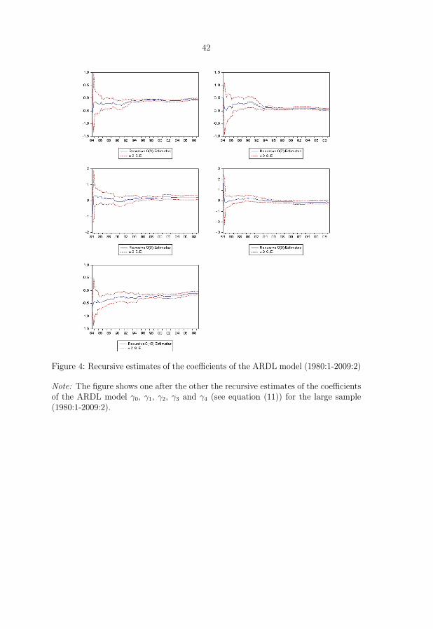
42

Figure 4: Recursive estimates of the coefficients of the ARDL model (1980:1-2009:2)

Note: The figure shows one after the other the recursive estimates of the coefficientsof the ARDL model γ0, γ1, γ2, γ3 and γ4 (see equation (11)) for the large sample(1980:1-2009:2).

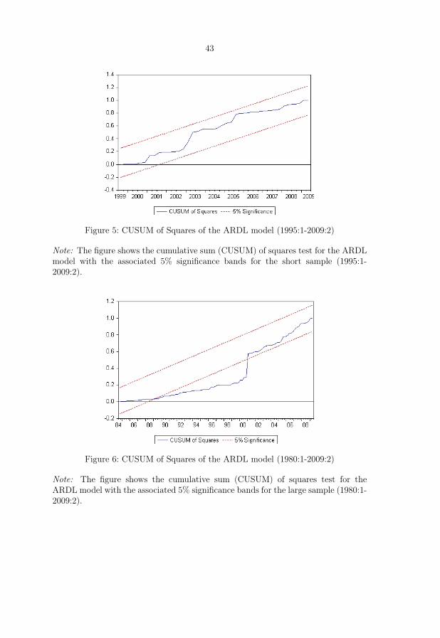
43

Figure 5: CUSUM of Squares of the ARDL model (1995:1-2009:2)

Note: The figure shows the cumulative sum (CUSUM) of squares test for the ARDLmodel with the associated 5% significance bands for the short sample (1995:1-2009:2).

Figure 6: CUSUM of Squares of the ARDL model (1980:1-2009:2)

Note: The figure shows the cumulative sum (CUSUM) of squares test for theARDL model with the associated 5% significance bands for the large sample (1980:1-2009:2).

Date post:	23-Apr-2018
Category:	Documents
Upload:	vuquynh
View:	217 times
Download:	0 times

Euro area money demand - Empirical investigation using a ... · Prof. Dr. Christoph M. Schmidt RWI,...

Documents