EUROPEAN ECONOMY EUROPEAN COMMISSION DIRECTORATE-GENERAL FOR ECONOMIC AND FINANCIAL AFFAIRS ECONOMIC PAPERS ISSN 1725-3187 http://europa.eu.int/comm/economy_finance Number 229 July 2005 The dynamics of regional inequalities by Salvador Barrios * and Eric Strobl ** * Directorate General for Economic and Financial Affairs and ** Ecole Polytechnique, Paris
Transcript
EUROPEAN
ECONOMY
EUROPEAN COMMISSION DIRECTORATE-GENERAL FOR ECONOMIC
This paper analyses empirically the dynamics of regional inequalities in GDP per capita. Our starting hypothesis is that the evolution of regional inequalities should follow a bell-shaped curve depending on the level of national economic development. A number of authors going from Kuznets (1955) to Lucas (2000) have provided extensive theoretical arguments along this line suggesting that growth, because of its very nature, is unlikely to appear everywhere at the same time. Regional inequalities should then rise when countries start developing and then fall once a certain level of national economic development is reached as long as spillovers are strong enough to transmit growth and technological progress across regions. We test empirically these predictions by using regional data for a panel of European countries and by making use of semi-parametric estimation techniques. Our results provide strong support for a bell-shaped curve in the relationship between the national GDP per capita level and the extent of regional inequalities independently of the time period and regional administrative units considered. The nature of this non-monotonic relationship is not altered by the inclusion of other possible determinants of regional inequalities. A number of policy implications are derived from our results. JEL classification: R1, R5, D31 Keywords: Kuznets curve, economic development, regional inequalities, Europe * Many thanks to Manfred Bergmann, Luisito Bertinelli, Fabio Canova, Bruno Cruz, Enrique Lopez Bazo, Carole Garnier, Stefano Magrini, Mario Maggioni, Diego Martinez, Yasuhiro Sato, Antonio Teixeira and Jacques Thisse as well as participants to the CentrA workshop held in Seville, economic seminar at the University of Nottingham and CEPR workshop in Cagliary for very helpful comments. We are particularly indebted to Martin Hallet for excellent comments and suggestions. Also many thanks to Paul Cheshire for providing us the Functional Urban Areas data and Jim McKenna for help with the European data. We also wish to thank Dana Weist and Ines Kudo for providing us the World Bank data on fiscal decentralisation. The views expressed by the authors are not necessarily those of the institutions they are affiliated with. a Corresponding author, Email: [email protected]. A previous version of this paper was circulated under the title: “Revisiting the link between national development and regional inequalities: Evidence for Europe”.
Economists have increasingly paid attention to the role played by knowledge and spillovers
in explaining countries’ growth differentials and diffusion both across countries and regions, see,
for instance, Jones (2004) and Klenow and Rodriguez-Clare (2004). Accordingly, knowledge
spillovers should give rise to substantial scale effects in productivity stemming from their non-
rivalry nature.1 However, although knowledge and technological progress are in this regard seen as
the main engines of economic development, the latter may inevitably increase rather than decrease
regional inequalities since these two elements are very unlikely to be evenly spread both across time
and space. As a consequence, economic growth may, at least initially, foster divergence, rather than
convergence across spatial units suggesting that convergence may evolve non-linearly. Indeed,
when considering the theoretical literature on growth and convergence, a wide array of arguments
arise advocating either for the long-term reduction or, to the contrary, for the persistence and self-
reinforcing nature of economic inequalities across countries and regions, see, for instance, Galor
(1996), Prichett (1997) and Lucas (2000). Elements such as spillover effects and nonlinearities have
also been considered in empirical studies providing growing evidence for the non-linear nature of
the growth and convergence processes, see, for instance, Durlauf and Johson (1995), Liu and
Stengos (1999), Quah (1996b, 1997) and Canova (2004).
Interestingly, the idea that regional inequalities are likely to evolve in a nonlinear way can
be traced back as early the 1950s. The evolution of regional inequalities was then usually linked to
national economic development paths. As a matter of fact, it was Kuznets (1955) in his analysis of
income disparities who suggested the existence of a “long swing” in regional income inequalities,
where there was first a rise and then a subsequent fall of income differentials caused by the
urbanization and industrialization process accompanying national development and the decline of
agriculture. Several authors have built on this idea for regional analysis suggesting the existence of
a bell-shaped curve of spatial development where inequalities should first rise as developed areas
- 4 - 1 This is a central theme in the works of Romer (1990), Kremer (1993) and Tamura (1996) among others.
benefit from external economies, location of decision-makers, political power and capital and
labour mobility, see for instance Myrdal (1957), Hirschman (1958), Williamson (1965) and, more
recently, Ottaviano and Thisse (2004).2
While a non-linear relationship between regional inequality and national development
clearly has important implications for economic theory and policy, there is to the best of our
knowledge no explicit econometric study that has set out to investigate its existence, although a
number of works have been suggestive of its possibility. In the current paper we explicitly test for
the possibility of a non-linear relationship link between national development and regional
inequalities using data for EU countries. The EU economy makes arguably for a particularly
suitable case study given the sizeable disparities in economic development both across regions and
countries, compared to, for instance, the US. One may thus exploit the fact that these countries are
on very different positions on their development path, hence allowing one to observe regional
inequality across a wide range of economic development levels. To investigate this we use data on
GDP per head for European regions between 1975 and 2000. We show using a flexible semi-
parametric estimator that the relationship between national GDP per head and regional inequalities
follows a bell-shaped curve, suggesting that growth first increases regional inequalities but then
tends to lower them as the national level of income continues to rise. This result is robust to
considering other OECD countries, alternative geographical units, and after controlling for other
potential determinants of regional inequalities such as the degree of international openness,
industrial specialization, regional aid, and the level of fiscal decentralization. Our paper is thus, to
the best of our knowledge, the first study to provide robust evidence of the bell-shaped relationship
between regional inequalities and national economic development.
The remainder of the paper is organized as follows. In Section 2 we review the existing
empirical literature concerning the link between national development and regional inequalities. In
this section we also present a simple theoretical model to illustrate the main mechanisms at hand.
- 5 -
2 The evidence concerning the non-linear relationship between urbanization and development is also a well documented fact in urban economics, see, for instance, the seminal work of Alonso (1969).
Sections 3 and 4 present some preliminary evidence and our main econometric results. Section 5
summarises our findings and discusses some policy implications.
2. Revisiting the link between national development and regional inequalities
2.1 Related empirical literature
A number of empirical artefacts tend to support the possibility of a bell shaped relationship between
regional inequality and national development. Following the footsteps of Kuznets (1955),
Williamson (1965) provides an extensive analysis on the topic by analyzing in details the spillovers
mechanism driving the evolution of regional inequalities according to the stages of development of
a nation. According to Williamson (1965), spillovers may occur through a number of channels such
as migration, capital flows, government policy and interregional trade. Using evidence based on
descriptive statistics for a number of countries between the end of the XIXth Century and World
War II, he found some supportive evidence for a non-linear relationship between regional
inequalities and national development. His conclusions derive from two main empirical facts: first,
regional disparities are greater in less developed countries and smaller in the more developed ones;
second, over time, regional disparities increase in the less developed countries and decrease in the
more developed. Accordingly, regional income inequalities can be considered as a by-product of the
development process of a nation and any attempts at lowering them may eventually hamper this
process. Kim and Margo (2003) also show that in the US the rise of industrialization during the
second half of the nineteenth century has increased regional income disparities, where
manufacturing was concentrated in the North and specialization in agricultural activities occurs in
the South. By the second half of the twentieth century, however, regional industrial structures
converged through a dispersal of agriculture and the rise of services activities across the US States.
More recently, in the European context, De la Fuente and Vives (1995) have noted that the
European integration process may drive regions located in the same country to divergence in
income per capita. Quah (1996a) also observes that the two countries that have reached the highest
rates of economic growth, Spain and Portugal, are those that have experienced the most striking rise
- 6 -
in regional imbalances. In another contribution, Quah (1999) considers the case of three EU
cohesion countries, Spain, Portugal and Greece, and shows that while the first two have experienced
strong growth rates and growing regional imbalances during the 1980-89 period, Greece has
experienced only modest growth rates accompanied by decreasing income inequalities across its
regions.3 Petrakos and Saratis (2000) also find similar evidence for Greece. These authors find that,
during the 1980s, the most developed regions in Greece have faced growing difficulties due to
tighter foreign competition implied by the European integration process, while less developed
regions were less affected. Petrakos and Saratis (2000) also argue that this may be one of the
reasons explaining why regional inequalities have tended to decrease in this country during the
1980ies. In more recent contributions, Davies and Hallet (2000) together with Petrakos et al. (2003)
consider more closely the possibility of a bell-shaped curve in regional inequalities for the EU. The
former study is essentially descriptive and finds some evidence for growing regional income
imbalances for the poorest EU countries while the latter tests econometrically the link between
regional inequalities and the level as well as the growth rate of national GDP. However, Petrakos et
al. (2003) only allow for GDP level to have a linear effect, which is unlikely to capture the bell-
shaped curve of spatial development. This point will be further developed in Section 3. Before
presenting our econometric results it is worth setting the basic mechanics underlying the non-linear
relationship between regional inequalities and national economic development.
2.2 A simple model of growth, catching-up and technological diffusion
The model presented here is derived from Lucas (2000) where spillovers are the main vehicle of
economic development. This author does not directly deal with the relationship between regional
inequalities and national development. His model can, however, be used in order to see how growth
transition dynamics can influence the evolution of regional inequalities. Let us consider a country
composed by a number n of regions. Initially all regions are supposed to have a constant level of
income per capita y0. Now let us consider that growth occurs in only one region at date t=0. By
3 The group of Cohesion countries here refers to the countries entitled to the so-called EU Cohesion fund including, for the period considered here, Ireland, Greece, Portugal and Spain. The Cohesion fund is aimed at favouring economic
- 7 -
making this hypothesis we assume that growth is, at least initially, localized. The other regions will
start growing at date s>0 and each region starts growing at a different date. In making this
assumption, we assume that regions differ in their technological capability. The model thus implies
a distribution of starting dates characterising regional differences in technological capability. We
can thus index regions by the date at which they start growing such that y(s,t) will be the income per
capita level of a region s which starts growing at a date t=s. The level of income of the innovative
region at any date t can thus be written as y(0,t) such that:
( ) ( )tyty α+= 1,0 0 (1)
where α is the steady state growth rate of the leading region and y0 its initial level of income. When
the other regions start growing at a date t>0, they do so according to the following expression:
βα )),(),0(()1(
),()1,(
tsyty
tsytsy
+=+ (2)
where β is a catch-up rate that we assume to be constant for all the (followers) regions. This term
represents the spillover effect described earlier. The starting hypothesis is that, once the leading
region starts growing, as time passes and average national income grows, the probability for any
region to switch from stagnation to growth will rise and follow a cumulative process. Put
differently, the larger the number of existing regions that are in a growth regime, the higher the total
amount of knowledge and technological capability available in the economy and the higher the
probability for any other region to get access to this knowledge and to start growing. Let consider
the (unconditional) probability F(t) that any of such region starts growing at date t. 4 The average
level of income of this economy can thus be described as a weighted sum of the level of income of
each region-type, i.e., growing and stagnating regions, as follows:
0)(1),()()( ysFtsysFtxtsts
−+= ∑∑≤≤
(3)
development of countries with a level of GDP per capita below 90% of the EU average.
- 8 -
4 The hazard rate is given by λ(t) = λ and the corresponding survival rate function is such that the probability F(t) that any region starts growing at a date t can be derived in the usual way from the hazard rates model such that
tt eS λ−=
( ) ( )
−= ∑< ts
sFttF )(1λ
where the probabilities of being in a growth regime or stagnation regime are used as weights. Using
this expression, the extent of regional inequalities can be, as in Lucas (2000), described by log
standard deviation of income across regions σ(t) such that:
2
0
2
2
)(ln)(1
)(),(ln)()(
−+
= ∑∑
≤≤ txysF
txtsysFt
tsts
σ (4)
and can be seen as the weighted value of the standard deviation of regional GDP per capita. Figure
1 depicts the relationship between the average level of income (or national average of income per
capita) and σ(t).5 According to this figure, the relationship between the level of regional inequalities
and the per capita national income level is non-monotonic and follows a bell-shaped curve.
Regional inequalities initially rise as long as the forces for divergence dominate while, after a
certain threshold which depends on the level of development of the national economy, regional
inequalities start falling. The latter occurs because the probability for a region to be in a growth
regime increases while the probability of being in a stagnation regime declines as time goes on and
national average income rises. Therefore, a larger country-wide stock of knowledge, or,
equivalently, a higher level of average income, improves the level of technology (i.e., the level of
income) of each region. The model of economic growth presented here is thus purely a model of
technological diffusion where the number of regions benefiting from technological progress rises as
the total amount of knowledge in the country increases. One must reckon, however, that the
diffusion of growth described by equation (2) looks very much like a black box. The model thus
does not rule out, the fact that other mechanisms could as well explain growth transmission across
regions. As noted by Lucas (2000), one could as well assume that such spillovers may occur
through human capital externalities (Tamura, 1996), through institutions and the removal of barriers
to technology adoption such as regulatory or legal contraints as argued by Parente and Prescott
(1994), or simply through factor mobility and non-constant returns to capital as in Solow (1956).
The identification of these alternative explanations goes beyond the scope of the present study. Here
we rather try to assess whether the relationship depicted by Figure 1 holds for different samples of
- 9 -
European countries. One feature of EU economies, is the existing huge levels of income disparities
both across regions and countries compare to the US, for instance. The latter means that, by
observing the evolution of regional inequalities and level of national economic development and
considering all countries/regions together across time one may be able to analyse transition
dynamics in regional inequalities. This would amount to consider that any point on the curve plotted
in Figure 1 corresponds to the relative values of income per capita and level of regional inequalities
of a given country at any date t.
3. Data and Preliminary evidence
3.1 Data and measure of regional inequalities
We use data on Gross value added per capita by NUTS2 regions using the Cambridge
econometrics database which is based on Eurostat data, see Table A1 in Appendix for further details
on the number of regions covered by country.6 Despite the fact that most studies on EU regions use
this regional breakdown, an issue with the NUTS2 regional breakdown is that these regions are not
economically homogenous. The consequence is that the geographical definition of regions NUTS2
may sometimes be artificial in order to comply with European standards. For this reason, in section
4 we will use alternative datasets and definition of spatial units in order to check the robustness of
our results. The level of national development is represented by the GDP per capita expressed in
Purchasing Power Standards (PPS) with one unit of PPS representing approximately one euro.7 Our
measure of regional inequalities is the standard deviation of the logarithm of the GDP per capita
following the model presented in Section 2. A number of alternative indicators could have been
considered such as the Gini index although one must note that the results obtained with these other
possible measures are in line with the ones presented here.8 Note that the use of logarithm of GDP
per capita reduces the potential bias related to the mechanical link between the evolution of the
5 Values of the parameters used for the numerical examples are given in the Appendix. 6 Note that we systematically checked the results obtained using the Cambridge Econometrics data by using the regio database which is less complete. The results obtained were nearly identical to the ones presented here. 7 Table A1 in Appendix provides further details concerning the countries considered and the number of observations available for the different datasets used in the paper.
- 10 -
national GDP and its regional component. For instance, for a given level of population, one can
well imagine that variations in the level of all regions GDPs may artificially imply a rise in the
absolute inequality. The use of natural logarithm of the GDP per head tends to lower this potential
effect. In addition, as usual in the growth literature, our GDP per capita variables are measured
relative to the EU average. This allows us to reduce both serial correlation and the effect of
potential outliers, see Canova (2004).
3.2 Preliminary evidence
According to the existing evidence for Europe, the poorest EU members have experienced
fast catching-up over the past two decades or so and this has translated into rising regional
inequalities. In order to provide further evidence on this, we first consider the EU15 countries for
which we have the longest time series. More specifically, we consider first the countries which, at
the start of the period, had the lowest level of GDP per capita, namely, Greece, Portugal and Spain.
Lack of sufficiently disaggregated data at the regional level for Ireland does not allow including
evidence for this country despite the fact that Ireland also benefited from the EU Cohesion fund.
Table 1 displays the level of national GDP and the standard deviation of regional GDP per capita
for these countries. The level of regional inequalities appears to be, on average and for most of the
period considered here, higher in the Cohesion country group compared to the rest of the EU. This
distinctive feature also holds when considering Cohesion countries individually, except for Greece,
which is also the EU15 country with the lowest GDP per capita. One must note, however, that it is
rather difficult to draw any conclusive evidence concerning the evolution of regional inequalities
given that this indicator is rather volatile, especially, but not exclusively, for the cohesion country
group as shown in Table 2. Despite this, we can still identify two distinct periods concerning the
evolution of regional inequalities and convergence in the Cohesion countries. The first is the 1975-
1985 period, marked by slow economic growth in the EU as a whole, and declining regional
inequalities in Spain, Greece and Portugal. By contrast, the following two periods were
- 11 -
8 Note also that, in order to check whether the standard deviation of regional GDP per capita was influenced by the number of regions by country, we computed correlation these two variables for the EU15 and it was equal to –0.33.
characterized by fast catching-up and rising regional inequalities. These two periods are also
marked by the accession of two cohesion countries in 1986, namely Spain and Portugal, with initial
GDP per capita much lower than the EU15 average. During 1986-1992 income per capita
converged steadily in Portugal and Spain together with a rise in regional income inequalities. In
Greece, however, the slight decline in income per capita relative to the EU average was
accompanied by a rise in regional inequality compared to the rest of the EU but remaining at levels
well below the EU average. The period 1992-2000 is characterized by a rather stable level of
regional inequalities in Spain and rising inequalities in Greece and Portugal. This rise, in turn,
corresponds to a rapid convergence of GDP per capita for the last two countries.
The evidence regarding the rise in regional inequalities that accompanies national economic
development is even more pronounced when considering the countries that joined the EU in 2004.
Table 3 provides detailed statistics for these and shows that, as for the Cohesion countries, these
countries display, on average, higher regional inequalities than the EU15 countries, including the
Cohesion countries. In addition, they have almost invariably all experienced a continuous increase
in the level of regional inequalities during the period 1995-2000, except Bulgaria, Poland and
Slovenia. While part of this evolution is probably due to the transition from a planned to a market-
oriented economy, most of the impact of this process at the regional level was experienced in the
early 1990s. It follows that a large part of the rise in regional imbalances is likely to be due to the
rapid catching-up process experienced by these countries during the past decade as shown by
Petrakos et al. (2000). However, not all countries have been catching-up during the 1995-2000
period. Countries such as Bulgaria, the Czech Republic and Romania have even seen the level of
their GDP per capita compared to the EU15 average decline during these years. On average, these
countries have also experienced a less pronounced rise in regional inequalities.9 One must reckon
that these preliminary results face some limitations. First, one needs to further check whether non-
observable country-specific features influence the nature of this relationship. Second, as mentioned
9 This can be seen by splitting the Eastern European countries considered here into two samples, those that have caught-up and those that have not. If one considers weighted average (using country-level population as weight), the non
- 12 -
earlier, regional inequalities have not only risen in the poorest EU countries but also in some of the
richest ones. It follows that the non-linear relationship between economic development and regional
inequalities is hard to detect from the descriptive statistics presented above. The existing evidence is
essentially focused on the ascending part of the bell-shaped curve (i.e. increasing disparities in
poorer countries) while much less evidence is available concerning the descending part (i.e.
decreasing disparities in richer countries). Part of the reason for this may be due to the fact that the
processes underlying the descending part might be less automatic than for the ascending part and
much more depending on pro-active regional policy and/or on implicit redistribution schemes. The
evidence for Europe suggests that these policy-related factors play an important role in smoothing
income inequalities in some countries such as Germany or France, for instance, see European
Commission (2000) and OECD (2004). In order to go a step further in the analysis, the next section
provides econometric result based on parametric and semi-parametric methods.
4. Econometric Analysis
4.1 Econometric methodology
In this section we present the econometric methodology used to study the relationship
between the level of economic development represented by the relative (to the EU) level of GDP
per capita (that we call Y) and the relative (to the EU) level of regional inequalities, represented by
X, both variables being observed at the country-level. Following our underlying hypotheses, the
level of economic development of a country should explain where this country lies in terms of
regional inequalities with poorer countries experiencing growing regional imbalances as they catch
up with richer countries. One way to test econometrically the relationship between Y and X is to run
a simple parametric OLS estimation including both country and time dummies to control for
country specific time invariant unobservables and time specific factors common to all countries in
the sample. An example of the results obtained with such method can be provided by using, for
instance, the data concerning the EU15 regions over the 1975-2000 period. We include both the
- 13 -
catching-up countries have seen the level of regional inequalities to increase by around 21% while the catching-up countries have more than doubled this figure with a rise equal to 43%.
level of national GDP per capita and its square-term in order to capture the non-linear relationship
described earlier. The results of running the parametric estimations are given in the first column of
Table 4. As can be seen, our results suggest that national prosperity acts to decrease regional
inequalities while the square value of this variable is insignificant. However, a simple Ramsey
RESET test suggests that the specified functional form may not be correct. We also experimented
with other higher order terms of the national GDP per capita but were unable to obtain a RESET
test statistic that did not suggest misspecification.10 One problem, of course, with simply using
higher order terms to estimate a possibly non-linear relationship is that even these place fairly
strong restrictions on the possible link between the dependent variable and the explanatory variable
of interest that may not reflect the true underlying relationship. A more flexible approach to tackle
non-linearity issues in growth and convergence studies is to use semi-parametric methods, as
suggested by Durlauf (2001). In this way one can investigate the possible non-linearity of the
relationship between regional inequality and national development, while also allowing for the
(linear) effect of other conditioning variables. We follow the semi-parametric methodology
proposed by Robinson (1988) using the Kernel regression estimator.11 Accordingly, one can
consider the following equation to be estimated:
Y = α + g(X) + δZ + u (5)
where Z are a set of explanatory variables that are assumed to have a linear effect on Y, g(.) is a
smooth and continuous, possibly non-linear, unknown function of X, and u is a random error term.
Robinson’s methodology proceeds in two steps. First, an estimator of δ, ,can be obtained by using
OLS on:
δ
Y – E(Y|X) = δ [Z – E(Z|X) ] + v (6)
10 The result of the RESET test when including the level of national GDP only displays a F-value equal to 10.84 and significant at 1%. When including this variable and its squared term the F-test value is 8.18 and is also significant at 1%.
- 14 - 11 See Blundell and Duncan (1998) for details and a helpful discussion of the implementation of this method.
Where v satisfies E(v|X,Z) = 0 and E(Y|X) and E(Z|X) are estimated using the Nadaraya-Watson
non-parametric estimator. For instance, the estimation of E(Y|X), ( )XmYˆ , can be written as 12
(XmYˆ )= ∑
∑
=
=
−
−
n
iih
n
iiih
XxK
YXxK
1
1
)(
)(i
(7)
such that i=1…n are the n number of observations, Kh() is the shape function, commonly referred to
as the Kernel, that is a continuous, bounded and real function that integrates to one and acts as a
weighting function of observations around X and depends on the choice of bandwith h. More
specifically, this technique corresponds to estimating the regression function at a particular point by
locally fitting constants to the data via weighted least squares, where those observations closer to
the chosen point have more influence on the regression estimate than those further away, as
determined by the choice of h and K. An important appeal of this sort of technique is that it avoids
any parametric assumptions regarding E(Y|X) and thus about its functional form or error structure.
In a second step, the function g from (5) can be estimated by carrying out a nonparametric
regression of (Y-Z) on X such that δ is the OLS estimator of:
( ) ( )( ) εδ +−=− XmZXmY Zy ˆˆ ~ (8)
where ε is a random error term. Intuitively, ( )Xg is the estimate of g(X) after the independent
effect(s) of Z on Y has been removed. Given that the estimate of ( )Xg is at least in part based on
non-parametric estimation techniques, one cannot subject it to the standard statistical type tests e.g.,
t-test. One can, however, relatively easily calculate upper and lower pointwise confidence bands as
suggested by Härdle (1990).13 For all our estimations we use a Gaussian kernel for Kh and an
optimal bandwidth h such that 5/1
9.0n
m=h where m = ( ( )X2σ × (interquantile range)X / 1.349).
12 See Nadaraya (1964) and Watson (1964). 13One should note that the confidence band proposed by Härdle (1990) ignores the possible approximation error bias. Including this would complicate the expression considerably since the bias is a complicated function of the first and second derivatives of g(X). This bias tends to be highest at sudden peaks of and at the necessarily truncated left and
- 15 -
Note that the size of the estimated error variance, ( )X2σ , at any point of X will depend
proportionally on the marginal distribution of X. In other words the accuracy of the estimate of g(X)
at X is positively related to the density of other observations around that point. In order to visualize
this effect we, as suggested by Härdle (1990), calculate the pointwise confidence bands at points
chosen according to the distribution of X. Specifically, we chose points so that one per cent of the
observations lie between them.14 In terms of explanatory control variables to be included when
estimating (5) we first utilised time and country specific dummies. The former allows for year
specific effects that are common to all countries, while the latter controls for unspecified time
invariant country specific effects that could bias results. In a later stage we also included a measure
of industrial specialisation, a measure of fiscal decentralisation, EU regional aid and trade openness
as additional control variables.
4.2 Results for the EU
Our semi-parametric kernel regression estimate of g(X) along with pointwise confidence
bands for the EU15 countries over the 1975-2000 period is shown in Figure 2. Before commenting
on this, it is important to point out that, in contrast to the horizontal range, one cannot read too
much into the vertical scale of the Figures, as the range is derived from predicted values where there
is a problem of non-identification of an unrestricted intercept term, and thus does not completely
overlap with actual observed inequality values. However, this is not necessarily a problem since we
are mainly interested, as one is normally when implementing this class of semi-parametric
estimators, in the slope of the curve and how this changes across the range of explanatory variable
in question, i.e., national development. The distance between the confidence interval points and
their vertical distance from the estimated Figure suggests that our estimates are made with some
precision. Even at the end points, where estimates normally tend to be relatively poorer because the
neighbourhood around points is necessarily truncated, we obtain fairly accurate estimates. Most
importantly, in terms of the shape of the relationship between regional inequalities and national
right boundaries of the data. However, if h is chosen proportional to 1/n(1/5) times a sequence that tends slowly to zero then the bias vanishes asymptotically for the interior points, see Härdle (1990) and Wand and Jones (1995).
- 16 -
- 17 -
economic development one discovers a clear bell-shaped relationship, which plateaus out at high
levels of development. In other words, at early stages of economic development regional
inequalities tend to rise, but, after reaching a peak, this trend is reversed and regional inequalities
fall. There are a number of reasons to suspect that our estimations are potentially biased. First,
there is an obvious link between the regional GDP series used to compute our inequality measure
and the national GDP per head used as main explanatory variable as evidenced in the model
described in Section 2.2. Second, economic theory and empirical evidence suggest that the regional
economic inequalities may directly affect regional economic performance through agglomeration
economies, see Fujita and Thisse (2002) for a theoretical review and Ciccone and Hall (1996) and
Ciccone (2002) for empirical evidence. One way to handle the potential endogeneity of the level of
national GDP per head is to use as instrument past levels of logged GPP per head as usually done in
the convergence literature, see Barro and Sala-i-Martin (2004, ch.11). Figure 3 plots our semi-
parametric estimations using alternatively the actual value of the GDP per capita as explanatory
variable, as in Figure 2, together with the 2-year lagged and the 5-year lagged value of the same
variable. For visual convenience we only report the estimations without the confidence bands.
According to these results, the bell-shaped curves found earlier still hold. Furthermore, the small
bumps observed in Figure 2 both on the right and left hand-side of the sample estimates are
smoothed and this is especially true when using the 5-year lagged series of GDP per head. It follows
that, in order to get estimates that are less sensitive to measurement errors and potential
endogeneity, in what follows we will use the lagged 2-year level of national GDP per head as main
explanatory variable. We use the 2-year lag instead of the 5-year lag of the same variable given the
sample size restriction, especially when considering alternative countries and time periods where
the data restriction issue is even more severe.
It is interesting to also examine whether the bell-shaped curve holds for the new Member
States that entered the EU in 2004. Unfortunately the small sample of new EU entrants, ten
countries over five years, is not enough to produce any separate estimates for these countries alone.
14 For the endpoints we chose the 1 and 99 percentiles of the distribution.
Instead we include them with our EU sample for the period 1995-2000 and thus, any result must be
roughly viewed in contrast to the ones found for the later period of the EU15 on their own.
However, introducing these countries allows one to consider a wider range of development levels.
This should also allow us to better capture the bell-shaped curve hypothesis in that we may expect
eastern European countries to catch-up economically with respect to their western counterparts.
This, in turn, may have important implications in terms of regional inequalities in these countries if
the bell-shaped curve hypothesis is verified. The results of this exercise are shown in Figure 4.
These results give strong support to our starting hypothesis as our estimations now cover a much
wider range of GDP per capita levels with both the upward and downward part of the bell-shaped
curve being well explained by our estimations. The regional data used for the new member states is
not always based on the same spatial disaggregation, however. In fact, the NUTS2 level which was
used for the EU15countries sample is only available for Poland, the Czech republic, Hungary and
Slovakia.15 In order to see whether these influenced our results we estimated again our equation
including only the new member states for which NUTS2 regional data was available. Results
displayed in Figure 5 shows indeed that our results remain broadly in line with those presented in
Figure 4 although the precision of our estimate is clearly less satisfactory due to the loss of data.
One can use our estimates from the semi-parametric regressions to say something further
about where countries’ position along the national prosperity/regional inequality path are currently
and have lied in the past. For this we first use information at what level of development (i.e., at
what value on the horizontal axis) the turning point lies from our most general Figure, i.e., Figure 2.
Accordingly, the peak occurs around a value of the relative GDP level of 0.85. Referring to the
actual values of this variable for EU15 countries in 1975 in Table 1, one finds that at the beginning
of our sample period, Greece and Portugal were clearly located to the left of the turning point, while
Spain was slightly to the left. Thus, particularly for the former two countries, any increase in
relative national prosperity was to go hand in hand with a rise in regional inequality. In contrast,
the remaining members of the EU15 would have experienced a fall in regional income dispersion
- 18 - 15 For the other countries the NUTS3 level was used instead given that NUTS2 data was not available.
with further economic growth. One should note that, while some countries did experience changes
in their national prosperity, this was never enough to push them to the opposing part of the curve.
We also used our estimated turning point from Figure 5 to assess positions along the path for
our entire EU25 sample in 2000. Accordingly, the peak occurs when the relative GDP ratio
measure is equal to 0.55. Table 3 reveals that in 2000, all the new EU Member States, except the
Czech Republic and Slovenia, were located to the left of the turning point and thus their further
development is likely to result in further inequality. In contrast, the Czech Republic and Slovenia
are on the downward sloping part of the Figure, where thus further economic growth should lower
regional income discrepancies.
Although, because of their small number of regions, Ireland and Denmark were not used in
the estimation, we can still say something about these countries using the values of their actual
levels of GDP per head in 1975 and 2000. Comparing these to the relative turning point found from
Figure 2, it is apparent that Denmark has been located on the downward sloping part of the
relationship. In contrast, Ireland constitutes the only nation that was able to move from a point of
national prosperity where small increases caused further regional disparities, to enjoying a level of
economic development where further growth can reduce regional inequalities. While, as mentioned
earlier, our dataset does not contain information at the regional level for this country, evidence
provided by Davies and Hallet (2000), tend to support this contention. Following these authors,
Irish spectacular growth in the 1980s and the 1990s was essentially localized in the Southern and
Eastern regions, in particular Dublin and its surrounding areas. The rest of Ireland started to catch-
up at the end of the 1990s and also converged to the EU average.
4.3 Results using alternative datasets: Functional Urban Areas and OECD data
In order to check the robustness of our results we have used two alternative datasets. The
first dataset used is from a database compiled by the London School of Economics on European
Functional Urban Areas (FURs). Following Magrini (1999, 2004), if we are to evaluate growth and
convergence dynamics across regions correctly, the spatial units used should abstract from
- 19 -
- 20 -
commuting patterns. The FURs are precisely defined on the basis of core cities identified by
concentrations of employment and surrounding areas on the basis of commuting data. They are
broadly similar in concept to the (Standard) Metropolitan Statistical Areas used in the US, see
Cheshire and Hay (1989) for more details. It is also worth to point out that the FUR areas do not
cover the whole territory of the countries they belong to. We use data on the FURs for seven EU
countries for the period 1977-1996.16
The second dataset comes from the Territorial Statistics of the OECD. Statistics are
collected through the National Statistical Offices of OECD Member countries and Eurostat.
National censuses and surveys are undertaken in different time periods and years of observation
may vary between countries. The appeal of this database is that it covers non-EU countries such as
Australia, Canada, the US, Mexico, Norway and Japan in addition to the EU counties used until
now. In order to ensure time consistency for all countries these territorial Statistics are organised in
four waves: Wave 1 (about 1980), Wave 2 (about 1990), Wave 3 (about 1995) and Wave 4 (about
2000). GDP figures are expressed in constant US dollars. Data are collected at the level of 300
regions of the OECD area. Initially data on Denmark, Ireland and Luxembourg were available with
the OECD database but concerned very few regions. These countries were thus not considered in
the analysis. In addition, in the case of Germany, the OECD database includes Eastern German
Länder after 1990, which greatly influences the level of regional inequalities. Only data before 1990
was thus used for this country.
Figure 6 displays our semi-parametric estimates using the Functional Urban Areas. As can
be seen, these data are probably least supportive of bell shaped relationship in that, while low levels
of national development are associated with rising inequalities and after a certain turning point there
is a clear fall in regional inequality, regional inequalities marginally rise with very high levels of
development. Regional inequalities would then also rise for relatively high levels of national GDP
per capita indicating that some divergence may occur for these countries, although the slope of the
curve tends to be much lower for relatively rich compared to relatively poor countries. This result is
16 The data is in GDP per capita in US $ expressed in PPP terms, see the Table A1 in Appendix for more details.
not totally contradictory with our starting hypothesis given that the FUR data does not cover the
whole set of EU regions but rather compare level of income of a limited number of metropolitan
areas for each of the countries included in the sample. Given that these areas play a major role in
fostering growth and technological diffusion, one may well expect this to be true across all
countries and not only for the poorest ones. Our results show that these effects are stronger the
poorer the country is, suggesting that metropolitan areas are more likely to play a greater role in
fostering the catching-up of the poorest countries compared to the wealthier ones. The results using
OECD Territorital Statistics are depicted in Figure 7. As with our regional databases there is a clear
bell-shaped relationship, although this is not as pronounced as with our most of European data. In
addition, point estimates appear to be less significant, especially for low levels of GDP per head
which may well be due to the small number of observations available for estimations. However, the
bell-shaped curve evidenced earlier remains also valid here.
4.4 Controlling for additional explanatory variables
The preceding analysis assumes that regional inequalities are influenced by the level of
national economic development only. This assumption is rather restrictive and our results can
potentially suffer from the omission of other (possibly) important determinants of regional
inequalities. We thus check whether the general relationship between regional inequalities and
national economic development holds when including additional explanatory variables. In this
regard, we would ideally like to include all potential determinants as suggested by the existing
empirical growth and trade literature. In practice, however, regional data on these topics are rarely
available and/or of poor quality, we thus chose to focus on a limited number of variables and by
considering the European NUTS2 regions for which data are most complete. Given these
limitations, the variables to be considered in this section will be a measure of national trade-
- 21 -
openness, regional industrial specialization, and a measure of the degree of regional fiscal
decentralization.17
The first additional explanatory variable to be considered is a measure of international trade
openness. The inclusion of this variable can be seen as important given the fact that the model
presented in section 2 assumes that spillovers occur only at a national level, excluding international
technological spillovers related with trade intensity which have been found to be important in the
literature, see Coe and Helpman (1995). A number of authors including, in particular, Gianetti
(2002), directly relate the rise of European regional inequalities in the 1990s to the setting-up of the
Single Market Program and the rise in trade integration that followed. Following Gianetti (2002),
economic integration intensifies international knowledge spillovers (compared to within-country
spillovers) which has favoured country rather than region-level convergence in the EU during the
implementation of the Single Market Program.18 The empirical literature on trade and growth
generally uses the ratio of total trade (import + export) to GDP in order to measure trade openness,
see Frankel and Rose (2002). Recently, however, Alcalá and Ciccone (2004) have criticized the use
of such index to measure the impact of trade on cross-country productivity given that trade tends to
raise the relative price of non-tradable goods. In order to circumvent this issue they propose instead
two alternative indices: the real openness index, which is the sum of imports plus exports expressed
in common currency (here the euro) relative to the GDP expressed in PPP terms and the tradable
GDP openness which is defined as the sum of nominal export and import divided by the nominal
value of GDP in the tradable sector. In our estimations we will use the traditional openness
indicators as well as the two alternative indicators proposed by Alcalá and Ciccone (2004).
17 Additional explanatory variables such as labour mobility and differences in regional educational level were also initially considered but were dismissed given that they are only available on regional basis for few countries and only for very short time spans. Table A2 in Appendix provides further details on data sources and definitions of the variables.
- 22 -
18 It is worth noting, however, that recent papers looking more specifically at knowledge spillovers in the EU find, however, that R&D spillovers in the EU are subject to strong distance-decay effects with a significance influence exerted by national borders, see Bottazzi and Peri (2003). Accordingly, despite the fact that increased economic integration tend to lower the barriers to technological spillovers, the diffusion of knowledge and innovation in the EU have still strong country-specific components.
The second variable to be considered is a measure of regional industrial specialisation. Here
we use the country/year average of the so-called Krugman indicator which corresponds to the
expression: ∑ −=s
tkstjstkj xxK ,,,,,, 5.0 where xs,j,t is the share of sector s in total employment of
region j at a given year t. The indicator value oscillates between 0 and 1. The indicator will be low
when two regions j and k have similar industrial structures (i.e. a similar distribution of employment
shares across industries), and high otherwise. The use of such an indicator was made popular after
the study by Kenen (1969) who first advocated that sectoral specialization may play an important
role in determining regional economic fluctuations and growth patters, see also Clark and van
Wincoop (2002) for further discussion on this issue. In the same vein, Gianetti (2002) shows that
regions with similar technological capabilities (directly linked to the specialization of regions in
traditional sectors) have converged substantially while the rest of regions have displayed some
tendency to diverge over the period considered.
The third additional variable to be considered is a measure of fiscal decentralization since it
may also have been the cause of growing economic divergence in the EU. Evidence in this direction
has recently been provided by Rodriguez-Pose (1996) and Rodriguez-Pose and Gill (2003a), for
instance.19 These studies relate to the well-known Oates theorem on fiscal decentralization
according to which differences in preferences about public goods across regions will require a
decentralized provision of such goods in order to improve regional economic performance, see
Carrion i Silvestre et al. (2004). Other authors, however, have found rather contradictory results
finding little evidence on the impact of fiscal decentralization on regional growth, see for instance
Xie et al. (1999) and Davoodi and Zou (1998). The question of the relationship between fiscal
decentralization, national growth and regional inequalities thus appears to be an empirical one. In
order to control for the possible influence of fiscal regional decentralisation we use the indicator
developed by the World Bank which is based on data from the IMF’s Government Finance
Statistics. This indicator is the percentage of total expenditures accounted for by sub-national
- 23 - 19 Stansel (2005) provides similar evidence for the US.
governments, see Table A2 in Annex for further details. It is worth noting that this indicator
accounts for regional as well as local public spending decentralization which gives full account of
the level of fiscal decentralization likely to have an impact on the extent of regional inequalities.
Given that countries differ in terms of the level of public spending as share of GDP, we also use as
an alternative measure for fiscal decentralization the share of sub-national public expenditures in
percentage of national GDP.
The fourth extra-explanatory variable is a measure of the impact of EU regional policy
whose main objective is to boost convergence and reduce regional economic development
disparities in EU regions and countries. More specifically, since the end of the 1980s, European
structural funds have largely benefited those EU regions with a GDP per capita lower than 75% of
the EU average (the so-called Objective 1 regions). 20 These regions, in turn, are mainly
concentrated in the member states with the lowest GDP per capita. Over the period 1989-1999 these
funds have been substantial representing, on average, around 2% of the GDP of the Cohesion
countries group (including Spain, Portugal, Greece and Ireland) against 0.12% for the rest of the
EU.21 Despite their importance, the effective impact of EU structural funds remains inconclusive
with a number of authors suggesting that, at best, their impact was negligible, see Boldrin and
Canova (2001) and Beugelsdijk and Eijffinger (2003). De la Fuente (2002), however, finds a
positive and significant impact of structural funds on the economic development of Spanish regions.
In order to control for the possible influence of EU regional policy we use an additional explanatory
variable which is the level of Structural Funds as percentage of national GDP.
As an initial step we first ran simple OLS specifications including these additional
explanatory variables in order to see whether their impact on regional inequality coincides with a
priori expectations and thus whether they are likely to serve as good proxies of their intended
20 Another important component of EU cohesion policy is the Cohesion fund. While this fund may also have an impact on regional inequalities, this impact is less clear-cut given that it is attributed on a national basis (the criterion being that the EU country must have a GDP per head below 90% of the EU average) in order to boost growth mainly through public investment in transport and energy infrastructure and also for the protection of the environment.
- 24 -
21 Sources: Annual reports of the EU Court of Auditors for data from 1976-1996 and EU Commission's Annual report on allocated expenditure from 1997 on.
purpose. In doing so we also included our national level of GDP per capita variable and its value
squared. The results of this specification are given in the second column of Table 4. The estimated
signs on these extra-variables coincide with a priori expectations, although it is only significant for
the structural funds proxy. In columns 3 and 4 we experimented with alternative proxies of fiscal
decentralisation and openness as discussed above. Notably, the openness variables is now
statistically significant and of the expected sign. In the fifth column of Table 4 we also included
our dissimilarity index and, as can be seen, while it is of the expected sign, the coefficient is
insignificant. Note also that our measure of EU regional aid is very likely to be correlated with the
level of national GDP per capita given that EU funds are essentially destined to EU poorest member
states. This may explain why the coefficient on this variable is rather unstable depending on the
chosen specification.
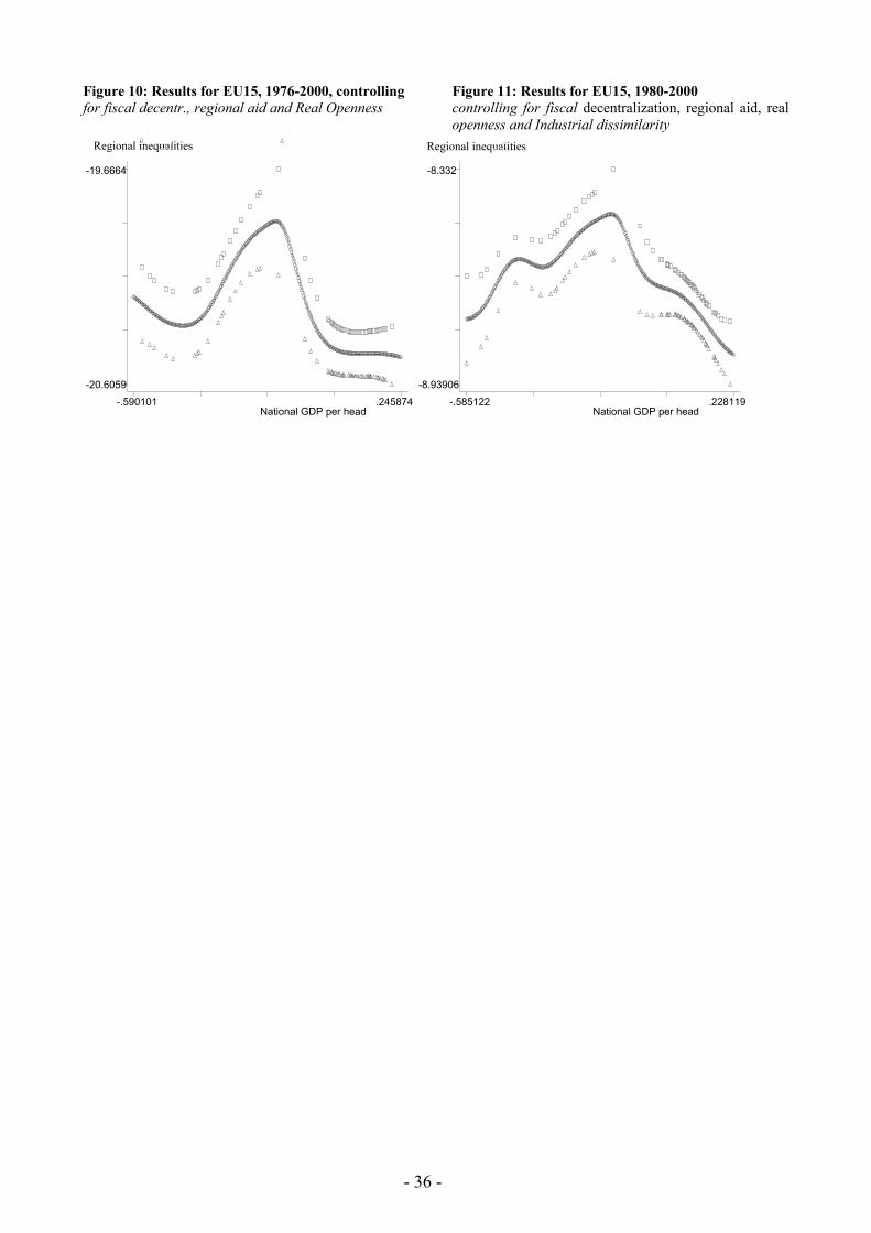
In Figures 8 through 11 we thus proceeded and re-estimated our semi-parametric
specification including these additional control variables in various combinations. The results
obtained in these figures must be compared to the one obtained previously in Figure 2 where we
included the national level of GDP per capita only as explanatory variable. Accordingly, regardless
of what fiscal decentralisation or openness variable we use, the estimated shape of the regional
inequality-national development link remains bell-shaped. In Figure 11 we also included our
dissimilarity index, although one must note that this meant reducing our sample period to start from
the 1980s. Nevertheless, one still observes the outlines of a bell-shaped curve.
- 25 -
5. Summary and conclusion
In this paper we examine the link between national economic development and regional
inequalities for a number of European countries and find strong evidence for a bell-shaped
relationship between these two variables. This evidence shows in particular that regional
inequalities inevitably rise as economic development proceeds but then tend to decline once a
certain level of national economic development is reached. Our results fit well with the original
predictions of Kuznets (1955) as well as with a model à la Tamura (1996) and Lucas (2000) where
the transition dynamics of regional economies towards their steady state level of income can
generate such a curve and where spillovers play a central role in transmitting growth and
technological progress across regions. Despite the fact that our results concern essentially the EU
experience, the pattern of regional development they describe provide a fairly general idea about the
relationship between national development and regional inequalities. Indeed, results including other
OECD countries tend to confirm the existence of such bell-shaped curve in regional development
for non-EU countries.
Our findings have also important policy implications for EU Cohesion policy. This policy is
aimed at boosting convergence and catching-up of lagging EU regions and at reducing regional
inequalities across the EU. The evidence presented here implies that some degree of regional
inequality is hardly avoidable, at least at the initial stages of development. The main reason for this
is that growth, because of its very nature, is unlikely to appear everywhere at the same time. It
follows that some degree of heterogeneity in regional economic development will necessarily
appear as countries are engaged into fast economic catching-up. This interpretation is further
reinforced by our results concerning European metropolitan areas. Cities are likely to play a major
role in fostering growth and technological diffusion. Our results tend to corroborate the fact that this
role is, however, likely to be more important for the relatively poor, rather than the relatively rich
EU countries. Our results thus suggest that regional policy and public investment should aim at
boosting national growth in order to guarantee greater national prosperity levels at the expense of
- 26 -
temporarily rising inequality, especially for the least developed countries such as the new EU
member states. In this sense, our results tend to support the findings of a recent paper by de la
Fuente (2004) who estimates that, in the case of Spain, which has largely benefiting from EU aid
since the late 1980ies, the allocation structural funds would have provided greater welfare through
more concentration on the most dynamic regions in order to favour nation-wide growth. As
suggested by de la Fuente (2004), the cost of re-shifting funds toward the most dynamic regions is
likely to be mitigated by national-level interpersonal income redistribution mechanisms. In our
analysis of the evolution of regional inequalities we try to take into account policy-related elements
such as Structural Funds and fiscal decentralisation variables which could possibly explain the
evolution of regional inequalities in the EU. However, other policy-related factors such as
countries’ own pro-active regional policy or redistribution mechanisms through social security
schemes might also influence the evolution of regional inequalities. A possible extension of this
work could be to consider these elements in order to analyse the efficiency of public policies
addressing regional disparities by taking explicitly into account the non-linearity inherent to the
evolution of regional inequalities evidenced in this paper.
- 27 -
References Alcalá, F. and A. Ciccone (2004), Trade and Productivity, Quarterly Journal of Economics 129(2), 613-646. Alonso, W. (1969), Urban and Regional Imbalances in Economic Developments, Economic Development and Cultural Change 17, 1-14. Barro, R.J. and X. Sala-i-Martin (2004), Economic Growth, 2nd Edition, MIT Press (Ed.). Beugelsdijk, M. and S.C.W. Eijffinger (2003), The Effectiveness of Structural Policy in the European Union: an empirical analysis for the EU15 during the period 1995-2001, CEPR discussion paper 3879. Blundell, R., Duncan, A., (1998). Kernel regression in empirical microeconomics, Journal of Human Resources 33 (1), 62–87. Boldrin, M. and F. Canova (2001). Europe’s regions: income disparities and regional policies, Economic Policy 16, 206-253. Bottazzi, L. and G. Peri, (2003), “Innovation and spillovers in regions: Evidence from European patent data”, European Economic Review 47(4), 687-710 Canova, F., (2004), “Testing for convergence clubs in income per capita: a predictive density approach”, International Economic Review 45(1), 49-77. Cheshire, P.C and D.G. Hay (1989), Urban problems in Western Europe. An Economic Analysis, Unwin Hyman, London. Ciccone, A. and Hall, R., (1996). Productivity and the density of economic activity. American Economic Review 86, 54-70. Ciccone, A., (2002). Agglomeration-effects in Europe, European Economic Review 46(2), 213-227. Clark, T. E. and van Wincoop, E. (2001). ‘Borders and business cycles’, Journal of International Economics 55, pp. 59–85. Coe, D. T. and E. Helpman, (1995), International R&D spillovers, European Economic Review, 39(5), 859-887. Davies, S. and M. Hallet, (2002). Interactions between National and Regional Development, HWWA Discussion Paper 207, Hamburg Institute of International Economics. Davoodi, H. and H. Zou, (1998), Fiscal decentralization and economic growth: a cross-country study, Journal of Urban Economics 43, 244-257. De la Fuente, A. and X. Vives, (1995). Infrastructure and Education as instruments of regional policy: evidence from Spain. Economic Policy 20, 13-51. De la Fuente, A. (2002) Does cohesion policy work? Some general considerations and evidence from Spain, IAE-CSIC Barcelona, mimeo.
- 28 -
De la Fuente, A. (2003), The effect of Structural Fund spending on the Spanish regions: an assessment of the 1994-99 Objective 1 CSF, FEDEA working paper 2003-11, Madrid. De la Fuente, A. (2004). Second-best Redistribution Through Public investment: A Characterization, an Empirical Test and an Application to the Case of Spain”, Regional Science and Urban Economics 34(5), 489-618. Durlauf, S.N. (2001), Manifesto for a growth econometrics, Journal of Econometrics 100, 65-69. Durlauf, S. N. and P.A. Johnson (1995), “Multiple regimes and cross-country growth behaviour”, Journal of Applied Econometrics 10(4), 365-84.” European Commission (2000), Real Convergence and Catching-up in the EU (ch. 5), In: The EU Economy Review, 2000 Review, Brussels. Frankel, J.A. and A. Rose (2002), “An Estimate of the Effect of Common Currencies on Trade and Income”, Quarterly Journal of Economics 117(2), 437-466. Fujita, M. and J.F. Thisse, (2002). Economics of Agglomeration. Cities, Industrial Location and Regional Growth. Cambridge University Press. Galor, O., (1996), “Convergence? Inferences from theoretical models”, Economic Journal 106(437), 1056-1069. Gianetti, M (2002), The effects of integration on regional disparities: Convergence, divergence or both? European Economic Review 46, 539-567. Härdle, W. (1990), “Applied non-parametric regression”, Econometric Society Monographs series 19, Cambridge University Press. Hirschman, A.O., (1958). The Strategy of Development, New Haven, CN : Yale University Press Head, K and Th. Mayer, (2000). “Non-Europe: The Magnitude and Causes of Market Fragmentation in the EU”, The Review of World Economics/Weltwirtschaftliches Archiv 136(2): 284-314. Iimi, A. (2005), Decentralization and economic growth revisited: an empirical note, Journal of Urban Economics, forthcoming. Jones; CH. I (2004), Growth and ideas, NBER working paper 10767. Kenen, P. B. (1969). ‘The theory of optimum currency areas: an eclectic view. In: Mundell R. and Swoboda A. K. (eds), Monetary Problems of the International Economy, University of Chicago Press, Chicago, IL, pp. 41–60. Kim, S. and R.A. Margo, (2003), Historical perspectives on U.S. economic geography, In: Handbook of Urban and Regional Economics, J.V. Henderson and J-F Thisse (eds). Kremer, M. (1993), “Population Growth and Technological Change: One Million B.C. to 1990”, Quarterly Journal of Economics 108: 681-716. Kuznets, S., (1955), Economic Growth and Income Inequality, American Economic Review 45(1), 1-28.
- 29 -
Li, Q. and Wang, S. (1998). A Simple Consistent Bootstrap Test for a Parametric Regression Function, Journal of Econometrics, 87, 145-165. Liu, Z. and T. Stengos, (1999), Non-linearities in Cross-country Growth Regressions: A semiparametric Approach, Journal of Applied Econometrics 14(5), 527-538. Lucas, R.E., (1988). “On the Mechanics of Economic Development”, Journal of Monetary Economics 22, 3-42. Lucas, R.E. (2000), “Some macroeconomics for the 21st Centrury”, Journal of Economic Perspectives 14 (1), 159-168. Organisation for Economic Cooperation and Development, (2004), Regions at work, OECD Economic Survey Euro area n°76, 153-248. Magrini, S. (1999), The evolution of income disparities among the regions of the European Union, Regional Science and Urban Economics 29(2), 257-281. Magrini, S. (2004): “Regional (Di)Convergence”, In: V. Henderson and J.-F. Thisse (eds.), Handbook of Urban and Regional Economics, Elsevier SciencePublishers, Amsterdam. Myrdal, G., (1957). Economic Theory and Underdeveloped Regions. London : Duckworth. Ottaviano, G.P. and J.F. Thisse (2003). Agglomeration and economic geography, In: Handbook of Urban and Regional Economics, J.V. Henderson and J-F Thisse (eds). Paap, R. and H. van Djik (1998), “Distribution and mobility of Wealth of Nationals”, European Economic Review 42, 1269-93. Parente, S.L. and E.C. Prescott, (1994), “Barriers to Technology Adoption and Development”, Journal of Political Economy 102(2), 298-321. Petrakos, G. and Saratsis, Y., (2000), Regional Inequalities in Greece. Papers in Regional Science 79(1), 57-74. Petrakos, G., A. Rodríguez-Pose and A. Rovolis, (2003). Growth, integration and regional inequality in Europe. Research papers in Environmental and Spatial Analysis 81, London School of Economics. Petrakos, G., G. Maier and G. Gorzelak (2000), Integration and Transition in Europe. The economic geography of interaction. Routledge Studies in the European Economy, New york. Pritchett, L., (1997), “Divergence, big time”, Journal of Economic Perspectives 11(3), 3-17. Quah, D., (1996a), “Empirics for Growth and Convergence”, European Economic Review 40, 1353-1375. Quah, D., (1996b), “Regional convergence clusters across Europe”, European Economic Review 40, 951-958. Quah, D., (1997), “Empirics for growth and distribution: stratification, polarization,and convergence clubs”, Journal of Economic Growth.2(1), 27-59.
- 30 -
Rodríguez-Pose, A. (1996) Growth and institutional change: The influence of the Spanish regionalisation process on economic performance. Environment and Planning C: Government and Policy, 14(1), 71-87. Rodríguez-Pose, A. and N. Gill, (2003). Is there a link between regional disparities and devolution? Research Papers in Environmental and Spatial Analysis 79, London School of Economics. Robinson, P., (1988), Root-N-consistent semiparametric regression. Econometrica 56: 931–954. Romer, P.M., (1990), “Endogenous Technological Change”, Journal of Political Economy 98: S71-S102. Solow, R.M. (1956), “A contribution to the theory of economic growth”, Quarterly Journal of Economics 106, 327-368. Stansel, D. (2005), “Local decentralization and local economic growth: A cross-sectional examination of US metropolitan areas”, Journal of Urban Economics 57, 55-72. Tamura, R., (1996), “From decay to growth: a demographic transition to economic growth”, Journal of Economic Dynamics and Control 20, 1237-1262. Temple, J., (1999), The New Growth Evidence, Journal of Economic Literature 37(1), 112-156. Wand, M.P., Jones, M.C., (1995). Kernel Smoothing. Chapman & Hall (eds.), London. Williamson, J., (1965), Regional inequality and the process of national development. Economic Development and Cultural Change 14, 3-45. Xie D., H. Zou, H. Davoodi (1999), Fiscal decentralization and economic growth in the United States, Journal of Urban Economics 45, 228-239.
- 31 -
Tables and Figures
Table 1: Level of national GDP and regional inequalities in Cohesion countries* GDP per capita Regional inequalities
Rest of the EU15 1.09 112 1.12 1.07 0.93 0.94 0.99 0.95
* Figures are relative to the EU15 countries, GDP per capita is measured at PPS Regional inequalities are measured using the standard deviation of the logarithm of regional GDP per capita qualities are measured using the standard deviation of the logarithm of regional GDP per capita, the figure for Portugal is for 1977. Values for country groups are in weighted (population) average Table 2: Summary Statistics for the EU15 countries, 1975-2000 GDP per capita Regional inequalities Mean Standard
Deviation Mean Standard
Deviation Austria 1.11 0.02 1.19 0.05 Belgium 1.11 0.03 1.18 0.05 Germany (Western only) 1.20 0.02 0.92 0.04 Spain 0.79 0.03 1.04 0.06 Finland 1.01 0.05 1.12 0.06 France 1.11 0.05 0.75 0.06 Greece 0.68 0.04 0.80 0.09 Italy 1.05 0.02 1.31 0.09 Netherlands* 1.11 0.04 1.01 0.09 Portugal** 0.64 0.07 1.17 0.20 Sweden 1.14 0.08 0.77 0.08 United Kingdom 1.04 0.02 0.75 0.03 Notes: Figures are comùputed relative to the EU25 average * Regional inequalities computed excluding Groningen region ** Regional inequalities computed excluding Alentejo region Table 3: Level of national GDP and regional inequalities in new Member States and candidate countries* GDP per capita (EU25=100) Regional inequalities 1995 2000 1995 2000 Average 0.43 0.45 1.10 1.22 Bulgaria 0.31 0.27 0.96 0.90 Czech Rep. 0.70 0.65 0.95 0.99 Estonia 0.34 0.42 1.52 1.54 Hungary 0.49 0.53 1.09 1.22 Lithuania 0.34 0.38 0.65 0.96 Latvia 0.30 0.35 1.46 2.21 Poland 0.41 0.46 1.43 1.35 Romania 0.30 0.25 0.83 1.06 Slovenia 0.68 0.73 0.60 0.58 Slovakia 0.44 0.48 1.53 1.38 * Figures are relative to the EU15 countries weighted average, weights given by population GDP per capita is measured at PPS and regional inequalities are measured using the standard deviation of the logarithm of the regional GDP per capita
- 32 -
Table 4: Parametric estimations, EU15 1975-2000 dependent variable : Standard deviation of regional regional GDP per capita (GDPc)
Real openness - - - 0.651*** 0.761*** (0.183) (0.186)
Dissimilarity - - - - -0.502 (0.467)
F-test country dummy 68.29 62.82 71.23 71.35 40.93 [P-value] [0.000] [0.000] [0.000] [0.000] [0.000] R2 0.76 0.77 0.77 0.78 0.77 # obs 310 287 287 287 240 Notes: (a) time dummies included; (b) standard errors in parentheses; (c) ***, ** and * indicate one, five and ten per cent significance levels respectively, all regressions include a constant term. Variables measured in terms of deviation from the sample average Figure1: Theoretical analysis of the relationship between National GDP per capita and regional inequalities.
.8
.6
log_std_dev .4
.2
0 4 6 8 10
National GDP per capita
- 33 -
Figures 2-11: Semi-parametric estimations results; X-axis: National GDP per capita, Y-axis: Standard deviation of regional GDP per capita (deviations with respect to EU average) The symbols □ and ∆ correspond to the optimal band points Figure 2: Results for EU15, 1975-2000 Figure 3: Results for EU15, 1975-2000 – using lagged
GDP values (2 and 5 –year lags)
Figure 4: Results for EU25, 1995-2000 Figure 5: Results for EU25, 1988-2000
inequality measures based on nuts2 regions only
Regional inequalities
National GDP per head
ver cu cl ver_2 Regional inequ ve
alitiesver_5r
4.3437 3.66107
2-year lag
no lag
5-year lag
-.585122 .981953 1.29326
.245874 .245874-.590101National GDP per head
Regional inequalities
National GDP per head
ve r cu cl cl Regional inequalities ver
cu
2.30034 2.92407
-1.17073 .689881 .773019
.486099 .309733-.882026National GDP per head
- 34 -
Figure 6: Results based on Functional Urban Areas Figure 7: Results based on OECD Territorial 1977-1996 Statistics, 1977-1996
Figure 8: Results for the EU15, 1976-2000, Figure 9: Results for EU15, 1976-2000, controlling for fiscal decentr., regional aid and openness controlling for fiscal decentr. in % of GDP,
regional aid and openness
Regional inequalities
National GDP per head
ver cu cl cl Regional ineq ties
ualcu iver
3.89684 4.38574
-.585122 .829799 .710118
-.969023.228119National GDP per head .468553
Regional inequalities ve cl
National GDP per head
r cu cl Regional inequalities cu
ver
-19.5194 -19.6133
-.590101 -20.4928 -20.5793
.245874National GDP per head .245874-.590101
- 35 -
Figure 10: Results for EU15, 1976-2000, controlling Figure 11: Results for EU15, 1980-2000 for fiscal decentr., regional aid and Real Openness controlling for fiscal decentralization, regional aid, real
openness and Industrial dissimilarity
Regional inequalities
National GDP per head
ver cu cl cl Regional inequalities
vercu
-19.6664 -8.332
-.590101 -20.6059 -8.93906
.245874National GDP per head .228119-.585122
- 36 -
Table A1: Number of regions and dataset used Country Eurostat/Cambridge
Econometrics database (NUTS2 regions)
Functional Urban Areas OECD Territorial Statistics
Australia - - 8 Austria 9 - 9 Belgium 11 4 3 Canada - - 12 Czech Republic 8 - 8 Denmark - - 3 Finland 5 - 6 France 22 22 23 Germany 31 (42*) 28 11 Greece 13 - 4 Hungary 7 - 7 Italy 21 17 20 Japan - - 10 Mexico - - 32 Netherlands 12 4 4 Norway - - 7 Poland 16 - 16 Portugal 7 - 7 Slovak Republic 4 - 4 Spain 18 16 18 Sweden 8 - 8 United Kingdom 37 24 - United States - - 51 Total # of observations 312** 180 72 * including new Landers ** 132 for EU25
- 37 -
- 38 -
Table A2: Statistical sources of explanatory variables used in Section 4.3* Indicator Definition Source Traditional Openness index (exporti,t+importi,t)/GDPi,t Ameco database, European
Commission, Directorate General for Economic and
Financial Affairs
Real openness index (exporti,t+importi,t)/GDPpi,t
where GDPpi,t is the GDP
expressed in purchasing power standard
Ameco database, European Commission, Directorate
General for Economic and Financial Affairs
Tradable openness index (exporti,t+importi,t)/GDPt
i,t where GDPt
i,t is the GDP of the tradable sectors
Ameco database, European Commission, Directorate
General for Economic and Financial Affairs
Industrial dissimilarity index
( ) ∑≠−=
iN
jkkkj
iiti K
NNK
,,, )15.0
1
where Ni is the number of regions located in country i and
∑ −=s
tkstjstkj xxK ,,,,,, 5.0
Where xs,j= share of sector s in total employment of region j
Cambridge Econometrics sectors s concern agriculture, construction, energy and manufacturing, market services and non-market services
Fiscal decentralization index Sum of local and regional total expenditures, excluding current and capital transfers to other levels of government, divided by the sum of local, regional and national expenditures, excluding intergovernmental transfers.
World Bank
Fiscal decentralization index (% of national GDP)
Sum of local and regional total expenditures, excluding current and capital transfers to other levels of government, divided by National GDP
World Bank
EU Regional aid Total EU payment for regional development from the European Regional development Fund (ERDF), the European Agricultural Guidance and Guarantee Fund (EAGGF), , and the European Social Fund (ESF) in % of national GDP
European Commission, Directorate General for Economic and Financial Affairs
* Indicators subscripts indicate country i and year t. Monetary variables are expressed in current euros