European Electricity Market

Model

András Mezősi

REKK

Sofia, 19.01.2017

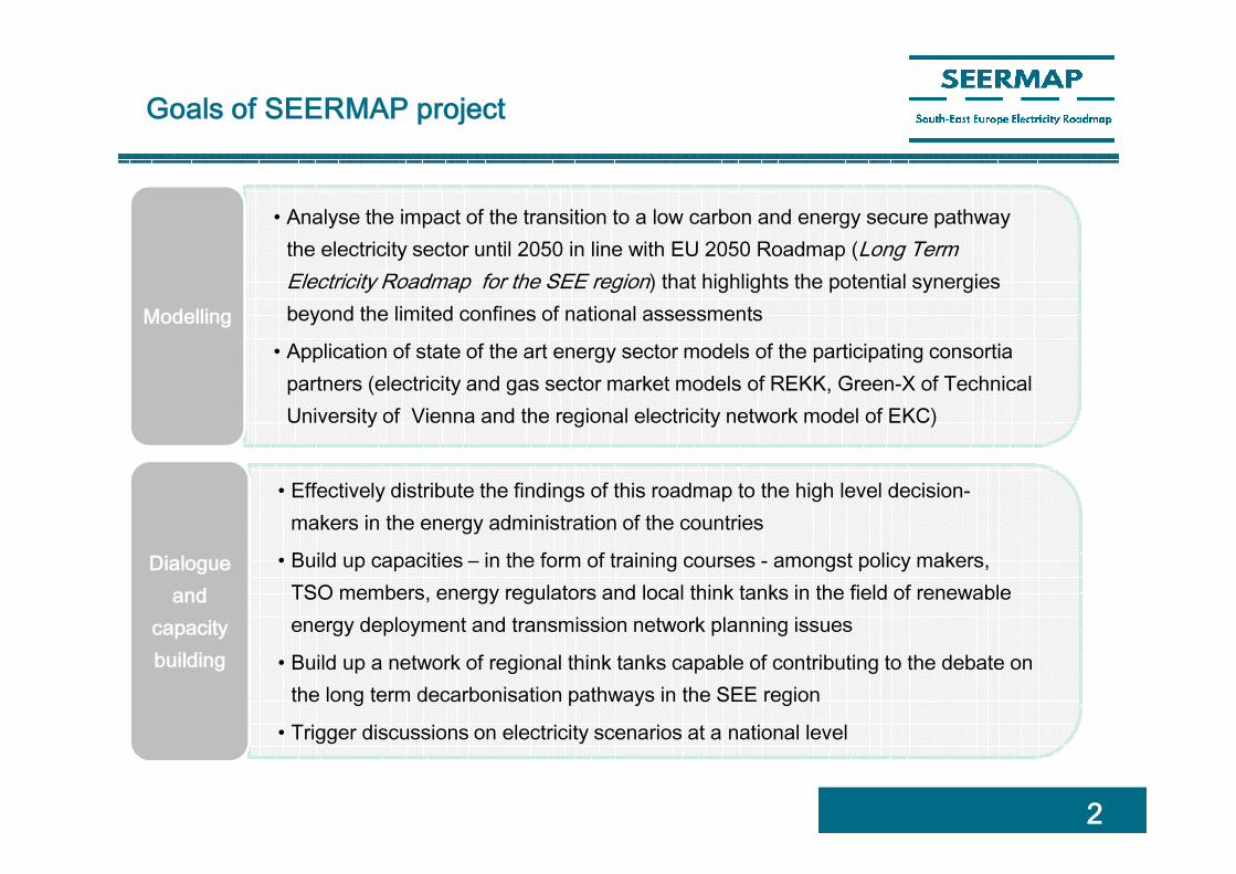
Goals of SEERMAP project

2

• Analyse the impact of the transition to a low carbon and energy secure pathway

the electricity sector until 2050 in line with EU 2050 Roadmap (Long Term

Electricity Roadmap for the SEE region) that highlights the potential synergies

beyond the limited confines of national assessments

• Application of state of the art energy sector models of the participating consortia

partners (electricity and gas sector market models of REKK, Green-X of Technical

University of Vienna and the regional electricity network model of EKC)

Modelling

• Effectively distribute the findings of this roadmap to the high level decision-

makers in the energy administration of the countries

• Build up capacities – in the form of training courses - amongst policy makers,

TSO members, energy regulators and local think tanks in the field of renewable

energy deployment and transmission network planning issues

• Build up a network of regional think tanks capable of contributing to the debate on

the long term decarbonisation pathways in the SEE region

• Trigger discussions on electricity scenarios at a national level

Dialogue

and

capacity

building

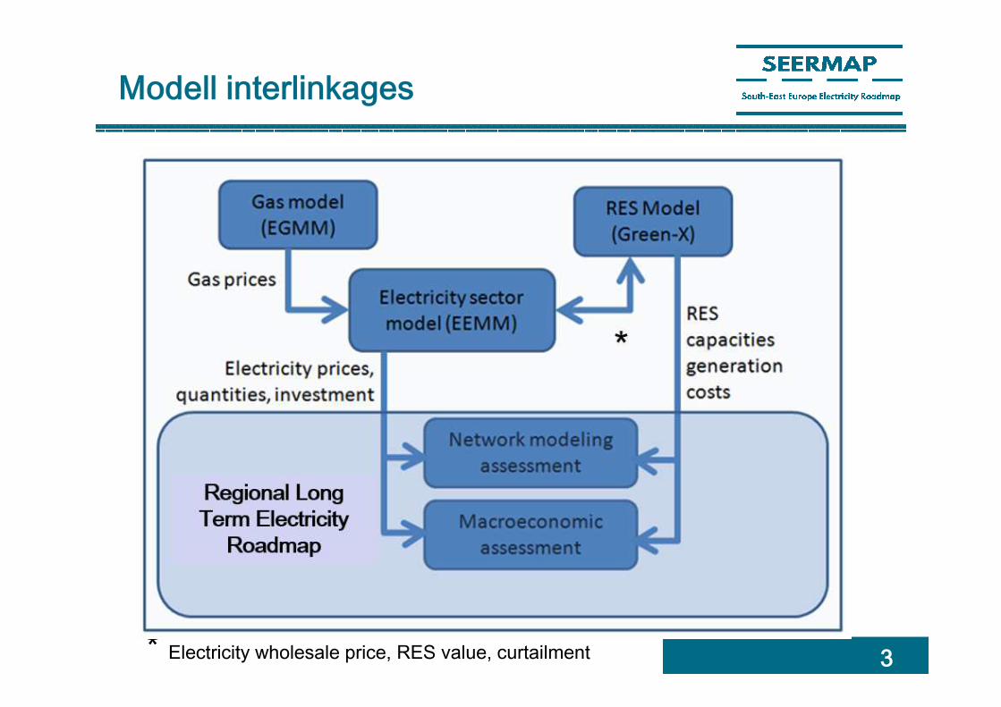
Modell interlinkages

* Electricity wholesale price, RES value, curtailment 3

4

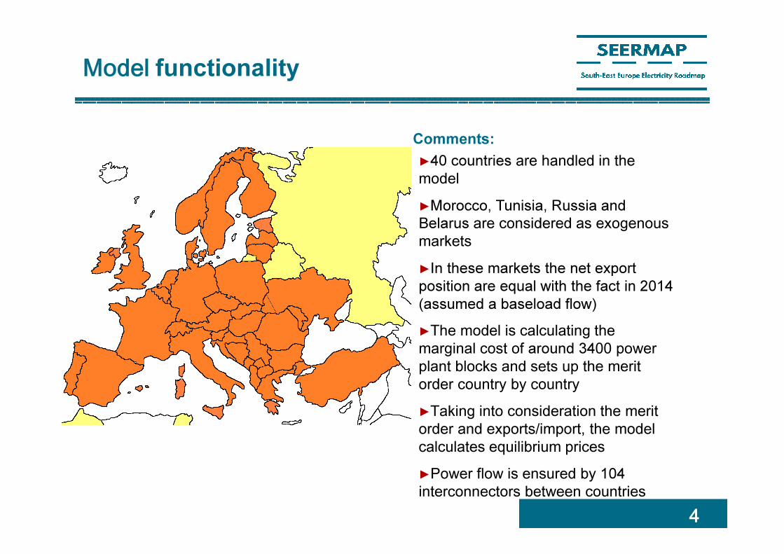
►40 countries are handled in the model

►Morocco, Tunisia, Russia and

Belarus are considered as exogenous markets

►In these markets the net export

position are equal with the fact in 2014

(assumed a baseload flow)

►The model is calculating the marginal cost of around 3400 power plant blocks and sets up the merit order country by country

►Taking into consideration the merit order and exports/import, the model calculates equilibrium prices

►Power flow is ensured by 104

interconnectors between countries

Comments:

Model functionality

5

Basic economics in the model

• Competitive behavior by power generators

‣ „if someone is willing to pay more for my energy than what it

costs me to produce it, then I will produce”

• Prices equalize supply and demand

• Efficient cross-border capacity auctions

‣ „we export electricity to wherever it is more expensive and import

from wherever it is cheaper”

• Capacity limits

‣ in production and cross-border trade

• Large country prices around the region are exogenous to

the model, the rest are determined by the model

6

Economic description and main

assumptions

►The applied model is a partial equilibrium

microeconomic model in which a homogeneous

product is traded in several neighboring markets.

►Production and trade are perfectly competitive,

there is no capacity withholding by market players.

►Production takes place in capacity-constrained

plants with marginal costs and no fixed cost.

►Electricity flows are modeled as bilateral

commercial arrangements between markets with a

special spatial structure.

►Power flows on an interconnector are limited by

NTC values in each direction.

►Fuel prices reflect power plant gate prices,

transportation/ transmission costs are taken into

consideration.

►Only ETS countries buy CO2 allowances

Main model assumptionsMain inputs and outputs of the model

►The model calculates regional power supply – demand balance at

certain capacity and import/export constraints

►Demand evolution, power plant capacities, availability and cross

border power flow defines market price

►Fuel prices are estimated based on available information

Marginal generation

cost

Available generation

capacity

Supply curves

by country

Cross-border

transmission

capacity

Demand curves

by country

Equilibrium prices

by country

Electricity trade between

countriesProduction by plant

Input

Outp

ut

Model

7

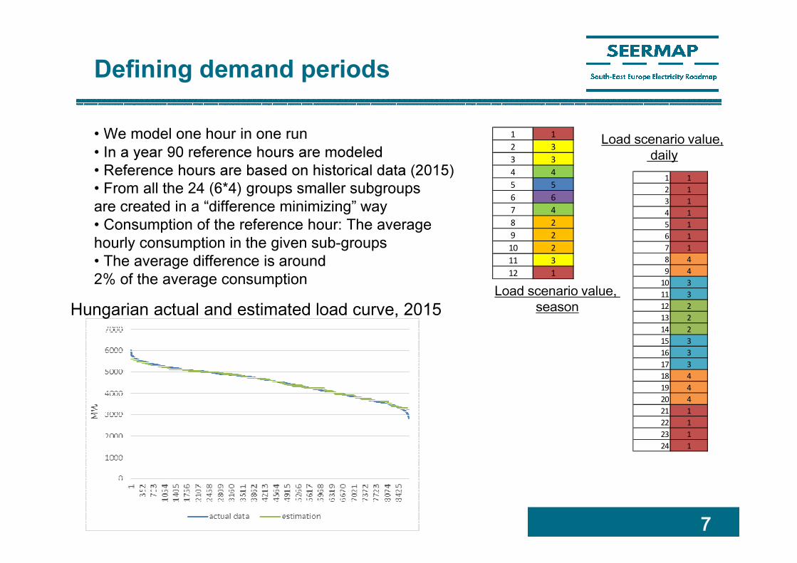
Defining demand periods

• We model one hour in one run• In a year 90 reference hours are modeled

• Reference hours are based on historical data (2015)

• From all the 24 (6*4) groups smaller subgroups are created in a “difference minimizing” way• Consumption of the reference hour: The average hourly consumption in the given sub-groups • The average difference is around 2% of the average consumption

1 1

2 3

3 3

4 4

5 5

6 6

7 4

8 2

9 2

10 2

11 3

12 1

Load scenario value,

season

1 1

2 1

3 1

4 1

5 1

6 1

7 1

8 4

9 4

10 3

11 3

12 2

13 2

14 2

15 3

16 3

17 3

18 4

19 4

20 4

21 1

22 1

23 1

24 1

Load scenario value,

daily

Hungarian actual and estimated load curve, 2015

8

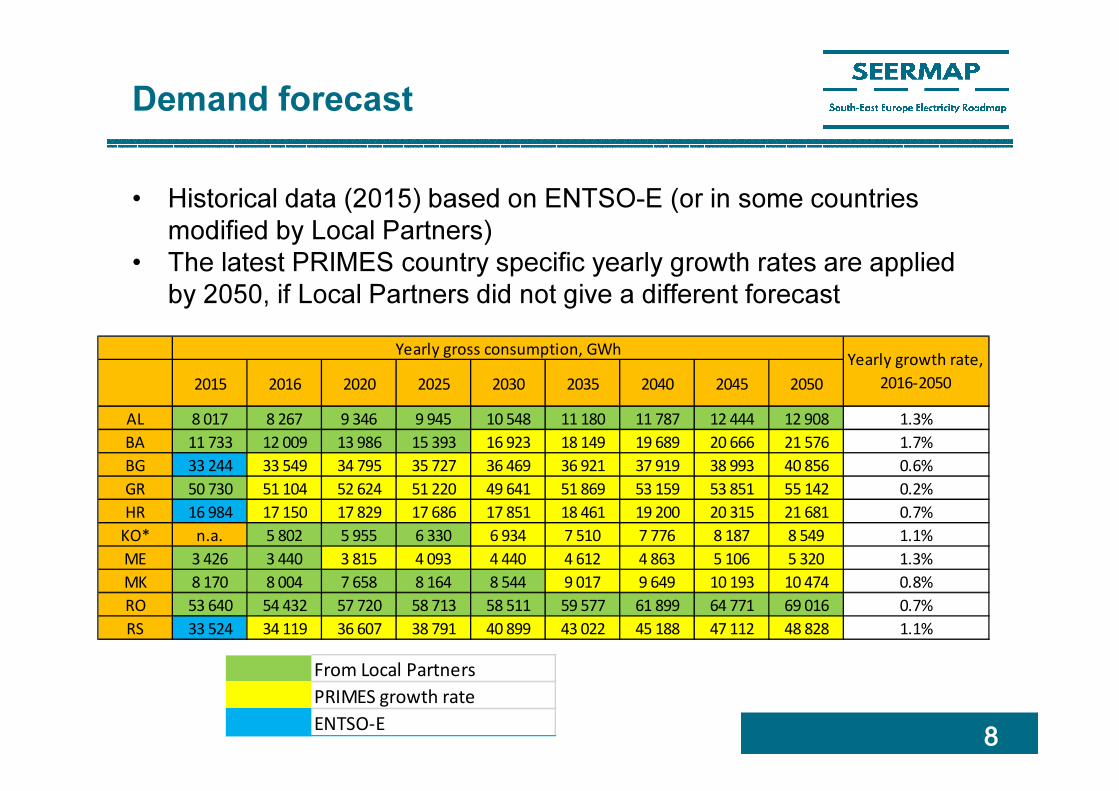
Demand forecast

• Historical data (2015) based on ENTSO-E (or in some countries

modified by Local Partners)

• The latest PRIMES country specific yearly growth rates are applied

by 2050, if Local Partners did not give a different forecast

2015 2016 2020 2025 2030 2035 2040 2045 2050

AL 8 017 8 267 9 346 9 945 10 548 11 180 11 787 12 444 12 908 1.3%

BA 11 733 12 009 13 986 15 393 16 923 18 149 19 689 20 666 21 576 1.7%

BG 33 244 33 549 34 795 35 727 36 469 36 921 37 919 38 993 40 856 0.6%

GR 50 730 51 104 52 624 51 220 49 641 51 869 53 159 53 851 55 142 0.2%

HR 16 984 17 150 17 829 17 686 17 851 18 461 19 200 20 315 21 681 0.7%

KO* n.a. 5 802 5 955 6 330 6 934 7 510 7 776 8 187 8 549 1.1%

ME 3 426 3 440 3 815 4 093 4 440 4 612 4 863 5 106 5 320 1.3%

MK 8 170 8 004 7 658 8 164 8 544 9 017 9 649 10 193 10 474 0.8%

RO 53 640 54 432 57 720 58 713 58 511 59 577 61 899 64 771 69 016 0.7%

RS 33 524 34 119 36 607 38 791 40 899 43 022 45 188 47 112 48 828 1.1%

Yearly gross consumption, GWhYearly growth rate,

2016-2050

From Local Partners

PRIMES growth rate

ENTSO-E

9

Components of marginal cost

Estimated heat

rate

Estimated self-

consumption

Fuel costCO2 emissions

costVariable OPEX

Marginal production

cost

Generation technologyFuel type and

price

EUA (CO2)

price

+ +

10

Power plants database

• Technology:

‣ Non-RES: Thermal, OCGT, CCGT, nuclear

‣ Renewable: Hydro (run-of-river, storage, pumped storage), wind, solar, tide and wave, geothermal

• Fuel type:

‣ Non-RES: coal, lignite, LFO, HFO, natural gas, nuclear

‣ Renewable: Hydro (run-of-river, storage, pumped storage), wind, solar, tide and wave, geothermal

• Existing power plant database

‣ Data sources

• National regulators

• System operators

• Individual power company and plant websites

• EWEA, EPIA

• PLATTS database

‣ All cross-checked with Eurostat and ENTSO-E aggregated value, all differences remained below 10%

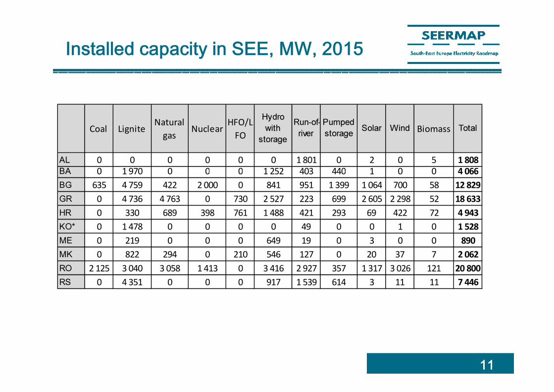
Installed capacity in SEE, MW, 2015

11

Coal LigniteNatural

gasNuclear

HFO/L

FO

Hydro

with

storage

Run-of-

river

Pumped

storageSolar Wind Biomass Total

AL 0 0 0 0 0 0 1 801 0 2 0 5 1 808

BA 0 1 970 0 0 0 1 252 403 440 1 0 0 4 066

BG 635 4 759 422 2 000 0 841 951 1 399 1 064 700 58 12 829

GR 0 4 736 4 763 0 730 2 527 223 699 2 605 2 298 52 18 633

HR 0 330 689 398 761 1 488 421 293 69 422 72 4 943

KO* 0 1 478 0 0 0 0 49 0 0 1 0 1 528

ME 0 219 0 0 0 649 19 0 3 0 0 890

MK 0 822 294 0 210 546 127 0 20 37 7 2 062

RO 2 125 3 040 3 058 1 413 0 3 416 2 927 357 1 317 3 026 121 20 800

RS 0 4 351 0 0 0 917 1 539 614 3 11 11 7 446

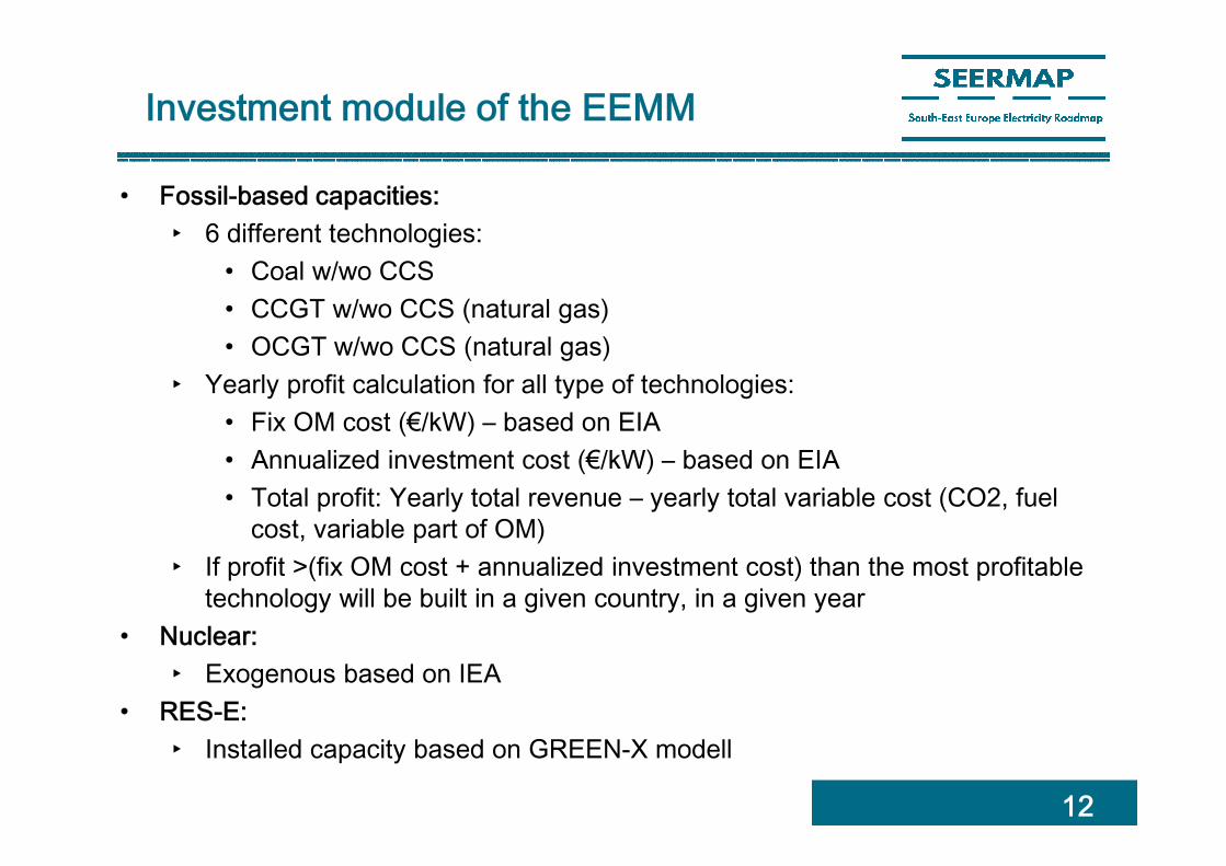
Investment module of the EEMM

• Fossil-based capacities:

‣ 6 different technologies:

• Coal w/wo CCS

• CCGT w/wo CCS (natural gas)

• OCGT w/wo CCS (natural gas)

‣ Yearly profit calculation for all type of technologies:

• Fix OM cost (€/kW) – based on EIA

• Annualized investment cost (€/kW) – based on EIA

• Total profit: Yearly total revenue – yearly total variable cost (CO2, fuel

cost, variable part of OM)

‣ If profit >(fix OM cost + annualized investment cost) than the most profitable

technology will be built in a given country, in a given year

• Nuclear:

‣ Exogenous based on IEA

• RES-E:

‣ Installed capacity based on GREEN-X modell

12

13

Efficiency parameters

• Taken from literature, dependent on the commission year and the

type of the PP

• Availability: Fossil: 95%; Geothermal: 85 %; Biomass: 80%; Tide and

wave: 85%

Year of

commissioningFuel efficiency and self-consumption for various power plant types

Gas/Oil ST Coal ST/Biomass CCGT

1960 37.0% 35.0% 50.0%

1965 38.0% 36.0% 50.0%

1970 39.0% 37.0% 50.0%

1975 40.0% 38.0% 50.0%

1980 41.0% 39.0% 50.0%

1985 42.0% 40.0% 50.0%

1990 43.0% 41.0% 50.0%

1995 44.0% 42.0% 52.5%

2000 45.0% 43.0% 55.0%

2005 46.0% 44.0% 56.5%

2010 47.0% 45.0% 57.0%

2015 48.0% 46.0% 58.0%

2020 49.0% 47.0% 59.0%

2025 50.0% 48.0% 60.0%

2030 51.0% 49.0% 61.0%

2035 52.0% 50.0% 62.0%

2040 53.0% 51.0% 63.0%

2045 54.0% 52.0% 64.0%

2050 55.0% 53.0% 65.0%

Self-consumption 5.0% 13.0% 5.0%

Availability of nuclear and RES-E

• Nuclear: Differ by country and season scenarios -> based on monthly historical data (ENTSO-E)

• Wind: Yearly utilization rate differ by country (source: IEA and calculated). Utilization depends on reference hour

• Solar: Yearly utilization rate differ by country (source: JRC and calculated). Utilization also depends on season and day scenarios

• Hydro:

– Run-of-river: Differ by season and country (based on historical data), baseload production within a day

– Storage: Differ by season and country (based on historical data), but the daily production is not baseload. High availability in peak hours, lower availability in off-peak hours

– Pumped storage: Historical utilization rates (Eurostat); produce in peak hours and consume in off-peak hours. Losses are also taken into account and differ by countries (based on actual data).

14

Special PPs - CHP

• CHP generators‣ Must-run power plants (production does not depend

on wholesale electricity price)

‣ Plant-by-plant determine whether is a CHP or not -> cross checked with aggregated database (Eurostat)

‣ Availability based on historical data

15

CHP

Season

1 2 3 4 5 6

Day

1 30% 6% 30% 3% 3% 0%

2 36% 6% 36% 3% 3% 0%

3 42% 6% 42% 3% 3% 0%

4 48% 6% 48% 3% 3% 0%

16

Fuel price forecasts

• Oil price

‣ Based on EIA Annual Energy Outlook (2016) and PRIMES (2016)

• Gas price

‣ Based on REKK EGMM (European Gas Market Model)

‣ Differ by country

• Coal

‣ Hard coal price equal ARA price and same in all countries

‣ Coal price forecasts are based on EIA: Annual Energy Outlook 2016

‣ Lignite price = hard coal * 0.55 (there is no liquid lignite market in

Europe)

• Nuclear

‣ Taken from literature, but irrelevant (never marginal)

• HFO, LFO

‣ Indexed to crude oil price

‣ Not especially important (hardly ever marginal)

Assumed fuel prices

17

Year 2016 2020 2025 2030 2035 2040 2045 2050

Crude oil; $2014/bbl

37.5 79.1 91.1 110.0 115.0 120.0 125.0 130.0

Exchange rate; $/€

1.1 1.1 1.1 1.1 1.1 1.1 1.1 1.1

CO2 price, €/t 4.2 15.0 21.5 31.5 35.0 52.0 80.0 87.0

ARA coalprice, €/GJ

1.5 2.0 1.9 1.9 2.0 2.0 2.0 2.0

18

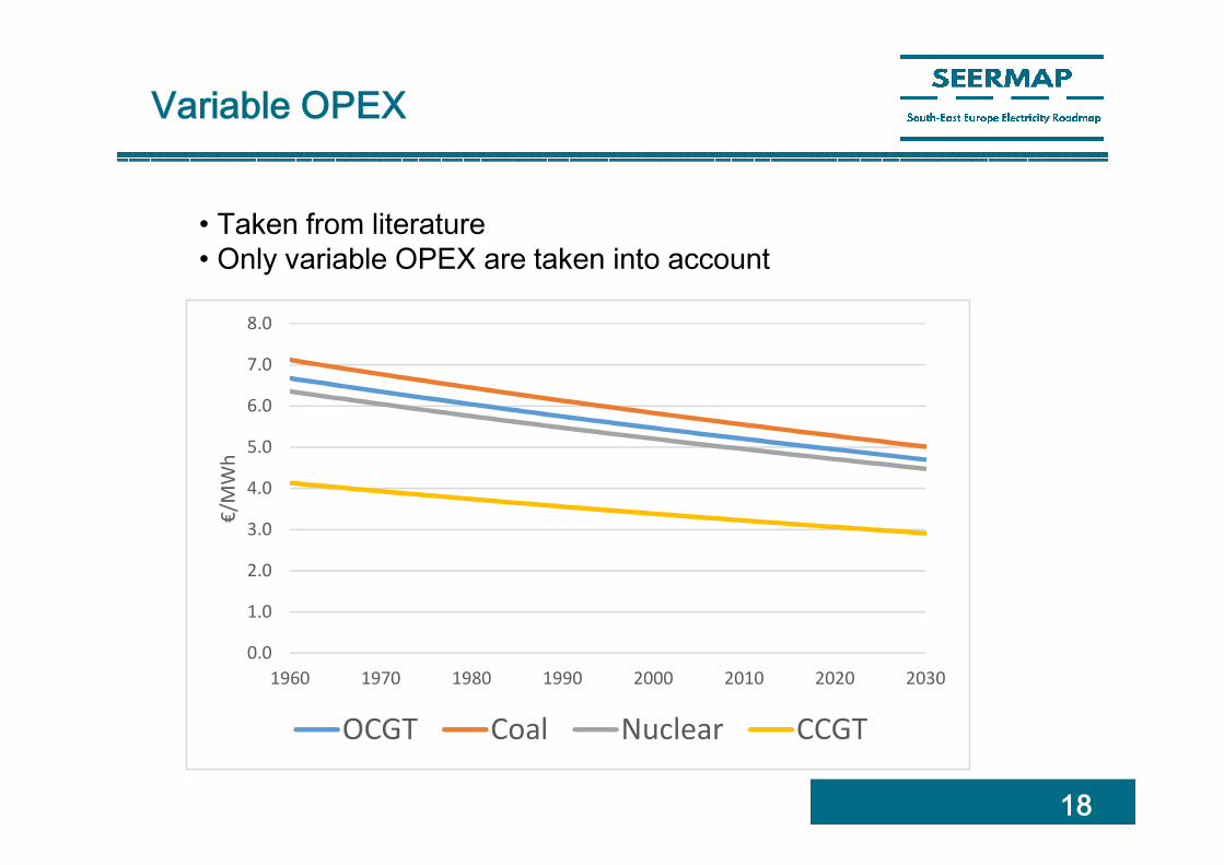
Variable OPEX

• Taken from literature

• Only variable OPEX are taken into account

0.0

1.0

2.0

3.0

4.0

5.0

6.0

7.0

8.0

1960 1970 1980 1990 2000 2010 2020 2030

€/M

Wh

OCGT Coal Nuclear CCGT

19

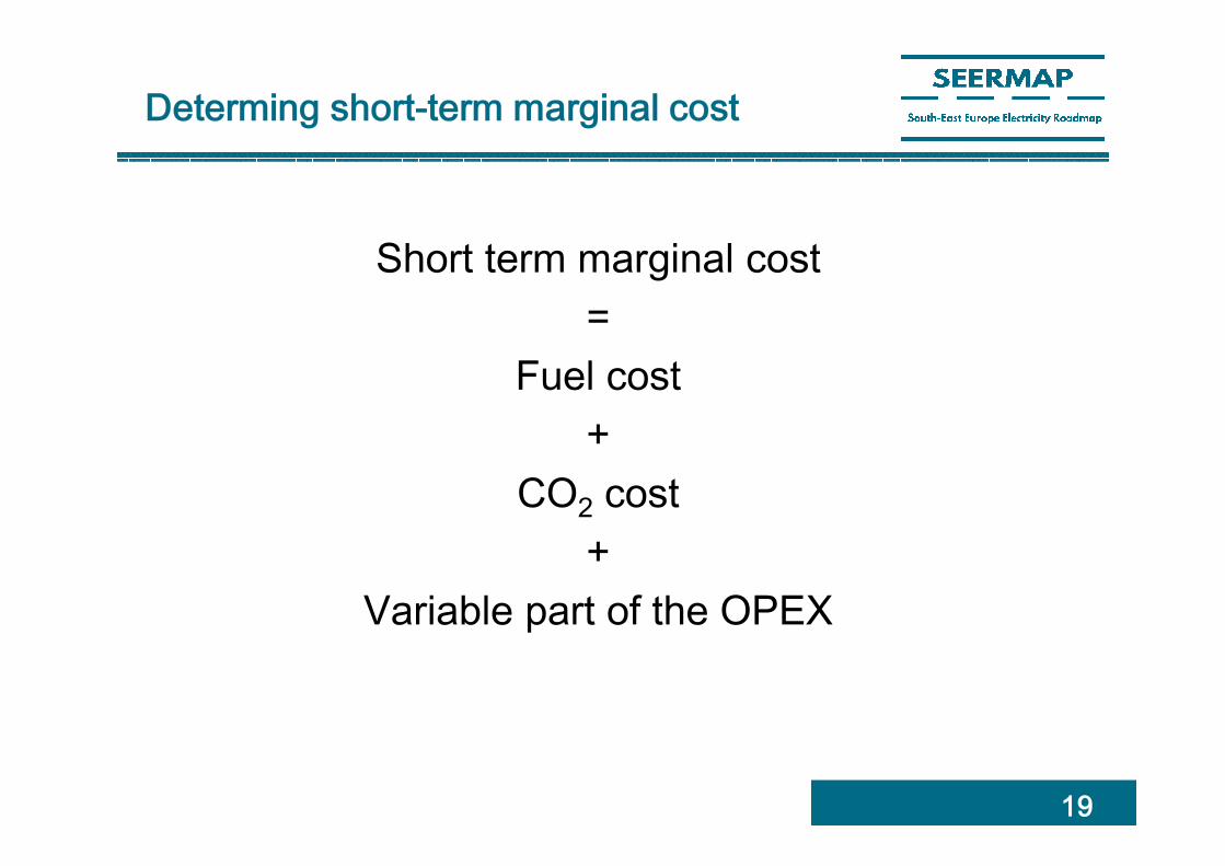
Determing short-term marginal cost

Short term marginal cost

=

Fuel cost

+

CO2

cost

+

Variable part of the OPEX

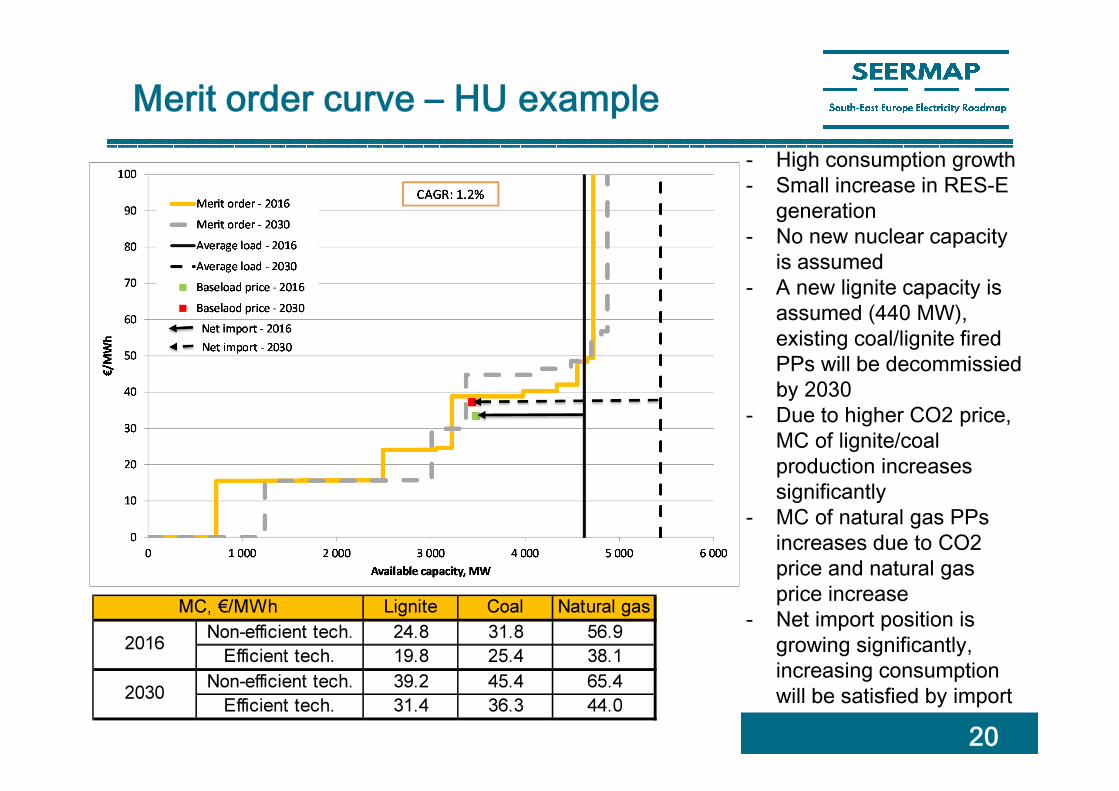
Merit order curve – HU example

20

- High consumption growth- Small increase in RES-E

generation- No new nuclear capacity

is assumed- A new lignite capacity is

assumed (440 MW), existing coal/lignite firedPPs will be decommissiedby 2030

- Due to higher CO2 price, MC of lignite/coal production increasessignificantly

- MC of natural gas PPsincreases due to CO2 price and natural gasprice increase

- Net import position is growing significantly, increasing consumptionwill be satisfied by import

Lignite Coal Natural gas

Non-efficient tech. 24.8 31.8 56.9

Efficient tech. 19.8 25.4 38.1

Non-efficient tech. 39.2 45.4 65.4

Efficient tech. 31.4 36.3 44.0

2016

2030

MC, €/MWh

Cross-border capacity

• One country -> one node (except DK and UA)

• NTC based trading

• NTC differ by borders, seasons and direction

• NTC value based on the historical value

published by ENTSO-E

• Future CBC expansions:

‣ based on ENTSO-E TYNDP 2014 and 2016

21

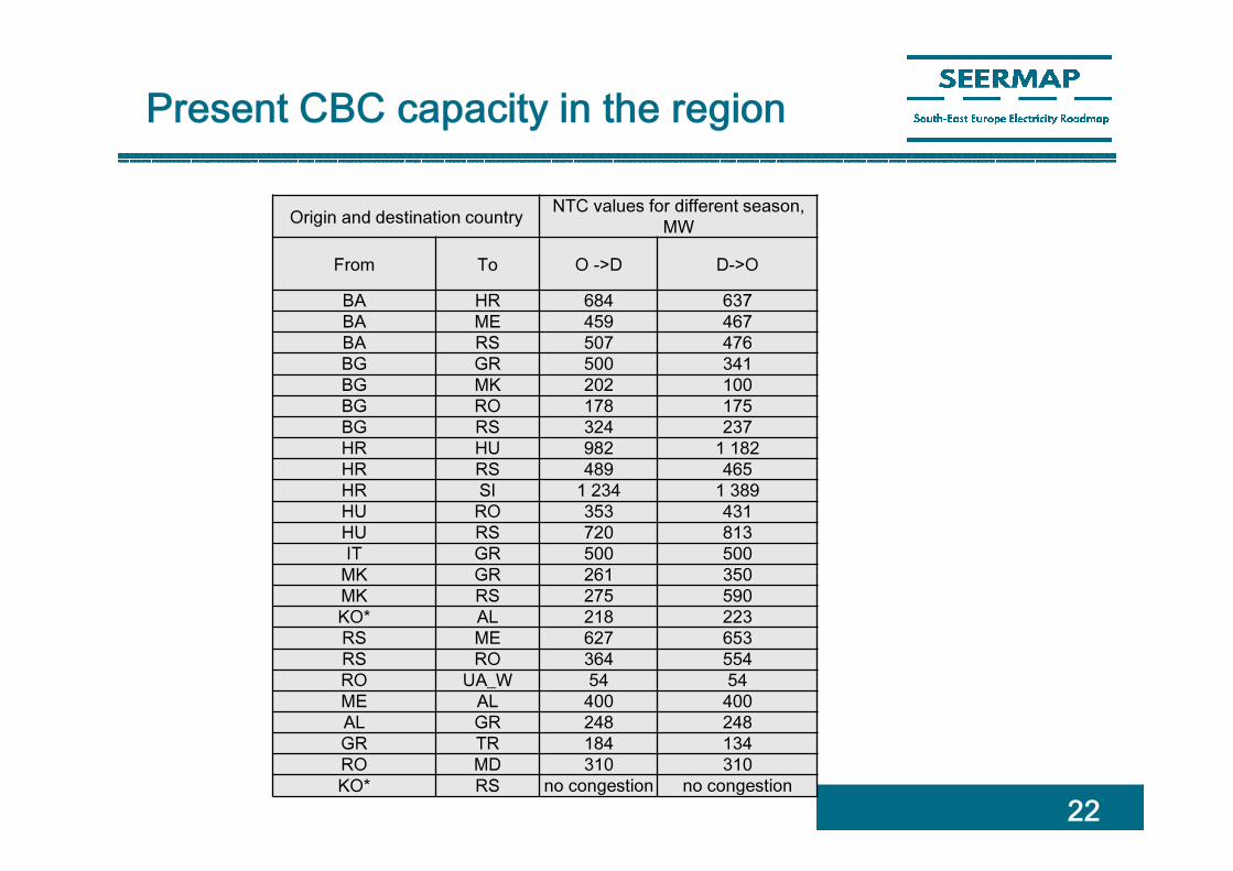
Present CBC capacity in the region

22

Origin and destination countryNTC values for different season,

MW

From To O ->D D->O

BA HR 684 637

BA ME 459 467

BA RS 507 476

BG GR 500 341

BG MK 202 100

BG RO 178 175

BG RS 324 237

HR HU 982 1 182

HR RS 489 465

HR SI 1 234 1 389

HU RO 353 431

HU RS 720 813

IT GR 500 500

MK GR 261 350

MK RS 275 590

KO* AL 218 223

RS ME 627 653

RS RO 364 554

RO UA_W 54 54

ME AL 400 400

AL GR 248 248

GR TR 184 134

RO MD 310 310

KO* RS no congestion no congestion

Future CBC development in the

region

23

New cross-border capacities

From ToYear of

commissioning

Investment

statusO -> D D -> O TYNDP 2016 code

ME IT 2019 1 1200 1200 28

BA HR 2022 3 650 950 136

BG RO 2020 2 1000 1200 138

GR BG 2021 2 0 650 142

RS RO 2023 2 500 950 144

ME RS 2025 2 400 600 146

KO* RS 2016 1 700 700 147a

AL MK 2020 2 250 250 147b

RS ME 2025 2 500 500 227a

RS BA 2025 2 600 500 227b

BA HR 2030 3 350 250 241

HR RS 2030 3 750 300 243

HU RO 2035 3 200 800 259

RS RO 2035 3 500 550 268

RS BG 2034 3 50 200 272

RS RO 2035 3 0 100 273

RS BG 2034 3 400 1500 277

GR BG 2030 3 250 450 279

IT GR 2033 4 1500 1500 E-Highway

IT GR 2037 4 1500 1500 E-Highway

IT GR 2043 4 1000 1000 E-Highway

IT GR 2046 4 1000 1000 E-Highway

UA_E RO 2038 4 700 700 E-Highway

The importance of cross-border capacities – an

effect of one-year delay of the commissioning of

the IT-ME undersea cable

24

- In REF IT-ME (1000

MW) will be

commissioned in 2018

- IT is a more expensive

country than the Balkan

region -> the new line

decreases the IT prices,

and increases the price

in the Balkan region

- This cable has a

significant effect on HU

baseload prices as well

25

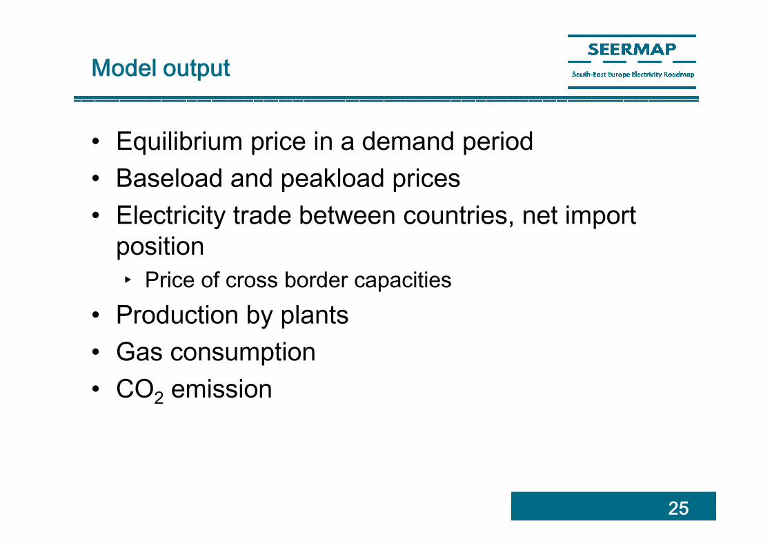
Model output

• Equilibrium price in a demand period

• Baseload and peakload prices

• Electricity trade between countries, net import

position

‣ Price of cross border capacities

• Production by plants

• Gas consumption

• CO2

emission

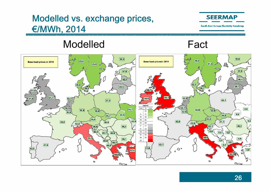
Modelled vs. exchange prices,

€/MWh, 2014

26

FactModelled

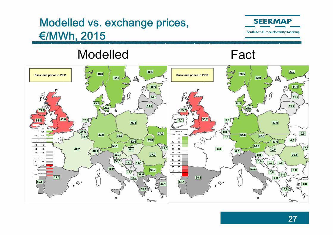
Modelled vs. exchange prices,

€/MWh, 2015

27

FactModelled

Relative differences of modelled vs. exchange

prices in the region, 2012-2015, %

28

-15%

-10%

-5%

0%

5%

10%

15%

AT CZ DE HU IT PL RO SI SK

Dif

fere

nce

(m

od

ell

ed

vs.

Fa

ct),

%

2012 2013 2014 2015

Thank you for your attention!