1

European Industrial Policy:

The Airbus Case

Damien Neven, University of Lausanne

Paul Seabright, University of Cambridge1

1 This paper reports the results of a simulation study commissioned by the UK Department of

Trade and Industry (EC/4878). Extracts from the Study are reproduced with the permission of

the DTI and the Controller of HMSO. We are grateful to the Air Division of DTI, and especially

to Michael Hodson and Robert Waters, for their detailed help and advice; to John Sutton for

comments on the report of the original study; to David Begg and Gene Grossman for comments

on the first draft of this paper; to Lars-Hendrik Roeller for comments and advice throughout the

project; and to Lisa Anderson for outstanding research assistance. The usual disclaimer applies

with particular force: the views reported in the paper are those of the authors alone, and not

those of any of the above individuals or institutions.

2

Abstract

This paper estimates the impact that Airbus’s presence has had on the market for large

commercial airliners. Our model reproduces (in a multi-stage) game a stylised characterisation

of six main stages in the development of the large commercial airliner market, allowing for

three players (Boeing, Airbus and McDonnell Douglas) and four market segments. The model

is then used to ask a number of counterfactual questions about what would have happened in a

variety of circumstances (notably ones in which Airbus did not enter the market). Besides

capacity and product developments, we also model the level of expenditures on research an

development in order to see whether Airbus’s presence has had an impact on the type and

technological specification of aircrafts produced. We find that given the prior presence of

McDonnell Douglas in this market, Airbus has had only a modest impact on the prices of

commercial airlines (an average of 3.5%). The reasons are twofold : first, although the Airbus

presence constraints the actions of Boeing, it weakens the incentive for McDonnell Douglas to

compete vigorously with Boeing. Secondly, by reducing Boeing’s market share, it prevents the

realisation of the substantial economies of scale and scope that are believed to exist in this

technology. Overall, this means that the consumer surplus argument for government subsidy to

Airbus is only weakly supported by the model. Consumer surplus benefits from a challenge to

Boeing have certainly been substantial but most of them could have been achieved by

McDonnell Douglas on its own. In terms of product development, we find that although

Airbus may have deterred McDonnell Douglas from producing an aircraft in the same category

of the A 300 (medium range, medium-bodied), it may in contrast have actually made it easier

3

for McDonnell Douglas to produce the MD-11 in competition with the A 330/340 and the

Boeing 777. This is because the loss of scale and scope economies by Boeing as a result of the

Airbus entry has substantially raised the cost to Boeing of producing the 777, making entry

more attractive for McDonnell Douglas even when Airbus’s presence is taken into account.

Finally, we find that the presence of Airbus reduces Boeing’s profits by at least $ 100 bn and

McDonnell Douglas’s by two-thirds. Airbus itself makes profits which are difficult to estimate

with confidence, but which may lie somewhere between $49bn and $52bn, of the order of a

billion dollars per annum and equivalent to a rate of return over the whole period of between

6% and 11%. If we give the same weight to profits and consumer surplus, this implies that

Airbus has had a large negative impact on world welfare but a comfortably positive impact on

European welfare.

4

1. Introduction

When should governments intervene to promote specific types of productive activity in

the economy? Answers to this question have been subject to periodic swings of fashion, but a

consensus has gradually emerged that intervention needs to be based on a sound account of

why unaided markets will fail to encourage adequately efficient levels of the activities

concerned, as well as a reasonable optimism that government failures will not lead to

distortions as significant as those market failures it is sought to correct. The application of this

consensus to actual cases, however, has generated substantial discord, particularly when the

activities under discussion are not public goods, but private goods which for one reason or

another are claimed to be supplied in inadequate quantity or quality. That the state should be a

vigilant referee of the competitive process is a view that would command widespread assent;

that it should be an active player in the competitive game is a much more debated and

debatable claim.

In no specific field of economic activity has the debate been more vigorous than in

commercial aerospace, where production has been supported and encouraged in covert or overt

ways by friendly governments around the world. Many reasons can be imagined for the

favoured status of aerospace, from the cynical ("politicians like shiny toys") to those more

firmly grounded in an analysis of market failure. There are persuasive grounds for thinking that

aerospace is likely to be subject to market failures, notably because of large scale economies in

5

production and the importance of research and development. Furthermore, these market

failures are often difficult for individual countries to overcome on their own, so aerospace has

given rise to significant international co-operation, the success or failure of which has

sometimes been seen as an important indicator of the prospects for co-operation in other fields.

The most celebrated instance of such cooperation is the European Airbus consortium,

which was formed in the late 1960s to challenge the dominance of the Boeing Corporation in

world markets; in 1994 for the first time, the former sold more commercial aircraft than the

latter. Its rivalry with Boeing and McDonnell-Douglas (MDD, also of the United States) has

led to fierce claims, in the GATT and other fora, about the role of public funding in generating

"unfair" competition.

The question what benefits flow from government support for commercial aerospace is

particularly pertinent to Airbus because the consortium owes its very existence to explicit

decisions by collaborating governments. Broadly speaking, three kinds of benefit have been

thought to flow from the Airbus presence in the market for large commercial jet airframes. The

first consists of lower prices to consumers resulting from a challenge to a dominant producer

(Boeing), benefits that could not be supposed to motivate a purely commercial competitor. The

second consists in various kinds of economic spillover from the advanced technology

embodied in the Airbus models; these might consist in the adaptability of technological

advances to other industries, or simply in the spur to technological improvement by Airbus's

own rivals. The third kind of benefit consists in whatever profits accrue to the consortium as a

result of its activities. However, such profits, if they exist, do not necessarily constitute a case

6

for government support, since profits are the reward for any normal unsubsidized commercial

activity.

Two kinds of argument have typically been advanced to show why governments may

be justified in subsidising activities that can be expected to be profitable. The first, which was

doubtless an important motivation for the original launch of the Airbus consortium, is a belief

that private capital markets often fail to fund activities that have a genuine expectation of being

profitable but happen to have a long investment horizon. This may be because private investors

are more averse to risk than governments ought to be, or because of institutional failures (such

as those due to internal agency problems) biasing decision-making towards projects with early

repayment profiles - for example, managers may inflate current profits at the expense of long-

term profits to persuade shareholders of their competence, and this may be rational even if

shareholders know they are doing so (Stein, 1989). Even if correct, such an argument also

requires confidence that government "short-termism" is a less serious problem, a confidence

that can falter in the face of such facts as the date of the British Government's announcement of

launch aid for the Airbus A-330/340 programme, just a few weeks before the general election

of 1987. The second argument, however, is more subtle, and appeals to the possibility that

certain activities may paradoxically be profitable (before subsidies) only because it is known

they enjoy government support. This is because the knowledge of government support may add

vital credibility to a producer's presence in the market, and may deter either predation by an

established rival or entry by a new one.

7

This idea that governments can affect the credibility and success of entry enjoyed

something of a vogue in the mid-1980s due to interest in so-called Strategic Trade Policy.

Governments will typically add to the credibility of entry by committing to absorb whatever

losses will occur and the provision of finance for fixed development cost (with repayment

linked to performance) will signal this intention. Such schemes have indeed been the most

important element of public support to the Airbus. Face with guaranteed entry, Airbus

competitors will presumably alter their competitive strategies (including pricing and product

developments). In particular, government support for the A-320 programme is often thought

to have induced Boeing to produce a new version of the 737 in the segment for narrow bodied,

small range aircrafts. In the absence of guaranteed competition, Boeing may have instead

opted for the development of a completely new aircraft in that market. Similarly, government

support for the A330/340 programme was thought likely not only to deter a very aggressive

response to Airbus from Boeing, but also perhaps to deter McDonnell-Douglas from

developing a long-range medium-bodied aircraft at all, especially given its highly visible

hesitation about whether to continue in the civil side of the aerospace business at all. In the

event, in spite of Airbus and its government support, McDonnell-Douglas went ahead with the

development of the MD-11, a model which is now in production.

Government can also affect the success of entry, if they do not affect the credibility of

the venture. By subsidizing production, government can affect the outcome of the competitive

game in such a way as to shift rents in favour of the domestic firms (see Brander and Spencer,

1985). As indicated above, public support to Airbus has taken mostly the form of a reduction

8

in fixed, development cost and has not affected variable production costs to an appreciable

extent. This aspect will thus be neglected in the present analysis.

This paper reports the results of a model whose purpose is to estimate the impact that

Airbus's presence has had on the market for large commercial airliners. In doing so we want to

ask what have been the costs and benefits of the decision to set up the consortium. This

exercise highlights the consequences of European public support to Airbus only to the extent

that in the absence of government support, the Airbus project would not have flown at all.

Indeed we do not model the way in which government support has added to the credibility of

the project and what would have happened without support (the Airbus project might have

survived, but in a very different form). The implicit assumption behind our policy conclusions

is therefore that government support has been decisive for the very existence of the project.

Besides addressing specific question about industrial policy in the airframe industry,

this paper also tries to draw some more general lessons about the appropriate conduct of

industrial policy by governments. Although it is only proper to be cautious about drawing

general lessons from a very particular case that has been analyzed according to an even more

particular model, the aerospace industry has been used in the past to make a number of general

claims about industrial policy2, and it is helpful at the very least to see whether we have learned

anything that casts light on these more general claims.

2 For example, Baldwin & Krugman argue that "for those who work on the "new" trade theory

that emphasize increasing returns, dynamics and imperfect competition, these economic

9

The model of the paper has a number of important features. First, it is a model of a

sequence of production decisions taken over a forty year period since the 1950s and affecting

output and sales over six decades. The aim has been to reproduce a stylized characterisation of

six main stages in the development of the large commercial airliner market (including a stage

that has not yet taken place, namely the development of replacements for the Boeing 747).

Then the model is used to ask a number of counterfactual questions about what would have

happened in a variety of circumstances (notably ones in which Airbus did not enter the

market). Secondly, we explicitly model (albeit in a highly simplified way) decisions about the

development of new models and the level of expenditure on research and development, in

order to see whether Airbus's presence has had an impact on the type and technological

specification of aircraft produced as well as on their quantity and price. Thirdly, the model is a

linear one, which means that it uses a simplified (and therefore tractable) approximation to

underlying technologies and market conditions that may be very far from linear. The reliability

of the approximation is higher for small changes around observed historical outcomes, but is

more suspect the more radical the counterfactual simulations that are run. Fourthly, reliable

data are available for only some of the parameters of the model; for others we have had to rely

on informed guesses, or calibrations that are consistent with observed history. Some of our

characteristics would in and of themselves make aircraft a natural target for study" (1988); and

that "the presence of dynamic factors....[makes the industry] a uniquely rewarding subject for a

trial run (of new trade theories and policies)" (1987).

10

simulation outcomes (those concerning outputs and, to a lesser extent, prices) are more robust

to uncertainties about these parameters than others (probably the least robust, unfortunately, are

our estimates of profits).

A number of striking conclusions nevertheless emerge from the simulations. First,

given the prior presence of McDonnell-Douglas in this market, Airbus has had only a modest

impact on the prices of commercial airliners (an average of 3.5%). The reasons are twofold:

first, although the Airbus presence constrains the actions of Boeing, it weakens the incentive

for MDD to compete vigorously with Boeing. Secondly, by reducing Boeing's market share it

prevents the realisation of the substantial economies of scale and scope (including learning

effects) that are believed to exist in this technology. Overall this means that the consumer

surplus argument for government subsidy to Airbus is only weakly supported by the model.

However, Airbus is nevertheless a more effective competitor to Boeing than is MDD, in the

sense that prices in a market with only Boeing and MDD would on average be 2% higher than

in a market with only Boeing and Airbus. This is principally because MDD produces aircraft

that have significantly higher running costs than those of Airbus. Furthermore, if MDD had not

been present in this market, a Boeing monopoly would have had dramatically higher prices (by

15% on average). So consumer surplus benefits from a challenge to Boeing have certainly been

substantial - but most of them could have been achieved by MDD on its own3.

3 Although MDD is a less effective competitor to Boeing than Airbus, it should not be thought

that under plausible alternative specifications of our model it might turn out to be a negligible

competitor to Boeing although still present in the market. This is because scale economies are

11

Secondly, the impact of Airbus on technological innovation by other producers has

been negative4. This is because Airbus entry has lowered their expected production runs and

thereby reduced the profitability of investment in fuel- and maintenance-efficiency. Aggregate

research and development in the industry has risen, but there has been greater duplication.

Thirdly, the Airbus presence reduces Boeing's profits by at least $100 bn. and MDD's

(which would anyway be low) by about two-thirds. Airbus itself makes profits which are

difficult to estimate with confidence, but which may lie somewhere between $40bn and $52bn,

of the order of a billion dollars per annum and equivalent to a rate of return over the whole

period of between 6% and 11%. If we give the same weight to profits and consumer surplus

this implies that Airbus has had a large negative impact on world social welfare but a

comfortably positive impact on European welfare.

so important in this technology that, if a producer enters the market at all, it will always do so at

a scale of production that makes a significant difference to its competitors' sales.

4 Airbus itself has of course contributed to technological progress via its own investments, but

the benefits of this should be fully reflected in the prices of its aircraft and consequently in its

profits. The externalities (which provide the rationale for public support) consist solely in the

impact on innovation by other producers. This model does not, however, measure pure

technological spillovers (such as any ability by Boeing to innovate more chaeply by copying

Airbus technology); it looks merely at the impact of competition on incentives to innovate.

12

Fourthly, the simulations shed an intriguing light on the rent-stealing argument.

Although the model does not enable us to model predation (since within each production stage

producers play a static game in production capacities), it does allow us to examine the impact

of guaranteed entry by Airbus on the entry decisions of other producers. Although Airbus may

have deterred MDD from producing aircraft in the same category as the A-300 (medium range,

medium-bodied), it may in contrast have actually made it easier for MDD to produce the MD-

11 in competition with the A330/340 and the Boeing 777. This is because the loss of scale and

scope economies by Boeing as a result of the Airbus entry has substantially raised the cost to

Boeing of producing the 777, making entry more attractive for MDD even when Airbus's

presence is taken into account.

This last point has potentially important implications in a wide range of contexts

outside the particular circumstances of commercial aerospace. In simple models of entry

deterrence it is often assumed that a firm faces symmetric rivals: actions that weaken or deter

one will weaken or deter them all. When a firm's rivals are significantly asymmetric, however,

this reasoning may be importantly flawed. Actions by firm A that weaken its rival firm B may

reduce the threat it poses to firm C by enough to more than offset any threat to firm C from

firm A. Interestingly, this phenomenon has important analogies in evolutionary biology, where

the introduction of predator species into an ecosystem has been shown in certain circumstances

13

to increase rather than reduce the number of other species the ecosystem can support5; in

recognition of these analogies we can even christen it the Starfish Effect.

It is important to note that the very circumstances which give rise to the Starfish Effect

- namely the presence of large economies of scale and scope - are precisely the circumstances

which have typically been thought propitious for the rent-stealing argument. For example,

Baldwin & Flam (1989) say that "the market for 30-40 seat commercial aircraft seems to be the

near ideal real world counterpart to the Brander-Spencer model [of rent-shifting]", because "the

industry is marked by very strong static as well as dynamic economies of scale; to enter

requires a large initial investment, and marginal costs are falling substantially due to learning

by doing. Policies that can affect capacity choices and output therefore have important effects

on costs and profits and on the distribution of profits and welfare between countries". The

model of this paper, however, suggests a more cautionary message: economies of scale and

5 Wilson (1993), p.164 reports an experiment by Robert Paine: "The starfish Pisaster

ochraceus is a key-stone predator of mollusks living in rock-bound tidal waters, including

mussels, limpets and chitons. It also attacks barnacles...Where the Pisaster strfish occurred in

Paine's study area, fifteen... of the mollusk and barnacle species coexisted. When Paine removed

the starfish by hand, the number of species declined to eight. What occurred was unexpected but

in hindsight logical. Free of the depredations of Pisaster, mussels and barnacles increased to

abnormally high densities and crowded out seven of the other species". See the discussion of

this and related phenomena in Sigmund (1993).

14

scope indeed increase the extent to which entry decisions can redistribute rents. But in the

presence of asymmetric rivals they also make it more likely that entry decisions of at least

some firms are strategic complements rather than strategic substitutes, and therefore make the

task of selective government intervention harder rather than easier.

Overall, the results of the model suggest that the external benefits from the entry of

Airbus into the market, though positive, have been modest. This suggests that government

support for the Airbus consortium will have been justified primarily if it proves to have been

profitable, and there is at least a reasonable chance that it will so prove.

2. The Market for Jet Airframes: a historical sketch

The commercial aircraft industry is characterised by unusually large static and dynamic scale

economies as well scope economies and it has been subject to significant demand and

technological shocks since the second world war.

To start with, development cost give rise to significant scale economies and these costs are

rising : development costs for the Boeing 777, which is now entering service, could be as

much as 4.3 (according to Tyson, 1992). On a cost per seat basis, development costs for this

aircraft have increased substantially relative to those incurred for the 747 in the early 70s.

With such initial outlays, fixed cost per unit are about halved when output is doubled from

an initial level of 200 units. Even at the scale of 500 units, a 50 % increase in output still

leads to a drop in average development costs of about 33 %. However large, fixed cost do

15

however play a relatively minor role by comparison with variable cost in generating scale

economies (for instance, at a production level of 500 units, average fixed cost do not

typically account for more 10 % of overall (fixed and variable average costs).

Indeed, most of the dynamics of costs is associated with variable costs (as much as 90 %

according to Klepper, 1990) ; the production of aircafts involves the coordination of

thousands of tasks and this process can be improved as experience accumulates. Such

learning by doing leads to important dynamic scale economies. The basic rule of thumb

used in the industry is that production costs decrease by 20% when output doubles (within

realistic production ranges).

Basic aircraft design can also sometimes be shared across a number of different models;

experience gained in production processes can also to some extent be applied to different

production lines. As a result, significant economies of scope can arise, and the more so, the

closer are the aircafts in terms of basic characteristics (fuselage size, wing span, type of

fitted engines). For instance, there is much commonality between the Airbus A330 and A

340. The Airbus A 330 is shorter than the A 340 but their fuselage has a common central

section and they share the same wings (except for engine pots - as the A430 has four engines

and A330 has only two). By contrast, the importance of scope economies between the A

330/340 family and the A320 (a much smaller aircraft) is much reduced. It is basically

associated with some avionics initially developed for the A320 which has been further

developed and adapted for the A330/340 family.

16

Overall, these costs characteristics are such that if the industry is analysed purely in terms of

static productive efficiency, it is at best a natural oligopoly (allowing for managerial

diseconomies), and possibly a natural monopoly (as claimed, for instance by Tyson, 1992).

According to Sutton (1995), the characteristics of technological improvements in this

industry provide a second additional reason behind high concentration. He suggests that

research and development on existing models is sometimes such that advanced versions can

effectively dominate particular segments. According to his analysis, a successful aircraft

design is therefore one that can be developed later in the lifetime of the aircraft into a

product that vertically dominates competitors. Such successful design experience two large

peaks in sales, one when the aircraft is launched and one when the advanced version comes

on sales. By contrast, unsuccessful design experience only one peak in sales (when it is

launched) and the market becomes eventually dominates by the successful design.

The first major development in the industry was triggered by the invention of the jet engine

and its application to civil aircraft. The first civil jet aircraft, the Comet (designed and

produced in Britain), flew in 1949 and entered service in 1952. Relative to previous piston

engines, jet engines allowed for much superior performance (in terms of speed and range)

but involved much larger fixed development costs. This change in cost structure inevitably

led to consolidation in an industry characterised by a larger number of independent

producers. The European industry was fragmented (including Hawker Siddely, Vickers, de

Havilland, Sud aviation, British Aircraft Corporation and Fokker) and its first mover, de

Havilland with the Comet, was grounded for several years because of technical problems.

In the meantime, both Douglas and Boeing developed their commercial aircrafts (the DC 8

17

and 707, respectively) and managed, because of a larger domestic market, to establish

themselves quickly and reap the necessary scale economies6. By the early sixties, the

European industry, victim of small national market and fragmented supply had all but

disappeared.

The basic design for the 707 and DC8 were soon developed to meet the diversified

domestic need of American airlines; first, the 727 was developed as a three engine version of

the 707, which could fly across the US. In order to meet the demand for short inter-city

links, Douglas produced the DC 9 by scaling down the DC8 and the 707 was further

reduced by Boeing, to produce the 737 (with two engines). This is the first important

product development in the industry, after the basic jet design were produced and it is

modelled as stage A in our simulation. Because of financial difficulties, Douglas also

merged with Mc Donnell (a company specialising in military procurement) at this time.

By the end of the 60s, the industry was affected by a new development in engine technology.

The turbo-fan technology, invented by Rolls-Royce, had the potential for much greater

thrust than the traditional turbo-jet technology. Such increase in power meant that much

larger aircraft could be flown and that the number of engines could be reduced for existing

6 Both the DC8 and 707 were derived from military projects (the (in)famous B47/B52 in the

case of Boeing) financed by the pentagon.

18

any aircraft sizes. This, in turn, could allow for significant savings in fuel7. The US

government then financed competing developments for a large scale transport aircraft by

Boeing and Mc Donnell Douglas and Lockheed. All three decided to develop commercial

applications. Mac Donnell Douglas and Lockheed designed tri-jets aircrafts (respectively

the DC 10 and the L1011 with similar range and capacity (350 passengers over 5 500

nautical miles). Boeing decided to leapfrog competition and designed a significantly larger

aeroplane (more than 400 passengers and more than 6000 nautical miles) with four engines.

This is the second major product development in the industry (modelled as stage B).

Lockheed eventually won the contract for the military transport aircraft and retreated from

the commercial market (after having incurred substantial losses).

By producing tri-jets with a capacity of 350 passengers, Lockheed and Mc Donnell Douglas

had however left what became known in the industry as a "hole in the sky". American

airlines wanted a 250 seat (wide body) aircraft that could fly across the US and save on fuel.

European airlines wanted an aircraft of similar size and range for some of their dense intra-

European routes. The Airbus first responded by designing the A300 and its derivatives the

A310, with an extended range and smaller capacity. Soon after, Boeing proposed the 757,

an extended version of the 737 as a stopgap measure8. However, as narrow body jet, the 757

7 In addition, turbo fans are much quieter than turbo jets as the core of the engine is

surrounded by a large flow of air.

8 According to industry analysts, the aircraft was designed to meet the particular needs of

British Airways in order to ensure that it would not defect to Airbus.

19

had insufficient capacity and could not be extended further. Boeing then developed the 767,

an entirely new design, which competed head on with the A300/A310. This is the third

major product development in the industry (modelled as stage C).

The deregulation of the American airlines industry and the development of air transport in

Europe gave rise to a new development; a short to medium range aircraft with a seating

capacity of about 150 was needed to support feeding into hubs in the US and to connect

capitals in Europe. Airbus moved first by developing the A320, fitted with many advanced

technological features like the fly by wire technology. This strategy was meant to

differentiate Airbus offering from that of Boeing and Mc Donnell Douglas, which both

developed new versions of existing aircrafts. Boeing developed the 737-300 (and later the

737-400) arguing that a much superior aircraft could soon be designed after new

developments in engine technology (the prop-fan) would materialise9. Mc Donnell Douglas

produced the MD 80, a derivative of the DC9. This is the fourth major product

development in the industry (stage D).

By the mid eighties, it became apparent that the DC 10 was becoming technologically

obsolete and that the 747 was used sometimes inefficiently. It was used on short term / high

density routes for which it had inadequate aerodynamic characteristics and long but

medium density flights (where the load factor was not inefficiently low). In addition, some

very long distances (Europe-Australia) could not be covered (at full load) without a stop-

9 Despite high intial hopes, this technology has been abandonned.

20

over. Airbus responded by producing the A330/A340 family. The A330 has two engines

and seats about 370 over 5000 miles, whereas the A340 has four engines and can cover more

than 7 000 miles (with a slightly reduced capacity). Boeing waited two years longer than

Airbus before designing a competing aircraft, the 777, which is somewhere in between the

A330 and A340. This delay may however prove crucial to the extent that the 777

incorporates the latest advances in engine technology such that it can come close the

performance of the A340 with only two engines. This stage of competition is currently

taking place and it is modelled as stage E.

Despite major improvements over the last twenty years, the 747 is now ageing and industry

analysts anticipate that the next major product introduction will occur in that segment.

Airbus is already talking about a potential A350 (600 seats ? ) and Boeing has unveiled plans

for a 800 seat aircraft (a double decker over the whole length of the aircraft). Is it unclear

however whether the market for such large aircrafts will materialise (see FT, April 3, 1995);

at this point, there are few interested airlines (British Airways and Singapore Airlines) but

much will depend on the development of airport facilities (restrictions to further airport

construction tend to favour mega aircrafts) and air traffic control (the safety distance

between large aircrafts is significantly shorter than that between small ones). This is the

last stage of competition in our model (stage F).

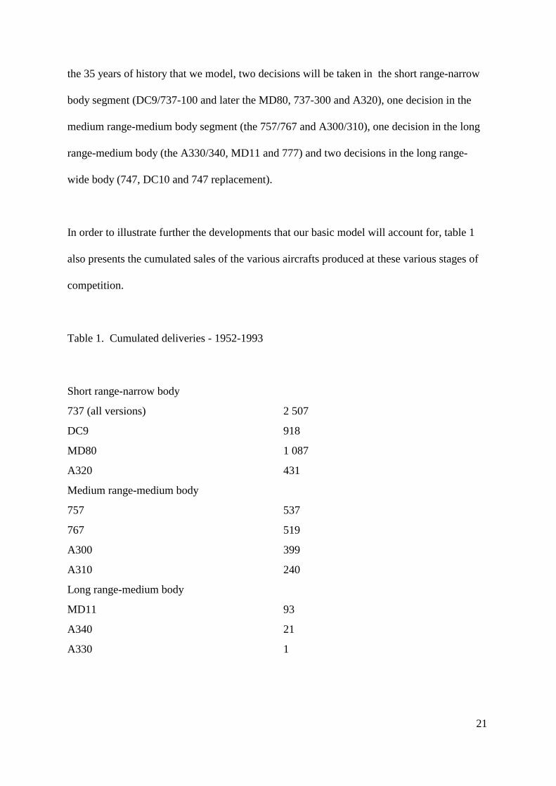
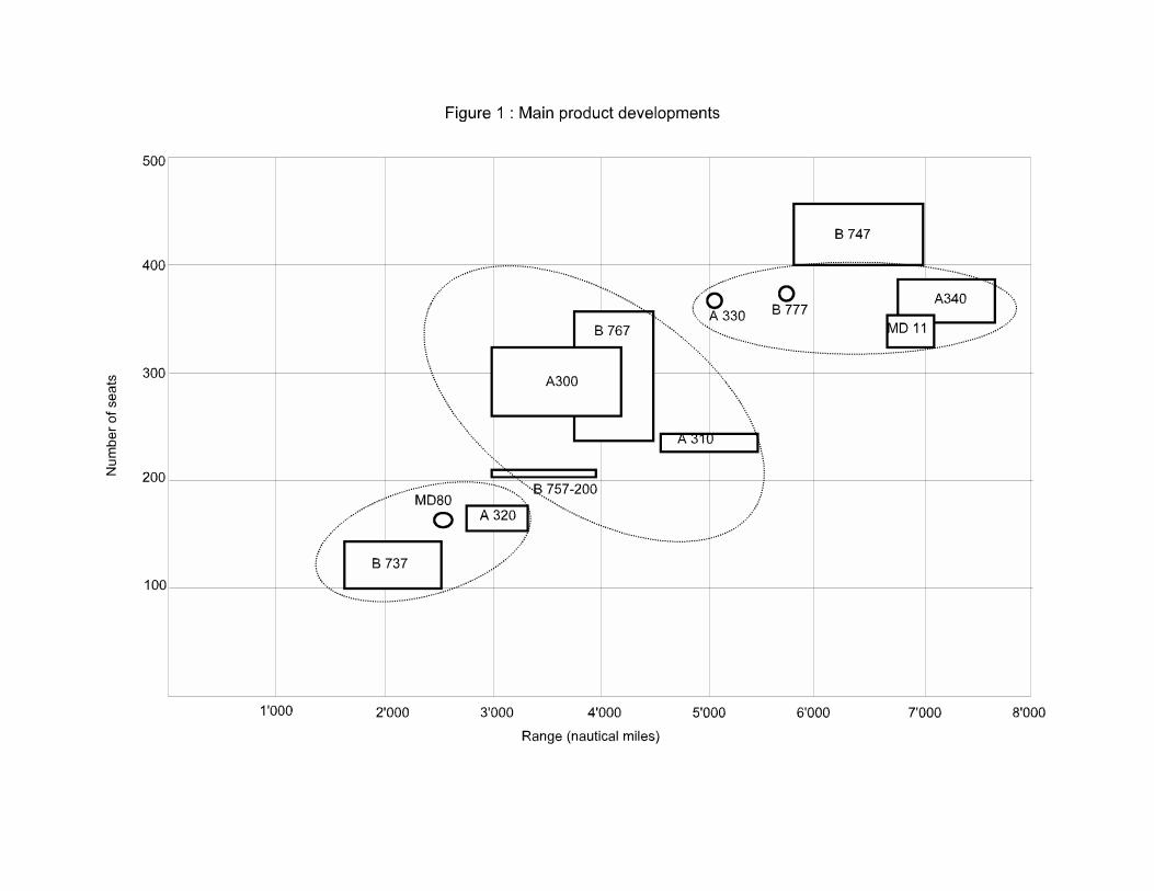
The main characteristics (in terms of range and single class seating) of the aircrafts produced

at these various stages of competition are presented in figure 1. The various market

segments associated with these product designed are also broadly presented; in the course of

21

the 35 years of history that we model, two decisions will be taken in the short range-narrow

body segment (DC9/737-100 and later the MD80, 737-300 and A320), one decision in the

medium range-medium body segment (the 757/767 and A300/310), one decision in the long

range-medium body (the A330/340, MD11 and 777) and two decisions in the long range-

wide body (747, DC10 and 747 replacement).

In order to illustrate further the developments that our basic model will account for, table 1

also presents the cumulated sales of the various aircrafts produced at these various stages of

competition.

Table 1. Cumulated deliveries - 1952-1993

Short range-narrow body

737 (all versions) 2 507

DC9 918

MD80 1 087

A320 431

Medium range-medium body

757 537

767 519

A300 399

A310 240

Long range-medium body

MD11 93

A340 21

A330 1

22

777 0

Long range-wide body

747 920

DC10 372

3. Previous studies of Airbus

Our model examines the impact of the entry of a third producer into the market for

large civilian passenger aircraft. Two items of previous research have modelled competition

purely as a duopoly between Boeing and Airbus. Both have claimed that the presence of Airbus

in this market has had overall negative consequences, both from the point of view of the world

as a whole and from the narrower point of view of European shareholders, consumers and

taxpayers. Baldwin & Krugman (1988) model competition in one market segment, between the

Airbus A300 and the Boeing 767. They estimate that the entry of Airbus resulted in substantial

consumer gains, but large losses of profits to Boeing and smaller but still substantial costs to

European taxpayers. The United States suffered as a whole from the policy, and Europe

suffered in aggregate for all but discount rates of 3% or less. The negative impact of Airbus

entry is due to the presence of substantial learning economies10 which are diluted by the

presence of competition.

10 By learning economies are meant reductions in marginal costs of production as production

runs increase.

23

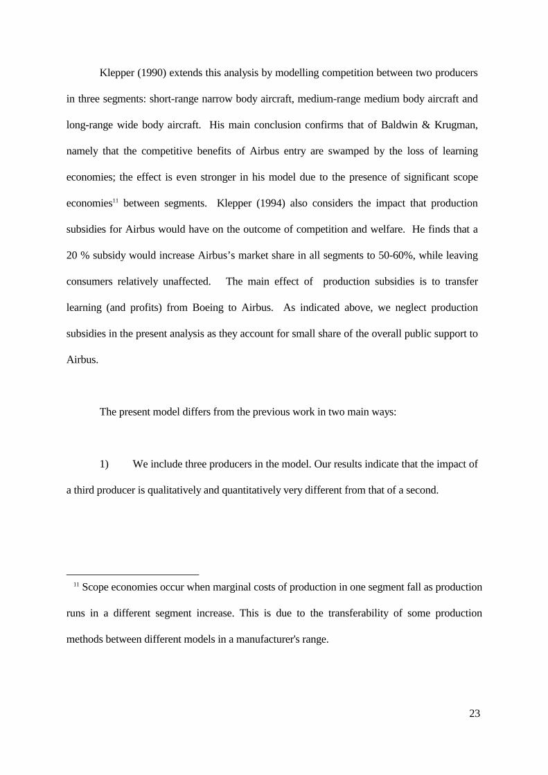
Klepper (1990) extends this analysis by modelling competition between two producers

in three segments: short-range narrow body aircraft, medium-range medium body aircraft and

long-range wide body aircraft. His main conclusion confirms that of Baldwin & Krugman,

namely that the competitive benefits of Airbus entry are swamped by the loss of learning

economies; the effect is even stronger in his model due to the presence of significant scope

economies11 between segments. Klepper (1994) also considers the impact that production

subsidies for Airbus would have on the outcome of competition and welfare. He finds that a

20 % subsidy would increase Airbus’s market share in all segments to 50-60%, while leaving

consumers relatively unaffected. The main effect of production subsidies is to transfer

learning (and profits) from Boeing to Airbus. As indicated above, we neglect production

subsidies in the present analysis as they account for small share of the overall public support to

Airbus.

The present model differs from the previous work in two main ways:

1) We include three producers in the model. Our results indicate that the impact of

a third producer is qualitatively and quantitatively very different from that of a second.

11 Scope economies occur when marginal costs of production in one segment fall as production

runs in a different segment increase. This is due to the transferability of some production

methods between different models in a manufacturer's range.

24

2) We model the decision to develop new products rather than treating

manufacturers' product ranges as given. This enables us to ask whether Airbus entry had an

effect on its rivals' product range and quality as well as on the prices and output of given

products. In addition we divide the market into four main segments.

The price of complicating the model in this way has been our adoption of a linear

specification for demand and production technology, as well as the assumption that producers

act as Cournot competitors (taking each others' capacity as given); together these

simplifications enable analytical solutions to be found to the game between producers at each

stage.

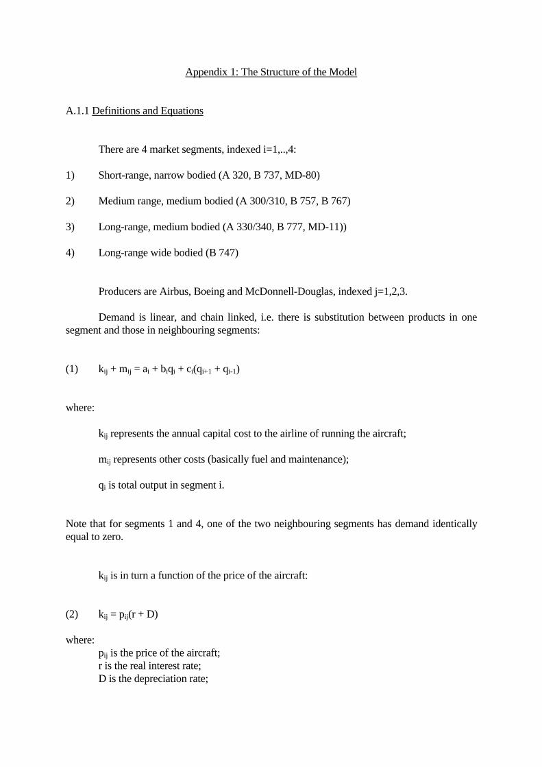
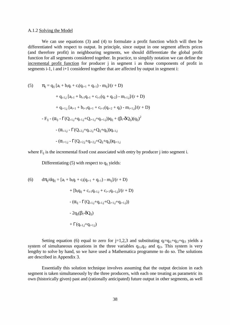
4. The model: a brief description

Our model (details of which are given in Appendix 1) describes a stylised history of the

market for large passenger aircraft since the 1960s as a sequence of six stages in the

development of four market segments. These four segments are:

1) Short-range, narrow bodied (SRNB)

2) Medium range, medium bodied (MRMB)

3) Long-range, medium bodied (LRMB)

4) Long-range wide bodied (LRWB)

25

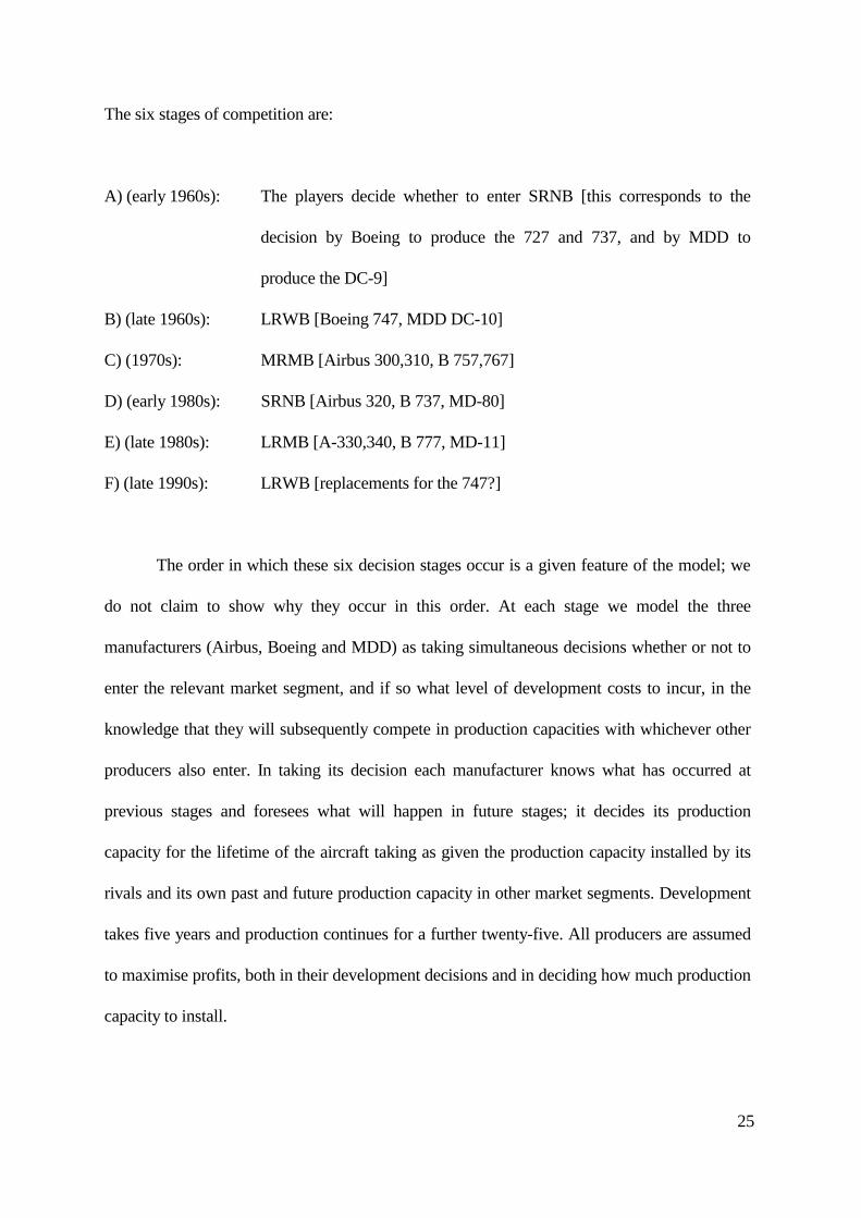
The six stages of competition are:

A) (early 1960s): The players decide whether to enter SRNB [this corresponds to the

decision by Boeing to produce the 727 and 737, and by MDD to

produce the DC-9]

B) (late 1960s): LRWB [Boeing 747, MDD DC-10]

C) (1970s): MRMB [Airbus 300,310, B 757,767]

D) (early 1980s): SRNB [Airbus 320, B 737, MD-80]

E) (late 1980s): LRMB [A-330,340, B 777, MD-11]

F) (late 1990s): LRWB [replacements for the 747?]

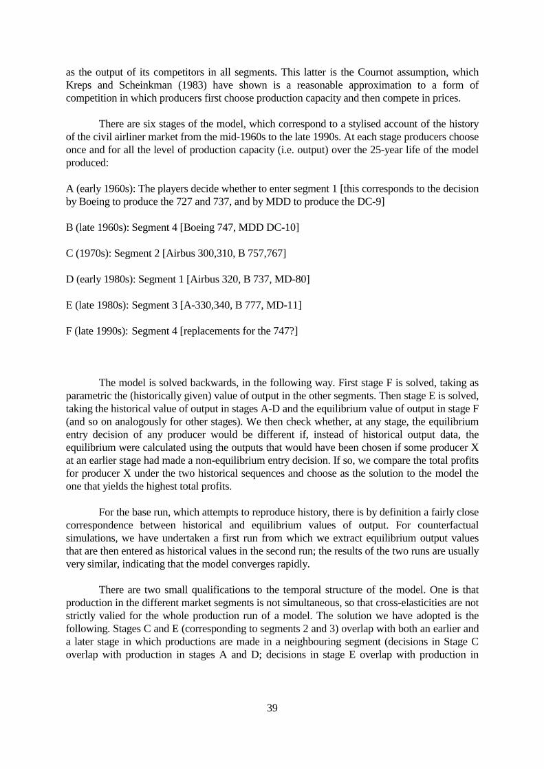
The order in which these six decision stages occur is a given feature of the model; we

do not claim to show why they occur in this order. At each stage we model the three

manufacturers (Airbus, Boeing and MDD) as taking simultaneous decisions whether or not to

enter the relevant market segment, and if so what level of development costs to incur, in the

knowledge that they will subsequently compete in production capacities with whichever other

producers also enter. In taking its decision each manufacturer knows what has occurred at

previous stages and foresees what will happen in future stages; it decides its production

capacity for the lifetime of the aircraft taking as given the production capacity installed by its

rivals and its own past and future production capacity in other market segments. Development

takes five years and production continues for a further twenty-five. All producers are assumed

to maximise profits, both in their development decisions and in deciding how much production

capacity to install.

26

These assumptions about taking capacity as fixed require further comment. They fall

into three categories. First, there is the assumption that a single producer's capacity, once

installed, cannot be changed. This is clearly very unrealistic when we consider that production

in practice continues for 20-25 years for most aircraft models. It may, however, be an adequate

approximation to a more realistic situation in which changing production capacity is

sufficiently expensive to outweigh any likely strategic advantage of changing it once it has

been installed. A producer will not wish to make a unilateral change in installed capacity unless

this would induce some favourable reaction from a competitor (otherwise this level of capacity

would not have been optimal in the first place); our assumption implies that the prospects of

any such reaction are not great enough to outweigh the costs of a change. We have made this

assumption because to do otherwise would greatly complicate the model, which in its six-stage

form is already complicated enough at least for our taste. However, one extension seems to us

potentially well worth exploring, though we cannot do so in this paper. This would be to take

seriously the idea that aircraft sales at a given production stage typically follow a twin-peaked

pattern. One way to model this would be to suppose that capacity can be changed half-way

through a production run, and an aircraft's technical specifications can be upgraded, in response

to new information that has been revealed about market conditions. To model this would

involve, in addition to a doubling of the number of decisions about production capacity, a

satisfactory modelling of uncertainty and its resolution.

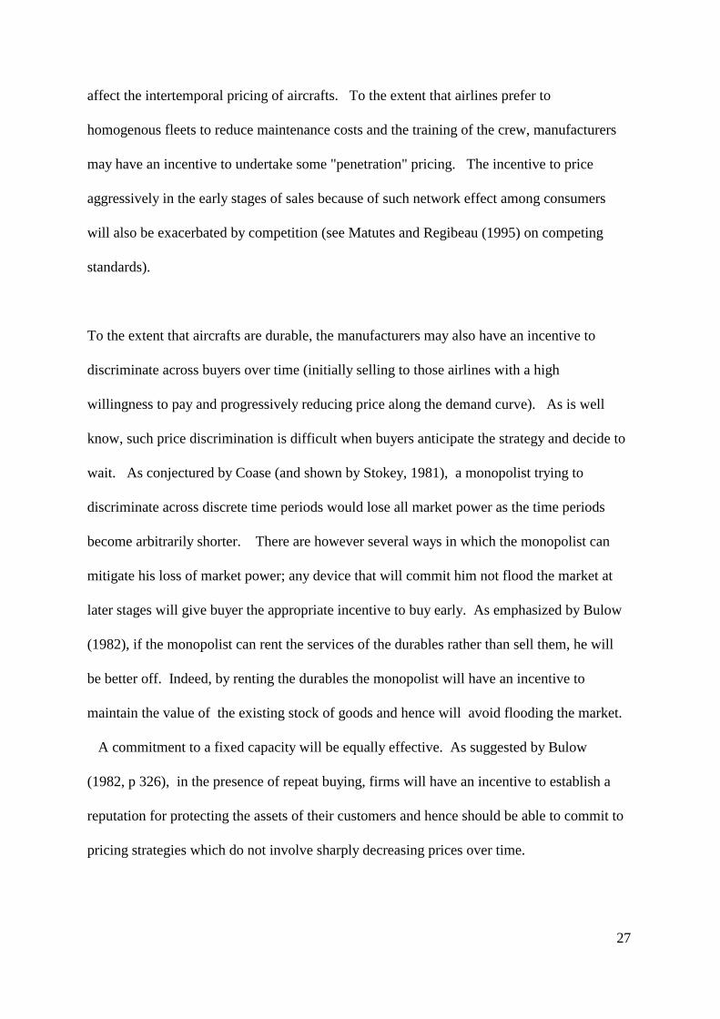
The second assumption worth commenting upon is the assumption that intertemporal

pricing issues (within segments) can be ignored. A number of different constraints will

27

affect the intertemporal pricing of aircrafts. To the extent that airlines prefer to

homogenous fleets to reduce maintenance costs and the training of the crew, manufacturers

may have an incentive to undertake some "penetration" pricing. The incentive to price

aggressively in the early stages of sales because of such network effect among consumers

will also be exacerbated by competition (see Matutes and Regibeau (1995) on competing

standards).

To the extent that aircrafts are durable, the manufacturers may also have an incentive to

discriminate across buyers over time (initially selling to those airlines with a high

willingness to pay and progressively reducing price along the demand curve). As is well

know, such price discrimination is difficult when buyers anticipate the strategy and decide to

wait. As conjectured by Coase (and shown by Stokey, 1981), a monopolist trying to

discriminate across discrete time periods would lose all market power as the time periods

become arbitrarily shorter. There are however several ways in which the monopolist can

mitigate his loss of market power; any device that will commit him not flood the market at

later stages will give buyer the appropriate incentive to buy early. As emphasized by Bulow

(1982), if the monopolist can rent the services of the durables rather than sell them, he will

be better off. Indeed, by renting the durables the monopolist will have an incentive to

maintain the value of the existing stock of goods and hence will avoid flooding the market.

A commitment to a fixed capacity will be equally effective. As suggested by Bulow

(1982, p 326), in the presence of repeat buying, firms will have an incentive to establish a

reputation for protecting the assets of their customers and hence should be able to commit to

pricing strategies which do not involve sharply decreasing prices over time.

28

These various commitment devices seem to be present in the commercial aircraft

industry; both Boeing and Airbus undertake some leasing (even thought the largest share of

leasing in undertaken by third agents), changes in capacity are very costly and the game is

repeated. Aircraft manufacturers are therefore likely to retain substantial market power and

should be able to undertake some intertemporal discrimination. Given the other constraints

mentioned above (involving network effects), it is unclear however what will be the shape of

the intertemporal price structure. An indeed, there is some evidence (Klepper, 1990) that

aircraft remain constant over time. For the sake of this analysis, we thus simply assume

that prices are kept constant (in real terms) over the life time of the aircraft.

The third assumption worth commenting upon is the assumption that producers take

their own and others' future capacity at other stages as given when choosing their level of

capacity today. What this rules out is the possibility that producers may choose their capacity

today in order to influence decisions made by themselves or other producers in the future (as

we explain below, we do indeed take into account the strategic motive for entry decisions, but

not the strategic motive for capacity decisions conditional upon entry). Our justification for

treating the impact of strategic motives as small enough to ignore is based on two types of

consideration. First, regarding producers own decisions in the future, we can appeal to the

envelope theorem. A marginal increase in output today in order to influence the marginal

calculations determining the level of a producer's own output in a future period is small enough

29

to ignore12. We cannot however appeal to the envelope theorem to ignore the impact of

producers decisions on those of competitors in the future. However, ignoring the impact on a

competitor's output relies more on what might be called the « back-of-the-envelope

theorem », according to which strategic effect can be ignored when they are likely to be very

small, and when the cost of taking them explicitly into account is large ; there are two strategic

effects of output decisions that would add enormously to the current model's complexity. One

is that an increase in output beyond the level that would otherwise be profit-maximising

changes a rival's optimal choice of output in other market segments in ways that make a non-

marginal difference to the decision-maker's profits. Making this explicit would require us to

solve an 18 by 18 system of equations rather than a series of 3 by 3 systems, a great increase in

complication for what our ad hoc sensitivity analysis (as we report in section 6 below) suggests

is likely to be a small increase in accuracy. Secondly, a large increase in output beyond the

non-strategic level might induce a discontinuous change (such as the exit of a competitor)

whose effect would be to raise profits of the decision-maker above the non-strategic profit-

maximising level. By their very nature such effects cannot be taken into account by finding the

first-order conditions for profit-maximisation (which is what enables us to find analytic

solutions to the capacity game at each stage). Instead they must be discovered by a simulation

methodology that searches over all possible capacity levels (taking into account all competitors'

12 Of course, there may be a significant inducement to increase output today in order to benefit

from reductions (via scope or learning economies) in the costs of producing the intra-marginal

units of output which it is expected will be produced in the future, but this is fully taken into

account in our model.

30

best responses to these output levels) to see whether any discontinuous future entry decisions

may be influenced by them in a manner favourable to the decision-maker. This would make

solving the model very considerably more complicated than it is at present, so we have not

undertaken this task. Our model is best described as representing a fully strategic game in entry

decisions, given that producers know that if they enter a market they will be setting capacity

non-strategically13. However, after presenting the simulation results we discuss whether and to

what extent our findings may be sensitive to this assumption.

The model's specification of both demand and technology is linear, enabling us to find

analytical solutions to the system of equations describing the choice of production capacity at

each stage.

Demand for aircraft in one segment is a function not just of the prices of aircraft in that

segment but also of prices of those in neighbouring segments. Within each segment aircraft are

assumed to be differentiated solely by fuel and maintenance costs; that is, aircraft within each

segment are deemed perfect substitutes if they have the same fuel and maintenance costs

(adjusted for numbers of seats). Accordingly, we do not allow for national biases in demand,

which would also require modelling regional markets. This assumption may be questionable,

in particular for the US. As indicated in 1, which reports on regional markets shares, it appears

13 Technically, therefore, we are solving for a sub-game perfect equilibrium of an entry game

whose payoffs are determined at each stage by the Nash equilibrium of a one-shot game in

capacities.

31

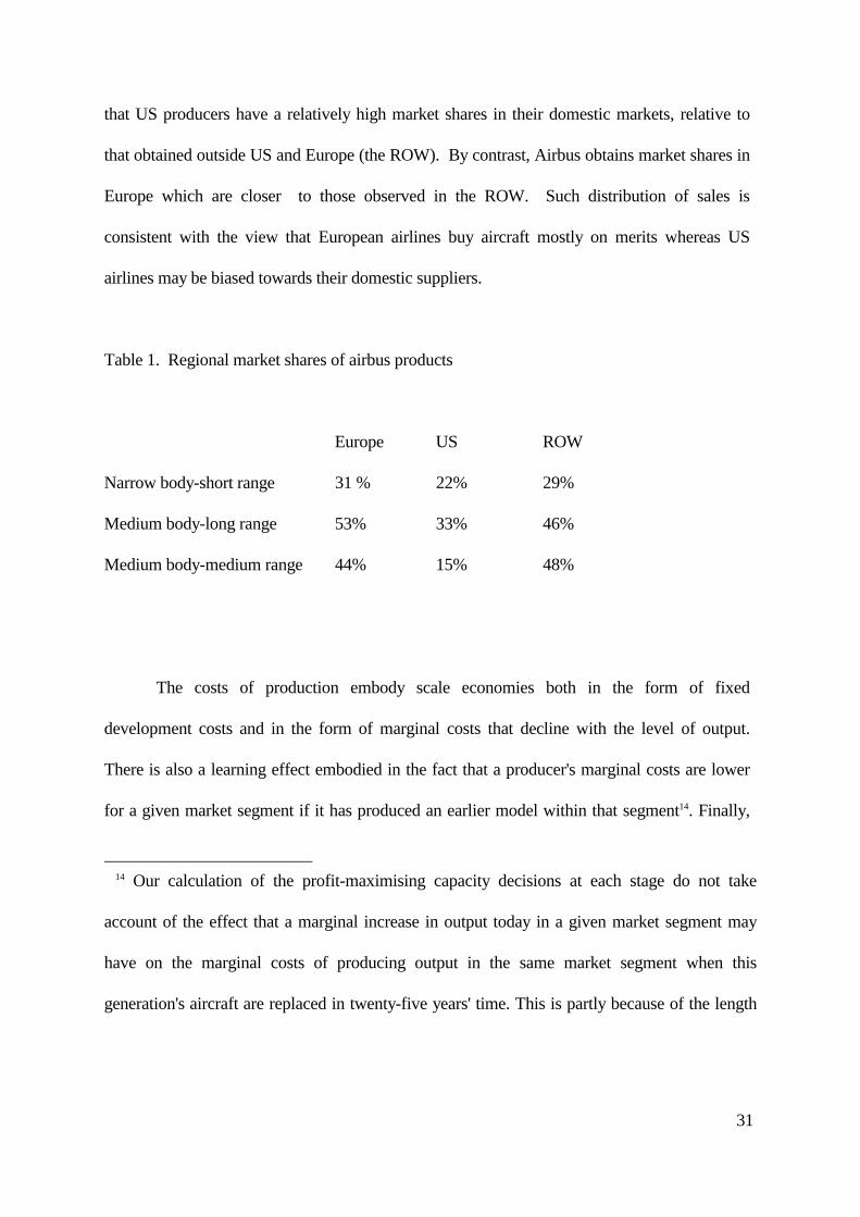
that US producers have a relatively high market shares in their domestic markets, relative to

that obtained outside US and Europe (the ROW). By contrast, Airbus obtains market shares in

Europe which are closer to those observed in the ROW. Such distribution of sales is

consistent with the view that European airlines buy aircraft mostly on merits whereas US

airlines may be biased towards their domestic suppliers.

Table 1. Regional market shares of airbus products

Europe US ROW

Narrow body-short range 31 % 22% 29%

Medium body-long range 53% 33% 46%

Medium body-medium range 44% 15% 48%

The costs of production embody scale economies both in the form of fixed

development costs and in the form of marginal costs that decline with the level of output.

There is also a learning effect embodied in the fact that a producer's marginal costs are lower

for a given market segment if it has produced an earlier model within that segment14. Finally,

14 Our calculation of the profit-maximising capacity decisions at each stage do not take

account of the effect that a marginal increase in output today in a given market segment may

have on the marginal costs of producing output in the same market segment when this

generation's aircraft are replaced in twenty-five years' time. This is partly because of the length

32

there are economies of scope in the form of marginal costs that decline with the level of output

produced in neighbouring segments.

The model is solved backwards. This means basically that the solution at each stage is

constrained by the requirement that predictions about the future must be consistent with

rational behaviour by all parties when those predictions are realised. What this implies is that

the model must not assume that producers were incapable of foreseeing developments which

the model itself predicts.

The steps involved in finding a solution are as follows. They consist of finding the

Nash equilibria consistent with a set of historical production data, and then checking to see

which of these Nash equilibria are sub-game perfect:

1) Parameter values are chosen for the whole model.

of time ahead (the average impact on the next generation's marginal costs takes place 37.5 years

from the present, which becomes negligible with even mild discounting). It is also because to do

so would introduce an arbitrary asymmetry between the calculation for our first two stages of

competition (A and B) where replacements are foreseen within our finite-horizon model, and

the remaining stages where it is not, although such replacement will almost certainly take place.

33

2) Using historical data about production in previous stages, the model calculates

the profit-maximising output in stage F under each combination of decisions by the three

players to enter the market or to stay out.

3) For each such combination it determines whether each of the parties would

make more profits by changing its entry decision15. If so, the combination is rejected as a non-

equilibrium. Any combinations that survive this test are listed as solutions. In principle there

might be multiple solutions: for instance, it might turn out to be profitable for only one

producer to enter a particular market segment, but for any of the three to able to do so as long

as the others stayed out. However, for our base run and all simulations only a single

combination of decisions has turned out to constitute a solution at each stage of the model.

4) The output values predicted for each producer by the solution to stage F are

used as parameters for the solution to stage E (stage E involves entry into a neighbouring

segment to that entered at stage F, so there are economies of scope as well as cross-elasticity

15 In the results we report producers do not discount future profits in making these entry

decisions. The reason for this is that under no reasonable calibration is MDD making a

comnmercial rate of return in the base run, so that to model the entry decisions as properly

discounted would make it difficult to calibrate the model consistently with MDD's presence in

the market. We have, nevertheless, compared our results with what would occur if proper

discounting were used and MDD were assumed to face counterfactually low fixed costs in the

base run; the qualitative results are very similar.

34

effects to take into consideration). We solve for an equilibrium at stage E taking as given the

predicted result at stage F as well as the historical values of output in stages A to D.

5) The procedure is repeated analogously for the other stages back to stage A.

6) We then check whether, at any stage, the equilibrium entry decision of any

producer would be different if, instead of historical output data, the equilibrium were

calculated using the outputs that would have been chosen if some producer X at an earlier stage

had made a non-equilibrium entry decision16. If so, we compare the total profits for producer X

under the two historical sequences and choose as the solution to the model the one that yields

the highest total profits.

We use the term "run" of the model to refer to a carrying out of steps 1) to 6) for a

given set of parameter values.

Each run of the model takes the characteristics (namely development and operating

costs) of aircraft types as given. However, it also calculates the optimal investment by each

manufacturer in product characteristics. For the base run the parameters of the function

determining investment levels are chosen so that manufacturers' historical investment levels

are the optimal ones given the output levels they produced. When running simulations under

16 Technically this amounts to ensuring that entry decisions at later stages are defined as

functions of earlier decisions.

35

alternative hypotheses, changes in outputs by the manufacturers are likely to alter the return to

investment in product characteristics and so change both the optimal level of investment and

the aircraft running costs that would result. Ensuring complete consistency between the

parameters of a run and their optimal values would require prohibitive computational resources

for comparatively little benefit. So in order to ensure approximate consistency the procedure

we have adopted is as follows. A simulation is run using the same parameters as the base case.

This generates a number of results including output levels and optimal investment levels,

which may be significantly different from historical levels of these variables that have been

used as parameters for the simulations. We therefore run a second simulation using among its

parameters the relevant variables generated by the first run. In the simulations we have

reported, the results of the second run are very similar to those of the first run, suggesting that

further attempts at convergence are unnecessary. This means that our results can be interpreted

as showing the impact of various alternative scenarios not just on physical volumes of output

produced but also on the quality of aircraft developed.

At two points in the model (stages D and F) at least one manufacturer is faced with a

choice between continuing to produce an existing model and producing a new or upgraded

model. Here our procedure has been to run a simulation under each of the two alternatives and

to compare the profits to the manufacturer in each outcome, reporting the more profitable

solution.

4. Results

36

In this section we report a comparison between prices and outputs at each stage of

development under various alternative hypotheses. First we report a "base run", which attempts

to reproduce fairly closely the history of the passenger aircraft market since the 1960s, and

reasonable current estimates of future demand. According to this base run, both Boeing and

MDD enter the SRNB and LRWB segments; Airbus and Boeing both produce MRMB aircraft

though MDD stays out; and all three producers enter the LRMB segment. We have also

conjectured that Airbus and Boeing (though not MDD) will decide to produce new LRWB

aircraft in the late 1990s. One important feature to note about the base case is that both Boeing

and MDD are assumed to foresee the later entry of Airbus even when making their initial

decision at stage A. This has the effect of making them produce slightly lower output since

they foresee that Airbus's presence will make it harder in the future to exploit economies of

scope between different models.

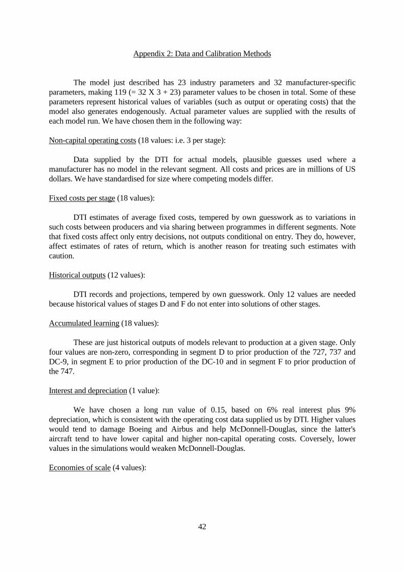
Appendix 2 reports the procedure we have used in calibrating those parameters of the

model about which we do not have direct data. To give some idea of the sensitivity of the

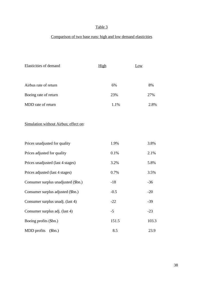
results to alternative values of the parameters, Table 3 shows two alternative base runs which

differ in respect of perhaps the hardest parameters to calibrate with confidence, namely

elasticities of demand. In principle elasticities are determined jointly by three variables: price,

output and the ratio of marginal cost to price at the equilibrium output. The former two are

given by historical data or forecasts, and the last is thought to lie somewhat below 60% (this is

a kind of stylised fact about which there is a rough industry consensus). However, because of

uncertainty about this last value we have calibrated a second base run with elasticities about

37

20% (in absolute value) higher than those given in the first. Subsequent tables will report the

figures based on the lower elasticities, because these are the ones that approximate better to the

consensus value of the price-marginal cost ratio; but the sensitivity of results to alternative

assumptions should be borne in mind. The most immediate impact of higher elasticities is to

lower the profitability of all producers: that of Airbus falls from 8% to 6%, and MDD barely

makes a positive rate of return. But in addition the effect of Airbus is weaker under high

elasticities; the percentage change in prices is roughly halved, and if induced quality changes

are taken into account the consumer surplus benefits of Airbus entry become negligibly small.

38

Table 3

Comparison of two base runs: high and low demand elasticities

Elasticities of demand High Low

Airbus rate of return 6% 8%

Boeing rate of return 23% 27%

MDD rate of return 1.1% 2.8%

Simulation without Airbus; effect on:

Prices unadjusted for quality 1.9% 3.8%

Prices adjusted for quality 0.1% 2.1%

Prices unadjusted (last 4 stages) 3.2% 5.8%

Prices adjusted (last 4 stages) 0.7% 3.5%

Consumer surplus unadjusted ($bn.) -18 -36

Consumer surplus adjusted ($bn.) -0.5 -20

Consumer surplus unadj. (last 4) -22 -39

Consumer surplus adj. (last 4) -5 -23

Boeing profits ($bn.) 151.5 103.3

MDD profits ($bn.) 8.5 23.9

39

A number of comments about the profitability calculations are in order. First, by "rate

of return" we mean the internal rate of return of the stream of revenues and costs accruing to

developing and manufacturing airframes in the four segments of the model; this is not the same

as the rate of return of the manufacturer on its capital employed, since the manufacturer will

typically have pre-existing overhead capital investments in addition to the development

expenditures incurred in respect of particular airliners. Secondly, with respect to Airbus we

have nevertheless sought to impute an capital cost to the development of its first aircraft which

can be thought of as the cost of setting up an aerospace operation over and above the cost to an

established operation of developing a new model. We have been extremely conservative in

this; a lower imputed capital cost, allied to lower elasticities, might raise Airbus's rate of return

to something like 11%, while lower capital costs in the presence of higher elasticities imply a

rate of return around 9%. Thirdly, we have assumed that manufacturers' revenues accrue at a

constant rate throughout the lifetime of each model; in practice this may overstate rates of

return since it does not allow for slow initial sales of new models. Finally, all of these estimates

are dependent on the forecasts of future demand and prices that have been used. More

pessimistic forecasts might significantly lower the rate of return to all producers including

Airbus. This is particularly important to bear in mind in the case of Airbus since most of its

profits in the base run occur after the mid-1990s. Figure 2 illustrates; it is worth noting for

comparison that the internal rate of return of Airbus's profit stream up to the mid-1990s is only

0.7%, even under the low elasticities assumption. Overall, we must stress that rates of return

are purely illustrative and should not be considered as forecasts.

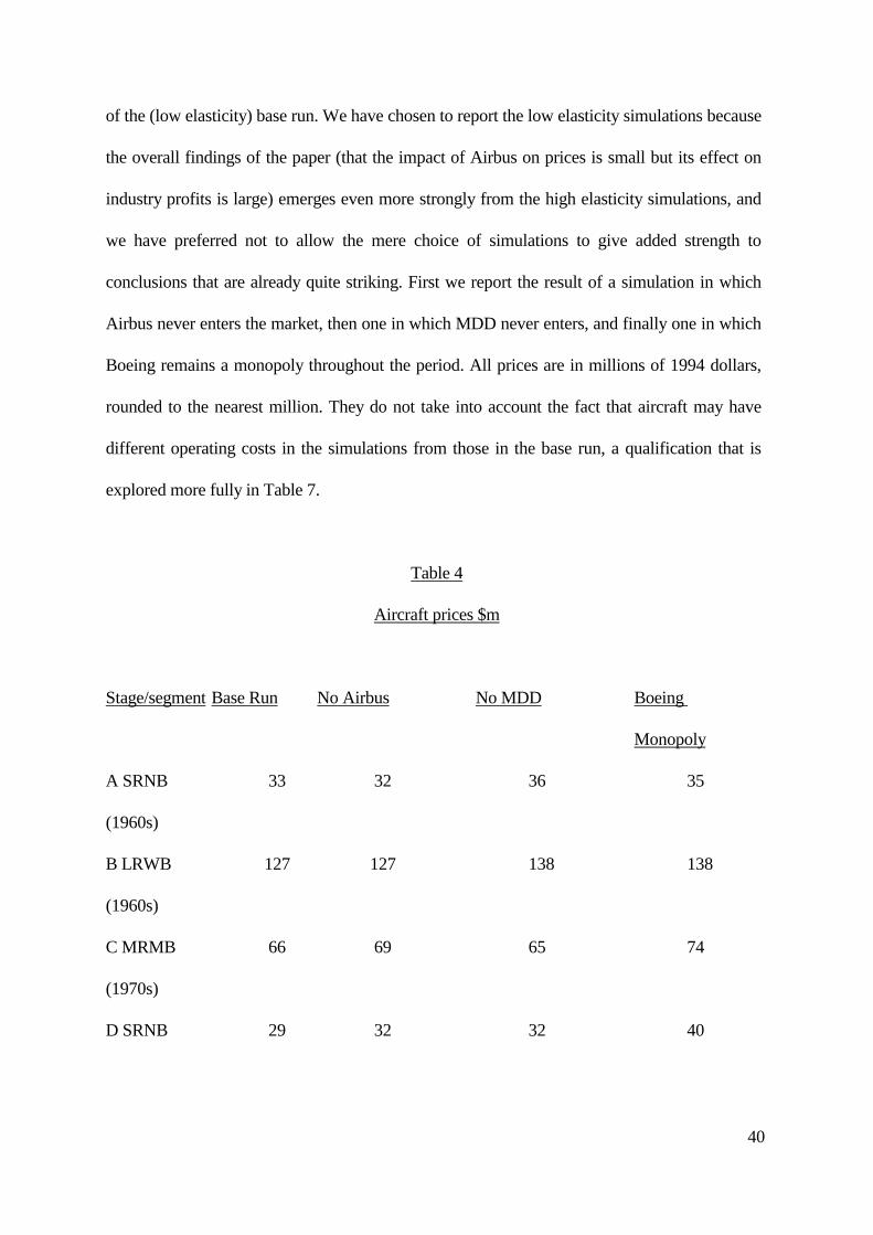
Table 4 reports aircraft prices under different alternative assumptions in addition to those

40

of the (low elasticity) base run. We have chosen to report the low elasticity simulations because

the overall findings of the paper (that the impact of Airbus on prices is small but its effect on

industry profits is large) emerges even more strongly from the high elasticity simulations, and

we have preferred not to allow the mere choice of simulations to give added strength to

conclusions that are already quite striking. First we report the result of a simulation in which

Airbus never enters the market, then one in which MDD never enters, and finally one in which

Boeing remains a monopoly throughout the period. All prices are in millions of 1994 dollars,

rounded to the nearest million. They do not take into account the fact that aircraft may have

different operating costs in the simulations from those in the base run, a qualification that is

explored more fully in Table 7.

Table 4

Aircraft prices $m

Stage/segment Base Run No Airbus No MDD Boeing

Monopoly

A SRNB 33 32 36 35

(1960s)

B LRWB 127 127 138 138

(1960s)

C MRMB 66 69 65 74

(1970s)

D SRNB 29 32 32 40

41

(1980s)

E LRMB 102 113 106 114

(1980s)

F LRWB 125 126 125 143

(1990s)

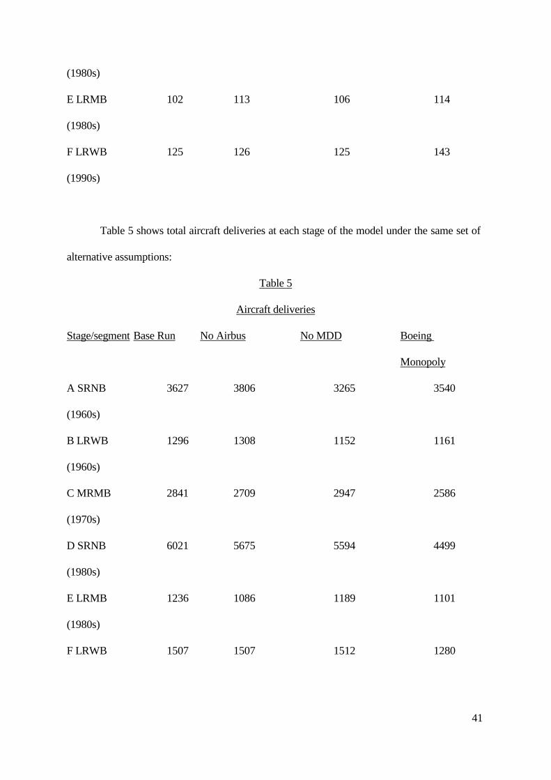
Table 5 shows total aircraft deliveries at each stage of the model under the same set of

alternative assumptions:

Table 5

Aircraft deliveries

Stage/segment Base Run No Airbus No MDD Boeing

Monopoly

A SRNB 3627 3806 3265 3540

(1960s)

B LRWB 1296 1308 1152 1161

(1960s)

C MRMB 2841 2709 2947 2586

(1970s)

D SRNB 6021 5675 5594 4499

(1980s)

E LRMB 1236 1086 1189 1101

(1980s)

F LRWB 1507 1507 1512 1280

42

(1990s)

Table 6 overleaf shows the percentage changes in prices under the different

simulations, unadjusted for quality differences (which are shown in Table 7). Note that the

absence of Airbus actually lowers prices in Stage A, even though Airbus does not enter in

Stage A in the base run. This is because Boeing anticipates a higher output in a neighbouring

segment (the medium body, medium range segment at stage C); because of larger spillovers

across segments, Boeing has therefore a stronger incentive to expand output at stage A.

However, once Airbus actually enters the market (from Stage C onwards) it has an

unambiguously downward impact on prices.

Note also that the absence of MDD lowers prices in the MRMB segment (in which

MDD has no presence in the base run). This is because MDD's absence from the two

neighbouring segments enables the other producers to realise more economies of scope and so

lower prices.

The absence of Airbus in almost all cases results in the other manufacturers making

higher investments in operating efficiency. This is because the return to such investments rises

as the manufacturers are able to realise savings in operating costs over a higher level of output.

However, Airbus's absence also deprives consumers of access to Airbus's aircraft, which have

lower fuel and maintenance costs than MDD's, so not all customers purchase more fuel-

efficient aircraft in the absence of Airbus.

43

Table 6

Changes in Aircraft prices compared to Base Run

Unadjusted for quality

Stage/segment No Airbus No MDD Boeing

Monopoly

A SRNB - 3% + 7% + 4%

(1960s)

B LRWB 0 + 9% + 9%

(1960s)

C MRMB + 5% - 2% + 12%

(1970s)

D SRNB + 8% + 9% + 36%

(1980s)

E LRMB + 11% + 3% + 11%

(1980s)

F LRWB + 1% 0 + 15%

(1990s)

44

Table 7

Changes in Aircraft prices compared to Base Run

Adjusted for quality

Stage/segment No Airbus No MDD Boeing

Monopoly

A SRNB - 3% + 7% + 3%

(1960s)

B LRWB 0 + 7% + 7%

(1960s)

C MRMB + 3% - 2% + 10%

(1970s)

D SRNB + 8% + 9% + 35%

(1980s)

E LRMB + 3% + 1% + 3%

(1980s)

F LRWB + 1% 0 + 11%

(1990s)

45

Full details (including results and parameter values) of the base run and No Airbus

simulation are given in Appendix 4. Three features of the simulation in particular are worth

noting:

1) The absence of Airbus encourages MDD to enter segment 2 with a direct

competitor to the Boeing 737.

2) The absence of Airbus discourages MDD from producing the MD-11. This is

because Boeing can now reap sufficient scale economies to be able to price the 777 at a level

against which MDD is unable to compete. Note that this is the contrary to the view expressed

in the mid-1980s that entry by Airbus would discourage entry by MDD (see Vickers, 1985, and

the various arguments in Dixit & Kyle, 1985 and Geroski & Jacquemin, 1985). This view

proved to be mistaken, and the current model suggest why. Airbus's entry actually made life

easier for MDD because its sales reduced Boeing's economies of scale.

3) The base run has Airbus deciding in the late 1990s to produce a direct

competitor to the 747. Obviously this is dependent on precise demand projections. Given the

ones we have used, Airbus entry would keep MDD out of this segment.

5. Implications for benefits to consumers and producers

46

The prices and outputs reported in the simulations can be used to calculated changes in

aggregate consumer surplus17 (this means overall benefits to airlines, and it is a further question

to what extent such benefits might be passed on to passengers). For the No Airbus case these

amount to approximately a reduction of $36 bn, or a reduction of $20 bn if quality differences

are taken into account18. For the Boeing monopoly case they amount to a reduction of just over

$118 bn (quality-adjusted). For comparison, without Airbus total profits in the industry would

be some $68 billion higher over the whole 60-year period, and under a Boeing monopoly they

would be $290 billion higher.

The reason why Airbus does not have a larger impact on prices is that the pro-

competitive effects of entry are offset by a weakening of the competitive pressure from MDD,

and reduced learning economies for both existing manufacturers (especially Boeing). Our

17 These are measured as the area of the trapezium in a demand-supply diagram bounded by

the demand curve and the two price lines (before and after the change). Since demand curves

are linear in this model this area can be measured precisely.

18 If one includes only the impact on consumer benefits in those segments in which Airbus has

a presence, the figure for the consumer benefits due to Airbus entry is $26 bn instead of $20 bn.

This is because the model assumes that other producers produced less at stages A and B in

anticipation of Airbus's entry. This assumption may be thought unrealistically strong, in which

case the figure of $26 bn may be a more appropriate one. However, it should be noted that under

the high elasticities assumption this could fall to as low as $5 bn.

47

estimates of these effects are obviously dependent on the parameter values chosen, but we have

endeavoured to use a realistic value in the light of the industry consensus.

One final question we can use to model to answer is what would have been the

consequences of a "wrong" decision by Airbus. In the base run entry by Airbus in the late

1960s with a rival to the Boeing 747 would be unprofitable. But suppose European

governments had picked a loser? How bad would it have been? The answer is that the decision

would have resulted in losses of about $3.5 billion, sufficient to bring Airbus's overall rate of

return over the whole period down from 8% to 6%. The impact on the overall market would

have been negligible, since in that event (according to our simulations) MDD would not have

developed the DC-10, and the two events would to all intents and purposes have cancelled

each other out. So it would have been regrettable but scarcely a disaster. This is worth bearing

in mind in the light of claims that failed government support can be very costly. For example,

Helpman & Krugman (1989) write: "It is possible to believe that imperfect competition is

pervasive while at the same time believing that the imperfections associated with it are fairly

modest and the gains from optimal deviations from free trade small. Again, the quantitative

work reported in chapter 8 seems to confirm this. One can always do better than free trade, but

the optimal tariff or subsidies seem to be small, the potential gains tiny, and there is plenty of

room for policy errors that may lead to eventual losses rather than gains". What the present

model suggests is that losses resulting from failures of strategic trade policy, while certainly

counting as losses, may also be quite small. Strategic trade policy may sometimes be both less

effective than its friends would hope and less dangerous (from a narrow nationalistic

48

perspective) than its enemies fear. In this model the entry of Airbus is bad for the world as a

whole, but not particularly dangerous for its backers in Europe.

6. How robust are the findings?

Two qualitative findings emerge very clearly from our model under any reasonable

variation or re-calibration that respects its fundamental structure. First, the impact of Airbus

entry on consumer surplus is modest; and secondly, its impact on Boeing's profits is large.

The particular reaction of MDD to Airbus entry is quite sensitive to the details of

model specification. For example, it would take only a small change in the parameters to

ensure that MDD did not produce a rival to the Boeing 737 even if Airbus had never produced

the A-300. Likewise, a small change in parameters (a reduction in the scope parameter, for

example) would mean that MDD still continued to produce the MD-11 even in the absence of

Airbus. However, a more general qualitative result is highly robust. The reaction of MDD (the

weaker rival) to Airbus's entry is the net outcome of two factors that tend in opposite

directions: the direct effect of the Airbus presence in lowering aircraft prices, and the indirect

effect in weakening Boeing and thereby raising aircraft prices. This second effect, which if

sufficiently large can give rise to the Starfish phenomenon, is an important factor in all

reasonable specifications of the model even if it is not always the determinant one.

49

The Starfish effect continues to be observed in the high elasticities simulation as well as

that reported using low elasticities (that is, MDD does not produce the MD-11 in the absence

of Airbus). In general the impact of Airbus on prices is weaker when elasticities are high. This

is what one would expect since under these conditions a monopoly or duopoly is less able to

exploit market power. This increases the risk that the pro-competitive effect of Airbus entry

might be outweighed by its adverse impact on the ability of other producers to exploit scale

economies and on their incentive to make R&D investments. Indeed our simulations with high

elasticities reveal a slight negative impact of Airbus entry on (quality-adjusted) prices in the

two medium-range segments (occupied by the A-300 and the A-330/A-340). While we should

not put undue weight on these findings, they do indicate that even the weak impact of Airbus

on prices in our main simulations may be overstated.

The model's qualitative findings are certainly sensitive to assumptions about the likely

course of future demand. This is in contrast to the conjecture that has sometimes been made

about this industry that increased investment in product development would outweigh any

effect of demand expansion and thereby ensure that the market was always likely to be

dominated by one or two producers (see Sutton, 1987). Our results indicate that the indirect

effect of demand expansion on fixed investment is nothing like enough to outweigh the direct

effect of demand expansion. In consequence, how many manufacturers the market can

profitably support will always be sensitive to demand projections.

50

There are four respects in which the model's findings may be sensitive to the model's

structure rather than to its specific parameters. First, the model assumes that the only impact of

competition on production costs is by affecting manufacturers' output levels and thus their

ability to reap scale and learning economies. We have not allowed for the possibility that

competition may act as a direct spur to increased efficiency in production methods. There is no

professional consensus about how to model such effects, but there is evidence that they may be

important in some industries. It is likely that taking such phenomena into account would

increase the effect of Airbus entry in lowering aircraft prices.

Secondly, our modelling of production decisions assumes that production capacity is

decided once and for all at the start of a model's production cycle and cannot be subsequently

changed. While this assumption is clearly unrealistic, it is not clear what effect a more realistic

assumption would have on the model's results.

Thirdly, the fact that we ignore the possible strategic motivation for capacity choices

(unlike that for entry decisions) may slightly affect both the calibration of the base run and the

nature of the simulations. The only plausible strategic motivations we have ignored are ones in

early stages that affect subsequent marginal entry decisions by MDD at either stage E or Stage

C, or ones that affect output decisions at stage D. Ignoring these last may mean we have

slightly underestimated the marginal cost of producing the Boeing 737 (because we have

treated actual output as equal to the Cournot output, instead of as exceeding the Cournot output

by an amount designed to induce output reductions by rivals at a later stage); ad hoc simulation

51

suggests this would make a very small difference to the overall results, and that the linear

specification of our model may even exaggerate this difference.

Alternatively, the base run may underestimate the marginal cost of producing the DC-10,

since additional output of the DC-10 beyond the static profit-maximising level might have

contributed to the learning economies that made the decision to develop the MD-11 at stage E

just profitable. It is conceivable also that Boeing may have produced larger numbers of SRNB

aircraft at Stage A than would otherwise have been profitable, in order to deter entry by MDD

at Stage C (where MDD did not in fact enter). Either effect would imply that the presence of

Airbus encourages strategic increases in output at earlier stages because of Airbus's tendency

to weaken MDD and make its entry decisions more marginal; this effect would counteract that

already noticed, in which the knowledge of Airbus's subsequent entry restrains output by

Boeing and MDD at stages A and B because of the anticipated loss of scale and scope

economies. Ignoring the strategic motive for capacity-setting in the simulations, however,

would only really matter as far as MDD's predicted entry at Stage C (with a rival to the Boeing

737) is concerned. It is possible that, in the anticipated absence of Airbus, Boeing might have

wished to produce more SRNB aircraft to deter entry by MDD. This effect works in the

opposite direction from the previous two. And all these effects concern the impact of Airbus on

output at Stages A or B - that is, before Airbus's actual entry. Since there is some doubt in any

case to what extent Boeing and MDD really foresaw so early the subsequent development of

the consortium, it seems to us that the quantitative impact of our ignoring strategic motivations

for capacity-setting is most unlikely to be important.

52

Finally, our modelling of investment in aircraft quality is undoubtedly simplistic.

Producers are supposed to maximise profits by choosing a point on a differentiable technology

production function that yields aircraft operating costs as a function of fixed development

costs. This overlooks the possibility that investment may be subject to indivisibilities, and

more profoundly ignores the possibility of R&D expenditures' arising partly out of non-

maximising managerial behaviour: if incentives for R&D expenditure arise more out of threats

to existing profits than out of the prospect of making more, then Airbus may have had a more

beneficial effect on innovation in the industry than our model implies. Furthermore, since

aircraft in a given segment are identical except with regard to operating costs this implies that

all development expenditures by different producers within a segment represent pure

duplication. Given the fact that there is still some differentiation of aircraft even within

segments, once again our methodology may paint an unwarrantedly negative picture of the

impact of Airbus on this market. Quantifying the extent of any bias is, however, a much more

difficult task.

8. Concluding remarks

This paper has modelled the impact of Airbus on the market for large jet aircraft. What

have we learned? Most importantly we have learned that an entrant facing two asymmetric

rivals is in a quite different situation from an entrant facing a single incumbent. Airbus has had

a much less significant effect on prices and outputs in this market than earlier duopoly models

had led us to expect. We have also learned that entry deterrence involves delicate calculations;

when rivals are asymmetric there is a serious danger of the Starfish effect.

53

In the light of these sober lessons it is encouraging and perhaps surprising that Airbus is

not Concorde: it has a reasonable chance of making a good if not spectacular profit. This profit

has been bought at the considerable expense of the shareholders of the Boeing Corporation and

(perhaps) the taxpayers of the United States. It is not surprising that they have objected; given

the sums of money at stake it is perhaps more surprising that there have not been more

determined efforts to sponsor transatlantic collusion.

54

Bibliography

Baldwin and Flam (1989): "Strategic trade policies in the market for 30-40 seat commuteraircraft", Weltwirstschaftliches Archiv, 125 (3), 484--500.

Baldwin, R. &P. Krugman (1987): « Market Access and International Competition : A simulation

Study of 16K Random Access Memory » in Robert Feenstra(ed.),

Empirical Research in International Trade, Cambridge, Mass, 171-197.

Baldwin, R. & P. Krugman (1988): "Industrial Policy and International Competition in Wide-

Bodied Jet Aircraft", in Baldwin, R.E (ed): Trade Policy Issuesand Empirical Analysis, Chicago, University of Chicago Press.

Brander, J. & B. Spencer (1985): « Export subsidies and international market share rivalry »,

Journal of International Economics, 18, 83-100

Dixit, A. & A, Kyle (1985): "The Use of Protection and Subsidies for Entry Promotion and

Deterrence", American Economic Review, 75, 139-152.

Geroski, P. & A. Jacquemin (1985): "Corporate Competitiveness in Europe", Economic Policy, 1,

170-205.

Helpman, E. & P Krugman (1989): Trade Policy and Market Structure, Cambridge, MIT Press.

Klepper, G. (1990): "Entry into the Market for Large Transport Aircraft", EuropeanEconomic Review, 34, 775-803.

Klepper, G. (1994): « Industrial policy in the transport aircraft industry », in P. Krugman and A. Smith, eds, Empirical studies of StrategicTrade Policy, NBER, University of Chicago Press, Chicago

Kreps, D. & J. Scheinkman (1983): "Quantity Precommitment and Bertrand Competition Yield

Cournot Outcomes", Bell Journal of Economics, 14, 326-337.

Matutes, C. &Pierre Regibeau: « A selective survey of the Economics of Standardization entry

55

deterrence, technological progress and internationalcompetition », European Journal of Political Economy,forthcoming

Sigmund. K. (1993): Games of Life, Harmondsworth, Penguin Books.

Stein, J. (1989): "Efficient Capital Markets, Inefficient Firms: a model of myopic corporate behavior", Quarterly Journal of Economics, 104, 655-

69

Stokey, N. (1981): « Rational expectations and durable goods pricing », BellJournal of Economics, XII (Spring), 112-128.

Sutton, J. (1987): « Sunk Costs and Market Structure », MIT Press.

Sutton, J. (1995): « One Smart Agent », mimeo, LSE

Tyson, L. (1992): « Who is bashing whom ? Trade conflict in High-Technologyindustries », Institute for International Economics, WashingtonDC.

Vickers, J. (1985): "Discussion of Geroski & Jacquemin", Economic Policy, 1,205-211.

Wilson, E. O. (1993): The Diversity of Life, Harmondsworth, Penguin Books.

Appendix 1: The Structure of the Model

A.1.1 Definitions and Equations

There are 4 market segments, indexed i=1,..,4:

1) Short-range, narrow bodied (A 320, B 737, MD-80)

2) Medium range, medium bodied (A 300/310, B 757, B 767)

3) Long-range, medium bodied (A 330/340, B 777, MD-11))

4) Long-range wide bodied (B 747)

Producers are Airbus, Boeing and McDonnell-Douglas, indexed j=1,2,3.

Demand is linear, and chain linked, i.e. there is substitution between products in onesegment and those in neighbouring segments:

(1) kij + mij = ai + biqi + ci(qi+1 + qi-1)

where:

kij represents the annual capital cost to the airline of running the aircraft;

mij represents other costs (basically fuel and maintenance);

qi is total output in segment i.

Note that for segments 1 and 4, one of the two neighbouring segments has demand identicallyequal to zero.

kij is in turn a function of the price of the aircraft:

(2) kij = pij(r + D)

where:pij is the price of the aircraft;r is the real interest rate;D is the depreciation rate;

37

Equations (1) and (2) together yield an expression for the price of the aircraft:

(3) pij = [ai + biqi + ci(qi+1 + qi-1) - mij]/(r + D)

Costs are likewise linear, and display scale, learning, chain-linked scope and vintageeffects:

(4) Cj = Fj + (α1j - Γ(Q2j+q2j))q1j + (β1-δQ1j)(q1j)2

+ (α2j - Γ(Q1j+q1j+Q3j+q3j))q2j + (β2-δQ2j)(q2j)2

+ (α3j - Γ(Q2j+q2j+Q4j+q4j))q3j + (β3-δQ3j)(q3j)2

+ (α4j - Γ(Q3j+q3j))q4j + (β4-δQ4j)(q4j)2

where:

Cj is the total cost of production by producer j.

Fj is the fixed cost of production by producer j (which is a function of the segments inwhich it operates).

αij is a vintage-specific cost parameter for the model produced in segment i by producerj (capturing the idea that the cost of production of a model may depend on factorspeculiar to its vintage).

Qij represents cumulative output in segment i by producer j (to capture learning effects).

Γ and δ represent respectively scope and learning parameters.

38

A.1.2 Solving the Model

We can use equations (3) and (4) to formulate a profit function which will then bedifferentiated with respect to output. In principle, since output in one segment affects prices(and therefore profit) in neighbouring segments, we should differentiate the global profitfunction for all segments considered together. In practice, to simplify notation we can define theincremental profit function for producer j in segment i as those components of profit insegments i-1, i and i+1 considered together that are affected by output in segment i:

(5) πij = qij [ai + biqi + ci(qi+1 + qi-1) - mij]/(r + D)

+ qi-1,j [ai-1 + bi-1qi-1 + ci-1(qi + qi-2) - mi-1,j]/(r + D)

+ qi+1,j [ai+1 + bi+1qi+1 + ci+1(qi+2 + qi) - mi+1,j]/(r + D)

- Fij - (αij - Γ(Qi-1,j+qi-1,j+Qi+1,j+qi+1,j))qij + (βi-δQij)(qij)2

- (αi-1,j - Γ(Qi-2,j+qi-2,j+Qij+qij))qi-1,j

- (αi+1,j - Γ(Qi+2,j+qi+2,j+Qij+qij))qi+1,j

where Fij is the incremental fixed cost associated with entry by producer j into segment i.

Differentiating (5) with respect to qij yields:

(6) dπij/dqij = [ai + biqi + ci(qi+1 + qi-1) - mij]/(r + D)

+ [biqij + ci-1qi-1,j + ci+1qi+1,j]/(r + D)

- (αij - Γ(Qi-1,j+qi-1,j+Qi+1,j+qi+1,j))

- 2qij(βi-δQij)

+ Γ(qi-1,j+qi+1,j)

Setting equation (6) equal to zero for j=1,2,3 and substituting qi=qi1+qi2+qi3 yields asystem of simultaneous equations in the three variables qi1,qi2 and qi3. This system is verylengthy to solve by hand, so we have used a Mathematica programme to do so. The solutionsare described in Appendix 3.

Essentially this solution technique involves assuming that the output decision in eachsegment is taken simultaneously by the three producers, with each one treating as parametric itsown (historically given) past and (rationally anticipated) future output in other segments, as well

39

as the output of its competitors in all segments. This latter is the Cournot assumption, whichKreps and Scheinkman (1983) have shown is a reasonable approximation to a form ofcompetition in which producers first choose production capacity and then compete in prices.

There are six stages of the model, which correspond to a stylised account of the historyof the civil airliner market from the mid-1960s to the late 1990s. At each stage producers chooseonce and for all the level of production capacity (i.e. output) over the 25-year life of the modelproduced:

A (early 1960s): The players decide whether to enter segment 1 [this corresponds to the decisionby Boeing to produce the 727 and 737, and by MDD to produce the DC-9]

B (late 1960s): Segment 4 [Boeing 747, MDD DC-10]

C (1970s): Segment 2 [Airbus 300,310, B 757,767]

D (early 1980s): Segment 1 [Airbus 320, B 737, MD-80]

E (late 1980s): Segment 3 [A-330,340, B 777, MD-11]

F (late 1990s): Segment 4 [replacements for the 747?]

The model is solved backwards, in the following way. First stage F is solved, taking asparametric the (historically given) value of output in the other segments. Then stage E is solved,taking the historical value of output in stages A-D and the equilibrium value of output in stage F(and so on analogously for other stages). We then check whether, at any stage, the equilibriumentry decision of any producer would be different if, instead of historical output data, theequilibrium were calculated using the outputs that would have been chosen if some producer Xat an earlier stage had made a non-equilibrium entry decision. If so, we compare the total profitsfor producer X under the two historical sequences and choose as the solution to the model theone that yields the highest total profits.

For the base run, which attempts to reproduce history, there is by definition a fairly closecorrespondence between historical and equilibrium values of output. For counterfactualsimulations, we have undertaken a first run from which we extract equilibrium output valuesthat are then entered as historical values in the second run; the results of the two runs are usuallyvery similar, indicating that the model converges rapidly.

There are two small qualifications to the temporal structure of the model. One is thatproduction in the different market segments is not simultaneous, so that cross-elasticities are notstrictly valied for the whole production run of a model. The solution we have adopted is thefollowing. Stages C and E (corresponding to segments 2 and 3) overlap with both an earlier anda later stage in which productions are made in a neighbouring segment (decisions in Stage Coverlap with production in stages A and D; decisions in stage E overlap with production in

40

stages B and F). Prices in these segments are determined as the weighted average of the pricesthat would obtain if there were full overlap with either of the two relevant stages. The weightsare parameters lambda2 and lambda3, which can be interpreted as the proportion of its life thataircraft in segments 2 and 3 respectively will be competing against the earlier model in aneighbouring segment as opposed to competing against the replacement models. At other stageswe have assumed full overlap, but have chosen relatively modest cross-elasticities to relfect thefact that in practice there will be competition from neighbouring segments only for some of amodel's lifetime.

The second temporal qualification is that we have treated the introduction of the DC-10as belonging to segment 4 (instead of segment 3 where it would more naturally belong). This isto avoid introducing an additional decision in segment 3 earlier in the model, which wouldconsiderably increase the computational complexity of the model while yielding little newinsight. However, we have assumed that learning economies were utilised by McDonnell-Douglas in building the MD-11.

A.1.3 Endogenising Product Development

The model can also be used to endogenise expenditure on research and development, bymaking operating costs of the aircraft a function of fixed development costs, and examining theway in which different hypotheses about market structure affect the incentives of manufacturersto invest in reducing these costs. To do this we differentiate equation (5) with respect to Fij.Setting the derivative equal to zero, we can appeal to the envelope theorem to ignore any effectof changing fixed costs on the optimal value of qij when small changes are considered. Thisprocedure yields:

(7) dπij/dFij = -qij[dmij/dFij]/(r+D) - 1 = 0

Multiplying by Fij/mij gives the equilibrium level of fixed costs:

(8) Fij = qij.mij.hij/(r+D)

where hij is the (absolute value of the) elasticity of aircraft operating costs with respect to fixedcosts.

Solving (8), which has two unknowns, requires choosing a function relating Fij to mij. We havechosen for simplicity a constant elasticity cost function:

(9) m = k(F)-h

41

where subscripts are omitted for notational convenience. Substituting (9) in (8) yields anexpression for F*, the optimal value of F:

(10) F* = (kqh/(r+D))H,

where H = 1/(1-h).

It is worth noting that the choice of a constant elasticity form (coupled with thecalibration methods we discuss below) probably somewhat exaggerates the incentive formanufacturers to make investments in reducing operating costs; it has been suggested to us thatthe elasticity probably falls as development costs rise. However, since the qualitative results wereport do not differ according to whether or not we endogenise development costs, the fact thatthe true value of endogenous development costs may lie somewhere between the two casessuggests the model's findings are fairly robust to this modification.

We have used the same method for incorporating cost endogeneity in our counterfactualsimulations as for incorporating output variation. That is, we run a simulation with changedparameters, observe the endogenous costs and then run a second simulation with those costsentered as new parameters and report the results of the second run; again the difference betweenfirst and second runs is usually small.

42

Appendix 2: Data and Calibration Methods

The model just described has 23 industry parameters and 32 manufacturer-specificparameters, making 119 (= 32 X 3 + 23) parameter values to be chosen in total. Some of theseparameters represent historical values of variables (such as output or operating costs) that themodel also generates endogenously. Actual parameter values are supplied with the results ofeach model run. We have chosen them in the following way:

Non-capital operating costs (18 values: i.e. 3 per stage):

Data supplied by the DTI for actual models, plausible guesses used where amanufacturer has no model in the relevant segment. All costs and prices are in millions of USdollars. We have standardised for size where competing models differ.

Fixed costs per stage (18 values):

DTI estimates of average fixed costs, tempered by own guesswork as to variations insuch costs between producers and via sharing between programmes in different segments. Notethat fixed costs affect only entry decisions, not outputs conditional on entry. They do, however,affect estimates of rates of return, which is another reason for treating such estimates withcaution.

Historical outputs (12 values):

DTI records and projections, tempered by own guesswork. Only 12 values are neededbecause historical values of stages D and F do not enter into solutions of other stages.

Accumulated learning (18 values):

These are just historical outputs of models relevant to production at a given stage. Onlyfour values are non-zero, corresponding in segment D to prior production of the 727, 737 andDC-9, in segment E to prior production of the DC-10 and in segment F to prior production ofthe 747.

Interest and depreciation (1 value):

We have chosen a long run value of 0.15, based on 6% real interest plus 9%depreciation, which is consistent with the operating cost data supplied us by DTI. Higher valueswould tend to damage Boeing and Airbus and help McDonnell-Douglas, since the latter'saircraft tend to have lower capital and higher non-capital operating costs. Coversely, lowervalues in the simulations would weaken McDonnell-Douglas.

Economies of scale (4 values):

43

In each segment we have chosen a parameter that gives, at the mean value of output, anapproximation to the view, widely accepted in the industry, that a doubling of output would beexpected to yield a 20% fall in marginal costs of production.

Economies of scope (1 value):

Here there is no comparable industry consensus that we have been able to ascertain. Wehave chosen a linear approximation to the two values of the scope parameter of Klepper (1990),using his higher value of 0.0033 for our base case.

Economies of learning (1 value):

The parameter here is chosen to approximate the view that a 100% increase inaccumulated production leads to a 20% saving in variable cost. The main effect of alternativevalues is on prices in segment D, where lower values lead to slightly higher prices in thealternative simulations but leave the base run unaffected.

Marginal production costs (12 values):

The intercept of the marginal cost curve is specific to each segment and each producer(changes in marginal costs between different stages of segments 1 and 4 are in effect capturedby changes in the values of m). We have chosen these values so that, at equilibrium outputs,variable costs are approximately equal to 60% of historical revenues, in line with the industryconsensus on the division of costs into fixed and variable components. However, aftercalibration of the demand function (see below) we have then adjusted the relative values of αijwithin each stage so as to reproduce approximately the historical market shares. The values ofαij can then be interpreted as embodying not only marginal costs of production as such but alsoany differences in manufacturers' ability to produce to customers' specifications (such asdifferences in perceived reliability, convenience etc.).

Own-price demand coefficients (4 values):

Once the marginal cost curve is determined, calibration to historical output levelsdetermines the point of intersection of the marginal cost and marginal revenue curves, andcalibration to historical prices determines the slope of the marginal revenue curve (and hence, ina linear model, the demand curve).

Demand intercepts (6 values):

These are determined by the same process that determines the own-price elasticities.Note, however, that intercepts may differ between stages A and D, and between B and F, sincehistorical outputs differ, but we have constrained price coefficients to be the same.

Cross-price demand coefficients (4 values):

44

Lacking either data on these or an effective means of calibration we have chose them tolie at between 10% and 5% of the own-price values. This reflects a view that aircraft inneighbouring segments are a fairly poor substitute for one another, at least over the range ofprice variation under consideration here. This does not mean, however, that cross-price effectsare unimportant, since they may affect the profitability of an entry decision. Setting all cross-price effects to zero in our base run induces entry by McDonnell-Douglas at stage C, since nowthe aircraft produced in segment 2 have no depressant effect on the prices of the MD-80 and theMD-11.

Lambda (2 values):

Chosen at 0.3 and 0.5 to capture degree of historical overlap between stages.

Elasticities of operating costs with respect to development costs (18 values):

For each producer at each stage, h is chosen approximately to satisfy equation (8) withrespect to historical outputs and fixed costs. In other words it is assumed that producers wereoptimising in choosing their development costs. The value of k is then chosen to satisfyequation (9) for historical levels of operating costs. Equation (10) then determines optimal fixedcosts, which will by definition be approximately equal to actual fixed costs for the base run. Forsimulations, (10) and (9) determine the optimal fixed and operating costs respectively.

45

Appendix 3

Solutions to First Order Conditions

The following are the solutions generated by Mathematica to the system of first order conditionsdescribed in Appendix 1:

3 PLAYERS

qi3: (-((bi*A2-bi*A3)*(bi2-2*bi*B1))+C2*(bi*A1-2*A3*B1))/E2

qi2: (-((bi*A1-bi*A2)*(bi2-2*bi*B3))+C1*(bi*A3-2*A2*B3))/E1

qi1: (-((bi*A3-bi*A1)*(bi2-2*bi*B2))+C3*(bi*A2-2*A1*B2))/E3

where:

Aj= -ai+mij-ci*qi-1-ci-1*qi-1,j-ci*qi+1-ci+1*qi+1,j+αij*(r+D)-2*Γ*qi-1j*(r+D)-Γ*Qi-1,j*(r+D)-2*Γ*qi+1,j*(r+D)-Γ*Qi+1,j*(r+D)

Bj= bi-βi*(r+D)+δ*Qij*(r+D)

Cj= bi2-2*βi*bi*(r+D)+2*bi*δ*Qij*(r+D)

Ej=(-((bi2-2*bi*Bj-1)*(bi

2-2*bi*Bj+1))+Cj*(bi2-4*Bj-1*Bj+1))

and where B0=B3 and B4=B1.

2 PLAYERS

qi2=(biA1-2*A2B1)/(bi2-4*B1B2)

qi1=(biA2-2*A1B2)/(bi2-4*B1B2)

where,

Aj=(-ai+mij-ci*qi-1-ci-1*qi-1,j-ci*qi+1-ci+1*qi+1,j+αij*(r+D)-2*Γ*qi-1,j*(r+D)-Γ*Qi-1,j*(r+D)-2*Γ*qi+1,j*(r+D)-Γ*Qi+1,j*(r+D))

Bj= (bi-βi*(r+D)+δ*Qij*(r+D))

46

1 PLAYER

qij=A *(B+C)

where,

Aj= [(2bi)/(r+D)-2*(βi-δ*Qij)]-1

Bj= (-ai+mij-ci*(qi+1+qi-1)-ci-1qi-1,j-ci+1qi+1,j)1/(r+D)

Cj= αij-Γ*(Qi+1,j+2qi-1,j+2qi+1,j+Qi-1,j)

The solutions in the three-player case are hard to interpret intuitively. However, it ishelpful to begin from the one-player case. The term (B+C) is essentially a measure of how farapart are the intercepts of the monopolist's marginal cost and marginal revenue curves (Bdefining the marginal revenue and C the marginal cost, taking cross-effects into account). Theterm A measures the difference in slope between the two curves (which depends on theelasticity of demand but also on the degree of scale economies) and consequently determinesat what level of output they will intersect.

The equations in the two-player and three-player cases use the same principle but appliednot to market demand but to residual demand (i.e. the demand left over once the rival firms'output has been sold). The term A in both cases measures the distance apart of the interceptsof the marginal cost and marginal revenue curves. One firm's output will, other things equal,be increasing in this distance and decreasing in the analogous distance of its rivals (since hasa negative impact on the first firm's residual demand). The term B in both cases represents thedifference in slope between the two curves, with once again the value of B for a firm's rivalsbeing a determinant of its own output.