European Unconventional Oil and Gas Assessment (EUOGA) · shale gas and shale oil in Europe,...

mmmll

Report for DG JRC in the Context of Contract JRC/PTT/2015/F.3/0027/NC

"Development of shale gas and shale oil in Europe"

European Unconventional Oil and Gas Assessment

(EUOGA)

Resource estimation of shale gas

and shale oil in Europe

Deliverable T7b

Resource estimation of shale gas and shale oil in Europe

February 2017 I 2


February 2017 I 3

Table of Contents

Abstract ................................................................................................ 6 Report Summary .................................................................................... 7 Introduction ......................................................................................... 10 Used method and assumptions ............................................................... 11

Subdivision into assessment units (2nd assessment step) ....................................11 Ranking of shales per country (3rd assessment step) ..........................................12 GIIP/OIIP estimation (4th step) ........................................................................13

Results ................................................................................................ 18 Comparison with existing European Resource assessments ........................ 24 Discussion ........................................................................................... 26

Sensitivity Analyses .......................................................................................26 Parameters and assumptions ...........................................................................28 Recommendations .........................................................................................30

Conclusions .......................................................................................... 31 References ........................................................................................... 32 Appendix A .......................................................................................... 36

T01 – Norwegian-Danish-S. Sweden – Alum ......................................................37

T02 - Baltic Basin – Cambrian-Silurian Shales ...................................................49 T03 - Podlasis Lublin Basin – Various shales 1054, 1062 .....................................63 T04 - Moesian Platform – Lower and Upper Paleozoic Shales ...............................68 T05 - Ukraine – Dnieper-Donets Basin Lower Carboniferous Black Shales .............81 T06 - Poland – Lower Carboniferous shales of the Fore-Sudetic Monocline Basin ....84 T07 – Pannonian Basin – Hungary and Slovenia .................................................87 T08 - Vienna Basin – Mikulov Marl ...................................................................96 T09 - Lombardy Basin Italy – Triassic – Early Cretaceous shales ........................ 103 T10, T22, T23, T24, T33 - Northwest European Carboniferous Basin .................. 105 T11, T12, T13 – Italian basins – Various shales ............................................... 117 T14 - Lemeš shale 1004 ............................................................................... 123 T15, T16, T17, T18, T19, T20, T21 – Spanish Basins ........................................ 125 T25, T31, T32 - Northwest European Lower Jurassic Basin - Central Europe ........ 140 T26, T27, T28, T29 – French Basins ............................................................... 148 T30 – Lusitanian basin Portugal – Jurassic Shales ............................................ 154 T34 – Midland Valley of Scotland – Carboniferous shales .................................. 157 B01 - Transilvanian Basins – Neogene Shales .................................................. 164 B02 – Fennoscandian shield – Alum Shale ....................................................... 168


February 2017 I 4


February 2017 I 5

This report is prepared by Mart Zijp, Susanne Nelskamp and the TNO EUOGA Team in

July – February 2017 as part of the EUOGA study into EU Unconventional Oil and Gas

Assessment commissioned by the Joint Research Centre (JRC). This report is based on

agreements between the National Geological Surveys (NGS), the project team (TNO),

the project coordinator (GEUS) and JRC on the applied methodology as described in

Report T2b, the criteria and selected basins as well as the input dataset for the

assessment as delivered by the NGS and compiled by GEUS (described in Report T6b).

The calculations in this report were, in accordance with the contract, executed on

regional (basin) scale and are not representative for evaluating site-specific

occurrences or local variations within the basins. The availability and quality of the

input data, and the extent to which this data is representative for the proper

assessment of the potential resources on basin scale varies per basin and stratigraphic

interval. These variations are included in the determination of uncertainty ranges and

in the initial selection of the formations included in this evaluation. This report

represents a draft version and should be treated as such; the final report will be

finalized in March 2017.

The information and views set out in this study are those of the author(s) and do not

necessarily reflect the official opinion of the Commission. The Commission does not

guarantee the accuracy of the data included in this study. Neither the Commission nor

any person acting on the Commission’s behalf may be held responsible for the use

which may be made of the information contained therein.

No third-party textual or artistic material is included in the publication without the

copyright holder’s prior consent to further dissemination and reuse by other third

parties. Reproduction is authorised provided the source is acknowledged.

Citation to this report is Zijp, M.H.A.A., S. Nelskamp, Doornenbal, J.C., 2017.

Resource estimation of shale gas and shale oil in Europe. Report T7b of the EUOGA

study (EU Unconventional Oil and Gas Assessment) commissioned by European

Commission Joint Research Centre to GEUS.


February 2017 I 6

Abstract The resource assessment of shale gas and shale oil is performed within Task 7 of the

EUOGA Project. The gathered data, insight and knowledge achieved from all previous

tasks of EUOGA project were used to assess how much shale hydrocarbons resource

Europe holds in 82 appraised formations found within 38 basins of 21 countries. From

these formations, 49 have undergone stochastic volumetric probability assessment.

The total resource potential found for all EUOGA formations is 89.2 tcm of gas initially

in place (GIIP, P50) and 31.4 billion barrels of oil initially in place (OIIP, P50). The

resource is distributed between 15 formations holding both oil and gas, 26 gas bearing

formations and 8 oil bearing formations. The main uncertainty for GIIP resources

calculation is coming from the following parameters: saturation, porosity and

Langmuir’s parameters controlling the amount of adsorbed gas. The main uncertainty

for OIIP resource calculation is in uncertain estimates of saturation. The main

recommendation to National Geological Surveys to decrease uncertainty is to re-

examine currently available data in order to get better constraints on depth, thickness,

TOC, porosity, maturity and reservoir temperature and pressure of shale formations.

Prior to the EUOGA project, these parameters have not been thoroughly surveyed

while controlling the resource assessment. Significant improvement in resource

estimates can be expected if vintage data on shale formations is released on defaults

by individual Member States (or non EU countries participating in EUOGA project).

Vintage well data from areas located in shale basins and from wells drilled through

shale formations is of particular value.


February 2017 I 7

Executive Summary This report summarizes the results of Task 7 of the geological resource analyses of

shale gas and shale oil in Europe, dealing with the resource estimate. The EUGOA

study incorporates data for a total of 82 hydrocarbon-bearing shale formations within

38 geological basins covering 21 countries of Europe (Figure 1, Report T4b and T6b).

Based on the criteria described in T6b and agreed methodology described in T2b, 49

out of the total 82 formations within 19 countries were selected for a stochastic

volumetric assessment of prospective hydrocarbon resources (Table 1). 15 shale

formations are considered to hold both shale oil and shale gas, while 26 formations

are considered to hold only gas and 8 formations only oil. The total estimated resource

potential for all assessed countries within the EU is 89.2 tcm of gas (P50) and 31.4

billion barrels of oil in place (P50).

Table 1: Overview of total GIIP and OIIP for all 49 EUOGA assessed formations.

* Resource estimations calculated for formations between 5 and 7 km depth.

** Resource estimations which are partly or fully of biogenic origin


February 2017 I 8

The volumetric assessment presented in this report is based on the following input and

preparatory steps:

1) Characterization of each shale formation by 20 geological assessment

parameters, as provided by the National Geological Surveys and processed by

GEUS (Report T6b). In case no value for a parameter could be provided for a

certain assessment unit, an average value has been used based on the

combination of available parameters for all shale formations included in

EUOGA.

2) Determination of the probability and uncertainties regarding the presence of

gas and oil in each shale formation (report T4b, results summarized in

Appendix A).

3) Subdivision of each shale formation into regional assessment units using GIS

data, parameter values and common agreed cut-off values.

4) Implementation of a ranking system based on TOC, depth, thickness and

maturity of the shale formation leading to three uncertainty classes that are

represented in the final numbers.

Based on the outcomes of these preparatory steps and input data the GIIP/OIIP

values per formation and basin were estimated by applying a stochastic probability

(Monte Carlo) method as outlined in report T2b. For gas-bearing shale formations the

amount of free gas as well as the amount of adsorbed gas has been estimated. For oil-

bearing shale formations the amount of free oil has been estimated. Note that if a

formation is classified as either gas or oil only this type of hydrocarbon is calculated

although in reality it is very likely that both are present. No recoverable volumes are

calculated due to the lack of successful shale operations in the EU which inhibits

realistic estimates of recovery factors.

Sensitivity analysis of the results shows that the largest uncertainties are associated

with estimates of gas saturation and porosity for the amount of free gas. For the

adsorbed gas the Langmuir volume and formation thickness are the biggest

uncertainties. Saturation has largest uncertainty for estimates of the amount of oil in

place. For each formation, however, the exact contribution of these parameters to

uncertainties is different, mainly determined by the quality and quantity of the

available data and the assumptions underpinning data constraints. In some cases the

formation thickness has a higher than average influence on the uncertainty, for

example when little is known about the spatial distribution of the formation or when

the thickness of the prolific layers within a thick general formation is not well

constrained. In some cases little to nothing is known about the porosity of the

formation, and only rough estimates could be made. Additional geological studies

executed by the National Geological Surveys on available conventional exploration

data can aid in reducing the uncertainty of these parameters. Uncertainty with respect

to saturation and Langmuir factors are very difficult to reduce. These parameters can

vary significantly over small distances, and average values representative for a

regional scale are difficult to determine.

The main results of this study are the collection and standardisation of geological data

for potential shale gas/oil formations from the participating European countries as well

as the identification of gaps in this dataset. During this study it became evident, that a

lot of relevant data is missing from the current inventory (for various reasons).

Accordingly, this study should be regarded as a basis for future extensions and

improvements of the database. The unified method that is adopted for data gathering

and resource estimates makes it easier to implement new or modified data into the

present calculations.


February 2017 I 9

Figure 1: Overview of the 38 identified shale basins within the 21 countries contributing to the EUOGA study.


February 2017 I 10

Introduction This report is part of the European Unconventional Oil and Gas Assessment project

(EUOGA), commissioned by JRC-IET. It presents the results of Task 7 “Resource

estimation of shale gas and shale oil in Europe”.

The main objective of Task 7 is to provide a volumetric estimate of unconventional

hydrocarbon resources (GIIP and OIIP, respectively gas and oil initially in place) for a

selection of prospective shale formations and shale basins across Europe. The

methodology is approved by JRC and described in Report T2b.

The selection of shale formations to be included in the resource estimation is based on

a subdivision into more homogeneous and coherent assessment units(see report T2).

The formations in the study are subjected to a pre-screening based on the availability

of a minimum set of critical parameters needed for estimation; average TOC more

than 1.5%, average depth below 7 km, average thickness at least 20 m and this is

performed on distinguishable GIS objects leading to the different assessment units.

The estimation methodology itself produces a stochastic distribution of GIIP and OIIP

volumes obtained by a Monte Carlo simulation taking into account the uncertainty

ranges for the used parameters. The values and uncertainty ranges for each

parameter are derived from the approved data and information of shale formations,

delivered by Task 4, Task 5 and Task 6 (Reports T4b and T6b) originating from the

National Geological Surveys (NGS’s).

The resource estimations are performed on a per-formation basis. The outcomes are

aggregated and reported per basin as well as per country.


February 2017 I 11

Used method and assumptions The following paragraphs describe the application, assumptions and results of step two

(subdivision into assessment units), three (screening and ranking of shale formations)

and four (estimations of GIIP and OIIP) of the assessment method (Report T2b). The

assessment results of step one (….) of the assessment are detailed elsewhere (report

T4b), and summarized here in the description of the assessment results per formation.

Subdivision into assessment units (2nd assessment step)

The subdivision into assessment units is based on the geological description of the

shales (step 1, see report T2b, chapter 4.1 and T4b), the basin and the delivered GIS

maps. Important parameters for this subdivision are:

Depth

o For this assessment a maximum average depth of 7000 m and a

minimum depth of 1000 m were used. Regions shallower than 1000 m

were included in the assessment as possible biogenic plays or as very

shallow thermogenic if the maturity suggests that they were located at

higher depths in the past. Areas between 5000 and 7000 m are included

in the assessment, but assigned a lower success factor. Areas with an

average depth of more than 7000 m were not considered any further.

Thickness

o An average thickness of 20 m has been set as the lower boundary for

the assessment in this study. Shale layers with an average thickness

less than 20 m are not taken into account in the final calculation of the

GIIP/OIIP. Also information on the thickness distribution is necessary for

the calculation of the total shale volume, formations without thickness

information were not included in the assessment.

Maturity (Immature/oil/gas transition)

o Immature shale layers were only included for the calculation of biogenic

gas when the layer is shallower than 1000 m. The other formations

were subdivided into oil shales for the calculation of the OIIP and gas

shales for the calculation of the GIIP or both. This subdivision is based

on the average measured vitrinite (or equivalent) reflectance or other

forms of maturity data. It is important to know that once a formation

has been rated as either an oil shale or a gas shale only this form of

hydrocarbons has been calculated. Note that if a formation is classified

as either gas or oil (by its maturity) only this type of hydrocarbon is

calculated although in reality it is very likely that both are present. If it’s

characterized as being in the oil window only oil is considered.

Biogenic versus Thermogenic gas systems

o Shallow immature layers were included in the study as possible biogenic

shale gas formations.

Onshore/Offshore

o Offshore areas were excluded from the calculation of the GIIP/OIIP

Mineralogy, Porosity and Permeability

o Subdivision not possible with current dataset

Source rock quality (OM type and TOC content)

o Subdivision not possible with current dataset

The subdivision into individual assessment units will be shown in the GIS environment.

If needed analogues are selected for each individual unit. This step reduces the overall

uncertainty of the assessment as it reduces the variability of these parameters within

one assessment unit. Because of this it is possible to exclude those parts of a shale


February 2017 I 12

formation that do not meet assessment criteria as well as subdivision between GIIP,

OIIP or both.

Ranking of shales per country (3rd assessment step)

The ranking/pre-screening of the shales is performed per individual assessment unit

with the objective to:

1) discard units that either do not comply to the minimum prospectivity threshold

or lack critical parameters

2) increase the range of uncertainty parameters if values are inconsistent with

analogue plays

Figure 2 provides an overview of the pre-screening and ranking process and the

parameters involved. The criteria and cut-off values are defined and approved in

Report T2b. The data and information is provided by the results of Task 4, 5 and 6.

This ranking/pre-screening is supposed to identify the most interesting shale

formations per country/basin with enough data available for a full assessment and

limit the total number of formations a full assessment is performed on.

Figure 2: Shale ranking/pre-screening criteria used in step 3.

The ranking/pre-screening uses the most important and basic criteria and information

necessary for a GIIP/OIIP calculation. The classes were defined to identify how close

to a “normal” successful US type shale gas/oil system the formation is while the ‘No

class’ refers to formations that fall out of the assessment criteria or have insufficient

data and are therefore not taken into account in the GIIP/OIIP calculation (Figure 2).

Class 1 – Main screening parameters consistent with typical shale gas/oil play

as known from plays in the US


February 2017 I 13

o GIIP/OIIP calculation

Class 2 – Depth, TOC and thickness data is available but are not consistent

with typical shale gas/oil plays

o GIIP/OIIP calculation with wider range for parameters and overall higher

uncertainty

Class 3 – Some parameters are unknown

o GIIP/OIIP calculation only if critical parameters are available. Possible

zero value in uncertainty estimation

No – A parameter falls out of the range of shale gas/oil plays

o no GIIP/OIIP calculation

GIIP/OIIP estimation (4th step)

After the shale formation has been ranked, the stochastic volumetric approach has

been chosen as the resource estimation method: see report T2b for further discussion.

By using this method the GIIP/OIIP is calculated using the following function:

af GGGIIP

where

Gf = free gas in the macro pores of the rock

Ga = adsorbed gas in the micro pores

The free gas in the macro pores is be calculated by means of:

goilgasf BSVG /

V = Volume (m3) = bulk porosity in %

Sgas/oil = gas saturation in %

Bg = Expansion factor (gas formation volume factor) (Rm3/Sm3)

The adsorbed gas is be calculated by:

V = Volume (m3)

ρ = Rock density (g/cm3)

In this formula G is the Langmuir factor, which is calculated through:

GVGa


February 2017 I 14

P

V

LP

LPG

G = gas content (m3/ton)

P = Reservoir pressure (Pa)

LV = Langmuir volume (m3/ton rock)

LP = Langmuir pressure (Pa)

The Langmuir factors and isotherms is developed to describe adsorbed gas, methane

sorbed to the surface of kerogen, which is in equilibrium with methane present in the

gas phase.

For the stochastic calculation for each parameter the mean, minimum and maximum

values which describe the probability density function for that parameter which

describes the distribution of the values in the assessment unit. These values are then

combined by random sampling (Monte Carlo simulation) and give a probability

distribution for the GIIP along with an indication which values have the biggest

influence on the uncertainty of the calculated value.

For the calculation the mean, minimum and maximum values provided by the NGS on

their critical parameter sheets are used (see report T6b). If a parameter necessary for

the calculation is not available for an assessment unit, an available value from an

analogue was used. The chosen analogues were discussed with the respective NGS

representatives and can be either from the same country or from a neighbouring

assessment unit. If these options were not available, the average distribution of that

parameter from all reported and assessed European shale layers (see report T6b) was

used as an analogue.

For several assessment units the reported range of maturity spanned the oil as well as

the gas window. In this case a calculation for both GIIP and OIIP was performed and

the reported area of the assessment unit was subdivided according to the assumed

distribution of the gas mature and oil mature areas. This subdivision was done in

accordance with the respective NGS.

Some parameters have less than ten reported values, which makes the calculated EU

average less trustworthy. When this occurs, which is the case for the oil saturation,

the Langmuir Pressure and the Langmuir Volume, the reported values are

complemented with published values from U.S. analogues. For the oil saturation only

seven EU values were reported, one of which was very high (more than ten times the

maximum of the other values). The EU analogue oil saturation value consists therefore

of the reported EU average plus data from the U.S. shales. This gives an average

saturation of 4.44% in a log normal distribution with a standard deviation of 0.083 at

a location of 0. This is used for the OIIP calculation for EU formations that do not have

a reported value.

Very few values were reported also for the Langmuir Pressure and Volume. Literature

values (Gasparik 2013, Wei Yu 2015, Yu and Sepehrnoori 2013, Charoensuppanimit

2016) of measurements on both European and American shales are added to get a

better average value. This resulted in a lognormal distribution for the Langmuir

volume with a mean of 69 scf/ton rock, a standard deviation of 34 at location 5. For

the Langmuir pressure this resulted in a lognormal distribution with a mean of 1230

psia with a standard deviation of 450 and a location of -300.

A detailed description of all individual parameters is given in EUOGA report T2b.


February 2017 I 15

Calculation of the expansion factor

The expansion factor of each formation holding gas is calculated using an approach

based on the ideal gas equation together with the given temperature and pressure

gradients of the formation. For the three depths (min, mean, max) the density of

methane gas is calculated and compared to the density of gas at surface conditions.

The website of NIST Chemistry Webbook (http://webbook.nist.gov/chemistry/) aids in

determining Thermo Physical Properties of Fluid Systems, using 100% methane gas.

In cases where the local pressure gradient of the formation was not given a

hydrostatic pressure increase was used. When the temperature gradient of the

formation was not given the NGS was contacted to aid in this, or values were acquired

from literature. For surface conditions 25 degrees Celsius and 1 bar pressure are used.

Probability density function (PDF)

For each parameter a probability density function needs to be defined. The shape of

the function is determined by the assumed distribution of values in the assessment

unit and the mean, minimum and maximum value.

Uniform distribution

A uniform distribution is selected when the parameter values are equally probable ,

i.e. a high value for a parameter is equally likely to occur as a medium or a low value.

Normal distribution

A normal distribution is the standard distribution used in most cases. The distribution

follows the standard bell shaped curve, the medium values are the most probable, the

minimum and maximum values determine unlikely endmembers of the distribution.

Other types of distribution like a triangular or log normal distribution are be chosen

when necessary.

Definition of the area uncertainty classification

The area parameter for the calculation is derived from the polygons as delivered by

the geological surveys. It is the calculated area based on the geographic projection of

the GIS project (ETRS_1989_LCC, further information can be found in the report to

work package T5). In the case that no polygon for the area was available or the area

of the polygon was significantly different to the reported values, the area value

delivered by the NGS in the critical parameter sheets (see report T6b) was used.

For the application of the probabilistic calculation of possible GIIP/OIIP value ranges

an area uncertainty was introduced according to Table 2 and Table 3. Following this

Figure 3 shows the overview of the (combined) formations classes per basin.


February 2017 I 16

Table 2: Area uncertainty classification for areas with discrete mapping of distribution

Type of data Class A Shale

distribution

continuous

Shale

distribution

patchy

Class B

3D seismic;

>1 well/100 km2

1a PDF=Normal

M=Area

SD=2.5%*Area

PDF=Normal

M=Area

SD=5%*Area

1b

3D seismic;

<1 well/100 km2

2a PDF=Normal

M=Area

SD=5%*Area

PDF=Normal

M=Area

SD=10%*Area

2b

2D seismic;

>1 well/100 km2

3a PDF=Normal

M=Area

SD=7.5%*Area

PDF=Normal

M=Area

SD=15%*Area

3b

2D seismic;

<1 well/100 km2

4a PDF=Normal

M=Area

SD=10%*Area

PDF=Normal

M=Area

SD=20%*Area

4b

Wells only 5a PDF=Normal

M=Area

SD=25%*Area

PDF=Normal

M=Area

SD=50%*Area

5b

Table 3: Area uncertainty classification for areas with global mapping of the maximum shale extent or basin area

Type of data Class A Shale

distribution

continuous

Shale

distribution

patchy

Class B

Abundant/good

data

6a PDF=Uniform

Min=Area*90%*

shale%

Max=Area + 5%

PDF=Uniform

Min=Area*80%*

shale%

Max=Area

6b

Little/poor data 7a PDF=Uniform

Min=Area*75%*

shale%

Max=Area + 10%

PDF=Uniform

Min=Area*50%*

shale%

Max=Area

7b


February 2017 I 17

Figure 3: Basin classification according the shale ranking/pre-screening data, following the criteria set in Figure 2.


February 2017 I 18

Results The pre-screening results from step 3 identified 30 assessment units as Type 1 (S,

DK, B, HU, PL, LT, NL, UK, F), 30 assessment units as Type 2 for being too deep or

having an average thickness of more than 100 m (HR, S, A, DK, UA, B, HU, BG, CZ,

NL, UK, P), 5 assessment units as Type 2 for bearing biogenic gas (S, RO, BG), 25

assessment units as Type 3 because of unknown maturity or TOC (RO, I, E, B, BG, UA,

SLO) and excluded 60 assessment units from the calculation (I, LV, HR, S, DK, E, RO,

BG, LT, SLO, F, UK).

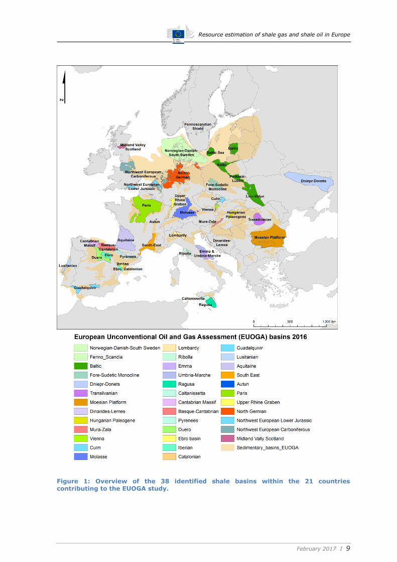
In total 38 basins (Figure 4) holding 82 formations are reviewed for this study. 49

formations from 19 countries met the requirement to undergo resource estimations.

This chapter describes the general results of each of those, per country. A detailed

overview of the calculation parameters and sensitivities per formation and basin can

be found in Appendix A.

Figure 4: Overview of all 38 EU basins identified within the EUOGA project. Of the 82 formations studied 49 were considered for of shale hydrocarbons.

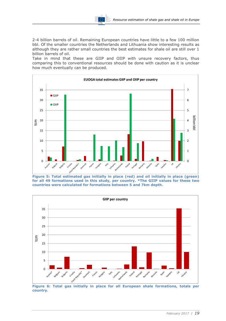
Final results of the GIIP and OIIP calculations are shown in Figure 5-9 and Table 4 and

Table 5. Total resource estimation is a P50 of 89.2 tcm of shale gas and 31.4 billion

barrels of shale oil. Countries with the biggest expected amount of shale gas are the

United Kingdom, Poland, Romania and Ukraine in the order of 9-13 tcm for the last

three and over 30 tcm for the United Kingdom (75% of the total shale gas in the EU,

Figure 5). The other 16 assessed countries estimates show relatively little shale gas or

only shale oil present (Figure 5 and Figure 6).

For the amounts of shale oil (Figure 5 and Figure 7) there are two main players, which

are Bulgaria and Poland with each over 6 billion bbl per country. Next to this France,

Portugal, UK and Ukraine are also expected to hold high amounts of shale oil around


February 2017 I 19

2-4 billion barrels of oil. Remaining European countries have little to a few 100 million

bbl. Of the smaller countries the Netherlands and Lithuania show interesting results as

although they are rather small countries the best estimates for shale oil are still over 1

billion barrels of oil.

Take in mind that these are GIIP and OIIP with unsure recovery factors, thus

comparing this to conventional resources should be done with caution as it is unclear

how much eventually can be produced.

Figure 5: Total estimated gas initially in place (red) and oil initially in place (green) for all 49 formations used in this study, per country. *The GIIP values for these two

countries were calculated for formations between 5 and 7km depth.

Figure 6: Total gas initially in place for all European shale formations, totals per country.


February 2017 I 20

Figure 7: Total oil initially in place for all contributing European shale formations, per country. *The OIIP values for these two countries were calculated for formations between 5 and 7km depth.

When looking at the amount of shale gas and shale oil initially in place per basin

(Figure 8, see basins in Figure 3) there biggest differences occur because of different

size and different amount of formations within one basin. By far the largest amount of

shale gas in present in the Northwestern European Carboniferous basin, which is also

one of the biggest basin complexes in Europe and includes the UK and the

Netherlands. Next to that the Baltic basin (including Lithuania and Poland) and the

Moesian Platform show substantial amounts of shale oil in place.

Figure 8: Total estimates for all estimated formations in gas in place (red) and oil in place (green), per basin where the Spanish basins (T10, T22, T23, T24, T33) are grouped together. For basin and formation names see Appendix A.


February 2017 I 21

Table 4: Overview of total resources of the 49 calculated formations, summarized per country.

*The GIIP and OIIP values for these two countries were calculated for formations

between 5 and 7km depth.

** Resource estimations which are partly or fully of biogenic origin.

For three countries shale gas resources were calculated for formations deeper than

5km, Austria, Czech Republic and Denmark. In the case of Austria and the Czech

Republic these reserves are the only shale gas occurrences included in this study and

therefore included in the above overview. Denmark has additional reserves located at

depth < 5km, the calculation results for the deeper formations are not included in the

general overview and only reported in the detailed calculation overview (Appendix A)

and in Table 5 and Figure 9.


February 2017 I 22

Table 5: Overview of the total amount of GIIP of the deep (5-7km) occurrences of shale hydrocarbons within the EUOGA study.

Figure 9: Overview of total estimates of deep occurrences of shale gas for EU formations deeper than 5 km.

In Figure 10 and Figure 11 estimated resources are shown subdivided into the three

different quality classes. This is done to get a better grip on the quality of the

calculated resources. From the GIIP subdivision the figure shows that here are only a

few countries which have substantial Class 1 resources, namely Denmark, Poland and

the UK. The rest of the countries do not have such a high standard of data quality

leading to the most reliant estimates. Most of the resources are of Class 2 with 60 tcm

out of 92 tcm in total. Class 3 follows with 13.4 tcm in total, coming from mainly

eastern European countries.


February 2017 I 23

For the OIP subdivision into the three classes it is visible that there are considerable

more countries with high quality data and shale formations leading to Class 1 OIIP

resources. In total 13 billion bbl resources are ranked Class 1 out of 31 billion bbl of

the entire EUOGA OIIP estimate. When looking at total numbers Poland and Bulgaria

have the two biggest OIIP estimates with more than 6 billion barrels each, but

following Figure 11 it is visible that the estimates of Poland actually are expected to be

more precise following the quality of the data the NGS send in.

Figure 10: Overview of calculated GIIP per country subdivided per class. For the class ranking system see earlier in this report. *The resource estimates for these two countries

were calculated for formations between 5 and 7km depth. **Values taken from country specific report.

Figure 11: Overview of estimated OIIP per country divided per class. The shale ranking system is explained earlier in this report.


February 2017 I 24

Comparison with existing European Resource assessments

Large scale resource assessments were published for Europe in general by the EIA

(2011 and 2013) and USGS (2010) as well as for individual countries (e.g., UK,

Andrews et al. 2013 and 2014, and Poland, PGI, 2012; see report T3 for a complete

list). In this section the results of this report are compared with the already published

reports for the individual countries.

In order to compare the results in general, it is important to compare similar reserves.

The main result of this study is the GIIP/OIIP and no systematic upscaling to TRR was

attempted. It is therefore not possible to compare these results to the study of the

USGS, as they calculated only TRR. For completeness the calculated TRR of Poland are

included in the overview.

Figure 12: Comparison of the assessment results of total gas initially in place (GIIP) of this study to earlier published results from the EIA, 2013 assessment and assessment results reported by the National Geological Surveys (see report T3). *Hungary; reported values for the Kössen Marl only, Italy; the Ribolla Basin was not

calculated in this study, Poland; total recoverable resources for the EIA values, Romania; only the Silurian of the Moesian Platform are calculated.

The study of the EIA (2013) gives an overview of the European countries with the

biggest expected shale gas and oil potential. They did not use a stochastic method for

the calculation of their values; the given value lacks therefore an uncertainty range.

When comparing their results with the results of this study, their GIIP values are

either higher or lower, but most of the time within the calculated possible range given

in this study (Figure 12). A significant exception is the UK, where the EIA identified

significantly less potential GIIP. The same observation can be made for the calculated


February 2017 I 25

OIIP with in this case the exception of France, the Netherlands and Poland, where the

EIA reports significantly higher volumes of OIIP (Figure 13). It is worth noting that the

EIA reports substantial amount of GIIP for France, where this study only shows an

OIIP. This study uses GIS data on the maturity of the French formations where

everthing lower than 450 Tmax is classified as oil mature. As the maturity data

originates directly from the NGS we have reason to believe this has led to an accurate

estimation. In general the EIA estimates are within the EUOGA ranges, but

overestimate a few countries.

The assessments of the individual countries as reported by the NGS show a similar

trend (Figure 12). The results are in most cases similar to the results of this study or

at least in the same range. Here the assessment of Romania shows the most

significant difference. They report more than 3 times as much potential gas for the

Silurian of the Moesian Platform only. Not many NGS have reported OIIP assessments.

The assessments of Hungary and the UK are in the same range as this study while the

assessment of Lithuania is significantly higher (Figure 13).

Figure 13: Comparison of the assessment results of total oil initially in place (OIIP) of

this study to earlier published results from the EIA, 2013 assessment and assessment results reported by the National Geological Surveys (see report T3). *Hungary; reported values for the Kössen Marl only, Italy; the Ribolla Basin was not calculated in this study, Poland; total recoverable resources for the EIA values, Romania; only the Silurian of the Moesian Platform are calculated.


February 2017 I 26

Discussion This report presents the results of a large scale regional assessment study, focusing

on the general distribution of parameters on a regional scale. The level of detail for

each of the used parameters and assumptions cannot be compared to local studies

that are focusing on single formations or regions only. All results are based on an

agreed upon a standard methodology as described in report T2b, an agreed upon set

of selection parameters (see this report) and the data as received from the respective

National Geological Surveys (see report T6b). Also this study acknowledges

uncertainties in the estimates, as opposed to know studies which do not. This has an

added value as the outcome of the resource estimation can be better evaluated.

Sensitivity Analyses

With the stochastic volumetric resource assessment of the 49 formations a sensitivity

analysis is performed to see which parameters have the most influence on the range

of GIIP/OIIP values. Here we discuss the general trends, Appendix A shows the

sensitivities per formation.

Sensitivity analyses of the Free Gas in Place calculations

Sensitivity analyses for the calculation of Free Gas (Figure 14) showed that on average

the gas saturation (36%) and the porosity (26%) have the biggest influence on the

calculated range of values. The amount of gas per volume rock is linearly proportional

to both parameters, and uncertainty in these parameters mainly controls uncertainty

in resource estimates. So far not many formations in Europe have information on the

gas saturation, this study therefore used an average value from all 20 reported values

from Europe and 10 published values from US shales to get a good range of possible

gas saturations. The porosity is in general much better known/measured (35% of

formations with reported values from the European formations) and is expected to

give a reasonable range at this point.

Figure 14: Overall average of free gas sensitivities of the 41 calculated formations which are assumed to hold gas.


February 2017 I 27

Sensitivity analyses of the Adsorbed Gas calculations

Sensitivity analyses for the calculation of adsorbed gas (Figure 15) show that there

are two main parameters controlling uncertainty. These parameters are the Langmuir

Volume with 54% and the formation thickness with 30%. This means that of the entire

range of resource estimates for one formation is for 54% caused by the range in the

Langmuir Volume and the range of formation thickness is for 30% responsible for the

spread in calculation outcome. The Langmuir volume has a large influence on the final

calculated amount of adsorbed mainly because it is the parameter with the biggest

range of reported values in the adsorbed gas calculation. Gasparik (2013) reports

measured values of 16.7 - 265 scf/ton for European samples. Wei Yu (2015) and Yu

and Sephehrnoori (2013) did measurements on U.S. shale where they obtain ranges

of 50.7 – 203 scf/ton for the Langmuir Volume. These measurements were the reason

to choose a log normal distribution for this parameter with a mean of 69 scf/ton and a

standard deviation of 34, according to the EU mean (report T6b). Another important

source of uncertainty in the calculation of the adsorbed gas is the thickness of the

formation. As in the case of the free gas calculation, calculated amount of gas are

linearly proportional to thickness.

Figure 15: Sensitivity analysis of the adsorbed gas content based on Monte Carlo

simulation of 41 formations.

Sensitivity analyses of the Oil Initial In Place calculations

The overall results of the Sensitivity analysis for the calculation of OIIP (Figure 16)

show that the most important parameter controlling the range of outcomes in the

resource estimates is the saturation (78%) with small influence of the porosity and

thickness values. As with the calculation of free gas this is because the total amount of

oil is linearly related to saturation and saturation is largely unknown thus leading to a

high uncertainty. With even less reported values (7 from European formations and 10

from U.S. analogues) the actual possible range of influential parameter is not very well

studied. However, oil saturation values reported from the US analogues show a much

smaller range than the gas saturation.


February 2017 I 28

Figure 16: Overall average sensitivity for oil calculations of all 24 shale formations which are expected to hold shale oil.

Parameters and assumptions

Area: At this stage in the assessment, the area is defined as the mapped outline of the

shale formation or in some cases the outline of the basin. It does not necessarily

represent the outline of the actual prospective areas of the shale formation and area is

therefore most probably overestimated in the calculations. This was addressed in this

methodology by introducing uncertainties to the areal distribution. More detailed

mapping and identification of the prospective areas will reduce this uncertainty.

Depth: For several formations, especially in Spain and Italy, only rough estimates

were available with respect to the depth of the formation. More detailed mapping of

these formations will increase their chance of success significantly and reduce the

uncertainty with respect to the amount of shale gas or oil that could be present.

Thickness and TOC: The variation in reported thickness is extremely high. In several

cases formations with less than 5m in thickness but very high TOC were reported, in

other cases the thickness of the formations was more than 2km with a low average

TOC. A better assessment of the type of shale and the distribution of TOC in the

formation could lead to a better identification of the “interesting” intervals in these

thick formations while thin intervals intercalated in thick organic lean shale formations

might be considered to be producible despite the thin character of the organic rich

formation. In the current study these very thin intervals were not included in the

calculation of the GIIP/OIIP while the thick formations were assessed using net to

gross factors as agreed upon with the NGS on how large this should be. In other

words if a N/G of a certain formation can be stated at 10% in agreement with, for

instance, reported well log measurements as known with the NGS.

Maturity: The maturity of the organic material is an important factor when identifying

whether the formation is oil, condensate or gas bearing. In most cases general

minimum, maximum and average values were reported for most formations spanning

from early oil mature to gas mature. For these formations the reported area was

subdivided into two, one for the calculation of the OIIP and one for GIIP. The

subdivision was discussed with the respective NGS. In other cases only surface


February 2017 I 29

measurements of the maturity were reported in the critical parameter sheet, which

could lead to identifying a formation as immature when at depth it could be mature.

Additional information from thermal modelling or basin modelling studies can aid in

better identifying the area of the formation that is oil mature and gas mature for a

more exact subdivision.

Porosity: In most formations the porosity had the second largest influence on the

range of calculated free GIIP values and is also a source for the range of OIIP values.

Accordingly, a proper assessment of the actual porosity distribution of a formation is

of vital importance. However, only about one third of all reported formations had

available measured porosity values and in most cases it is unclear whether these

measurements are representative of the total porosity available for hydrocarbon

storage. The burial history of the formation has the largest influence on porosity.

Calibrating modelled compaction curves to locally measured porosity values can give a

more detailed view on the porosity distribution of a formation and can therefore

reduce the uncertainty related to this parameter significantly.

Expansion factor (Reservoir pressure and temperature and gas density): The

expansion factor in the present study is calculated using an ideal gas equation

approach and, when available, the average reservoir pressure and temperature. It is

generally measured during production testing in conventional oil and gas exploration

and production. A better understanding of the distribution of the reservoir pressure

and temperature as well as the composition and density of the gas, or ideally, actual

measurements on the gas produced from the shale would decrease the uncertainty of

this parameter significantly.

All of the above mentioned parameters can be considered to be controlled by larger

scale processes that can be defined on a basin scale. They can be refined using

general regional geological studies for the individual formations based on available

data (regional mapping, measurements on available surface and well samples, etc.).

In addition to this, additional regional studies can also lead to a better identification of

potential analogues (see for instance Zijp et al. 2015). In the current study the overall

EU averages were used for parameters that were missing when no direct analogue

(data from the same formation from neighbouring country) was available. More

regional data and sample measurements could be used to update average parameter

values, and better link formations to analogues for different types of shale formation.

The parameters mentioned below are controlled by small scale processes that can

vary significantly over small distances. They have the largest impact on the

uncertainty of the calculated GIIP/OIIP. Refinement of these parameters needs

detailed local studies for individual plays and exploratory drilling.

Saturation: The gas or oil saturation has the largest impact on the uncertainty of the

calculated free GIIP/OIIP numbers. However, as previously mentioned, this parameter

cannot be estimated on a basin scale, as it is dependent on a multitude of small scale

processes and can vary significantly even within one basin. Reducing the uncertainty

of this parameter is therefore not possible in the context of a large scale regional

study, but could be done by exploratory drilling.

Langmuir pressure and volume: The Langmuir volume has the biggest impact on the

uncertainty of the adsorbed GIIP calculation. Recent measurements (e.g., Gasparik et

al. 2013, Ter Heege pers. com.) show that this parameters depends on a wide variety

of factors such as minerology or type and maturity of the organic matter. There are

therefore a large number of factors and processes that influence this parameter on a


February 2017 I 30

very small scale. This parameter is so far one of least reported for the European shale

plays.

Fraccability/Producibility (e.g., mineralogy, fracturing tests): The fraccability or

producibility is not a measurable parameter but rather a combination of factors such

as the brittleness of the shale and its permeability. In this study it was only

qualitatively addressed by looking at the reported average mineralogical composition

or in rare cases the results of fracturing tests. It does not influence the calculation of

the GIIP/OIIP but is important for the calculation of the TRR.

Cross-correlation of Monte Carlo parameters Several of the parameters used for the calculation of the GIIP/OIIP values are linked

to each other, such as depth and porosity or pressure and expansion factor. Including

these dependencies in the calculations would reduce the range of resulting values.

However, dependencies were not taken into account. For many of these relationships

basin or even play specific relationships need to be defined as they can vary

significantly even within one formation. For this regional assessment it was therefore

decided not to include the dependencies of parameters. Future studies with a more

local focus can explore dependencies and assess their effect on narrowing the range of

GIIP/OIIP values.

Recommendations

Reduction of uncertainties on a regional scale

Several shale gas formations are still underexplored with respect to several important

parameters such as depth, thickness, nett to gross, TOC reservoir temperature. Most

of these parameters can be determined using standard conventional oil and gas

exploration or production information or other types of vintage or surface data. This

type of information gathering helps to increase the general chance of success of a play

but also to narrow the uncertainty ranges of the calculation. Additional geological data

can also aid in a more detailed subdivision into assessment units and the better

definition of analogues. All newly gathered information can easily be run through the

described methodology, making frequent updates of the presented GIIP/OIIP values

possible.

Local variations of the parameters

The most influential parameters during the calculation of the GIIP/OIIP are the gas or

oil saturation and the Langmuir volume. Experience from conventional oil and gas

production as well as from shale gas/oil production in the US shows that both of these

parameters are difficult to estimate on a basin scale and can vary significantly on a

small (cm-m) scale. These parameters are usually determined in later stages of

exploration and production activities and are only meaningful on a local scale.

Activities related to the gathering of additional information on saturation and Langmuir

parameters should be focussed on areas with actual ongoing exploration activities

(e.g. Poland and the UK).

Potential technical recovery based on the notional development description

As described in report T2, upscaling to TRR using a notional development plan is

extremely dependent on the local surface and geological situation of the respective

area. It is not feasible to attach a general parameter for the upscaling. It is therefore

recommended to focus this type of research on areas with actual ongoing exploration

activities to get a realistic appraisal of the TRR.


February 2017 I 31

Conclusions

There is more than abundant evidence for large volumes of shale resources present in

the European subsurface. Out of a total of 81 shale formations from 21 countries 49

formations have been assessed. 15 formations suggest to contain both shale oil and

gas, 26 are expected to contain only shale gas and 8 are expected to contain only

shale oil all on the basis of the current screening parameters. Total volumes reach

89.2 trillion cubic meter of shale gas (P50 estimation) and 31.4 billion barrel of shale

oil (P50 estimation).

Countries with the biggest expected amount of shale gas are the United Kingdom,

Poland, Romania and Ukraine in the order of 9-13 trillion cubic meters for the last

three and over 30 tcm for the United Kingdom (75% of the total expected shale gas

resources in the EU).

The other assessed countries are expected to have very little shale gas present (e.g.,

Croatia, Czech Republic, Italy, Slovenia) or in the order of a few tcm (e.g., Bulgaria,

Denmark, Netherlands and Spain).

Highest resources in terms of shale oil initially in place are Poland, Bulgaria, the United

Kingdom, Ukraine and France in the order of 2-6.5 billion barrels of oil. Besides these

countries the other European contributing members have no to a few 100 million bbl.

According to the sensitivity analysis performed during the Monte Carlo simulation for

this study the parameters that have the highest influence on the calculation are the

saturation and the porosity for the amount of free gas, the Langmuir’s Volume and

formation thickness for the amount of adsorbed gas and the saturation for the oil in

place.

When comparing to the EIA 2013 study we see that the those estimates fall within the

calculated EUOGA ranges, where the EIA overestimates France, the Netherlands and

Poland and underestimates the UK.


February 2017 I 32

References

Advanced Resources International (ARI), (2011) world shale gas resources: an initial

assessment of 14 regions outside the United States. Washington, DC: Advanced

Resources International Inc.

Andrews, I.J. (2013) The Carboniferous Bowland Shale gas study: geology and

resource estimation. British Geological Survey for Department of Energy and Climate

Change, London, UK

Andrews, I.J. 2014. The Jurassic shales of the Weald Basin: geology and shale oil and

shale gas resource estimation. British Geological Survey for Department of Energy and

Climate Change, London, UK.

Andrews, I.J. 2013. The Carboniferous Bowland Shale gas study: geology and

resource estimation. British Geological Survey for Department of Energy and Climate

Change, London, UK

BGR (2012) Abschätzung des Erdgaspotenzials aus dichten Tongesteinen (Schiefergas)

in Deutschland. Bundesanstalt für Geowissenschaften und Rohstoffe, Hannover.

http://www.bgr.bund.de/DE/Themen/Energie/Downloads/BGR_Schiefergaspotenzial_i

n_Deutschland_2012.pdf?__blob=publicationFile (Last accessed 4 October 2016)

Cheng, K., Wu, W., Holditch, S.A. et al. 2010. Assessment of the Distribution of

Technically Recoverable Resources in North American Basins. Paper SPE 137599

presented at the Canadian Unconventional Resources and International Petroleum

Conference, Calgary, Alberta, Canada, 19-21 October

Ladage, S. et al. (2016) Schieferöl und Schiefergas in Deutschland – Potentiale und

Umweltaspekte. Bundesanstalt für Geowissenschaften und Rohstoffe (BGR), Hannover.

(http://www.bgr.bund.de/DE/Themen/Energie/Downloads/Abschlussbericht_13MB_Sc

hieferoelgaspotenzial_Deutschland_2016.html)

M.E. Curtis, B.J. Cardott, C.H. Sondergeld, C.S. Rai. Development of organic porosity

in the Woodford Shale with increasing thermal maturity. Int. J. Coal Geol., 103

(2012), pp. 26–31

DECC. 2010a. The unconventional hydrocarbon resources of Britain’s onshore basins -

shale gas. DECC Promote website, December 2010.

https://www.gov.uk/government/uploads/system/uploads/attachment_data/file/6617

2/uk-onshore-shalegas.pdf

IEA (2012) Golden rules for a golden age of gas. World energy outlook special report

on unconventional gas, p. 150. <http://www.worldenergyoutlook.org/media/

weowebsite/2012/goldenrules/WEO2012_GoldenRulesReport.pdf>.

EIA (2013) Technically recoverable shale oil and shale gas resources: An assessment

of 137 shale formations in 41 countries outside the United States. U.S. Energy

Information Administration, Washington D.C., 730 p.

http://www.eia.gov/analysis/studies/worldshalegas/. Last Accessed 5 August 2015.

Feast, G., Wu, K., Walton, J., Cheng, Z.F. and Chen, B. (2015) Modeling and

Simulation of Natural Gas Production from Unconventional Shale Reservoirs.


February 2017 I 33

International Journal of Clean Coal and Energy, 4, 23-32.

http://dx.doi.org/10.4236/ijcce.2015.42003

Gasparik, M., P. Bertier, Y. Gensterblum, A. Ghanizadeh, B. M. Krooss, R. Littke,

Geological controls on the methane storage capacity in organic-rich shales,

International Journal of Coal Geology, Volume 123, 1 March 2013, Pages 34-51, ISSN

0166-5162, http://dx.doi.org/10.1016/j.coal.2013.06.010.

Lewis, R., D. Ingraham, M. Pearcy, J. Williamson, W. Sawyer, J. Frantz, 2004, New

evaluation techniques for gas shale reservoirs, Schlumberger Reservoir Symposium

2004, Schlumberger

Monaghan, A.A. 2014. The Carboniferous shales of the Midland Valley of Scotland:

geology and resource estimation. British Geological Survey for Department of Energy

and Climate Change, London, UK.

PGI (2012) Assessment of shale gas and shale oil resources of the Lower Paleozoic

Baltic-Podlasie-Lublin basin in Poland. Resource document. Polish Geological Institute.

http://www.pgi.gov.pl/en/mineral-resources-en/shale-gas/4744-shale-

gasestimates.html. Last Accessed 5 August 2015.

Charoensuppanimit, P., Sayeed A. Mohammad, and Khaled A. M. Gasem,

Measurements and Modeling of Gas Adsorption on Shales. Energy & Fuels 2016 30

(3), 2309-2319 DOI: 10.1021/acs.energyfuels.5b02751

Chareonsuppanimit, P., S.A. Mohammad, R.L. Robinson Jr., K.A.M. Gasem. High-

pressure adsorption of gases on shales: measurements and modeling. Int. J. Coal

Geol., 95 (2012), pp. 34–46

De Silva, P.N.K., S.J.R. Simons, P. Stevens, L.M. Philip, A comparison of North

American shale plays with emerging non-marine shale plays in Australia, Marine and

Petroleum Geology, Volume 67, November 2015, Pages 16-29, ISSN 0264-8172,

http://dx.doi.org/10.1016/j.marpetgeo.2015.04.011.

Ter Heege, J., Zijp, M., Nelskamp, S., Douma, L., Verreussel, R., Ten Veen, J., De

Bruin, G., Peters, R. 2015. Sweet spot identification in underexplored shales using

multidisciplinary reservoir characterization and key performance indicators: Example

of the Posidonia Shale Formation in the Netherlands. Journal of Natural Gas Science

and Engineering

TNO (2009) Inventory non-conventional gas. TNO report TNO-034-UT-2009-00774/B,

https://www.ebn.nl/wp-content/uploads/2014/11/200909_Inventory_non-

conventional_gas.pdf (last accessed 4 October 2016)

U.S. Energy Information Administration, World Shale Gas Resources: An Initial

Assessment of 14 Regions Outside the United States, April 2011

Van Bergen, F., Zijp, M., Nelskamp, S., Kombrink, H. 2013. Shale Gas Evaluation of

the Early Jurassic Posidonia Shale Formation and the Carboniferous Epen Formation in

the Netherlands. In: Chatellier, J., Jarvie, D. (eds) Critical assessment of shale

resource plays. AAPG Memoir 103, 1–24.

Yu, W., Sepehrnoori, K., & Patzek, T. W. (2016, April 1). Modeling Gas Adsorption in

Marcellus Shale With Langmuir and BET Isotherms. Society of Petroleum Engineers.

doi:10.2118/170801-PA


February 2017 I 34

Zijp, M.H.A.A., J. ten Veen, R. Verreussel, J. ter Heege, D. Ventra, J. Martin. Shale

Gas Formation Research: from Well Logs to Outcrop – and Back Again, First Break vol.

33, February 2015

Date post:	29-Jan-2020
Category:	Documents
Upload:	others
View:	2 times
Download:	0 times

European Unconventional Oil and Gas Assessment (EUOGA) · shale gas and shale oil in Europe,...

Documents