28

Evolutionary Algorithms for Constrained Engineering Problems
Zbigniew Michalewicz,�Dipankar Dasgupta,y Rodolphe G. Le Riche,z and Marc Schoenauerx
Abstract
Evolutionary computation techniques have been receiving increasing attention regarding their potentialas optimization techniques for complex problems. Recently these techniques were applied in the areaof industrial engineering; the most-known applications include scheduling and sequencing in manufac-turing systems, computer-aided design, facility layout and location problems, distribution and trans-portation problems, and many others.
Industrial engineering problems usually are quite hard to solve due to a high complexity of theobjective functions and a signi�cant number of problem-speci�c constraints; often an algorithm tosolve such problem requires incorporation of some heuristic methods.
In this paper we concentrate on constraint handling heuristics for evolutionary computation tech-niques. This general discussion is followed by three test case studies: truss structure optimizationproblem, design of a composite laminated plate, and the unit commitment problem. These are typicalhighly constrained engineering problems and the methods discussed here are directly transferrable toindustrial engineering problems.
1 Introduction
Evolutionary computation techniques have drawn much attention as optimization methods in the lasttwo decades [33, 39, 16]. Evolutionary computation algorithms are stochastic optimization methods;they are conveniently presented using the metaphor of natural evolution: a randomly initialized pop-ulation of individuals (set of points of the search space at hand) evolves following a crude parody ofthe Darwinian principle of the survival of the �ttest. New individuals are generated using simulatedgenetic operations such as mutation and crossover. The probability of survival of the newly generatedsolutions depends on their �tness (how well they perform with respect to the optimization problemat hand): the best are kept with a high probability, the worst are rapidly discarded. Three main
� Dept. of Computer Science, University of North Carolina, Charlotte, NC 28223, USA; e-mail: [email protected]
and Institute of Computer Science, Polish Academy of Sciences, ul. Ordona 21, 01-237 Warsaw, Poland; e-mail:
[email protected] Department of Mathematics and Computer Science, University of Missouri, St. Louis, MO 63121, USA; e-mail:
[email protected] Universit�e de Technologie de Compi�egne, LG2mS Laboratory, Division MNM, Compi�egne 60200, France; e-mail:
[email protected] Polytechnique, CNRS{CMAP, Palaiseau 91128, France; e-mail: [email protected].

algorithmic trends are based on such an evolutionary scheme: Genetic Algorithms (GA) [24, 18],Evolutionary Strategies (ES) [54, 1] and Evolutionary Programming (EP) [15, 16].
From the optimization point of view, one of the main advantages of evolutionary computationtechniques is that they do not have much mathematical requirements about the optimization prob-lem. They are 0{order methods (all they need is an evaluation of the objective function), they canhandle nonlinear problems, de�ned on discrete, continuous or mixed search spaces, unconstrainedor constrained. Moreover, the ergodicity of the evolution operators makes them global in scope (inprobability).
Many industrial engineering activities involve unstructured, real-life problems that are hard tomodel, since they require inclusion of unusual factors (from accident risk factors to esthetics). Otherindustrial engineering problems are complex in nature: job shop scheduling, timetabling, travelingsalesman or facility layout problems are examples of NP-complete problems. In both cases, evolu-tionary computation techniques represent a potential source of actual breakthroughs. Their abilityto provide many near-optimal solutions at the end of an optimization run enables to choose the bestsolution afterwards, according to criteria that were either inarticulate from the expert, or badly mod-eled. Evolutionary algorithms can be made e�cient because they are exible, and relatively easy tohybridize with domain-dependent heuristics. Those features of evolutionary computation have alreadybeen acknowledged in the �eld of industrial engineering, and many applications have been reported(see, for example, [18, 47, 57]).
A vast majority of industrial engineering optimization problems are constrained problems. Thepresence of constraints signi�cantly a�ects the performance of any optimization algorithm, includingevolutionary search methods [34]. This paper focuses on the issue of constraints handling in evolution-ary computation techniques. The general way of dealing with constraints | whatever the optimizationmethod | is by penalizing infeasible points. However, there are no guidelines on designing penaltyfunctions. Some suggestions for evolutionary algorithms are given in [50], but they do not general-ize. Other techniques that can be used to handle constraints in evolutionary computation techniquesare more or less problem dependent. For instance, the knowledge about linear constraints can beincorporated into speci�c operators [37], or a repair operator can be designed that projects infeasiblepoints onto feasible ones [42]; Section 2 provides a general overview of constraints-handling methodsfor evolutionary computation techniques. Each of the next three sections presents a speci�c case studyof both an engineering constrained optimization problem and a constraint handling algorithm for evo-lutionary algorithms. Section 3 introduces a truss structure optimization problem, for which resultsare obtained using a constraint handling method based on an evolutionary sampling of the feasibleregion; Section 4 presents an evolutionary method for the design of composite laminated plate, usingthe segregated genetic algorithm, where the di�cult task of adjusting penalty parameters is avoidedby using two sub-populations, evolving according to two slightly di�erent �tness functions; Section5 is devoted to the unit commitment problem, a highly-constrained nonlinear optimization problem.Section 6 concludes the paper.
2
2 Evolutionary Computation and Constrained Optimization
In this section we discuss several methods for handling feasible and infeasible solutions in a population;most of these methods emerged quite recently. Only a few years ago Richardson et al. [50] claimed:\Attempts to apply GA's with constrained optimization problems follow two di�erent paradigms (1)modi�cation of the genetic operators; and (2) penalizing strings which fail to satisfy all the constraints."This is no longer the case as a variety of heuristics have been proposed. Even the category of penaltyfunctions consists of several methods which di�er in many important details on how the penaltyfunction is designed and applied to infeasible solutions. Other methods maintain the feasibility ofthe individuals in the population by means of specialized operators or decoders, impose a restrictionthat any feasible solution is `better' than any infeasible solution, consider constraints one at the timein a particular linear order, repair infeasible solutions, use multiobjective optimization techniques,are based on cultural algorithms (i.e., algorithms with an additional layer of beliefs which undergoesevolution as well [48]), or rate solutions using a particular co-evolutionary model (i.e., model withmore than one population, where the �tness of an individual in one population depends on the currentstate of evolution in the other population [46]).
2.1 Rejection of infeasible individuals
This \death penalty" heuristic is a popular option in many evolutionary techniques (e.g., evolutionstrategies). Note that rejection of infeasible individuals o�ers a few simpli�cations of the algorithm:for example, there is no need to evaluate infeasible solutions and to compare them with feasible ones.
The method of eliminating infeasible solutions from a population may work reasonably well whenthe feasible search space is convex and it constitutes a reasonable part of the whole search space (e.g.,evolution strategies do not allow equality constraints since with such constraints the ratio betweenthe sizes of feasible and infeasible search spaces is zero). Otherwise such an approach has seriouslimitations. For example, for many search problems where the initial population consists of infeasibleindividuals only, it might be essential to improve them (as opposed to rejecting them). Moreover,quite often the system can reach the optimum solution easier if it is possible to \cross" an infeasibleregion (especially in non-convex feasible search spaces).
2.2 Penalizing infeasible individuals
This is the most common approach in the genetic algorithms community. The domain of the objectivefunction f is extended; the approach assumes that
eval(p) = f(p)�Q(p),
where Q(p) represents either a penalty for infeasible individual p, or a cost for repairing such anindividual. The major question is, how should such a penalty function Q(p) be designed? The intuitionis simple: the penalty should be kept as low as possible, just above the limit below which infeasiblesolutions are optimal (so-called minimal penalty rule) [29]. However, it is di�cult to implement thisrule e�ectively.
3

The relationship between infeasible individual `p' and the feasible part of the search space plays asigni�cant role in penalizing such individuals: an individual might be penalized just for being infeasible,the `amount' of its infeasibility is measured to determine the penalty value, or the e�ort of `repairing'the individual might be taken into account.
Several researchers studied heuristics on design of penalty functions. Some hypotheses were for-mulated [50]:
� \penalties which are functions of the distance from feasibility are better performers than thosewhich are merely functions of the number of violated constraints,
� for a problem having few constraints, and few full solutions, penalties which are solely functionsof the number of violated constraints are not likely to �nd solutions,
� good penalty functions can be constructed from two quantities, the maximum completion costand the expected completion cost,
� penalties should be close to the expected completion cost, but should not frequently fall belowit. The more accurate the penalty, the better will be the solutions found. When penalty oftenunderestimates the completion cost, then the search may not �nd a solution."
and in [55]:
� \the genetic algorithm with a variable penalty coe�cient outperforms the �xed penalty factoralgorithm,"
where a variability of penalty coe�cient was determined by a heuristic rule.
This last observation was further investigated by Smith and Tate [56]. In their work they ex-perimented with dynamic penalties, where the penalty measure depends on the number of violatedconstraints, the best feasible objective function found, and the best objective function value found.
For numerical optimization problems,
optimize f(X), X = (x1; : : : ; xn) 2 Rn,
where
gj(X) � 0, for j = 1; : : : ; q, and hj(X) = 0, for j = q + 1; : : : ; m,
penalties usually incorporate degrees of constraint violations. Most of these methods use constraintviolation measures fj (for the j-th constraint) for the construction of the eval; these functions arede�ned as
fj(X) =
(maxf0; gj(X)g; if 1 � j � q
jhj(X)j; if q + 1 � j � m
For example, Homaifar et al. [25] assume that for every constraint we establish a family of intervalsthat determines appropriate penalty values. A similar approach is presented in Section 5 of this paper(for the unit commitment problem).
4
It is also possible (as suggested in [55] to adjust penalties in a dynamic way, taking into accountthe current state of the search or the generation number. For example, Joines and Houck [26] assumeddynamic penalties; individuals are evaluated (at the iteration t) by the following formula:
eval(X) = f(X) + (C � t)�Pm
j=1 f�j (X),
where C, � and � are constants.
Michalewicz and Attia [36] considered a method based on the idea of simulated annealing: thepenalty coe�cients are changed once in many generations (after the convergence of the algorithm toa local optima). At every iteration the algorithm considers active constraints only, the pressure oninfeasible solutions is increased due to the decreasing values of the temperature of the system.
A method of adapting penalties was developed by Bean and Hadj-Alouane [4, 20]. As the previousmethod, it uses a penalty function, however, one component of the penalty function takes a feedbackfrom the search process. Each individual is evaluated by the formula:
eval(X) = f(X) + �(t)Pm
j=1 f2j (X),
where �(t) is updated every generation t in the following way:
�(t+ 1) =
8><>:
(1=�1) � �(t); if case#1�2 � �(t); if case#2�(t); otherwise;
where cases #1 and #2 denote situations where the best individual in the last k generation was always(case #1) or was never (case #2) feasible, �1; �2 > 1, and �1 6= �2 (to avoid cycling).
Yet another approach was proposed recently by Le Riche et al. [29]. The authors designed a(segregated) genetic algorithm which uses two values of penalty parameters (for each constraint)instead of one; these two values aim at achieving a balance between heavy and moderate penalties bymaintaining two subpopulations of individuals. The population is split into two cooperating groups,where individuals in each group are evaluated using either one of the two penalty parameters. Thismethod is discussed in detail in Section 4 of this paper.
Some researchers [47, 40] reported good results of their evolutionary algorithms, which workedunder the assumption that any feasible individual was better than any infeasible one. Powell andSkolnick [47] applied this heuristic rule for the numerical optimization problems: evaluations of feasiblesolutions were mapped into the interval (�1; 1) and infeasible solutions|into the interval (1;1) (forminimization problems). Michalewicz and Xiao [40] experimented with the path planning problemand used two separate evaluation functions for feasible and infeasible individuals. The values forinfeasible solutions were increased (i.e., made less attractive) by adding such a constant, so that thebest infeasible individual was worse that the worst feasible one.
It seems that the appropriate choice of the penalty method may depend on (1) the ratio betweensizes of the feasible and the whole search space, (2) the topological properties of the feasible searchspace, (3) the type of the objective function, (4) the number of variables, (5) number of constraints,(6) types of constraints, and (7) number of active constraints at the optimum. Thus the use ofpenalty functions is not trivial and only some partial analysis of their properties is available. Also,
5

a promising direction for applying penalty functions is the use of adaptive penalties: penalty factorscan be incorporated in the chromosome structures in a similar way as some control parameters arerepresented in the structures of evolution strategies and evolutionary programming.
2.3 Maintaining feasible population by special representations and genetic oper-ators
One reasonable heuristic for dealing with the issue of feasibility is to use specialized representation andoperators to maintain the feasibility of individuals in the population. During the last decade severalspecialized systems were developed for particular optimization problems; these systems use a uniquechromosomal representations and specialized `genetic' operators which alter their composition. Someof such systems were described in [12]; other examples include Genocop for optimizing numerical func-tions with linear constraints and Genetic-2N [33] for nonlinear transportation problem. For example,Genocop assumes linear constraints only and a feasible starting point (or feasible initial population).A closed set of operators maintains feasibility of solutions. For example, when a particular componentxi of a solution vector X is mutated, the system determines its current domain dom(xi) (which is afunction of linear constraints and remaining values of the solution vector X) and the new value ofxi is taken from this domain (either with at probability distribution for uniform mutation, or otherprobability distributions for non-uniform and boundary mutations). In any case the o�spring solutionvector is always feasible. Similarly, arithmetic crossover of two feasible solution vectors X and Yyields always a feasible solution (for 0 � a � 1) in convex search spaces (the system assumes linearconstraints only which imply convexity of the feasible search space).
Often such systems are much more reliable than any other evolutionary techniques based on penaltyapproach. This is a quite popular trend: many practitioners use problem-speci�c representations andspecialized operators in building very successful evolutionary algorithms in many areas; these in-clude numerical optimization, machine learning, optimal control, cognitive modeling, classic operationresearch problems (traveling salesman problem, knapsack problems, transportation problems, assign-ment problems, bin packing, scheduling, partitioning, etc.), engineering design, system integration,iterated games, robotics, signal processing, and many others.
2.4 Repair of infeasible individuals
Repair algorithms enjoy a particular popularity in the evolutionary computation community: for manycombinatorial optimization problems (e.g., traveling salesman problem, knapsack problem, set coveringproblem, etc.) it is relatively easy to `repair' an infeasible individual. Such a repaired version can beused either for evaluation only, or it can also replace (with some probability) the original individualin the population.
The weakness of these methods is in their problem dependence. For each particular problem aspeci�c repair algorithm should be designed. Moreover, there are no standard heuristics on design ofsuch algorithms: usually it is possible to use a greedy repair, random repair, or any other heuristicwhich would guide the repair process. Also, for some problems the process of repairing infeasibleindividuals might be as complex as solving the original problem. This is the case for the nonlineartransportation problem [33], most scheduling and timetable problems, and many others.
6

On the other hand, the recently completed Genocop III system [38] for constrained numericaloptimization (nonlinear constraints) is based on repair algorithms. Genocop III incorporates theoriginal Genocop system [33] (which handles linear constraints only), but also extends it by maintainingtwo separate populations, where a development in one population in uences evaluations of individualsin the other population. The �rst population Ps consists of so-called search points which satisfylinear constraints of the problem; the feasibility (in the sense of linear constraints) of these pointsis maintained by specialized operators (as in Genocop). The second population, Pr , consists of fullyfeasible reference points. These reference points, being feasible, are evaluated directly by the objectivefunction, whereas search points are \repaired" for evaluation. The �rst results are very promising [38].
2.5 Replacement of individuals by their repaired versions
The question of replacing repaired individuals is related to so-called Lamarckian evolution, whichassumes that an individual improves during its lifetime and that the resulting improvements arecoded back into the chromosome.
Recently Orvosh and Davis [42] reported a so-called 5%-rule: this heuristic rule states that inmany combinatorial optimization problems, an evolutionary computation technique with a repairalgorithm provides the best results when 5% of repaired individuals replace their infeasible originals.In continuous domains, a new replacement rule is emerging. As mentioned earlier, the Genocop IIIsystem for constrained numerical optimization problems with nonlinear constraints is based on repairapproach. The �rst experiments (based on 10 test cases which have various numbers of variables,constraints, types of constraints, numbers of active constraints at the optimum, etc.) indicate thatthe 15% replacement rule is a clear winner: the results of the system are much better than with eitherlower or higher values of the replacement rate.
At present, it seems that the `optimal' probability of replacement is problem-dependent and itmay change over the evolution process as well. Further research is required for comparing di�erentheuristics for setting this parameter, which is of great importance for all repair-based methods.
2.6 Use of decoders
Decoders o�er an interesting option for all practitioners of evolutionary techniques. In these techniquesa chromosome \gives instructions" on how to build a feasible solution. For example, a sequence ofitems for the knapsack problem can be interpreted as: \take an item if possible"|such interpretationwould lead always to feasible solutions. However, it is important to point out that several factorsshould be taken into account while using decoders. Each decoder imposes a relationship T between afeasible solution and decoded solution.
It is important that several conditions are satis�ed: (1) for each feasible solution s there is a decodedsolution d, (2) each decoded solution d corresponds to a feasible solution s, and (3) all feasible solutionsshould be represented by the same number of decodings d. Additionally, it is reasonable to requestthat (4) the transformation T is computationally fast and (5) it has locality feature in the sense thatsmall changes in the decoded solution result in small changes in the solution itself. An interestingstudy on coding trees in genetic algorithm was reported by Palmer and Kershenbaum [45], where theabove conditions were formulated.
7
2.7 Separation of individuals and constraints
This is a general and interesting heuristic. The �rst possibility would include utilization of multi-objective optimization methods, where the objective function f and constraint violation measures fj(for m constraints) constitute a (m+ 1)-dimensional vector ~v:
~v = (f; f1; : : : ; fm).
Using some multi-objective optimization method, we can attempt to minimize its components: anideal solution x would have fj(x) = 0 for 1 � i � m and f(x) � f(y) for all feasible y (minimizationproblems). A successful implementation of similar approach was presented recently in [57].
Another approach was recently reported by Paredis [46]. The method (described in the context ofconstraint satisfaction problems) is based on a co-evolutionary model, where a population of potentialsolutions co-evolves with a population of constraints: �tter solutions satisfy more constraints, whereas�tter constraints are violated by more solutions.
Yet another heuristic is based on the idea of handling constraints in a particular order; Schoenauerand Xanthakis [52] called this method a \behavioral memory" approach. Section 3 of this paperdescribes this approach in detail.
It is also possible to incorporate the knowledge of the constraints of the problem into the belief spaceof cultural algorithms [48, 49]. The general intuition behind belief spaces is to preserve those beliefsassociated with \acceptable" behavior at the trait level (and, consequently, to prune away unacceptablebeliefs). The acceptable beliefs serve as constraints that direct the population of traits. It seems thatthe cultural algorithms may serve as a very interesting tool for numerical optimization problems, whereconstraints in uence the search in a direct way (consequently, the search in constrained spaces maybe more e�cient than in unconstrained ones!).
3 Truss Structure Optimization Problem
This section presents the problem of discrete optimization of truss structures using genetic algorithms.The original issues of this section are the constraint handling technique, based on the \behavioral mem-ory" paradigm, and the experimental comparison of the performances of GAs on both the continuousand the discrete version of the same problem.
3.1 Problem description
3.1.1 Truss structure design
Truss structure optimization is a well-known problem of structural mechanics [22]. In its simplestform, the objective structure is made of bars linking �xed nodes, and the design variables are theareas of the sections of the bars (the mechanical behavior of bars only depends on their section areas).
The objective of the optimization is to �nd the structure of minimal weight meeting some givenconstraints on the maximal displacement or/and the maximal stress under prescribed loadings.
8

1
4
35
26
1 2
3 4
5 6
7
8
9
10360’’
360’’ 360’’
x
x
x
1
3
2
1
2
3 4
8
6
10
7
5
9
2
1
8
9
4
5
6
7
12
11
1323
22
1420
18
25
16
21
1924
17
3
10
15
75’’
100’’
100’’
200’’
200’’
75’’
75’’
x
x
x
3
1
2
Figure 1: The 10-bars and 25-bars benchmark truss structures
Figure 1 shows the test cases considered in this section. Both are classical examples, used as abenchmarks for all truss structure optimization algorithms: the �rst problem is a bidimensional 10-bars truss, involving 10 design variables; in the second problem, a 3-dimensional truss is considered,made of 25 bars, but due to a priori symmetry conditions, only 7 independent variables are considered.Table 1 gives the mechanical parameters of the bars, together with the loadings considered during theoptimization.
elasticity modulus = 1:0� 104 ksidensity of material = 0:10 lb=in3
:
stress limits = �25:0 ksinumber of loadings = 1 (shown in kips)
direction of loadingloading # Node x1 x2 x3
124
0.00.0
-100.0-100.0
0.00.0
elasticity modulus = 1:0� 104 ksidensity of material = 0:10 lb=in3
:
stress limits = �40 ksinumber of loadings = 1 (shown in kips)
direction of loadingloading # Node x1 x2 x3
134
0.00.0
20.0-20.0
-5.0-5.0
Table 1: Mechanical parameters, constraints and loadings for both benchmark problems
3.1.2 The discrete problem
When the areas of the sections of the bars can take continuous values (in a prescribed interval), theproblem of truss structure optimization, as stated in the preceding subsection, can be addressed bymany deterministic optimization methods, based on gradient descent and projection operators forconstraint handling (see [14] among others). But when a mechanical engineer faces such a problem,the actual solution must be technologically feasible: the bars have to be taken from suppliers stock,and the areas of the sections can only take a �nite number of discrete values (the situation is evenworse in the case of the beam model, as only a �nite number of section shapes are available). Apossible solution is to compute the solution of the continuous problem, and to take the closest possiblevalues in the stock. But it is well-known that the discrete optimum might well be missed by such asimple strategy.
9

3.2 Constraints handling through behavioral memory
3.2.1 The behavioral memory
The \behavioral memory" paradigm, �rst introduced by De Garis [17], relies on the assumption thata population that has undergone arti�cial evolution contains more information than just the locationof the point having the highest �tness: the localization of the whole population somehow witnessesthe history of the population, how it did behave while evolving under the pressure due to the �tnessfunction at hand, hence giving indirect insight about the �tness landscape. For instance, the meandistance between individuals can be an indication of the steepness of the �tness function aroundoptimal value, giving hints on the stability of that solution. On the opposite, the existence of di�erentclusters is a sign of the multi-modality of the �tness function.
The basic idea of behavioral memory-based evolution is to use a population resulting from a �rst�tness-driven evolution as the starting point for a second evolution, using another �tness function.This second evolution is biased by the information contained in its non-random initial population.Hopefully, a good choice of the �rst �tness function can help to �nd a good optimum to the second�tness function.
A common use of such iterated scheme amounts to gradually include more and more �tness casesin the computation of the �tness (e.g., more and more test points in regression problems). It has alsobeen applied with completely di�erent successive �tness functions [17, 53]. And it can be applied tohandle constraints [52], as will be demonstrated in the following subsection.
One of the key issues for such an iterated scheme is the genetic diversity: if the population thathas evolved in the context of the �rst �tness function has converged, the bias induced by using itas a starting point for the second evolution is too strong, and this second evolution reduces to acoupling between a local search (in the small region where the population is located) and hazardousrandom search: Only a lucky mutation can help escaping the (probably local) minimum. It is ofutter importance to preserve the diversity in the population during the �rst evolution. Many schemeshave been proposed to that aim, usually in the context of multi-modal function optimization. A goodreview of these schemes can be found in [31]. The sharing scheme (see [19] for details) has been usedin this paper.
3.2.2 Iterated handling of constraints
The ideal way of handling constraints is to have the search space limited to the feasible space. In somecases, a suitable change of variables can transform the constraint problem at hand in such a desirableway [37]. But on the other hand, the main di�culty in many (deterministic) methods of constraintproblem solving is to �nd even one feasible starting point.
The basic idea underlying the behavioral memory-based constraint handling algorithm (BMCHA)is to evolve the same population using di�erent successive �tnesses to sample the feasible region, i.e.,get a population of feasible points, regardless of the objective function at hand. It is then possible touse a standard GA in the feasible region to perform the optimization task on the objective function,throwing away the infeasible points by giving them zero �tness (death penalty; see section 2.1).
10

i = 1
t = 0
% of population feasible for C ?
i = i+1
i>n ?
Random initialization of population P0
Fitness = M - C if C , ... C =0
t i
t = t+1 One GA-generation
Fitness = Objective function if C , ..., C = 0
1 i-1
0 otherwise
i
τ
1 n
Standard GA,
0 otherwise
YES
NO
NO
YES
Figure 2: Flow-chart of behavioral memory-based constraint handling algorithm
Suppose the optimization problem is the following:(max f(x); x 2 Egi(x) � 0 for i 2 [0; n]
De�ne Ci(x) = maxfgi(x); 0g; x 2 E; i 2 [0; n] and let M ti be the maximum value of Ci in the
population at generation t of step i. Figure 2 shows the ow chart of the BMCHA, which will now bedetailed.
Each one of the �rst steps of the algorithm is devoted to the satisfaction of a single constraint -while ensuring that the population remains feasible for the constraints used in the preceding steps. Sothe �tness for step i has to be a decreasing function of the violation Ci of the ith constraint. Moreover,all feasible points must have the same �tness to prevent any convergence toward a particular feasiblepoint. Finally, the maximum of these violations M t
i over the current population (t is the generationcounter) is computed, and the �tness of an individual which is feasible for the constraints 1; : : : ; i� 1is set to M t
i � Ci. Infeasible points for constraints 1; : : : ; i� 1 are assigned null �tness, and will bediscarded by the following selection step. Step i ends when a large enough part of the population(ratio � %, user-supplied parameter) is feasible for constraint i. As stated above, the sharing schemeis used throughout these �rst steps to keep the diversity of the population as large as possible.
The population after step n (the number of constraints) is then made of � % of points which are
11
feasible for the problem at hand (i.e. satisfy all constraints). The last step addresses the optimizationof the objective function f in a standard way, except that the infeasible points are discarded (seesection 2.1) by being assigned null �tness. Note the use of the sharing scheme is not necessary in thislast step.
3.3 Results
This subsection presents results obtained using the BMCHA on the truss structure optimizationproblem of section 3.1. More details can be found in [51].
3.3.1 Experimental settings
The GA used for these experiments is a home made package based on standards: stochastic remainderselection, linear �tness scaling with selective pressure of 2 [18], real encoding of the design variables,with linear cross-over [33] and ES-like Gaussian mutation [54]. In the discrete case, all oating pointnumbers are rounded to the nearest authorized value after application of the operators. One singlestep is used to handle the constraints (only constraints on the stress are considered), and the switchparameter � is set to 80%.
3.3.2 Comparative results
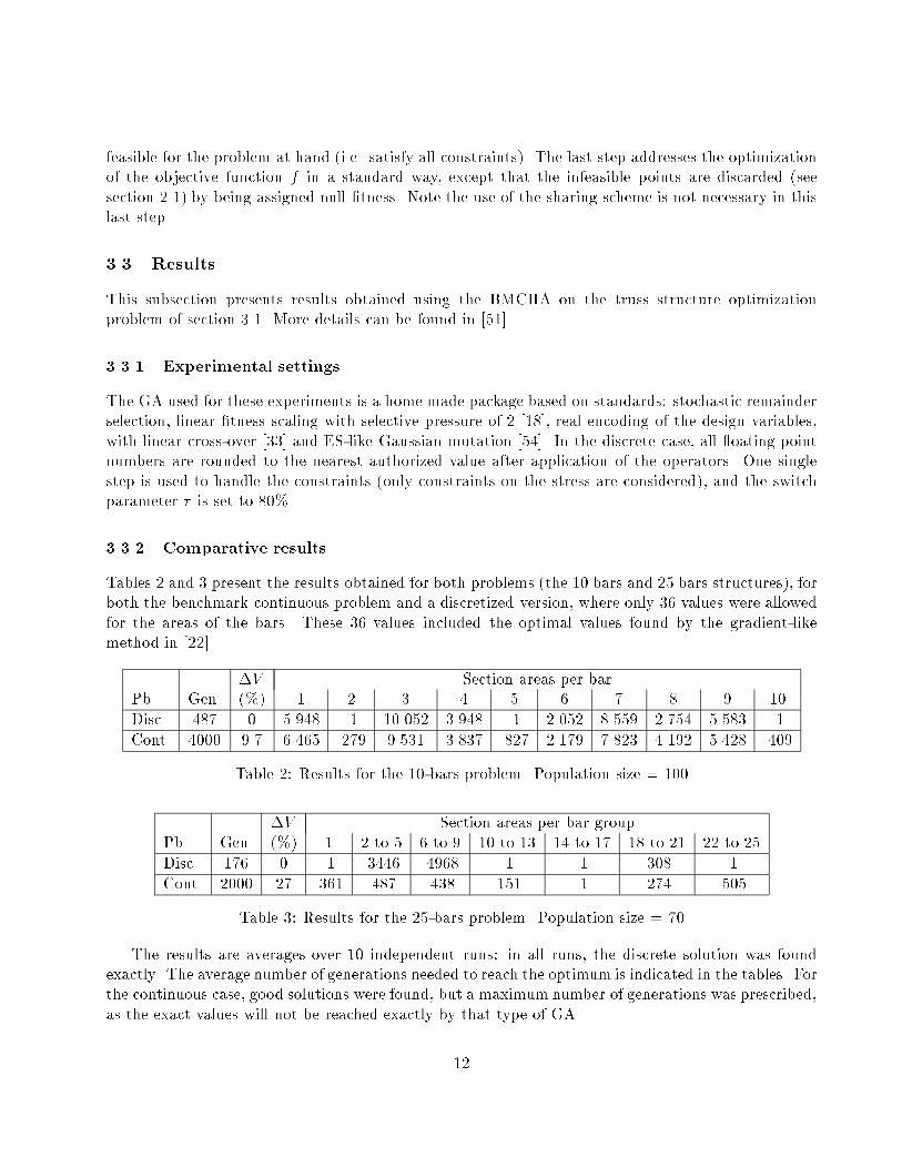
Tables 2 and 3 present the results obtained for both problems (the 10 bars and 25 bars structures), forboth the benchmark continuous problem and a discretized version, where only 36 values were allowedfor the areas of the bars. These 36 values included the optimal values found by the gradient-likemethod in [22].
�V Section areas per barPb Gen. (%) 1 2 3 4 5 6 7 8 9 10
Disc. 487 0 5.948 .1 10.052 3.948 .1 2.052 8.559 2.754 5.583 .1
Cont. 4000 9.7 6.465 .279 9.531 3.837 .827 2.179 7.823 4.192 5.428 .409
Table 2: Results for the 10-bars problem. Population size = 100
�V Section areas per bar groupPb Gen. (%) 1 2 to 5 6 to 9 10 to 13 14 to 17 18 to 21 22 to 25
Disc. 176 0 .1 .3446 .4968 .1 .1 .308 .1
Cont. 2000 27 .361 .487 .438 .151 .1 .274 .505
Table 3: Results for the 25-bars problem. Population size = 70
The results are averages over 10 independent runs: in all runs, the discrete solution was foundexactly. The average number of generations needed to reach the optimum is indicated in the tables. Forthe continuous case, good solutions were found, but a maximum number of generations was prescribed,as the exact values will not be reached exactly by that type of GA.
12
3.3.3 Discussion
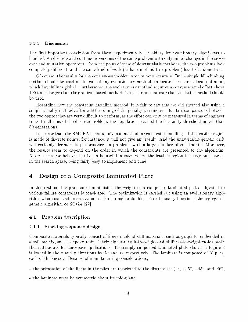
The �rst important conclusion from these experiments is the ability for evolutionary algorithms tohandle both discrete and continuous versions of the same problem with only minor changes in the cross-over and mutation operators. From the point of view of deterministic methods, the two problems lookcompletely di�erent, and the same kind of work (tailor a method to a problem) has to be done twice.
Of course, the results for the continuous problem are not very accurate. But a simple hill-climbingmethod should be used at the end of any evolutionary method, to locate the nearest local optimum,which hopefully is global. Furthermore, the evolutionary method requires a computational e�ort about100 times larger than the gradient-based method: it is clear on that case that the latter method shouldbe used.
Regarding now the constraint handling method, it is fair to say that we did succeed also using asimple penalty method, after a little tuning of the penalty parameter. But fair comparisons betweenthe two approaches are very di�cult to perform, as the e�ort can only be measured in terms of engineertime. In all runs of the discrete problem, the population reached the feasibility threshold in less than50 generations.
It is clear than the BMCHA is not a universal method for constraint handling. If the feasible regionis made of discrete points, for instance, it will not give any result. And the unavoidable genetic driftwill certainly degrade its performances in problems with a large number of constraints. Moreover,the results seem to depend on the order in which the constraints are presented to the algorithm.Nevertheless, we believe that it can be useful in cases where the feasible region is \large but sparse"in the search space, being fairly easy to implement and tune.
4 Design of a Composite Laminated Plate
In this section, the problem of minimizing the weight of a composite laminated plate subjected tovarious failure constraints is considered. The optimization is carried out using an evolutionary algo-rithm where constraints are accounted for through a double series of penalty functions, the segregatedgenetic algorithm or SGGA [29].
4.1 Problem description
4.1.1 Stacking sequence design
Composite materials typically consist of �bers made of sti� materials, such as graphite, embedded ina soft matrix, such as epoxy resin. Their high strength-to-weight and sti�ness-to-weight ratios makethem attractive for aerospace applications. The simply-supported laminated plate shown in Figure 3is loaded in the x and y directions by Xi and Yi, respectively. The laminate is composed of N plies,each of thickness t. Because of manufacturing considerations,
- the orientation of the �bers in the plies are restricted to the discrete set (0o, +45o, �45o, and 90o),
- the laminate must be symmetric about its mid-plane,
13

- the laminate must be balanced (same number of +45o and �45o layers).
Yi
Xi Xi
Yi
±459020202902
±45
=
02902±45
chromosome
E2
Figure 3: Simply supported laminated plate subjected to normal in-plane loads and coding
The objective of the optimization is to minimize the number of plies in the laminate, N , suchthat the manufacturing constraints are satis�ed, and such that the plate does not fail, neither frombuckling nor from insu�cient strength. Analytical expressions are available [28] to predict failure.Failure modes are accounted for by the constraint �cr � 1, where �cr is the critical load factor (orsafety load factor). The optimization is performed through the choice of the total number of plies andthe �ber angles for each ply, i.e., we optimize the \stacking sequence" of the laminate.
To reduce the size of the optimization problem and to automatically satisfy the balance conditionwe consider only laminates made up of 2-ply stacks 02 (two 0o plies), 902 (two 90o plies), or �45 (apair of +45o and �45o plies). The constraint on symmetry is readily implemented by considering onlyone half of the laminate (the other half being deduced by symmetry). As a result a laminate withunder N plies can be represented by a chromosome of length N=4. To accommodate variable thicknessin a �xed string length we add an empty stack and denote it as E2. Figure 3 shows an example of alaminate cross-section, and the associated coded chromosome assuming that the maximum thicknessneeded is N = 16 plies.
We minimize the objective function f which is de�ned as,
if �cr � 1; f = N + "[1� �cr];
if �cr < 1; f = N�p
cr
:(1)
The constraint on failure of the laminate is enforced by the penalty functions (1=�pcr). p is a penaltyparameters for failure. Because of the discrete nature of the problem, there may be several feasibledesigns of the same minimum thickness. Of these designs, we de�ne the optimum to be the designwith the largest failure load �cr. Therefore, the objective function is linearly reduced in proportion to
14
the failure margin for designs that satisfy the failure constraint (term "[1��cr]). A value of " (" = 6)was derived in [28] along with a more extensive analysis.
The setting of p is the subject of the present study.
4.2 The segregated genetic algorithm
4.2.1 Motivations
As it was seen in Section 2, a general approach to handling constraints in evolutionary computationtechniques is the use of penalty functions. The amount of penalty for each constraint violation istypically controlled by a penalty parameter that has a crucial in uence on the performance of thegenetic algorithm. If the amount of penalty for being infeasible is too small, the search will yieldinfeasible solutions. Reciprocally, the aw of heavily penalizing infeasible designs is that it limits theexploration of the design space to feasible regions, precluding short cuts through the infeasible domain.The general procedure is to tune the penalty functions on each problem case to assure convergencein the feasible domain while permitting an e�cient search. Apart from tuning, there is no generalsolution to the problem of optimally adjusting penalties, neither in classical numerical methods, norin evolutionary calculation. Instead of �ne tuning penalties, the segregated genetic algorithm is anattempt at desensitizing the method to the choice of penalty parameters.
4.2.2 Description
In the segregated genetic algorithm (SGGA), the population is split into two co-existing and co-operating groups that di�er in the way the �tnesses of their members are calculated. Each group usesa di�erent value of the penalty parameter p. Each of the groups corresponds to the best performingindividuals with respect to one penalty parameter. The two groups interbreed, but they are segregatedin terms of rank. Two advantages are expected. First, because the penalty parameters are di�erent,the two groups will have distinct trajectories in the design space. Because the two groups interbreed,they can help each other out of local optima. The SGGA is thus expected to be more robust than theGA. Second, in constrained optimization problems, the optimum is typically located at the boundarybetween feasible and infeasible domains. If one selects one of the penalty parameters large (say p1)and the other small (p2), one can achieve simultaneous convergence from both the feasible and theinfeasible side. The global optimum will then be rapidly encircled by the two groups of solutions, andsince the two groups of designs interbreed, the global optimum should be located faster.
For example, in structural optimization, one usually seeks to minimize the weight of a structure.The \p1 group" contains heavy designs that do not fail, while the \p2 group" contains light designsthat fail. The optimum design, which is a compromise between weight and safety, is located somewherebetween the p1 and p2 groups
Figure 4 gives the ow chart of the SGGA. Note that when the individuals are ranked, duplicatesare pushed to the bottom (low rank) of the lists. This is a protection against premature uniformizationof the population. Then, from the two lists of 2m ranked individuals, one single population of mindividuals is built which mixes the relative in uences of the two lists (this step is referred to as\merge the two lists ..." in Figure 4). One starts by selecting the best individual of the list established
15
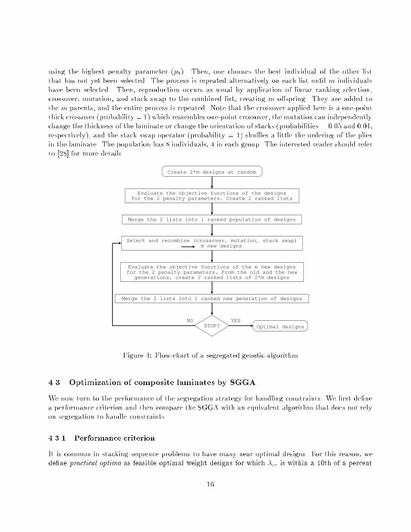
using the highest penalty parameter (p1). Then, one chooses the best individual of the other listthat has not yet been selected. The process is repeated alternatively on each list until m individualshave been selected. Then, reproduction occurs as usual by application of linear ranking selection,crossover, mutation, and stack swap to the combined list, creating m o�spring. They are added tothe m parents, and the entire process is repeated. Note that the crossover applied here is a one-pointthick crossover (probability = 1) which ressembles one-point crossover, the mutation can independentlychange the thickness of the laminate or change the orientation of stacks (probabilities = 0.05 and 0.01,respectively), and the stack swap operator (probability = 1) shu�es a little the ordering of the pliesin the laminate. The population has 8 individuals, 4 in each group. The interested reader should referto [28] for more details.
Create 2*m designs at random
Evaluate the objective functions of the designsfor the 2 penalty parameters. Create 2 ranked lists
Merge the 2 lists into 1 ranked population of designs
Select and recombine (crossover, mutation, stack swap) m new designs
Evaluate the objective functions of the m new designsfor the 2 penalty parameters. From the old and the new
generations, create 2 ranked lists of 2*m designs
Merge the 2 lists into 1 ranked new generation of designs
Optimal designsSTOP?YESNO
Figure 4: Flow-chart of a segregated genetic algorithm
4.3 Optimization of composite laminates by SGGA
We now turn to the performance of the segregation strategy for handling constraints. We �rst de�nea performance criterion and then compare the SGGA with an equivalent algorithm that does not relyon segregation to handle constraints.
4.3.1 Performance criterion
It is common in stacking sequence problems to have many near optimal designs. For this reason, wede�ne practical optima as feasible optimal weight designs for which �cr is within a 10th of a percent
16

of �cr of the global optimum. The measure of the performance of the algorithm is the reliability ofthe algorithm. It is the probability the algorithm has of �nding a practical optimum after a givennumber of analyses (evaluations of the objective function). In this study, the reliability is calculatedby averaging the results of 3000 independent searches for each implementation that is being tested.Each search is 6000 analyses long. The price of the search is the number of analyses necessary to reacha reliability of 80%.
4.3.2 Results
GA type Price of search
EGA p=0.4 r = 0:15�
EGA p=0.5 1380EGA p=5.0 3980
SGGA p1=0.5 p2=0.4 1270SGGA p1=5.0 p2=0.4 3350SGGA p1=0.5 p2=0.5 990
Table 4: Price of the search of EGA and SGGA. � : reliability at 6000 analyses. The price is notde�ned because 80% reliability was not achieved within 6000 analyses
We consider a graphite-epoxy plate with longitudinal and lateral dimensions a = 20 in. and b =5 in., respectively. The material properties are: E1 = 18.50 � 106 psi; E2 = 1.89 � 106 psi; G12 =0.93 � 106 psi; �12 = 0.3; t = 0.005 in. (t is the basic ply thickness). The maximum thickness for alaminate is assumed to be 64 plies, i.e., the string length is 64/4 = 16. Three loadings are consideredsimultaneously: [X1 = 12,000. lb/in, Y1 = 1,500. lb/in], [X2 = 10,800. lb/in, Y2 = 2,700. lb/in], [X3
= 9,000. lb/in, Y3 = 4,500. lb/in], and the ultimate allowable strains are �ua1 = 0.008, �ua2 = 0.029, ua12= 0.015. This optimization problem has been treated over 100000 times, so the best-known design istaken as the optimum.
The performance of the SGGA (p1 6= p2) is compared with the performance of the same algorithmwhen p1 = p2. When p1 = p2, the co-evolutionary aspect of the SGGA is lost to yield an algorithmthat we call superElitist Genetic Algorithm (EGA). Table 4 gives the prices of the search for EGAand SGGA. Three values of the penalty parameter p, 0.4, 0.5 and 5.0. These values were foundexperimentally. p = 0:5 is the optimal setting of the penalty parameter, as it can be seen in Table 4.p = 0:4 is a small value of the penalty parameter, and the search often gets trapped in the infeasibleregion of the design space (although the global optimum is still feasible for this value of p). p = 5:0is a large value of the penalty parameter. All three combinations of p1 and p2, p1 6= p2, are testedwith the SGGA.
Table 4 shows that EGA endures a dramatic decrease in performance if p is poorly chosen. Forp = 0:4, the reliability achieved by EGA is only 15% after 6000 analyses. This is because EGA getstrapped at a local infeasible optimum (N = 44 plies, �cr � 0.8 when the global optimum has N = 48plies, �cr � 1.01). SGGA on the contrary maintains a decent level of performance for the worstpossible choice of penalty parameters. For p1 too large (=5.0) and p2 too small (=0.4), the price of
17
SGGA is 3350 analyses. Providing that p1 is taken small and p2 large, SGGA is less sensitive to thetuning of p than EGA is.
Furthermore, segregation speeds up the search since the best price with SGGA is 990 analysesagainst 1380 analyses for EGA. Those �gures, compared to the size of the design space (416 � 4: 109),show how e�cient specialized evolutionary algorithms can be on this type of problem.
5 Unit Commitment Problem
The unit commitment in a power system is a complex optimization problem because of multiplenonlinear constraints which can not be violated while �nding the optimal schedule. An electric powernetwork usually operates under continuous variation of consumer load demand. This demand forelectricity exhibits such large variations between weekdays and weekends, and between peak and o�-peak hours that it is not economical to keep all the generating units continuously on-line; since fuelexpenses constitute a signi�cant part of the overall generation costs. In a system, there exist varioustypes of generating units that are categorized on the basis of fuel used (e.g., coal, natural gas, oil),production costs, generating capacities and operating characteristics. Thus determining which unitsshould be kept on-line and which ones should not, constitutes a di�cult decision-making task for theoperators seeking to minimize the system operational cost.
Several mathematical programming techniques have been reported in the literature [6, 32, 44] tosolve the unit commitment problem. They primarily include priority list and heuristic methods, dy-namic programming, method of local variations, mixed integer programming, lagrangian relaxation,branch and bound, bender decomposition, etc. Among these classical techniques, dynamic program-ming methods based on the priority list have been used most extensively throughout the power in-dustry. However, di�erent strategies (for selecting a set of units from priority list) have been adoptedwith dynamic programming to limit the search space and execution time.
In recent work, some researchers have suggested arti�cial intelligence based techniques to sup-plement the limitation of mathematical programming methods. These are simulated annealing [59],expert systems [41], heuristic rule-based systems [58] and neural networks [43]; these hybrid approacheshave demonstrated some improvement in solving unit commitment problems. However, heuristic andexpert system based mathematical approaches require a lot of operator interaction which is trouble-some and time-consuming [21].
This section presents an evolutionary algorithm to solve the unit commitment problem. The mainpurpose of using the evolutionary approach is to replace classical solution methods with a population-based global search procedure which has some distinct advantages.
5.1 Problem Description
The unit commitment problem involves in determining which of the generating units are to be commit-ted (on or o�) in every time interval during the scheduling time horizon. This decision must take intoaccount load forecast information and the economic implications of the startup or shutdown of variousunits. The transition between their commitment states must satisfy the operating (minimum up and
18

down time) constraints. So the demand and the reserve requirement impose global constraints in cou-pling all active generating units, while the di�erent operating characteristics of each unit constitutelocal constraints. Also some stand-by capacity (called spinning reserve) is required to be maintainedat all time in addition to the forecasted load in order to meet unexpected load demand and suddenunit failures.
5.2 Objective function
The objective of the unit commitment problem is to determine the state of each unit uti (0 or 1) ateach time period t, where unit number i = 1 : : :Umax, and time periods t = 1 : : :Tmax, so that theoverall operation cost is a minimum within the scheduling time horizon.
minPTmax
t=1
PUmax
i=1 [uti AFLCi + uti(1� ut�1i ) Si(xti) + ut�1i (1� uti) Di] (1)
For each committed unit, the cost involved is the start-up cost (Si) and the Average Full LoadCost (AFLCi) per MWh, according to the unit's maximum capacity such that
PUmax
i=1 Pimax � Rt + Lt; (2)
where Pimax is the maximum output capacity of unit i, Lt is the demand and Rt is the spinning
reserve in time period t. The above objective function should satisfy minimum up-time and down-timeconstraints of generating units.
The start-up cost is expressed as a function of the number of hours (xti) the unit has been down andthe shut-down cost is considered as a �xed amount (Di) for each unit per shut-down, and these statetransition costs are applied in the period when the unit is committed or taken o�-line respectively[23].
However, unit commitment decisions based solely on the unit-AFLC usually do not provide suf-�cient information about the impact of system load conditions on how e�ciently (e.g., fully) thecommitted units being utilized while determining a near-optimal commitment [27]. To compensatethe de�ciency associated with committed decisions based on the classical AFLC of units, an index isused to measure the utility of each commitment decision, while satisfying the global constraint (equ.(2)). This is called an utility factor and can be calculated as
Utility Factor = Load�Reserve RequirementsTotal committed output
. So during the performance evaluation, commitmentdecisions having a low utility factor are penalized accordingly.
5.3 GA-based Unit Commitment
The task of the GA-based commitment scheduler is to ensure the adequate power supply over the entirescheduling period, in a most cost-e�ective manner while satisfying the system operational constraints.For developing a GA-based scheduler, we �rst map the problem space into the framework of geneticalgorithm. Accordingly, each chromosome is encoded in binary form (bit string) to represent thestate of commitment variables for the units that are available in the system. So the allele valueat loci give the state (on/o�) of the units as a commitment decision at each time period. In thisstudy, a short-term commitment is considered with a 24-hour time horizon. Since the system load
19
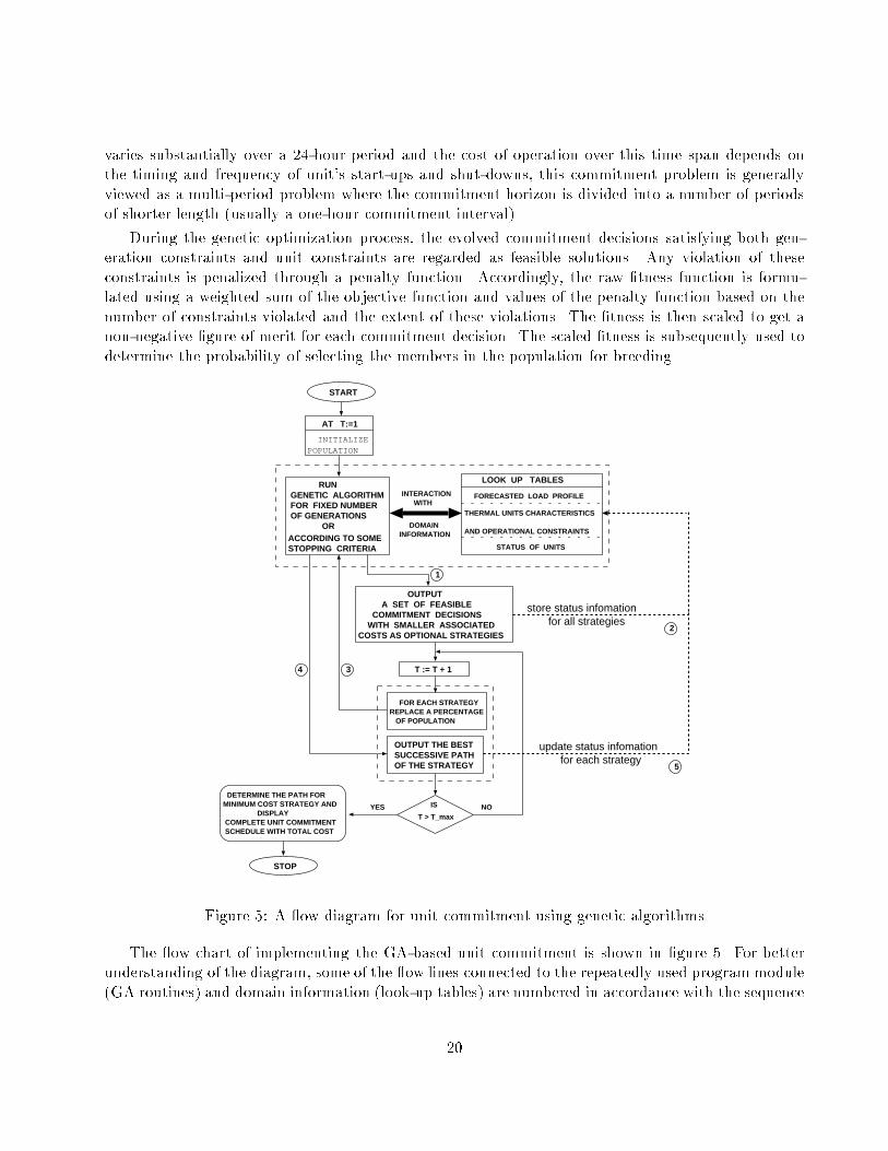
varies substantially over a 24-hour period and the cost of operation over this time span depends onthe timing and frequency of unit's start-ups and shut-downs, this commitment problem is generallyviewed as a multi-period problem where the commitment horizon is divided into a number of periodsof shorter length (usually a one-hour commitment interval).
During the genetic optimization process, the evolved commitment decisions satisfying both gen-eration constraints and unit constraints are regarded as feasible solutions. Any violation of theseconstraints is penalized through a penalty function. Accordingly, the raw �tness function is formu-lated using a weighted sum of the objective function and values of the penalty function based on thenumber of constraints violated and the extent of these violations. The �tness is then scaled to get anon-negative �gure of merit for each commitment decision. The scaled �tness is subsequently used todetermine the probability of selecting the members in the population for breeding.
START
AT T:=1
RUN GENETIC ALGORITHM FOR FIXED NUMBER OF GENERATIONS
OR
OUTPUT A SET OF FEASIBLE COMMITMENT DECISIONS WITH SMALLER ASSOCIATEDCOSTS AS OPTIONAL STRATEGIES
STOP
YES NO T > T_max
IS
T := T + 1
REPLACE A PERCENTAGE OF POPULATION
DETERMINE THE PATH FORMINIMUM COST STRATEGY AND DISPLAY COMPLETE UNIT COMMITMENT SCHEDULE WITH TOTAL COST
LOOK UP TABLES
FORECASTED LOAD PROFILE
THERMAL UNITS CHARACTERISTICS
AND OPERATIONAL CONSTRAINTS
STATUS OF UNITS
update status infomation for each strategy
INTERACTION WITH
DOMAININFORMATIONACCORDING TO SOME
STOPPING CRITERIA
FOR EACH STRATEGY
OUTPUT THE BESTSUCCESSIVE PATHOF THE STRATEGY
INITIALIZEPOPULATION
store status infomation for all strategies
1
2
34
5
Figure 5: A ow diagram for unit commitment using genetic algorithms
The ow chart of implementing the GA-based unit commitment is shown in �gure 5. For betterunderstanding of the diagram, some of the ow lines connected to the repeatedly used program module(GA routines) and domain information (look-up tables) are numbered in accordance with the sequence
20

of execution. The GA-based unit commitment program starts with a random initial population (atT=1) and computes the �tness of each individual (commitment decision) using the forecasted loaddemand at each period, and the operating constraints of the units (using lookup tables). Each timethe genetic optimizer is called, it runs for a �xed number of generations or until the best individualremains unchanged for a long time (here 100 successive generations).
Since the unit commitment problem is time-dependent, these piecewise approaches (moving win-dow) of working forward in time and retaining the best decision, can not be guaranteed to �nd theoptimal commitment schedule. The reason for this is that a decision with signi�cantly higher costsduring the early hours of scheduling could lead to signi�cant savings later and may produce a loweroverall cost commitment schedule. For �nding near-optimal solutions, a number of feasible commit-ment decisions (less than or equal to a prede�ned value S) with smaller associated costs are savedat each time period. These strategies1 determine how many possible alternative paths are availableat each period for �nding the overall operation cost. The selection of S is e�ective in economicalscheduling (in �nding an optimal solution), memory requirement and computation time. In order tosave computation time the same strategies are carried forward to the next period if the load remainsunaltered or varies slightly in the current period such that load-reserve requirements are satis�ed by allstrategies. If a strategy cannot meet the demand of present period, the genetic optimization process isperformed for the period to �nd a feasible successor paths with smaller cost. This approach increasesthe likelihood of �nding the path of minimum cumulative cost.
These temporary commitment strategies are used to update the status information of the units (up-time/down-time counter) to keep track of the units in service or shutdown for a number of successivehours. In the next time period, half of the population is replaced by randomly generated individualsto introduce diversity in the population so that the search for new commitment strategy can proceedaccording to the load demand. The purpose of keeping half of the previous population is that in mostsituations the load varies slightly in some successive time intervals and the previous better individuals(commitment strategies) are likely to perform well in the current period. However, if there is a drasticchange in load demand, newly generated individuals can explore the commitment space for �ndingthe best solution. The iterative process continues for each period in the scheduling horizon, and theaccumulated cost associated with each commitment strategy gives the overall cost for the commitmentpath.
During these multi-period optimization processes, if in a particular period no feasible solution(strategy) is found, the process is repeated so that at least one feasible solution is found beforeshifting to the next period. However, in our test example such repetitions are required only in a fewoccasions in later periods.
5.4 Experimental results
The GA-based unit commitment scheduler has been tested on a number of example cases and somewere reported in [9, 7]. Due to space restrictions we report results of one example problem whichconsists of 10 thermal units (please refer to [9] for details). It is to be noted that the capacities, costsand operating constraints varied greatly among the various generating units in this example system.
1A strategy is a sequence of commitment decisions from the starting period to the current period with its accumulated
cost.
21

Di�erent type of load pro�les are tested which represent typical operating circumstances in the studiedpower system. We have considered a short term scheduling where the time horizon is 24-hour andscheduling for an entire day is done in advance which may be repeated using load pro�le of each dayfor a long-term scheduling.
In these experiments, the spinning reserve requirement is assumed to be 10% of the expected hourlypeak load. A program implementing the algorithm has been run on a SUN (sparc 2) workstationunder UNIX 4.1.1 operating system. The experiment is conducted with a population size of 250 usingdi�erent crossover and mutation rates. For the result reported here (shown in a tabular form), acrossover probability of 78% and mutation rate of 15% were used along with a stochastic remainderselection scheme [5] for reproduction. We also used an elitist scheme which passes the best individualunaltered to the succeeding generation. Each run was allowed to continue up to 500 generations andthe strategy path with minimum cumulative cost gives a near-optimal commitment for the wholescheduling period.
For this example, Table 5 gives the characteristics and the initial states of the generating units.Table 6 gives commitment schedule for two cases, which were run independently. In �rst case, one bestsolution is saved at each time period and in second case, multiple least cost strategies are saved fordetermining the minimum cost path. A comparison shows that substantial reduction in overall costcan be achieved when the best commitment schedule is determined from multiple least cost strategies.
In this table, the second column gives the hourly load demand, the third column shows totalrequirement after adding spinning reserve, the rest columns give the total output capacity (in MW)of the committed units and the state of units in each case, where `1' is used to indicate a unit iscommitted, `0' to indicate that a unit is decommitted. The GA-based unit-commitment system havebeen tested under di�erent operating conditions in order to evaluate the algorithm's performance.
It is observed that the scheduling which produces optimal power output does not always give theoverall minimum cost scheduling, and also the minimum cost scheduling is very sensitive to the systemparameters and the operating constraints of the generating units.
5.5 Discussion
The unit commitment is a highly-constrained decision-making problem, and traditional methods makeseveral assumptions to solve the problem. Most of these traditional methods require well-de�ned per-formance indices and explicitly use unit selection list or priority order list for determining the commit-ment decisions. The major advantages of using GAs are that they can eliminate some limitations ofmathematical programming methods. Particularly, the GA-based unit commitment scheduler evalu-ates the priority of the units dynamically considering the system parameters, operating constraints andthe load pro�le at each time period while evolving near-optimal schedules. Though global optimalityis desirable, but in most practical purposes near-optimal (or good feasible) solutions are generallysu�cient. This evolutionary approach attempts to �nd the best schedule from a set of good feasiblecommitment decisions. Also the method presented in this section can include more of the constraintsthat are encountered in real-world applications of this type.
This study suggests that the GA-based method for short-term unit commitment is a feasible al-ternative approach and is easy to implement. One disadvantage of this approach is the computational
22

Unit Maximum Min. Up Min. Down Initial St Up cost Sh DownNo. Capacity Time Time Status b1 b2 b3 Cost AFLC
(MW) (hr) (hr) (hr)1 60 3 1 -1 85 20.588 0.2 15 15.32 80 3 1 -1 101 20.594 0.2 25 163 100 4 2 1 114 22.57 0.2 40 20.24 120 4 2 5 94 10.65 0.18 32 20.25 150 5 3 -7 113 18.639 0.18 29 25.66 280 5 2 3 176 27.568 0.15 42 30.57 520 8 4 -5 267 34.749 0.09 75 32.58 150 4 2 3 282 45.749 0.09 49 26.09 320 5 2 -6 187 38.617 0.130 70 25.810 200 5 2 -3 227 26.641 0.11 62 27.0
(-) indicates unit is down for hours and positive otherwise.
*We used start-up cost = b1;i(1 � e�b3;i:(xti)) + b2;i.
Table 5: Characteristics and initial state of the thermal units
--------------------------------------------------------------------------------
CASE - 1 CASE - 2
When only best strategy Best of five least
is saved at each hour cost strategies saved
--------------------------------------------------------------------------------
Time Load Load + Committed State of Committed State of
in Demand Reserve Output units Output Units
(hr) (MW) (MW) (MW) (MW)
--------------------------------------------------------------------------------
1 1459.00 1677.85 1700.00 1011111110 1710.00 1110011111
2 1372.00 1577.80 1710.00 1110111011 1860.00 1110111111
3 1299.00 1493.85 1710.00 1110111011 1550.00 1111101011
4 1280.00 1472.00 1490.00 0111101011 1490.00 0111101011
5 1271.00 1461.65 1470.00 1011101011 1470.00 1011101011
6 1314.00 1511.10 1550.00 1111101011 1550.00 1111101011
7 1372.00 1577.80 1600.00 1101101111 1580.00 1110101111
8 1314.00 1511.10 1600.00 1101101111 1520.00 0110101111
9 1271.00 1461.65 1500.00 1111101110 1500.00 1111101110
10 1242.00 1428.30 1630.00 1111011110 1500.00 1111101110
11 1197.00 1376.55 1420.00 0111011010 1380.00 1011110111
12 1182.00 1359.30 1360.00 1111011001 1360.00 1101110111
13 1154.00 1327.10 1330.00 1001111001 1360.00 1101110111
14 1138.00 1308.70 1410.00 1101111001 1310.00 1111110011
15 1124.00 1292.60 1310.00 1111110011 1310.00 1111110011
16 1095.00 1259.25 1280.00 0110110111 1260.00 1111110110
17 1066.00 1225.90 1260.00 1010110111 1260.00 1111110110
18 1037.00 1192.55 1260.00 1010110111 1200.00 0111110110
19 993.00 1141.95 1180.00 1111100111 1180.00 1111100111
20 978.00 1124.70 1200.00 1111001010 1180.00 1111100111
21 963.00 1107.45 1320.00 0101011010 1180.00 1111100111
22 1022.00 1175.30 1210.00 1101011100 1180.00 1111100111
23 1081.00 1243.15 1340.00 1110111100 1250.00 0111110011
24 1459.00 1677.85 1900.00 1011111111 1680.00 1111011011
-------------------------------------------------------------------------------
Cumulative scheduling Cumulative scheduling
cost = 940101.65 cost = 877854.32
-------------------------------------------------------------------------------
The difference in cost is approximately 7% in these two cases.
Table 6: Unit commitment schedules determined by the genetic algorithm23
time needed to evaluate the population in each generation, but since genetic algorithms can e�cientlybe implemented in a highly parallel fashion, this drawback becomes less signi�cant with its implemen-tation in a parallel machine environment. Further research should address a number of issues to solvethe commitment problem: Experiments should be carried out with large power systems having hun-dreds of units in multiple areas. One possible approach may be to use indirect encoding or use of somegrammar rule (as used in other GA applications) for representing a cluster of units in a chromosome.Also in a large power plant, the unit-commitment task may be formulated as a multi-objective con-strined optimization problem; where it is necessary to take into account not only the operational costbut also the emission of pollutant and other environmental factors as mutually con icting objectives.Finally, it may be also possible to integrate both the unit commitment and the economic dispatch (i.e.the optimal allocation of the load among the committed units) in a single evolutionary optimizationframework using our recently-developed structured genetic model [8].
6 Conclusions
The paper surveys many heuristics which support the most important step of any evolutionary tech-nique: evaluation of the population. It is clear that further studies in this area are necessary: di�erentproblems require di�erent \treatment". It is also possible to mix di�erent strategies described in thispaper. The authors are not aware of any results which provide heuristics on relationships betweencategories of optimization problems and evaluation techniques in the presence of infeasible individuals;this is an important area of future research.
References
[1] B�ack, T., Evolutionary Algorithms in Theory and Practice, New-York, Oxford University Press,1995.
[2] Baptistella, L.F.B. and Geromel, J.C., A Decomposition Approach to Problem of Unit Commit-ment Schedule for Hydrothermal Systems, IEE Proceedings { Part C, Vol.127, Np.6, pp.250{258,November 1980.
[3] Bard, J.F., Short-Term Scheduling of Thermal-Electric Generators using Lagrangian Relaxation,Operations Research, Vol.36, No.5, pp.756{766, Sept/Oct. 1988.
[4] Bean, J.C. and Hadj-Alouane, A.B., A Dual Genetic Algorithm for Bounded Integer Programs,Department of Industrial and Operations Engineering, The University of Michigan, TR 92-53,1992.
[5] Booker, L.B., Intelligent Behavior as an Adaptation to the Task Environment, PhD thesis, Com-puter Science, University of Michigan, Ann Arbor, 1982.
[6] Cohen, A.I. and Yoshimura, M., A Branch-and-Bound Algorithm for Unit Commitment, IEEETransactions on Power Apparatus and Systems, Vol.102, No.2, pp.444{449, February 1983.
24

[7] Dasgupta, D., Unit Commitment in Thermal Power Generation using Genetic Algorithms, SixthInternational Conference on Industrial & Engineering Applications of Arti�cial Intelligence andExpert Systems (IEA/AIE), 1993, pp.374{383.
[8] Dasgupta, D., Structured Genetic Algorithms in Search and Optimization, Ph.D. Thesis, Dept. ofComputer Science, University of Strathclyde, Glasgow, UK, 1993.
[9] Dasgupta, D., and McGregor, D.R., Thermal Unit Commitment using Genetic Algorithms, IEEProceedings { Part C: Generation, Transmission and Distribution, Vol.141, No.5, September 1994,pp.459{465.
[10] Dasgupta, D., and McGregor, D.R., Short-Term Unit Commitment using Genetic Algorithms,Proceedings of 5th IEEE International Conference on Tools with Arti�cial Intelligence (TAI'93),November 8{11, 1993, Boston, USA, pp.240{247.
[11] Davidor, Y., Epistasis Variance: Suitability of a Representation to Genetic Algorithms, ComplexSystems, Vol.4, pp.369{383, 1990.
[12] Davis, L., Handbook of Genetic Algorithms, New York, Van Nostrand Reinhold, 1991.
[13] Eshelman, L.J. and Scha�er, J.D, Real-Coded Genetic Algorithms and Interval Schemata, Foun-dations of Genetic Algorithms { 2, Morgan Kaufmann, Los Altos, CA, 1993, pp.187{202.
[14] Fletcher, R., Practical Methods of Optimization, second edition, John Wiley & Sons, 1987.
[15] Fogel, L. J., Owens, A. J. and Walsh M. J., Arti�cial Intelligence through Simulated Evolution,New York, John Wiley, 1966.
[16] Fogel, D. B., Evolutionary Computation. Toward a New Philosophy of Machine Intelligence, IEEEPress, 1995.
[17] de Garis, H., Genetic Programming: Building Arti�cial Nervous Systems using Genetically Pro-grammed Neural Networks Modules, Proceedings of the 7th International Conference on MachineLearning, R. Porter and B. Mooney (Eds), Morgan Kaufmann, pp.132{139, 1990.
[18] Goldberg, D.E., Genetic Algorithms in Search, Optimization and Machine Learning, Addison-Wesley, Reading, MA, 1989.
[19] Goldberg D. E. and Richardson, J, Genetic Algorithms with Sharing for Multi-Modal FunctionOptimization, Proceedings of the Second ICGA, Lawrence Erlbaum Associates, pp.41{49, 1987.
[20] Hadj-Alouane, A.B. and Bean, J.C., A Genetic Algorithm for the Multiple-Choice Integer Pro-gram, Department of Industrial and Operations Engineering, The University of Michigan, TR92-50, 1992.
[21] Hamdam, A.R. and Mohamed-Nor, K., Integrating an Expert System into a Thermal Unit-Commitment Algorithm, IEE Proceedings { Part C, Vol.138, No.6, pp.553{559, November 1991.
[22] Haug, E.J. and Arrora, J.S., Applied Optimal Design, John Wiley and Sons, Inc., New York,1979.
25

[23] Hobbs, W.J., Hermon, G., Warner, S., and Sheble, G.B., An Advanced Dynamic ProgrammingApproach for Unit Commitment, IEEE Transactions on Power Systems, Vol.3, No.3, pp.1201{1205, August 1988.
[24] Holland, J., Adaptation in Natural and Arti�cial Systems, University of Michigan Press, AnnHarbor, 1975.
[25] Homaifar, A., Lai, S. H.-Y., Qi, X., Constrained Optimization via Genetic Algorithms, Simulation,Vol.62, No.4, 1994, pp.242{254.
[26] Joines, J.A. and Houck, C.R., On the Use of Non-Stationary Penalty Functions to Solve NonlinearConstrained Optimization Problems With GAs, Proceedings of the First IEEE ICEC 1994, pp.579{584.
[27] Lee, F.N., The Application of Commitment Utilization Factor (CUF) to Thermal Unit Commit-ment, IEEE Transactions on Power Systems, Vol.6, No.2, pp.691{698, May 1991.
[28] Le Riche, R., and Haftka, R.T., Improved Genetic Algorithm for Minimum Thickness CompositeLaminate Design, Composites Engineering, Vol.3, No.1, pp. 121-139, 1995.
[29] Le Riche, R., Knopf-Lenoir, C., and Haftka, R.T., A Segregated Genetic Algorithm for ConstrainedStructural Optimization, Proceedings of the Sixth ICGA, Morgan Kaufmann, pp.558{565, 1995.
[30] Lowery, P.G., Generating Unit Commitment by Dynamic Programming, IEEE Transactions onPower Apparatus and Systems, Vol.85, No.5, pp.422{426, May 1966.
[31] Mahfoud, S.W., A Comparison of Parallel and Sequential Niching Methods, Proceedings of theSixth ICGA, Morgan Kaufmann, pp.136{143, 1995.
[32] Merlin, A. and Sandrin, P., A New Method for Unit Commitment at Electricite De France, IEEETransactions on Power Apparatus and Systems, Vol.102, No.5, pp.1218{1225, May 1983.
[33] Michalewicz, Z., Genetic Algorithms + Data Structures = Evolution Programs, Springer-Verlag,New York, 2nd edition, 1994.
[34] Michalewicz, Z.,A Survey of Constraint Handling Techniques in Evolutionary Computation Meth-ods, Proceedings of the 4th Annual Conference on EP, MIT Press, Cambridge, MA, pp.135{155,1995.
[35] Michalewicz, Z., Genetic Algorithms, Numerical Optimization, and Constraints, Proceedings ofthe Sixth ICGA, Morgan Kaufmann, pp.151{158, 1995.
[36] Michalewicz, Z., and Attia, N., Evolutionary Optimization of Constrained Problems, Proceedingsof the 3rd Annual Conference on EP, World Scienti�c, 1994, pp.98{108.
[37] Michalewicz, Z. and Janikow, C., Handling Constraints in Genetic Algorithms, Proceedings ofthe Fourth ICGA, Morgan Kaufmann, 1991, pp.151{157.
26

[38] Michalewicz, Z. and Nazhiyath, G., Genocop III: A Co-evolutionary Algorithm for NumericalOptimization Problems with Nonlinear Constraints, Proceedings of the Second IEEE ICEC, Perth,Australia, 29 November { 1 December 1995.
[39] Michalewicz, Z., Scha�er, J. D., Schwefel, H.-P., Fogel, D. B. and Kitano, H., Eds, Proceedingsof the First IEEE International Conference on Evolutionary Computation, Orlando, June 1994,IEEE Press.
[40] Michalewicz, Z. and Xiao, J., Evaluation of Paths in Evolutionary Planner/Navigator, Proceed-ings of the 1995 International Workshop on Biologically Inspired Evolutionary Systems, Tokyo,Japan, May 30{31, 1995, pp.45{52.
[41] Mukhtari, S., Singh, J., and Wollenberg, B., A Unit Commitment Expert System, IEEE Transac-tions on Power Systems, Vol.3, No.1, pp.272{277, February 1988.
[42] Orvosh, D. and Davis, L., Shall We Repair? Genetic Algorithms, Combinatorial Optimization,and Feasibility Constraints, Proceedings of the Fifth ICGA, Morgan Kaufmann, p.650, 1993.
[43] Ouyang, Z. and Shahidehpour, S.M., A Hybrid Arti�cial Neural Network-Dynamic Programmingapproach to Unit Commitment, IEEE Transactions on Power Systems, Vol.7, No.1, pp.236{242,February 1992.
[44] Ouyang, Z. and Shahidehpour, S.M., An Intelligent Dynamic Programming for Unit CommitmentApplication, IEEE Transactions on Power Systems, Vol.6, No.3, pp.1203{1209, August 1991.
[45] Palmer, C.C. and Kershenbaum, A., Representing Trees in Genetic Algorithms, Proceedings ofthe IEEE International Conference on Evolutionary Computation, 27{29 June 1994, pp.379{384,1994.
[46] Paredis, J., Co-evolutionary Constraint Satisfaction, Proceedings of the 3rd PPSN Conference,Springer-Verlag, pp.46{55, 1994.
[47] Powell, D. and Skolnick, M.M., Using Genetic Algorithms in Engineering Design Optimizationwith Non-linear Constraints, Proceedings of the Fifth ICGA, Morgan Kaufmann, pp.424{430,1993.
[48] Reynolds, R.G., An Introduction to Cultural Algorithms, Proceedings of the Third Annual Con-ference on Evolutionary Programming, River Edge, NJ, World Scienti�c, pp.131{139, 1994.
[49] Reynolds, R.G., Michalewicz, Z., and Cavaretta, M., Using Cultural Algorithms for ConstraintHandling in Genocop, Proceedings of the 4th Annual Conference on Evolutionary Programming,San Diego, CA, pp.289{305, March 1{3, 1995.
[50] Richardson, J.T., Palmer, M.R., Liepins, G., and Hilliard, M., Some Guidelines for Genetic Al-gorithms with Penalty Functions, in Proceedings of the Third ICGA, Morgan Kaufmann, pp.191{197, 1989.
[51] Schoenauer, M., and Wu, Z., Discrete Optimal Design of Structures by Genetic Algorithms, Pro-ceedings of the Conf�erence Nationale sur le Calcul de Structures, Hermes, 1993 (in French).
27

[52] Schoenauer, M., and Xanthakis, S., Constrained GA Optimization, Proceedings of the FifthICGA, Morgan Kaufmann, pp.573{580, 1993.
[53] Schoenauer, M., Iterated Genetic Algorithms, Technical report # 304, CMAP, Ecole Polytech-nique, Oct. 1994.
[54] Schwefel, H.-P., Evolution and Optimum Seeking, John Wiley & Sons, Chichester, UK, 1995.
[55] Siedlecki, W. and Sklanski, J., Constrained Genetic Optimization via Dynamic Reward{PenaltyBalancing and Its Use in Pattern Recognition, Proceedings of the Third International Conferenceon Genetic Algorithms, Los Altos, CA, Morgan Kaufmann Publishers, pp.141{150, 1989.
[56] Smith, A. and Tate, D., Genetic Optimization Using A Penalty Function, Proceedings of theFifth ICGA, Morgan Kaufmann, pp.499{503, 1993.
[57] Surry, P.D., N.J. Radcli�e, and I.D. Boyd, A Multi-objective Approach to Constrained Optimiza-tion of Gas Supply Networks. Presented at the AISB-95 Workshop on Evolutionary Computing,She�eld, UK, April 3{4, 1995.
[58] Tong, S.K., Shahidehpour, S.M., and Ouyang, Z., A Heuristic Short-term Unit Commitment,IEEE Transactions on Power Systems, Vol.6, No.3, pp.1210{1216, August 1991.
[59] Zhuang, F. and Galiana, F.D., Unit Commitment by Simulated Annealing, IEEE Transactions onPower Systems, Vol.5, No.1, pp.311{317, February 1990.
28


![Ev - University of Adelaidezbyszek/Papers/p32.pdf · ternational Conferences on Ev olutionary Computation [91, 92, 93]. Also, there are man y w orkshops, sp ecial sessions, and lo](https://static.documents.pub/doc/80x56/60027453dabb6e7cdf042a1a/ev-university-of-adelaide-zbyszekpapersp32pdf-ternational-conferences-on.jpg)


