Evaluating a new display of information generated from LiDAR point … · · 2015-08-10Evaluating...

Evaluating a new display of informationgenerated from LiDAR point clouds

by

Ori Barbut

A thesis submitted in reluctantconformity with the requirementsfor the degree of Master of Applied Science

Graduate Department of Mechanical and Industrial EngineeringUniversity of Toronto

Creative Commons Attribution 3.0, 2012 by Ori Barbut

http://creativecommons.org/licenses/by/3.0/

ii

Abstract

Evaluating a new display of informationgenerated from LiDAR point cloudsMASc, 2012

Ori BarbutMechanical and Industrial EngineeringUniversity of Toronto

The design of a texture display for three-dimensional LightDetection and Ranging (LiDAR) point clouds is investigated. Theobjective is to present a low fidelity display that is simple to computein real-time, which utilizes the pattern processing capabilities of ahuman operator to afford an understanding of the environment. Theefficacy of the display is experimentally evaluated by in comparisonwith a baseline point cloud rendering. Subjects were shown databased on virtual hills, and were asked to plan the least-steeptraversal, and identify the hill from a set of distractors.

The major conclusions are: comprehension of LiDAR point cloudsfrom the sensor origin is difficult without further processing of thedata, a separated vantage point improves understanding of the data,and a simple computation to present local point cloud derivative datasignificantly improves the understanding of the environment, evenwhen observed from the sensor origin.

iii

Acknowledgments

First and foremost, I must acknowledge the support, generosity,attention to detail, patience and wisdom provided by my supervisor,Paul Milgram. He introduced me to Human Factors, and hisenthusiasm was contagious. He was always willing to spend hourstalking to me about whatever subject I was interested in, regardlessof whether he was on the other side of the globe, or if Galia waswaiting for him to come home for dinner (sometimes both). Icouldn’t have asked for a better supervisor.

I’d also like to thank the two other members of my examiningcommittee, Birsen Donmez and Mark Chignell, for being willingto spending their valuable time on my thesis. Their feedback andinsights were tremendously useful.

The ETC team has been nothing but a pleasure to spend timewith—I’m grateful to my labmates for their company, advice andfriendship during my time here. I look forward to seeing what thisgroup of brilliant and talented scientists will do next. It has been anhonor to work with you.

I’m incredibly lucky for every single one of my friends, both inand out of Toronto, who always give me something to smile about.I’m amazed that so many fantastic individuals feel compelled to goout of their way to make my life better. Thank you all.

Finally to my family, both biological and those who might as wellbe: your love and steadfast belief in my abilities through the years—even despite that thing—has meant the world to me.

With love and with lasers,

Ori

iv

Contents

Abstract ii

Acknowledgments iii

1 Introduction 1

2 Use of LiDAR for vehicle operation 5

2.1 An introduction to LiDAR . . . . . . . . . . . . . . . . . . 5

2.2 Potential utility of raw LiDAR data for vehicle operation 7

2.3 Limitations of processing LiDAR data . . . . . . . . . . . 11

2.4 Teleoperation with LiDAR data . . . . . . . . . . . . . . . 12

3 A new interface based on LiDAR data 13

3.1 Drawing a surface from a point cloud . . . . . . . . . . . 15

3.2 Formulation for a display element . . . . . . . . . . . . . 17

3.3 Display examples . . . . . . . . . . . . . . . . . . . . . . . 17

4 Experimental display design 25

4.1 Display conditions . . . . . . . . . . . . . . . . . . . . . . 26

4.2 Encoding considerations . . . . . . . . . . . . . . . . . . . 31

4.3 Spatial display density considerations . . . . . . . . . . . 32

5 Experimental procedure 34

5.1 Instruction screens . . . . . . . . . . . . . . . . . . . . . . 34

5.2 Path selection . . . . . . . . . . . . . . . . . . . . . . . . . 35

5.3 Hill identification . . . . . . . . . . . . . . . . . . . . . . . 37

5.4 Experimental hypotheses . . . . . . . . . . . . . . . . . . 38

CONTENTS v

6 Results 39

6.1 Path selection performance . . . . . . . . . . . . . . . . . 39

6.2 Hill identification performance . . . . . . . . . . . . . . . 43

7 Discussion 50

8 Limitations 54

9 Contributions and conclusions 56

10 Future work 58

10.1 Overlapping texture elements . . . . . . . . . . . . . . . . 58

10.2 Different coloring approaches . . . . . . . . . . . . . . . . 59

10.3 The effect of sensor egomotion . . . . . . . . . . . . . . . 59

11 Bibliography 61

A Evolution of the experimental design 64

A.1 Use of a real LiDAR sensor on a rover . . . . . . . . . . . 64

A.2 Use of a LiDAR driving simulator . . . . . . . . . . . . . 65

B Path scoring function 67

C Participant agreement 80

D Rejection of subject data 83

E Experimental software 86

introduction 1

1 Introduction

This thesis addresses the problem of providing a means for a humanoperator, located either remotely or proximally, to control a vehicleunder conditions of degraded visual input, such as total darkness.

We have come a long way since a century ago, when an articlein the Journal of the American Medical Association highlighted themerits of electric headlights over the use of acetylene lamps to driveautomobiles at night, useful for a doctor to visit patients at any hour.As benefits of going electric, Weil mentioned the reduced cost ofoperation and the ability to illuminate the road surface at the flick ofa switch, even in the rain. Weil’s primary benefit cited, however, wasthe ability to see obstacles for up to two blocks ahead1. 1 Wiel, H. I. (1912). Incandescent electric

headlights. Journal of the AmericanMedical Association, 58(14), 1072–1073

Headlights are no longer an after-market accessory for anautomobile; in fact there are now even camera systems operatingin the infrared frequency spectrum to assist in night driving. Thesecamera systems may be passive, where the source of infrared is theenvironment and warm objects are effectively brighter, or active,where infrared ‘headlights’ illuminate the road and obstacles. Thedisplay can be on the dashboard of a car, as seen in Figure 1.1 on thefollowing page, or even projected onto the windshield as a head-updisplay.

Moving beyond terrestrial driving with active illumination, thelunar surface is an especially challenging environment. The moonhas no atmosphere to scatter light—dark areas are very dark. Thelack of temperature variation between surfaces renders passiveinfrared-spectrum views of the environment useless.

In conversation with Apollo 17 astronaut Harrison Schmitt, Ilearned of an interesting challenge to using headlights on the moon.In his experience, it was difficult if not impossible to drive the lunarrover directly away from the sun. The rocks and the ground had verysimilar reflectivity (as illustrated in Figure 1.2 on the next page), soeverything looked the same and obstacles were not salient. To followa course away from the sun, one had to zig-zag in order to see theshadows cast by obstacles. This approach was referred to as down-

2 evaluating a new display of information generated from lidar point clouds

Figure 1.1: Mercedes’ NightVision Assist. A viewport onthe dashboard shows the roadsurface and obstacles throughan infrared camera. Activeillumination with infraredlamps is in use. The person onthe road—who is difficult to seethrough the windshield—hashigh salience in the viewport.Reproduced with permission,Mercedes-Benz (2008). 2010

Mercedes E-Class brochure.

Figure 1.2: The surface of themoon, in a photograph takenon the Apollo 17 mission.In a shadow cast by a rockor a hill on the moon, somelight reflection from adjacentsurfaces contributes to theslight illumination of theshaded region. In largershadows—within a crater, oron the dark side of the moon—dark regions are completelydark. Cernan, E. A. (1972).AS17-145-22160.

introduction 3

sun tacking. The same effect would be true regardless of heading ifheadlights were illuminating the lunar surface from the vehicle’spoint of view.

We need not go as far as the moon to find environments whereactive illumination is not sufficient for understanding the affordancesof an environment. Even on the earth, where active illuminationcan provide very adequate short-range information from theenvironment, two further requirements for an enhanced visionsystem can be postulated: a greater range of visibility, and the abilityto navigate unstructured environments.

In an unstructured environment such as a collapsed mine,headlights on a teleoperated vehicle can provide information abouttexture, color, and reflectance of surfaces, but the shapes and sizeswill lack meaning. That is to say, a rock could be large and faraway from the vehicle, or small and near the vehicle, and detailsof its shape can’t be known unless there is sufficient movementof the viewpoint, which could provide a sense of structure frommotion. This is an embodiment of the inverse optics problem, wheremultiple configurations can result in the same retinal stimulation, asillustrated in Figure 1.3.

Figure 1.3: The inverse opticsproblem. A plurality of surfacesizes and orientations canresult in the same retinalprojection; this is especiallyproblematic when the surfacedoes not afford any size hints.Reproduced with permission,Boots, B., Nundy, S. & Purves,D. (2007). Evolution of visuallyguided behavior in artificialagents. Network: computation inneural systems, 18(1), 11–34.

Operating a vehicle in darkness or in an unstructured environ-ment, or even driving a rover on the moon are all tasks that wouldbenefit from the use of three-dimensional information about theenvironment. There are also several well-documented challenges inthe teleoperation of robots that one could postulate would benefitfrom the same sort of information. The mismatch between expectedand actual viewpoints when cameras are positioned close to theground, the difficulty in discerning scale while operating a robot viaa camera2, estimation of terrain passability, and telemanipulation 2 This relates to the aforementioned

inverse optics problem.in brightly sunlit environments with associated poor image qualityare all issues3 which warrant the examination of three-dimensional 3 Chen, J., Haas, E., & Barnes, M.

(2007). Human performance issues anduser interface design for teleoperatedrobots. Systems, Man, and Cybernetics,Part C: Applications and Reviews, IEEETransactions on, 37(6), 1231–1245

interfaces.The particular motivation of this thesis is the design and


evaluation of a display technique for three-dimensional laser scans, toassist an operator in either tele- or local-operation driving.

First, an introduction to laser scanning systems is presentedand challenges posed by their use for driving tasks are discussed(Chapter 2 on the next page). Then a proposed texture display isdescribed (Chapter 3 on page 13), followed by an explanation ofthe design of the displays (Chapter 4 on page 25) used to run aperceptual experiment (Chapter 5 on page 34) to evaluate sucha display and contrast it to the baseline depiction of raw laserscan data. The results (Chapter 6 on page 39) from conductingthis experiment and discussion of those results (Chapter 7 onpage 50) follow, then a look at the Limitations of the experiment(Chapter 8 on page 54 ending with an outline of contributions andconclusions (Chapter 9 on page 56) and a look at potential futureworks (Chapter 10 on page 58).

use of lidar for vehicle operation 5

2 Use of LiDAR for vehicleoperation

For the situations outlined earlier in which the particular environ-ment does not provide sufficient affordances for the understanding ofthat environment, it is conceivable that a Light Detection and Ranging(LiDAR) sensor could be used to fulfil the needs of an operator.There are two major shortcomings that must first be addressed,however. First, the raw LiDAR data is not produced in a format thatis immediately useful to a human operator. Second, the sheer volumeof data provided by a LiDAR sensor, and the limited time available forprocessing computations severely restrict the possibilities of the finaldisplay.

To explain the limitations of LiDAR data, it would be useful to firstexplain what a LiDAR sensor is and how it works.

2.1 An introduction to LiDAR

LiDAR is an acronym for Light Detection and Ranging. It follows thesame principles as Radio Detection and Ranging (RADAR), except thatinstead of radio waves, visible or near-visible light is used. Typicallythe light source is a laser, which emits a pulse from the LiDAR unit,and the time of flight is recorded between the pulse and the reflectionof that pulse from the environment. This time of flight is used inconjunction with the speed of light to estimate the distance betweenthe LiDAR unit and the surrounding environment.

A LiDAR sensor is available as an off-the-shelf component,ready for integration into a system. One can purchase single-dimensional sensors, which provide measurements along one axis,two-dimensional sensors, which typically scan a plane using asingle-dimensional sensor pointing at a rotating mirror, or three-dimensional sensors, the most common of which simply sweep atwo-dimensional sensor in order to eventually measure a volumewithin the environment along both azimuth and elevation.

While two-dimensional sensors (such as the one shown in


Figure 2.1: A 2D LiDAR sensor,which scans a single plane.SICK AG. (2012). LMS500-20000 PRO datasheet. SICK AG(2012). LMS500-20000 PROdatasheet. URL https://www.

mysick.com/partnerPortal/

ProductCatalog/DataSheet.

aspx?ProductID=45446

Figure 2.1) can scan at a rate along the order of tens of Hertz, systemswhich sweep such sensors do so at much slower rates. This commonapproach to providing a three-dimensional scan would not produceresults fast enough to be useful in closed-loop vehicle control, as databecomes ‘stale’ too quickly.

Figure 2.2: The VelodyneHDL-64E sensor. Reproducedwith permission, VelodyneLidar Inc. (2010b). Velodynelidar photo gallery. http://velodynelidar.com/lidar/

hdlpressroom/photogallery.

aspx

However, there is a three-dimensional LiDAR sensor on the market,manufactured by Velodyne and shown in Figure 2.2, which obtainspoint clouds1 using a much faster approach. It uses an array of 64

1 The term point cloud refers to the set ofenvironment surface coordinates thatare measured by a LiDAR unit.

lasers that are mounted on a base that spins in azimuth, wherethe lasers are aimed at roughly evenly spaced elevation angles to

https://www.mysick.com/partnerPortal/ProductCatalog/DataSheet.aspx?ProductID=45446




http://velodynelidar.com/lidar/hdlpressroom/photogallery.aspx





measure a spherical band of the environment, completing a scan atrates up to 15Hz, with a total of 1.3 million data points per second2. 2 The spherical band extends from

approximately 25◦ below the horizon

to 2◦ above the horizon, for all

azimuth angles. Velodyne LidarInc. (2010a). High definition LidarHDL-64E datasheet. URL http://

velodynelidar.com/lidar/products/

brochure/HDL-64ES2datasheet_2010_

lowres.pdf

Due to its high speed data acquisition, the Velodyne LiDAR sensoracquires three-dimensional point clouds at a rate sufficient foroperating a vehicle. As mentioned earlier however, the use of LiDAR

data presents special challenges that must be overcome.

2.2 Potential utility of raw LiDAR data for vehicle operation

A LiDAR sensor provides large quantities of very accurate three-dimensional data3 representing surroundings. In its raw form 3 The term data is used here deliberately,

in contrast to information, where thedistinction is that information requirescomprehension

LiDAR data comprises many spherical coordinates, each representingthe angle at which a laser pulse was emitted, and the distance tothe point where the laser pulse was reflected by a surface in theenvironment, with a coordinate origin fixed relative to the sensor.Such a stream of numbers can not on its own convey the structureof the environment to a human watching the numbers go by. It istrivial, however, to convert these spherical coordinates to Cartesiancoordinates, and plot the resultant point cloud with a computer, asshown in Figure 2.3.

Figure 2.3: A LiDAR point cloudfrom Monterey, California.Walter, L., & VelodyneLidar Inc. (2008). Montereydataset rendering. URLhttp://vimeo.com/1451349

Currently, the predominant uses of LiDAR data involve computerprocessing entirely, and mostly strive to compute a mesh representingthe surface, as shown in Figure 2.4 on the next page. A mesh is arepresentation of any surface as a series of triangles, which allowsfor visual rendering–the most common technique used to show3D geometry on computers–or collision detection and other relatedgeometrical calculations.

At present, the predominant uses of LiDAR data are:

http://velodynelidar.com/lidar/products/brochure/ HDL-64E S2 datasheet_2010_lowres.pdf




http://vimeo.com/1451349


Figure 2.4: A mesh of aGaussian hill surface.

• For map generation, involving obtaining point clouds over aperiod of time while the sensor is moving. Often the point cloudsare stitched together and converted to a mesh in a computerizedprocess following the data acquisition, in an offline process.

• Recording a three-dimensional snapshot of a subject of interestwhile stationary, where conversion to a mesh will eventually alsotake place.

• Comparing the point cloud to threshold values, effectively usingthe LiDAR sensor as a proximity detector.

Figure 2.5: A segment froma lecture about Google’s self-driving car, showing LiDAR

data being compared tothreshold values, which aredetermined from previousLiDAR scans that were combinedand meshed. Click on theimage to open the video, orwatch the complete lectureonline—as of this writing, itappears in three parts startingat http://www.youtube.com/watch?v=z7ub5Doyapk.Reproduced with permission,Thrun, S. & Urmson, C. (2011).Plenary session on self-drivingcars. In 2011 Intelligent Roboticsand Systems Conference.

Displaying a point cloud (as per the video in Figure 2.5) is notan uncommon output for debugging situations. What is of interestin this context, however, is the premise that the same data might beuseful to a human operator. Considering the point cloud shownin Figure 2.3 on the previous page, the shape of cars nearby areclearly seen even without segmentation. However, there are two

http://www.youtube.com/watch?v=z7ub5Doyapk

http://www.youtube.com/watch?v=z7ub5Doyapk


important things to observe about the interpretation of this pointcloud. First, the structure of a car is recognizable as a distinct pattern,so ambiguities about, for example, the convexity vs. concavity of theshape are not an issue to the operator.

The second important point is that the variation in point density isevident only because the virtual viewpoint from which the pointcloud is rendered in the figure is sufficiently different from theorigin point of the sensor, where the data was acquired. Withoutthis displacement from the data origin, any specific LiDAR point willmap to the same single point on the screen regardless of the distanceat that angle, as the viewing ray is the same as the sensing ray. Thiseffect is illustrated in Figure 2.6.

Figure 2.6: Laser beams scantwo different surfaces froma LiDAR sensor at a set ofregular angles. When theseare observed from a displacedview, then the observedprojected points will varyin position based on thegeometry of the particularscanned surface. Whenobserved from an undisplacedperspective, however, theprojection rays match theinitial scan rays exactly, sothe projected reflection willnot vary in position based onthe environment geometry. Wecan see that the undisplacedview observes no change inpoint projection whether thegreen or orange hill is scanned,and that the projected pointpositions are a function onlyof the sampling angles of theLiDAR sensor.

The principles behind the problem of observing LiDAR data fromthe sensor perspective are explained in Figure 2.6, and an illustrativeexample of this projection issue follows in Figures 2.7 and 2.8 onthe following page. Here, the same point cloud is rendered firstfrom a displaced perspective, and then from the sensor perspective.Chapter 3 on page 13 also shows a rendering of the proposed displaygiven this very same data and view point, where the output is moreinformative than the regular grid of points in Figure 2.8.

Without a feature-rich environment providing inherent cues forresolving the ambiguities present in the 2D display of a point cloud,or without some displacement between data observation point anddata measurement point, such a display becomes much more difficultto understand.

The first limitation can be dealt with by inferring structure from


Figure 2.7: A LiDAR pointcloud of a hilly terrain, asviewed from high above thesensor. The hills are discerniblein this display, as are somedistant reflections from thedome structure of the indoorrover test facility. The databehind this and the followingrendering is from Tong, C.,Gingras, D., Larose, K., Barfoot,T., & Dupuis, E. (2012). TheCanadian planetary emulationterrain 3D mapping dataset.International Journal of RoboticsResearch

Figure 2.8: The same dataset as Figure 2.7, viewedfrom the LiDAR origin, iethe sensor viewpoint. Thesemeasurements were taken everyone degree in azimuth as wellas elevation, so the projectedpoints lie on a regular grid,despite the different depthsthese points represent.


motion, through manipulating the viewpoint or direction from whichthe data is observed. The following figure illustrates this effect.

Figure 2.9: Structure frommotion illustrated by thisanimation (click on the startingframe shown to view) in whichthe viewpoint of a point cloudrendering is manipulated. Fromthe first frame, the point cloudvery much resembles the rawLiDAR point cloud shown inFigure 2.8, from which it isvery difficult to ascertain theshape of the structure that is soevident from this structure frommotion demo.

One could avoid the second limitation by always maintaininga displacement between the sensor perspective and the datapresentation perspective. This displacement between the observationpoint and the vehicle also has other advantages. For remote vehicleoperation (or the operation of a vehicle from a different vantagepoint than ‘through the windshield’), large-separation displacementprovides a benefit of increased situational awareness, as more of thesurrounding environment is displayed. This comes at a cost, however,of a diminished sense of egomotion, and thus an expected decreasein controllability. For maximal maneuverability, prior research hassuggested that a ‘through the windshield’ view should be selected4. 4 Wang, W., & Milgram, P. (2003).

Effects of viewpoint displacement onnavigational performance in virtualenvironments. In Human Factors andErgonomics Society Annual MeetingProceedings, vol. 47, (pp. 139–143).Human Factors and Ergonomics Society

Neither of these solutions are perfect, since both are expected toimpair a vehicle operator, but they should make it possible to at leastpartially understand an environment from a LiDAR point cloud.

These are the two main difficulties in visualizing a LiDAR pointcloud that I address with the proposed display design. However,perhaps an even better way to resolve these ambiguities would bethrough a detailed rendering of object surfaces. In other words, whynot compute a mesh of the environment as the vehicle moves throughit?

2.3 Limitations of processing LiDAR data

Computing a mesh takes time. It’s more computationally intensivethan simply displaying a point cloud, because the relationship


of each sampled point needs to be computed relative to everyneighboring sampled point, across multiple sensor revolutions, fora mesh to be drawn effectively. Although it is possible to decimatethe source point cloud, and thereby reduce computational timeat the cost of reduced accuracy, for the data rates of millions ofpoints per second produced a LiDAR sensor such as the Velodyneunit introduced previously, computing a mesh of the environment inreal time remains unrealistic at present.

2.4 Teleoperation with LiDAR data

The single example I found in the literature of a remote vehiclewhose interface is generated partially with LiDAR, that system relieson the availability of texture information from a camera in orderto appear realistic5. Because the resolution of Kelly et al’s LiDAR 5 Kelly, A., Chan, N., Herman, H.,

Huber, D., Meyers, R., Rander, P.,Warner, R., Ziglar, J., & Capstick,E. (2011). Real-time photorealisticvirtualized reality interface for remotemobile robot control. InternationalJournal of Robotics Research, 30(3), 384–404

measurements is very low, their interface augments LiDAR data withcamera data to convey a three-dimensional sense of the environment.This is accomplished by segmenting video data spatially, a process bywhich the textures from the camera data make up for local geometricinaccuracies. In fact, the geometry is not being computed as a meshbut rather by dividing space into 20 cm3 volumetric elements calledvoxels. Each voxel is drawn as a block if that voxel is occupied, thatis to say if the depth measurements for an area suggest it is the edgeof a surface. The camera data is displayed on the surface of theseblocks.

Before I started work on this project, my supervisor Paul Milgramwas thinking about ways to render LiDAR data which would conveythe environment structure to a remote or local vehicle operatorwithout these limitations. The concept was to display the pointcloud obtained by a single sweep of a LiDAR sensor, where theideal approach would exploit the balance between a human’s visualperception system and a computer processing system. Such a displaywould be less complicated to compute than a mesh based on manysweeps of the LiDAR sensor, but to a human looking at the overalldisplay pattern, it would provide comparable information.

a new interface based on lidar data 13

3 A new interface based on LiDARdata

For a LiDAR data display to be useful for driving, it ideally would be:

1. Quick to convey an unambiguous understanding of theenvironment to the user

2. Useful if observed from or close to the sensor point of view

3. Computable in real-time

As discussed earlier in Section 2.3 on page 11, for anything otherthan a very sparse subsampling of the LiDAR data, to fulfil the thirdcriterion it would take too long with current technology to fit a meshto a set of environment measurements. A viable approach should beparallelizable and robust to error.

A texture display could be well-suited for such a task. If individ-ual texture elements are generated based on a group of LiDAR pointsand not neighboring regions, the computation behind generatingthem can be broken into components which can be executed inparallel. Furthermore, it is also conceivable that these groups ofpoints may be decimated, such that the computations could beperformed on sparser subsets of points, without substantiallyaffecting the efficacy of the information being presented. A humanoperator viewing such a display could easily focus on discerningan overall pattern, while ignoring any outliers caused by LiDAR

measurement errors1. In addition, one could look specifically for 1 Wolfe, J., et al. (1992). “effortless”texture segmentation and “parallel”visual search are not the same thing.Vision Research, 32(4), 757–763

groups of outliers to identify possible environment obstacles. Finally,depending on the design of the texture elements, the display mayalso be useful while observing it from small or zero displacementlengths from the sensor origin.

In summary, reiterating, the premise is that a sufficient amountof information, that is adequate for performing the primary componentsof the remote driving task (path planning and local vehicle control), canconceivably be provided through presentation of an acceptably low fidelity(but computationally efficient) visual display, by relying on the human


operator’s pattern recognition capabilities for overcoming the low fidelityaspects of the display.

I postulated that display ambiguity could be mitigated orpossibly even eliminated by displaying slope information to theoperator. Ambiguities in the observation of point cloud data occurbecause it is difficult to distinguish concavity or convexity. It standsto reason that displaying slope information provides a simpleindication of local curvature: a steep area followed by a shallow areais convex, while a shallow area followed by a steep area is concave.Furthermore, second derivative information about the surface wouldbe easier to perceive directly from explicitly presented first derivativeinformation than would be the case from the original function:the environment itself2. That said, slope data should be useful for 2 Alternatively to displaying slope,

or perhaps even in combination toit, the curvature of the surface couldbe computed and displayed to theoperator.

making high-level go/no-go decisions—for example, the ultimateevaluation of an environment’s traversability may depend on theidentification and evaluation of only one small segment angle uponwhich the vehicle could become unstable or risk slipping.

For the texture elements, I envisioned a field of similar butrepeating shapes, each tangent to the plane of best fit of a groupof LiDAR points3. Surface slant has been conveyed by others, using 3 My supervisor, Paul Milgram, had the

idea of a series of splays on the screen,the presentation of which would bebased on the viewpoint for the data andthe slope at any given point. No doubtthis influenced my thought process,but I chose to use squares in 3D ratherthan splays in 2D, so that the displaycould be generated without definingthe viewpoint, thus allowing the userto manipulate the perspective withoutrecomputing the display elements.

a texture of shapes such as circular disks4 and squares5, but I also

4 Phillips, R. (1970). Stationaryvisual texture and the estimation ofslant angle. The Quarterly Journal ofExperimental Psychology, 22(3), 389–397

5 Todd, J., & Akerstrom, R. (1987).Perception of three-dimensional formfrom patterns of optical texture. Journalof Experimental Psychology: HumanPerception and Performance, 13(2), 242–255

generated prototype displays using pairs of parallel line segments aspossible texture elements.

Such surface elements can be color-coded according to either thefirst derivative—the plane slope—or perhaps the second derivative—the relative slope of an element compared to adjacent elements. Theultimate encoding decision would ideally depend on both the taskat hand and iterative testing. While these surface elements would betangent to the local surface, there is still a rotation parameter whichcould also be used to encode information. While Todd & Akerstrom(1987) had square texture elements oriented randomly, the slant, ordirection of the tilt, has been shown to be a conveyable parameter ina texture display6. I therefore chose to use the rotation of the display

6 Stevens, K. (1983). Surface tilt(the direction of slant): a neglectedpsychophysical variable. Attention,Perception, & Psychophysics, 33(3), 241–250

elements to encode the local direction of maximum slope.After testing several combinations of parameters for the design of

the texture elements, a display using squares oriented towards maximumslope was selected. These were deemed superior to circles because thesquare rotation around the texture element normal was a parameterthat could be varied. While pairs of parallel lines also allowed for thissame conveyance of rotation, the resulting unbounded outline showndid not seem as salient to me as the enclosed area of the squares forconveying the perspective of the texture element.


3.1 Drawing a surface from a point cloud

Concurrent with my design of the described display style, with thegoal of realizing benefits over meshing by taking local subsets of apoint cloud fitting clusters of planes containing texture elements, Ibegan searching for previous work on displaying meshes with first-or second-derivative coloration. As a result of this search, I foundthat the technical benefits of my display idea were not novel.

The work of Phister et al.7 on rendering with surface elements 7 Pfister, H., Zwicker, M., Van Baar, J.,& Gross, M. (2000). Surfels: Surfaceelements as rendering primitives. InProceedings of the 27th annual conferenceon Computer graphics and interactivetechniques, (pp. 335–342). ACM

(or surfels) aims to improve rendering performance compared togenerating meshes. A figure from their work is reproduced asFigure 3.1, which illustrates the idea behind surfels.

Figure 3.1: A surface isrepresented as a series of disks,which are locally tangent tothe surface and spaced roughlyat the radius of the disks inorder to ensure overlapping.Reproduced with permission,Pfister, H., Zwicker, M., VanBaar, J. & Gross, M. (2000).Surfels: surface elementsas rendering primitives. InProceedings of the 27th annualconference on Computer graphicsand interactive techniques, (pp.335–342). ACM.

Surfels are elements displayed as disks tangent to the surface theyrepresent, with a texture to display on each disk. They are sizedto overlap with neighboring surfels, to provide an approximationof what a complete mesh rendering would look like, but at higherspeeds8. In a later publication9, they stated that this technique would 8 Needless to say, this idea sounded

familiar to me. I suppose that everygood wheel deserves re-inventing.9 Zwicker, M., Pfister, H., Van Baar, J., &Gross, M. (2001). Surface splatting. InProceedings of the 28th annual conferenceon Computer graphics and interactivetechniques, (pp. 371–378). ACM

be a useful alternative to current displays of laser range scanner


data, which normally requires a meshing and mesh reduction step.They show a figure generated from aerial LiDAR data, reproduced inFigure 3.2.

Figure 3.2: A surfel construc-tion of an aerial LiDAR scan,using a texture from a map tocolor the surfels. Reproducedwith permission, Zwicker, M.,Pfister, H., Van Baar, J. & Gross,M. (2001). Surface splatting.Proceedings of the 28th annualconference on computer graphicsand interactive techniques, (pp.371–378). ACM.

The distinction between this surfel work and my own efforts isthe goal of conveying a sense of environment slope and curvature in mywork, compared to Phister et al’s goal of producing a continuoussurface, employing overlapped elements, for the purpose ofdisplaying predetermined surfaces to a user. I specifically aimedto de-emphasize continuity bynot overlapping the surface elements,but rather to use the patterns formed by the shapes and/or colorsof the collection of separate display elements to convey local slopeinformation to the viewer. The difference is where the visualizationof a surface happens. The surfel work from Zwicker, et al. aims toprovide a fast reconstruction that will provide a close approximationto a mesh output on the screen, because the GPU eventually willoutput (more or less) the same pixel values as it would if a meshwere used. My goal, on the other hand, is to convey a strategicallydefined subset of the three-dimensional data to the subject, where the‘image’ of a surface is constructed in the viewer’s mind in a Gestalt


fashion.Although I had now seen how a mesh-like display approximation

could be made by a simple modification of my idea, I decided itwould still be interesting to measure the performance differencebetween a ‘raw LiDAR point cloud’ display, color-coded by depth, andthis proposed texture display.

3.2 Formulation for a display element

A set of n points is selected from a LiDAR scan, from measurementstaken within a group of neighboring laser angles10. The mean of the 10 One can anticipate that consecutive

scans in azimuth and elevation willlikely result in reflections from thesame local area of a surface. If not,the single display element will be outof alignment. Nevertheless, in a largefield of primarily correct elements, it ispresumed that such local errors can beignored by the operator.

n LiDAR points, which is henceforth taken as the origin for subse-quent computations, is defined as the point M = (Mx, My, Mz).

A plane of best fit p[x, y] that minimizes the perpendicular squareerror from this set of n points is then found. This plane has a normalvector of unit length N = (Nx, Ny, Nz).

The plane p can be described analytically by one point and twononparallel vectors on this plane. In order to orient a display elementin the direction of maximum slope (with respect to the z axis), itis logical to define the two nonparallel vectors as (i) a unit vectorU = (Ux, Uy, Uz) in the direction of maximum slope (along themajor axis), and (ii) a perpendicular unit vector V = (Vx, Vy, 0)(along the minor axis). Since U is in the direction of maximum slopeand V is perpendicular to it, it follows that the component of V in thez direction must be zero.

To find these vectors, one solves for V such that V · N = 0 and|V| = 1, recalling that the z component is zero11. Then, one computes 11 Note that there is a unique V iff N

is not a unit vector in z; otherwise, amajor and minor axis is undefined.Such a condition should be kept inmind for any implementations of thisdisplay.

U = V × N. The slope of the segment, therefore, is α = Sin−1(U ×N).

The vertices for a display element representation of these points,with each side of length 2s, are then defined as follows:

M− sU − sVM− sU + sVM + sU + sVM + sU − sVA sample of such a display element is shown in Figure 3.3 on the

next page as a shaded square.

3.3 Display examples

To illustrate what the proposed interface looks like, consider a LiDAR

sensor scanning a Gaussian shaped hill directly in front of it.If the results of such a scan were to be presented from a displaced

point of view—that is, from some viewpoint that is above and


Figure 3.3: A graphicalrepresentation of thisprocedure, fitting 6 LiDAR

points. The vectors N, U andV are all shown with an originat point M, the mean of thesampled points (note thatpicking the mean is arbitrary;one could alternatively usethe centroid, or some otherappropriate point on thesurface). The shaded square isthe computed display elementfor this subset of points, thecomputation of which isdescribed below. Note thatthe clipped edge of the plane pat the bottom left corner of thefigure, where it intersects thexy plane, is parallel to V. Thisillustrates that it is indeed theminor axis of the plane.

Figure 3.4: A LiDAR scan of aGaussian hill scanned fromdirectly in front of it, viewedfrom a displaced perspectivebehind and to the right of thesensor origin.


behind the location of the LiDAR sensor—it might appear as shownin Figure 3.4 on the facing page. Although the cusp of the hill is easyto discern in this particular figure, this would not be the case if theedges of the hill were not displayed so prominently. This point can bevisualized easily if the reader were to cover the entire upper outlineof the hill with two sheets of paper crossed at the top.

If the same point scan were to be presented from an undisplacedviewpoint—that is, from the viewpoint of the LiDAR sensor thatgenerated the scan—the same sample would appear as a regular grid.This is because rays would be distributed evenly in a radial pattern.This is illustrated in Figure 3.5 which, in addition to demonstratingthe effect of changing the viewpoint by comparing it to Figure 3.4 onthe facing page, also illustrates the concept of representing a LiDAR

point cloud using coloration by depth.

Figure 3.5: A LiDAR scan colorcoded by depth, as measuredalong the y-axis (the directionthe sensor is facing), usingthe color encoding scaleshown below. Note that thisundisplaced view of the dataresults in consistent pointspacing, with no variation dueto environment structure.

The examples presented in Figures 3.4 and 3.5 involve presentationof raw LiDAR data, while illustrating some of the effects of varyingthe display viewpoint and of including explicit depth informationthrough color coding. Further discussion of the effect of displacedand undisplaced viewpoints can be found on page 9 in the previouschapter.

With the new proposed display style, the source LiDAR data canbe partitioned in any fashion, and this will ultimately influence thenumber of texture elements.

To illustrate this principle, we first consider a display that isidentical to the preceding one in that it is presented from the sensorperspective and comprises roughly the same number of displayelements as LiDAR points in the original data, shown in Figure 3.6.


The difference here, however, is that rather than using color to encodethe distance from the sensor to points on the hill, we instead use color,in addition to square orientation, to encode local slope information.

Figure 3.6: A texture displaybased on the same LiDAR scanof a Gaussian hill as Figure 3.4,color-coded by slope. This displayis viewed from the sensororigin. In addition to colorcoding, the perspective ofdisplay elements also conveysthe slope at any point, and thesquares are oriented towardsmaximum slope. Segmentationwas performed on overlappinggroups of 2×2 points.

Figure 3.7 on the next page illustrates the effect of presentingthe same data but with a lower square density, which, in addition toincreasing the potential update rate of the display, also allows thesquares to be made larger. The larger squares show the variationamong square sizes due to perspective more clearly. Also illustratedconcurrently in the same figure is the effect of varying the viewpointfor the same data set, this time from a displaced viewpoint off to theside.

The simulated Gaussian hill data is sufficient for illustratingthe principles underlying the new display concept, but a realenvironment is more complex and may expose problems whichwould otherwise be overlooked in simple examples. I was fortunateenough to get access to a LiDAR scan of a hilly terrain, to renderwith the new proposed display style. Figure 3.8 on the facing pageshows a photograph of a rover in the University of Toronto Instituteof Aerospace Studies (UTIAS) indoor rover test facility:

Figures 3.9 and 3.10 on page 22 are both viewed from the samepoint very close to the sensor origin–as close to an undisplacedview as I could achieve—facing in the same direction. The first isthe ‘raw’ LiDAR point cloud, which affords no environmental details.The second, however, gives a sense of the hills in this direction byusing the proposed texture display.

Here we see that some display elements are misoriented due tolocal noise, the result of the roughness of the gravel surface being


Figure 3.7: The proposedtexture display, again usingthe same LiDAR scan of aGaussian hill and with the samecolor scheme as the previousfigure, but now viewed from adisplaced position. The displayelements are computed fromnonoverlapping groups of 2×2

points from the original pointcloud.

Figure 3.8: A rover in theUTIAS indoor rover test facility(affectionately referred to asthe Mars Dome), with a LiDAR

scanner mounted on top. Thisimage and the source data usedin the following displays areavailable publicly. Reproducedwith permission, Tong, C.,Gingras, D., Larose, K., Barfoot,T.D., & Dupuis, E. (2012). TheCanadian planetary emulationterrain 3D mapping dataset.International Journal of RoboticsResearch


Figure 3.9: A view of theUTIAS LiDAR dataset, observedfrom a point that has nearly nodisplacement length–right atthe LiDAR origin.

Figure 3.10: The same viewas shown in Figure 2.8, butformatted with the proposedtexture display interface. Boththe color of a square as wellas its orientation are used toencode the local slope.


analyzed. Nevertheless, an observer can look past these outliers,however, and the overall shape of the environment is visible—ahill largely sloping upwards to the right in the foreground, withundulating hills further away.

Viewing a scan from a very long displacement gives a sense of thegravel hills surrounding the rover even as a point cloud, shown inFigure 3.11.

Figure 3.11: The UTIAS LiDAR

dataset, as viewed from highabove the rover. The gravel hillsare discernible in this display,as are some distant reflectionsfrom the dome structure of theindoor rover test facility.

Combining the proposed texture display interface with a tetheredviewpoint, however, is expected to introduce even more clarity intoLiDAR data presentation, as illustrated in Figure 3.12 on the next page.


Figure 3.12: A displaced viewof the proposed texture display,where the empty region in thebottom is the rover’s shadow inthe source data.

experimental display design 25

4 Experimental display design

In order to evaluate the potential utility of the proposed slope texturedisplay for (remotely) controlling a vehicle in the absence of anyother visual input, it was necessary to contrive a set of tasks thatwere as representative as possible of such a driving task. However, inorder to provide a clearly-interpretable goal for subjects to strive for,the ultimate scenario used for the evaluation experiment focused noton dynamic control1 but instead comprised a combined path planning 1 Conceptualization of this experiment

evolved from using real LiDAR dataobtained from a teleoperated rover,through a driving simulator thatwould simulate LiDAR data in realtime for processing in various displaystyles, to contriving a task based onstationary, simulated LiDAR scans ofsimulated terrains as described here.These past efforts, as well as the issueswith defining a driving simulatortask to evaluate performance, aredescribed in Appendix A on page 64,which discusses the evolution of theexperimental design.

plus spatial recognition task, both of which were deemed critical forcircumstances such as remotely controlling a planetary rover. Inparticular, the experimental paradigm involved presenting subjectsa set of images that represented the condition of a (virtual) LiDAR

sensor mounted on a (virtual) vehicle that is facing a (virtual) hilldirectly in front of it. The subjects’ task involved pre-planning anefficient path to be followed by their vehicle in climbing the hill, aswell as indicating an ability to discern the actual shape of the hill.

Furthermore, because it would not be informative to test only thenew slope texture display concept on its own, performance on thetask was compared across a range of different rationalisable displays,all based on simulated LiDAR data, with raw LiDAR point cloud dataacting as the basic control condition. A description of these displaysfollows in Section 4.1 on the next page.

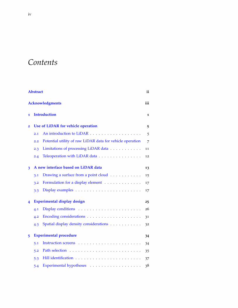
Figure 4.1: One of the sourcehills for the LiDAR scan data,generated for this experiment.

The simulated hills used in this experiment were based on agrid of triangles, each with a nominal vertical slope of 30

◦ in the ydirection, away from the sensor. To modify what would otherwise bea completely smooth slope from bottom to top, the internal verticesof the triangular grid had normally distributed perturbations applied,


to produce the kind of “discretely mogulled” hill shape like the oneshown in Figure 4.1 on the preceding page. The reason to apply thesepertubations only to internal vertices of the grid—that is, excludingthose along the outer perimiter of the hill—was to maintain anidentical global hill profile across all hills.

The simulated LiDAR scanning was performed from a fixed originpoint with rays emanating such that they would intersect the non-deviating base hill at equal spacings2, with an average density of 2 As discussed in Display density

considerations, Section 4.3 on page 32.16 points per square unit on a hill that is 10 units wide and 6 unitsin depth. A schematic of this arrangement and the relative positionof the scanning origin, located 8 units in front of the hill and 2.5units above ground level3, is illustrated in Figure 4.2. The displaced 3 At the hypothetical location of the

virtual LiDAR scanner located on thevirtual vehicle.

viewpoint4 is 7.5 units directly above scanning origin—that is, 10

4 Not shown in the figure, but discussedbelow.

units above the ground.

Figure 4.2: An illustration ofthe hill being scanned froma central point. In this figureonly 1/9

th of the laser scansare shown, for clarity. Thisis not a spherical scan likea typical LiDAR observation,but rather the angle betweenconsecutive beams varies asto evenly sample the hill, asdiscussed later in Section 4.3 ondisplay density considerations.

There were two tasks that subjects were asked to perform foreach presentation. First, while looking at the display based on thesimulated LiDAR point cloud obtained from a hill, the subject wasasked to identify the best path to traverse the hill from one of the threebottom triangles up to one of the three top triangles, where a ‘traversal’required passing through triangles which share a common edge,as illustrated by the blue highlighted triangles in Figure 4.3 on thenext page. The ‘best path’ was defined as the traversal which wouldminimize the slope magnitudes encountered on the traversal. Thiswas evaluated using an algorithm described in detail in Appendix Bon page 67.

After identifying the best path to traverse the hill, the participantwas presented an array of four similar hills, three of which weredistractors, and was asked to identify which hill was most likelythe one which the LiDAR display was based on. This selection wasperformed without the LiDAR display visible at the same time.

4.1 Display conditions

In this experiment, four display styles and two viewpoints for thesedisplay styles were used. To compare my proposed design5 to a 5 See Chapter 3 on page 13 for a

complete description.


Figure 4.3: An exampletraversal for the hill shownin Figure 4.1, with the hillsurface colored by local slopemagnitude, using the colorscale below. The highlightedtraversal, shown with blueoutlines around path triangles,is the best possible path for thisparticular hill.

simple presentation of a LiDAR point cloud, it seemed appropriateto consider the redundantly displayed slope information bothseparately and together—that is, orientation alone, color alone,and orientation combined with color. In addition, to be as fairas possible to the raw LiDAR point cloud condition, rather thanpresenting a monochrome grid, the points were encoded withdifferent colors based on distance measured in the forward direction,a not-uncommon display style for point clouds. Each of the displaystyles was rendered from the sensor point of view, as well as from avantage point 7.5 units higher than the sensor point of view, lookingforward and down (diagonally) at the display elements. Thesedisplay conditions will be referred to as undisplaced and displacedviews respectively, with the respective abbreviations of U and D.

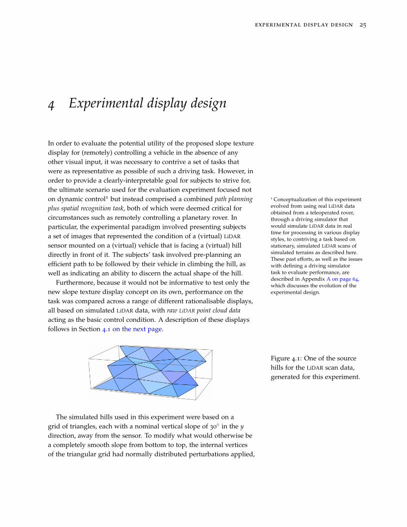
The full list of display conditions can be found in Table 4.1 on thefollowing page, along with abbreviations used throughout the report.

As discussed in Section 2.2 on page 7, an undisplaced view doesnot show any variation in spatial density of the points displayed,whereas a displaced view does. As discussed in the forthcomingExperimental hypotheses (Section 5.4 on page 38), I expected thatsubjects would benefit from this redundant encoding provided by thedisplaced viewpoint for the hill shape recognition task.

Examples of all eight display conditions are shown in Figures 4.5to 4.13 on pages 28–30, for the same hill shown in the beginning


Display style Viewpoint Abbreviation

Points with distance encodedby color

Undisplaced DistanceU

Displaced DistanceD

Squares with slope encoded byorientation

Undisplaced ShapeU

Displaced ShapeD

Squares with slope encoded bycolor

Undisplaced ColorU

Displaced ColorD

Squares with slope encoded byorientation and color

Undisplaced Shape+ColorU

Displaced Shape+ColorD

Table 4.1: Display conditionsand associated abbreviationsused in the experiment.

of this chapter (Figure 4.1 on page 25). Note that a discussionof the method used for color encoding is presented in EncodingConsiderations, Section 4.2 on page 31.

Figure 4.4: The distanceencoding color scheme usedin the Distance display styles.

Figure 4.5: DistanceU:Undisplaced viewpoint, withdistance encoded by color. Notehow the undisplaced view doesnot show any spatial variationof point density due to the hillshape, only a regular patternthat is the result of the laserscan distribution.


Figure 4.6: DistanceD:Displaced viewpoint, withdistance encoded by color. Notehow, in contrast to Figure 4.5,there are spatial point densityvariations due to the hill shape.

Figure 4.7: ShapeU:Undisplaced view squares,with local slope encoded byorientation of the squares.

Figure 4.8: ShapeD: Displacedview squares, with local slopeencoded by orientation of thesquares.

Figure 4.9: The slope encodingcolor scheme used for the Colorand Shape+Color display styles.


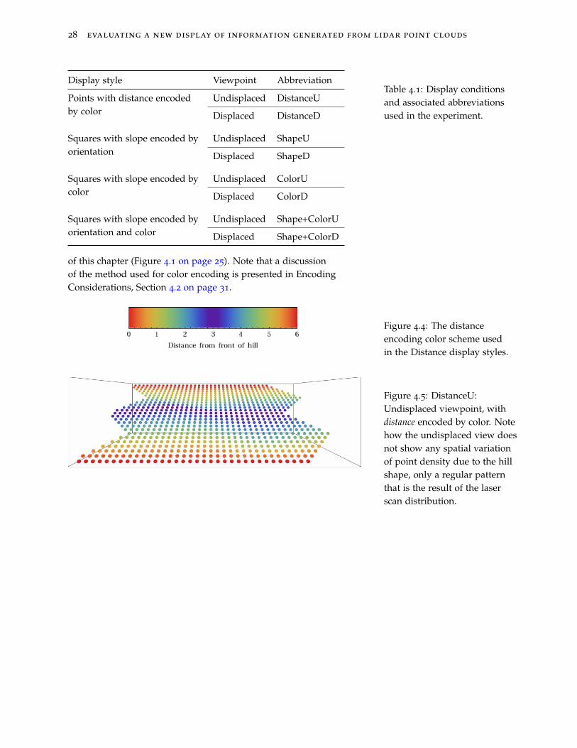
Figure 4.10: ColorU:Undisplaced view points, withlocal slope encoded by color.

Figure 4.11: ColorD: Displacedview points, with local slopeencoded by color.

Figure 4.12: Shape+ColorT:Undisplaced view squares,with local slope encoded byorientation and color of thesquares.

Figure 4.13: Shape+ColorD:Displaced view squares,with local slope encoded byorientation and color of thesquares.


4.2 Encoding considerations

It was my goal to design the display conditions to most fairlycompare the proposed display to a conventional point cloudrendering. Doing so required several design considerations.

Although one of the goals of the proposed texture display wasclarity when viewed from the sensor perspective—ie, close to wherethe driver of a remotely operated vehicle might be located—it wasnecessary that this condition be tested in order to validate the design.This was in spite of the fact that it was assumed an undisplaced viewof a LiDAR point cloud would not be the fairest of comparisons, sincein practice an operator would probably not choose an undisplacedviewpoint while looking at LiDAR data represented as points.Therefore, both a displaced and undisplaced case were tested foreach display style.

It is not uncommon to see LiDAR color-coded point clouds, often ina rainbow gradient. A rainbow scheme is in fact frequently used as adefault encoding scheme, unfortunately often in situations where it isnot appropriate due to the fact that color variations within rainbowschemes are not perceived as varying linearly6. 6 Rogowitz, B. E., & Treinish, L. A.

(1995). Why should engineers andscientists be worried about color? Tech.rep., IBM Thomas J. Watson ResearchCenter

It seemed that there were two ‘fair’ approaches to this problem: tochoose the same genre of color gradient for distance encoding as wellas for slope encoding, while making sure to use different hues so thatsubjects would not confuse the encoded variables (due to the withinsubjects design), or to choose the best possible color scheme for eachdisplay, while attempting to maximize performance in each displaycondition. I decided on the latter approach, to strive to compare best-case display conditions.

While I was experimenting with color scale options, it was clearthat with the gradients provided in Mathematica a good enoughresolution could not be obtained to perceive slope across the entiredistance range. I also tried repeating the available gradients, suchthat the entire color range would be reached for the first half of depthvalues, and then the same range would repeat for the second half.Because of the hard edge this repetition created at the midpoint, Iswitched to a ‘mirroring approach,’ where the second half wouldreverse through the possible gradient values. In the end I decidedto use a rainbow coloration with an inverted repetition to encodedistance, as shown in Figure 4.4 on page 28. Even with the perceptualargument against using a rainbow color scheme, this seemed likethe best way to allow for high-resolution comparisons of distancebetween neighboring points. This scale, of course, is an ambiguousone: red maps to both the nearest and the farthest points, forexample. However, this coloring function is not being recommended


for real-world use. Rather, it was selected because for this task thisparticular ambiguity is not an issue, and this color scheme doublesthe effective local resolution of distance data.

As for the encoding of distance rather than height, in a typicalcase, one would like to be able to discern obstacles without requiringknowledge of the range to those obstacles in advance. For thatreason, it may make some sense to color code LiDAR data by height.In the present case, with a ramp hill at a fixed known distance, eitherheight or distance encoding should produce similar results, thedifference being which feature is more salient between steep andshallow segments. Through height encoding, a steeper region has afaster gradation in color, and a shallow region has a lower gradation.The inverse is true for distance coloration. The selection of a distance-based coloration was based, like the gradient selection, on my ownpreference while comparing displays.

The slope coloration gradient has a different use: unlikecomparing gradients locally in the distance encoding display, wherethe ambiguity due to a repeating gradient was not a problem,here slope values would be compared between regions withdiscontinuities in slope. The chosen scale, therefore, would needto lend itself to absolute comparisons. And as mentioned earlier,the scale that encodes slope should be very different from the scalethat encodes distance, so that subjects do not confuse the two. I usedMathematica’s AvocadoColors for slope encoding, with all slopesunder 5

◦ colored black, and all slopes greater than 33◦ as yellow. This

color scale is shown in Figure 4.9 on page 29.Finally, the proposed display style encodes slope in both a shape

and a color parameter. However, testing this condition alone wouldnot tell us if only one of these variables was responsible for taskperformance, or if it was indeed a combination of the two. Therefore,it made sense also to include a shape-only and color-only encoding ofslope as display conditions for evaluation, as mentioned earlier.

4.3 Spatial display density considerations

With a normal LiDAR sensor, one scans radially with equal angulardensity, resulting in greater point cloud spatial density for nearersurfaces, with a drop-off roughly with the square of distance. In theexperiment, however, I did not want to complicate slope estimationperformance by having the experimental task difficulty vary withposition in the scan results, as there would be a perceptual advantagefor close triangles over far ones. That said, a LiDAR scan has spatialdensity variations due to slope variation7 which would be important 7 as well as distance variation

to recreate. To balance these ideas, I implemented a scanning pattern


that was specifically ‘aimed’ at the base 30◦-slope hill that each

experiment hill was generated from. This is illustrated in Figure 4.14.

Figure 4.14: A cross-sectionof the hill being observed.Note that the average slope hill,shown in red, would receivean even spatial distributionof LiDAR points. Instead theactual hill, shown in blue, has ahigher point density at a steepsegment and a lower density ata shallow segment.If the scan is performed on the base hill, the point sampling

should be an equally-spaced grid8. As we see in the figure, this 8 The analogous surface for aconventional LiDAR scanner wouldbe as if the sensor origin was at themiddle of an ellipsoid shell, where thevertical and horizontal radii would beselected to match the elevation andazimuth angle spacings respectively.

ray dispersion pattern still results in the same sort of point densityvariation due to slope variation, while also providing the sameaverage measurement density across the hill. This should make theslope estimation performance on any given hill segment invariant fordifferent positions on the hill.

The second density consideration is the area that appearscolored in the display. Since most of the display conditions usecolor to encode data, it made sense to keep the same amount ofcolored area constant in the display across display conditions. Tosolve this design problem, displays were first computed from anundisplaced perspective for many hills in both the points and squaresconfigurations, with black display elements. An image histogramwas computed over each series of displays, and point size was varieduntil the histograms matched, in terms of proportion of black versuswhite in the image, for all of the square and point sizes.

During this operation, a discontinuity in the rate of change ofthe black to white ratio was observed in the histograms of varyingpoint size. This was the result of point diameter reaching a valuewhere points started to overlap near the top of the display. It was notactually possible to match histograms because of this overlappingpoint region in the point diameter space, unless square size wasreduced dramatically. Instead, the point display was modified to use3D spheres instead of 2D points, which would therefore have a slightprojected size decrease for more distant points.


5 Experimental procedure

Nine male subjects were recruited to participate in this experiment,following a within-subjects random block design with eight displayconditions1. The experiment was restricted to males with no defects 1 Four display styles and two

displacement lengths, explained inDisplay conditions, Section 4.1 onpage 26

in color vision, and wearing any corrective lenses they wouldrequire, in order to avoid both gender variation in spatial perceptionas well as the effects of misinterpreting the displays due to colormisinterpretation. Only data from eight subjects was later analyzed,as the results from one subject was rejected as he appeared notto take the experiment seriously. The details of this exclusion areoutlined in Appendix D on page 83.

Eight hills were generated and were used as the source for theLiDAR point clouds for all subjects. Each participant performed boththe path selection task as well as the hill identification task for thesame eight hills, in a randomized order for each of the eight displaycondition blocks, for a total of 64 presentations per participant.

A ninth hill was generated for the example display in theinstruction screens, as well as a single-presentation training blockat the beginning of each experiment. This training block was toallow the participants a chance to learn to use the interface forentering their selections. The display condition used for this singlepresentation was selected at random for each participant, so as to notsystematically bias the experiment with more experience providedfor any single display condition. The randomized blocks of displayconditions aimed to minimize inter-presentation bias, as well aseliminate the factors of learning and improving in performance2 in 2 Or alternatively, becoming fatigued

and bored with a decrease inperformance. However, as theexperimenter, I would like to thinkthat my subject enjoyed choosing a pathfor the 50

th time just as much they didfor the first time: quite a lot.

both tasks through the duration of the experiment.

5.1 Instruction screens

The experiment software interface presented the eight displaycondition blocks in a randomized order, with a set of initialinstruction screens at the very beginning of the experiment. Foreach block, an instruction screen explaining that specific conditionwas shown, and then the 8 hills were presented in randomized order.

experimental procedure 35

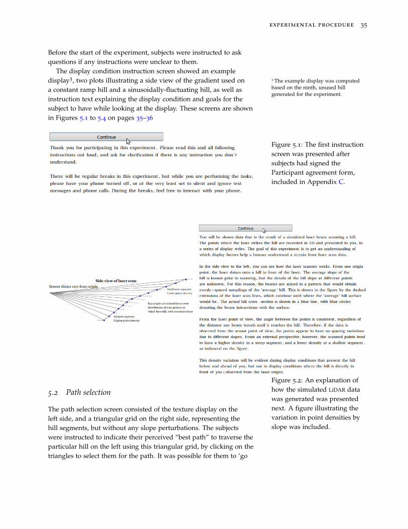
Before the start of the experiment, subjects were instructed to askquestions if any instructions were unclear to them.

The display condition instruction screen showed an exampledisplay3, two plots illustrating a side view of the gradient used on 3 The example display was computed

based on the ninth, unused hillgenerated for the experiment.

a constant ramp hill and a sinusoidally-fluctuating hill, as well asinstruction text explaining the display condition and goals for thesubject to have while looking at the display. These screens are shownin Figures 5.1 to 5.4 on pages 35–36

Figure 5.1: The first instructionscreen was presented aftersubjects had signed theParticipant agreement form,included in Appendix C.

Figure 5.2: An explanation ofhow the simulated LiDAR datawas generated was presentednext. A figure illustrating thevariation in point densities byslope was included.

5.2 Path selection

The path selection screen consisted of the texture display on theleft side, and a triangular grid on the right side, representing thehill segments, but without any slope perturbations. The subjectswere instructed to indicate their perceived “best path” to traverse theparticular hill on the left using this triangular grid, by clicking on thetriangles to select them for the path. It was possible for them to ‘go


Figure 5.3: The path selectionand the hill identification taskswere explained in the thirdinstruction screen.

Figure 5.4: The type ofinstruction screen that precededeach display condition block,showing an example of thedisplay condition, a scale in theform of both a constant-sloperamp hill and a ‘moguled’hill, as well as instructiontext describing the displaycondition.

experimental procedure 37

back’ and deselect triangles if they decided to change the selectedtraversal.

The interface did not allow for the entry of redundant paths—if apath contained a possible shortcut, the subject would not be able toselect that path4. 4 Fortunately, trying to do this was

extremely uncommon: only one subjectattempted to enter a redundant path,and asked why he could not selecta triangle. After the redundancywas pointed out, he understood anddeselected a portion of the path.

After a path was completed, a “Save and continue” buttonappeared on the screen. At this time, the subject would look atthe display to remember the hill shape for the subsequent hillidentification task, outlined below.

Figure 5.5: The display shownfor a path selection task,with the perceived best pathindicated. When the lasttriangle was selected, the “Saveand continue” button appeared.

5.3 Hill identification

After selecting “Save and continue” on the path selection screen, ahill identification screen would be shown, comprising three distractorhills and the correct response hill, shown simultaneously individuallyrotating (as per Figure 5.7 on the following page) within a 2× 2 grid,as shown in Figure 5.6.

Figure 5.6: The hill identi-fication screen presented toa subject, with the selectionbuttons arranged to the leftand right of the grid of rotatinghills.

Subjects were instructed to select their choice of hill that theybelieved corresponded in shape to the one they had just traversed,by clicking one of the four buttons corresponding to the four hills inthe grid. When one of the buttons was clicked, a “Save and continue”


Figure 5.7: A rotating view ofa hill. Click to view animation.Each of the four hill optionswere animated continuously asshown when presented duringthe hill identification screen inFigure 5.6, in order to resolvethe ambiguities of showing astationary image of the hill.

button would appear on the screen to confirm the selection. Beforeconfirming, the subjects could still select a different hill by clickingon a different button, which would deselect the previous button ifthey so desired.

5.4 Experimental hypotheses

It was hypothesized that a displaced view would improve resultsfor both path selection and hill identification tasks. Viewpointdisplacement provides a spatial density variation in the displayoutput, which reflects hill geometry, and should therefore assist inthe understanding of a hill for all display styles. That said, I expectedviewpoint displacement to be a larger factor for the base case displaystyle for which distance is encoded by color, as that display providesthe least obvious sense of hill geometry. I also expected viewpointdisplacement to be a smaller factor when the display elements weresquares rather than points, because they convey a sense of hill shapethat is still present in the undisplaced view.

The encoding of slope by square orientation was expected tobe beneficial to the hill identification task. Since the orientation ofsquares on a surface encodes slope direction as well as the magnitude,I expected that a better sense of the hill shape would be conveyed,beyond encoding either slope magnitude or just distance at anyposition.

results 39

6 Results

Separate analyses were carried out for both the (local) path selectionperformance and the (global) hill identification performance.

For simple referral to the display conditions, the abbreviationsintroduced in Table 4.1 on page 28 will be used throughout thischapter.

6.1 Path selection performance

A path selection score was devised to evaluate how well anyselected path met the task requirements of minimizing the slopesencountered. A lower score represents a better selected path, witha score of zero applied to the best possible path for the hill. Asimple explanation of the scoring function is that it increases as theencountered segment slopes of a traversal increase, in a way thatapplies a greater penalty to the steepest segments.1 All scores less 1 For a detailed explanation of how the

scoring function works, see Appendix Bon page 67.

than one indicate nearly equally good path selections, scores greaterthan five indicate a poor path selection, and scores greater than 10

indicate a very poor path selection.Figure 6.1 on the following page shows the combined performance

across participants, by display condition. We see that DistanceUdisplay condition has the largest spread in path scores, as well asthe greatest median score. The displaced viewpoint variant of thisdisplay condition, DistanceD, seems to perform better, but not as wellas the slope encoding display conditions.

We can furthermore see that the scores for the Shape, Color andSlope+Color display styles follow a truncated distribution, with ahigh frequency of zero and near-zero scores.

To examine performance in more detail, it is useful to look atpairwise comparisons between display conditions. Figure 6.2 onthe next page shows the performance for individual participants,looking at particular hills under both the DistanceU and DistanceDconditions. The distribution of scores seen in Figure 6.1 on thefollowing page are evident in this plot, as the points in the xdirection represent the DistanceU path selection scores, and the


Figure 6.1: Summarizedpath selection performance.Each point represents thescore for a path selected fora particular hill and displaycondition. (Recall that betterscores correspond to smallernumbers.) Interquartile rangesare indicated in light blue foreach display condition.

points in the y direction are the DistanceD path selection scores. Anypoint lying on the positive diagonal therefore represents a case forwhich the same subject obtained the same score under both displayconditions for that particular hill.

Figure 6.2: A pairwisecomparison in path selectionscores for DistanceU comparedto DistanceD, to examine theeffect of a displaced viewpointin the Distance display style.

This plot thus allows us to see whether individual subjects hadequally good performance or equally poor performance in bothconditions, versus whether there is a tendency for one of the twodisplay conditions to improve the path selection performance for the

results 41

same hill and the same subject. The cluster of points evident alongthe x axis (which represent very low scores in the vertical DistanceDcondition (the y axis) and a range from passable to bad scores inthe DistanceU display condition) seems to suggest that viewpointdisplacement improved performance in the distance-encoding displaycondition, as anticipated.

Pairwise comparisons such as the one discussed above can bemade also between every set of display conditions. A multiplot of allpairwise comparisons in path selection performance is presented inFigure 6.3 on the next page.

This comparison allows for qualitative comparisons of differentperformance between conditions, including an examination of theeffect. of viewpoint displacement. For the D compared to U plots,it appears as though only for the previously-discussed Distancecomparison have a center of mass of the points to one side of thediagonal (in the lower right compared to the upper left, suggestingthat DistanceD is better than DistanceU).

Analyzing the path performance data quantitatively now, thescore measures come from a truncated distribution, so a parametricanalysis is not valid. Since a large number of scores are exactly orvery close to zero, it was concluded that no set of transformationswould map these results to a normal distribution and thereforethat a non-parametric analysis must be used. Path selection scoreswere floored to consider all scores less than 1 to be equally goodperformance, so for a rank-based analysis all scores less than 1 willbe considered a tie.

The results were analyzed using Friedman’s ANOVA, a non-parametric repeated measures analysis of variance by ranks. Theanalysis, the results of which are summarized in Table 6.1 on page 43,showed that display condition had a significant effect on pathselection performance, χ2(7) = 187, p < 0.05.

Since Friedman’s ANOVA showed significant differences,individual pairwise comparisons were performed using Wilcoxon’ssigned rank test, in order to examine the effect of display style,as well as the effect of viewpoint displacement on path selectionperformance.

Each display style was compared to DistanceU, where the scores(median score = 3.40) had significantly worse ranks than each ofthe undisplaced scores for other display styles, as summarized inTable 6.2 on page 44, each with p < .05:

As for viewpoint displacement, an additional Wilcoxon’ssigned rank test was carried out and, consistent with the earlierqualitative analysis, showed that only ColorD (median score = 2.49)had significantly better ranks than undisplaced variant ColorU


Figure 6.3: Path selectionperformance, in pairwisecomparisons between displaytypes. Plots are in the samestyle as Figure 6.2

results 43

Homogeneous SubsetsSubset

1 2 3

Display condition1

Shape+ColorD 3.375

Shape+ColorU 3.594

ColorU 3.648

ColorD 3.656 3.656

ShapeD 4.539 4.539

ShapeU 4.664

DistanceD 5.656

DistanceU 6.867

Test Statistic 8.384 6.805 5.641

Sig. (2-sided test) .078 .033 .018

Adjusted Sig. (2-sided test) .123 .086 .068

Homogeneous subsets are based on asymptotic significances. Thesignificance level is .05.1Each cell shows the sample average rank.

Table 6.1: The mean ranks ofpath selection performance bydisplay condition. Note thata lower rank means a lowerscore, which is better in thiscase. The three homogeneoussubsets of ranks were found tobe significant by performingmultiple grouped comparisonsof display conditions, whichare shown in the three verticalstripes of highlighted ranks.The non-overlapping set of theDistance ranks suggest theydo not come from the samedistribution as the other sixdisplay styles that encode slope,p < .05.

(median score = 3.50), z = −3.51, p < .05, r = −.44. This wasthe observation made at the beginning of this section by examiningthe effect of displacement using the path selection performancemultiplot.

6.2 Hill identification performance

Recall that the hill identification task2 had subjects identify a target 2 Described in the Hill identification,Section 5.3 on page 37hill that was presented alongside three distractors. In selecting the

target hill, chance performance therefore equals a 25% probability ofbeing correct, or equivalently, a 75% probability of being incorrect.Figure 6.4 on page 46 shows the cumulative hill identificationperformance across all participants.

In the figure, we see that the hill identification task showedcorrect response rates better than chance odds (indicated by a redline at 25display styles (Shape, Color, Shape+Color) than Distance.Interestingly, displaced scores were only slightly higher for alldisplay cases except for Shape, where there were many more correctresponses given the ShapeU display than ShapeT.

A second representation of overall performance in the hill selectiontask is given in Figure 6.5 on page 47, which is similar to Figure 6.4in that it again represents proportion of correct responses for the 8

different display conditions. This figure goes beyond the previousone, however, by taking into account three other factors:


Ranks

N Mean Sum ofrank ranks

ShapeU - DistanceU

NegativeRanks

45a

26.42 1189.00

PositiveRanks

6b

22.83 137.00

Ties 13c

Total 64

ColorU - DistanceU

NegativeRanks

53d

29.35 1555.50

PositiveRanks

3e

13.50 40.50

Ties 8f

Total 64

Shape+ColorU -DistanceU

NegativeRanks

54g

27.50 1485.00

PositiveRanks

0h .00 .00

Ties 10i

Total 64

Test Statisticsj

ShapeU ColorU Shape+ColorU- DistanceU - DistanceU - DistanceU

Z -4.940k -6.197

k -6.409k

Asymp. Sig. (2-tailed) .000 .000 .000

Table 6.2: The results of aWilcoxon’s signed rank testbetween DistanceU and eachof the listed display conditions,each of which had a significantrank improvement, p < .05

a. ShapeU < DistanceUb. ShapeU > DistanceUc. ShapeU = DistanceUd. ColorU < DistanceUe. ColorU > DistanceUf. ColorU = DistanceUg. Shape+ColorU < DistanceUh. Shape+ColorU > DistanceUi. Shape+ColorU = DistanceU

j. Wilcoxon Signed Ranks Testk. Based on positive ranks.l. Based on negative ranks.

results 45

Ranks

N Mean Sum ofrank ranks

DistanceD -DistanceU

NegativeRanks

35a

29.60 1036.00

PositiveRanks

16b

18.13 290.00

Ties 13c

Total 64

ShapeD - ShapeU

NegativeRanks

15d

14.07 211.00

PositiveRanks

14e

16.00 224.00

Ties 35f

Total 64

ColorD - ColorU

NegativeRanks

6g

5.42 32.50

PositiveRanks

5h

6.70 33.50

Ties 53i

Total 64

Shape+ColorD -Shape+ColorU

NegativeRanks

8j

5.81 46.50

PositiveRanks

3k

6.50 19.50

Ties 53l

Total 64

Test statisticsm

DistanceD ShapeD ColorD Shape+ColorD- DistanceU - ShapeU - ColorU Shape+ColorU

Z -3.510n -.144

o -.045o -1.218

n

Asymp. Sig. (2-tailed) .000 .886 .964 .223

Table 6.3: Wilcoxon’s signedrank test results to determinethe effect of viewpointdisplacement.

a. DistanceD < DistanceUb. DistanceD > DistanceUc. DistanceD = DistanceUd. ShapeD < ShapeUe. ShapeD > ShapeUf. ShapeD = ShapeUg. ColorD < ColorUh. ColorD > ColorUi. ColorD = ColorUj. Shape+ColorD <Shape+ColorUk. Shape+ColorD >Shape+ColorUl. Shape+ColorD =Shape+ColorU

m. Wilcoxon Signed Ranks Testn. Based on positive ranks.o. Based on negative ranks.


Figure 6.4: Correct responserate, shown by light greenbars, for the hill identificationtask, by display condition.The complementary incorrectresponse rate is shown stackedin red. The horizontal redline indicates the boundaryat which chance performanceoccurs.

• differences in performance by individual subjects

• the time taken by subjects to make their responses

• the performance on individual hills

In this plot, we observe large inter-participant differences. Inparticular, subject 2 had a large proportion of incorrect responsesdistributed across display conditions.

Comparing an undisplaced viewpoint with a displaced viewpointwithin a subject and display style is a matter of comparing the leftand right sides of a pair of columns, which are separated with thinwhite lines. When doing so, we see that subjects 7 and 8

3, tended 3 the two best-performing participantsin the hill identification task in terms ofcorrect response rate

to perform similarly or better for the displaced viewpoint variantsof all the display styles. However, there are also situations plottedwhere displaced performance was worse for a participant in aparticular display style. For example subject 5 performed better inhill identification for both DistanceU over DistanceD and ShapeUover ShapeD.

All horizontal stripes across the display represent the effect ofa particular hill. It appeared to me that the 6

th hill, counting fromthe top, had an unusually large number of red squares. To examinethis further, the confusion matrix in Table 6.4 on the next page wastallied for the data from all eight participants, in the eight displayconditions:

From examining the confusion matrix, we see that there areindeed more misses for the 6

th hill than for others. It’s interestingto note that the most frequent error mode was a confusion where

results 47

Figure 6.5: Time to successfulcompletion for the hillidentification task, groupedby subject. (Subject numbersare shown in parentheses.)Each row of data represents aparticular hill, with the sameordering across subjects, andeach column is a displaycondition. Thin white linesseparate display styles, tosimplify the comparisonbetween displaced andundisplaced viewpointperformance. Task completiontimes are encoded accordingto the density scale shownat the bottom, where darkerrepresents faster and lighterrepresents slower performance.White squares indicate that theresponse time was greater than40 seconds Finally, dark redsquares indicate an incorrectresponse.

ResponseTarget 1 2 3 4 5 6 7 8

1 43 6 2 2 4 2 3 2

2 4 33 2 3 7 8 5 2

3 6 3 38 2 6 4 3 2

4 3 0 2 44 2 3 6 4

5 0 1 1 9 40 2 7 4

6 5 0 1 15 7 26 6 4

7 1 2 5 5 0 4 44 3

8 2 2 2 2 5 1 5 45

Table 6.4: Confusion matrixbetween target hills in therows, and a tally of responsehills by column. Perfectperformance would consistof 64 correct responses (thetotal number of presentationsper hill in the tally, 8 hills× 8 participants) along thediagonal of the matrix, with 0

incorrect responses in all otheroff-diagonal positions.


a display based hill 6 was presented, and hill 4 was the response(15 occurrences), but we do not see the same high confusion ratewhen hill 4 was presented with hill 6 as the response (3 occurrences).Looking at the two hills, compared in Figure 6.6, it appears thatneither has a particularly large variation in slopes, and both areflatter on the left side than the right side.

Figure 6.6: A comparisonbetween the most frequentlyconfused hills in theexperiment. The top hill (4)is thought to be the bottomhill (6) in 15 presentations,whereas the bottom hill is onlyconfused for the top hill in 3

presentations.

A Kolmogorov-Smirnov test of normality was performed on thecorrect response rate data, and only the ShapeU was found to besignificantly non-normal, D(8) = 0.37, p < .05.

Select pairwise comparisons were made with a paired-samplesT-test, which showed no significant (p < .05) difference for viewpointdisplacement vs non-viewpoint displacement of any evaluated case.

Comparisons were also made between display conditions in thedisplaced case, and the differences that were found to be significant(with d f = 7) are presented in the following table. The resultsindicate a very substantial performance improvement for the slopetexture display, especially as a consequence of the slope encoding bymeans of color:

Conditions compared Lowerlimit

Mean Upperlimit

ShapeD - DistanceD 2.1% 17% 36%ColorD - DistanceD 6.6% 33% 59%Shape+ColorD - DistanceD 12% 33% 54%

Table 6.5: Differences in meancorrect response rate for eachof the three slope-encodingdisplaced viewpoint displayconditions (ShapeD, ColorD,and Shape+ColorD) relativeto the displaced viewpointdistance-encoding condition(DistanceD). In addition tomean differences, the lower andupper 95% confidence limitsare given, as analyzed withpaired-samples T-tests.

Finally, as a continuation of the preceding observation, paired-samples T-test comparisons were carried out to determine if themethod of encoding slope, via color vs via orientation of the display

results 49

element, affected hill identification rates. The analysis produced onlyone significant differences pair, again with d f = 7, as shown in thefollowing table. The finding again supports the importance of colorfor communicating local slope information in support of hill shaperecognition.

Conditions compared Lowerlimit

Mean Upperlimit

Shape+ColorD - ShapeD 4.8% 16% 26%

Table 6.6: Difference inmean correct responses (inpercentage) for Shape+Colorcondition relative to Shape,both with displaced views.In addition to the meandifference, lower and upper95% confidence limits are given,as analyzed using paired-samples T-tests.


7 Discussion

It was not surprising that encoding slope with color—whetherwith or without redundantly also encoding it in shape—improvedpath selection performance, which was a task chosen to measureslope estimation ability. The task revolved around making slopecomparisons at various points along each hill, and with slopeencoded by color, this was just a matter of comparing colors withineach presentation1. Estimating the slope of any point given a color- 1 To me, this triviality was the weakest

part of the experimental design.Unfortunately, the task of designingtasks to accurately measure displayunderstanding is not nearly astrivial. Ideally, the performance in ateleoperation task would be used asa measure for display utility, but thatrequires a very clear definition of taskgoal. See the discussion in Appendix Aon page 64 for more on is topic.

coding by distance was more challenging, and not surprisingly,subjects performed worse.

Slope estimation performance for distance encoding wasfurther improved by providing a ‘displacement’ between the datapresentation viewpoint and the sensor perspective in the case ofcolor encoding distance—ie, DistanceD relative to DistanceU. Thedifference between a displaced and undisplaced view manifestsitself here through the encoding of shape information via spatialdensity variation. Viewpoint displacement did not significantlyimprove slope estimation performance (ie, path selection) for anyother display style.

More interestingly, viewpoint displacement also did notsignificantly improve performance for hill identification for anydisplay style, even distance encoding.

I had expected an improved performance in hill identificationdue to viewpoint displacement because the spatial density variationconveys structure in a systematic way. However, recalling the hillidentification performance presented in Section 6.2 on page 43,there were substantial inter-subject variations in performanceon this task. Furthermore, recall that subjects 7 and 8 performedsimilarly or better in the displaced conditions, most notably in thedistance encoded display. There were also situations where displacedperformance was worse for a participant in a particular display style.Although these observations of individual results do not containsufficient data to support a statistical inference, comments from someparticipants shed light on the observed phenomenon.

Both subjects 7 and 8 independently noted that they were actively

discussion 51

going against their intuition while interpreting the density variationsin the display, particularly during the ShapeD block. Subjects 5

and 6 noted furthermore that they found it difficult to ignore theiropposing intuition in interpreting density variations. It had beennoted, by inspection of Figure 6.4 on page 46 in the previous sectionthat ShapeU had surprisingly outperformed ShapeD in the hillidentification task. Why might this be the case? Example Shapedisplays are presented in Figures 7.1 and 7.2.

Figure 7.1: A displacedviewpoint rendering of theShape display condition(ShapeD), where the lowdensity regions at the bottomright and near the top leftboth mean that the slopethere is low, indicating shallowentrances to a concave region.Some subjects mentioned thatthey would tend to interpretthese instead as steep portionsof a convex region.

Figure 7.2: An undisplacedviewpoint rendering ofsquares with slope encodedby orientation (ShapeU).

I did not consider this in my hypothesis, but I postulate that,although ShapeU does not provide a density variation representativeof hill shape the way that ShapeD does, there is nevertheless anadvantage to the ShapeU display. Note that from the elevatedperspective in ShapeD, all parts of the hill become closer toperpendicular to the viewer. This, in turn, reduces the foreshorteningof shallow segments, and reduces the spread of projected textureelements. The foreshortening of squares in a texture display hasbeen shown to be an effective means to convey slope information2, 2 Todd, J.T. & Akerstrom, R.A. (1987).

Perception of three-dimensional formfrom patterns of optical texture. Journalof Experimental Psychology: Humanperception and performance, 13. 242–255.

and in this case, this form of slope encoding is being reduced inmagnitude. This is the result of the specific geometries used in thedisplaced perspective, where the view vector has a smaller anglewith the average surface normal than the undisplaced perspective


view vector’s angle with the average surface normal. It is thereforehypothesized that reducing the angle between the view vector andthe average surface normal in turn reduces the effect of texture elementforeshortening (for tangentially-oriented texture elements), resulting in adecreased efficacy in conveying surface geometry.

So why does Shape+ColorD still outperform Shape+ColorU? Itshould be noted that from the statistical analysis, the performance inthe two conditions come from different distributions. It could be thatthere is no performance difference. That said, the best performingsubjects did have a tendency to perform better in hill identificationwith the Shape+ColorD display condition than the Shape+ColorUcondition. This could be attributed to the fact that slope magnitudeis already encoded in the display element color, and the orientationprovides a better sense of the hill geometry, improving identificationperformance. Contrast this with the ShapeD display, where theslope magnitude information is presented from the spatial densityvariation of the display elements (as discussed earlier, this wassometimes in conflict with what subjects would intuitively assume),and the now-diminished element foreshortening effect.

Although viewpoint displacement did not have a statisticallysignificant effect on hill identification performance, the displaystyle did have a statistically significant effect. Each of the Shape,Color, and Shape+Color variants of slope encoding resulted inimproved rates of correct hill identification compared to displayingdistance encoded by color3. For the global task of hill identification, I 3 The comparison used here is for the

displaced condition, for fairness withrespect to the Distance display, eventhough DistanceD was not found to besignificantly different from DistanceU.

interpret this result as showing that there was a demonstrably betterunderstanding of the underlying hill from the data through thesedisplay styles.

Furthermore, in comparison between displaced views of the slopeencoding display conditions, it was shown that hill identificationrates are between 5 and 26% greater when shape and color are usedto encode the slope data compared to just the use of shape.

In summary, although there is not a statistically grounded reasonto say which of the slope-encoding display styles is better whencomparing Shape+Color encoding with Color encoding, it wasclear that all three slope-encoding display styles provided a betterunderstanding of local slope (through the path selection task) aswell as the global shape of the hill (through the hill identificationtask) when compared to the Distance display style. Redundancy inencoding the slope information with both shape and color thereforeseems like it would be the most sensible display style to choose inpractice out of those tested. While a displaced view was useful forthe baseline distance encoding case, the proposed display style wasnot shown to significantly benefit from viewpoint displacement.

discussion 53

Of course, it is entirely possible that the hypothesis of displayeffectiveness benefiting from viewpoint displacement is true, butthe experiment conducted did not have the statistical power to showit. In light of the improved performance of some individual subjectsunder the displaced viewpoint condition, further investigation of thisfactor is recommended.


8 Limitations

As mentioned earlier in a side note at the beginning of the Discussion(Chapter 7 on page 50) I think that the biggest inadequacy in thisexperiment was the much lower difficulty of the path selection taskfor display conditions where slope was encoded by color. I don’tthink a real understanding of the hill geometry was required toaccomplish this task under these conditions; a subject just neededto visually segment the colors into iso-color triangles, and pick apath based on gradient values. That said, there are neverthelesstwo arguments in favor of this measure. First, a ceiling effect wasnot observed in participant performance data, so perhaps the taskwas not as easy as I suspected. Second, the goal was to evaluateperformance related to understanding of slope, and the path selectiontask provided an absolutely definable goal that would not beinfluenced by any tradeoffs made by the subject1. 1 Such as a tradeoff would have been

made if the subjects had been asked topick a shortest non-steep path: whichgoal is more important, path lengthor path slope? What is the differencebetween steep and non-steep?

By running four display conditions in which slope was encoded bycolor (displaced and undisplaced cases, for points as well as squares),but only two conditions where distance was encoded by color(displaced and undisplaced), the subject had twice the experiencewith the color gradient than with the distance gradient. How doesan experimenter balance this? It occurred to me to add two moredistance encoded by color block conditions, with a different set ofhills that would not be used in the statistical analysis. However,with eight display conditions and two tasks for each presentation, Idecided it would be better to accept this bias in experimental designand show the subjects more presentations rather than more displayconditions.

The experiment conducted had only nine subjects, and of thoseonly eight subjects whose data was analyzed. A larger populationsize, or perhaps a longer experiment, would have provided moredata and may have made possible a statistical differentiation betweendifferent slope encoding features (Shape, Color, or both).

The experimental paradigm was based around the use of astationary view of stationary data. In any real application ofLiDAR for operating a vehicle, the sensor egomotion will likely

limitations 55

affect the appearance of the display, as well as the perception ofmotion. Possible future work to investigate this effect is discussedin Section 10.3 on page 59, but generally the use of static LiDAR datais a limitation of my approach.

The subjects were asked if they have deficient color vision at thestart of the experiment, rather than tested for color vision deficiencies.Such a test apparatus was not available to me, and I also wantedto maximize the number of presentations shown to eight displayconditions in two hours. Consequently, the question of colordeficiency was relegated to a survey question that it was assumedsubjects would answer honestly. In reality, some subjects who arecolor blind might be unaware their deficiency, so even an honestanswer may not be the truthful one. It’s entirely possible that asubject struggled with my experiment due to an unbeknownst visualsensory deficiency.

The experimental design was randomized as the subject ran theexperiment. That is to say, for each subject, a random order wasselected for the display conditions. (The same was done for theselection of the single display condition for the training session.)For such a small sample size of eight participants, this should nothave been randomized. Instead, it would have been more appropriatefor the orders to be assigned to subjects in a way that ensured thatthere would not be a systematic bias in display conditions.

Finally, from the point of view of representativeness, thisexperiment used a simulated LiDAR sensor that intentionally samplesthe environment differently than a real LiDAR sensor2. The task was 2 See Section 4.3 for an explanation.

contrived and may not be of sufficient fidelity to make conclusionsabout how an operator would operate a vehicle using real LiDAR

data.


9 Contributions and conclusions

The objective of this thesis was to develop and evaluate a techniquefor presenting LiDAR data to a vehicle operator for conveying anunderstanding of the environment, in a manner that would be moreeffective than a simple rendering of a raw point cloud. Strivingto meet this objective resulted in a series of developments whichcontribute to the research on (remote) driving interfaces based onthree-dimensional non-visual data.

A display technique was proposed wherein a LiDAR point cloud issegmented into (potentially sparse) groups of points, which are theneach approximated by a square that is presented at the geometricmean of those points, tangent to the plane of best fit, and oriented inthe direction of maximum slope. These squares have the ability to becolor-coded based on the value of the slope, with the intention beingthat observers would be able to perceive both local and global slopeinformation on the basis of patterns formed by the individual slopeelements.

An experimental paradigm was developed to evaluate thenew display concept, based on the use of a stationary source ofdata, a second method for computing LiDAR scans was written inMathematica, along with a technique to generate triangular gridhills to be sampled by this new LiDAR simulator. The hills weregenerated with random variation in local geometry, but consistentglobal geometry of the average slope and hill outline. A set ofthese generated hills their simulated LiDAR scans was used in anexperiment in which subjects examined different displays based onthese scans—for perspective shape of surface elements only, coloronly, and shape plus color. All display conditions were contrastedwith a baseline simulation of raw LiDAR point clouds—which wereprogrammed to use color to communicate distance from the sensorsource. The subjects selected a steepness-averse path to traverse eachsimulated hill, and also identified the presented hill from a set ofdistractor hills. A program for administering this experiment (andadaptable for other, similar experiments in the future) was written inMathematica.

contributions and conclusions 57

The experiment showed that the proposed shape texture displayimproved comprehension of the geometries that were sampled inthe point clouds, in terms of both path traversal and hill recognitionperformance.


10 Future work

The ergonomics of operating a vehicle with a LiDAR-based displayhave not been examined in much detail, at least in part because itdoes not seem to be an intuitively obvious sensory mode to usefor aiding a human operator in remote or driver-present controlsituations1, despite the fact that there are situations in which the 1 The example I did find of using a

LiDAR-based display for teleoperationof a rover did include an evaluationof performance, but it was focused onthe effect of the predictive componentof their display. Kelly, A., Chan, N.,Herman, H., Huber, D., Meyers,R., Rander, P., Warner, R., Ziglar,J., & Capstick, E. (2011). Real-timephotorealistic virtualized realityinterface for remote mobile robotcontrol. International Journal of RoboticsResearch, 30(3), 211–226.

data that a LiDAR sensor provides could be of utility. In the limitedscope of this thesis, I evaluated only a small subset of possibledisplay techniques that could potentially improve the model of theenvironment conveyed to the operator. Even within this subset, myevaluation looked at only stationary data presentation—in otherwords, I did not address the potential power of motion parallax forconveying 3D environment information from LiDAR scan data, eitherraw or processed with some kind of derivative slope texture display2.

2 See below for a further discussion ofthis issue

Ofthe numerous avenues for future work, I will discuss some of themore interesting ones that crossed my mind during my time workingon this project.

10.1 Overlapping texture elements

As discussed in the introduction to the proposed interface inChapter 3 on page 13, the texture display proposed in this thesisis very similar to the idea of drawing surfaces using surfels. Theprimary difference is that surfels are intended to overlap withsurrounding surfels to form a continuous rendered surface, intendedto look much like a mesh. In order to evaluate the effectiveness ofshape, the non-overlapping-element texture display was evaluated.However, shape encoding was not found to significantly improvetask performance, and the effects of display density variation wereeven deemed troublesome by some participants3. If the display had 3 See the Discussion, Chapter 7 on

page 50, for more details.intentionally-overlapping surface elements, perhaps performancewould improve even further in displaced performance? This remainsto be seen.

future work 59

10.2 Different coloring approaches

Although the experiment did test the encoding of slope data withcolor, there are other surface properties that could be displayed usingthis modality. Perhaps they would be more useful.

One possibility is to use color for the display of curvature, thederivative of slope data. While this involves another computationalstep, it could conceivably be more practical for some vehicleoperating situations. In other words, perhaps high levels ofcurvature are more of a hazard for becoming stuck4 than the risk of 4 Think of a low car chassis scraping

on a speed bump, or the same vehicle’sbumper scraping starting to go up asudden hill.

slipping/rolling at a steep slope, as has been presumed here throughmy investigation of displaying slope information.

Alternatively, a continuous surface displayed with surfels, asmentioned earlier, could be ‘artificially illuminated’ using theGPU. A virtual light source would be placed in the environment,conveying curvature with a shading that is common in a naturalsetting, which would naturally present a sense of the local geometryto the operator5. A natural illumination approach is also possible 5 Gibson, J.J. (1979). The ecological

approach to visual perception. Boston:Houghton Mifflin.

with a non-overlapping-element texture display such as the oneproposed here, but surface self-shading should be avoided in thatcase.

10.3 The effect of sensor egomotion

The global path planning task and hill identification tasks wereboth using stationary viewpoints observing stationary data. WhileI believe that the proposed display would be useful for operatinga vehicle, I don’t believe that it’s reasonable to infer that a displaywhich conveys environment geometry while stationary willnecessarily do so effectively for time-varying data.

In successive points of normal egomotion, whether in a vehicle,on foot, or via an interface for teleoperation, optic flow is a majorcontributor to the perception of that motion. Different features inan environment appear to have different velocities as we move, andthis flow of texture is understood by the brain at a low level6. In 6 Gibson, J. J. (1979). The ecological

approach to visual perceptionsuccessive point clouds during egomotion, the points do not moveto a nearer location, but rather change content to reflect the newdistances at their measured angles. The operator needs to still usethis display to understand the motion of the vehicle, in conflict withGibson’s observation that optic flow conveys egomotion rather than aset of computations.

This raises two major questions, which warrant, and arguably evenrequire, further investigation. The first question is, while observinga display of LiDAR data generated by a sensor moving through an


environment, would perception of egomotion be negatively affected?The second question is, how might the display design be improvedto better convey egomotion? In addition, it’s possible that sensoregomotion could make display ambiguities unimportant, due to avariation of a structure from motion effect.

During execution of a real task, perhaps the displaced viewpointcould be adjusted by the operator. If a display style is ambiguousin some views, is it still faster to use than an unambiguous displaywhen displacement manipulation time is accounted for? Therewould challenges in task design for an experiment in which thesedisplays are used for a teleoperation task, but such a study would beinvaluable.

My work has only scratched the surface of the challenge ofevaluating new concepts for displaying information using LiDARpoint cloud data. There are further comparisons to be madeabout approaches to displaying the data, as well as evaluating theperformance of these displays, including for non-stationary data.

bibliography 61

11 Bibliography

Boots, B., Nundy, S., & Purves, D. (2007). Evolution of visuallyguided behavior in artificial agents. Network: Computation in NeuralSystems, 18(1), 11–34.

Cernan, E. A. (1972). AS17-145-22160.

Chen, J., Haas, E., & Barnes, M. (2007). Human performance issuesand user interface design for teleoperated robots. Systems, Man, andCybernetics, Part C: Applications and Reviews, IEEE Transactions on,37(6), 1231–1245.

Gibson, J. J. (1979). The ecological approach to visual perception.

Gibson, J. J., & Carmichael, L. (1950). The perception of the visualworld.

Groves, D., Shogren, W., & Harter Jr, J. (1995). Head up display withnight vision enhancement. US Patent 5,414,439.

Helmholtz, H. (1925). Physiological optics. Optical Society of America,3, 318.

Kelly, A., Chan, N., Herman, H., Huber, D., Meyers, R., Rander, P.,Warner, R., Ziglar, J., & Capstick, E. (2011). Real-time photorealisticvirtualized reality interface for remote mobile robot control.International Journal of Robotics Research, 30(3), 384–404.

Lehar, S. (2003). The world in your head: a gestalt view of the mechanismof conscious experience. Lawrence Erlbaum.

Mercedes-Benz (2008). 2010 Mercedes E-Class brochure.

Pfister, H., Zwicker, M., Van Baar, J., & Gross, M. (2000). Surfels:Surface elements as rendering primitives. In Proceedings of the 27thannual conference on Computer graphics and interactive techniques, (pp.335–342). ACM.

Phillips, R. (1970). Stationary visual texture and the estimation ofslant angle. The Quarterly Journal of Experimental Psychology, 22(3),389–397.


Rogowitz, B. E., & Treinish, L. A. (1995). Why should engineers andscientists be worried about color? Tech. rep., IBM Thomas J. WatsonResearch Center.

SICK AG (2012). LMS500-20000 PRO datasheet.

URL https://www.mysick.com/partnerPortal/ProductCatalog/

DataSheet.aspx?ProductID=45446

Stevens, K. (1983). Surface tilt (the direction of slant): a neglectedpsychophysical variable. Attention, Perception, & Psychophysics, 33(3),241–250.

Thrun, S., & Urmson, C. (2011). Plenary session on self-driving cars.In 2011 Intelligent Robotics and Systems Conference.

Todd, J., & Akerstrom, R. (1987). Perception of three-dimensionalform from patterns of optical texture. Journal of ExperimentalPsychology: Human Perception and Performance, 13(2), 242–255.

Tong, C., Gingras, D., Larose, K., Barfoot, T., & Dupuis, E. (2012).The Canadian planetary emulation terrain 3D mapping dataset.International Journal of Robotics Research.

Velodyne Lidar Inc. (2010a). High definition Lidar HDL-64Edatasheet.

URL http://velodynelidar.com/lidar/products/brochure/

HDL-64ES2datasheet_2010_lowres.pdf

Velodyne Lidar Inc. (2010b). Velodyne lidar photo gallery.

URL http://velodynelidar.com/lidar/hdlpressroom/

photogallery.aspx

Walter, L., & Velodyne Lidar Inc. (2008). Monterey datasetrendering.

URL http://vimeo.com/1451349

Wang, W., & Milgram, P. (2003). Effects of viewpoint displacementon navigational performance in virtual environments. In HumanFactors and Ergonomics Society Annual Meeting Proceedings, vol. 47,(pp. 139–143). Human Factors and Ergonomics Society.

Wiel, H. I. (1912). Incandescent electric headlights. Journal of theAmerican Medical Association, 58(14), 1072–1073.

Wolfe, J., et al. (1992). “effortless” texture segmentation and“parallel” visual search are not the same thing. Vision Research,32(4), 757–763.



http://velodynelidar.com/lidar/products/brochure/HDL-64E S2 datasheet_2010_lowres.pdf

http://velodynelidar.com/lidar/products/brochure/HDL-64E S2 datasheet_2010_lowres.pdf



http://vimeo.com/1451349

bibliography 63

Zwicker, M., Pfister, H., Van Baar, J., & Gross, M. (2001). Surfacesplatting. In Proceedings of the 28th annual conference on Computergraphics and interactive techniques, (pp. 371–378). ACM.


A Evolution of the experimentaldesign

Two approaches were pursued to some degree prior to settling onthe final experimental paradigm described in Experimental displaydesign, Chapter 4 on page 25. Since they were not used in the end,they don’t exactly warrant a place in the main body of this thesis.However, the process by which the final experimental paradigm wasarrived at, as well as some approaches used, could be interestingfor the consideration by others aiming to design LiDAR displays forhuman operators.

A.1 Use of a real LiDAR sensor on a rover

The first software written for this thesis could read in a point cloudfrom a data file and find a plane that intersected points in user-selectable subsets, all within the time constraints that would bepresent in a real system. The output of this system has alreadybeen shown in Chapter 3 on page 13. In Figure A.1, the interfacefor testing various parameters is shown. This would not be usedby a subject; it was only to generate presentations using differentparameters.

Figure A.1: The softwareinitially developed in C++,using Qt for the GUI, andOpenGL for rendering.Selections could be made forhow many points to skip overin either azimuth or elevationfor plane fitting, whetherthe raw points or the squaredisplay would be shown, andwhat the square parameterswere – i.e., the range of valuesused in the color gradient,square size, outlines vs filledsquares, etc..

The original hope was to use this software with a LiDAR

evolution of the experimental design 65

sensor mounted on a rover, in order to run experiments with ateleoperation-like task to evaluate performance1. This would have 1 Now that I’ve conducted an

experiment with human subjects,and analyzed results from such anexperiment, it’s obvious to me thatthe design of such a task would be anenormous undertaking well outside thescope of a Master’s thesis.

been at least a physical possibility if such work would be industry-funded, but the budget was not available for such a system.

A.2 Use of a LiDAR driving simulator

The next approach involved the design of a driving simulator whichcould be used to provide LiDAR data from a constructed environment.Surprisingly, there aren’t any driving simulator systems availableoff-the-shelf which provide a view from the perspective of a LiDAR

sensor. However, I imagined and implemented an approach thatcould work – using a GPU, or graphics processing unit, that displayedthree-dimensional geometries as a series of triangles, forming a mesh.

In order to determine which surfaces should not be displayedbecause they are occluded by other surfaces, a depth map of distancefrom the viewpoint to any geometry is computed, and then onlythe closest surfaces are drawn on the screen. This is called occlusionculling. GPUs have highly optimized approaches for performingthese computations, and by writing a custom GPU shader tooverride the normal display parameters, this depth map providesa convenient way to quickly gather distances from the ‘camera’ to the‘environment’ at various angles–the exact requirement for simulatedLiDAR data. Figure A.2 shows a video segment illustrating the outputfrom this shader and a simple driving simulator I built.

Figure A.2: A video capturefrom a simulator built using theBlender game engine, intendedto generate LiDAR data. Clickon the still image to view. Thecolors represent a depth map,where the inverted RGB valueat any pixel is proportional todistance. A vehicle travels alonga hilly terrain as measured fromthe vehicle point of view, afixed distance above the terrainsurface. The video is a sphericalprojection, where the centerof the image is at 0

◦headingand elevation, the leftmostand rightmost center are180◦heading and 0

◦elevation,and the top and bottom stripeboth represent +90

◦and -90◦in

elevation respectively.

The subject would control this driver simulator on one computer,which would be outputting video as shown in Figure A.2. This videowould not be shown to the subject, however; rather this streamof data would be sampled at whatever simulated LiDAR angular


intervals are desired. The actual output display would be computedbased on this source of simulated LiDAR data, and could be used as ifthe operator was manipulating a vehicle that has a sensor much likethe Velodyne LiDAR unit installed.

Before the output display system was designed2, I began 2 This turned out to be quite fortunateas it saved some unnecessary work,although the display system wouldhave used much of the code written forthe approach described above.

designing the task that a subject would perform. The best idea wasto have subjects navigate a race course, with various hills and surfacedisturbances to avoid. While tuning the vehicle characteristics, itbecame clear that, based on how the vehicle performs, there aredifferent possible ‘best paths.’ For example, it may be advantageousto go straight over a hill rather than go around it, if the hill iseasily passable for the vehicle. Using such a task, the participant’sperformance would be based not only on interpretation of thesimulated environment, but also on interpretation of the vehicle’sdynamics.

With no absolute best path that I could easily define, I beganconsidering tasks where perhaps a set of previously-recordedanimations would be shown to a subject, and the subject woulddecide whether veering left or veering right would be the best localchoice for a least-steep path at the end of each animation. However,the subject still has a judgment to make here about what veering leftor veering right would entail. Eventually this idea was simplifiedeven further, to show parametrically-generated pairwise choices todetermine the smallest difference between peak slopes that a subjectcould discern. Finally, the stationary hills explained in Design ofexperiment displays were arrived at.

path scoring function 67

B Path scoring function

The scoring function was designed to reflect how well the require-ment of minimizing encountered steepness was met, when selecting apath/traversal from a given hill. A lower score is better than a higherscore, with the best possible path for a particular hill being zero.Although it was possible to ordinally rank the possible hill traversalsand report this as a score, I wanted a metric which would betterreflect disparities in performance between traversals. It was entirelypossible for a hill to have a plurality of very good traversals available,so I was interested in devising an interval or ratio metric distinguishamong different traversals.

First, a valid path was defined to start at one of the three bottomtriangles of a hill, end at one of the three top triangles, contain nopossible redundancies in the path1, and must be traversable only 1 That is to say, there cannot be a

possible shortcut to take in a selectedpath. Rigorously stated, no subset of avalid path can be itself be a valid path.

across shared edges between hill triangles.Second, all possible traversals for a 4 × 6 triangular hill were

recursively computed2. There are 61 valid paths, and they are listed 2 See the Experiment code appendix forthe implementation.in a table at the end of this appendix.

Third, for a given hill, the traversals were made across thetriangles, and the slopes collected for those traversals. For anexample, we will consider the top three traversals of the followinghill:

Figure B.1: A hill to usefor an example path scorecomputation.


The traversals we will consider are as follows, with the associatedlists of encountered slopes, in order they were encountered from thebottom to the top of the hill:

Figure B.2: The slope encodingscale used for the followingtraversal illustrations.

A. Slopes: {25.8, 27.7, 32.1, 30.1, 21.8, 9.6, 11.3, 23.6, 25.8, 25.4, 26.2,26.7}

B. Slopes: {25.8, 27.7, 32.1, 28.0, 11.3, 23.6, 25.8, 25.4, 26.2, 26.7}C. Slopes: {29.3, 27.7, 32.1, 28.0, 11.3, 23.6, 25.8, 25.4, 26.2, 26.7}Next, these ordered lists were sorted in descending order, such

that:


Path SlopesA {32.1, 30.1, 27.7, 26.7, 26.2, 25.8, 25.8, 25.4, 23.6, 21.8, 11.3,

9.6}B {32.1, 28.0, 27.7, 26.7, 26.2, 25.8, 25.8, 25.4, 23.6, 11.3}C {32.1, 29.3, 28.0, 27.7, 26.7, 26.2, 25.8, 25.4, 23.6, 11.3}

The traversal slope lists are sorted amongst each other, first by thefirst position of this list (ie, the maximum slope encountered), then bythe second, and so on until all ties are broken and there is an order tothe complete traversal list. In this subset, all have the same maximumslope (32.1°), but the second slope is sufficient to find our properordering:

Path SlopesB {32.1, 28.0, 27.7, 26.7, 26.2, 25.8, 25.8, 25.4, 23.6, 11.3}C {32.1, 29.3, 28.0, 27.7, 26.7, 26.2, 25.8, 25.4, 23.6, 11.3}A {32.1, 30.1, 27.7, 26.7, 26.2, 25.8, 25.8, 25.4, 23.6, 21.8, 11.3,

9.6}Next, the best traversal is assigned a score of zero, and incremental

differences are computed between consecutive pairs of traversals.The incremental difference is a function based the most significantdifference3 in the sorted slope lists, as well as the index of that 3 ie, the first deviation to appear in the

above sorted lists.difference. The function is:

compareTraversals[from, to, index] :=

100 (Cos[from] - Cos[to]) / (index + 2)

In the case that the from slope does not exist, ie the to traverseencounters the same slope values but is longer, then the from slopewill be considered to be zero for the sake of comparison.

In our example, B will be assigned a score of 0, and a comparisonwill be made from B to C. The first index at which C has a greaterslope that B is 2, as 29.3° is greater than 28.0°. This means theincremental difference in score will be:


100(Cos[28.0]− Cos[29.3])/(2 + 2) = 0.27We add this incremental step to the score of B (0 in this case) to

obtain the score for traversal C4, which is 0.27. 4 The reader will notice later that this isnot the correct score for traversal C, as atable is provided below for all traversalsof this hill, which shows this traversalhas a score of 0.26. The discrepancy isdue to the rounding of slope values inthis example.

Next, comparing from C to A, the incremental score difference willbe:

100(Cos[29.3]− Cos[30.1])/(2 + 2) = 0.17Again, we add the incremental difference and find that the score

for A is 0.44.

Traversal scores of a hill

Below is a table illustrating a sorted list of the best to worst possibletraversals of the example hill, and the scores they were assigned bythis path scoring function. The jump in the score measure between6.82 and 10.26

5 is an example of an ordinal increase that motivated 5 Which is marked by an asterisk, onpage 75.my work to finding a better scoring function. The paths following

this point all include the steepest triangular segment on the hill. Thiswould only be captured as a unit increase in ordinal path selectionscore, whereas that same unit ordinal increase between the best andthe second best paths is, in actuality, not a large change at all. Thisscoring function captures such differences.

Path score Path

0.00

0.26

0.44


Path score Path

0.70

0.88

1.09

1.23

1.45

1.72

1.93


Path score Path

2.07

2.29

2.71

2.97

3.32

3.53

3.80


Path score Path

4.01

4.01

4.16

4.64

4.81

4.93

5.12


Path score Path

5.33

5.51

5.62

5.82

6.13

6.30

6.52


Path score Path

6.69

6.69

6.82 *

10.26

10.68

10.96

11.43


Path score Path

11.64

11.99

11.99

12.16

12.58

12.73

13.09


Path score Path

13.49

13.67

14.07

14.07

14.20

14.58

15.28


Path score Path

15.49

15.74

15.93

15.93

16.21

16.39

16.60


Path score Path

16.76

16.76


C Participant agreement

Attached is the participant agreement form, which each participantsigned at the beginning of the experiment, as well as the surveythey were asked to complete, which was only used to ensure thatthe subjects did not have visual impairments that would affect theirperformance in the experiment.

PARTICIPANT CONSENT FORM

“Evaluating a new display of information generated from LiDAR point clouds”

I hereby consent to participate in this research project, as explained to me in the accompanying Information Sheet.

I understand that the experiment will comprise a single session of about two hours in length, and that the study involves:

• Filling out one questionnaire before the experimental trials.• Performing a series of relative slope estimation and hill identification tasks, which are explained on the computer screen before the experiment begins.

I understand that any questions that I have asked have been answered to my satisfaction, but that I may ask now, or in the future, any further questions I may have about the study or the research procedures.

I understand that I will be assigned a coded identity, that all data files will be identified by only that code, and that the code file will not be identifiable to anyone other than the researchers. In other words, my name will not appear on the questionnaires and or on any of the performance data files. The anonymized data files will be stored on a password protected computer accessible only by the researchers. Primarily processed and aggregated data from the experiment will be submitted for potential future publication; however in some cases it may be advantageous to publish individual trial results, for illustrative purposes. In NO cases, however, will any indication be present that would lead one to conclude the identity of any participant. Consequently, no reference to the identity of the participants in this study will be possible through publication of its results, thereby ensuring that all participants will remain anonymous.

I understand that participation in this study is strictly voluntary. After completing all sessions, I will be given $20 for my time and participation. I do, however, have the right to refuse answering any questions asked on the questionnaires. I may also withdraw from the study at any time, in which case I will be reimbursed for my time spent to that point, at a rate of $10/hour, and I can request that the data gathered from my participation be destroyed.

I understand that, whereas I may not otherwise benefit directly from the study beyond my remuneration, the information gained may provide a better understanding of human information processing performance, and may be used in the design of LiDAR displays.

I understand that results of this study will be published as part of a MASc dissertation, and may be presented at conferences or published in scientific journals. I understand also that I shall be able to request a final copy of the reports and publications resulting from this study by contacting the researchers.

The persons in charge of this experiment are both located in the Department of Mechanical and Industrial Engineering, and may be reached as follows:

Ori Barbut, 416-978-3453, or [email protected]. Paul Milgram, 416-978-3662, or [email protected]

I may also contact the University of Toronto Ethics Review Office at [email protected] or 416-946-3273, if I should have any questions about my rights as a participant.

I have been given a copy of this consent form. I understand what this study involves and agree to participate.

Participant's Name: ____________________________

Signature: ____________________________ Date: ________________________

participant agreement 81

For participation in the experiment:“Evaluating a new display of information generated from LiDAR point clouds.”

Participant number: _____ Date: _______________________

1. Age (please circle one): <20 20-24 25-29 30-34 ≥35

2. Do you ordinarily wear corrective lenses of any kind? Yes No

If yes, are you wearing your prescribed lenses right now? Yes No

3. Are you aware of any colour perception deficiencies in your vision? Yes No


rejection of subject data 83

D Rejection of subject data

Of the nine participants of the experiment, there was one whoseperformance was deemed troublesome. Because he did not take theexperiment seriously, by virtue of ignoring the instructions and by hismanner of entering responses into the experiment interface.

All subjects were asked to read all instructions presented on thescreen out loud, to ensure that no instruction was misread, andhopefully to minimize any misunderstandings. This particularsubject read the first screen and half of the second screen ofinstructions out loud, and then stated that he refused to continuereading the instructions out loud—he would read silently. At thispoint I should have asked him to leave, but I didn’t anticipate thetrouble that would follow.

The subject flew through later instruction screens at what seemedto me beyond a reasonable speed for reading the presented text1. At 1 The experimental administration

software was not made to log theinstruction durations as I did notanticipate ever being interested in thisdata

two points the subject told me that he hadn’t read the instructionscreen for the display condition he was looking at—not asking forclarification or if the block could be reset, just to let me know that hedidn’t care to participate in the experiment.

Of course, I would feel more comfortable rejecting this data havinggiven a numerical justification. Though at first he seemed to be onlyslightly faster than other subject I observed, his path selections sooninvolved clicking triangles at the limit of the display responsiveness,which was limited because the mouse cursor needed to be stationaryfrom press to release while clicking to select triangles2. After 2 This was not intentional, it is a

limitation of Mathematica’s ClickPaneconstruct. I hadn’t noticed it becauseI hadn’t tried speed-entry duringtesting, and it was not an issue inpilot runs. Note that the ClickPane

function could be directly replaced witha EventHandler using the MouseDown

specification for future experiments,which could possibly make the pathselection interface easier to use.

numerous triangle clicks without having them become selected, heeventually realized this limitation and the path selection task becamemore of a Fitts Law experiment than one of slope perception withLiDAR displays.

I plotted histograms of this subject’s path selection times,compared to the rest of the subjects combined, both normalized topercentage of responses in each time bin. The distributions shown inFigure D.1 on the following page support my decision to reject thesubject data. The same situation was true of the hill identificationtask, with a histogram illustrating completion times in Figure D.2.


Figure D.1: Path selectiontask completion times for thesubject for rejection in blue,compared to the rest of thesubjects combined in red. Totalareas are normalized so thatthe graphs are comparable, andeach bar height represents thepercentage of occurrences inthat 2.5 second time bin. Thefirst bin shown is for the subjectto be rejected, 2.5–5 seconds.

Figure D.2: Hill identificationtask completion times for thesubject for rejection in blue,compared to the rest of thesubjects combined in red, asper previous plot. Again, a 2.5second bin size is used, and thefirst bar plotted is 2.5-5 seconds.Note that approximately 80%of the responses by this subjectwere completed in under 10

seconds.

rejection of subject data 85

In total, the subject spent less than 30 minutes performing theentire experiment, whereas other subjects took between 1.5 and 2

hours. Rather than deal with what was effectively a noise data set,this subject’s results were rejected from the analyzed data.


E Experimental software

The following appendix contains all code required to repeat theexperiment I preformed for this thesis. Note that one would likelywant to, in running a new experiment, control the ordering of displayconditions rather than have the software randomize the order perparticipant.

If the reader has any questions about implementing this code, Ican be reached at ori.barbut(a)utoronto.ca

Computing graph/hill traversals<< GraphUtilities`

generateHillGraph @rows_ , columns_ , startNode_: 0D :=

DeleteCases@Join @Table @startNode ® 81, startingCol<, 8startingCol, 1, columns, 2<D,

Flatten @Table @generateHillGraphHelper @rows, columns, 8currentRow , currentColumn <D,

8currentRow , rows<, 8currentColumn , columns<D, 2DD

, NullDgenerateHillGraphHelper @rows_ , columns_ , currentPoint_ D :=

8If@currentPoint@@2DD > 1, currentPoint -> currentPoint - 80, 1<D,

If@currentPoint@@2DD < columns, currentPoint -> currentPoint + 80, 1<D,

H* If currentPoint is an 'upwards pointing ' triangle ,

the row and col will both be even or both be odd , therefore the sum will be even *LIf@EvenQ @currentPoint@@1DD + currentPoint@@2DDD,

If@currentPoint@@1DD > 1, currentPoint ® currentPoint - 81, 0<D,

If@currentPoint@@1DD < rows, currentPoint -> currentPoint + 81, 0<DD<

H* This is the main function you want to use ... it combines three helper functions *LpossibleHillTraversals@hillRows_ , hillColumns_ D :=

computeHillTraversals@generateHillGraph @hillRows, hillColumnsD, targetVertices@hillRows, hillColumnsDD

computeHillTraversals@hillGraph_ , targetNodes_ , startNode_: 0D :=

Cases@hillTraverse @hillGraph , 8<, startNode , 8startNode <, targetNodesD,

8startNode , pathToTarget__ < ® 8pathToTarget<, Infinity D

hillTraverse @hillGraph_ , currentPath_ , nodeToAdd_ , visitedNodes_ , targetNodes_ D :=

With @8possibleNextNodes = Rest@NeighborhoodVertices@hillGraph , nodeToAdd , 1DD,

appendedCurrentPath = Append @currentPath , nodeToAdd D<,

If@MemberQ @targetNodes, nodeToAdd D,

Return @appendedCurrentPath D,

Return @Map@If@MemberQ @visitedNodes, ð1D,

Null,

hillTraverse @hillGraph , appendedCurrentPath , ð1,

Join @visitedNodes, possibleNextNodesD, targetNodesDD &, possibleNextNodesDDDD

targetVertices@rows_ , columns_ D :=

Table @8rows, currentColumn <, 8currentColumn , If@EvenQ @rowsD, 1, 2D, columns, 2<D

possible4x6HillTraversals = possibleHillTraversals@4, 6D;

Printed by Mathematica for Students

experimental software 87

Scoring functiongetIncrementalScoreArray @hillSlopes_ , allPossibleTraversals_ D :=

Module @8traversalSlopes = getOrderedTraversalSlopes@hillSlopes, ð D & �� allPossibleTraversals,

traversalOrdering <,

traversalOrdering = getTraversalOrdering @traversalSlopesD;

H incrementalScoreSortedTraversals@ H* Assign incremental scores to the the ... *LtraversalSlopes@@traversalOrdering DDDL

H* hill traversals, as sorted by their ordering from best to worst... *L@@inverseOrdering @traversalOrdering DDD H* and then reorder these

scores according to how the unsorted list was ordered . *LD

incrementalScoreSortedTraversals@sortedTraversals_ D :=

Prepend @Accumulate @compareTraversals@ð @@1DD, ð @@2DDD & �� Partition @sortedTraversals, 2, 1DD, 0D

compareTraversals@first_ , second_ D :=

selectFirstNonzero@MapIndexed @compareTraversalsHelper @ð1@@1DD, ð1@@2DD, First@ð2DD &, combineAsTouplets@first, second DDD

compareTraversalsHelper @firstSlope_ , secondSlope_ , n_ D :=

If@secondSlope > firstSlope , 100 H Cos@firstSlope Degree D - Cos@secondSlope Degree DL� H n + 2L, 0D

getTraversalOrdering @allPossibleTraversalSlopes_ D :=

SortBy @Range @Length @allPossibleTraversalSlopesDD,

getTraversalScore @allPossibleTraversalSlopes@@ð DDD &D

inverseOrdering @ordering_ D :=

Flatten @Position @ordering , ð D & �� Range @Length @ordering DDD

Generating hillsgenerateRegularHillVertices@rows_ , columns_ ? EvenQ , length_ , width_ , slope_ D :=

With @8triangleWidth = 2 width � H columns + 1L, rowY = length � rows<,

Table @8x + 0.5 triangleWidth Mod @pointRow , 2D, pointRow * rowY , pointRow * rowY * slope <,

8pointRow , 0, rows<, 8x , -triangleWidth H columns + 1L� 4, triangleWidth H columns - 1L� 4, triangleWidth <DD

displaceHillVertices@hillVertices_ , displacementSD_ D :=

With @8rows = Length @hillVerticesD, cols = Length @First@hillVerticesDD<,

MapIndexed @selectiveNormalDisplace @ð1, ð2, displacementSD, rows, colsD &, hillVertices, 82<DD

selectiveDisplace @point_ , 8pointRow_ , pointCol_ <, displacementMax_ , rows_ , cols_ D :=

If@pointCol � cols ÈÈ pointCol � 1,

point, H* Don 't displace point at all,

because it is at the left- most or rightmost edge *LIf@pointRow � rows ÈÈ pointRow � 1,

8RandomReal@8- displacementMax , displacementMax <D, 0, 0< + point, H* Only displace in x *LRandomReal@8- displacementMax , displacementMax <, 3D + pointDD

selectiveNormalDisplace @point_ , 8pointRow_ , pointCol_ <, displacementSD_ , rows_ , cols_ D :=



If@pointCol � cols ÈÈ pointCol � 1,

point, H* Don 't displace point at all,

because it is at the left- most or rightmost edge *LIf@pointRow � rows ÈÈ pointRow � 1,

8RandomReal@NormalDistribution @0, displacementSDDD, 0, 0< + point, H* Only displace in x *LRandomReal@NormalDistribution @0, displacementSDD, 3D + pointDD H* Displace in x , y , and z *L

oldDisplaceHillVertices@hillVertices_ , maxDisplacement_ D :=

Join @8normalDisplaceInnerX @First@hillVerticesD, maxDisplacementD<,

normalDisplaceXYZ@Take @hillVertices, 82, - 2<D, maxDisplacementD,

8normalDisplaceX @Last@hillVerticesD, maxDisplacementD<D

displaceX @vertices_ , maxDisplacement_ D :=

Map@8RandomReal@8- maxDisplacement, maxDisplacement<D, 0, 0< + ð &, verticesDdisplaceXYZ@vertices_ , maxDisplacement_ D :=

Map@RandomReal@8- maxDisplacement, maxDisplacement<, 3D + ð &, vertices, 82<D

normalDisplaceX @vertices_ , displacementSD_ D :=

Map@8RandomReal@NormalDistribution @0, displacementSDDD, 0, 0< + ð &, verticesDnormalDisplaceXYZ@vertices_ , displacementSD_ D :=

Map@RandomReal@NormalDistribution @0, displacementSDD, 3D + ð &, vertices, 82<D

getTriangleData@vertices_ D :=

With @8triangles = getTriangles@verticesD<,

8triangles, Map@getTriangleSlope @ð D &, triangles, 82<D,

Map@getTriangleMatrix @ð D &, triangles, 82<D<D

getTriangles@vertices_ D :=

With @8triangles = MapIndexed @getTrianglesHelper , Partition @vertices, 82, 2<, 1D, 82<D<,

H* Split triangles into columns. The

current dimensions of the matrix are rows by columns� 2 by 2 *LPartition @Flatten @triangles, 2D, 2 * Dimensions@trianglesD@@2DD DD

getTrianglesHelper @vertices_ , index_ D :=

With @8v = If@OddQ @First@index DD, Flatten @vertices, 1D, Riffle @vertices@@2DD, vertices@@1DDDD<,

8Take @v , 3D, Reverse @Take @v , - 3DD<D

drawTriangles@triangleData_ , colorFunction_ , pathToHighlight_: 8<D :=

8MapThread @8colorFunction @ð2 D, Polygon @ð1D< &, 8triangleData@@1DD, triangleData@@2DD<, 2D,

drawHighlightTriangles@triangleData, pathToHighlightD<

drawHighlightTriangles@triangleData_ , pathToHighlight_ D :=

8EdgeForm @8Blue , Thick <D, FaceForm @D,

Map@Polygon @Extract@triangleData, Join @81<, ð DDD &, pathToHighlightD<

getTriangleSlope @triangle_ D :=

getNormalSlope @Cross@triangle @@1DD - triangle @@2DD, triangle @@1DD - triangle @@3DDDD

getNormalSlope @normal_ D :=

VectorAngle @normal, 80, 0, 1<D� Degree

getSlopeRange @triangleData_ D := 8Min @triangleData@@2DDD, Max @triangleData@@2DDD<

Computing LiDAR intersectionsPrinted by Mathematica for Students


Computing LiDAR intersections

rayIntersection @triangleCoordinates_ , triangleNormal_ , rayOrigin_ , rayDirection_ D :=

With @8rayPlaneIntersection =

rayOrigin - HH rayOrigin - triangleCoordinates@@1DDL.triangleNormal � rayDirection .triangleNormalLrayDirection <,

If@inTriangleQ @rayPlaneIntersection , triangleCoordinatesD,

rayPlaneIntersection ,

NullDD

findRayIntersectionsWithOffset@triangleCoordinates_ , triangleNormals_ , rayOrigin_ , rayDirection_ D :=

takeClosest@DeleteCases@MapThread @rayIntersection @ð1, ð2, rayOrigin , rayDirection D &,

8triangleCoordinates, triangleNormals<D, NullD,

rayOrigin D

takeClosest@pointList_ , origin_ D :=

Switch @Length @pointListD,

0, Missing @"NotAvailable "D,

1, First@pointListD,

_ , First@SortBy @pointList, EuclideanDistance @ð , origin D &DD D

takeClosestWithOffset@pointList_ , origin_ D :=

Switch @Length @pointListD,

0, Missing @"NotAvailable "D,

1, First@pointListD - origin ,

_ , First@SortBy @pointList, EuclideanDistance @ð , origin D &DD - origin D

getTriangleNormals@triangleData_ D := Map@H ð @@3DD - ð @@1DDL� H ð @@2DD - ð @@1DDL &, triangleData, 82<D

sphericalScanHill@triangleData_ , normalData_ , scanOrigin_ , angleRange_ D :=

With @8r = 20, triangleCoordinates = Flatten @triangleData, 1D, triangleNormals = Flatten @normalData, 1D<,

Table @findRayIntersectionsWithOffset@triangleCoordinates, triangleNormals, scanOrigin ,

8r Sin @Π � 2 - Φ D Cos@Θ + Π � 2D, r Sin @Π � 2 - Φ D Sin @Θ + Π � 2D, r Cos@Π � 2 - Φ D< -

scanOrigin D, ðð D & �� angleRange D

scanHill@triangleData_ , normalData_ , scanOrigin_ , length_ , width_ , slope_ , scanPitch_ D :=

With @8∆ = 0.0001, triangleCoordinates = Flatten @triangleData, 1D,

triangleNormals = Flatten @normalData, 1D<,

Table @findRayIntersectionsWithOffset@triangleCoordinates,

triangleNormals, scanOrigin , 8x , y , y * slope < - scanOrigin D,

8y , 0 + ∆, length - ∆, scanPitch H*� slope *L - ∆<,

8x , - width + ∆, width - ∆, scanPitch - ∆<DD

Texture display



removeMissingPoints@pointArray_ D := Partition @DeleteCases@Flatten @pointArray D, _Missing D, 3D;

findSlope @pointArray_ D := Module @8points = removeMissingPoints@pointArray D<,

If@Length @pointsD > 2, Join @8Mean @pointsD<, planeVectors@pointsDD, Missing @"NotAvailable "DDD

firstDerivative @pointArray_ , Φstep_ , Θstep_ D :=

Map@findSlope , reduceArrayDimensions@Partition @pointArray , 8Φstep, Θstep<, 1DDD

reduceArrayDimensions@list_ D :=

Module @8reducedList = 8<<, Map@appendFunction @reducedListD, list, 82<D; reducedListD

appendFunction @list_ D := Function @append , AppendTo@list, Flatten @append , 1DDD

SetAttributes@appendFunction , HoldAllD

pointOn @plane_ , x_ , xCoord_ , y_ , yCoord_ D := 8xCoord , yCoord , plane �. 8x ® xCoord , y ® yCoord <<

getBestFitNormal@pointArray_ D :=

With @8plane = Fit@pointArray , 81, x , y <, 8x , y <D<,

H pointOn @plane , x , 1, y , 0D - pointOn @plane , x , 0, y , 0DL�

H pointOn @plane , x , 0, y , 1D - pointOn @plane , x , 0, y , 0DLD

requireXComponent@vector_ D :=

With @8∆ = 0.00001<,

If@vector @@1DD < ∆, vector + ∆, vector DD

planeVectors@pointArray_ D :=

With @8normalVector = requireXComponent@getBestFitNormal@pointArray DD<,

With @8minorAxis = Flatten @8x �. Solve @8x , 1, 0<.normalVector � 0, x D, 1, 0<D<,

With @8majorAxis = Cross@minorAxis, normalVector D<,

8Normalize @minorAxisD, Normalize @majorAxisD,

VectorAngle @majorAxis, ReplacePart@majorAxis, 3 ® 0DD� Degree <DDD

oldPlaneVectors@pointArray_ D :=

Module @8plane = Fit@pointArray , 81, x , y <, 8x , y <D<,

Module @8normalVector = 8- Coefficient@plane , x D, - Coefficient@plane , y D, 1<<,

Module @8minorAxis = Flatten @8x �. Solve @Dot@8x , 1, 0<, Normalize @normalVector DD � 0, x D, 1, 0<D<,

Module @8majorAxis = Cross@Normalize @minorAxisD, Normalize @normalVector DD<,

8Normalize @minorAxisD, Normalize @majorAxisD,

VectorAngle @majorAxis, ReplacePart@majorAxis, 3 ® 0DD� Degree <DDDD

pointSurfaceElements@derivativeArray_ , colorFunction_ , drawingOptions_: 8<D :=

With @8derivativeSubset = DeleteCases@derivativeArray , _Missing D<,

8drawingOptions, Map@8colorFunction @ð @@4DDD, Point@ð @@1DDD< &, derivativeSubsetD<D

sphereSurfaceElements@derivativeArray_ , radius_ , colorFunction_ , drawingOptions_: 8<D :=

With @8derivativeSubset = DeleteCases@derivativeArray , _Missing D<,

8drawingOptions, Map@8colorFunction @ð @@4DDD, Sphere @ð @@1DD, radiusD< &, derivativeSubsetD<D

sphereLidarPoints@pointArray_ , radius_ , colorFunction_ , drawingOptions_: 8<D :=



With @8pointSubset = DeleteCases@Flatten @pointArray , 1D, _Missing D<,

8drawingOptions, Map@8colorFunction @ð D, Sphere @ð , radiusD< &, pointSubsetD<D

squareSurfaceElements@derivativeArray_ , sideLength_ , colorFunction_ , drawingOptions_: 8<D :=

Module @8derivativeSubset = DeleteCases@derivativeArray , _Missing D<,

Map@squareFunction @sideLength � 2, colorFunction , drawingOptionsD, derivativeSubsetDD

splaySurfaceElements@derivativeArray_ , length_ ,

width_ , thickness_ , colorFunction_ , drawingOptions_: 8<D :=

Module @8derivativeSubset = DeleteCases@derivativeArray , _Missing D<,

8Thickness@thicknessD,

Map@splayFunction @length � 2, width � 2, colorFunction , drawingOptionsD, derivativeSubsetD<D

splayFunction @halfLength_ , halfWidth_ , colorFunction_ , drawingOptions_ D :=

Function @derivativeElement, Module @8base = derivativeElement@@1DD, minor = derivativeElement@@2DD, major = derivativeElement@@3DD,

intensity = derivativeElement@@4DD<, 8drawingOptions, colorFunction @intensity D,

Line @88base + halfWidth * minor + halfLength * major ,

base + halfWidth * minor - halfLength * major <,

8base - halfWidth * minor - halfLength * major ,

base - halfWidth * minor + halfLength * major <<D<DD

squareFunction @halfSideLength_ , colorFunction_ , drawingOptions_ D :=

Function @derivativeElement, Module @8base = derivativeElement@@1DD, minor = derivativeElement@@2DD,

major = derivativeElement@@3DD, intensity = derivativeElement@@4DD<, 8drawingOptions,

colorFunction @intensity D, Polygon @8base + halfSideLength * minor + halfSideLength * major ,

base + halfSideLength * minor - halfSideLength * major ,

base - halfSideLength * minor - halfSideLength * major ,

base - halfSideLength * minor + halfSideLength * major <D<DD

Stored hill dataThis code assumes a variable exists named ' hillData', an array of hills for which the following replacement rules exist.

8hillNumber , hillTriangles, hillSlope , lidarPoints, lidarSlope , traversalScoreArray ,

lidarPointDisplayUntethered , lidarPointDisplayTethered , surfacePointDisplayUntethered ,

surfacePointDisplayTethered , surfaceSquareDisplayUntethered , surfaceSquareDisplayTethered ,

surfaceSquareDisplayBWUntethered , surfaceSquareDisplayBWTethered <Generation of the hillData array works as follows :



traversalScoreArray =

getIncrementalScoreArray @hSlope �. ð , possible4x6HillTraversalsD & �� hillCollectionWithSlope ;

lidarPointDisplayUntethered = Image @Graphics3D@sphereLidarPoints@lPoints �. ð ,

0.066, Function @x , ColorData@"Rainbow "D@Abs@1 - x @@2DD� 3DDDD, ImageSize ® 800,

Lighting ® 88"Ambient", White <<, Axes ® None , Boxed ® True , BoxRatios ® Automatic ,

ViewVector ® untetheredView , ViewVertical ® 80, 0, 1<DD & �� hillCollectionWithSlope ;

lidarPointDisplayTethered =

Image @Graphics3D@sphereLidarPoints@lPoints �. ð , 0.066,

Function @x , ColorData@"Rainbow "D@Abs@1 - x @@2DD� 3DDDD, ImageSize ® 800,

Lighting ® 88"Ambient", White <<, Axes ® None , Boxed ® True , BoxRatios ® Automatic ,

ViewVector ® tetheredView , ViewVertical ® 80, 0, 1<DD & �� hillCollectionWithSlope ;

surfacePointDisplayUntethered =

Image @Graphics3D@sphereSurfaceElements@lSlope �. ð , 0.066, Function @x ,

ColorData@"AvocadoColors"D@H x - 5L� 33DDD, ImageSize ® 800,

Lighting ® 88"Ambient", White <<, Axes ® None , BoxRatios ® Automatic ,


surfacePointDisplayTethered =

Image @Graphics3D@sphereSurfaceElements@lSlope �. ð , 0.066,

Function @x , ColorData@"AvocadoColors"D@H x - 5L� 33DDD, ImageSize ® 800,



surfaceSquareDisplayUntethered =

Image @Graphics3D@squareSurfaceElements@lSlope �. ð , 0.15,

Function @x , ColorData@"AvocadoColors"D@H x - 5L� 33DD, EdgeForm @None DD,

ImageSize ® 800, Lighting ® 88"Ambient", White <<, Axes ® None , BoxRatios ® Automatic ,


surfaceSquareDisplayTethered =





surfaceSquareDisplayBWUntethered =


Function @ColorData@"AvocadoColors"D@0DD, EdgeForm @None DD, ImageSize ® 800,



surfaceSquareDisplayBWTethered =







H* hillData= *LParallelMap@8hillNumber ® hNumber �. ð , hillTriangles ® hTriangles �. ð , hillSlope ® hSlope �. ð ,

lidarPoints -> lPoints �. ð , lidarSlope ® lSlope �. ð ,

traversalScoreArray ® getIncrementalScoreArray @hSlope �. ð , possible4x6HillTraversalsD,

lidarPointDisplayUntethered ®

Image @Graphics3D@sphereLidarPoints@lPoints �. ð ,

0.066, Function @x , ColorData@"Rainbow "D@Abs@1 - x @@2DD� 3DDDD,

ImageSize ® 800, Lighting ® 88"Ambient", White <<, Axes ® None , Boxed ® True ,

BoxRatios ® Automatic , ViewVector ® untetheredView , ViewVertical ® 80, 0, 1<DD,

lidarPointDisplayTethered ®

Image @Graphics3D@sphereLidarPoints@lPoints �. ð ,

0.066, Function @x , ColorData@"Rainbow "D@Abs@1 - x @@2DD� 3DDDD,

ImageSize ® 800, Lighting ® 88"Ambient", White <<, Axes ® None , Boxed ® True ,

BoxRatios ® Automatic , ViewVector ® tetheredView , ViewVertical ® 80, 0, 1<DD,

surfacePointDisplayUntethered ®




ViewVector ® untetheredView , ViewVertical ® 80, 0, 1<DD,

surfacePointDisplayTethered ®




ViewVector ® tetheredView , ViewVertical ® 80, 0, 1<DD,

surfaceSquareDisplayUntethered ®




ViewVector ® untetheredView , ViewVertical ® 80, 0, 1<DD,

surfaceSquareDisplayTethered ®



ImageSize ® 800, Lighting ® 88"Ambient", White <<, Axes ® None ,

BoxRatios ® Automatic , ViewVector ® tetheredView , ViewVertical ® 80, 0, 1<DD,

surfaceSquareDisplayBWUntethered ®

Image @Graphics3D@squareSurfaceElements@lSlope �. ð , 0.15, Function @ColorData@"AvocadoColors"D@0DD,

EdgeForm @None DD, ImageSize ® 800, Lighting ® 88"Ambient", White <<, Axes ® None ,

BoxRatios ® Automatic , ViewVector ® untetheredView , ViewVertical ® 80, 0, 1<DD,

surfaceSquareDisplayBWTethered ®




ViewVector ® tetheredView , ViewVertical ® 80, 0, 1<DD< &, hillCollectionWithSlope D;

Path selection UIpathResultsPost@subject_ , imgType_ , hNumber_ , selectedPath_ , timeToCompletion_ D :=

8PutAppend @8hillNumber ® hNumber , path ® selectedPath , time ® timeToCompletion <,

subject <> "�" <> ToString @imgType D <> "Paths"D, advanceDisplay @D<



getPathUI@subject_ , imgType_ , hillNumber_ D :=

Module @8enteredPath = 8<, startTime = AbsoluteTime @D<,

TableForm @88Image @imgType �. hillData@@hillNumber DD, ImageSize ® 800D,

8Text@Style @"Select the least steep path , from the bottom \n to the top of the hill. Clicking

on the most \n recently selected triangle will deselect it.", 14DD,

Dynamic � If@Length � enteredPath ¹ 0 && endTriangleQ @Last@enteredPath D, 4, 6D,

Button @"Save and continue ", pathResultsPost@subject, imgType , hillNumber ,

enteredPath , AbsoluteTime @D - startTime D, ImageSize ® 350D, Spacer @82, 23<DD,

Dynamic � ClickPane @Graphics@8White , EdgeForm @Black D, Map@Polygon , trilist, 82<D,

Blue , drawPath @enteredPath , trilistD<, AspectRatio ® Automatic , ImageSize ® Medium D,

H pt = ð ; enteredPath = pathSelector @trilist, enteredPath , ptDL &D<<<DD

findInputTriangle @pt_ , triangleList_ D :=

Module @8match = Position @Map@inTriangleQ @pt, ð D &, triangleList, 82<D, True D<,

If@match � 8<, 8<, First@match DDD

startTriangleQ @triangle_ , rows_ , columns_ ? EvenQ D :=

triangle @@1DD � 1 && OddQ @triangle @@2DDD

endTriangleQ @triangle_ , rows_ , columns_ ? EvenQ D :=

triangle ¹ 8< && triangle @@1DD � rows && EvenQ @triangle @@1DDD ¹ EvenQ @triangle @@2DDD

validNextTrianglesOld @triangle_ , rows_ , columns_ ? EvenQ D := Module @8validList = 8<<,

If@triangle @@2DD > 1, AppendTo@validList, triangle - 80, 1<DD;

If@triangle @@2DD < columns, AppendTo@validList, triangle + 80, 1<DD;

If@EvenQ @triangle @@1DDD � EvenQ @triangle @@2DDD,

H* This is true if 'down ' is a valid direction from the current triangle *LIf@triangle @@1DD > 1, AppendTo@validList, triangle - 81, 0<DD,

If@triangle @@1DD < rows, AppendTo@validList, triangle + 81, 0<DDD;

validListD

validNextTriangles@triangle_ , rows_ , columns_ ? EvenQ D :=

DeleteCases@8If@triangle @@2DD > 1, triangle - 80, 1<D,

If@triangle @@2DD < columns, triangle + 80, 1<D,

If@EvenQ @triangle @@1DDD � EvenQ @triangle @@2DDD,

H* This is true if 'down ' is a valid direction from the current triangle *LIf@triangle @@1DD > 1, triangle - 81, 0<D,

If@triangle @@1DD < rows, triangle + 81, 0<DD<, NullD

inTriangleQ @pt_ , triangle_ D :=

If@Max @triangle @@All, 1DDD ³ pt@@1DD ³ Min @triangle @@All, 1DDD &&

Max @triangle @@All, 2DDD ³ pt@@2DD ³ Min @triangle @@All, 2DDD,

Module @8a = triangle @@3DD - triangle @@1DD,

b = triangle @@2DD - triangle @@1DD, c = pt - triangle @@1DD, u , v <,

u = HH b.bL H a.c L - H a.bL H b.c LL � HH a.aL H b.bL - H a.bL H a.bLL;

v = HH a.aL H b.c L - H a.bL H a.c LL � HH a.aL H b.bL - H a.bL H a.bLL;

u > 0 && v > 0 && u + v < 1D,

False D

drawPath @path_ , triangles_ D :=



If@Length @path D > 0, Polygon @Part@triangles, ð @@1DD, ð @@2DDDD & �� path D

pathSelector @triangles_ , path_ , nextPt_ D := With @8rows = Length @trianglesD,

columns = Length @triangles@@1DDD,

nextTri = findInputTriangle @nextPt, trianglesD<,

If@nextTri ¹ 8<, H* Make sure there is a triangle selected ! *LIf@path � 8<,

If@startTriangleQ @nextTri, rows, columnsD,

H* There is no path , and a start triangle is selected *LAppend @path , nextTriD, 8<D,

If@nextTri � Last@path D,

H* The clicked triangle is the last selected triangle , so drop the last element *LIf@Length @path D � 1, 8<, Most@path DD, H* Account for the case

where the first triangle is being removed *LIf@Not@endTriangleQ @Last@path D, rows, columnsDD &&

H* Ignore clicks if we 're at an end triangle *LNot@MemberQ @path , nextTriDD && H* Ignore clicks if this is

a triangle that has already been selected *LNot@startTriangleQ @nextTri, rows, columnsDD && H* Ignore clicks

if this is a start triangle , and path is non - empty *LMemberQ @validNextTriangles@Last@path D, rows, columnsD, nextTriD &&

H* Require that the next triangle is adjascent to the last one *LLength @Intersection @validNextTriangles@nextTri, rows, columnsD, path DD < 2,

H* Require a shortcut- free path *LAppend @path , nextTriD,

path DDD,

path DDtrilist = getTriangles@generateRegularHillVertices@4, 6, 2, 3, 0DD@@All, All, All, 1 ;; 2DD;

pt = 8- 1, - 1<;

Hill selection UIThe hill selection UI uses pregenerated lists of images for the rotating hills. I had stored these in animated GIF files,and loaded them in with the following function. They must be present in this array for the interface to work.

hillAnimations =

Import@"rotatinghills� HillRotation " <> ToString @ð D <> ".gif"D & �� Range @numberofhillsD;



� Functions

hillResultsPost@subject_ , imgType_ , hNumber_ , selectedHill_ , options_ , timeToCompletion_ D :=

PutAppend @8hillNumber ® hNumber , correct ® hNumber � selectedHill,

selection ® selectedHill, possibleOptions ® options, time ® timeToCompletion <,

subject <> "�" <> ToString @imgType D <> "Hills"D

getHillUI@subject_ , imgType_ , hillNumber_ , distractors_ D := Module @8selected = - 1<,

With @8hillNumbers = randomInsert@distractors, hillNumber D, startTime = AbsoluteTime @D<,

With @8hillAnimationTimeResult = AbsoluteTiming @showRotatingHills@hillNumbersDD<,

Column @8Text@Style @"Select the hill you just planned a traverse for .", 14DD,

Dynamic � If@selected � - 1, Spacer @82, 23<D,

Button @"Save and continue ", 8hillResultsPost@subject, imgType , hillNumber ,

selected , hillNumbers, AbsoluteTime @D - startTime - hillAnimationTimeResult@@1DDD,

selected = - 1, advanceDisplay @D<, ImageSize ® 350DD,

Row @8Column @Setter @Dynamic @selected D, hillNumbers@@ð DD, Style @"\\", Bold D,

Alignment ® 8Center , Center <, ImageSize ® 850, 50<D & �� 81, 3<, Spacings ® 12D,

showRotatingHills@hillNumbersD,

Column @Setter @Dynamic @selected D, hillNumbers@@ð DD, Style @"XX", Bold D,

Alignment ® 8Center , Center <, ImageSize ® 850, 50<D & �� 82, 4<, Spacings ® 12D<, " "D

<, Alignment ® Center DDDD

hillSelectButtons@selected_ , label_ , hillNumbers_ , elements_ D :=

Column @Setter @Dynamic @selected D, hillNumbers@@ð DD, labelD & �� elements, Spacings ® 8D

randomInsert@list_ , item_ D := Insert@list, item , Random @Integer , 81, Length @listD + 1<DD

showRotatingHillsSplit@hillNumbers_ D :=

TableForm � Partition @ListAnimate @hillAnimations@@ð DD, AnimationDirection -> ForwardBackward ,

AnimationRate ® 4D & �� hillNumbers, 2D

showRotatingHills@hillNumbers_ D := ListAnimate @ TableForm �� H Partition @ð , 2D & ��

Transpose @Map@Map@Image @ð , ImageSize ® 380D &, hillAnimations@@ð DDD &, hillNumbersDDL,

AnimationDirection -> ForwardBackward , AnimationRate ® 4D

Experiment block generation and instruction screens

� Functions

experimentHills = Range @8D;

advanceDisplay @D :=

If@Length @display D > 1, display = MapAt@ReleaseHold , Rest@display D, 1D, display = 8"Done !"<D

infoScreen @img_ , text_ D :=

Row @8img , Column @8Button @"Continue ", advanceDisplay @D, ImageSize ® 350D, Text � Style @text, 14D<,

Spacings ® 1D<, " "D

breakScreen @text_ D := With @8start = AbsoluteTime @D<,



infoScreen @Dynamic � Refresh @Panel@

Text � Style @DateString @AbsoluteTime @D - start, 8"Minute ", ":", "Second "<D,

25, Bold , FontFamily ® "Helvetica"D, ImageSize ® 100, Alignment ® Center D, UpdateInterval ® 1D,

textDD

hillTrial@subject_ , imgType_ , currentHillNumber_ , possibleHillNumbers_ D :=

8Hold � getPathUI@subject, imgType , currentHillNumber D,

Hold � getHillUI@subject, imgType , currentHillNumber ,

RandomSample @Cases@possibleHillNumbers, Except � currentHillNumber D, 3DD<

hillBlock @subject_ , imgType_ , possibleHillNumbers_ , exampleHillNumber_ D :=

Flatten � Join @List � Hold � instructionMessage @imgType , exampleHillNumber D,

hillTrial@subject, imgType , ð , possibleHillNumbersD & �� H RandomSample � possibleHillNumbersLD

possibleHillTypes = 8lidarPointDisplayUntethered , lidarPointDisplayTethered ,

surfacePointDisplayUntethered , surfacePointDisplayTethered , surfaceSquareDisplayUntethered ,

surfaceSquareDisplayTethered , surfaceSquareDisplayBWUntethered , surfaceSquareDisplayBWTethered <;

createResultsFolders@subject_ D := 8CreateDirectory @subjectD, CreateDirectory @subject <> " _test"D<

hillExperiment@subject_ , possibleHillNumbers_ , exampleHillNumber_ D :=

Flatten �

: infoScreen @"",

"Thank you for participating in this experiment. Please read this and all following

instructions out loud , and ask for clarification if there is any instruction you don 't

understand .

There will be regular breaks in this experiment, but while you are performing the tasks,

please have your phone turned off, or at the very least set to silent and ignore text

messages and phone calls. During the breaks, feel free to interact with your phone ."D,

infoScreen B

æ

æ

æ

æ

æ

æ

æ

æ

æ

æ

æ

æ

æ

Side view of laser scan

Sensor shines rays from origin

Ray angles are aimed for an even

distribution of scan points on

'ideal' base hill, with constant slopeSteeper segment

Higher point density

Shallower segment

Lower point density,

"You will be shown data that is the result of a simulated laser beam scanning a hill.

The points where the laser strikes the hill are recorded in 3 D and presented to you , in

a series of display styles. The goal of this experiment is to get an understanding of

which display factors help a human understand a terrain from laser scan data.

In the side view to the left, you can see how the laser scanner works. From one origin

point, the laser shines onto a hill in front of the laser . The average slope of the

hill is known prior to scanning , but the details of the hill slope at different points



hill is known prior to scanning , but the details of the hill slope at different points

are unknown . For this reason , the beams are aimed in a pattern that would obtain

evenly - spaced samplings of the 'average ' hill. This is shown in the figure by the dashed

extensions of the laser scan lines, which continue until where the 'average ' hill surface

would be . The actual hill cross- section is shown in a blue line , with blue circles

denoting the beam intesections with the surface .

From the laser point of view , the angle between the points is consistent, regardless of

the distance any beam travels until it reaches the hill. Therefore , if the data is

observed from the sensor point of view , the points appear to have no spacing variations

due to different slopes. From an external perspective , however , the scanned points tend

to have a higher density in a steep segment, and a lower density at a shallow segment,

as indicated on the figure .

This density variation will be evident during display conditions that present the hill

below and ahead of you , but not in display conditions where the hill is directly in

front of you H observed from the laser origin L"F,

infoScreen BColumn B: ListAnimate @hillAnimations@@exampleHillNumber DD,

AnimationDirection -> ForwardBackward , AnimationRate ® 4D,

> F,

"During this experiment, you will

be shown data that is the result of a simulated laser beam

H explained earlier L scanning a hill like the one to the top left. This information will be

presented in several different formats, and your two tasks will always be the same .

First, you will identify a path to traverse from the bottom to the top of the hill, moving

from one triangular segment only to another one that shares a common edge , with the goal of

choosing the least steep path up the hill. This means you would like to minimize the slope

of the steepest segment encountered on your route , and secondarily minimizing the second

steepest segment encountered , then third , and so on . The path length is not considered in

your score , only the slope of the segments you encounter . The interface for selecting the

path is shown at the bottom left, with a path selected in blue H at random , not necessarily

the best one for the hill shown above itL.

Once this task is accomplished , you will be shown that same hill, but rather than seeing

F,



Once this task is accomplished , you will be shown that same hill, but rather than seeing

the laser scan results, it will be displayed like the rotating hill at the top left of

the screen . You will need to identify this hill from a set with three other , similar hills

displayed at the same time H selected and ordered randomly L.

Good luck !"F,

H* Do a single trial that will be recorded in a _test folder , for practice *LinfoScreen @"",

"To familiarize yourself with the experiment, here is an example trial that will NOT

count towards your experimental results. This trial will give you a chance to use the

interface to input your selections."D,

8instructionMessage @ð , exampleHillNumber D,

hillTrial@subject <> " _test", ð , exampleHillNumber , possibleHillNumbersD< & ��

RandomSample @possibleHillTypes, 1D,

infoScreen @"",

"Great, that's exactly what you will do for each display style shown in this experiment.

From now on , your results will be recorded . Although time doesn 't factor into your score ,

it is being recorded for each run . If you need a break it would be great if you could

wait for an instruction screen at the start of a new block ."D,

Insert@Riffle @hillBlock @subject, ð , possibleHillNumbers, exampleHillNumber D & ��

H RandomSample � possibleHillTypesL,

Table @infoScreen @ProgressIndicator @x D, "You have now completed " <>

ToString � Round � H x * 100L <> "% of the experiment."D,

8x , 1 � Length � possibleHillTypes, 1, 1 � Length � possibleHillTypes<DD,

Hold � breakScreen @

"It seems like a good time to take a break , don 't you think ? You could walk around ,

stretch , go to the washroom , eat a snack ... whenever you 're ready , press 'Continue '

and we 'll pick up where we left off. No rush ."D,

Length � possibleHillTypes H* Inserts a break in the

middle . Right now this array is twice the length of possibleHillTypes *LD>

instructionMessage @imgType_ , exampleHillNumber_ D :=

infoScreen @Column � 8Image @imgType �. hillData@@exampleHillNumber DD, ImageSize ® 700D,

instructionGraphics � imgType <,

instructionText � imgType D� Display condition instruction screens

instructionText@imgType_ D :=

Switch @imgType ,

lidarPointDisplayUntethered ,

"For the following tests, you will be looking at scanned points of

a hill straight ahead of you , color - coded by depth H distance

along the axis you 're facing L. You should look at the display



along the axis you 're facing L. You should look at the display

with two goals in mind : finding the path from the bottom to the

top with the least steep sections, and understanding the shape of

the entire hill in order to identify it from a set of hills.

The color legend is illustrated at the bottom left.",

lidarPointDisplayTethered ,


a hill ahead and slightly below you , color - coded by depth

H distance along the axis you 're facing L. You should look at the

display with two goals in mind : finding the path from the bottom

to the top with the least steep sections, and understanding

the shape of the entire hill in order to identify it from

a set of hills.

The color legend is illustrated at the bottom left.",

surfacePointDisplayUntethered ,


a hill straight ahead of you , color - coded by the slope at

that location . You should look at the display with two goals in mind :

finding the path from the bottom to the top with the least steep

sections, and understanding the shape of the entire hill in order

to identify it from a set of hills.

The color legend is illustrated to the left.",

surfacePointDisplayTethered ,


a hill ahead and slightly below you , color - coded by the slope at

that location . You should look at the display with two goals in mind :





surfaceSquareDisplayUntethered ,

"For the following tests, you will be looking at squares placed at

scanned locations on a hill straight ahead of you , color - coded

by the slope at that location , and oriented tangentially

to the surface , pointed in the direction of maximum slope .

You should look at the display with two goals in mind :





surfaceSquareDisplayTethered ,


scanned locations on a hill ahead and slightly below you ,

color - coded by the slope at that location , and oriented

tangentially to the surface , pointed in the direction of maximum

slope . You should look at the display with two goals in mind :






o identify it from a set of hills.


surfaceSquareDisplayBWUntethered ,


scanned locations on a hill straight ahead of you , oriented





to identify it from a set of hills.",

surfaceSquareDisplayBWTethered ,


scanned locations on a hill ahead and slightly below you , oriented





to identify it from a set of hills."D

instructionGraphics@imgType_ D :=

Switch B imgType ,

lidarPointDisplayUntethered , Row B:

Side view of ramp hill

Double rainbow colorationby horizontal distance

0 1 2 3 4 5 6

,

Side view of bumpy hill


0 1 2 3 4 5 6

> , " "F,

lidarPointDisplayTethered ,



lidarPointDisplayTethered , Row B:



0 1 2 3 4 5 6

,



0 1 2 3 4 5 6

> , " "F,

surfacePointDisplayUntethered , Row B:


Coloration by slope:Darker and more green for shallower,Brighter and more yellow for steeper

0 1 2 3 4 5 6

,

> , F,





0 1 2 3 4 5 6

> , " "F,

surfacePointDisplayTethered , Row B:



0 1 2 3 4 5 6

,



0 1 2 3 4 5 6

> , " "F,

surfaceSquareDisplayUntethered ,



surfaceSquareDisplayUntethered , Row B:



0 1 2 3 4 5 6

,



0 1 2 3 4 5 6

> , " "F,

surfaceSquareDisplayTethered , Row B:



0 1 2 3 4 5 6

,

> , F,





0 1 2 3 4 5 6

> , " "F,

_ , SpanFromAbove F

createExperiment@subject_ , hillNumbers_ , exampleHillNumber_ D :=

Flatten @List@DD

ExperimentOnce the other requisite definitions have been loaded in Mathematica, the command below initializes the ' display'variable, and creates a local folder to store result files for a given subject name. Be sure to replace the identifier foreach new participant.

Dynamic@first@display, the following command, should be executed to begin running the experiment.

H createResultsFolders@ð D; display = MapAt@ReleaseHold , hillExperiment@ð , experimentHills, 4D, 1DL & �

"subject123";

Dynamic � First � display



Data analysisSetDirectory � NotebookDirectory @D;

importAllSubjectData@subject_ D :=

H ð ® importRun @subject, ð DL & �� possibleHillTypes

importRun @subject_ , hillType_ D :=

8hills -> importHills@subject, hillType D, paths ® importPaths@subject, hillType D<

importHills@subject_ , hillType_ D :=

With @8dat = SortBy @ReadList@subject <> "�" <> ToString @hillType D <> "Hills"D, hillNumber �. ð &D<,

datD

importPaths@subject_ , hillType_ D :=

With @8dat = SortBy @ReadList@subject <> "�" <> ToString @hillType D <> "Paths"D, hillNumber �. ð &D<,

Append @ð , pathScore ® Part@traversalScoreArray �. hillData@@hillNumber �. ð DD,

First � First � Position @possible4x6HillTraversals, path �. ð DDD & �� datD



Date post:	19-Apr-2018
Category:	Documents
Upload:	vuongnhu
View:	214 times
Download:	2 times

Evaluating a new display of information generated from LiDAR point … · · 2015-08-10Evaluating...

Documents