59
Evaluating Anti-Poverty Programs Part 2: Examples Martin Ravallion Development Research Group, World Bank
| Date post: | 29-Dec-2015 |
| Category: |
Documents |
| Upload: | brittany-shields |
| View: | 217 times |
| Download: | 0 times |
Evaluating Anti-Poverty Programs
Part 2: Examples
Martin RavallionDevelopment Research Group, World Bank
1. Introduction2. Archetypal evaluation problem3. Generic issues 4. Single difference: randomization5. Single difference: matching6. Single difference: exploiting program design7. Double difference8. Higher-order differencing9. Instrumental variables10. Learning more from evaluations
1. Introduction2. Archetypal evaluation problem3. Generic issues 4. Single difference: randomization5. Single difference: matching6. Single difference: exploiting program design7. Double difference8. Higher-order differencing9. Instrumental variables10. Learning more from evaluations
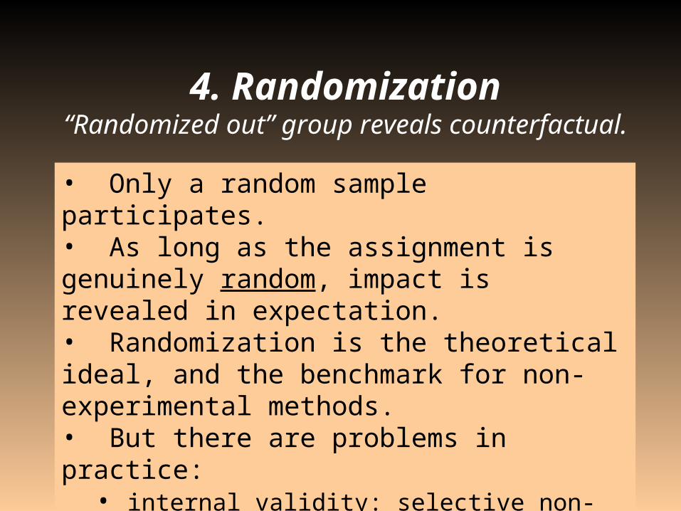
• Only a random sample participates. • As long as the assignment is genuinely random, impact is revealed in expectation.• Randomization is the theoretical ideal, and the benchmark for non-experimental methods. • But there are problems in practice:
• internal validity: selective non-compliance• external validity: difficult to extrapolate results from a pilot experiment to the whole population
4. Randomization“Randomized out” group reveals counterfactual.
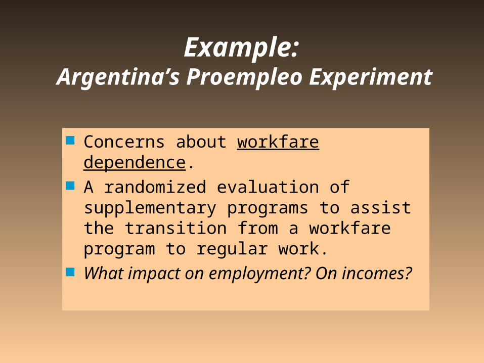
Example: Argentina’s Proempleo
Experiment
Concerns about workfare dependence. A randomized evaluation of
supplementary programs to assist the transition from a workfare program to regular work.
What impact on employment? On incomes?
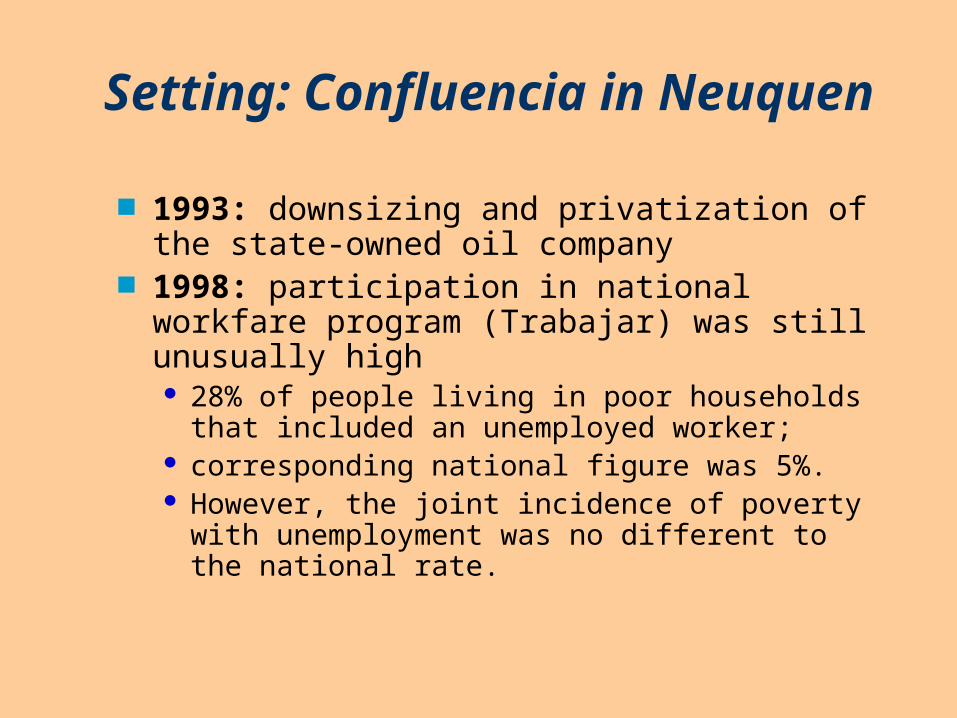
Setting: Confluencia in Neuquen
1993: downsizing and privatization of the state-owned oil company
1998: participation in national workfare program (Trabajar) was still unusually high 28% of people living in poor households that
included an unemployed worker; corresponding national figure was 5%. However, the joint incidence of poverty with
unemployment was no different to the national rate.
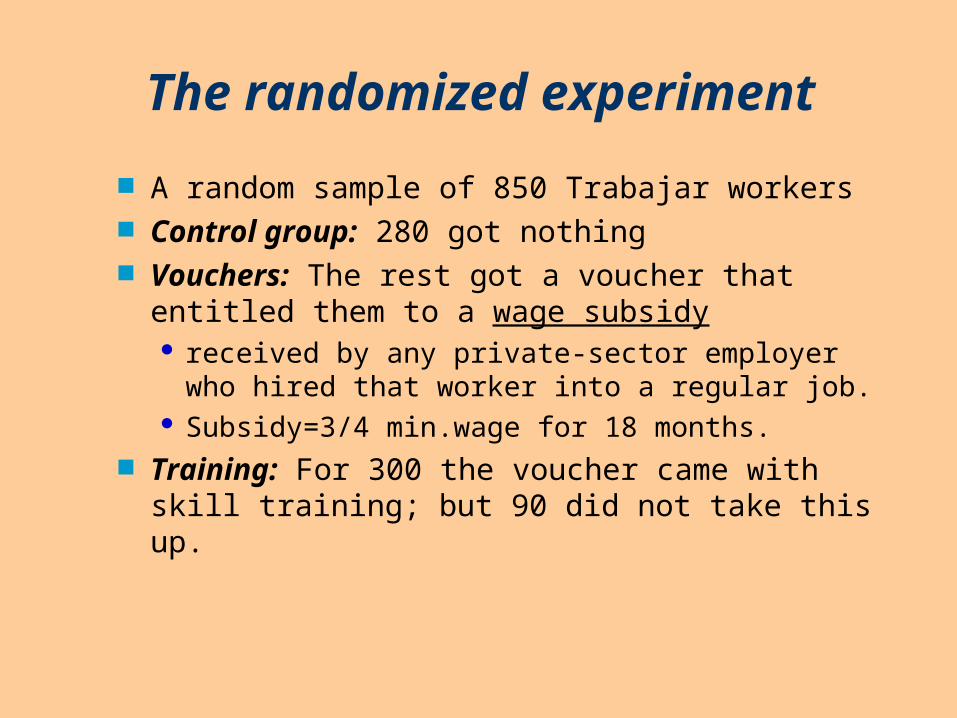
The randomized experiment A random sample of 850 Trabajar workers Control group: 280 got nothing Vouchers: The rest got a voucher that
entitled them to a wage subsidy received by any private-sector employer who
hired that worker into a regular job. Subsidy=3/4 min.wage for 18 months.
Training: For 300 the voucher came with skill training; but 90 did not take this up.

Data for the experiment
Baseline survey by the Statistics Office Three follow-up surveys of all sampled
workers at six month intervals, spanning 18 months.
Experiment was kept secret Different groups visit labor office on different days Local labor office does not know that it is an
experiment
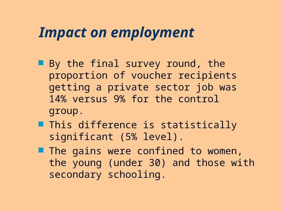
Impact on employment
By the final survey round, the proportion of voucher recipients getting a private sector job was 14% versus 9% for the control group.
This difference is statistically significant (5% level).
The gains were confined to women, the young (under 30) and those with secondary schooling.
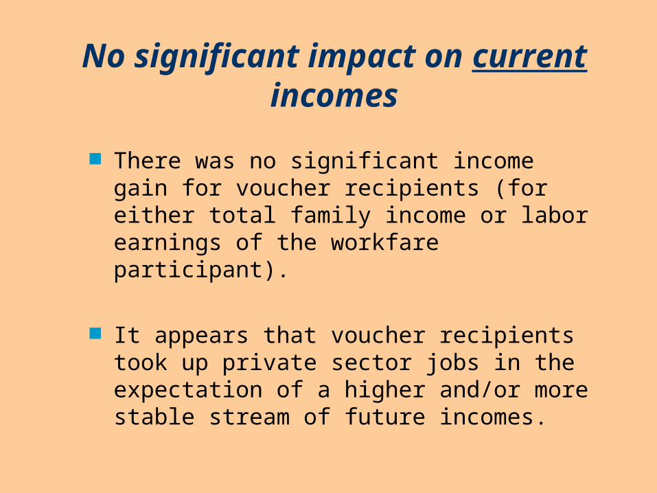
No significant impact on current incomes
There was no significant income gain for voucher recipients (for either total family income or labor earnings of the workfare participant).
It appears that voucher recipients took up private sector jobs in the expectation of a higher and/or more stable stream of future incomes.
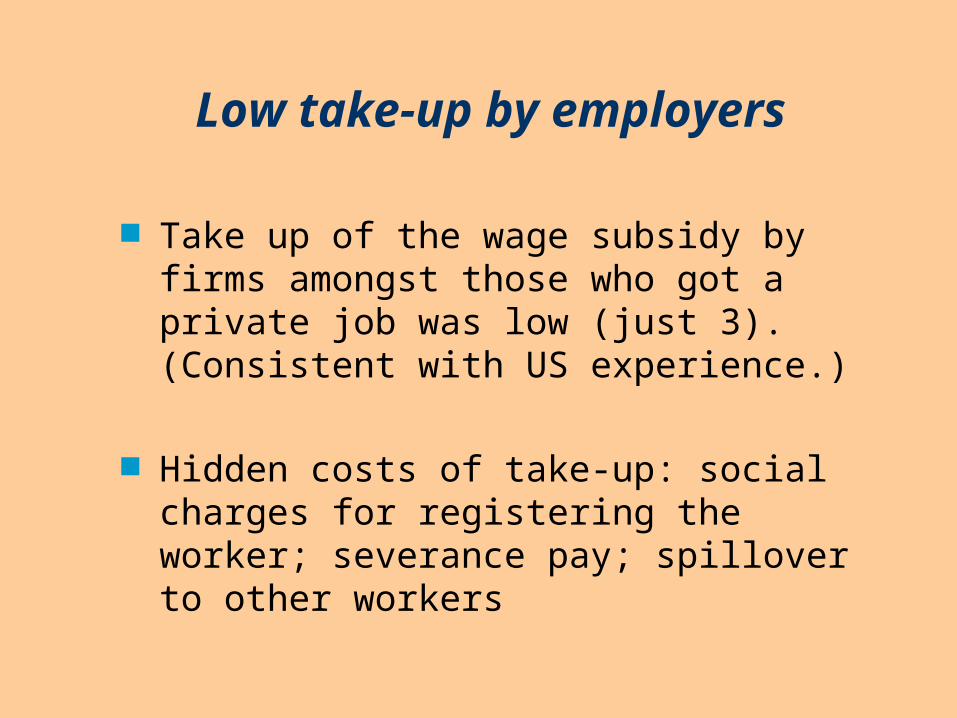
Low take-up by employers
Take up of the wage subsidy by firms amongst those who got a private job was low (just 3). (Consistent with US experience.)
Hidden costs of take-up: social charges for registering the worker; severance pay; spillover to other workers
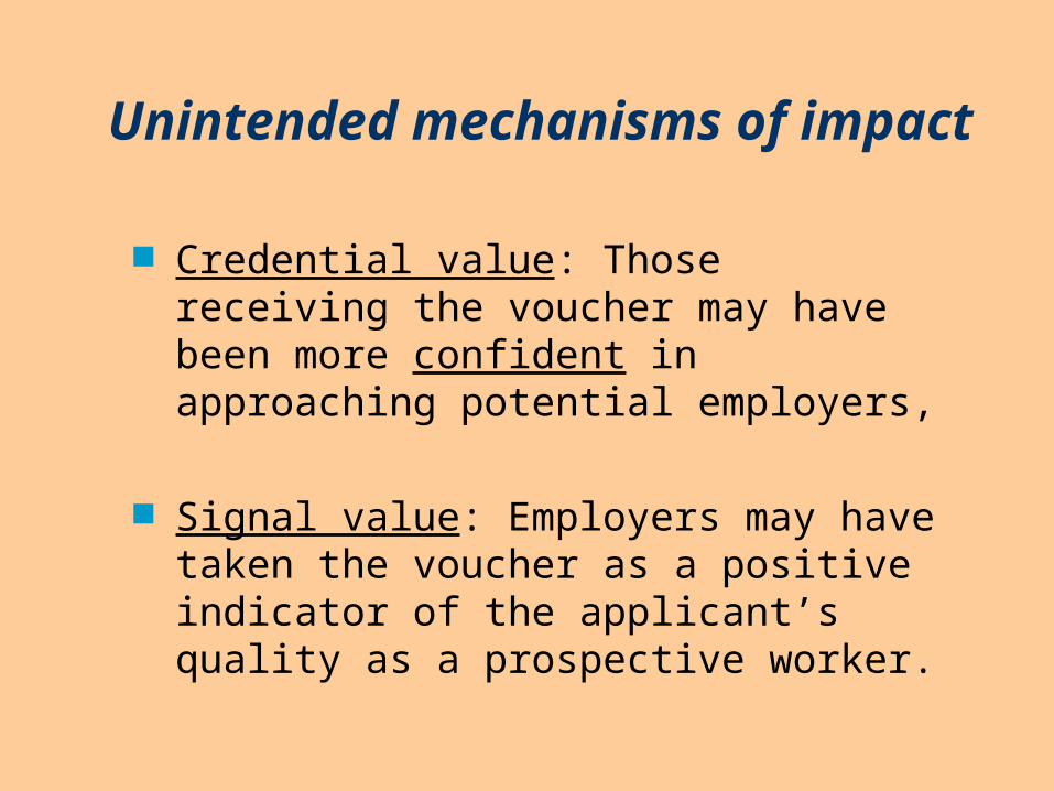
Unintended mechanisms of impact
Credential value: Those receiving the voucher may have been more confident in approaching potential employers,
Signal value: Employers may have taken the voucher as a positive indicator of the applicant’s quality as a prospective worker.
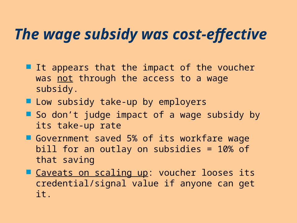
The wage subsidy was cost-effective
It appears that the impact of the voucher was not through the access to a wage subsidy.
Low subsidy take-up by employers So don’t judge impact of a wage subsidy by its
take-up rate Government saved 5% of its workfare wage bill
for an outlay on subsidies = 10% of that saving Caveats on scaling up: voucher looses its
credential/signal value if anyone can get it.
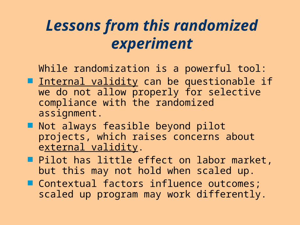
Lessons from this randomized experiment
While randomization is a powerful tool: Internal validity can be questionable if we do not
allow properly for selective compliance with the randomized assignment.
Not always feasible beyond pilot projects, which raises concerns about external validity.
Pilot has little effect on labor market, but this may not hold when scaled up.
Contextual factors influence outcomes; scaled up program may work differently.
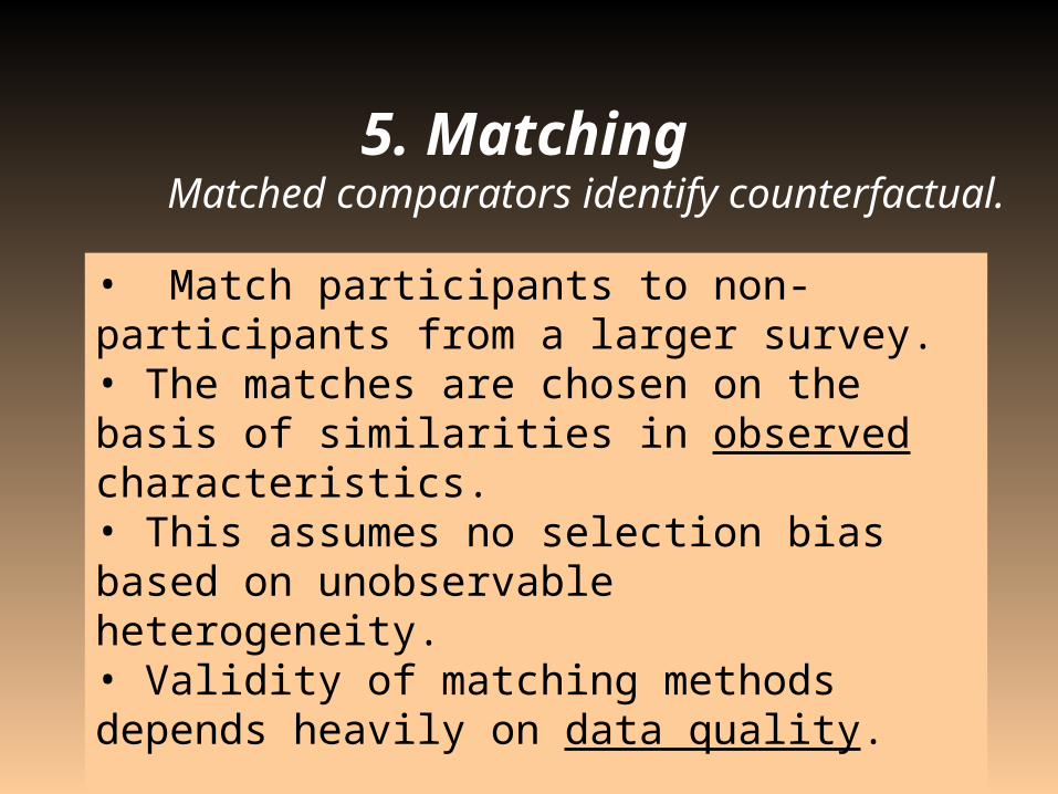
• Match participants to non-participants from a larger survey. • The matches are chosen on the basis of similarities in observed characteristics. • This assumes no selection bias based on unobservable heterogeneity.• Validity of matching methods depends heavily on data quality.
5. Matching Matched comparators identify counterfactual.
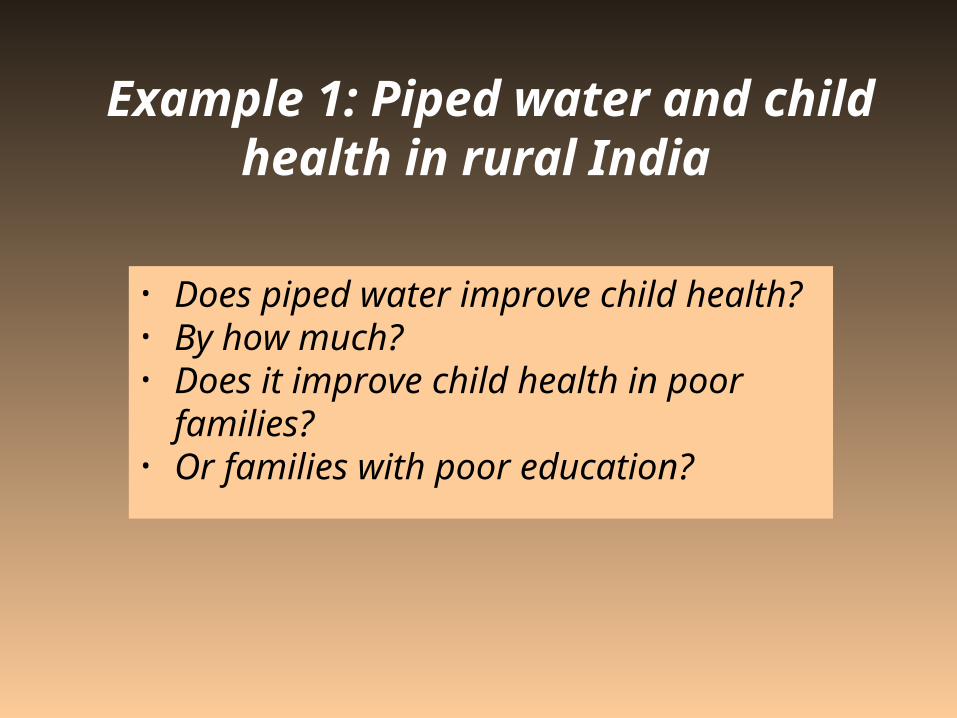
Example 1: Piped water and child health in rural India
• Does piped water improve child health? • By how much?• Does it improve child health in poor
families? • Or families with poor education?
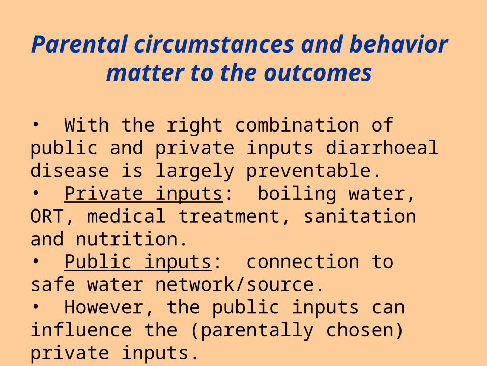
Parental circumstances and behavior matter to the
outcomes
• With the right combination of public and private inputs diarrhoeal disease is largely preventable. • Private inputs: boiling water, ORT, medical treatment, sanitation and nutrition. • Public inputs: connection to safe water network/source.• However, the public inputs can influence the (parentally chosen) private inputs.
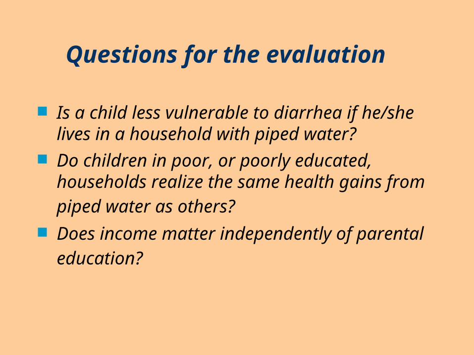
Questions for the evaluation
Is a child less vulnerable to diarrhea if he/she lives in a household with piped water?
Do children in poor, or poorly educated, households realize the same health gains from piped water as others?
Does income matter independently of parental education?
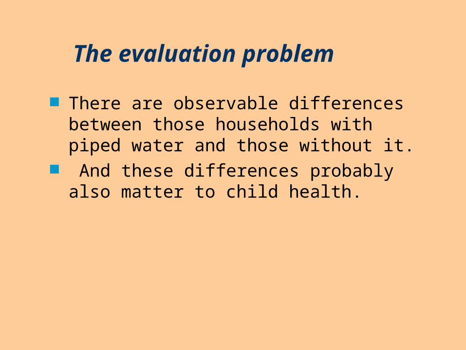
The evaluation problem
There are observable differences between those households with piped water and those without it.
And these differences probably also matter to child health.
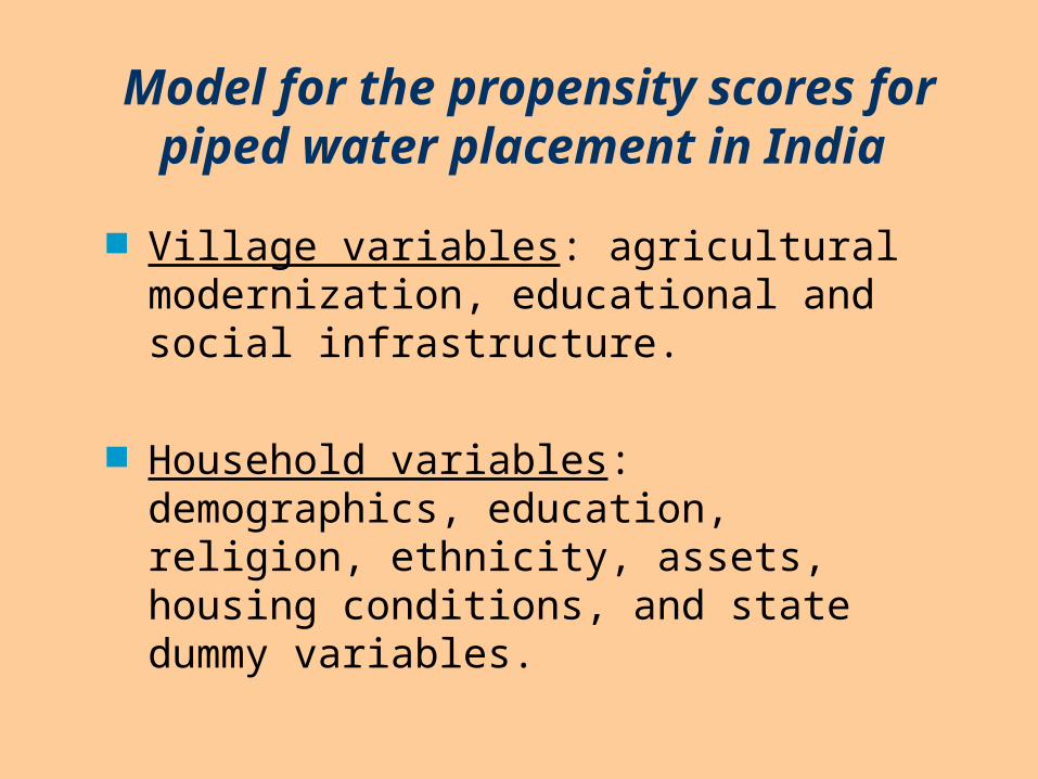
Model for the propensity scores for piped water
placement in India Village variables: agricultural modernization,
educational and social infrastructure.
Household variables: demographics, education, religion, ethnicity, assets, housing conditions, and state dummy variables.
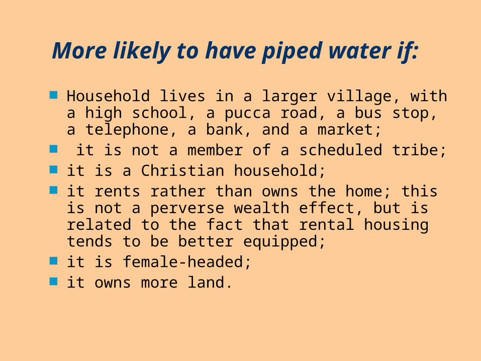
More likely to have piped water if: Household lives in a larger village, with a high
school, a pucca road, a bus stop, a telephone, a bank, and a market;
it is not a member of a scheduled tribe; it is a Christian household; it rents rather than owns the home; this is not a
perverse wealth effect, but is related to the fact that rental housing tends to be better equipped;
it is female-headed; it owns more land.
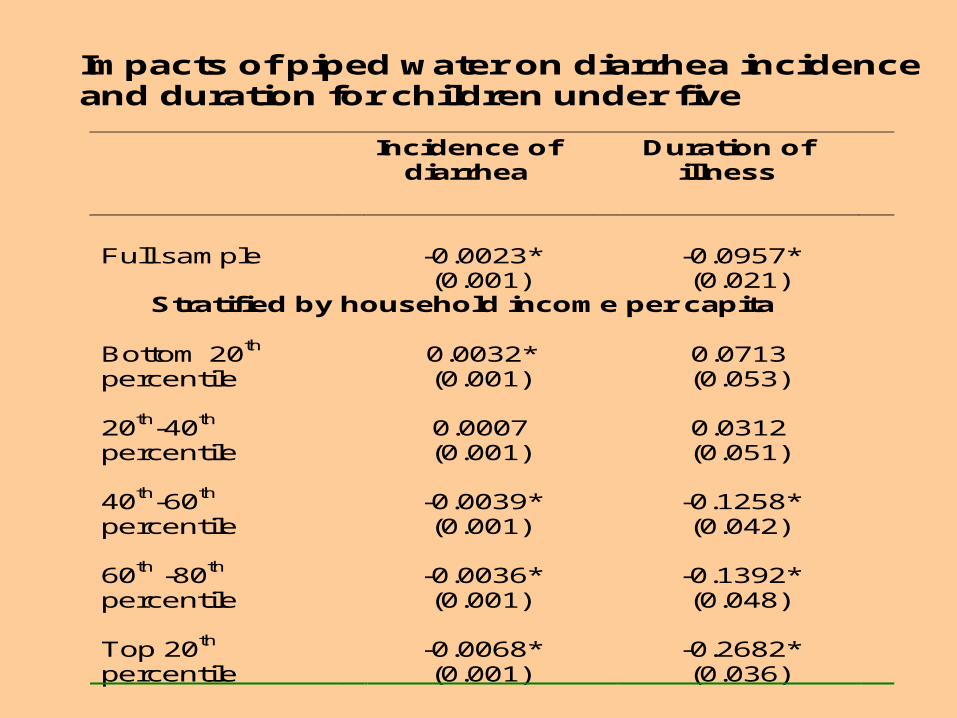
Impacts of piped water on diarrhea incidence and duration for children under five
Incidence of
diarrhea Duration of
illness
Full sample
-0.0023* (0.001)
-0.0957* (0.021)
Stratified by household income per capita Bottom 20th percentile
0.0032* (0.001)
0.0713 (0.053)
20th-40th percentile
0.0007 (0.001)
0.0312 (0.051)
40th-60th percentile
-0.0039* (0.001)
-0.1258* (0.042)
60th -80th percentile
-0.0036* (0.001)
-0.1392* (0.048)
Top 20th percentile
-0.0068* (0.001)
-0.2682* (0.036)
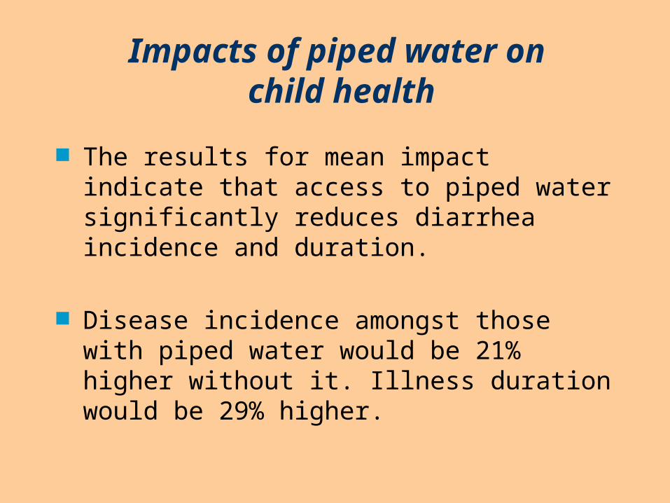
Impacts of piped water on child health
The results for mean impact indicate that access to piped water significantly reduces diarrhea incidence and duration.
Disease incidence amongst those with piped water would be 21% higher without it. Illness duration would be 29% higher.
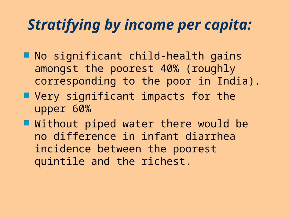
Stratifying by income per capita:
No significant child-health gains amongst the poorest 40% (roughly corresponding to the poor in India).
Very significant impacts for the upper 60% Without piped water there would be no
difference in infant diarrhea incidence between the poorest quintile and the richest.
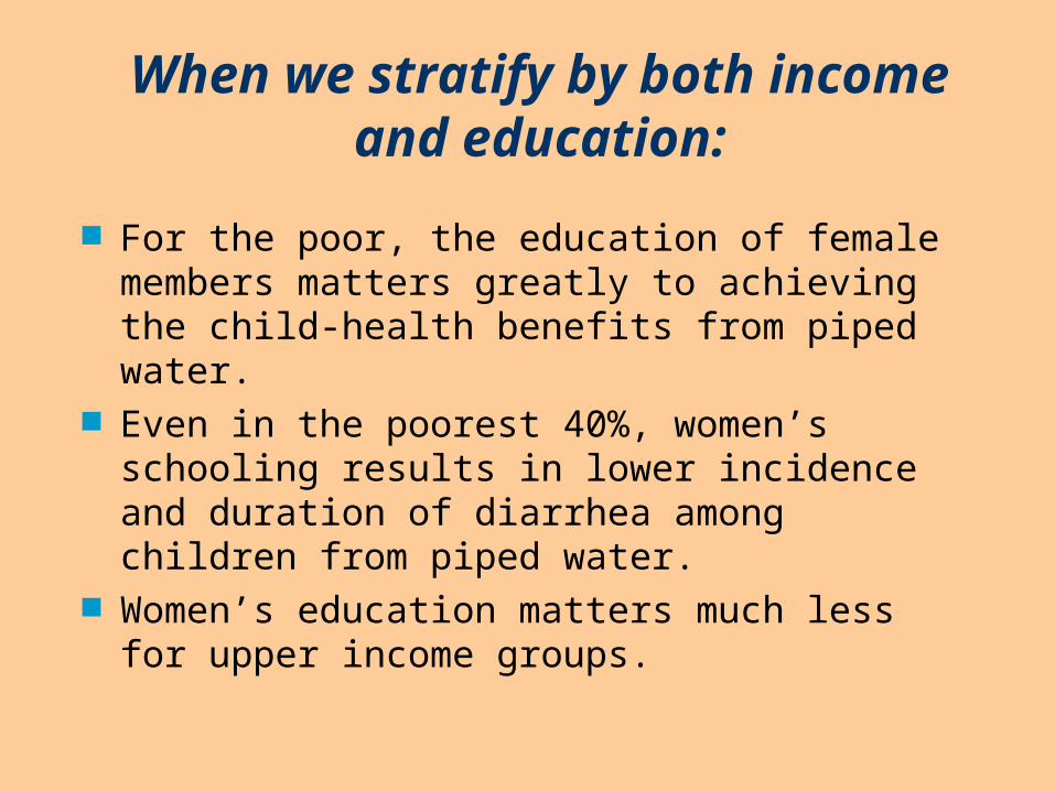
When we stratify by both income and education:
For the poor, the education of female members matters greatly to achieving the child-health benefits from piped water.
Even in the poorest 40%, women’s schooling results in lower incidence and duration of diarrhea among children from piped water.
Women’s education matters much less for upper income groups.

Example 2: A workfare program
in Argentina
Randomization was not an option Nor was it possible to delay the program to
do a baseline survey However, the statistics office (INDEC) had a
survey six months after the program began INDEC and SIEMPRO agreed to add on a
survey of program participants
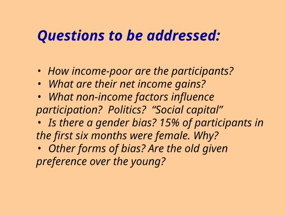
• How income-poor are the participants?• What are their net income gains?• What non-income factors influence participation? Politics? “Social capital” • Is there a gender bias? 15% of participants in the first six months were female. Why?• Other forms of bias? Are the old given preference over the young?
Questions to be addressed:

…. poor, as indicated by housing, neighborhood, schooling, and their subjective perceptions of welfare and expected future prospects …. males who are head of households and married…. longer-term residents of the locality rather than migrants from other areas; …. well-connected: members of political parties and neighborhood associations
The participation regression
Participants are more likely to be:
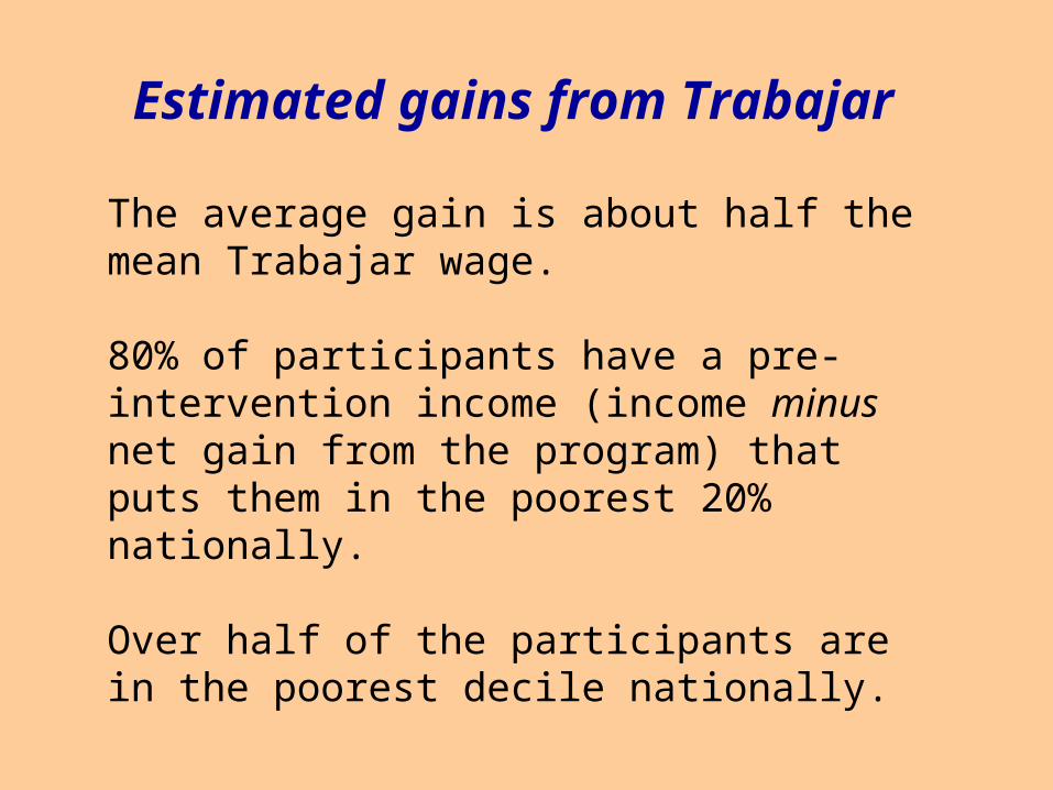
The average gain is about half the mean Trabajar wage.
80% of participants have a pre-intervention income (income minus net gain from the program) that puts them in the poorest 20% nationally.
Over half of the participants are in the poorest decile nationally.
Estimated gains from Trabajar

Standard incidence numbers underestimate how poor the participants would be without the program; over-estimate net gains. This bias is most notable for the poorest 5%• while the non-behavioral analysis suggests that 40% of participants are in the poorest 5%, • the estimate factoring in foregone incomes is much lower at 10%.
Bias in non-behavioral incidence
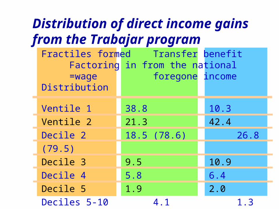
Distribution of direct income gains from the Trabajar programFractiles formed Transfer benefit Factoring in
from the national =wage foregone incomeDistribution
Ventile 1 38.8 10.3
Ventile 2 21.3 42.4
Decile 2 18.5 (78.6) 26.8 (79.5)
Decile 3 9.5 10.9
Decile 4 5.8 6.4
Decile 5 1.9 2.0
Deciles 5-10 4.1 1.3
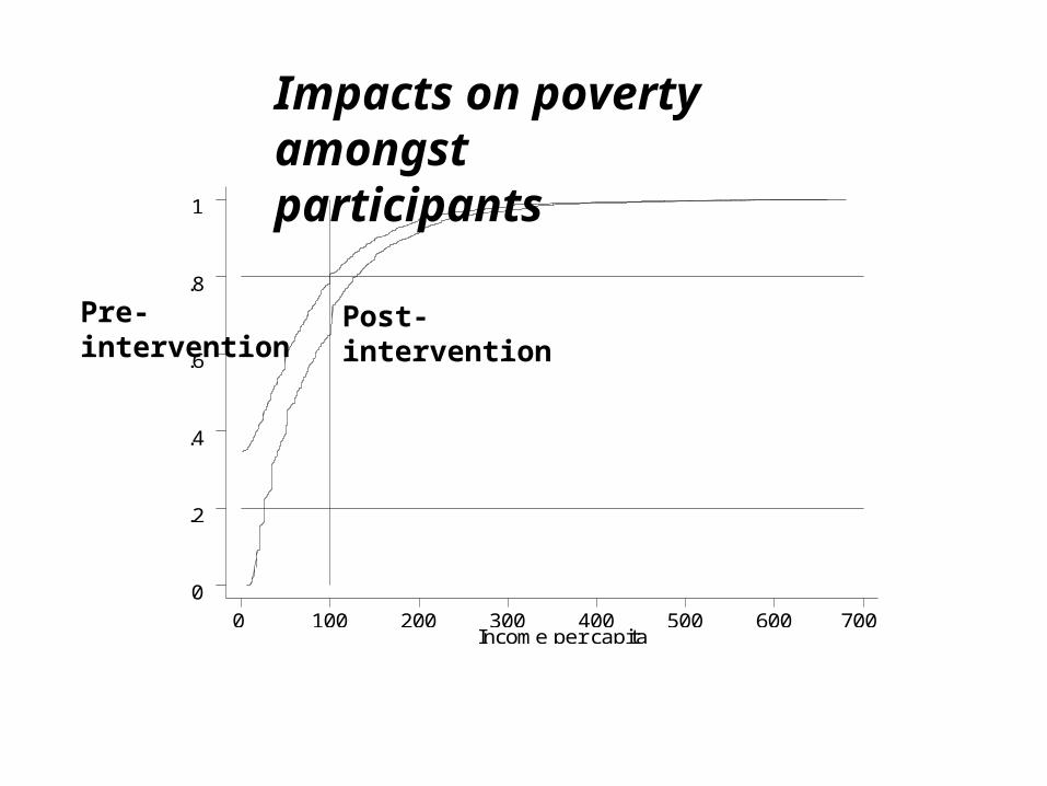
Income per capita 0 100 200 300 400 500 600 700
0
.2
.4
.6
.8
1
Impacts on poverty amongst participants
Pre-intervention Post-intervention
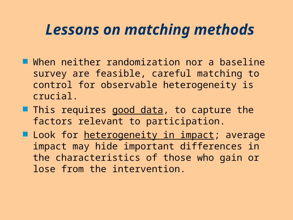
Lessons on matching methods
When neither randomization nor a baseline survey are feasible, careful matching to control for observable heterogeneity is crucial.
This requires good data, to capture the factors relevant to participation.
Look for heterogeneity in impact; average impact may hide important differences in the characteristics of those who gain or lose from the intervention.
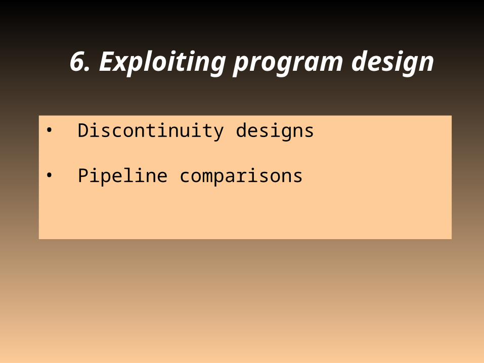
• Discontinuity designs
• Pipeline comparisons
6. Exploiting program design
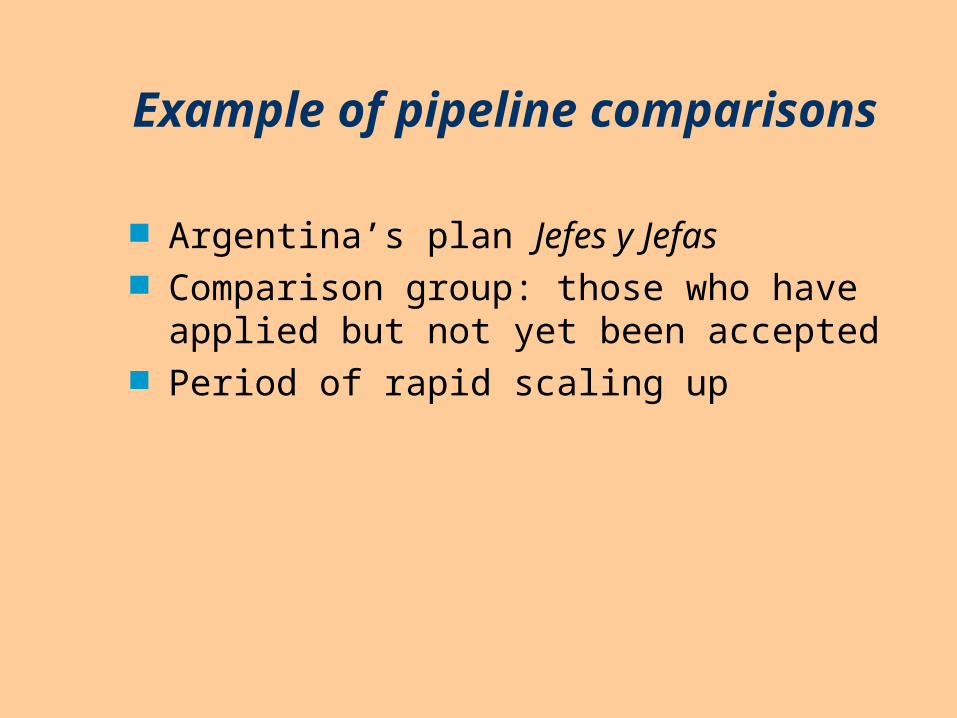
Example of pipeline comparisons
Argentina’s plan Jefes y Jefas Comparison group: those who have applied but
not yet been accepted Period of rapid scaling up
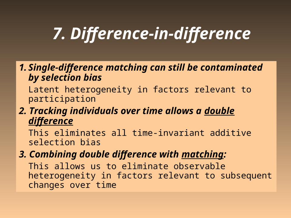
7. Difference-in-difference
1. Single-difference matching can still be contaminated by selection biasLatent heterogeneity in factors relevant to participation
2. Tracking individuals over time allows a double differenceThis eliminates all time-invariant additive selection bias
3. Combining double difference with matching:This allows us to eliminate observable heterogeneity in factors relevant to subsequent changes over time
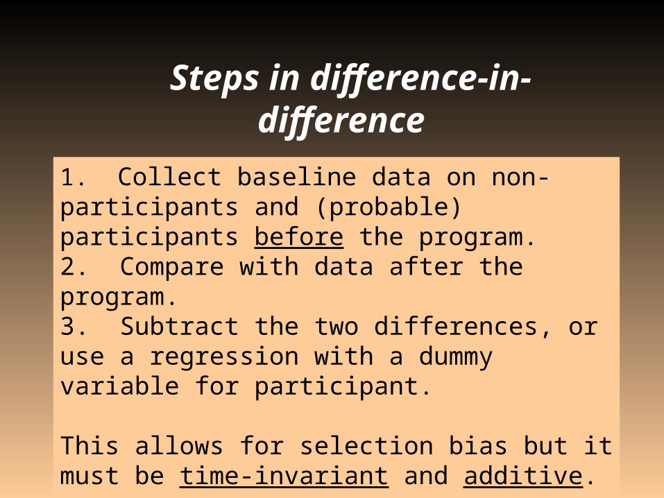
1. Collect baseline data on non-participants and (probable) participants before the program. 2. Compare with data after the program. 3. Subtract the two differences, or use a regression with a dummy variable for participant.
This allows for selection bias but it must be time-invariant and additive.
Steps in difference-in-difference
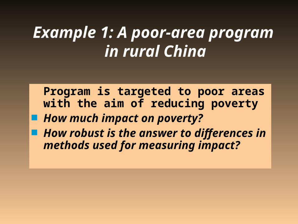
Example 1: A poor-area program
in rural China
Program is targeted to poor areas with the aim of reducing poverty
How much impact on poverty? How robust is the answer to differences
in methods used for measuring impact?
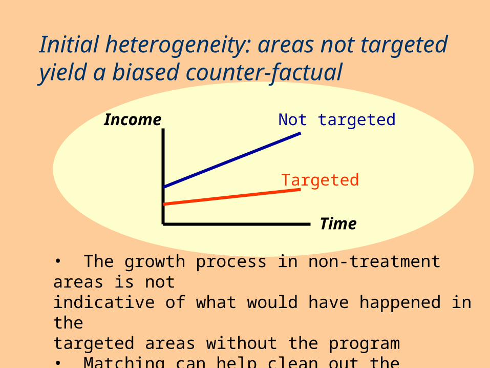
Initial heterogeneity: areas not targeted yield a biased counter-factual
Not targeted
Targeted
Time
Income
• The growth process in non-treatment areas is not indicative of what would have happened in the targeted areas without the program• Matching can help clean out the initial heterogeneity
World Bank’s Southwest Poverty Reduction Project
• Rural development programs targeted to poor areas.• Aims to reduce poverty by providing resources to
poor farm-households and improving social services and rural infrastructure.
• 35 national poor counties • $US400 million over 1995-2001 (from a World Bank
loan and counterpart funding from Chinese government).

Data for the evaluation: Existing survey instrument
Good quality budget and income survey. Sampled households maintain a daily record on
all transactions + log books on production. Local interviewing assistants (resident in the
sampled village, or nearby) visit each household at roughly two weekly intervals.
Inconsistencies found at the local NBS office are checked with the respondents.
Sample frame: all registered agricultural h’holds.
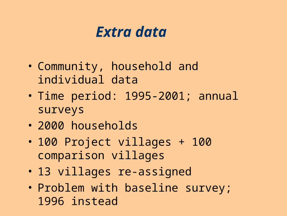
• Community, household and individual data• Time period: 1995-2001; annual surveys• 2000 households• 100 Project villages + 100 comparison
villages• 13 villages re-assigned• Problem with baseline survey; 1996 instead
Extra data
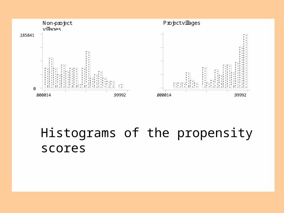
Non project village Project village
Non-project villages
.000014 .99992 0
.185841
Project villages
.000014 .99992
Histograms of the propensity scores
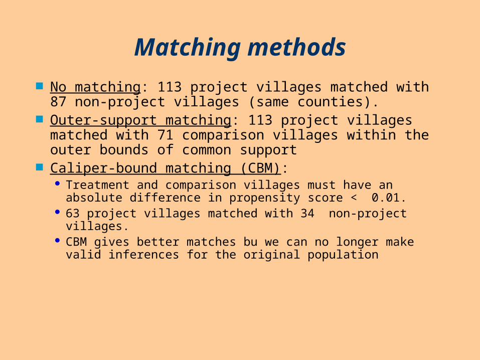
Matching methods
No matching: 113 project villages matched with 87 non-project villages (same counties).
Outer-support matching: 113 project villages matched with 71 comparison villages within the outer bounds of common support
Caliper-bound matching (CBM): Treatment and comparison villages must have an
absolute difference in propensity score < 0.01. 63 project villages matched with 34 non-project villages. CBM gives better matches bu we can no longer make
valid inferences for the original population
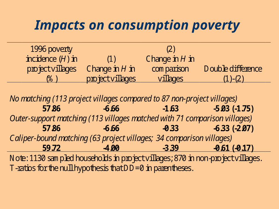
Impacts on consumption poverty
1996 poverty incidence (H) in project villages
(%)
(1) Change in H in project villages
(2) Change in H in
comparison villages
Double difference (1)-(2)
No matching (113 project villages compared to 87 non-project villages) 57.86 -6.66 -1.63 -5.03 (-1.75) Outer-support matching (113 villages matched with 71 comparison villages)
57.86 -6.66 -0.33 -6.33 (-2.07) Caliper-bound matching (63 project villages; 34 comparison villages)
59.72 -4.00 -3.39 -0.61 (-0.17) Note: 1130 sampled households in project villages; 870 in non-project villages. T-ratios for the null hypothesis that DD=0 in parentheses.
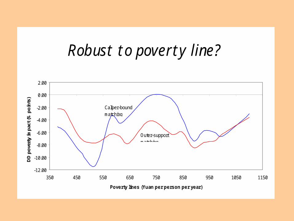
Robust to poverty line?
-12.00
-10.00
-8.00
-6.00
-4.00
-2.00
0.00
2.00
350 450 550 650 750 850 950 1050 1150
Poverty lines (Yuan per person per year)
DD
po
vert
y im
pac
t (%
po
ints
)
Outer-support matching
Caliper-bound matching
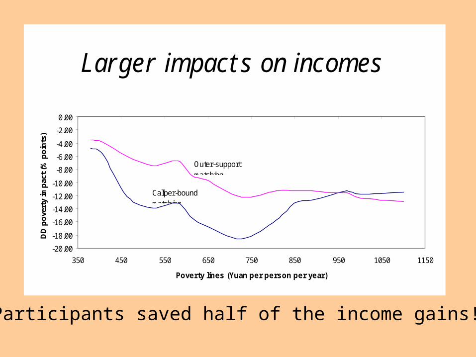
Larger impacts on incomes
-20.00
-18.00
-16.00
-14.00
-12.00
-10.00
-8.00
-6.00
-4.00
-2.00
0.00
350 450 550 650 750 850 950 1050 1150
Poverty lines (Yuan per person per year)
DD
po
vert
y im
pac
t (%
po
ints
)
Outer-support matching
Caliper-bound matching
Participants saved half of the income gains!
Lessons from the SW China evaluation
A large share of the impact on living standards may occur beyond the life of the project. One option: track welfare impacts over much
longer periods; concerns about feasibility. Instead, look at partial intermediate indicators of
longer-term impacts — such as incomes. The choice of such indicators will need to be
informed by an understanding of participants’ behavioral responses to the program, such as based on qualitative research.
8. Higher-order differencing
Example: A workfare program What happens to workfare participants after
they leave the program? Do retrenched workers recover the lost income
from the program? How quickly? What can be learnt about the program’s impact
by tracking leavers and stayers over time?
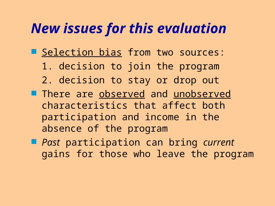
New issues for this evaluation
Selection bias from two sources:
1. decision to join the program
2. decision to stay or drop out There are observed and unobserved
characteristics that affect both participation and income in the absence of the program
Past participation can bring current gains for those who leave the program
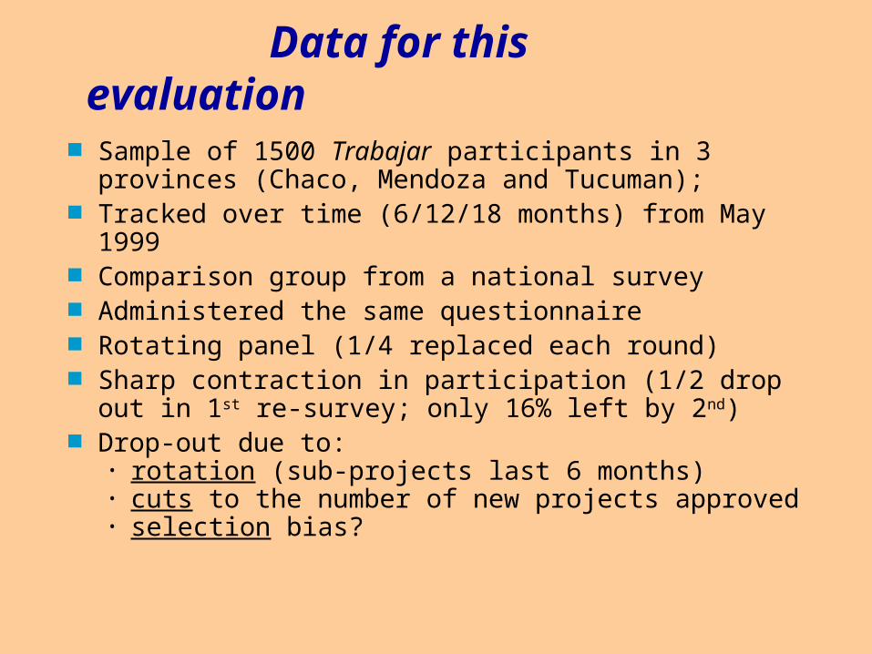
Data for this evaluation
Sample of 1500 Trabajar participants in 3 provinces (Chaco, Mendoza and Tucuman);
Tracked over time (6/12/18 months) from May 1999 Comparison group from a national survey Administered the same questionnaire Rotating panel (1/4 replaced each round) Sharp contraction in participation (1/2 drop out in 1st
re-survey; only 16% left by 2nd) Drop-out due to:
• rotation (sub-projects last 6 months)• cuts to the number of new projects approved• selection bias?
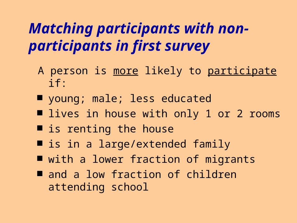
Matching participants with non-participants in first survey
A person is more likely to participate if: young; male; less educated lives in house with only 1 or 2 rooms is renting the house is in a large/extended family with a lower fraction of migrants and a low fraction of children attending school
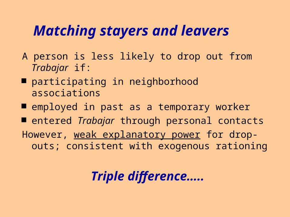
Matching stayers and leavers
A person is less likely to drop out from Trabajar if: participating in neighborhood associations employed in past as a temporary worker entered Trabajar through personal contacts
However, weak explanatory power for drop-outs; consistent with exogenous rationing
Triple difference…..
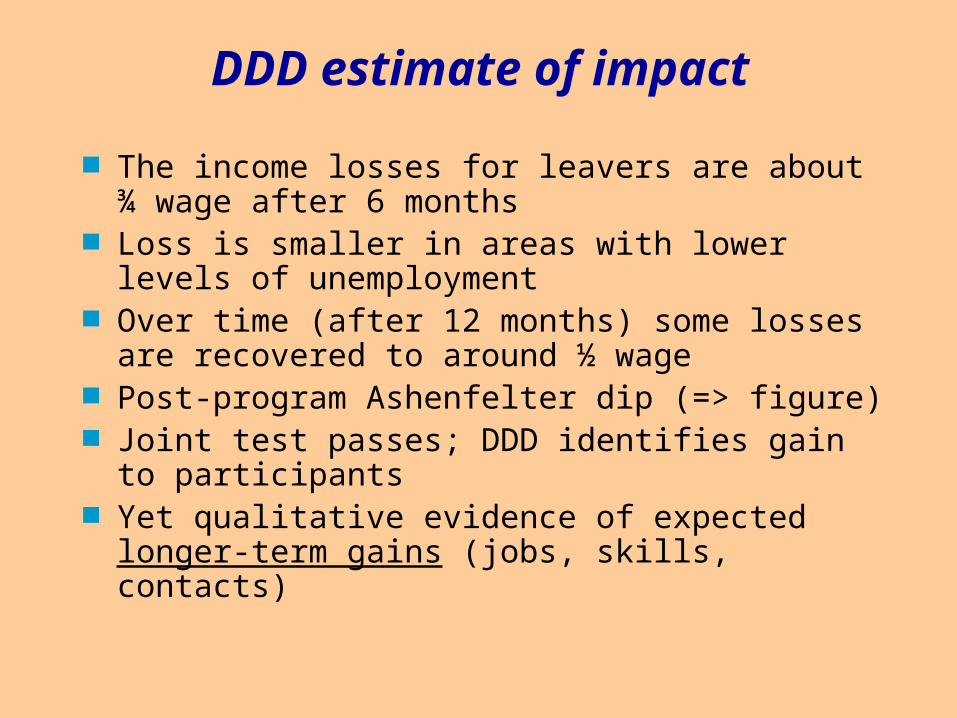
DDD estimate of impact
The income losses for leavers are about ¾ wage after 6 months
Loss is smaller in areas with lower levels of unemployment
Over time (after 12 months) some losses are recovered to around ½ wage
Post-program Ashenfelter dip (=> figure) Joint test passes; DDD identifies gain to
participants Yet qualitative evidence of expected longer-
term gains (jobs, skills, contacts)
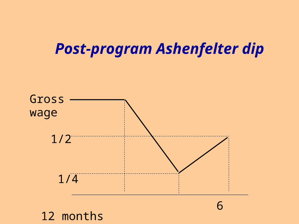
Post-program Ashenfelter dip
Grosswage
1/2 1/4
6 12 months
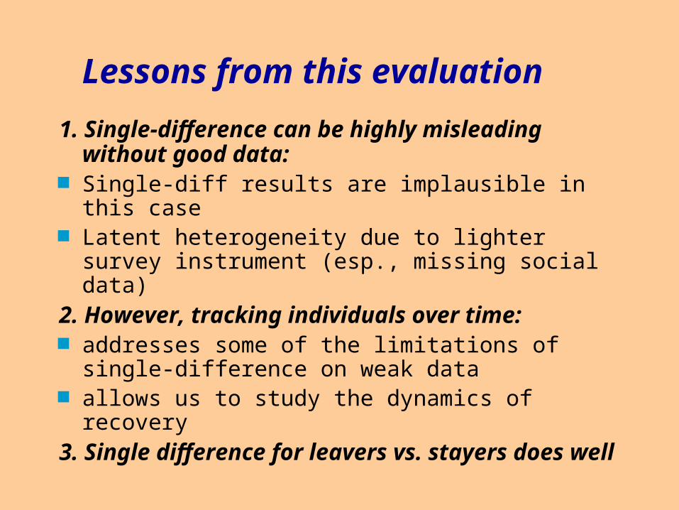
Lessons from this evaluation
1. Single-difference can be highly misleading without good data:
Single-diff results are implausible in this case Latent heterogeneity due to lighter survey
instrument (esp., missing social data)2. However, tracking individuals over time: addresses some of the limitations of single-
difference on weak data allows us to study the dynamics of recovery3. Single difference for leavers vs. stayers
does well
9. Instrumental variablesExample: Proempleo
Experiment
Concerns about workfare dependence. A randomized evaluation of
supplementary programs to assist the transition from a workfare program to regular work.
What impact on employment? On incomes?
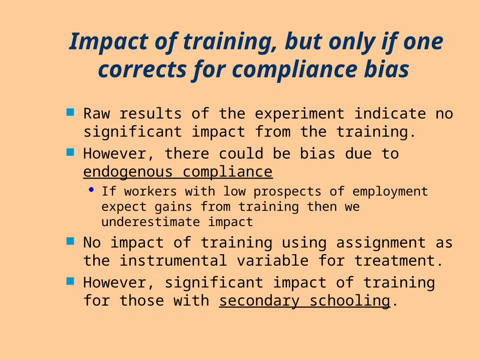
Impact of training, but only if one corrects for compliance
bias Raw results of the experiment indicate no
significant impact from the training. However, there could be bias due to
endogenous compliance If workers with low prospects of employment expect
gains from training then we underestimate impact
No impact of training using assignment as the instrumental variable for treatment.
However, significant impact of training for those with secondary schooling.
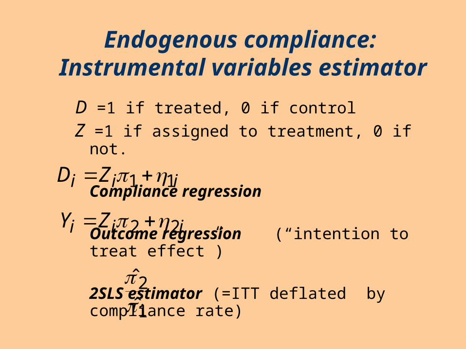
Endogenous compliance: Instrumental variables estimator
D =1 if treated, 0 if control
Z =1 if assigned to treatment, 0 if not.
Compliance regression
Outcome regression (“intention to treat effect”)
2SLS estimator (=ITT deflated by compliance rate)
iii ZD 11
iii ZY 22
1
2ˆˆ


