General rights Copyright and moral rights for the publications made accessible in the public portal are retained by the authors and/or other copyright owners and it is a condition of accessing publications that users recognise and abide by the legal requirements associated with these rights. Users may download and print one copy of any publication from the public portal for the purpose of private study or research. You may not further distribute the material or use it for any profit-making activity or commercial gain You may freely distribute the URL identifying the publication in the public portal If you believe that this document breaches copyright please contact us providing details, and we will remove access to the work immediately and investigate your claim. Downloaded from orbit.dtu.dk on: Jan 18, 2022 Evaluating GRACE mass change time series for the antarctic and Greenland ice sheet- methods and results Groh, Andreas; Horwath, Martin; Horvath, Alexander; Meister, Rakia; Sørensen, Louise Sandberg; Barletta, Valentina R.; Forsberg, René; Wouters, Bert; Ditmar, Pavel; Ran, Jiangjun Total number of authors: 17 Published in: Geosciences Link to article, DOI: 10.3390/geosciences9100415 Publication date: 2019 Document Version Publisher's PDF, also known as Version of record Link back to DTU Orbit Citation (APA): Groh, A., Horwath, M., Horvath, A., Meister, R., Sørensen, L. S., Barletta, V. R., Forsberg, R., Wouters, B., Ditmar, P., Ran, J., Klees, R., Su, X., Shang, K., Guo, J., Shum, C. K., Schrama, E., & Shepherd, A. (2019). Evaluating GRACE mass change time series for the antarctic and Greenland ice sheet-methods and results. Geosciences, 9(10), [415]. https://doi.org/10.3390/geosciences9100415
Transcript
General rights Copyright and moral rights for the publications made accessible in the public portal are retained by the authors and/or other copyright owners and it is a condition of accessing publications that users recognise and abide by the legal requirements associated with these rights.
Users may download and print one copy of any publication from the public portal for the purpose of private study or research.
You may not further distribute the material or use it for any profit-making activity or commercial gain
You may freely distribute the URL identifying the publication in the public portal If you believe that this document breaches copyright please contact us providing details, and we will remove access to the work immediately and investigate your claim.
Downloaded from orbit.dtu.dk on: Jan 18, 2022
Evaluating GRACE mass change time series for the antarctic and Greenland ice sheet-methods and results
Groh, Andreas; Horwath, Martin; Horvath, Alexander; Meister, Rakia; Sørensen, Louise Sandberg;Barletta, Valentina R.; Forsberg, René; Wouters, Bert; Ditmar, Pavel; Ran, JiangjunTotal number of authors:17
Published in:Geosciences
Link to article, DOI:10.3390/geosciences9100415
Publication date:2019
Document VersionPublisher's PDF, also known as Version of record
Link back to DTU Orbit
Citation (APA):Groh, A., Horwath, M., Horvath, A., Meister, R., Sørensen, L. S., Barletta, V. R., Forsberg, R., Wouters, B.,Ditmar, P., Ran, J., Klees, R., Su, X., Shang, K., Guo, J., Shum, C. K., Schrama, E., & Shepherd, A. (2019).Evaluating GRACE mass change time series for the antarctic and Greenland ice sheet-methods and results.Geosciences, 9(10), [415]. https://doi.org/10.3390/geosciences9100415
Evaluating GRACE Mass Change Time Series for theAntarctic and Greenland Ice Sheet—Methodsand Results
Andreas Groh 1,∗ , Martin Horwath 1 , Alexander Horvath 2 , Rakia Meister 3 ,Louise Sandberg Sørensen 3 , Valentina R. Barletta 3 , René Forsberg 3, Bert Wouters 4,† ,Pavel Ditmar 5 , Jiangjun Ran 5,‡ , Roland Klees 5 , Xiaoli Su 6,§ , Kun Shang 6, Junyi Guo 6,C. K. Shum 6,7 , Ernst Schrama 8 and Andrew Shepherd 9
1 Institut für Planetare Geodäsie, Technische Universität Dresden, 01062 Dresden, Germany2 Institut für Astronomische und Physikalische Geodäsie, Technische Universität München,
80333 München, Germany3 DTU Space, Technical University of Denmark, 2800 Kongens Lyngby, Denmark4 Bristol Glaciology Centre, University of Bristol, Bristol BS8 1SS, UK5 Department of Geoscience and Remote Sensing, Delft University of Technology, Stevinweg 1,
2628 CN Delft, The Netherlands6 School of Earth Sciences, The Ohio State University, Columbus, OH 43210-1398, USA7 Institute of Geodesy & Geophysics, Chinese Academy of Sciences, Wuhan 430077, China8 Department of Space Engineering, Delft University of Technology, Kluyverweg 1,
2629 HS Delft, The Netherlands9 Centre for Polar Observation and Modelling, School of Earth and Environment, University of Leeds,
Leeds LS2 9JT, UK* Correspondence: [email protected]; Tel.: +49-351-463-33416† Current address: Institute for Marine and Atmospheric Research, Utrecht University, P.O. Box 80.005,
3508 TA Utrecht, The Netherlands and Department of Geoscience and Remote Sensing, Delft University ofTechnology, Stevinweg 1, 2628 CN Delft, The Netherlands.
‡ Current address: Department of Earth and Space Sciences, Southern University of Science and Technology,Shenzhen 518055, China.
§ Current address: Institute of Geophysics and PGMF, School of Physics, Huazhong University of Science andTechnology, Wuhan 430074, China.
Received: 14 August 2019; Accepted: 17 September 2019; Published: 25 September 2019�����������������
Abstract: Satellite gravimetry data acquired by the Gravity Recovery and Climate Experiment (GRACE)allows to derive the temporal evolution in ice mass for both the Antarctic Ice Sheet (AIS) and theGreenland Ice Sheet (GIS). Various algorithms have been used in a wide range of studies to generateGravimetric Mass Balance (GMB) products. Results from different studies may be affected by substantialdifferences in the processing, including the applied algorithm, the utilised background models andthe time period under consideration. This study gives a detailed description of an assessment of theperformance of GMB algorithms using actual GRACE monthly solutions for a prescribed period as wellas synthetic data sets. The inter-comparison exercise was conducted in the scope of the European SpaceAgency’s Climate Change Initiative (CCI) project for the AIS and GIS, and was, for the first time, open toeveryone. GMB products generated by different groups could be evaluated and directly comparedagainst each other. For the period from 2003-02 to 2013-12, estimated linear trends in ice mass varybetween −99 Gt/yr and −108 Gt/yr for the AIS and between −252 Gt/yr and −274 Gt/yr for the GIS,respectively. The spread between the solutions is larger if smaller drainage basins or gridded GMBproducts are considered. Finally, findings from the exercise formed the basis to select the algorithmsused for the GMB product generation within the AIS and GIS CCI project.
Keywords: GRACE; ice mass change; Greenland; Antarctica; methods
1. Introduction
The Climate Change Initiative (CCI) programme, set up by the European Space Agency (ESA),aims at the provision of reliable, long-term, satellite-based data products to investigate and manageclimate change [1] . Data products are provided for a number of so-called Essential Climate Variables(ECV), which include the Greenland Ice Sheet (GIS) and the Antarctic Ice Sheet (AIS). The Antarctic IceSheet CCI project (AIS_cci) and the Greenland Ice Sheet CCI project (GIS_cci) deliver different ECVparameters for their respective ice sheets, e.g., surface elevation change, ice flow velocity, groundingline location and ice sheet mass balance.
A user survey, performed within a precursor study of the AIS_cci project, indicates that ice sheetmass balance is one of the most important data products required by the scientific community [2].Launched in 2002 and operational until 2017, the Gravity Recovery and Climate Experiment (GRACE)was the only space-borne sensor designed to directly observe mass redistribution [3]. Hence, GRACEsatellite gravimetry data are most suitable to infer mass balance products. Two different types ofGravimetric Mass Balance (GMB) products are provided by the CCI ice sheets projects: (1) time seriesof monthly mass changes for the entire ice sheets and individual drainage basins, describing theevolution in ice mass (GMB basin product), and (2) time series of monthly mass change grids coveringthe entire ice sheet (GMB gridded product), both relative to an arbitrary reference value. Both GMBproducts are described in detail in the corresponding product user guide [4,5].
GRACE Level-2 products include monthly sets of spherical harmonic coefficients of the Earth’sgravity field (Stokes coefficients). They are affected by spatially correlated errors, typically visible interms of north-south orientated stripes in the spatial domain. These error effects require an appropriatepost-processing as a part of GRACE analysis for mass change studies. Proposed filtering approachessuitable to reduce GRACE errors comprise simple isotropic Gaussian filters [6] as well as methodsaccounting for the anisotropic nature of the GRACE errors (e.g., [7,8]). The GRACE error characteristicsimply a limited spatial resolution of 200–500 km, depending on the geographical location, temporalscale, and other factors. Mass changes cannot be resolved with higher spatial resolution due to theattenuation of the corresponding small-scale gravity changes at satellite altitude. This hinders theseparation of nearby mass changes. The resulting error is known as leakage error and may be increasedby the application of a filtering technique [6]. Hence, an algorithm used to derive GMB products needsto efficiently damp GRACE errors while retaining the geophysical signal and reducing signal leakage.
A wide range of studies made use of GRACE-derived time-variable gravity field solutions toinvestigate the spatial and temporal evolution of ice sheet mass. Results from these studies are difficultto compare due to differences in the period under investigation [9], the utilised Level-2 products [10],the model used to correct for solid Earth mass changes (i.e., glacial isostatic adjustment—GIA) [11]and the algorithm applied in the mass change inference. Even in the event of identical input data,differences caused by the algorithms’ ability to reduce both GRACE errors and signal leakage remain.A widely used method makes use of the regional integration approach, which can be equally applied inthe space and the spectral domain [6] and may be combined with an additional leakage correction [12].Other studies make use of so called mass concentrations (mascons), i.e., arbitrarily defined masschange patterns covering small regions of the Earth surface. A finite number of appropriately scaledmascons is used to model the GRACE monthly solutions. Mascon approaches can also be applied inthe spatial [13] and spectral domain [14], while different discretisations have been used (e.g., [15–17]).
To identify the algorithm most suitable for the generation of GMB products for both icesheets, the AIS_cci and the GIS_cci projects jointly performed an open inter-comparison exercise.Participants were asked to derive GMB products from different data sets using their preferredalgorithm. The algorithm evaluation was based on a noise assessment of GRACE-derived GMB
Geosciences 2019, 9, 415 3 of 31
products as well as the quantification of signal leakage by means of simulations with synthetic datasets. The synthetic data sets mimic mass change signals in different compartments of the Earthsystem and are processed using the same algorithm as applied to the GRACE data. By comparingthe results from the synthetic data with the underlying synthetic truth, i.e., the a-priori known masschange of the corresponding data set, the algorithms’ ability to recover the true mass change can beassessed. In addition, the submitted GMB products were compared against each other as well as toindependent data. A comparable assessment of GMB products was part of the broader Ice Sheet MassBalance Inter-comparison Exercise (IMBIE) co-organised by NASA (National Aeronautics and SpaceAdministration) and ESA [18]. IMBIE aimed to produce reconciled ice mass balance estimates for bothAIS and GIS using satellite gravimetry, satellite altimetry and the input-output method. Initiated in2016, IMBIE-2 [19] continued and extended the IMBIE assessment by incorporating a wider rangeof data sets (e.g., GIA models, surface mass balance models) and by being open to a wider range ofscientists. The GMB assessment within IMBIE aimed on basin-scale estimates and was based on theprocessing of GRACE data (IMBIE/IMBIE-2) and a limited set of synthetic data (IMBIE). The presentstudy demonstrates the need for a comprehensive exercise, i.e., the incorporation of an extended set ofsynthetic data and the analyses of both basin and gridded GMB products, for a rigorous assessment ofthe differences between the results derived by various algorithms.
The focus of this study is to describe a methodology, including the required data sets, suitableto perform a thorough assessment of algorithms used for the GMB product generation. Results fromthe product evaluation and inter-comparison are presented and discussed. In this way, the selectionprocess for an algorithm appropriate for the CCI GMB product generation is documented. The paperis structured as follows. In the next section, a detailed description of the exercise setup, including thedata sets to be used (Section 2.2) and the tasks to be fulfilled (Section 2.3) by the participants is given,while Section 2.4 explains the strategy used to assess the submitted GMB products. Section 3 comparesand evaluates the GMB products derived by different algorithms. Finally, Section 4 summarises anddiscusses the results and identifies the algorithms finally used for the GMB production within theAIS_cci and GIS_cci projects.
2. The Inter-Comparison Exercise
2.1. Overview
The inter-comparison exercise was open to everyone. Public announcements on the CCI projectwebsites and through mailing lists of the cryospheric and geodetic community advertised for theexercise. Initially the exercise was designed as a so-called Round Robin Experiment, in whichsets of results are mutually compared. Fully meeting the definition of a Round Robin Experimentrequires a sufficient number of participants as well as a complete set of results from each participantwithout exception.
The results generated within the exercise comprise both GMB basin products and GMB griddedproducts, and are therefore in line with the data sets required from both CCI projects. GMB basinproducts are time series of integrated mass changes over a specific region (e.g., a drainage basin oran entire ice sheet) and are hereinafter given in gigatons (Gt). GMB gridded products indicate masschanges for each cell of a grid covering the whole ice sheet and are given in terms of changes insurface density (i.e., mass per area). They are given in kilograms per meter square or millimetre waterequivalent (mm w.eq., used hereinafter). These products were derived from two different kind ofdata: either GRACE monthly gravity field solutions or synthetic data sets mimicking global massdistributions. While the GRACE-derived products were analysed with respect to temporal changes andthe inherent noise level, results from the synthetic data were used to quantify signal leakage [6] causedby both mass changes of the ice sheets as well as mass changes from surrounding and far-field regions.
In our inter-comparison exercise, synthetic data sets are utilised in the following way. Among otherthings, we want to quantify leakage errors in GRACE-derived estimates of the mean annual mass
Geosciences 2019, 9, 415 4 of 31
change for a certain drainage basin of the ice sheets. For this purpose, a synthetic data set, whichrealistically mimics the spatial pattern of the mean annual mass change over the corresponding icesheet, is required. The data set may stem from geophysical modelling or independent observationslike satellite altimetry, and needs to be available at a spatial resolution better than the actual resolutionprovided by GRACE. For each basin, the true mass change of the synthetic data set (synthetic truth)can be derived by integrating the high-resolution data set over the corresponding basin. If the utiliseddata set is given in the spatial domain, it needs to be converted into GRACE-like data set, i.e., in thespherical harmonic domain with a spatial resolution (maximum spherical harmonic degree lmax)comparable to the GRACE monthly solutions. This synthetic data set, which is global in nature anddescribes the mean annual mass change of the particular ice sheet, is processed in the same way as theGRACE data using the participants’ preferred algorithm. The derived GRACE-like estimate for themean annual mass change for the basin under investigation is compared to the synthetic truth for thisbasin to conclude on the leakage error. This approach provides an estimate for the total leakage error,while discriminating between leakage-in and leakage-out is not possible.
2.2. Data Sets
The following data sets were required to fulfil the tasks described in Section 2.3:
1. GRACE monthly gravity field solutions for the period from 2003-01 to 2013-122. Model predictions to correct GRACE solutions for glacial isostatic adjustment (GIA)3. A series of synthetic data sets to assess the algorithms’ ability to recover the true mass change
To guarantee the comparability of the results, a range of binding requirements on the utiliseddata sets were imposed. Only results based on GRACE Level-2 spherical harmonic gravity fieldsolutions were considered in the exercise. For this purpose all participants made use of the RL05Level-2 data provided by CSR [20], replaced coefficient C2,0 with the SLR estimate by Cheng et al. [21]and added coefficients of degree one derived using the approach of Swenson et al. [22]. Although allparticipants made use of the same Level-2 product, they were free to chose the maximum sphericalharmonic degree (lmax) considered in their analysis, since we consider this choice an integral part ofthe individual processing strategy.
GRACE monthly solutions had to be corrected for GIA using two available models, provided interms of temporal changes of Stokes coefficients (unit: yr−1). The GIA predictions by A et al. [23], basedon the ICE-5G [24] ice load history, were prescribed for applications to the GIS. In the AIS processing,GIA predictions according to the IJ05_R2 model [25] had to be applied. Hence, two different versionsof GIA-corrected GRACE data had to be used for the generation of the AIS and GIS results. GIAmodels still exhibit large uncertainties. However, assessing the GIA model uncertainties is out of thescope of this studies. By prescribing the two GIA models listed above we just wanted to increase theconsistency between the results with respect to the linear trends.
Signal leakage was quantified by means of synthetic data sets, which realistically mimic sources ofleakage errors in terms of mass changes within different subsystems of the Earth (Table 1). Some datasets are based on predictions from geophysical models, providing perennial time series at monthlyresolution (i.e., data sets 01–06, 08–13, 16–27, Table 1). For computational ease, six exemplary epochs,which are approximately evenly distributed over the model period and are representative for the entirerange of the model predictions, were selected for the leakage assessment. The actual epochs of theselected snapshots are indicated in Table 1. Hence, the 27 synthetic data sets do not constitute a timeseries, but must be considered as individual data sets.
Six data sets describe the spatial variability in Antarctic and Greenland surface mass balance (SMB)based on monthly SMB predictions according to the regional atmospheric climate model RACMO2.3.For the AIS (data sets 01–06), modelled SMB values are given on a regular grid with a resolution of27.5 km (RACMO2.3/ANT27) [26], while the spatial resolution of the model for the GIS (data sets08–13) is 11 km (RACMO2.3/GRIS11) [27]. The monthly SMB time series formed the basis to calculate
Geosciences 2019, 9, 415 5 of 31
cumulative SMB anomalies per grid cell with respect to the mean SMB over a multi-decadal period(AIS: 1979–2014, GIS: 1958–2014). Out of these time series, the spatial patterns of cumulated SMBanomalies from six specific months were selected for the exercise. Data sets 01–06 and 08–13 cover theentire AIS and GIS, respectively.
Altimetry-derived patterns of the linear trend in ice mass were utilised to account for the meanannual ice mass change of both ice sheets. For the AIS (data set 07), the spatial pattern of the lineartrend over the period 2010–2013, derived from observations of the radar altimetry (RA) missionCryoSat-2 [28], was utilised. A spatially varying density mask (Figure 1 in [28]) was used to convertsurface elevation trends to mass trends. Correlated patterns of surface lowering and high ice flowvelocities were used to identify regions of dynamical imbalance, for which the density of ice was usedin the conversion. For all other region, except of the stagnating Kamb Ice Stream, the density of snowwas used. The original data set is given on a polar-stereographic grid with a spatial resolution of5 km. For the GIS (data set 14), the spatial trend pattern, given on a 0.5◦× 0.25◦geographic grid, wasderived from laser altimetry observations between 2003 and 2009 acquired by the ICESat mission [9,29].The density of pure ice was used for the conversion from volume change to mass change. The twodata sets (07, 14) cover the entire AIS and GIS, respectively. Separating mass changes of the glaciersand ice caps of the Canadian Arctic Archipelago (CAA) is of particular importance when studying theGIS. To be able to assess leakage caused by the CAA, a respective synthetic data set was generatedbased on the mass loss estimate of Gardner et al. [30]. This pattern is characterised by a surface densitychange with a constant rate and covers all glaciated regions of the archipelago (data set 15).
To be able to assess far-field leakage caused by continental hydrology, synthetic signals werederived from the WaterGAP Global Hydrology Model 2.1 (WGHM) [31]. For this purpose, six snapshots(data sets 16–21) were selected from the monthly time series of global mass anomalies, with respect tothe mean value of the entire time series, covering the period 2002–2014. The model predictions aregiven on a 0.5◦geographic grid and exclude both AIS and GIS.
Table 1. Individual synthetic data sets utilised to quantify signal leakage. For data sets extracted fromperennial model time series the selected epochs are indicated.
Data Set ID Description
01–06 Six data sets of modelled spatial variability in Antarctic surface mass balance (SMB)Epochs: 1980-01, 1986-10, 1996-01, 2004-08, 2009-02, 2014-08
07 Spatial pattern of the mean annual AIS mass change as observed by satellite altimetry
08–13 Six data sets of modelled spatial variability in Greenland SMBEpochs: 1960-05, 1970-10, 1980-05, 1990-10, 2000-05, 2010-10
14 Spatial pattern of the mean annual GIS mass change as observed by satellite altimetry
15 Spatially uniform mean annual ice mass change over the Canadian Arctic Archipelago
16–21 Six data sets simulating residual global oceanic mass variations (e.g., due to errors in the GRACEde-aliasing products)Epochs: 2002-09, 2005-03, 2006-09, 2009-03, 2010-09, 2013-03
22–27 Six data sets of modelled mass changes in global continental hydrology (excluding AIS and GIS)Epochs: 2004-03, 2005-09, 2007-01, 2009-01, 2010-12, 2011-10
Short-term atmospheric and oceanic mass changes are already subtracted from the GRACEmonthly solutions. However, residual mass changes due to errors in the utilised Atmosphere andOcean De-aliasing Level-1b (AOD1B) product [32] may bias GRACE-derived estimates. Here we solelyaccount for residual changes in ocean bottom pressure, which may cause signal leakage from the oceandomain when studying the ice sheets. Differences between the oceanic de-aliasing products (GADproducts) of RL05 [32] and its precursor (RL04) [33] were used to mimic errors in the current GADproducts. Again, six representative monthly solutions (data sets 22–27) served for the investigation
Geosciences 2019, 9, 415 6 of 31
of oceanic signal leakage. Two of these solutions correspond to the months 2007-01 and 2009-01(synthetic data set 18 and 19, Table 1), for which the GAD RL04 product suffers from a bias in thewind stress calculation [34]. Hence, the corresponding differences between both product versionsare exceptionally large and represent an upper limit for the approximated GAD uncertainty. We alsocompared GAD RL05 to ocean bottom pressure estimates from the independent ECCO model (availableat http://grace.jpl.nasa.gov [35,36]). The differences RL05-ECCO are in the same order of magnitudeas RL05-RL04 differences. Spatial patterns exhibit minor differences mainly in shallow water regionsin mid latitudes. Because of this level of agreement and our interest in a data set covering the entireocean, which is not given for ECCO, we found it appropriate to make use of the RL05-RL04 differences.
Each synthetic data set was provided to the participants as a set of spherical harmonic coefficients(Stokes coefficients) up to degree and order 120. This requires the following pre-processing steps.Except for the GAD products, all synthetic data sets were originally available as surface densitychanges in the spacial domain using different grid definitions and projections. These data weretransformed into the spherical harmonic domain by a spherical harmonic analysis up to degree andorder 360. Prior to the spherical harmonic analysis, a Gaussian low pass filter (σ = 25 km) was appliedin the spatial domain to reduce ringing effects at the edge of the data domains, and the grids weredown-sampled to a global geographic grid with a spatial resolution of 0.5◦. Hence, all synthetic datasets are global, although they solely mimic mass changes in certain subsystems of the Earth. Globalmass conservation was ensured by compensating any excessive masses by adding an oceanic masslayer in a gravitationally consistent way according to the sea-level equation (e.g., [37]). The conversioninto Stokes coefficients considers degree one components of the surface density changes according tothe CF (centre of figure) reference system [38].
2.3. Tasks
The results to be generated within the exercise are similar to the GMB products provided by theCCI projects. The primary products are:
1. GMB basin product: series of mass changes per basin2. GMB gridded product: series of mass-change grids (entire ice sheets)
The products listed above had to be derived from two different kind of data sets, namely,the GRACE monthly solutions for the period from 2003-01 to 2013-12 and the synthetic data (Section 2.2).To infer these results the participants were asked to apply their preferred processing strategy.
Mass change time series per basin needed to be inferred for individual drainage basins of bothice sheets as well as for several basin aggregations (Figure 1). The basins were defined according toZwally et al. [39]. In addition to these basins, the following basin aggregations were taken into account:Antarctic Peninsula (AP), East Antarctica (EAIS), West Antarctica (WAIS), the entire Antarctica IceSheet (AIS) as well as the entire Greenland Ice Sheet (GIS).
Figure 1. Drainage basins of the AIS (left) and the GIS (right) based on the basin definitions ofZwally et al. [39]. The inset illustrates basin aggregations for the AIS: Antarctic Peninsula (AP), EastAntarctica (EAIS) and West Antarctica (WAIS).
The gridded GMB product consists of one mass-change grid per epoch solely covering the icesheet. These grids are defined in a polar-stereographic projection with a formal spatial resolution of50 km × 50 km. Hence, gridded results had to be provided using the same grid domain and projection.Since the gridded results were only evaluated over the ice sheets, a well-performing algorithm needsto effectively restore leaked-out signal back to the ice sheet.
Mass changes per basin and mass-change grids also had to be derived from the 27 individualsynthetic data sets. Therefore, each synthetic data set had to be treated in the same way as the series ofGRACE monthly solutions. Of course, replacing C2,0, adding degree one coefficients and applyingcorrections for GIA was not necessary when processing the synthetic data.
2.4. Assessment of Results
Ideally, an appropriate algorithm for the generation of GRACE-derived mass change productsneeds to minimise both GRACE error effects (i.e., the noise) and leakage errors. To validate how thistrade-off was realised by the different approaches applied in the exercise, the assessment comprisesthe following steps:
(A) Visual inspection of the mass change time series(B) Comparison with independent data sets (if possible)(C) Quantification of the temporal changes(D) Quantification of the noise level(E) Comparison of the synthetic results and the underlying synthetic truth
(A) Visual inspection of the mass change time series
A visual inter-comparison of the different results was used to get a first impression of thelevel of agreement. Obvious difference both in signal content and noise level could be identified.The quantification of the revealed differences took place in the subsequent steps of the assessment.
(B) Comparison with independent data sets
An ideal validation data set consists of an independent observation of changes in ice mass, carriedout by an alternative sensor. This sensor needs to be more precise and provide an identical spatialcoverage at higher spatial resolution. Hence, a data set with a temporal resolution of one month and aspatial resolution better than 50 km, covering the entire AIS, is be required. However, no sensor except
Geosciences 2019, 9, 415 8 of 31
of GRACE is able to directly observe changes in mass with a comparable or even better spatial andtemporal coverage. Therefore, observations of alternative quantities related to mass changes have to beused after applying an appropriate conversion. For example, changes in the ice sheet’s surface elevationcan be converted into mass changes using an assumption of the density. A comprehensive overview ofdifferent approaches suitable for determining ice mass changes is given by Shepherd et al. [18].
Only a few independent data sets, fulfilling the requirements listed above, are available. We madeuse of an updated elevation time series derived from several radar altimetry (RA) satellites originallycompiled by Shepherd et al. [18]. As described in Section 2.2, the volume-mass-conversion wasperformed using a prescribed density mask which discriminates between regions where fluctuations inelevation occur with the density of snow or ice [28]. Integrated mass change time series are available forEAIS and WAIS. However, because of the limitations of RA (e.g., sampling issues along the steep coastalmargins or errors in the density assumption used for the volume-mass-conversion), this independentdata set cannot provide a true reference value suitable to be used in a rigorous validation.
Due to the limited number of independent data sets available, we considered a wider range ofdata sets for the comparison with the GRACE results derived within the exercise. We included thereconciled mass change time series for EAIS and WAIS from IMBIE-2 [19], which are a combination ofresults from different techniques (satellite gravimetry, satellite altimetry and input-output-method).Moreover, we also made use of alternative GRACE products. First, mass change time series for AP,EAIS, WAIS, AIS and GIS from an additional mascon approach [16] were utilised and are referred to as“Schrama” in the following. Although this approach is consistent with our exercise in the sense that itworks on Level-2 GRACE data and that the treatment of degree one and C2,0 is identical, there is noconsistency with respect to the applied GIA corrections. Second, we made use of three different masconproducts, which are directly derived from GRACE Level-1 data, to generate mass change time series forall drainage basin and aggregations of both AIS and GIS. The mascon products are provided by CSR(RL05 mascons, v01 [40]), JPL (GLO.RL05M_1 v02, CRI v02 [41]) and GSFC (v02.4 [42]). Hereinafter,time series based on these products are referred to as CSR MC, JPL MC and GSFC MC, respectively.Where necessary, we replaced the GIA correction applied by the processing centres with the correctionused in our inter-comparison exercise.
The comparison of the products generated within the exercise with those from independent andalternative data sets is provided and discussed in Section 4.
(C) Quantification of the temporal changes
Temporal changes in mass change time series were quantified by fitting a linear, periodic (1 year,1/2 year, 161 days) and quadratic model,
y(t) = a + bt +3
∑i=1
(ci sin
(2π
Tit)+ di cos
(2π
Tit))
+ et2
2, Ti = 1 yr, 1/2 yr, 161/365.25 yr (1)
with t being the time relative to the middle of the entire observational period, and by applying anequal weight to every month. Hereinafter this model is referred to as the standard model. The periodicterms account for the dominant periods of geophysical signals (annual and semi-annual) and for the161-day alias period caused by errors in the S2 tide correction [43]. The quadratic term accounts for apossible acceleration in the mass change time series. Although alternative models are possible, thismodel was consistently applied to all data sets. We solved for the model parameters and derivedformal errors for each parameter by means of a least squares adjustment.
(D) Quantification of the noise level
The level of temporally uncorrelated noise in the time series was quantified. This noise includesthe errors of the GRACE monthly solutions, but may also include effects of errors in the de-aliasingmodels, e.g., for atmospheric mass variations. In addition to a noise measure derived from the mass
Geosciences 2019, 9, 415 9 of 31
change time series, we also calculated a noise measure from the average surface density (i.e., mass perarea) time series, which accounts for the area of the drainage basin.
The method for quantifying the noise level is illustrated in Figure 2. First, the major long-term andperiodic signal components were removed by means of the already mentioned model. Residuals of thefitted model still contain both error effects and un-modelled mass changes (e.g., inter-annual changes).To remove still present mass signals a high-pass filter based on a Gaussian average (σ = 2.17 months,corresponding to a 6σ filter width of 13 months) was applied in a second step. The remaining highfrequency residuals, which do not account for any low frequency components or biases, were used toassess the noise level. The calculated standard deviation was scaled to account for the fact that part ofthe temporally uncorrelated noise content was dampened by the preceding steps of model reductionand high-pass filtering. The scaling factor (1.35) was derived through simulations with random noisetime series. Hereinafter, we refer to the scaled standard deviation of the noise time series as the noiselevel. The applied approach may overestimate the actual noise level, since the residuals may stillcontain signal. On the other hand, the method ignores possible temporal correlations of the errors inmonthly GRACE solutions.
Figure 2. Procedure for quantifying the noise level in mass change time series. (a) Original mass changetime series of the AIS (black) and the fitted linear, periodic (1 yr, 1/2 yr, 161/365.25 yr) and quadraticmodel (red). (b) Mass change residuals (black), i.e., original mass change minus fitted model. Redline: Low-pass filtered residuals using a Gaussian average (σ = 2.17 months). (c) High-pass filteredresidual, i.e., residuals minus low-pass filtered residuals. The noise assessment is based on the standarddeviation of this time series.
(E) Comparison of the synthetic results and the underlying synthetic truth
Mass change estimates for ice sheet drainage basins and aggregations derived by processing thespherical harmonic coefficients of the 27 synthetic data sets (Table 1) were compared to the true masschanges (synthetic truth) of the underlying original data set. The differences are used as measuresfor the leakage errors of the basin under investigation, induced by the signal which is mimicked bythe corresponding synthetic data set. For all data sets mimicking mass changes outside the ice sheets,i.e., data sets 08–27 in case of the AIS and data sets 01–07,15–27 in case of the GIS, the synthetic truth iszero by definition for any ice sheet basin. The true mass change of all synthetic data sets covering thestudied ice sheet basin or aggregation, i.e., data sets 01–07 in case of the AIS and data sets 08–14 in caseof the GIS, is derived by integrating the original high-resolution gridded input data as described inSection 2.2.
It was intended to perform this inter-comparison for both the basin-averaged and the griddedresults. Because of the limited number of gridded results from the synthetic data sets submitted by theparticipants, the assessment was limited to the synthetic results per drainage basin (Section 3.1).
3. Results
The subsequent subsections present and discuss both basin averaged and gridded results forAIS and GIS separately and follow the assessment outlined in Section 2.4. In addition to the selected
Geosciences 2019, 9, 415 10 of 31
results presented hereinafter, a compilation of the results for all drainage basins and aggregations canbe found in the supplementary material.
3.1. Submissions
After 13 individuals had registered at the exercise website and downloaded the instructionsand data sets, five different groups finally participated in the exercise. The results were provided byresearch groups at University of Bristol, TU Delft, DTU Space Copenhagen, TU Dresden and Ohio StateUniversity. Each contribution is referenced throughout this document using an ID based on the utilisedprocessing approach. All approaches make use of Level-2 spherical harmonic solutions. Three differentmethods were applied in different variants, namely, regional integration approaches (RI), a forwardmodelling technique (FM) and different mass concentration (or mascon) methods (MC). The term“mascon” is manifold and can also be applied to the forward modelling method. However, here wefollowed the notation of the contributing group and denoted the approach as “forward modelling”.
RI1 [44] results were inferred by a regional integration approach in the spherical harmonic domainusing tailored sensitivity kernels. For every basin or even grid cell a kernel was designed using differentconstraints (optimised by means of synthetic data sets) which allow to control signal leakage andthe impact of GRACE errors using empirical error variance-covariance information. RI2 [45,46] useda regional integration approach in the spatial domain based on gridded equivalent water heights.A leakage correction was used to restore mass leaked to the ocean back to the ice sheet. The forwardmodelling approach FM1 [15] prescribes ice mass changes that are uniform within the coastal and theinland part of each basin. In an iterative procedure, the set of prescribed uniform mass changes wasadjusted in order to fit the GRACE-observed changes in equivalent water height until convergence isreached. MC1 [17] made use of a point mass inversion scheme. GRACE-observed gravity disturbancesat satellite altitude are related to point masses evenly distributed on an icosahedron-based grid.A comparable approach was used by MC2 [47,48], where gravity disturbances at satellite altitudewere converted into mass anomalies in the drainage basins. A unique feature of the MC2 approachis data weighting based on the full error variance-covariance information for each monthly solution.This group has provided a second, regularised solution based on the MC2 results. The regularisationconsiders temporal correlation within the mass change time series. This solution is referred to asMC3 [49]. An overview of submissions from each approach is given in Table 2.
Table 2. Spatial coverage of the results contributed by five groups, derived from GRACE data andsynthetic input data. Basin-scale products comprise all prescribed basins and the entire ice sheet(Figure 1).
ID RI1 RI2 FM1 MC1 MC2/MC3
Results from GRACE data
Basin masschanges
AIS, GIS AIS, GIS AIS, GIS AIS, GIS GIS
Grids AIS, GIS AIS, GIS None AIS, GIS None
Results from synthetic input data
Basin masschanges
AIS, GIS None AIS, GIS AIS, GIS None
Grids AIS, GIS None None None None
All groups have submitted GRACE-derived mass change time series per basin for the GIS,while all except one group have submitted basin-averaged GRACE results for the AIS. Three out offive participants provided time series of GRACE-derived gridded mass changes (both for AIS andGIS). The same applies for the basin-averaged results from synthetic data sets. RI1, FM1 and MC1have provided these results for both AIS and GIS. Gridded results from synthetic data were submitted
Geosciences 2019, 9, 415 11 of 31
by a single group (RI1). The absence of synthetic results severely limits the possibilities to thoroughlyassess the retrieval of ice mass signals by the different algorithms.
Not all participating groups were able to adjust their algorithms and processing chains to fulfilthe full range of assigned tasks (e.g., processing of synthetic data) and to follow the prescribed productspecifications (e.g., use the consistent grid definitions) as described in Section 2.3. Consequently,the largest number of results were submitted for the most common type of products used in ice massstudies: basin mass change time series. The number of results for the gridded products and from thesynthetic data sets was clearly smaller. Considering the number of participants and the completenessof the individual submission, it becomes clear that our inter-comparison exercise does not fully meetthe strict definition of a Round Robin Experiment.
A summary on the utilised data sets and applied methods is given in Table 3. Since RI1 decidedto exclude the monthly solution 2003-01 from their time series, all subsequent analysis steps wereperformed for the period common to all submissions, i.e., the period from 2003-02 to 2013-12.
Table 3. Selected details on the data sets and the processing strategy used by each participating group.
(A) Visual inspection of the mass change time series
Figure 3 compares the different mass change time series for AIS, EAIS, WAIS and AP. In addition,time series for single drainage basins in Dronning Maud Land (AIS06) and the Amundsen Sea Sector(AIS21) are shown. All remaining basins are illustrated in Figures S1–S5. Please note the differentscales among the panels. Differences in the temporal evolution as well as in the noise level are clearlyvisible. For some basins, time series provided by RI2 exhibit deviating temporal changes compared tothe other solutions. This applies both to regions experiencing an increase and decrease in ice mass.
Geosciences 2019, 9, 415 12 of 31
Basin AIS06 experienced a mass gain caused by two exceptional large accumulation events in 2009 and2011 [50]. The dynamic mass loss of basin AIS21 observed by RI2 is significantly smaller compared tothe other solutions.
Figure 3. GRACE-derived mass change time series for (a) the entire Antarctic Ice Sheet (AIS), (b) WestAntarctica (WAIS), (c) East Antarctica (EAIS), (d) the Antarctic Peninsula (AP) as well as the drainagebasins (e) AIS06 (part of Dronning Maud Land) and (f) AIS21 (part of the Amundsen Sea Sector).Figure 1 gives an overview of all drainage basins. The colour coding indicates the results from differentgroups (Table 3).
(C) Quantification of the temporal changes
Figure 4 illustrates the temporal variations in mass change time series derived using the standardmodel, i.e., linear trend, acceleration, amplitudes of seasonal (combined annual and semi-annual) and161-day signal. The numerical values of all estimated parameters including their formal errors fromthe least squares adjustment are summarised in Tables S1–S3.
Geosciences 2019, 9, 415 13 of 31
Figure 4. Temporal changes in ice mass for all AIS basins and aggregations, derived using a consistentlinear, periodic (1 yr, 1/2 yr, 161/365.25 yr) and quadratic model for all time series: (a) linear trend,(b) acceleration, (c) seasonal amplitude, (d) 161-day period, including the formal errors from the leastsquares adjustment.
The linear trend estimates and their formal errors are shown in Figure 4a. For the entireAIS, trend estimates from the participants’ time series vary between −99 Gt/yr and −108 Gt/yr.Larger discrepancies can be found at basin scale. The corresponding formal errors cover the rangebetween ±3 Gt/yr and ±4 Gt/yr, and are even smaller for most of the basins and therefore hard toidentify in the plot. For the majority of basins revealing significant loss in ice mass (e.g., in WestAntarctica), the loss rates for RI2 are clearly the lowest. At the same time, RI2 observes the lowestmass gain for basins in East Antarctica. However, since all participants made use of the same GRACEmonthly solutions, background models and corrections, the revealed discrepancies are solely due todifferent methodologies.
Various studies (e.g., [10,51]) have shown that the consideration of deviating input data mayeven lead to larger discrepancies. For the AIS and the period 2005–2015, Blazquez et al. [51] foundthat trends from GRACE solution series provided by the three official processing centres differ upto 4 Gt/yr, although the differences can be about one order of magnitude larger for other processingcentres. We found that the impact of the maximum spherical harmonic degree lmax does not exceed5 Gt/yr, when considering lmax = 90 and lmax = 60 in the method applied by RI1 (Figure S6). On theother hand, trend differences induced by the utilisation of deviating time series for degree one andC2,0 coefficients can be as large as 29 Gt/yr and 7 Gt/yr, respectively [51]. It is noteworthy, that thespread induced by different degree one time series is larger than the total effect caused by the degreeone time series used by the participants. For example, for method RI2, the neglection of degree onewould reduce the AIS mass loss by 19 Gt/yr (Figure S6). By far the largest error in GRACE-based massbalance estimates is caused by uncertainties in recent GIA models [11]. Trends from various modelsdiffer by up to 61 Gt/yr [51].
Geosciences 2019, 9, 415 14 of 31
Figure 4b depicts the co-estimated acceleration terms for all basins and aggregations. The AISestimates range from −11 Gt/yr2 through −13 Gt/yr2 and agree within the range of the correspondingformal errors. The largest positive accelerations (among all basins and aggregations) are evident forEAIS, mainly caused by the already mentioned accumulation events, while an accelerated mass loss isclearly visible in West Antarctica (WAIS). The revealed differences between the linear trends for RI2and the other groups also apply for the inferred accelerations.
The seasonal amplitudes are shown in Figure 4c. While the estimates for different submissionsagree within the range of the formal errors for most of the basins, the seasonal amplitudes for FM1are clearly larger for certain basins (e.g., AIS09, AIS17, EAIS). Seasonal amplitudes for AIS cover therange between 91 Gt and 120 Gt, while formal errors vary between ±15 Gt and ±18 Gt. Figure 4ddepicts the amplitudes of the 161-day aliasing period, which are at the same order of magnitude as theseasonal amplitude for most of the single drainage basins. However, for larger aggregations (e.g., EAIS,WAIS, AIS), the 161-day amplitudes are considerably smaller, while their error estimates exceed theamplitudes themselves.
(D) Quantification of the noise level
Finally, the noise level of each mass change time series was evaluated as described inSection 2.4 (D). The noise standard deviation of the mass change time series for a single drainagebasin is on the level between 3 Gt and 29 Gt and increases for larger basin aggregations (Figure 5a,Tables S1–S3). The noise level derived from the time series of the average surface density (Figure 5b)clearly indicates that basins of small size (e.g., AIS08, AIS24 or AIS27) are most affected by noise. Timeseries provided by RI2 exhibit the lowest overall noise level.
Figure 5. Noise level, given in terms of the scaled standard deviation of the noise time series, for allAIS basins and aggregations, derived from (a) the mass change time series and (b) the time series ofthe average surface density change. Grey bars indicate the ratio between the basin areas and the entireAIS area.
3.2.2. Synthetic Results per Basin
(E) Comparison of the synthetic results and the underlying synthetic truth
Figure 6 illustrates the differences between the results from the synthetic data sets and the truesynthetic mass changes, which are measures for the leakage errors, for the entire AIS, basin AIS21and basin AIS24. Results for all basins are shown in Figures S8–S12. For all data sets with a non-zerotrue mass change, i.e., data sets covering the AIS, the value of the true mass change is indicated at thetop margin.
Geosciences 2019, 9, 415 15 of 31
Figure 6. Differences between mass change estimates derived from different synthetic data sets andthe corresponding true mass change for (a) the AIS as well as drainage basins (b) AIS21 and (c) AIS24.True (non-zero) mass changes are indicated by numbers at the top margin (unit: gigatons). (d) RMS ofthe differences for all drainage basins (AIS01–AIS24, AIS27, AIS28).
For the entire AIS the largest leakage errors are induced by residual oceanic mass changes,followed by variations in Antarctic SMB and continental hydrology. Far-field effect stemming fromthe GIS and CAA are negligible. It should be kept in mind that the maximum leakage is caused fortwo data sets where the residual oceanic mass changes are exceptionally large (Section 2.2). The sizeof the leakage error depends on both the magnitude and the spatial pattern of the underlying signal.For example, for the entire AIS, leakage from AIS SMB is larger than from the AIS annual mass balancepattern (AIS MB), since overall magnitude of the AIS SMB data sets is larger than for the AIS MB dataset, as indicated by the synthetic truths given in Figure 6.
We chose basin AIS21 (Amundsen Sea Sector) as an example since it is dominated by dynamicthinning and therefore allows us to assess the recovery of the mean annual mass change mimickedby data set 7 (AIS MB). Figure 6 depicts that the algorithms underlying both RI1 and FM1 are able torecover the mean annual mass change equally well. While RI1 slightly underestimates the true massloss, FM1 provides a slight overestimation. The differences are 3.3 Gt and −4.8 Gt corresponding to arelative error of about 5% and 7%, respectively. MC1 almost perfectly recovers the true mass change,with the difference being smaller than one tenth of a gigaton, only. The spread between all threeleakage errors for the mean annual mass change is 8.1 Gt. This is still clearly lower than the additionalerror effects on the linear trend described in Section 3.2.1 (C). For comparison, the spread between thethree linear trend estimates derived from the GRACE time series for AIS21 is 3.8 Gt/yr (RI1 being lessnegative than MC1 and FM1). We also found that the different maximum spherical harmonic degreeused by the participants has a minor impact on the corresponding leakage errors (Figure S20).
Basin AIS24 (George VI Sound) is located close to Alexander Island whose changes in surfacemass balance are included in the synthetic data sets 1–6 (AIS SMB). Therefore, the algorithm’s abilityto separate these nearby signals can be studied. Like for other basins, the largest leakage errors are
Geosciences 2019, 9, 415 16 of 31
induced by SMB variability. However, for basin AIS24 the SMB-induced leakage is clearly largercompared to other basins. For example, in comparison to basin AIS21 the leakage error may be abouttwice as large, depending on the magnitude of the SMB signal. For most of the synthetic data sets onSMB variability, FM1 results exhibit the smallest leakage errors for basin AIS24.
For a more comprehensive assessment, we need to consider all drainage basins. Leakage errorsdepend on the magnitude and pattern of the inducing signal, the area of the basin under investigationor, in case of leakage caused by the nearby ocean, on the length of the shoreline. Hence, leakage errorsdiffer between the basins. Figure 6d gives a general overview on the leakage errors showing the rootmean square (RMS) of the differences between the individual synthetic estimates and the synthetictruth for all drainage basins constituting the entire AIS. It becomes evident that leakage inducedby AIS SMB variability is largest, while far-field changes in ice mass (GIS and Canadian Arctic) arenegligible. Leakage caused by errors in the oceanic component of the GRACE de-aliasing product maybe in the same order of magnitude as errors caused by continental hydrology. Hence, basin-averagedmonthly mass change estimates derived from GRACE may exhibit leakage errors in the order of 10 Gt,on average. The large errors for oceanic data sets 18 and 19 are related to gross errors in the de-aliasingproduct and can be considered an upper limit. In general, no coherent differences could be identifiedin the overall performance of RI1 and FM1 for the dominant leakage signals (AIS SMB and Ocean),although RI1 performs slightly better in terms of AIS SMB signal leakage, whereas FM1 performsbest in terms of the Ocean signal leakage. MC1 exhibits slightly larger leakage errors stemming fromsignals in the ocean and continental hydrology.
3.2.3. GRACE-Derived Gridded Mass Changes
The gridded results submitted by the different groups differ with respect to their representation(e.g., regular geographic grid projected to a polar-stereographic plane, regular polar-stereographic gridor an icosahedron grid). For the AIS, three sets of gridded results are available, namely, RI1, RI2 andMC1. These data were used to quantify temporal changes and the noise level for each grid cell asdescribed in Sections 2.4 (C) and (D), respectively. However, this did not allow us to directly comparethe results from different groups. For a quantitative comparison, all but the RI1 results for the lineartrend and the noise level were interpolated to the prescribed polar-stereographic grid with a gridspacing of 50 km× 50 km grid (Section 2.3). In this step we did not extrapolate beyond the domainof the original grids. Hence, all cells of the polar-stereographic grid lying outside the original griddomain were ignored in the comparison.
(C) Quantification of the temporal changes
Figure 7 reveals significant differences between the patterns of the linear trend. Since the lineartrends for the entire AIS are nearly identical for MC1 and RI2 (Figure 4), the same applies for theaverages of the gridded trends (−8.3 and −8.1 mm w.eq./yr). The small difference arises from differingareas covered by the interpolated gridded products. In theory, if two algorithms are comparablyeffective in restoring ice mass changes back to the ice sheet, a smaller solution area would result in alarger change in surface density, both in terms of the average as well as the extreme values. However,existing differences in the extreme values visible in Figure 7 indicate differences in the algorithms’performance. Both the mass loss in West Antarctica and the mass gain, e.g., along coastal regions ofEast Antarctica (Dronning Maud Land), are clearly the weakest for RI2. While the trend for MC1 rangesfrom −678.7 to 208.3 mm w.eq./yr, the trend for RI2 varies between −284.3 and 53.8 mm w.eq./yr,only. The largest average mass loss trend is revealed for RI1 (−8.5 mm w.eq./yr), even though theirextreme values (−562.2 and 185.6 mm w.eq./yr) do not exceed those of MC1. Moreover, RI1 exhibitsfeatures of smaller scale in terms of more localised mass trend patterns (e.g., over the Kamb Ice Stream).The largest differences are revealed between MC1 and RI2, with an RMS of 49.0 mm w.eq./yr, while theRMS of the differences between MC1 and RI1 is 36.8 mm w.eq./yr, only. The RMS difference betweenRI1 and RI2 is 41.7 mm w.eq./yr.
Geosciences 2019, 9, 415 17 of 31
Figure 7. Linear trends derived from the gridded mass changes, using a consistent linear, periodic(1 yr, 1/2 yr, 161/365.25 yr) and quadratic model, and interpolated to the prescribed regularpolar-stereographic grid. Panels (a–c) show results from different groups (Table 3). Grid cells ingrey lie outside of the original grid domains.
(D) Quantification of the noise level
Figure 8 reveals large differences between the noise levels of the gridded products. The largestnoise level was found for RI1 with an RMS of 229.7 mm w.eq. In particular, coastal regions are heavilyaffected by noise, exceeding the 500 mm. w.eq. level. Over the ice sheet artefacts of GRACE stripingpatterns are still visible. The noise level of MC1 (RMS: 92.5 mm w.eq.) is clearly lower than for RI1.However, larger noise along the coastal margins, compared to the interior of the ice sheet, can alsobe observed for MC1. By far the lowest overall noise level is revealed for RI2, which shows onlyminor variations over the AIS, with slightly increased value at the tip of the Antarctic Peninsula(AP). The RMS for RI2 (32.8 mm w.eq.) is about one order of magnitude smaller than for RI1. Hence,the largest differences are found between the noise levels of RI1 and RI2. The RMS of the differencescalculated for all common grid cells is 169 mm w.eq.
Synthetic data sets can help to identify the origin of the larger noise in coastal regions. Figure 6reveals the largest leakage errors for the data sets mimicking residual oceanic mass changes (Table 1).However, these basin-integrated estimates do not allow for an assessment of the spatial patterns.This information can only be derived from gridded results derived from the synthetic data sets,which were solely provided by RI1 (Table 2). We found that gridded leakage errors derived fromsynthetic data sets 16–21 (not shown) can be as large as 500 mm w.eq. along the coastline. The samealso applies to other synthetic data mimicking far-field signals, e.g., from the continental hydrology(data sets 22–27), which also include an oceanic component through the mass conserving ocean layer.
Geosciences 2019, 9, 415 18 of 31
Figure 8. Noise level, given in terms of the scaled standard deviation of the noise time series, estimatedfrom the gridded mass changes. Panels (a–c) show results from different groups (Table 3). Grid cells ingrey lie outside of the original grid domains.
3.3. The Greenland Ice Sheet
3.3.1. GRACE-Derived Mass Changes per Basin
(A) Visual inspection of the mass change time series
Mass change time series for the entire GIS as well as basins GIS01 (northern GIS), GIS03 (eastern)and GIS04 (south-eastern) are compared in Figure 9. Figures for all GIS basins are provided inthe Supplementary Materials (Figures S14 and S15). Note that MC2 has provided an additional,regularised solution referred to as MC3. The most northern basin GIS01 is closest to the CanadianArctic Archipelago and potentially affected by leakage-in. Differences in the temporal evolution andthe noise content are evident for every basin. Time series provided by RI2 reveal the smallest loss inmass for the entire GIS. For basin GIS03 the MC2/MC3 time series clearly deviate from the majorityof time series. While the decrease in ice mass is smaller for basin GIS03 the opposite is true for theneighbouring basin GIS04. This is a clear indication for differences in signal leakage, caused by theneighbouring basins, among the various results. These differences can only be verified by means ofsynthetic data sets.
Geosciences 2019, 9, 415 19 of 31
Figure 9. GRACE-derived mass change time series for (a) the entire Greenland Ice Sheet (GIS) aswell as the drainage basins (b) GIS01 (North Greenland), (c) GIS03 (East Greenland) and (d) GIS04(South-east Greenland). Figure 1 gives an overview of all drainage basins. The colour coding indicatesthe results from different groups (Table 3).
(C) Quantification of the temporal changes
Linear trends derived using the standard model and their corresponding error estimates areshown in Figure 10a. Using the standard model, the consistently inferred linear trends for GIS varybetween −213 Gt/yr and −274 Gt/yr, while the corresponding formal errors of the trends derivedfrom the least squares adjustment are in the range of ±1 Gt/yr. The significant spread between theresults is mainly caused by the RI2 estimate. Excluding this result reduce the range to −252 Gt/yrthrough −274 Gt/yr. Numerical values for all basins are given in Table S4.
As already outlined in the section on the AIS results, different choices of input data may leadto discrepancies in the trends still exceeding the discrepancies revealed here. Blazquez et al. [51]quantified the following variations in linear trend depending on the input data (entire GIS, 2005–2015):GRACE monthly solution series: up to 10 Gt/yr, degree one: 7 Gt/yr, C20: 4 Gt/yr, GIA correction:4 Gt/yr. We assessed the impact of the degree one time series through the example of RI2 and found theimpact on the trend to be 4 Gt/yr. This estimate is in the same or of magnitude as the trend differencesderived by Blazquez et al. [51]. The impact of the maximum spherical harmonic degree (RI1: lmax = 90vs. lmax = 60) is no larger than 1 Gt/yr (Figure S16).
Figure 10b depicts the jointly estimated acceleration terms for all basins and aggregations. The GISestimates range from −21 Gt/yr2 through −30 Gt/yr2, indicating an increased overall mass loss. Thisrange is reduced to −24 Gt/yr2 to −30 Gt/yr2 if the RI2 results is excluded. The largest accelerationscan be observed for the western basins GIS06 and GIS07, where an increased mass loss is observablefrom 2005 onwards.
The seasonal amplitudes shown in Figure 10c vary significantly between 114 Gt and 172 Gtfor the entire GIS, while the corresponding errors are in the range from ±4 Gt to ±7 Gt. RI2 andMC1 exhibit clearly smaller amplitudes for GIS and most of the basins compared to the remaining
Geosciences 2019, 9, 415 20 of 31
submissions. Table S4 reveals that this offset mainly originates from the annual component of theseasonal amplitude. The smaller seasonal signals for RI2 are, in a way, consistent with the smaller massloss rates (Figure 10a). This does not apply for MC1. Somewhat larger amplitudes for FM1 (e.g., basinGIS04) are in agreement with our findings for the AIS. The amplitudes of the 161-day aliasing period(Figure 10c) do not exceed 10 Gt for single drainage basins and agree within the corresponding errorestimates among the different submissions.
Figure 10. Temporal changes in ice mass for all GIS basins and aggregations, derived using a consistentlinear, periodic (1 yr, 1/2 yr, 161/365.25 yr) and quadratic model for all time series: (a) linear trend,(b) acceleration, (c) seasonal amplitude, (d) 161-day period, including the formal errors from the leastsquares adjustment.
(D) Quantification of the noise level
The standard deviations of the noise, assessed according to Section 2.4 (D), are shown in Figure 11a.The noise standard deviation for a single drainage basin time series varies between 4 Gt and 30 Gt,where the noise is higher for larger basin aggregations. The noise level derived from the averagesurface density time series is shown in Figure 11b and reveals that the small basin GIS05, located atthe southern tip of Greenland, is mostly affected by noise. Using basin definitions which avoid verysmall basins like GIS05, e.g., the basin definitions used in IMBIE-2, may help to reduce the noise levelof the corresponding mass change time series. Time series provided by RI2 and MC2/MC3 exhibit thelowest overall noise level. For the entire GIS, the linear trend estimates from these solutions are theleast negative (Figure 10a).
Geosciences 2019, 9, 415 21 of 31
Figure 11. Noise level, given in terms of the scaled standard deviation of the noise time series, for allGIS basins and the entire GIS, derived from (a) the mass change time series and (b) the time series ofthe average surface density change. Grey bars indicate the ratio between the basin areas and the entireGIS area.
3.3.2. Synthetic Results per Basin
(E) Comparison of the synthetic results and the underlying synthetic truth
Figure 12 compares the differences between the results from all synthetic data sets with thecorresponding true mass changes for the entire GIS as well as basins GIS01 and GIS04. Results for allbasins are depicted by Figures S18 and S19. For the entire GIS, the mean annual mass change is wellrecovered by all three approaches (RI1, FM1, MC1). The absolute differences between the synthetictruth of data set 14 (GIS MB) and the user estimates are below 1 Gt for RI1 and MC1, and are about2 Gt for FM1, only. Hence, leakage errors in GRACE-derived mass balance estimates for the entireGIS are supposed to be clearly smaller than additional error effects on the linear trend, e.g., causedby uncertainties in auxiliary data sets and applied corrections (Section 3.3.1 (C)). For single drainagebasins (e.g., GIS04), leakage errors associated with the pattern of the mean annual mass change can belarger than for the entire GIS. This is an indication that all algorithms are distributing mass signalsbetween the basins. Synthetic results for data set 15 (CAA MB) allow us to study the impact ofCanadian Arctic mass changes. The estimates for GIS01 are of particular interest due to the proximityof this region to the Canadian Arctic. For RI1 and FM1, the error in the GIS01 estimate caused by themean annual mass change over CAA is below 2 Gt, while the error for MC1 is slightly larger (4 Gt).When integrating over the entire GIS, leakage errors caused by the trend in ice mass change over CAAare larger than for single drainage basins. This is the opposite of what we have observed for data set14 (GIS MB). Hence, this source of leakage outside the GIS, and its corresponding mass changes overthe ocean, may lead to slightly larger leakage errors in GRACE-derived ice mass trends for the GIS,than the GIS signal itself.
Figure 12d gives a general overview on the leakage errors across all drainage basins constitutingthe GIS. The RMS of the differences between the individual synthetic estimates and the synthetic truthdepicts that the largest leakage errors are induced by GIS SMB variability. As a result, on average,leakage errors in the order of 10 to 20 Gt are to be expected in basin-scale monthly GRACE mass changeestimates. The majority of all remaining sources of leakage considered in the exercise cause errorsbelow 5 Gt. This includes mean changes in ice mass over GIS and CAA as well as oceanic leakageand far-field effects stemming from continental hydrology. Antarctic far-field signals are negligible.The overall performance of all three algorithms is comparable.
Geosciences 2019, 9, 415 22 of 31
Figure 12. Differences between mass change estimates derived from different synthetic data sets andthe corresponding true mass change for (a) the GIS as well as drainage basins (b) GIS01 and (c) GIS04.True (non-zero) mass changes are indicated by numbers at the top margin (unit: gigatons). (d) RMS ofthe differences for all drainage basins (GIS01–GIS08).
3.3.3. GRACE-Derived Gridded Mass Changes
Three sets of gridded results are available for the GIS: RI1, RI2 and MC1. Figures 13 and 14 depictthe spatial patterns of the linear trend and of the noise level, respectively. As described in Section 3.2.3,these grids were derived by interpolating the trend and noise estimates (Sections 2.4 (C) and (D))calculated for each grid cell of the original grids, to the prescribed polar-stereographic grid with a gridspacing of 50 km × 50 km.
(C) Quantification of the temporal changes
MC1 exhibits the largest average trend over the GIS (−150.9 mm w.eq./yr), followed by RI1(−131.5 mm w.eq./yr). As for the integrated GIS mass change time series, the smallest average trendis revealed for RI2 (−103.4 mm w.eq./yr). The differences between the average trends arise fromclearly more negative trends along the southern and western ice sheet margin for both MC1 andRI1 compared to RI2. Moreover, while MC1 and RI1 exhibit positive trends in central and northeastGreenland of more than 80 mm w.eq./yr, the gridded trend for RI2 are entirely negative, reaching from−389.0 to −13.6 mm w.eq./yr. Figure 13 reveals that the RI2 pattern is clearly the smoothest amongthe three. Both RI1 and MC1 exhibit the largest mass loss rates along the southeastern and the westernice sheet margin. However, most spatial details can be identified in the RI1 solution. In particular,along the western coast of Greenland different patterns coinciding with fast-flowing outlet glaciers(e.g., Jakobshavn Isbræ) become evident. For RI1, a less strong mass loss rate is revealed towards thecoastal region of the southern part of basin GIS06 (Figure 1), which breaks up the strong near coastalmass loss in the northern part of GIS06 and in GIS05. Such a pattern is not visible for any other solution.However, we also see this pattern in the gridded synthetic results for data set 14 (mean annual masschange) provided by RI1 (not shown). Since such a pattern is not visible in the synthetic data set itself,
Geosciences 2019, 9, 415 23 of 31
it is an artefact caused by the RI1 algorithm. Over the entire GIS, the differences between RI1 and MC1are the largest, with an RMS of 146.7 mm w.eq./yr, while the smallest difference are found between RI1and RI2 (RMS: 97.6 mm w.eq./yr).
Figure 13. Linear trends derived from the gridded mass changes, using a consistent linear, periodic(1 yr, 1/2 yr, 161/365.25 yr) and quadratic model, and interpolated to the prescribed regularpolar-stereographic grid. Panels (a–c) show results from different groups (Table 3). Grid cells ingrey lie outside of the original grid domains.
(D) Quantification of the noise level
Figure 14 clearly reveals the largest noise standard deviation for the RI1 gridded product, with anRMS of 278.0 mm w.eq. In contrast, the RMS of the noise standard deviation is 70.9 and 38.9 mmw.eq./yr for MC1 and RI1, respectively. Hence, the largest difference in the noise level are evidentbetween RI1 and RI2 with an RMS of 174.6 mm w.eq./yr. This is comparable to what we found for thenoise level of the basin-averaged mass change time series (Section 3.3.1 (D)). Since the noise averagesout to some extent when integrating over larger regions, the differences between the gridded productsare larger than between the basin products, for which the differences among the various products arein general decreasing with increasing size of the basin (Figure 11b).
In particular, coastal regions of the RI1 solution are heavily affected by noise, clearly exceeding the500 mm w.eq. level. Comparable effects of smaller magnitude are visible along the north-eastern coastin the MC1 product. This is comparable to what we found for the AIS and discussed in Section 3.2.3 (D).The north-south-oriented pattern of larger noise at the southern tip of the GIS for RI1 coincides withthe region of less pronounced mass loss visible in Figure 13.
Geosciences 2019, 9, 415 24 of 31
Figure 14. Noise level, given in terms of the scaled standard deviation of the noise time series, estimatedfrom the gridded mass changes. Panels (a–c) show results from different groups (Table 3). Grid cells ingrey lie outside of the original grid domains.
4. Discussion and Conclusions
An algorithm suitable for the generation of GMB products, consisting of both time series of basinaveraged mass changes and mass change grids, needs to fulfil conflicting requirements. On the onehand the algorithm has to minimise the effect of GRACE errors on the mass change estimate, e.g., bymeans of an appropriate filtering technique. On the other hand leakage errors need to be minimised,which will most likely be increased due to the applied filtering. Well-performing algorithms realise atrade-off between the minimisation of both error sources.
We described in detail the concept and realisation of an inter-comparison exercise. The standarddeviation of the temporally uncorrelated variability has been used as a measure of the noise level.Synthetic data sets with an a priori known true mass change allow for the quantification of leakageerrors. A comprehensive evaluation of an algorithm is only possible if both GRACE-derived GMBproducts and results of simulations with synthetic data sets, ideally both basin-average and pergrid cell, are available. Moreover, a certain level of consistency with respect to the utilised datasets (e.g., the period under investigation or the applied GIA correction) and unified formats andconventions for the results to be submitted, are mandatory prerequisites for a successful comprehensivealgorithm assessment.
The present study illustrates the spread between GMB products derived using different algorithms.Both temporal changes and the noise level of the products exhibit significant differences. In case ofthe ice-sheet-wide basin products, the consistently derived linear trends vary from −99 Gt/yr to−108 Gt/yr for the AIS and between −213 Gt/yr and −274 Gt/yr for the GIS. This large spreadcorresponds to 8% and 28% of the corresponding minimum mass loss rates, respectively. By excludingthe RI2 results for GIS, the spread is reduced to −252 Gt/yr – −274 Gt/yr (9%). The large discrepanciesindicate an incorrect recovery of the linear trend in ice mass change by either RI2 or the remainingalgorithms. Results from synthetic data sets, which are not available for RI2, did not indicate anyserious shortcomings in the recovery of the mean annual ice mass change (synthetic data sets 07 and14) for both ice sheets. Hence, it is most likely that the linear trends in ice mass loss are underestimatedby RI2 for most of the basins (Supplementary Materials). It should be kept in mind that the differencesbetween the mass change time series are even larger at basin scale, indicating differences in the
Geosciences 2019, 9, 415 25 of 31
algorithms’ ability to reduce signal leakage from neighbouring basins, i.e., to correctly attribute themass signals to the basins.
The lowest noise level was found for GMB products provided by RI2 for both AIS and GIS.For GIS MC2/MC3 products exhibit even less noise. While the low noise level of RI2 might be relatedto a possible signal attenuation, visible in terms of clearly smaller mass loss rate, this is not truefor MC2/MC3. The signal and noise content of RI2 is comparable to that of an over-regularisedsolution. In this case, the low noise level cannot be considered as an indicator for a high solutionquality. Compared to the other solutions, MC2/MC3 time series exhibit differences for certain basinswhich may indicate deviating leakage signals between neighbouring basins. Ran et al. [52] haveshown that MC2/MC3 GMB estimates for single drainage basins strongly depend on the applied dataweighting based on full error variance-covariance information. However, these discrepancies couldnot be investigated in more detail since both RI2 and MC2/MC3 did not provide results from thesynthetic data sets.
So far, we just compared the GRACE-derived mass change time series provided by the participants.However, an independent data set, fulfilling the requirements outlined in Section 2.4 (D), is neededto validate the GRACE time series. Hence, we compared our GRACE time series with the data setsdescribed in Section 2.4 (D). Time series from radar altimetry (RA) have been used in numerous studiestogether with GRACE times series to either compare the two (e.g., [18,19,53]) or combine them to inferinformation on the densities of the ongoing mass changes (e.g., [45,54]) or to separate changes in firnand ice [55].
Figure 15c,d compares our GRACE mass change time series for EAIS and WAIS with thosederived from RA [18]. Since the RA time series exhibit a temporal sampling of 140 days, less temporalvariations can be revealed compared to GRACE. However, for WAIS RA confirms the general mass lossobserved by GRACE, although the RA mass loss is slightly smaller. The most striking difference forEAIS is related to the accumulation events in 2009 and 2011, whose magnitude is clearly larger in theGRACE time series. After the 2011 event the data sets exhibit differing trends. These differences couldbe explained by the density mask used to convert RA-observed height changes into mass changes.This mask is constant in time and does not account for temporal changes in the firn densificationprocess, which might be triggered by the accumulation events. Moreover, the change in the surfaceproperties also has an impact on the radar signal penetration. Because of these limiting factors in RAanalysis, RA time series are not suitable for a rigorous validation. It is impossible to attribute revealeddifferences to either RA or GRACE.
In addition, we also made use of the reconciled mass change time series from IMBIE-2 [19], whichare a combination of results from different approaches (altimetry, gravimetry, input-output-method).These time series are available for AP, EAIS, WAIS as well as the entire AIS and are also shown inFigure 15. It is noteworthy that some participants, namely, RI1, FM1 and MC1, have contributedvariants of their GRACE products to IMBIE-2 and those products are therefore included in thereconciled IMBIE-2 time series. Hence, it is not surprising that the IMBIE-2 time series show atemporal characteristic which lies between that of RA and that of GRACE, as revealed for EAIS andWAIS. For AIS, the mass loss evident in the IMBIE-2 is slightly larger than shown by our GRACEresults. For AP, which is a challenging region for both GRACE and RA, the RA time series is in goodagreement with RI1 and FM1, while larger differences are visible for RI2. In general, for larger basinsand aggregations, time series provided by RI2 are in better agreement with the other GRACE productsand with independent data as for smaller drainage basins.
Geosciences 2019, 9, 415 26 of 31
Figure 15. Comparison of GRACE-derived mass change time series for (a) the AIS, (b) the AntarcticPeninsula, (c) East Antarctica and (d) West Antarctica from three participants (faint colours) with atime series based on radar altimetry (RA) and a multi-sensor time series from IMBIE-2 [19].
Figure 16 compares the mass change time series provided by the participants with alternativeGRACE results (Section 2.4 (B)) for GIS, AIS, EAIS and WAIS. For the mascon solutions by CSR,JPL and GSFC, time series for all remaining drainage basins are depicted by Figures S1–S5, S14 andS15. Temporal variations and noise levels were derived in the same way as described in Section 2.4 (C)and (D), respectively, and are summarised in Tables S1–S4. The linear trend of the GIS time seriesby CSR MC (−258 Gt/yr) falls within the range of the trend estimates derived from our time series(−252 – −274 Gt/yr exluding RI2), whereas the mass loss rates of Schrama (283 Gt/yr), JPL MC(293 Gt/yr) and GSFC MC (291 Gt/yr) are larger. The smallest differences were found for the mostnorther basin GIS01, where our estimates vary from −24 to −28 Gt/yr and the three MC solutionsexhibit trends between −25 and −30 Gt/yr. Differences between our trend estimates and the meanMC trend are shown in Figure S17a. We found a general good agreement for the estimated seasonalamplitudes. For the entire GIS and the majority of the basins, the noise level of RI1, FM1 and MC1 islarger than the average noise level of the MC solutions, while RI2 and MC2/MC3 exhibit a smaller orcomparable noise level (Figure S17b).
The AIS mass loss inferred from the Schrama solution (92 Gt/yr) is lower than what we foundfor our solutions (99–108 Gt/yr). This is mainly because of a more pronounced mass gain for EAIS(82 Gt/yr) and is most likely related to the different GIA correction applied [56]. Just like for GIS,the MC solutions exhibit a stronger mass loss for the AIS than our solutions. The CSR MC mass loss(111 Gt/yr) is closest to our results, followed by GSFC MC (117 Gt/yr), while JPL MC (127 Gt/yr)reveals the largest mass loss. These differences originate from the WAIS, where especially JPL MCand GSFC MC observe a more negative mass change exceeding −145 Gt/yr. Generally speaking,the largest differences between the MC solutions and our solutions were found for basins exhibitingthe largest mass changes (Figure S7a). In contrast, the seasonal amplitudes agree very well for thedifferent solutions, except for the Schrama solution, which shows a significantly larger annual signal
Geosciences 2019, 9, 415 27 of 31
for EAIS. For nearly all AIS basins the noise level of the majority of our solutions (RI1, FM1, MC1) islarger than the RMS of the noise level derived from the three MC solutions (Figure S17b). For somebasins, e.g., for AIS15 (Table S1) which is one of the smallest basins, the noise level of our solutionsignificantly exceeds the MC noise level (in some cases by more than a factor of 2). Only RI2 exhibits anoise level which is comparable or even lower than that of the MC solutions.
Altogether, we found that the MC solutions reveal larger mass loss rates for the entire ice sheetsand are beneficial with respect to the noise level of the mass change time series, especially whenlooking at smaller drainage basins (Figures S7 and S17). Unfortunately, we are not able to resolve thediscrepancies in the linear trend. From the synthetic results provided by RI1, FM1 and MC1, we knowthat all solutions recover the mean annual mass changes comparably well. However, we have nopossibility to draw a comparable conclusion for the MC solutions. The MC data sets are provided asglobal grids, from which the user can only extract the data for his region under investigation. There isno way to quantify signal leakage.
Figure 16. Comparison of GRACE-derived mass change time series for (a) the GIS, (b) AIS, (c) EastAntarctica and (d) West Antarctica from the participants (faint colours) with alternative results (boldcolours), namely, the updated time series from Schrama et al. [16] and time series extracted from themascon products provided by CSR, JPL and GSFC. The alternative results are shifted along the y-axisto increase readability.
A comprehensive assessment was only possible for the results provided by RI1, FM1 and MC1.It could be shown that all three products are in general good agreement with respect to their noiselevel and the induced leakage errors, although the MC1 results exhibit slightly larger leakage errorsfor certain synthetic data sets. Nevertheless, from our analyses none of the three algorithms is clearlysuperior. Gridded products based on the FM1 algorithm have not been provided since the impliedmethod does not involve sub-basin resolution. The generation of gridded products using FM1 doesnot seem to be straight forward. However, the algorithm to be selected has to be applicable for the
Geosciences 2019, 9, 415 28 of 31
production of both types of GMB products. It has also been shown that among the two methodssuitable for the generation of gridded products, results by RI1 exhibit a somewhat larger noise levelcompared to MC1. A comparison between Figures 7 and 8 suggests that the higher spatial resolution(i.e., smaller leakage) of RI1 was achieved at the expense of a higher noise level.
To summarise, since neither RI1 nor MC1 is clearly superior to the other, the final CCI GMBproducts are generated using various algorithms. The GIS_cci GMB products are available in twodifferent versions based on both the MC1 algorithm and an updated version of the RI1 algorithm,while the AIS_cci GMB products are solely based on an update of RI1. This algorithm update wasbased on the findings of this study and reduced the noise level of RI1 by adjusting the weightsgiven to the different conditions used for constructing the tailored sensitivity kernels. The finallygenerated AIS_cci and the GIS_cci GMB products are freely available through the projects’ websites(www.esa-icesheets-cci.org).
In addition, this study has clearly demonstrated that a fully rigorous assessment of GMBalgorithms is only possible if a sufficient number of results, namely, complete sets including syntheticresults, are available. This is the only way to comprehensively evaluate a product and to assess thealgorithm’s ability to minimise both signal leakage and noise. Ideally, the synthetic data set couldcombine known geophysical signals in different subsystems of the Earth with GRACE-like errors,based on realistic assumptions for both instrument errors and background model errors. Satellitemission simulation studies [57] usually generate these kind of synthetic data in terms of an entireperennial GRACE-like time series instead of just a number of selected data sets like in our study.On the one hand side, this would allow one to derive leakage errors on different temporal scales(e.g., annual, inter-annual and long-term) instead of just month-to-month errors from selected epochs.On the other hand side, the algorithms’ ability to reduce leakage and to suppress GRACE errors couldby tested in a single step. Consequently, any future inter-comparison exercise should involve timeseries of synthetic data which cover the entire Earth system and include realistic GRACE-like errors.One could even go one step further. After the algorithms have been evaluated using identical inputdata and background models for all participants, the algorithms could be applied to different inputdata (e.g., GRACE solutions, degree one and C2,0 time series, GIA model corrections). Performingsuch extensive experiments is a big effort but still urgently needed. We hope that this study couldhelp to raise the awareness of this necessity and to encourage people to participate in upcominginter-comparison exercises, e.g., in a possible continuation of IMBIE.
Supplementary Materials: The following are available online at http://www.mdpi.com/2076-3263/9/10/415/s1,Figures S1–S5: GRACE-derived mass change time series—AIS, Figures S6 and S7: Additional linear trend andnoise estimates—AIS, Tables S1–S3: Estimated temporal variations—AIS, Figures S8–S13: Results from syntheticdata sets—AIS, Figures S14 and S15: GRACE-derived mass change time series—GIS, Figures S16 and S17:Additional linear trend and noise estimates—GIS, Table S4: Estimated temporal variations—GIS, Figures S18–S20:Results from synthetic data sets—GIS.
Author Contributions: Conceptualization and Methodology, A.G. and M.H.; Formal Analysis, A.G., M.H.,A.H., R.M., L.S.S., V.R.B., B.W., P.D., J.R., R.K., X.S., K.S., J.G., C.K.S. and E.S.; Investigation, A.G. and M.H.;Writing—Original Draft Preparation, A.G.; Writing—Review & Editing, A.G., M.H., B.W., P.D., X.S., V.R.B. andE.S.; Visualization, A.G.; Project Administration and Funding Acquisition, R.F. and A.S.
Funding: This study was supported by the European Space Agency through the Climate Change Initiativeprojects on the Antarctic Ice Sheet and the Greenland Ice Sheet (grant numbers 4000112227/15/I-NB and4000112228/15/I-NB). B.W. was funded by the Marie Curie International Outgoing Fellowship within the7th European Community Framework Programme (FP7-PEOPLE-2011-IOF-301260) and NWO VIDI grant016.Vidi.171.063. C.K.S. and his colleagues are partially supported by the Strategic Priority Research Program of theChinese Academy of Sciences (Grant No. XDA19070302), and by the National Natural Science Foundation of China(Grant No. 41584016). We acknowledge support by the Open Access Publication Funds of the SLUB/TU Dresden.
Acknowledgments: We thank the German Space Operations Center (GSOC) of the German Aerospace Center(DLR) for providing continuously and nearly 100% of the raw telemetry data of the twin GRACE satellites.The authors gratefully acknowledge comments by Jennifer Bonin and three anonymous reviewers, which helpedto improve the original manuscript.
Conflicts of Interest: The authors declare no conflict of interest.
1. ESA. ESA Climate Change Initiative. 2019. Available online: http://cci.esa.int (accessed on 14 August 2019).2. Hogg, A. User Requirements Document (URD) for the Antarctic_Ice_Sheet_cci Project of ESA’s Climate
Change Initiative. 2018. Version 3.0, 28 June 2018. Available online: www.esa-icesheets-antarctica-cci.org(accessed on 14 August 2019).
3. Tapley, B.; Bettadpur, S.; Watkins, M.; Reigber, C. The gravity recovery and climate experiment: Missionoverview and early results. Geophys. Res. Lett. 2004, 31, L09607. [CrossRef]
4. Thorvaldsen, A. Product User Guide (PUG) for the Antarctic_Ice_Sheet_cci Project of ESA’s ClimateChange Initiative, 2018. Version 1.4, 19 June 2018. Available online: www.esa-icesheets-antarctica-cci.org(accessed on 14 August 2019).
5. Nagler, T. Product User Guide (PUG) for the Greenland_Ice_Sheet_cci Project of ESA’s Climate ChangeInitiative, 2017. Version 2.1, 19 March 2017. Available online: www.esa-icesheets-greenland-cci.org(accessed on 14 August 2019).
6. Swenson, S.; Wahr, J. Methods for inferring regional surface-mass anomalies from Gravity Recovery andClimate Experiment (GRACE) measurements of time-variable gravity. J. Geophys. Res. 2002, 107, 2193.[CrossRef]
7. Swenson, S.; Wahr, J. Post-processing removal of correlated errors in GRACE data. Geophys. Res. Lett. 2006,33, L08402. [CrossRef]
8. Kusche, J.; Schmidt, R.; Petrovic, S.; Rietbroek, R. Decorrelated GRACE time-variable gravity solutions byGFZ, and their validation using a hydrological model. J. Geod. 2009, 83, 903–913. [CrossRef]
9. Ewert, H.; Groh, A.; Dietrich, R. Volume and mass changes of the Greenland ice sheet inferred from ICESatand GRACE. J. Geodyn. 2012, 59–60, 111–123. [CrossRef]
10. Barletta, V.; Sørensen, L.; Forsberg, R. Scatter of mass changes estimates at basin scale for Greenland andAntarctica. Cryosphere 2013, 7, 1411–1432. [CrossRef]
11. King, M.; Bingham, R.; Moore, P.; Whitehouse, P.; Bentley, M.; Milne, G. Lower satellite-gravimetry estimatesof Antarctic sea-level contribution. Nature 2012, 491, 586–589. [CrossRef]
12. Baur, O.; Kuhn, M.; Featherstone, W. GRACE-derived ice-mass variations over Greenland by accounting forleakage effects. J. Geophys. Res. 2009, 114, B06407. [CrossRef]
13. Jacob, T.; Wahr, J.; Pfeffer, W.; Swenson, S. Recent contributions of glaciers and ice caps to sea level rise.Nature 2012, 482, 514–518. [CrossRef]
14. Horwath, M.; Dietrich, R. Signal and error in mass change inferences from GRACE: The case of Antarctica.Geophys. J. Int. 2009, 177, 849–864. [CrossRef]
15. Wouters, B.; Chambers, D.; Schrama, E. GRACE observes small-scale mass loss in Greenland.Geophys. Res. Lett. 2008, 35, L20501. [CrossRef]
16. Schrama, E.; Wouters, B.; Rietbroek, R. A mascon approach to assess ice sheet and glacier mass balances andtheir uncertainties from GRACE data. J. Geophys. Res. Solid Earth 2014, 119, 6048–6066. [CrossRef]
17. Forsberg, R.; Sørensen, L.; Simonsen, S. Greenland and Antarctica Ice Sheet Mass Changes and Effects onGlobal Sea Level. Surv. Geophys. 2017, 38, 89–104. [CrossRef]
18. Shepherd, A.; Ivins, E.A.G.; Barletta, V.; Bentley, M.; Bettadpur, S.; Briggs, K.; Bromwich, D.; Forsberg, R.;Galin, N.; Horwath, M.; et al. A Reconciled Estimate of Ice-Sheet Mass Balance. Science 2012, 338, 1183–1189.[CrossRef] [PubMed]
19. The IMBIE team. Mass balance of the Antarctic Ice Sheet from 1992 to 2017. Nature 2018, 558, 219–222.[CrossRef] [PubMed]
20. Bettadpur, S. UTCSR Level-2 Processing Standards Document for Level-2 Product Release 0005; Technical Report;Center for Space Research, The University of Texas: Austin, TX, USA, 2012.
21. Cheng, M.; Tapley, B.; Ries, J. Deceleration in the Earth’s oblateness. J. Geophys. Res. Solid Earth 2013,118, 740–747. [CrossRef]
22. Swenson, S.; Chambers, D.; Wahr, J. Estimating geocenter variations from a combination of GRACE andocean model output. J. Geophys. Res. 2008, B113, B08410. [CrossRef]
23. A, G.; Wahr, J.; Zhong, S. Computations of the viscoelastic response of a 3-D compressible Earth to surfaceloading: An application to Glacial Isostatic Adjustment in Antarctica and Canada. Geophys. J. Int. 2013,192, 557–572. [CrossRef]
24. Peltier, W. Global glacial isostasy and the surface of the ice-age Earth: The ICE-5G (VM2) model and GRACE.Annu. Rev. Earth Planet. Sci. 2004, 32, 111–149. [CrossRef]
25. Ivins, E.; James, T.; Wahr, J.; Schrama, E.; Landerer, F.; Simon, K. Antarctic contribution to sea level riseobserved by GRACE with improved GIA correction. J. Geophys. Res. Solid Earth 2013, 118, 3126–3141.[CrossRef]
26. Van Wessem, J.; Reijmer, C.; Morlighem, M.; Mouginot, J.; Rignot, E.; Medley, B.; Joughin, I.; Wouters, B.;Depoorter, M.; Bamber, J.; et al. Improved representation of East Antarctic surface mass balance in a regionalatmospheric climate model. J. Glac. 2014, 60, 761–770. [CrossRef]
27. Noël, B.; van de Berg, W.; van Meijgaard, E.; Kuipers Munneke, P.; van de Wal, R.; van den Broeke, M.Evaluation of the updated regional climate model RACMO2.3: Summer snowfall impact on the GreenlandIce Sheet. Cryosphere 2015, 9, 1831–1844. [CrossRef]
28. McMillan, M.; Shepherd, A.; Sundal, A.; Briggs, K.; Muir, A.; Ridout, A.; Hogg, A.; Wingham, D. Increasedice losses from Antarctica detected by CryoSat-2. Geophys. Res. Lett. 2014, 41, 3899–3905. [CrossRef]
29. Groh, A.; Ewert, H.; Fritsche, M.; Rülke, A.; Rosenau, R.; Scheinert, M.; Dietrich, R. Assessing the currentevolution of the Greenland Ice Sheet by means of satellite and ground-based observations. Surv. Geophys.2014, 35, 1459–1480. [CrossRef]
30. Gardner, A.; Moholdt, G.; Wouters, B.; Wolken, G.; Burgess, D.; Sharp, M.; Cogley, J.; Braun, C.; Labine, C.Sharply increased mass loss from glaciers and ice caps in the Canadian Arctic Archipelago. Nature 2011,473, 357–360. [CrossRef] [PubMed]
31. Döll, P.; Kaspar, F.; Lehner, B. A global hydrological model for deriving water availability indicators: Modeltuning and validation. J. Hydrol. 2003, 270, 105–134. [CrossRef]
32. Flechtner, F.; Dobslaw, H.; Fagiolini, E. AOD1B Product Description Document for Product Release 05, Rev. 4.3.;Technical Report; GFZ German Research Centre for Geosciences: Potsdam, Germany, 2015.
33. Flechtner, F. AOD1B Product Description Document for Product Releases 01 to 04; Technical Report; GFZ GermanResearch Centre for Geosciences: Potsdam, Germany, 2007.
34. GFZ. Known Issues with AOD1B RL04. 2012. Available online: http://www-app2.gfz-potsdam.de/pb1/op/grace/aod_issues/issues_aod1b_rl04.html (accessed on 14 August 2019).
35. Fukumori, I. A Partitioned Kalman Filter and Smoother. Mon. Weather Rev. 2002, 130, 1370–1383. [CrossRef]36. Kim, S.B.; Lee, T.; Fukumori, I. Mechanisms Controlling the Interannual Variation of Mixed Layer
Temperature Averaged over the Niño-3 Region. J. Clim. 2007, 20, 3822–3843. [CrossRef]37. Clarke, P.; Lavallée, D.; Blewitt, G.; van Dam, T.; Wahr, J. Effect of gravitational consistency and mass
conservation on seasonal surface mass loading models. Geophys. Res. Lett. 2005, 32, L08306. [CrossRef]38. Blewitt, G. Self-consistency in reference frames, geocenter definition, and surface loading of the solid Earth.
J. Geophys. Res. 2003, 108, 2103. [CrossRef]39. Zwally, H.; Giovinetto, M.; Beckley, M.; Saba, J. Antarctic and Greenland Drainage Systems. 2012.
Available online: http://icesat4.gsfc.nasa.gov/cryo_data/ant_grn_drainage_systems.php (accessed on14 August 2019).
40. Save, H.; Bettadpur, S.; Tapley, B. High resolution CSR GRACE RL05 mascons. J. Geophys. Res. Solid Earth2016, 121, 7547–7569. [CrossRef]
41. Watkins, M.; Wiese, D.; Yuan, D.N.; Boening, C.; Landerer, F. Improved methods for observing Earth’s timevariable mass distribution with GRACE using spherical cap mascons: Improved Gravity Observations fromGRACE. J. Geophys. Res. Solid Earth 2015, 120, 2648–2671. [CrossRef]
42. Luthcke, S.; Sabaka, T.; Loomis, B.; Arendt, A.; McCarthy, J.; Camp, J. Antarctica, Greenland and Gulfof Alaska land-ice evolution from an iterated GRACE global mascon solution. J. Glac. 2013, 59, 613–631.[CrossRef]
43. Ray, R.; Luthcke, S. Tide model errors and GRACE gravimetry: Towards a more realistic assessment.Geophys. J. Int. 2006, 167, 1055–1059. [CrossRef]
44. Groh, A.; Horwath, M. The method of tailored sensitivity kernels for GRACE mass change estimates.In Proceedings of the EGU General Assembly, Vienna, Austria, 17–22 April 2016.
45. Su, X.; Shum, C.; Guo, J.; Duan, J.; Howat, I.; Yi, Y. High resolution Greenland ice sheet inter-annual massvariations combining GRACE gravimetry and Envisat altimetry. Earth Planet. Sci. Lett. 2015, 422, 11–17.[CrossRef]
46. Su, X.; Shum, C.; Guo, J.; Howat, I.; Kuo, C.; Jezek, K.; Duan, J.; Yi, Y. High-Resolution Interannual MassAnomalies of the Antarctic Ice Sheet by Combining GRACE Gravimetry and ENVISAT Altimetry. IEEE Trans.Geosci. Remote Sens. 2018, 56, 539–546. [CrossRef]
47. Ran, J.; Ditmar, P.; Klees, R.; Farahani, H. Statistically optimal estimation of Greenland Ice Sheet massvariations from GRACE monthly solutions using an improved mascon approach. J. Geod. 2018, 92, 299–319.[CrossRef]
48. Ran, J.; Ditmar, P.; Klees, R. Optimal mascon geometry in estimating mass anomalies within Greenland fromGRACE. Geophys. J. Int. 2018, 214, 2133–2150. [CrossRef]
49. Ditmar, P.; Tangdamrongsub, N.; Ran, J.; Klees, R. Estimation and reduction of random noise in massanomaly time-series from satellite gravity data by minimization of month-to-month year-to-year doubledifferences. J. Geodyn. 2018, 119, 9–22. [CrossRef]
50. Boening, C.; Lebsock, M.; Landerer, F.; Stephens, G. Snowfall-driven mass change on the East Antarctic icesheet. Geophys. Res. Lett. 2012, 39, L21501. [CrossRef]
51. Blazquez, A.; Meyssignac, B.; Lemoine, J.; Berthier, E.; Ribes, A.; Cazenave, A. Exploring the uncertainty inGRACE estimates of the mass redistributions at the Earth surface: Implications for the global water and sealevel budgets. Geophys. J. Int. 2018, 215, 415–430. [CrossRef]
52. Ran, J.; Vizcaino, M.; Ditmar, P.; van den Broeke, M.; Moon, T.; Steger, C.; Enderlin, E.; Wouters, B.; Noel, B.;Reijmer, C.; et al. Seasonal mass variations show timing and magnitude of meltwater storage in theGreenland Ice Sheet. Cryosphere 2018, 12, 2981–2999. [CrossRef]
53. Horwath, M.; Legrésy, B.; Rémy, F.; Blarel, F.; Lemoine, J.M. Consistent patterns of Antarctic ice sheetinterannual variations from ENVISAT radar altimetry and GRACE satellite gravimetry. Geophys. J. Int. 2012,189, 863–876. [CrossRef]
54. Mémin, A.; Flament, T.; Alizier, B.; Watson, C.; Rémy, F. Interannual variation of the Antarctic Ice Sheet froma combined analysis of satellite gravimetry and altimetry data. Earth Planet. Sci. Lett. 2015, 422, 150–156.[CrossRef]
55. Mémin, A.; Flament, T.; Rémy, F.; Llubes, M. Snow- and ice-height change in Antarctica from satellitegravimetry and altimetry data. Earth Planet. Sci. Lett. 2014, 404, 344–353. [CrossRef]
56. Schrama, E.; Wouters, B.; Vermeersen, B. Present Day Regional Mass Loss of Greenland Observed withSatellite Gravimetry. Surv. Geophys. 2011, 32, 377–385. [CrossRef]
57. Flechtner, F.; Neumayer, K.H.; Dahle, C.; Dobslaw, H.; Fagiolini, E.; Raimondo, J.C.; Güntner, A. What Can beExpected from the GRACE-FO Laser Ranging Interferometer for Earth Science Applications? Surv. Geophys.2016, 37, 453–470. [CrossRef]


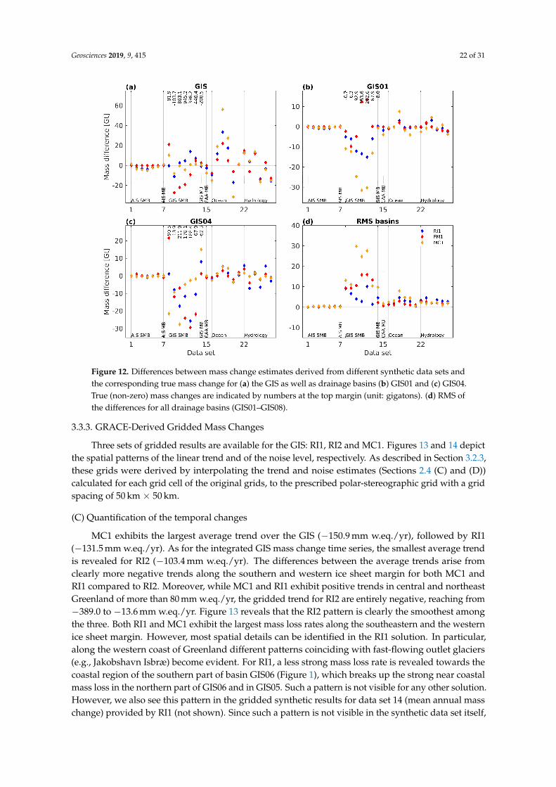


![Short-term transport variability of the Antarctic ...klinck/Reprints/PDF/bergmannJGR2012.pdffield, the Gravity Recovery and Climate Experiment (GRACE) [Tapley et al., 2004] satellite](https://static.documents.pub/doc/80x56/5f7ff956f454cd24954c8846/short-term-transport-variability-of-the-antarctic-klinckreprintspdf-field.jpg)


