Page 1
Graduate Theses, Dissertations, and Problem Reports
2019
Evaluating the Approach of Using NOx Control Performance Evaluating the Approach of Using NOx Control Performance
Tracking for On-Board Diagnostics of Heavy-Duty Diesel Vehicles Tracking for On-Board Diagnostics of Heavy-Duty Diesel Vehicles
Renata Castiglioni West Virginia University, [email protected]
Follow this and additional works at: https://researchrepository.wvu.edu/etd
Part of the Other Mechanical Engineering Commons
Recommended Citation Recommended Citation Castiglioni, Renata, "Evaluating the Approach of Using NOx Control Performance Tracking for On-Board Diagnostics of Heavy-Duty Diesel Vehicles" (2019). Graduate Theses, Dissertations, and Problem Reports. 3777. https://researchrepository.wvu.edu/etd/3777
This Thesis is protected by copyright and/or related rights. It has been brought to you by the The Research Repository @ WVU with permission from the rights-holder(s). You are free to use this Thesis in any way that is permitted by the copyright and related rights legislation that applies to your use. For other uses you must obtain permission from the rights-holder(s) directly, unless additional rights are indicated by a Creative Commons license in the record and/ or on the work itself. This Thesis has been accepted for inclusion in WVU Graduate Theses, Dissertations, and Problem Reports collection by an authorized administrator of The Research Repository @ WVU. For more information, please contact [email protected] .
Page 2
Evaluating the Approach of Using NOx Control Performance Tracking for On-Board
Diagnostics of Heavy-Duty Diesel Vehicles
Renata Castiglioni
Thesis submitted
to the Benjamin M. Statler College of
Engineering and Mineral Resources
at West Virginia University
in partial fulfillment of the requirements for the degree of
Master of Science in
Mechanical Engineering
Arvind Thiruvengadam, Ph.D., Chair
Marc Besch, Ph.D.
V’yacheslav Akkerman, Ph.D.
Department of Mechanical and Aerospace Engineering
West Virginia University
Morgantown, West Virginia
2019
Keywords: Diesel Exhaust Emissions, Nitrogen Oxides, Onboard Diagnostic, Onroad
Testing
Copyright 2019 Renata Castiglioni
Page 3
ABSTRACT
Evaluating the Approach of Using NOx Control Performance Tracking for
On-Board Diagnostics of Heavy-Duty Diesel Vehicles
Renata Castiglioni
Regulatory agencies have taken several measures to ensure proper regulation of engine exhaust
in response to a yearly rise in urban pollution levels. This is due in no small part to vehicular traffic
and resulting air pollution from exhaust.
This study evaluates the NOx Control Performance Tracking (NCPT) Onboard Diagnostic
(OBD) parameter proposed by the California Air Resources Board (CARB) as a tool to assess in-
use heavy-duty vehicle performance. It also assesses the various criteria prescribed in the NCPT
approach for applicability to real-world vehicle data.
In order to analyze the data, the study also investigated the effect of various filter constants
values over the cumulative values binned into the various categories. The study also illustrates the
differences in the bin statistics as a function of vehicle activity and it evaluates the applicability of
the NCPT approach for evaluating Not-to-Exceed (NTE) operation. The collected data displayed
abnormalities which could be attributed to sensor limitations. This project proposes two options to
reduce the noise in the sensor’s data. In the first, it uses the NOx stable channel – if available –
and the second is the exponentially weighted moving average (EWMA). Both reducing methods
were then compared to the original raw dataset to ensure no over smoothing of the data occurred.
Once these datasets were finalized, they went through the Moving-Average Window (MAW)
method proposed by EURO VI regulations before they could be binned.
The results indicate that despite applying different methods for NOx data reduction, the final
binning product only displayed small change in value for certain bins while some remained intact.
In addition, the vehicle displayed very few values inside the NTE zone, accounting at the most for
17% of the engine’s operation.
Page 4
iii
Acknowledgements
First and foremost, I would like to thank my Committee Chairperson Dr. Arvind
Thiruvengadam for providing me with the opportunity to perform research in the field of my
interest in addition to his teaching and guidance throughout the program. Your mentorship and
patience were fundamental to my completion of this program. Additionally, I would like to thank
my other committee members, Dr. Marc Besch and Dr. V’yacheslav Akkerman, for their time and
consideration of my thesis.
I would also like to thank my friends and coworkers for their support and friendship. To
Rasik, I genuinely appreciate all you’ve done for me. Without your mentorship and instructions, I
would have struggled greatly through the program; you really were a mentor to me. I would also
like to thank Sarah for always supporting me, and her companionship when I needed to spend time
with a friend. Thanks are also due to Chakri and Sam for being outstanding office-mates; you were
there when I needed a break from work and always provided me with the support to spur ideas
when I thought I was at a dead end.
Additionally, I owe a debt of gratitude to my Morgantown family, the Martins, and
especially Kimberly. You took me in and made me a part of your family and supported me through
the rough times. I am very fortunate to have met you all and I can’t thank you enough for the help
and support you’ve provided.
Finally, I must thank my husband Caleb for his unfailing support despite the long days and
hours of this program. You are my best friend and my favorite person. Lastly, I’d like to thank
my puppies Luci and Bell, without whom this project would have been completed much sooner.
Page 5
iv
Table of Contents
Acknowledgements .................................................................................................................. iii
List of Figures .......................................................................................................................... vi
List of Tables ......................................................................................................................... viii
1. Introduction ...................................................................................................................... 1
Objective ................................................................................................................... 2
2. Literature Review ............................................................................................................. 3
History....................................................................................................................... 3
Background ............................................................................................................... 4
NOx Formation .................................................................................................. 4
NOx Regulation ................................................................................................. 6
Measurement Techniques ................................................................................ 11
Regulatory .................................................................................................... 11
Onboard Zirconia Sensor ............................................................................. 15
Onboard Diagnostic (OBD) System ................................................................ 17
Moving-Average Windows (MAW) ............................................................... 17
3. Methodology .................................................................................................................. 19
Vehicle Selection .................................................................................................... 19
Data Setup ............................................................................................................... 19
Filtering Raw NOx Data .................................................................................. 19
NOx Stable ................................................................................................... 20
Exponentially Weighted Moving Average (EWMA) .................................. 20
NOx Conversion .............................................................................................. 21
Torque, Work, and Power ................................................................................ 22
NTE Method ........................................................................................................... 22
Binning .................................................................................................................... 23
4. Results and Discussion ................................................................................................... 26
Lug Curve and NTE Zone ....................................................................................... 26
NOx Data Reduction ............................................................................................... 27
NOx Stable Method ......................................................................................... 27
EWMA Method ............................................................................................... 28
Binned Data ............................................................................................................ 31
Monthly ........................................................................................................... 31
NOx Stable ................................................................................................... 37
Page 6
v
EWMA ......................................................................................................... 38
Weekly ............................................................................................................. 39
NOx Stable ................................................................................................... 42
EWMA ........................................................................................................ 43
Daily ................................................................................................................ 44
NOx Stable ................................................................................................... 46
EWMA ........................................................................................................ 47
Limitations .............................................................................................................. 48
5. Conclusions and Recommendations............................................................................... 49
Conclusion .............................................................................................................. 49
Recommendations ................................................................................................... 50
6. References ...................................................................................................................... 52
Appendix A: Bin Plots for Week Dataset ............................................................................... 56
Appendix B: Bin Plots for Daily Dataset ................................................................................ 59
Page 7
vi
List of Figures
Figure 1 - NOx Emissions Standards for Heavy-Duty Diesel Vehicles Timeline [44] ............ 7
Figure 2 - NTE Zone Representation for a Generic Engine Torque Curve [18] .................... 10
Figure 3 - Chemiluminescent Detector Working Principle [20] ............................................. 12
Figure 4- Electrochemical Sensor Representation [46] .......................................................... 13
Figure 5 - PEMS Flow Diagram [25] ..................................................................................... 14
Figure 6 - Zirconia Based NOx Sensor Representation [3] .................................................... 15
Figure 7 - FTIR vs PEMS vs NOx Sensor [28] ...................................................................... 16
Figure 8 - NOx Tracking Binning Proposal [45] .................................................................... 24
Figure 9 - Lug Curve and NTE Zone for the Desired Vehicle ............................................... 26
Figure 10 - NOx data filtered with NOx Stable vs Original Data .......................................... 28
Figure 11 – Amplified NOx data filtered with NOx Stable vs Original Data ........................ 28
Figure 12 - Filtered NOx EWF=0.1 vs Original data ............................................................. 29
Figure 13 - Amplified Filtered NOx EWF=0.1 vs Original data ............................................ 29
Figure 14 - Filtered NOx Data vs Original ............................................................................. 30
Figure 15 - Amplified Point 1: Filtered NOx Data vs Original .............................................. 30
Figure 16 - Amplified Point 2: Filtered NOx Data Peaks vs Original Data ........................... 31
Figure 17 - Original Data NOx (g/bhp-hr) Bin - Monthly ...................................................... 32
Figure 18 - Original Data NTE Bin - Monthly ....................................................................... 33
Figure 19 - Original Data Bin Count - Monthly ..................................................................... 33
Figure 20 - Original Data Post-SCR Exhaust Temperature (oC) Bin - Monthly .................... 34
Figure 21 - Original Data Power (bhp) Bin - Monthly ........................................................... 35
Figure 22 - Original Data NOx (g) Bin - Monthly .................................................................. 35
Figure 23 - Original Data Distance (miles) Bin - Monthly ..................................................... 36
Figure 24 - Stable Reduction Method NOx Data (g/bhp-hr) Bin - Monthly .......................... 37
Figure 25 - EWMA Method (EWF=0.1) NOx Data (g/bhp-hr) Bin - Monthly ...................... 38
Figure 26 - EWMA Method (EWF=0.25) NOx Data (g/bhp-hr) Bin - Monthly .................... 38
Figure 27 - EWMA Method (EWF=0.35) NOx Data (g/bhp-hr) Bin - Monthly .................... 39
Figure 28 - Original Data NOx (g/bhp-hr) Bin - Weekly ....................................................... 40
Figure 29 - Original Data NTE Bin - Weekly ......................................................................... 40
Figure 30 - Stable Reduction Method NOx Data (g/bhp-hr) Bin - Weekly ............................ 42
Page 8
vii
Figure 31 - EWMA Method (EWF=0.1) NOx Data (g/bhp-hr) Bin - Weekly ....................... 43
Figure 32 - EWMA Method (EWF=0.25) NOx Data (g/bhp-hr) Bin - Weekly ..................... 43
Figure 33 - EWMA Method (EWF=0.35) NOx Data (g/bhp-hr) Bin - Weekly ..................... 44
Figure 34 - Original Data NOx (g/bhp-hr) Bin - Daily ........................................................... 45
Figure 35 - Original Data NTE Bin - Daily ............................................................................ 45
Figure 36 - Stable Reduction Method NOx Data (g/bhp-hr) Bin - Daily ............................... 46
Figure 37 - EWMA Method (EWF=0.1) NOx Data (g/bhp-hr) Bin - Daily........................... 47
Figure 38 - EWMA Method (EWF=0.25) NOx Data (g/bhp-hr) Bin - Daily......................... 47
Figure 39 - EWMA Method (EWF=0.35) NOx Data (g/bhp-hr) Bin - Daily......................... 48
Figure 40 - Original Data Post-SCR Exhaust Temperature (oC) Bin - Weekly ...................... 56
Figure 41 - Original Data Power (bhp) Bin - Weekly ............................................................ 56
Figure 42 - Original Data Distance (miles) Bin - Weekly ...................................................... 57
Figure 43 - Original Data NOx (g) Bin - Weekly ................................................................... 57
Figure 44 - Original Data Bin Count - Weekly ....................................................................... 58
Figure 45 - Original Data Post-SCR Exhaust Temperature (oC) Bin - Daily ......................... 59
Figure 46 - Original Data Power (bhp) Bin - Daily ................................................................ 59
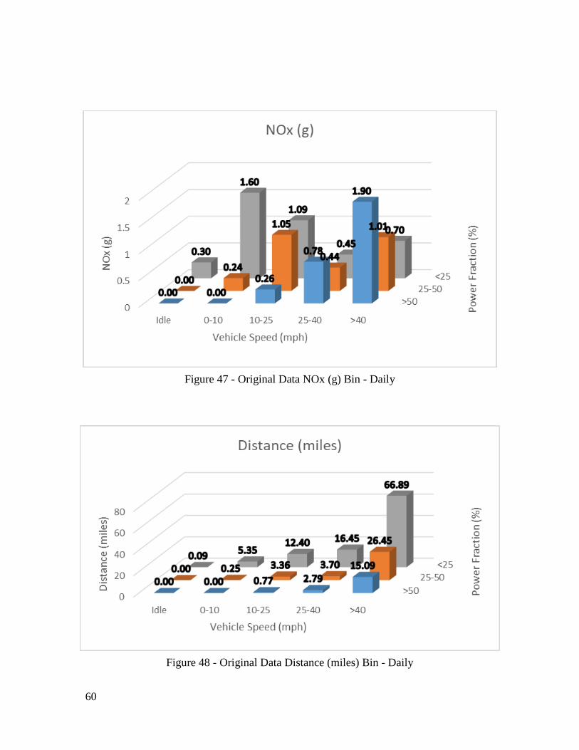
Figure 47 - Original Data NOx (g) Bin - Daily ...................................................................... 60
Figure 48 - Original Data Distance (miles) Bin - Daily .......................................................... 60
Figure 49 - Original Data Bin Count - Daily .......................................................................... 60
Page 9
viii
List of Tables
Table 1 - Nitrous Oxides Types and Properties [12] ................................................................ 5
Table 2 - Heavy-Duty Highway Diesel Engines EPA Emissions Standards [47] .................... 9
Table 3 - Proposed Bin Structure According to CARB as of 2018 ........................................ 25
Table 4 - WBW and Binning Analysis Method ...................................................................... 25
Table 5 - Boundary Conditions for NTE Zone ....................................................................... 27
Table 6 - Total Duration Summary - Monthly ........................................................................ 32
Table 7 – Total Duration Summary - Weekly ........................................................................ 41
Table 8 - Total Duration Summary - Daily ............................................................................. 44
Page 10
1
1. Introduction
Air pollution as a result of vehicle exhaust, has been a concern to human health world over for
decades. It’s well established that heavy-duty diesel (HDD) engines produce more oxides of
nitrogen (NOx) than similar gasoline engines [1]. Several studies have been conducted to reduce
emissions by studying the effects of different after treatment systems when added to the exhaust
system. Despite continuous progress in emission technologies, overall emissions still continue to
rise due to an increase in both number of vehicles and average yearly mileage traveled by vehicles
within the United States [2]. In response, the United States government has committed to
regulating emissions in conjunction with the engine manufacturers in order to minimize the
emission profiles of these engines. However, as exhaust aftertreatment systems (EATS) become
more complex there has been a growing need to determine appropriate means to ensure the proper
working of the complex EATS. The current federal test procedure (FTP) cycle is not the most
accurate representation of real-world vehicle activity [3]. There exists significant difference in
real-world emissions rates and certification data [4]. In response, the California Air Resources
Board (CARB) is in the process of introducing the window-averaging method to bin NOx data for
standard evaluations of emission data regardless of route or driving cycle. This method is referred
as the NOx Control Performance Tracking (NCPT) or Real Emissions Assessment Logging
(REAL). This program has been recently implemented as part of the OBD regulations, which
emphasize the use of current technology to analyze current onroad emission [5].
As part an effort to improve analysis of vehicular emissions profile and inform meaningful
regulations, West Virginia University (WVU) was selected to conduct a study in California where
researchers collected onroad data for multiple makes and models of heavy-duty vehicles. Sensors
were attached to these vehicles before returning the vehicles to their usual schedule. Data was
recorded for at least three months for each of the vehicles tested. The resulting datasets were then
evaluated to better inform understanding of the emissions profile.
Page 11
2
Objective
The goal of this study was to analyze real-world data using a binning approach to characterize
vehicle activity and in-use emissions for the purposes of OBD. The specific objective of the study
included the analysis of real-world telemetry data in accordance to a binning method proposed by
CARB. The main objective was to investigate the on-road emission data for a better understanding
of the engine operation condition beyond test cycles. To do so, data was analyzed daily, weekly,
and monthly in order to create consistent frames of reference when analyzing data sets.
Page 12
3
2. Literature Review
History
The first petroleum-based automobile was invented in Germany in the late 1800s. By the end
of the first half of the twentieth century, the United States had become a major manufacturer of
automobiles due to the perfection of mass production techniques first developed by Henry Ford.
With the exception of a short stall in vehicle sales in 1927, the automotive industry has continued
to grow yearly and accounts for vehicles from vocational cars to heavy duty vehicles [6].
The increase in vehicles sales and supporting infrastructure via highway building projects has
also led to an increase in air pollution across the United States. This problem is specifically
pronounced in cities due to the high volumes of vehicle traffic confined to a smaller area. In 1943,
Los Angeles reported the first ever smog cloud which resulted in multiple health problems for
residents. This first ever smog cloud incident was so pronounced that some residents were led to
believe it was the result of a Japanese chemical weapons attack. It wasn’t until 1948 that scientists
discovered that smog was the result of vehicle exhaust and industrial pollution [7]. By 1955, in
response to a growing concern for the health hazard caused by air pollution, the Department of
Health, Education, and Welfare authorized the first air pollution program. This was the first
instance of government’s attempt to legislate air pollution and conduct research on the sources of
pollution through the Air Pollution Control Act [8]. As an improvement to prior legislation, the
Clean Air Act (CAA) of 1963 was passed. The CAA was intended to reduce pollution by holding
each state responsible for its own control activities. In turn, the Department of Health, Education,
and Welfare would conduct research into air pollution using federal funds. In 1965, the CAA was
improved when amendments were passed to create national standards for motor vehicle pollution.
However, it wasn’t until 1967 when President Johnson asked Congress to pass new legislation that
would enhance research and control efforts. As a result, Congress passed the Air Quality Act near
the end of 1967. This new legislation aimed to expand funds for pollution research, air quality
monitoring, and emissions control strategies [9].
By 1970, amendments were made to the 1963 CAA despite a decrease in air pollution across
the United States. The 1970 amendments allowed both state and federal government to regulate
emissions at both the industrial and individual level. It also established the National Emission
Standards for Hazardous Air Pollutants (NESHAP), the National Ambient Air Quality Standards
Page 13
4
(NAAQS), and required individual states to plan for a means of meeting these standards. It was
during this same period that the Environmental Protection Agency (EPA) was established to
implement the requirements of this new legislation. The EPA is still a major government agency
responsible for pollution regulation in the United States. In 1977 and 1990, additional amendments
were passed to the 1963 CAA to increase the authority of the federal government to regulate
pollution and maintain air quality standards [8]. Throughout the years the regulations have gone
from nonexistent in early 1950s to extremely strict. For instance, currently the NOx standard for
HDD vehicles is 0.2 g/bhp-hr and California even offers an optional low NOx standard of 0.02
g/bhp-hr [10].
Background
NOx Formation
In compression ignition (CI) engines – Diesel engines – fuel and air are not mixed until both
are injected into the cylinder and the ignition process starts. In CI engines, combustion follows the
diffusion combustion pattern, whereby the fuel and oxidizer mix during the combustion process.
When comparing engines, engines utilizing the CI combustion process produce a higher
compression ratio and therefore increased efficiency in relation to spark ignition (gasoline)
engines. However, this increased efficiency comes at the cost of higher particulate matter and NOx
emissions [11].
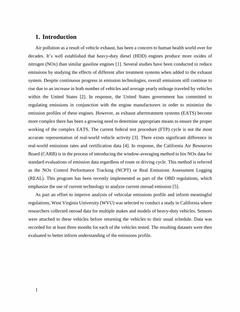
Nitrogen oxides (NOx) is a family composed of multiple compounds. Table 1 displays the list
of compounds within the NOx family. However, the EPA only regulates nitrogen oxide (NO) and
nitrogen dioxide (NO2), which are the most common NOx compounds present in engine exhaust
gas. Therefore, for the purpose of this project, NO and NO2 are the only NOx family compounds
referenced when the author uses the term NOx [12].
Page 14
5
Table 1 - Nitrous Oxides Types and Properties [12]
NO is a common compound formed in the atmosphere; however, a percentage of NO present
is the result of fuel combustion. The governing equations that summarize the formation of NO can
be described in the following manner, which is often referred to as the Zeldovich mechanism [1].
O+N2→NO+N (1)
N+O2→NO+O (2)
N+OH→NO+H (3)
The formation of NO can occur at both the flame front as well as the end of combustion gases.
In fact, during normal engine function the majority of NO is formed at the end of the combustion
cycle. The formation of NO is mostly dependent on temperature. Higher temperatures combined
with high oxygen concentrations will result in the formation of more NO relative to lower
temperatures. Additionally, at the flame zone, NO can convert into NO2 and NO2 can convert into
NO by the following processes described by equations (4 and (5. The latter process won’t occur if
the flame is mixed with a cooler fluid meaning that the highest NO2 to NO conversion occurs at
light loads when the cylinders still contain cooler sections that could quench the flame [1]. The
primary emitter from the engines is known to be NO [12].
Page 15
6
NO+HO2→NO2+OH (4)
NO2+O→NO+O2 (5)
NOx compounds may form nitric acid (HNO3) or nitrous acid (HNO2) when dissolved in water.
Both compounds are well known to influence the rate of acid rain events. The NOx compounds
are known to be naturally produced in nature and are commonly found in the air. Therefore, any
addition of NOx from outside sources can result in an oversaturation of these compounds in the
air. However, NO is mostly produced by human activities. The natural sources are assumed to
account for less than 10% of its emissions. Both NO and carbon dioxide (CO2) are known to cause
difficulties for the blood to absorb oxygen, which is a threat to human health. As for NO2 the main
concern is its tendency to produce ozone (O3) which in excess is the main contributor for smog
[12].
NOx can also have profound impacts on aquatic life. A process called eutrophication can occur
when there’s an excess of nitrates present in water. Eutrophication is the process by which
phytoplankton produce a surplus of nutrients which in turn cause excessive growth of certain plants
in freshwater and saltwater environments that deplete the area of oxygen resulting in the death of
marine life and aquatic plants [12]. This highlights the multiple factors driving regulations for a
reduction of these gases.
NOx Regulation
According to the EPA, in 1997 the ozone pollution became an urgent matter regarding health
hazards affecting millions of Americans. The areas designated as non-attainment were facing
issues reaching the desired air quality and/or maintaining the quality. As a result, there was a need
to regulate the emissions of NOx, hydrocarbons, and particulate matter for heave-duty engines. It
was in 1997 that the EPA in association with the manufactures came together to create control
strategies for NOx for onroad HDD vehicles [13]. This was the first attempt to reduce NOx
emissions focused solely on HDD vehicles. Since 1997 multiple other regulations were passed in
order to further decrease NOx emissions. As part of a study Figure 1 shows how the regulations
have evolved from 1985 to the 2010 NOx regulation proposed by the CARB.
According the U.S. EPA NOx main sources are automotive, power plants, and off-road
equipment. This main method that this family of compounds gets in the air is from the burn of
Page 16
7
fossil fuel [14]. In addition, NOx can also react with ozone and form acid rain [12]. As a result,
there’s a continued effort from multiple agencies to regulate and decrease the amount of NOx
emitted every year. The number one NOx emitter in the United States is the agriculture sector.
However, agriculture is difficult to regulate due to NOx emissions resulting mainly from fertilizers
and soil treatments which are necessary to maintaining growth rate of crops. Fuel combustion only
accounts for about 5% of the total NOx emission, however it has displayed a 4% increase since
1990 making it an easier target for reduction by regulation [13].
Diesel engines tend to produce more NOx than gasoline engines due to the method of fuel
mixture. While gas engines rely on a premixed combustion method, diesel engines have a diffusion
combustion method. Due to the diffusion combustion method, the fuel and air are mixed inside of
the combustion chamber turning it into a heterogeneous mixture. The resulting variables of
combination of the heterogeneous mixture, ignition delay, and fuel to air ratio influence the amount
of NOx generated during combustion [15]. There have been multiple studies conducted in addition
Figure 1 - NOx Emissions Standards for Heavy-Duty Diesel Vehicles Timeline [44]
Page 17
8
to current studies in development to maximize the combustion efficiency of diesel engines and
decrease NOx formation. However, due to the nature of combustion it’s impractical to assume that
NOx formation can be completely eliminated during the diffusion combustion process. To mitigate
the NOx formation, aftertreatment systems have been developed to assist the reduction of the
emissions.
For diesel engine emissions the main concern is NOx, therefore the vehicles are usually
equipped with selective catalytic reduction (SCR) technology to reduce NOx. A SCR that is
working properly can reduce NOx emissions by almost 90% [16]. Additional aftertreatment
systems common in diesel engine vehicles include diesel exhaust fluid (DEF) which is added to
the exhaust before it goes through the SCR, a diesel particulate filter (DPF), and a diesel oxidation
catalyst (DOC). For the SCR to function as intended, first the DEF must be injected into the
exhaust flow – which is usually composed of urea – and through a reduction reaction NOx breaks
down into nitrogen gas and water [17]. However, the SCR system function is dependent on
temperature. The chemical reaction doesn’t start until the system temperature reaches at least
2000C. If the SCR system is operating below 2000C the SCR is highly inefficient. Temperature
dependency causes fluctuation in diesel engine emissions due to the tendency of diesel engines
operating at low speeds under low loads to not reach desired temperature resulting in higher than
normal NOx emission. Therefore, even with multiple aftertreatment systems already in place, the
United States EPA frequently passes regulations to incentivize the development of technologies to
negate the need for a temperature dependent system. For instance, in Figure 1 the US EPA set a
NOx limit of 0.2 g/bhp-hr in 2010 and as of 2013 the CARB has stablished a new optional ultra-
low NOx standard of 0.02 g/bhp-hr. However, there are still multiple studies being conducted in
order to analyze the feasibility of this new ultra-low standard [10]. The table below summarizes
the standards over the years for heavy-duty compression-ignition engines as of 2016.
Page 18
9
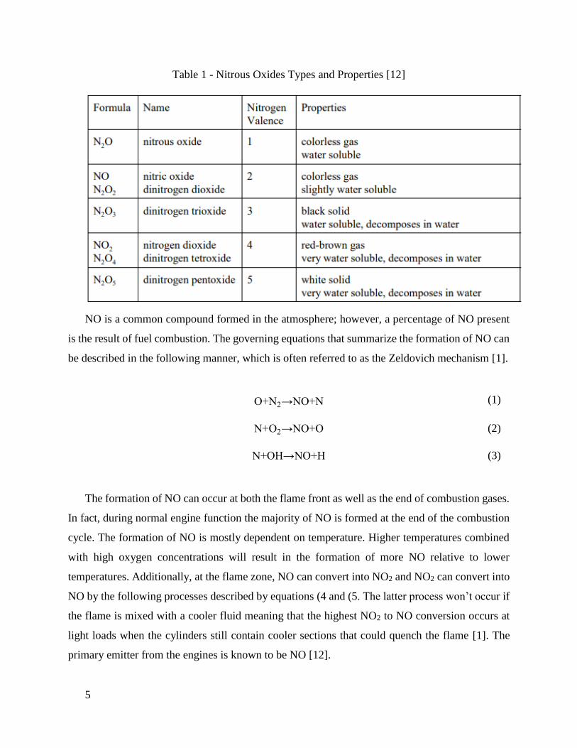
In addition to the regulations described above, the EPA has also implemented the Not-To-
Exceed (NTE) mission limit to analyze the HDD engine’s emissions over a defined operation
region under a set of rules that qualify to be an NTE operation. In theory, NTE operation method
is to represent real-world long-haul truck operation [18].
Not-To-Exceed (NTE):
This approach takes in consideration that every engine has a control area, in which its emission
values must be compliant. This region contains the values which represent the engine’s expected
engine speed and load under normal operation. In Figure 2, the blue area represents the NTE zone
for the particular engine used for that map, which is bounded by the torque curve and the 30%
peak torque, and the speed threshold (n15). For the emissions to be within this category they must
be quantified over a period of 30 seconds before being compared to the NTE emissions standard
[4].
In addition to the boundary conditions provided in Figure 2, the NTE cycle also has a
temperature conditions that must be met. For the temperature to be considered compliant (TNTE) it
Table 2 - Heavy-Duty Highway Diesel Engines EPA Emissions Standards [47]
Page 19
10
must lower than the ambient temperature which is also dependent on altitude [4]. The equations
bellow (6-8) displays the relationship between those variables.
AltitudeNTE≤5,500 ft (6)
TNTE<TAmbient (7)
TAmbient=-0.00254×Altitude(ft)+100 (8)
For engines that are equipped with an exhaust gas recirculation (EGR) system there are two
more exclusions that should be included. These conditions remove NTE points if it’s under cold
temperature conditions. It requires that the intake manifold temperature (IMTEGR) to above or
equal to the NTE reference IMT, and that the engine coolant temperature to be larger than the NTE
reference value (ECTEGR) [18].
IMTEGR(℃)=11.428×IMPabs(bar)+88.571 (9)
ECTEGR(℃)=12.853×IMPabs(bar)+127.11 (10)
This approach however does have several limitations. For instance, the strict boundaries of the
NTE zone as well as the minimum event duration limits the amount of data inside the control zone.
Figure 2 - NTE Zone Representation for a Generic Engine Torque Curve [18]
Page 20
11
Depending of the vehicle’s type of operation the driver may perform frequent gears change or have
stop and go driving cycle. These driving operations may possibly exclude the data from the NTE
zone. This indicates that this method may not be applicable to all vocations. In addition, the need
for ambient condition and additional engine data results in a need for several more channels in the
ECU which may not all be present for the required period (30 seconds) [4]. A more detailed
explanation of the calculations used for this method can be found in the methodology section.
Measurement Techniques
Regulatory
Besides the commonly used zirconia sensor, there are several technologies that have been
developed to detect NOx in diesel engine exhaust. Some of these technologies are more accurate
than the smaller zirconia sensor, however they all have unique drawbacks. The following are some
of the NOx sensor data acquisition methods and technologies acknowledged by EPA.
NOx Chemiluminescent Detector (CLD):
The NOx CLD system can only detect NO, therefore requiring a catalyst to first convert NO2
to NO prior to detection. When NO and O3 react, they produce NO2+ (excited state), this reaction
produces photons [19]. This light (photons) can be counted with a photon counter that uses a photo
multiplier tube to detect the photons. The output voltage from this process can then be linearly
correlated to the NO concentration [20]. Figure 3 is a representation of the device and how it works.
The NOx CLD system requires zero air supply but is quite large and expensive, making it a less
than desirable candidate for onroad emissions data collection [21].
Page 21
12
Electrochemical NO Sensor:
Electrochemical NO sensors contain cells that only sense NO, which one more requires a
catalyst for the conversion. This cell is known to be very small and relatively inexpensive
compared to the other analyzers. However, this sensor is known to have a slower response time
which impairs accuracy. Additionally, a high relative humidity can also affect the sensor’s
performance which requires corrections for accurate function [21].
The electrochemical NO sensor is usually amperometric and it operates by producing an
electrical signal when it reacts with the analyte. The desired compound goes through either
oxidation or reduction in an electrode and the concentration can be estimated from the output
current [22]. Figure 4 displays a simple representation of this sensor, where the sensor in this figure
is detecting carbon monoxide instead of NOx.
Figure 3 - Chemiluminescent Detector Working Principle [20]
Page 22
13
Nondispersive Infra-Red (NDIR) NO Analyzer with Luft Detector:
Similarly to the other analyzers the NDIR NO analyzer with Luft Detector can only detect NO,
therefore it requires a catalyst to first convert NO2 to NO. The NDIR system is usually used for
CO/CO2 data collection, however with the addition of the Luft detector it can be used for NO
detection. A Luft detector uses a non-dispersive optical analyzer to select the gas to analyze, which
makes it more sensitive to wavelengths of the desired chemical instead of the other compounds in
the exhaust gas. The system consists of a diaphragm between two sealed cells that contains the
desired gas that will be analyzed. In the diaphragm a deflection occurs when there’s a difference
in pressure between the cells. By measuring the deflection with a capacitor, the NDIR NO analyzer
can estimate the concentration of the desired gas. Because this system requires the Luft detector it
is quite sensitive to vibrations which makes it unsuitable to onroad operations [21].
Nondispersive Ultraviolet Detector (NDUV):
The NDUV detector is a commonly used device to measure NOx [23]. This analyzer guides
the sample gas through a chamber where it measures the wavelength of the gas when it absorbs
light. These wavelengths allow the detector to return information regarding the gas composition.
This system even though has good performance and accuracy, it is relatively large and complex
for onroad applications [24].
Figure 4- Electrochemical Sensor Representation [46]
Page 23
14
Portable Emissions Measurement System (PEMS):
The PEMS system, which uses either a chemiluminescent or NDUV detector, has the most
reliable real-time measurement when compared to all the previously described systems. It provides
continuous and accurate measurement of multiple gases (NOx, CO, CO2, and THC). The system
is also capable of measuring accurate exhaust flow rate from the Engine Electronic Control Module
(ECM) or the exhaust flow meter and GPS data [25]. The following figure represents the PEMS
flow diagram according the CARB.
A PEMS can measure concentration for each gas utilizing different methods. For instance, a
PEMS unit can be equipped with a chemiluminescent section so it can measure NOx while using
a NDIR for the other compounds. This ability to use multiple methods in one unit to measure the
exhaust flow makes the unit extremely versatile and valuable for research. However, it may be
impractical for onroad applications because unit is too large and expensive to be added to every
vehicle [26].
Figure 5 - PEMS Flow Diagram [25]
Page 24
15
Onboard Zirconia Sensor
The yttrium-stabilized ZrO2 (YSZ) is most commonly used for NOx emission onroad data due
to its size and cost effectiveness in comparison to the PEMS system. This type of sensor contains
two chambers usually coated with platinum [3]. The first cell removes O2 so it won’t interfere with
the sample while the other cell dissociates NO into N2 and O2. The O2 removed from the second
cell allows the sensor to calculate the NOx concentration by determining the voltage required to
remove the O2 caused by the dissociation [21]. For optimal results, the NO2 should be first
converted into NO using a catalyst, such as the SCR [27]. Figure 6 displays YSZ sensor operation.
The data is then broadcasted publicly through the J1939 CAN communication protocol.
In 2002 WVU conducted a study where it compared the ZrO2 sensor to well established
analyzers, such as the NDIR. Despite indications that the zirconia sensor displays errors between
6-12% for lower NOx concentrations in the 5-175 ppm range, the study concluded that the ZrO2
sensor was found to be the best device for onboard measurements when comparing accuracy and
Figure 6 - Zirconia Based NOx Sensor Representation [3]
Page 25
16
cost effectiveness [21]. Later in the study performed by Thiruvengadam et al. [28] the data from
OBD-NOx was compared to the data from the control volume system (CVS) as well as PEMS in
order to analyze the limitations of these sensors. At high concentrations the OBD sensor displayed
readings within 10% of the PEMS and CVS, while at lower concentrations were the SCR
functioned properly the values between the OBD sensor and the other two systems had a much
larger difference. Overall, the sensor displayed acceptable results when compared to PEMS and
FTIR measurements. However, the authors suggest that for a more accurate dataset a predictive
algorithm or filtering algorithm could be used in the sensor data. The authors note that the large
errors could be attributed to the original equipment manufacturers’ (OEM) method to
correct/predict the data. Figure 7 displays the results from the study.
Some of the limitations of this sensor includes being affected by multiple engine subsystems
such as the SCR catalyst deterioration, urea dosing control and EGR control. In addition, the sensor
may be turned off during the vehicle operation for the safety of the device [29]. Also, the sensor
can’t differentiate the components of the exhaust gas. Therefore, it has a high cross-sensitivity
with certain compounds such as ammonia, isocyanic acid (HNCO), and hydrogen cyanide (HCN).
HCN is usually found in ethanol systems. Most of these compounds are a result from the urea
dosing control system defects [30]. Note that this sensor required a temperature of 700 oC to work
Figure 7 - FTIR vs PEMS vs NOx Sensor [28]
Page 26
17
properly, therefore during cold start operation the sensor doesn’t record reliable data [3]. Because
of the high temperature water droplets may affect the sensor by causing rapid cooling [21].
Onboard Diagnostic (OBD) System
Over the years CARB and the EPA have implemented several regulations for the types of
technologies and systems used in the acquisition and monitoring of data, and emissions standards
for the vehicles, some of the regulations cover onboard diagnostic (OBD) systems. The system can
be referred as either OBD or OBD II, where the later describes the last generation of the technology
[31]. These regulations can be found in the California Code of Regulations (CCR) or in the Code
of Federal Regulations (CFR). While most states only must comply with the CFR the vehicles used
in California must be in compliance with both regulations. The OBD has the purpose of monitoring
the engine’s emissions and detecting any possible malfunction in the emissions system based on
the current emissions standards. While the Clean Air Act Amendments (CAAA) only required the
monitoring of the catalyst and oxygen sensor, the OBD regulation now requires the monitoring of
several system for emission control such as the EGR, misfire, oxygen sensor heater, and others
[32]. These malfunctions should be displayed to the vehicle operator and also recorded in the
onboard computer system [31].
According to the CFR, all vehicles MY 2017 or later must be equipped with an OBD system
and the system must comply with CCR’s OBD II requirements. Note that all light-duty trucks and
complete heavy-duty vehicles weighing 14,000 pounds of gross vehicle weight rating (GVWR) or
less must have OBD system [33]. The system must be able to monitor the engine system and
emissions throughout the useful life [32]. The regulation is reviewed and regulated every year.
According to title 13 section 1971 of the CCR [32], the OBD system should be able to operate
without any type of maintenance. The system is also not allowed to be programed.
Moving-Average Windows (MAW)
There are multiple studies that have aimed to understand and better analyze the emission data
recorded by the onboard sensors. For instance, in 2008 WVU Center of Alternative Fuels Engines
and Emissions (CAFEE) proposed the use of WBW method to calculate break-specific NOx
(bsNOx) for HDD engine. Shade et al. [34] describes that as long as the Engine Control Unit
Page 27
18
(ECU) broadcasts all channels that are needed to calculate NOx and work – which are later
described in detail – this method can be easily used. In order to perform this method, first the
instantaneous work (bhp-hr) and NOx rate (g/s) must be calculated using the ECU channels. The
following equations describes how the bsNOx can be calculated, where N is the engine speed, T
is engine Torque, and t is time, and Δt is the window duration in seconds.
WorkWindow(bhp-hr)=∑
(
Ni (
revmin
)×Ti(ft-lb)
(1 rev2π rad
) (60 sec1 min
) (550ft-lbf
1 sec-bhp)
×∆ti(sec)× (1 hr
3600 sec)
)
i*
i=0
(11)
bsNOx (g
bhp-hr)=∑ NOxi (
gsec) *∆ti(sec)i
*
i=0
WorkWindow(bhp-hr)
(12)
The WBW method has some limitations, such as the data becomes invalid if the pressure is
less than 82.5 kPa, the ambient temperature is less than -7 oC, engine coolant temperature is less
than 70oC, and altitudes above 1600 m [3]. This method follows a similar approach to the MAW.
In order to bin the data, first it must go through MAW. This method is acknowledged by the
Euro VI Regulation [35]. The moving average can function as a way to smooth the data by
replacing a segment of data points with their average. These averages are stored into windows
which are later compiled into one vector [36]. Like the WBW, this method could be used to analyze
the exhaust temperature, distance, and power. Where for each of these parameters the dataset is
compiled in segments (windows) for a specific amount of time, also known as the data sampling
period (Δt). According to CARB the sampling period should be set for 15 seconds [37]. The
following equations were used to generate the window for the other parameters. Similar to equation
(13, where ‘i’ indicates the window number (individual variables, e.g. Window1, Window2, etc.).
The final continuous vector can be created by concatenating the windows as shown in equation
(14, Wparameter is the new vector for a specific parameter after it goes through the averaging window
method and count is just a variable used to keep track of the windows created by the this procedure
(e.g. Wparameter(1,1), Wparameter(2,1), Wparameter(3,1), etc.).
Window(i,1)=mean(Parameter(t:t+∆t-1)) (13)
WParameter(count,1)=Window('count') (14)
Page 28
19
3. Methodology
Vehicle Selection
In order to properly analyze the data, first the manufacturers must provide enough parameters
that are streamed by the ECU. The availability of the channels dictates which vehicles are suitable
to be used for the analysis and which ones aren’t. Certain channels can’t be easily estimated, such
as the exhaust mass flow which requires refined algorithms to be estimated. This parameter could
alone remove a vehicle from the list of suitable vehicles. Alongside the exhaust mass flow channel,
the raw NOx channel must be present as well. The data from this channel should come from a
sensor located downstream the aftertreatment section of the exhaust pipe. There are several other
channels that are desired for this type of study; however, they are more commonly found than the
previous ones stated.
Based on the needs described above a simple program can be generated to analyze each
individual vehicle available and generate a spreadsheet for each one of them describing the quality
of each file and availability of each channel. By using MATLAB, a code was generated to analyze
each trip of each vehicle and return an excel spreadsheet with the channels’ availability and quality
to ensure that the channels weren’t filled with Not-a-Numbers (NaNs) or zeros. The program
returned either a 1 if the channel was available or a 0 if it wasn’t. Then it investigates the data to
see if it was composed of NaNs or zero. For this project the following channels were to be
analyzed: exhaust flow temperature, exhaust flow mass, engine speed, vehicle speed, NOx
downstream from SCR, NOx stable, and torque (nominal, actual, and reference). Certain vehicles
can display entire trips filled with NaNs, making them not suitable options. Finally, once the
spreadsheet is done a vehicle can be selected.
Data Setup
Filtering Raw NOx Data
In order to implement the tracking concept first one needs to analyze the quality of the NOx
data. That can be done by using the NOx stable channel or if it’s not present an exponentially
weighted moving average (EWMA).
Page 29
20
NOx Stable
As part of the vehicle’s ECU channels list is the NOx stable channel. This parameter works as
a control channel to the NOx raw channel. This channel indicates the stability of the NOx sensor
throughout the vehicle’s activity. For the vehicle chosen, the sections in which the value of the
NOx Stable channel was wither 1 or 3 the NOx raw channel displayed instability. Therefore, the
values in those parts were replaced with NaNs.
When calculating the bsNOx bin for this method, the position in which the NOx values were
replaced with NaNs were also applied to the work vector. Therefore, when the total NOx (g) for a
bin were divided by the total work (bhp-hr) in that same bin the amount of NaNs in each vector
were at the same position. This ensures that the total emission in the bin are not underestimating
the value in the bsNOx bin.
Exponentially Weighted Moving Average (EWMA)
Before one can explain what EWMA is, one needs to understand what a moving average is and
how it works. A simple moving average (SMA) calculates the average of n values where n
represents the number of values of which the average is taken [38]. Equation (15 below
demonstrates how it functions.
Simple Moving Average (SMA)=x1+x2+x3+…+xn
n (15)
As for the EWMA it has the same roots as the SMA method, however there’s a weigh assigned
to each point. Meaning, the early data points will have a smaller impact on the later data points
[39]. The equations below represent this method. The coefficient alpha, which is the exponential
weighting factor (EWF) is calculated based on the amount of points back in the data (n) that it
should influence the current point being calculated. This method allows the current data point
being analyzed to have more weight than the previous one when it goes through a moving average
[40]. This indicates that the method takes into consideration the vehicle’s operation history when
smoothing the set. The equation bellow represents the method. Where Pt is the original data value
at point t.
EWMAt=EWMAt-1+α(Pt-EWMAt-1) [40] (16)
α=2
n+1 [40] (17)
Page 30
21
There is a function already built in MATLAB that performs the EWMA. In order to use it, first
one must select which kind of moving average it wants to perform. For this project the method
selected was the “exponential weighting”. This method requires the user to input a value for the
exponential weighting factor (EWF) which can range from 0 to 1, where 0 would have no filtering
done and 1 has the most. Because this method can cause over smoothing of the data several
coefficients were tested. A more precise coefficient could be selected if data from PEMS was
available, but because this project did not have such data the filtered data was compared to the
original [29]. According to the 2017 HD OBD program update, CARB suggests using 0.1 for the
exponential weight coefficient value [37].
NOx Conversion
Next one must estimate the NOx mass per second using the tailpipe NOx sensor output and the
exhaust flow mass. The NOx channel output provides the concentration in parts-per-million (ppm)
while the exhaust follow channel is in kilogram-per-hour (kg/hr). Those two channels should be
available throughout the whole dataset in order to avoid time alignment issues. By using the ideal
gas law equation, and assuming the density of the fuel to be 1.2 kg/L, and standard temperature
(250C) and pressure (1 atm), the NOx rate (g/sec) can be calculated. The equations 18-21 bellow
were used to perform such calculation [41]. Note that this method does not take into account
humidity corrections, and it does use the molar mass of air for the exhaust gas.
Ideal Gas Law: PV=nRT (18)
Volumetric Flow Rate: V (L
s)=Exhaust Flow (
kg
hr)×
1hr
3600s×
1
ρ(
L
kg) (19)
Molar Rate: n (mol
s)=
Pressure(Pa) × V (Ls)
R (J
mol*K)×T(K)
(20)
NOx Mass Rate: NOx (g
s) =(NOx)ppm × 10
-6× (
mol
mol)×n (
mol
s)×MW (
g
mol) (21)
Page 31
22
Torque, Work, and Power
To properly segregate the data according to the CARB regulations, work and power fraction
must be present before the window averaging can take place. Both work and power are a function
of torque, therefore if one can calculate the engine torque from the channels provided then the
other parameters can be easily calculated. From the actual percent torque, nominal frictional
torque, and reference torque, the engine break torque can be calculated using equation (22.
Torque(lb-ft)=(TorqueActual-TorqueFrictional)×TorqueReference
100×0.73756 (22)
From the value calculated above one can now calculate the power, power fraction, as well as
work for the engine [1]. Note that the max power varies by engine and can be acquired from the
manufacturer.
Power(bhp)=Engine Speed(rpm)×Torque(lb-ft)
5252 (23)
Power Fraction=Power(bhp)
Max Power (bhp) (24)
Work(bhp-hr)=Power(bhp)
3600 (25)
NTE Method
In order to analyze onroad data, the NTE method can be used to evaluate emission for in-use
compliance based on the engine operation along specific bounds in the control area. Points which
fall in the control area are considered to be part of the engine’s normal operation. According to 40
CFR Part 86.1370, subpart C – Not-to-Exceed Test Procedures, the control area must be bounded
by the lug curve, the 30% max power, and engine speed limits (nhigh and nlow). One of the criteria
requires the engine speed (nNTE) to be higher than the variable n15 which can be calculated using
equation (27. Where nhigh represents the highest engine speed at 70% maximum power and nlow
represents the lowest engine speed at 50% maximum power [4].
nNTE>n15 (26)
n15=0.15(nhigh-nlow)+nlow (27)
If the engine speed is compliant with the specification above then the brake torque must be
equal or greater than 30% of the maximum engine torque. Finally, the instantaneous power must
Page 32
23
also be greater or above 30% of the engine’s maximum power. The torque curve, also known as
the lug curve, can be generated using the values recorded by the ECU for each of the positions of
the curve. The peak torque corresponds to the highest torque value in the lug curve. The rated
power at a specific engine speed is provided, therefore the torque corresponding to 30% of peak
power for a particular engine speed can be calculated using the equations bellow [4].
TorqueNTE=5252×Powermax (bhp)×0.3
Engine SpeedNTE (rpm) (28)
TorqueNTE≥0.3×Torquemax (29)
PowerNTE≥0.3×Powermax (30)
Binning
In addition to the MAW method, one must implement binning to perform the NOx tracking
approach by collecting data from a vehicle over time – after the data has gone through MAW - and
segregating each parameter in an array and finally binning each one of those parameters according
to specific boundaries.
In the 2017 CARB workshop [37] a proposal was made for a method to analyze real-world
NOx data. The workshop proposed to use 68 trucks with at least one-month worth of data with the
MY’s between 2010 and 2018. The trucks were from several different manufactures and vocations.
On all the data was collected for the trucks the NOx emission in g/bhp-hr was measured for each
vehicle. Only a few of the trucks were compliant with the current NOx regulation (0.2 g/bhp-hr).
The workshop then used the data accumulated from the trucks to analyze the SCR efficiency using
SCR inlet temperature. Finally, the proposal moves towards a comparison between the OBD data
and PEMS data. In order to have a better understanding of the different between the OBD and
PEMS data the workshop proposes the use of bins [41]. During the OBD program update they
proposed the schematics in Figure 8 for the procedure for the NOx tracking approach. While the
proposal only asked for 100 hours of operation, this project used the data of approximately three
months-worth of operation.
Page 33
24
The method of binning has been used in data analysis for many years. Before the data can
be fragmented into sections for binning, first something similar to MAW must be done. For the
purpose of this thesis the sampling period used is the same suggested by CARB of 15 seconds,
depending on the time of data the set in the window is either summed or averaged. After all the
data is properly segregated into windows containing a single value, it can be reestablished into a
single vector representing the continuous data. This process must be done for all the parameters
that one wishes to analyze [29].
These parameters that were binned can then be broken down into sections [42]. For OBD
data, the workshop proposed the data to be segregated based on vehicle speed and power fraction.
For vehicle speed, this project segregated the data into idle, 1-10, 10-25, 25-40, and +40 mph.
Meanwhile for power fraction this project broke it into 0-25%, 25-50%, and 50%+ segments. Like
stated previously one could pick theoretically any set of parameters that they may need, the set
used in this project follows the proposal by CARB. Once the data has gone through the MAW and
the segregation based on the parameters chosen each parameter that has been binned can be
analyzed. By analyzing the binning dataset one can see trends fort different type of vehicle speed
operations. By using this method one can better associate parameters that otherwise would be hard
to compare. Table 3 represents the schematics of the bin structure as determined by CARB.
Figure 8 - NOx Tracking Binning Proposal [45]
Page 34
25
Table 3 - Proposed Bin Structure According to CARB as of 2018
%
Power
Fraction
Vehicle Speed (mph)
Idle 0-10 10-25 25-40 >40
<25 Bin 1 Bin 2 Bin 3 Bin 4 Bin 5
25-50 Bin 6 Bin 7 Bin 8 Bin 9 Bin 10
>50 Bin 11 Bin 12 Bin 13 Bin 14 Bin 15
In addition to binning NOx, this project also investigated several other parameters. Table 4
summarizes how the data of each one of the parameters analyzed was segregated using the window
method and binned. For instance, for the engine work the windows that fell inside a specific bin
were summed and returned a single value for that particular bin. As for the bsNOx bin, the value
was calculated by dividing the result in the NOx bin by their respective bin values in the engine
work bin. This procedure follows the equations (11 and (12 described in the Background section.
As for the count and NTE bins, they show how the data set is distributed over the two desired
specifications: vehicle speed and power fraction. In addition, the count bin can be used to calculate
the time that each bin contains, since each count point represents a 15 seconds segment of the
original data.
Table 4 - WBW and Binning Analysis Method
Parameter Analysis Method
Engine Work Summation
Exhaust Temperature Average
NOx Summation
Distance Summation
Count Summation
NTE Summation
Page 35
26
4. Results and Discussion
From the method described in the Vehicle Selection Section of the Methodology, the data set
selected for this project came from a goods movement truck (GMT) 2013 Freightliner M2. This
vehicle contained all the channels required for the month analyzed.
Lug Curve and NTE Zone
With the ECU providing the torque and engine speed channels for each of the points for the
lug curve, and using the equations (26)-(30 in Section 3.3 the following graph was generated.
Where each point that’s binned must fall in the shaded area to be considered part of the NTE
control zone.
Figure 9 - Lug Curve and NTE Zone for the Desired Vehicle
Page 36
27
The table below summarizes the boundary conditions of the NTE zone which was used to
calculate the NTE points of the dataset. For the purposes of this thesis, only the load conditions
were used for the NTE zone.
Table 5 - Boundary Conditions for NTE Zone
Boundary Parameter Value
Max Toque 1580 ft-lb
30% Max Torque 474 ft-lb
Max Power 500 hp
nhigh 1199.2 rpm
nlow 1111.9 rpm
n15 1199.2 rpm
NOx Data Reduction
A section of the data was selected so a comparison between the reduction methods could be
analyzed. The data displayed next is the data collected from one working day, April 10th, 2018,
which went through both data reduction methods described in the methodology section.
NOx Stable Method
As described in the methodology section the NOx stable channel can be used to filter the data
and remove the points in which the deviates from the pattern. Figure 10 and Figure 11 show the
overall results from this data segment. As one can see the peaks in the original dataset were
removed and replaced with NaNs. The rest of the data that did not display noise remained intact.
This method could potentially cause the data to deviate when it goes through the binning stage
since it assumes that all these peaks were caused by errors in the sensor. In order to confirm if this
method is an acceptable representation or not one would need to compare the new data set to a
more accurate set, this could only be done with more robust analyzers instead of just the zirconia
sensor.
Page 37
28
EWMA Method
The other possible filtering method is the EWMA. Although CARB suggests an EWF of 0.1,
this project analyzes different EWFs in order to analyze the effect of these factors. These different
values could also potentially suit the data set better than what was suggested. The data that went
through the 0.1 filtering process was plotted versus the original data as shown in Figure 12. As one
can see the data only display a slight difference from the original in the points in which the sensor
Figure 10 – Amplified NOx data filtered with NOx Stable vs Original Data
Figure 11 - NOx data filtered with NOx Stable vs Original Data
Page 38
29
has extremely high NOx concentration. While in the lower NOx concentration areas, as shown in
Figure 13, the filtered data has values much closer to the original NOx data set.
After comparing several options for EWF the original data was compared to the filtered data
using a EWF of 0.25 and 0.35. In Figure 14 a large segment of the dataset is displayed, and as one
can see the values between the raw data and the filtered data are quite similar. Upon closer
inspection in Figure 15, the filtered data seems to start ever so slightly sifting the data to the right
as well as lessening the peaks. However, the data reduction method did reduce the main relevant
Figure 13 - Amplified Filtered NOx EWF=0.1 vs Original data
Figure 12 - Filtered NOx EWF=0.1 vs Original data
Page 39
30
peaks where the sensor didn’t work properly. The higher the EWF selected was, the more the peak
points were reduced. As for possible time alignment issues, these EWFs didn’t seem to affect the
data enough to actually shift the data enough. In fact, looking at Figure 16 one can see that the
main noise peaks happen at the same position in time as the original data.
Figure 15 - Amplified Point 1: Filtered NOx Data vs Original
Figure 14 - Filtered NOx Data vs Original
2
1
Page 40
31
Binned Data
In this section the data for each time frame was binned based on the methods described in the
methodology section. Since the only parameter that had to be smoothed was the NOx dataset, the
exhaust temperature, engine work, distance, NTE, and count bins remained the same for all the
methods applied. These bins can be used to analyze the results in the NOx bins and further describe
the engine operation. Considering the speed ranges selected for the bin’s schematics, one could
infer what kind of activity falls inside each range. For bins 2, 7, 8, 12, and 13 one can expect urban
activity. Bins 4, 9, and 14 should represent regional activity. Bins 5, 10, and 15 should represent
highway activity. In addition. Most the vehicle’s activity should be expected to be populated in
bins 1 to 5, where the power fraction is 25% or less. In addition, the NOx raw data displayed no
NaN values prior to any filtering approach was used.
Monthly
For the monthly binning set, the data shown next is the data collected in the month of April,
2018. The following results are from the original raw dataset, before any filtering method was
applied.
Figure 16 - Amplified Point 2: Filtered NOx Data Peaks vs Original Data
Page 41
32
The bsNOx bin follows the pattern that one would expect for a dataset such as the one used in
this project. Under normal operation the higher emissions are expected to be in the earlier bins (1-
4) while the lower emissions should be at higher speed and power fraction. Figure 18 and Table 6
summarize how the overall data was distributed over the NTE zone and its total duration.
Table 6 - Total Duration Summary - Monthly
Monthly Data
Total Duration (sec) 554655
Total NTE Duration (sec) 95505
NTE Time % 17.22
Total NOx (g) 306.27
Total Distance (miles) 4830.21
Figure 17 - Original Data NOx (g/bhp-hr) Bin - Monthly
Page 42
33
Figure 19 - Original Data Bin Count - Monthly
Figure 18 - Original Data NTE Bin - Monthly
Page 43
34
By comparing Figure 18 to Figure 19 it’s possible to infer that the majority of the dataset
wasn’t inside the NTE zone (<25% power fraction). In fact, according to Table 6 only 17.22% of
its monthly operation was inside the control zone. Even though the majority of the data didn’t fall
inside of the NTE zone, there were still a noticeable amount of the points that did. Bin 10 contained
the largest amount of NTE points (~62% of the points inside this bin) as well as the lowest bsNOx
emission compared to the other bins that were inside the NTE zone.
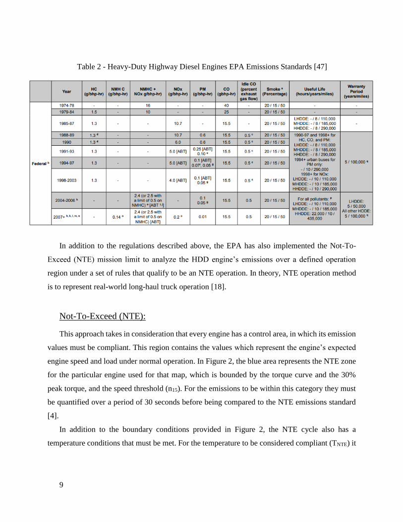
If one looks at Figure 20 the temperature follows the expected trend – higher temperatures at
higher vehicle speeds and power fraction. However, the dataset does have its highest value located
at bin 12 (0-10mph and power fraction>50%) which also represents the lowest value for NOx rate
(g/bhp-hr). According to Figure 19, this is the same bin that only contains one window. This
indicates that the lack of data in that bin category may not be representative of the actual operation
condition. This point even though it’s supposedly compliant to the regulation didn’t even fall inside
of the NTE zone.
Figure 20 - Original Data Post-SCR Exhaust Temperature (oC) Bin - Monthly
Page 44
35
Figure 22 - Original Data NOx (g) Bin - Monthly
Figure 21 - Original Data Power (bhp) Bin - Monthly
Page 45
36
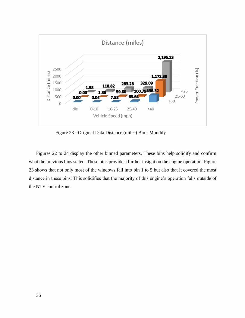
Figures 22 to 24 display the other binned parameters. These bins help solidify and confirm
what the previous bins stated. These bins provide a further insight on the engine operation. Figure
23 shows that not only most of the windows fall into bin 1 to 5 but also that it covered the most
distance in these bins. This solidifies that the majority of this engine’s operation falls outside of
the NTE control zone.
Figure 23 - Original Data Distance (miles) Bin - Monthly
Page 46
37
NOx Stable
The data replaced with NaNs account for 3.48% of the sensor’s operation. The NOx stable data
display similar results to the original dataset. Its values are almost the same values as the original
at bins at medium to high speed (>25mph). Due to the reduction, the values where the vehicle
speed is less than 25mph the bins start diverting from the original dataset. Those bins probably
contained the majority of the noise that was removed and replaced with NaNs. However, according
to Figure 18 the majority of these bins that display a difference are not in NTE region. In addition,
the low NOx value found in bin 12 was removed thus it can be attributed to the issues described
in the original data section.
Figure 24 - Stable Reduction Method NOx Data (g/bhp-hr) Bin - Monthly
Page 47
38
EWMA
Figure 25 - EWMA Method (EWF=0.1) NOx Data (g/bhp-hr) Bin - Monthly
Figure 26 - EWMA Method (EWF=0.25) NOx Data (g/bhp-hr) Bin - Monthly
Page 48
39
When applying the EWMA method three different EWF values were used to see how it affects
the overall dataset. These binning only displays a noticeable difference between each other at the
lower power fraction and lower vehicle speeds. It is to be expected that at the lower bins (<25%
and <25mph) the NOx rate to be higher, since it the aftertreatment system at those bins usually
haven’t met the desired temperature yet. In Figure 19 it shows that bin 12 only had one value in it,
and this value for NOx mass, as shown in Figure 22, is the lowest non-zero value in the bin set.
Therefore the lack of data in that bin and the very low value in the only data in that set is probably
the reason why the data in that bin doesn’t follow the trend of the rest of the data. In fact, this point
could be the result from errors in the system making that point not relevant to the overall engine’s
operation. Overall, all the bsNOx bins that went through reduction displayed higher values at the
lower speed/lower power fraction and lower values at higher speed/higher power fraction.
Weekly
For the weekly binning set, the data shown next is the data collected between April 8th and
April 14th of 2018. The data for the week timeframe displayed similar results to the data from the
month analysis. Therefore, most of the bin graphs for this section can be found in Appendix A.
Figure 27 - EWMA Method (EWF=0.35) NOx Data (g/bhp-hr) Bin - Monthly
Page 49
40
Figure 28 - Original Data NOx (g/bhp-hr) Bin - Weekly
Figure 29 - Original Data NTE Bin - Weekly
Page 50
41
Table 7 – Total Duration Summary - Weekly
Weekly Data
Total Duration (sec) 160455
Total NTE Duration (sec) 24540
NTE Time % 15.29
Total NOx (g) 87.31
Total Distance (miles) 1332.68
By reducing the time frame the bin that displayed issues in the monthly dataset (bin 12) was
removed. The bsNOx bin follows a similar trend to the monthly dataset, however the weekly set
displayed less values in the NTE zone (less than 16% of its weekly operation has fallen in the NTE
zone). The highest NTE count, similarly to the monthly dataset, is located on bin 10, which in this
dataset also displays the lowest bsNOx value. The value in this bin is very close to the regulation
which could indicate compliance, considering that only 31% of the values in that bin fell inside
the NTE zone. In addition, the higher bsNOx value in bin 2 could be attributed to the larger amount
of windows in that category when compared to the other adjacent bins. This dataset shows that by
reducing the dataset to almost a quarter of the original set the bins still display reasonable patterns.
However, the overall bsNOx values are higher than the monthly dataset. This could be attributed
to this particular week that was selected, meaning that in different weeks the vehicle could have
higher operation weeks than others.
Page 51
42
NOx Stable
The data replaced with NaNs accounts for 3.00% of the sensor’s operation, almost the same
amount as the monthly result. Similar to the previous results, the bsNOx data diverted from the
original the most at lower speed/power bins. This indicates that the data that was removed has
definitely affected the overall results. Considering that the original dataset contained several spots
in which the NOx (ppm) values were negative by removing them a difference in the data should
be expected, just as Figure 30 shows. This set actually displayed less of a shift than the monthly
dataset.
Figure 30 - Stable Reduction Method NOx Data (g/bhp-hr) Bin - Weekly
Page 52
43
EWMA
Figure 31 - EWMA Method (EWF=0.1) NOx Data (g/bhp-hr) Bin - Weekly
Figure 32 - EWMA Method (EWF=0.25) NOx Data (g/bhp-hr) Bin - Weekly
Page 53
44
For the weekly dataset, once more the increase in EWF caused an increase of bsNOx in the
overall dataset which is concentrated on the lower power fraction (<25%). When comparing this
method to the NOx stable method, all the EWFs displayed lower values in the bsNOx bin than the
other method. In fact, the EWF of 0.1 showed the closest values to the original dataset.
Daily
For the daily binning set, the data shown next is the data collected on April 10th 2018. The
following results are from the original raw dataset, before any data reduction was applied.
Similarly to the weekly data the daily data displayed similar results to the data from the monthly
analysis. Therefore, most of the bin graphs for this section can be found in Appendix B.
Table 8 - Total Duration Summary - Daily
Daily Data
Total Duration (sec) 22320
Total NTE Duration (sec) 3120
NTE Time % 13.98
Total NOx (g) 9.83
Total Distance (miles) 153.60
Figure 33 - EWMA Method (EWF=0.35) NOx Data (g/bhp-hr) Bin - Weekly
Page 54
45
Figure 34 - Original Data NOx (g/bhp-hr) Bin - Daily
Figure 35 - Original Data NTE Bin - Daily
Page 55
46
Once more the daily dataset displayed a similar distribution to the previous time frames. This
indicates that this method could be used to analyze an engine’s operation. The main difference in
this dataset relies on the fact that the majority of its operation happened at idle. The bins that fall
into this category are outside the NTE control zone. In addition, the NTE zone has even less points
than the previous methods (~14% of the total operation) which is a result of the majority of its
operation happening outside the NTE boundary and this being the shortest dataset among all sets
analyzed.
NOx Stable
The data replaced with NaNs account for 3.11% of the sensor’s operation, only slightly less
than the monthly operation. Compared to the previous sets, in this one the bsNOx had the largest
difference between the original values and reduced values that went through the Stable NOx
method. Several of the bins were greatly reduced, but none of the bins reached NOx regulation
value. This is most likely due to the amount of data available for this time segment, making it more
susceptible to cold start effects. The dataset probably had more transient values than the previous
datasets analyzed.
Figure 36 - Stable Reduction Method NOx Data (g/bhp-hr) Bin - Daily
Page 56
47
EWMA
Figure 37 - EWMA Method (EWF=0.1) NOx Data (g/bhp-hr) Bin - Daily
Figure 38 - EWMA Method (EWF=0.25) NOx Data (g/bhp-hr) Bin - Daily
Page 57
48
The daily dataset follows the same trend for the EWF as the previous timeframes. The
reduction didn’t affect the data enough to cause the points to become compliant or to increase
enough to the point in which it exceeds regulation.
Limitations
From the results described above, the binning method displays certain limitations. For
instance, regardless of the time frame selected for analysis the method does indicate a certain type
of vehicle vocation. From the binned set one could say that this vehicle does mostly long transit
operation. This indicates that this is most likely not a stop and go driving cycle vehicle. However,
the data doesn’t indicate anything more specific about its vocation. Only that the majority of its
operation happen at >25mph bins. In addition, during cold start periods the sensor doesn’t record
data. This indicates that the NCPT method may not be the most representative method for vehicles
that have mostly stop and go driving operation.
Figure 39 - EWMA Method (EWF=0.35) NOx Data (g/bhp-hr) Bin - Daily
Page 58
49
5. Conclusions and Recommendations
Conclusion
When implementing the NTE in this project not all the boundary conditions for the control
zone were included. This means that several of the points that did fall inside of the zone may be
removed once all the restrictions are applied. In addition, the protocol for NTE control zone
requires the points to be continuously compliant with the boundary conditions for a period of 30
seconds. Both of these considerations most likely will reduce the number of points in the NTE
zone, which more than likely will affect the emission in those bins. In addition, by only using the
load parameters in the NTE zone the majority of the data was already excluded from the zone.
This is due to the 30% peak torque and rated power restriction. Most of this engine’s operation fell
inside the <25% power fraction bins. Therefore, the binning method without the NTE zone
restrictions provide a much better insight of the engine’s operation.
Another option would be to reduce the number of bins by removing the power fraction
parameter and only use vehicle speed activity for binning – broken into urban, regional, and
highway. However, this could cause an unbalanced shift in the emission’s profile. For urban
activity the high emission in the lower power fraction bins would be distributed across the bins
where it displays much lower emissions. In the other hand, for the highway bins the data wouldn’t
have such an impactful outcome compared to keeping it into separate bins. This is because the
values in those bins are much closer than the bins in the urban activity. As for the idle bins, the
only bin that is populated is the <25% rated power bin. These bins’ differences become more
apparent when the data is reduced to a shorter time period, such as the daily data analysis. In those
cases the data in the bins differ from each other to their respective vehicle activity range. This
indicates that if all bins in the idle section were combined the value would be representative of the
idle operation emissions where not the same can be said for the urban operation. The bins
schematics could be potentially reduced in certain sections but not all without changing the data
distribution. In addition, the NCPT binning method shows the most suitable representation for all
vehicle’s vocation. In cases in which a vehicle displays stop and go operation, the NOx data would
become more transient and therefore more unstable. Due to cold start sensor limitation, in these
cases the binning wouldn’t best represent the vehicles emission profile.
Page 59
50
Regarding the data reduction method, the results show that by modifying the raw dataset the
bsNOx bins do display changes. This indicates a need to properly reduce the data in order to
remove the points in which there’s noise. When studying emissions one should expect positive
values under 1000 ppm [43] and low non-negative concentration values. This is because when the
true concentration is near zero the sensor may display negative values. However, the results in this
study display several values above 1000 ppm as well as several values in the negative zone (<-
100ppm). These values if not addressed can affect the emission results and considering how low
the regulation is for bsNOx (0.2 g/bhp-hr) the difference in the values could be extremely
impactful. The NOx stable reduction did method removed all the points that exceeded reasonable
expectation. However, replacing them with interpolated value may not be the most representative
option. Meanwhile, the EWMA method provides the option to smooth the original data without
the removal of any data points. The key issue with this method is selecting the best EWF. All the
reducing methods analyzed only affected the data significantly at locations were the emissions
exceed the regulation by more than double. Therefore, when binning the data, even for a short
duration, the reduction method does not impact the overall engine’s emission significantly if it’s
to be compared to the emissions regulations.
Recommendations
With the development of better EATS technology and more strict regulations there’s a need to
find a way to ensure that these engines are following regulations. In addition, the current methods
to analyze the engine operation are outdated and are not representative of the current vehicles’
driving cycles. Therefore, a further analysis of this method should be performed. Some of the
recommendations for the future projects related to this topic include:
1. Perform NTE calculations including all the boundary parameters as well as increase the
time averaging to 30 seconds increment.
2. Perform the NTE NOx emissions calculations for the points that do fall inside the control
zone.
3. Investigate the possibility of changing the NTE boundaries, such as reducing minimum
torque/power or minimum NTE event duration, in order to decrease the amount of excluded
data.
Page 60
51
4. Study how the noise and error from other parameters, such as the exhaust flow, affect the
bsNOx emission.
5. Investigate the impact of the duration of the windows (Δt) on the emission’s profile and
NTE.
6. Investigate data by comparing the onboard sensors to PEMS when applying the NOx
control approach.
7. Further analyze more possibilities of combing certain bin categories.
8. Study other possible parameters that could assist the analysis of the engine’s operation,
such as fuel consumption.
Page 61
52
6. References
[1] J. B. Heywood, Internal Combustion Engine Fundamentals, New York: McGraw-
Hill, 1988.
[2] U.S. Department of Tranportation, "2017 Pocket Guide to Large Truck and Bus
Statistics," June 2017. [Online]. Available:
https://www.fmcsa.dot.gov/sites/fmcsa.dot.gov/files/docs/safety/data-and-
statistics/81121/2017-pocket-guide-large-truck-and-bus-statistics-final-508c-0001.pdf.
[Accessed 21 January 2019].
[3] B. Demirgok, Development of an Emissions Monitoring Methodology Using On-
Board NOx Sensors and Revision to Current In-Use Emissions Regulatory Protocols,
Morgantown: WVU, 2018.
[4] R. P. Pondicherry, Effects of boundary parameters on the Work-Based Window
(WBW) and Not-to-Exceed (NTE) in-use emissions quantification methods, Morgantown:
West Virginia, 2017.
[5] CARB, "CARB gets “REAL” to further cut pollution from diesel and gas vehicles,"
CARB, 15 November 2018. [Online]. Available: https://ww2.arb.ca.gov/news/carb-gets-
real-further-cut-pollution-diesel-and-gas-vehicles. [Accessed 22 April 2019].
[6] History.com, "Automobile History," A&E Televiosion Networks, 21 August 2018.
[Online]. Available: https://www.history.com/topics/inventions/automobiles. [Accessed
28 January 2019].
[7] R. Dundon, "Photos: L.A.'s mid-century smog was so bad, people thought it was a
gas attack," TIMELINE, 23 May 2018. [Online]. Available: https://timeline.com/la-
smog-pollution-4ca4bc0cc95d. [Accessed 29 January 2019].
[8] EPA, "Evolution of the Clean Air Act," United States Environmental Protection
Agency, [Online]. Available: https://www.epa.gov/clean-air-act-overview/evolution-
clean-air-act. [Accessed 29 January 2019].
[9] "The Air Quality Act of 1967," Journal of the Air Pollution Control, vol. 18, no. 2,
pp. 62-71, 1968.
[10] California Air Resources Board, "California Air Resources Board," California Air
Resources Board, 11 May 2018. [Online]. Available:
https://www.arb.ca.gov/msprog/hdlownox/hdlownox.htm. [Accessed 12 December
2018].
[11] V. Akkerman, Fundamentals of Combustion, Morgantown: West Virginia
University, 2018.
[12] EPA, "Technical Bulletin: Nitrogen Oxides (NOx), Why and How They are
Controlled," November 1999. [Online]. Available: Technical Bulletin: Nitrogen Oxides
(NOx), Why and How They are Controlled. [Accessed 22 January 2019].
[13] EPA, "Control of Air Pollution From Heavy-Duty Engines," Code of Federal
Regulations, vol. 60, no. 169, pp. 45580-45604, 1995.
Page 62
53
[14] U.S EPA, "Nitrogen Dioxide (NO2) Pollution," U.S EPA, 13 October 2017. [Online].
Available: https://www.epa.gov/no2-pollution/basic-information-about-
no2#What%20is%20NO2. [Accessed 18 April 2019].
[15] M. K. Khair and H. Jääskeläinen, "Emission Formation in Diesel Engines," 2015.
[16] Diesel Technology Forum, "Diesel Technology Forum," [Online]. Available:
https://www.dieselforum.org/about-clean-diesel/what-is-scr#. [Accessed 12 December
2018].
[17] H. Kannisto, "Volvo Penta," Volvo, November 2017. [Online]. Available:
http://nordicblog.volvopenta.com/exhaust-aftertreatment-system-cleaning-process-
exhausts/. [Accessed 12 December 2018].
[18] DieselNet, "NTE (Not-To-Exceed) Testing," DieselNet, October 2016. [Online].
Available: https://www.dieselnet.com/standards/cycles/nte.php. [Accessed 1 April
2019].
[19] A. Thiruvengadam, Heavy-Duty Vehicle Emissions Exhaust Aftertreatment System
and Emissions, Morgantown: West Virginia University, 2018.
[20] CAMBUSTION, "CLD Principles," CAMBUSTION, [Online]. Available:
https://www.cambustion.com/products/cld500/cld-principles. [Accessed 22 March
2019].
[21] M. Gautam, W. C. Riddle, G. J. Thompson, D. K. Carder, N. N. Clark, D. W. Lyons
and C. Lyond, Measurement of Brake-Specific NOx Emissions using Zirconia Sensors
for In-Use, On-Board Heavy-Duty Vehicle Applications, Nevada: SAE International,
2002.
[22] MEMBRAPOR, "Electrochemical Gas Sensors," MEMBRAPOR, 2019. [Online].
Available: http://www.membrapor.ch/electrochemical-gas-sensors/. [Accessed 25
March 2019].
[23] P. J. Popp, G. A. Bishop and D. H. Stedman, "Development of a High-Speed
Ultraviolet Spectrometer for Remote Sensing of Mobile Source Notric Oxide
Emissions," Journal of the Air & Waste Management Association, vol. 49, no. 12, pp.
1463-1468, 2011.
[24] J.-L. Tirpitz, D. Pöhler, N. Bobrowski, B. Christenson, J. Rüdiger, S. Schmitt and U.
Platt, "Non-dispersive UV Absorption Spectroscopy: A Promising New Approach for in-
situ Detection of Sulfur Dioxide," Frontiers in Earth Science, 13 March 2019. [Online].
Available: https://www.frontiersin.org/articles/10.3389/feart.2019.00026/full.
[Accessed 20 April 2019].
[25] J. Tu, "Portable Emission Measurement System (PEMS)," [Online]. Available:
https://www.cert.ucr.edu/events/pems2011/13_Jesse%20Tu.pdf. [Accessed 13 March
2019].
[26] W. J. Miller, T. Durbin, K. Johnson and D. Cocker, "Evaluation of Portable
Emissions Measurement Sustems (PEMS) for Inventory Purposes and the Not-To-
Exceed Heavy-Duty Diesel Engine Regulation," University of California, Sacramento,
2006.
Page 63
54
[27] S. Carstens and W. A. Majewski, "NOx Sensors," DieselNet, October 2018. [Online].
Available: https://www.dieselnet.com/tech/sensors_nox.php. [Accessed 31 January
2019].
[28] A. Thiruvengadam, S. Pradhan, B. Demirgok, M. Besch, P. Thiruvengadam and D.
Carder, Evaluation of In-Use Emissions Using On-Board NOx Sensors on Heavy-Duty
Diesel Trucks, Long Beach: WVU, 2017.
[29] A. Thiruvengadam, M. Besch, B. Demirgok and D. Carder, Heavy-Duty OBD:
Evaluation of NOx Control Performance Tracking Parameter, Garden Grove: West
Virginia University, 2018.
[30] A. Frobert, S. Raux, C. Yann and E. Jeudy, About Cross-Sensitivities of NOx Sensors
in SCR Operation, SAE International, 2013.
[31] EPA, On-Board Diagnostic (OBD) Regulations and Requirements: Questions and
Answers, U.S. Environmental Protection Agency, 2003.
[32] CARB, California Code of Regulations Title 13 Section 1971.1, Sacramento: CARB,
2016.
[33] Code of Federal Regulations, "40 CFR 86.1806-17," 28 April 2014. [Online].
Available: https://www.law.cornell.edu/cfr/text/40/86.1806-17. [Accessed 12 March
2019].
[34] B. Shade, D. Carder, G. Thompson and M. Gautam, A Work-Based Window Method
for Calculating In-Use Brake-Specific NOx Emissions of Heavy-Duty Diesel Engines,
Morgantown: SAE International, 2008.
[35] California Air Resources Board, "Heavy-Duty Low NOx Program Workshop," 23
January 2019. [Online]. Available: file:///C:/Users/recastiglionialveste/Desktop/03-
HDIUT_WS01232019.pdf. [Accessed 15 April 2019].
[36] H. Lohninger, "Fundamentals of Statistics," Epina, 08 10 2012. [Online]. Available:
http://www.statistics4u.com/fundstat_eng/cc_moving_average.html. [Accessed 10 April
2019].
[37] J. Ellis, Heavy Duty OBD Program Update, SAE International, 2017.
[38] A. Milton, "Simple, Exponential, and Weighted Moving Averages," the balance, 31
December 2018. [Online]. Available: https://www.thebalance.com/simple-exponential-
and-weighted-moving-averages-1031196. [Accessed 5 February 2019].
[39] L. Smith, "Exponentially Weighted Moving Average," COMPOSE, 8 March 2017.
[Online]. Available: https://www.compose.com/articles/metrics-maven-calculating-an-
exponentially-weighted-moving-average-in-postgresql/. [Accessed 2019 February
2019].
[40] Breaking Down Finance, "Exponentially Wrighted Moving Average," Breaking
Down Finance, [Online]. Available: https://breakingdownfinance.com/trading-
strategies/technical-analysis/exponentially-weighted-moving-average/. [Accessed 21
March 2019].
[41] Emission Compliance, Automotive Regulations, "Workshop for 2018 HD OBD
Regulations Update," California Air Resources Board, El Monte, 2017.
Page 64
55
[42] AnswerMiner, "Histogram - The Ultimate Guide of Binning," AnswerMiner, 1
August 2017. [Online]. Available: https://www.answerminer.com/blog/binning-guide-
ideal-histogram. [Accessed 12 December 2018].
[43] DieselNet, "Gaseous Emissions," Ecopoint Inc., January 2018. [Online]. Available:
https://www.dieselnet.com/tech/emi_gas.php. [Accessed 2 February 2019].
[44] A. Thiruvengadam, Heavy-Duty Vehicle Emissions Engine Technology and
Emissions, Morgantown: West Virginia University, 2018.
[45] T. Montes, Heavy Duty OBD Program Update, Barcelona: SAE International, 2018.
[46] Figaro, "Electrochemical-type Operating System," Figaro USA Inc., 2018. [Online].
Available: https://www.figaro.co.jp/en/technicalinfo/principle/electrochemical-
type.html. [Accessed 11 March 2019].
[47] EPA, "Heavy-Duty Highway Compression-Ignition Engines and Urban Buses:
Exhaust Emissions Standards," EPA, March 2016. [Online]. Available:
https://nepis.epa.gov/Exe/ZyPDF.cgi?Dockey=P100O9ZZ.pdf. [Accessed 10 February
2019].
Page 65
56
Appendix A: Bin Plots for Week Dataset
Figure 40 - Original Data Post-SCR Exhaust Temperature (oC) Bin - Weekly
Figure 41 - Original Data Power (bhp) Bin - Weekly
Page 66
57
Figure 43 - Original Data NOx (g) Bin - Weekly
Figure 42 - Original Data Distance (miles) Bin - Weekly
Page 67
58
Figure 44 - Original Data Bin Count - Weekly
Page 68
59
Appendix B: Bin Plots for Daily Dataset
Figure 45 - Original Data Post-SCR Exhaust Temperature (oC) Bin - Daily
Figure 46 - Original Data Power (bhp) Bin - Daily
Page 69
60
Figure 47 - Original Data NOx (g) Bin - Daily
Figure 48 - Original Data Distance (miles) Bin - Daily
Page 70
61
Figure 49 - Original Data Bin Count - Daily