Evaluation and comparison of flow number calculation methods
Mahmoud Ameria ,b∗, Amir Hossein Sheikhmotevalia and Arash Fasihpoura
aSchool of Civil Engineering, Iran University of Science and Technology, Narmak, Tehran, Iran; bCenterof Excellence for PMS, Transportation and Safety, Transportation Research Institute, Tehran, Iran
(Received 4 November 2012; accepted 19 November 2013 )
The objective of this research study is to evaluate and compare several methods to be used incalculating the onset of tertiary flow (referred to as flow number (FN) parameter) for asphaltmixtures. The FN indicates the onset of shear deformation in asphalt mixtures, which is asignificant parameter in evaluating rutting in the field; however, its variability has limited itsimplementation. The FN is obtained from the repeated load permanent deformation laboratorytest. To evaluate and compare the methods, permanent deformation data from tests performedon 12 mixtures were analysed in terms of within- and between-sample variability and theirability to determine whether a tertiary stage was reached or not. The results showed that formodified and unmodified asphalt mixtures the Francken model has lowest variability and maybe used as the final method for calculating FN.
Keywords: flow number; variability; permanent deformation; EVA
1. IntroductionIn the past few years, major research was conducted under the National Cooperative HighwayResearch Program (NCHRP) Project 9-19 “Superpave Support and Performance Models Manage-ment”, which was aimed to recommend a “Simple Performance Test (SPT)” to complement theSuperpave volumetric mixture design method. The results from the NCHRP 9-19 project recom-mended three candidate SPT tests: flow time (FT), flow number (FN) and dynamic modulus |E∗|tests (Witczak, Kaloush, Pellinen, El-Basyouny, & Von Quintus, 2002). The majority of interesthas centred around dynamic modulus with primary efforts on refining associated predictive equa-tions. However, it is felt by many that an additional test should be employed in conjunction withdynamic modulus within the Mechanistic-empirical pavement design guide (Witczak et al., 2002).Currently, there is interest in incorporating FN as the additional test method (Kvasnak, Robinette,& Williams, 2007). When comparing |E∗| with FN, researchers indicated that FN can be betterfor differentiating the rutting performance and quality of asphalt mixtures (Bhasin, Button, &Chowdhury, 2004; Mohammad, Wu, Obulareddy, Cooper, & Abadie 2006; Zhou & Scullion,2003). Faheem, Bahia, and Ajideh (2005) showed that FN is an important mixture property andhas a strong correlation to the Traffic Force Index, which represents densification loading by thetraffic during its service life. The mixture ranking order obtained from the FN tests was con-sistent with the use of those mixtures in the field while the |E∗| test could not correctly rankthe permanent deformation characteristics for those mixtures (Mohammad et al., 2006). A studyconducted by Witczak (2007) demonstrated that a good correlation exists between the FN andfield rutting performance. However, concerns regarding the variability of the FN may present a
challenge in its implementation. The FN has been reported to show a high degree of variability,as indicated by Mohammad et al. They report coefficient of variation (CV) from unconfined FNtests between 22.3% and 58.4% (Mohammad et al., 2006). In a study conducted by Bhasin et al.(2004) CV for FN tests on 12 different mixtures were reported to range between 4% and 81%.The establishment of a unified method for determining the FN from the axial repeated load testdata can help limit this variability, and contribute to extend its use as a mixture rutting indicator.Currently, no standard FN calculation method is widely accepted. Researchers have been trying todiscover a well-defined FN method through different kinds of approaches. Their efforts led to thedevelopment of several excellent methods. However, these methods need to be more refined inorder to improve its user friendliness to engineers, researchers and even students. These modelsor methods are presented and summarised in Tables 1 and 2. The first objective of this paperis to evaluate these methods. The model should be applicable to both mixtures produced withunmodified and modified bitumens. Also it should be able to determine whether a tertiary stagewas reached or not (Biligiri, Kaloush, Mamlouk, & Witczak, 2007). The second objective of thispaper is to compare these methods in terms of variability to find a best method for FN calculation.
2. FN testingTesting conditions. Testing conditions for the FN test have not been standardised (Bonaquist,2010). Two approaches for this testing have emerged from recent research. NCHRP Project 9-33has recommended using an unconfined test with the following conditions (Christensen, 2012):
• Repeated axial stress: 600 kPa.• Temperature: 50% reliability high-performance grade temperature, without traffic or speed
adjustments, from LTPPBind3.1 at a depth of 20 mm for surface courses and the top of thelayer for intermediate and base courses.
• Air void content: 7.0 ± 0.5%.
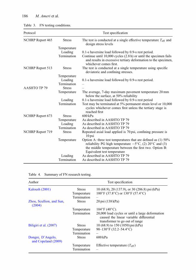
For tests conducted using these conditions, criteria have been developed for various traffic levelsand were presented in Christensen (2012). The second approach is the confined test that is cur-rently being used in NCHRP Project 9-30A in the development of an improved rutting model forasphalt concrete (Von Quintus, Mallela, Bonaquist, Schwartz, & Carvalho, 2012). This test usesa confining pressure of 69 kPa and a repeated deviatoric stress of 483 kPa. The Project 9-30Aresearchers believe that confining pressure is needed to differentiate the difference in rutting resis-tance for various mixture types. As it is presented in the NCHRP Report 580, the FN not only isuseful to indicate the start of the tertiary stage of permanent deformation in asphalt mixes, but alsoprovides the required parameters to accurately predict the field rut depth based on mechanistic andfundamental laboratory test and regression data (Witczak, 2007). Thus, the validity and enormouspotential of this performance test are once again demonstrated. The FN test protocol developedin NCHRP Project 9-19 recommended testing at the effective pavement temperature using eitherunconfined tests with axial stress between 70 and 210 kPa or confined tests with confining pressurebetween 35 and 210 kPa and deviator stress between 490 and 980 kPa (Witczak, 2007). Unfortu-nately, the conditions for conducting the FN test were not fully standardised in NCHRP Project9-19 (Yu & Shen, 2011). Using the effective pavement temperature and the range of stress lev-els recommended in NCHRP Project 9-19 resulted in many mixtures not exhibiting flow within10,000 cycles, the recommended maximum number of load cycles. A 10,000-cycle test requires2.8 h; therefore, researchers using the FN test arbitrarily increased either the temperature, devia-toric stress or both to ensure that flow would occur in the mixtures within 10,000 load cycles (Yu &Shen, 2011). Available most important conditions for FN testing are summarised in Tables 3 and 4.
184 M. Ameri et al.
Table 1. Description of different FN calculation methods.
Model name Model equation Description
Three-stage model Primary stage: FN = NSTεp = aN b, N < NPS The method consists of first
determining the NPS usingthe power-law model tofit the curve with specifieddeviation. Then, a linearregression model is used toobtain the FN by evaluatingthe absolute ratio of themodel’s intercept to the currentmaximum adjusted cumulativepermanent deformation
a, b, c, d and f are material constants; NPS and NST are number of load repetitions corresponding to theinitiation of the secondary stage and tertiary stage, respectively and εPS and εST are permanent straincorresponding to the initiation of the secondary and tertiary stage, respectively (Zhou, 2004)
FNest model εp = 1β
[− ln
(1 − N
γ
)]1/αFN = γ
[1 − exp
(1α
− 1)]
First, the range of load cycles tobe used for fitting the proposedmodel is determined then themodel parameter values arecalculated
β, α and γ are probability distribution parameters (Archilla, 2007)
Francken model εp(N ) = AN B + C(eDN − 1) The regression constants areobtained. The cycle numberwhere the second derivative ofthe composite model changedfrom a negative value to apositive value was reported asthe FN
A, B, C and D are the regression constants (Biligiri et al., 2007)
Hoerl model dεpdN = (A × BN × N C) The regression constants are
obtained. The cycle numberwhere the first derivative ofthe Hoerl model changed froma negative value to a positivevalue was reported as the FN
A, B and C are the regression constants (Li, Lee, & Hwang, 2010)
Creep curve analyse. The FN test is based on the results from repeated loading and unloadingof an asphalt concrete specimen where the permanent deformation of the specimen is recordedas a function of load cycles. There are three stages of flow that occurred during the test definedas: primary, secondary and tertiary flow. Under primary flow, there is a decrease in the strainrate with time. Then, with continuous repeated load application, the next phase is the secondaryflow state, which is characterised by a relatively constant strain rate. The material enters tertiaryflow when the strain rate begins to increase dramatically as the test progresses. There are severaloutput parameters that result from performing the repeated load test; e.g. FN, microstrain at FN,total cycles to reach a certain amount of strain and total strain accumulated at the end of specific
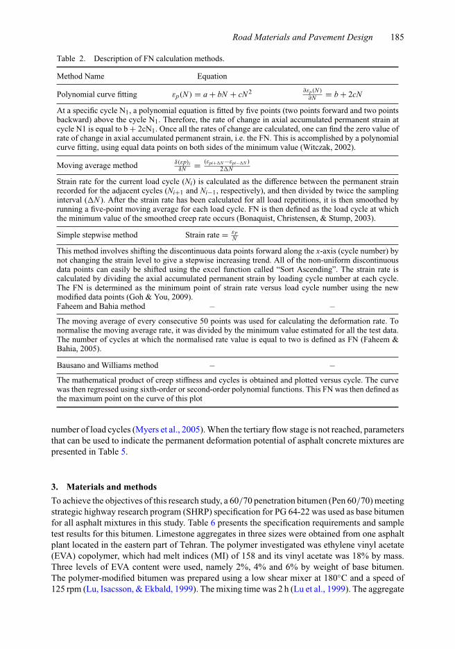
At a specific cycle N1, a polynomial equation is fitted by five points (two points forward and two pointsbackward) above the cycle N1. Therefore, the rate of change in axial accumulated permanent strain atcycle N1 is equal to b + 2cN1. Once all the rates of change are calculated, one can find the zero value ofrate of change in axial accumulated permanent strain, i.e. the FN. This is accomplished by a polynomialcurve fitting, using equal data points on both sides of the minimum value (Witczak, 2002).
Moving average method δ(εp)iδN = (εpi+�N −εpi−�N )
2�N
Strain rate for the current load cycle (Ni) is calculated as the difference between the permanent strainrecorded for the adjacent cycles (Ni+1 and Ni−1, respectively), and then divided by twice the samplinginterval (�N ). After the strain rate has been calculated for all load repetitions, it is then smoothed byrunning a five-point moving average for each load cycle. FN is then defined as the load cycle at whichthe minimum value of the smoothed creep rate occurs (Bonaquist, Christensen, & Stump, 2003).
Simple stepwise method Strain rate = εPN
This method involves shifting the discontinuous data points forward along the x-axis (cycle number) bynot changing the strain level to give a stepwise increasing trend. All of the non-uniform discontinuousdata points can easily be shifted using the excel function called “Sort Ascending”. The strain rate iscalculated by dividing the axial accumulated permanent strain by loading cycle number at each cycle.The FN is determined as the minimum point of strain rate versus load cycle number using the newmodified data points (Goh & You, 2009).Faheem and Bahia method – –
The moving average of every consecutive 50 points was used for calculating the deformation rate. Tonormalise the moving average rate, it was divided by the minimum value estimated for all the test data.The number of cycles at which the normalised rate value is equal to two is defined as FN (Faheem &Bahia, 2005).
Bausano and Williams method – –
The mathematical product of creep stiffness and cycles is obtained and plotted versus cycle. The curvewas then regressed using sixth-order or second-order polynomial functions. This FN was then defined asthe maximum point on the curve of this plot
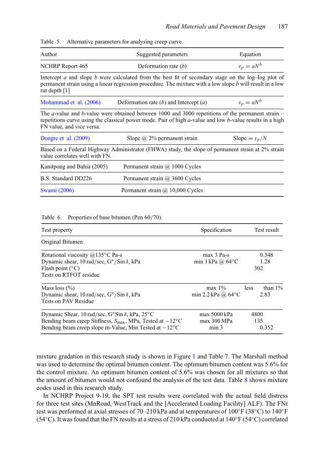
number of load cycles (Myers et al., 2005). When the tertiary flow stage is not reached, parametersthat can be used to indicate the permanent deformation potential of asphalt concrete mixtures arepresented in Table 5.
3. Materials and methodsTo achieve the objectives of this research study, a 60/70 penetration bitumen (Pen 60/70) meetingstrategic highway research program (SHRP) specification for PG 64-22 was used as base bitumenfor all asphalt mixtures in this study. Table 6 presents the specification requirements and sampletest results for this bitumen. Limestone aggregates in three sizes were obtained from one asphaltplant located in the eastern part of Tehran. The polymer investigated was ethylene vinyl acetate(EVA) copolymer, which had melt indices (MI) of 158 and its vinyl acetate was 18% by mass.Three levels of EVA content were used, namely 2%, 4% and 6% by weight of base bitumen.The polymer-modified bitumen was prepared using a low shear mixer at 180◦C and a speed of125 rpm (Lu, Isacsson, & Ekbald, 1999). The mixing time was 2 h (Lu et al., 1999). The aggregate
186 M. Ameri et al.
Table 3. FN testing conditions.
Protocol Test specification
NCHRP Report 465 Stress The test is conducted at a single effective temperature Teff anddesign stress levels
TemperatureLoading 0.1-s haversine load followed by 0.9-s rest period.
Termination Continue until 10,000 cycles (2.8 h) or until the specimen failsand results in excessive tertiary deformation to the specimen,whichever comes first.
NCHRP Report 513 Stress The test is conducted at a single temperature using specificdeviatoric and confining stresses.
TemperatureLoading 0.1-s haversine load followed by 0.9-s rest period.
Termination –AASHTO TP 79 Stress –
Temperature The average, 7-day maximum pavement temperature 20 mmbelow the surface, at 50% reliability
Loading 0.1-s haversine load followed by 0.9-s rest periodTermination Test may be terminated at 5% permanent strain level or 10,000
cycles whichever comes first unless the tertiary stage isreached first
NCHRP Report 673 Stress 600 kPaTemperature As described in AASHTO TP 79
Loading As described in AASHTO TP 79Termination As described in AASHTO TP 79
Temperature Option A: three test temperatures that are defined as (1) 50%reliability PG high temperature −5◦C, (2) 20◦C and (3)the middle temperature between the first two. Option B:Equivalent test temperature
Loading As described in AASHTO TP 79Termination As described in AASHTO TP 79
Table 4. Summary of FN research testing.
Author Test specification
Kaloush (2001) Stress 10 (68.9), 20 (137.9), or 30 (206.8) psi (kPa)Temperature 100◦F (37.8◦C) or 130◦F (57.4◦C)Termination –
Zhou, Scullion, and Sun,(2004)
Stress 20 psi (138 kPa)
Temperature 104◦F (40◦C).Termination 20,000 load cycles or until a large deformation
caused the linear variable differentialtransformer to go out of range
Biligiri et al. (2007) Stress 10 (68.9) to 150 (1050) psi (kPa)Temperature 90–130◦F (32.2–54.4◦C)Termination –
Dongre, D’Angelo,and Copeland (2009)
Stress 600 kPa
Temperature Effective temperature (Teff )Termination –
Road Materials and Pavement Design 187
Table 5. Alternative parameters for analysing creep curve.
Author Suggested parameters Equation
NCHRP Report 465 Deformation rate (b) εp = aN b
Intercept a and slope b were calculated from the best fit of secondary stage on the log–log plot ofpermanent strain using a linear regression procedure. The mixture with a low slope b will result in a lowrut depth [1]
Mohammad et al. (2006) Deformation rate (b) and Intercept (a) εp = aN b
The a-value and b-value were obtained between 1000 and 3000 repetitions of the permanent strain –repetitions curve using the classical power mode. Pair of high a-value and low b-value results in a highFN value, and vice versa.
Based on a Federal Highway Administrator (FHWA) study, the slope of permanent strain at 2% strainvalue correlates well with FN.
Kanitpong and Bahia (2005) Permanent strain @ 1000 Cycles
B.S. Standard DD226 Permanent strain @ 3600 Cycles
Swami (2006) Permanent strain @ 10,000 Cycles
Table 6. Properties of base bitumen (Pen 60/70).
Test property Specification Test result
Original Bitumen
Rotational viscosity @135◦C Pa-s max 3 Pa-s 0.348Dynamic shear, 10 rad/sec, G∗/Sin δ, kPa min 1 kPa @ 64◦C 1.28Flash point (◦C) 302Tests on RTFOT residue
Mass loss (%) max 1% less than 1%Dynamic shear, 10 rad/sec, G∗/Sin δ, kPa min 2.2 kPa @ 64◦C 2.83Tests on PAV Residue
Dynamic Shear, 10 rad/sec, G∗Sin δ, kPa, 25◦C max 5000 kPa 4800Bending beam creep Stiffness, Smax, MPa, Tested at −12◦C max 300 MPa 135Bending beam creep slope m-Value, Min Tested at −12◦C min 3 0.352
mixture gradation in this research study is shown in Figure 1 and Table 7. The Marshall methodwas used to determine the optimal bitumen content. The optimum bitumen content was 5.6% forthe control mixture. An optimum bitumen content of 5.6% was chosen for all mixtures so thatthe amount of bitumen would not confound the analysis of the test data. Table 8 shows mixturecodes used in this research study.
In NCHRP Project 9-19, the SPT test results were correlated with the actual field distressfor three test sites (MnRoad, WestTrack and the [Accelerated Loading Facility] ALF). The FNrtest was performed at axial stresses of 70–210 kPa and at temperatures of 100◦F (38◦C) to 140◦F(54◦C). It was found that the FN results at a stress of 210 kPa conducted at 140◦F (54◦C) correlated
well with the rutting resistance of the mixtures used in the experimental sections at MnRoad,WestTrack and the ALF. Therefore, a test temperature of 140◦F (54◦C) and a stress level of 30 psi(210 kPa) were selected for this research study (Mohammad et al., 2006; Swami, 2006). Anunconfined test mode was used. This test was conducted for 20,000 load cycles or until a largedeformation caused the linear variable differential transformers to go out of range as recommended
Road Materials and Pavement Design 189
by Zhou et al. (2004). In this research study, the FN test conducted on 12 asphalt mixtures asmentioned in Table 8.
4. Results and discussion4.1. Evaluation of different FN methods4.1.1. Results of three-stage methodGraphical representation. The procedure described in Table 1 was used to determine FN values.Sample of this method to determine the FN is shown in Figure 2.
Analysis of results. In this present research study, for calculating FN using the three-stagemethod, a computer program was developed via Macro in Excel software. Tables 9 and 10 showprimary and secondary stage parameters according to the three-stage method. Table 11 showsFN values determined using the three-stage method for all asphalt mixtures used in this presentresearch study. The control mixture failed around 11,695 cycles (average value) of load, whilethe MEVA2 (average value) failed around 17,343 cycles. The MEVA4 and MEVA6 mixturesexhibited no sign of failure indicating that these mixtures are better in comparison with the othermixtures. As shown in the last column of Table 11, the CV in FN values was relatively high forthe control mixture and reduces considerably for the MEVA2 mixture.
Evaluation of the method. These results show that the three-stage method is able to determinewhether a tertiary stage was reached or not and is applicable to both mixtures produced withunmodified and modified bitumens and work better for modified mixtures.
4.1.2. Results of the FNest methodGraphical representation. The procedure described in Table 1 was used to determine FN values.Sample of this method to determine the FN is shown in Figure 3.
Figure 2. Graphical representation of the three-stage method.
190 M. Ameri et al.
Table 9. The three-stage model parameters: primary stage.
Primary stage
εp = aN b
Mixture Replicate ID a CV (%) b CV (%)
Control 1 0.14 46 0.26 212 0.30 0.193 0.40 0.18
MEVA2 1 0.11 102 0.27 382 0.87 0.123 0.22 0.22
MEVA4 1 0.47 10 0.08 32 0.53 0.073 0.57 0.07
MEVA6 1 0.37 35 0.08 292 0.33 0.093 0.18 0.13
Table 10. The three-stage model parameters: secondary stage.
Secondary stage
εp = εPS + c(N − NPS)
Mixture Replicate ID εPS CV (%) c CV (%) NPS CV (%)
Analysis of results. Table 12 shows the FNest method parameters for all asphalt mixtures usedin this present research study. Solver add-in included in MS Excel was utilised for determiningmodel parameters. The control and MEVA2 mixtures are rut susceptible as they flowed beforethe completion of 10,000 cycles. The MEVA4 and MEVA6 are not rut susceptible because theydid not flow till the end of 20,000 cycles. As shown in the last column of Table 12, the CV inFN values was relatively high for the control mixture and reduces considerably for the MEVA2mixture.
Evaluation of the method. These results show that the FNest method is able to determine whethera tertiary stage was reached or not and is applicable to both mixtures produced with unmodifiedand modified bitumens and work better for modified mixtures.
Road Materials and Pavement Design 191
Table 11. The three-stage model parameters: the tertiary stage.
Tertiary stage
εp = εST + d(ef (N−NST ) − 1)
Mixture Replicate ID εST CV (%) d CV (%) f CV (%) NST CV (%)
Figure 3. Graphical representation of the FNest method.
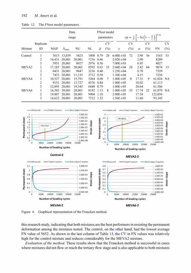
4.1.3. Results of the Francken methodGraphical representation. The procedure described in Table 1 was used to determine FN values.Sample of this method to determine the FN is shown in Figure 4.
Analysis of results. Table 13 shows Francken model parameters, the FN value of individualsamples and percent of CV for all asphalt mixtures used in this present research study. High FNis desired for a rut-resistant mixture. Both MEVA4 and MEVA6 mixtures showed very high FNvalues (FN > 20, 000) under the test condition of compressive stress at 210 kPa (30 psi) used in
192 M. Ameri et al.
Table 12. The FNest model parameters.
Data FNest model
range parameters εp = 1β
[− ln
(1 − N
γ
)]1/α
Replicate CV CV CV CVMixture ID MAP Nmax NU NL β (%) γ (%) α (%) FN (%)
Figure 4. Graphical representation of the Francken method.
this research study, indicating that both mixtures are the best performers in resisting the permanentdeformation among the mixtures tested. The control, on the other hand, had the lowest averageFN value of 5652. As shown in the last column of Table 13, the CV in FN values was relativelyhigh for the control mixture and reduces considerably for the MEVA2 mixture.
Evaluation of the method. These results show that the Francken method is successful in caseswhere mixtures did not flow or reach the tertiary flow stage and is also applicable to both mixtures
Road Materials and Pavement Design 193
Table 13. The Francken model parameters.
Francken model parametersεp (N ) = AN B + C
(eDN − 1
)
Replicate CV CV CV CV CVMixtures ID A (%) B (%) C (%) D (%) FN (%)
produced with unmodified and modified bitumens and work better for modified mixtures. Theregression results and the predicted model indicate excellent fit of the data, for all three stages,with excellent statistical goodness of fit parameters.
4.1.4. Results of the Hoerl methodGraphical representation. The procedure described in Table 1 was used to determine FN values.Sample of this method to determine the FN is shown in Figure 5.
Analysis of results. Table 14 shows the Hoerl model parameters for all asphalt mixtures usedin this present research study. As shown in the last column of Table 14, the CV in FN values wasrelatively high for the control mixture and reduces considerably for the MEVA2 mixture.
Evaluation of the method. These results show that the Hoerl method is able to determine whethera tertiary stage was reached or not and is applicable to both mixtures produced with unmodifiedand modified bitumens and work better for modified mixtures
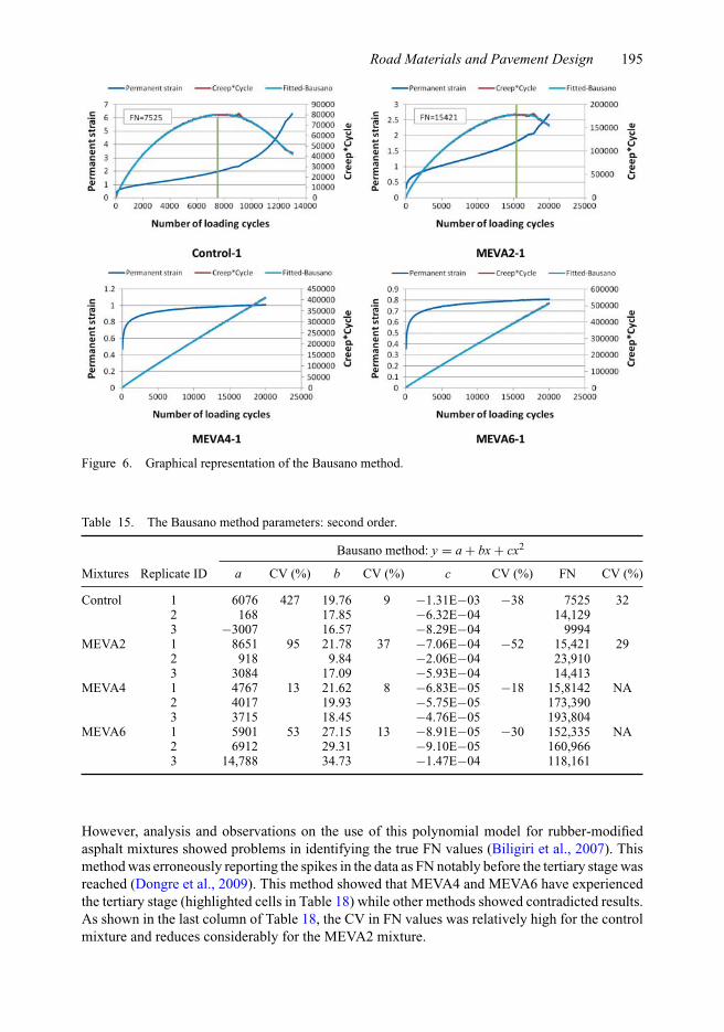
4.1.5. Results of the Bausano methodGraphical representation. The procedure described in Table 2 was used to determine FN values.Sample of this method to determine the FN is shown in Figure 6.
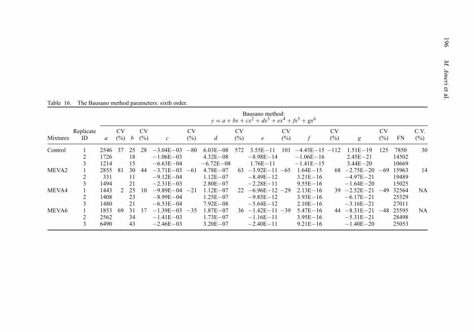
Analysis of results. Bausano indicated that a second polynomial regression provides accuracyand precision of measuring the FN similar to the sixth-order polynomial regression. As shown inTable 15, second-order polynomial function shows that specimen MEVA2-2 has FN of 23,910> 20, 000 and hence no tertiary stage while sixth-order polynomial function shows that specimenMEVA2-2 has FN of 19,489. As shown in the last column of Table 16, the CV in FN valueswas relatively high for the control mixture and reduces considerably for the MEVA2 mixturemoreover compared with second-order polynomial function, sixth-order polynomial functionshows lower CV.
Evaluation of the method. These results show that the Bausano six-order polynomial functionis able to determine whether a tertiary stage was reached or not and is applicable to both mixturesproduced with unmodified and modified bitumens and work better for modified mixtures.
194 M. Ameri et al.
Figure 5. Graphical representation of the Hoerl method.
Table 14. The Hoerl model parameters.
Hoerl model parametersdεp
dN= (
A × BN × N C)
Mixtures Replicate ID A CV (%) B CV (%) C CV (%) FN CV (%)
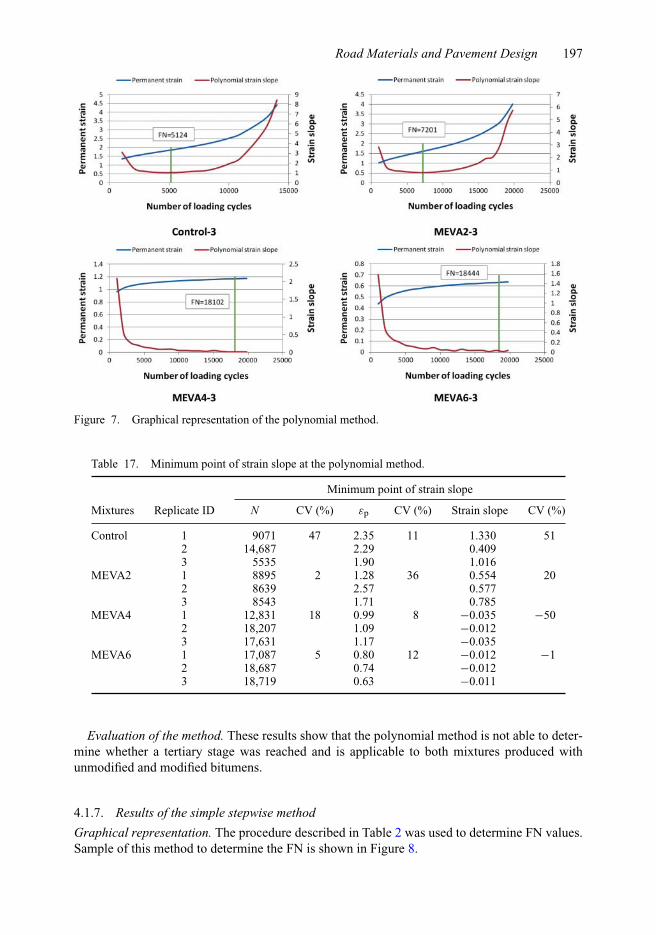
4.1.6. Results of polynomial methodGraphical representation. The procedure described in Table 2 was used to determine FN values.Sample of this method to determine the FN is shown in Figure 7.
Analysis of results. Tables 17 and 18 show the polynomial method parameters for all asphaltmixtures used in this present research study. This method was found to be very sensitive to noisein the data and identifies erroneous FN results, especially for modified mixtures (Dongre et al.,2009). This method works well for most conventional asphalt mixtures (Biligiri et al., 2007).
Road Materials and Pavement Design 195
Figure 6. Graphical representation of the Bausano method.
Table 15. The Bausano method parameters: second order.
Bausano method: y = a + bx + cx2
Mixtures Replicate ID a CV (%) b CV (%) c CV (%) FN CV (%)
However, analysis and observations on the use of this polynomial model for rubber-modifiedasphalt mixtures showed problems in identifying the true FN values (Biligiri et al., 2007). Thismethod was erroneously reporting the spikes in the data as FN notably before the tertiary stage wasreached (Dongre et al., 2009). This method showed that MEVA4 and MEVA6 have experiencedthe tertiary stage (highlighted cells in Table 18) while other methods showed contradicted results.As shown in the last column of Table 18, the CV in FN values was relatively high for the controlmixture and reduces considerably for the MEVA2 mixture.
196M
.Am
erietal.
Table 16. The Bausano method parameters: sixth order.
Evaluation of the method. These results show that the polynomial method is not able to deter-mine whether a tertiary stage was reached and is applicable to both mixtures produced withunmodified and modified bitumens.
4.1.7. Results of the simple stepwise methodGraphical representation. The procedure described in Table 2 was used to determine FN values.Sample of this method to determine the FN is shown in Figure 8.
198 M. Ameri et al.
Table 18. The polynomial method parameters.
Polynomial method parameters
Regressioncoefficient: y = a + bx + cx2
Mixtures Replicate ID a CV (%) b CV (%) c CV (%) FN CV (%)
Figure 8. Graphical representation of the simple stepwise method.
Analysis of results. Table 19 shows FN values determined using the simple stepwise methodfor all mixtures used in this present research study. As shown by Goh and You (2009), this methodhas good relationship with the three-stage method. Therefore, the simple stepwise method maybe used instead of the three-stage model. The three-stage model has more complicated theory andcalculation process. As shown in the last column of Table 19, the CV in FN values was relativelyhigh for the control mixture and reduces considerably for the MEVA2 mixture.
Evaluation of the method. This method could estimate a better FN of modified asphalt mixtureand is able to determine whether a tertiary stage was reached or not.
Road Materials and Pavement Design 199
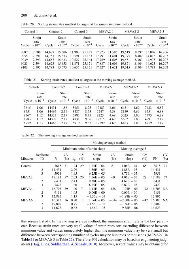
Table 19. The simple stepwise method parameters.
Simple stepwise method
Minimum point of strain slope
Replicate CV CV Strain CV CVMixtures ID N (%) εp (%) slope (%) FN (%)
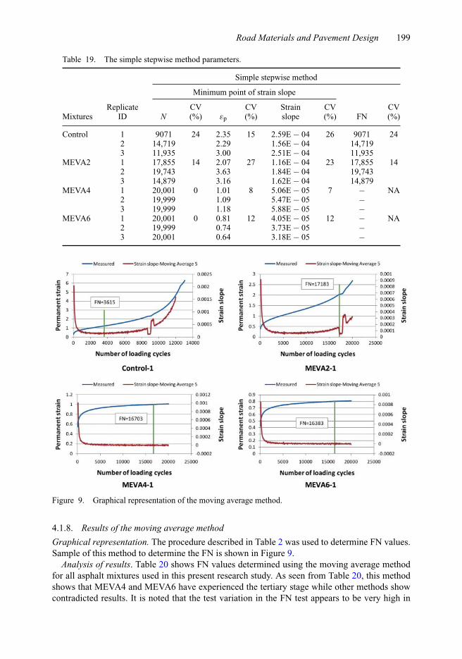
Figure 9. Graphical representation of the moving average method.
4.1.8. Results of the moving average methodGraphical representation. The procedure described in Table 2 was used to determine FN values.Sample of this method to determine the FN is shown in Figure 9.
Analysis of results. Table 20 shows FN values determined using the moving average methodfor all asphalt mixtures used in this present research study. As seen from Table 20, this methodshows that MEVA4 and MEVA6 have experienced the tertiary stage while other methods showcontradicted results. It is noted that the test variation in the FN test appears to be very high in
200 M. Ameri et al.
Table 20. Sorting strain rates smallest to largest at the simple stepwise method.
this research study. In the moving average method, the minimum strain rate is the key param-eter. Because strain rates are very small values if strain rates sort ascending difference betweenminimum value and values immediately higher than the minimum value may be very small butdifference between corresponding number of cycles may be hundreds or thousands (MEVA2-1 inTable 21 or MEVA6-3 in Table 22). Therefore, FN calculation may be based on engineering judg-ments (Hajj, Ulloa, Siddharthan, & Sebaaly, 2010). Moreover, several values may be obtained for
Road Materials and Pavement Design 201
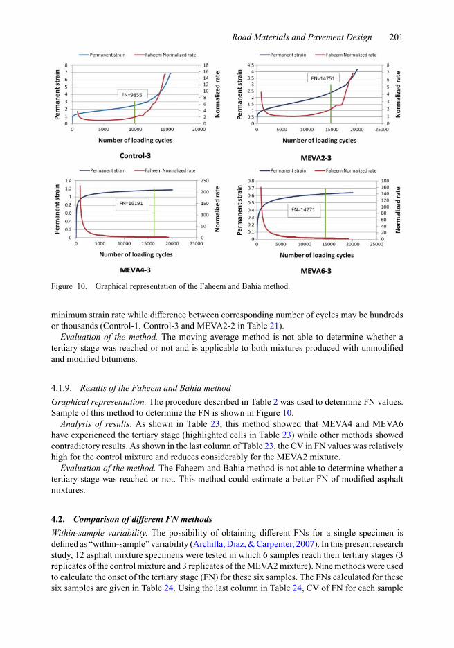
Figure 10. Graphical representation of the Faheem and Bahia method.
minimum strain rate while difference between corresponding number of cycles may be hundredsor thousands (Control-1, Control-3 and MEVA2-2 in Table 21).
Evaluation of the method. The moving average method is not able to determine whether atertiary stage was reached or not and is applicable to both mixtures produced with unmodifiedand modified bitumens.
4.1.9. Results of the Faheem and Bahia methodGraphical representation. The procedure described in Table 2 was used to determine FN values.Sample of this method to determine the FN is shown in Figure 10.
Analysis of results. As shown in Table 23, this method showed that MEVA4 and MEVA6have experienced the tertiary stage (highlighted cells in Table 23) while other methods showedcontradictory results. As shown in the last column of Table 23, the CV in FN values was relativelyhigh for the control mixture and reduces considerably for the MEVA2 mixture.
Evaluation of the method. The Faheem and Bahia method is not able to determine whether atertiary stage was reached or not. This method could estimate a better FN of modified asphaltmixtures.
4.2. Comparison of different FN methodsWithin-sample variability. The possibility of obtaining different FNs for a single specimen isdefined as “within-sample” variability (Archilla, Diaz, & Carpenter, 2007). In this present researchstudy, 12 asphalt mixture specimens were tested in which 6 samples reach their tertiary stages (3replicates of the control mixture and 3 replicates of the MEVA2 mixture). Nine methods were usedto calculate the onset of the tertiary stage (FN) for these six samples. The FNs calculated for thesesix samples are given in Table 24. Using the last column in Table 24, CV of FN for each sample
202 M. Ameri et al.
Table 23. The Faheem and Bahia method parameters.
Faheem and Bahia method
Mixtures Replicate ID Minimum of strain slope CV (%) FN CV (%)
Control 1 1.44E−04 35 8127 302 6.97E−05 14,3353 1.04E−04 9855
or “within-sample” variability was plotted (Figure 11). The observed “within-sample” variabilitydue to the use of different methods fell between 30% and 50%, as illustrated in Figure 11 andshows that for a single specimen different FN calculation methods do not converge to a singlevalue and there is high variability between them.
Between-sample variability. The “between-sample” variability is variability in the determina-tion of FN for the same replicates when one calculation method is used. Table 24 shows CV of FNmethods for control and MEVA2 mixtures (between-sample variability) and plotted in Figure 12.As seen from Figure 12, for the control asphalt mixture, simple stepwise and Francken meth-ods and for the MEVA2 mixture the Francken method have lowest CV; all methods work betterfor MEVA2 than the control mixture as lower variability was obtained for the MEVA2 mixture(Figure 12). For all asphalt mixtures, the Francken model has lowest variability and therefore issuggested as the final method for calculating FN.
Road Materials and Pavement Design 203
Table 24. FN of asphalt mixtures.
Replicate Three Simple Moving CVMixture ID stage Francken FNest Hoerl Polynomial stepwise average Faheem Bausano (%)
4.3. Evaluation of alternative parametersTable 25 presents alternative parameters for all mixtures tested in this research study whetherthe tertiary stage was reached or not. The FN results indicate that control and MEVA2 mixturesexperience tertiary flow. All of the alternative parameters showed that MEVA2 has a better ruttingresistance than the control mixture. In addition, the FN results indicate that MEVA4 and MEVA6may not reach tertiary flow or at least not in a practical amount of time or before 5% strain.While the total strain accumulated at the end of specified number of cycles shows that MEVA6is more rut resistant than MEVA4, deformation rate shows that MEVA4 has better resistance. Inaddition, the current proposed protocol to shorten FN test time based on predicting FN based onthe permanent deformation slope at 2% strain may not be applicable to these mixtures. Thus, more
204 M. Ameri et al.
Table 25. Calculation of alternative parameters.
Total strain accumulated at the end Deformationof number of cycles rate
Replicate Slope @Mixtures ID 1000 3600 10,000 2%Strain b(1000–3000) b
research is needed in order to establish a proper alternative parameter-related modified mixtures,especially in the case of high polymer content.
5. ConclusionsIn this present research study, nine methods were used to calculate the onset of the tertiary stage.The following conclusions were obtained.
• Three methods polynomial, moving average and Faheem and Bahia are unable to determineoccurrence of the tertiary stage.
• Different FN calculation methods do not have same results for a single specimen and thereis high variability between them.
• The high variations in FN calculation may cause difficulties in developing the final designcriteria for its use in a Superpave mix design.
• For all asphalt mixtures, the Francken model has the lowest variability and therefore issuggested as the final method for calculating FN.
ReferencesArchilla, A. R., Diaz, L. G., & Carpenter, S. H. (2007). Proposed method to determine the flow number
in bituminous mixtures from repeated axial load tests. Journal of Transportation Engineering, 133,610–617.
Bhasin, A., Button, J. W., & Chowdhury, A. (2004). Evaluation of simple performance tests on hot-mixasphalt mixtures from south central United States. Transportation Research Record: Journal of theTransportation Research Board, 1891(1), 174–181.
Road Materials and Pavement Design 205
Biligiri, K. P., Kaloush, K. E., Mamlouk, M. S., & Witczak, M. W. (2007). Rational modeling of tertiaryflow for asphalt mixtures. Transportation Research Record: Journal of the Transportation ResearchBoard, 2001(1), 63–72.
Bonaquist, R. F., Christensen, D. W., & Stump, W. (2003). NCHRP Report 513 Simple performance testerfor superpave mix design: First-article development and evaluation. Transportation Research Board.Retrieved from http://www.trb.org/Main/Blurbs/153587.aspx
Bonaquist, R. (2010). Wisconsin mixture characterization using the Asphalt Mixture Performance Tester(AMPT) on historical aggregate structures (WHRP 09-03). Madison, WI: Wisconsin Department ofTransportation.
Christensen, D. (2012). A manual for the design of hot mix asphalt with commentary (NCHRP Report 673).Dongre, R., D’Angelo, J., & Copeland, A. (2009). Refinement of flow number as determined by the Asphalt
Mixture Performance Tester for use in routine QC/QZ practice. Washington, DC: TransportationResearch Board (TRB).
Faheem, A. F., Bahia, H. U., & Ajideh, H. (2005). Estimating results of a proposed simple performancetest for hot-mix asphalt from Superpave gyratory compactor results. Transportation Research Record:Journal of the Transportation Research Board, 1929(1), 104–113.
Goh, S. W., & You, Z. (2009). A simple stepwise method to determine and evaluate the initiation of tertiaryflow for asphalt mixtures under dynamic creep test. Construction and Building Materials, 23(11), 3398–3405.
Hajj, E. Y., Ulloa, A., Siddharthan, R., & Sebaaly, P. E. (2010). Estimation of stress conditions for theflow number simple performance test. Transportation Research Record: Journal of the TransportationResearch Board, 2181(1), 67–78.
Kaloush, K. E. (2001). Simple performance test for permanent deformation of asphalt mixtures. (PhDDissertation). Department of Civil and Environmental Engineering, Arizona State University, Tempe,Arizona.
Kanitpong, K., & Bahia H. (2005). Relating adhesion and cohesion of asphalts to the effect of mois-ture on laboratory performance of asphalt mixtures. Transportation Research Record: Journal of theTransportation Research Board 1901(1), 33-43.
Kvasnak, A., Robinette, C. J., & Williams, R. C. (2007). Statistical development of a flow number predictiveequation for the mechanistic-empirical pavement design guide. Transportation research board 86thannual meeting. Transportation Research Board; 2007. p. 18.
Li, Q., Lee, H. J., & Hwang, E. Y. (2010). Characterization of permanent deformation of asphalt mixturesbased on shear properties. Transportation Research Record: Journal of the Transportation ResearchBoard, 2181(1), 1–10.
Lu, X., Isacsson, U., & Ekblad, J. (1999). Rheological properties of SEBS, EVA and EBA polymer modifiedbitumens. Materials and Structures, 32(2), 131–139.
Mohammad, L. N., Wu, Z., Obulareddy, S., Cooper, S., & Abadie, C. (2006). Permanent deformationanalysis of hot-mix asphalt mixtures with simple performance tests and 2002 mechanistic-empiricalpavement design software. Transportation Research Record: Journal of the Transportation ResearchBoard, 1970(1), 133–142.
Myers, L. A., Gudimettla, J., Paugh, C., D Angelo, J., Gohkale, S., & Choubane, B. (2005). Evaluation ofperformance data from repeated load test. Proceedings of the annual conference, Canadian TechnicalAsphalt Association.
Swami, V. (2006). Performance testing of crumb rubber modified hot mix asphaltic concrete (TechnicalReport, FHWA/TX-06/0-4821-2).
Von Quintus, H., Mallela, J., Bonaquist, R., Schwartz, C., & Carvalho, R. (2012). Calibration of ruttingmodels for structural and mix design (NCHRP report 719). Washington, DC: Transportation ResearchBoard of the National Academies.
Witczak, M. W. (2007). Specification criteria for simple performance tests for rutting: Volume I: Dynamicmodulus (E∗) and volume II: Flow number and flow time (NCHRP report 580). Washington, DC:Transportation Research Board of the National Academies.
Witczak, M., Kaloush, K., Pellinen T., El-Basyouny, M., & Von Quintus, H. (2002). Simple performancetest for superpave mix design (NCHRP Report 465). National Cooperative Highway Research Programreport.
Yu, H., & Shen, S. (2011). An investigation of dynamic modulus and flow number properties of asphaltmixtures in Washington State. Pullman, WA: Washington Department of Transportation.
Zhou, F., & Scullion, T. (2003). Preliminary field validation of simple performance tests for permanentdeformation: case study. Transportation Research Record: Journal of the Transportation ResearchBoard, 1832(1), 209–216.
Zhou, F., Scullion, T., & Sun, L. (2004). Verification and modeling of three-stage permanent deformationbehavior of asphalt mixes. Journal of Transportation Engineering, 130, 486–494.