Evaluation of an Analog Accelerator for Linear Algebra

Yipeng Huang∗, Ning Guo†, Mingoo Seok†, Yannis Tsividis†, and Simha Sethumadhavan∗∗Department of Computer Science, †Department of Electrical Engineering

Columbia UniversityNew York, NY, USA

{yipeng@cs., ng2364@, mgseok@ee., tsividis@ee., simha@cs.}columbia.edu

Abstract—Due to the end of supply voltage scaling and theincreasing percentage of dark silicon in modern integratedcircuits, researchers are looking for new scalable ways toget useful computation from existing silicon technology. Inthis paper we present a reconfigurable analog acceleratorfor solving systems of linear equations. Commonly perceiveddownsides of analog computing, such as low precision andaccuracy, limited problem sizes, and difficulty in programmingare all compensated for using methods we discuss. Based ona prototyped analog accelerator chip we compare the perfor-mance and energy consumption of the analog solver against anefficient digital algorithm running on a CPU, and find that theanalog accelerator approach may be an order of magnitudefaster and provide one third energy savings, depending on theaccelerator design. Due to the speed and efficiency of linearalgebra algorithms running on digital computers, an analogaccelerator that matches digital performance needs a largesilicon footprint. Finally, we conclude that problem classesoutside of systems of linear equations may hold more promisefor analog acceleration.

Keywords-accelerator architectures; analog-digital integratedcircuits; analog computers; linear algebra.

I. INTRODUCTION

In anticipation of the post-Moore’s-law era of computing,there has been a scramble to either discover devices whichcan replace CMOS transistors, or to otherwise find waysto harness performance and efficiency from existing silicontechnologies. Analog computing has been touted as one ap-proach to address these challenges without the need for noveldevice technologies. For those familiar with the principlesand history of analog computing, the expectations regardinganalog computing’s promise range from extremely positiveto extremely negative.

Analog computing has many alluring properties: broadly,analog computing abandons digital representation of num-bers, and also abandons step-by-step operation typical inmodern computing. Much of research throughout computerarchitecture is in the line of breaking historical abstractionswhich hold back performance and efficiency of comput-ers. Among the remaining abstractions yet to be brokenare binary representation and discrete-time operation. Inthis regard analog computing may unleash untapped usesfor existing CMOS technology. Arguments against analogcomputing include hardware design difficulty, low precision,

limited scalability, programming difficulty, and even lowperformance improvements.

Analog computing effectively solves nonlinear ordinarydifferential equations, which frequently appear in cyber-physical systems workloads, with higher performance andefficiency compared to digital systems [1]–[4]. The analog,continuous-time output of analog computing is especiallysuited for embedded systems applications where actuatorscan use such results directly.

This work explores using analog computing in commoditymainstream computing systems. The main difference be-tween the embedded application and this work is that, herewe strive to use analog computing for solving a class ofproblems typically handled in digital computing (specifi-cally, systems of linear equations as opposed to differentialequations). Furthermore, we consider how analog computingcan be leveraged if the outputs cannot be directly fed toactuators and have to be processed further digitally.

Towards this goal we present an architecture that al-lows analog computing results to be safely used with con-ventional architectures. The architecture is envisioned asan accelerator-style architecture with the digital processoracting as a host and the analog accelerator acting as aperipheral. Our architecture provides the digital host theability to configure, control, and capture data from ananalog accelerator, and to be able to react when problemsoccur in the course of analog computation. The choice ofproblem that we solve, system of linear equations, sets anextremely high bar for analog computing to challenge asthe importance of this class of problems has led to highlyefficient techniques in modern digital computing.

This work is a study of analog computing in the context ofmodern mainstream computer architecture. Using physicaltiming, power, and area measurements given by Guo et.al. [3], [4], we build a model that predicts the properties oflarger scale analog accelerators. The perceived downsidesof analog computing, such as low precision, and inabilityto sample intermediate results at high frequency, can beovercome. For instance, we find that precision of the resultsobtained from analog computing can be increased arbitrarilyirrespective of the resolution of the analog-to-digital con-verter, and that there is also a way to divide large workloadsinto pieces that enables solution on limited analog hardware.

Data: time, steps, a, b, uinit

Result: evolution of u over time in stepsstepSize← time÷ steps;u← uinit;for step← 0; step < steps; step← step+ 1 do

δ ← a× u+ b;u← u+ stepSize× δ;

endAlgorithm 1: Euler’s method for Equation 1

As such programmability challenges can be overcome withproper support for exceptions and the ability to decomposeand map problems.

On performance and energy metrics, we find that withhigh analog bandwidth, analog acceleration can potentiallyhave 10× faster solution time and 33% lower energy con-sumption compared to a digital general-purpose processor.However, our analysis finds that high bandwidth in analogcomputers comes with high area cost, severely limiting theproblem sizes that can be solved on an analog accelerator ata time. This ultimately limits the benefit of analog computingto this class of problems.

While our findings do not make a strong case for us-ing analog accelerators for this important workload, ourexperience from using analog circuitry to accelerate digitalcomputation provides guidance for future analog workloadsand architectures.

The rest of the paper is organized as follows: Section IIgives background on analog computation and the challengesthat must be overcome in analog acceleration. Section III-Aand III-B presents the microarchitecture and architecturefor an analog accelerator. Section IV discusses problemsand algorithms in scientific computing and how they canbe solved using analog acceleration. Section V comparesanalog and digital computing solving sparse, structured gridproblems. We analyze our empirical results and reviewperceptions about analog computing in Section VI. Sec-tion VII discusses related directions in analog computing.Section VIII concludes.

II. ANALOG COMPUTING BACKGROUND

This section is a tutorial on analog computation. Analogcomputing works by solving systems of ordinary differentialequations (ODEs). We can also solve other types of problemsby transforming them into ODEs. We discuss the mainchallenges that need to be overcome to use an analog ac-celerator in conjunction with a digital computer, on modernworkloads.

A. Solutions to ODEs: Digital and Analog

Analog computers solve ODEs, which state the timederivatives of variables as functions of the variables. Asimple linear first-order ODE has the form:

du

dt= au+ b (1)

dudt

u

a

b

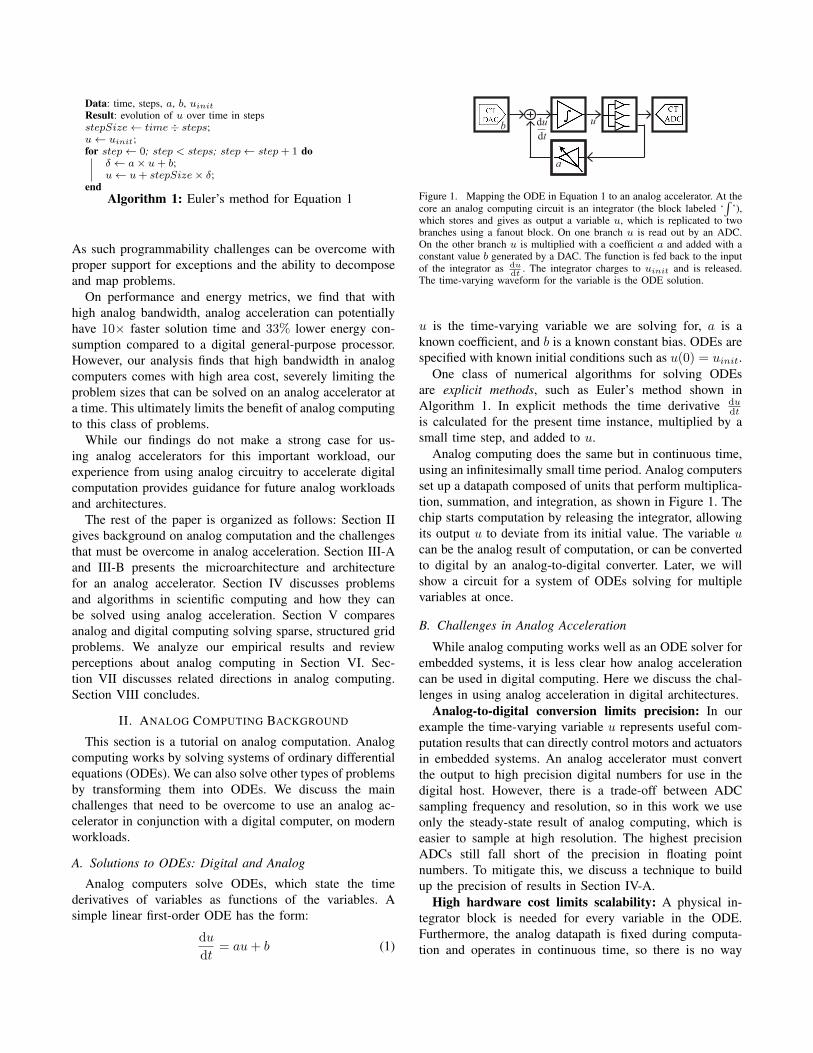
Figure 1. Mapping the ODE in Equation 1 to an analog accelerator. At thecore an analog computing circuit is an integrator (the block labeled ‘

∫’),

which stores and gives as output a variable u, which is replicated to twobranches using a fanout block. On one branch u is read out by an ADC.On the other branch u is multiplied with a coefficient a and added with aconstant value b generated by a DAC. The function is fed back to the inputof the integrator as du

dt. The integrator charges to uinit and is released.

The time-varying waveform for the variable is the ODE solution.

u is the time-varying variable we are solving for, a is aknown coefficient, and b is a known constant bias. ODEs arespecified with known initial conditions such as u(0) = uinit.

One class of numerical algorithms for solving ODEsare explicit methods, such as Euler’s method shown inAlgorithm 1. In explicit methods the time derivative du

dtis calculated for the present time instance, multiplied by asmall time step, and added to u.

Analog computing does the same but in continuous time,using an infinitesimally small time period. Analog computersset up a datapath composed of units that perform multiplica-tion, summation, and integration, as shown in Figure 1. Thechip starts computation by releasing the integrator, allowingits output u to deviate from its initial value. The variable ucan be the analog result of computation, or can be convertedto digital by an analog-to-digital converter. Later, we willshow a circuit for a system of ODEs solving for multiplevariables at once.

B. Challenges in Analog Acceleration

While analog computing works well as an ODE solver forembedded systems, it is less clear how analog accelerationcan be used in digital computing. Here we discuss the chal-lenges in using analog acceleration in digital architectures.

Analog-to-digital conversion limits precision: In ourexample the time-varying variable u represents useful com-putation results that can directly control motors and actuatorsin embedded systems. An analog accelerator must convertthe output to high precision digital numbers for use in thedigital host. However, there is a trade-off between ADCsampling frequency and resolution, so in this work we useonly the steady-state result of analog computing, which iseasier to sample at high resolution. The highest precisionADCs still fall short of the precision in floating pointnumbers. To mitigate this, we discuss a technique to buildup the precision of results in Section IV-A.

High hardware cost limits scalability: A physical in-tegrator block is needed for every variable in the ODE.Furthermore, the analog datapath is fixed during computa-tion and operates in continuous time, so there is no way

to dynamically load variables from and store variables tomain memory. Modern workloads routinely need thousandsof integrators, exceeding area constraints of realistic analogaccelerators. Large-scale problems must be decomposed intosubproblems that can be solved in the analog accelerator.We discuss how sparse systems of linear equations can bedecomposed in Section IV-B.

Different problems need significant reprogramming:Analog computing literature of the 1960s abounds withapplication-specific techniques for simulation and engineer-ing design. However, digital computing has advanced signifi-cantly since the decline of analog computing, and now offersmore flexibility and reliability, even if analog computingtechniques offer high performance and efficiency. For analogacceleration to succeed, it must be able to accelerate acore kernel which is used extensively, without significantreprogramming to support new problems.

In order to address these architectural challenges, inthis work we explore using analog computing to supportsolving sparse linear equations, which commonly arise insolving differential equations. We use the prototype analogaccelerator presented in [3], [4] to validate the approach,and to serve as a basis for quantifying the performance,area cost, and energy efficiency of analog accelerators. Weemphasize that this analog accelerator is designed primarilyas an ODE solver, and is therefore not representative of ananalog accelerator designed as a system of linear equationssolver.

III. A PROTOTYPE ANALOG ACCELERATOR

In this section we describe the microarchitecture of ouranalog accelerator and its hardware/software interface.

A. Analog Accelerator: Microarchitecture

Our research group recently prototyped an analog chipin 65nm CMOS technology [3], [4], shown in Figures 2and 3. The accelerator consists of analog functional unitsconnected with a crossbar. Each chip is organized as fourmacroblocks, each macroblock consisting of one analoginput from off-chip, two multipliers, one integrator, twocurrent-copying fanout blocks, and one analog output to off-chip. Two macroblocks share use of an 8-bit ADC, an 8-bit DAC, and a nonlinear function lookup table (256-deep,8-bit continuous-time SRAM [5]). The chip also includesan interface to receive commands from the main digitalprocessor. In the prototype these commands are receivedover an interface implementing an SPI protocol.

In our analog accelerator, electrical currents representvariables. Fanout current mirrors allow copying variables byreplicating values onto different branches. To sum variables,currents are added together by joining branches. Eight mul-tipliers allow variable-variable and constant-variable multi-plication. The variables can also be subjected to arbitrary

Figure 2. Chip layout diagram reproduced from [3], [4] showing rowsof analog, mixed-signal, and digital components, along with crossbarinterconnect. Each of the four rows of analog components are logicallyorganized as a macroblock. “CT” refers to continuous time. SRAMs areused as lookup tables for nonlinear functions.

Figure 3. Die photo reproduced from [3], [4] of analog computer chipfabricated in 65 nm showing major components. “VGAs” are variable-gainamplifiers. Die area is 3.8mm2.

nonlinear functions, such as sine, signum, and sigmoid withthe SRAM lookup table.

Overflow detection is done using analog voltage compara-tors to detect values exceeding the safe range. We compare areference value (usually the maximum or minimum allowedvalues) to the signal carrying the variable. When a valueexceeds the safe range an exception bit is set in a latchwhose value can be read out during exception checking.

B. Analog Accelerator: Architecture

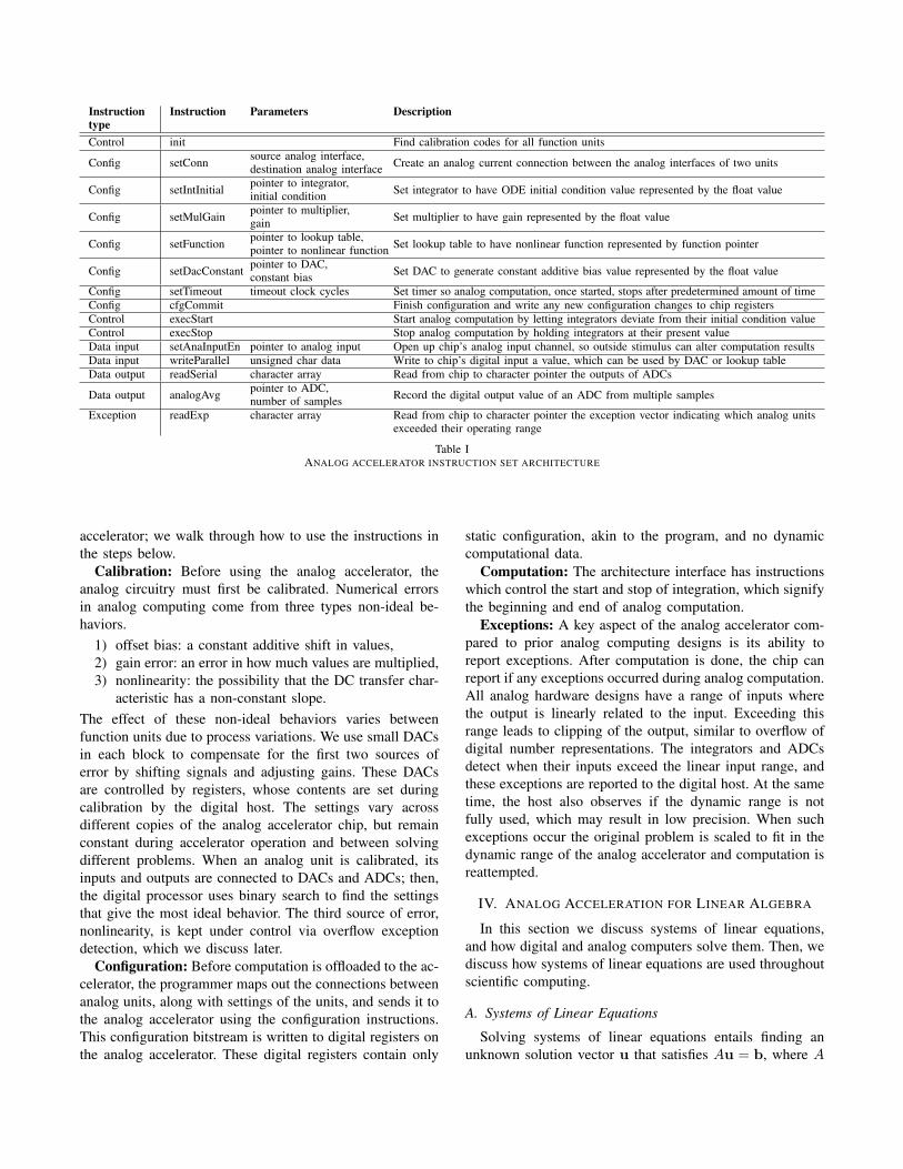
The analog accelerator acts as a peripheral to a digitalhost processor, which provides a configuration for the analogaccelerator, performs calibration, controls computation, andreads out the output values. Table I summarizes the essentialsystem calls and corresponding instructions for the analog

Instructiontype

Instruction Parameters Description

Control init Find calibration codes for all function units

Config setConn source analog interface,destination analog interface Create an analog current connection between the analog interfaces of two units

Config setIntInitial pointer to integrator,initial condition Set integrator to have ODE initial condition value represented by the float value

Config setMulGain pointer to multiplier,gain Set multiplier to have gain represented by the float value

Config setFunction pointer to lookup table,pointer to nonlinear function Set lookup table to have nonlinear function represented by function pointer

Config setDacConstant pointer to DAC,constant bias Set DAC to generate constant additive bias value represented by the float value

Config setTimeout timeout clock cycles Set timer so analog computation, once started, stops after predetermined amount of timeConfig cfgCommit Finish configuration and write any new configuration changes to chip registersControl execStart Start analog computation by letting integrators deviate from their initial condition valueControl execStop Stop analog computation by holding integrators at their present valueData input setAnaInputEn pointer to analog input Open up chip’s analog input channel, so outside stimulus can alter computation resultsData input writeParallel unsigned char data Write to chip’s digital input a value, which can be used by DAC or lookup tableData output readSerial character array Read from chip to character pointer the outputs of ADCs

Data output analogAvg pointer to ADC,number of samples Record the digital output value of an ADC from multiple samples

Exception readExp character array Read from chip to character pointer the exception vector indicating which analog unitsexceeded their operating range

Table IANALOG ACCELERATOR INSTRUCTION SET ARCHITECTURE

accelerator; we walk through how to use the instructions inthe steps below.

Calibration: Before using the analog accelerator, theanalog circuitry must first be calibrated. Numerical errorsin analog computing come from three types non-ideal be-haviors.

1) offset bias: a constant additive shift in values,2) gain error: an error in how much values are multiplied,3) nonlinearity: the possibility that the DC transfer char-

acteristic has a non-constant slope.The effect of these non-ideal behaviors varies betweenfunction units due to process variations. We use small DACsin each block to compensate for the first two sources oferror by shifting signals and adjusting gains. These DACsare controlled by registers, whose contents are set duringcalibration by the digital host. The settings vary acrossdifferent copies of the analog accelerator chip, but remainconstant during accelerator operation and between solvingdifferent problems. When an analog unit is calibrated, itsinputs and outputs are connected to DACs and ADCs; then,the digital processor uses binary search to find the settingsthat give the most ideal behavior. The third source of error,nonlinearity, is kept under control via overflow exceptiondetection, which we discuss later.

Configuration: Before computation is offloaded to the ac-celerator, the programmer maps out the connections betweenanalog units, along with settings of the units, and sends it tothe analog accelerator using the configuration instructions.This configuration bitstream is written to digital registers onthe analog accelerator. These digital registers contain only

static configuration, akin to the program, and no dynamiccomputational data.

Computation: The architecture interface has instructionswhich control the start and stop of integration, which signifythe beginning and end of analog computation.

Exceptions: A key aspect of the analog accelerator com-pared to prior analog computing designs is its ability toreport exceptions. After computation is done, the chip canreport if any exceptions occurred during analog computation.All analog hardware designs have a range of inputs wherethe output is linearly related to the input. Exceeding thisrange leads to clipping of the output, similar to overflow ofdigital number representations. The integrators and ADCsdetect when their inputs exceed the linear input range, andthese exceptions are reported to the digital host. At the sametime, the host also observes if the dynamic range is notfully used, which may result in low precision. When suchexceptions occur the original problem is scaled to fit in thedynamic range of the analog accelerator and computation isreattempted.

IV. ANALOG ACCELERATION FOR LINEAR ALGEBRA

In this section we discuss systems of linear equations,and how digital and analog computers solve them. Then, wediscuss how systems of linear equations are used throughoutscientific computing.

A. Systems of Linear Equations

Solving systems of linear equations entails finding anunknown solution vector u that satisfies Au = b, where A

Time independent PDE

Time dependent PDE

Partial differential equation (PDE)

Parabolic PDE (e.g., heat equation)

Hyperbolic PDE (e.g., wave equation)

Elliptic PDE (e.g., Poisson eq.)

Spatial discretization Spatial discretization

System of ordinary differential equations (ODE)

Explicit time stepping (e.g., RK4, analog)

Implicit time stepping (e.g., backward Euler)

Sparse system of linear equations (SLE)

Direct solvers (e.g., Cholesky, QR, SVD)

Iterative solvers (e.g., CG, analog)

Dense linear eqs. (e.g., optimization)

Nonlinear system of equations

Nonlinear solvers (e.g., Newton’s)

Figure 4. Taxonomy of some classes of problems in scientific compu-tation. Physical phenomena are described as partial differential equations.PDEs are solved by applying appropriate space and time discretizations,converting the continuous problem format into discrete node variables,interrelated by systems of algebraic equations. The dark boxes show steps toconvert or solve problems. One way analog acceleration supports scientificcomputation is by acting as explicit solvers for systems of ODEs [3], [4].This paper focuses on using analog computing as an iterative solver forsparse linear equations.

is a matrix of known coefficients and b is a vector of knownconstant biases. Linear algebra algorithms that solve theseproblems include sparse matrix, dense matrix, structured,and unstructured grid algorithms, and are the bulk of theBerkeley Dwarfs taxonomy [6]. As shown in the bottomlayer of Figure 4, scientific computation workloads mostlysolve sparse linear algebra problems, where variables areloosely interconnected. Machine learning and optimizationproblems frequently solve dense linear algebra problems,where variables have all-to-all connectivity. Performance andefficiency gains in solving linear algebra problems would behighly beneficial.

Linear algebra techniques are categorized as direct anditerative solvers. Direct solvers focus on factoring the matrix,resulting in algorithms that assign correct values to thesolution one element at a time. Notable direct solvers includeCholesky decomposition and Gaussian elimination. The lit-erature on analog computing points out that analog comput-ers are not suitable for direct linear algebra approaches [7].On the other hand, iterative solvers start at an initial guessuinit; the entire solution evolves step-by-step toward thecorrect answer according to an algorithm until the solutionstops changing and is accurate at ufinal. Even if an iterativesolver is stopped short of full convergence, the intermediatesolution still approximately satisfies the original system oflinear equations. Notable iterative solvers include conjugategradients (CG) and steepest gradient descent.

In analog computing, we can imagine the iterative solver

du0

dt

du1

dtu1

u0

-a10

-a00

-a01

-a11

b1

b0

Figure 5. Solving a system of two linear equations with two unknownsin an analog accelerator.

taking smaller steps more frequently, until it is takinginfinitesimally small steps in continuous time. In continuous-time gradient descent, the time derivative of the solutionvector is set to be the gradient pointing in the directionof the correct answer, resulting in the system of ODEs:dudt = b−Au(t). For example, a simple two-variable systemof linear equations would be solved using the system ofODEs:

d

dt

[u0(t)u1(t)

]=

[b0b1

]−[a00 a01a10 a11

] [u0(t)u1(t)

](2)

This ODE can be mapped to analog hardware as shownin Figure 5. As u(t) evolves, the derivative approacheszero so long as A is a positive definite matrix. When thederivative becomes zero, the steady state value of u(t)satisfies the system of linear equations, and can be read outusing ADCs. These techniques were used in early analogcomputers [8]–[14], and have been recently explored insmall scale experiments with analog computation [15]–[18].

In contrast to solving time-varying ODEs, here the analogaccelerator’s ADCs only have to sample the value of thestable output ufinal, which means that sampling frequencyis not a concern. If even higher precision is needed, moresignificant digits can can be obtained from the analog resultby solving more times, each time setting b to be the residual,and scaling the problem up as necessary to fully use thedynamic range of the analog hardware. This procedureis shown in Algorithm 2. The longer sampling period,combined with Algorithm 2, mitigates concerns regardingADC precision described in Section II-B.

Finally we note that imprecise solutions from analogacceleration are still useful in multigrid partial differentialequation solvers. In multigrid PDE solvers, the overallPDE is converted to several linear algebra problems with

Data: A, bResult: uprecise with high precisionuprecise ← 0;residual← b;while ||residual|| > tolerance do

analog accelerator solves Aufinal = residual;uprecise ← uprecise + ufinal;residual← b−Auprecise;

endAlgorithm 2: Building precision in analog result

Figure 6. An example elliptic PDE. The continuously varying field hasbeen discretized into node variables which are solved using linear algebra.

varying spatial resolution. Lower-resolution subproblemsare quickly solved and fed to high-resolution subproblems,aiding the high-resolution problem to converge faster. Thelinear algebra subproblems can be solved approximately.Overall accuracy of the solution is guaranteed by repeatingthe multigrid algorithm. Because perfect convergence is notrequired, less stable, inaccurate, low precision techniques,such as analog acceleration, may also be used to supportmultigrid.

B. Linear Algebra for Elliptic Partial Differential Equations

As shown in Figure 4, elliptic partial differential equationsare a fundamental class of PDEs. This class of problemsis important in physical field simulations, such as fluiddynamics and solid mechanics. While such problems are notintrinsically difficult to solve, they dominate scientific com-putation workloads, and can take significant of computingpower to solve when the problems have high dimensionality,high spatial resolution, and when they must be solved to highaccuracy and precision.

The 2D Poisson elliptic PDE has the form ∂2u∂x2 + ∂2u

∂y2 =b(x, y). The continuous spatial partial derivatives indicatethat u(x, y) varies continuously over 2D space. The problemis discretized into L×L grid points, converting the contin-uous field into node variables. For example, using a 3 × 3grid on the unit square:

u0 u1 u2u3 u4 u5u6 u7 u8

would result in nine node variables in the vector u which

are interrelated according to the system of linear equations:

Au = b

A =1132

4 −1 −1−1 4 −1 −1

−1 4 −1−1 4 −1 −1

−1 −1 4 −1 −1−1 −1 4 −1

−1 4 −1−1 −1 4 −1

−1 −1 4

u = [u0, u1, . . . , u8]

>,b = [b0, b1, . . . , b8]>

The coefficients in the matrix are a result of using a second-order central finite difference stencil. The coefficient valueof 9 in front of A emerges because we discretized the 2Dunit square into thirds on each side. Notice A is sparse,meaning that most coefficients are zero, a result from thefact cells are only related to itself, and to its four neighbors.

In practice, physics simulations using PDEs have millionsof grid points in the vector u, far larger than the problemsizes that can fit in an analog accelerator. Both digitaland analog techniques would subdivide the large grid sizeproblem into smaller linear problems. For example, the 3×32D problem can be solved as a set of three independent 1Dsubproblems:

Asus = bs

As =11h2

4 −1 0−1 4 −10 −1 4

,us =

us0us1us2

,bs =

bs0bs1bs2

,This decomposition temporarily ignores the coefficients thatconnect the 1D problems into a 2D problem. The subprob-lems can be solved separately on multiple accelerators, ormultiple runs of the same accelerator.

Solving the system of equations as block matrices onlyensures that the solution vector us is correct for the subprob-lem. To get overall convergence across the entire problem,the set of subproblems would be solved several times,using a larger iteration across the subproblems. Typically,the larger iteration is an iterative method operating onvectors, and do not have as strong convergence propertiesas iterative methods on individual numbers. Therefore, it isstill desirable to ensure the block matrices are large, so thatmore of the problem is solved using the efficient lower levelsolver.

Using this domain decomposition technique, in conjunc-tion to accuracy boosting and a multigrid algorithm wecan use the analog accelerator to calculate an elliptic PDEsolution as shown in Figure 6. These divide-and-conquer andapproximate computing techniques in solving PDEs miti-gates concerns regarding precision and scalability describedin Section II-B.

V. METHODOLOGY AND EVALUATION

In this section we compare analog and digital computa-tion in terms of performance, hardware area, and energyconsumption, using 2D Poisson PDEs as an example prob-lem. We take into account accuracy, problem size, and thebandwidth of the analog accelerator design.

Accuracy: We compare the analog accelerator and thedigital algorithm running on a CPU at equal solution accu-racy, measured as the error in the solution. This is done bystopping the numerical iteration in the digital version wellshort of machine epsilon provided by high-precision digitalfloating point numbers. The stopping criterion is when noelement in the output vector u changes by more than 1/256of full scale. This is equivalent to the amount of precisionin the output vector that can be obtained from one run ofthe analog accelerator.

Problem size: We vary the total number of grid points inthe problem N = L2, where L is the number of incrementson one side. We compare analog and digital solutions forgrids of up to 2048 points. The relatively small problem sizeis due to the lack of dense data storage for analog variablesin analog accelerators. As a case in point, the fabricatedprototype chip has only four integrators to hold variables.Nonetheless, the chip establishes confidence in using theanalog blocks for computation. Using the validated schemat-ics we build circuit simulations in Cadence R© Virtuoso R©,in order to extrapolate the area and energy consumption oflarger scale analog accelerators.

Bandwidth: The most important parameter in the analogaccelerator design is the analog components’ bandwidth.Increasing the bandwidth of the analog circuit design propor-tionally decreases the solution time, but also increases areaand energy consumption. We do a design space explorationof analog accelerators with different bandwidths.

A. Analog and Digital Computation Time

We compare the time it takes for the analog acceleratorand a digital algorithm to solve a 2D Poisson PDE.

In digital computing, the PDE can be solved using manylinear algebra algorithms. Figure 7 establishes that conjugategradients (CG) has the best convergence rate among classicaliterative methods. The CG algorithm is implemented usingstencils to capture the sparse structure of the matrix, withouthaving to allocate memory for the full matrix, and avoidingiterating through the rows and columns of the matrix. Wemeasure the computation time on single threaded code,running on an Intel Xeon X5550, clocked at 2.67 GHz. Theproblem sizes we tackle are smaller than 2048 total gridpoints, so the program data is entirely resident in the firstlevel cache.

Figure 8 shows that the prototype analog design wouldhave parity in terms of computing speed once it reaches asize of roughly 650 integrators. In Section VI-D we give atheoretical model why the analog computer’s solution time

1.00E-171.00E-151.00E-131.00E-111.00E-091.00E-071.00E-051.00E-031.00E-011.00E+011.00E+03

0 5 10 15 20 25 30 35

L2_n

orm

err

or

iterations

cg steepest sor gs jacobi

Figure 7. Comparison of the convergence rate for a Poisson equation.The L2-norm of the error is plotted against the number of numericaliterations. The numerical algorithms are conjugate gradients, steepestdescent, successive over-relaxation, Gauss-Seidel, and Jacobi iterations.We see CG converges to a solution limited by the precision of doubleprecision floating point numbers the quickest. The problem is discretizedusing finite differences with 16 points over three dimensions, for a totalof 4096 grid points. Boundary condition u(x, y, z) = 1.0 for the planex = 0, u(x, y, z) = 0.0 otherwise.

0

200

400

600

800

0 200 400 600 800 1000

conv

erge

nce

time

(s)

total grid points

digital CG analog 20KHz Linear (analog 80KHz projection)

Figure 8. Comparison of time taken to converge to equivalent precision,for an analog accelerator and a CPU. The time needed to converge isplotted against the total number of grid points N = L2. The convergencetime for an analog solution is measured from simulations of larger analogaccelerator circuits based on the prototyped hardware. We give the projectedthe solution time for an 80 KHz bandwidth analog accelerator design. Theconvergence time for the digital comparison is the software runtime on asingle CPU core.

scales linearly with respect to the problem size, measuredin grid points. An analog accelerator with 650 integratorsoccupies about 150 mm2, accounting for integrators, mul-tipliers, current mirrors, DACs, and ADCs; this is smallerthan desktop CPU die sizes.

B. Choice of ADC Precision and Analog Bandwidth

In this section we explore the timing, area, and energycosts of high-bandwidth analog accelerators equipped withhigher-resolution ADCs.

Choice of ADC resolution: The ADC conversion res-olution is a limiting factor in the effectiveness of analogacceleration, as discussed in Sections II-B and IV-A. Theprototype analog accelerator is equipped with 8-bit ADCs,which limits the precision that the digital CG algorithm hasto achieve for an equivalent result. We assume the modelanalog accelerator has 12-bit ADCs, which increases theaccuracy of the analog acceleration result, forcing the CG

Unit type Power Core powerfraction

Area Core areafraction

integrator 28 µW 80% 0.040 mm2 40%fanout 37 µW 80% 0.015 mm2 33%

multiplier 49 µW 80% 0.050 mm2 47%ADC 54 µW 50% 0.054 mm2 83%DAC 4.6 µW 100% 0.022 mm2 61%

Table IISUMMARY OF ANALOG CHIP COMPONENTS TAKEN FROM [3], [4].

comparison to run for more iterations to achieve the samelevel of accuracy.

Choice of analog bandwidth: The prototype chip isdesigned as an ODE solver for embedded systems, with arelatively low bandwidth of 20 KHz, a design that ensuresthat the prototype chip accurately solves for time-dependentsolutions in ODEs. The reason that high bandwidth is notused when solving ODE dynamics is that high bandwidthdesigns are more sensitive to parasitic effects, which degradethe solution’s accuracy. However, the small bandwidth of theprototype makes it unrepresentative of an analog accelera-tor designed to solve time-independent algebraic equations,where accuracy degradation in time-dependent behavior hasno impact on the final steady state output.

Power and area scaling: We scale up the bandwidth ofthe model, within reason, to up to 1.3 MHz to explore theperformance, area, and energy traits of a high bandwidthdesign. We assume an analog accelerator with bandwidthmultiplied by a factor of α has higher power and areaconsumption in the core analog circuits, by a factor of α.

For power/bandwidth, we observe that analog circuitsoperate faster when the internal node voltages representingvariables change faster. As such, we need larger currentsto charge and discharge the node capacitances in the signalpaths carrying variables. A derivation shows that:

• (node voltage change) = (charge change) / capacitance• (charge change) = time * (charging current)

= (charging current) / frequency• (node voltage change)

= (charging current) / (frequency * capacitance)

We hold the capacitance fixed to the capacitance of theprototype’s design—this is a conservative decision: carefuldesign may permit smaller choices of capacitance. Fromthis derivation we see the bandwidth, represented here asfrequency, is linearly related to charging current, which isfinally linearly related to the power consumption.

For area/bandwidth, we observe that the transistor aspectratio W/L has to increase to increase the current, andtherefore bandwidth, of the design. L is kept at a minimumdictated by the technology node, leaving bandwidth to belinearly dependent on W. Thus we estimate area increasinglinearly with bandwidth. The assumption on area scalingis conservative; higher bandwidth may be obtained for lessthan proportional increase in area.

0

50

100

150

200

0 200 400 600

conv

erge

nce

time

(s)

total grid points

digital CG

analog 20KHz

Linear (analog 20KHz)

Linear (analog 80KHz projection)

Linear (analog 320KHz projection)

Linear (analog 1.3MHz projection)

Figure 9. Comparison of time taken to converge to equivalent precision,for high bandwidth analog accelerators and a digital CPU. The time neededto converge is plotted against the total number of grid points N = L2. Wegive the projected solution time for 80 KHz, 320 KHz, and 1.3 MHzanalog accelerator designs. The high bandwidth designs have increasingarea cost. In this plot the 320 KHz and 1.3 MHz designs hit the size of600 mm2, the size of the largest GPUs, so the projections are cut short.The convergence time for digital is the software runtime on a single CPUcore.

0

0.2

0.4

0.6

0.8

1

1.2

0 500 1000 1500 2000

max

imum

act

ivity

pow

er (W

)

total grid points

20 KHz

80 KHz

320 KHz

1.3 MHz

Figure 10. The power consumption of analog accelerators as a function ofnumber of grid points it can simultaneously solve. The 20 KHz design isthe prototyped analog accelerator. Higher bandwidth designs are projectionsfrom the prototype.

Table II shows the area and power consumption of thecomponents of the prototype analog accelerator chip. Thecore power and area fraction show the fraction of each blockthat form the analog signal path. The area and power forcore components that touch the analog variables scale upand down for different bandwidth designs. Not all area andpower consumption of the blocks of the prototype designare involved in the analog signal path, and do not needto scale up for higher bandwidth designs. The non-coretransistors and nets not involved in analog computationinclude calibration and testing circuits, and registers. Thephysical power and area measurements from the prototypeanalog accelerator provides a basis for projections, using thisscaling model, summarized in Figures 10 and 11.

We compare the solution energy of analog and digitalsolvers in Figure 12. Using an estimate of 225 pJ for everyfloating point multiply-add operation in GPUs [19], wederive the amount of energy needed for GPUs to computethe solution to equivalent accuracy as the analog accelera-tor. The conjugate gradient algorithm uses a sustained 20clock cycles per numerical iteration per row element. Thecomparison assumes identical transfer cost of data from

0.00E+00

2.00E+02

4.00E+02

6.00E+02

0 500 1000 1500 2000

area

(mm

^2)

total grid points

20 KHz

80 KHz

320 KHz

1.3 MHz

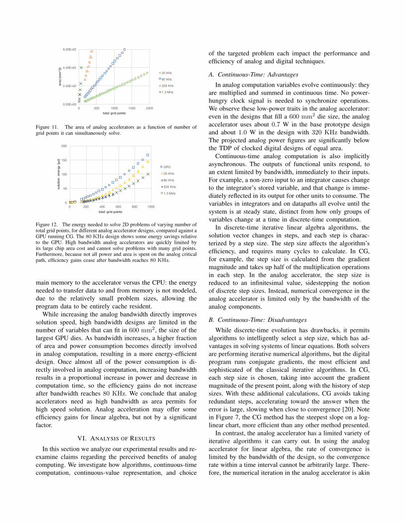
Figure 11. The area of analog accelerators as a function of number ofgrid points it can simultaneously solve.

0

50

100

150

200

0 200 400 600 800 1000

solu

tion

ener

gy (

J)

total grid points

GPU

20 KHz

80 KHz

320 KHz

1.3 MHz

Figure 12. The energy needed to solve 2D problems of varying number oftotal grid points, for different analog accelerator designs, compared against aGPU running CG. The 80 KHz design shows some energy savings relativeto the GPU. High bandwidth analog accelerators are quickly limited byits large chip area cost and cannot solve problems with many grid points.Furthermore, because not all power and area is spent on the analog criticalpath, efficiency gains cease after bandwidth reaches 80 KHz.

main memory to the accelerator versus the CPU: the energyneeded to transfer data to and from memory is not modeled,due to the relatively small problem sizes, allowing theprogram data to be entirely cache resident.

While increasing the analog bandwidth directly improvessolution speed, high bandwidth designs are limited in thenumber of variables that can fit in 600 mm2, the size of thelargest GPU dies. As bandwidth increases, a higher fractionof area and power consumption becomes directly involvedin analog computation, resulting in a more energy-efficientdesign. Once almost all of the power consumption is di-rectly involved in analog computation, increasing bandwidthresults in a proportional increase in power and decrease incomputation time, so the efficiency gains do not increaseafter bandwidth reaches 80 KHz. We conclude that analogaccelerators need as high bandwidth as area permits forhigh speed solution. Analog acceleration may offer someefficiency gains for linear algebra, but not by a significantfactor.

VI. ANALYSIS OF RESULTS

In this section we analyze our experimental results and re-examine claims regarding the perceived benefits of analogcomputing. We investigate how algorithms, continuous-timecomputation, continuous-value representation, and choice

of the targeted problem each impact the performance andefficiency of analog and digital techniques.

A. Continuous-Time: Advantages

In analog computation variables evolve continuously: theyare multiplied and summed in continuous time. No power-hungry clock signal is needed to synchronize operations.We observe these low-power traits in the analog accelerator:even in the designs that fill a 600 mm2 die size, the analogaccelerator uses about 0.7 W in the base prototype designand about 1.0 W in the design with 320 KHz bandwidth.The projected analog power figures are significantly belowthe TDP of clocked digital designs of equal area.

Continuous-time analog computation is also implicitlyasynchronous. The outputs of functional units respond, toan extent limited by bandwidth, immediately to their inputs.For example, a non-zero input to an integrator causes changeto the integrator’s stored variable, and that change is imme-diately reflected in its output for other units to consume. Thevariables in integrators and on datapaths all evolve until thesystem is at steady state, distinct from how only groups ofvariables change at a time in discrete-time computation.

In discrete-time iterative linear algebra algorithms, thesolution vector changes in steps, and each step is charac-terized by a step size. The step size affects the algorithm’sefficiency, and requires many cycles to calculate. In CG,for example, the step size is calculated from the gradientmagnitude and takes up half of the multiplication operationsin each step. In the analog accelerator, the step size isreduced to an infinitesimal value, sidestepping the notionof discrete step sizes. Instead, numerical convergence in theanalog accelerator is limited only by the bandwidth of theanalog components.

B. Continuous-Time: Disadvantages

While discrete-time evolution has drawbacks, it permitsalgorithms to intelligently select a step size, which has ad-vantages in solving systems of linear equations. Both solversare performing iterative numerical algorithms, but the digitalprogram runs conjugate gradients, the most efficient andsophisticated of the classical iterative algorithms. In CG,each step size is chosen, taking into account the gradientmagnitude of the present point, along with the history of stepsizes. With these additional calculations, CG avoids takingredundant steps, accelerating toward the answer when theerror is large, slowing when close to convergence [20]. Notein Figure 7, the CG method has the steepest slope on a log-linear chart, more efficient than any other method presented.

In contrast, the analog accelerator has a limited variety ofiterative algorithms it can carry out. In using the analogaccelerator for linear algebra, the rate of convergence islimited by the bandwidth of the design, so the convergencerate within a time interval cannot be arbitrarily large. There-fore, the numerical iteration in the analog accelerator is akin

to fixed-step size relaxation or steepest descent. While wecan consider the analog accelerator as doing continuous-time steepest descent, taking many infinitesimal steps incontinuous time, doing many iterations of a poor algorithmis in this case no match for a better algorithm. Efficientdiscrete-time algorithms such as CG, multigrid, and spectralmethods were known to researchers by the 1950s. Analogcomputers remained in use in the 1960s to solve steepestdescent due to their better immediate performance relativeto early digital computers.

C. Continuous-Value: Advantages

Changing the value of a digital binary number affectsmany bits. For example, sweeping an 8-bit unsigned integerfrom 0 to 255 needs 502 binary inversions. Using moreeconomical Gray coding, 255 inversions are still needed tosweep the range of an 8-bit integer. In general, the amountof charge needed for binary arithmetic is an exponentialfunction of precision. To worsen the case for digital, realvariables are usually encoded in floating point, which arecostlier per operation. The logarithmically encoded expo-nent portion of floating point variables makes adding andsubtracting variables complicated.

Analog computing is economical because real values areencoded in physical attributes, such as electrical current.The amount of energy needed to change the value of avariable is proportional to the size of the change in value.The precision of an analog variable is only limited by itssignal to noise ratio. In effect, a single wire can capture manybits of information. Finally, no special hardware is neededto sum and subtract analog values encoded as current. Theanalog crossbars can sum values by simply joining branches.

D. Continuous-Value: Disadvantages

Despite its efficiency, continuous-value representation inthe analog accelerator has drawbacks when used to assistdigital computing. While the computation taking place insidethe accelerator takes place at high precision, ADC conver-sion of the results is not so favorable. Each time the analogaccelerator runs to solve an equation, the digital host onlyobtains as many bits of precision as the ADC conversion.At the levels of ADC precision we consider, 8 − 12 bits,the digital algorithm takes only a few iterations to reach thesame level of precision. On the other hand, while operationon floating points is costly, the digital algorithm can continueoperating on the same set of data until precision is limitedby the precision of floating point numbers.

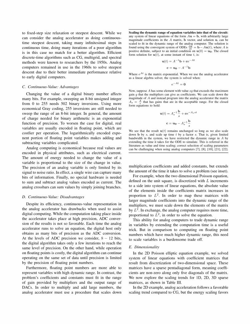
Furthermore, floating point numbers are more able torepresent variables with high dynamic range. In contrast, theproblem’s coefficients and constants must fit in the rangeof gain provided by multipliers and the output range ofDACs. In order to multiply and add large numbers, theanalog accelerator must use a procedure that scales down

Scaling the dynamic range of equation variables into that of the circuit:any system of linear equations of the form Au = b, with arbitrarily largemagnitude coefficients in the A matrix, b vector, and solution u, can bescaled to fit in the dynamic range of the analog computer. The solution isfound using the convergent system of ODEs du

dt= b−Au(t), where A is

positive definite, subject to an initial condition on u(0) = u0. The closedform solution for u(t), at some instant of time t, is:

u(t) = A−1b+ ce−At

c = u0 −A−1b

Where eAt is the matrix exponential. When we use the analog acceleratoras a linear algebra solver, the system is solved when:

e−At = 0

Now, suppose A has some element with value sg that exceeds the maximumgain g that the multipliers can give as coefficients. We can scale down themagnitude of A and instead program into the analog accelerator the matrixAs = A

sthat has gains that are in the acceptable range. For the closed

form equations to hold:

u(t) = A−1s

b

s+ ce−Asst

c = u0 −A−1s

b

s

We see that the result u(t) remains unchanged so long as we also scaledown b by s, and scale up time t by a factor s. That is, given limitedbandwidth in the system, we have restricted the dynamic range in A byextending the time it takes for the ODE to simulate. This is referred in theliterature as value and time scaling; correct selection of scaling parameterscan be challenging when using analog computers [7], [8], [10], [21], [22].

multiplication coefficients and added constants, but extendsthe amount of the time it takes to solve a problem (see inset).

For example, when the two dimensional Poisson equation,defined on the unit square, is discretized with L incrementsto a side into system of linear equations, the absolute valueof the elements inside the coefficients matrix increases inproportion to L2. In order to map these matrices withlarger magnitude coefficients into the dynamic range of themultipliers, we must scale down the elements of the matrixby L2. In exchange, the analog computer requires more time,proportional to L2, in order to solve the equation.

This ability for analog computers to trade dynamic rangein variables by extending the computation time is a usefultrick. But in comparison to computing on floating pointnumbers which have much higher dynamic range, this needto scale variables is a burdensome trade off.

E. Dimensionality

In the 2D Poisson elliptic equation example, we solvedsystem of linear equations with coefficient matrices thatresult from discretization of two-dimensional space. Thesematrices have a sparse pentadiagonal form, meaning coeffi-cients are non-zero along only five diagonals of the matrix.We now explore the scaling trends for 1D, 2D, 3D sparsematrices, as shown in Table III.

In the 2D example, analog acceleration follows a favorablescaling trend compared to CG, but the energy scaling favors

Analog Conjugate gradientsGrid points HW cost Conv. time Energy=HW×time Convergence steps Time per step Time and energy

1D N = L N = L integrators N = L N2 = L2 N = L N = L N2 = L2

2D N = L2 N = L2 integrators N = L2 N2 = L4 N0.5 = L N = L2 N1.5 = L3

3D N = L3 N = L3 integrators N = L3 N2 = L6 weak dependence N = L3 N = L3

Table IIITIME, AREA, AND ENERGY TRENDS FOR ANALOG ACCELERATION AND CONJUGATE GRADIENTS, FOR DIFFERENT TYPES OF CONNECTIVITY BETWEENVARIABLES, WHICH AFFECTS THE A MATRIX. N DENOTES THE NUMBER OF VARIABLES. L DENOTES THE NUMBER OF INCREMENTS PER DIMENSION.

CG. The overall effect there is a range of number of variablesbeing solved where analog possibly wins in both speed andenergy consumption.

In 3D problems, analog acceleration is not feasible, due tocomparable scaling of solution speed and unfavorable scal-ing of energy consumption. Changing the dimensionality ofthe problem from 2D to 3D poses no significant challengesto a software algorithm. For each node value, the stencil willrequest node values in neighbors in all three dimensions. Thenode values for neighbors in the highest order dimension willbe least recently used, and will have the least data locality.Compared to 2D problems, 3D problems have a larger datacache footprint, and an increase in the cache access stridelength.

Analog computing, on the other hand, faces greater chal-lenges in creating a hardware mapping for 3D problems ona 2D chip, due to difficulty in laying out the integrators in away that balances and minimizes the analog interconnects.

F. Targeted Problem Class

Efficient linear algebra algorithms form the heart ofmodern continuous math workloads. These linear algebraalgorithms operate on discrete-value variables which evolvein discrete time steps, which are approximations of the realdynamics of the physical world. Our objective was to applyanalog computing to sparse systems, a fundamental kernelfound in applications, with the hypothesis that a continuousmodel would yield benefits. Nonetheless, the intense demandfor efficient linear algebra has led to powerful digital algo-rithms, optimized to run well on digital hardware, that makediscrete approximations worthwhile, making the baseline inthis study difficult to beat.

The analog accelerator is fundamentally an ODE dynam-ics simulator, meaning useful computational results are in thedynamic output waveform. As discussed in Section II-B, thedynamic output waveform has uses in embedded systems,where analog computation results are directly useful indriving actuators. In this paper we consider analog accel-eration for digital computers, which potentially limits usefulcomputation results to the steady state output, which can beprecisely measured with slow, high-precision ADCs.

Analog acceleration may have greater benefits in otherdomains of continuous math, such as solving nonlinearPDEs. As shown in Figure 4, the solution of nonlinear PDEs

proceeds in the same way as in the linear case, typicallywith discretization into nonlinear ODEs, then using implicitsolvers that require solving systems of algebraic equations ateach time step. The key difference is these are now nonlinearsystems of equations, requiring Newton-Raphson method-based iterative solvers. These iterative solvers have contin-uous time formulations, which again involve solving ODEsof the form du

dt = f(u(t)). It is within our near future workto investigate how analog techniques can solve nonlinearproblems, which can be vexing for digital algorithms.

VII. RELATED WORK

Analog electronic computers were used in the 1950sand 1960s for scientific simulations, including problemsin optimization, ODEs, and PDEs [8]–[10], [21], [23]. By1968 attention shifted to hybrid analog-digital computers,which introduced digital computers to provide capaciousmemory and ability to do discrete-time algorithms [11]–[14]. In the years since, digital computers, which providedthe convenience and noise margin of binary variable encod-ing, capacious memory, and versatile numerical algorithms,eliminated analog computing from general use.

The development of analog and hybrid computers ranin parallel with the development of digital differentialanalyzers, which were digital numerical processors wherevariables were encoded in binary and evolved in discretetime. The digital units in DDAs were connected in thesame topology of an analog computer, according to thedifferential equation being solved [7]. These designs faceddifficulties in number dynamic range and scaling, which ledto the development of extended resolution and floating-pointvariants of DDAs [22], [24]. These area-intensive functionunits were used in a time-multiplexed fashion, previewingthe development of modern floating-point pipelines [25].

Computing using analog signals is resurgent in architec-ture research, due to challenges in IC scaling that limit thepower dissipated by digital circuits [26], [27]. Analog com-puting circuits can be instantiated alongside digital circuitsto handle workloads from a direct, numerical standpoint [1]–[5], [18], [28], [29], or to handle workloads developed in thefield of neuromorphic computing.

In neuromorphic computing, broad classes of applicationsusing both discrete and continuous variables are mapped toa variety of neural network topologies [30]–[32]. The neural

networks can in turn be simulated as software, or can be sim-ulated using resistive analog networks and A/D conversion,giving efficient multiplication and nonlinear lookups [33].In neuroscience, analog circuits have been investigated formodeling ODEs that describe non-trivial neurons.

We draw distinction between our approach to analogacceleration and that of neuromorphic computing. Mostimportant, we do not use training to get a network topologyand weights that solve a given problem. No prior knowledgeof the solution or training set of solutions is required. Theanalog acceleration technique presented here is a proceduralapproach to solving problems: there is a predefined way toconvert a system of linear equations under study into ananalog accelerator configuration.

Second, the analog computation presented in our workthrives on the possibility of connecting outputs of integratorsto their inputs. This is in contrast to most neuromorphiccomputing approaches, which use cellular neural networks,autoencoders, and multilayer perceptrons, which are purelyfeedforward networks. The full crossbar between analogcomponents allow any topology, including cycles, betweencomponents. In neural network terminology such topologiesare recurrent neural networks and Hopfield networks, andrepresent the most powerful class of networks.

Among other emerging architectures, the quantum algo-rithm for linear systems of equations allows characterizationof the solution vector in order of logN time, where N is thesize of the solution vector [34]. The solution is not readilymeasurable, but the algorithm has uses in algorithms thatrely on linear algebra [35].

VIII. CONCLUSIONS

In this work we discussed how analog computing is differ-ent from digital computing in these key aspects: the variablesevolve continuously in time; the variables have a continuousrange of values; and the algorithm executed on the hardwareis distinct. We presented an architecture for using solutionsgiven by an analog accelerator, and we discussed methodsto control downsides of analog computing such as limitedproblem size, limited dynamic range, and limited precision.

We used analog acceleration to solve systems of linearequations, an attractive and important application for thisnovel hardware design. Among linear algebra problems with2D connectivity, analog acceleration may have both 10×higher performance and 33% lower energy consumption,within a range of problem sizes. Notably, the obviousapproach to improving analog accelerator performance, byincreasing the analog circuit bandwidth, provides speedups,and can offer solutions requiring less energy, but has higharea costs.

We recognize the performance increases and energy sav-ings are not as drastic as one expects when using a fun-damentally different computing model than digital, syn-chronous computing. This is primarily due to highly efficient

algorithms for digital computers which are the dominantfactor in comparing solver systems, implemented as eitherdigital or analog hardware. Other numerical subroutines,such as those used in finding solutions to nonlinear systemsof equations, present greater challenges to existing algo-rithms, and may show promise for analog computing.

ACKNOWLEDGMENT

This work is supported by NSF award CNS-1239134 anda fellowship from the Alfred P. Sloan Foundation.

REFERENCES

[1] G. Cowan, R. Melville, and Y. Tsividis, “A VLSI analogcomputer/math co-processor for a digital computer,” in Solid-State Circuits Conference, 2005. Digest of Technical Papers.ISSCC. 2005 IEEE International, Feb 2005, pp. 82–586 Vol.1.

[2] ——, “A VLSI analog computer/digital computer accelera-tor,” Solid-State Circuits, IEEE Journal of, vol. 41, no. 1, pp.42–53, Jan 2006.

[3] N. Guo, Y. Huang, T. Mai, S. Patil, C. Cao, M. Seok,S. Sethumadhavan, and Y. Tsividis, “Continuous-time hybridcomputation with programmable nonlinearities,” in EuropeanSolid-State Circuits Conference (ESSCIRC), ESSCIRC 2015- 41st, Sept 2015, pp. 279–282.

[4] ——, “Energy-efficient hybrid analog/digital approximatecomputation in continuous time,” Solid-State Circuits, IEEEJournal of, vol. 51, Jul 2016, to be published.

[5] B. Schell and Y. Tsividis, “A clockless ADC/DSP/DACsystem with activity-dependent power dissipation and noaliasing,” in Solid-State Circuits Conference, 2008. ISSCC2008. Digest of Technical Papers. IEEE International, Feb2008, pp. 550–635.

[6] K. Asanovic, R. Bodik, B. C. Catanzaro, J. J. Gebis,P. Husbands, K. Keutzer, D. A. Patterson, W. L. Plishker,J. Shalf, S. W. Williams, and K. A. Yelick, “The landscapeof parallel computing research: A view from Berkeley,”EECS Department, University of California, Berkeley,Tech. Rep. UCB/EECS-2006-183, Dec 2006. [Online].Available: http://www.eecs.berkeley.edu/Pubs/TechRpts/2006/EECS-2006-183.html

[7] B. Ulmann, Analog Computing. Oldenbourg Wis-senschaftsverlag, 2013.

[8] W. Karplus and W. Soroka, Analog Methods: Computationand Simulation, ser. McGraw-Hill series in engineering sci-ences. McGraw-Hill, 1959.

[9] A. Jackson, Analog computation. McGraw-Hill, 1960.

[10] S. Fifer, Analogue Computation: Theory, Techniques, and Ap-plications, ser. Analogue Computation: Theory, Techniques,and Applications. McGraw-Hill, 1961, no. v. 3.

[11] G. Bekey and W. Karplus, Hybrid computation. Wiley, 1968.

[12] W. Chen and L. P. McNamee, “Iterative solution of large-scale systems by hybrid techniques,” IEEE Transactions onComputers, vol. C-19, no. 10, pp. 879–889, Oct 1970.

[13] W. J. Karplus and R. Russell, “Increasing digital computerefficiency with the aid of error-correcting analog subroutines,”Computers, IEEE Transactions on, vol. C-20, no. 8, pp. 831–837, Aug 1971.

[14] G. Korn and T. Korn, Electronic analog and hybrid comput-ers. McGraw-Hill, 1972.

[15] C. C. Douglas, J. Mandel, and W. L. Miranker, “Fast hybridsolution of algebraic systems,” SIAM Journal on Scientificand Statistical Computing, vol. 11, no. 6, pp. 1073–1086,1990. [Online]. Available: http://dx.doi.org/10.1137/0911060

[16] Y. Zhang, “Revisit the analog computer and gradient-basedneural system for matrix inversion,” in Intelligent Control,2005. Proceedings of the 2005 IEEE International Symposiumon, Mediterranean Conference on Control and Automation,June 2005, pp. 1411–1416.

[17] Y. Zhang and S. S. Ge, “Design and analysis of a generalrecurrent neural network model for time-varying matrix in-version,” Neural Networks, IEEE Transactions on, vol. 16,no. 6, pp. 1477–1490, Nov 2005.

[18] S. Sethumadhavan, R. Roberts, and Y. Tsividis, “A casefor hybrid discrete-continuous architectures,” IEEE Comput.Archit. Lett., vol. 11, no. 1, pp. 1–4, Jan. 2012. [Online].Available: http://dx.doi.org/10.1109/L-CA.2011.22

[19] S. Keckler, W. Dally, B. Khailany, M. Garland, and D. Glasco,“GPUs and the future of parallel computing,” Micro, IEEE,vol. 31, no. 5, pp. 7–17, Sept 2011.

[20] J. R. Shewchuk, “An introduction to the conjugate gradientmethod without the agonizing pain,” 1994.

[21] B. Wilkins, Analogue and iterative methods in computation,simulation, and control, ser. Modern electrical studies. Chap-man and Hall, 1970.

[22] R. B. McGhee and R. N. Nilsen, “The extended resolutiondigital differential analyzer: A new computing structure forsolving differential equations,” IEEE Transactions on Com-puters, vol. C-19, no. 1, pp. 1–9, Jan 1970.

[23] W. Karplus, Analog simulation: solution of field problems, ser.McGraw-Hill series in information processing and computers.McGraw-Hill, 1958.

[24] J. L. Elshoff and P. T. Hulina, “The binary floatingpoint digital differential analyzer,” in Proceedings of theNovember 17-19, 1970, Fall Joint Computer Conference,ser. AFIPS ’70 (Fall). New York, NY, USA: ACM, 1970,pp. 369–376. [Online]. Available: http://doi.acm.org/10.1145/1478462.1478516

[25] G. Hannington and D. G. Whitehead, “A floating-point multi-plexed DDA system,” IEEE Transactions on Computers, vol.C-25, no. 11, pp. 1074–1077, Nov 1976.

[26] H. Esmaeilzadeh, E. Blem, R. St. Amant, K. Sankaralingam,and D. Burger, “Dark silicon and the end of multicorescaling,” in Proceedings of the 38th Annual InternationalSymposium on Computer Architecture, ser. ISCA ’11. NewYork, NY, USA: ACM, 2011, pp. 365–376. [Online].Available: http://doi.acm.org/10.1145/2000064.2000108

[27] M. B. Taylor, “Is dark silicon useful? harnessing the fourhorsemen of the coming dark silicon apocalypse,” in DesignAutomation Conference, 2012.

[28] E. H. Lee and S. S. Wong, “A 2.5GHz 7.7TOPS/W switched-capacitor matrix multiplier with co-designed local memoryin 40nm,” in 2016 IEEE International Solid-State CircuitsConference (ISSCC), Jan 2016, pp. 418–419.

[29] S. George, S. Kim, S. Shah, J. Hasler, M. Collins, F. Adil,R. Wunderlich, S. Nease, and S. Ramakrishnan, “A pro-grammable and configurable mixed-mode FPAA SoC,” IEEETransactions on Very Large Scale Integration (VLSI) Systems,vol. PP, no. 99, pp. 1–9, 2016.

[30] T. Chen, Y. Chen, M. Duranton, Q. Guo, A. Hashmi,M. Lipasti, A. Nere, S. Qiu, M. Sebag, and O. Temam,“BenchNN: On the broad potential application scope ofhardware neural network accelerators,” in Proceedingsof the 2012 IEEE International Symposium on WorkloadCharacterization (IISWC), ser. IISWC ’12. Washington, DC,USA: IEEE Computer Society, 2012, pp. 36–45. [Online].Available: http://dx.doi.org/10.1109/IISWC.2012.6402898

[31] S. Esser, A. Andreopoulos, R. Appuswamy, P. Datta,D. Barch, A. Amir, J. Arthur, A. Cassidy, M. Flickner,P. Merolla, S. Chandra, N. Basilico, S. Carpin, T. Zimmer-man, F. Zee, R. Alvarez-Icaza, J. Kusnitz, T. Wong, W. Risk,E. McQuinn, T. Nayak, R. Singh, and D. Modha, “Cognitivecomputing systems: Algorithms and applications for networksof neurosynaptic cores,” in Neural Networks (IJCNN), The2013 International Joint Conference on, Aug 2013, pp. 1–10.

[32] Y. Chen, T. Luo, S. Liu, S. Zhang, L. He, J. Wang, L. Li,T. Chen, Z. Xu, N. Sun, and O. Temam, “DaDianNao: Amachine-learning supercomputer,” in Microarchitecture (MI-CRO), 2014 47th Annual IEEE/ACM International Sympo-sium on, Dec 2014, pp. 609–622.

[33] R. St. Amant, A. Yazdanbakhsh, J. Park, B. Thwaites,H. Esmaeilzadeh, A. Hassibi, L. Ceze, and D. Burger,“General-purpose code acceleration with limited-precisionanalog computation,” SIGARCH Comput. Archit. News,vol. 42, no. 3, pp. 505–516, Jun. 2014. [Online]. Available:http://doi.acm.org/10.1145/2678373.2665746

[34] A. W. Harrow, A. Hassidim, and S. Lloyd, “Quantumalgorithm for linear systems of equations,” Phys. Rev.Lett., vol. 103, p. 150502, Oct 2009. [Online]. Available:http://link.aps.org/doi/10.1103/PhysRevLett.103.150502

[35] S. Aaronson, “Read the fine print,” Nature Physics, vol. 11,no. 4, pp. 291–293, 2015.