Transportation Consortium of South-Central States

Solving Emerging Transportation Resiliency, Sustainability, and Economic Challenges through the Use of Innovative Materials and Construction Methods: From Research to Implementation

Evaluation of Comparative Damaging Effects of Multiple Truck Axles for Flexible Pavements Project No. 17PUTA02

Lead University: University of Texas at Arlington

Collaborative Universities: University of Texas at San Antonio

Final Report

December 2018

Enhancing Durability and Service Life of Infrastructure

i

Disclaimer The contents of this report reflect the views of the authors, who are responsible for the facts and the accuracy of the information presented herein. This document is disseminated in the interest of information exchange. The report is funded, partially or entirely, by a grant from the U.S. Department of Transportation’s University Transportation Centers Program. However, the U.S. Government assumes no liability for the contents or use thereof.

Acknowledgments The authors would like to acknowledge the financial support for this study by the Transportation Consortium of South-Central States (Tran-SET) and the support with field testing and material sampling provided by Justin Thomey and Ngozi Lopez with the Texas Department of Transportation (TxDOT), Fort Worth District, and by Hector Hernandez with Rodriguez Engineering Laboratories LLC.

ii

TECHNICAL DOCUMENTATION PAGE 1. Project No. 17PUTA01

2. Government Accession No.

3. Recipient’s Catalog No.

4. Title and Subtitle 5. Report Date Dec. 2018

Evaluation of Comparative Damaging Effects of Multiple Truck Axles for Flexible Pavements

6. Performing Organization Code

7. Author(s) PI: Stefan A. Romanoschi https://orcid.org/0000-0002-3051-3320 Co-PI: Athanasios Papagiannakis https://orcid.org/0000-0002-3047-7112

8. Performing Organization Report No.

9. Performing Organization Name and Address Transportation Consortium of South-Central States (Tran-SET)

10. Work Unit No. (TRAIS)

Transportation Consortium of South-Central States (Tran-SET) University Transportation Center for Region 6 3319 Patrick F. Taylor Hall, Louisiana State University, Baton Rouge, LA 70803

11. Contract or Grant No. 69A3551747106

12. Sponsoring Agency Name and Address United States of America Department of Transportation

13. Type of Report and Period Covered Final Research Report Jun. 2017 – Nov. 2018

Research and Innovative Technology Administration 14. Sponsoring Agency Code

15. Supplementary Notes Report uploaded and accessible at: Tran-SET's website (http://transet.lsu.edu/) 16. Abstract This study aims at evaluating the effect of overlapping flexible pavement strain responses from truck axles that are not part of multiple axle configurations (i.e., tandem, triple and quad). For this purpose, a newly constructed pavement was instrumented with strain gauges installed at the bottom of the asphalt concrete base layer on US-287 south of Mansfield, TX. This pavement structure is typically used for medium- to high-volume roads in the South-Central region of the United States. The strain gauges were used to measure longitudinal and transverse strains under several passes of a test vehicle. This was a class 6 truck with a steering axle load of 56.9 kN (12.8 kips) and a tandem drive axle load of 161.9 kN (36.4 kips). The speed and the lateral position of the vehicle were recorded for each test vehicle pass. Sufficient quantities of the top two layers of asphalt concrete were obtained during construction to allow dynamic modulus testing in the laboratory. The general-purpose finite element program Abaqus was used to model the instrumented pavement section and compute the longitudinal and transverse strains at the location of the strain gauges. In the analysis, the asphalt concrete layers were modeled as visco-elastic materials. The Abaqus estimated strains were found in good agreement with the measured strains. Both the field measurements and the finite element analysis showed that the strains under the passing of the steering axle were of similar magnitude as the strains under the passing of the rear tandem axle. The measured transverse strains were in general slightly larger than the corresponding longitudinal strains. This can be attributed to the accumulation of strain from the front axle and the rear axle that takes place only in the transverse direction. However, the finite element model computed higher strains in the longitudinal direction than in the transverse direction. These findings suggest the need to account for the overlap in strain responses from the steering and the following axles of trucks. Furthermore, findings suggest that both the longitudinal and the transverse strain responses need to be considered in evaluating the fatigue damage impacted from trucks.

17. Key Words Strain signals; Flexible pavement response; Truck axle effect

18. Distribution Statement No restrictions.

19. Security Classif. (of this report) Unclassified

20. Security Classif. (of this page) Unclassified

21. No. of Pages 74

22. Price

Form DOT F 1700.7 (8-72) Reproduction of completed page authorized.

iii

SI* (MODERN METRIC) CONVERSION FACTORS APPROXIMATE CONVERSIONS TO SI UNITS

Symbol When You Know Multiply By To Find Symbol LENGTH

in inches 25.4 millimeters mm ft feet 0.305 meters m yd yards 0.914 meters m mi miles 1.61 kilometers km

AREA in2 square inches 645.2 square millimeters mm2

ft2 square feet 0.093 square meters m2

yd2 square yard 0.836 square meters m2

ac acres 0.405 hectares ha mi2 square miles 2.59 square kilometers km2

VOLUME fl oz fluid ounces 29.57 milliliters mL gal gallons 3.785 liters L ft3 cubic feet 0.028 cubic meters m3

yd3 cubic yards 0.765 cubic meters m3

NOTE: volumes greater than 1000 L shall be shown in m3

MASS oz ounces 28.35 grams glb pounds 0.454 kilograms kgT short tons (2000 lb) 0.907 megagrams (or "metric ton") Mg (or "t")

TEMPERATURE (exact degrees) oF Fahrenheit 5 (F-32)/9 Celsius oC

or (F-32)/1.8 ILLUMINATION

fc foot-candles 10.76 lux lx fl foot-Lamberts 3.426 candela/m2 cd/m2

FORCE and PRESSURE or STRESS lbf poundforce 4.45 newtons N lbf/in2 poundforce per square inch 6.89 kilopascals kPa

APPROXIMATE CONVERSIONS FROM SI UNITS Symbol When You Know Multiply By To Find Symbol

LENGTHmm millimeters 0.039 inches in m meters 3.28 feet ft m meters 1.09 yards yd km kilometers 0.621 miles mi

AREA mm2 square millimeters 0.0016 square inches in2

m2 square meters 10.764 square feet ft2

m2 square meters 1.195 square yards yd2

ha hectares 2.47 acres ac km2 square kilometers 0.386 square miles mi2

VOLUME mL milliliters 0.034 fluid ounces fl oz L liters 0.264 gallons gal m3 cubic meters 35.314 cubic feet ft3

m3 cubic meters 1.307 cubic yards yd3

MASS g grams 0.035 ounces ozkg kilograms 2.202 pounds lbMg (or "t") megagrams (or "metric ton") 1.103 short tons (2000 lb) T

TEMPERATURE (exact degrees) oC Celsius 1.8C+32 Fahrenheit oF

ILLUMINATION lx lux 0.0929 foot-candles fc cd/m2 candela/m2 0.2919 foot-Lamberts fl

FORCE and PRESSURE or STRESS N newtons 0.225 poundforce lbf kPa kilopascals 0.145 poundforce per square inch lbf/in2

iv

TABLE OF CONTENTS LIST OF FIGURES ................................................................................................................ VI

LIST OF TABLES ................................................................................................................ VIII

ACRONYMS, ABBREVIATIONS, AND SYMBOLS ......................................................... IX

EXECUTIVE SUMMARY ...................................................................................................... X

IMPLEMENTATION STATEMENT .................................................................................... XI

1. INTRODUCTION .................................................................................................................1

1.1 Asphalt Concrete Fatigue Damage Models ............................................................ 1

1.2 Pavement Modeling and Instrumentation ............................................................... 3

1.2.1 Instrumentation at the MnROAD Test Site ............................................. 4

1.2.2 Instrumentation at Virginia Tech’s Smart Road ...................................... 5

1.2.3 Instrumentation at NCAT’s Test Track ................................................... 6

1.2.4 Kansas Perpetual Pavement Test Site ...................................................... 8

1.2.5 University of Waterloo CPATT Test Site ................................................ 8

1.3 Heavy Truck Impact on Fatigue Damage ............................................................. 10

2. OBJECTIVE ........................................................................................................................12

3. SCOPE .................................................................................................................................13

4. METHODOLOGY ..............................................................................................................14

4.1. Field Test Site ...................................................................................................... 14

4.1.1. Location of Test Site ............................................................................. 14

4.1.2. Hot Mix Asphalt ................................................................................... 16

4.2. Stiffness Properties of HMA Mixes ..................................................................... 19

4.2.1. Dynamic Resilient Modulus Testing .................................................... 19

4.2.2. Comparison of E* measured with the E* Predicted by the Witczak Model .................................................................................................. 27

4.3. Instrumentation Installation and Measuring Procedure ...................................... 29

4.3.1. Response Monitoring Instrumentation .................................................. 29

4.3.2. Response Measuring Procedure ........................................................... 31

v

4.4. The Finite Element Simulation of the Passing of the Test Vehicle ..................... 34

4.4.1. Model Geometry ................................................................................... 34

4.4.2. Material Characterization ...................................................................... 36

4.4.3. Element Type and Size ......................................................................... 39

4.4.4. Boundary Conditions ............................................................................ 41

4.4.5. Loading ................................................................................................. 42

5. FINDINGS ...........................................................................................................................45

5.1. Response Data Analysis ....................................................................................... 45

5.2. Results of the Finite Element Analysis ................................................................ 50

5.3. Comparison of Measured and Computed Strains ................................................ 53

6. CONCLUSIONS..................................................................................................................57

7. RECOMMENDATIONS .....................................................................................................58

REFERENCES ........................................................................................................................59

APPENDIX A: MEASURED STRAIN SIGNALS ................................................................61

vi

LIST OF FIGURES Figure 1. Transverse strain signal from MnROAD test (5). ..................................................... 5

Figure 2. Transverse strain measurements at VA Tech’s Smart Road (8)................................ 6

Figure 3. Longitudinal strains measurements at VA Tech’s Smart Road (8). .......................... 6

Figure 4. NCAT strain gauge installation (8). .......................................................................... 7

Figure 5. Example of longitudinal strain measurement from NCAT site (8). .......................... 8

Figure 6. Pavement instrumentation by KSU (10).................................................................... 9

Figure 7. Longitudinal and transverse strain measurements at the KSU Site (10). .................. 9

Figure 8. Strain gauge installation at the U. of Waterloo (11). ............................................... 10

Figure 9. Longitudinal strain measurements at U. of Waterloo’s CPATT Test Site (11). ..... 10

Figure 10. Example of cycle counting in fatigue analysis (14). ............................................. 11

Figure 11. Project location. ..................................................................................................... 14

Figure 12. The Intersection of US-360 and US-287. .............................................................. 15

Figure 13. Aerial view of the Intersection of US-360 and US-287. ....................................... 15

Figure 14. Aggregate gradation chart for Mix S. .................................................................... 18

Figure 15. Aggregate gradation chart for Mix I. ..................................................................... 18

Figure 16. Aggregate gradation chart for Mixes B. ................................................................ 19

Figure 17. Sample obtained from superpave gyratory compactor. ......................................... 20

Figure 18. Configuration of the dynamic resilient modulus test. ........................................... 21

Figure 19. Typical output at 10 Hz. ........................................................................................ 22

Figure 20. Typical Output at 0.1 Hz. ...................................................................................... 22

Figure 21. Average dynamic modulus for Mix S. .................................................................. 26

Figure 22. Average dynamic modulus for Mix I. ................................................................... 26

Figure 23. Average Dynamic Modulus for Mix B. ................................................................. 27

Figure 24. Plan view of the instrumentation. .......................................................................... 29

Figure 25. Schematic of strain gauges Model KM-100-HAS................................................. 30

Figure 26. Coring and groove cut in the HMA base layer. ..................................................... 31

Figure 27. Strain gauge glued to the HMA Core. ................................................................... 31

Figure 29. Schematic of a truck passing over an instrumented pavement section. ................ 35

vii

Figure 30. Geometry of the finite element model. .................................................................. 35

Figure 31. Dynamic modulus master curve for Mix S............................................................ 36

Figure 32. Dynamic modulus master curve for Mix I. ........................................................... 37

Figure 33. Dynamic modulus master curve for Mix B. .......................................................... 37

Figure 34. Element type and size. ........................................................................................... 40

Figure 35. The elements used (a) C3D8R Finite and (b) CIN3D8 Infinite. ........................... 41

Figure 36. Boundary conditions of the model. ....................................................................... 41

Figure 37. Tire imprint dimensions. ....................................................................................... 42

Figure 38. Wheel path surface partition. ................................................................................. 43

Figure 39. Schematic of a moving tire based on the trapezoidal loading method. ................. 44

Figure 40. Example strain signal. ........................................................................................... 45

Figure 41. Measured strains under the steering wheel. ........................................................... 49

Figure 42. Measured strains under the first rear wheel. .......................................................... 49

Figure 43. Measured strains under the second rear wheel. ..................................................... 50

Figure 44. Computed strain signals at the bottom of HMA layer. .......................................... 53

Figure 45. Measured versus estimated strains under the steering wheel. ............................... 55

Figure 46. Measured versus estimated strains under the first rear wheel. .............................. 55

Figure 47. Measured versus estimated strains under the second rear wheel. ......................... 56

viii

LIST OF TABLES Table 1. The configuration of the pavement structure. ........................................................... 16

Table 2. HMA mix characteristics. ......................................................................................... 17

Table 3. Gradation analysis..................................................................................................... 17

Table 4. Mix volumetric properties. ....................................................................................... 17

Table 5. Dynamic modulus (MPa) for Mix S at different frequencies. .................................. 23

Table 6. Phase angle (degrees) for Mix S at different frequencies. ........................................ 23

Table 7. Dynamic modulus (MPa) for Mix I at different frequencies. ................................... 24

Table 8. Phase angle (degrees) for Mix I at different frequencies. ......................................... 24

Table 9. Dynamic modulus (MPa) for Mix B at different frequencies. .................................. 25

Table 10. Phase angle (degrees) for Mix B at different frequencies. ..................................... 25

Table 11. Recommended values of A and VTS based on binder grade (3). ........................... 28

Table 12. Measured and predicted dynamic moduli (MPa). ................................................... 28

Table 13. Tire dimensions and weight of the test truck. ......................................................... 32

Table 14. Speed and transverse position of the vehicle during strain measurements. ............ 33

Table 15. Temperatures recorded during strain measurements. ............................................. 33

Table 16. Structural layers used in the finite element geometry model. ................................. 35

Table 17. Layers moduli used in the FE model analysis. ....................................................... 38

Table 18. Prony series parameters. ......................................................................................... 39

Table 19. Wheel load transition parameters. .......................................................................... 43

Table 20. Loading amplitude tabular data for 50 mph. ........................................................... 44

Table 21. Measured transverse strain values. ......................................................................... 47

Table 22. Measured longitudinal strain values. ...................................................................... 48

Table 23. Subdivided Loading Amplitude Tabular Data for 50 mph. .................................... 51

Table 24. Transverse strains computed by the FE model. ...................................................... 52

Table 25. Longitudinal strains computed by the FE Model.................................................... 54

ix

ACRONYMS, ABBREVIATIONS, AND SYMBOLS AASHTO American Association of State Highway and Transportation Officials

CELB Civil Engineering Laboratory

DOT Department of Transportation

FE Finite Element

FHWA Federal Highway Administration

HMA Hot Mix Asphalt

KSU Kansas State University

NCHRP National Cooperative Highway Research Program

SGC Superpave Gyratory Compactor

TXDOT Texas Department of Transportation

UTM Universal Testing Machine

x

EXECUTIVE SUMMARY In order to estimate the damage caused by heavy vehicles on flexible pavement structures, a newly constructed pavement was instrumented with strain gauges retrofitted at the bottom of an asphalt concrete pavement base layer. The instrumented section is located on highway US-287, to the South of Mansfield, TX and it represents a flexible pavement structure typically used for medium- and high-volume roads in the South-Central region of the United States. The strain gauges were used to measure longitudinal and transverse strains under several passes of a test vehicle having a steering axle with single tires and a rear tandem axle with dual tires. The speed and the lateral position of the vehicle were recorded for each pass. Sufficient quantities of the top two layers of asphalt concrete were obtained during construction to manufacture cores in the laboratory and obtain their dynamic modulus. The general-purpose finite element program Abaqus was used to model this instrumented pavement section and to compute the longitudinal and transverse strains. In the analysis, the asphalt concrete layers were modeled as visco-elastic materials with the parameters derived from the results of the dynamic modulus tests.

The field experiments and the finite element analysis showed that the strains under the passing of the steering axle were of similar magnitude as the strains under the passing of each of the rear drive axles. The measured transverse strains were mostly slightly higher than the corresponding longitudinal strains. This can be attributed to the accumulation of strain from the front axle and the rear axle that takes place only in the transverse direction. However, the finite element model computed higher strains in the longitudinal direction than in the transverse direction. The measured and computed strains were always lower than 25 microstrain, which is significantly lower than 70 microstrain considered as the endurance limit for hot mix asphalt.

This research study recommends the inclusion of the damage induced by steering axles and the computation of the transverse strains in addition to that of longitudinal strains for the estimation of fatigue damage at the bottom of the asphalt layers. The measured and computed strains were always lower than 25 microstrain, lower than 70 microstrain considered as the endurance limit for hot mix asphalt. Therefore, it is recommended that the use of a thick asphalt concrete layer and a lime-stabilized subgrade soil layer as a mean of prolonging pavement fatigue life.

xi

IMPLEMENTATION STATEMENT The results of this research project will be disseminated to the pavement design groups within the State Departments of Transportation (DOTs) in Region 6. The dissemination will focus on state level agencies since only state DOTs are implementing Mechanistic-Empirical (M-E) design methods (e.g., AASHTOWare Pavement ME, TxME) for flexible pavement structures. Once state DOTs complete the implementation of the findings of this research study, it is expected that other local agencies will follow their lead and will use the improved M-E design methods.

Furthermore, an educational module on pavement response measurements and on theoretical computation of stresses and strains and truck damage will be developed and implemented in the Pavement Design course at the University of Texas at Arlington and the University of Texas at San Antonio. Finally, the knowledge acquired in this investigation will be shared at national and international conferences such as the TRB Annual Meeting, the 2019 Tran-SET Conference, the annual AAPT conference, and the World Transport Convention (WTC).

1

1. INTRODUCTION Heavy vehicle axle loads induce pavement strains that drive pavement damage accumulation which untimely leads to pavement distress. Fatigue cracking is one of the dominant pavement distress mechanisms in flexible pavements. Traditional fatigue cracking in asphalt pavements is governed by the tensile strains, longitudinal and transverse, at the bottom of the asphalt concrete layer. These strains generate tension fatigue cracks that originate at the bottom and propagate to the top of the asphalt concrete layer. Multiple axle configurations, such as tandems and triples, generate strain responses that overlap; that is the strain from the lead axle does not quite recover before the strain from the following axle begins to build up. This results in multi-hump strain responses under closely-spaced adjacent truck axles. Accounting for the damaging effect of these multiple strain cycles is essential in evaluating the damaging effects of multiple truck axle configurations. While this issue has been thoroughly researched, it remains unclear whether pavement strains from unconnected axles could overlap as well, under certain circumstances. For example, is there an overlap between the strains from steering axles and those from the following tandem drive axles of a Class 9 semi-trailer truck? Some studies suggest that for thick asphalt concrete layers and high vehicle speeds this may be possible. If so, the way pavement fatigue damage from heavy trucks needs to be reevaluated to account for the effect of strain overlap from successive truck axles.

The objective of this study is to develop a strain measurement dataset that will allow revisiting pavement strain response under in-service traffic for the purpose of quantifying pavement damage under consecutive axle load configurations. In addition, the pavement layer properties from the instrumented pavement site will allow comparing the measured versus estimated strains using conventional layer visco-elastic analysis techniques.

A literature search was undertaken to gather detailed information on previous and on-going studies dealing with flexible pavement response predictions and measurements under multiple truck axles, and their effect on pavement fatigue damage. The Transportation Research Information Database (TRID) database was used for this purpose. The literature search focused on:

• Asphalt concrete fatigue cracking damage models, • Pavement instrumentation focusing on asphalt concrete strain measurements, and • Evaluation of the impact of various truck configurations considering the effect of

overlapping strain cycles from consecutive axles groups.

1.1 Asphalt Concrete Fatigue Damage Models Pavement fatigue damage that results in bottom-up fatigue cracking failure has been associated with tensile strain since the early 1960s. Experimental work by Finn (1) established that the relationship between tensile strain and the number of cycles to fatigue failure Nf is highly non-linear (Equation 1).

𝑁𝑁𝑖𝑖 = 𝑘𝑘1(1𝜀𝜀

)𝑘𝑘2 [1]

2

Subsequent fatigue damage work recognized the importance of the modulus E of the asphalt concrete layer in pavement damage accumulation. The following damage relationship was adopted by the mechanistic design approach developed by the Asphalt Institute (2):

𝑁𝑁𝑓𝑓 = 0.007566 (1𝜀𝜀𝑡𝑡

)3.9492 (1𝐸𝐸

)1.281 [2]

A modified version of this relationship was adopted for the Mechanistic-Empirical Pavement Design Guide (ME-PDG) (3) to account for the thickness of the asphalt concrete layer and the volumetric properties of the mix:

𝑁𝑁𝑓𝑓 = 0.007566 𝛽𝛽𝑓𝑓1𝐶𝐶𝐻𝐻𝐶𝐶(1𝜀𝜀𝑡𝑡

)3.9492 𝛽𝛽𝑓𝑓2(1𝐸𝐸

)1.281 𝛽𝛽𝑓𝑓3 [3]

where: 𝜀𝜀𝑡𝑡 = the tensile strain in the asphalt concrete layer, E = its dynamic modulus (lbs/in2), and 𝛽𝛽𝑓𝑓1, 𝛽𝛽𝑓𝑓2, and 𝛽𝛽𝑓𝑓3 = calibration constants with default values of 1.0.

The coefficient C is a volumetric correction and CH is a thickness correction. C is given by:

𝐶𝐶 = 10𝑀𝑀 [4]

with:

𝑀𝑀 = 4.84(𝑉𝑉𝑏𝑏𝑏𝑏

𝑉𝑉𝑎𝑎 + 𝑉𝑉𝑏𝑏𝑏𝑏) − 0.69 [5]

where: Vbe = the effective volume of binder, and Va = the volume of the mix as a percentage of the total mix volume.

The correction CH is a function of the thickness of the asphalt concrete layer hac (inches). For conventional bottom-up fatigue cracking is given by:

𝐶𝐶𝐻𝐻 =1

0.000398 + 0.0036021 + 𝑒𝑒11.02−3.49ℎ𝑎𝑎𝑎𝑎

[6]

Fatigue damage FD (percent) is accumulated according to Miner’s hypothesis (4) expressed as:

𝐹𝐹𝐹𝐹 = 𝛴𝛴𝑛𝑛𝑖𝑖,𝑗𝑗,𝑘𝑘,𝑙𝑙,𝑚𝑚

𝑁𝑁𝑖𝑖,𝑗𝑗,𝑘𝑘,𝑙𝑙,𝑚𝑚100 [7]

where: ni,j,k,… = applied number of load applications at condition i, j, k, l, m, n, Ni,j,k,… = number of axle load applications to cracking failure under conditions i, j, k, l, m,

3

i = month, which accounts for monthly changes in the moduli of base and subgrade due to moisture variations and asphalt concrete due to temperature variations, j = time of the day, which accounts for hourly changes in the modulus of the asphalt concrete, k = axle type, (i.e., single, tandem, triple and quad), l = load level for each axle type, and m = traffic path, assuming a normally distributed lateral wheel wander.

The bottom-up fatigue cracking area FCbottom (i.e., alligator cracking in % of total lane area) is computed as:

𝐹𝐹𝐶𝐶𝑏𝑏𝑏𝑏𝑡𝑡𝑡𝑡𝑏𝑏𝑚𝑚 =1

60𝐶𝐶4

1 + 𝑒𝑒(𝐶𝐶1𝐶𝐶1∗+𝐶𝐶2𝐶𝐶2∗ log(𝐹𝐹𝐹𝐹𝑏𝑏𝑏𝑏𝑏𝑏𝑏𝑏𝑏𝑏𝑏𝑏100)) [8]

where: 𝐹𝐹𝐹𝐹𝑏𝑏𝑏𝑏𝑡𝑡𝑡𝑡𝑏𝑏𝑚𝑚 = the bottom-up fatigue damage (percent) computed from Equations 6 and 7, and 𝐶𝐶1, 𝐶𝐶2, and 𝐶𝐶4 are transfer function regression constants with values of 1.0, 1.0 and 6000, respectively.

The remaining coefficients are as follows:

𝐶𝐶1∗ = −2𝐶𝐶2∗ [9]

𝐶𝐶2∗ = −2.40874 − 39.748(1 + ℎ𝑎𝑎𝑎𝑎)−2.856 [10]

Typically, the criterion used for bottom-up fatigue failure is defined as 50% of the wheel area cracked.

In summary, flexible pavement fatigue damage and the associated cracking depend on traffic-induced strains, as well as the dynamic modulus of the asphalt concrete layer, its thickness and volumetric properties. Hence, Equation 3 can be used to estimate the fatigue damage accumulated from successive truck axles, by adding the damage resulting from the magnitude of the tensile strain cycles generated by individual axles. Furthermore, Equations 7 suggests that 1 load cycle generating a tensile strain of magnitude 𝜀𝜀𝑡𝑡 causes fatigue damage amounting to 1/Nf. These are the two basic equations that will be used in evaluating the damaging effect of multiple truck axles of various configurations.

1.2 Pavement Modeling and Instrumentation The technology for obtaining in-situ measurements of pavement response has grown from the need to validate layer elastic analysis techniques which evolved along with digital computing. There is a multitude of layer elastic analysis continuum models and software including:

• The Waterways Experimental Station’s WESLEA, • Shell’s BISAR, • ELSYM5 developed for the Federal Highway Administration (FHWA), • Huang’s KENLAYER, and • Uzan’s JULEA, which was incorporated into the M-E PDG software.

4

Their common features include, axial symmetry (i.e., two-dimensional displacement field), circular tire imprints, homogeneous and isotropic linear elastic layer properties and bottom layer of infinite depth. In addition, there is a variety of finite element (FE) models, both 2-D and 3-D that can handle the analysis of more complex layered systems including viscoelastic layer properties, non-linear (i.e., stress-dependent) granular layer properties, actual tread-shaped contact stresses and moving dynamic loads. Commercial software packages, such as Abaqus and ANSYS, have been used extensively for this purpose. In addition, a number of custom pavement analysis FE models have been developed, such as MICHPAV and CAPA3D.

Pavement instrumentation has evolved with the need to verify pavement response prediction models, such as the ones outlined above. Amongst the earlier efforts in pavement instrumentation were in the 1960s and 1970s. More recent pavement instrumentation installations include pavement test road sites, such as MnROAD, Virginia Tech's Smart Road, NCAT’s instrumented pavement site and U. Waterloo’s CPATT site. In addition to test track installations, pavement instrumentation has been used extensively under accelerated pavement loading through various Accelerated Pavement Test (APT) facilities. Examples abound:

• FHWA’s Heavy Vehicle Simulator, • California’s Accelerated Pavement Testing Facility, • U. of Illinois’s Advanced Transportation Loading Assembly (ATLAS), • Louisiana State University’s Accelerated Load Facility, • Ohio’s Accelerated Pavement Testing Facility, • CREEL’s Heavy Vehicle Simulator, and • Florida DOT’s Accelerated Pavement Testing facility.

The following sections focus on instrumentation installations on major test roads, as they are most relevant to the study at hand.

1.2.1 Instrumentation at the MnROAD Test Site The MnROAD test site (5, 6) that involved a multitude of strain gauges, pressure cells, LVDT deflection transducers, as well as temperature and moisture gauges. Strain gauges were installed parallel and perpendicular to the direction of travel, approximately 1 inch above the bottom of the AC layer. Two types of strain gauges were installed, namely H-shaped Dynatest PAST-II gauges embedded in a strip of glass-fibre reinforced epoxy, and Tokyo-Sokki PML-60 gauges consisting of a single folded wire hermetically sealed in a resin casing. One of the main applications of the MnROAD strain measurement data was to develop mechanistic Load Equivalence Factors (LEFs) in terms of pavement fatigue damage. Several fatigue damage relationships were used for this purpose. The factorial experiment involved a multitude of axle configurations, speeds, tire inflation pressures and pavement temperatures. An example of the transverse strain readings caused by the passage of a 5-axle semitrailer is shown in Figure 1. It is evident that the strain between the drive and trailer axles does not fully recover (i.e., return to zero) and as a result there is overlap in the strain responses of these two axles.

5

Figure 1. Transverse strain signal from MnROAD test (5).

1.2.2 Instrumentation at Virginia Tech’s Smart Road The Virginia Tech’s Smart Road incorporated 12 heavily instrumented pavement sections that were equipped with Dynatest Past-IIAC and Kyowa KM-120 strain gauges, as well as pressure cells and environmental monitoring sensors (7). Both gauge types were H-shaped, but the Dynatest gauges were proven more reliable than those made by Kyowa. These strain gauges were installed both longitudinally and transversely at the bottom of the asphalt concrete layer of each test section. The survivability of these strain gauges was about 95% immediately after construction and about 75% 5 years later. In addition, vibrating wire strain gauges were installed at the bottom of the granular base layer for measuring static tensile strain. Loading involved a 6-axle semi-trailer truck (i.e., steering and tandem in the tractor and tridem axle in the trailer). Examples of transverse and longitudinal strain measurements under this truck are shown in Figures 2 and 3. The significant drop in strain measurements under the tridem axle was explained by axle off-tracking. These figures suggest transverse strains, rather than longitudinal strains, not recovering between the steering and tandem tractor axles.

6

Figure 1. Transverse strain measurements at VA Tech’s Smart Road (8).

Figure 3. Longitudinal strains measurements at VA Tech’s Smart Road (8).

1.2.3 Instrumentation at NCAT’s Test Track The NCAT instrumented pavement site utilised a multitude of sensors, strain gauges, pressure cells of different sizes, subgrade compression gauges as well as temperature and moisture (i.e., time-domain reflectometry) gauges (8). The strain gauges used were manufactured by Construction Technologies Laboratory (CTL). These are H-shaped with an active gauge length of 2 inches. The strain gauges, both longitudinal and transverse were installed 3 side-to-side along three alignments, one at the edge of the outer wheel path and the two others 2 feet on either side of the edge of the outer wheel path (Figure 4). Both longitudinal and transverse strain gauges were installed at the Sets of these gauges were installed at the bottom of the

7

asphalt concrete layer that is at depths of 5 or 7 inches depending on the layer thickness at the test location. The advantages of this arrangement were reported as redundancy (i.e., same gauge installation on the same alignment provides measurement replication) as well as indirect estimation of axle lateral placement (i.e., the higher the strains at a particular station, the closer the tires are to this location). Lateral vehicle placement was established using a vertical-facing digital video camera and reflective tape on the pavement.

• An example of longitudinal strain measurements under a triple trailer truck are shown in Figure 5. In this case, no residual strain seems to exit between successive axle groups. Some of the findings from the NCAT instrumented site most relevant to the study at hand are:

• The variability between strain gauges under the same axle load is likely due to vehicle wander.

• Longitudinal gauges exhibited lower variability than transverse gauges, likely due to their lower vehicle wander sensitivity.

• Pavement cracking affected strain measurements. The 80th percentile of crack-free sections generated absolute variation between strain gauges lower than 30 με.

• The 90th percentile of crack-free sections generate absolute variation within strain gauges lower than 6 με.

Figure 4. NCAT strain gauge installation (8).

8

Figure 2. Example of longitudinal strain measurement from NCAT site (8).

1.2.4 Kansas Perpetual Pavement Test Site Kansas State University (KSU) has developed an instrumented pavement site to study perpetual pavements. A layout of the instrumentation installation is shown in Figure 6. The strain gauges and pressure cells were arranged along two alignments, 36 inches and 30 inches from the edge of the driving lane. The strain gauges were H-shaped Tokyo-Sokki and were arranged longitudinally and transversely to the direction of travel at the bottom of a 10-inch thick asphalt concrete layer (10). An example of the strain measurements obtained is shown in Figure 7. As seen by the blue line, there is no full recovery of the longitudinal strain generated by the steering axle of the Class 8 vehicle before strains begin to build up from its tandem drive axles.

1.2.5 University of Waterloo CPATT Test Site An instrumented pavement site was developed in the vicinity of the U. of Waterloo Campus in Ontario Canada (11). It is equipped with a multitude of pavement sensors (i.e., asphalt concrete strain gauges base layer load cells and environmental sensors) as well as deep-seated sensors for measuring embankment displacement and strain (Figure 8). The asphalt concrete strain gauges were installed at the bottom of layers 10 inches and 7 inches thick. An example of the longitudinal strains measured in the 10-inch asphalt concrete layer at 15 mph is shown in Figure 9. This is another example of the steering axle strain axle not fully recovering before the onset of the drive axle strain cycle.

9

Figure 3. Pavement instrumentation by KSU (10).

Figure 4. Longitudinal and transverse strain measurements at the KSU Site (10).

10

Figure 8. Strain gauge installation at the U. of Waterloo (11).

Figure 9. Longitudinal strain measurements at U. of Waterloo’s CPATT Test Site (11).

1.3 Heavy Truck Impact on Fatigue Damage Fatigue damage accumulation from complex strain histories follows the rain-flow counting technique described by ASTM Standard 1049-85(2017) (13). This technique is explained through Figure 10. The complex strain history shown in Figure 9, is split into complete sub-cycles, such for example the first cycle from A to B and from B to the same level of strain as A along the path B, the second cycle from E to F and from F to the same level as E along the FG path, and so on for the remaining cycles. The technique resembles the filling with water of the strain history turned upside down, which give this technique its name. The magnitude

11

of the strain cycles established in this fashion gives defines the damage accumulated by this complex strain history. For these 4 cycles and given Miner’s hypothesis (Equation 7), the damage F accumulated is given by:

𝐹𝐹 =1𝑁𝑁𝑓𝑓1

+1𝑁𝑁𝑓𝑓2

+1𝑁𝑁𝑓𝑓3

+1𝑁𝑁𝑓𝑓4

[11]

where: 𝑁𝑁𝑓𝑓𝑖𝑖 = the number of cycles to fatigue failure from strain cycle i.

For flexible pavement fatigue analysis, the number of cycles to failure is given by Equation 3 described earlier. A study by Papagiannakis et al. (14) gives an example of applying this technique in estimating mechanistic load equivalence factors for flexible pavement pavements.

Figure 10. Example of cycle counting in fatigue analysis (14).

12

2. OBJECTIVE The objective of this project is to develop a strain measurement dataset that will allow revisiting pavement response under in-service traffic for the purpose of comparing longitudinal and transverse strains under the front and rear axle of heavy vehicles. An additional objective is to compare the measured strains with the strains estimated using conventional layer visco-elastic techniques. The outcome of the project will help the south-central state DOTs and local agency officials make more informed decisions about the effect of truck axle loads and configurations on pavement response and damage. It will allow a proper estimation of pavement structural response, which will lead to improved flexible pavement design. It will also help with the refinement of the AASHTOWare Pavement ME and TxME software.

13

3. SCOPE The scope of this project is to develop a strain measurement dataset and compare longitudinal and transverse strains under the front and rear axle of heavy vehicles for pavement structures with thick asphalt pavement built on top of thick layers of lime-treated embankment clay soils. This structural configuration is used vastly by state DOTs and local agencies for medium to heavy truck traffic corridors in Region 6. In the region, clay soils are the most common and lime-treated embankment layers are an extensively used solution for addressing the variability of subgrade soil properties along road construction projects, reducing the permanent deformation under truck traffic and reducing the potential for volume change in the subgrade soil layer.

14

4. METHODOLOGY 4.1. Field Test Site 4.1.1. Location of Test Site The field site for installing the instrumentation was selected amongst the new paving projects Texas Department of Transportation (TxDOT) had in the 2018 season. The test site was on a construction project on highway US-287, south of Mansfield, TX, in Johnson County, right at the intersection with US-360. The location where the sensors were installed is in the North-West bound outside lane, immediately before the overpass over US-360. The location is indicated in the maps shown in Figures 11 to 13; the maps were obtained from Google Earth.

This construction project was selected since it was a new flexible pavement construction with a relatively thick asphalt concrete layer and carries medium to high truck traffic volume. The instrumentation was installed with assistance from the construction company and the client (TxDOT) while the road was being constructed.

Figure 11. Project location.

15

Figure 12. The Intersection of US-360 and US-287.

Figure 13. Aerial view of the Intersection of US-360 and US-287.

The road section in the location where the sensors were installed was built over two years. The contractor finalized the earthwork in November 2016. The geotechnical investigation

16

identified the natural sub-grade soils along the project as a high plasticity clay. The embankment on all four pavement sections was brought to grade and the top thirty-six inches of soil were stabilized with 6% by weight hydrated lime in August 2017 to ensure proper support to the asphalt concrete layers and to provide a stable support for the construction equipment. Appropriate measures were taken for the proper curing of the lime treated soil. The configuration of the pavement structure is given in Table 1.

Table 1. The configuration of the pavement structure.

Layer Description Wearing Course 1.5 inches, Mix S (SMA; PG70-28) Binder Course 2.5 inches, Mix I (TxDOT Type D; PG64-22) Base Course 6.5 inches, Mix B (TxDOT Type B; PG 64-22) Chemically Stabilized Embankment Soil

36.0 inches, 6% hydrated lime mixed to the natural soil

Natural Sub-grade High plasticity clay (A-7-6) High plasticity clay (A-7-7)

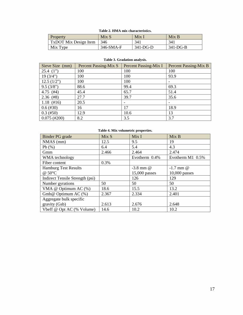
4.1.2. Hot Mix Asphalt The asphalt paving work was done from November 2017 to June 2018. The project was completed and the experimental sections were opened to traffic in July 2018. As shown in Table 1, three different HMA mixes were used in the construction of the pavement section. The mix characteristics of all three mixes are given in Table 2. The aggregate gradation data and volumetric properties, as well as binder grade are provided in Tables 3 and 4 while the gradation curves are shown in Figures 14 to 16. The mixes were designed following TxDOT’s mix design methods specified for Item 341 (dense graded mixes) and Item 346 (SMA) (15).

Mix B was used only for the base layer. The layer was paved to a thickness of eight inches in Fall 2017 and it was milled down to a thickness of 6.5 inches in Spring 2018. Mixes S and I were used in the construction of the wearing and intermediate courses, respectively. Mixes B and I are typical for the mixes used on state roads in the North Texas region. Mix S was a Stone Matrix Asphalt (SMA), a mix type used only on few construction projects in the region.

Sufficient quantities of hot mix were obtained from the asphalt plant for mixes S and I. The materials were transported to the Civil Engineering Laboratory (CELB) of the University of Texas at Arlington (UTA) where cylindrical specimens, 6 inch in diameter and 7 inch in height, were manufactured using the Superpave Gyratory Compactor. The specimens, compacted at the target air void content of 7.0% were cored and trimmed to obtain cylindrical samples 4 inch in diameter and 6 inch in height. The samples were tested to determine the dynamic modulus of the two mixes.

17

Table 2. HMA mix characteristics.

Property Mix S Mix I Mix B TxDOT Mix Design Item 346 341 341 Mix Type 346-SMA-F 341-DG-D 341-DG-B

Table 3. Gradation analysis.

Sieve Size (mm) Percent Passing-Mix S Percent Passing-Mix I Percent Passing-Mix B 25.4 (1”) 100 100 100 19 (3/4") 100 100 93.9 12.5 (1/2") 100 100 - 9.5 (3/8") 88.6 99.4 69.3 4.75 (#4) 45.4 65.7 51.4 2.36 (#8) 27.7 39.7 35.6 1.18 (#16) 20.5 - - 0.6 (#30) 16 17 18.9 0.3 (#50) 12.9 10.6 13 0.075 (#200) 8.2 3.5 3.7

Table 4. Mix volumetric properties.

Binder PG grade Mix S Mix I Mix B NMAS (mm) 12.5 9.5 19 Pb (%) 6.4 5.4 4.3 Gmm 2.466 2.464 2.474 WMA technology Evotherm 0.4% Evotherm M1 0.5% Fiber content 0.3% Hamburg Test Results @ 50°C

-3.8 mm @ 15,000 passes

-1.7 mm @ 10,000 passes

Indirect Tensile Strength (psi) 126 129 Number gyrations 50 50 50 VMA @ Optimum AC (%) 18.6 15.5 13.2 Gmb@ Optimum AC (%) 2.367 2.334 2.401 Aggregate bulk specific gravity (Gsb) 2.613 2.676 2.648 Vbeff @ Opt AC (% Volume) 14.6 10.2 10.2

18

Figure 14. Aggregate gradation chart for Mix S.

Figure 15. Aggregate gradation chart for Mix I.

19.0

12.59.5

4.75

2.36

1.18

0.600.30

0.07

50.

15

0

10

20

30

40

50

60

70

80

90

100

Perc

ent P

assi

ng

(%)

Sieve size (mm)

25.4

19.0

12.5

9.5

4.75

2.36

1.18

0.60

0.15

0.30

0.07

50

10

20

30

40

50

60

70

80

90

100

Perc

ent P

assi

ng

(%)

Sieve size (mm)

19

Figure 16. Aggregate gradation chart for Mixes B.

4.2. Stiffness Properties of HMA Mixes 4.2.1. Dynamic Resilient Modulus Testing The dynamic resilient modulus testing is a cyclic compressive test performed on cylindrical asphalt specimens with the dimensions of 100 mm diameter (4 in) and 150 mm height (6 in). The test was performed according to “Simple Performance Test for Permanent Deformation Based upon Dynamic Modulus of Asphalt Concrete Mixtures” (16).

In this test a sinusoidal axial compressive load is applied to the cylindrical specimen at a sweep of loading frequencies. During testing, the UTM system measures the vertical stress and the resulting vertical compression strain. The dynamic resilient modulus is calculated by dividing the peak to peak vertical compressive stress to the peak-to-peak vertical strain.

The cylinders were cored from samples with 150 mm diameter (6 in.) fabricated in the Superpave Gyratory Compactor (Figure 17) and sawed at the ends, at the Civil Engineering Laboratory (CELB) of UT Arlington. The samples were made from hot mix obtained during the construction of the surface (Mix S) and intermediate (Mix I) layers. No hot mix could be obtained from the base layer (Mix B) since this layer was placed prior to the commencement of this research. The compacted samples need to be cored and sawed on the plane surfaces in order to obtain a cylinder with a smooth surface, free from ridges or grooves. The air void content was determined for each sample after the testing.

Three LVDTs were mounted on the side of the specimen using a system of screws and nuts glued with epoxy to the specimen (Figure 18). The axial deformation of the central region of the specimen is computed by averaging the deformation recorded by the three LVDTs. The

19.0

12.59.5

4.75

2.36

1.180.60

0.15 0.30

0.07

5

25.4

0

10

20

30

40

50

60

70

80

90

100

Perc

ent P

assi

ng

(%)

Sieve size (mm)

20

distance between the centerline of the glued screws was 100 mm and was considered as the gauge length.

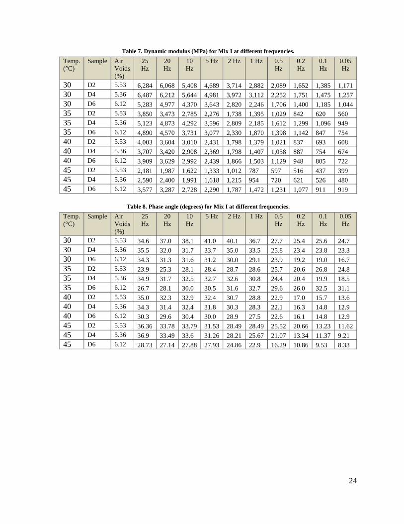
The asphalt specimens were tested at four temperatures 30oC, 35oC, 40oC, and 45oC and ten load frequencies (25 Hz, 20 Hz, 10 Hz, 5 Hz, 2 Hz, 1 Hz, 0.5 Hz, 0.2 Hz, 0.1 Hz, and 0.05 Hz). The specimens were conditioned in the environmental chamber for at least two hours before testing. In this testing configuration, each specimen is placed centered on the steel plate. The LVDTs are fixed to the glued nuts and, the top steel plate is centered on the specimen to ensure centric loading. The actuator is gradually lowered until it touches slightly the top plate.

Once the preparation and mounting of the asphalt cylinder specimen is finished the test is controlled entirely by the CDAS. The cyclic load is applied by the actuator through the steel plate placed on the top of the specimen. The cycling loading is applied at a succession of ten load frequencies in the following order: 25 Hz (100 cycles), 20 Hz (50 cycles), 10 Hz (50 cycles), 5 Hz (50 cycles), 2 Hz (50 cycles), 1 Hz (30 cycles), 0.5 Hz (7 cycles), 0.2 Hz (7 cycles), 0.1 Hz (5 cycles) and 0.05 Hz (5 cycles).

The following data were recorded periodically during the test: dynamic load and stress, microstrain, dynamic modulus, maximum and minimum load displacement, temperature, duration of test, phase angle. The data for each test were saved in a binary file format and ASCII text files. The text files were then imported into Microsoft Excel for further numerical analysis.

Figure 17. Sample obtained from Superpave Gyratory Compactor (SGC).

21

Figure 18. Configuration of the dynamic resilient modulus test.

Figures 19 and 20 show the typical stress-strain relationship recorded at 10 Hz and 0.1 Hz. It can be observed that absolute value of the total compressive strain is increasing with time, indicating an accumulation of plastic deformation during the cyclic compression test. The dynamic resilient modulus E* is calculated by dividing the peak-to-peak stress to the recoverable strain under a repeated sinusoidal waveform loading. For each load cycle, the final value is averaged and the dynamic resilient modulus is computed for each load frequency as:

𝐸𝐸∗ =𝑆𝑆0𝑒𝑒0

[12]

where: 𝐸𝐸∗= dynamic resilient modulus (MPa), 𝑆𝑆0 = applied stress amplitude (kN), and 𝑒𝑒0= strain amplitude.

The recoverable strain 𝑒𝑒0 is calculated as follows:

𝑒𝑒0 =𝑑𝑑𝐺𝐺𝐺𝐺

[13]

where: 𝑑𝑑 = average deformation amplitude (mm), and 𝐺𝐺𝐺𝐺 = gauge length, 100 mm for all samples.

22

Figure 19. Typical output at 10 Hz.

Figure 20. Typical Output at 0.1 Hz.

The results of the dynamic modulus test are given in Tables 5 to 10, along with the air void content of each sample tested. As expected, the dynamic modulus decreased with temperature and increased with loading frequency. The few exceptions that were observed for this trend may be because of the variability in aggregate structure, compaction levels and measurement errors.

Figures 21 to 23 show the variation of the average dynamic modulus with the temperature and the loading frequency for the two mixes tested. The values obtained for mixes S and I, slightly lower for mix S, which had a higher design binder content (6.4% vs 5.4%) and a stiffer binder (PG 76-22 vs PG 64-22) and a higher NMAS (12.5 mm vs 9.5mm) than mix I.

-60

-55

-50

-45

-40

0

60

120

180

240

0 0.1 0.2 0.3 0.4 0.5 0.6

Stra

in (

mic

ro-s

trai

n)

Stre

ss

(kPa

)

Time (sec.)

Stress Strain

-300

-200

-100

0

0

100

200

300

0 10 20 30 40 50 60

Stra

in (

mic

ro-s

trai

n)

Stre

ss

(kPa

)

Time (sec.)

Stress Strain

23

Table 5. Dynamic modulus (MPa) for Mix S at different frequencies.

Temp. (°C)

Sample Air Voids (%)

25 Hz

20 Hz

10 Hz

5 Hz 2 Hz 1 Hz 0.5 Hz

0.2 Hz

0.1 Hz

0.05 Hz

30 SMA2 5.77 5,709 5,421 4,742 4,015 3,207 2,559 1,902 1,549 1,337 1,160 30 SMA3 5.14 6,095 5,696 5,103 4,477 3,597 2,909 2,117 1,720 1,455 1,252 30 SMA4 5.23 7,032 6,698 5,719 5,120 3,998 3,137 2,292 1,801 1,523 1,285 35 SMA2 5.77 4,264 3,964 3,457 2,907 2,316 1,853 1,354 1,141 983 879 35 SMA3 5.14 4,500 4,253 3,732 3,124 2,502 1,996 1,427 1,180 999 887 35 SMA4 5.23 3,900 3,586 2,949 2,410 1,870 1,514 1,151 947 709 641 40 SMA2 5.77 3,146 2,966 2,450 2,040 1,609 1,304 968 832 715 652 40 SMA3 5.14 3,803 3,570 3,044 2,558 2,031 1,614 1,167 1,007 859 784 40 SMA4 5.23 3,373 3,125 2,557 2,131 1,628 1,313 1,006 862 725 668 45 SMA2 5.77 2,486 2,289 1,880 1,587 1,239 1,016 777 695 619 590 45 SMA3 5.14 2,722 2,532 2,107 1,817 1,437 1,183 901 821 735 707 45 SMA4 5.23 2,665 2,478 2,003 1,625 1,312 1,069 808 704 626 586

Table 6. Phase angle (degrees) for Mix S at different frequencies.

Temp. (°C)

Sample Air Voids (%)

25 Hz

20 Hz

10 Hz

5 Hz 2 Hz 1 Hz 0.5 Hz

0.2 Hz

0.1 Hz

0.05 Hz

30 SMA2 5.77 32.1 30.8 31.1 31.7 32.0 30.9 26.2 22.2 22.8 21.1 30 SMA3 5.14 28.7 29.7 30.6 33.3 34.2 34.2 28.8 25.3 26.6 25.9 30 SMA4 5.23 13.0 12.6 25.2 34.3 46.7 45.3 40.3 29.2 29.3 26.9 35 SMA2 5.77 32.7 32.2 33.2 33.0 32.4 30.8 26.2 20.2 19.6 17.6 35 SMA3 5.14 35.1 33.9 34.1 34.3 34.2 32.9 28.4 23.2 23.9 22.3 35 SMA4 5.23 25.8 26.9 29.6 28.8 28.3 28.8 28.3 20.7 27.4 24.7 40 SMA2 5.77 31.5 31.7 31.2 30.4 29.2 27.8 23.8 17.2 16.7 14.6 40 SMA3 5.14 33.7 31.1 31.8 31.6 29.8 28.2 23.3 17.8 17.2 15.5 40 SMA4 5.23 35.8 34.4 34.2 33.1 31.4 29.9 25.6 18.5 18.4 16.2 45 SMA2 5.77 30.71 34.24 35.79 34.1 31.93 29.79 25.9 18.43 18.21 16.29 45 SMA3 5.14 33.38 33.4 32.69 30.92 29.21 27.24 22.49 16.38 16.18 14.41 45 SMA4 5.23 28.29 32.94 33.59 31.42 29.49 27.66 23.45 16.26 16.41 14.6

24

Table 7. Dynamic modulus (MPa) for Mix I at different frequencies.

Temp. (°C)

Sample Air Voids (%)

25 Hz

20 Hz

10 Hz

5 Hz 2 Hz 1 Hz 0.5 Hz

0.2 Hz

0.1 Hz

0.05 Hz

30 D2 5.53 6,284 6,068 5,408 4,689 3,714 2,882 2,089 1,652 1,385 1,171 30 D4 5.36 6,487 6,212 5,644 4,981 3,972 3,112 2,252 1,751 1,475 1,257 30 D6 6.12 5,283 4,977 4,370 3,643 2,820 2,246 1,706 1,400 1,185 1,044 35 D2 5.53 3,850 3,473 2,785 2,276 1,738 1,395 1,029 842 620 560 35 D4 5.36 5,123 4,873 4,292 3,596 2,809 2,185 1,612 1,299 1,096 949 35 D6 6.12 4,890 4,570 3,731 3,077 2,330 1,870 1,398 1,142 847 754 40 D2 5.53 4,003 3,604 3,010 2,431 1,798 1,379 1,021 837 693 608 40 D4 5.36 3,707 3,420 2,908 2,369 1,798 1,407 1,058 887 754 674 40 D6 6.12 3,909 3,629 2,992 2,439 1,866 1,503 1,129 948 805 722 45 D2 5.53 2,181 1,987 1,622 1,333 1,012 787 597 516 437 399 45 D4 5.36 2,590 2,400 1,991 1,618 1,215 954 720 621 526 480 45 D6 6.12 3,577 3,287 2,728 2,290 1,787 1,472 1,231 1,077 911 919

Table 8. Phase angle (degrees) for Mix I at different frequencies.

Temp. (°C)

Sample Air Voids (%)

25 Hz

20 Hz

10 Hz

5 Hz 2 Hz 1 Hz 0.5 Hz

0.2 Hz

0.1 Hz

0.05 Hz

30 D2 5.53 34.6 37.0 38.1 41.0 40.1 36.7 27.7 25.4 25.6 24.7 30 D4 5.36 35.5 32.0 31.7 33.7 35.0 33.5 25.8 23.4 23.8 23.3 30 D6 6.12 34.3 31.3 31.6 31.2 30.0 29.1 23.9 19.2 19.0 16.7 35 D2 5.53 23.9 25.3 28.1 28.4 28.7 28.6 25.7 20.6 26.8 24.8 35 D4 5.36 34.9 31.7 32.5 32.7 32.6 30.8 24.4 20.4 19.9 18.5 35 D6 6.12 26.7 28.1 30.0 30.5 31.6 32.7 29.6 26.0 32.5 31.1 40 D2 5.53 35.0 32.3 32.9 32.4 30.7 28.8 22.9 17.0 15.7 13.6 40 D4 5.36 34.3 31.4 32.4 31.8 30.3 28.3 22.1 16.3 14.8 12.9 40 D6 6.12 30.3 29.6 30.4 30.0 28.9 27.5 22.6 16.1 14.8 12.9 45 D2 5.53 36.36 33.78 33.79 31.53 28.49 28.49 25.52 20.66 13.23 11.62 45 D4 5.36 36.9 33.49 33.6 31.26 28.21 25.67 21.07 13.34 11.37 9.21 45 D6 6.12 28.73 27.14 27.88 27.93 24.86 22.9 16.29 10.86 9.53 8.33

25

Table 9. Dynamic modulus (MPa) for Mix B at different frequencies.

Temp. (°C)

Sample Air Voids (%)

25 Hz

20 Hz

10 Hz

5 Hz 2 Hz 1 Hz 0.5 Hz

0.2 Hz

0.1 Hz

0.05 Hz

30 B1 5.08 4080 3769 3225 2919 2490 2105 1565 1355 1007 919 30 B2 7.03 4435 4120 3542 3139 2681 2288 1692 1484 1114 1042 30 B3 5.09 4946 4506 3894 3478 2968 2565 2034 1829 1491 1417 35 B1 5.08 3857 3537 3070 2685 2201 1778 1327 1150 978 877 35 B2 7.03 3796 3580 3165 2774 2309 1919 1430 1260 1083 995 35 B3 5.09 4490 4136 3632 3196 2641 2180 1711 1494 1317 1211 40 B1 5.08 3459 3149 2687 2286 1839 1494 1127 991 843 776 40 B2 7.03 3575 3261 2750 2383 1930 1596 1210 1065 913 849 40 B3 5.09 3365 3133 2670 2332 1902 1583 1238 1102 968 902 45 B1 5.08 3361 3051 2511 2123 1669 1347 1026 895 760 695 45 B2 7.03 2961 2659 2210 1875 1490 1224 934 830 715 665 45 B3 5.09 3134 2873 2359 1977 1569 1283 1027 930 822 781

Table 10. Phase angle (degrees) for Mix B at different frequencies.

Temp. (°C)

Sample Air Voids (%)

25 Hz

20 Hz

10 Hz

5 Hz 2 Hz 1 Hz 0.5 Hz

0.2 Hz

0.1 Hz

0.05 Hz

30 B1 5.08 19.22 20.48 22.87 22.98 23.85 25.10 21.88 20.23 28.60 27.86 30 B2 7.03 21.14 22.36 24.78 24.55 24.96 25.57 22.77 19.67 27.35 25.46 30 B3 5.09 20.04 21.26 22.66 22.94 23.74 24.71 21.92 18.90 26.76 26.71 35 B1 5.08 28.17 26.38 26.5 26.33 25.73 24.95 19.47 16.12 16.08 14.66 35 B2 7.03 28.6 26.37 27.13 26.4 25.89 25.18 20.06 16.04 15.95 14.43 35 B3 5.09 25.15 23.28 24.04 23.76 23.94 23.47 17.4 14.68 14.86 13.55 40 B1 5.08 27.37 26.22 26.7 25.7 24.91 24.32 19.3 14.77 13.99 12.4 40 B2 7.03 26.59 25.88 26.18 25.41 24 23.63 18.12 13.44 12.91 11.06 40 B3 5.09 25.28 24.31 25.2 24.74 23.93 23.55 18.56 13.45 12.86 10.63 45 B1 5.08 27.08 27.53 26.76 26.02 24.95 24.13 18.06 13.68 13.02 11.09 45 B2 7.03 25.3 24.5 24.86 23.85 22.07 21.75 19.94 11.99 11.35 9.4 45 B1 5.08 19.22 20.48 22.87 22.98 23.85 25.10 21.88 20.23 28.60 27.86

26

Figure 21. Average dynamic modulus for Mix S.

Figure 22. Average dynamic modulus for Mix I.

0

1,000

2,000

3,000

4,000

5,000

6,000

7,000

0.01 0.1 1 10 100

Dyn

amic

Mod

ulus

, E*

(M

Pa)

Frequency (Hz)

Average Dynamic Modulus - Mix S 30°C35°C40°C45°C

0

1,000

2,000

3,000

4,000

5,000

6,000

7,000

0.01 0.1 1 10 100

Dyn

amic

Mod

ulus

, E*

(M

Pa)

Frequency (Hz)

Average Dynamic Modulus - Mix I30°C35°C40°C45°C

27

Figure 23. Average Dynamic Modulus for Mix B.

4.2.2. Comparison of E* measured with the E* Predicted by the Witczak Model It is useful to compare the dynamic moduli values measured in the laboratory with the corresponding moduli predicted by the Witczak equation. This way, the differences in air void content and testing temperature are accounted for in the comparison. The Witczak equation for prediction of dynamic modulus is expressed as:

log|𝐸𝐸∗| = −1.249937 + 0.029232𝑃𝑃200 − 0.001767(𝑃𝑃200)2 + 0.002841𝑃𝑃4 − 0.058097𝑉𝑉𝑎𝑎

−0.802208𝑉𝑉𝑏𝑏𝑏𝑏𝑓𝑓𝑓𝑓

(𝑉𝑉𝑏𝑏𝑏𝑏𝑓𝑓𝑓𝑓 + 𝑉𝑉𝑎𝑎) +[3.871977 − 0.0021𝑃𝑃4 + 0.003958𝑃𝑃3

8− 0.000017(𝑃𝑃3

8)2 + 0.00547𝑃𝑃3

4]

1 + 𝑒𝑒(−0.603313−0.31335 log 𝑓𝑓−0.393532 log 𝑛𝑛)

[14]

where: 𝐸𝐸∗= asphalt mix dynamic modulus, in 105 psi, 𝑛𝑛 = bitumen viscosity in 106 poise (at any temperature, degree of aging), 𝑓𝑓 =load frequency in Hz, 𝑉𝑉𝑎𝑎 = air voids in the mix, % by volume, 𝑉𝑉𝑏𝑏𝑏𝑏𝑓𝑓𝑓𝑓 =effective bitumen content, % by volume, 𝑃𝑃3/4, 𝑃𝑃3/8, 𝑃𝑃4 , 𝑃𝑃200 = retained on the ¾ inch, 3/8 inch, No. 4, and No. 200 sieves, respectively, by total aggregate weight (%cumulative).

The bitumen viscosity is calculated using the following equation:

log log(𝜂𝜂) = 𝐴𝐴 + 𝑉𝑉𝑉𝑉𝑆𝑆 log𝑉𝑉𝑅𝑅 [15]

0500

1,0001,5002,0002,5003,0003,5004,0004,5005,000

0.01 0.1 1 10 100

Dyn

amic

Mod

ulus

, E*

(M

Pa)

Frequency (Hz)

Average Dynamic Modulus - Mix B30°C35°C40°C45°C

28

where: 𝜂𝜂 = viscosity, cP, VTS and A = regression slope and intercept of viscosity temperature susceptibility, and 𝑉𝑉𝑅𝑅= temperature, Rankine.

The A and VTS parameters can be estimated from the DSR test, penetration test or can be directly taken from the recommended values in the design guide. From the DSR test, the asphalt stiffness data at each temperature is converted to viscosity using the following equation:

𝜂𝜂 =𝐺𝐺∗

10(

1sin 𝛿𝛿

)4.8628 [16]

where: 𝜂𝜂 = viscosity, centipoises, 𝐺𝐺∗= complex shear modulus, Pa, and 𝛿𝛿 = phase angle, degrees.

The default values of A and VTS are given in the Table 11.

Table 11. Recommended values of A and VTS based on binder grade (3).

Binder PG Grade A VTS PG 64-22 10.980 -3.680 PG 76-22 9.715 -3.208

Table 12 presents the average measued and the corresponding predicted values for the dynamic modulus with the Witczak model, and their corresponding ratios. Average of reported air void content was used in the Witczak equation to predict the dynamic modulus. As shown in Table 12, the ratio of measured versus predicted dynamic moduli is between 0.378 and 0.551. This indicates that the Witczak model over-predicts the moduli of the two mixes for the studied temperatures and loading frequencies.

Table 12. Measured and predicted dynamic moduli (MPa).

Mechanism T (°C)

Mix S 25 Hz

Mix S 10 Hz

Mix I 25 Hz

Mix I 10 Hz

Mix B 25 Hz

Mix B 10 Hz

Measured 30 6,279 5,188 6,018 5,141 4,487 3,553 Measured 35 4,221 3,379 4,621 3,603 4,048 3,288 Measured 40 3,441 2,684 3,873 2,970 3,466 2,702 Measured 45 2,624 1,997 2,783 2,114 3,152 2,359 Predicted by Witczak Model 30 11,388 9,586 13,288 11,422 15,942 13,355 Predicted by Witczak Model 35 8,765 7,236 10,732 9,061 12,180 10,000 Predicted by Witczak Model 40 6,701 5,435 8,595 7,135 9,240 7,450 Predicted by Witczak Model 45 5,110 4,080 6,846 5,595 6,992 5,547 Measured / Predicted ratio 30 0.551 0.541 0.453 0.450 0.28 0.27 Measured / Predicted ratio 35 0.482 0.467 0.431 0.398 0.33 0.33 Measured / Predicted ratio 40 0.514 0.494 0.451 0.416 0.38 0.36 Measured / Predicted ratio 45 0.514 0.489 0.407 0.378 0.45 0.43

29

4.3. Instrumentation Installation and Measuring Procedure 4.3.1. Response Monitoring Instrumentation The pavement response measuring instrumentation was placed in the pavement structure during their construction, in June 2018. The gauges were placed at the bottom of the asphalt concrete base layers by retrofitting them on cores cut in the base HMA layer. A schematic diagram of the layout of the response measuring instrumentation is shown in Figure 24. The instrumentation was designed to obtain accurate and multiple measurements of the longitudinal and transverse strains under a single pass of the load vehicle, while minimizing the cost of the instrumentation.

Figure 24. Plan view of the instrumentation.

The pavement response measuring instrumentation was composed of eight strain gauges. Four gauges (L2, L4, L6 and L8) were placed to measure the longitudinal strain and the other four (T1, T3, T5 and T7) to measure the transverse strain. Four gauges were placed in the outside wheel path while the remaining four gauges were placed on a straight line six inches to the right of the outside wheel path, to determine the effect of the lateral position of the loading wheel on the measured pavement response.

Model KM-100-HAS strain gauges (Figure 25) made by Tokyo Sokki Kenkyujo Co. in Japan (18) and commercialized by Texas Measurements Inc. in the United States were used. This gauge was designed to be used in HMA layers. They have steel bars at the two ends to improve the bond between the gauges and the surrounding asphalt concrete.

30

Figure 25. Schematic of strain gauges Model KM-100-HAS.

First, the location of the gauges was marked relative to the centerline of the road. The eight strain gauges were retrofitted by cutting eight six-inch diameter cores from the HMA base layer and fixing the strain gauges to the bottom of the cores with epoxy in the laboratory. Figure 26 shows the coring process as well as the core holes and the groves cut to place the wires. The strain gauges were fixes at the bottom of each core in the laboratory using Sika Pro Ultimate Grab Adhesive. The adhesive was let to cure for 24 hours before the cores were transported to the site.

The cores with the gauges at their bottom were placed back in the same location and glued to the walls of the holes with a thick layer of Sika AnchorFix-2 Anchoring Adhesive. It was ensured that each core was placed back in its original hole and with the same original orientation. The sensor wires were re-routed to the connection box through grooves cut into the top of the base layer and then through a plastic conduit to an electrical box. The wires were glued to the groove with epoxy adhesive. The electrical box was fixed to a metallic post that was part of the guardrail system built in concrete on the side of the pavement. The center of the post was used as the reference and the location of all sensors relative to the post was recorded. Figure 27 shows a strain gauge glued to an asphalt concrete core and the core being glued back into the hole. A week after the cores with the sensors were installed, the HMA intermediate layer was paved followed by the paving or the asphalt surface layer a week later. The paving and compaction of the two HMA mixes were done with conventional methods and equipment. The sensors and wires were not affected by the paving and compaction operations. The road section was opened to traffic in July 2018.

31

Figure 26. Coring and groove cut in the HMA base layer.

Figure 27. Strain gauge glued to the HMA Core.

4.3.2. Response Measuring Procedure The pavement response measurement was done a month after the road was opened to traffic, with the assistance of TxDOT and the contractor that provided the traffic control and the test vehicle. A water tank truck with a tandem axle in the rear was used as the test vehicle. According to the FHWA vehicle classification system, this truck is a class 6 vehicle.

32

Before the runs were performed the static weight of each wheel was measured by the Mansfield Police using calibrated scales. The dimensions of the tire imprints as well as the distance between tires were also measured. The dimensions of the tire imprints as well as the wheel weights are given in Table 13.

Seven passes each were performed with the truck passing at approximately 50 mph. Using markings on the pavement surface as guides, the driver aimed to position the truck with the right wheels above the instrumentation. However, the lateral position of the wheels varied between passes.

Table 13. Tire dimensions and weight of the test truck.

Element Steering Front Left

Steering Front Right

First Rear Left

Second Rear Left

First Rear Right

Second Rear Right

Imprint Length (inches) 8 8 10 10 10 10 Imprint Width (inches) 11 11 9.5 9.5 9.5 9.5 Space between double tires (inches) NA NA 4.5 4.5

Wheel Load (lbs.) 6,700 6,100 10,800 10,000 7.900 7.650

Before the response measurements were performed, the location of each sensor was marked with paint on the pavement surface based on measurements that used the steel pole as a reference. Also, two air rubber hoses connected to a triggering relay system were placed across the pavement 145 inches (3.683 m) apart. When the front tire of the loading vehicle hit the rubber hoses, the system triggered an electronic switch connected to the same data acquisition system as the strain gauges. The air-rubber hose system was used to estimate the speed of the test vehicle. Each passing of the test vehicle was recorded on video at a refresh rate of 60 images per second. The markings on the pavement and review of the video clips in slow motion were used to locate the lateral position of the test vehicle as it passed over the sensors. The speed of the vehicle and its lateral position relative to the strain gauges are given in Table 14 for each of the seven passes. The table indicates that both vehicle speed and lateral position varied from one pass to another.

The thermocouple temperature gauge was lowered in holes drilled in the HMA layers and filled with oil to measure the temperature at the mid-depth of each HMA layer at the time of response measurements. The values of the recorded temperatures are given in Table 15.

The horizontal strains at the bottom of the asphalt concrete layer, as well as the position of the loading vehicle, were recorded with a National Instruments data acquisition system. A sampling rate of 5,000 Hz was used. The data for the raw signal as well as for the signal filtered with a 50Hz filter were downloaded in Excel files.

33

Table 14. Speed and transverse position of the vehicle during strain measurements for each pass.

Lateral Distance* 1 2 3 4 5 6 7 From white stripe to the outside edge of the front tire 4.5 9.0 1.8 6.5 3.0 6.0 5.0

Center of Front Wheel to sensors 1-4 -9.00 -4.50 -11.70 -7.00 -10.50 -7.50 -8.50

Center of Front Wheel to sensors 5-8 -2.50 2.00 -5.20 -0.50 -4.00 -1.00 -2.00

Center of Rear Wheel to sensors 1-4 -6.50 -2.00 -9.20 -4.50 -8.00 -5.00 -6.00

Center of Rear Wheel to sensors 5-8 0.00 4.50 -2.70 2.00 -1.50 1.50 0.50

Center of Outside Rear Tire to sensors 1-4 -13.13 -8.63 -15.83 -11.13 -14.63 -11.63 -12.63

Center of Outside Rear Tire to sensors 5-8 -6.63 -2.13 -9.33 -4.63 -8.13 -5.13 -6.13

Vehicle Speed (mph) 43.18 51.30 49.81 56.82 57.53 57.53 56.66 *Negative values indicate that the location on the tire or wheel is to the right of the sensors

Table 15. Temperatures recorded during strain measurements.

Location Temperature (°F) Air (Shaded) 91.7 Pavement Surface (Shaded) 105.9 Mid-Depth of Surface HMA Layer 109.4 Mid-Depth of Intermediate HMA Layer 107.3 Mid-Depth of Base HMA Layer 97.9

The data was recorded in separate files for each pass of the loading vehicle and then it was processed using Microsoft Excel. Each strain signal was plotted and the peak values of the longitudinal and transverse strains were manually extracted. Figure 28 shows the setup screen in the National Instruments LabView software used during the measurements.

34

Figure 28. LabView test setup screen.

4.4. The Finite Element Simulation of the Passing of the Test Vehicle This research used the generalized FE program Abaqus (19) for computing the strain responses at the bottom of HMA layers. The program has an extensive material library that can be used to model most engineering materials, including HMA. Abaqus allows the combination of constitutive models to characterize complex materials, such as HMA.

4.4.1. Model Geometry A 460-inch long x 108-inch wide x 150-inch deep FE structure was built to model a section of the pavement on highway US-287. The dimensions of the model were selected to accommodate both the steering and rear axle loads of the test truck with negligible edge effects (Figure 29). Due to symmetry of the geometry and the loading applied by the truck, only one-half of the pavement structure was modeled. The mesh of the model geometry is shown in Figure 30.

35

Figure 29. Schematic of a truck passing over an instrumented pavement section.

Table 16 shows the thicknesses of five structural layers of the pavement used in the geometry model. As seen in the table, the bottom layer is infinite. However, in the geometry model, a deep layer (> 100 inches) fixed at the bottom was used.

Figure 30. Geometry of the finite element model.

Table 16. Structural layers used in the finite element geometry model.

Layers Thickness (in.) Material Mix Surface 1.6 HMA PG 76-22 S Binder 2.0 HMA PG 64-22 I Base 6.4 HMA PG 64-22 B Subbase 36 Lime Treated Soil NA Subgrade 104 (infinite) Soil NA

36

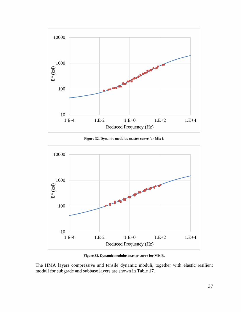
4.4.2. Material Characterization The lime-treated subbase and subgrade soil layers were characterized by Elastic moduli derived from the Falling Weight Deflectometer (FWD) tests. The HMA materials were characterized by Prony series and compressive dynamic moduli. The compressive dynamic moduli used were extracted from the master curves constructed based on dynamic modulus tests results. The master curves are given in Figures 31 to 33 at the reference temperature of 104°F (40°C). This temperature was close to the pavement temperature recorded during the field testing (Table 15). In order to determine the compressive dynamic modulus that represents the HMA pavement layer during field testing, a vehicle speed of 50 mph was used. In the laboratory, this speed is equivalent to 25 Hz (0.04 sec).

Figure 31. Dynamic modulus master curve for Mix S.

10

100

1000

10000

1.E-4 1.E-2 1.E+0 1.E+2 1.E+4

E* (k

si)

Reduced Frequency (Hz)

37

Figure 32. Dynamic modulus master curve for Mix I.

Figure 33. Dynamic modulus master curve for Mix B.

The HMA layers compressive and tensile dynamic moduli, together with elastic resilient moduli for subgrade and subbase layers are shown in Table 17.

10

100

1000

10000

1.E-4 1.E-2 1.E+0 1.E+2 1.E+4

E* (k

si)

Reduced Frequency (Hz)

10

100

1000

10000

1.E-4 1.E-2 1.E+0 1.E+2 1.E+4

E* (k

si)

Reduced Frequency (Hz)

38

Table 17. Layers moduli used in the FE model analysis.

Compressive-DM psi (MPa) Resilience Modulus psi (MPa) Surface (SMA) 519,960 (3585) N/A Binder (Type D) 544,762 (3756) N/A Base (Type B) 514,811 (3550) N/A Subbase N/A 80,000 (551) Subgrade N/A 8,000 (55)

To implement the compressive dynamic modulus of the HMA layers, a viscoelastic model was used. Abaqus/CAE uses a combination of viscoelastic Prony series and elastic model to represent the viscoelastic model.

Abaqus program has two options of implementing Prony series to define the viscoelastic time dependent properties of materials: time domain viscoelasticity and frequency domain viscoelasticity (19). The time domain option was used in the FE analysis to define the viscoelastic time dependent behavior of the asphalt mixes.

Three Prony series input parameters are needed for time domain viscoelasticity. These parameters are the dimensionless shear relaxation modulus (gi), the dimensionless bulk relaxation modulus (ki), and the reduced relaxation time (τi). The parameters are defined as:

𝑔𝑔𝑖𝑖 =𝐺𝐺𝑖𝑖𝐺𝐺0

[17]

where: 𝑔𝑔𝑖𝑖 = dimensionless shear relaxation modulus at time i, 𝐺𝐺𝑖𝑖 = shear relaxation modulus at time i, and 𝐺𝐺0 = initial shear relaxation modulus.

𝑘𝑘𝑖𝑖 =𝐾𝐾𝑖𝑖𝐾𝐾0

[18]

where: 𝑘𝑘𝑖𝑖 = dimensionless bulk relaxation modulus at time i, 𝐾𝐾𝑖𝑖 = bulk relaxation modulus at time i, and 𝐾𝐾0= initial bulk relaxation modulus.

The Prony series parameters were calculated by developing a Microsoft Excel spreadsheet to fit curves representing the models in Equations 17 and 18 to the computed shear modulus 𝐺𝐺𝑅𝑅(𝑡𝑡) and bulk relaxation modulus 𝐾𝐾𝑅𝑅(𝑡𝑡) data.

𝐺𝐺𝑅𝑅(𝑡𝑡) = 𝐺𝐺0(1 − 𝛴𝛴𝑖𝑖=1𝑁𝑁 𝑔𝑔𝑖𝑖𝑃𝑃(1− 𝑒𝑒−𝑡𝑡𝜏𝜏𝑖𝑖 )) [19]

39

𝐾𝐾𝑅𝑅(𝑡𝑡) = 𝐾𝐾0(1 − 𝛴𝛴𝑖𝑖=1𝑁𝑁 𝑘𝑘𝑖𝑖𝑃𝑃(1 − 𝑒𝑒−𝑡𝑡𝜏𝜏𝑖𝑖 )) [20]

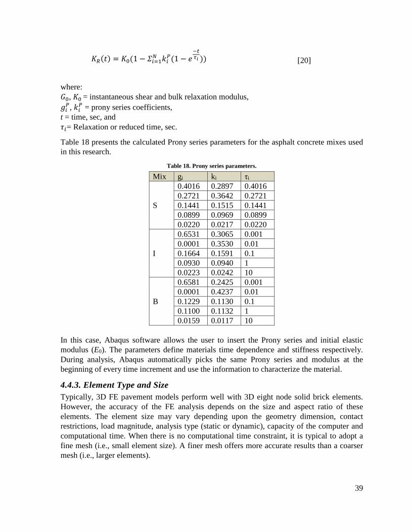
where: 𝐺𝐺0, 𝐾𝐾0 = instantaneous shear and bulk relaxation modulus, 𝑔𝑔𝑖𝑖𝑃𝑃, 𝑘𝑘𝑖𝑖𝑃𝑃 = prony series coefficients, t = time, sec, and 𝜏𝜏𝑖𝑖= Relaxation or reduced time, sec.

Table 18 presents the calculated Prony series parameters for the asphalt concrete mixes used in this research.

Table 18. Prony series parameters.

Mix gi ki τi S 0.4016 0.2897 0.4016 S 0.2721 0.3642 0.2721 S 0.1441 0.1515 0.1441 S 0.0899 0.0969 0.0899 S 0.0220 0.0217 0.0220 I 0.6531 0.3065 0.001 I 0.0001 0.3530 0.01 I 0.1664 0.1591 0.1 I 0.0930 0.0940 1 I 0.0223 0.0242 10 B 0.6581 0.2425 0.001 B 0.0001 0.4237 0.01 B 0.1229 0.1130 0.1 B 0.1100 0.1132 1 B 0.0159 0.0117 10

In this case, Abaqus software allows the user to insert the Prony series and initial elastic modulus (E0). The parameters define materials time dependence and stiffness respectively. During analysis, Abaqus automatically picks the same Prony series and modulus at the beginning of every time increment and use the information to characterize the material.

4.4.3. Element Type and Size Typically, 3D FE pavement models perform well with 3D eight node solid brick elements. However, the accuracy of the FE analysis depends on the size and aspect ratio of these elements. The element size may vary depending upon the geometry dimension, contact restrictions, load magnitude, analysis type (static or dynamic), capacity of the computer and computational time. When there is no computational time constraint, it is typical to adopt a fine mesh (i.e., small element size). A finer mesh offers more accurate results than a coarser mesh (i.e., larger elements).

40

Abaqus requires that the aspect ratio (ratio between the longest and shortest edge of an element), to be less than 10 for accurate results. However, an aspect ratio of less or equal to 4 is recommended for areas around the loaded area (i.e., wheel path) (19).

In order to achieve optimum accuracy without increasing the computational cost, a biased mesh was used. Small elements were used in the HMA layer along the wheel path where high stress-strain gradients occur, and increasingly large element size were used far away from the loading path.

A convergence test was performed using a static load to determine the optimal number of elements needed. After convergence test, it was determined that 1.0 x 2-inches elements were suitable for the area around the wheel path. 2 x 5-inches and 2 x 10-inches element sizes were used toward the far ends. All elements used in the model were type C3D8R except for the sides away from the symmetry plane of the model where infinite element type CIN3D8 were used (Figure 34).

Figure 34. Element type and size.

The C3D8R element is a solid eight-node linear brick element with reduced integration. Due to reduced integration, the element offers relatively low computational cost. However, because its integration point is located at the middle of the element, small elements are usually required for accurate results (Figure 35a). A special case of the C3D8R elements is CIN3D8. The CIN3D8 elements have five finite solid faces and one infinite face (Figure 35b). FE programs use CIN3D8 elements to represent far-field regions of continuous structures such as pavements. Abaqus/CAE does not support infinite elements in its current setting. However, these elements were included in the input file using a text editor.

41

Figure 35. The elements used (a) C3D8R Finite and (b) CIN3D8 Infinite.

4.4.4. Boundary Conditions In this research, three different types of boundary conditions were employed to represent the pavement end supports.

Infinite boundaries: this type of boundary was assigned to three vertical sides far from the loading area (Figure 36). The boundaries allow reduction of elements that would have been used to extend the model far from the dynamical loaded area. They do so by offering a smooth decay of stresses to the far ends of the model geometry.

Z-Asymmetry: in order to take advantage of symmetry of the geometry and loading only a half of the pavement structure was modeled. To do so, the horizontal movement of the nodes in the symmetry plane was restricted (Figure 36).

Fixed end: The movement of the nodes at the bottom of the pavement structure (located 120-inches from the surface) was restricted in all directions. (Figure 36).

Figure 36. Boundary conditions of the model.

42

4.4.5. Loading Tire Imprint: the tire imprint is the contact area between the tire and pavement surface. The size of tire imprint depends on contact pressure, which is often assumed equal to the tire inflation pressure. In this case, the tire inflation pressure and wheel load are used to calculate the size of tire imprint. However, the dimensions of the tire imprints were measured in the US-287 pavement project when the pavement response measurements were conducted. The tire imprint dimensions used in this research are shown in Figure 37.

Figure 37. Tire imprint dimensions.

Surface Partitions: there are two ways in which external loads may be applied to an Abaqus model: element loading or surface loading. Since the research used more than 600 surfaces to define the vehicle moving load, the surface loading procedure was selected to avoid redefining of the loaded surfaces when element size changes. The surfaces along which the truck tires passed were partitioned into small spaces in relation to the widths of rear and steering tire imprints. In addition, a few more partition lines along the length were added to allow for repositioning of the wheels when necessary (Figure 38).

Simulation of Moving Loads: in the Abaqus FE model, traffic loads may be applied statically or dynamically. In this research, dynamic moving wheel loads were modeled by implementing the concept of step loading with trapezoidal loading amplitude. There are three main components of this concept: the entry surface segment (or element), the tire imprint segments and the leaving segment (element). When a vehicle approaches a given surface segment, the surface is loaded with amplitude that increases linearly from 0 to 1. Similarly, as the tire moves

43

away from a given surface segment, the loading amplitude that simulates the decrease in loading from 1 to 0 is used. The surface segments within the tire imprint are loaded with constant loading amplitude of 1. Table 19 and Figure 39 show the transition of wheel load from step-1 to step-2, step-2 to step-3 and so on, along the wheel path.

Figure 38. Wheel path surface partition.

Table 19. Wheel load transition parameters.

Load Position Surface Amplitude Step 1 Leave S1 1 to 0 Step 1 Tire Imprint S2 1 to 1 Step 1 Entry S3 0 to 1 Step 2 Leave S2 1 to 0 Step 2 Tire Imprint S3 1 to 1 Step 2 Entry S4 0 to 1 Step 3 Leave S3 1 to 0 Step 3 Tire Imprint S4 1 to 1 Step 3 Entry S5 0 to 1 Step 4 Leave S4 1 to 0 Step 4 Tire Imprint S5 1 to 1 Step 4 Entry S6 0 to 1

44

Figure 39. Schematic of a moving tire based on the trapezoidal loading method.

The duration of each step or step time was calculated based on the speed of the vehicle and the length of the surface segment along the direction of travel. At first, the speed was converted from miles per hour into inches per second. Then the size of each segment on the wheel path was divided by the speed in inches per second to obtain the time required for each step to move the load at the desired speed. In this model, the length of surface segment used to advance a wheel load from one-step to the next was 2 inches. To model the load moving at 50 mph, which is equals to 880 inches per second, the 2 inches was divided by 880 inches per second, and a step time of 0.002273 seconds was obtained. Thereafter, loading amplitudes were created using the tabular option in ABAQUS. Table 20 presents the tabular data used to create the loading amplitudes for 50 mph speed.

Table 20. Loading amplitude tabular data for 50 mph.

Entry Surface Segment

Step Time (s)

Entry Surface Segment

Amplitude

Within Tire Imprint

Step Time (s)

Within Tire Imprint

Amplitude

Leaving Surface Segment

Step Time (s)

Leaving Surface Segment

Amplitude 0 0 0 1 0 1

0.002273 1 0.002273 1 0.002273 0

The total step time used was further divided into small segments (time increments) to allow for the solution to converge. Abaqus has two options of implementing time increments: automatic or fixed by the user. Abaqus recommends the automatic method to avoid convergence problems. Table 23 shows the load amplitude data with the sub-divided time steps.

45

5. FINDINGS 5.1. Response Data Analysis All strain signals recorded under the passing of the loading vehicle are given in Appendix A. The signals followed a pattern very similar to that shown in Figure 40. For each signal, the values recorded in several points (A to H) on the signal were extracted. The points were as follows:

• A: the initial value before the vehicle arrived. It is 0.0 for all signals since this value was the starting point for all signals.

• B: the maximum strain value recorded under the front (steering wheel) • C: the smallest value after the passing of the front wheel and the arrival of the rear

wheel. • D: the maximum strain value recorded under the first real wheel (of the tandem axle) • E: the smallest value after the passing of the first wheel and the second wheel of the

rear (tandem) axle. • F: the maximum strain value recorded under the second real wheel (of the tandem axle). • G: the smallest value after the passing of the second wheel of the rear axle. • H: the strain value recorded 0.5 second after the passing of the second real wheel.

Figure 40. Example strain signal.

It is important to observe that the values for C and G are almost always negative for the longitudinal strain signals and positive for transverse strain signals. This is expected since the longitudinal strain recovers after the passing of each wheel but the transverse strain does not.

The values A to H were extracted for all strain signals in Tables 21 and 22. The tables indicate the following:

46

• For both longitudinal and transverse strains, the corresponding values varied greatly from one pass of the vehicle to another. This can be explained the variation of the lateral position of the vehicle relative to the location of the gauges.

• Even for gauges located in the same lateral position and measuring the strain in the same direction (e.g., T1 and T3), the recorded strain values were not the same. This may be explained by the insufficient bond between the gauge and the core or between the core and the surrounding concrete. Therefore, it was decided to retain the strain values only for the gauges that recorded the highest strain values for the same lateral position and direction. These gauges are: T3, T5, L2 and L8.

• In general, the recorded strains were very small, always less than 25 microstrain, much less than 70 microstrain considered as the endurance limit for asphalt concrete. This suggests that the thick lime-treated embankment layer significantly improved the bearing capacity of the pavement structure that will likely never exhibit bottom-up cracking.

• Gauge T7 exhibited irregular strain signal, possibly because of improper bond between the gauge and the core it is attached to.

• For the instrumented pavement structure, the compounding effect of the transverse strain from the front and the rear axle was minimal. The low values of parameter C in Table 22 indicate that the transverse strain recovered almost entirely after the passing of the front wheel before the rear wheel arrived.

Figures 41 to 43 show the measured strains under the pass of the steering wheel and the two rear wheels. The position is reported for each pass in Table 15. The figures reveal that for most passes, the wheels passed to the right of the alignment where the sensors were installed, that is closer to the shoulder. They also indicate that, with a few exceptions, the transverse strains are slightly higher than the longitudinal strains for the same wheel, sensor position and vehicle pass. Both Tables 21 and 22 and Figures 41 to 43 indicate that the strains induced at the bottom of the asphalt layer by the front wheel of the vehicle is of comparable magnitude to the strain induced by the wheels of the real axles. This suggests that the front wheels should be considered when computing the fatigue damage at the bottom of the asphalt layer.

47

Table 21. Measured transverse strain values.

Pass Sensor A B C D E F G H 1 T1 0 2.2 0 6 1.3 5.1 0.2 0.1 1 T3 0 4.7 0.7 13.1 2.7 12.1 0.6 0.5 1 T5 0 8.8 1.3 14 3.2 13.4 3 3.1 1 T7 0 5.1 0 2.4 0.5 3.6 -1.7 1.7 2 T1 0 2.1 0 6 1.4 4.4 0.2 0.1 2 T3 0 4.3 0.7 10.3 2.5 8.8 1.0 3.0 2 T5 0 8.2 -0.6 12.2 1.8 11.3 1.3 1.1 2 T7 0 6.0 -0.2 2.5 0.5 3.6 -0.1 0.2 3 T1 0 9.0 0.4 6.2 1.4 7.2 1.6 0 3 T3 0 22.0 1.4 7.7 1.7 13 1.3 0 3 T5 0 12.9 -3.4 13.5 0.6 17.3 1.0 -0.1 4 T1 0 1.1 0 3.7 0.7 2.7 0 0 4 T3 0 2.4 0.3 9 2.5 5.9 1.3 0.2 4 T5 0 2.1 -0.9 10.4 2.2 7.7 1.2 1 5 T1 0 4.0 0 7.9 1.2 7 0.8 0 5 T3 0 8.3 1.1 17.7 3.2 12.8 0.5 0.4 5 T5 0 16.1 0.1 10.5 1.4 10 1.3 1.0 5 T7 0 6.1 0 1.3 0.1 2.8 -0.1 0 6 T1 0 1.8 -0.1 4.3 0.6 3.3 0.4 0 6 T3 0 3.2 0.5 12.7 2.6 8.1 0.4 0.4 6 T5 0 5.4 -1.5 10.7 1.3 9.3 -0.3 1.3 6 T7 0 4.4 -0.5 2.9 0.1 3.1 -0.3 0 7 T1 0 2.4 0 7.3 2.0 5.9 0.6 0.2 7 T3 0 5.3 0.8 17.5 3.4 12.7 1.4 0.2 7 T5 0 10.8 -0.8 10.8 1.4 9.6 0.7 0.8 7 T7 0 5.8 0 1.9 0.6 3.2 0.3 2.0

48

Table 22. Measured longitudinal strain values.

Pass Sensor A B C D E F G H 1 L2 0 1.8 -0.4 8.9 2.5 6.8 0.2 0.5 1 L4 0 2.7 -0.3 1.1 -0.5 1.4 -0.4 0 1 L6 0 4.8 -1.3 11.1 0.5 8.7 -1.1 0.4 1 L8 0 6.5 -4.6 17.7 -6.7 11.7 -7.8 0.4 2 L2 0 1.5 -0.1 6.7 1.7 5.1 0 0 2 L4 0 0.2 -0.2 1.4 -0.3 0.9 -0.7 0 2 L6 0 4.3 -1.4 10.4 0.6 8.3 -2.2 0 2 L8 0 7.2 -4.7 15.1 -5.9 10.8 -8.1 0 3 L2 0 17.1 0.9 10.8 1.6 10.4 0 0.6 3 L4 0 5.3 -0.7 5.2 -0.8 4.1 -1 0 3 L6 0 13.2 -0.1 12.2 0.9 12.1 -0.9 0.2 3 L8 0 19.5 -7.9 19.2 -8.6 20.2 -12.6 0 4 L2 0 0.8 -0.2 5.8 1.1 3.4 0.3 0.3 4 L4 0 0.2 -0.1 1.1 -0.1 0.5 -0.2 0.3 4 L6 0 2.2 -2 8 -0.9 4.9 -1.9 -0.6 4 L8 0 2.4 -3.4 10.1 -4.4 6.6 -6 -0.6 5 L2 0 4.2 0 16.2 2.2 9.6 -0.1 0 5 L4 0 0.1 -0.2 5.1 -0.4 2.1 -0.1 0 5 L6 0 8.6 -1.6 9.3 0 7.4 -1.4 0 5 L8 0 11.2 -6.8 13.2 -5.8 10.2 -7.6 0 6 L2 0 1 -0.9 7.2 1.6 4 0 -0.9 6 L4 0 0 -0.5 1.5 -0.4 0.6 -0.2 -1 6 L6 0 3.4 -1.6 9.8 0.1 5.6 -1.1 0 6 L8 0 4.6 -3.3 12.4 -4 8.3 -6.2 0 7 L2 0 2.1 -0.7 13.8 2.1 7.5 0.5 0.1 7 L4 0 0 -0.4 3.5 -0.3 1.1 -0.6 0 7 L6 0 5.3 -1.6 10 0.1 6.6 -1.4 0 7 L8 0 7.2 -4.4 13.7 -4.5 9.6 -7.1 0

49

Figure 41. Measured strains under the steering wheel.

Figure 42. Measured strains under the first rear wheel.

0

5

10

15

20

25

-14 -12 -10 -8 -6 -4 -2 0 2 4

Stra

in (m

icro

stra

in)

Distance from Sensor to Center of Steering Wheel (inches)

Strain under the Steering Wheel

Transverse

Longitudinal

0

5

10

15

20

25

-14 -12 -10 -8 -6 -4 -2 0 2 4

Stra

in (m

icro

stra

in)

Distance from Sensor to Center of Rear Wheel (inches)

Strain under the First Rear Wheel

Transverse

Longitudinal

50

Figure 43. Measured strains under the second rear wheel.

5.2. Results of the Finite Element Analysis After the finite element model was run the variation in time of the longitudinal and transverse strains were extracted for 24 elements located at the bottom of the base layer in the vicinity of the loaded elements. Figure 44 shows an example of such strain curves obtained for one element. It can be observed that the computed longitudinal strain recovers and becomes negative (compressive) after the passing of the steering axle and after the passing of the rear axle. However, after the computed transverse strains remain always positive (tensile) throughout the duration of loading. This pattern is the same as the one observed on the measured strain signals.

The same as for the measured strains, the values A to H were extracted for all strain signals; they are given in Tables 19 and 20. To locate the elements in relation to the transverse position of the wheels, the center of the rear wheel is between elements E-1 and E1. The elements with a positive name, such as E4, are located to the right of the center of the rear wheel. The tables also give the transverse distances between the center of each element and the centers of the steering and rear wheels; the distance is positive if the center of the element is to the right of the center of the wheel.

0

5

10

15

20

25

-14 -12 -10 -8 -6 -4 -2 0 2 4

Stra

in (m

icro

stra

in)

Distance from Sensor to Center of Rear Wheel (inches)

Strain under the Second Rear Wheel

Transverse

Longitudinal

51

Table 23. Subdivided Loading Amplitude Tabular Data for 50 mph.

Entry Surface segment Step Time (s)

Entry Surface segment Amplitude

Within Tire Imprint -Step Time (s)

Within Tire Imprint -Amplitude

Leaving Surface Segment-Step Time (s)

Leaving Surface Segment- Amplitude

0.00E+00 0 0.00E+00 1 0.00E+00 1 1.14E-04 0.05 1.14E-04 1 1.14E-04 0.95 2.27E-04 0.1 2.27E-04 1 2.27E-04 0.9 3.41E-04 0.15 3.41E-04 1 3.41E-04 0.85 4.55E-04 0.2 4.55E-04 1 4.55E-04 0.8 5.68E-04 0.25 5.68E-04 1 5.68E-04 0.75 6.82E-04 0.3 6.82E-04 1 6.82E-04 0.7 7.96E-04 0.35 7.96E-04 1 7.96E-04 0.65 9.09E-04 0.4 9.09E-04 1 9.09E-04 0.6 1.02E-03 0.45 1.02E-03 1 1.02E-03 0.55 1.14E-03 0.5 1.14E-03 1 1.14E-03 0.5 1.25E-03 0.55 1.25E-03 1 1.25E-03 0.45 1.36E-03 0.6 1.36E-03 1 1.36E-03 0.4 1.48E-03 0.65 1.48E-03 1 1.48E-03 0.35 1.59E-03 0.7 1.59E-03 1 1.59E-03 0.3 1.70E-03 0.75 1.70E-03 1 1.70E-03 0.25 1.82E-03 0.8 1.82E-03 1 1.82E-03 0.2 1.93E-03 0.85 1.93E-03 1 1.93E-03 0.15 2.05E-03 0.9 2.05E-03 1 2.05E-03 0.1 2.16E-03 0.95 2.16E-03 1 2.16E-03 0.05 2.27E-03 1 2.27E-03 1 2.27E-03 0

52

Table 24. Transverse strains computed by the FE model (A-H are significance values shown in Figure 28).

Element Element Width (in.)

Center of Front Axle

Center of Rear Axle

A B C D E F G H

E-10 2.45 -23.58 -20.325 0.00 0.50 -0.59 1.33 0.42 1.26 -0.48 -0.36 E-9 2.45 -21.13 -17.875 0.00 0.57 -0.35 1.49 0.99 1.80 0.47 -0.30 E-8 2.45 -18.68 -15.425 0.00 0.67 -0.17 1.95 1.74 2.31 -0.41 -0.24 E-7 2.45 -16.23 -12.975 0.00 0.83 0.18 2.85 2.56 3.00 -0.28 -1.09 E-6 1.9 -14.05 -10.800 0.00 1.06 0.45 3.74 3.02 3.60 -0.22 -0.06 E-5 1.9 -12.15 -8.900 0.00 1.43 0.89 4.35 3.32 4.34 -0.16 -0.06 E-4 1.9 -10.25 -7.000 0.00 1.76 0.83 4.77 3.68 4.86 -0.06 0.00 E-3 1.9 -8.35 -5.100 0.00 2.42 0.91 5.02 3.80 5.12 0.00 0.00 E-2 1.9 -6.45 -3.200 0.00 3.13 1.07 5.04 4.16 5.05 0.00 0.12 E-1 2.25 -4.38 -1.125 0.00 4.04 1.07 5.00 4.28 5.00 0.00 0.12 E1 2.25 -2.13 1.125 0.00 4.68 1.06 5.00 4.28 5.07 0.00 0.12 E2 1.3 -0.35 2.900 0.00 5.01 1.18 5.18 4.17 5.12 0.12 0.12 E3 1.3 0.95 4.200 0.00 4.95 1.06 5.19 4.05 5.13 0.12 0.12 E4 1.3 2.25 5.500 0.00 4.75 1.06 5.16 4.04 5.12 0.12 0.12 E5 1.3 3.55 6.800 0.00 4.37 1.07 5.07 3.92 5.00 0.12 0.12 E6 1.3 4.85 8.100 0.00 3.86 1.04 4.82 3.68 4.86 -0.06 0.12 E7 1 6.00 9.250 0.00 3.46 0.94 4.58 3.40 4.48 -0.06 -0.03 E8 1 7.00 10.250 0.00 3.04 0.94 4.18 3.32 4.05 -0.12 -0.03 E9 1 8.00 11.250 0.00 2.55 0.93 3.77 3.10 3.72 -0.15 -0.04 E10 1.5 9.25 12.500 0.00 2.28 0.83 3.23 2.95 3.27 -0.20 -0.09 E11 1.75 10.88 14.125 0.00 1.64 0.82 2.69 2.41 2.83 -0.28 -0.14 E12 2 12.75 16.000 0.00 1.45 0.71 1.90 1.67 2.47 -0.35 -0.15 E13 2.25 14.88 18.125 0.00 1.10 0.52 1.54 1.04 1.86 -0.35 -0.16 E14 2.5 16.13 20.750 0.00 0.85 0.17 1.28 0.59 1.45 -0.41 -0.24

53

Figure 44. Computed strain signals at the bottom of HMA layer.

5.3. Comparison of Measured and Computed Strains Figures 45 to 47 compare the field-measured and FE computed strains at the bottom of the HMA layers. The magnitude of the strains is shown in relation to the transverse distance between the points where the strains were computed and measured and the centers of the steering wheel and the rear wheels.

The charts prove that the computed strains have similar magnitude to the measured strains. All strains are small, less than 25 microstrain. They also indicate that the maximum computed longitudinal and transverse strains under the steering wheel are about the same. However, under the rear wheel, the maximum computed longitudinal strains are larger than the computed maximum transverse strains. The opposite was observed for the measured strains. The charts also indicate that the computed strains fall in the middle of the range of the measured strains for the strains under the steering wheel and the second rear wheel. For the first rear wheel, the computed strains are at the bottom of the range of measured strains.

-2.E-06

-1.E-06

0.E+00

1.E-06

2.E-06

3.E-06

4.E-06

5.E-06

6.E-06

7.E-06

0 0.1 0.2 0.3 0.4 0.5 0.6 0.7 0.8 0.9

Stra

in

Time (seconds)

Finite Element Computed Strain Signals

Longitudinal

Transverse

54

Table 25. Longitudinal strains computed by the FE Model (A-H are significance values shown in Figure 28).

Element Element Width (in.)

Center of Front Axle

Center of Rear Axle

A B C D E F G H

E-10 2.45 -23.58 -20.325 0.00 2.37 -1.31 4.03 1.95 4.04 -1.00 0.12 E-9 2.45 -21.13 -17.875 0.00 2.60 -1.31 4.41 1.79 4.27 -1.06 0.12 E-8 2.45 -18.68 -15.425 0.00 2.86 -1.36 4.77 1.55 4.74 -1.11 0.12 E-7 2.45 -16.23 -12.975 0.00 3.00 -1.36 5.12 1.41 5.20 -1.10 0.12 E-6 1.9 -14.05 -10.800 0.00 3.22 -1.36 5.58 1.13 5.36 -0.98 0.12 E-5 1.9 -12.15 -8.900 0.00 3.58 -1.36 5.59 1.11 5.64 -1.10 0.12 E-4 1.9 -10.25 -7.000 0.00 3.87 -1.30 5.95 0.87 5.84 -1.07 0.12 E-3 1.9 -8.35 -5.100 0.00 4.17 -1.36 6.67 0.87 5.97 -1.00 0.12 E-2 1.9 -6.45 -3.200 0.00 4.53 -1.30 6.07 0.74 5.95 -1.05 0.12 E-1 2.25 -4.38 -1.125 0.00 4.89 -1.35 5.93 0.74 5.96 -1.11 0.12 E1 2.25 -2.13 1.125 0.00 5.13 -1.30 6.15 0.62 6.04 -1.03 0.12 E2 1.3 -0.35 2.900 0.00 5.13 -1.24 6.02 0.74 6.03 -1.02 0.12 E3 1.3 0.95 4.200 0.00 5.13 -1.30 6.01 0.74 5.99 -0.98 0.12 E4 1.3 2.25 5.500 0.00 5.00 -1.30 5.91 0.62 5.85 -1.00 0.12 E5 1.3 3.55 6.800 0.00 4.88 -1.24 5.77 0.86 5.70 -1.03 0.12 E6 1.3 4.85 8.100 0.00 4.77 -1.28 5.64 0.74 5.57 -0.95 0.12 E7 1 6.00 9.250 0.00 4.53 -1.23 5.55 0.87 5.44 -0.89 0.12 E8 1 7.00 10.250 0.00 4.29 -1.24 5.28 0.87 5.10 -1.03 0.12 E9 1 8.00 11.250 0.00 4.17 -1.21 5.15 0.87 5.11 -1.00 0.12 E10 1.5 9.25 12.500 0.00 3.93 -1.21 4.92 1.00 4.89 -0.88 0.12 E11 1.75 10.88 14.125 0.00 3.48 -1.17 4.73 1.14 4.66 -0.85 0.12 E12 2 12.75 16.000 0.00 3.20 -1.20 4.36 1.19 4.16 -0.82 0.12 E13 2.25 14.88 18.125 0.00 2.90 -1.45 3.90 1.43 3.81 -0.83 0.12 E14 2.5 16.13 20.750 0.00 2.70 -1.10 3.55 1.61 3.58 -0.74 0.12

55

Figure 45. Measured versus estimated strains under the steering wheel.

Figure 46. Measured versus estimated strains under the first rear wheel.

0

5

10

15

20

25

-25 -20 -15 -10 -5 0 5 10 15 20

Stra

in (m

icro

stra

in)

Distance from Sensor to Center of Steering Wheel (inches)

Strain under the Steering Wheel

TransverseLongitudinalFE-TransverseFE-Longitudinal

0

5

10

15

20

25

-25 -20 -15 -10 -5 0 5 10 15 20 25

Stra

in (m

icro

stra

in)

Distance from Sensor to Center of Rear Wheel (inches)

Strain under the First Rear Wheel

TransverseLongitudinalFE-TransverseFE-Longitudinal

56

Figure 47. Measured versus estimated strains under the second rear wheel.

0

5

10

15

20

25

-25 -20 -15 -10 -5 0 5 10 15 20 25

Stra

in (m

icro

stra

in)

Distance from Sensor to Center of Rear Wheel (inches)

Strain under the Second Rear Wheel

TransverseLongitudinalFE-TransverseFE-Longitudinal

57

6. CONCLUSIONS In order to estimate the damage caused by heavy vehicles on flexible pavement structures, a newly constructed pavement was instrumented with strain gauges retrofitted at the bottom of the asphalt concrete base layer to measure longitudinal and transverse strains. The instrumented section is located on highway US-287, to the South of Mansfield, TX. The road has a medium to heavy truck traffic and opened to traffic in July 2018.

The strain gauges were used to measure the strains under several passes of a test vehicle which had a steering axle with single tire for each wheel and a rear tandem axle with dual tires. The speed and the lateral position of the vehicle were recorded for each pass by photographic means. Sufficient quantities of the top two layers of asphalt concrete were obtained during construction and were used to fabricate cylindrical samples for conducting the dynamic modulus test in the laboratory. The dynamic moduli test results were used to determine the viscoelastic properties of the two mixes.

The general-purpose finite element program Abaqus was used to model the instrumented pavement section and to compute the longitudinal and transverse strains. The asphalt mixes were modeled as visco-elastic materials having the properties determined by the dynamic modulus tests. The wheel loads were modeled as pressure elements applied at the top of the modeled structure in time step increments. The time evolutions of the longitudinal and transverse strains were extracted for 24 elements located at the bottom of the asphalt concrete base layer. The computed strain data were compared to the field measured strain data.

The analysis of the measured responses led to the following major conclusions: • The measured transverse strains were most of the time slightly larger than the

corresponding longitudinal strains. This can be attributed to the accumulation of strain from the front axle and the rear axle that takes place only in the transverse direction. However, the finite element model computed higher strains in the longitudinal direction than in the transverse direction.

• For both measured and computed strains, the values under the passing of the steering wheel were of similar size as the strains under the passing of the first wheel of the rear axle.

• The measured longitudinal and transverse strains were always lower than 25 microstrain, much lower than the 70 microstrain, the average endurance limit value reported in the literature, despite the high temperature in the asphalt layers during the measurements.

• The measured strains exhibited high variation, not only between the values recorded by the gauges placed in the same transverse location but also between the values recorded for different passes of the test vehicle.

58

7. RECOMMENDATIONS The results of the field experiment and of the finite element analysis recommend the following:

• Both longitudinal and transverse strains should be used in the estimation of damage induced by passing of heavy vehicles and not only the longitudinal strains as is currently done by most distress prediction models.

• The damage induced by the single tire steering axle should also be included in the damage calculations. For many trucks, the load on the steering axle is quite large, more than 5,000 lbf per wheel. Since steering wheels have a single tire, the strains generated in the asphalt layers are comparable to the strains generated by the rear axles.

• The strains recorded and computed at the bottom of the asphalt concrete base layer for the studied pavement section were very low, less than 25 microstrain. Therefore, it is likely that the asphalt layer will not exhibit any bottom-up fatigue cracking during their design life. This may be due to the 36-inch-thick layer of lime treated soil. The use of thick stabilized subbase layers should be further studied since they may provide a significant increase to the structural capacity of the pavement section at a relatively low cost.

59

REFERENCES 1. Finn, F.N. Factors Involved in the Design of Asphaltic Pavement Surfaces. NCHRP Report 39, Transportation Research Board, National Research Council, Washington, DC, 1967.

2. Asphalt Institute. Asphalt Pavements for Highways and Streets, Asphalt Institute Manual Series-1 (MS-1), 9th Edition, Asphalt Institute, Lexington, KY, 1981.

3. AASHTO. Mechanistic-Empirical Pavement Design Guide: A Manual of Practice. Second Edition, American Association of State Highway and Transportation Officials, Washington, DC, 2015.

4. Miner, M.A. (1945), Cumulative Damage in Fatigue, Transactions of the ASCE, Vol. 67, pp. A159-A164.

5. Bao, W. Calibration of Flexible Pavements Structural Model Using Mn/Road Data. M.S thesis, University of Minnesota-Twin Cities, Minnesota, 2000.

6. Lukanen, E. O. Load Testing of Instrumented Pavement Sections. Minnesota DOT Report, MN/RC-2005-47, Minnesota Department of Transportation, Twin Cities, MN, 2005.

7. Appea, A.K. Validation of FWD Testing Results at the Virginia Smart Road: Theoretically and by Instrument Responses. PhD Dissertation, Virginia Polytechnic Institute and State University, Blacksburg, VA, 2003.

8. Timm, D, Priest A. and McEwen T. “Design and Instrumentation of the Structural Pavement Experiment at The NCAT Test Track”. NCAT Report 04-01, National Center for Asphalt Technology, Opelika, AL, 2004.

9. Loulizi, A. I., Al Qadi, S. Lahouar and Freeman T. “Data Collection and Management of Instrumented Smart Road Flexible Sections” In Transportation Research Record No. 1769, Transportation Research Board, National Research Council, Washington, D.C., 2001, pp., 142-151.

10. Romanoschi, S.A., A. J. Gisi, M. Portillo and Dumitru C. “The First Findings from the Kansas Perpetual Pavements Experiment”. In Transportation Research Record No. 2068, Transportation Research Board, National Research Council, Washington, D.C., 2008, pp. 41-48.

11. Bayat, A. and M.A. Knight “Investigation of Flexible Pavement Structural Response for the Centre for Pavement and Transportation Technology (CPATT) Test Road.” In Proceedings of the Transportation Research Board 89th Annual Meeting (DVD), Washington, DC, January 10 to 14, 2010.

12. Knight M., Tighe S. and Adedapo A. “Trenchless Installations Preserve Pavement Integrity”, In the Proceedings of the Annual Conference of the Transportation Association of Canada, Quebec City, 2004.

60

13. ASTM 1049-85. Standard Practices for Cycle Counting in Fatigue Analysis, American Society for Testing of Materials, Washington, DC, 2017.

14. Papagiannakis, A.T., A.Oancea, N.Ali and Chan J. "Application of ASTM E 1049-85 in Calculating Vehicle Equivalence Factors from In-situ Strains". In Transportation Research Record No. 1307, Transportation Research Board, National Research Council, Washington, D.C., 1992, pp. 82-89.

15. TxDOT Standard Specifications for Construction and Maintenance of Highways, Streets and Bridges. https://www.txdot.gov/business/resources/txdot-specifications.html. Accessed January 25, 2018.

16. Witczak M.W., Kaloush K., Pellinen T., El-BAsyouny M. and Von Quintus H. Simple Performance Test for Permanent Deformation Based upon Dynamic Modulus of Asphalt Concrete Mixtures. NCHRP Report 465, National Cooperative Highway Research Program, Transportation Research Board, National Research Council, Washington, DC, 2002.

17. LTPP Computed Parameter: Dynamic Modulus. September 2011. https://www.fhwa.dot.gov/publications/research/infrastructure/pavements/ltpp/10035/002.cfm. Accessed October 5, 2017.

18. Tokyo-Sokki Kenkyujo Co., TML Embedment Strain Gauge. Type KM-100HAS. http://www.tml.jp/e/product/strain_gauge/gauge_list/index.html. Accessed July 2017.

19. Simulia ABAQUS 2016 User’s Guide. http://130.149.89.49:2080/v2016/index.html. Accessed May 18, 2018.

61

APPENDIX A: MEASURED STRAIN SIGNALS

Figure A-1. Transverse strain T1-T3, pass 1.

Figure A-2. Transverse strain T5-T7, pass 1.

-2.0

0.0

2.0

4.0

6.0

8.0

10.0

12.0

14.0

0 0.4 0.8 1.2 1.6 2

Stra

in

(m

icro

stra

in)

Time (seconds)

Transverse Strain - Pass 1

T1

T3

-4.0

-2.0

0.0

2.0

4.0

6.0

8.0

10.0

12.0

14.0

16.0

0 0.4 0.8 1.2 1.6 2

Stra

in

(m

icro

stra

in)

Time (seconds)

Transverse Strain - Pass 1

T5

T7

62

Figure A-3. Transverse strain T1-T3, pass 2.

Figure A-4. Transverse strain T5-T7, pass 2.

-2.0

0.0

2.0

4.0

6.0

8.0

10.0

12.0

0 0.4 0.8 1.2 1.6 2

Stra

in

(m

icro

stra

in)

Time (seconds)

Transverse Strain - Pass 2

T1

T3

-2.0

0.0

2.0

4.0

6.0

8.0

10.0

12.0

14.0

0 0.4 0.8 1.2 1.6 2

Stra

in

(m

icro

stra

in)

Time (seconds)

Transverse Strain - Pass 2

T5

T7

63

Figure A-5. Transverse strain T1-T3, pass 3.

Figure A-6. Transverse strain T5-T7, pass 3.

-5.0

0.0

5.0

10.0

15.0

20.0

25.0

0 0.4 0.8 1.2 1.6 2

Stra

in

(m

icro

stra

in)

Time (seconds)

Transverse Strain - Pass 3

T1

T3

-10.0

-5.0

0.0

5.0

10.0

15.0

20.0

0 0.4 0.8 1.2 1.6 2Stra

in

(m

icro

stra

in)

Time (seconds)

Transverse Strain - Pass 2

T5

T7

64

Figure A-7. Transverse strain T1-T3, pass 4.

Figure A-8. Transverse strain T5-T7, pass 4.

-2.0

0.0

2.0

4.0

6.0

8.0

10.0

0 0.4 0.8 1.2 1.6 2

Stra

in

(m

icro

stra

in)

Time (seconds)

Transverse Strain - Pass 4

T1

T3

-25.0

-20.0

-15.0

-10.0

-5.0

0.0

5.0

10.0

15.0

0 0.4 0.8 1.2 1.6 2

Stra

in

(m

icro

stra

in)

Time (seconds)

Transverse Strain - Pass 4

T5

T7

65

Figure A-9. Transverse strain T1-T3, pass 5.

Figure A-10. Transverse strain T5-T7, pass 5.

-2.0

0.0

2.0

4.0

6.0

8.0

10.0

12.0

14.0

16.0

18.0

20.0

0 0.4 0.8 1.2 1.6 2

Stra

in

(m

icro

stra

in)

Time (seconds)

Transverse Strain - Pass 5

T1

T3

-2.0

0.0

2.0

4.0

6.0

8.0

10.0

12.0

14.0

16.0

18.0

0 0.4 0.8 1.2 1.6 2

Stra

in

(m

icro

stra

in)

Time (seconds)

Transverse Strain - Pass 5

T5

T7

66

Figure A-11. Transverse strain T1-T3, pass 6.

Figure A-12. Transverse strain T5-T7, pass 6.

-2.0

0.0

2.0

4.0

6.0

8.0

10.0

12.0

14.0

0 0.4 0.8 1.2 1.6 2

Stra

in

(m

icro

stra

in)

Time (seconds)

Transverse Strain - Pass 6

T1

T3

-4.0

-2.0

0.0

2.0

4.0

6.0

8.0

10.0

12.0

0 0.4 0.8 1.2 1.6 2

Stra

in

(m

icro

stra

in)

Time (seconds)

Transverse Strain - Pass 6

T5

T7

67

Figure A-13. Transverse strain T1-T3, pass 7.

Figure A-14. Transverse strain T5-T7, pass 7.

-2.0

0.0

2.0

4.0

6.0

8.0

10.0

12.0

14.0

16.0

18.0

20.0

0 0.4 0.8 1.2 1.6 2

Stra

in

(m

icro

stra

in)

Time (seconds)

Transverse Strain - Pass 7

T1

T3

-2.0

0.0

2.0

4.0

6.0

8.0

10.0

12.0

0 0.4 0.8 1.2 1.6 2

Stra

in

(m

icro

stra

in)

Time (seconds)

Transverse Strain - Pass 7

T5

T7

68

Figure A-15. Longitudinal strain L2-L4, pass 1.

Figure A-16. Longitudinal strain L6-L8, pass 1.

-2.0

0.0

2.0

4.0

6.0

8.0

10.0

0 0.4 0.8 1.2 1.6 2

Stra

in

(m

icro

stra

in)

Time (seconds)

Longitudinal Strain - Pass 1

L2

L4

-10.0

-5.0

0.0

5.0

10.0

15.0

20.0

0 0.4 0.8 1.2 1.6 2Stra

in

(m

icro

stra

in)

Time (seconds)

Longitudinal Strain - Pass 1

L6

L8

69

Figure A-17. Longitudinal strain L2-L4, pass 2.

Figure A-18. Longitudinal strain L6-L8, pass 2.

-2.0

-1.0

0.0

1.0

2.0

3.0

4.0

5.0

6.0

7.0

8.0

0 0.4 0.8 1.2 1.6 2

Stra

in

(m

icro

stra

in)

Time (seconds)

Longitudinal Strain - Pass 2

L2

L4

-10.0

-5.0

0.0

5.0

10.0

15.0

20.0

0 0.4 0.8 1.2 1.6 2Stra

in

(m

icro

stra

in)

Time (seconds)

Longitudinal Strain - Pass 2

L6

L8

70

Figure A-19. Longitudinal strain L2-L4, pass 3.

Figure A-20. Longitudinal strain L6-L8, pass 3.

-5.0

0.0

5.0

10.0

15.0

20.0

0 0.4 0.8 1.2 1.6 2

Stra

in

(m

icro

stra

in)

Time (seconds)

Longitudinal Strain - Pass 3

L2

L4

-15.0

-10.0

-5.0

0.0

5.0

10.0

15.0

20.0

25.0

0 0.4 0.8 1.2 1.6 2

Stra

in

(m

icro

stra

in)

Time (seconds)

Longitudinal Strain - Pass 3

L6

L8

71

Figure A-21. Longitudinal strain L2-L4, pass 4.

Figure A-22. Longitudinal strain L6-L8, pass 4.

-1.0

0.0

1.0

2.0

3.0

4.0

5.0

6.0

7.0

0 0.4 0.8 1.2 1.6 2

Stra

in

(m

icro

stra

in)

Time (seconds)

Longitudinal Strain - Pass 4

L2

L4

-8.0

-6.0

-4.0

-2.0

0.0

2.0

4.0

6.0

8.0

10.0

12.0

0 0.4 0.8 1.2 1.6 2

Stra

in

(m

icro

stra

in)

Time (seconds)

Longitudinal Strain - Pass 4

L6

L8

72

Figure A-23. Longitudinal strain L2-L4, pass 5.

Figure A-24. Longitudinal strain L6-L8, pass 5.

-2.0

0.0

2.0

4.0

6.0

8.0

10.0

12.0

14.0

16.0

18.0

0 0.4 0.8 1.2 1.6 2

Stra

in

(m

icro

stra

in)

Time (seconds)

Longitudinal Strain - Pass 5

L2

L4

-10.0

-5.0

0.0

5.0

10.0

15.0

0 0.4 0.8 1.2 1.6 2

Stra

in

(m

icro

stra

in)

Time (seconds)

Longitudinal Strain - Pass 5

L6

L8

73

Figure A-25. Longitudinal strain L2-L4, pass 6.

Figure A-26. Longitudinal strain L6-L8, pass 6.

-6.0

-4.0

-2.0

0.0

2.0

4.0

6.0

8.0

0 0.4 0.8 1.2 1.6 2

Stra

in

(m

icro

stra

in)

Time (seconds)

Longitudinal Strain - Pass 6

L2

L4

-10.0

-5.0

0.0

5.0

10.0

15.0

0 0.4 0.8 1.2 1.6 2

Stra

in

(m

icro

stra

in)

Time (seconds)

Longitudinal Strain - Pass 6

L6

L8

74

Figure A-27. Longitudinal strain L2-L4, pass 7.

Figure A-28. Longitudinal strain L6-L8, pass 7.

-6.0

-4.0

-2.0

0.0

2.0

4.0

6.0

8.0

10.0

12.0

14.0

16.0

0 0.4 0.8 1.2 1.6 2

Stra

in

(m

icro

stra

in)

Time (seconds)

Longitudinal Strain - Pass 7

L2

L4

-10.0

-5.0

0.0

5.0

10.0

15.0

0 0.4 0.8 1.2 1.6 2

Stra

in

(m

icro

stra

in)

Time (seconds)

Longitudinal Strain - Pass 7

L6

L8