Evaluation of Equivalent Hydraulic Aperture (EHA) for ... · Draft Evaluation of Equivalent...

Draft

Evaluation of Equivalent Hydraulic Aperture (EHA) for Rough Rock Fractures

Journal: Canadian Geotechnical Journal

Manuscript ID cgj-2018-0274.R1

Manuscript Type: Article

Date Submitted by the Author: 18-Sep-2018

Complete List of Authors: Xiao, Fei; Nanyang Technological University, Civil and Environmental EngneeringZhao, Zhiye; Nanyang Technological University, School of Civil and Environmental Engineering

Keyword: Rock fracture, Roughness, Tortuosity, Equivalent hydraulic aperture (EHA), Artificial Neural Network (ANN)

Is the invited manuscript for consideration in a Special

Issue? :Not applicable (regular submission)

https://mc06.manuscriptcentral.com/cgj-pubs

Canadian Geotechnical Journal

Draft

Graphical Abstract

84x39mm (96 x 96 DPI)

Page 1 of 45



Draft

Evaluation of Equivalent Hydraulic Aperture (EHA) for Rough Rock Fractures

Fei XIAO1, Zhiye ZHAO2*

1 School of Civil and Environmental Engineering, Nanyang Technological University, Singapore, Singapore ([email protected])

2* School of Civil and Environmental Engineering, Nanyang Technological University, Singapore ([email protected])

Corresponding author:

Name: Zhiye ZHAO

Address: School of Civil and Environmental Engineering,

Nanyang Technological University, 639798, Singapore

E-mail: [email protected]

Tel: +65 6790 5255

Page 2 of 45



Draft

Abstract

Most existing models for fluid transportation within a single rock fracture tend to use a channel with two smooth parallel plates, whereas real fracture surfaces are usually rough and tortuous, which can produce a flow field significantly different from the smooth plate model. For fluid flow in a rough fracture, there are surface concave areas (SCA), where the fluid velocity is extremely low, contributing little to the fluid transportation. It is of great significance to quantitatively evaluate the impact of rough surfaces on fluid flow. Therefore, we proposed a numerical model for simulating Newtonian fluid through rough fractures, where synthetic surfaces are generated according to statistical analysis of natural rock fractures and can be quantified by several characteristic parameters. Equivalent hydraulic aperture (EHA) is proposed as one quantitative indicator for evaluating the impact of fracture roughness. Systematic studies were conducted for evaluating EHAs of rough fractures, which, combined with characteristic parameters of fractures, are used to build surrogate models for EHA prediction. It is found that the EHA is directly correlated with the fracture roughness, the mean mechanical aperture, and the standard deviation of aperture distribution. The developed surrogate models were verified to have a high accuracy for EHA prediction.

Keywords: Rock fracture; Roughness; Tortuosity; Equivalent hydraulic aperture (EHA); Artificial Neural Network (ANN)

Page 3 of 45



Draft

Introduction

Rock fractures in nature are rough and tortuous, and the fracture surfaces are found to be fractal and self-affine (Hsiung et al. 1993; Mandelbrot 1985; Odling 1994; Power and Tullis 1991; Tse and Cruden 1979b), which makes the flow field complex and analysis of fluid transportation within it more challenging, compared with a channel with flat surfaces (Brown 1987; Brush and Thomson 2003; Noiriel et al. 2007). However, few study has been carried out on how to quantitatively evaluate the impact of fracture roughness on fluid flow. Taking rock grouting as an example, grouting plays an important role in rock engineering nowadays for controlling water seepage and strengthening fractured rock masses. Though grouting has been successfully utilised in many rock engineering projects (Emmelin et al. 2007; Lombardi 2002), grouting design is still mostly based on engineers’ experience and the cost is high due to lack of comprehensive geological data and reliable grouting models (Kvartsberg 2013; Xiao et al. 2017). For simplification, most grouting models did not consider the influence of fracture roughness on grout penetration, and rock fractures were modelled either as 1D fracture channel composed of two parallel lines, or as 2D fracture channel with parallel smooth surfaces (El Tani 2012; Eriksson et al. 2000; Hernqvist et al. 2008; Saeidi et al. 2013; Sui et al. 2015; Xiao and Zhao 2017). Compared with grout penetration along smooth parallel plates, the pressure distribution on the surfaces of rock fractures may be greatly different when grout flows through rough rock fractures, since the corresponding velocity distribution can be significantly different under the impact of roughness and tortuosity. As the distribution of fluid pressure is critical to the hydro-mechanical coupling process (Fransson et al. 2010; Gothäll and Stille 2010; Rafi and Stille 2014, 2015; Runslätt and Thörn 2010), the fracture roughness can greatly influence the grouting process under certain conditions.

Over the last two decades, new approaches have been developed to consider the potential impact of roughness and tortuosity of rock fractures on fluid flow. Probably because the Joint Roughness Coefficient (JRC) is defined for 2D profiles, fluid flow, especially water flow, within 2D tortuous and rough fracture channels, has been extensively studied, and the influence of roughness and tortuosity were discussed (Briggs et al. 2014; Briggs 2014; Lipscomb and Denn 1984; Mandelbrot 1985; Power and Tullis 1991; Tsang and Witherspoon 1983; Zhao et al. 2014). Though these studies have limited practical applications due to their idealistic assumptions, they have laid good foundation for future studies in fractal geometry and self-affine structure. Attempts have been made to model 3D rough fracture surfaces, among them were the experiments conducted directly with real rock samples with rough fractures (Crandall et al. 2010; Develi and Babadagli 2015; Lanaro 2000; Rong et al. 2017; Zhang and Nemcik 2013), and simulations conducted with synthetic rock fractures (Amadei and Illangasekare 1994; Brush 2001; Brush and Thomson 2003; Crandall et al. 2010; Ge 1997; Hanssen 2013; Jeong and Song 2005; Ogilvie et al. 2006; Park et al. 1995; Thompson 1991; Wang et al. 2016). However, very few studies have considered the influence of roughness and tortuosity on the distribution of velocity and pressure, especially the variation patterns of effective aperture of rock fractures with different characteristics, under variable flow rates.

Therefore, in the present work, we generated synthetic rock fractures with rough surfaces based on statistics and parameterization of real rock fractures and analysed the characteristics of rough surfaces; then we simulated Newtonian flow through rough fractures utilizing Navier-Stokes equations, and proposed the concept of equivalent hydraulic aperture (EHA) to quantify the roughness impact based on analysis of the characteristics of velocity distribution. In addition, EHAs of rough rock fractures were calculated from theoretical equation utilizing simulation results, then they were compared with that evaluated using the predictive model developed based on Artificial Neural Network (ANN) and Regression analysis. Finally, one

Page 4 of 45



Draft

engineering application was presented for grouting design based on the predictive model, utilizing some assumed geological data.

2 Characterization of rough rock fractures

The natural rock fractures have rough surfaces and are often tortuous at the same time. A lot of work have been done to characterize and parameterize these properties by using the fractal and self-affine features (Hsiung et al. 1993; Mandelbrot 1985; Odling 1994; Power and Tullis 1991; Tse and Cruden 1979b). Researchers have proposed different methods for generating synthetic rock fractures (Brush 2001; Brush and Thomson 2003; Chen and Horne 2006; Crandall et al. 2010; Hanssen 2013; Lavrov 2013; Moon and Song 1997; Ogilvie et al. 2003; Ogilvie et al. 2006; Wang et al. 2016; Xiao et al. 2013).

In the present work, Ogilvie’s method is adopted for generating synthetic rock fractures (Ogilvie et al. 2006), since their model takes into account all key factors, including fractal dimension, anisotropy property, and the degree of matching between upper and lower surfaces of rock fracture, which makes it easy for quantitative study and sensitivity analysis of different impact factors. Ogilvie’s method uses mathematical method to generate two fractal surfaces resulted from a sum of Fourier harmonics, where there are correlations between two surfaces at long wavelengths and no correlation at short wavelengths. Four parameters are used to define the matching properties more elaborately: maximum mismatch fraction (MFMax), minimum mismatch fraction (MFMin), mismatch length (ML), and transition length (TL). ML is defined as the wavelength halfway between the largest wavelength 𝐿1

(where the correlation fraction is MFMin) and the smallest wavelength (where the 𝐿2 correlation fraction is MFMax), and TL equals . The surfaces of real rock fractures (𝐿2 ― 𝐿1)are rough and fractal, so two more parameters, fractal dimension (FD) and anisotropy factor (AF), are used for controlling the degree of fracture roughness and ensuring different variation patterns in two orthogonal directions (i.e., directions along fracture width and length) (Ogilvie et al. 2006).

Ogilvie’s model is based on statistics from natural rock fractures. The procedure for generating the synthetic rock fractures is as follows: 1) The fracture size and the relevant resolution are determined first, which are set as 100mm×100mm with 512×512 resolution, which is a square model; 2) Then five key parameters are selected, including FD, ML, TL, standard deviation of mechanical aperture of rock fracture, and AF (Ogilvie et al. 2006); 3) A series of rough rock fractures are generated based on orthogonal design table, which is presented in Appendix A1. The ranges of all parameters are determined based on statistics analysis from parameterization of natural rock fractures. In total, 58 different fracture models are generated based on parameter combination listed in Table A1 in Appendix A1, and the original data are further processed with MATLAB programming to generate a rectangular shape fracture channel, with size of 50mmx100mm, as rectangular shape is more general (Crandall et al. 2010; Rong et al. 2017; Wang et al. 2016; Zhang and Nemcik 2013). The direction of water flow is along the length direction, which provides longer flow path for better observation and analysis.

Four typical models of rough fracture channels are presented in Fig.1 to illustrate the characteristics of rough rock fracture. As can be seen from Fig.1, Cases 1, 2 and 3 have one thing in common: they all have large aperture and high roughness; and Case 4 is of very small aperture and relatively low roughness. Cases 1 and 2 have similar level of aperture and roughness, but the degree of tortuosity of Case 2 is higher than Case 1.

Page 5 of 45



Draft

Another criterion to evaluate the suitability of the fracture model generated is the frequency of its fracture aperture distribution. Fig.2 presents the percentage frequency of the fracture aperture and the relevant probability density distribution. The characteristics of aperture distributions for the four cases are quite different, with different mean aperture and distribution characteristics. Nevertheless, they all satisfy Gaussian distribution, which is taken as reasonable aperture distribution for natural rock fractures (Hakami 1995; Wang et al. 2016).

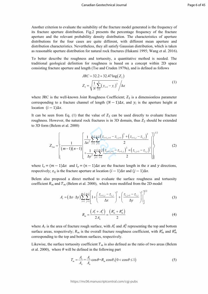
To better describe the roughness and tortuosity, a quantitative method is needed. The traditional geological definition for roughness is based on a concept within 2D space consisting fracture aperture and length (Tse and Cruden 1979a), and is defined as follows

2

22 1

1

32.2 32.47log

1 N

i ii

JRC Z

Z y y xN

(1)

where JRC is the well-known Joint Roughness Coefficient; is a dimensionless parameter 𝑍2

corresponding to a fracture channel of length , and is the aperture height at (𝑁 ― 1)∆𝑥 𝑦𝑖

location .(𝑖 ― 1)∆𝑥

It can be seen from Eq. (1) that the value of can be used directly to evaluate fracture 𝑍2roughness. However, the natural rock fractures is in 3D domain, thus should be extended 𝑍2to 3D form (Belem et al. 2000)

1 22 21 1

1, 1 , 1 1, ,2

1 12 2 2

1 11, 1 1, , 1 ,

2j 1 1

121

1 1 1+2

m ni j i j i j i j

i jm

n mi j i j i j i j

i

z z z zx

Zm n z z z z

y

(2)

where and are the fracture length in the and directions, 𝑙𝑥 = (𝑚 ― 1)∆𝑥 𝑙𝑦 = (𝑛 ― 1)∆𝑥 𝑥 𝑦respectively; is the fracture aperture at location and .𝑧𝑖𝑗 (𝑖 ― 1)∆𝑥 (𝑗 ― 1)∆𝑥

Belem also proposed a direct method to evaluate the surface roughness and tortuosity coefficient and (Belem et al. 2000), which were modified from the 2D model𝑅𝑚 𝑇𝑚

1 22 21 1

1, , , 1 ,

1 11

m ni j i j i j i j

ri j

z z z zA x y

x y

(3)

2 2

t b t br r m m

mn

A A R RR

A

(4)

where is the area of fracture rough surface, with and representing the top and bottom 𝐴𝑟 𝐴𝑡𝑟 𝐴𝑏

𝑟

surface areas, respectively; is the overall fracture roughness coefficient, with and 𝑅𝑚 𝑅𝑡𝑚 𝑅𝑏

𝑚corresponding to the top and bottom surfaces, respectively.

Likewise, the surface tortuosity coefficient is also defined as the ratio of two areas (Belem 𝑇𝑚

et al. 2000), where will be defined in the following part𝜃

= cos = cos , 0 cos 1r rm m

n

A AT RA A

(5)

Page 6 of 45



Draft

where, is the area of the best fitting surface that can pass through the four extreme points 𝐴𝜋of the rough surface, called “π-surface”, which is defined as

0x y z (6)

The coordinates of the four points can be substituted into Eq. (6), then the value of and 𝛼 𝛽can be calculated based on the least square regression method. Then, can be derived, as 𝑇𝑚

can be expressed as follows,cos𝜃

2 2cos =1 + +1 (7)

If the “π-surfaces” of the top and bottom surfaces are different, the overall surface tortuosity coefficient of a rough fracture is calculated as,

cos cos= =2cos coscos cos

t b t b t br r r r

m mt b t bt bn n

A A A AT RA A A A

(8)

As for the mean mechanical aperture of a 3D fracture, it can be defined as follows

, ,1 1

1 m nt b

m i j i ji j

h z zmn

(9)

where, and are the points located at the top and bottom surfaces with coordinates of 𝑧𝑡𝑖,𝑗 𝑧𝑏

𝑖,𝑗

and , respectively.(𝑖 ― 1)∆𝑥 (𝑗 ― 1)∆𝑦

Therefore, the characteristics of four cases presented in Fig.1 can be quantified, and the results are listed in Table 1. As discussed above, there are differences among different cases in Fig.1, whereas Table 2 describes the differences more directly and accurately. Meanwhile, it can be found that the values of and are extremely close to each other, due to the fact 𝑅𝑚 𝑇𝑚

that the tortuosity of rock fractures studied here are very low, which can lead to small (close 𝜃to 0) and large (close to 1), so we have according to Eq. (5) .cos𝜃 𝑇𝑚 ≈ 𝑅𝑚 𝑇𝑚 = 𝑅𝑚cos𝜃

Then the characteristic parameters of all rock fractures, generated according to parameters given in Table A1-1 (in Appendix A1), can be described based on Eqs. (2) to (9), and the results are presented in Table A1-2 (in Appendix A1), including the mean mechanical aperture , dimensionless parameter , the fracture roughness and tortuosity and . ℎ𝑚 𝑍2𝑚 𝑅𝑚 𝑇𝑚As shown in Fig. A1-1 in Appendix A1, the bar diagrams in the diagonal are parameter distributions of , , and , respectively, and the rest sub-diagrams show correlations 𝑍2𝑚 𝑅𝑚 𝑇𝑚between any two specific parameters. It can be easily found that the distributions of three parameters are quite similar; and the relationship between and ( ) is approximately 𝑍2𝑚 𝑅𝑚 𝑇𝑚

linear, whereas and is linearly correlated.𝑅𝑚 𝑇𝑚

3 Fluid transportation through rough fractures

To study the characteristics of fluid flow through rough rock fractures, including the relationship between inlet flow rate and inlet pressure, the pressure or velocity distribution, and the equivalent fracture aperture, simulations of Newtonian flow through rough rock fracture are conducted based on the Navier-Stokes Equations. The simulation model is shown in Fig.3, where all four models have the same boundary conditions: there is no outflow from lateral boundaries on two sides along the flow direction; the top and bottom rough surfaces are assumed to be impermeable and the coupling effect between fluid flow and rock fracture is not considered here.

Page 7 of 45



Draft

A constant inlet flow rate is assumed as the boundary condition at the inlet end, and the mass flow rate applied is 0.1 to 0.7 kg/s, corresponding to 6 to 35 L/min; the pressure is assumed to be zero at the outlet end. Two cuboids are attached to the left and right ends of the fracture model, which are used to reduce the boundary influence, and to make it easier to get convergent solution. The size of the two cuboids is designed in such a way so that the cross section of rock fracture at both ends can be included inside the corresponding cuboids surfaces, as can be seen from Figs. 3 and 4. Normally, their sizes are the same within one fracture model, and they vary among different fracture models.

Take Case 1 as an example, the velocity distribution inside the rock fracture is shown in Fig.4, where velocity distribution in five longitudinal cross-sections (five slices) are presented, and the red and blue colours refer to high and low velocities, respectively. As it can be seen from Fig.4, the inlet velocity at the cuboid is stable and uniform, indicating its function for stabilising the inlet flow into the rough rock fracture.

One important observation is that bright red colour concentrates mainly at the middle of the fracture, defined as central areas (CA); and the colour close to the fracture wall is dark blue (extremely small velocity), defined as surface concave areas (SCA), especially at the location with large concaves, indicating that these areas do not effectively contribute to the transportation of fluid. The same phenomena can be found for all other cases. Therefore, we can conclude that only part of the rough rock fracture is effective for fluid transportation and propose the “equivalent hydraulic aperture (EHA)” for evaluation of this phenomenon.

To investigate the general situation, we also conducted numerical simulation using Bingham model, the simulation results of which are compared with that under Newtonian model, including the corresponding inlet pressure generated, and the velocity fields. One example is presented in detail in Fig. A2-1 (see Appendix A2). It is observed that the differences of simulation results between the two models are very small, under the same constant inlet flow rates, except that the relevant computational efficiency of Newtonian flow is far higher.

4 Evaluation and prediction of EHA

4.1 Theoretical equation and EHA evaluation

As for water flowing between two rough surfaces, three parameters can be used for describing the fluid field: flow rate , pressure gradient , and hydraulic aperture , and their 𝑄𝑚 ∆𝑃 ℎ𝑒relationship can be expressed as (Thompson 1991)

1 312 m

eQh

W P

(10)

where, and are the viscosity and density of Newtonian flow, respectively; and are the 𝜇 𝜌 𝑊 𝐿width and length of the fracture channel, respectively. Then the rough fracture is equivalent to a fracture channel with two smooth parallel surfaces, as shown in Fig. 5.

As shown in Fig.5, the average pressures at two cross sections in plane at y=0 and 100 𝑥𝑧(mm) are taken as and 0 respectively, then the pressure gradient in Eq. (10) is . 𝑃0 ∇𝑃 = 𝑃0 𝐿

In generalization, Newtonian flow is a special case of Bingham flow when the corresponding yield stress is taken as zero. Furthermore, for grouting of rock fractures, cement grout with water cement ratio (W/C) around 1 is usually used (Warner 2004), which can be taken as Bingham flow (Rosquoët et al. 2003; Ruan 2005). For Bingham flow, the corresponding EHA can also be deduced from analysis of the corresponding flow rate expression (Xiao et al. 2017)

Case 3

Case 4

Case 1

Page 8 of 45



Draft

33

0 00 0= 1 3 4 ,

12e

me e

Wh y yPQ y P xx h h

(11)

where, is the yield stress of Bingham flow; is the pressure gradient, and it is 𝜏0 ― ∂𝑃 ∂𝑥taken as , thus the half width of the Bingham plug is . Eq. (11) is derived by 𝑃0 𝐿 𝑦0

𝜏0𝐿 𝑃0assuming that grout flows within parallel plates with a distance of .ℎ𝑒

The relationship between and is nonlinear, so we cannot express as a function of 𝑄𝑚 ℎ𝑒 ℎ𝑒 𝑄𝑚directly. Thus, some transformations should be introduced to determine indirectly.ℎ𝑒

Here, we introduce a dimensionless variable . Then, substitute into Eq. (11)∅ = 𝑦0 ℎ𝑒 ∅

2 30 0

3

1 3 4=12mW yQ

(12)

Rewrite Eq. (12) as cubic equation of as follows,∅

30 4 3 1 0C (13)

where, is a dimensionless constant under specific inlet flow rate. We 𝐶0 = 12𝜇𝑄𝑚 𝜌𝑊𝜏0𝑦20

can rewrite to find the corresponding physical meaning,𝐶0

2

0 00 02 2

0 0 0 0 0

12 12= ,m mQ Q PC yW y WL P L

For a given rock fracture ( and are fixed), inlet flow rate ( is fixed), and Bingham flow 𝑊 𝐿 𝑄𝑚

( and are fixed), the first two terms inside brackets are constants, so is positively 𝜇 𝜏0 𝐶0

proportional to square of the ratio of inlet pressure to yield stress, namely . 𝐶0 ∝ (𝑃0 𝜏0)2

Therefore, for the same , the value of increase with decreasing , indicating that the 𝑃0 𝐶0 𝜏0

fluid increasingly resembles Newtonian fluid, which will be validated in the following discussions. Therefore, we define as the index of Newtonian flow (INF), indicating the 𝐶0degree of similarity between a Bingham flow and a Newtonian flow rises with increasing INF.

For a special situation with ( ), the EHA can be expressed as a simple function ∅ = 1 3 𝐶0 = 4of the inlet pressure

0 0 03 3eh y L P (14)

Here, Eq. (14) can be used to calculate the EHA when the relationship between the inlet flow rate and pressure is . It could be very useful for conducting laboratory 𝑄𝑚 = 𝜌𝑊𝐿2𝜏2

0 3𝜇𝑃20

testing using Bingham fluid, when the test setup satisfies this condition.

Let , and when , then Eq. (13) becomesλ1 = 3 (𝐶0 ― 4) λ2 = ― 1 (𝐶0 ― 4) 𝐶0 ≠ 4

31 2 0 (15)

To solve the cubic equation, firstly, we should determine the discriminant of Eq. (15),∆

2 3002 1

300

0, 40, 42 3 4 4

if CCif CC

Page 9 of 45



Draft

There is only one real root of Eq. (15) that satisfies , as the other two roots are 𝐶0 > 4imaginary numbers, thus the unique solution of Eq. (15) is

3 32 22 2 (16)

For typical grouting projects, is normally a very large number, therefore, Eq. (13) can be 𝐶0

simplified as , then , , and . Finally, we 𝐶0∅3 +3∅ ― 1 = 0 λ1 = 3 𝐶0 λ2 = ― 1 𝐶0 ∆ = 1 4𝐶20

have , so the EHA is , which is the same as ∅ = 𝐶 ―1 30 h𝑒 = 𝐶1 3

0 𝜏0𝐿 𝑃0 = (12𝜇𝑄𝑚𝐿 𝜌𝑊𝑃0)1 3

that given in Eq. (10) for Newtonian flow.

In some laboratory tests, the inlet flow rate or pressure might be very low, so the condition 𝐶0

might occur. In that case, there would be three real roots for Eq. (15)< 4

1 1

2 1

3 1

=2 3 cos 3

2 3 cos 2 3

2 3 cos 2 3

(17)

where, , thus . 𝛼 = cos ―1 [ ―1 2 (4 ― 𝐶0)5] α ∈ [𝜋 2,𝜋]

As , the range of angle in Eq. (17) can be estimated as, α ∈ [𝜋 2,𝜋] ∅

2

1 3

3 6, 30

2 3 5 3,0

2 3 2, 3

As for the negative solution, should not be accepted as a useful solution, as should be ∅2 ∅positive to ensure that the relevant pressure drop per unit length . In the 𝑃0 𝐿 = 𝜏0 (∅ℎ𝑒) > 0meanwhile, consider the expression of pressure drop , the conditions 𝑃0 𝐿 = 𝜏0 (∅ℎ𝑒) ∅1 > ∅3

indicate that the relevant inlet pressure corresponding to is higher than for the > 0 ∅3 ∅1same fracture. If a lower pressure can make the cement grout move with a flow rate of , a 𝑄𝑚

higher pressure can lead to higher flow rate. Thus, is taken as the root of Eq. (15) ∅1

21 00 0 0

50 0 00

=2 1 4 cos 3 12=arccos 1 2 4

mC C Q W y

y L PC

(18)

Then, the EHA can be calculated as , according to Eq. (18). ℎ𝑒 = 𝑦0 ∅1

A summary is presented in Table 2 for calculation of EHA under different situations. In grouting practice, the dimensionless parameter is normally far larger 𝐶0 = 12𝜇𝑄𝑚 𝜌𝑊𝜏0𝑦2

0than 4, then Eq. (16) degenerate into Eq. (10) when used for calculating the EHA for Bingham fluid, which is beneficial to engineering practice.

All 58 different rough fracture models generated in Section 2 are used for numerical simulation, similar to those conducted in Section 3, where the fluid type used is Newtonian flow, and the corresponding inlet flow rate ranges from 0.1 to 0.7 kg/s within an interval of 0.1 kg/s. The inlet pressure from all numerical simulations are recorded, then the 𝑃0corresponding is calculated according to Eq. (10). The simulation results and the EHAs ℎ𝑒calculated are presented in Table A1-3 (see Appendix A1). It can be found that the EHA

Page 10 of 45



Draft

decreases with increasing mass flow rate, directly indicating that the effective aperture for fluid transportation is shrinking with an increasing flow rate. In fact, it can be seen from Eq.

(10) that would decrease with increasing only when the ℎ𝑒 = (12𝜇𝑄𝑚𝐿 𝜌𝑊𝑃0)1 3𝑄𝑚

corresponding inlet pressure is of higher rate of rise than that of , indicating that the 𝑃0 𝑄𝑚energy lost increase faster than its supply from some energy sources, like injection pump. This phenomenon exists for fluid flow within both rough fractures and smooth fractures, which can be seen from Fig. 6, where the ratios of (the unit of this ratio is ignored) for 𝑄𝑚 𝑃058 cases are presented, and the mean mechanical apertures of rough fractures listed Table A1-2 (see Appendix A1) are taken as the apertures of all smooth fractures correspondingly.

As can be seen from Fig. 6, for both smooth and rough fractures, the ratio is declining 𝑄𝑚 𝑃0with increasing inlet flow rate , whereas the rate of declining for rough fractures is faster 𝑄𝑚than that for smooth fractures, indicating that the existence of surface roughness and tortuosity can lead to higher and faster energy lost.

4.2 Development of surrogate model for EHA prediction

It would be of great significance if we can build a surrogate model for predicting the EHA of rough rock fractures just based on some readily available geological data, without knowing details of fracture surfaces, as the concept of EHA is important not only to the field of hydraulics but also to other areas. Again, field grouting, for instance, it would be very useful if we can know in advance the injection pressure corresponding to a specific injection flow rate, as the injection pressure can be used to evaluate the potential fracture (or rock mass) deformation, which is critical to the stability and safety of tunnel or rock cavern under excavation. It is known that the characteristic parameters of rock fractures can be evaluated from geological data, and the potential injection flow rate can be read and determined from the grouting pump, which are all data that can be used to predict the injection pressure. Through data analysis, we found that a predictive model of high accuracy, for predicting the EHA of a fracture, can be built utilizing only geological data and the correlated injection rate based on Artificial Neural Network (ANN), and more details will be introduced in the following sections.

Therefore, we can indirectly calculate the injection pressure of a specific rough rock fracture via transformed Eq. (10),

0 3

12 m

e

Q LPWh

(19)

The process for building an ANN based predictive model and evaluating injection pressure is presented in a schematic diagram in Fig.7, where, , FD, and AF are standard deviation, σ𝑚fractal dimension, and anisotropy factor of rock fractures.

The ANN based predicative model is developed using data from Tables A1-1, A1-2, and A1-3 (see Appendix A1), which can be adopted to calculate the injection pressure under given injection rate and geological conditions (characteristics of rough rock fractures).

4.2.1 ANN based model

Data mining is usually based on intelligent algorithms, among which ANN is very popular, whose original goal was to solve problems in the same way that a human brain would (Hagan et al. 1996). So far, ANNs have been used in many areas, such as computer vision, speech recognition, machine translation, social network filtering, playing board and video games and medical diagnosis (Acharya et al. 2003; Brause et al. 1999; Evangelou et al. 2001; Kim and

Page 11 of 45



Draft

Han 2000; Patil and Kumaraswamy 2009). In the field of civil engineering, there are also many applications, geological data was used for developing predictive model for dynamically evaluating engineering parameters, such as ground settlement, grout penetration range, where the relationship between geological data and parameters to be evaluated are highly nonlinear but the results obtained in literature were good (Li et al. 2017; Suwansawat and Einstein 2006; Zhong et al. 2015). The schematic diagram of ANN used in the present work is shown in Fig.7, where there are 8 nodes in the input layer, 6 hidden nodes in the hidden layer, and 1 output node in the output layer. The detailed algorithm and principles behind neural network will not be presented here, as it has been introduced in many papers (Hagan et al. 1996; Mahdevari and Torabi 2012; Suwansawat and Einstein 2006; Zurada 1992).

One sample is defined as a rough rock fracture under one inlet flow rate. In total, there are 58 rough rock fractures and 7 types of inlet flow rate, so the total sample size equals 58*7=406. All samples are used for developing the ANN based predictive model, and they were divided randomly into three parts: training set (70%, 284 samples), validation set (15%, 64 samples), and test set (15%, 64 samples), where the training and validation sets work together to build a predictive model, whereas the test set is for estimating the performance of the model trained. The performance of the predictive model developed is shown in Fig.8, where the coefficient of correlation (R) for three data sets and all data are evaluated, and its definition is as follows

1 1 2 21 2 1

2 21 21 1 2 2

1 1

,

var var

n

k kk

n n

k kk k

x x x xCov x xR

x x x x x x

(20)

where and are two variables, and, in the present work, they represent target and output, 𝑥1 𝑥2respectively; is the covariance of two variables; and 𝐶𝑜𝑣(𝑥1,𝑥2) 𝑣𝑎𝑟(𝑥1) 𝑣𝑎𝑟(𝑥2)represent standard deviation of two variables, respectively; and are mean values of two 𝑥1 𝑥2variables; is the number of components in two variables; and are the kth 𝑛 𝑥𝑘1 𝑥𝑘2components of two variables, respectively.

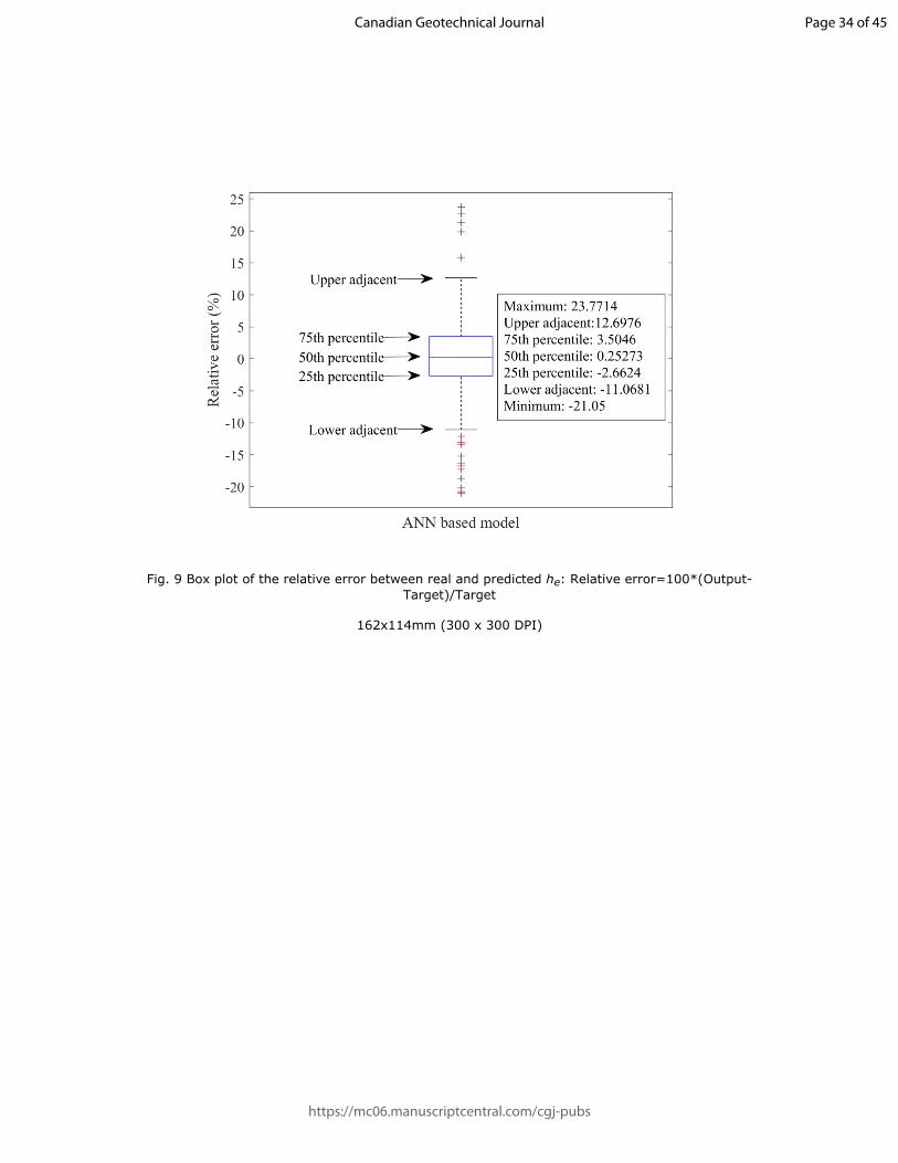
R is usually used for measuring how strong one variable is correlated to another variable, and R=1 indicates a strong positive relationship. As can be seen from Fig. 8, all the R involved are close to 1, indicating that the target (practical ) can be well described by the output ℎ𝑒(predicted ). To examine the degree of accuracy of the predictive model, the distribution of ℎ𝑒relative error between real and predicted is shown in Fig.9 using box plot, where the ℎ𝑒relative error between 12.6976% and -11.0681% accounts for 96.06% of all sample points, among which only 16 are outliers (shown as “+”). Here, define two variables: UA (upper adjacent) and LA (lower adjacent), with and LUA = 𝑞3 +𝑤(𝑞3 ― 𝑞1) = 12.6976 A = 𝑞1 ―𝑤

, where is the maximum whisker length of default value 1.5; (𝑞3 ― 𝑞1) = ―11.0681 𝑤 𝑞3 and are the 75th and 25th percentiles, respectively. A percentile is = 3.5046 𝑞1 = ―2.6624

the value less than which a given percentage of sample points in a set of sample points fall. The outliers are those points with relative error larger than UA and less than LA.

It can be found from the above discussions that the EHA can be well described by the ANN based predictive model utilizing only geological data and the corresponding inlet rate. In other words, the EHA is a function of geological data and inlet rate, whereas the function behind the ANN algorithm is too complex, it is hard to derive an expression for the function with obvious physical meaning. Therefore, in the following discussion, we will manage to derive a simple expression for the EHA.

4.2.2 Regression based model

Page 12 of 45



Draft

As discussed in Section 4.2.1, the EHA is a function of both the inlet flow rate and the ℎ𝑒characteristics of rough rock fracture, including its roughness , tortuosity , mean 𝑅𝑚 𝑇𝑚mechanical aperture , the fractal dimension, standard deviation , and so on. To derive a ℎ𝑚 𝜎𝑚simple form expression, all the data should be analysed and pre-processed. Firstly, there are seven inlet rates, and every time all fractures (generated according to Table A1-1 in Appendix A1) is under only one inlet rate, so is taken as a special factor. As for the remaining seven 𝑄𝑚parameters, it is important to evaluate the importance of each factor and reduce the number of input parameters required. After step-by-step analysis, it is found that the relationship between and , , and can be expressed by a linear polynomial, the coefficients of ℎ𝑒 𝜎𝑚 𝑅𝑚 ℎ𝑚

which are linear function of . 𝑄𝑚

From stepwise regression analysis based on MATLAB programming, it is found that fracture roughness , standard deviation of fracture aperture , and the mean mechanical aperture 𝑅𝑚 𝜎𝑚

are the three most important impact factors to the EHA under one inlet rate. The fractal ℎ𝑚dimension and anisotropy factor are not considered separately, since there is causal relationship between them and the remaining factors. Meanwhile, among , and , 𝑍2𝑚 𝑅𝑚 𝑇𝑚only is taken as the most critical factors, since the magnitude and variation trends of these 𝑅𝑚three parameters are more or less the same, as discussed in Section 2, so it is reasonable to assume that alone can represent their overall impact. The mean mechanical aperture 𝑅𝑚 ℎ𝑚and its standard deviation describe the magnitude and the degree of concentration of 𝜎𝑚fracture aperture, respectively, so they are bound to be among the most critical factors.

In building a prediction model correlating EHA to the fracture roughness , the standard ℎ𝑒 𝑅𝑚deviation of fracture aperture , and the mean mechanical aperture , an explicit 𝜎𝑚 ℎ𝑚

expression in a polynomial form is used, i.e. , where , ℎ𝑒 = ∑𝑁𝑛 = 0(𝑏𝑛𝑅𝑖

𝑚ℎ𝑗𝑚𝜎𝑘

𝑚) 𝑖 ∈ [0,𝑚1] 𝑗 ∈, and , is the number of polynomial terms; , , and are the [0,𝑚2] 𝑘 ∈ [0,𝑚3] 𝑁 𝑚1 𝑚2 𝑚3

maximum exponents corresponding to , , and , respectively; and a constant term 𝑅𝑚 𝜎𝑚 ℎ𝑚

exists when . The EHA obtained thus far is under a specific inlet flow rate, 𝑖 = 𝑗 = 𝑘 = 0 ℎ𝑒and it may vary under different inlet flow rates, so we need to establish the relationship between inlet flow rates and the coefficients , expressed as . 𝑄𝑚 𝑏𝑛 𝑏𝑛 = 𝑓𝑛(𝑄𝑚),(𝑛 ∈ [0,𝑁])Then, EHA can be expressed as . Finally, the EHA expression ℎ𝑒 = ∑𝑁

𝑛 = 0[𝑏𝑛(𝑄𝑚)𝑅𝑖𝑚ℎ𝑗

𝑚𝜎𝑘𝑚]

should be validated with extra cases. The detailed process for deriving the prediction model is described in the following sections.

In the present work, linear regression is tried first

0

N

e i ii

h b b x (21)

where, is number of impact factors, and represent the impact factor and the 𝑁 = 3 𝑥𝑖 𝑏𝑖regression parameters, represents the standard deviation of fracture aperture , 𝑥1 𝜎𝑚 𝑥2represents the fracture roughness , and represents the mean mechanical aperture .𝑅𝑚 𝑥3 ℎ𝑚

The parameter array is obtained when the minimum value of the sum of 𝐵 = [𝑏0,𝑏1,⋯,𝑏𝑁]squared residual error (SSE or RSS) between the predicted and real is reached,ℎ𝑒 ℎ𝑒

2

1

ˆarg minN

e eB i

B h h

(22)

Page 13 of 45



Draft

Then, the predicted EHA can be obtained based on Eq. (21). Statistical distribution of the relative error between real and that predicted by the regression based analytical model is ℎ𝑒present in Fig.10, where the relative error in more than 90% of all cases is within the interval of [-20, 20], and that in more than 65% of all cases is within the interval of [-10, 10], indicating that the regression based analytical model derived is of high accuracy.

The function derived so far is still under some specific inlet rate, so we should integrate the special parameter into the expression in the next step. Hence, plot the parameter array of 𝑄𝑚

in Fig.11, to see the relevant variation patterns. As can be seen, the value of and is 𝐵 𝑏1 𝑏2negative, indicating that the existence of aperture deviation and fracture roughness can reduce the relevant EHA, which is reasonable and acceptable.

Moreover, with increasing , and are increasing, and and are decreasing. 𝑄𝑚 𝑏2 𝑏3 𝑏0 𝑏1Therefore, it is reasonable to express the relevant relationship with linear equation, which is obtained through finding the best fitting lines passing through all the points corresponding to four coefficients, respectively. The linear regression curves are also drawn in Fig.11, where there is very good linear fitting.

The final prediction model, which includes the standard deviation of fracture aperture , 𝜎𝑚fracture roughness , mean mechanical aperture , and flow rate can be expressed as𝑅𝑚 ℎ𝑚 𝑄𝑚

0

0 1 1

2 3 2

3

0.327 0.5

0.311 0.5

0.144 0.232

0.546 0.761

m m

e m m m m m

m m m m m m

m m

b Q Q

h b Q b Q b Q Q

b Q R b Q h b Q Q

b Q Q

(23)

Eq. (23) are used to calculate the EHAs of all cases under grout inlet rate of 0.1, 0.6, and 0.7 kg/s, respectively. The prediction results are compared with that based on numerical simulations and Eq. (10), as presented in Fig.12. The input parameters for the prediction model are only the characteristics of rock fractures ( , , and ), and the specific grout 𝑅𝑚 ℎ𝑚 𝜎𝑚inlet flow rate . It can be found from Fig. 12 that there are small differences between the 𝑄𝑚EHA predicted by the regression based analytical model and that from numerical simulations for most cases, which verifies that the derived predictive model has a high degree of accuracy, and it can predict the EHA of rock fracture under a specific inlet flow rate.

The accuracy of the prediction model for the cases under inlet flow rate is 𝑄𝑚 = 0.7𝑘𝑔/𝑠slightly lower than that under and , since the latter two inlet 𝑄𝑚 = 0.1𝑘𝑔/𝑠 𝑄𝑚 = 0.6𝑘𝑔/𝑠flow rates are closer to the flow rate interval [0.2, 0.5] (kg/s) used for model training. This indicates that a wider range of data used for training can lead to a better prediction model, i.e., with higher accuracy.

5 Potential application

Under the condition that Eq. (23) is obtained through a large number of training cases, the coefficients and should be reliable to be used in , 𝑎𝑖0 𝑎𝑖1 𝑏𝑖(𝑄𝑚) = 𝑎𝑖1𝑄𝑚 + 𝑎𝑖0,(𝑖 = 0,1,2,3)which can be used to predict the EHAs using onsite data, then other characteristics of rock fractures can be calculated based on the EHA obtained, finally we can utilize all information derived to estimate the volume of grout in need. Moreover, the ANN based predictive model can also be used here to calculate the corresponding .ℎ𝑒

Consider an isolated fracture in rock mass, of which both the width and length are unknown, but some geological data can be obtained via site investigation. A simplified schematic

Page 14 of 45



Draft

diagram of a designed experiment is shown in Fig.13, where the rock fracture is assumed to be a rectangular with finite width and length. The pressure measured from holes H1 and H2 (when the flow is stable) can be used for calculating the pressure difference between two holes, which is taken as the nominal inlet pressure; meanwhile, the steady flow rate of outflow water from hole H2 is recorded. The top and bottom surfaces are rough but are not illustrated here.

The basic information concerning the characteristics of rock fractures, including the mean mechanical aperture , the fracture roughness , and its standard deviation , can be ℎ𝑚 𝑅𝑚 𝜎𝑚estimated according to data analysis of the rock samples from early site investigation. The distance between the two holes is L = 5m, which can be taken as the nominal fracture length. The fracture width W is the unknown parameter, but it is a critical parameter for grouting design, as the void volume of the rock fracture can be calculated as , 𝑉𝑓𝑟𝑎𝑐 𝑉𝑓𝑟𝑎𝑐 = 𝑊𝐿ℎ𝑚which is the volume of grout required for filling the fracture. However, the width W can be calculated through the following equation transformed from Eq. (10)

30

12 m

e

Q LWP h

(24)

In Eq. (24), the EHA can be calculated based on Eq. (23) utilizing the site data. As shown in Table 3, three sets of data from the designed experiment are used to derive three pairs of 𝑃𝑖

0

and (i=1,2,3) for better estimation of fracture width W. 𝑄𝑖𝑚

Substitute the water flow rate (i=1,2,3), and the characteristic information of rock 𝑄𝑖𝑚

fractures into Eq. (23), we have three EHAs (i=1,2,3)ℎ𝑖𝑒

1 1 1 1 10 1 2 3

2 2 2 2 20 1 2 3

3 3 3 3 30 1 2 3

m m m m m m m e

m m m m m m m e

m m m m m m m e

b Q b Q b Q R b Q h h



(25)

where, the coefficients and for expression , (i=1,2,3; j=0,1,2,3) 𝑎𝑖0 𝑎𝑖1 𝑏𝑗(𝑄𝑖𝑚) = 𝑎𝑗1𝑄𝑖

𝑚 + 𝑎𝑗0

is the same as that presented in Eq. (23).

By using the EHA obtained from Eq. (25), the fracture width W via Eq. (24) can be ℎ𝑒calculated, which are presented in Table 4, where three fracture widths calculated are very close to each other, indicating good prediction accuracy and the feasibility of the proposed potential application.

Thereafter, the volume of the cement grout required for sealing this fracture is taken as

3 32.145frac mV W L h e m

6 Conclusions

In the present work, a model was developed to generate synthetic rough surfaces of rock fractures, and the fracture characteristics were analysed based on a MATLAB program. A numerical model for fluid transportation simulation based on the proposed rock fractures was also developed, and the simulation results were used for demonstrating and calculating the concept and value of equivalent hydraulic aperture (EHA) of rock fractures, respectively. Two aperture prediction models were built based on the simulation data using different methods. A designed experiment was introduced to demonstrate the potential application of the proposed predictive model for grouting design. The fluid type used for numerical simulation is

Page 15 of 45



Draft

Newtonian flow, which is a special case of Bingham flow, so three equations were derived for calculating EHA corresponding to Bingham flow under different conditions.

The following conclusions can be obtained:

1. Larger mean mechanical aperture of a rough rock fracture is correlated with higher fracture roughness and tortuosity.

2. Compared with ideal fracture channel with the same mean mechanical aperture, effective spaces for fluid transportation in rough rock fracture are considerably reduced due to the existence of surface concave areas, which can be quantitatively evaluated by EHA.

3. With the increase of inlet flow rate, the inlet pressure is increasing, but the corresponding EHA is decreasing, probably because the corresponding energy lost increases faster than the corresponding increase rate of energy supply.

4. The EHA can be calculated based on a predictive model consisting of grout inlet flow rate, standard deviation and mean mechanical aperture of rock fracture, and fracture roughness, and it is negatively related to the standard deviation and roughness of a rock fracture.

5. The concept of EHA has feasibility and potential in practical application.

Reference

Acharya, U.R., Bhat, P.S., Iyengar, S.S., Rao, A., and Dua, S. 2003. Classification of heart rate data using artificial neural network and fuzzy equivalence relation. Pattern recognition 36(1): 61-68. doi: 10.1016/S0031-3203(02)00063-8.

Amadei, B., and Illangasekare, T. 1994. A mathematical model for flow and solute transport in non-homogeneous rock fractures. International Journal of Rock Mechanics and Mining Sciences & Geomechanics Abstracts 31(6): 719-731. doi: 10.1016/0148-9062(94)90011-6.

Belem, T., Homand-Etienne, F., and Souley, M. 2000. Quantitative parameters for rock joint surface roughness. Rock mechanics and rock engineering 33(4): 217-242. doi: 10.1007/s006030070001.

Brause, R., Langsdorf, T., and Hepp, M. 1999. Neural data mining for credit card fraud detection. In Tools with Artificial Intelligence, 1999. Proceedings. 11th IEEE International Conference on. IEEE. pp. 103-106.

Briggs, S., Karney, B.W., and Sleep, B.E. 2014. Numerical modelling of flow and transport in rough fractures. Journal of Rock Mechanics and Geotechnical Engineering 6(6): 535-545. doi: 10.1016/j.jrmge.2014.10.004.

Briggs, S.A. 2014. Impact of Single Fracture Roughness on the Flow, Transport and Development of Biofilms. University of Toronto, Toronto.

Brown, S.R. 1987. Fluid flow through rock joints: the effect of surface roughness. Journal of Geophysical Research: Solid Earth 92(B2): 1337-1347. doi: 10.1029/JB092iB02p01337.

Brush, D.J. 2001. Three-dimensional fluid flow and solute transport in rough-walled fractures. University of Waterloo, Ontario.

Brush, D.J., and Thomson, N.R. 2003. Fluid flow in synthetic rough‐walled fractures: Navier‐Stokes, Stokes, and local cubic law simulations. Water Resources Research 39(4). doi: 10.1029/2002WR001346

Page 16 of 45



Draft

Chen, C.Y., and Horne, R.N. 2006. Two‐phase flow in rough‐walled fractures: Experiments and a flow structure model. Water resources research 42(3). doi: 10.1029/2004WR003837

Crandall, D., Bromhal, G., and Karpyn, Z.T. 2010. Numerical simulations examining the relationship between wall-roughness and fluid flow in rock fractures. International Journal of Rock Mechanics and Mining Sciences 47(5): 784-796. doi: 10.1016/j.ijrmms.2010.03.015.

Develi, K., and Babadagli, T. 2015. Experimental and visual analysis of single-phase flow through rough fracture replicas. International Journal of Rock Mechanics and Mining Sciences 73: 139-155. doi: 10.1016/j.ijrmms.2014.11.002.

El Tani, M. 2012. Grouting Rock Fractures with Cement Grout. Rock Mechanics and Rock Engineering 45(4): 547-561. doi: 10.1007/s00603-012-0235-0.

Emmelin, A., Brantberger, M., Eriksson, M., and Gustafson, G. 2007. Rock grouting. Current competence and development for the final repository. Swedish Nuclear Fuel and Waste Management Co., Stockholm (Sweden).

Eriksson, M., Stille, H., and Andersson, J. 2000. Numerical calculations for prediction of grout spread with account for filtration and varying aperture. Tunnelling and Underground Space Technology 15(4): 353-364. doi: 10.1016/S0886-7798(01)00004-9.

Evangelou, I.E., Hadjimitsis, D.G., Lazakidou, A.A., and Clayton, C. 2001. Data mining and knowledge discovery in complex image data using artificial neural networks. In in Proc. Workshop Complex Reason. Geogr. Data, Paphos. Citeseer.

Fransson, Å., Tsang, C.F., Rutqvist, J., and Gustafson, G. 2010. Estimation of deformation and stiffness of fractures close to tunnels using data from single-hole hydraulic testing and grouting. International Journal of Rock Mechanics and Mining Sciences 47(6): 887-893. doi: 10.1016/j.ijrmms.2010.05.007.

Ge, S. 1997. A governing equation for fluid flow in rough fractures. Water Resources Research 33(1): 53-61. doi: 10.1029/96WR02588.

Gothäll, R., and Stille, H. 2010. Fracture–fracture interaction during grouting. Tunnelling and Underground Space Technology 25(3): 199-204. doi: 10.1016/j.tust.2009.11.003.

Hagan, M.T., Demuth, H.B., and Beale, M.H. 1996. Neural network design. Pws Pub. Boston.

Hakami, E. 1995. Aperture distribution of rock fractures.

Hanssen, A.R. 2013. Numerical modelling of Bingham fluid flow and particle transport in a rough-walled fracture. Norwegian University of Science and Technology, Trondheim.

Hernqvist, L., Fransson, Å., and Vidstrand, P. 2008. Numerical modelling of grout spread and leakage into a tunnel in hard rock–A case study. In World tunnel Congress. pp. 482-491.

Hsiung, S.M., Ghosh, A., Ahola, M.P., and Chowdhury, A.H. 1993. Assessment of conventional methodologies for joint roughness coefficient determination. International Journal of Rock Mechanics and Mining Sciences & Geomechanics Abstracts 30(7): 825-829. doi: 10.1016/0148-9062(93)90030-H.

Jeong, W., and Song, J. 2005. Numerical investigations for flow and transport in a rough fracture with a hydromechanical effect. Energy Sources 27(11): 997-1011. doi: 10.1080/00908310490450827.

Kim, K.-j., and Han, I. 2000. Genetic algorithms approach to feature discretization in artificial neural networks for the prediction of stock price index. Expert systems with Applications 19(2): 125-132. doi: 10.1016/S0957-4174(00)00027-0.

Page 17 of 45



Draft

Kvartsberg, S. 2013. On the use of engineering geological information in rock grouting design. Chalmers University of Technology, Göteborg.

Lanaro, F. 2000. A random field model for surface roughness and aperture of rock fractures. International Journal of Rock Mechanics and Mining Sciences 37(8): 1195-1210. doi: 10.1016/S1365-1609(00)00052-6.

Lavrov, A. 2013. Redirection and channelization of power-law fluid flow in a rough-walled fracture. Chemical Engineering Science 99: 81-88. doi: 10.1016/j.ces.2013.05.045.

Li, X., Zhong, D., Ren, B., Fan, G., and Cui, B. 2017. Prediction of curtain grouting efficiency based on ANFIS. Bulletin of Engineering Geology and the Environment: 1-29. doi: 10.1007/s10064-017-1039-y.

Lipscomb, G.G., and Denn, M.M. 1984. Flow of bingham fluids in complex geometries. Journal of Non-Newtonian Fluid Mechanics 14(0): 337-346. doi: 10.1016/0377-0257(84)80052-X.

Lombardi, G. 2002. Grouting of rock masses. In Grouting and ground treatment. ASCE. pp. 164-197.

Mahdevari, S., and Torabi, S.R. 2012. Prediction of tunnel convergence using artificial neural networks. Tunnelling and Underground Space Technology 28: 218-228. doi: 10.1016/j.tust.2011.11.002.

Mandelbrot, B.B. 1985. Self-affine fractals and fractal dimension. Physica scripta 32(4): 257.

Mitsoulis, E. 2007. Flows of viscoplastic materials: models and computations. Rheology reviews 2007: 135-178.

Moon, H.K., and Song, M.K. 1997. Numerical studies of groundwater flow, grouting and solute transport in jointed rock mass. International Journal of Rock Mechanics and Mining Sciences 34(3–4): 206.e201-206.e213. doi: 10.1016/S1365-1609(97)00279-7.

Noiriel, C., Gouze, P., and Madé, B. 2007. Time-resolved 3D characterisation of flow and dissolution patterns in a single rough-walled fracture. J. Krasny and JM Sharp Eds: 629-642.

Odling, N. 1994. Natural fracture profiles, fractal dimension and joint roughness coefficients. Rock mechanics and rock engineering 27(3): 135-153. doi: 10.1007/BF01020307.

Ogilvie, S., Isakov, E., Taylor, C., and Glover, P. 2003. Characterization of rough-walled fractures in crystalline rocks. Geological Society, London, Special Publications 214(1): 125-141. doi: 10.1144/GSL.SP.2003.214.01.08.

Ogilvie, S.R., Isakov, E., and Glover, P.W.J. 2006. Fluid flow through rough fractures in rocks. II: A new matching model for rough rock fractures. Earth and Planetary Science Letters 241(3–4): 454-465. doi: 10.1016/j.epsl.2005.11.041.

Park, C.-K., Keum, D.-K., and Hahn, P.-S. 1995. A stochastic analysis of contaminant transport through a rough-surfaced fracture. Korean Journal of Chemical Engineering 12(4): 428. doi: 10.1007/bf02705806.

Patil, S.B., and Kumaraswamy, Y. 2009. Intelligent and effective heart attack prediction system using data mining and artificial neural network. European Journal of Scientific Research 31(4): 642-656.

Persson, B. 2014. On the fractal dimension of rough surfaces. Tribology Letters 54(1): 99-106. doi: 10.1007/s11249-014-0313-4.

Page 18 of 45



Draft

Power, W.L., and Tullis, T.E. 1991. Euclidean and fractal models for the description of rock surface roughness. Journal of Geophysical Research: Solid Earth 96(B1): 415-424. doi: 10.1029/90JB02107.

Rafi, J.Y., and Stille, H. 2014. Control of rock jacking considering spread of grout and grouting pressure. Tunnelling and Underground Space Technology 40(0): 1-15. doi: 10.1016/j.tust.2013.09.005.

Rafi, J.Y., and Stille, H. 2015. Basic mechanism of elastic jacking and impact of fracture aperture change on grout spread, transmissivity and penetrability. Tunnelling and Underground Space Technology 49(0): 174-187. doi: 10.1016/j.tust.2015.04.002.

Rong, G., Hou, D., Yang, J., Cheng, L., and Zhou, C. 2017. Experimental study of flow characteristics in non-mated rock fractures considering 3D definition of fracture surfaces. Engineering Geology 220: 152-163. doi: 10.1016/j.enggeo.2017.02.005.

Rosquoët, F., Alexis, A., Khelidj, A., and Phelipot, A. 2003. Experimental study of cement grout: Rheological behavior and sedimentation. Cement and Concrete Research 33(5): 713-722. doi: 10.1016/S0008-8846(02)01036-0.

Ruan, W. 2005. Research on diffusion of grouting and basic properties of grouts. Chinese Jounal of Geotechnical Engineering 27(1).

Runslätt, E., and Thörn, J. 2010. Fracture deformation when grouting in hard rock: In situ measurements in tunnels under Gothenburg and Hallandsås. Chalmers University of Technology, Göteborg.

Saeidi, O., Stille, H., and Torabi, S.R. 2013. Numerical and analytical analyses of the effects of different joint and grout properties on the rock mass groutability. Tunnelling and Underground Space Technology 38(0): 11-25. doi: 10.1016/j.tust.2013.05.005.

Sui, W., Liu, J., Hu, W., Qi, J., and Zhan, K. 2015. Experimental investigation on sealing efficiency of chemical grouting in rock fracture with flowing water. Tunnelling and Underground Space Technology 50: 239-249. doi: 10.1016/j.tust.2015.07.012.

Suwansawat, S., and Einstein, H.H. 2006. Artificial neural networks for predicting the maximum surface settlement caused by EPB shield tunneling. Tunnelling and underground space technology 21(2): 133-150. doi: 10.1016/j.tust.2005.06.007.

Thompson, M.E. 1991. Numerical simulation of solute transport in rough fractures. Journal of Geophysical Research: Solid Earth 96(B3): 4157-4166. doi: 10.1029/90JB02385.

Tsang, Y., and Witherspoon, P.A. 1983. The dependence of fracture mechanical and fluid flow properties on fracture roughness and sample size. Journal of Geophysical Research: Solid Earth 88(B3): 2359-2366. doi: 10.1029/JB088iB03p02359

Tse, R., and Cruden, D. 1979a. Estimating joint roughness coefficients. In Int J Rock Mech Min Sci & Geomech Abstr. Elsevier. pp. 303-307.

Tse, R., and Cruden, D.M. 1979b. Estimating joint roughness coefficients. Int J Rock Mech Min Sci & Geomech Abstr 16(5): 303-307. doi: 10.1016/0148-9062(79)90241-9.

Wang, M., Chen, Y.-F., Ma, G.-W., Zhou, J.-Q., and Zhou, C.-B. 2016. Influence of surface roughness on nonlinear flow behaviors in 3D self-affine rough fractures: Lattice Boltzmann simulations. Advances in Water Resources 96: 373-388. doi: 10.1016/j.advwatres.2016.08.006.

Page 19 of 45



Draft

Warner, J. 2004. Practical handbook of grouting: soil, rock, and structures. John Wiley & Sons.

Xiao, F., and Zhao, Z. 2017. Grout Flow in Fracture Channel Considering Fracture Deformation. In 51st US Rock Mechanics/Geomechanics Symposium. American Rock Mechanics Association.

Xiao, F., Zhao, Z., and Chen, H. 2017. A simplified model for predicting grout flow in fracture channels. Tunnelling and Underground Space Technology 70(Supplement C): 11-18. doi: 10.1016/j.tust.2017.06.024.

Xiao, W., Xia, C., Wei, W., and Bian, Y. 2013. Combined effect of tortuosity and surface roughness on estimation of flow rate through a single rough joint. Journal of Geophysics and Engineering 10(4): 045015. doi: 10.1088/1742-2132/10/4/045015.

Zhang, Z., and Nemcik, J. 2013. Friction Factor of Water Flow Through Rough Rock Fractures. Rock Mechanics and Rock Engineering 46(5): 1125-1134. doi: 10.1007/s00603-012-0328-9.

Zhao, Z., Li, B., and Jiang, Y. 2014. Effects of fracture surface roughness on macroscopic fluid flow and solute transport in fracture networks. Rock mechanics and rock engineering 47(6): 2279. doi: 10.1007/s00603-013-0497-1.

Zhong, D., Yan, F., Li, M., Huang, C., Fan, K., and Tang, J. 2015. A real-time analysis and feedback system for quality control of dam foundation grouting engineering. Rock Mechanics and Rock Engineering 48(5): 1947-1968. doi: 10.1007/s00603-014-0686-6.

Zurada, J.M. 1992. Introduction to artificial neural systems. West St. Paul.

Page 20 of 45



Draft

Figure captions

Figure in the main text

Fig. 1 Four typical synthetic models of rough rock fractures

Fig. 2 Percentage frequency of the aperture of synthetic rock fractures

Fig. 3 Fracture models for simulating Newtonian flow within rough rock fractures

Fig. 4 Velocity distributions (Unit: m/s) presented in five different slices of Newtonian flow within rough rock fracture (Case 1 in Fig. 3)

Fig. 5 Schematic diagram for equivalent channel for rough fracture in Fig. 3 (Thompson 1991)

Fig. 6 Comparison between smooth and rough fractures for varying 𝑄𝑚 𝑃0

Fig. 7 Schematic diagram for an ANN based predictive model and its application for field grouting (for grout flow showing Newtonian characteristics only)

Fig. 8 Correlation coefficient (R) of the predictive model developed based on ANN: Target (T) is the real ; Output (Y) is the predicted ℎ𝑒 ℎ𝑒

Fig. 9 Box plot of the relative error between real and predicted : ℎ𝑒 Relative error = 100 ∗(Output ― Target) Target

Fig. 10 Box plot for the distribution of relative error between real and that calculated based ℎ𝑒on Eq. (21): Relative error = 100 ∗ (Output ― Target) Target

Fig. 11 Linear relationship between parameter and inlet flow rate via fitting𝑏𝑖 𝑄𝑚

Fig. 12 Validation of the prediction model for calculating EHA based on the characteristics of rock fracture and the corresponding inlet flow rate. “Prediction model” is based on Eq. (23), and “Simulation” represents calculation utilizing numerical simulation results and Eq. (10)

Fig. 13 Simplified schematic diagram of a rock fracture with length of 5m and width to be determined using the predictive model following Eq. (23): a designed experiment

Figure in Appendix A1

Fig. A1-1 Correlation between , , and 𝑍2𝑚 𝑅𝑚 𝑇𝑚

Figure in Appendix A2

Fig. A2-1 Comparison of grout flow within two rough surfaces based on Bingham and Newtonian model

Page 21 of 45



Draft

Table 1 Characteristic parameters of four rock fractures shown in Fig. 1

Case NO. (mm)ℎ𝑚 𝑍2𝑚 𝑅𝑚 𝑇𝑚

1 2.14 2.3274 2.3353 2.33512 2.46 2.4110 2.4002 2.40013 3.66 2.2863 2.3035 2.30314 0.63 1.1805 1.4931 1.4931

Page 22 of 45



Draft

Table 2 Equations for calculating EHA

Fluid type of cement grout Equation Number

Bingham flow Eq. (14) ( )𝐶0 = 4

Bingham & Newtonian flow Eq. (16) / (10) ( )𝐶0 > 4

Bingham flow Eq. (18) ( )𝐶0 < 4

Page 23 of 45



Draft

Table 3 Data from thought experiment and the fracture characteristics

Data setsTesting pressure

(Pa)Water volume

(L)Time taken

(min)Fracture

characteristics1 212370 120 10 𝜎𝑚 0.75

2 480353 126 7 𝑅𝑚 1.643 864671 216 9 ℎ𝑚 1.13

Page 24 of 45



Draft

Table 4 Determination of fracture width 𝑊

Data NO. (mm)ℎ𝑒 (m)𝑊 Final (m)𝑊

1 0.53 0.3795

2 0.46 0.3850

3 0.42 0.3746

0.3797

Page 25 of 45



Draft

Fig.1 Four typical synthetic models of rough rock fractures

224x159mm (300 x 300 DPI)

Page 26 of 45



Draft

Fig.2 Percentage frequency of the aperture of synthetic rock fractures

293x205mm (150 x 150 DPI)

Page 27 of 45



Draft

Fig.3 Fracture models for simulating Newtonian flow within rough rock fractures

224x159mm (300 x 300 DPI)

Page 28 of 45



Draft

Fig.4 Velocity distributions (Unit: m/s) presented in five different slices of Newtonian flow within rough rock fracture (Case 1 in Fig. 3)

219x94mm (300 x 300 DPI)

Page 29 of 45



Draft

ℎ𝑒

𝑃 = 𝑃0 𝑃 = 0

Flow direction𝑊

L

Fig. 5 Schematic diagram for equivalent channel for rough fracture in Fig. 3 (Thompson 1991)

Page 30 of 45



Draft

Fig.6 Comparison between smooth and rough fractures under different Qm/P0

148x111mm (300 x 300 DPI)

Page 31 of 45



Draft

Fig. 7 Schematic diagram for an ANN based predictive model and its application for field grouting (for grout flow showing Newtonian characteristics only)

254x190mm (300 x 300 DPI)

Page 32 of 45



Draft

Fig. 8 Correlation coefficient (R) of the predictive model developed based on ANN: Target (T) is the real he; Output (Y) is the predicted he

185x185mm (300 x 300 DPI)

Page 33 of 45



Draft

Fig. 9 Box plot of the relative error between real and predicted he: Relative error=100*(Output-Target)/Target

162x114mm (300 x 300 DPI)

Page 34 of 45



Draft

Fig. 10 Box plot for the distribution of relative error between real he and that calculated based on Eq. (21): Relative error=100*(Output-Target)/Target

162x108mm (300 x 300 DPI)

Page 35 of 45



Draft

Fig.11 Linear relationship between parameter bi and inlet flow rate Qm via fitting

209x164mm (300 x 300 DPI)

Page 36 of 45



Draft

Fig. 12 Validation of the prediction model for calculating EHA based on the characteristics of rock fracture and the corresponding inlet flow rate. “Prediction model” is based on Eq. (23), and “Simulation” represents

calculation utilizing numerical simulation results and Eq. (10)

203x152mm (300 x 300 DPI)

Page 37 of 45



Draft

Water ingress

hole

Water recording

hole

H1 H2

Rock fracture

Plan view

H1 H2

A - A

A A

Top surface

Bottom surface

Fig. 13 Simplified schematic diagram of a rock fracture with length of 5m and width to be determined using the predictive model following Eq. (23): a designed experiment

Page 38 of 45



Draft

Appendix A1

Table A1-1 Orthogonal design table on key parameters for generating fracture model

Case NO. TL ML 𝜎𝑚 FD AF

1 20 7 0.89 2.6 0.962 30 7 0.96 2.65 0.923 80 8 0.75 2.75 0.964 50 4 0.89 2.85 0.985 70 5 0.47 2.8 0.966 50 7 0.47 2.75 1.027 50 3 0.61 2.95 0.948 50 2 0.75 2.65 1.069 30 6 0.68 2.75 1.0610 40 7 0.4 2.85 111 50 9 0.4 2.9 0.9612 80 4 0.47 3 1.0413 70 3 0.96 2.6 0.9814 80 6 0.4 2.7 0.9815 80 9 0.61 2.6 1.0216 40 5 0.89 2.65 1.0817 70 6 0.54 2.65 1.0218 30 5 0.61 2.9 119 80 5 0.54 2.85 0.9220 40 2 0.68 2.6 1.0421 20 2 0.54 2.95 122 50 1 0.68 2.8 123 60 5 0.82 2.6 1.0624 20 3 0.4 2.8 1.0625 10 7 0.82 2.7 0.9426 30 2 0.4 3 1.0227 50 5 0.96 2.7 1.0428 40 4 0.82 2.8 1.0229 20 6 0.61 2.85 1.0430 10 2 0.47 2.9 0.9831 50 8 0.54 2.6 1.0832 90 8 0.61 2.8 0.9233 20 9 0.82 2.75 1.0834 60 7 0.54 2.8 0.9835 70 4 0.4 2.95 1.0836 60 9 0.47 2.95 0.9237 20 1 0.47 2.65 0.9438 10 4 0.61 2.65 0.9639 70 9 0.75 2.7 140 90 4 0.54 2.9 1.0641 10 3 0.54 2.75 1.0442 70 8 0.68 2.85 0.9443 10 1 0.4 2.6 0.9244 20 4 0.68 2.7 0.9245 90 6 0.47 2.6 146 90 5 0.4 2.75 0.9447 30 4 0.75 2.6 0.9448 30 1 0.54 2.7 0.9649 90 9 0.68 2.65 0.9850 60 2 0.61 2.7 1.08

Page 39 of 45



Draft

51 40 8 0.47 2.7 1.0652 90 3 0.89 2.7 1.0253 40 9 0.54 3 0.9454 80 3 0.82 2.65 155 30 3 0.47 2.85 1.0856 70 1 0.4 2.9 0.9657 20 6 0.96 2.7 0.9858 10 7 0.47 2.6 0.94

Notes*: TL - transition length; ML - mismatch wavelength; - standard deviation; FD - 𝜎𝑚fractal dimension; AF - anisotropy factor.

A fractal dimension (FD) is an index for evaluating fractal patterns or sets, utilizing the ratio between the variation in detail to the variation in scale to measure their complexity. Therefore, FD is 0 for points (0D sets); 1 for lines (1D sets having length only); 2 for surfaces (2D sets with length and width); and 3 for volumes (3Dsets with length, width, and height). For common geometries, the theoretical FD is their Euclidean or topological dimension (TD). If the theoretical FD of a set exceeds its TD, then its geometry is fractal.

Ideally, rock fractures are usually represented by two smooth parallel plates, the fractal dimension of which is 2. The surfaces of real rock fractures are rough, but they are still surface not volume, so the corresponding fractal dimension is capped at 3. In general, the fractal dimension of synthetic rough rock fractures should range between 2 and 3. It has been verified that the surface fractal dimension of natural rock fracture ranges from 2 to 2.5 (Ogilvie et al. 2006; Persson 2014; Thompson 1991). However, referring to Ogilvie’s research work, FD ranging from 2.6 to 3 should be used as program input to generate real rock fractures, with the corresponding anisotropy factor varying around 1. Determination of other three parameter ranges also follows the same procedure, ensuring that the rough fractures created are practical and reasonable.

Page 40 of 45



Draft

Table A1-2 Characteristics of fracture model generated (based on data from Table A1)

Case number Mean apertureℎ𝑚

Roughness factor𝑍2𝑚

Roughness𝑅𝑚

Tortuosity𝑇𝑚

1 2.03 1.419 1.656 1.6562 2.68 1.798 1.930 1.9303 3.33 1.907 2.013 2.0134 3.41 2.995 2.872 2.8725 2.18 1.382 1.628 1.6286 2.13 1.195 1.502 1.5027 2.14 2.613 2.561 2.5618 1.13 1.403 1.644 1.6449 2.53 1.730 1.879 1.87910 1.88 1.346 1.602 1.60211 2.29 1.528 1.730 1.73012 2.24 2.239 2.265 2.26513 1.92 1.529 1.732 1.73214 1.6 0.876 1.303 1.30315 2.71 0.973 1.360 1.36016 2.19 1.669 1.834 1.83417 2.13 1.011 1.384 1.38418 2.41 2.327 2.335 2.33519 2.79 1.818 1.942 1.94220 0.91 1.081 1.428 1.42821 1.58 2.312 2.323 2.32322 1.04 1.997 2.082 2.08223 2.36 1.311 1.580 1.58024 1.01 1.175 1.488 1.48825 2.24 1.794 1.927 1.92726 1.28 1.905 2.008 2.00827 2.87 2.101 2.161 2.16128 2.46 2.411 2.400 2.40029 2.19 2.052 2.121 2.12130 1.25 1.793 1.925 1.92531 2.49 0.863 1.296 1.29632 3 1.792 1.925 1.92533 2.72 2.087 2.150 2.15034 2.6 1.586 1.773 1.77335 1.71 1.715 1.865 1.86536 2.64 2.015 2.092 2.09237 0.48 0.880 1.305 1.30538 1.21 1.143 1.467 1.46739 3.41 1.641 1.813 1.81340 2.72 2.060 2.127 2.12741 1.15 1.374 1.623 1.62342 3.66 2.286 2.303 2.30343 0.36 0.638 1.176 1.17644 1.61 1.488 1.703 1.70345 1.96 0.751 1.233 1.23346 1.66 1.019 1.387 1.38747 1.31 1.196 1.501 1.50148 0.63 1.180 1.493 1.49349 3.05 1.271 1.553 1.55250 1.07 1.333 1.596 1.59651 2.06 1.028 1.394 1.394

Page 41 of 45



Draft

52 2.28 1.950 2.043 2.04353 3.18 2.574 2.529 2.52954 1.78 1.534 1.736 1.73655 1.29 1.582 1.769 1.76956 0.86 1.525 1.730 1.73057 2.56 2.101 2.162 2.16258 1.03 0.750 1.232 1.232

Fig. A1-1 Correlation between , , and 𝑍2𝑚 𝑅𝑚 𝑇𝑚

Page 42 of 45



Draft

Table A1-3 Water inlet pressure and the corresponding equivalent hydraulic aperture (EHA)𝑄𝑚 = 0.2kg/s 𝑄𝑚 = 0.3kg/s 𝑄𝑚 = 0.4kg/s 𝑄𝑚 = 0.5kg/sCase

NO. 𝑃0 ℎ𝑒 𝑃0 ℎ𝑒 𝑃0 ℎ𝑒 𝑃0 ℎ𝑒

1 28963 1.034 64879 0.904 116440 0.819 184180 0.7572 13254 1.342 29518 1.176 52817 1.066 83341 0.9863 5795 1.768 12704 1.558 22588 1.415 35534 1.3114 6644 1.689 14444 1.492 25250 1.363 39074 1.2705 14857 1.291 32139 1.143 56874 1.040 89354 0.9646 15616 1.270 33679 1.125 59462 1.025 93246 0.9507 23661 1.106 51201 0.979 89268 0.895 137910 0.8348 212370 0.532 480353 0.464 864672 0.420 1369121 0.3889 13443 1.335 29998 1.170 53763 1.060 84993 0.98010 24545 1.092 54155 0.961 96686 0.872 152699 0.80611 13776 1.324 30058 1.169 53314 1.063 83816 0.98512 19707 1.175 44015 1.029 78897 0.933 124666 0.86313 37317 0.950 84024 0.830 151083 0.751 239187 0.69414 38937 0.937 84289 0.829 148954 0.755 233838 0.69915 6807 1.675 14513 1.490 25448 1.360 39750 1.26316 25777 1.075 58033 0.939 104315 0.850 165102 0.78517 17836 1.215 38744 1.074 68507 0.978 107484 0.90618 16785 1.240 37374 1.087 66898 0.985 105585 0.91219 8561 1.552 18739 1.368 33281 1.244 52344 1.15220 301014 0.474 671593 0.415 1200117 0.376 1892054 0.34821 84300 0.724 188300 0.634 335380 0.576 526400 0.53422 154737 0.591 343362 0.519 608515 0.472 951223 0.43823 16433 1.249 36538 1.095 65364 0.993 103222 0.91924 179132 0.563 399964 0.493 716630 0.447 1132287 0.41325 22405 1.126 50264 0.985 90230 0.892 142700 0.82526 57338 0.823 129477 0.718 232720 0.650 367815 0.60127 12203 1.379 27317 1.207 48910 1.094 77148 1.01228 21145 1.148 47542 1.003 85275 0.909 134639 0.84129 11538 1.405 25796 1.230 46264 1.114 73111 1.03030 137010 0.616 309806 0.537 557552 0.486 882623 0.44931 4153 1.975 8765 1.763 15279 1.612 23770 1.49932 6871 1.670 15077 1.471 26834 1.336 42264 1.23733 6703 1.684 15007 1.473 26906 1.335 42493 1.23534 5305 1.820 11632 1.604 20691 1.457 32583 1.34935 19630 1.177 44115 1.029 79449 0.930 126023 0.85936 4997 1.857 10966 1.636 19522 1.486 30754 1.37537 834949 0.337 1855639 0.296 3307897 0.268 5206459 0.24938 54772 0.836 122504 0.732 220125 0.662 348565 0.61239 2319 2.399 5060 2.117 8989 1.924 14150 1.78140 10113 1.468 22345 1.290 39854 1.171 62820 1.08441 157749 0.588 354237 0.514 635138 0.465 1002985 0.43042 4227 1.964 9283 1.729 16504 1.571 25960 1.45543 2502868 0.234 5442952 0.207 9604089 0.188 15015033 0.17544 55325 0.833 124456 0.728 223906 0.659 354696 0.60945 19618 1.177 41671 1.048 72856 0.958 113666 0.89046 36856 0.954 80339 0.842 142417 0.766 223883 0.71047 94483 0.697 211312 0.610 378730 0.553 598547 0.51148 1026360 0.315 2275008 0.276 4038238 0.251 6328947 0.23349 5652 1.782 12249 1.577 21665 1.435 34004 1.330

Page 43 of 45



Draft

50 208066 0.536 466318 0.469 834726 0.425 1316857 0.39351 16597 1.245 35942 1.101 63522 1.003 99695 0.92952 26067 1.071 58711 0.935 105489 0.847 166832 0.78353 6277 1.721 13714 1.518 24321 1.381 38191 1.28054 48040 0.873 108103 0.763 194155 0.691 307113 0.63955 111194 0.660 250221 0.577 449330 0.522 710375 0.48356 417068 0.425 931502 0.372 1661962 0.338 2614934 0.31357 18196 1.207 40903 1.055 73399 0.955 115978 0.88458 114158 0.654 248014 0.578 440022 0.526 692705 0.487

Notes: The unit of , , and are kg/s, Pa, and mm, respectively.𝑄𝑚 𝑃0 ℎ𝑒

Page 44 of 45



Draft

Appendix A2

Fig. A2-1 Comparison of grout flow within two rough surfaces based on Bingham and Newtonian model

For Bingham flow, the most important parameters are its dynamic viscosity and yield

stress 0 . It is known that the corresponding theoretical model is a stepwise function, thus it is hard to reach convergent solution. Therefore, Bingham-Papanastasiou model is adopted

(Mitsoulis 2007). The apparent viscosity is expressed as 0 1 me ,

where is shear rate, and m is a constant number controlling fitting accuracy, and it is

normally taken as 3000. The corresponding dynamic viscosity and yield stress 0 are taken as 0.01 Pa∙s and 0.1 Pa. The inlet flow rate is 0.1 kg/s. The simulation results based on two fluid models are shown in Fig. A2-1. The relevant velocity distributions look the same. The relevant inlet pressure corresponding to Bingham model and Newtonian model are 214.52 Pa and 194.62Pa. The relevant EHA calculated based on Eq. (16) is 1.55mm, which is close to that presented in Fig. 8, for Case 23 which is 1.50mm.

Page 45 of 45



Date post:	01-Jun-2020
Category:	Documents
Upload:	others
View:	1 times
Download:	0 times

Evaluation of Equivalent Hydraulic Aperture (EHA) for ... · Draft Evaluation of Equivalent...

Documents