Evaluation of IRS P6 LISS-III and AWiFS Image Data for Forest Cover Mapping

Suzanne Furby and Xiaoliang Wu CSIRO Mathematical and Information Sciences

CMIS Technical Report 06/199

February 2007

2

Executive Summary IRS LISS-III and AWiFS image products were provided for regions in New South Wales to evaluate the issues that arise if this imagery were to be used in place of the Landsat 5 imagery in the Land Cover Change Program (forest cover mapping) of the Australian Greenhouse Office. All aspects of the forest cover mapping were considered; including scene selection, ortho-rectification, calibration, mosaicing and thresholding to produce forest cover maps. The findings of this study are:

(a) LISS-III image products can provide accuracies comparable to Landsat, (b) operational processing issues with using IRS data have been identified and can be resolved with the expertise available; and (c) hence LISS-III imagery, if available, is a feasible substitute for Landsat within the Land Cover Change Program.

The recommendations for the Land Cover Change Program are:

• Individual ‘map’ oriented LISS-III and AWiFS images can be adequately registered to the AGO base images with minimal additional ‘per image’ effort. Additional Master GCP features may be required for some images as the existing features used with Landsat images may not provide a sufficiently dense spatial coverage for the slightly smaller LISS-III scenes. The ortho-rectification effort will increase by a small ‘per image’ amount corresponding to increasing the number of Master GCPs, as well as by the increased number of images to be processed.

• Calibration of the IRS imagery requires extensive further study. New BRDF kernels may need to

be derived as well as new model coefficients. As the intensity range of the LISS-III and AWiFS imagery is much greater than for the Landsat TM imagery, a new calibration base will need to be investigated, particularly if the data is to be later used to monitor trends. As with the Master GCPs, the invariant target locations used in the calibration process may be too sparsely located for the smaller images. Once appropriate methodologies have been established, the operational processing effort should only increase by the ‘per image’ amount necessary for the selection of new invariant targets.

• In the thresholding stage of the processing, new indices will have to be derived for most

stratification zones as the not all Landsat TM spectral bands are present in the IRS image data. This may take up to two weeks of effort per map sheet. The analyses should be performed by a very experienced team. Ideally indices are derived by considering two or more image dates to ensure they are robust through time rather than tailored to particular conditions in a single image. All indices derived for the first epoch using IRS data should be reviewed when a second epoch is available. Once indices have been established, the overall thresholding effort is increased compared to Landsat TM data, in the worst case by the number of extra scenes required for complete coverage.

• Over stratification zones not containing black soils, forest cover extent and change products from

the LISS-III are more consistent with those obtained from Landsat 5 or Landsat 7 SLC-off data than are those from the SPOT 4 data tested. The rates of change between the LISS-III epoch and the rest of the sequence appear similar to those from the Landsat 5 and Landsat 7 SLC-off sequences. However, on black soil zones, the cover types where commission errors and ‘scattered pixels’ are mapped generally differ.

• The forest extent and change products from the AWiFS data show significant additional areas of

change on small or narrow features and the edges of most larger forest regions. This is to be expected as a consequence of its coarser spatial resolution, and the observed effects are similar to the differences between Landsat MSS and TM epochs. For this reason, LISS-III imagery would be the preferred option.

3

Evaluation of IRS-P6 LISS-III and AWiFS Image Data for Forest Cover Mapping

Suzanne Furby and Xiaoliang Wu

CSIRO Mathematical and Information Sciences

1. Introduction Indian Remote Sensing (IRS) program image products have been provided to evaluate the issues that arise if this imagery were to be used in place of Landsat 5 imagery in the Land Cover Change Program (forest cover mapping) of the Australian Greenhouse Office (AGO). The images cover parts of New South Wales. The higher spatial resolution LISS-III imagery (24m) partly overlaps the NSW test area used to evaluate data from other sensors. All aspects of the forest cover mapping are considered; including scene selection, ortho-rectification, calibration, mosaicing and thresholding to produce forest cover maps. The suitability of the image data for other products such as sparse cover mapping, plantation type and canopy density will be considered in a follow-up study and reported separately. Unless indicated otherwise in the text, all processing was performed according to the standard methodology for the Land Cover Change Program as described in Furby (2006). Other sources of image data are also being evaluated including SPOT 4, Landsat 7 SLC-off and CBERS imagery. The evaluations will be reported separately and a summary comparison report produced. 2. The Evaluation Data The data provided are from the Linear Imaging and Self Scanner sensor (LISS-III) and the Advanced Wide Field Sensor (AWiFS) on board the IRS-P6 mission. Figure 1 provides the characteristics of the IRS data compared to the Landsat 7 ETM+ sensor (source: Resourcesat – 1 (IRS-P6) Data User’s Handbook). For the evaluation of Landsat 7 SLC-off and SPOT 4 imagery, three test locations were selected in regions providing a range of challenging environments for forest cover monitoring. Archive IRS imagery was sought for each of these regions. The initial IRS image data, however, was provided as the result of a one-off ad hoc ‘acquisition’ of data by ACRES for evaluation by the Australian remote sensing community and does not cover the selected test regions. The IRS image data obtained by ACRES is over New South Wales. There are two LISS-III images (24m pixel resolution), one covering the coastal area just south of Sydney and the other further north in the same orbital path. The northern LISS-III image overlaps part of the SPOT 4 / Landsat 7 SLC-off test area, but does extend as far to the west. Hence it includes only the fringes of the black soil stratification zone – one of the most challenging environments for forest / non-forest discrimination – rather than the more difficult central areas. The southern LISS-III image includes urban areas and very green coastal forest. It does not include environments considered particularly challenging for forest cover monitoring using Landsat data. Both LISS-III images cover regions with significant terrain effects to allow evaluation of registration, BRDF and terrain illumination correction issues in an ‘extreme’ environment. The coarser resolution AWiFs imagery (56m pixel resolution) covers most of the eastern third of NSW. The image locations are shown in figure 2.

4

As the LISS-III images provided by ACRES did not provide adequate coverage in typical black soil regions, an additional image was later obtained to cover such areas. The additional imagery was provided by Satellite Data Australia Pty Ltd.

Figure 1: IRS sensor characteristics.

Figure 2: Approximate location of the IRS image data. The AWiFS image extents are shown in

blue, the ACRES LISS-III image extents in red and the Satellite Data Australia LISS-III image in light blue. The 1:1,00,000 map sheet extents are shown in yellow.

The images provided are listed in table 1. The AWiFs images were provided as two separate but overlapping images. The ancillary files list the same path/row information although the acquisition times differ slightly.

Sensor Comparison between IRS and TM

0.77-0.860.62-0.680.52-0.59

B1 B2 B3 B4

0.45-0.52 10.4-12.52.08-2.351.55-1.750.76-0.900.63-0.690.52-0.60

B1 B2 B3 B4 B5 B7 B6

0.52-0.90 B8

Landsat 7 ETM+LISS-III

Spectral range (Microns)

AWiFs resolution:Pixel: 56mSwath Width: 740 kmRepeat: 4 daysData Range: 10 bit

TM resolutions:B1-B5,B7: 30mB6: 60mB8: 15mSwath Width: 185kmRepeat: 16 days

Visible Blue Thermal InfraredMiddle InfraredMiddle InfraredNear InfraredVisible Green Visible Red

Green, Visible Red and Near Infrared

1.55-1.70

AWiFS

0.77-0.860.62-0.680.52-0.59

B1 B2 B3 B4

1.55-1.70

LISS-III resolution:Pixel: 24mSwath Width: 141 kmRepeat: 24 daysData Range: 7 bit

5

The image data was provided as map-oriented products, rather than the usual path-oriented imagery that would be used in the Land Cover Change Program.

Table 1: IRS Image Acquisition Dates Sensor Path/Row Image Date Comments LISS-III 180/100 12/01/2005 Approximately 20% cloud cover in NE LISS-III 180/104 12/01/2005 Minor cloud cover in SW LISS-III 179/100 01/03/2004 Approximately 10% cloud cover in NE AWiFS 177/101 20/02/2004 Cloud in NE AWiFS 177/101 20/02/2004 Clear 3. Scene Selection Issues As IRS imagery over Australia is not routinely downloaded and archived at this time, scene selection issues can not be evaluated directly. However, should IRS imagery be routinely acquired, similar principles to those used for Landsat data would apply. One feature of the LISS-III image data should be noted. The repeat cycle is 24 days rather than the 16 days of Landsat (and variable for SPOT due to variable incidence angle). Approximately one-third fewer LISS-III images will be available during the optimal dry season acquisition period. This provides less options for cloud-free imagery. The AWiFS imagery has a revisit frequency of 4 days; however the spatial resolution is equivalent to Landsat MSS data. It could perhaps be used to fill in ‘gaps’ in the LISS-III imagery in key areas. 4. Raw Image Quality Issues A striping effect in band 2 (equivalent to TM band 3) is visible over relatively uniform forest areas in both the LISS-III and AWiFS imagery. Figure 3 shows examples. The stripes are about 10 degrees off vertical (similar to the image rotation required to effect the orbital path to map orientation). This suggests individual sensor differences across the linear array as the cause of the striping. The variation in intensity values within the forest is generally small compared to the differences between forest and non-forest cover. There should be little overall effect on forest / not forest discrimination, but there may be some effects at the edge of forest blocks and in areas with forest density around the 20% canopy cover cut-off. Although not being formally tested at this time, there may be issues in using texture calculated from these images for sparse woody cover monitoring. These stripes remain after the resampling stage of the ortho-rectification processing. Otherwise the LISS-III images look visually equivalent to Landsat TM images. Although the LISS-III data is nominally 7-bit data, the on-ground processing appears to have expanded the intensity range of the map-oriented images to the full 0-255 8-bit data range. Sample LISS-III and Landsat 5 TM images are shown in figure 4. LISS-III images cover about three quarters of the extent of Landsat TM images.

6

LISS-III image: 180/184 – Band 2 (equivalent to TM band 3)

AWiFS image: 177/101 (south) – Band 2 (equivalent to TM band 3)

Figure 3: Sample IRS LISS-III and AWiFS images showing the striping effect in band 2.

7

2005 LISS-III image (bands 3, 4, 2 in BGR)

2005 Landsat 5 TM image (bands 4, 5, 3 in

BGR)

2004 AWiFS image (bands 3, 4, 2 in BGR)

1988 Landsat 5 MSS image (bands 4, 2, 1 in

BGR)

Figure 4: Samples of the IRS LISS-III and AWiFS images together with Landsat 5 TM and MSS images of the same area. Spatially, AWiFS images appear very similar to Landsat MSS images in that narrow features such creeks and roads tend to disappear or become very blurred, as shown in figure 4. Spectrally the AWiFS images are a lot less noisy that Landsat MSS images, appearing more like their LISS-III and Landsat TM counterparts in this regard.

8

5. Ortho-rectification Issues As the IRS imagery was provided in map-oriented form, the satellite orbital models in the PCI software normally used for ortho-rectification in the Land Cover Change Program could not be applied. Instead, a rational polynomial model was applied to each image. The rational polynomial models require more ground control points (GCPs) than the satellite orbital models, uniformly distributed both spatially across the images and throughout the range of elevation in the images. Although the correlation matching process to generate GCPs from base image features performed well for both the LISS-III and AWiFS images, there were insufficient base features for the rational polynomial model. Additional GCPs were added manually for each image. Provided that ‘path’ oriented images are used for operational processing, GCP selection should not be a major issue. The smaller image extents may require more dense Master GCP features for some images. The LISS-III images appear well registered to the AGO base. There were no registration issues noted in subsequent processing. The AWiFS images also appear well registered to the base given the pixel size differences. Again, no registration issues were noted in subsequent processing. If AWiFs imagery were to be used operationally, some consideration would need to be given to the consequences of the 740km image width. Landsat TM images are ortho-rectified to the MGA zone that includes the majority of the image. Parts of each image (up to half the 200km image width) may be reprojected into the adjacent zone, if necessary, during mosaicing. The difference between reprojecting data up to 370km beyond the zone edge and splitting the image to ortho-rectify directly to each zone (or ortho-rectifying the whole image twice) needs to be investigated, including the potential consequences increased file handling. 6. Calibration Issues (including terrain-illumination correction) The standard calibration process consists of three distinct steps:

• top-of-atmosphere and BRDF corrections; • invariant target atmospheric check/correction; and • terrain-illumination correction, if required.

The intensity values in the LISS-III images have a much greater dynamic range than Landsat data (2-3 times in the visible bands), despite being nominally 7 bit data. To avoid compressing the data range, and hence potentially reducing the discrimination between forest and non-forest cover, the original data range was preserved during the calculations. The calibration calculations were performed, then the data was linearly rescaled back to the original dynamic range. As expected, the 10-bit AWiFS data also has a significantly greater dynamic range than the Landsat TM data. Again, the original data range was preserved during the calculations. A new calibration strategy is required if IRS imagery were adopted operationally. Table 2 shows the intensity ranges for the northern ACRES LISS-III and AWiFs images (excluding cloud/shadow) and the corresponding area in calibration base. The viewing geometry of the IRS imagery is such that new BRDF kernels as well as coefficients may well be required, particularly for the wide field of view AWiFS data. The current data were insufficient for testing the validity of the current kernels and coefficients and a research activity

9

will need to be undertaken if IRS imagery is used operationally. Coefficients were estimated to match the test images to the calibration base using the current kernels.

Table 2: LISS-III, AWiFS and Landsat 7 ETM+ Intensity Ranges Image Band LISS-III Intensity

Range 180/100 12/01/2005

AWiFS Intensity Range

177/101 20/02/2004

Landsat 7 ETM+ Base Intensity Range

Late 1999 IRS 1 / TM 2 1 - 251 27 - 830 14 - 75 IRS 2 / TM 3 4 - 252 19 - 907 7 - 88 IRS 3 / TM 4 15 - 241 61 - 836 12 - 170 IRS 4 / TM 5 4 - 247 70 - 1023 3 - 231

At least ten, but ideally twenty to thirty invariant targets are considered adequate for the atmospheric check / correction. The invariant target location files typically contain only twenty to forty targets for each (single) Landsat TM image area. Although it is desirable for the targets to be dispersed as widely as possible across the image, in practice the locations tend to be somewhat more clumped. As the LISS-III images cover only about three-quarters of a Landsat TM image, problems with the distribution of targets can arise. Terrain illumination correction was straight-forward for both the LISS-III and AWiFS imagery, with comparable results to Landsat TM data. 7. Mosaicing Issues Although the LISS-III images from the same epoch used in this study do not overlap, no difficulties are anticipated in the mosaicing stage of the processing. As there are more images in each map sheet, the processing may take a little longer. As discussed as part of the ortho-rectification issues in section 5, the consequences of AWiFS images significantly overlapping MGA zone boundaries need some consideration. 8. Thresholding Issues Thresholding processing has been applied to the whole area covered by the LISS-III images. Selected additional zones covered by the AWiFs imagery have also been processed where particular issues apply, such as the black soil zone in map sheet SH56. 8.1 ACRES LISS-III data (path 180) The LISS-III image for northern NSW (180/100), in map sheet SH56, is shown in figure 5. Stratification zone 7 contains the black soils. Discriminating between forest and non-forest cover is very difficult in black soil areas. More omission and commission errors are made in stratification zones with this soil type than are typically observed in other zones. Some of these persist through the multi-temporal processing. Most of the zone is outside the LISS-III image and the area that does overlap the test image contains only isolated small patches of black soils. The

10

other stratification zones are relatively straightforward unless the imagery is particularly green or the sun angle is particularly low. Figure 5: LISS-III image of northern New South Wales in map sheet SH56, bands 2,4,3 in BGR. The yellow lines and numbers show the stratification zone boundaries used in the Land Cover Change Program. The red lines show the boundaries of the SPOT 4 scenes used in other testing. The large black ‘gaps’ are regions where cloud has been masked. The Landsat TM indices are listed in table 3. Each set of indices includes at least one index using Landsat TM bands 1 or 7 (red in table 3). As is shown in the comparison of IRS and Landsat TM image bands in figure 1, there are no IRS equivalents to these image bands. New indices must be derived.

Table 3: Landsat TM Indices for Each Stratification Zone in the SH56 Test Region Zone Index 1 Index 2 Index 3

2 B2 + B4 + B5 B4 – B7 3 B2 + B4 + B5 B3 – B5 + 3B7 - 4 B2 + B4 + B5 B3 – B5 + 3B7 - 5 B2 + B4 + B5 B4 – B7 - 6 B2 + B4 + B5 B4 – B7 - 7 B2 + 2B3 – B4 - B5 + 2B7 B3 + B4 + B7 B1 + B2 + B4 –B5 + B7

For stratification zones 2 to 6, index 1 was calculated from LISS-III image using TM-equivalent bands. For the second index, this was not possible, but analysis of Landsat TM data showed that a standard ‘greenness’ index [B4 – B3] was an effective second index for all of these zones. This index can be calculated from the IRS data and was used. No misclassified areas were found which could be corrected by a different second index.

4

3

2

6

6

7

5

7

11

In the black soil zone 7, the optimal Landsat indices are quite different, and extensive commission errors were observed in zone 7 when applying the LISS-III index pair from the other zones. To examine whether effective LISS-III indices could be derived, training sites of forest and non-forest cover were selected from image inspection using the Landsat TM 2005 forest extent map as ground-truth and new indices were derived. Figure 6 shows the plot of mean index scores for the training data using the derived indices. The indices, expressed in TM equivalent band numbers, are B2 – B3 + B4 + B5 and 3B2 – B5. A third index / dimension to provide discrimination of the remaining overlapping sites could not be found. Similar results were obtained when the indices derived for this zone using the SPOT 4 data were applied (B2 + B3 + B5, B2 + B4 and 6B2 – B4 – 2B5 in Landsat TM equivalent band numbers).

Figure 6: Plot of mean index scores for stratification zone 7 from the LISS-III image of the northern New South Wales. The indices are displayed using Landsat TM equivalent band numbers. Image matching to the 2004 single-date forest cover probability image provided good thresholds for all zones without significant areas of change. Manual thresholds were used for zone 2 as the part of this zone covered by the LISS-III data has a large fire scar. The overall correspondence with the base forest cover probability image was broadly as would be expected from Landsat data. However, there were differences in the area of the forest mapped near the 20% canopy cover limit in zones 5 and 6 and in the level of commission errors in zone 7. In regions in which the density of forest cover is near the 20% canopy cover limit in the forest definition, small changes in a threshold value include or exclude larger areas of cover than similar threshold changes in Landsat TM data. There is slightly less discrimination / sensitivity in the LISS-III data to forest / not forest differences than in the Landsat TM data. The automatic matching selects thresholds that provide the best compromise between omission and commission errors using the LISS-III data. Most of the less dense cover in the northern NSW test area occurs

12

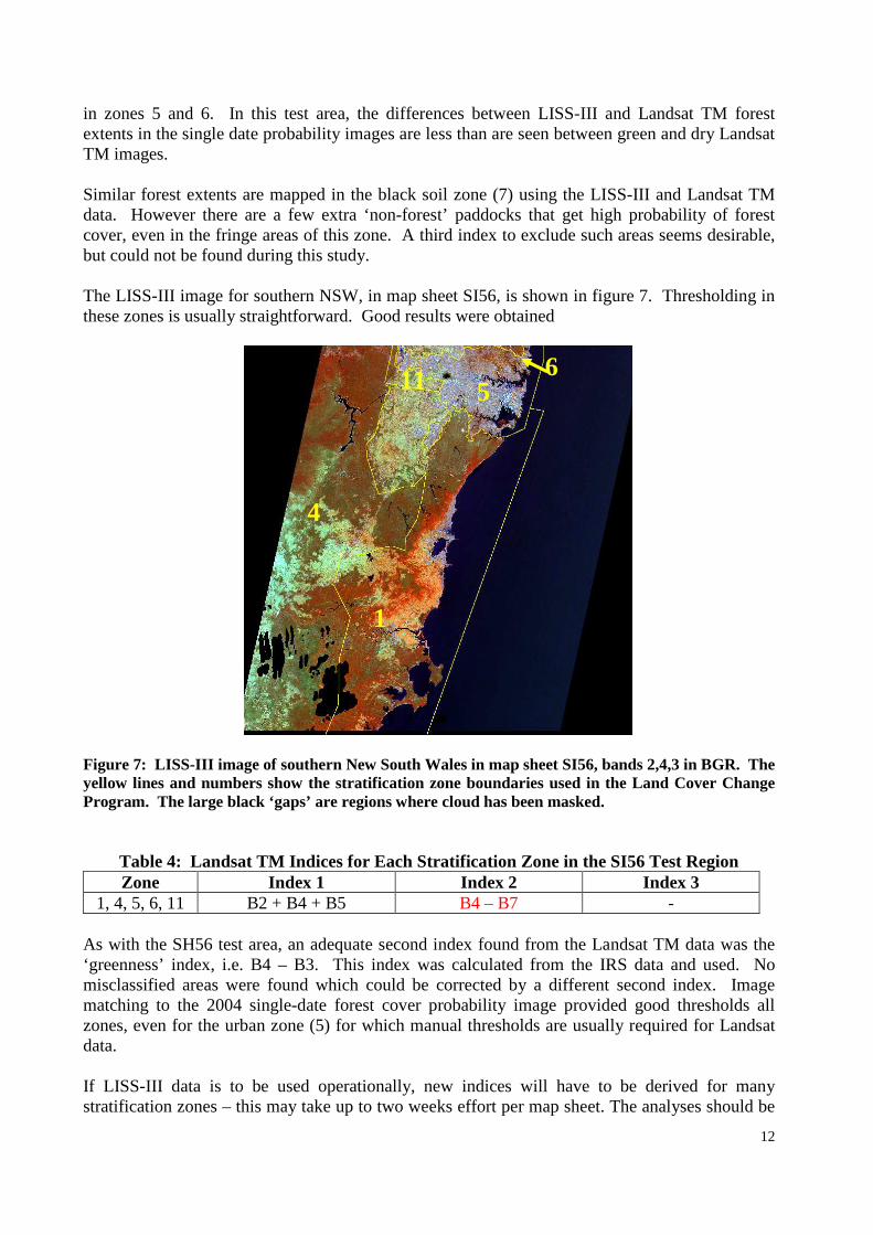
in zones 5 and 6. In this test area, the differences between LISS-III and Landsat TM forest extents in the single date probability images are less than are seen between green and dry Landsat TM images. Similar forest extents are mapped in the black soil zone (7) using the LISS-III and Landsat TM data. However there are a few extra ‘non-forest’ paddocks that get high probability of forest cover, even in the fringe areas of this zone. A third index to exclude such areas seems desirable, but could not be found during this study. The LISS-III image for southern NSW, in map sheet SI56, is shown in figure 7. Thresholding in these zones is usually straightforward. Good results were obtained Figure 7: LISS-III image of southern New South Wales in map sheet SI56, bands 2,4,3 in BGR. The yellow lines and numbers show the stratification zone boundaries used in the Land Cover Change Program. The large black ‘gaps’ are regions where cloud has been masked.

Table 4: Landsat TM Indices for Each Stratification Zone in the SI56 Test Region Zone Index 1 Index 2 Index 3

1, 4, 5, 6, 11 B2 + B4 + B5 B4 – B7 - As with the SH56 test area, an adequate second index found from the Landsat TM data was the ‘greenness’ index, i.e. B4 – B3. This index was calculated from the IRS data and used. No misclassified areas were found which could be corrected by a different second index. Image matching to the 2004 single-date forest cover probability image provided good thresholds all zones, even for the urban zone (5) for which manual thresholds are usually required for Landsat data. If LISS-III data is to be used operationally, new indices will have to be derived for many stratification zones – this may take up to two weeks effort per map sheet. The analyses should be

5

1

4

11 6

13

performed by a very experienced team. Ideally indices are derived by considering two or more image dates to ensure they are robust through time rather than tailored to particular conditions in a single image. All indices derived for the first epoch using IRS LISS-III data should be reviewed when a second epoch is available. Once indices have been established, the overall thresholding effort is slightly increased compared to Landsat TM data. Stratification zones are intersected with the image date boundaries to determine sub-zones. Thresholds are derived for each sub-zone separately. As there are approximately twenty five percent more LISS-III images for complete coverage, there will be approximately twenty five percent more sub-zones to consider and potentially (in the worst case) up to twenty five percent more effort required. 8.2 AWiFS data Thresholding was performed for three stratifications in the SH56 map sheet using the 50m AWiFs imagery. The aims were to

• compare the performance of the AWiFS and LISS-III data where the test images overlap (zones 5 and 6); and

• assess the discrimination of forest and non-forest cover in the centre of the black soil zone (zone 7).

The intention was that by combining these results, it might be possible to infer how well forest and non-forest cover can be discriminated in the centre of the black soil zone. Unfortunately, the AWiFs and LISS-III images were acquired twelves months apart in quite different seasons. Most of the 2004 AWiFs image is much greener than the 2005 LISS-III image. The test region is shown in figure 8. Figure 8: AWiFS image of northern New South Wales in map sheet SH56, bands 2,4,3 in BGR. The yellow lines and numbers show the stratification zone boundaries used in the Land Cover Change Program. The large black ‘gaps’ are regions where cloud has been masked.

7

5

6

14

For zones 5 and 6 the same indices were used as for the LISS-III imagery. As expected from 50m data, narrow features do not get high probabilities of forest cover, as shown in figure 9. Otherwise the forest / non-forest discrimination in local areas appears comparable to that from the LISS-III data. Normally image date boundaries are intersected with the stratification zone boundaries to define sub-zones. Separate thresholds are estimated for each sub-zone to allow for slight seasonal differences between the images. AWiFS scenes are much larger than the stratification zones, so few if any sub-zones will result. However, for larger stratification zones seasonal differences are observed in the imagery across the zone. Applying different thresholds to subregions within the zone would provide better results and some alternative form of creating sub-zones, most likely manual, is required. Figure 9: Top Left: 2004 AWiFS image (bands 2, 4, 3 in BGR). Bottom Left: 2004 Landsat 5 TM imagery (bands 3,5,4 in BGR). Top right: Overlay of the 2004 forest cover probability images derived from the Landsat 5 (red) and AWiFS (green) images. Bottom right: Overlay of the forest cover probability images derived from 2004 Landsat 5 (red) and 2005 LISS-III (green) images.

15

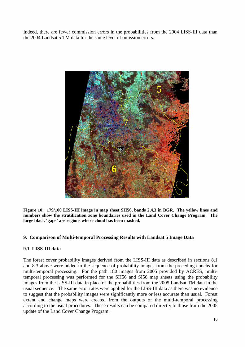
When the indices derived from the LISS-III image for zone 7 were applied to the AWiFS data extensive omission and commission errors were observed. The errors occurred both in the overlapping ‘fringe’ areas of the zone as well as in the centre of the zone. It is likely that the optimal indices derived for the seasonal conditions in the small region of the LISS-III imagery are not robust enough spatially or temporally. New indices were derived from the AWiFS data. Using Landsat TM equivalent band numbers the new indices are 2B2 + 2B3 –B4, 4B2 + B4 – B5 and B4-B3. Over strictly black soils regions the results are broadly similar to those expected from Landsat TM data. However, to prevent omission errors on dense forest, slightly more commission errors were made than is usual for optimal Landsat TM images. Unlike with Landsat TM data, the errors were not whole paddocks getting very high probability of forest cover, but smaller areas adjacent to wooded areas getting moderate probabilities. If not repeated in the same locations in subsequent epochs, the multi-temporal processing is more likely to correct such probabilities. On the fringes of the zone where small patches of black soils mix with larger areas of other soils types, extensive errors (usually omission) were made on the other soil types. The Landsat TM indices were far less sensitive to soil changes in these fringe areas, so the stratification zone boundaries were created to enclose all black soils and some other soils within the ‘black soils’ zones. To get equivalent accuracies the stratification zone boundaries were redrawn for the AWiFS data to exclude as much of the other soils types as possible, and consequently some of the smaller patches of black soils as well. All of the area processed as the black soil zone in the LISS-III data is outside the redrawn zone boundary from the AWiFS data. Thus there is no direct comparison of the forest cover mapping from the two data types. With redrawn stratification zones, it may be possible to produce results similar to those from Landsat TM data using LISS-III data, but obtaining a test image over the centre of the stratification zone is recommended to fully evaluate the discrimination using 7-bit data instead of the 10-bit AWiFS data. 8.3 Satellite Data Australia LISS-III data (path 179) As the sample data provided by ACRES did not allow evaluation of the discrimination of forest and non-forest cover over a typical black soil zone, as described above, additional imagery over such regions was sought. Satellite Data Australia Pty Ltd provided an image from path 179 row 100 acquired on 1 March 2004, approximately two weeks after the AWiFS image provided by ACRES. The image is immediately to the west (and 12 months prior) to the LISS-III image from map sheet SH56 provided by ACRES. It covers most of the NSW black soil zone, as shown in Figure 10. Only the black soil zone was processed. As indicated in table 3, the indices used for the black soil zone (7) use spectral bands not found in the LISS-III data. Training sites of forest and non-forest cover were selected from image inspection using the Landsat TM 2004 forest extent map as ground-truth and new indices derived. The indices, expressed in TM equivalent band numbers, are 2B2 +2B3 - B5, B2 + B3 +B5 and B4 – B3. Similar, but not quite as good, results were obtained when the indices derived for this zone using the SPOT 4 data were applied (B2 + B3 + B5, B2 + B4 and 6B2 – B4 – 2B5 in Landsat TM equivalent band numbers). Image matching to the 2005 (Landsat TM) single-date forest cover probability image provided good thresholds. The results are very consistent with those expected from Landsat TM imagery.

16

Indeed, there are fewer commission errors in the probabilities from the 2004 LISS-III data than the 2004 Landsat 5 TM data for the same level of omission errors. Figure 10: 179/100 LISS-III image in map sheet SH56, bands 2,4,3 in BGR. The yellow lines and numbers show the stratification zone boundaries used in the Land Cover Change Program. The large black ‘gaps’ are regions where cloud has been masked. 9. Comparison of Multi-temporal Processing Results with Landsat 5 Image Data 9.1 LISS-III data The forest cover probability images derived from the LISS-III data as described in sections 8.1 and 8.3 above were added to the sequence of probability images from the preceding epochs for multi-temporal processing. For the path 180 images from 2005 provided by ACRES, multi-temporal processing was performed for the SH56 and SI56 map sheets using the probability images from the LISS-III data in place of the probabilities from the 2005 Landsat TM data in the usual sequence. The same error rates were applied for the LISS-III data as there was no evidence to suggest that the probability images were significantly more or less accurate than usual. Forest extent and change maps were created from the outputs of the multi-temporal processing according to the usual procedures. These results can be compared directly to those from the 2005 update of the Land Cover Change Program.

6

7

5

17

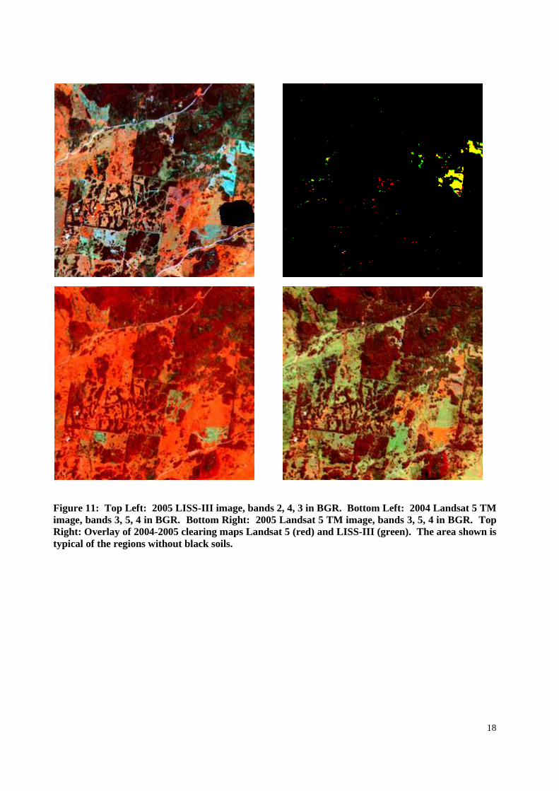
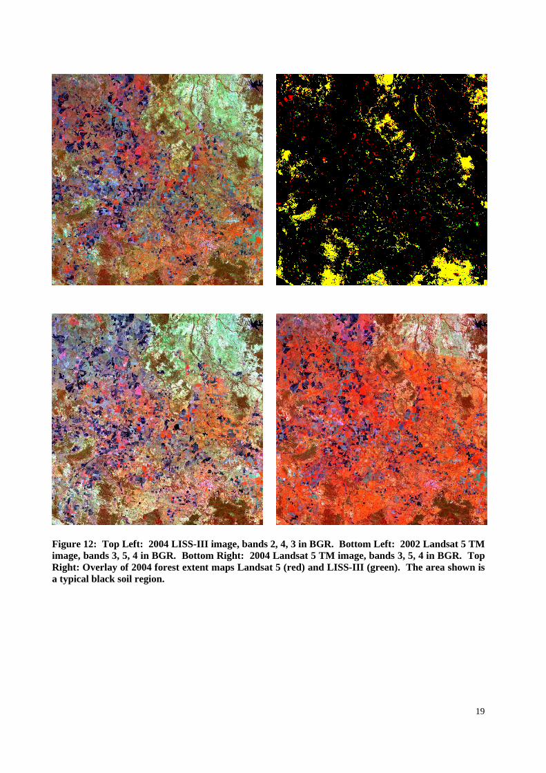
For the path 179 images from 2004, multi-temporal processing was performed for the SH56 map sheet using the probability images from the LISS-III data in place of the probabilities from the 2004 Landsat TM data. To allow common comparison with the results from the path 180 images and with the Landsat 7 SLC-off and SPOT 4 sensors, only data from 1972 to 2004 was processed, i.e. in each case the data from the new sensor is the last component in the sequence with no follow-up data from the Landsat 5 or other sensors. Figure 11 shows the forest cover products for a region in stratification zone 2 in the SH56 test area. The LISS-III image for 2005 is displayed in the top left. The Landsat 5 images for 2004 and 2005 are displayed in the bottom left and bottom right respectively. An overlay of the 2004-2005 clearing maps for the sequences is displayed in the top right. The clearing map from the ‘all Landsat’ sequence is shown in red and the clearing map from the sequence including the LISS-III data is shown in green. Where these products agree, clearing is shown in yellow and no change is shown in black. Regions of red or green are clearing in one product but not the other. There is good agreement between the products from the two sequences in regions of land use change, as shown in the right of figure 11. Both products show a similar level of scattered ‘change’ pixels (both clearing and regrowth) around the edge of forest regions; however the location of such change differs between the two products. The 2004 and 2005 Landsat images that cover the SH56 test area include some very green images and images with a very low sun-angle and hence residual terrain effects. The scatter of change mapped from 2004 to 2005 in the sequence with the 2005 LISS-III image appears little more than the false change mapped as a consequence of the less than optimal Landsat 5 images. Similar results were observed for the SI56 test region. Figure 12 shows similar products for a region in the black soil zone. The LISS-III image for 2004 is displayed in the top left. The Landsat 5 images for 2002 and 2004 are displayed in the bottom left and bottom right respectively. An overlay of the 2004 forest extent maps for the sequences is displayed in the top right. Where these products agree, forest is shown in yellow and non-forest cover is shown in black. Regions of red or green are mapped as forest in one product but not the other. The areas mapped as forest by both sequences (yellow) are all true forest cover and the extents are generally the same. The areas shown in red and green in figure 12 are all commission errors – a common occurrence in black soil zones. Higher levels of such errors are seen in the forest extent maps at the beginning and end of the sequence. Many, but not all, of these are corrected when the next epoch is added to the sequence. The forest extent map from the all-Landsat sequence shows more of these commission errors (red) than from the sequence with the LISS-III image (green). This is not unexpected from the greener 2004 Landsat 5 TM image.

18

Figure 11: Top Left: 2005 LISS-III image, bands 2, 4, 3 in BGR. Bottom Left: 2004 Landsat 5 TM image, bands 3, 5, 4 in BGR. Bottom Right: 2005 Landsat 5 TM image, bands 3, 5, 4 in BGR. Top Right: Overlay of 2004-2005 clearing maps Landsat 5 (red) and LISS-III (green). The area shown is typical of the regions without black soils.

19

Figure 12: Top Left: 2004 LISS-III image, bands 2, 4, 3 in BGR. Bottom Left: 2002 Landsat 5 TM image, bands 3, 5, 4 in BGR. Bottom Right: 2004 Landsat 5 TM image, bands 3, 5, 4 in BGR. Top Right: Overlay of 2004 forest extent maps Landsat 5 (red) and LISS-III (green). The area shown is a typical black soil region.

20

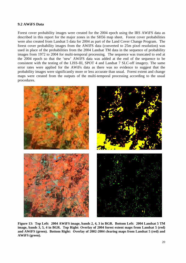
9.2 AWiFS Data Forest cover probability images were created for the 2004 epoch using the IRS AWiFS data as described in this report for the major zones in the SH56 map sheet. Forest cover probabilities were also created from Landsat 5 data for 2004 as part of the Land Cover Change Program. The forest cover probability images from the AWiFS data (converted to 25m pixel resolution) was used in place of the probabilities from the 2004 Landsat TM data in the sequence of probability images from 1972 to 2004 for multi-temporal processing. The sequence was truncated to end at the 2004 epoch so that the ‘new’ AWiFS data was added at the end of the sequence to be consistent with the testing of the LISS-III, SPOT 4 and Landsat 7 SLC-off imagery. The same error rates were applied for the AWiFs data as there was no evidence to suggest that the probability images were significantly more or less accurate than usual. Forest extent and change maps were created from the outputs of the multi-temporal processing according to the usual procedures.

Figure 13: Top Left: 2004 AWiFS image, bands 2, 4, 3 in BGR. Bottom Left: 2004 Landsat 5 TM image, bands 3, 5, 4 in BGR. Top Right: Overlay of 2004 forest extent maps from Landsat 5 (red) and AWiFS (green). Bottom Right: Overlay of 2002-2004 clearing maps from Landsat 5 (red) and AWiFS (green).

21

Figure 13 shows the forest cover products for a region in stratification zone 6 in the SH56 test area. The AWiFS image for 2004 is displayed in the top left. The Landsat 5 image for 2004 is displayed in the bottom left. Overlays of the 2004 forest extent and the 2002-2004 clearing maps for the sequences are displayed in the top right and bottom right respectively. The products from the ‘all Landsat’ sequence are shown in red and the products from the sequence including the AWiFS data are shown in green. Where these products agree, forest/clearing is shown in yellow and non-forest/no change is shown in black. Regions of red or green are forest/clearing in one product but not the other. As expected, the coarser resolution of the AWiFS data means that narrow features such as streamline and roadside trees are not mapped as forest in 2004 by the sequence including the AWiFs data (appear in red only in the forest extent map in the top right of figure 13 and as green only in the clearing map). Differences in the pixels mapped as forest around the edge of larger forest blocks are also observed. This is similar to the differences observed between products from the Landsat MSS and TM epochs around 1989 in the current sequence. This effect is observed across all stratification zones, including the black soils zone. 10. Conclusions Individual ‘map’ oriented LISS-III and AWiFS images can be adequately registered to the AGO base images with minimal additional ‘per image’ effort. There is no reason to expect different results for ‘path’ oriented imagery. Additional Master GCP features may be required for some images as the existing features used with Landsat images may not provide a sufficiently dense spatial coverage for the smaller LISS-III scenes. The ortho-rectification effort will be increase by a small ‘per image’ amount corresponding to increasing the number of Master GCPs, as well as by the increased number of images to be processed. If AWiFs imagery were to be used operationally, some consideration would need to be given to the consequences of the 740km image width. Landsat TM images are ortho-rectified to the MGA zone that includes the majority of the image. Parts of each image (up to half the 200km image width) may be reprojected into the adjacent zone, if necessary, during mosaicing. The difference between reprojecting data up to 370km beyond the zone edge and splitting the image to ortho-rectify directly to each zone (or ortho-rectifying the whole image twice) needs to be investigated, including the potential consequences increased file handling. Calibration of the IRS imagery requires extensive further study. New BRDF kernels may need to be derived as well as new model coefficients. Much more data is required to establish appropriate models (the Landsat models and coefficients were derived from about thirty scenes covering the whole of Queensland). As the intensity range of the LISS-III and AWiFS imagery is much greater than for the Landsat TM imagery, a new calibration base will need to be investigated, particularly if the data is to be later used to monitor trends. As with the Master GCPs, the invariant target locations used in the calibration process may be too sparsely located for the smaller images. Once appropriate methodologies have been established, the operational processing effort should only increase by the ‘per image’ amount necessary for the selection of new invariant targets.

22

In the thresholding stage of the processing, new indices will have to be derived for most stratification zones as not all Landsat TM spectral bands are present in the IRS image data. This may take up to two weeks of effort per map sheet. The analyses should be performed by a very experienced team. Ideally indices are derived by considering two or more image dates to ensure they are robust through time rather than tailored to particular conditions in a single image. All indices derived for the first epoch using IRS data should be reviewed when a second epoch is available. Once indices have been established, the overall thresholding effort is increased compared to Landsat TM data, in the worst case by the number of extra scenes required for complete coverage. Normally image date boundaries are intersected with the stratification zone boundaries to define sub-zones. Separate thresholds are estimated for each sub-zone to allow for slight seasonal differences between the images. AWiFS scenes are much larger than the stratification zones, so few, if any, sub-zones will results. However, for larger stratification zones seasonal differences are observed in the imagery across the zone. Applying different thresholds to subregions within the zone would provide better results and some alternative form of creating sub-zones, most likely manual, is required. The forest cover extent and change products from the LISS-III are more consistent with those obtained from Landsat 5 or Landsat 7 SLC-off data than those from the SPOT 4 data tested over the stratification zones not containing black soils (Furby et al, 2006a and 2006b). All products correctly identify genuine land cover change in such zones. The rates of change between the LISS-III epoch and the rest of the sequence appear similar to those from the Landsat 5 and Landsat 7 SLC-off sequences, although generally the particular pixels of scattered change and the cover types for which commission errors are made in the black soil zones differ. The forest extent and change products from the AWiFS data show significant additional areas of change on small or narrow features and the edges of larger forest regions, an expected consequence of the coarser spatial resolution. These are similar to the effects between the Landsat MSS and TM epochs around 1989 in the current Landsat sequence. For this reason, LISS-III imagery would be the preferred option. 11. References Furby, S. L. (2006), Documentation for the 2005 Update of the Forest Cover Mapping for the Australian Greenhouse Office Land Use Change Program, CSIRO Mathematical and Information Sciences Technical Report 06/43. Furby, S. L. and Wu, X. (2006a), Evaluation of Landsat 7 SLC-off Image Data for Forest Cover Mapping, CSIRO Mathematical and Information Sciences Technical Report 06/154. Furby, S. L., Wu, X. and O’Connell, J. (2006b), Evaluation of SPOT 4 Image Data for Forest Cover Mapping, CSIRO Mathematical and Information Sciences Technical Report 06/155. Resourcesat -1 (IRS-P6) Data User’s Handbook, National remote Sensing Agency, Department of Space, Government of India.