Technical Report Documentation Page 1. Report No. FHWA/TX-14/0-6804-1 2. Government Accession No. 3. Recipient’s Catalog No. 4. Title and Subtitle Evaluation of Lightweight Noise Barrier on IH-30 Bridge Structure in Dallas, Texas 5. Report Date August 2014; Published March 2015 6. Performing Organization Code 7. Author(s) Manuel Trevino 8. Performing Organization Report No. 0-6804-1 9. Performing Organization Name and Address Center for Transportation Research The University of Texas at Austin 1616 Guadalupe Street, Suite 4.202 Austin, TX 78701 10. Work Unit No. (TRAIS) 11. Contract or Grant No. 0-6804 12. Sponsoring Agency Name and Address Texas Department of Transportation Research and Technology Implementation Office P.O. Box 5080 Austin, TX 78763-5080 13. Type of Report and Period Covered Technical Report. January 2013–July 2014 14. Sponsoring Agency Code 15. Supplementary Notes Project performed in cooperation with the Texas Department of Transportation and the Federal Highway Administration. 16. Abstract The Texas Department of Transportation commissioned a study to analyze the feasibility and effectiveness of a lightweight noise barrier on Interstate Highway 30, near downtown Dallas. The highway segment in question, an elevated structure next to a creek, has presented noise problems for the adjacent neighborhood ever since its expansion in the early 2000s. The highway carries substantial commuter traffic as well as heavy trucks. The neighborhood is hilly and sits at a higher elevation relative to the highway, except for a few residences on the street adjacent to the creek. The material for the noise barrier needed to be lightweight in order to be supported by the existing bridge structures without having to retrofit them. A 10-ft tall transparent acrylic noise barrier was designed to be installed on top of the existing 8-ft concrete wall. Residential sound pressure level tests were performed at various locations for five months before the transparent wall installation, and continued for nine months after the wall was completed. A portable weather station was used to monitor the conditions at the time of the tests. Measurements were conducted three times a day—morning, afternoon, and evening—and test days occurred once or twice a month. A statistical analysis of the various weather variables and their influence on the noise levels was performed. The results indicate that the wall is effective for certain receivers; although the acoustic benefits appear to be small, they are statistically significant, showing that the barrier has an effect on noise levels. The neighbors are satisfied with its performance and with its aesthetic appearance. 17. Key Words Traffic noise, noise barrier, lightweight material, transparent material, aesthetics, visual impact, noise mitigation 18. Distribution Statement No restrictions. This document is available to the public through the National Technical Information Service, Springfield, Virginia 22161; www.ntis.gov. 19. Security Classif. (of report) Unclassified 20. Security Classif. (of this page) Unclassified 21. No. of pages 118 22. Price Form DOT F 1700.7 (8-72) Reproduction of completed page authorized
Transcript
Technical Report Documentation Page
1. Report No.
FHWA/TX-14/0-6804-1
2. Government Accession No.
3. Recipient’s Catalog No.
4. Title and Subtitle
Evaluation of Lightweight Noise Barrier on IH-30 Bridge Structure in Dallas, Texas
5. Report Date
August 2014; Published March 2015
6. Performing Organization Code 7. Author(s)
Manuel Trevino
8. Performing Organization Report No.
0-6804-1
9. Performing Organization Name and Address
Center for Transportation Research The University of Texas at Austin 1616 Guadalupe Street, Suite 4.202 Austin, TX 78701
10. Work Unit No. (TRAIS) 11. Contract or Grant No.
0-6804
12. Sponsoring Agency Name and Address
Texas Department of Transportation Research and Technology Implementation Office P.O. Box 5080 Austin, TX 78763-5080
13. Type of Report and Period Covered
Technical Report. January 2013–July 2014
14. Sponsoring Agency Code
15. Supplementary Notes Project performed in cooperation with the Texas Department of Transportation and the Federal Highway Administration.
16. Abstract
The Texas Department of Transportation commissioned a study to analyze the feasibility and effectiveness of a lightweight noise barrier on Interstate Highway 30, near downtown Dallas. The highway segment in question, an elevated structure next to a creek, has presented noise problems for the adjacent neighborhood ever since its expansion in the early 2000s. The highway carries substantial commuter traffic as well as heavy trucks. The neighborhood is hilly and sits at a higher elevation relative to the highway, except for a few residences on the street adjacent to the creek. The material for the noise barrier needed to be lightweight in order to be supported by the existing bridge structures without having to retrofit them. A 10-ft tall transparent acrylic noise barrier was designed to be installed on top of the existing 8-ft concrete wall. Residential sound pressure level tests were performed at various locations for five months before the transparent wall installation, and continued for nine months after the wall was completed. A portable weather station was used to monitor the conditions at the time of the tests. Measurements were conducted three times a day—morning, afternoon, and evening—and test days occurred once or twice a month. A statistical analysis of the various weather variables and their influence on the noise levels was performed. The results indicate that the wall is effective for certain receivers; although the acoustic benefits appear to be small, they are statistically significant, showing that the barrier has an effect on noise levels. The neighbors are satisfied with its performance and with its aesthetic appearance.
No restrictions. This document is available to the public through the National Technical Information Service, Springfield, Virginia 22161; www.ntis.gov.
19. Security Classif. (of report) Unclassified
20. Security Classif. (of this page) Unclassified
21. No. of pages 118
22. Price
Form DOT F 1700.7 (8-72) Reproduction of completed page authorized
Evaluation of Lightweight Noise Barrier on IH-30 Bridge Structure in Dallas, Texas Manuel Trevino CTR Technical Report: 0-6804-1 Report Date: August 2014; Published March 2015 Project: 0-6804 Project Title: Life Cycle Cost and Performance of Lightweight Noise Barrier Materials
Along Bridge Structures Sponsoring Agency: Texas Department of Transportation Performing Agency: Center for Transportation Research at The University of Texas at Austin Project performed in cooperation with the Texas Department of Transportation and the Federal Highway Administration.
Center for Transportation Research The University of Texas at Austin 1616 Guadalupe, Suite 4.202 Austin, TX 78701 http://ctr.utexas.edu/
v
Disclaimers Author's Disclaimer: The contents of this report reflect the views of the authors, who
are responsible for the facts and the accuracy of the data presented herein. The contents do not necessarily reflect the official view or policies of the Federal Highway Administration or the Texas Department of Transportation (TxDOT). This report does not constitute a standard, specification, or regulation.
Patent Disclaimer: There was no invention or discovery conceived or first actually reduced to practice in the course of or under this contract, including any art, method, process, machine manufacture, design or composition of matter, or any new useful improvement thereof, or any variety of plant, which is or may be patentable under the patent laws of the United States of America or any foreign country.
Engineering Disclaimer NOT INTENDED FOR CONSTRUCTION, BIDDING, OR PERMIT PURPOSES.
vi
Acknowledgments The author expresses gratitude to Mr. Bill Hale and Mr. George Reeves, with TxDOT,
Dallas District, for their support and advice. The guidance of Mr. Rob Harrison, and Mr. Duncan Stewart, with CTR, and Mr. Wade Odell, with TxDOT, as well as the assistance of Mr. Mark McIlheran, with Armtec/Acrylite, are also appreciated. Many thanks to those who were consulted for their expertise in transparent noise barriers for sharing their knowledge and experiences.
The cooperation of the Kessler Park neighbors is acknowledged, especially those who kindly allowed the researcher to perform the measurements in their property at all times of the day.
1.2.1 Objective and Tasks ........................................................................................................2 1.3 Report Organization ...............................................................................................................2
Chapter 2. Review of Experiences and Literature ......................................................................5 2.1 Introduction ............................................................................................................................5 2.2 Noise Barriers and Material Selection ...................................................................................6
2.2.2 Aesthetics and Transparent Barriers ...............................................................................7 2.3 The Experiences of Various Organizations ...........................................................................8
2.3.1 Ohio DOT .......................................................................................................................8 2.3.2 The FHWA ......................................................................................................................8 2.3.3 Acrylite ...........................................................................................................................8 2.3.4 Plaskolite .........................................................................................................................9 2.3.5 AIL Sound Walls ............................................................................................................9
Chapter 5. Noise Testing Program .............................................................................................33 5.1 Introduction ..........................................................................................................................33 5.2 Test Equipment and Procedure ............................................................................................33 5.3 Test Locations ......................................................................................................................40
5.3.1 Site 1 Locations .............................................................................................................40 Location E ......................................................................................................................... 42 Location D ........................................................................................................................ 43 Location F ......................................................................................................................... 45 Location C ......................................................................................................................... 46 Location B ......................................................................................................................... 47
Chapter 6. Test Results and Analysis .........................................................................................59 6.1 Analysis of Overall Results and TNM Predictions ..............................................................59
6.1.1 Site 1 .............................................................................................................................59 6.1.2 Site 2 .............................................................................................................................61
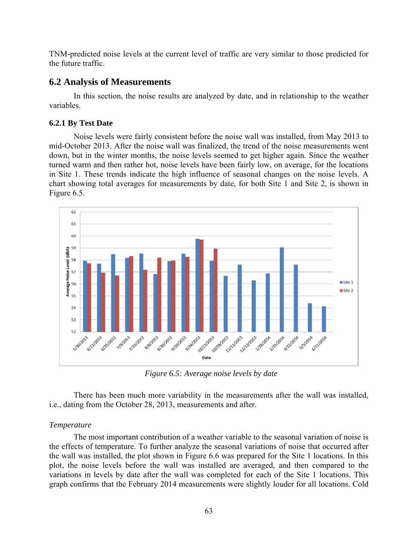
6.2 Analysis of Measurements ...................................................................................................63 6.2.1 By Test Date .................................................................................................................63
Figure 2.1: Acoustic energy and noise barrier (Bowlby 2012) ....................................................... 6 Figure 2.2: Acrylite Soundstop product samples ............................................................................ 9 Figure 2.3: AIL Sound Walls product sample delivered to CTR showing the absorptive
material (acoustical mineral wool) encased in the PVC stackable panel .......................... 10 Figure 2.4: AIL Sound Walls product sample delivered to CTR: Silent Protector product ......... 10 Figure 2.5: AIL Sound Walls product samples delivered to CTR: Tuf-Barrier product
(reflective) made of PVC .................................................................................................. 11 Figure 3.1: Project location on IH 30............................................................................................ 13 Figure 3.2: Proposed noise barriers for Site 1 and Site 2, on IH 30 ............................................. 14 Figure 3.3: View of IH 30 towards the east from Edgefield Avenue Bridge, showing the
south-side concrete wall on the right ................................................................................ 15 Figure 3.4: IH-30 elevated highway structure and concrete wall, seen from Coombs
Creek (Site 1) .................................................................................................................... 15 Figure 3.5: IH 30 underside of elevated highway structure, seen from below Sylvan
Avenue .............................................................................................................................. 16 Figure 3.6: Coombs Creek, seen from the Sylvan Avenue underpass (Site 1) ............................. 16 Figure 3.7: Coombs Creek, east of Sylvan Ave (Site 2); elevated highway structure in the
background ........................................................................................................................ 17 Figure 3.8: South side wall on IH 30 at Site 1 .............................................................................. 18 Figure 3.9: South side wall on IH 30 at Site 2 .............................................................................. 18 Figure 3.10: Coombs Creek Trail Park, at Site 1 .......................................................................... 19 Figure 3.11: Coombs Creek Trail Park, at Site 2 .......................................................................... 19 Figure 3.12: First row residence on Kessler Parkway, at Site 1 ................................................... 20 Figure 3.13: View from a residence at higher elevation and clear line of sight to IH 30 ............. 20 Figure 3.14: Example of a scenic view from a residence at Site 2 ............................................... 21 Figure 4.1: Receivers for TNM analysis ....................................................................................... 24 Figure 4.2: Plan view of IH-30 TNM model ................................................................................ 25 Figure 4.3: View of IH 30 from Receiver 8 .................................................................................. 29 Figure 4.4: Measurements taken at Site C, on Kessler Parkway .................................................. 30 Figure 4.5: Measurement taken at Site B, the Coombs Creek Trail Park ..................................... 30 Figure 5.1: Sound pressure level meter ......................................................................................... 34 Figure 5.2: Leq(A): average noise level over a period of time ..................................................... 34 Figure 5.3: Davis Instruments portable weather station, showing the ISS ................................... 35 Figure 5.4: Vantage Vue wireless console .................................................................................... 36 Figure 5.5: Weather station mounted in the back of research vehicle .......................................... 36 Figure 5.6: Mirror compass utilized for orientation of the weather station .................................. 37
x
Figure 5.7: Use of the mirror compass for orientation of the weather station: the solar panel of the weather station, in the background, is positioned so that it faces south ....... 38
Figure 5.8: Weather plots of daily records generated by WeatherLink ........................................ 39 Figure 5.9: WeatherLink screen showing weather records for every minute ............................... 40 Figure 5.10: Site 1 noise measurement locations.......................................................................... 41 Figure 5.11: Residential measurement at Location E ................................................................... 42 Figure 5.12: Residential measurement at Location E ................................................................... 43 Figure 5.13: Residential measurement at Location D ................................................................... 44 Figure 5.14: Residential measurement at Location D ................................................................... 44 Figure 5.15: Residential measurement at Location F ................................................................... 45 Figure 5.16: Residential measurement at Location F ................................................................... 46 Figure 5.17: Residential measurement at Location C ................................................................... 46 Figure 5.18: Residential measurement at Location C ................................................................... 47 Figure 5.19: Noise measurement at Coombs Creek Trail Park (Location B) prior to noise
barrier installation ............................................................................................................. 48 Figure 5.20: Noise measurement at Coombs Creek Trail Park (Location B) after noise
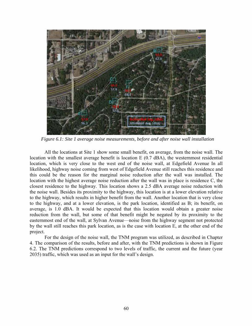
barrier installation ............................................................................................................. 48 Figure 5.21: Site 2 noise measurement locations.......................................................................... 49 Figure 5.22: Residential measurement at Location R3 ................................................................. 50 Figure 5.23: Residential measurement at Location R3, with TxDOT’s George Reeves .............. 51 Figure 5.24: Residential measurement at Location R8 ................................................................. 52 Figure 5.25: IH-30 view from residence at Location R8 .............................................................. 52 Figure 5.26: Residential measurement at Location R12 ............................................................... 53 Figure 5.27: Residential measurement at Location R12 ............................................................... 54 Figure 5.28: Residential measurement at Location R13 ............................................................... 55 Figure 5.29: Residential measurement at Location R13 ............................................................... 55 Figure 5.30: Noise measurement at Coombs Creek Trail Park (Location R27) ........................... 56 Figure 5.31: Noise measurement at Coombs Trail Park (Location R27) ..................................... 57 Figure 6.1: Site 1 average noise measurements, before and after noise wall installation ............. 60 Figure 6.2: Site 1 average noise measurements, before and after noise wall installation,
compared with TNM predictions ...................................................................................... 61 Figure 6.3: Site 2 average noise measurements, before noise wall installation ............................ 62 Figure 6.4: Site 2 average noise measurements, before noise wall installation, compared
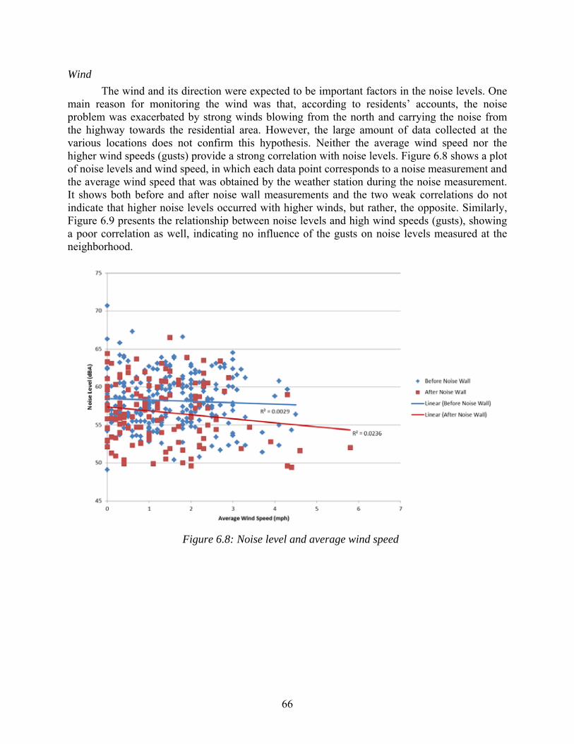
with TNM predictions ....................................................................................................... 62 Figure 6.5: Average noise levels by date ...................................................................................... 63 Figure 6.6: Noise levels before and after wall, for Site 1 locations .............................................. 64 Figure 6.7: Noise level and temperature ....................................................................................... 65 Figure 6.8: Noise level and average wind speed ........................................................................... 66 Figure 6.9: Noise level and high wind speed ................................................................................ 67
xi
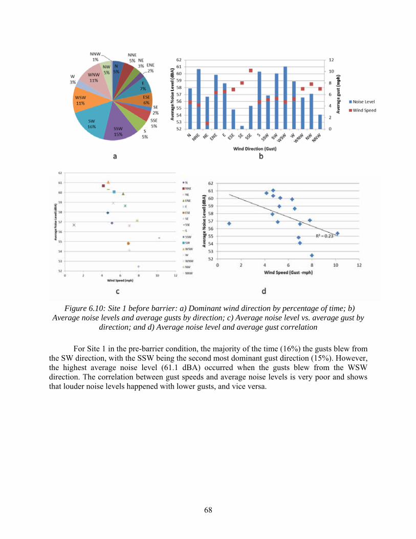
Figure 6.10: Site 1 before barrier: a) Dominant wind direction by percentage of time; b) Average noise levels and average gusts by direction; c) Average noise level vs. average gust by direction; and d) Average noise level and average gust correlation ....... 68
Figure 6.11: Site 1 after barrier: a) Dominant wind direction by percentage of time; b) Average noise levels and average gusts by direction; c) Average noise level vs. average gust by direction; and d) Average noise level and average gust correlation ....... 69
Figure 6.12: Site 2: a) Dominant wind direction by percentage of time; b) Average noise levels and average gusts by direction; c) Average noise level vs. average gust by direction; and d) Average noise level and average gust correlation ................................. 70
Figure 6.13: Noise level and relative humidity ............................................................................. 71 Figure 6.14: Frequency distribution for pre-barrier (a) and post-barrier (b) tests ........................ 72 Figure 6.15: Average frequency spectra for Site 1 locations for pre-barrier and post-
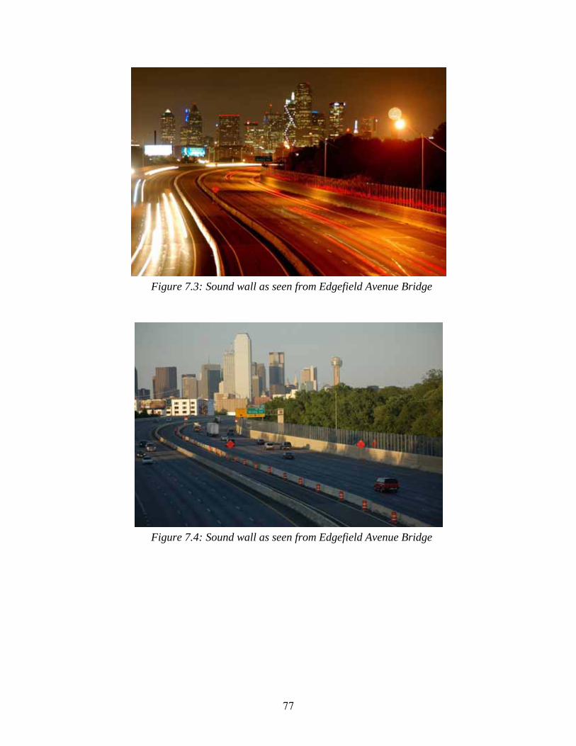
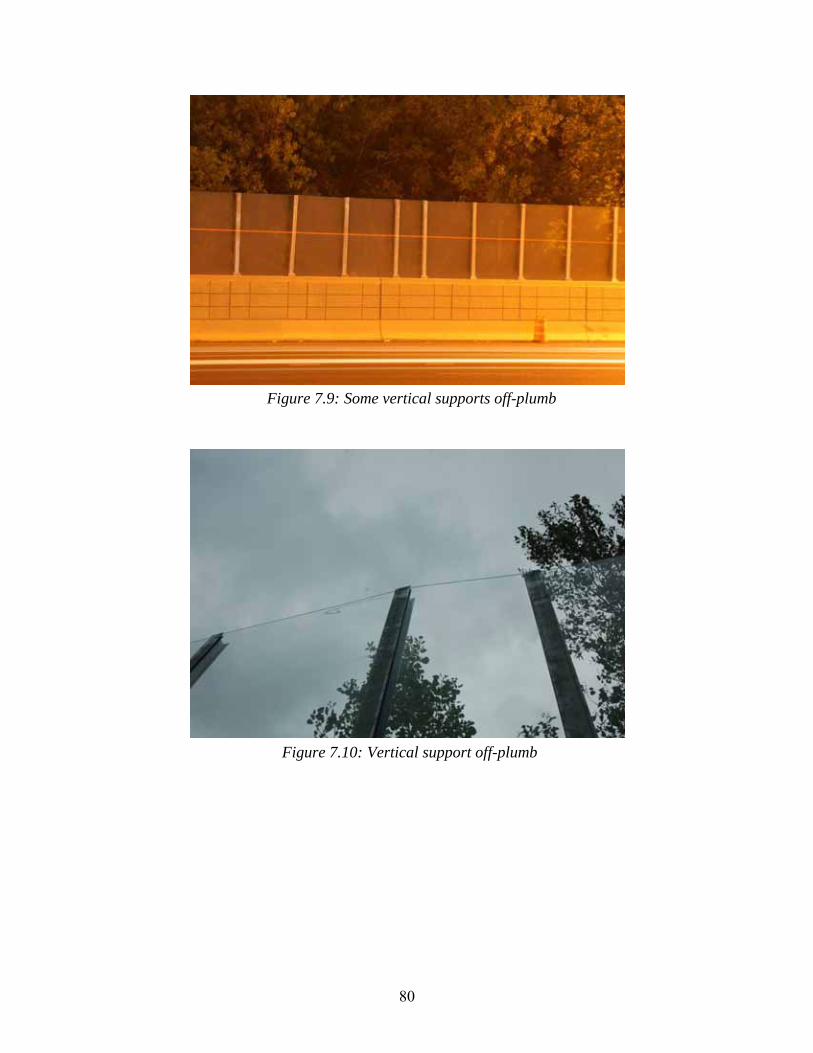
barrier tests ........................................................................................................................ 73 Figure 7.1: Nighttime installation ................................................................................................. 76 Figure 7.2: Vertical support placement ......................................................................................... 76 Figure 7.3: Sound wall as seen from Edgefield Avenue Bridge ................................................... 77 Figure 7.4: Sound wall as seen from Edgefield Avenue Bridge ................................................... 77 Figure 7.5: Sound wall as seen from Edgefield Avenue Bridge ................................................... 78 Figure 7.6: Sound wall as seen from westbound IH 30 ................................................................ 78 Figure 7.7: Sound wall as seen from westbound IH 30 looking towards Edgefield Avenue
Bridge ................................................................................................................................ 79 Figure 7.8: Sound wall as seen from westbound lanes looking towards downtown .................... 79 Figure 7.9: Some vertical supports off-plumb .............................................................................. 80 Figure 7.10: Vertical support off-plumb ....................................................................................... 80 Figure 7.11: Gasket shown protruding from metal support .......................................................... 81 Figure 7.12: Gap between vertical gasket and metal support ....................................................... 82 Figure 7.13: Gap between horizontal gasket and metal support ................................................... 82 Figure 7.14: Armtec’s Mark McIlheran inspecting the wall, showing the gap size between
a panel and the gasket ....................................................................................................... 83 Figure 7.15: Gap in existing concrete wall at bridge expansion joint as seen from Coombs
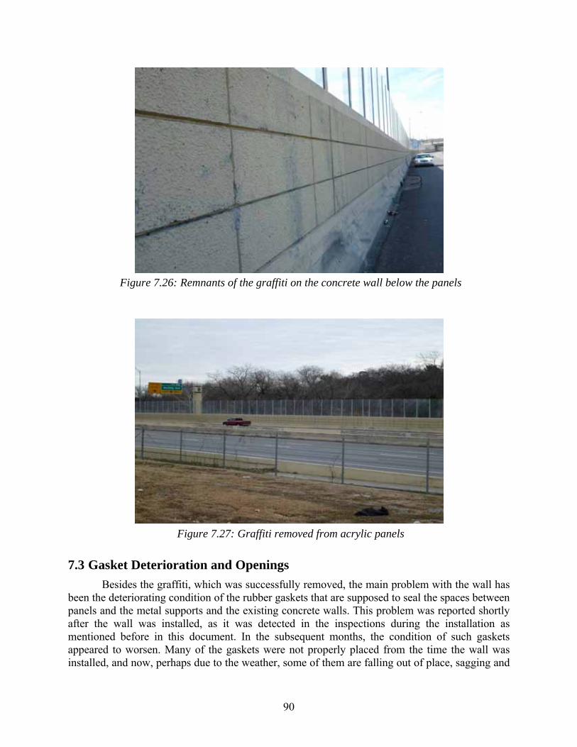
Creek ................................................................................................................................. 84 Figure 7.16: Gap in existing concrete wall at bridge expansion joint as seen from the
highway side ..................................................................................................................... 84 Figure 7.17: Graffiti as seen from the highway shoulder on November 11, 2013 ....................... 85 Figure 7.18: Graffiti as seen from the highway shoulder on November 11, 2013 ....................... 85 Figure 7.19: Graffiti as seen from the highway shoulder on November 11, 2013. The
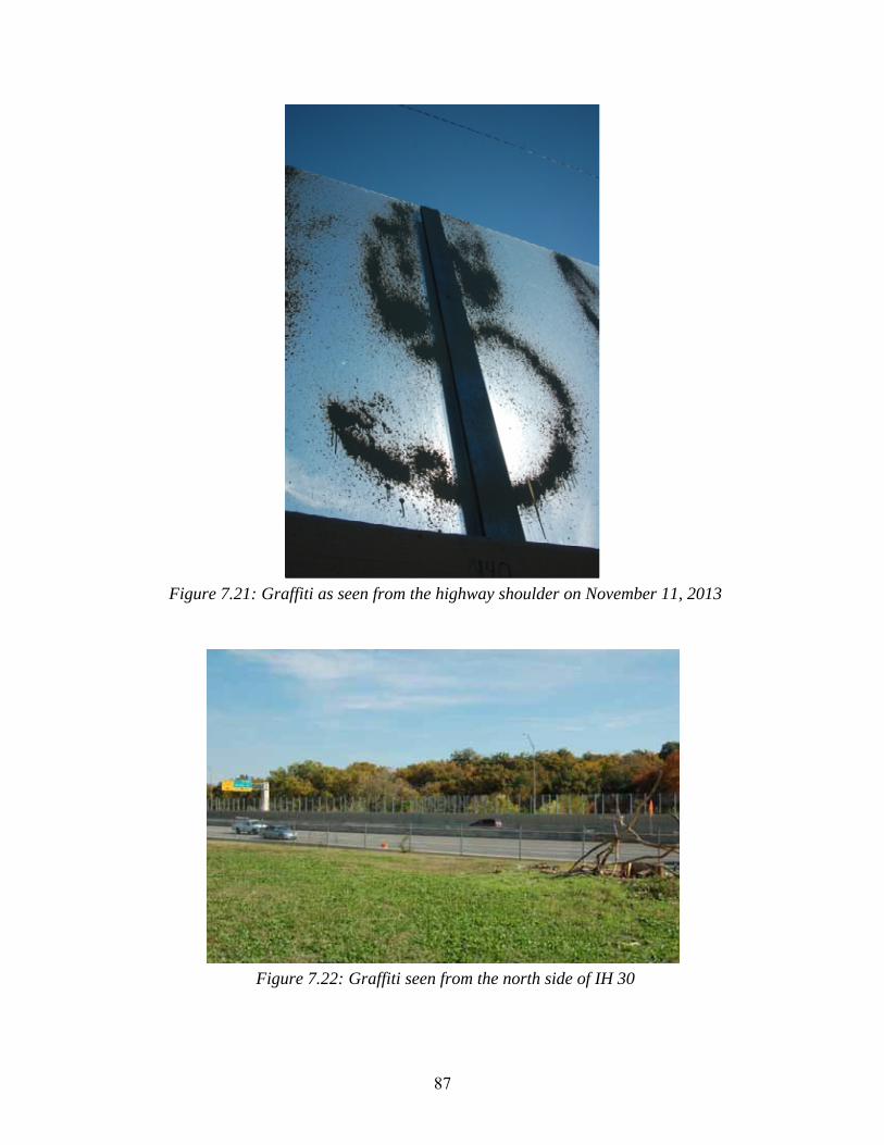
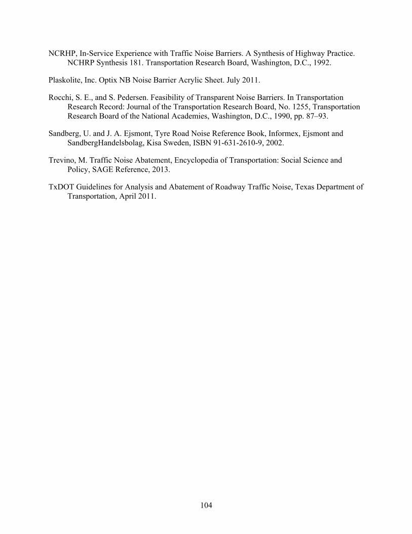
damage extends to the concrete wall under span #144. .................................................... 86 Figure 7.20: Graffiti as seen from the highway shoulder on November 11, 2013 ....................... 86 Figure 7.21: Graffiti as seen from the highway shoulder on November 11, 2013 ....................... 87 Figure 7.22: Graffiti seen from the north side of IH 30 ................................................................ 87
xii
Figure 7.23: Graffiti seen from the north side of IH 30 ................................................................ 88 Figure 7.24: Cleaned panel showing traces of the cleaning operation ......................................... 89 Figure 7.25: Cleaned panel showing traces of the cleaning operation ......................................... 89 Figure 7.26: Remnants of the graffiti on the concrete wall below the panels .............................. 90 Figure 7.27: Graffiti removed from acrylic panels ....................................................................... 90 Figure 7.28: Sagging of horizontal rubber gaskets ....................................................................... 91 Figure 7.29: Sagging of horizontal rubber gaskets ....................................................................... 91 Figure 7.30: Sagging of horizontal rubber gaskets ....................................................................... 92 Figure 7.31: Sagging of horizontal rubber gaskets ....................................................................... 92 Figure 7.32: Broken horizontal rubber gasket .............................................................................. 93 Figure 7.33: Broken horizontal rubber gasket .............................................................................. 93 Figure 7.34: Broken horizontal rubber gasket .............................................................................. 94 Figure 7.35: Vegetation from the creek side growing through the openings in the gaskets
under noise barrier ............................................................................................................ 94 Figure 7.36: Vegetation from the creek side growing through the openings in the gaskets
under noise barrier ............................................................................................................ 95 Figure 7.37: Expansion joint opening due to lack of sealant ........................................................ 96 Figure 7.38: Damaged, old sealant material in the expansion joints of bridge structure .............. 97 Figure 7.39: Vegetation from the creek side growing through the openings in the concrete
structure............................................................................................................................. 98 Figure 8.1: Foliage differences between hot (left) and cold (right) seasons in the
proximity of the barrier ................................................................................................... 100
This is the first report developed under Research Project 0-6804, Life Cycle Cost and Performance of Lightweight Noise Barrier Materials along Bridge Structures, a study funded by the Texas Department of Transportation (TxDOT). This is an interim report produced to document all findings to date about the lightweight noise barrier installed as part of this project, including field data as well as analyses and conclusions derived from the data to date.
1.1 Background
Noise associated with transportation has progressively become a nuisance to communities along roads, especially in densely populated areas. As traffic volumes of people and freight continue to grow, roads expand and noise levels rise. Nowadays, transportation agencies have become more environmentally sensitive and make efforts to address pollution problems, including those related to noise. Multiple factors affect the level of traffic noise, such as vehicle speed, terrain, grade, surface absorption, and shielding provided by walls, fences, buildings, or even dense vegetation. The most frequently used noise abatement measure has been the construction of noise barriers on the side of the road. Such barriers are normally built along highways that carry heavy traffic in urban areas, where noise pollution is likely to be greater and affect more people.
Noise barriers are normally solid wall structures built between the highway and the impacted activity area to reduce noise levels. Barriers do not eliminate the noise; they only reduce the noise levels perceived by certain benefitted receivers, normally those in proximity to the road. Barriers are especially effective for those receivers situated directly behind it; they can experience a decrease in noise level of typically 5 to 10 dBA. Noise barriers are not effective for homes on a hillside overlooking a road, or for buildings that rise above the barrier; the barrier must be high enough and long enough to block the view of the road. Common materials for barrier construction are concrete and masonry; other materials are metal and acrylic.
The height, length, and material are key components to the effectiveness of the barrier. Openings in the barriers, such as those designed to allow access to side roads or driveways, decrease their effectiveness.
Noise barriers can reduce visibility and lighting for both the receivers behind the barrier and the drivers using the facility. Barriers can also present a problem for businesses along the road by restricting views and access by customers. Barriers constructed with transparent materials can address these problems by reducing the visual impact of opaque barriers, and providing aesthetic value by preserving scenic vistas.
1.2 Project Description
The TxDOT Dallas District asked researchers at The University of Texas at Austin’s Center for Transportation Research (UT-CTR) to develop a pilot project to investigate the feasibility of two lightweight noise barriers on Interstate Highway 30 (IH 30), just west of downtown Dallas. The highway segment in question, an elevated structure next to a creek, has presented noise problems for the adjacent neighborhood ever since its expansion in the early 2000s. The highway carries substantial commuter traffic as well as heavy trucks. The material for the noise barriers needed to be lightweight in order to be supported by the existing bridge structures without having to retrofit them. The two adjacent highway sections are the subject of
2
this investigation. The westernmost barrier has already been installed at what has been labeled as Site 1, and the easternmost is part of a future plan, at Site 2. An existing 8-ft tall concrete wall at Site 1 already provided some noise mitigation to the residences. The highway segment under future consideration for a barrier at Site 2 also has an existing 4.5-ft tall concrete barrier. However, the neighborhood is hilly and sits at a higher elevation relative to the highway, except for a few residences on the street adjacent to the creek, so TxDOT wanted to provide a taller barrier to increase the noise abatement, without entirely blocking the views of the residences towards downtown. Therefore, an aesthetic solution was also sought. A 10-ft tall transparent acrylic noise barrier was designed to be installed on top of the existing 8-ft concrete wall at Site 1. Noise barriers are normally not effective for receivers on a hillside overlooking the highway or for receivers at heights above the top of a noise barrier; thus, it was not expected that the residences at the higher elevations would be substantially benefited.
A second noise barrier is proposed for the following stage of this research project, which would be adjacent and similar to the barrier that was designed and installed in the first stage.
The transparent noise barrier that was recommended, designed, and installed as the outcome of the first part of this project was the first one of its kind in Texas. TxDOT’s intent for this project, besides the benefit to Kessler Park (the adjacent neighborhood on the south side of IH 30), is to provide cost and performance information for future project comparisons and, if successful, to develop this type of project on other highways facing similar problems.
1.2.1 Objective and Tasks
The main objective of this study is to assess the feasibility and effectiveness of lightweight noise barriers on IH 30 in Dallas, and to serve as a pilot project for TxDOT for future similar projects. The tasks are as follows:
• Conduct a feasibility study for a lightweight traffic noise wall.
• Select barrier material types and vendors.
• Perform the acoustical design of the barrier.
• Conduct periodic inspections of the barrier condition.
• Perform sound measurements before and after the barrier’s installation.
• Analyze measurements and evaluate performance.
1.3 Report Organization
This report is organized as follows:
• Chapter 1 presents the background and the objectives of the study.
• Chapter 2 reviews vendors’ and various state DOTs’ experiences with and materials used for lightweight and transparent noise barriers.
• Chapter 3 provides a description of the highway and the neighborhood that are the subject of the investigation.
• Chapter 4 discusses the barrier design and recommendation presented to TxDOT’s Dallas District.
3
• Chapter 5 describes the noise testing program.
• Chapter 6 presents the noise test results and analysis.
• Chapter 7 explains the barrier inspection and monitoring, as well as the findings from these activities.
• Chapter 8 discusses the preliminary conclusions of the study up to this stage of the project and the recommendations to TxDOT.
4
5
Chapter 2. Review of Experiences and Literature
2.1 Introduction
This chapter presents a review of various lightweight noise barrier materials considered as candidates for the noise wall installation planned for the south side of the elevated structures on IH 30 in Dallas. Specifically, the project contained the segments between Edgefield Avenue and Sylvan Avenue, as well as from Sylvan Avenue to Beckley Avenue, in the vicinity of the Kessler Park neighborhood.
The need to investigate lightweight materials for the Dallas District in this project was driven by the characteristics of study area on IH 30. Both segments in the study are elevated highway structures above a creek, and both have existing concrete walls.
The District’s plan was to install noise barriers on top of the existing concrete walls, which are approximately 8-ft tall for the segment between Edgefield Avenue and Sylvan Avenue, and 4.5-ft tall for the section between Sylvan Avenue and Beckley Avenue Both segments are long, elevated structures above Coombs Creek, so the materials should be lightweight and possibly transparent. The light weight was required to allow the existing structure to withstand the additional loading from the noise wall without having to structurally reinforce the bridges.
Additionally, the lightweight material would enable the installation of a taller wall that can cover the line of sight to the highway for as many of the residences in the adjacent hilly neighborhood as possible.
From the aesthetics standpoint, transparent walls were desired. Transparent materials have the advantage over opaque materials in that they block sound without obstructing views, allowing sunlight to penetrate. A tall transparent barrier on top of the existing concrete wall would have less visual impact on the surrounding area than would a tall opaque barrier. At meetings with the District personnel, it was mentioned that this was an important characteristic contemplated for the walls in this project, but that this should not preclude the review of non-transparent options. Concerns associated with transparent materials (as compared with other more common noise barrier materials, such as concrete) are their higher cost, possible deterioration with time, and maintenance requirements.
The review was not limited to documents available in the literature. Also included were interviews, meetings, and email and telephone conversations with material vendors and suppliers, as well as with representatives from state DOTs and other entities that have used such materials. Other states’ experiences were a valuable source of information that cannot necessarily be found in publications.
Some of the organizations consulted included the following:
• The Federal Highway Administration (FHWA)
• Various DOTs (Kentucky, Washington, Ohio, and California)
• Three noise barrier lightweight material manufacturers in the U.S. (Acrylite, Plaskolite, and AIL Soundwalls, the first two of which manufacture transparent barriers)
The following sections present findings from the literature and from the interviews of the
contacted organizations.
6
2.2 Noise Barriers and Material Selection
Barriers do not eliminate the noise; they only reduce the noise levels perceived for certain benefitted receivers, normally those in proximity to the road. Barriers are especially effective for those receivers situated directly behind it; they can experience a decrease in noise level of typically 5 to 10 dBA. Noise barriers are not effective for homes on a hillside overlooking a road, or for buildings that rise above the barrier; the barrier must be high enough and long enough to block the view of the road. Common materials for barrier construction are concrete and masonry; other materials are metal and acrylic. Such barriers are mostly reflective (Trevino 2013).
The FHWA, in its noise barriers guidelines (FHWA-HEP-10-025), recommends that, to effectively reduce sound transmission through the barrier, the material chosen must be rigid and sufficiently dense (at least 20 kg/m2). All noise barrier material types are equally effective, acoustically, if they have this density. Noise barriers reduce the sound that enters a community from a busy highway by absorbing the sound, transmitting it, reflecting it back across the highway, or forcing it to take a longer path over and around the barrier (FHWA Noise Barrier Design). Therefore, noise barriers work by reflecting some of the acoustic energy, while part of the energy is transmitted through the barrier, part of it is diffracted, and some of it reaches the receiver directly, for those receivers with a line of sight of the source (Figure 2.1). Therefore, the density of the barrier material is of foremost importance.
Figure 2.1: Acoustic energy and noise barrier (Bowlby 2012)
There are no federal requirements specifying the materials to be used in the construction of highway traffic noise barriers. Individual state DOTs can select the materials when building these barriers (FHWA-HEP-10-025). The selection is based upon structural considerations, safety, aesthetics, durability, materials availability, maintenance, cost, and the desires of the public.
A single-number rating used to compare the sound insulation properties of barriers is the Sound Transmission Class (STC). The STC rating is the transmission loss value for the reference contour at 500 Hz. Thus, the STC rating is not designed for lower frequencies of traffic noise, so it is typically 5 to 10 dB greater than the transmission loss provided (FHWA-EP-00-005). Approximate transmission loss values for common noise barrier materials are as follows: concrete barriers provide 34 to 40 dB; metal barriers, 18 to 27 dB; and transparent barriers, 22 dB (FHWA-EP-00-005).
7
Lightweight noise barrier projects are not the most common among the existing noise walls installed throughout the country. Ohio has the greatest number of transparent barriers, followed by California, and then by other states such as New Jersey, Tennessee, Florida, Minnesota, Wisconsin, and Virginia.
The FHWA keeps an inventory of noise barriers throughout the country (FHWA-HEP-12-044), which contains information on barriers constructed up to 2010. According to this inventory, Texas had 68.3 linear miles of noise barriers of any materials in 2010. Caltrans (California’s DOT) has the most linear miles of barriers, with 526.4. Ohio, a state that is prominent for its use of transparent barriers, has 179.5 miles of noise barriers of all materials, second in the nation only to California. Arizona is third with 170.8 miles.
Of a total of 181,302,000 sq ft of barriers nationwide, only 35,000 sq ft are transparent noise barriers (identified as “Clear/Paraglass” and “Transparent”), which accounts for 0.019% of the total. Concrete is, by far, the most common noise barrier material type, representing 84.2% of the total noise barrier construction by surface area in the country.
2.2.2 Aesthetics and Transparent Barriers
The main advantage of transparent materials over traditional materials in noise barriers is aesthetics (Rocchi 1990). Several communities have objected the installation of acoustic barriers because of fears over loss of views or other perceived visual impacts. Some objections concern specific designs, heights, or materials (FHWA-HI-88-054; Austin Chronicle 2014).
Some of the most outstanding characteristics of transparent noise barriers are that they
• Are aesthetically pleasing
• Preserve views and sunlight for both residents and driving public
• Could relieve the feeling of enclosure
• Could attract graffiti, but the graffiti is easier to clean than on other surfaces
• Are acoustically as effective as concrete walls
• Are lightweight
• Are expensive
In general, transparent noise barriers have a shorter service life than concrete barriers.
The service life of a noise barrier can be defined as the period of trouble-free performance with no discernible change in barrier insertion loss or appearance (Morgan and Kay 2001). The normal estimated service life for transparent barriers is 25 years (McAvoy 2014; Morgan, Kay and Bodapati 2001), whereas concrete’s, for instance, is 50 years (McAvoy 2014; Morgan Kay and Bodapati 2001; NCRHP 1992).
Relative to barriers made with other materials, transparent barrier cost more, which is one major reason for the low number of installations (McAvoy 2014).
In spite of their estimated higher cost relative to other materials, the research team determined that transparent barriers, given the properties listed above, provided a feasible alternative for this project.
8
2.3 The Experiences of Various Organizations
2.3.1 Ohio DOT
One of the most informative conversations was held with the Ohio DOT (ODOT). Ohio is the state with the most transparent noise barriers. They have 11 transparent noise barrier locations, and they are very satisfied with their performance, both from the structural and acoustical standpoints. The selection of transparent barriers is attributed mainly to the lighter weight and aesthetics. In many instances, it has been the public that has requested that ODOT use this type of barrier. The first transparent barriers in Ohio were constructed as pilot projects. The first one was installed in 2005. No major maintenance problems have arisen.
ODOT’s tallest barrier has a clear area 10 ft high, not including the concrete barrier below it. The fact that the barriers let the sunlight penetrate is an attractive feature for both the public and the DOT.
The drawback of these barriers is their cost, which is approximately twice that of an equivalent (if opaque) concrete wall.
Most of the ODOT barriers are within the cities of Columbus, Cincinnati, and Cleveland-Akron. The transparent walls are, for the most part, self-cleaning.
ODOT has about 180 miles of noise barriers, of which only 4,000 ft correspond to transparent barriers (Mr. Noel Alcala, ODOT, unpublished data).
2.3.2 The FHWA
Only a handful of states have clear barriers: Alaska, Virginia, Ohio, New Jersey, New York, and California. Acrylic barriers are the most common because some other plastics tend to turn yellow over time. Acrylite and Plaskolite are the only manufacturers whose products have been approved for use in the U.S., with Acrylite’s the most commonly used. The FHWA does not know of any reports of maintenance issues post-installation.
The oldest barrier of this kind is in New Jersey, and it is about 20 years old. The material was made by Cyro, which is now Acrylite (Mr. Adam Alexander, FHWA, unpublished data).
2.3.3 Acrylite
This noise barrier material manufacturer has many installations throughout the U.S.; the first was built in 1995 in East Brunswick, New Jersey. This project was a predecessor for several other New Jersey projects, including a rather large one in New Brunswick in 2008. They have many installations in Ohio, but also in California, and some smaller but multiple barriers in states such as Tennessee, Florida, Minnesota, Wisconsin, and Virginia (the Woodrow Wilson Bridge), plus Ontario, and British Columbia, in Canada (Mr. Nathan Binnette, Acrylite, unpublished data).
The Acrylite material has an STC rating, when tested in accordance with ASTM E-90, of 32 dB for a 15-mm thick panel, 34 dB for the 20-mm thick panel, and 36 dB for the 25-mm thick panel (Acrylite 2013). Figure 2.2 displays Acrylite barrier samples.
9
Figure 2.2: Acrylite Soundstop product samples
2.3.4 Plaskolite
The transparent noise barrier product manufactured by this company is called OPTIX NB (noise barrier acrylic sheet). This material is lightweight, ranging from under 3 lbs. per sq ft at 0.5-in. thick, up to about 6 lbs. per square foot at 1.0-in. thick. It is UV stable, meaning it will not degrade with exposure to outdoor elements. The first noise barrier project using this material was installed in Columbus, Ohio in 2009 (Mr. Justin Bradford, Plaskolite, unpublished data).
Optix NB has an STC rating of 32 for the 0.5-in. thick sheet and 34 for the 0.75-in. thick sheet (Plaskolite 2011).
2.3.5 AIL Sound Walls
AIL has two products of interest for the Dallas project, one absorptive and one reflective. The applicability of such products to this project is due to the products’ lightweight characteristics. Neither of them is transparent.
The absorbent product is called Silent Protector, while the reflective product is called Tuf-Barrier. Both are labeled as lightweight and easy-to-install by the manufacturer.
The absorbent product consists of panels made of recycled PVC with acoustical mineral wool inside. Its Noise Reduction Coefficient (NRC) rating is 1.0, the highest achievable rating.
The reflective product panels are similar to the absorbent product, as they are also PVC, but have no openings and do not have anything inside them (Mr. Craig Cook, AIL Sound Walls, unpublished data). Photographs of samples of both products delivered to CTR are presented in the Figures 2.3–2.5.
10
Figure 2.3: AIL Sound Walls product sample delivered to CTR showing the absorptive material
(acoustical mineral wool) encased in the PVC stackable panel
Figure 2.4: AIL Sound Walls product sample delivered to CTR: Silent Protector product
11
Figure 2.5: AIL Sound Walls product samples delivered to CTR: Tuf-Barrier product
(reflective) made of PVC
2.4 Summary
Various materials and manufacturers were reviewed for the possible installation of the noise barriers on IH 30. The knowledge conveyed by the state DOTs and other entities experienced with the use of lightweight and transparent materials was very valuable. Despite its higher cost, the use of transparent material was considered a viable option, as it is lightweight and offers important acoustic and aesthetic benefits.
12
13
Chapter 3. Project Site Description
This chapter describes the highway segment of IH 30 where the noise barrier installations are planned, as well as the neighborhood that is affected by the highway noise.
3.1 Location
The scope of the project encompasses two noise walls on IH 30 in Dallas, in the vicinity of the Kessler Park Neighborhood, to be installed at two different stages. Figure 3.1 shows a map of Dallas with the location of the project.
Figure 3.1: Project location on IH 30
Each of the two sites feature elevated sections of IH 30, west of downtown Dallas. They are located north of the Kessler Park neighborhood. The sound barriers studied in this project were installed on the south side of the highway, i.e., adjacent to the eastbound shoulder.
The first site location (Site 1) is a segment between Edgefield Avenue and Sylvan Avenue, with an approximate length of 2,500 ft and an existing concrete sound wall approximately 8 ft in height on the south side. The second site location (Site 2) extends from Sylvan Avenue to Beckley Avenue; the highway segment at Site 2 has a traditional safety barrier rather than a dedicated concrete reflective sound wall and is approximately 4,000-ft long. The research team will evaluate the performance of a lightweight reflective traffic noise wall for both sections, which will extend the height of the existing wall and safety barrier and so both
14
attenuate sound propagation and block the current line of sight from parts of the adjacent neighborhood to the highway. Figure 3.2 shows a map with the proposed barriers.
Figure 3.2: Proposed noise barriers for Site 1 and Site 2, on IH 30
3.2 IH 30
The highway carries substantial commuter traffic as well as heavy trucks. The facility has an average daily traffic of 167,500 vehicles, of which 7.7% are trucks. The highway segment studied in this project is illustrated in Figure 3.3.
15
Figure 3.3: View of IH 30 towards the east from Edgefield Avenue Bridge, showing the south-
side concrete wall on the right
The highway segment comprises elevated sections (bridges) above a creek (Coombs Creek), and it is next to a residential neighborhood. Figures 3.4 to 3.7 show views of the elevated structure of IH 30 and the creek.
Figure 3.4: IH-30 elevated highway structure and concrete wall,
seen from Coombs Creek (Site 1)
16
Figure 3.5: IH 30 underside of elevated highway structure, seen from below Sylvan Avenue
Figure 3.6: Coombs Creek, seen from the Sylvan Avenue underpass (Site 1)
17
Figure 3.7: Coombs Creek, east of Sylvan Ave (Site 2);
elevated highway structure in the background
A lightweight noise barrier was considered a viable solution to avoid having to retrofit the bridges to accommodate a heavier structure.
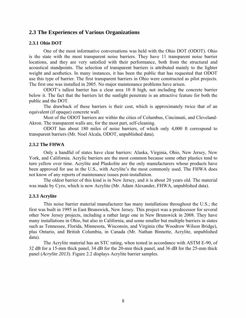
Concrete walls were already in place on the south side of the highway, both at Site 1 and Site 2; therefore, the new noise walls would be placed on top of the existing barriers to provide additional benefit to the residences. Images of the south side wall at Site 1 are presented in Figures 3.8 and 3.9.
18
Figure 3.8: South side wall on IH 30 at Site 1
Figure 3.9: South side wall on IH 30 at Site 2
3.3 Kessler Park Neighborhood
The neighborhood is just south of the highway, separated by a linear park surrounding the creek, the Coombs Creek Trail Park (Figures 3.10 and 3.11).
19
Figure 3.10: Coombs Creek Trail Park, at Site 1
Figure 3.11: Coombs Creek Trail Park, at Site 2
Kessler Parkway, a busy street that carries local traffic, runs along the park approximately parallel to IH 30; on the south side of this street are the first-row residences that are affected by the highway noise because of their proximity to it. Figure 3.12 shows an example of a first-row residence on Kessler Parkway, across the street from the park.
20
Figure 3.12: First row residence on Kessler Parkway, at Site 1
These residences are below or slightly above the highway level, but further south, the topography of the Kessler Park area is hilly, with many homes sitting at a higher elevation relative to IH 30. Figure 3.13 presents a photograph taken from a residence at much higher elevation relative to IH 30, and with clear line of sight to the highway.
Figure 3.13: View from a residence at higher elevation and clear line of sight to IH 30
21
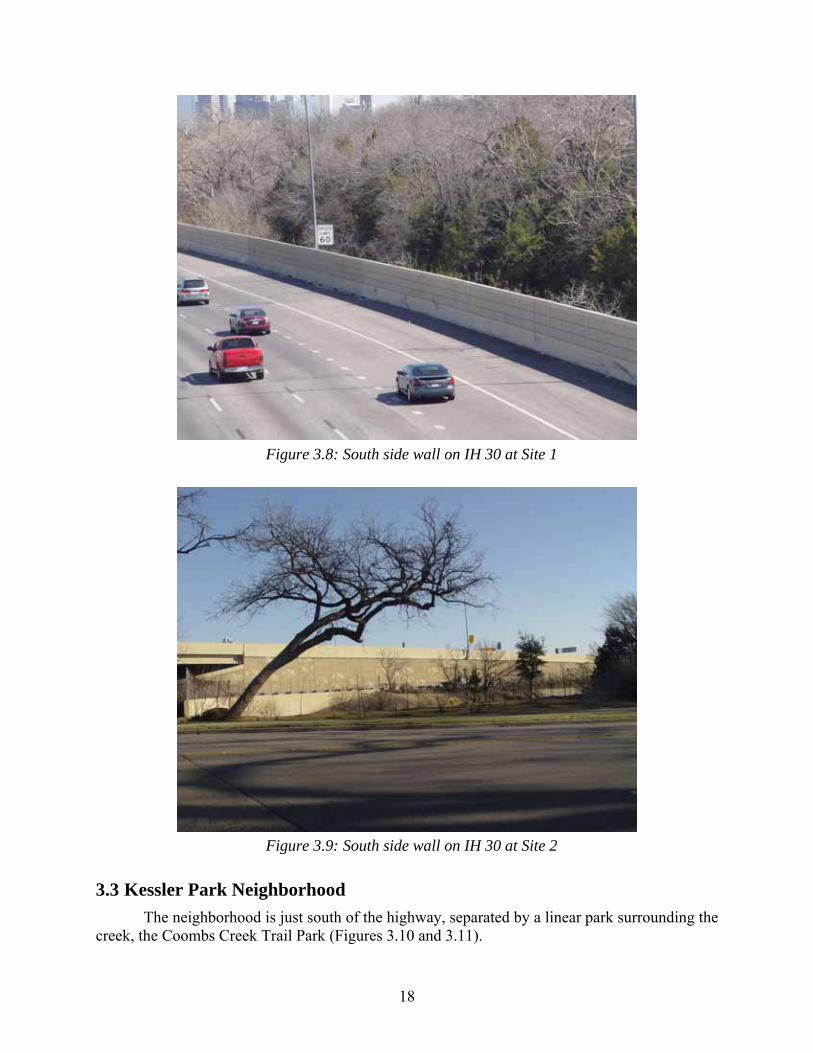
A foremost concern of the residents, as well as of TxDOT, was to preserve the views from some of the homes towards the city (Figure 3.14), and to minimize the visual impact of the highway; since the barrier would add height to the existing wall, in all likelihood, this would not be possible with an opaque barrier.
Figure 3.14: Example of a scenic view from a residence at Site 2
22
23
Chapter 4. Site 1 Barrier Design
This chapter discusses the design of the barrier corresponding to Site 1, the first stage of this project, for the elevated highway section of IH 30 between Edgefield Avenue on the west side, and Sylvan Avenue on the east side.
4.1 Introduction
A Traffic Noise Model (TNM) analysis was performed for the IH-30 Kessler Park Neighborhood in Dallas. The noise impacts were evaluated for existing and future traffic conditions. Various wall heights were analyzed to supplement the attenuation provided by the existing 8-ft wall situated on the south side of IH 30, between Edgefield Avenue and Sylvan Avenue. The analysis indicates the benefits, quantified as noise level reductions, that the various wall heights proposed are able to provide at several locations.
4.2 Receivers
Twenty-six receivers were included in the model. All of them are located between Fort Worth Avenue and Beckley Avenue Eighteen of them correspond to receivers identified in the Dallas Horseshoe Project Environmental Assessment. Also modeled were the original seven receivers identified during the 2010 and 2011 study conducted by CTR for the Dallas District (all located between Fort Worth Avenue and Sylvan Avenue), and one additional receiver on Coombs Creek Trail west of Sylvan Avenue. The Horseshoe Project receivers included the first 15 residential sites (R1 through R15), two receivers along the Coombs Creek Trail (R27 and R28), and the U.S. Post Office on the north side of IH 30 (R29).
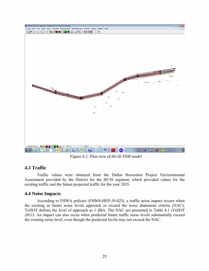
The locations of the receivers included in the TNM analysis are shown in Figure 4.1. A plan view of the model, from Hampton Road on the west to close to Beckley Avenue on the east, is shown in Figure 4.2.
24
Figure 4.1: Receivers for TNM analysis
25
Figure 4.2: Plan view of IH-30 TNM model
4.3 Traffic
Traffic values were obtained from the Dallas Horseshoe Project Environmental Assessment provided by the District for the IH-30 segment, which provided values for the existing traffic and the future projected traffic for the year 2035.
4.4 Noise Impacts
According to FHWA policies (FHWA-HEP-10-025), a traffic noise impact occurs when the existing or future noise levels approach or exceed the noise abatement criteria (NAC); TxDOT defines the level of approach as 1 dBA. The NAC are presented in Table 4.1 (TxDOT 2011). An impact can also occur when predicted future traffic noise levels substantially exceed the existing noise level, even though the predicted levels may not exceed the NAC.
26
Table 4.1: Noise abatement criteria
Thus, TxDOT policy for noise impact indicates that an outdoor residential area, such as the subject of these tests (Type B Land Use Category in Table 4.1) is considered to have an impact if the level is 66 dBA or above (TxDOT 2011).
TNM analyses were performed for both existing traffic and projected traffic. For both types of runs, an impact was identified for four receivers without additional height added to the barrier (existing wall: 8 ft). Table 4.2 shows the calculated noise levels for the future traffic for the four impacted receivers, considering only the existing 8-ft wall.
US Post Office (R29) 68.3 According to TNM, the existing wall provides a maximum of 1.4 dBA reduction for
Receiver D (not impacted), and an average reduction for all receivers of 0.3 dBA. The maximum reduction provided by the existing wall for an impacted receiver occurs for Receiver C, located along Kessler Parkway, and it is 1.1 dBA. Therefore, there are some small benefits provided by the concrete wall, but these are below a perceptible level.
4.5 Barrier Analysis
The barrier analysis was conducted for the existing 8-ft high wall, on the south side of IH 30, between Edgefield Avenue and Sylvan Avenue Additional barrier increments of 2 ft each on top of the existing wall were calculated, up to 20 ft total, i.e., new barrier heights of 2, 4, 6, 8, 10, and 12 ft on top of the existing wall.
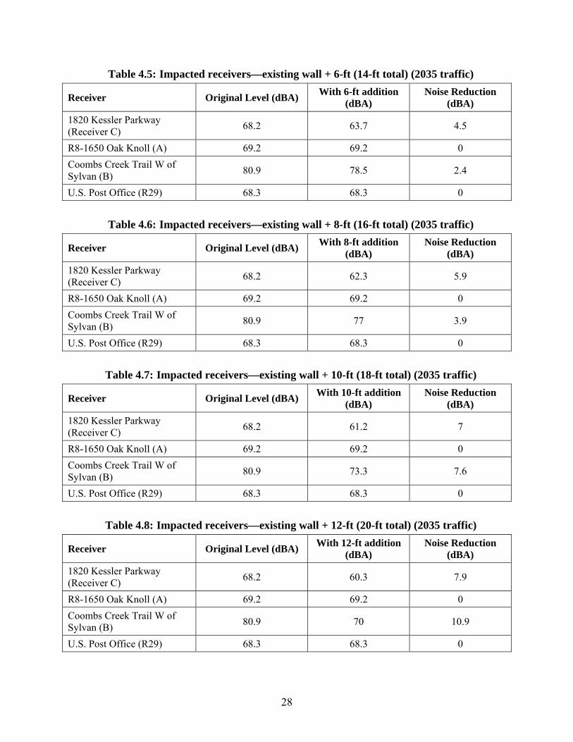
The analyses results for impacted receivers are provided in Tables 4.3 through 4.8.
The analyses show that Receiver 29, the U.S. Post Office, on the north side of the highway, as expected, does not get any benefit for any height of wall. The other receiver that is impacted that does not benefit from the wall heights analyzed in this report is Receiver 8 (also labeled as Receiver A when the initial residential measurements were performed). This residence is located at 1650 Oak Knoll, east of Sylvan Avenue. The reason this receiver does not benefit from the addition of any height to the wall is because of the site’s high elevation relative to the highway. Figure 4.3 shows a photograph taken from the residence at the time the residential measurements were performed, showing clear line of sight to IH 30, which will be difficult to block with any noise wall.
Figure 4.3: View of IH 30 from Receiver 8
Receiver C is one of the closest residential locations relative to the highway—about 250 ft from the wall in question. Figure 4.4 shows the location on 1820 Kessler Parkway. Its proximity to the highway places this receiver in the acoustical shadow of the barrier, making it the residential receiver that benefits the most from the barrier.
30
Figure 4.4: Measurements taken at Site C, on Kessler Parkway
Finally, the other impacted location is the site in the Coombs Creek Trail Park identified when the residential measurements were conducted. This site is just west of Sylvan Avenue, in close proximity to the highway as well, as shown in Figure 4.5. In the acoustical shadow of the wall, this location also benefits from any height added to the wall. This location could be representative of other sites along the park. Therefore, the park would significantly benefit from the wall’s additional height.
Figure 4.5: Measurement taken at Site B, the Coombs Creek Trail Park
31
4.6 Conclusion
The noise produced by the current and future traffic conditions creates impacts for only a limited number of receivers. Only two residences are impacted, one of which cannot receive benefit from any realistic height of wall in addition to the existing one, given its elevation relative to the highway.
The feasibility criterion indicates that the noise barrier should provide a substantial reduction, defined as a reduction of at least 5 dBA at impacted receivers. In this case, an 8-ft additional height (i.e., on top of the existing 8-ft wall for a total height of 16 ft) or higher is feasible for Receiver C, and only a 10-ft additional height or higher is feasible for Receiver B (the park). The 16-ft wall (in total height) would provide a 3.9-dBA noise reduction for locations along the park, which is a perceptible benefit.
The recommendation to the Dallas District was to install a barrier of at least 8 ft on top of the existing concrete wall, and a barrier of 10 ft if acoustic benefits were desired for the park locations. TxDOT decided to install a barrier consisting of 10-ft tall panels on top of the existing concrete at Site 1.
32
33
Chapter 5. Noise Testing Program
This chapter presents the field testing procedure conducted as part of the research work on the noise wall installation on the south side of the elevated structures on IH 30 in Dallas. The field test program consisted of noise measurements at Site 1, which is the segment between Edgefield Avenue and Sylvan Avenue, and at Site 2, which comprises the adjacent segment from Sylvan Avenue to Beckley Avenue in the vicinity of the Kessler Park neighborhood, an area which is affected by the highway noise from IH 30.
5.1 Introduction
The noise data collection took place at both Site 1 and Site 2 in the Kessler Park neighborhood before the noise wall installation at Site 1, and continued after the completion of the wall for the locations on Site 1. Five locations were monitored at each site. Measurements were performed at these locations approximately once or twice per month. During each test day, tests were conducted at all locations on three different occasions: once in the morning, once in the early afternoon, and once in the evening, to cover a wide range of traffic conditions. The purpose of the task was to gather noise data before the new sound wall was installed, to assess the noise levels prevailing at the various locations. With these measurements and subsequent measurements after the wall installation, the effectiveness of the wall can be determined. The pre-barrier condition covered a 5-month period, from the end of May to the end of October, 2013, when the barrier was completed. The post-barrier testing period started when the wall was finished and will continue through the duration of this project.
5.2 Test Equipment and Procedure
The noise measurements performed consisted of sound pressure level (SPL) tests. For these, a sound pressure meter measures the noise level over a specified time period, and the average noise level over that time period is the result of the test. The sound pressure level meter is illustrated in Figure 5.1. The time-averaged value of the sound pressure level during the test interval, i.e., the “equivalent continuous sound level” [Leq(A)] is used. Leq(A) is defined as the equivalent steady-state sound level that, in a given time period, contains the same acoustic energy as a time-varying sound level during the same period (Figure 5.2). Leq(A) is used for all traffic noise analyses for TxDOT highway projects. The meter is placed on a tripod standing 1.50 meters above the ground. Initially, the test interval was set for 15-minute periods. Because of the number of locations that needed to be tested, which included five locations at Site 1 and five locations at Site 2, and the need to gather data over the three specified times of the day (morning, early afternoon, and evening) at each one of the 10 test locations, it was impossible to measure Leq(A) for 15-minute intervals and complete all the tests necessary throughout the day, so it was decided to shorten the test intervals to 10-minute periods. Shortening the time intervals does not have any adverse effects on the test results, as the noise levels normally tend to stabilize within just a few minutes (much earlier than 10 minutes).
34
Figure 5.1: Sound pressure level meter
Figure 5.2: Leq(A): average noise level over a period of time
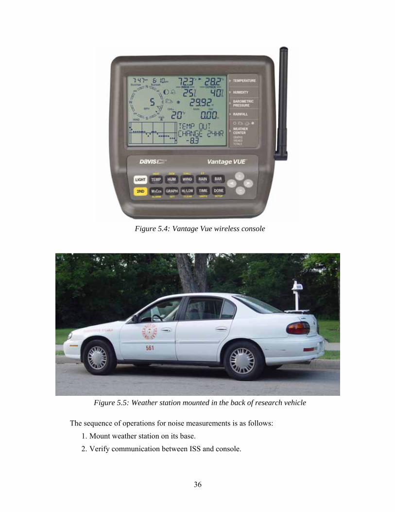
Weather conditions at the time of each test were monitored by means of a portable weather station equipped with a data logger and software. The weather station purchased for this project is manufactured by Davis Instruments and the model is called Vantage Vue (shown in Figure 5.3). It consists of an Integrated Sensor Suite (ISS) and a wireless console. The ISS contains all the sensors and devices to measure weather variables—a rain collector, temperature and humidity sensors, an anemometer, and a wind vane. It is solar-powered, and a lithium battery provides backup. It communicates wirelessly to the console by means of low-power radio transmission. The console is battery-operated and has an LCD display (Figure 5.4). The ISS measures temperature, relative humidity, dew point, wind speed, wind direction, highest wind speed (gust), gust direction, wind chill, heat index, barometric pressure, total rain, and rain rate,
(A)
EQUIVALENT NOISE LEVEL [Leq(A)]
35
and records the values for each of these variables at 1-minute intervals. Figure 5.5 shows the weather station mounted in the back of the research vehicle. The software, also created by Davis Instruments, is called WeatherLink, version 6.0.0.
Figure 5.3: Davis Instruments portable weather station, showing the ISS
36
Figure 5.4: Vantage Vue wireless console
Figure 5.5: Weather station mounted in the back of research vehicle
The sequence of operations for noise measurements is as follows:
1. Mount weather station on its base.
2. Verify communication between ISS and console.
37
3. Calibrate the SPL meter.
4. Mount the SPL meter on tripod approximately 1.2 m above the ground.
5. Level the weather station.
6. Position the weather station in such way that the solar panel faces south.
7. Start recording period. Leveling and correct orientation of the weather station must be done at each location in
order to obtain accurate wind speed and wind direction readings. Leveling is done with the aid of a bubble level on top of the ISS. A mirror compass, shown in Figure 5.6, was utilized for the orientation of the weather station. The sighting mirror in the compass allows for higher precision; its use with the weather station is shown in Figure 5.7.
Figure 5.6: Mirror compass utilized for orientation of the weather station
38
Figure 5.7: Use of the mirror compass for orientation of the weather station: the solar panel of
the weather station, in the background, is positioned so that it faces south
Steps 1 through 3 are only necessary at the beginning of a series of measurements, i.e., the beginning of each of the three recording periods (morning, early afternoon, and evening).
At the end of the day, the weather station data was downloaded from the console to the computer by means of a USB connection. The WeatherLink software facilitates analyses and graphic interpretation of weather data. Some images from the screens generated by the software are presented in Figures 5.8 and 5.9.
39
Figure 5.8: Weather plots of daily records generated by WeatherLink
40
Figure 5.9: WeatherLink screen showing weather records for every minute
5.3 Test Locations
Noise tests were conducted at ten different locations close to IH 30, five corresponding to Site 1 and five to Site 2. At each site, four locations were at residences and the fifth was in the Coombs Creek Trail Park adjacent to the highway, an area of frequent human activity. This park lies between the highway and the residences. The measurements at the homes were taken at either front patios or backyards, all outdoor places where residents would be affected by noise.
5.3.1 Site 1 Locations
Figure 5.10 maps the five Site 1 locations and the location of the noise barrier.
41
Figure 5.10: Site 1 noise measurement locations
Table 5.1 presents the addresses and coordinates for the Site 1 locations.
Table 5.1: Site 1 locations’ information
Location Address Latitude Longitude Elev. (ft)
E 2010 Kessler Parkway
N 32° 45.773’
W 96° 50.519’
434
D 1027 Evergreen N 32° 45.819’
W 96° 50.381’
505
F 1627 Nob Hill N 32° 45.887’
W 96° 50.322’
521
C 1820 Kessler Parkway
N 32° 45.896’
W 96° 50.393’
486
B
Coombs Creek Trail Park, on Kessler Parkway, west of Sylvan Avenue
N 32° 46.016’
W 96° 50.189’
458
The following paragraphs present brief descriptions of the five Site 1 locations along with
some photographs.
42
Location E
This is the residence of Ms. Sara Reidy, one of the most active neighbors from the Kessler Park Neighborhood Association in terms of her involvement with this project. The distance to the highway from this residence is 630 ft. This location is close to the highway and at a low elevation, but there is no clear line of sight to IH 30. The sound meter position at this location is in the front porch, just outside the front door, facing IH 30. Figures 5.11 and 5.12 illustrate this location.
Figure 5.11: Residential measurement at Location E
43
Figure 5.12: Residential measurement at Location E
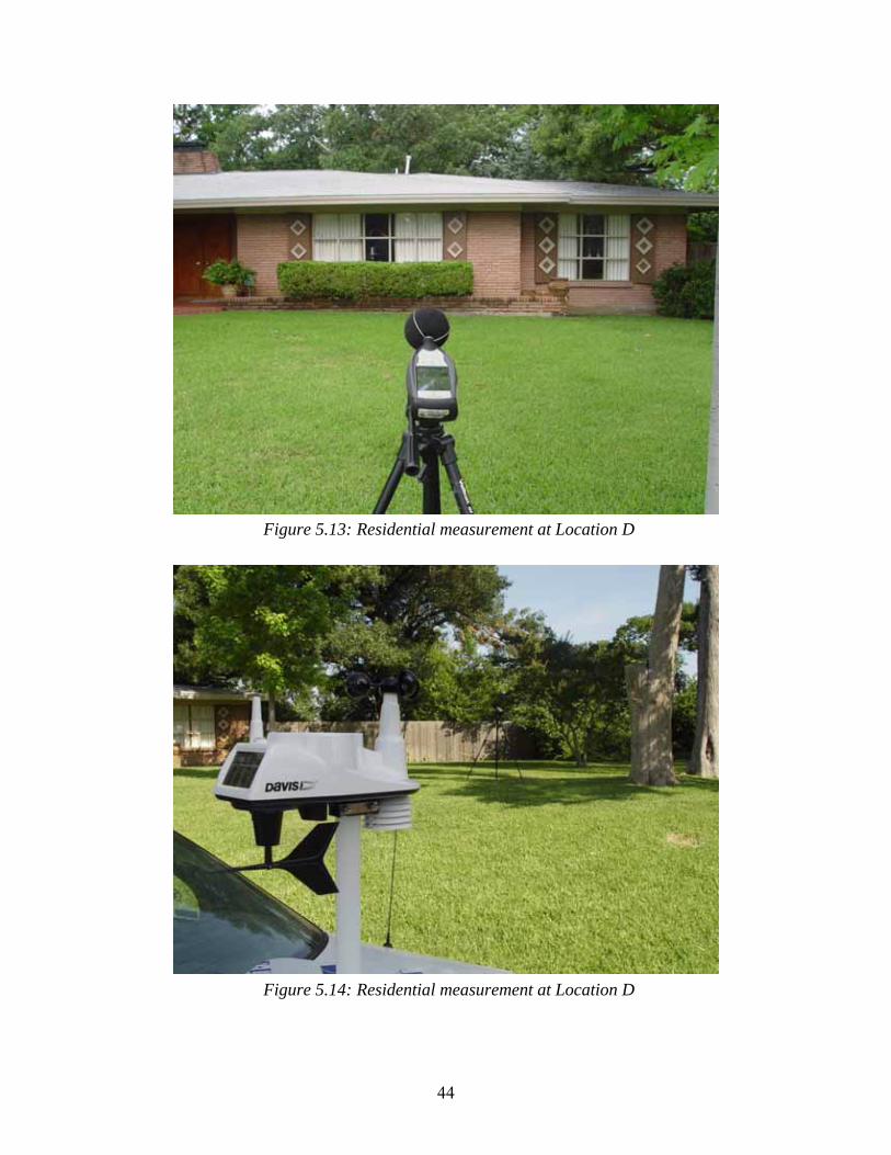
Location D
This residence is at a higher elevation and is slightly farther from IH 30. The distance to the highway is 670 ft. The measuring position at this location is in the front yard. Figures 5.13 and 5.14 show some aspects of this location.
44
Figure 5.13: Residential measurement at Location D
Figure 5.14: Residential measurement at Location D
45
Location F
This residence is at the highest elevation relative to the highway among the locations measured at Site 1. The distance to the highway is 500 ft. Figures 5.15 and 5.16 demonstrate that the street, Nob Hill, is on a steep grade, indicative of the hilly terrain just south of Kessler Parkway; the residence is to the right of the sound meter, but cannot be seen from the curb because of the dense vegetation and the steepness of the grade. The measurement position is by the curb, facing the highway.
Figure 5.15: Residential measurement at Location F
46
Figure 5.16: Residential measurement at Location F
Location C
The distance of this location to the highway is 300 ft. This residence is the closest to IH 30 among those measured. It is also slightly below the level of the highway; the only visual obstructions are vegetation and the existing concrete wall. The measurement location is at the entrance of the driveway, in front of the house (Figures 5.17 and 5.18).
Figure 5.17: Residential measurement at Location C
47
Figure 5.18: Residential measurement at Location C
Location B
This is the Site 1 location along the Coombs Trail chosen for noise measurements. It was chosen for its proximity to IH 30. The distance to the highway is 32 ft and, as Figure 5.19 shows, it is at a lower elevation relative to the highway. Coombs Creek separates this location from the highway. This location is close to Sylvan Avenue, the easternmost end of the first phase of the project. The existing concrete wall blocks the view to the highway, but the top of taller vehicles, such as trucks circulating on IH 30, can be seen from this location. This is the only location at Site 1 that offers a clear view of the wall regardless of the lushness of the vegetation. Figures 5.19 and 5.20 show measurements performed at this location before and after the barrier installation, respectively.
48
Figure 5.19: Noise measurement at Coombs Creek Trail Park (Location B) prior to noise
barrier installation
Figure 5.20: Noise measurement at Coombs Creek Trail Park (Location B) after noise barrier
installation
49
5.3.2 Site 2 Locations
Figure 5.21 maps the five Site 2 locations and the location of the proposed noise barrier.
Figure 5.21: Site 2 noise measurement locations
Table 5.2 presents the addresses and coordinates for the Site 2 locations.
Table 5.2: Site 2 locations’ information
Location Address Latitude Longitude Elev. (ft)
R3 1645 Eastus Road N 32° 45.954’
W 96° 50.042’
428
R8 1650 Oak Knoll N 32° 45.972’
W 96° 49.940’
449
R12 1126 Kessler Parkway
N 32° 46.023’
W 96° 49.827’
418
R13 1060 Kessler Parkway
N 32° 45.961’
W 96° 49.797’
465
R27
Coombs Creek Trail Park, on Kessler Parkway, east of Sylvan Avenue
N 32° 46.020’
W 96° 49.756' 418
50
The following paragraphs present brief descriptions of the five Site 2 locations along with some photographs.
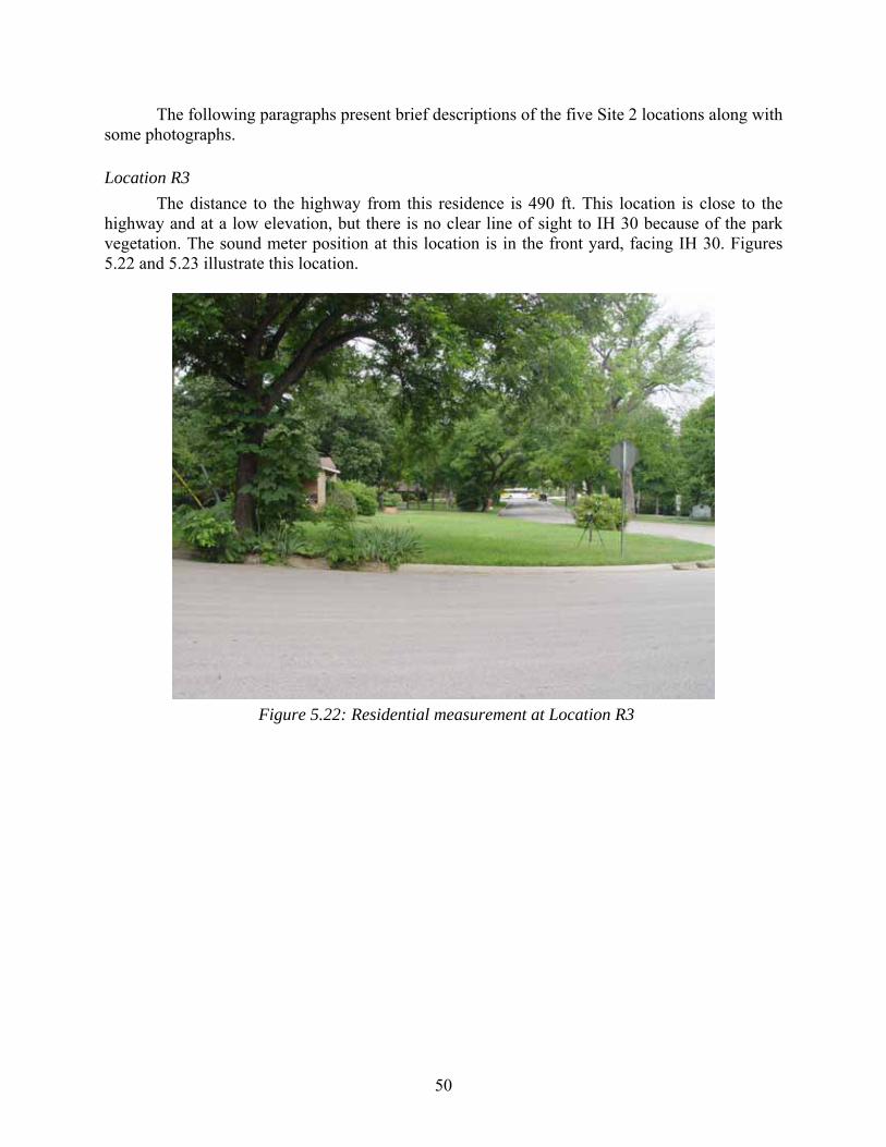
Location R3
The distance to the highway from this residence is 490 ft. This location is close to the highway and at a low elevation, but there is no clear line of sight to IH 30 because of the park vegetation. The sound meter position at this location is in the front yard, facing IH 30. Figures 5.22 and 5.23 illustrate this location.
Figure 5.22: Residential measurement at Location R3
51
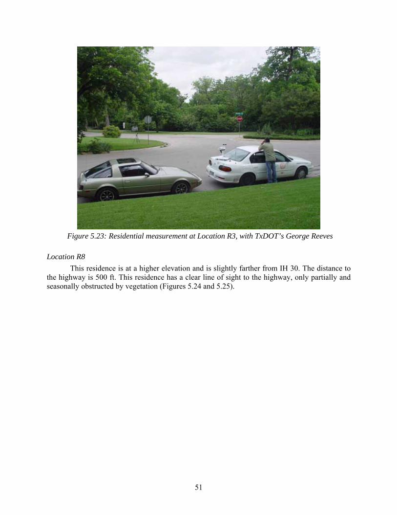
Figure 5.23: Residential measurement at Location R3, with TxDOT’s George Reeves
Location R8
This residence is at a higher elevation and is slightly farther from IH 30. The distance to the highway is 500 ft. This residence has a clear line of sight to the highway, only partially and seasonally obstructed by vegetation (Figures 5.24 and 5.25).
52
Figure 5.24: Residential measurement at Location R8
Figure 5.25: IH-30 view from residence at Location R8
53
Location R12
This residence is at the lowest elevation relative to the highway among the locations measured at Site 2. It is also the closest to IH 30. The distance to the highway is 280 ft. It is just across the street from the Coombs Creek Trail Park. The measurement position is in the front yard, close to the curb, facing the highway (Figures 5.26 and 5.27).
Figure 5.26: Residential measurement at Location R12
54
Figure 5.27: Residential measurement at Location R12
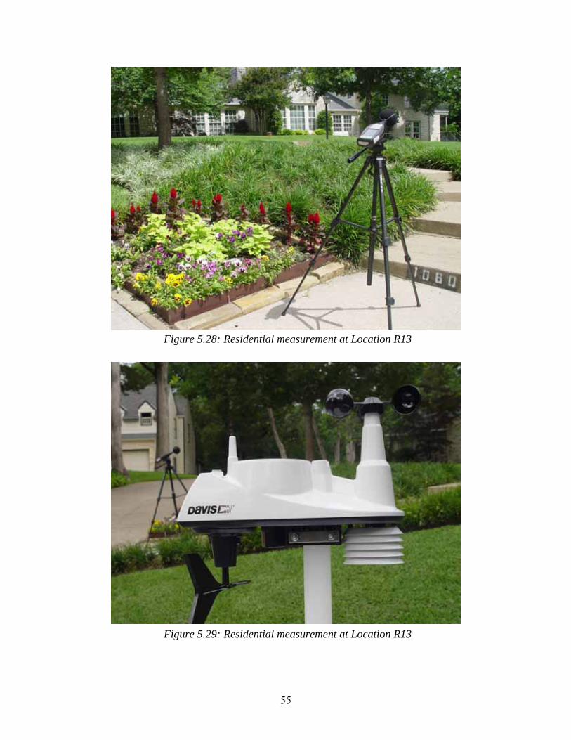
Location R13
This is the furthest location from the highway, among the Site 2 locations. The distance of this location to the highway is 675 ft. It is also at the highest elevation from the highway, as Kessler Parkway is in a steep incline as it turns south, away from IH 30. The measurement location is in the front yard, on the steps leading to the entrance of the house (Figures 5.28 and 5.29).
55
Figure 5.28: Residential measurement at Location R13
Figure 5.29: Residential measurement at Location R13
56
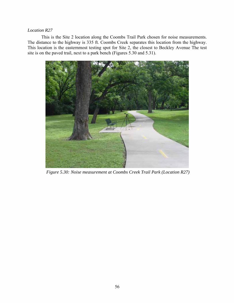
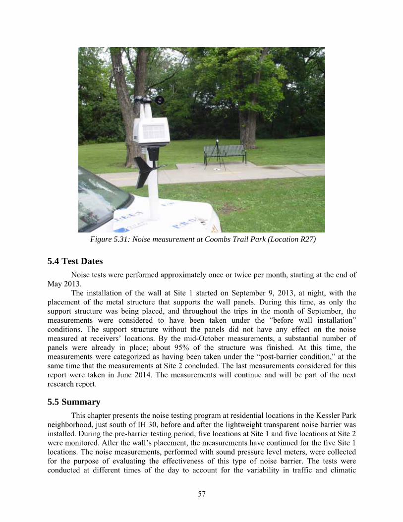
Location R27
This is the Site 2 location along the Coombs Trail Park chosen for noise measurements. The distance to the highway is 335 ft. Coombs Creek separates this location from the highway. This location is the easternmost testing spot for Site 2, the closest to Beckley Avenue The test site is on the paved trail, next to a park bench (Figures 5.30 and 5.31).
Figure 5.30: Noise measurement at Coombs Creek Trail Park (Location R27)
57
Figure 5.31: Noise measurement at Coombs Trail Park (Location R27)
5.4 Test Dates
Noise tests were performed approximately once or twice per month, starting at the end of May 2013.
The installation of the wall at Site 1 started on September 9, 2013, at night, with the placement of the metal structure that supports the wall panels. During this time, as only the support structure was being placed, and throughout the trips in the month of September, the measurements were considered to have been taken under the “before wall installation” conditions. The support structure without the panels did not have any effect on the noise measured at receivers’ locations. By the mid-October measurements, a substantial number of panels were already in place; about 95% of the structure was finished. At this time, the measurements were categorized as having been taken under the “post-barrier condition,” at the same time that the measurements at Site 2 concluded. The last measurements considered for this report were taken in June 2014. The measurements will continue and will be part of the next research report.
5.5 Summary
This chapter presents the noise testing program at residential locations in the Kessler Park neighborhood, just south of IH 30, before and after the lightweight transparent noise barrier was installed. During the pre-barrier testing period, five locations at Site 1 and five locations at Site 2 were monitored. After the wall’s placement, the measurements have continued for the five Site 1 locations. The noise measurements, performed with sound pressure level meters, were collected for the purpose of evaluating the effectiveness of this type of noise barrier. The tests were conducted at different times of the day to account for the variability in traffic and climatic
58
conditions. At the same time the noise tests were performed, a weather station was used to monitor climatic variables. A detailed description of the equipment utilized for the measurements was presented, as well as the methodology for the field work.
59
Chapter 6. Test Results and Analysis
This chapter presents the data processing, results, and analysis of the noise data collected as part of the research work conducted before and after the noise wall installation on the south side of the elevated structures on IH 30 in Dallas.
The work consisted of organizing and analyzing the noise and weather data collected for about a year in the vicinity of the Kessler Park neighborhood, an area affected by the highway noise from IH 30. The noise and weather data corresponds to both Site 1 and Site 2. Site 1 is the segment between Edgefield Avenue and Sylvan Avenue, south of the highway, and Site 2 corresponds to the area between Sylvan Avenue and Beckley Avenue, also south of IH 30, just west of downtown Dallas. The data analyzed was gathered at both Site 1 and Site 2 for the pre-barrier condition, and at Site 1 for the post-barrier condition.
6.1 Analysis of Overall Results and TNM Predictions
There were 260 noise measurements taken before the wall was installed (130 at Site 1, 130 at Site 2), and 125 noise measurements taken after wall was installed (at Site 1 only). About 4,000 weather records (one every minute) were collected while the noise tests took place.
Following are the average noise measurements for both sites, before and after the wall was installed:
Average level before wall, Site 1: 58.2 dBA Average level after wall, Site 1: 56.6 dBA Average level before wall, Site 2: 58.2 dBA Therefore, before the noise wall was installed, the noise measurements were similar at
both Site 1 and Site 2; and Site 1 showed a 1.6 dBA reduction, on average, after the wall was installed. The following section presents the analysis of the measurements, including comparisons with the design program’s predictions.
6.1.1 Site 1
Unlike at Site 2, Site 1 noise measurements continued after the installation of the noise wall was completed. Figure 6.1 shows average before and after noise wall average measurements by location for Site 1.
60
Figure 6.1: Site 1 average noise measurements, before and after noise wall installation
All the locations at Site 1 show some small benefit, on average, from the noise wall. The location with the smallest average benefit is location E (0.7 dBA), the westernmost residential location, which is very close to the west end of the noise wall, at Edgefield Avenue In all likelihood, highway noise coming from west of Edgefield Avenue still reaches this residence and this could be the reason for the marginal noise reduction after the wall was installed. The location with the highest average noise reduction after the wall was in place is residence C, the closest residence to the highway. This location shows a 2.5 dBA average noise reduction with the noise wall. Besides its proximity to the highway, this location is at a lower elevation relative to the highway, which results in higher benefit from the wall. Another location that is very close to the highway, and at a lower elevation, is the park location, identified as B; its benefit, on average, is 1.0 dBA. It would be expected that this location would obtain a greater noise reduction from the wall, but some of that benefit might be negated by its proximity to the easternmost end of the wall, at Sylvan Avenue—noise from the highway segment not protected by the wall still reaches this park location, as is the case with location E, at the other end of the project.
For the design of the noise wall, the TNM program was utilized, as described in Chapter 4. The comparison of the results, before and after, with the TNM predictions is shown in Figure 6.2. The TNM predictions correspond to two levels of traffic, the current and the future (year 2035) traffic, which was used as an input for the wall’s design.
61
Figure 6.2: Site 1 average noise measurements, before and after noise wall installation,
compared with TNM predictions
The TNM predicts substantial reductions for the 2035 traffic at all locations shown in Figure 6.2 when comparing the no-wall condition to the wall condition, except for location E, where the benefit is only 0.5 dBA, according to the prediction. According to the program, the highest benefit for these traffic levels would be achieved at location B (7.6 dBA), with location C following closely (7.0 dBA). In regards to the comparisons between actual measurements and TNM predictions, the program over-predicts in four of the locations—in three of them by a wide margin—and it under-predicts for location E. The largest over-prediction is for location B, about 7 or 8 dBA, depending on whether the comparison is before or after the wall installation.
Site 1 Existing Concrete Wall Noise Reduction Contribution
TNM runs with and without the existing 8-ft. concrete wall show that the maximum benefit provided by the concrete wall itself accounts for 1.4 dBA. This number indicates that the concrete wall already provides a small benefit, and helps clarify the magnitude of the contribution of the new transparent wall. Therefore, the residences at Site 1 get the benefit of having the concrete wall in addition to the transparent wall.
6.1.2 Site 2
Measurements at Site 2 concluded at the time the noise wall installation was completed (mid-October 2013). Figure 6.3 shows the average measurements by location at Site 2.
62
Figure 6.3: Site 2 average noise measurements, before noise wall installation
The comparisons between the TNM program’s predictions and actual results are shown in Figure 6.4. This figure presents a comparison of the actual measurements and the TNM predictions for the current traffic and the future (year 2035) traffic.
Figure 6.4: Site 2 average noise measurements, before noise wall installation, compared with
TNM predictions
TNM over-predicted noise levels for four of the five locations corresponding to Site 2. The average over-prediction is 5.05 dBA. However, this number is inflated by the result at one location, R8, where the program’s over-prediction is 11.1 dBA. For receiver R12, the only one for which TNM under-predicted the noise level, the under-prediction is 2.8 dBA. Also, the
63
TNM-predicted noise levels at the current level of traffic are very similar to those predicted for the future traffic.
6.2 Analysis of Measurements
In this section, the noise results are analyzed by date, and in relationship to the weather variables.
6.2.1 By Test Date
Noise levels were fairly consistent before the noise wall was installed, from May 2013 to mid-October 2013. After the noise wall was finalized, the trend of the noise measurements went down, but in the winter months, the noise levels seemed to get higher again. Since the weather turned warm and then rather hot, noise levels have been fairly low, on average, for the locations in Site 1. These trends indicate the high influence of seasonal changes on the noise levels. A chart showing total averages for measurements by date, for both Site 1 and Site 2, is shown in Figure 6.5.
Figure 6.5: Average noise levels by date
There has been much more variability in the measurements after the wall was installed, i.e., dating from the October 28, 2013, measurements and after.
Temperature
The most important contribution of a weather variable to the seasonal variation of noise is the effects of temperature. To further analyze the seasonal variations of noise that occurred after the wall was installed, the plot shown in Figure 6.6 was prepared for the Site 1 locations. In this plot, the noise levels before the wall was installed are averaged, and then compared to the variations in levels by date after the wall was completed for each of the Site 1 locations. This graph confirms that the February 2014 measurements were slightly louder for all locations. Cold
64
temperatures are correlated to higher tire-pavement noise generation (1 dBA per 10°C) (Sandberg 2002). Therefore, for instance, a change from a temperature of 95°F, typical for the summer in Dallas, to a temperature of 40°F, which is very common in the winter, represents an increase of 3 dBA in tire-pavement noise generation alone, with all the other conditions staying constant. Such a difference in noise levels, attributable to temperature change only, represents a significant increase. In general, under colder conditions, the pavement materials as well as the rubber in the tires are stiffer and produce higher noise levels than during warmer conditions.
Figure 6.6: Noise levels before and after wall, for Site 1 locations
This graph also shows that location B, the Coombs park measuring spot, as well as location C, are consistently the loudest locations due to their proximity to the highway. Similarly, location D is consistently the quietest as it is farther away from the highway.
The relationship between noise measurements and air temperature was investigated in Figure 6.7, which includes both Site 1 and Site 2 tests, before and after the noise wall was installed. As mentioned in the previous section, the measurements were more consistent and less scattered before the wall was in place, whereas the variability increased in the measurements after the wall was installed. It is very noticeable that all of the measurements before the wall installation were taken in warm temperatures, between 70 and 110 °F, while most of the measurements after the installation correspond to temperatures between 25 and 70 °F, with only a few measurements taking place when temperatures were above 80 °F.
The average temperature for the tests before the barrier was 90.1 °F, with an average noise level of 58.2 dBA, whereas for the post-barrier tests, the average temperature was 66.0 °F, with an average noise level of 56.6 dBA. This indicates that, in spite of the high temperature differential, the barrier is still providing important benefits. A flaw of this data set is that there were no tests conducted in cold weather for the pre-barrier condition. The assumption is that the noise levels for cold weather conditions before the barrier would have been much higher than 58.2 dBA, and this would have made the barrier’s benefit more obvious.
65
Figure 6.7: Noise level and temperature
The statistics for temperature and noise levels are shown comparatively in Table 6.1, for measurements before and after the wall installation. It is interesting to note the variability of the temperature and noise levels, especially after the wall was installed.
Table 6.1: Statistics for temperature and noise level
Before Wall (Site 1 and
Site 2) After Wall (Site 1)
Temperature
(°F) Leq
(dBA) Temperature
(°F) Leq
(dBA)
Mean 90.1 58.2 66.0 56.6
Standard Deviation 7.2 3.2 19.3 3.9
Median 91.2 57.8 72.4 56.3
Mode 83.0 56.4 74.8 55.8
C.V. (%) 8.0 5.5 29.2 6.9
Minimum 70.0 49.1 26.4 49.4
Maximum 103.3 64.5 93.7 66.5
Range 33.3 15.4 67.3 17.1
Count 260 260 125 125
66
Wind
The wind and its direction were expected to be important factors in the noise levels. One main reason for monitoring the wind was that, according to residents’ accounts, the noise problem was exacerbated by strong winds blowing from the north and carrying the noise from the highway towards the residential area. However, the large amount of data collected at the various locations does not confirm this hypothesis. Neither the average wind speed nor the higher wind speeds (gusts) provide a strong correlation with noise levels. Figure 6.8 shows a plot of noise levels and wind speed, in which each data point corresponds to a noise measurement and the average wind speed that was obtained by the weather station during the noise measurement. It shows both before and after noise wall measurements and the two weak correlations do not indicate that higher noise levels occurred with higher winds, but rather, the opposite. Similarly, Figure 6.9 presents the relationship between noise levels and high wind speeds (gusts), showing a poor correlation as well, indicating no influence of the gusts on noise levels measured at the neighborhood.
Figure 6.8: Noise level and average wind speed
67
Figure 6.9: Noise level and high wind speed
Wind Direction
For the wind direction analysis, given that throughout each test period for an individual test (normally 10 minutes) the wind direction commonly fluctuates, the dominant wind direction for each test is considered to be that of the highest gust within that period. Therefore, for each test there is an average noise level, an average wind speed, a high wind speed (gust), and a high wind direction. The average wind speed is a scalar, whereas the gust is a vector.
The results are grouped in three categories:
1. Site 1-before the barrier
2. Site 1-after the barrier
3. Site 2 The results of the wind direction analysis are shown in a group of four charts. The first
chart (labeled as “a”) shows the percentage of the tests associated with each wind direction. In the second chart (b), the average noise levels were plotted with the wind direction of the gust as well as the gust speed. Finally, in the third (c) and fourth (d), the gust levels were plotted against the average noise levels, with (c) showing the values for each wind direction, and (d) showing the correlation. Therefore, the data points for (c) and (d) are identical.
The charts are shown in Figures 6.10, 6.11, and 6.12, for Site 1-before the barrier, Site 1-after the barrier, and Site 2, respectively.
68
Figure 6.10: Site 1 before barrier: a) Dominant wind direction by percentage of time; b)
Average noise levels and average gusts by direction; c) Average noise level vs. average gust by direction; and d) Average noise level and average gust correlation
For Site 1 in the pre-barrier condition, the majority of the time (16%) the gusts blew from the SW direction, with the SSW being the second most dominant gust direction (15%). However, the highest average noise level (61.1 dBA) occurred when the gusts blew from the WSW direction. The correlation between gust speeds and average noise levels is very poor and shows that louder noise levels happened with lower gusts, and vice versa.
69
Figure 6.11: Site 1 after barrier: a) Dominant wind direction by percentage of time; b) Average
noise levels and average gusts by direction; c) Average noise level vs. average gust by direction; and d) Average noise level and average gust correlation
For Site 1 in the post-barrier condition, the most dominant gust direction was NNE (14%). However the highest average noise level (59.1 dBA) occurred when the gusts blew from the SW direction. The correlation between gust speeds and average noise levels is also very weak and shows that louder noise levels happened with lower gusts, and vice versa.
70
Figure 6.12: Site 2: a) Dominant wind direction by percentage of time; b) Average noise levels
and average gusts by direction; c) Average noise level vs. average gust by direction; and d) Average noise level and average gust correlation
Finally, for Site 2 there is only the pre-barrier condition. Site 2 shows some positive correlation between gusts and noise levels, indicating that the higher gust speeds corresponded with higher noise levels. The dominant wind direction was SW (12%), followed closely by the SSW (11%). The higher average noise levels (59.2 dBA) occurred when the gusts blew from the NE. However, the distribution of average noise levels is very even among the eleven other wind directions, while corresponding average noise levels are in the range of 57 to 59 dBA.
Relative Humidity
The measurements for relative humidity were fairly uniform for the pre- and post-barrier conditions. The mean value was 50% for the pre-barrier measurements and 58% for the post-barrier tests. The correlation with noise levels in both cases is negligible (Figure 6.13) and very similar, showing that this weather variable had no influence on the noise measurements.
71
Figure 6.13: Noise level and relative humidity
Table 6.2 summarizes the analysis of weather variables, presenting the descriptive statistics.
Table 6.2: Statistics for weather variables and noise level
6.2.2 Pre- and Post-Barrier Analysis
t-test
One way to analyze the barrier’s effectiveness is by comparing before and after noise levels and determining whether the differences between the pre-and post-barrier conditions are significant. A t-test is used to determine if two sets of data are significantly different from each other. The test assumes that the variables being studied—in this case, measured noise levels—follow a normal distribution. The distribution of measured noise levels for both the pre- and post-barrier for Site 1 tests are shown in Figure 6.14.
Before Wall (Site 1 and Site 2) After Wall (Site 1)
72
Figure 6.14: Frequency distribution for pre-barrier (a) and post-barrier (b) tests
A two-sample t-test was performed, with independent (unpaired) samples; the assumptions were equal variances, α=0.05, and a two-tailed distribution. The null hypothesis in this case is that the barrier had no effect on the measured noise levels, and the alternative hypothesis is that the barrier had an effect. If the difference between these distributions is large enough, the null hypothesis would be rejected.
Table 5 shows the results. The row containing the probability for the t-tests (p-value) is the second to last, and it has been highlighted in red. If the p-value is less than the significance level α, the difference in noise levels between the groups being compared is considered statistically significant, as it was the case for the pre- and post-barrier noise tests for Site 1. Therefore, the null hypothesis was rejected, indicating that there was a statistically significant difference between the groups of tests; hence, the t-test supports the measurements indicating that the barrier had indeed an effect on noise levels.
Table 6.3: Statistics for weather variables and noise level
Spectral Differences
The noise data was analyzed in one-third octave band spectra averaged throughout the pre- and post-barrier testing periods for each location. This analysis illustrates the distribution of noise levels before and after the barrier, among the different frequencies. The graphs for Site 1 are shown in Figure 6.15. These data show that Location C—the site with the greatest acoustic benefit from the barrier, but also the loudest one with and without barrier—has higher noise
Before After Mean (dBA) 58.2 56.6Variance 12.588 15.484 Observations 130 125 Pooled Variance 14.007 t Stat 3.320 P(T<=t) 0.001 t Critical 1.969
73
levels at the lower frequencies, much more than any other location, by a wide margin. This is due perhaps to the location’s close proximity to the highway; and with the barrier, this location gets important reduction in the frequencies between 400 and 1250 Hz. Locations D and F, the more distant sites from the highway, have flatter spectra and lower levels.
Figure 6.15: Average frequency spectra for Site 1 locations for pre-barrier and post-barrier
tests
6.3 Summary and Discussion of Results
This chapter presents the data analysis for before and after the barrier conditions for Site 1, and for the pre-barrier condition for Site 2. The measurements analyzed include tests conducted from May 2013 until June 2014. The tests show that all locations on Site 1 have received some benefit from the noise wall. Although the average benefits seem acoustically
74
small for most locations, the t-test showed that they are statistically significant, confirming that the barrier has had an effect on noise levels.
Seasonal changes—primarily temperature—seemed to have a definitive influence on the noise levels. The sound barrier provided higher noise reduction in the few months following its completion, while the weather was still warm. It is well documented that cold temperatures are correlated to higher tire/pavement noise generation.
Noise levels got very high in the colder months, and decreased again in the months of May and June 2014, during which weather conditions were very hot. Therefore, when averaging all results, the benefits seem small.
75
Chapter 7. Monitoring
This chapter presents the results of field inspections performed at Site 1’s new transparent sound wall, as part of the research work conducted on the elevated highway structure on IH 30 in Dallas. The work consisted of periodic monitoring of the wall, which extends from Edgefield Avenue to Sylvan Avenue, in the vicinity of the Kessler Park neighborhood, an area affected by the highway noise from IH 30. This work started when the Site 1 noise barrier installation began, and has continued after the wall’s completion; this chapter covers the monitoring activities until the most recent visit in July 2014.
This work consisted of monitoring the condition and maintenance status of the completed Site 1 sound wall at monthly intervals. Monitoring activities consist of visual inspection of the wall, documenting its status, and photographing visible defects. The research team documented any special measures needed following physical damage to the lightweight barriers after the noise wall installation and reported any damages or defects to the District personnel.
7.1 Sound Wall Installation
The noise barrier installation on IH 30 in Dallas for the segment between Edgefield Avenue and Sylvan Avenue, began in September 2013, and it concluded by mid-October 2013. The wall consists of transparent acrylic panels, made of a material called Acrylite, manufactured by Evonic, which are 15-mm thick, 7-ft wide by 10-ft tall, placed on top of the existing 8-ft tall concrete barrier on the south side of IH 30. Some panels are narrower to allow for the expansion joints of the elevated structure; those are 4-ft-wide instead of 7-ft-wide. Also, at the easternmost end of the barrier, over Sylvan Avenue, the last few panels are 13-ft tall, as the existing concrete barrier is shorter. The total length of the wall is 2,395 ft.
The project was bid at $885,000. With a surface area of 23,950 sq ft, the cost per unit area is approximately $37/sq ft. The bid tabulations for the job show the cost per unit area for the winning bidder to be $35.89/sq ft because the bid did not account for traffic control, barricades, etc.
The installation took place at night (Figures 7.1 and 7.2). Work required one-lane closures between 10:00 p.m. and 6:00 a.m. only. The contractor performing the installation was Highway Intelligent Traffic Solutions, Inc., and the transparent material and structural design for the wall were provided by Armtec.
76
Figure 7.1: Nighttime installation
Figure 7.2: Vertical support placement
Some images of the completed wall are shown in Figures 7.3 to 7.8.
77
Figure 7.3: Sound wall as seen from Edgefield Avenue Bridge
Figure 7.4: Sound wall as seen from Edgefield Avenue Bridge
78
Figure 7.5: Sound wall as seen from Edgefield Avenue Bridge
Figure 7.6: Sound wall as seen from westbound IH 30
79
Figure 7.7: Sound wall as seen from westbound IH 30 looking towards Edgefield Avenue
Bridge
Figure 7.8: Sound wall as seen from westbound lanes looking towards downtown
A few problems were noticed before the completion of the installation, such as some
supports not being completely vertical (Figures 7.9 and 7.10), some apparently missing rubber gaskets between panels and the metal supports, some gaskets slightly out of place (Figure 7.11), as well as some gaps between gaskets and metal supports, both for vertical and horizontal gaskets (Figures 7.12 and 7.13).
80
Figure 7.9: Some vertical supports off-plumb
Figure 7.10: Vertical support off-plumb
81
Figure 7.11: Gasket shown protruding from metal support
82
Figure 7.12: Gap between vertical gasket and metal support
Figure 7.13: Gap between horizontal gasket and metal support
83
CTR spoke with Mr. Mark McIlheran, P.E., structural engineer from Armtec, about some of these defects. He suggested CTR meet with him and Mr. George Reeves, from TxDOT, to inspect the wall so that CTR could show the location of some of these issues. On October 28, Manuel Trevino, with CTR, met with Mr. McIlheran and Mr. Reeves at the site (Figure 7.14) and inspected the wall, both from the Edgefield Avenue Bridge and walking along the wall from the eastbound-side shoulder of IH 30. Mr. McIlheran said he would contact the contractor, Highway Intelligent Traffic Solutions, to fix the off-plumb posts, the gaskets that are apparently missing or out of place, and a panel that is warping because the vertical supports are too tight and off-plumb for one of the spans of the wall.
Figure 7.14: Armtec’s Mark McIlheran inspecting the wall, showing the gap size between a
panel and the gasket
Additionally, some gaps were observed in the existing concrete wall at the expansion joints of the bridge (Figures 7.15 and 7.16), gaps that should be filled with some elastic joint sealing material allowing for the bridge’s thermal expansion and contraction. Such material should prevent the sound from traveling from the highway to the neighborhood to further attenuate the noise at the receivers’ locations and contribute to the wall’s effectiveness. This would be TxDOT’s responsibility, as it is not an issue of the transparent noise wall, but rather of the existing structure.
The gaps between gaskets and frames and the gaps in the concrete wall are important elements of concern in regards to the acoustical performance of the wall, as any opening will hinder the wall’s effectiveness.
84
Figure 7.15: Gap in existing concrete wall at bridge expansion joint as seen from Coombs
Creek
Figure 7.16: Gap in existing concrete wall at bridge expansion joint as seen from the highway
side
7.2 Graffiti
On November 11, 2013, while performing the wall inspection, it was noticed that some of the panels had been damaged by graffiti. Ten transparent panels, from spans # 135 to 144 (as marked by the contractor on the concrete wall during installation) were sprayed. The concrete wall under span # 144 was also painted. From the distance, the damage was barely noticeable, and from some angles, it was not visible at all. The appearance of the sprayed material was that
85
of some type of drywall mud or acoustic texture that is used in ceilings. Pictures of the graffiti are shown in Figures 7.17 to 7.23. The damage was reported immediately to TxDOT.
Figure 7.17: Graffiti as seen from the highway shoulder on November 11, 2013
Figure 7.18: Graffiti as seen from the highway shoulder on November 11, 2013
86
Figure 7.19: Graffiti as seen from the highway shoulder on November 11, 2013. The damage
extends to the concrete wall under span #144.
Figure 7.20: Graffiti as seen from the highway shoulder on November 11, 2013
87
Figure 7.21: Graffiti as seen from the highway shoulder on November 11, 2013
Figure 7.22: Graffiti seen from the north side of IH 30
88
Figure 7.23: Graffiti seen from the north side of IH 30
During the remaining part of November and December 2013, no work was performed to clean the sound wall. By January 28, 2014, the panels had been cleaned. The following cost information for the cleaning operations was kindly provided by Mr. Frank Jett, with the Dallas District, Heavy Equipment Maintenance:
Traffic Control: $3,893.27 Steam Cleaner: $200.00 Graffiti Removal: $73.50 Total: $4,166.77 The following photographs illustrate the appearance of the cleaned acrylic panels during
the January 28, 2014 site visit (Figures 7.24 and 7.25).
89
Figure 7.24: Cleaned panel showing traces of the cleaning operation
Figure 7.25: Cleaned panel showing traces of the cleaning operation
Figure 7.26 shows that the graffiti that extended to the concrete wall could not be entirely removed, and Figure 7.27 shows a photograph taken from afar after the panels had been cleaned.
90
Figure 7.26: Remnants of the graffiti on the concrete wall below the panels
Figure 7.27: Graffiti removed from acrylic panels
7.3 Gasket Deterioration and Openings
Besides the graffiti, which was successfully removed, the main problem with the wall has been the deteriorating condition of the rubber gaskets that are supposed to seal the spaces between panels and the metal supports and the existing concrete walls. This problem was reported shortly after the wall was installed, as it was detected in the inspections during the installation as mentioned before in this document. In the subsequent months, the condition of such gaskets appeared to worsen. Many of the gaskets were not properly placed from the time the wall was installed, and now, perhaps due to the weather, some of them are falling out of place, sagging and
91
even breaking, leaving open gaps through which the noise travels from the highway to the neighborhood. Making an analogy with architectural acoustics, this is similar to leaving an opening (e.g., an open window or a gap under a door) in a room, in which case the acoustic energy goes through the opening, and the transmission loss of the walls is undermined by the area of the opening, significantly reducing the transmission loss of the wall. The problem with the gaskets occurs in both the vertical and horizontal gaskets, but the worst cases correspond to the horizontal gaskets that seal the bottom of the acrylic panels with the concrete wall. The sagging of the horizontal gaskets can be seen in Figures 7.28 through 7.31.
Figure 7.28: Sagging of horizontal rubber gaskets
Figure 7.29: Sagging of horizontal rubber gaskets
92
Figure 7.30: Sagging of horizontal rubber gaskets
Figure 7.31: Sagging of horizontal rubber gaskets
Some of the gaskets have broken, as shown in Figures 7.32, 7.33, and 7.34.
93
Figure 7.32: Broken horizontal rubber gasket
Figure 7.33: Broken horizontal rubber gasket
94
Figure 7.34: Broken horizontal rubber gasket
In some cases, the vegetation from the creek side grows through the openings in the gaskets and gets in front of the panels on the highway side, illustrating how widespread the problem has become (Figures 7.35 and 7.36).
Figure 7.35: Vegetation from the creek side growing through the openings in the gaskets under
noise barrier
95
Figure 7.36: Vegetation from the creek side growing through the openings in the gaskets under
noise barrier
In May 2014, CTR learned that the contractor had offered to fix the problems with the gaskets at no cost to TxDOT. As of the latest monitoring visit to the barrier on July 11, 2014 (prior to the finalizing this document), no repairs had been made to the gaskets. It is estimated that about 80% of the horizontal gaskets are in poor condition (broken, sagging, or out of place), which significantly hinders the acoustic performance of the barrier.
Another problem not directly related to the acrylic wall, but one that minimizes its effectiveness, is the high number of open joints in the existing concrete wall. This was mentioned before in this document, as it was noticed shortly after installation of the wall had been completed. These gaps are as wide as 3 or 4 in. (Figure 7.37); the joint sealants are old and have disintegrated with time and weather (Figure 7.38), allowing the acoustic energy to travel to the neighborhood. The vegetation is also growing through these gaps, as can be seen Figure 7.39. If these can be sealed and the gaskets can be repaired, the wall could be much more effective in mitigating the noise.
96
Figure 7.37: Expansion joint opening due to lack of sealant
97
Figure 7.38: Damaged, old sealant material in the expansion joints of bridge structure
98
Figure 7.39: Vegetation from the creek side growing through the openings in the concrete
structure
7.4 Summary
This chapter presents the results of the monitoring activities of the new lightweight transparent noise barrier on the south side of IH 30, in the area delimited by Edgefield Avenue in the west, and Sylvan Avenue in the east, starting with its installation and continuing through its subsequent service life, including periodic inspections and documentation of condition. The main issues identified so far are the following:
• Some of the vertical metal posts of the support structure off-plumb
• Gaskets sealing the joints between posts and panels not properly installed
• Gaskets sagging and even breaking as a result of faulty initial placement and weather
• An occurrence of vandalism: graffiti temporarily damaged 10 panels, but was removed by maintenance crews without further consequences
• Openings in concrete bridge structure expansion joints without sealant or gaskets that allow sound to travel from highway to receivers
99
Chapter 8. Conclusions and Recommendations
This chapter presents the preliminary conclusions of the study, 18 months after project initiation. This research project investigated the feasibility of a lightweight noise barrier on IH 30 in Dallas. An investigation of lightweight and transparent materials for noise barriers was conducted, gathering information from the literature and the experiences of other DOTs and organizations, including vendors and material manufacturers.
A transparent lightweight noise wall was planned and designed for the Site 1 segment of the highway, which corresponds to the first stage of the project. The research work for the noise barrier on Site 2 will be performed at a subsequent phase of this project. After the TNM design was performed for various heights, a minimum height of 8 ft was recommended (on top of the existing wall) to provide benefits to some residential receivers, and a 10-ft wall was recommended to provide benefits for locations along the park. TxDOT agreed to install a 10-ft barrier of transparent acrylic material. The Acrylite product was selected, with 15-mm thick panels. The installation of the barrier was completed in mid-October 2013.
A comprehensive noise testing program was initiated prior to the noise wall installation, and measurements have continued since the barrier’s completion. Monitoring and inspection of the wall’s condition has occurred ever since the start of its installation.
The noise testing program shows that all locations on Site 1 have received some benefit from the noise wall. Although the average benefits seem acoustically small for most locations, they are statistically significant, confirming that the barrier has had an effect on noise levels.
Other conclusions include the following:
• The sound barrier provided higher noise reduction in the first few months following its completion, while the weather was still cold.
• Noise levels got higher in the colder months and have decreased again significantly in the months of May and June 2014.
• Cold temperatures are correlated to higher tire-pavement noise generation.
• Other weather variables appear to have no significant influence on noise levels.
• An aspect that has not been discussed in this report, but that has been observed throughout the measurement periods over the seasons, is the effect of the foliage. Foliage might have some influence on the noise levels; the absence of foliage results in higher noise propagation. Foliage diffracts and absorbs sound. There is a considerable difference in the aspect of the foliage between the hot and cold seasons in this area, as illustrated in Figure 8.1. Therefore, the hypothesis is that when the vegetation looks as barren as the pictures on the right side of Figure 8.1 show (late fall, winter, and early spring), the noise from the highway propagates without obstruction towards the receivers, whereas when the foliage obstructs the view of the highway from the receivers locations, it contributes to lowering the noise levels.
100
Figure 8.1: Foliage differences between hot (left) and cold (right) seasons in the proximity of
the barrier
• The neighbors are very satisfied with the wall, as revealed by numerous conversations between the residents and the researcher. The public perception is very positive in regards to both acoustic benefits and aesthetics. The psychoacoustical effect of being able to see the traffic flow behind the barrier while not perceiving the same level of noise as before might be an important factor.
• The seemingly small acoustic benefits (on average) of the new wall can be explained by the following considerations:
o There were no tests conducted in cold weather for the pre-barrier condition. It could be assumed that the noise levels for cold weather conditions before the barrier would have been much higher, and this would have made the barrier’s benefit more obvious.
o The presence of an existing 8-ft barrier already provided some noise mitigation to the neighborhood, as mentioned in Chapter 4.
o Many other sources of noise are present (besides the IH-30 traffic noise) for which the noise barrier cannot provide any shielding: airplane noise; traffic noise from Kessler Parkway, the residential street between IH 30 and the neighborhood; traffic noise from Sylvan Avenue on the easternmost end of the project, and especially from the underside of the IH-30 overpass above Sylvan Avenue; loud noises from birds and insects, especially in the warm months at dusk; and noise
101
from air blowers and lawnmowers used by residents. Every effort was made to eliminate such noises from the measurement recordings by using the “pause and delete the previous 5 s” feature provided by the SPL meters (back-erase). Frequently, however, these additional noises were prevalent in the background while the tests were being performed, and on many occasions surpassed the highway noise levels.
o Locations E and B are in close proximity to the westernmost end and the easternmost end, respectively, of the new noise barrier. The highway noise coming from the sides of the barrier at either end reaches these locations without any protection from the barrier. Location E is approximately 570 ft from the west end of the barrier, while Location B is approximately 280 ft away from the east end of the barrier.
o For Locations D and F, their distance to the highway and their higher elevation limit the effectiveness of the barrier.
Among the atmospheric factors, temperature is the most significant in regards to noise
generation and propagation, while wind and relative humidity did not show influence on noise levels. It was expected that wind speed and wind direction would have some measurable effect, but it was not the case.
We recommend replacing the noise wall rubber gaskets that are broken or out of place and sealing any openings in the wall as well as between the wall and the concrete, to keep the noise from reaching the neighborhood. Many of the gaskets are broken, sagging, or not in an adequate position to fulfill their purpose. Also recommended is working on the concrete expansion joints that are wide open without any sealant, and replacing the old sealant that is in bad condition in some other joints. Closing these openings will improve the barrier’s performance.
Finally, we recommend proceeding with the wall at Site 2. This barrier, besides protecting the residential locations between Sylvan Avenue and Beckley Avenue from the highway noise, will improve the performance of the Site 1 barrier, especially for those locations closer to Sylvan Avenue, as the highway noise still reaches those locations coming from the side of the new transparent barrier.
Austin Chronicle, Noise over MoPac: Neighbors Object to 'Sound Wall' http://www.austinchronicle.com/news/2014-01-10/noise-over-mopac/. Accessed Feb. 10, 2014.
Bowlby, W., and H. S. Knauer, NHI 142051 Highway Traffic Noise, NHI’s Revised Noise Training Course, Bowlby & Associates, Inc., and Environmental Acoustics, Inc., Transportation Research Board ADC40 2012 Summer Meeting, Asheville, NC, 2012.
FHWA Highway Noise Barrier Design Handbook. FHWA-EP-00-005. February 2000.
FHWA Highway Traffic Noise: Noise Barrier Design, Highway Traffic Noise Barriers at a Glance, http://www.fhwa.dot.gov/environment/noise/noise_barriers/design_construction/keepdown.cfm. Accessed Aug. 2013.
FHWA, Summary of Noise Barriers Constructed by December 31, 2010. FHWA-HEP-12-044 http://www.fhwa.dot.gov/environment/noise/noise_barriers/inventory/. Accessed Aug. 6, 2013.
McAvoy, D. and R. Theberge. Comparison and Testing of Various Noise Wall Materials. Draft Report No. 134697, Ohio University, Athens, Ohio. March 2014. http://www.dot.state.oh.us/Divisions/Planning/SPR/Research/reportsandplans/Reports/Draft Report Reviews/134697_Draft Report_NoiseWallMaterials.docx. Accessed July 29, 2014.
Morgan, S.M. and D.H. Kay. Selection of Noise Barrier Material. In Transportation Research Record: Journal of the Transportation Research Board, No. 1756, Transportation Research Board of the National Academies, Washington, D.C., 2001, pp. 63–67.
Morgan, S. M., D. H. Kay, and S. N. Bodapati. A Study of Noise Barrier Life Cycle Costing. Journal of Transportation Engineering, Vol. 127, No. 3, May/June 2001.
104
NCRHP, In-Service Experience with Traffic Noise Barriers. A Synthesis of Highway Practice. NCHRP Synthesis 181. Transportation Research Board, Washington, D.C., 1992.
Plaskolite, Inc. Optix NB Noise Barrier Acrylic Sheet. July 2011.
Rocchi, S. E., and S. Pedersen. Feasibility of Transparent Noise Barriers. In Transportation Research Record: Journal of the Transportation Research Board, No. 1255, Transportation Research Board of the National Academies, Washington, D.C., 1990, pp. 87–93.
Sandberg, U. and J. A. Ejsmont, Tyre Road Noise Reference Book, Informex, Ejsmont and SandbergHandelsbolag, Kisa Sweden, ISBN 91-631-2610-9, 2002.
Trevino, M. Traffic Noise Abatement, Encyclopedia of Transportation: Social Science and Policy, SAGE Reference, 2013.
TxDOT Guidelines for Analysis and Abatement of Roadway Traffic Noise, Texas Department of Transportation, April 2011.