EVALUATION OF LOW TEMPERATURE CRACKING IN ASPHALT PAVEMENT MIXES Khaled Ksaibati Ryan Erickson Dept. of Civil and Architectural Engineering The University of Wyoming P.O. Box 3295 University Station Laramie, Wyoming 82071-3295
Transcript
EVALUATION OF LOW TEMPERATURE CRACKING IN ASPHALT PAVEMENT MIXES
Khaled KsaibatiRyan Erickson
Dept. of Civil and Architectural EngineeringThe University of Wyoming
P.O. Box 3295 University StationLaramie, Wyoming 82071-3295
October 1998
Acknowledgments
This report has been prepared with funds provided by the United States Department ofTransportation to the Mountain-Plains Consortium (MPC). The MPC member universities include NorthDakota State University, Colorado State University, University of Wyoming, and Utah State University.
The authors would like to express their appreciation to Dr. Anderson-Sprecher for helping with thestatistical analysis and Dr. Wilson for technical advise. They also would like to thank the WyomingDepartment of Transportation, particularly George Huntington, for aid in obtaining project materials.
Disclaimer
The contents of this report reflect the views and ideas of the authors, who are responsible for thefacts and the accuracy of the information provided herein. This document is disseminated underthe sponsorship of the Department of Transportation, University Transportation Centers Program,in the interest of information exchange. The U.S. Government assumes no liability for the
contents or use thereof.
Preface
This report examines feasibility of using the thermal stress restrained specimen test to evaluate low
temperature cracking in asphalt pavement mixes. Data were collected from laboratory and field
evaluations. Various mixing, aging, and compaction methods were used to prepare test samples with
materials obtained from two WYDOT highway projects.
Field data were obtained from two recently built test sections and compared with laboratory test
results. Pavement condition surveys quantified low temperature cracking of both test sections after one
winter. Temperature data for the project sites also were collected. Pavement condition and temperature
data were compared to results from the thermal stress restrained specimen test.
The thermal stress restrained specimen test was effective in testing asphalt pavement mixes.
However, test results indicated that lab prepared samples did not closely simulate field samples. Also
comparisons of lab results with field conditions were performed although it is recommended to perform a
more comprehensive analysis after test sections have been in service for a few years.
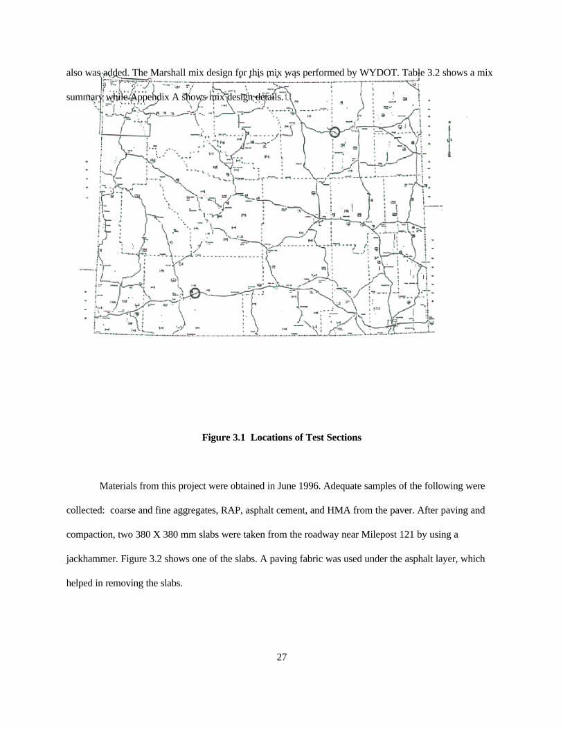
After identifying test sections to be included in the experiment, a testing program was developed,
which included field and laboratory components. The following section describes the components in detail.
To evaluate the characteristics of asphalt mixes in this experiment, two primary laboratory tests
were used. The thermal stress restrained specimen test (TSRST) determined the low-temperature properties
of each mix including temperature and tensile stress at fracture due to thermal cracking. While low
temperature cracking was the main factor in this study, the Georgia loaded wheel tester (GLWT) also was
used to determine the rutting resistance of each mix. The main objective of any pavement engineer is to
obtain a balanced mix that offers good resistance to low temperature cracking and rutting. By performing
the TSRST and GLWT tests, the performance of asphalt mixes at high and low temperatures could be
observed.
Another objective of this study was to evaluate effects of aging on mix performance. Two forms of
aging were used in this experiment. Short-Term Oven Aging (STOA) was performed in accordance to the
standard test method SHRP M-007, Standard Method of Test for Short- and Long-Term Aging of
Bituminous Mixes described in Harrigan, Leahy, and Youtcheff (1994). In this procedure, the asphalt mix
is placed in pans directly after mixing and spread out thinly. The pans are then placed in a 135/C oven for
four hours, after which the mix is compacted. STOA is done to simulate aging that takes place while HMA
is being mixed at the plant and placed in the field. The second type of aging is Long-Term Oven Aging
(LTOA). Samples subjected to LTOA were further aged according to SHRP M-007. In this aging, the
compacted samples are to be placed in an 85/C oven for 120 hours or five days. This is done to simulate
aging that takes place over the service life of the pavement.
Samples tested in the TSRST were obtained from four sources: field slabs, uncompacted mix from
the paver compacted in the lab, unaged mix that was lab mixed and compacted, and STOA mix that was
33
mixed and compacted in the lab. Most lab compacted samples were compacted at the Colorado Department
of Transportation using a linear kneading compactor. Additional samples were compacted at the University
of Wyoming using a press. Compaction details can be found in Chapter 4. By using the samples, the
difference between lab mixes and field mixes could be observed, along with the effects of aging. A
summary presenting the condition of samples tested in the experiment can be found in Table 3.5.
TABLE 3.5 Conditions of Samples Used in Experiment
Sample Mixing Compaction Aging
Field Lab Field LabRolled
LabPress
STOA STOA+LTOA
Field Cores X X
Paver Mix A X X
Paver Mix B X X
Lab Mix A X X
Lab Mix B X X
Lab Mix C X X X
Lab Mix D X X X
Lab Mix E X X X
Lab Mix F X X X
The following mixes were used to make samples for the GLWT: paver mix, unaged lab mix,
STOA lab mix, and STOA + LTOA lab mix. The samples were compacted in the gyratory compactor
according to the compaction method given in SHRP M-002, Standard Method of Test for Preparation of
Compacted Specimens of Modified and Unmodified Hot Mix Asphalt by Means of the SHRP Gyratory
compactor, which is found in Harrigan, Leahy, and Youtcheff (1994). Also, field cores from the project
were obtained from WYDOT and tested in the GLWT. Information from the tests were compared with
results from the TSRST.
34
FIELD DATA
In the spring of 1997, field data were obtained from both test sections. A pavement condition
survey was performed at each site to determine the amount of low-temperature cracking that had occurred
over one winter. This was done by randomly selecting at least eight sites along each project and recording
the amount, type, and severity of cracking in a measured area of pavement. Also, temperature data from
locations near each project were obtained from the Wyoming Water Resource Center located at the
University of Wyoming to determine the temperatures that pavements were subjected to during the winter
months. Equations from the Asphalt Institute were used to determine pavement temperatures. This data
also were compared with findings from laboratory tests to see if the TSRST could be used to predict low-
temperature cracking.
DATA SUMMARY AND EVALUATION
Data such as densities, fracture temperatures, and tensile strengths were recorded from TSRST
testing along with other data described in this chapter. Rut depths were obtained from GLWT testing.
Densities of all samples were evaluated and compared to WYDOT specifications. Statistical analyses were
performed on densities, fracture temperatures, and tensile strengths of TSRST samples. Also, the
correlation of fracture temperatures to rut depths for the various types of samples was explored.
Temperature data were compared to TSRST results and pavement condition surveys to determine if any
correlations were evident. The analysis of data from this study was then used to form conclusions and
recommendations.
35
CHAPTER SUMMARY
This chapter has presented the objectives of this low temperature cracking study and how they
were achieved through laboratory testing and field evaluations. Descriptions of the Point of Rocks and
Kingsbury Road test sections were given, including locations, mix designs, sample collection. Laboratory
tests used in this study and field data collected for analysis were included. How data were used and
analyzed to form conclusions for this study also were presented.
36
37
CHAPTER 4
TESTING AND DATA COLLECTION
INTRODUCTION
Laboratory and field evaluations were performed in this study to observe low temperature cracking
characteristics of asphalt mixes. The focus of laboratory testing was on the thermal stress restrained
specimen test, which concentrates on temperatures and stresses in asphalt mixes when low temperature
thermal cracking occurs. The Georgia loaded wheel tester also was used to examine high temperature
characteristics of rutting in pavements. Background, procedures, and results of the tests are presented in
this chapter.
Field evaluations were performed on the test section sites so that lab and field performance could
be compared. Field data collected included pavement distress surveys, pavement condition index
calculations, and field temperature data. Methods of data collection and results are given in this chapter.
THERMAL STRESS RESTRAINED SPECIMEN TEST
Thermal cracking due to low temperatures is a problem in many parts of the world. Researchers
have been studying thermal cracking for years, and have tried various methods to evaluate low temperature
behavior of asphalt mixes. Data from the evaluations have been used in thermal cracking models developed
to predict low-temperature cracking, such as COLD [Finn et al., 1986], University of Florida model [Ruth
et al., 1982], Texas A&M model [Lytton et al., 1983], and University of Texas model [Shahin and
McCullough, 1972]. Some tests used to provide data for the models include indirect tension test, direct
tension test, direct tensile creep test, flexural bending test, thermal stress restrained specimen test, and
coefficient of thermal expansion and contraction test. According to Vinson et al. (1990), only the thermal
38
stress restrained specimen test and coefficient of thermal expansion and contraction test simulate actual
field conditions and directly measure stress-temperature relationships.
The thermal stress restrained specimen test (TSRST) was first introduced in the 1960s when
Monismith et al. (1965) stated that thermal cracking could be simulated in a laboratory. A specimen was
attached to a fixed frame to keep the sample length constant during cooling while stress, strength, and
temperature data were recorded. Initially the frame was made of Invar steel to reduce change in length of
the frame as temperature decreased. However, this fixed frame method was not successful as frame
deflections during loading would keep the sample from failing [Kanerva, Vinson, and Zeng, 1994]. To
overcome this, Arand (1987) built a displacement feedback loop into the system to constantly correct
specimen length during the test. This prevented stress relaxation in the specimen during the test due to a
flexing frame and allowed sample failure. Further development of the TSRST has been done at Oregon
State University
under SHRP
contract A-003A
and by OEM, Inc.
of Corvallis,
Oregon. A complete
TSRST system is
shown in Figure 4.1.
39
Figure 4.1 Thermal Stress Restrained Specimen Test Apparatus
40
Test Objectives
The objective of the TSRST is to obtain low-temperature characteristics of asphalt concrete mixes,
such as the temperature and stress at which thermal cracking occurs, by subjecting a specimen to an
accelerated test that measures thermal cracking performance. The results enable the asphalt mix designer to
predict how a mix will perform in the field before paving a road, thus eliminating
poor performing pavements that waste valuable tax dollars. Various mixes can be tested in a relatively
short time period and with information from other accelerated performance tests, the most superior mix can
be determined.
The basis of the thermal stress restrained specimen test is to cool an asphalt concrete specimen at a
specified rate, which will cause the specimen to shrink. As shrinking occurs, the specimen is pulled back to
its original length by the device, which builds tensile stress in the asphalt concrete. This continues until the
tensile stress that has accumulated reaches the tensile strength of the sample and specimen breaks.
Test Samples
In this study, both field and lab samples were tested in the TSRST. Field samples were obtained
from slabs taken from the pavements in both test projects. The slabs were cut with a jackhammer in the
field after finishing the lay down operation. Later in the lab, slabs were cored and sawed to obtain samples
suitable for testing in the TSRST machine. All samples were approximately 23 centimeters long. In
addition to the field samples, some samples were compacted in the lab. Initially, a press at the University of
Wyoming was used to compact a few 100 X 100 X 360 mm beams. These beams later were cored to obtain
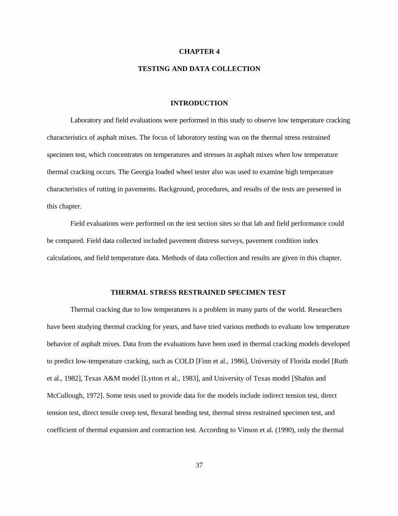
TSRST samples. All additional specimens were compacted by the Colorado Department of Transportation
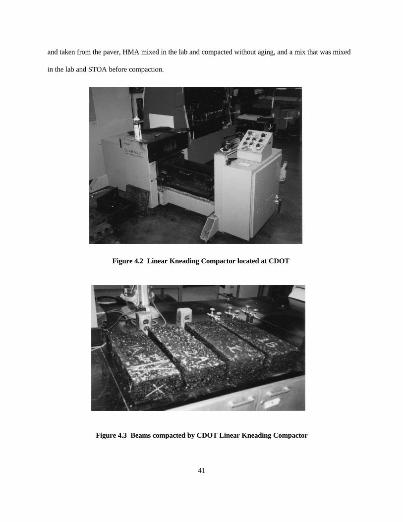
(CDOT) in Denver by means of the linear kneading compactor shown in Figure 4.2. The slabs compacted
at CDOT were 500 X 180 X 100 mm and are shown in Figure 4.3. Three types of mixes were prepared
and tested from each project, with two samples for each type. These mixes were: mix made at the job site
41
and taken from the paver, HMA mixed in the lab and compacted without aging, and a mix that was mixed
in the lab and STOA before compaction.
Figure 4.2 Linear Kneading Compactor located at CDOT
Figure 4.3 Beams compacted by CDOT Linear Kneading Compactor
42
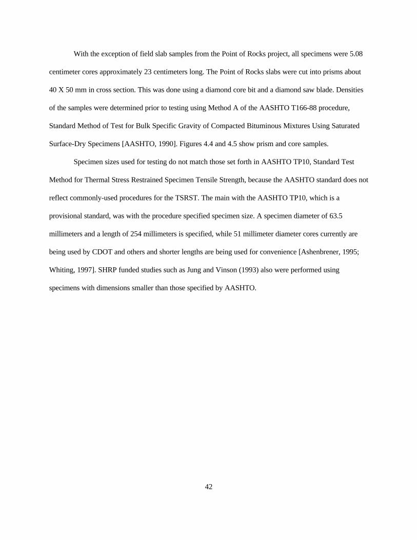
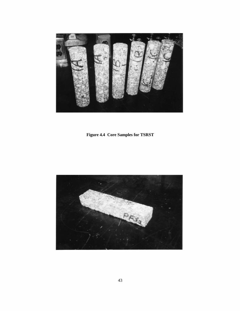
With the exception of field slab samples from the Point of Rocks project, all specimens were 5.08
centimeter cores approximately 23 centimeters long. The Point of Rocks slabs were cut into prisms about
40 X 50 mm in cross section. This was done using a diamond core bit and a diamond saw blade. Densities
of the samples were determined prior to testing using Method A of the AASHTO T166-88 procedure,
Standard Method of Test for Bulk Specific Gravity of Compacted Bituminous Mixtures Using Saturated
Surface-Dry Specimens [AASHTO, 1990]. Figures 4.4 and 4.5 show prism and core samples.
Specimen sizes used for testing do not match those set forth in AASHTO TP10, Standard Test
Method for Thermal Stress Restrained Specimen Tensile Strength, because the AASHTO standard does not
reflect commonly-used procedures for the TSRST. The main with the AASHTO TP10, which is a
provisional standard, was with the procedure specified specimen size. A specimen diameter of 63.5
millimeters and a length of 254 millimeters is specified, while 51 millimeter diameter cores currently are
being used by CDOT and others and shorter lengths are being used for convenience [Ashenbrener, 1995;
Whiting, 1997]. SHRP funded studies such as Jung and Vinson (1993) also were performed using
specimens with dimensions smaller than those specified by AASHTO.
43
Figure 4.4 Core Samples for TSRST
44
Figure 4.5 Prism Sample for TSRST
TSRST Test Procedures
Test procedures for the thermal stress restrained specimen test (TSRST) consisted of two parts:
specimen set up and testing. Procedures suggested by OEM, Inc. were the basis for testing along with
AASHTO TP10. Samples were attached to two aluminum platens using a two-part epoxy, Devcon steel
filled putty and hardener. This was done in an alignment stand that would keep specimen and platens in
proper alignment as shown in Figure 4.6. Poor alignment could result in bending stresses in the sample,
which could alter results [Jung and Vinson, 1994b]. Nine parts putty to one part hardener was used to
create the epoxy as according to
manufacturers directions. Sample
alignment was measured using a small
steel ruler and adjustments were made
accordingly. Holes in the top and bottom
platens were aligned with rods. The epoxy
was allowed to cure overnight.
45
Figure 4.6 TSRST Specimen in Alignment Stand
After curing, the specimen and platens were precooled in an environmental chamber. Precooling
brings the sample temperature to between 2/C and 4/C and takes 30 to 90 minutes [OEM, 1995]. The
environmental chamber was used for precooling to save time by reducing precooling time needed in the
TSRST machine. This procedure allowed more specimens to be tested per bottle of liquid nitrogen and for
precooling of a sample while testing another.
Spring-loaded alignment rods were installed on the assembly, leaving a 2.5 mm gap when the
spring was compressed. Invar rods and LVDT holders were attached and aligned, and ball swivel
connectors were screwed into each end of the assembly. This assembly was then hung in the environmental
cabinet of the TSRST by using the top clevis, and position of the specimen was adjusted with the hand
crank so that the bottom clevis could be connected. A gap was left in the bottom clevis so that no tension
was applied to the sample before testing began. Next, four platinum RTDs were attached to the specimen
using clay. An RTD was placed on each side of the sample, and they were spaced from top to bottom.
LVDTs were placed in their holders and adjusted to give a reading near 0.000 mm, and a temperature
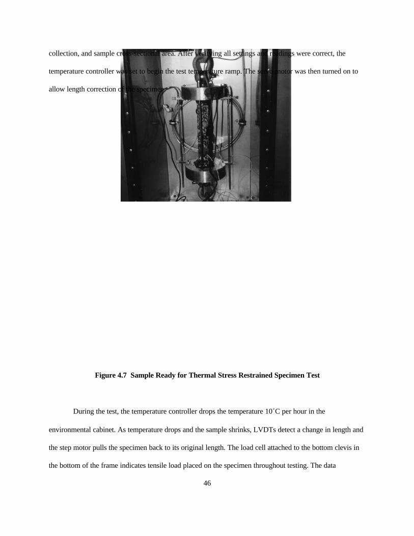
control RTD was hung from the assembly so it was suspended from the top platen. As shown in Figure
4.7, the setup was now ready for precooling.
After setting the temperature controller according to manufacturers directions, liquid nitrogen was
turned on. Specimens were precooled until all four RTDs on the sample had readings between 2 and 4/C.
Data were then entered into the TSRST computer program, such as filename, time interval for data
46
collection, and sample cross-sectional area. After verifying all settings and readings were correct, the
temperature controller was set to begin the test temperature ramp. The servo motor was then turned on to
allow length correction of the specimen.
Figure 4.7 Sample Ready for Thermal Stress Restrained Specimen Test
During the test, the temperature controller drops the temperature 10/C per hour in the
environmental cabinet. As temperature drops and the sample shrinks, LVDTs detect a change in length and
the step motor pulls the specimen back to its original length. The load cell attached to the bottom clevis in
the bottom of the frame indicates tensile load placed on the specimen throughout testing. The data
47
acquisition system scans and records the load, temperatures of the four RTDs, LVDT readings, and test
time at specified intervals throughout the test. One-minute intervals were initially used, but the interval was
increased to two minutes to reduce the large amount of data recorded. Testing would continue until sample
failure, which generally took three or four hours.
According to AASHTO TP10, recorded items include average temperature at failure, load at
failure, δS/δT, which is the slope of the tensile stress vs. temperature curve, and time to failure. Ultimate
strength of the specimen can be determined from the load at failure and the cross-sectional area.
Description of the failure, such as location, shape, and amount of aggregate breakage, were also recorded.
Test Results
The thermal stress restrained specimen test was performed on 23 samples. Eight of the samples
were from the I-90 Kingsbury Road project; the other 15 samples were from the I-80 Point of Rocks
project. More samples were tested from the I-80 project to determine effectiveness of variable methods for
sample preparations. Sample test results are shown in Appendix B and summaries of TSRST test results
are shown in Appendix C.
TSRST results from the Kingsbury Road project are shown in Table 4.1. This table summarizes
densities of field slab and paver mix samples along with fracture temperatures and tensile strengths.
Densities for lab-mixed samples are slightly lower than field samples, with STOA being the lowest.
Fracture temperatures of field compacted samples were slightly lower than the lab compacted samples.
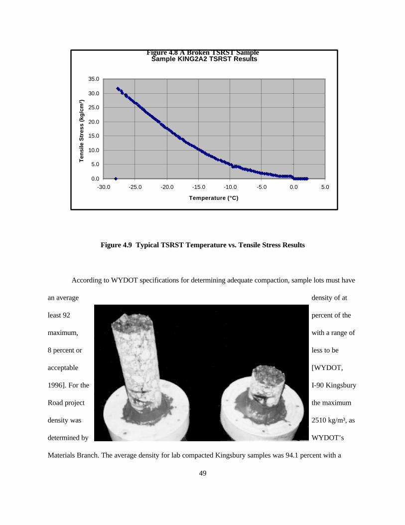
Tensile strengths had some variations. A broken TSRST sample is shown in Figure 4.8, and a typical
graph of temperature versus tensile stress during the test is shown in Figure 4.9.
TABLE 4.1 I-90 Kingsbury Road TSRST Results
48
Sample Condition Density(kg/m³)
TensileStrength(kg/cm²)
FractureTemperature
(/C)
SlopedS/dT(kg/m²//C)
LabCompacted
Paver Mix1 2406 22.5 -25.8 133358
2 2412 31.7 -27.8 17999
Unaged LabMix
1 --- 17.4 -26.0 11390
2 2364 25.4 -24.5 15538
STOA LabMix
1 2308 21.7 -26.9 11249
2 2318 21.9 -23.7 13499
FieldCompacted Field Slab
1 2414 29.2 -28.0 14272
2 2414 26.4 -29.3 16663
49
Sample KING2A2 TSRST Results
0.0
5.0
10.0
15.0
20.0
25.0
30.0
35.0
-30.0 -25.0 -20.0 -15.0 -10.0 -5.0 0.0 5.0
Temperature (°C)
Ten
sile
Str
ess
(kg
/cm
²)
Figure 4.8 A Broken TSRST Sample
Figure 4.9 Typical TSRST Temperature vs. Tensile Stress Results
According to WYDOT specifications for determining adequate compaction, sample lots must have
an average density of at
least 92 percent of the
maximum, with a range of
8 percent or less to be
acceptable [WYDOT,
1996]. For the I-90 Kingsbury
Road project the maximum
density was 2510 kg/m³, as
determined by WYDOT’s
Materials Branch. The average density for lab compacted Kingsbury samples was 94.1 percent with a
50
range of 4.1 percent, acceptable valuesunder WYDOT specifications. The pay factor for such densities is
0.888, which would be a pay deduction if a contractor had these densities in the field. The average density
of the two field samples was 96.2 percent, which is good.
TSRST results for the Point of Rocks samples are shown in Table 4.2. The highest densities and
tensile strengths and lowest fracture temperatures were observed in samples made from field slabs,
followed by samples from ready mix, unaged lab mix, and STOA lab mix. Tests on two STOA lab mix
samples were voided due to malfunctions with the TSRST step motor. In the tests, corrections were not
made for the length of the shrinking sample for an extended period of time. The step motor suddenly tried to
correct for different length by stretching the sample rapidly. Within minutes the sample failed under the
increasing load.
Three samples tested in the TSRST were compacted at UW using a 45,000 kg press. This was
done by placing mix in a 100 X 100 X 360 mm steel mold with a steel spacer on top of the mix. A Tinius-
Olsen press was used to compact the mix by loading the spacer to 36,300 kg and releasing the load twice,
then loading to 36,300 kg and holding at that load for five minutes. The compacted asphalt beam was then
cored to obtain a five centimeter diameter core sample. Results from these samples also are given in Table
4.2.
51
TABLE 4.2 I-80 Point of Rocks TSRST Results
Sample Density(kg/m³)
TensileStrength(kg/m²)
FractureTemperature
(/C)
SlopedS/dT(kg/m²//C)
LabCompacted
LinearKneading
Compactor
Paver Mix1 2284 28.7 -25.2 17858
2 2287 31.3 -26.8 17577
Unaged Lab Mix1 2286 27.3 -24.9 16874
2 2252 23.9 -24.3 15397
STOA Lab Mix
1 2204 --- -24.2 ---
2 2206 16.9 -21.4 10476
3 2179 --- -25.0 ---
4 2188 17.8 -25.8 7312
FieldCompacted Field Slab
1 2318 35.7 -27.6 23904
2 2281 31.3 -27.4 19616
3 2302 34.2 -27.2 26014
4 2332 37.0 -28.1 22428
LabCompacted UW Press
Paver Mix 1 2209 19.7 -27.6 7734
Unaged Lab Mix 1 2239 25.4 -23.7 17014
STOA Lab Mix 1 2241 23.2 -25.8 13640
To determine if sample densities were adequate, samples from the I-80 Point of Rocks project were
divided into four groups. The first group, consisting of two samples from paver mix and two from unaged
lab mix, had an average density of 93.1 percent, a range of 1.5 percent, and a corresponding pay factor of
1.00. This pay factor indicates that a contractor would receive full payment for work of this quality. The
second group, which included four short-term aged lab samples, had an average density of 89.7 percent
which is below 92 percent and is not acceptable. This confirms that there were compaction problems with
the aged mixes. The third group, which were field slabs, had an average density of 93.3 percent and a range
52
of 2.1 percent, which gives a pay factor of 1.00. The fourth group, comprised of samples compacted with
the Tinius-Olsen press at UW, had an average density of 91.1 percent, which also is not acceptable. It
appeared that some aggregate breakage may have occurred during compaction of the samples.
GEORGIA LOADED WHEEL TEST
Accelerated tests to evaluate rutting resistance of flexible pavements have been around for many
years and come in all shapes and sizes. Full-scale testing on test roads performed by traffic simulators have
been used to predict rutting, along with portable methods such as the Accelerated Loading Facility (ALF).
The methods involve full-scale pavements and high costs. However, smaller devices that can be used in a
laboratory have been developed in various parts of the world. The French Rutting Tester and the Hamburg
Wheel Tracking Device have been used extensively to determine rutting and stripping characteristics. Other
tests include the Simple Shear Testing Device from the University of California at Berkeley, Environmental
Conditioning System from Oregon State University, and the Rolling Wheel Machine developed by the
Royal Dutch/Shell Group [Miller, 1995].
The Georgia Loaded-Wheel Tester was developed in 1985 by the Georgia Department of
Transportation (GaDOT) and Georgia Tech to evaluate rutting characteristics of Georgia highways. This
device allows small samples to be tested at temperatures similar to those found in the field. Studies have
found that the GLWT can predict the level of rutting resistance in an asphalt cement mix [Lai and Lee
1990; Miller, 1995]. GaDOT has since used the GLWT extensively and now include the test in their mix
design procedure [Miller, 1995].
Test Objectives
The Georgia loaded-wheel tester, shown in Figure 4.10, is an accelerated test used to determine
rutting resistance of asphalt mixes before using the mixes in the field. This allows for experimentation of
53
different mixes in the lab to produce pavements that perform better in the field. Since asphalt binders are
temperature susceptible, their viscosities decrease with an increase in temperature. As a result, rutting
typically occurs when pavement temperatures are elevated, such as during summer months. The GLWT
allows pavement engineers to heat samples during the test to simulate field conditions. The Georgia loaded-
wheel test consists of a weighted wheel running back and forth over a pressurized rubber tube on the
sample, simulating a tire running over pavement. Rut depths are recorded after various numbers of cycles,
which characterizes
the rutting resistance of the
mix.
Figure 4.10 Georgia Loaded Wheel Tester
Test Samples
In the past, asphalt cement beams were used for testing in the GLWT. However, procedures were
developed at the University of Wyoming to use 150 millimeter cores in the test. Cores are easier to handle,
obtain, and compact than beams, and less material would be needed for testing [Miller, 1995]. A Superpave
54
Gyratory Compactor used for Superpave mix design procedures was used to compact cores in the
laboratory. The gyratory compactor manufactured by Troxler and used at the University of Wyoming is
shown in Figure 4.11. When performing a Superpave design, samples are compacted for a design number
of gyrations. Gyratory compactors also have the capability to compact a sample to a given height, which
makes GLWT testing easier since precast concrete spacers used to hold the sample match the height of the
sample itself. Cores taken from the Kingsbury Road and Point of Rocks projects also were tested in the
GLWT. These cores were obtained by WYDOT after pavement construction.
Figure 4.11 Gyratory Compactor used at the University of Wyoming
Additional samples were made from mix taken from the paver during construction and from cores
cut from completed pavements of the I-80 Point of Rocks and I-90 Kingsbury projects. The only difference
between the samples was the method of compaction, so it was expected that results of paver mix and field
core samples would be similar. Likewise, lab mix that had been short-term oven-aged was expected to
55
simulate new pavement. Lab mixes that had not been aged with those that had been STOA and LTOA were
tested to determine effects of aging on GLWT samples.
Test Procedure
Before testing was performed, the GLWT environmental cabinet was preheated with a core to be
tested. The temperature used to simulate field pavement temperatures during testing was 46.1/C. This
temperature was found to be severe enough to predict rutting and is similar to temperatures found in field
pavements [Miller, 1995]. A core was placed in precast concrete spacers, which were tightened into place.
Initial readings using the rut depth measuring device were taken. A rubber hose with air pressure of 689
kPa was placed in brackets that hold the hose stationary above the sample.The wheel assembly, to which
45.4 kg of steel weights are attached, was then lowered onto the hose. A motor moves the wheel assembly
back and forth across the hose on the sample. One cycle consists of a back and forth motion of the wheel.
The GLWT ran for 1,000 cycles, after which rut depths were measured using a rut depth measuring device.
Rut depths were again recorded after 4,000 and 8,000 cycles. If the total rut depth after 8,000 cycles is less
than 7.62 mm, the sample has passed the test.
Test Results
The Georgia loaded wheel test was performed on 11 samples from each project for a total of 22
samples. This included field cores taken from both projects and samples compacted in the UW lab using the
gyratory compactor. All testing took place at the University of Wyoming. Test results are summarized in
Appendix D.
GLWT results for Kingsbury Road samples are given in Table 4.3. All samples tested in the
GLWT had acceptable rut resistance. Among laboratory prepared mixes, those that had been aged had
smaller rut depths than the unaged samples. However, rut depths on lab-prepared mixes did not correspond
56
with paver mix samples or field cores. It was expected that results from the paver mix, lab mix STOA, and
field core samples would all correspond, but this was not the case. The field cores had the greatest rut
depths of all samples.
57
TABLE 4.3 I-90 Kingsbury Road GLWT Results
Sample Average Density(kg/m³)
Average Rut Depth(mm)
Mix from Paver 2462 2.65
Unaged Lab Mix 2425 2.24
STOA Lab Mix 2439 0.81
STOA + LTOA Lab Mix 2444 0.81
Field Cores 2434 4.56
Densities of Kingsbury Road GLWT samples were quite good when compared to WYDOT
standards. The samples were broken into three groups, with the first made up of paver mix and unaged lab
mix samples. In comparison to the maximum density of 2510 kg/m³, which was
determined by the Materials Program at WYDOT, average density of the first group was 97.3 percent with
a range of 2.2 percent. The corresponding pay factor for the densities are 1.10, which means that the
densities achieved in this lot were high and consistent. The second group was made up of aged lab mixes,
with all being short-term oven aged and some also being long-term oven aged. The samples had an average
density of 97.3 percent of maximum with a range of 0.9 percent, which also has a pay factor of 1.10. The
third group consisted of field cores, which had an average density of 97.0 percent with a range of 0.6
percent. Again, the pay factor worked out to be 1.10, which indicates that the contractor was entitled to a
bonus according to the density of the samples. Overall, densities of the samples compacted in the gyratory
compactor were very similar to samples taken from the field.
Rut depths of the Point of Rocks samples do not vary significantly among different sample types
except for field cores as shown in Table 4.4. There also does not appear to be a trend in rut depth
measurements with respect to aging. Rut depth measurements in all samples from the Point of Rocks
project other than field cores were small, which indicates that this particular mix has great rut resistance
58
properties. This was expected since nearly half the traffic on the I-80 Point of Rocks project is truck traffic
and a strong mix was needed by WYDOT to prevent rutting in this section.
TABLE 4.4 I-80 Point of Rocks GLWT Results
Sample Average Density(kg/m³)
Average Rut Depth(mm)
Mix from Paver 2322 1.09
Unaged Lab Mix 2311 1.02
STOA Lab Mix 2316 1.50
STOA + LTOA Lab Mix 2301 1.07
Field Cores *2253 *4.56* Numbers affected by 19 mm wearing surface course
The field cores from the Point of Rocks project included a 19 mm wearing course on the surface.
It appeared that rutting during the Georgia loaded wheel test may have been due to compaction of the
wearing course, which was an open graded mix that does not possess much structural strength.
When looking at the densities of I-80 Point of Rocks samples, three groups were used. The first
group was paver mix samples, which had an average density of 94.8 percent. No pay factor was computed
due to a small group size, but densities were good. The second group was all six lab prepared samples.
They had an average density of 94.3 percent and a range of 1.1 percent, which gives a pay factor of 1.0.
The third group was the field cores, which had an average density of 92.1 percent, a range of 0.9 percent,
and a corresponding pay factor of 0.583. The low densities of the field cores was due to a 19 mm wearing
course, which comprised almost one-third of the core sample. Field slabs collected before the wearing
course was added had excellent densities, indicating that addition of the wearing course was the cause of
lower densities. Overall, the gyratory compactor used at the University of Wyoming created samples with
consistent densities and appeared to do a good job of reproducing densities found in field pavement slabs.
59
FIELD EVALUATION
After obtaining results from thermal stress restrained specimen tests in the lab, comparisons had to
be made with field performance of pavements at both projects. This was done by performing pavement
distress surveys on each project. Methods used in this study for evaluating pavement distress are found in
Distress Identification Manual for the Long-Term Pavement Performance Project [Strategic Highway
Research Program, 1993], which provides methods of pavement distress categorization according to type,
severity, and quantity. Also, the Pavement Condition Index (PCI) for each project was determined using the
U.S. Army’s PAVER procedure [Shahin and Kohn, 1981]. Data from pavement condition surveys were
compared with actual temperature data taken from near the project sites. Temperature data were obtained
from the Wyoming Water Resource Center located at the University of Wyoming.
In this study, pavement distress surveys focused on transverse cracking of pavements from the I-80
Point of Rocks and I-90 Kingsbury Road projects. Generally, transverse cracks are a result of thermal
cracking due to low temperatures. Since pavements in this study were less than one-year-old when
surveyed, other distresses, such as rutting or fatigue cracking, were not present. Crack severity was
classified as low, moderate, or high. Low severity cracks have a mean width less than 6.4 mm. Moderate
severity cracks have widths between 6.4 and 19 mm, while high severity cracks are wider than 19 mm.
Since performing a distress survey over an entire project would be time consuming, only samples
of each project were surveyed. According to PAVER procedures from Shahin and Kohn (1981), a
minimum of five samples should be surveyed, with more samples being included as pavement condition
variations increase. It was determined that at least eight samples from each project should be surveyed, as
there was not much variation expected in the condition of the new pavements. Data from the random
samples taken throughout the project were then used to calculate the PCI for each pavement. The PCI for a
pavement can range from 0 to 100, with the rating decreasing as a pavement deteriorates.
60
Each sample consisted of two 3.6 m lanes, 0.6 m of inside shoulder, 1.8 m of outside shoulder, at a
length of 30.5 m along the roadway. This provided a sample area of 297 m2, which is within the PAVER
guidelines of 232±93 m2 . Sample locations were chosen by dividing project length into even pieces and
systematically picking samples spaced evenly throughout the project. This would ensure unbiased sample
selection that would not be affected by field conditions.
The Point of Rocks project is about 16 kilometers long, so one sample per 1,600 meters was
surveyed. The first sample location began approximately 800 meters from the west end of the project, as
measured by a car odometer. Each consecutive sample was then located an additional 1,600 meters east,
for a total of nine samples. Two sample locations were changed due to guardrail along the highway, which
did not allow a place for a vehicle to be safely pulled off the roadway. The sample sites were moved to the
nearest safe location. Samples were marked off using a hand odometer, and pavements were surveyed
visually and data recorded. Location, length, and severity of each crack was recorded on data sheets for
nine sample areas.
With the Kingsbury Road project length of eight kilometers, samples had to be spaced
approximately 800 meters apart. The same procedure used for the Point of Rocks survey was used here,
except that samples were spaced at 800 meter intervals throughout the project. Surveys were performed on
westbound lanes only, as eastbound lanes had not yet been constructed. Eleven samples were observed on
the project. An example of low temperature cracking from the Kingsbury test section is shown in Figure
4.12.
61
Figure 4.12 Low Temperature Cracking at Kingsbury Road Test Section
Results of the pavement condition surveys are presented in Appendix E. A summary of the results
is given in Table 4.5. It was apparent that only minimal thermal cracking had occurred over the winter and
spacings between cracks were large. For example, cracks in the Kingsbury Road project appeared to be
spaced about 75 meters apart, meaning that most 30.5 meter long survey samples would not include
cracking. Cracks that did appear on this project were completely across the road. Cracks in the Point of
Rocks project occurred more frequently, but generally were short in length. No cracks completely
traversing the road were observed in Point of Rocks samples. It also was noted that for both projects, all
cracks observed were of low severity — no medium or high severity cracks existed in any survey samples.
As a result of relatively small quantities of cracks with minimal severity, PCIs of these pavements were
quite high, which would be expected from a new pavement.
62
TABLE 4.5 Pavement Condition Survey Results
Point of Rocks Project Kingsbury Road Project
Number of Samples 9 11
Number of Cracks 27 4
Total Crack Length (m) 68 36
Pavement Condition Index 98.7 99.4
Condition Rating Excellent Excellent
TEMPERATURE DATA
Temperature data were collected for sites located as close as possible to each project. Data from
station 487845 located at the Rock Springs Airport were used for the Point of Rocks project, while data
from station 483855 located 14 kilometers east-southeast of Gillette were used for the Kingsbury Road
project. While locations of the stations were approximately 30 to 50 kilometers from the project sites, it
must be understood that Wyoming is a rural state and these stations are the closest available that provide
reliable data on a daily basis. Daily maximum and minimum temperatures covering August 1996 to April
1997 were collected to ensure that the lowest temperatures were included. Some observations of the
temperature data are shown in Table 4.6 while complete data for the 1996-97 winter can be found in
Appendix F.
Pavement temperatures and air temperatures are generally different but related. Asphalt Institute
SP-1 (1995) contains the following equation, which calculates minimum pavement design temperature as a
function of the low air temperature:
Tmin = 0.859 Tair + 1.7/
where Tmin = minimum pavement design temperature in /CTair = minimum air temperature in average year in /C.
63
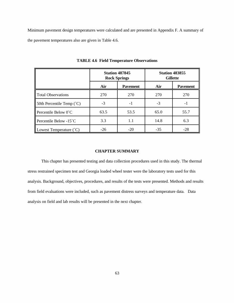
Minimum pavement design temperatures were calculated and are presented in Appendix F. A summary of
the pavement temperatures also are given in Table 4.6.
TABLE 4.6 Field Temperature Observations
Station 487845Rock Springs
Station 483855Gillette
Air Pavement Air Pavement
Total Observations 270 270 270 270
50th Percentile Temp (/C) -3 -1 -3 -1
Percentile Below 0/C 63.5 53.5 65.0 55.7
Percentile Below -15/C 3.3 1.1 14.8 6.3
Lowest Temperature (/C) -26 -20 -35 -28
CHAPTER SUMMARY
This chapter has presented testing and data collection procedures used in this study. The thermal
stress restrained specimen test and Georgia loaded wheel tester were the laboratory tests used for this
analysis. Background, objectives, procedures, and results of the tests were presented. Methods and results
from field evaluations were included, such as pavement distress surveys and temperature data. Data
analysis on field and lab results will be presented in the next chapter.
64
CHAPTER 5
DATA ANALYSIS
INTRODUCTION
Following data collection as well as the field and laboratory testing described in previous chapters,
results were summarized and evaluated. Statistical analyses using one-way ANOVA and general linear
model methods were performed on data to determine the effect of sample preparation on the TSRST
results. This chapter summarizes all the statistical findings in addition to comparisons performed on field
and laboratory data.
STATISTICAL ANALYSIS
A statistical analysis was performed on laboratory test data obtained in this study. One-way
analysis of variance (ANOVA) was performed separately on TSRST and GLWT data for both Point of
Rocks and Kingsbury samples. The analysis of variance method looks at the variance of a regression
analysis and partitions the error into as attributed to the regression and error terms. ANOVA procedures
allow easy calculation of an F statistic which is used to decide if a response is significant [Netter, Kutner,
Nachtsheim, and Wasserman, 1996]. This study utilized the ANOVA method of regression analysis to
determine if sample type, such as field slab, paver mix, unaged lab mix, or STOA lab mix, made a
difference in density, fracture temperature, tensile strength, or rut depth. A simple regression analysis was
conducted to determine the relationship between density and fracture temperature for TSRST samples. In
addition, general linear models were used to determine if sample project had effects on density, fracture
temperature, tensile strength, or rut depth of samples. Using a general model allows for many types of
regression relationships, such as polynomial regression, transformed variables, qualitative predictor
65
variables, and interaction effects [Netter et al., 1996]. The MINITAB computer package was used for all
statistical calculations.
In an effort to compare low and high temperature properties of asphalt mixes included in this
study, fracture temperatures from the TSRST were compared with rut depths from the GLWT for each
sample type. This was done by simply plotting fracture temperature versus rut depth to see if the results
were correlated. The plotting method used was rather unconventional, but this was necessary since rut
depths and fracture temperatures came from completely different samples and could not be compared with
conventional statistical methods.
Analysis on TSRST Data
The focus of laboratory testing for this study was on the thermal stress restrained specimen test
(TSRST). As a result, most of the data analysis focused on results from this test. Statistical results are
summarized in Tables 5.1 and 5.2, while complete statistical results can be found in Appendix G.
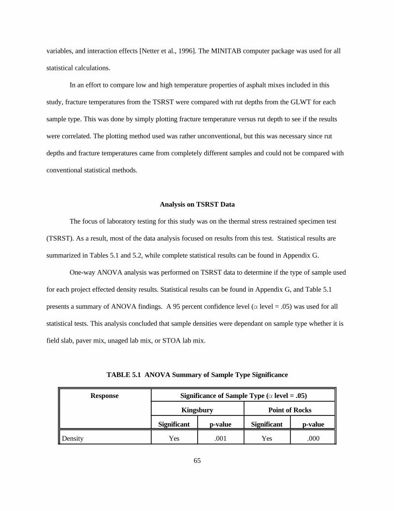
One-way ANOVA analysis was performed on TSRST data to determine if the type of sample used
for each project effected density results. Statistical results can be found in Appendix G, and Table 5.1
presents a summary of ANOVA findings. A 95 percent confidence level (" level = .05) was used for all
statistical tests. This analysis concluded that sample densities were dependant on sample type whether it is
field slab, paver mix, unaged lab mix, or STOA lab mix.
TABLE 5.1 ANOVA Summary of Sample Type Significance
Response Significance of Sample Type (" level = .05)
Kingsbury Point of Rocks
Significant p-value Significant p-value
Density Yes .001 Yes .000
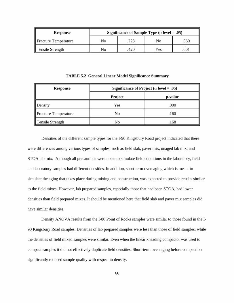
Response Significance of Sample Type (" level = .05)
66
Fracture Temperature No .223 No .060
Tensile Strength No .420 Yes .001
TABLE 5.2 General Linear Model Significance Summary
Response Significance of Project (" level = .05)
Project p-value
Density Yes .000
Fracture Temperature No .160
Tensile Strength No .168
Densities of the different sample types for the I-90 Kingsbury Road project indicated that there
were differences among various types of samples, such as field slab, paver mix, unaged lab mix, and
STOA lab mix. Although all precautions were taken to simulate field conditions in the laboratory, field
and laboratory samples had different densities. In addition, short-term oven aging which is meant to
simulate the aging that takes place during mixing and construction, was expected to provide results similar
to the field mixes. However, lab prepared samples, especially those that had been STOA, had lower
densities than field prepared mixes. It should be mentioned here that field slab and paver mix samples did
have similar densities.
Density ANOVA results from the I-80 Point of Rocks samples were similar to those found in the I-
90 Kingsbury Road samples. Densities of lab prepared samples were less than those of field samples, while
the densities of field mixed samples were similar. Even when the linear kneading compactor was used to
compact samples it did not effectively duplicate field densities. Short-term oven aging before compaction
significantly reduced sample quality with respect to density.
67
As shown in Table 5.2, the general linear model indicated that densities were different for samples
from each project. This was expected, as each project had a different density according to the job mix
formula.
The density analysis indicated that samples taken from field mixes have better densities than
samples made from lab mixes. Methods used to prepare TSRST samples in the lab could not simulate field
densities. If TSRST samples with field densities are needed, they should come from HMA that has been
mixed in the field. Other methods of laboratory sample preparation and compaction may more closely
approximate field compaction. For example, densities of Georgia loaded wheel test samples prepared in the
gyratory compactor were similar to those of field samples. However, modifications would be necessary to
create TSRST samples in the gyratory compactor as it cannot currently accommodate current TSRST
sample lengths.
As shown in Table 5.1, fracture temperatures for TSRST samples appeared to be similar
regardless of sample type. Although fracture temperatures varied slightly from one sample to another, the
variations statistically were not significant. This indicates that even though sample densities were slightly
different, the fracture temperatures in the TSRST were nearly the same. This conclusion would allow the
preparation of samples in the lab to test mixes before they are made in the field. As shown in Table 5.2,
mixes from the Kingsbury Road and Point of Rocks projects had similar fracture temperatures. This
indicates that both asphalt mixes should have similar resistance to low temperature cracking in the field.
Tensile strengths achieved by samples in the TSRST appeared slightly higher in samples made
from field slabs. However, there were significant amounts of variation in recorded results. This is mainly
due to the method of data collection for the TSRST device. Test data are collected at specified intervals,
such as every two minutes. The last stress recorded before fracture was used as the fracture stress. This
incorporates an error, depending on how much longer the sample took to break. Also, random differences in
mix composition and aggregate position could create weak spots in a sample.
68
When tensile strengths at fracture were analyzed statistically, ANOVA concluded that strength was
not dependent on sample type for the Kingsbury project while strength was dependent on sample type for
the Point of Rocks project. The general linear model as shown in Table 5.2 suggests that there was no
difference in tensile strength between the Point of Rocks and Kingsbury Road projects. This confirms past
studies indicating that fracture strengths were rather difficult to reproduce [Jung and Vinson, 1993].
Aging of asphalt mixes in this study affected results from the TSRST. Unaged lab mixes had
slightly lower fracture temperatures than STOA lab mixes. Although laboratory aging did make a
difference in fracture temperatures, aging did not result in samples with performance similar to field
samples.
A simple regression analysis was conducted to determine a relationship between density and
fracture temperature for TSRST samples. A test to determine if linear relationships were similar for each
individual project indicated that there was no difference between the sites. As a result, the analysis
combined samples from both projects. The resulting regression analysis produced a relationship between
density and fracture temperature that had a p-value of 0.028 and an R2 value of 24 percent, which confirms
that a relationship exists but is not strong.
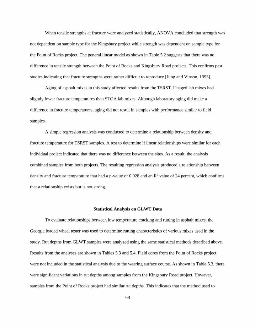
Statistical Analysis on GLWT Data
To evaluate relationships between low temperature cracking and rutting in asphalt mixes, the
Georgia loaded wheel tester was used to determine rutting characteristics of various mixes used in the
study. Rut depths from GLWT samples were analyzed using the same statistical methods described above.
Results from the analyses are shown in Tables 5.3 and 5.4. Field cores from the Point of Rocks project
were not included in the statistical analysis due to the wearing surface course. As shown in Table 5.3, there
were significant variations in rut depths among samples from the Kingsbury Road project. However,
samples from the Point of Rocks project had similar rut depths. This indicates that the method used to
69
make samples for extremely stiff mixes does not significantly affect the GLWT results. However for a
softer mix, mixing and compaction methods can make a difference in GLWT results. For the most reliable
results, field cores should be tested in the GLWT. Overall, no sample from either project failed in the
GLWT, indicating that the mixes had adequate rut resistance.
TABLE 5.3 ANOVA Summary of Sample Type Significance for GLWT Samples
Response Significance of Sample Type (" level = .05)
Kingsbury Point of Rocks
Significant p-value Significant p-value
Rut Depth Yes .000 No .464
TABLE 5.4 General Linear Model Significance Summary for GLWT Samples
Response Significance of Project (" level = .05)
Project p-value
Rut Depth Yes .023
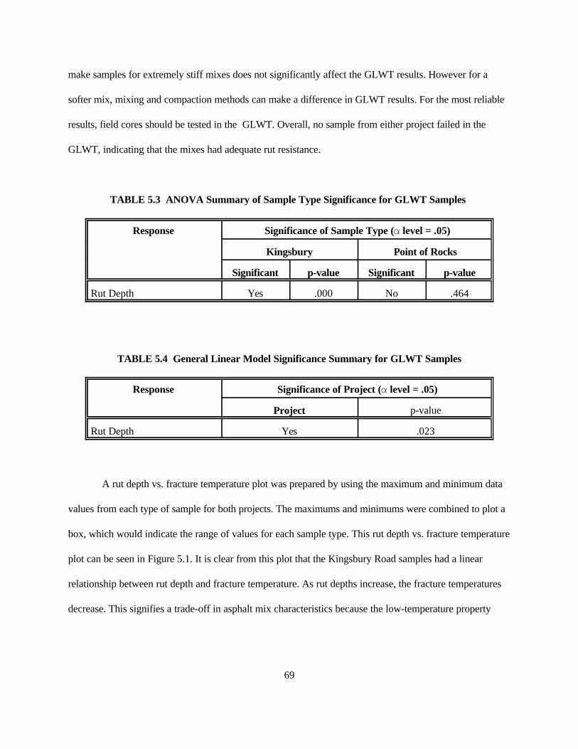
A rut depth vs. fracture temperature plot was prepared by using the maximum and minimum data
values from each type of sample for both projects. The maximums and minimums were combined to plot a
box, which would indicate the range of values for each sample type. This rut depth vs. fracture temperature
plot can be seen in Figure 5.1. It is clear from this plot that the Kingsbury Road samples had a linear
relationship between rut depth and fracture temperature. As rut depths increase, the fracture temperatures
decrease. This signifies a trade-off in asphalt mix characteristics because the low-temperature property
70
Rut Depth vs. Fracture Temperature
-30
-29
-28
-27
-26
-25
-24
-23
-22
-21
-20
0 1 2 3 4 5 6
Rut Depth (mm)
Fra
ctu
re T
emp
erat
ure
(C
)Kingsbury-Paver Mix
Kingsbury-Lab Mix (Unaged)
Kingsbury-Lab Mix (STOA)
Kingsbury-Field Sample
Point of Rocks-Paver Mix
Point of Rocks-Lab Mix(Unaged)
Point of Rocks-Lab Mix(STOA)
Point of Rocks-Field Sample
improves as the high-temperature property deteriorates. However, this relationship is not easily apparent in
the Point of Rocks samples, as their rut depths were similar.
Figure 5.1 Rut Depth vs. Fracture Temperature Plot
ANALYSIS OF FIELD DATA
Field data were collected in the forms of pavement condition surveys and temperature data. As
discussed in previous chapters, pavement condition surveys were used to calculate a pavement condition
index (PCI) for each test section. Both projects had PCI values near 99, which indicates excellent pavement
condition. This was expected as both pavements were less than one-year-old. Distress surveys indicated
that the Point of Rocks section had more total cracking, although no observed cracks completely crossed
the roadway. The Kingsbury section had less total cracking, but virtually every crack observed was
completely across the highway.
71
Pavement distress surveys and pavement condition index (PCI) calculations performed on both I-
80 Point of Rocks and I-90 Kingsbury Road test sections did not show a significant difference in pavement
conditions. Because of the difference in temperatures experienced at both sites, it was not possible to
determine if one field pavement had performed better than the other. Further study of these test sections
after additional service could indicate if this is the case. Also, a test of different mixes used at the same
location could indicate if a ranking of TSRST results would match pavement performance.
As stated previously, temperature data were obtained from sites near both projects. Only daily
minimum temperature data were analyzed for this study. Ranking data from coldest to warmest quickly
showed that Gillette had a significantly higher number of days below -15/C (0/F) than did Rock Springs,
even though the numbers of days below freezing were similar for both sites. It also was apparent that the
minimum recorded temperature for Gillette, -35/C, was quite colder than the -26/C minimum for Rock
Springs.
Point of Rocks Lab and Field Comparisons
Although it is not statistically possible to compare TSRST results with field survey data, general
observations and result comparisons were made. The lowest temperature recorded during the winter of
1996-97 at the Rock Springs airport was -26/C. It was assumed that temperature readings from the
recording station are similar to those experienced at the project. Thermal cracking occurred on the project,
although cracks had not extended across the entire roadway. Most survey samples had cracks present, but
they were generally on the shoulder or across one lane. Temperatures at which Point of Rocks field slab
samples cracked in the TSRST averaged -27.6/C, as seen in Table 4.6. This is just slightly below the
actual low temperature experienced in the field, and well below the lowest pavement temperature. Samples
made from Point of Rocks paver mix broke at an average of -26/C. Lab mixed samples, unaged and short-
72
term aged, broke at slightly warmer temperatures. From TSRST results it would be expected that some
thermal cracking would have occurred, but the amount of cracking would not be extensive since
temperatures did not drop well below the average fracture temperature. This correlates with distress
surveys performed at the project, in which no cracks propagated completely across the pavement.
Kingsbury Road Lab and Field Comparisons
The lowest temperature recorded at the Gillette weather station over the winter of 1996-97 was -
35/C, with four occasions dropping below -30/C. While low temperature crack spacings were quite large,
cracks that had formed were completely across the highway. According to field slabs tested in the TSRST,
the average fracture temperature was -28.7/C. This would indicate that the pavement had been subjected to
critical fracture temperatures on several occasions, and pavement temperatures would have reached this
critical value. Results of distress surveys correspond to TSRST results as the entire roadway width has
cracked.
Point of Rocks vs. Kingsbury Road
A general comparison of the two projects included in this study was made. This would explain
differences in results that were observed due to different materials, environment, and construction. The
Point of Rocks project used a polymer modified AC-20 asphalt and granite aggregate, where the Kingsbury
road project used plain AC-20 asphalt and limestone aggregate. Material use would suggest that Point of
Rocks pavements would be more resistant to low temperature cracking due to stronger asphalt and
aggregate. However, thermal stress restrained specimen tests indicated that statistically both Kingsbury
Road and Point of Rocks projects had similar resistance to thermal cracking. Overall test results indicate
73
that HMA from the Point of Rocks project were generally stiffer than HMA from the Kingsbury Road
project. This is supported by both TSRST and GLWT results.
CHAPTER SUMMARY
Statistical analyses confirmed that TSRST sample densities were dependent upon which project
they came from and how they were made. However, fracture temperatures of the samples were not
statistically dependent on type and were similar regardless of density. Tensile strengths were type
dependent in one asphalt mix and not the other, suggesting that tensile strength may not be a good way of
characterizing low temperature properties. Rut depths were type dependent in the softer Kingsbury Road
mixes, but not in the stiffer Point of Rocks mixes. This indicated that different methods of mixing and
compaction are more significant in softer mixes. Aging did appear to make a difference in test results for
both the TSRST and GLWT, however the aged samples did not simulate field samples as anticipated. A
plot of rut depths from the GLWT vs. fracture temperatures from the TSRST indicated that a linear
relationship is present, with low-temperature properties improving as high-temperature properties
deteriorated.
74
CHAPTER 6
CONCLUSIONS AND RECOMMENDATIONS
INTRODUCTION
This study of low temperature cracking in asphalt mixes was comprised of laboratory and field
components. The thermal stress restrained specimen test (TSRST) and Georgia loaded wheel test (GLWT)
were used in the laboratory to perform testing on asphalt samples from two WYDOT asphalt paving
projects. The TSRST was used to evaluate the effectiveness of testing laboratory and field samples and to
determine if laboratory results compare well with field performance of asphalt pavements. Aging effects on
asphalt mixes also were observed. The GLWT was used to examine the high temperature rutting
characteristics of asphalt mixes. These rutting characteristics were compared with low temperature
characteristics obtained from the TSRST. Field data were recorded by conducting pavement condition
surveys on the test sections and by collecting temperature data near each project. Using all data, the field
performance of asphalt pavements was compared to laboratory test results. Statistical analyses were
performed on laboratory test data to back up observed correlations between sample types, projects, and
results.
CONCLUSIONS
Based on the testing and analysis performed in this study, the following conclusions can be made:
1. The thermal stress restrained specimen test is effective in evaluating low temperature cracking
properties of asphalt mixes. Testing field samples in the device produces results to evaluate
constructed asphalt pavements, while testing laboratory samples produces results to evaluate
asphalt mixes before construction. Results for fracture temperatures were statistically equal
regardless of sample type. Laboratory prepared samples had slightly warmer fracture
75
temperatures, but there was no statistical difference based on sample type even though the samples
had statistically different densities.
2. Current laboratory compaction methods cannot simulate field densities. This is due mixing and
compaction procedures, as field mixed samples compacted in the lab also had densities slightly
below those found in field compacted samples.
3. Tensile strength should not be used to characterize the low temperature cracking resistance of an
asphalt mix. Even though field slab samples had slightly higher tensile strengths than other samples
tested in the TSRST, there were significant variations in strengths recorded in the various tests.
Some of the variations were due to the data collection method, which recorded stress at specified
intervals. Past studies have concluded that tensile stress results were somewhat difficult to
reproduce, which was confirmed in this study.
4. Current asphalt mixes used in Wyoming have adequate rut resistance. The rut depths of the
Kingsbury Road samples had statistically significant variations based on sample type, but were
well within the criteria of the Georgia loaded wheel tester. The Point of Rocks samples had
minimal rutting and rut depths for different sample types were similar. It was apparent that the
Point of Rocks asphalt mix was quite stiff and the Kingsbury Road asphalt mix somewhat softer.
Differences of sample type were more evident in the softer mix.
5. There is a trade-off of high and low temperature performance in asphalt pavement mixes. As low
temperature performance improves, high temperature performance deteriorates. Results from the
TSRST and GLWT were used to make a plot of rut depth vs. fracture temperature, which
indicated that there was a linear relationship between rut depth and fracture temperature among the
various sample types used in this study.
6. Additional field surveys are needed to determine the low temperature performance of the asphalt
mixes observed in this study. Only slight low temperature cracking had occurred at both test
76
sections over their first winter in service. While the Point of Rocks section near Rock Springs had
some cracking, temperatures at the site over the 1996-97 winter did not fall far below fracture
temperatures recorded in TSRST testing. The Kingsbury Road section near Gillette had cracking
completely across the roadway as temperatures at this site dipped well below the fracture
temperatures recorded in TSRST testing on several occasions. These pavements will have
increased thermal cracking after additional years of service if normal temperatures are experienced.
7. The degree of aging of a sample had a significant effect on laboratory test results. However,
laboratory aging did not simulate aging that occurred during mixing and construction of HMA
pavements.
RECOMMENDATIONS
1. While TSRST results were similar for samples tested despite slight density variations, a more
efficient compaction method is needed. Compacting mixes with the linear kneading compactor at
CDOT was time consuming and did not produce samples with densities similar to field samples.
Possibly a method using the gyratory compactor could be developed using a larger sample size.
2. Although field samples can provide the most realistic results in the TSRST, laboratory samples can
provide similar results despite lower densities. Therefore, it is recommended that field samples
should be used when available and laboratory prepared samples should be used to predict
performance prior to construction.
3. The field performance of both I-90 Kingsbury Road and I-80 Point of Rocks projects should be
monitored for additional years of service to determine low temperature characteristics. One winter
is not enough to fully evaluate low temperature cracking resistance. Data collected over a longer
time period will enable field and laboratory results to be fully correlated.
77
4. Further study is necessary to determine if laboratory aging is necessary to simulate aging that
occurs during field mixing and compaction. The method and degree of laboratory aging also should
be investigated.
78
REFERENCES
American Association of State Highway and Transportation Officials. (1990). Standard Specifications for Transportation Materials and Methods of Sampling and Testing. 15th ed. Washington, D.C.: AASHTO.
American Association of State Highway and Transportation Officials. (1993). Standard Test Method for Thermal Stress Restrained Specimen Tensile Strength. AASHTO TP10. 1st ed. Washington,D.C.: AASHTO
American Society for Testing and Materials. (1992). Annual Book of ASTM Standards. Volume 04.03 Road and Paving Materials; Pavement Management Technologies. Philadelphia, PA: ASTM.
Anderson, K.O., B.P. Shields, and J.M. Dacyszyn. (1966). Cracking of Asphalt Pavements Due to Thermal Effects. Proceedings of the Association of Asphalt Paving Technologists.
Anderson, K.O., S.C. Leung, S.C. Poon, and K. Hadipour. (1986). Development of a Method to Evaluate theLowTemperatureTensileProperties ofAsphaltConcrete. Proceedings oftheCanadianTechnicalAsphaltAssociation.
Aschenbrener, Timothy. (1995). Investigation of Low Temperature Thermal Cracking in Hot Mix Asphalt. CDOT-DTD-R-95-7. Denver, CO: Colorado Department of Transportation.
Asphalt Institute. (1995). Superpave Performance Graded Asphalt Binder Specification and Testing (SP-1). Lexington, KY.
Burgess, R.A., O. Kopvillem, and F.D. Young. (1971). Ste. Anne Test Road--Relationships Between Predicted Fracture Temperatures and Low Temperature Field Performance. Proceedings of theAssociation of Asphalt Paving Technologists.
Dempsey, B.J., J. Ingersoll, T.C. Johnson, and M.Y. Shahin. (1980). Asphalt Concrete for Cold Regions. U.S.A. Cold Regions Research and Engineering Laboratory, CRREL Report 80-5.
Finn, F.N., K. Hair, and J. Hilliard. (1976). Minimizing Cracking of Asphalt Concrete Pavements. Proceedings of the Association of Asphalt Paving Technologists.
Fromm, H.J., and W.A. Phang. (1972). A Study of Transverse Cracking in Bituminous Pavements. Proceedings, AAPT, Vol. 41.
Gaw, W.J. (1981). Design Techniques to Minimize Low-Temperature Asphalt Pavement Transverse Cracking. Asphalt Institute. Research Report No. 81-1.
Haas, R.C.G. (1973). A Method of Designing Asphalt Pavements to Minimize Low-Temperature Shrinkage Cracking. Asphalt Institute, Research Report 73-1.
Haas, R., F. Meyer, G. Assaf, and H. Lee. (1987). A Comprehensive Study of Cold Climate Airport Pavement Cracking. Proceedings of the Association of Asphalt Paving Technologists.
Haas, R.C.G. and K.O. Anderson. (1969). A Design Subsystem for the Response of Flexible Pavements at Low Temperatures. Proceedings of the Association of Asphalt Paving Technologists.
Hacker, Diana. (1995). A Writer’s Reference. 3rd ed. Boston, MA: Bedford Books of Martin’s Press.
Harrigan, E.T., R.B. Leahy, and J.S. Youtcheff. (Eds.). (1994). The SUPERPAVE Mix Design System Manual of Specifications, Test Methods, and Practices. Report No. SHRP-A-379. Washington,D.C.: National Research Council.
Hills, J.F., and D. Brien. (1966). The Fracture of Bitumens and Asphalt Mixes by Temperature Induced Stresses. Proceedings of the Association of Asphalt Paving Technologists.
Hindermann, W.L. (1966). Discussion--Symposium on Non-Traffic Load Associated Cracking of Asphalt Pavements. Proceedings of the Association of Asphalt Paving Technologists.
Janoo, V.C., J. Bayer Jr., T.S. Vinson, and R. Haas. (1990). Test Methods to Characterize Low Temperature Cracking. Proceedings of the Fourth Workshop in Paving in Cold Areas, Sapporo,Japan.
Jones, G.M., M.I. Darter, and G. Littlefield. (1968). Design and Evaluation of Asphalt Concrete withRespect to Thermal Cracking. Proceedings of the Association of Asphalt Paving
Technologists.
80
Jung, D.H., and T.S. Vinson. (1994a). Low-Temperature Cracking: Binder Validation. Report No. SHRP-A-399. Washington, D.C.: National Research Council.
Jung, D.H., and T.S. Vinson. (1994b). Low-Temperature Cracking: Test Selection. Report No. SHRP-A-400. Washington, D.C.: National Research Council.
Jung, Duhwoe and T.S. Vinson. (1993). Thermal Stress Restrained Specimen Test To Evaluate Low-Temperature Cracking of Asphalt-Aggregate Mixtures. Transportation Research Record No.1417. Washington, D.C.: National Academy Press.
Kallas, B.F. (1982). Low-Temperature Mechanical Properties of Asphalt Concrete. Asphalt Institute. Research Report No. 82-3.
Kanerva, Hannele K., Ted S. Vinson, and Huayang Zeng. (1994). Low-Temperature Cracking: Field Validation of the Thermal Stress Restrained Specimen Test. Report No. SHRP-A-401. Washington, D.C.: National Research Council.
Kuehl, Robert O. (1994). Statistical Principles of Research Design and Analysis. Belmont, CA: Duxbury Press.
Lai, James S., and Thay-Ming Lee. (1990). Use of a Loaded-Wheel Testing Machine to Evaluate Rutting of Asphalt Mixes. Transportation Research Board 1269.
Littlefield, G. (1967). Thermal Expansion and Contraction Characteristics, Utah Asphaltic Concretes. Proceedings of the Association of Asphalt Paving Technologists.
Martner, Brooks, E. (1986). Wyoming Climate Atlas. Lincoln, NE: University of Nebraska Press.
Miller, Tyler R. (1995). Laboratory Evaluation of Rutting in Asphalt Pavements. Laramie, WY.
Monisimith, C.L., G.A. Secor, and K.E. Secor. (1965). Temperature-Induced Stresses and Deformations in Asphalt Concrete. Proceedings of the Association of Asphalt Paving Technologists.
Netter, John, M.H. Kutner, C.J. Nachtsheim, and W. Wasserman. (1996). Applied Linear Regression Models. 3rd ed. Irwin.
OEM, Inc. (1995). Thermal Stress Restrained Specimen Test User’s Manual. Corvallis, OR.
Owenby, James R., and D.S. Ezell. (1992). Monthly Station Normals of Temperature, Precipitation, and Heating and Cooling Degree Days 1961-90 Wyoming. Climatography of the United States
No. 81. Asheville, N.C.: National Oceanic and Atmospheric Administration (NOAA).
Peurifoy, Robert L., William B. Ledbetter, and Clifford J. Schexnayder. (1996). Construction Planning, Equipment, and Methods. 5th ed. McGraw-Hill.
81
Roberts, Freddy L., Prithvi S. Kankhal, E. Ray Brown, Dah-Yinn Lee, and Thomas W. Kennedy. (1991). Hot Mix Asphalt Materials, Mixture, Design, and Construction. 1st ed. Lanham, MD: NAPA Education foundation.
Ruth, B.E., L.A.K. Bloy, and A.A. Avital. (1982). Prediction of Pavement Cracking at Low Temperatures. Proceedings of the Association of Asphalt Paving Technologists.
Scherocman, James A. (1991). International State-of-the-Art Colloquium on Low-Temperature AsphaltPavement Cracking. Special Report 91-5. United States Army Cold Regions Research and Engineering
Laboratory.
Shahin, M.Y., and B.F. McCullough. (1974). Damage Model for Predicting Temperature Cracking in Flexible Pavements. Transportation Research Record.
Shahin, M.Y., and S.D. Kohn. (1981). Pavement Maintenance Management for Roads and Parking Lots. U.S. Army Construction Engineering Research Laboratory Technical Report M-294. Champaign, IL: United States Army Corps of Engineers.
Strategic Highway Research Program. (1993). Distress Identification Manual for the Long-Term Pavement Performance Project. Report No. SHRP-P-338. Washington, D.C.: National Research Council.
Vinson, T.S., V.C. Janoo, and R.C.G. Haas. (1990). Summary Report on Low Temperature and Thermal Fatigue Cracking. Report No. SHRP-A/IR-90-001. Washington, D.C.: National ResearchCouncil.
82
Wyoming Department of Transportation. (1996). Standard Specifications for Road & Bridge Construction. 1996 ed.
Wyoming Department of Transportation. (1993). Wyoming Vehicle Miles. 1993 ed. WYDOT Transportation Planning Program.
Yoder, E.J., and M.W. Witczak. (1975). Principles of Pavement Design. 2nd ed. New York, NY: John Wiley & Sons.