Page 1 of 45 EVALUATION OF MOTION ESTIMATION TECHNIQUES FOR IMAGES DEGRADED BY ATMOSPHERIC TURBULENCE Michael Vlasov - graduation project Ben-Gurion University of the Negev, Beer-Sheva, Israel Department of Electrical and Computer Engineering Electro-Optical Engineering Unit
Transcript
Page 1 of 45
EVALUATION OF MOTION ESTIMATION TECHNIQUES
FOR IMAGES DEGRADED BY ATMOSPHERIC TURBULENCE
Michael Vlasov - graduation project
Ben-Gurion University of the Negev, Beer-Sheva, IsraelDepartment of Electrical and Computer Engineering
Electro-Optical Engineering Unit
Page 2 of 45
Abstract
Atmospheric turbulence is usually the main limiting factor for long-distance optical
imaging. It distorts the wavefront of the incoming light, which results in image
degradation, mostly by blur and lateral spatio-temporal distortion (image dancing). For
many applications these phenomena are highly undesirable. Distortion, for example,
would affect machine vision applications which require static background scene.
Another example is super-resolution techniques based on frame stacking, which require
registered video stream with sub-pixel relative displacements. Image processing
techniques can be utilized to reduce these effects. Blur can be reduced by methods like
deconvolution. The spatio-temporal movement distortion is usually addressed to using
motion estimation and compensation techniques. The estimation produces a motion
vector field, while the compensation "restores" the distorted image. As a result, a
"boiling" turbulent video can be converted into a "frozen" stream, where turbulent motion
in every frame is compensated relative to a specific time point.
There are a variety of techniques for motion estimation, most common of which are
block matching, and optical flow estimation (as the basic Lucas-Kanade method). This
work focuses on analyzing and evaluating application of these techniques for
compensating local distortions caused by atmospheric turbulence. A variety of statistical
criteria, real life turbulent videos, and turbulence models were used. In order to perform
a numerical evaluation - simplified models were developed for simulating atmospheric
turbulence, which correspond to real life videos. These models feature variable
distortion, blurring and noise. Several hundred motion fields and compensated images
were computed, while specific focus was given to "fine tuning" estimation techniques by
introducing and adjusting various parameters. PSNR and SSIM (structural similarity)
methods were used for motion compensation evaluation. A visual inspection was
performed in order to filter out techniques which produce isolated image artifacts. In
addition, while most of the research in this field focuses on evaluating quality of restored
images, we addressed the fidelity of the estimated motion field itself.
Page 3 of 45
Contents
ABSTRACT..................................................................................................................... 2CONTENTS .................................................................................................................... 3TURBULENCE AND IT’S EFFECT ON IMAGING ...................................................................... 4SIMULATING ATMOSPHERIC TURBULENCE ......................................................................... 5SOLVING THE PROBLEM OF DISPLACEMENTS................................................................... 10MOTION ESTIMATION APPROACH.................................................................................... 11PERFORMANCE EVALUATION MODEL OF MOTION ESTIMATION METHODS ............................ 11MOTION COMPENSATION............................................................................................... 14STATISTICAL COMPARISON ........................................................................................... 15BLOCK MATCHING MOTION ESTIMATION .......................................................................... 17VARIANTS AND RESULTS OF BLOCK MATCHING MOTION ESTIMATION: ................................. 18LUCAS KANADE MOTION ESTIMATION ............................................................................. 31VARIANTS AND RESULTS OF LUCAS KANADE MOTION ESTIMATION:.................................... 32COMPARISON OF LUCAS KANADE AND BLOCK MATCHING MOTION ESTIMATION:................. 42CONCLUSIONS ............................................................................................................. 44REFERENCES .............................................................................................................. 45
Page 4 of 45
Turbulence and it’s effect on imaging
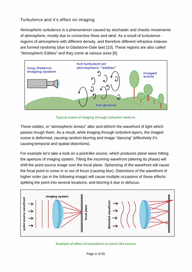
Atmospheric turbulence is a phenomenon caused by stochastic and chaotic movementsof atmosphere, mostly due to convective flows and wind. As a result of turbulence -regions of atmosphere with different density, and therefore different refractive indexesare formed randomly (due to Gladstone-Dale law) [10]. These regions are also called“Atmospheric Eddies” and they come at various sizes [9].
Typical scene of imaging through turbulent medium
These eddies, or “atmospheric lenses” alter and deform the wavefront of light whichpasses trough them. As a result, while imaging through turbulent layers, the imagedscene is deformed, causing random blurring and image “dancing” (effectively it’scausing temporal and spatial distortions).
For example let’s take a look on a point-like source, which produces plane wave hittingthe aperture of imaging system. Tilting the incoming wavefront (altering its phase) willshift the point source image over the focal plane. Spherizing of the wavefront will causethe focal point to come in or out of focus (causing blur). Distortions of the wavefront ofhigher order (as in the following image) will cause multiple occasions of these effects:splitting the point into several locations, and blurring it due to defocus.
Example of effect of turbulence on point-like source
Page 5 of 45
Since these events are highly time dependent – during the integration time (exposure)these effects are accumulated, and additional blurring is introduced. Basically the PSFof a given optical system is no longer limited by diffraction and aberration parameters ofoptics, but also is subject to effects of turbulence.
Turbulence depends on many factors such as temperature, altitude and air pressure,landscape and obstacles, winds, humidity, etc. For example – turbulence is especiallystrong during the day, at low altitudes (due to convective currents caused by hotground). In addition - effect of turbulence on imaged scene also depends on imagingparameters such as: distance, focal length and aperture, integration time, intervalsbetween exposures, integration time, wavelength, etc.
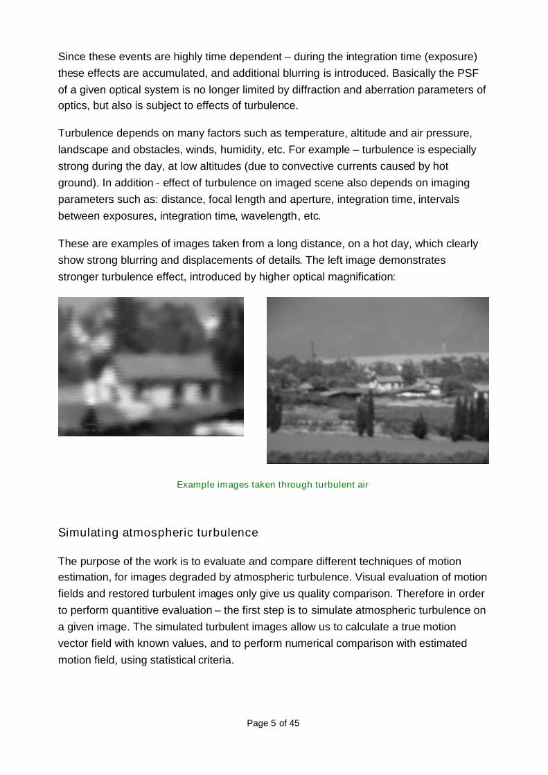
These are examples of images taken from a long distance, on a hot day, which clearlyshow strong blurring and displacements of details. The left image demonstratesstronger turbulence effect, introduced by higher optical magnification:
Example images taken through turbulent air
Simulating atmospheric turbulence
The purpose of the work is to evaluate and compare different techniques of motionestimation, for images degraded by atmospheric turbulence. Visual evaluation of motionfields and restored turbulent images only give us quality comparison. Therefore in orderto perform quantitive evaluation – the first step is to simulate atmospheric turbulence ona given image. The simulated turbulent images allow us to calculate a true motionvector field with known values, and to perform numerical comparison with estimatedmotion field, using statistical criteria.
Page 6 of 45
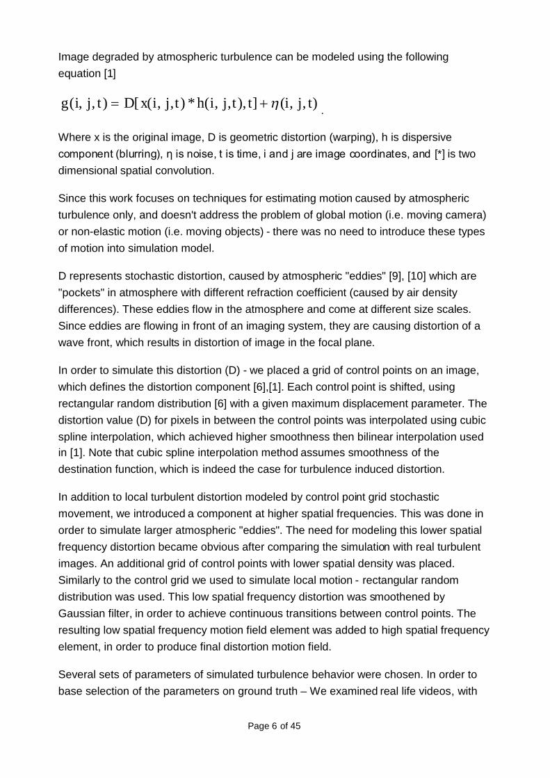
Image degraded by atmospheric turbulence can be modeled using the followingequation [1]
),,(]),,,(*),,([),,( tjittjihtjixDtjig .
Where x is the original image, D is geometric distortion (warping), h is dispersivecomponent (blurring), η is noise, t is time, i and j are image coordinates, and [*] is twodimensional spatial convolution.
Since this work focuses on techniques for estimating motion caused by atmosphericturbulence only, and doesn't address the problem of global motion (i.e. moving camera)or non-elastic motion (i.e. moving objects) - there was no need to introduce these typesof motion into simulation model.
D represents stochastic distortion, caused by atmospheric "eddies" [9], [10] which are"pockets" in atmosphere with different refraction coefficient (caused by air densitydifferences). These eddies flow in the atmosphere and come at different size scales.Since eddies are flowing in front of an imaging system, they are causing distortion of awave front, which results in distortion of image in the focal plane.
In order to simulate this distortion (D) - we placed a grid of control points on an image,which defines the distortion component [6],[1]. Each control point is shifted, usingrectangular random distribution [6] with a given maximum displacement parameter. Thedistortion value (D) for pixels in between the control points was interpolated using cubicspline interpolation, which achieved higher smoothness then bilinear interpolation usedin [1]. Note that cubic spline interpolation method assumes smoothness of thedestination function, which is indeed the case for turbulence induced distortion.
In addition to local turbulent distortion modeled by control point grid stochasticmovement, we introduced a component at higher spatial frequencies. This was done inorder to simulate larger atmospheric "eddies". The need for modeling this lower spatialfrequency distortion became obvious after comparing the simulation with real turbulentimages. An additional grid of control points with lower spatial density was placed.Similarly to the control grid we used to simulate local motion - rectangular randomdistribution was used. This low spatial frequency distortion was smoothened byGaussian filter, in order to achieve continuous transitions between control points. Theresulting low spatial frequency motion field element was added to high spatial frequencyelement, in order to produce final distortion motion field.
Several sets of parameters of simulated turbulence behavior were chosen. In order tobase selection of the parameters on ground truth – We examined real life videos, with
Page 7 of 45
different cases of turbulence. The parameters for each set were selected to make thesimulated results match these real-life videos.
Higher spatial frequency component was chosen by examining consequent frames of aturbulent video. The lower spatial frequency components were chosen after examiningframes with longer interval between them.
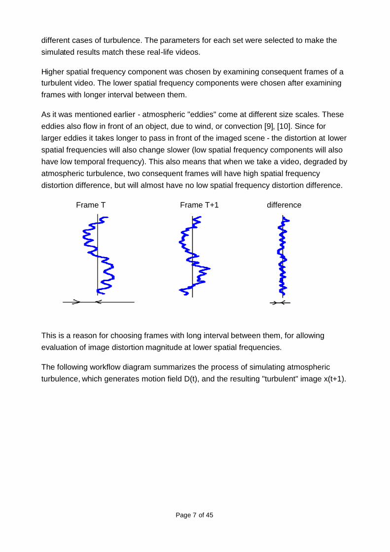
As it was mentioned earlier - atmospheric "eddies" come at different size scales. Theseeddies also flow in front of an object, due to wind, or convection [9], [10]. Since forlarger eddies it takes longer to pass in front of the imaged scene - the distortion at lowerspatial frequencies will also change slower (low spatial frequency components will alsohave low temporal frequency). This also means that when we take a video, degraded byatmospheric turbulence, two consequent frames will have high spatial frequencydistortion difference, but will almost have no low spatial frequency distortion difference.
Frame T Frame T+1 difference
This is a reason for choosing frames with long interval between them, for allowingevaluation of image distortion magnitude at lower spatial frequencies.
The following workflow diagram summarizes the process of simulating atmosphericturbulence, which generates motion field D(t), and the resulting "turbulent" image x(t+1).
Page 8 of 45
distortion parameters (D)
Control points densityMaximum motion amplitudesDistortion spatial frequencies
Random motion fieldgeneration for controlpoints (uniform distribution)
filtering at low spatialfrequency
motion generation at lowspatial frequencies
Blur function (PSF)
Interpolating motionfield for each pixel(cubic spline method)
Atmospheric turbulence model – simulation workflow
Page 9 of 45
Example of true turbulent frames from video "Houses2" (strong turbulence) :
Difference:
Simulated video frames (with parameters which match real turbulence):
Difference:
Page 10 of 45
The following table shows sets of parameters which were input into the simulationmodel, in order to match several real life videos with different degree of turbulence:
Video degree ofturbulence
controlpointsgrid: small
controlpointsgrid: large
high freq.distortionamplitude
low freq.distortionamplitude
low freqdistortionfiltering σ
blurPSF h-size
blurPSF σ-sigma
whitenoisevariance
Fields1 weak 10 80 0.8 1.2 2 2 1 0.0001
Fields2 medium 10 110 1.7 2.9 2 3 2 0.0001
Flir1 very weak 24 144 0.9 1 2 0 0 0.0002
Houses1 strong 10 140 1.9 4 2 3 2 0.00005
Houses2 verystrong 18 144 2.8 6.5 1 4 3 0.0001
Input parameters into atmospheric turbulence simulation model
Solving the problem of displacements
There are two main effects of turbulence: Blurring and spatio-temporal displacements.Blurring causes loss of fine details since the spreading of PSF function causes thehigher spatial frequencies to be attenuated. For long exposures for example (or a resultof frame stacking), the integration of blur and displacement effects can be regarded as aGaussian blur [6]. For short exposure video frames, however, these two phenomenaneed to be treated separately. Blurring is hard to formulize, since it causes by variousfactors such as defocus and higher order PSF distortions, integration of displaced points(with various levels of distortion). There are many methods of reconstruction the blurredimage – for example blind deconvolution, or Kurtosis minimizations. We will not coverthis subject here.
Spatio-temporal displacements cause loss of location and time information for details.This is especially harmful for motion detection algorithms in machine vision, and forcompression difference based algorithms. This work focuses on estimating andrestoring spatial displacements of image at software level, using common motionestimation techniques, and evaluating their performance for this purpose. Apart from thesimulation model – we did not address temporal displacements of image. They areusually less harmful for most popular applications, and reconstructing them wouldrequire implementing three dimensional motion estimation algorithms (2D spatial andtemporal).
Page 11 of 45
Motion estimation approach
Using motion estimation is a practical way to compensate turbulence induceddisplacements, while working on a software level. Most popular methods in this field areeither based on block matching, or on gradient methods (i.e. Lucas Kanade).Implementing motion estimation algorithms on a set of two images degraded byturbulence (reference frame and distorted frame) allow us to build a map of motionvectors, which is called “motion field”. Using this field we can restore the image, and“undo” the effects of turbulent induced displacements.
Motion estimation concept
Since in practice we can not obtain “original” or undistorted image – there is a need toproduce a good reference frame. For example using time-averaged frame, taken over a
specific period of time around the current time period of time: tt 0 .As a compromise,
we can use one of the frames as a reference, at specific time intervals.
Displacements caused by atmospheric turbulence are smooth or “elastic”. We will notaddress here the problem of camera movement (which is usually described by varioustransformation models) and the problem of moving objects. These movements need tobe dealt with separately.
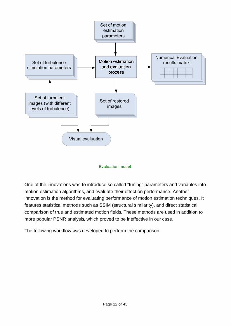
Performance evaluation model of motion estimation methods
In order to evaluate performance of motion estimation methods for the purpose ofcompensating motion and displacements induced by atmospheric turbulence - anevaluation model was built, which included several entities: Set of real life videos withvarying level of atmospheric turbulence, atmospheric turbulence simulation model with aset of parameters, motion estimation algorithms with a set of “tuning” parameters,motion compensation algorithms, and finally the estimation fidelity evaluation algorithm.
Page 12 of 45
Set of turbulentimages (with differentlevels of turbulence)
Set of turbulencesimulation parameters
Numerical Evaluationresults matrix
Set of motionestimationparameters
Set of restoredimages
Visual evaluation
Evaluation model
One of the innovations was to introduce so called “tuning” parameters and variables intomotion estimation algorithms, and evaluate their effect on performance. Anotherinnovation is the method for evaluating performance of motion estimation techniques. Itfeatures statistical methods such as SSIM (structural similarity), and direct statisticalcomparison of true and estimated motion fields. These methods are used in addition tomore popular PSNR analysis, which proved to be ineffective in our case.
The following workflow was developed to perform the comparison.
Page 13 of 45
Workflow of motion estimating process
Workflow of evaluation process
Page 14 of 45
Note that original image is fed twice into turbulence simulation process, in order tosimulate two turbulent images at different time intervals (T1 and T2). Then turbulentimage1 (at T1) is regarded as "reference".
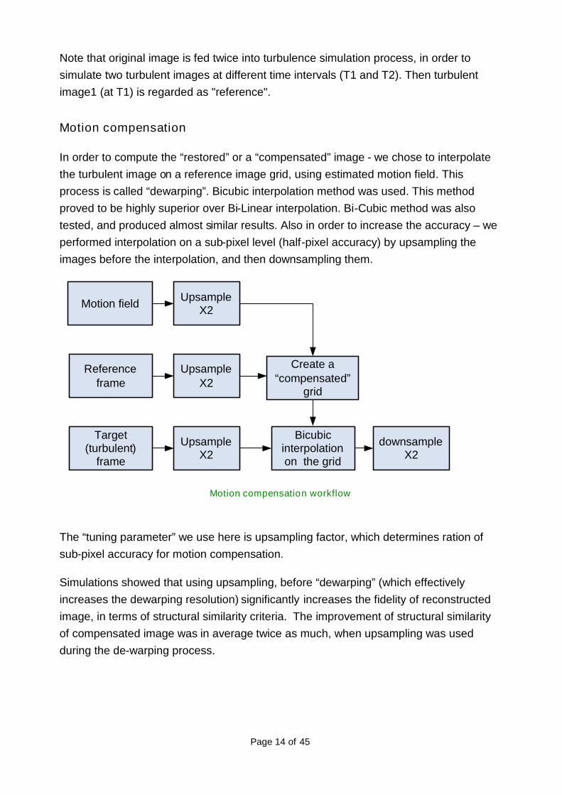
Motion compensation
In order to compute the “restored” or a “compensated” image - we chose to interpolatethe turbulent image on a reference image grid, using estimated motion field. Thisprocess is called “dewarping”. Bicubic interpolation method was used. This methodproved to be highly superior over Bi-Linear interpolation. Bi-Cubic method was alsotested, and produced almost similar results. Also in order to increase the accuracy – weperformed interpolation on a sub-pixel level (half-pixel accuracy) by upsampling theimages before the interpolation, and then downsampling them.
Motion field
Referenceframe
Target(turbulent)
frame
UpsampleX2
UpsampleX2
Create a“compensated”
grid
UpsampleX2
Bicubicinterpolationon the grid
downsampleX2
Motion compensation workflow
The “tuning parameter” we use here is upsampling factor, which determines ration ofsub-pixel accuracy for motion compensation.
Simulations showed that using upsampling, before “dewarping” (which effectivelyincreases the dewarping resolution) significantly increases the fidelity of reconstructedimage, in terms of structural similarity criteria. The improvement of structural similarityof compensated image was in average twice as much, when upsampling was usedduring the de-warping process.
Page 15 of 45
Statistical Comparison
In order to provide reliable comparison and evaluation results – we used severalmethods to compare the results of different motion estimation techniques:
Direct Comparison of motion fields:
Most works in the field of motion estimation evaluate the similarity between thecompensated images, usually by computing PSNR. Since our main purpose was toevaluate motion estimated methods, and not the compensation techniques, weintroduced direct comparison of motion fields, both the magnitude and the direction.
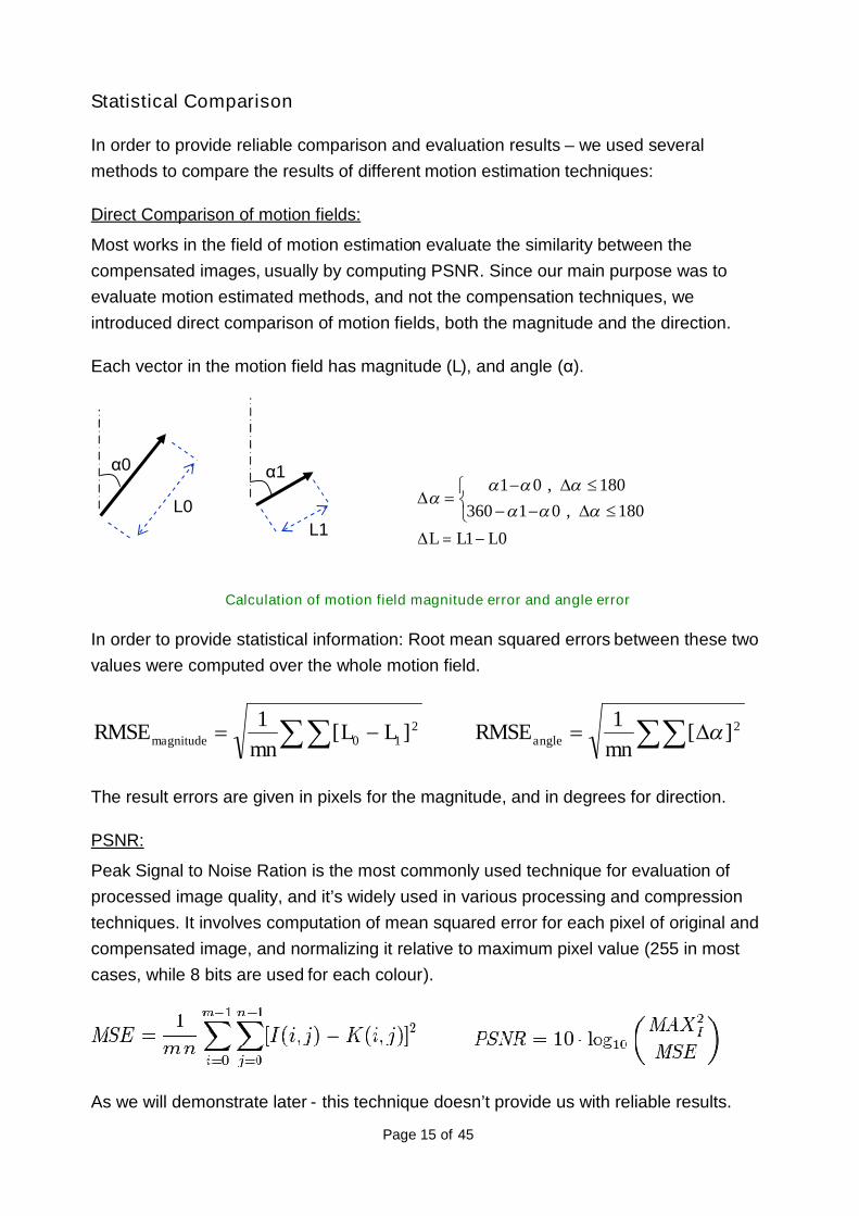
Each vector in the motion field has magnitude (L), and angle (α).
Calculation of motion field magnitude error and angle error
In order to provide statistical information: Root mean squared errors between these twovalues were computed over the whole motion field.
2210 ][1][1
mnRMSELL
mnRMSE anglemagnitude
The result errors are given in pixels for the magnitude, and in degrees for direction.
PSNR:
Peak Signal to Noise Ration is the most commonly used technique for evaluation ofprocessed image quality, and it’s widely used in various processing and compressiontechniques. It involves computation of mean squared error for each pixel of original andcompensated image, and normalizing it relative to maximum pixel value (255 in mostcases, while 8 bits are used for each colour).
As we will demonstrate later - this technique doesn’t provide us with reliable results.
L1L0
α0 α1
01
180,01360180,01
LLL
Page 16 of 45
SSIM:
Structural Similarity Index is a much more reliable technique for comparing the similaritybetween images. While PSNR takes into account only values of a single pixel and sumsit, SSIM technique takes into account surrounding pixel values by calculating statisticalparameters over a certain window. This produces results which are much more similarto visual perception, and much more immune to noise.
SSIM index is calculated over a certain image block:
Whereμx, μy are averages, σx, σy are variances, σxy is covariance. X,Y are two
images under test.
The results are in percents, while 100% represent images with perfect match, and 0%represents images with no match at all.
We computed two SSIM indices: one between original image and the distorted one. Andanother one between original image and one which was motion compensated. Thedifference between these two SSIM indices is called “SSIM improvement”, and it showshow much motion compensation improved the image, which was degraded byturbulence.
PSNR vs. SSIM:
The following is an example which compares SSIM and PSNR for a certain case.
We can clearly see that method 1 (LK) produces much cleaner, and more accurateresult then method 2 (BM). This is also confirmed by analysis and comparison ofestimated and true motion fields (1.88 pixel average error compared to 2.67 pixels)Visual inspection of videos, which were compensated using both methods – alsoshowed clear superiority of method 1 (LK).
The calculated SSIM index improvement for the first method is 9.38%, and for thesecond (the less accurate) method is 7.05%. However the PSNR improvement is theopposite – 0.67dB in first method versus 3.19dB in second one. This clearly does notrepresent the true difference in accuracies of compensated images.
Since similar results were produced over a wide range of simulations – it is clear thatPSNR technique can not be used for our purpose of comparing methods of motionestimation, in case of videos degraded by atmospheric turbulence.
Block matching motion estimation
Block matching is a popular method for motion estimation, which is widely used in videocompression, particularly due to its low computational cost which enables it’s use evenin real time applications.
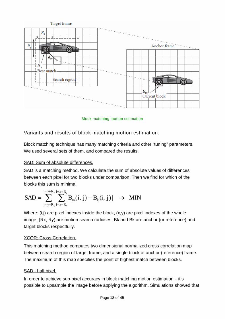
The idea is to divide image into blocks, while for each block we assume constantmotion. First we pick a block in a reference frame (anchor frame), and then in thefollowing frame (target frame) we search, within a certain “search region”, for a blockwhich matches the target block using some kind of comparison criteria. The differencebetween coordinates of block inside the reference frame, and the matching block insidethe target frame, equals to motion vector of this region.
Page 18 of 45
Block matching motion estimation
Variants and results of block matching motion estimation:
Block matching technique has many matching criteria and other “tuning” parameters.We used several sets of them, and compared the results.
SAD: Sum of absolute differences.
SAD is a matching method. We calculate the sum of absolute values of differencesbetween each pixel for two blocks under comparison. Then we find for which of theblocks this sum is minimal.
MIN|),(),(|
y
y
x
x
Ryj
Ryj
Rxi
Rxikm jiBjiBSAD
Where: (i,j) are pixel indexes inside the block, (x,y) are pixel indexes of the wholeimage, (Rx, Ry) are motion search radiuses, Bk and Bk are anchor (or reference) andtarget blocks respectfully.
XCOR: Cross-Correlation.
This matching method computes two-dimensional normalized cross-correlation mapbetween search region of target frame, and a single block of anchor (reference) frame.The maximum of this map specifies the point of highest match between blocks.
SAD - half pixel.
In order to achieve sub-pixel accuracy in block matching motion estimation – it’spossible to upsample the image before applying the algorithm. Simulations showed that
Page 19 of 45
this has little effect on fidelity on motion estimation, and doesn’t justify the method.Videos with high turbulence distortions will have especially low benefit from using sub-pixel motion estimation, since the overall motion magnitude is much larger then a pixel.
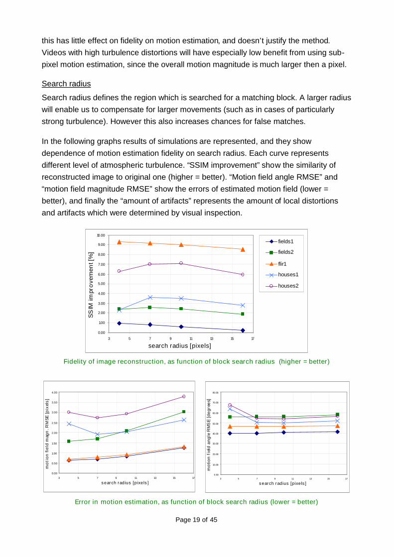
Search radius
Search radius defines the region which is searched for a matching block. A larger radiuswill enable us to compensate for larger movements (such as in cases of particularlystrong turbulence). However this also increases chances for false matches.
In the following graphs results of simulations are represented, and they showdependence of motion estimation fidelity on search radius. Each curve representsdifferent level of atmospheric turbulence. “SSIM improvement” show the similarity ofreconstructed image to original one (higher = better). “Motion field angle RMSE” and“motion field magnitude RMSE” show the errors of estimated motion field (lower =better), and finally the “amount of artifacts” represents the amount of local distortionsand artifacts which were determined by visual inspection.
0.00
1.00
2.00
3.00
4.00
5.00
6.00
7.00
8.00
9.00
10.00
3 5 7 9 11 13 15 17
search radius [pixels]
SS
IMim
pro
vem
ent[
%]
fields1
fields2
flir1
houses1
houses2
Fidelity of image reconstruction, as function of block search radius (higher = better)
Error in motion estimation, as function of block search radius (lower = better)
0.00
0.50
1.00
1.50
2.00
2.50
3.00
3.50
4.00
3 5 7 9 11 13 15 17
search radius [pixels]
mo
tio
nfi
eld
mag
n.R
MS
E[p
ixel
s]
0.00
10.00
20.00
30.00
40.00
50.00
60.00
70.00
80.00
3 5 7 9 11 13 15 17
search radius [pixels]
mo
tio
nfi
eld
an
gle
RM
SE
[de
gre
es]
Page 20 of 45
0
1
1
2
2
3
3
4
3 5 7 9 11 13 15 17
search radius [pixels]
amo
unt
of
arte
fact
s
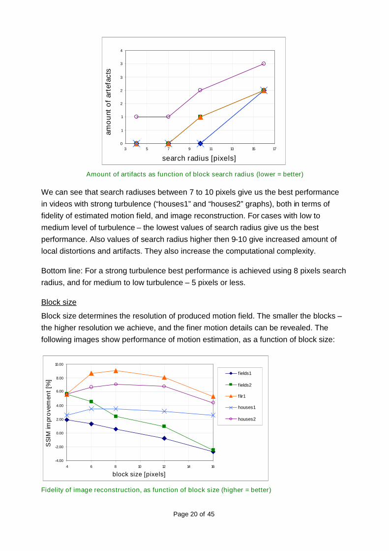
Amount of artifacts as function of block search radius (lower = better)
We can see that search radiuses between 7 to 10 pixels give us the best performancein videos with strong turbulence (“houses1” and “houses2” graphs), both in terms offidelity of estimated motion field, and image reconstruction. For cases with low tomedium level of turbulence – the lowest values of search radius give us the bestperformance. Also values of search radius higher then 9-10 give increased amount oflocal distortions and artifacts. They also increase the computational complexity.
Bottom line: For a strong turbulence best performance is achieved using 8 pixels searchradius, and for medium to low turbulence – 5 pixels or less.
Block size
Block size determines the resolution of produced motion field. The smaller the blocks –the higher resolution we achieve, and the finer motion details can be revealed. Thefollowing images show performance of motion estimation, as a function of block size:
-4.00
-2.00
0.00
2.00
4.00
6.00
8.00
10.00
4 6 8 10 12 14 16
block size [pixels]
SS
IMim
pro
vem
ent
[%]
f ields1
f ields2
f lir1
houses1
houses2
Fidelity of image reconstruction, as function of block size (higher = better)
Page 21 of 45
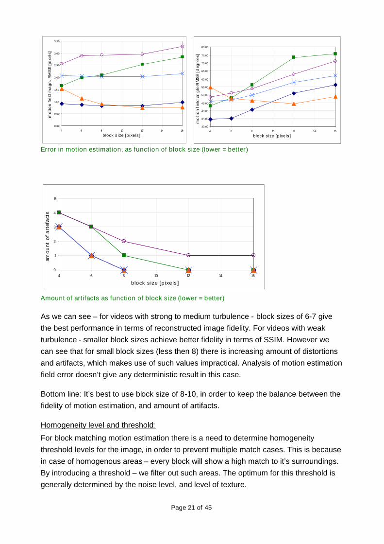
Error in motion estimation, as function of block size (lower = better)
0
1
2
3
4
5
4 6 8 10 12 14 16
block size [pixels]
amo
un
to
fa
rtef
act
s
Amount of artifacts as function of block size (lower = better)
As we can see – for videos with strong to medium turbulence - block sizes of 6-7 givethe best performance in terms of reconstructed image fidelity. For videos with weakturbulence - smaller block sizes achieve better fidelity in terms of SSIM. However wecan see that for small block sizes (less then 8) there is increasing amount of distortionsand artifacts, which makes use of such values impractical. Analysis of motion estimationfield error doesn’t give any deterministic result in this case.
Bottom line: It’s best to use block size of 8-10, in order to keep the balance between thefidelity of motion estimation, and amount of artifacts.
Homogeneity level and threshold:
For block matching motion estimation there is a need to determine homogeneitythreshold levels for the image, in order to prevent multiple match cases. This is becausein case of homogenous areas – every block will show a high match to it’s surroundings.By introducing a threshold – we filter out such areas. The optimum for this threshold isgenerally determined by the noise level, and level of texture.
0.00
0.50
1.00
1.50
2.00
2.50
3.00
3.50
4 6 8 10 12 14 16
block size [pixels]
mo
tio
nfi
eld
ma
gn
.R
MS
E[p
ixel
s]
30.00
35.00
40.00
45.00
50.00
55.00
60.00
65.00
70.00
75.00
80.00
4 6 8 10 12 14 16
block size [pixels]
mo
tio
nfi
eld
ang
leR
MS
E[d
egre
es]
Page 22 of 45
The following method was used for calculating homogeneity: We sort all the pixels froma specific block into a row vector, and calculate difference between highest and thelowest values. Some smoothening filter need to be used prior the calculation, in order toprovide robustness against noise.
Homogeneity threshold determines sensitivity of the algorithm to noise, and itsrobustness. These are results of altering this value, and the effect on motion estimationfidelity:
-2.00
0.00
2.00
4.00
6.00
8.00
10.00
0 5 10 15 20 25 30 35 40
homogenical threshold
SS
IMim
pro
vem
ent
[%]
f ields1
fields2
flir1
houses1
houses2
Fidelity of image reconstruction, as function of homogeneity threshold (higher = better)
Error in motion estimation, as function of homogeneity threshold (lower = better)
0.00
0.50
1.00
1.50
2.00
2.50
3.00
3.50
0 5 10 15 20 25 30 35 40
homogenical threshold
mot
ion
fiel
dm
agn.
RM
SE
[px]
0.00
10.00
20.00
30.00
40.00
50.00
60.00
70.00
80.00
90.00
100.00
0 5 10 15 20 25 30 35 40
homogenical threshold
mo
tion
field
ang
leR
MS
E[d
egre
es]
Page 23 of 45
0
1
1
2
2
3
0 5 10 15 20 25 30 35 40
homogenical threshold
amo
un
to
fa
rtef
act
s
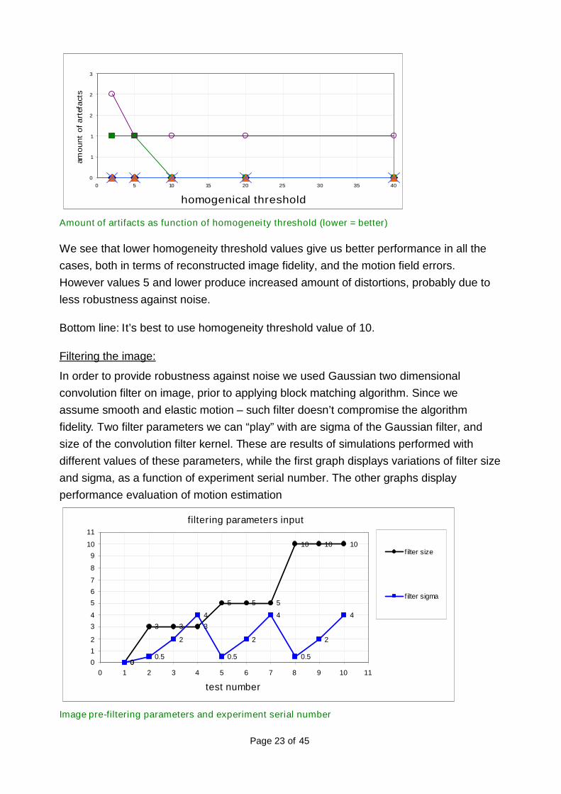
Amount of artifacts as function of homogeneity threshold (lower = better)
We see that lower homogeneity threshold values give us better performance in all thecases, both in terms of reconstructed image fidelity, and the motion field errors.However values 5 and lower produce increased amount of distortions, probably due toless robustness against noise.
Bottom line: It’s best to use homogeneity threshold value of 10.
Filtering the image:
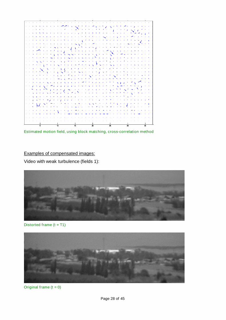
In order to provide robustness against noise we used Gaussian two dimensionalconvolution filter on image, prior to applying block matching algorithm. Since weassume smooth and elastic motion – such filter doesn’t compromise the algorithmfidelity. Two filter parameters we can “play” with are sigma of the Gaussian filter, andsize of the convolution filter kernel. These are results of simulations performed withdifferent values of these parameters, while the first graph displays variations of filter sizeand sigma, as a function of experiment serial number. The other graphs displayperformance evaluation of motion estimation
filtering parameters input
0
3 3 3
5 5 5
10 10 10
00.5
2
4
0.5
2
4
0.5
2
4
0
1
2
3
4
5
6
7
8
9
10
11
0 1 2 3 4 5 6 7 8 9 10 11
test number
f ilter size
filter sigma
Image pre-filtering parameters and experiment serial number
Page 24 of 45
-2.00
0.00
2.00
4.00
6.00
8.00
10.00
0 1 2 3 4 5 6 7 8 9 10 11
test number
SS
IMim
pro
vem
ent
[%]
Fidelity of image reconstruction, as function of filtering parameters (higher = better)
Error in motion estimation, as function of filtering parameters (lower = better)
0
1
1
2
2
3
0 1 2 3 4 5 6 7 8 9 10 11
test number
amo
un
to
far
tefa
cts
Amount of artifacts as function of filtering parameters (lower = better)
It’s clear that test number 6, with filter size = 5 and sigma = 2, produce best overallresults. It’s the only case in which there is a low amount of artifacts and distortions forall the cases of turbulence. In terms of estimated field error – this test, along with testnumber 7 – produce the best overall results. And also in terms of reconstructed image
0.00
1.00
2.00
3.00
4.00
5.00
6.00
0 1 2 3 4 5 6 7 8 9 10 11test number
mo
tio
nfi
eld
ma
gn
.R
MS
E[p
ixel
s]
0.00
10.00
20.00
30.00
40.00
50.00
60.00
70.00
80.00
90.00
100.00
0 1 2 3 4 5 6 7 8 9 10 11
test number
mo
tio
nfi
eld
ang
leR
MS
E[d
eg
rees
]
Page 25 of 45
fidelity – tests number 6 and 7 produce the best result for almost all cases (except“fields2” video test).
Bottom line: It’s best to filter the image before applying the algorithm, and the filteringparameters which produce the best overall results are: sigma = 2 and kernel size = 5.
Examples of motion fields:
The following are examples of applying several different methods of block matchingmotion estimation on image which was distorted by simulated atmospheric turbulence.
Original image
Image influenced by simulated atmospheric turbulence
Page 26 of 45
Actual motion field used for warping the images
Estimated motion field, using block matching, SAD, strong filtering method
Page 27 of 45
Estimated motion field, using block matching, SAD, weak filtering method
Estimated motion field, using block matching, half-pixel SAD, weak filtering method
Page 28 of 45
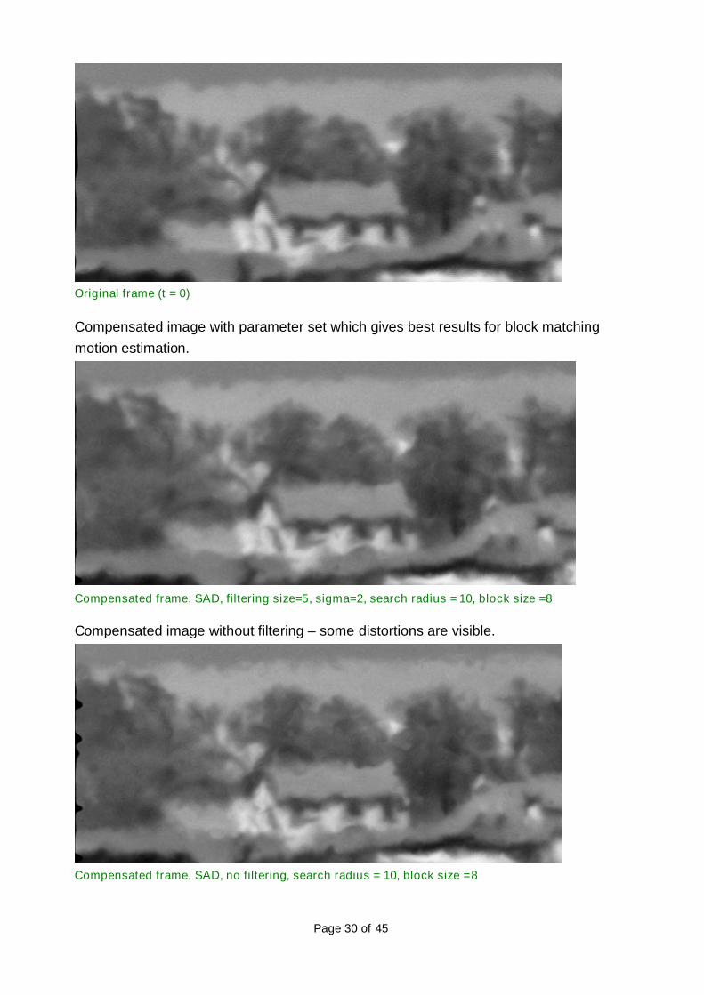
Estimated motion field, using block matching, cross-correlation method
Examples of compensated images:
Video with weak turbulence (fields 1):
Distorted frame (t = T1)
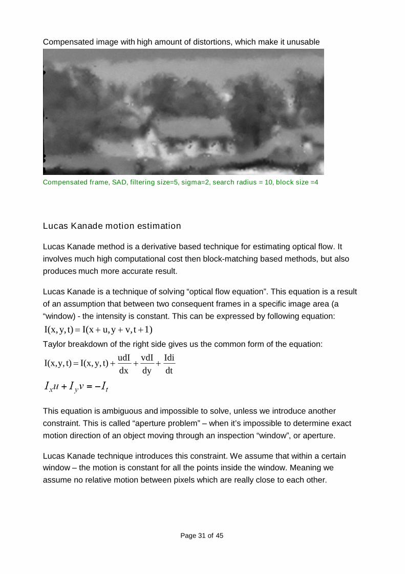
Original frame (t = 0)
Page 29 of 45
Compensated image with parameter set which gives best results for block matchingmotion estimation.
Example of compensated image with high motion estimation fidelity, but which isunusable due to high amount of local distortions and artifacts. In this particular case thedistortions happened due to small block size, and large search radius, which causedhigh amount of false block matching, and as a result - distortions during compensation.
Lucas Kanade method is a derivative based technique for estimating optical flow. Itinvolves much high computational cost then block-matching based methods, but alsoproduces much more accurate result.
Lucas Kanade is a technique of solving “optical flow equation”. This equation is a resultof an assumption that between two consequent frames in a specific image area (a“window) - the intensity is constant. This can be expressed by following equation:
1)tv,yu,I(xt)y,I(x, Taylor breakdown of the right side gives us the common form of the equation:
dtIdi
dyvdI
dxudIt)y,I(x,t)y,I(x,
This equation is ambiguous and impossible to solve, unless we introduce anotherconstraint. This is called “aperture problem” – when it’s impossible to determine exactmotion direction of an object moving through an inspection “window”, or aperture.
Lucas Kanade technique introduces this constraint. We assume that within a certainwindow – the motion is constant for all the points inside the window. Meaning weassume no relative motion between pixels which are really close to each other.
Page 32 of 45
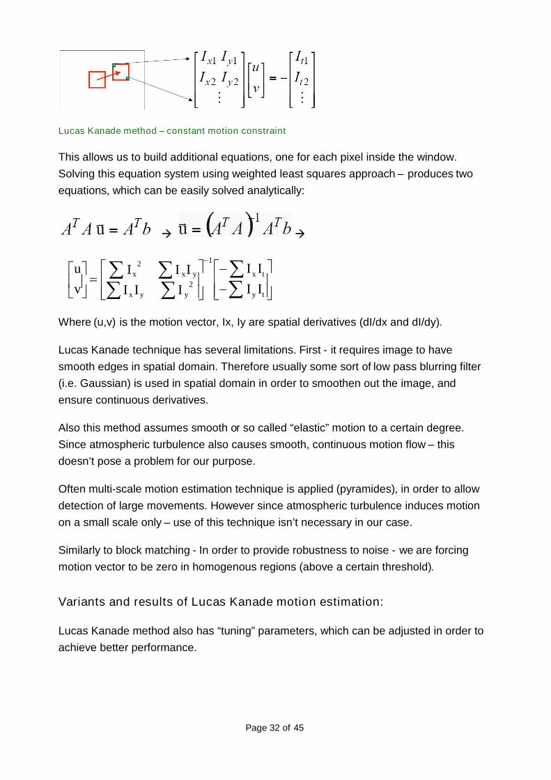
Lucas Kanade method – constant motion constraint
This allows us to build additional equations, one for each pixel inside the window.Solving this equation system using weighted least squares approach – produces twoequations, which can be easily solved analytically:
Where (u,v) is the motion vector, Ix, Iy are spatial derivatives (dI/dx and dI/dy).
Lucas Kanade technique has several limitations. First - it requires image to havesmooth edges in spatial domain. Therefore usually some sort of low pass blurring filter(i.e. Gaussian) is used in spatial domain in order to smoothen out the image, andensure continuous derivatives.
Also this method assumes smooth or so called “elastic” motion to a certain degree.Since atmospheric turbulence also causes smooth, continuous motion flow – thisdoesn’t pose a problem for our purpose.
Often multi-scale motion estimation technique is applied (pyramides), in order to allowdetection of large movements. However since atmospheric turbulence induces motionon a small scale only – use of this technique isn’t necessary in our case.
Similarly to block matching - In order to provide robustness to noise - we are forcingmotion vector to be zero in homogenous regions (above a certain threshold).
Variants and results of Lucas Kanade motion estimation:
Lucas Kanade method also has “tuning” parameters, which can be adjusted in order toachieve better performance.
ty
tx
yyx
yxx
IIII
IIIIII
vu
1
2
2
Page 33 of 45
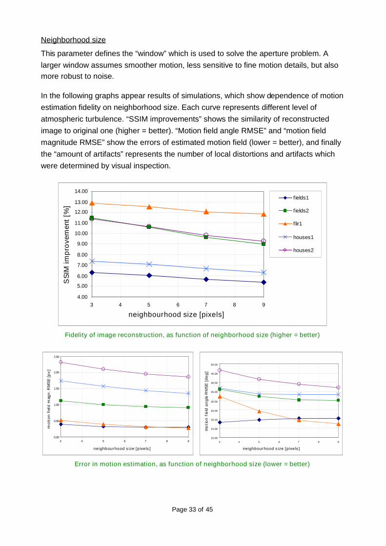
Neighborhood size
This parameter defines the “window” which is used to solve the aperture problem. Alarger window assumes smoother motion, less sensitive to fine motion details, but alsomore robust to noise.
In the following graphs appear results of simulations, which show dependence of motionestimation fidelity on neighborhood size. Each curve represents different level ofatmospheric turbulence. “SSIM improvements” shows the similarity of reconstructedimage to original one (higher = better). “Motion field angle RMSE” and “motion fieldmagnitude RMSE” show the errors of estimated motion field (lower = better), and finallythe “amount of artifacts” represents the number of local distortions and artifacts whichwere determined by visual inspection.
4.00
5.00
6.00
7.00
8.00
9.00
10.00
11.00
12.00
13.00
14.00
3 4 5 6 7 8 9
neighbourhood size [pixels]
SS
IMim
pro
vem
ent
[%]
f ields1
fields2
flir1
houses1
houses2
Fidelity of image reconstruction, as function of neighborhood size (higher = better)
Error in motion estimation, as function of neighborhood size (lower = better)
10.00
15.00
20.00
25.00
30.00
35.00
40.00
45.00
50.00
3 4 5 6 7 8 9
neighbourhood size [pixels]
mo
tio
nfi
eld
an
gle
RM
SE
[de
g]
0.00
0.50
1.00
1.50
2.00
2.50
3 4 5 6 7 8 9
neighbourhood size [pixels]
mo
tio
nfi
eld
mag
n.R
MS
E[p
x]
Page 34 of 45
0
1
2
3 4 5 6 7 8 9
neighbourhood size [pixels]
amo
unto
fart
efac
ts
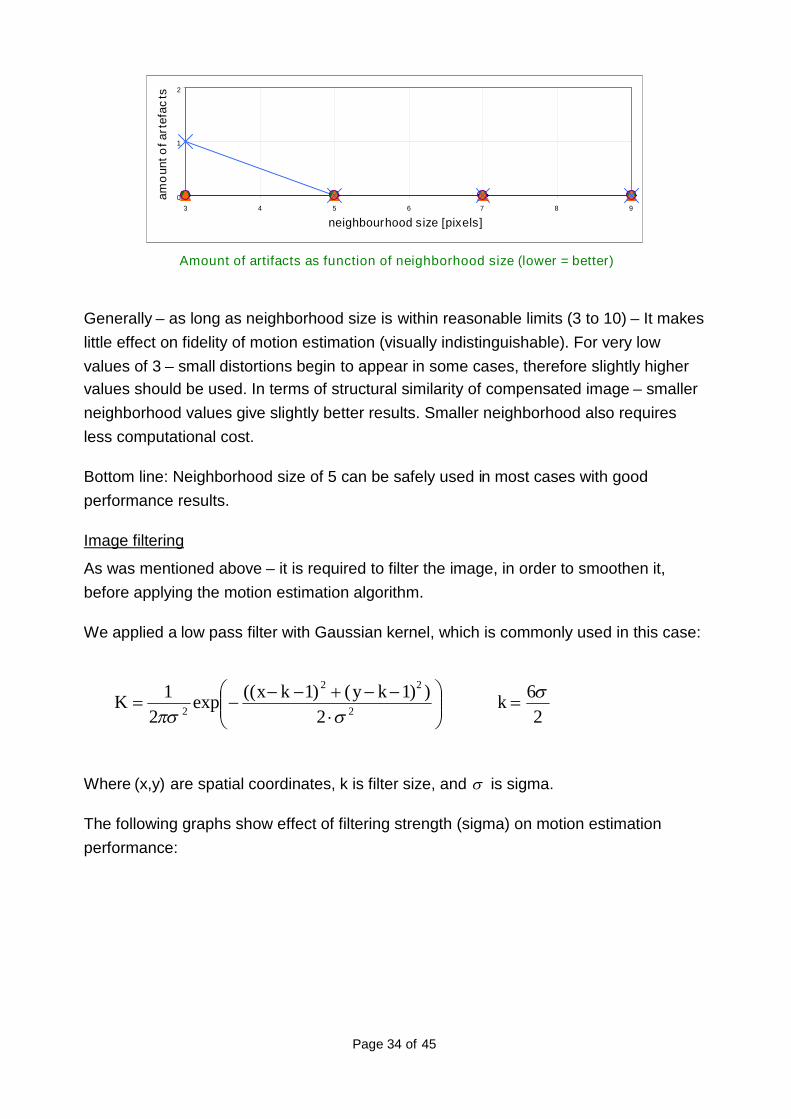
Amount of artifacts as function of neighborhood size (lower = better)
Generally – as long as neighborhood size is within reasonable limits (3 to 10) – It makeslittle effect on fidelity of motion estimation (visually indistinguishable). For very lowvalues of 3 – small distortions begin to appear in some cases, therefore slightly highervalues should be used. In terms of structural similarity of compensated image – smallerneighborhood values give slightly better results. Smaller neighborhood also requiresless computational cost.
Bottom line: Neighborhood size of 5 can be safely used in most cases with goodperformance results.
Image filtering
As was mentioned above – it is required to filter the image, in order to smoothen it,before applying the motion estimation algorithm.
We applied a low pass filter with Gaussian kernel, which is commonly used in this case:
Where (x,y) are spatial coordinates, k is filter size, and is sigma.
The following graphs show effect of filtering strength (sigma) on motion estimationperformance:
26
2))1()1((exp
21
2
22
2
kkykxK
Page 35 of 45
0.00
2.00
4.00
6.00
8.00
10.00
12.00
14.00
0.5 0.7 0.9 1.1 1.3 1.5 1.7 1.9
sigma
SS
IMim
pro
vem
ent[
%]
f ields1
fields2
flir1
houses1
houses2
Fidelity of image reconstruction, as function of image-filtering sigma (higher = better)
Error in motion estimation, as function of image-filtering sigma (lower = better)
0
1
2
0.5 0.7 0.9 1.1 1.3 1.5 1.7 1.9
sigma
am
ou
nt
of
arte
fac
ts
Amount of artifacts as function of image-filtering sigma (lower = better)
We can see that in terms of compensated image structural similarity – a sigma value of1 produces the best result for all cases of turbulence. Same happens in terms estimatedmotion field magnitude and angle errors. Visual inspection confirms that reconstructed
0.00
5.00
10.00
15.00
20.00
25.00
30.00
35.00
40.00
45.00
50.00
0.5 1 1.5 2sig ma
mot
ion
field
ang
leR
MSE
[deg
]
0.00
0.50
1.00
1.50
2.00
2.50
3.00
0.5 0.7 0.9 1.1 1.3 1.5 1.7 1.9
sigma
mot
ion
fiel
dm
agn.
RM
SE
[px]
Page 36 of 45
images with sigma value which is higher then 1 – differ significantly from the originalimage. For videos with extremely strong levels of turbulence – higher values of sigmagive us slightly “cleaner” images. However this effect is so small, that only extremecases should justify use of sigma value higher then 1.
Bottom line: In most cases: Gaussian kernel with sigma = 1 gives significantly betterresults then other values. In cases with extremely strong turbulence – use of slightlyhigher sigma value can be considered, in order to produce “cleaner” image, whilesacrificing the motion estimation accuracy.
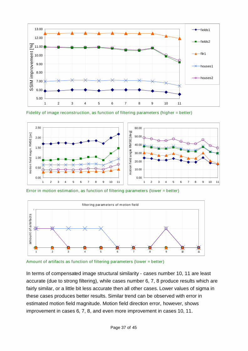
Filtering the motion field:
As opposed to block matching motion estimation – Lucas Kanade method producesmotion vector for each image pixel, and not only for each block. Since we assumeelastic and smooth motion – it can be beneficial to apply a low pass Gaussian filter onproduced motion field result.
Two filter parameters we can “play” with are sigma of the Gaussian kernel, and its size.These are results of simulations performed with different values of these parameters.The first graph displays variations of filter size and sigma, as a function of experimentserial number. The other graphs display performance evaluation of motion estimation asa function of the same experiment numbers.
0
3 3 3
5 5 5 5
10 10 10
00.5
2
4
0.51
3
5
0.5
2
4
0
2
4
6
8
10
12
1 2 3 4 5 6 7 8 9 10 11test number
motion filtersize
motion filtersigma
Motion field filtering parameters and experiment serial number
Page 37 of 45
5.00
6.00
7.00
8.00
9.00
10.00
11.00
12.00
13.00
1 2 3 4 5 6 7 8 9 10 11
SS
IMim
pro
vem
ent[
%]
f ields1
fields2
flir1
houses1
houses2
Fidelity of image reconstruction, as function of filtering parameters (higher = better)
Error in motion estimation, as function of filtering parameters (lower = better)
filtering parameters of motion field
0
1
2
1 2 3 4 5 6 7 8 9 10 11
amo
un
to
fart
efa
cts
Amount of artifacts as function of filtering parameters (lower = better)
In terms of compensated image structural similarity - cases number 10, 11 are leastaccurate (due to strong filtering), while cases number 6, 7, 8 produce results which arefairly similar, or a little bit less accurate then all other cases. Lower values of sigma inthese cases produces better results. Similar trend can be observed with error inestimated motion field magnitude. Motion field direction error, however, showsimprovement in cases 6, 7, 8, and even more improvement in cases 10, 11.
0.00
10.00
20.00
30.00
40.00
50.00
60.00
1 2 3 4 5 6 7 8 9 10 11
mot
ion
fiel
da
ngle
RM
SE
[de
g]
0.00
0.50
1.00
1.50
2.00
2.50
1 2 3 4 5 6 7 8 9 10 11
mo
tion
field
mag
n.R
MS
E[p
x]
Page 38 of 45
However due to small differences in terms of motion field estimation fidelity in all thesecases – main concern is achieving low amount of local distortions and artifacts. Visualinspection shows that for videos with weak turbulence – filtering the motion field doesn’tproduce big difference. However for videos with strong to very strong turbulence(“houses1” and “houses2”) – visual inspection revealed significant amount of distortionsand artifacts in most cases, except cases number 6, 7, 8 (with filter kernel size = 5) andcases number 10, 11 (with kernel size 10 and sigma 2 and 4 respectfully) whichproduced clean images.
Bottom line:Filtering the motion field improves the compensated image in terms of distortions andartifacts, and recommended values for Gaussian filter kernel are: size=5 and sigma=1.For images with especially strong turbulence: consider using larger kernel (10) withlarger sigma (2-4).
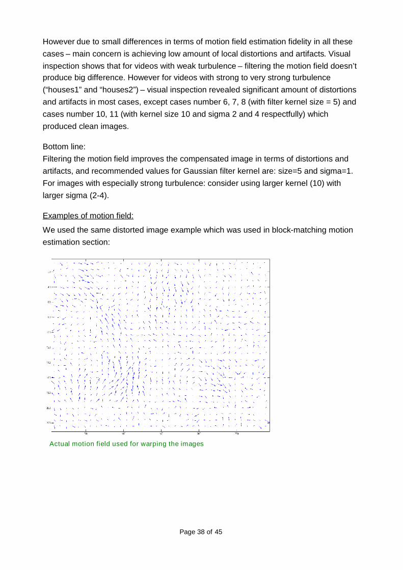
Examples of motion field:
We used the same distorted image example which was used in block-matching motionestimation section:
Actual motion field used for warping the images
Page 39 of 45
Estimated motion field, using Lucas Kanade method, no motion field filtering
Estimated motion field, using Lucas Kanade method, strong motion field filtering
Examples of compensated images:
Video with weak turbulence (fields 1):
Page 40 of 45
Distorted frame (t = T1)
Original frame (t = 0)
Compensated image with parameter set which gives best results for LK method
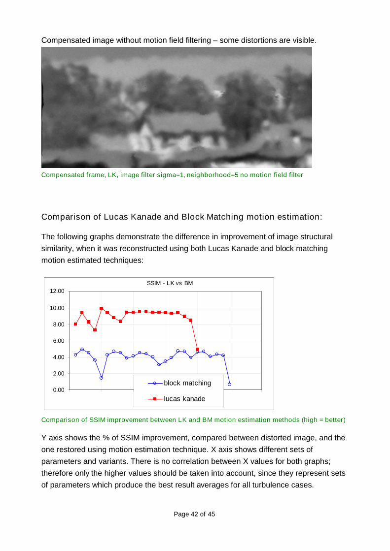
Compensated image without motion field filtering – some distortions are visible.
Compensated frame, LK, image filter sigma=1, neighborhood=5 no motion field filter
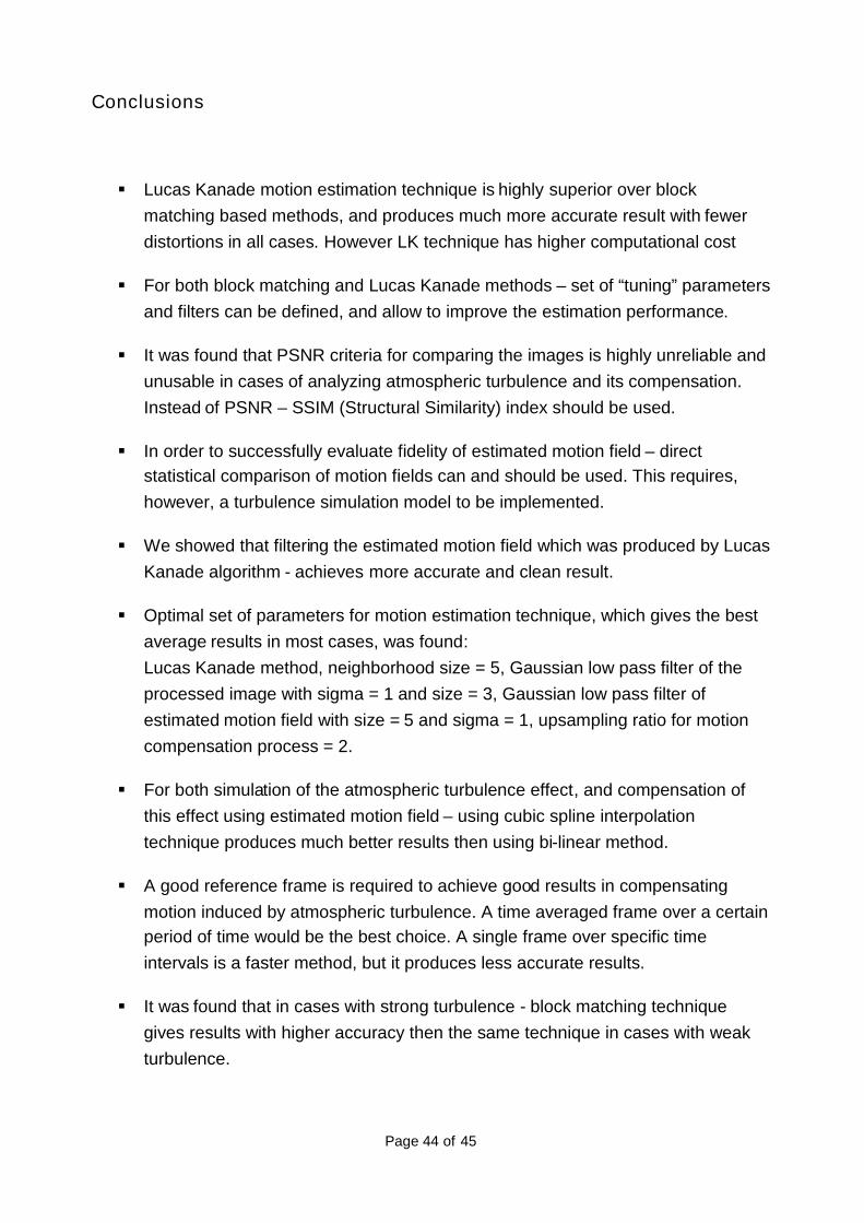
Comparison of Lucas Kanade and Block Matching motion estimation:
The following graphs demonstrate the difference in improvement of image structuralsimilarity, when it was reconstructed using both Lucas Kanade and block matchingmotion estimated techniques:
SSIM - LK vs BM
0.00
2.00
4.00
6.00
8.00
10.00
12.00
0 5 10 15 20 25 30
block matching
lucas kanade
Comparison of SSIM improvement between LK and BM motion estimation methods (high = better)
Y axis shows the % of SSIM improvement, compared between distorted image, and theone restored using motion estimation technique. X axis shows different sets ofparameters and variants. There is no correlation between X values for both graphs;therefore only the higher values should be taken into account, since they represent setsof parameters which produce the best result averages for all turbulence cases.
Page 43 of 45
It is clear that Lucas Kanade technique in most of its variants – produces superiorresults which are approximately twice as accurate as block matching method.
Note that last result, which shows significant drop of SSIM improvement in both cases –is the case where no upsampling for motion compensation was used to achieve sub-pixel accuracy. This clearly shows importance of performing it.
The following graphs display comparison of magnitude, and the angle errors betweenLK and BM motion estimation techniques:
motion magnitude RMSE - LK vs BM
0.00
0.501.00
1.502.00
2.503.00
3.50
4.004.50
0 5 10 15 20 25 30block matching
lucas kanade
Comparison of errors in motion field magnitude errors between LK and BM methods (low = better)
motion angle RMSE - LK vs BM
0.0010.0020.0030.0040.0050.0060.0070.0080.0090.00
0 5 10 15 20 25 30
block matching
lucas kanade
Comparison of errors in motion field direction errors between LK and BM methods (low = better)
We can see that in this case also – Lucas Kanade technique is superior to blockmatching, and produces much less errors both in direction of estimated motion vectors,and in their magnitudes.
Page 44 of 45
Conclusions
Lucas Kanade motion estimation technique is highly superior over blockmatching based methods, and produces much more accurate result with fewerdistortions in all cases. However LK technique has higher computational cost
For both block matching and Lucas Kanade methods – set of “tuning” parametersand filters can be defined, and allow to improve the estimation performance.
It was found that PSNR criteria for comparing the images is highly unreliable andunusable in cases of analyzing atmospheric turbulence and its compensation.Instead of PSNR – SSIM (Structural Similarity) index should be used.
In order to successfully evaluate fidelity of estimated motion field – directstatistical comparison of motion fields can and should be used. This requires,however, a turbulence simulation model to be implemented.
We showed that filtering the estimated motion field which was produced by LucasKanade algorithm - achieves more accurate and clean result.
Optimal set of parameters for motion estimation technique, which gives the bestaverage results in most cases, was found:Lucas Kanade method, neighborhood size = 5, Gaussian low pass filter of theprocessed image with sigma = 1 and size = 3, Gaussian low pass filter ofestimated motion field with size = 5 and sigma = 1, upsampling ratio for motioncompensation process = 2.
For both simulation of the atmospheric turbulence effect, and compensation ofthis effect using estimated motion field – using cubic spline interpolationtechnique produces much better results then using bi-linear method.
A good reference frame is required to achieve good results in compensatingmotion induced by atmospheric turbulence. A time averaged frame over a certainperiod of time would be the best choice. A single frame over specific timeintervals is a faster method, but it produces less accurate results.
It was found that in cases with strong turbulence - block matching techniquegives results with higher accuracy then the same technique in cases with weakturbulence.
Page 45 of 45
References
[1] Li, Dalong, et al. "New method for suppressing optical turbulence in video." Proceedings ofthe European Signal Processing Conference (EUSIPCO). 2005.
[3] Barreto, Dacil, L. D. Alvarez, and J. Abad. "Motion estimation techniques in super-resolutionimage reconstruction a performance evaluation." Virtual Observatory. Plate Content
Digitalization, Archive Mining and Image Sequence Processing (2005): 254-268.
[4] Li, Dalong, Russell M. Mersereau, and Steven Simske. "Blur identification based on kurtosis
minimization." Image Processing, 2005. ICIP 2005. IEEE International Conference on. Vol. 1.IEEE, 2005.
[5] Gepshtein, Shai, et al. "Restoration of atmospheric turbulent video containing real motionusing rank filtering and elastic image registration." Proceedings of the 12th European SignalProcessing Conference (EUSIPCO). 2004.
[6] Shimizu, Masao, et al. "Super-resolution from image sequence under influence of hot-airoptical turbulence." Computer Vision and Pattern Recognition, 2008. CVPR 2008. IEEE
Conference on. IEEE, 2008.
[7] Hayakawa, Hitoshi, and Tadashi Shibata. "Block-matching-based motion field generation
[9] Quirrenbach, Andreas. "The effects of atmospheric turbulence on astronomicalobservations." A. Extrasolar planets. Saas-Fee Advanced Course 31 137 (2006): 137.
[10] Burger, Liesl, Igor A. Litvin, and Andrew Forbes. "Simulating atmospheric turbulence using
a phase-only spatial light modulator." South African Journal of Science 104.3-4 (2008): 129-134.