Evaluation of PM2.5 Chemical Speciation Samplers for Use ... · Evaluation of PM 2.5 Chemical...

United States Office of Air Quality EPA-454/R-01-005Environmental Protection Planning and Standards NTIS PB#2001-105814Agency Research Triangle Park, NC 27711 Date: May 2001

Air

Evaluation of PM2.5 ChemicalSpeciation Samplers for Use inthe EPA National PM2.5

Chemical Speciation Network

Evaluation of PM2.5 Chemical Speciation Samplers for Use in the EPANational PM2.5 Chemical Speciation Network

Volume I – Introduction, Results, and Conclusions

Final Report

15 July 2000

Prepared By

Paul A. SolomonWilliam MitchellMichael Tolocka

Gary NorrisDavid GemmillRussell Wiener

US EPAOffice of Research and Development

National Exposure Research LaboratoryResearch Triangle Park, NC 27711

Robert VanderpoolRobert MurdochSanjay Natarajan

Eva HardisonResearch Triangle Institute

Research Triangle Park, NC 27711

Prepared for

Richard ScheffeJames Homolya

Joann RiceOffice of Air Quality Planning and Standards

Research Triangle Park, NC

Part I, Page i

DISCLAIMER

This work has been funded wholly or in part by the United States Environmental Protection Agency. Portions of the work were performed under Contract No. 68-D5-0040 by Research Triangle Institute. It has been subjected to Agency review and approved for publication. Mention of trade names orcommercial products does not constitute an endorsement or recommendation for use.

Part I, Page ii

ACKNOWLEDGMENTS

The authors would like to thank the many people who assisted in the design, implementation, dataanalysis, and preparation of this final report. In particular, the authors would like to thank, Mel Zeldin(SCAQMD) and Tom Moore (Arizona DEQ) for providing space, operational support, logistics, andpower at the Rubidoux and Phoenix air monitoring sites, respectively. We would also like to thank thesite operators at Rubidoux and Phoenix for their long hours and their dedication to the project. We arealso grateful to the RTI staff who operated the Philadelphia and RTP sites and performed the fieldaudits and those that spent many long hours changing filters and performing chemical analysis. We arealso appreciative of Judy Chow and her staff (DRI), Bob Cary and his staff (Sunset Labs), and BobKellogg (Mantech) for analyzing filters with a very quick turn around time. The project would not havebeen successful without the assistance of the manufacturer’s representatives, Tom Merrifield (MetOne),Wes Davis (Andersen), and Jon Stone (URG) and their willingness to help train and set up thesamplers, and their prompt response to problems encountered during sampling. Thanks is also given toLowell Ashbaugh of UC Davis who supplied the IMPROVE samplers for this study. We are indebtedto Jack Suggs (EPA, ORD) for his assistance with the statistical analysis effort described in this report. The PM Expert Panel reviewed the program plan and provided valuable assistance in their first reviewof the Speciation Guidance Document with the initial recommendations for having this evaluation study. Finally, we thank our clients at the Office of Air Quality Planning and Standards, and in particular,James Homolya, Joann Rice, Shelly Eberly, and Richard Scheffe. Their support and assistancethroughout the study was indispensable, as well as support from Russell Wiener, Branch Chief,AMMB. This project was supported by funds from the OAQPS speciation program and fromORD/NERL/HEASD/AMMB PM Methods Team.

Part I, Page iii

EXECUTIVE SUMMARY

To develop improved source-receptor relationships and for better understanding the causes of highPM2.5 concentrations in the atmosphere, it is necessary to not only determine concentrations of PM2.5

mass, the NAAQS indicator, but also the chemical components of PM2.5. A sampling program of thistype, which will consist of up to 300 sites nationwide has been initiated by EPA (Speciation GuidanceDocument, 1999 at http://www.epa.gov/ttn/amtic/pmspec.html). Since the PM2.5 Federal ReferenceMethod (FRM) using only Teflon filters is not suitable for determining the chemical composition of thecollected aerosol, since carbon can not be directly measured (Speciation Guidance Document, 1999),EPA solicited innovative designs for speciation samplers, based on performance specifications. Thisled to the development of three slightly different candidate samplers manufactured by AndersenInstrument Inc., MetOne, Inc., and University Research Glassware (URG). These samplers aredesigned to allow for a nearly complete mass balance of the collected aerosol, while minimizingsampling artifacts for nitrate and allowing flexibility for minimizing organic carbon artifacts in the future. Due to the need to have consistency across this national network, the Speciation Expert Panel(Recommendations of the 1998 Expert Panel, 1998 at http://www.epa.gov/ttn/amtic/ pmspec. html)recommended a methods comparison field study among the new speciation samplers, historically usedsamplers, and the PM2.5 FRM. The program plan for EPA’s Chemical Speciation Sampler EvaluationStudy (1999, http://www.epa. gov/ttn/amtic/casacinf.html) details the approach and implementation ofthe study. This report presents the approach and results from the 4-City intercomparison study; Phase1, of the full evaluation of these samplers. Other Phases are described in Field Program Plan (1999)and include evaluation of denuders and reactive post filters for sampling organic aerosols with minimalartifacts (Phase II, Seattle, WA, J. Lewtas, PI), an evaluation of the chemical speciation samplers undersummertime conditions (Phase II, Atlanta, GA in conjunction with the Atlanta Supersites Program, P.Solomon, PI), and an evaluation of the samplers under a variety of environmental conditions to testoperational performance and logistics with the National Chemical Speciation Laboratory (Phase IV, 15Cities throughout the US (Mini-trends network, J. Homolya, PI).

Methods. Because of potential sampling artifacts when using filters and potential differences in inletcutpoints and sample fractionators, the chemical speciation samplers must be able to properlydetermine the chemical components of PM2.5 under a variety of atmospheric and environmentalconditions. Four locations, with different atmospheric chemical and meteorological conditions werechosen and included: Rubidoux, CA (high nitrate and carbon and low sulfate), Phoenix, AZ (highcrustal material and moderate carbon and nitrate), Philadelphia, PA (high sulfate, moderate carbon, andlow nitrate), and Research Triangle Park (RTP), NC (low PM2.5 concentrations). The latter site alsoallowed for a more thorough evaluation of the samplers’ in-field operational performance as it waslocated near EPA offices in RTP. In addition to the three candidate samplers, a Versatile Air PollutionSampler (VAPS), an IMPROVE sampler, and an FRM were collocated at each site. Replicatesamplers were located at Rubidoux. Samples were collected for up to 20 days during January andFebruary, 1999 using state personnel (Rubidoux and Phoenix) or EPA contractors (Philadelphia andRTP). All sampling periods were 24-hrs in duration. Mass and trace elements were determined on

Part I, Page iv

Teflon filters; sulfate, nitrate, and ammonium were determined on either Teflon, pre-fired quartz-fiber,or nylon filters depending on the sampler; and OC/EC were determined on pre-fired quartz-fiber filters. To minimize variability, all filter preparation, filter changing, and chemical analyses for a particularspecies were performed by one contractor. Quality assurance/quality control followed EPA guidelines(QAPP for the Four-City PM2.5 Chemical Speciation Sampler Evaluation Study, January, 1999Research Triangle Institute, Project Number 07263-030).

Results. All samplers encountered operational problems that increased variability in the results;however, the Andersen and MetOne samplers collected over 90% of the attempted samples on a site-by-site basis successfully, while the URG and Versatile Air Pollution Sampler (VAPS) collected greaterthen 75% of the samples attempted on a site-by-site basis. Most manufacturers have resolvedoperational issues. Other minor engineering changes were made to two of the samplers after the study,to allow for easier operation in the field. A fundamental problem was noted early on with the MetOnespiral inlet, which was allowing particles greater then 2.5 Fm to penetrate the inlet. The spiral inlet hasbeen replaced with a sharp cut cyclone.

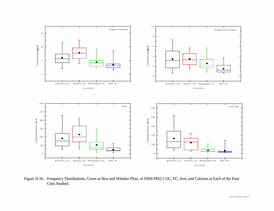
Chemical composition of the aerosols at each site were within expectations with the exception of highnitrate and OC in Philadelphia, where nitrate and sulfate both were about 20% of the total PM2.5 massand OC was about 50%. Results from most studies in the eastern US indicate that sulfate is the highestspecies (~50% of the mass), followed by OC at about 30% of the mass, with nitrate accounting for lessthan 5% or so of the mass. However, most previous studies have occurred during the summertime,when temperatures are high and ammonium nitrate would be mostly in the gas phase. Finally, coarseparticle concentrations were highest in Phoenix and Rubidoux (about equal to the fine particle mass)and only about 20% or less relative to the fine particle mass at Philadelphia and RTP, as expected. Therefore, this study met its objective of testing the chemical speciation samplers under a fairly widerange of chemical conditions.

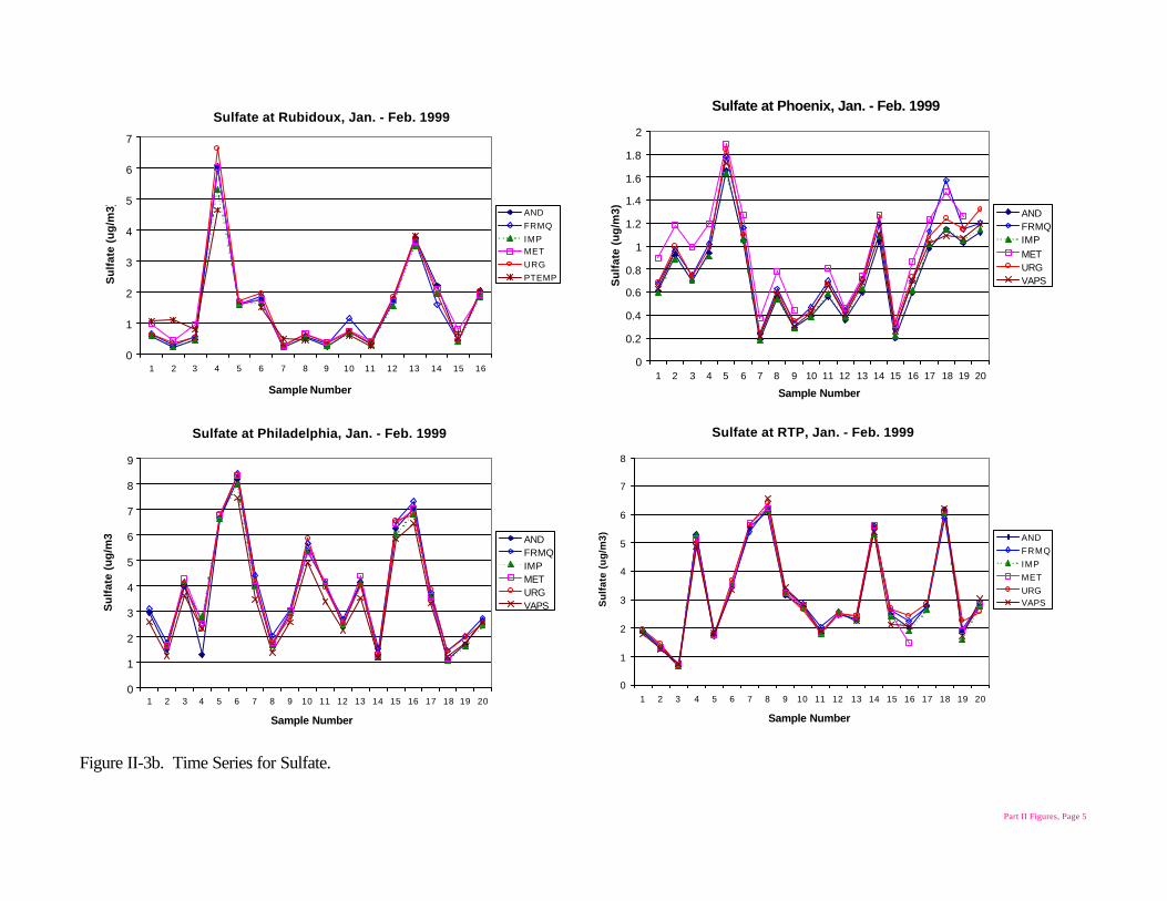
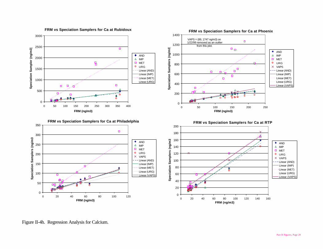
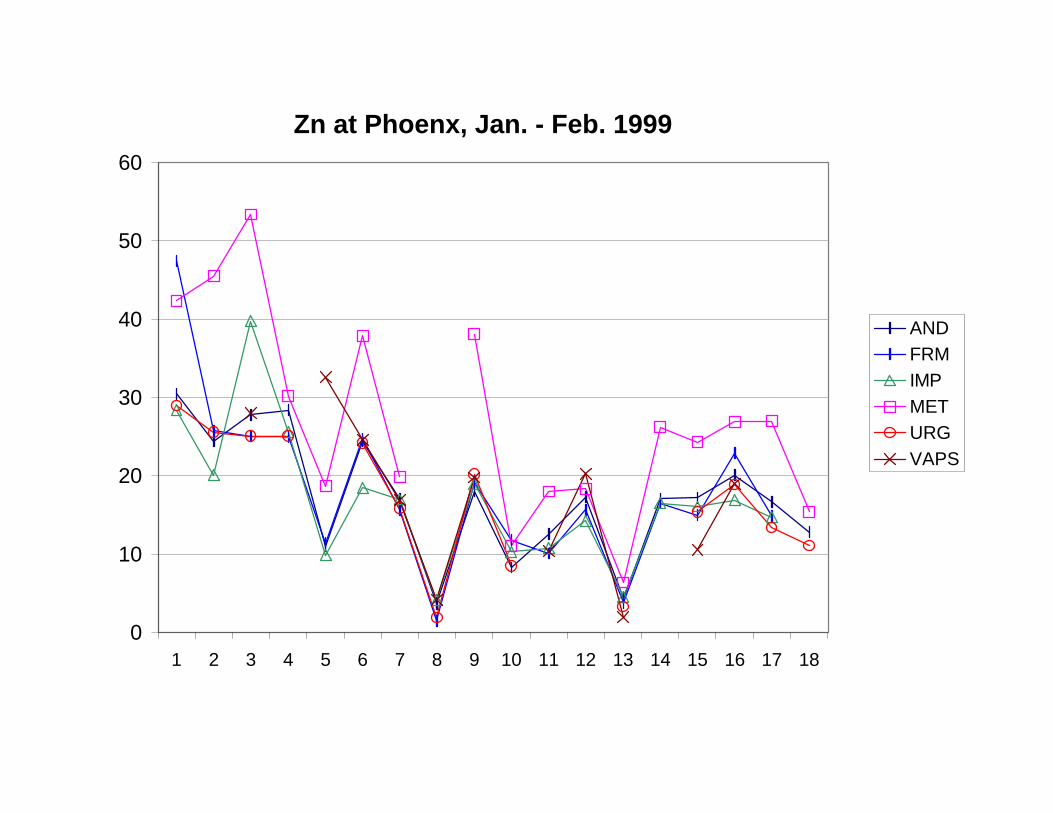
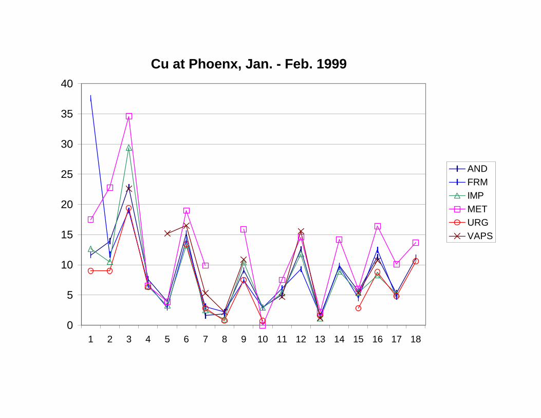
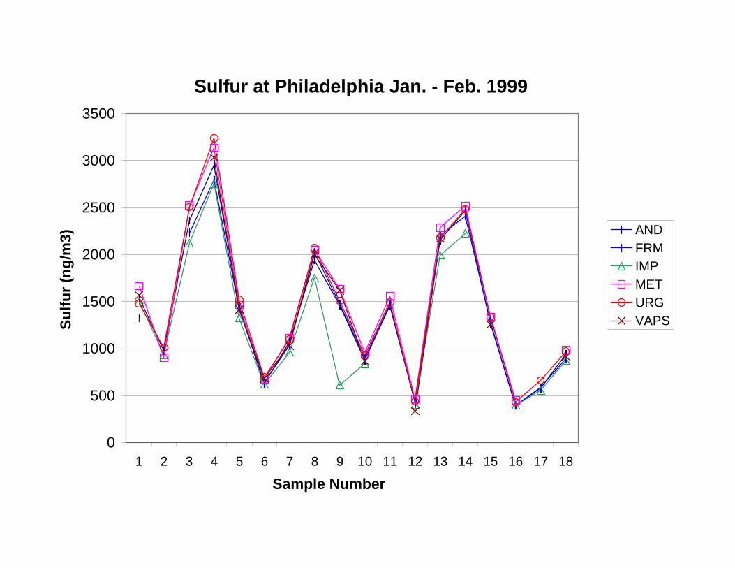
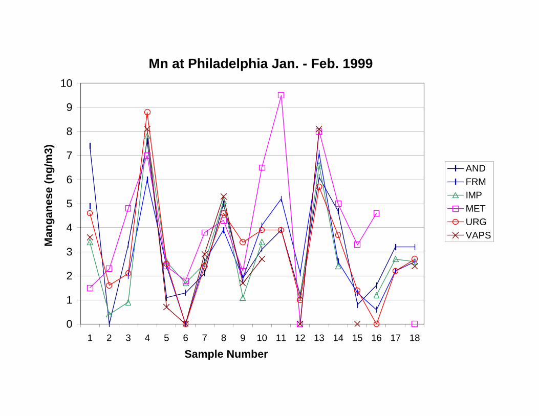
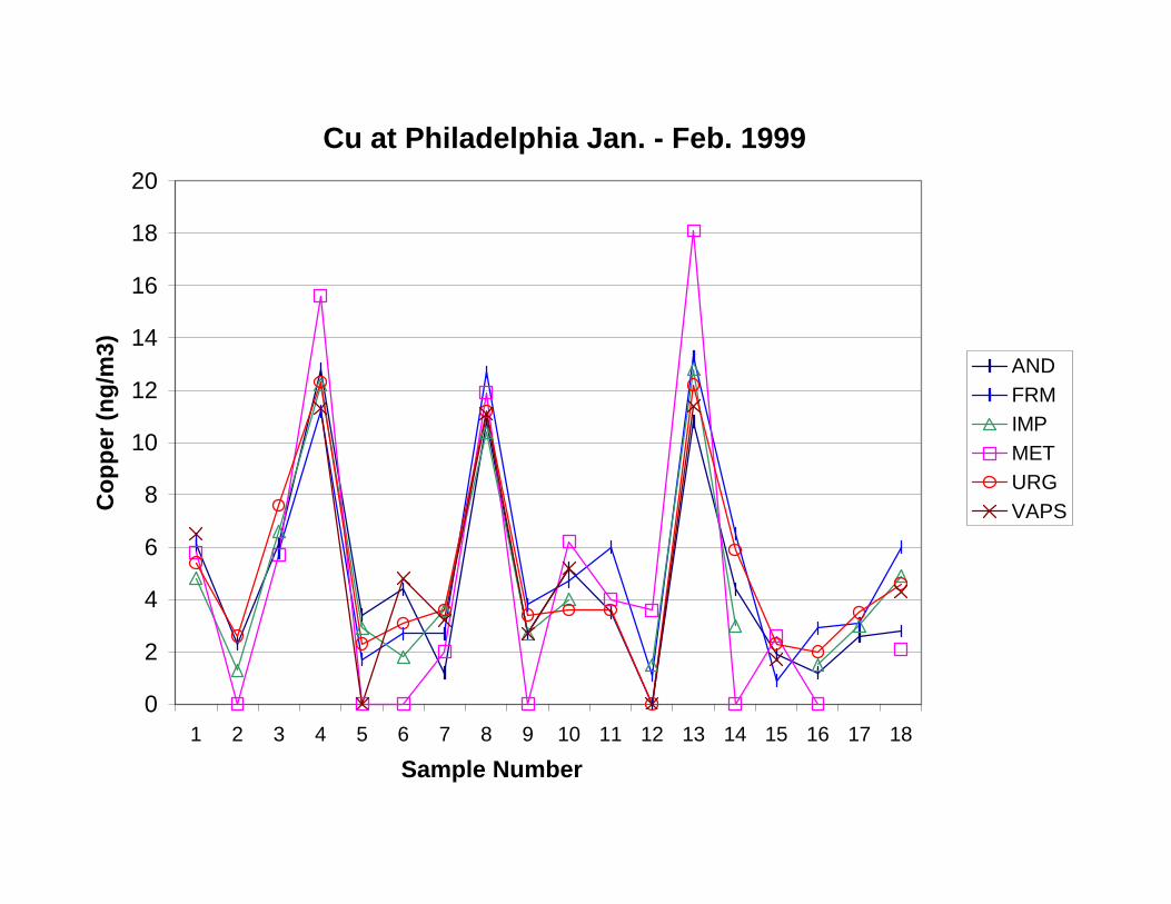
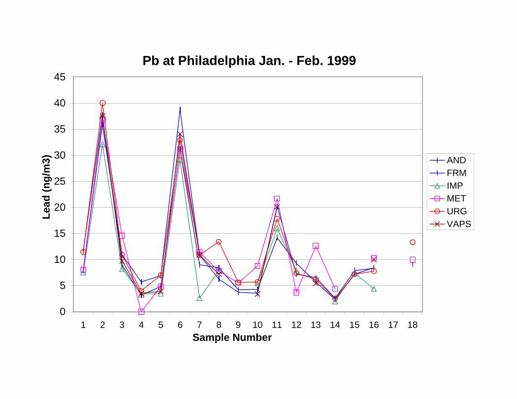
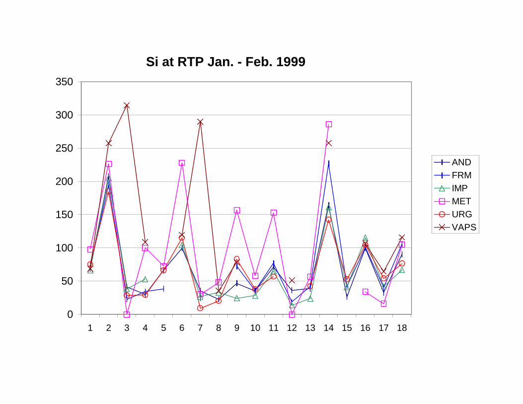
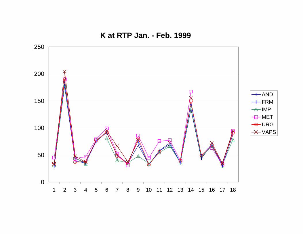
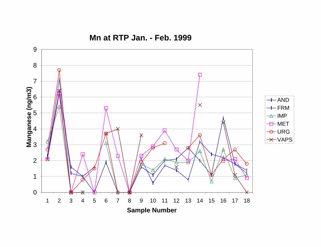
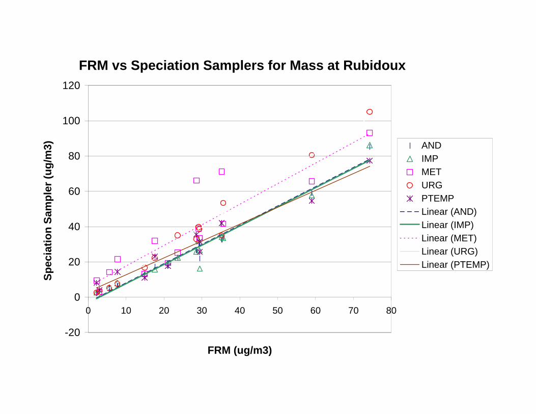
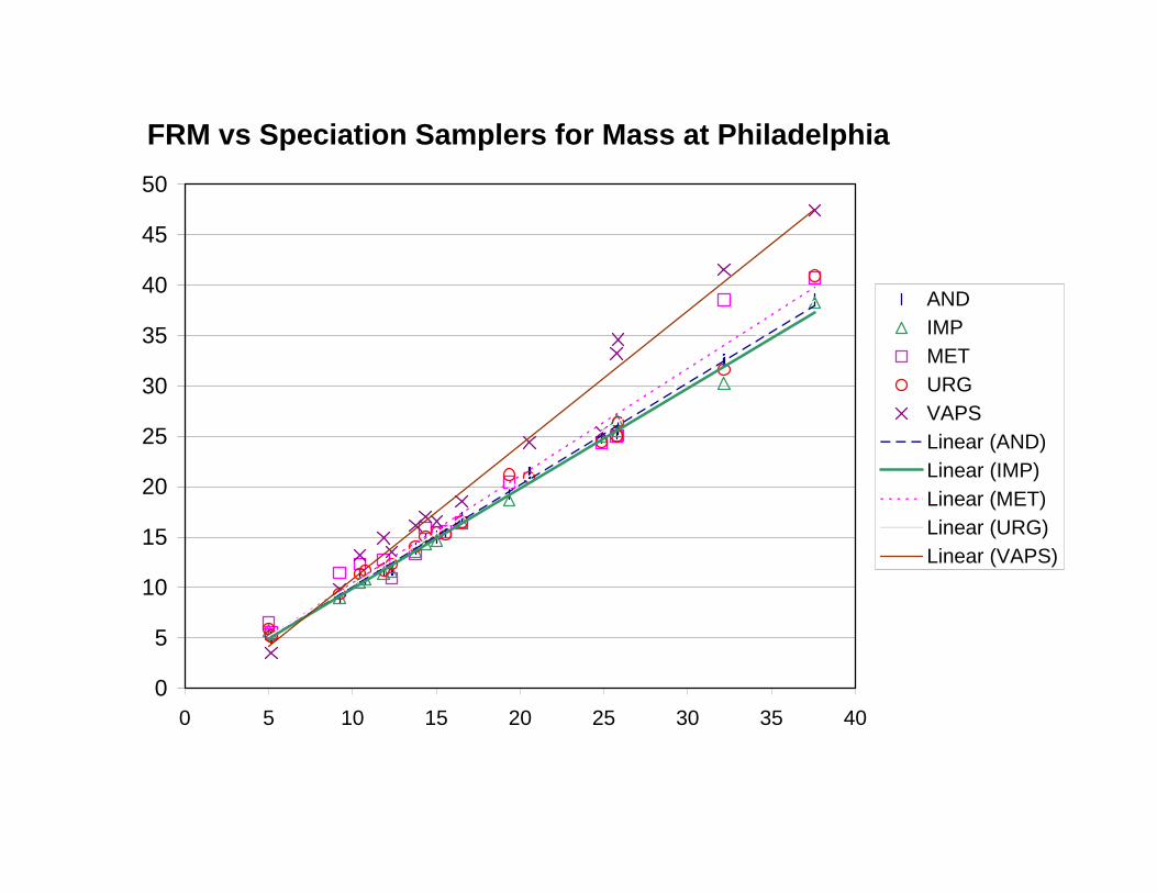
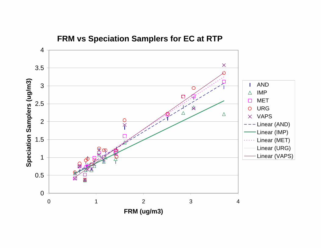
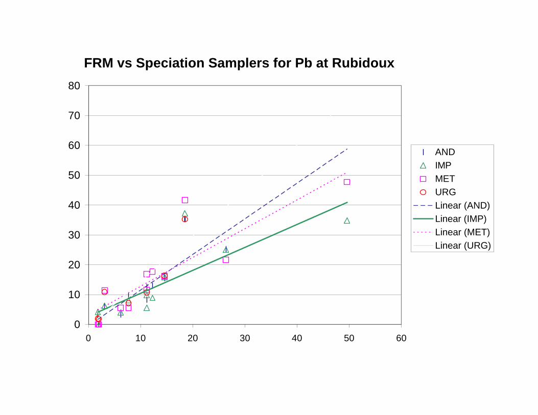
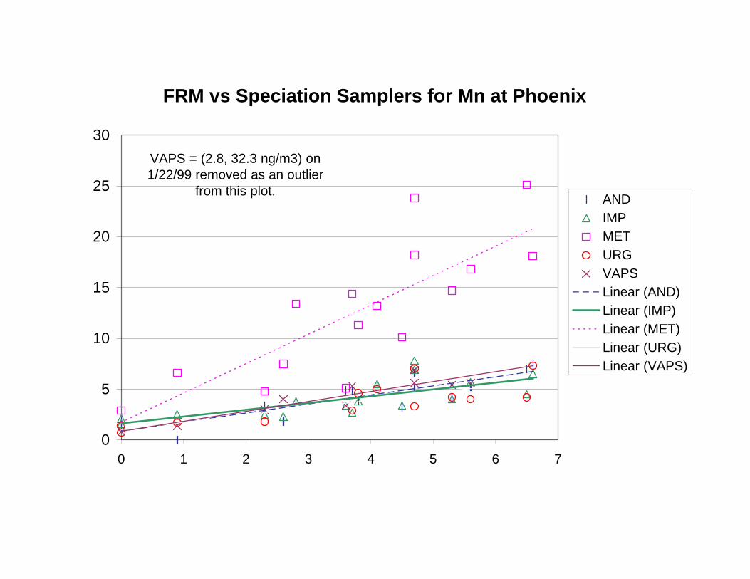
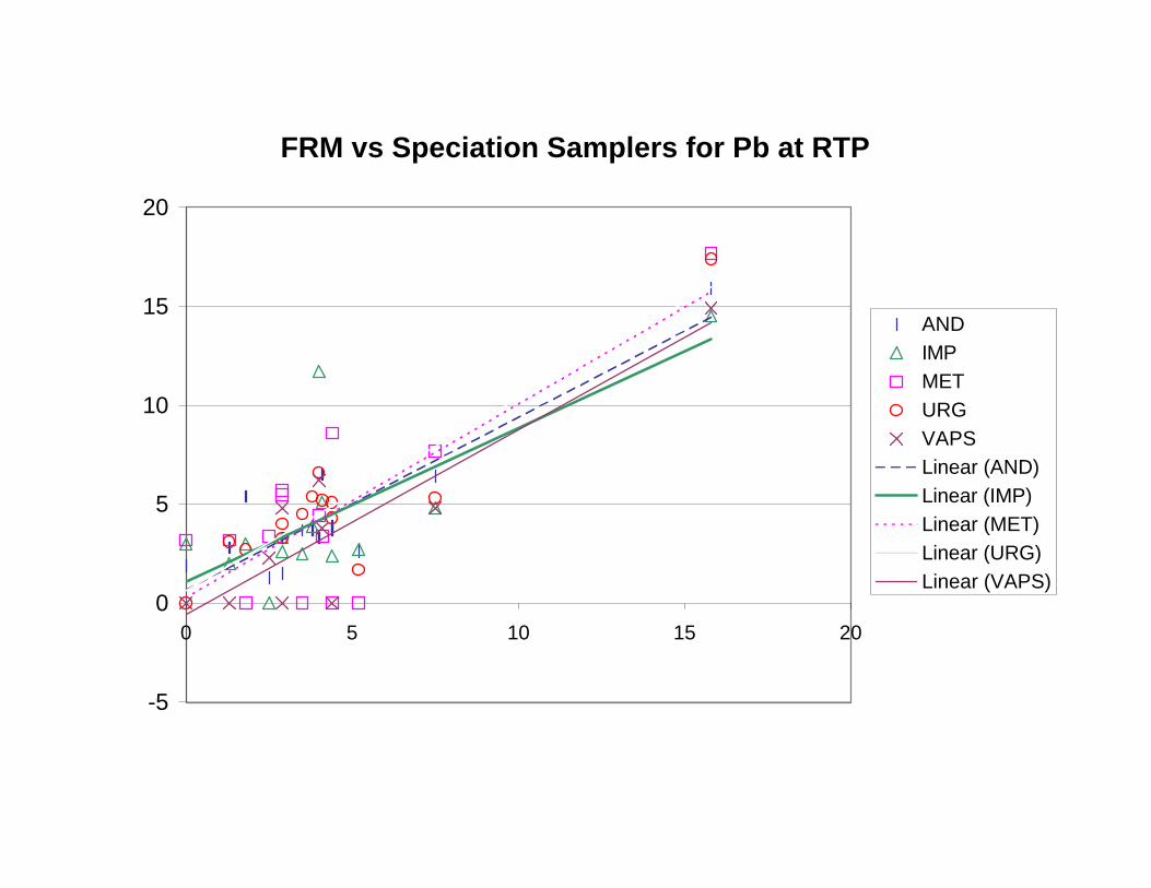
Means, time series, and regression analyses were performed for all species measured, allowingcomparison among the samplers for a given variable at a given site. On the average, the major speciesagreed within 10-15% among the FRM, Andersen, and Improve samplers. Sulfate had even betteragreement, which was observed across all samplers. The MetOne and VAPS samplers tended to behigh for species that normally have a coarse particle component (i.e., mass, Si, Fe, Ca, etc.). In general,individual species from all samplers tracked each other, with the majority of correlation coefficients (r)being greater then 0.85. A few exceptions were noted. More variability was observed for traceelements (Si, K, Ca, Fe, Cu, Zn, Pb, and As).

Differences, on the order of up to 1 µg/m3 on the average were observed among the samplers forparticle nitrate due to a possible positive artifact associated with determining nitrate on pre-fired quartz-fiber filters, which usually is not observed with quartz-fiber filters that have not been pre-treated (Chow,1995 JAWMA 45, 320). The quartz-fiber filter was used due to concerns regarding loss of nitrateduring vacuum XRF analysis (i.e., XRF has to be performed before the filter is extracted for ionsanalysis). Tests comparing nitrate concentrations measured on Teflon filters, collected in parallel, with

Part I, Page v

and without having vacuum XRF analysis indicated loss of up to 40% of the nitrate, assumed to beammonium nitrate. An additional bias for collecting particulate nitrate was observed due to the methodof collecting particulate nitrate, where nitrate concentrations determined by the direct method (nitratemeasured directly on a filter behind a denuder) were up to 1.5 µg/m3 lower than nitrate concentrationsmeasured by the indirect method (nitrate measured on a quartz-fiber filter behind a denuder and Teflonfilter plus nitrate measured on a quartz-fiber filter in parallel).

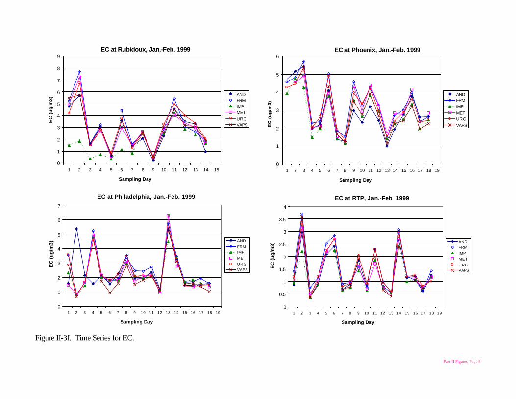
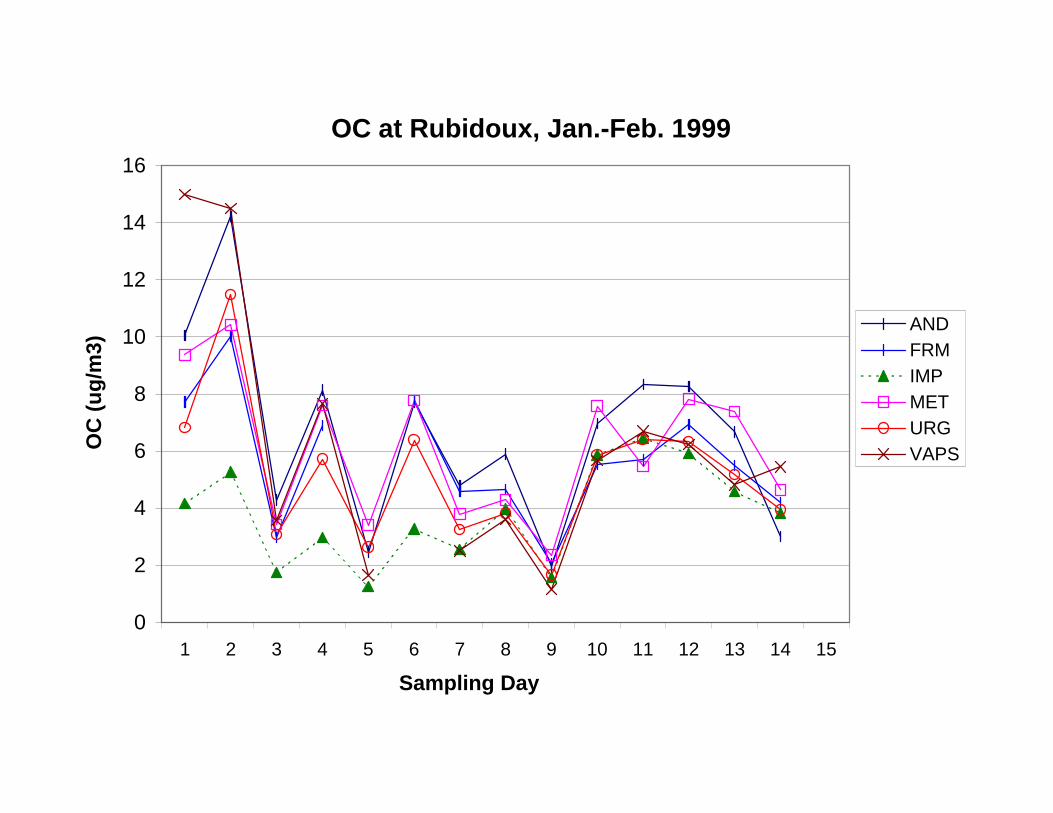
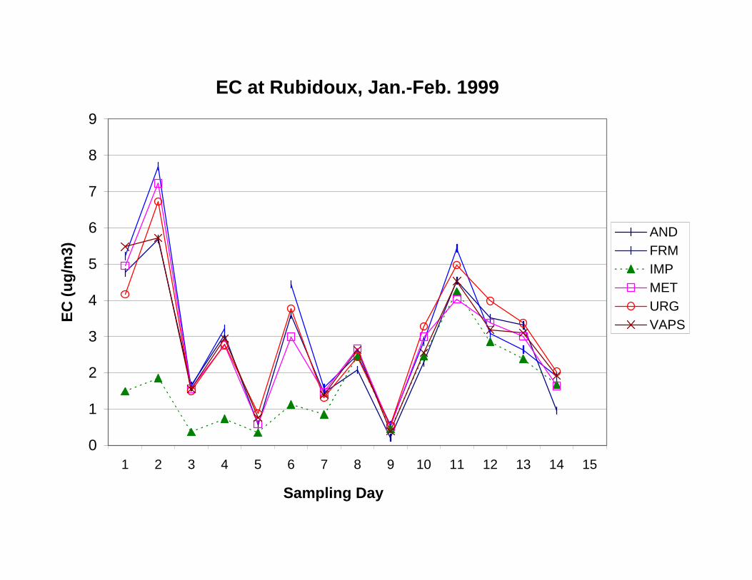
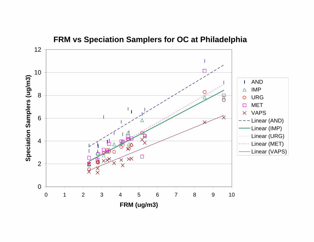
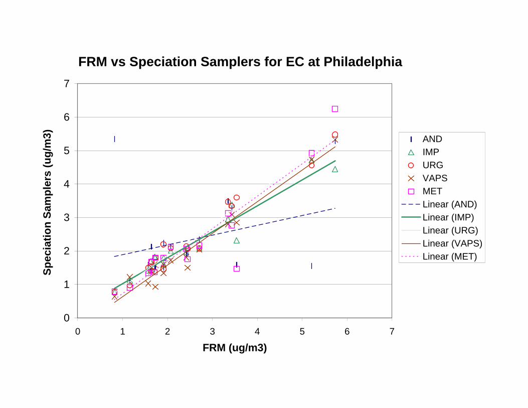
Differences also were observed among the samplers for organic carbon and appear to be due to filterface velocity variations among the samplers. Lower flow rates appear to result in higher OCconcentrations; although EC is consistent among the samplers. A positive artifact was also noted forOC and ranged from about 3.5 µg/m3 at Rubidoux to essentially zero at RTP. Based on the design ofthe study, no information can be implied about OC negative artifacts, but the assumption has been madein the above discussion that negative artifacts for OC are similar between Teflon and quartz-fiber filtersoperating at the same face velocity.

Differences were observed between EC values reported the IMPROVE OC/EC protocol versus theNIOSH protocol. The IMPROVE protocol reported EC values approximately 2 times higher then theNIOSH method. These differences are currently under investigation.

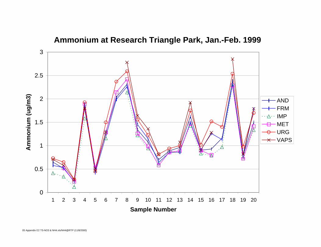
Ammonium ion as measured by the IMPROVE sampler was on average lower than on the othersamplers, even though a similar bias was not observed for nitrate or sulfate. It is postulated thatammonium is being lost due to volatilization of the ammonium nitrate that is collected on the nylon filter inthe IMPROVE sampler. While nitric acid volatilized from the collected ammonium nitrate would becollected by the basic (pH) nylon filter, ammonia would not be collected. It also is possible that thebasic filter is enhancing ammonium volatilization. More careful experiments need to be conducted toestablish if this potential bias is significant or not.

Conclusions. In general, the performance of the candidate samplers is reasonable for their first use inthe field. All samplers had operational problems that increased their variability, most of which have beenaddressed by the manufactures. Tradeoffs exist among the samplers for ease of use, flexibility forsampling, and cost. Performance of the samplers was excellent for sulfate and reasonable for otherstable species. However, real differences among the samplers exist for nitrate and organic carbon andpossibly ammonium as collected in the IMPROVE sampler. These differences are significant and canpossibly affect design of compliance strategies for controlling PM2.5 mass concentrations in air, as totaldifferences as high as 3-5 µg/m3 are observed among the samplers for these two species. Results fromthis study yield the following recommendations for the collection of nitrate and organic carbon:

• The Teflon filter used for mass and XRF analysis should not be used for ions analysis,particularly nitrate and ammonium ions, as these species are lost during XRF analysis.

Part I, Page vi

• To minimize artifacts for the collection of aerosol nitrate, it should be measured using a denuder(coated with MgO or Na2CO3) followed by a single filter (Nylasorb or Na2CO3). Measuringnitrate on a quartz-fiber filter prepared for carbon analysis can results in a significant (1-3 µg/m3)positive artifact for aerosol nitrate, after accounting for volatilized nitrate measured on a nylonfilter behind a denuder and Teflon filter.

• Organic carbon should be measured at the same face velocity as the Federal ReferenceMethod. This will result in similar negative biases between OC measured on a quartz-fiber filterand that of a Teflon filter. Positive biases were observed on the quartz-fiber filter collectingaerosol directly behind a PM2.5 inlet relative OC measured behind the same inlet that is followedby an XAD-4 coated annular denuder. It is recommended that the speciation networkeventually consider use of an XAD-4 denuder or similar denuder for removing potential gasphase artifacts followed by a quartz-fiber filter and a reactive backup filter to obtain OC withminimal bias.

Part I, Page vii

TABLE OF CONTENTS – Volume 1: PARTS I AND II

VOLUME I: INTRODUCTION, RESULTS, AND CONCLUSIONS

DISCLAIMER . . . . . . . . . . . . . . . . . . . . . . . . . . . . . . . . . . . . . . . . . . . . . . . . . . . . . . Part I, Page i

ACKNOWLEDGMENTS . . . . . . . . . . . . . . . . . . . . . . . . . . . . . . . . . . . . . . . . . . . . . Part I, Page ii

EXECUTIVE SUMMARY . . . . . . . . . . . . . . . . . . . . . . . . . . . . . . . . . . . . . . . . . . . . Part I, Page iii

TABLE OF CONTENTS – PARTS I AND II . . . . . . . . . . . . . . . . . . . . . . . . . . . . . Part I, Page vii

List of Tables – Parts I and II . . . . . . . . . . . . . . . . . . . . . . . . . . . . . . . . . . . . . . . . . Part I, Page xi

List of Figures – Parts I and II . . . . . . . . . . . . . . . . . . . . . . . . . . . . . . . . . . . . . . . . . Part I, Page xiii

List of Appendices – Parts I and II . . . . . . . . . . . . . . . . . . . . . . . . . . . . . . . . . . . . Part I, Page xiv

Part I: Introduction and Experimental Design

INTRODUCTION . . . . . . . . . . . . . . . . . . . . . . . . . . . . . . . . . . . . . . . . . . . . . . . . . . . Part I, Page 2About this Report . . . . . . . . . . . . . . . . . . . . . . . . . . . . . . . . . . . . . . . . . . . . . . . . Part I, Page 2Study Objectives . . . . . . . . . . . . . . . . . . . . . . . . . . . . . . . . . . . . . . . . . . . . . . . . Part I, Page 3Overview of the Intercomparison . . . . . . . . . . . . . . . . . . . . . . . . . . . . . . . . . . . . Part I, Page 3Study Design . . . . . . . . . . . . . . . . . . . . . . . . . . . . . . . . . . . . . . . . . . . . . . . . . . . Part I, Page 6Statistical Design . . . . . . . . . . . . . . . . . . . . . . . . . . . . . . . . . . . . . . . . . . . . . . . . Part I, Page 6

EXPERIMENTAL . . . . . . . . . . . . . . . . . . . . . . . . . . . . . . . . . . . . . . . . . . . . . . . . . . . Part I, Page 8Sampler Types and Rationale . . . . . . . . . . . . . . . . . . . . . . . . . . . . . . . . . . . . . . . Part I, Page 8Sampler Descriptions - The Chemical Speciation Samplers . . . . . . . . . . . . . . . . . Part I, Page 9

Reference Ambient Air Sampler (RAAS) developed by Andersen Instruments . . . . . . . . . . . . . . . . . . . . . . . . . . . . . . . . . Part I, Page 9

Spiral Ambient Speciation Sampler (SASS) developed by MetOne . . . . . . . . . . . . . . . . . . . . . . . . . . . . . . . . . . . . . . . . . . Part I, Page 10

Mass Aerosol Speciation Sampler (MASS) developed by University Research Glassware . . . . . . . . . . . . . . . . . . . . . . . . . Part I, Page 11

Sampler Descriptions - Historical Samplers . . . . . . . . . . . . . . . . . . . . . . . . . . . . Part I, Page 11IMPROVE Sampler . . . . . . . . . . . . . . . . . . . . . . . . . . . . . . . . . . . . . . . Part I, Page 11Versatile Air Pollution Sampler . . . . . . . . . . . . . . . . . . . . . . . . . . . . . . . Part I, Page 12

Sampler Descriptions - Federal Reference Method . . . . . . . . . . . . . . . . . . . . . . Part I, Page 12SCAQMD PTEMP Sampler . . . . . . . . . . . . . . . . . . . . . . . . . . . . . . . . . . . . . . Part I, Page 12

Part I, Page viii

Chemical Speciation and Chemical Analysis . . . . . . . . . . . . . . . . . . . . . . . . . . . Part I, Page 13PM2.5 Mass . . . . . . . . . . . . . . . . . . . . . . . . . . . . . . . . . . . . . . . . . . . . . Part I, Page 14Trace Elements (Na-Pb) . . . . . . . . . . . . . . . . . . . . . . . . . . . . . . . . . . . Part I, Page 14Sulfate, Nitrate, and Ammonium Ions . . . . . . . . . . . . . . . . . . . . . . . . . . Part I, Page 15Organic and Elemental Carbon . . . . . . . . . . . . . . . . . . . . . . . . . . . . . . . Part I, Page 15

Special Studies: XRF and Thermal Analysis for OC/EC . . . . . . . . . . . . . . . . . . Part I, Page 15Loss of Nitrate During XRF Analysis . . . . . . . . . . . . . . . . . . . . . . . . . . Part I, Page 15TOR vs TOT Analysis for OC and EC . . . . . . . . . . . . . . . . . . . . . . . . . Part I, Page 16

Splitting Filters for Multiple Analyses . . . . . . . . . . . . . . . . . . . . . . . . . . . . . . . . Part I, Page 17Filter and Denuder Preparation . . . . . . . . . . . . . . . . . . . . . . . . . . . . . . . . . . . . . Part I, Page 17Sampling Locations and Rationale . . . . . . . . . . . . . . . . . . . . . . . . . . . . . . . . . . . Part I, Page 17Program Schedule . . . . . . . . . . . . . . . . . . . . . . . . . . . . . . . . . . . . . . . . . . . . . . Part I, Page 18

Overall Program Schedule . . . . . . . . . . . . . . . . . . . . . . . . . . . . . . . . . . Part I, Page 18Sampling Schedule . . . . . . . . . . . . . . . . . . . . . . . . . . . . . . . . . . . . . . . . Part I, Page 19

Preliminary Evaluation and Training . . . . . . . . . . . . . . . . . . . . . . . . . . . . . . . . . . Part I, Page 19Site Installation and Decommissioning . . . . . . . . . . . . . . . . . . . . . . . . . . . . . . . . Part I, Page 19Sampler Operation and Filter Shipping and Storage . . . . . . . . . . . . . . . . . . . . . Part I, Page 19Quality Assurance/Quality Control (QA/QC) . . . . . . . . . . . . . . . . . . . . . . . . . . Part I, Page 20

Field QA/QC . . . . . . . . . . . . . . . . . . . . . . . . . . . . . . . . . . . . . . . . . . . . Part I, Page 20Laboratory QA/QC . . . . . . . . . . . . . . . . . . . . . . . . . . . . . . . . . . . . . . . Part I, Page 21

STATISTICAL ANALYSIS . . . . . . . . . . . . . . . . . . . . . . . . . . . . . . . . . . . . . . . . . . . Part I, Page 21Questions or Statistical Hypotheses Being Tested . . . . . . . . . . . . . . . . . . . . . . . Part I, Page 21Data Reporting Format . . . . . . . . . . . . . . . . . . . . . . . . . . . . . . . . . . . . . . . . . . . Part I, Page 27

REFERENCES . . . . . . . . . . . . . . . . . . . . . . . . . . . . . . . . . . . . . . . . . . . . . . . . . . . . . Part I, Page 28

Tables – Part I . . . . . . . . . . . . . . . . . . . . . . . . . . . . . . . . . . . . . . . . . . . . . . . . . Part I Tables, Page 1

Figures – Part I . . . . . . . . . . . . . . . . . . . . . . . . . . . . . . . . . . . . . . . . . . . . . . . Part I Figures, Page 1

Part II: Results and Conclusions

TABLE OF CONTENTS – Part II . . . . . . . . . . . . . . . . . . . . . . . . . . . . . . . . . . . . . . Part II, Page ii

List of Tables – Part II . . . . . . . . . . . . . . . . . . . . . . . . . . . . . . . . . . . . . . . . . . . . . . . Part II, Page v

List of Figures – Part II . . . . . . . . . . . . . . . . . . . . . . . . . . . . . . . . . . . . . . . . . . . . . . Part II, Page vi

RESULTS . . . . . . . . . . . . . . . . . . . . . . . . . . . . . . . . . . . . . . . . . . . . . . . . . . . . . . . . . Part II, Page 1

Quality Assurance Results . . . . . . . . . . . . . . . . . . . . . . . . . . . . . . . . . . . . . . . . . . . . Part II, Page 1

Part I, Page ix

Performance Audit Methods and Verification . . . . . . . . . . . . . . . . . . . . . . . . . . Part II, Page 1Flow Rate Audit Equipment . . . . . . . . . . . . . . . . . . . . . . . . . . . . . . . . . Part II, Page 1Barometric Pressure Audit Equipment . . . . . . . . . . . . . . . . . . . . . . . . . . Part II, Page 1Temperature Audit Equipment . . . . . . . . . . . . . . . . . . . . . . . . . . . . . . . Part II, Page 1

Field Audit Results . . . . . . . . . . . . . . . . . . . . . . . . . . . . . . . . . . . . . . . . . . . . . . Part II, Page 1Limits of Detection . . . . . . . . . . . . . . . . . . . . . . . . . . . . . . . . . . . . . . . . . . . . . . Part II, Page 3Field Blanks . . . . . . . . . . . . . . . . . . . . . . . . . . . . . . . . . . . . . . . . . . . . . . . . . . . Part II, Page 3Precision . . . . . . . . . . . . . . . . . . . . . . . . . . . . . . . . . . . . . . . . . . . . . . . . . . . . . Part II, Page 4Data Validation . . . . . . . . . . . . . . . . . . . . . . . . . . . . . . . . . . . . . . . . . . . . . . . . Part II, Page 4

Level 1a Data Validation . . . . . . . . . . . . . . . . . . . . . . . . . . . . . . . . . . . Part II, Page 4Level 1b Data Validation . . . . . . . . . . . . . . . . . . . . . . . . . . . . . . . . . . . Part II, Page 5Data Capture . . . . . . . . . . . . . . . . . . . . . . . . . . . . . . . . . . . . . . . . . . . . Part II, Page 5

Chemical Characteristics of PM 2.5 . . . . . . . . . . . . . . . . . . . . . . . . . . . . . . . . . . . . . . Part II, Page 7Chemical Components Reported in the 4 City Study Database . . . . . . . . . . . . . Part II, Page 7PM2.5 and Chemical Components Collected by the FRM . . . . . . . . . . . . . . . . . Part II, Page 7Volatilization of Aerosol Nitrate . . . . . . . . . . . . . . . . . . . . . . . . . . . . . . . . . . . . Part II, Page 9

Statistical Analysis . . . . . . . . . . . . . . . . . . . . . . . . . . . . . . . . . . . . . . . . . . . . . . . . . Part II, Page 11Means of PM2.5 Mass and Major Chemical Components . . . . . . . . . . . . . . . . Part II, Page 11

Explanations of Anomalous Data . . . . . . . . . . . . . . . . . . . . . . . . . . . . Part II, Page 12Comparison of Means Among Samplers . . . . . . . . . . . . . . . . . . . . . . . Part II, Page 13Comparison Performance Criteria . . . . . . . . . . . . . . . . . . . . . . . . . . . . Part II, Page 14

Time Series and Analysis . . . . . . . . . . . . . . . . . . . . . . . . . . . . . . . . . . . . . . . . Part II, Page 15Regression Analysis . . . . . . . . . . . . . . . . . . . . . . . . . . . . . . . . . . . . . . . . . . . . Part II, Page 16

Mass . . . . . . . . . . . . . . . . . . . . . . . . . . . . . . . . . . . . . . . . . . . . . . . . . Part II, Page 17Sulfate . . . . . . . . . . . . . . . . . . . . . . . . . . . . . . . . . . . . . . . . . . . . . . . . Part II, Page 17Nitrate . . . . . . . . . . . . . . . . . . . . . . . . . . . . . . . . . . . . . . . . . . . . . . . . Part II, Page 17Ammonium . . . . . . . . . . . . . . . . . . . . . . . . . . . . . . . . . . . . . . . . . . . . Part II, Page 18Organic and Elemental Carbon . . . . . . . . . . . . . . . . . . . . . . . . . . . . . . Part II, Page 18Trace Elements . . . . . . . . . . . . . . . . . . . . . . . . . . . . . . . . . . . . . . . . . Part II, Page 19

T-TEST Results . . . . . . . . . . . . . . . . . . . . . . . . . . . . . . . . . . . . . . . . . . . . . . . Part II, Page 20Results from the Paired T-Tests . . . . . . . . . . . . . . . . . . . . . . . . . . . . . Part II, Page 21

Paired T-Test Results for FRM and Andersen Samplers . . . . . Part II, Page 22Paired T-Test Results for FRM and MetOne Samplers . . . . . . Part II, Page 22Paired T-Test Results for FRM and IMPROVE Samplers . . . Part II, Page 22Paired T-Test Results for FRM and URG Samplers . . . . . . . . Part II, Page 23Paired T-Test Results for the FRM and VAPS Samplers . . . . Part II, Page 23

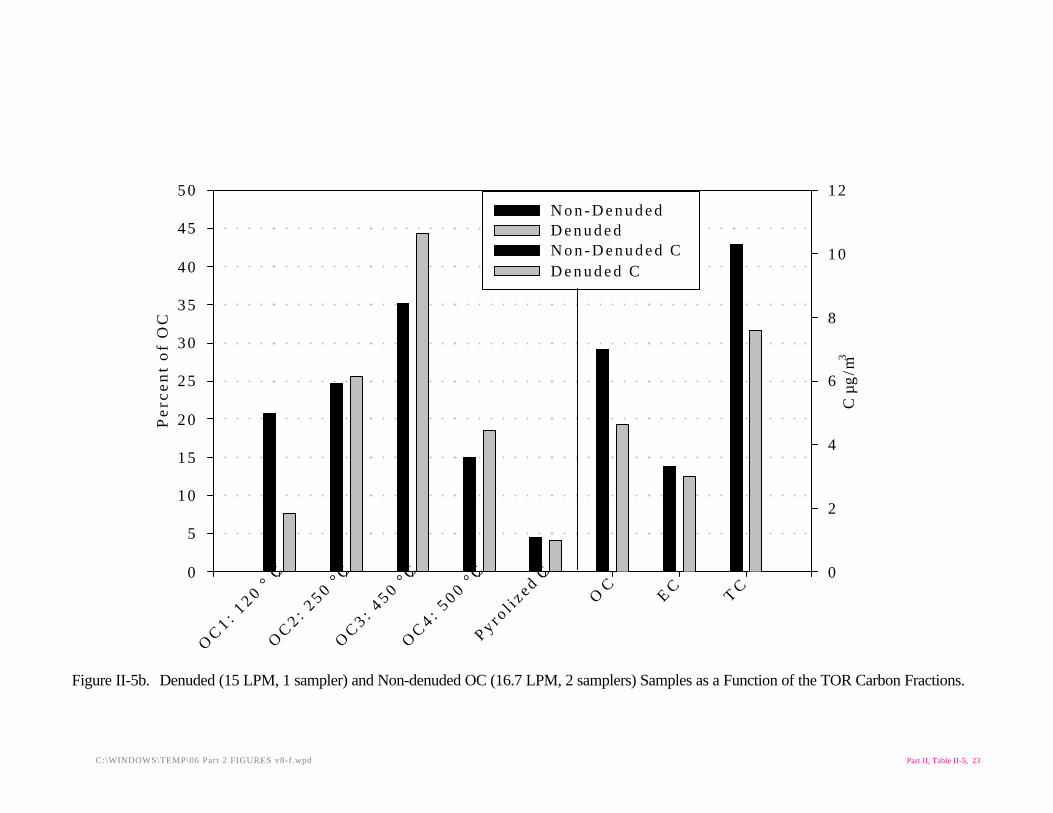
Results from the ANOVA on Particle Nitrate Data . . . . . . . . . . . . . . . . . . . . . Part II, Page 23Aerosol Nitrate . . . . . . . . . . . . . . . . . . . . . . . . . . . . . . . . . . . . . . . . . . . . . . . Part II, Page 24Organic and Elemental Carbon . . . . . . . . . . . . . . . . . . . . . . . . . . . . . . . . . . . . Part II, Page 25

Part I, Page x

Denuded vs Non-Denuded Organic Carbon Results . . . . . . . . . . . . . . Part II, Page 25Comparison between TOR and TOT for OC and EC in PM2.5 . . . . . . Part II, Page 26

Loss of Nitrate During Vacuum XRF Analysis . . . . . . . . . . . . . . . . . . . . . . . . Part II, Page 28

Field Experience with the Speciation Samplers . . . . . . . . . . . . . . . . . . . . . . . . . . . Part II, Page 28Andersen RAAS . . . . . . . . . . . . . . . . . . . . . . . . . . . . . . . . . . . . . . . . . . . . . . Part II, Page 29Met One SASS . . . . . . . . . . . . . . . . . . . . . . . . . . . . . . . . . . . . . . . . . . . . . . . Part II, Page 30URG MASS . . . . . . . . . . . . . . . . . . . . . . . . . . . . . . . . . . . . . . . . . . . . . . . . . Part II, Page 30IMPROVE . . . . . . . . . . . . . . . . . . . . . . . . . . . . . . . . . . . . . . . . . . . . . . . . . . Part II, Page 30VAPS . . . . . . . . . . . . . . . . . . . . . . . . . . . . . . . . . . . . . . . . . . . . . . . . . . . . . . Part II, Page 30FRM . . . . . . . . . . . . . . . . . . . . . . . . . . . . . . . . . . . . . . . . . . . . . . . . . . . . . . . Part II, Page 31

Sampler Costs and Related Spare Parts . . . . . . . . . . . . . . . . . . . . . . . . . . . . . . . . Part II, Page 31

DISCUSSION . . . . . . . . . . . . . . . . . . . . . . . . . . . . . . . . . . . . . . . . . . . . . . . . . . . . . Part II, Page 32

Expectations . . . . . . . . . . . . . . . . . . . . . . . . . . . . . . . . . . . . . . . . . . . . . . . . . . . . . . Part II, Page 32

Major Questions Addressed . . . . . . . . . . . . . . . . . . . . . . . . . . . . . . . . . . . . . . . . . . Part II, Page 32Q1. How well do PM2.5 mass and the chemical components

of mass agree between the FRM and the chemical speciation samplers tested in this study? . . . . . . . . . . . . . . . . . . . . . . . . . . . . . . . Part II, Page 33

Q2. How well can the FRM mass be reconstructed by summing the chemical components measured by the speciation samplers. . . . . . Part II, Page 34Specific Hypotheses Related to Questions Q1 and Q2 . . . . . . . . . . . Part II, Page 35

Denuded vs Non-Denuded Organic Carbon Results . . . . . . . . Part II, Page 38Q3. How well do the measured concentrations from the

various speciation samplers agree? . . . . . . . . . . . . . . . . . . . . . . . . . . . Part II, Page 39Q4. What are the causes of the differences among the speciation

samplers for measured concentrations of mass and the components of mass if they exist. . . . . . . . . . . . . . . . . . . . . . . . . . . . . Part II, Page 39Specific Hypotheses Related to Questions Q3 and Q4 . . . . . . . . . . . Part II, Page 39

SUMMARY AND CONCLUSIONS . . . . . . . . . . . . . . . . . . . . . . . . . . . . . . . . . . . Part II, Page 44Site Characteristics . . . . . . . . . . . . . . . . . . . . . . . . . . . . . . . . . . . . . . . . . . . Part II, Page 44Operations . . . . . . . . . . . . . . . . . . . . . . . . . . . . . . . . . . . . . . . . . . . . . . . . . . Part II, Page 44Measurement Performance . . . . . . . . . . . . . . . . . . . . . . . . . . . . . . . . . . . . Part II, Page 44Implications . . . . . . . . . . . . . . . . . . . . . . . . . . . . . . . . . . . . . . . . . . . . . . . . . Part II, Page 45

Nitrate . . . . . . . . . . . . . . . . . . . . . . . . . . . . . . . . . . . . . . . . . . . . . . . . Part II, Page 45Carbon . . . . . . . . . . . . . . . . . . . . . . . . . . . . . . . . . . . . . . . . . . . . . . . Part II, Page 46

REFERENCES . . . . . . . . . . . . . . . . . . . . . . . . . . . . . . . . . . . . . . . . . . . . . . . . . . . . Part II, Page 47

Part I, Page xi

Tables – Part I . . . . . . . . . . . . . . . . . . . . . . . . . . . . . . . . . . . . . . . . . . . . . . . . Part II Tables, Page 1

Figures – Part I . . . . . . . . . . . . . . . . . . . . . . . . . . . . . . . . . . . . . . . . . . . . . . Part II Figures, Page 1

VOLUME II. APPENDICES

Part I, Page xii

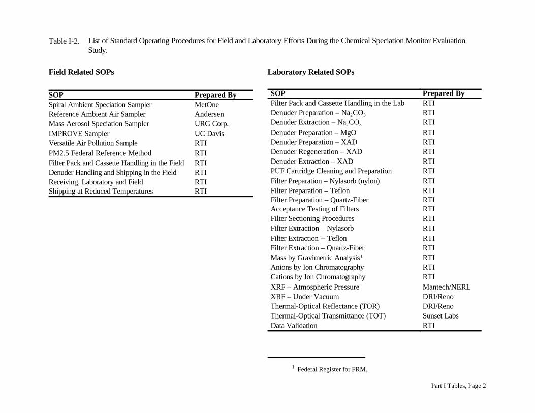
List of Tables – Parts I and IIPart ITable I-1. Analyte Listing for Speciation Sampler IntercomparisonTable I-2. List of Standard Operating Procedures for Field and Laboratory Efforts During the

Chemical Speciation Monitor Evaluation Study.Table I-3. Experimental Design Including Filter and Denuder Preparation.Table I-4. Measurements Made at Rubidoux, CA in Conjunction with the Chemical Speciation

Sampler Evaluation Study.Table I-5. Measurements Made at Phoenix, AZ in Conjunction with the Chemical Speciation

Sampler Evaluation Study.Table I-6. Overall Planned Study Schedule.Table I-7. Field Operations Sampling Schedule.

Part IITable II-1. Summary of Flow Audit Results.Table II-2a. Limits of Detection in ng m-3.Table II-2b. Average Field Blank Data for All Species and Samplers Averaged Across All Sites In

Atmospheric Concentrations.Table II-2c. Precision (as % CV) Achieved by FRM and Speciation Samplers Based on Results

from the Collocated Samplers at Rubidoux.Table II-3. Valid Data Capture in Percent by Sampler and Major Species.Table II-4. Summary of Problems Encountered In the Field During Operations of Sampler

Evaluated in this Study.Table II-5. Species Concentration Data for the FRM at Each Location of the 4-City Study.Table II-6. Estimated PM2.5 Mass Balance of Species versus Measured PM2.5 Mass (ug/m3) for

the FRM at Each Site.Table II-7. Average Volatilized Nitrate (NO3V) in ug/m3 Observed for Each Sampler at Each

City.Table II-8a. Mean Analyte Concentrations for Each Sampler at All Sites.Table II-8b. Ratio of Speciation Sampler to FRM for Chemical Components by Site.Table II-9. Regression Statistics of FRM (x-axis) versus Speciation Samplers (y-axis) for All Sites,

Samplers, and Major Species.Table II-10. Results from the Paired t-Tests Between the Speciation Samplers and FRM Samplers

for Each Analyte/Site.Table II-11. Results from the ANOVA for Examining Equivalency Among the Samplers for

Particulate Nitrate.Table II-12a. Nitrate Concentrations (ug/m3) Measured on Teflon (T) or Quartz-Fiber (Q) Filters by

Sampler Type Averaged Over the Study Period.Table II-12b. Total Particle Nitrate Concentrations (ug/m3) Measured by Each Sampler Averaged

Over the Study Period.

Part I, Page xiii

Table II-12c. Volatilized Nitrate Concentrations (ug/m3) Measured by Each Sampler Averaged Overthe Study Period.

Table II-12d. Sulfate Concentrations (ug/m3) Measured on Teflon (T) or Quartz-Fiber (Q) FiltersAveraged Over the Study Period.

Table II-13a. Nitrate Concentrations (ug/m3) Measured on Teflon (T) or Quartz-Fiber (Q) FiltersAveraged Over the Study Period.

Table II-13b. Total Particle Nitrate Concentrations (ug/m3) Measured by Different Denuder-FilterPack Methods Averaged Over the Study Period.

Table II-13c. Volatilized Nitrate Concentrations (ug/m3) Measured by Different Denuder-Filter PackMethods Averaged Over the Study Period.

Table II-13d. Sulfate Concentrations (ug/m3) Measured on Teflon and Quartz Filters Averaged Overthe Study Period.

Table II-14. Loss of Nitrate Resulting from Analysis of Teflon Filter by Vacuum XRF.Table II-15. Summary of Site Operators Surveys Regarding Speciation Sampler Setup and

operation.Table II-16. Recommended Spare Parts and Supplies for Use of Chemical Speciation Samplers and

FRM Used in the Chemical Speciation Evaluation Study.

Part I, Page xiv

List of Figures – Parts I and IIPart IFigure I-1a. Schematic of the Andersen RAAS Sampler.Figure I-1b. Picture of the Andersen RAAS Sampler Deployed in the Field at RTP.Figure I-2a. Schematic of the MetOne SASS Sampler.Figure I-2b. Picture of MetOne Sampler Deployed in the Field at RTP. Figure I-3a. Schematic of the URG MASS Sampler.Figure I-3b. Picture of the URG MASS Sampler Deployed in the Field at RTP.Figure I-4a. Schematic of the IMPROVE Sampler.Figure I-4b. Picture of the IMPROVE Sampler Deployed in the Field at RTPFigure I-5a. Schematic of the VAPS Sampler.Figure I-5b. Picture of the VAPS Sampler Deployed in the Field at RTP.Figure I-6a. Schematic of the Federal Reference Method Samplers.Figure I-6b. Picture of FRM Samplers Deployed in the Field at RTP.Figure I-7. Schematic of the SCAQMD Multi-Channel Fine Particulate Sampler.Figure I-8. Top – Samplers on the Platform at Rubidoux, CA. Figure I-9. Sampling Platform at Phoenix, AZ.Figure I-10. Philadelphia Sampling Site. Top – Roof View. Figure I-11. Research Triangle Park Sampling Site.

Part IIFigure II-1. Frequency Distributions, Given as Box and Whisker Plots of PM2.5 Species at Each of

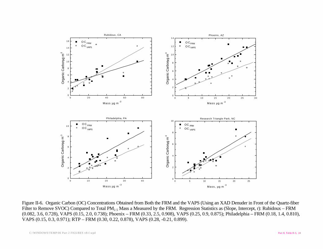
the Four Cities StudiesFigure II-2. Chemical Mass Balance of PM2.5 at Each City.Figure II-3. Time Series Plots.Figure II-4. Regression Analysis Plots.Figure II-5. Denuded and Non-Denuded OC Samples as a Function of the TOR Carbon Fractions.Figure II-6. Organic Carbon concentrations from FRM and VAPS versus Total FRM PM2.5 Mass.Figure II-7. Organic and Elemental Carbon as a function of Face Velocity. Figure II-8. Loss of Aerosol Nitrate from Teflon filters Due to Vacuum XRF Analysis

Part I, Page xv

Volume II List of Appendices – Parts I and II

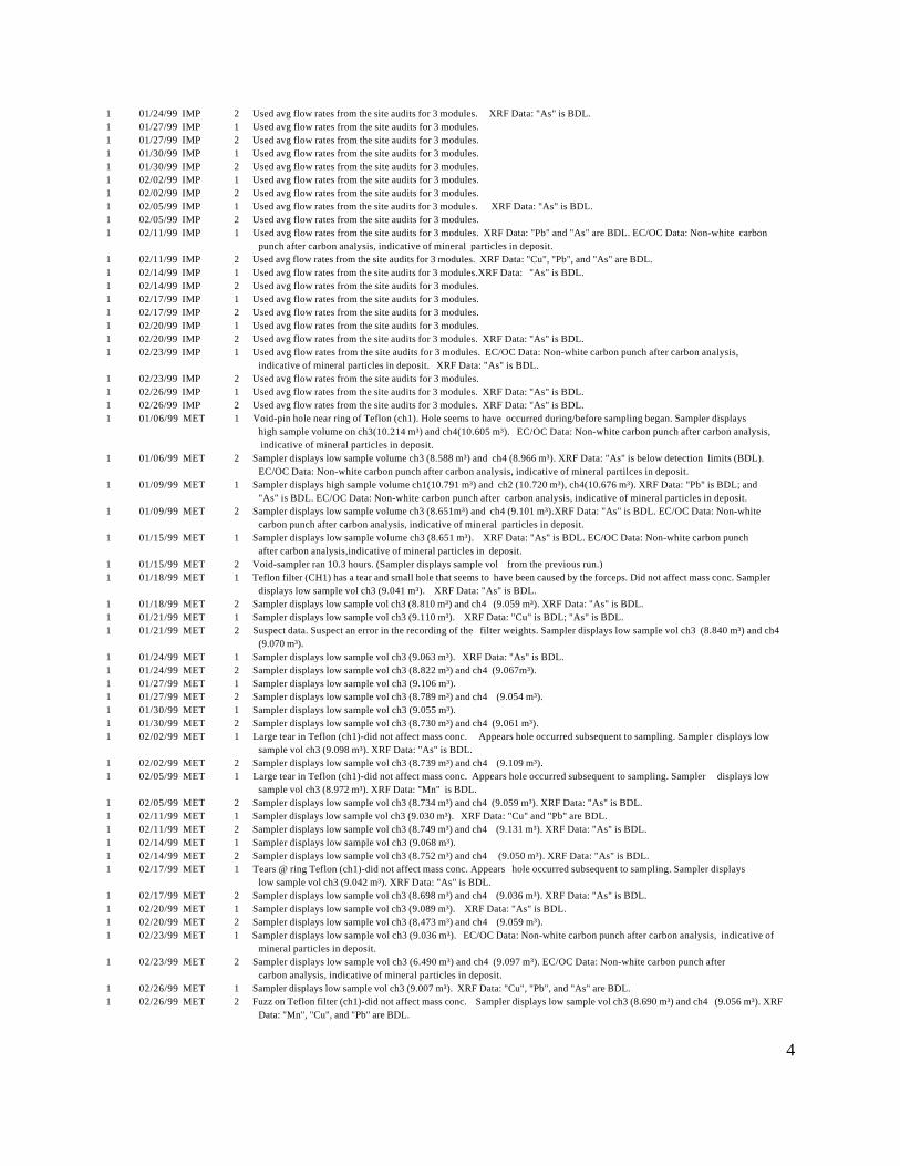
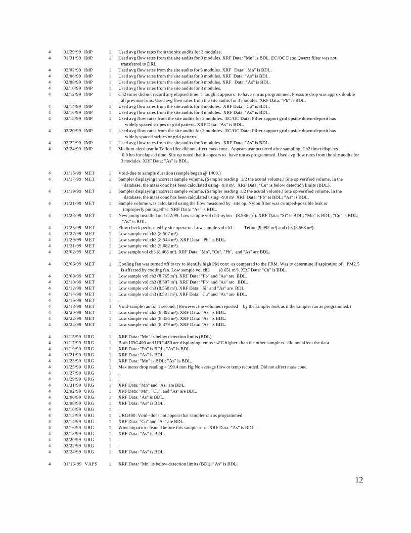
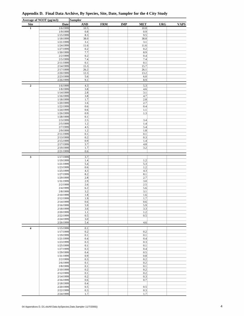
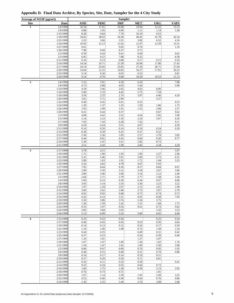
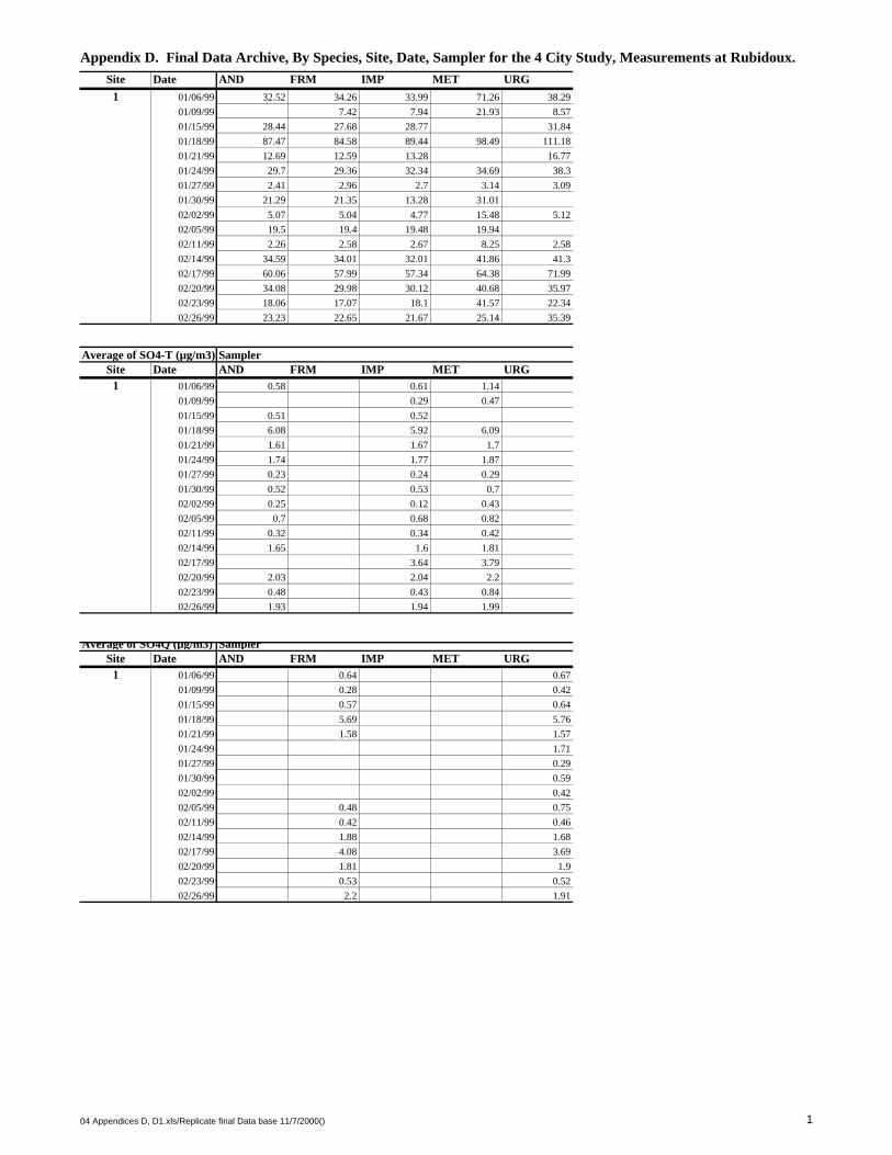
Appendix A: Sample Analysis Methods for Chemical SpeciationAppendix B. Standard Operating ProceduresAppendix C. Summary of Comments from Field and Laboratory Analysis LogbooksAppendix D: Final Data Archive, By Species, Site, Date, and Sampler for the 4-City StudyAppendix D1: Final Data Archive, By Species, Site, Date, and Sampler for Replicate No.2

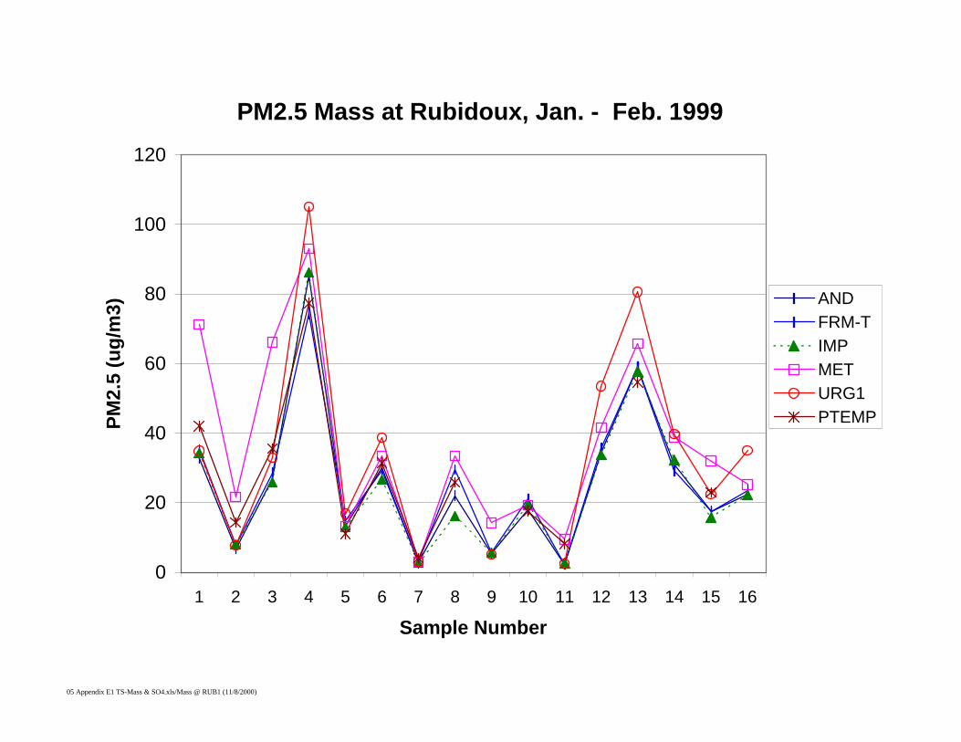
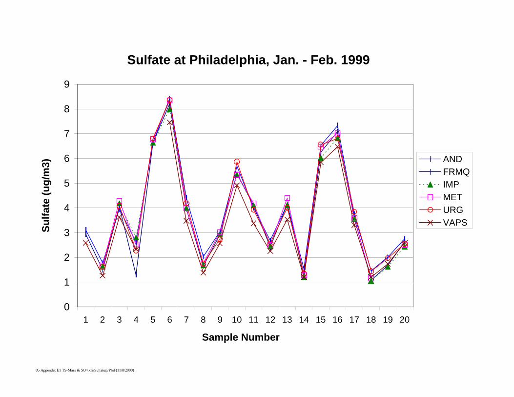
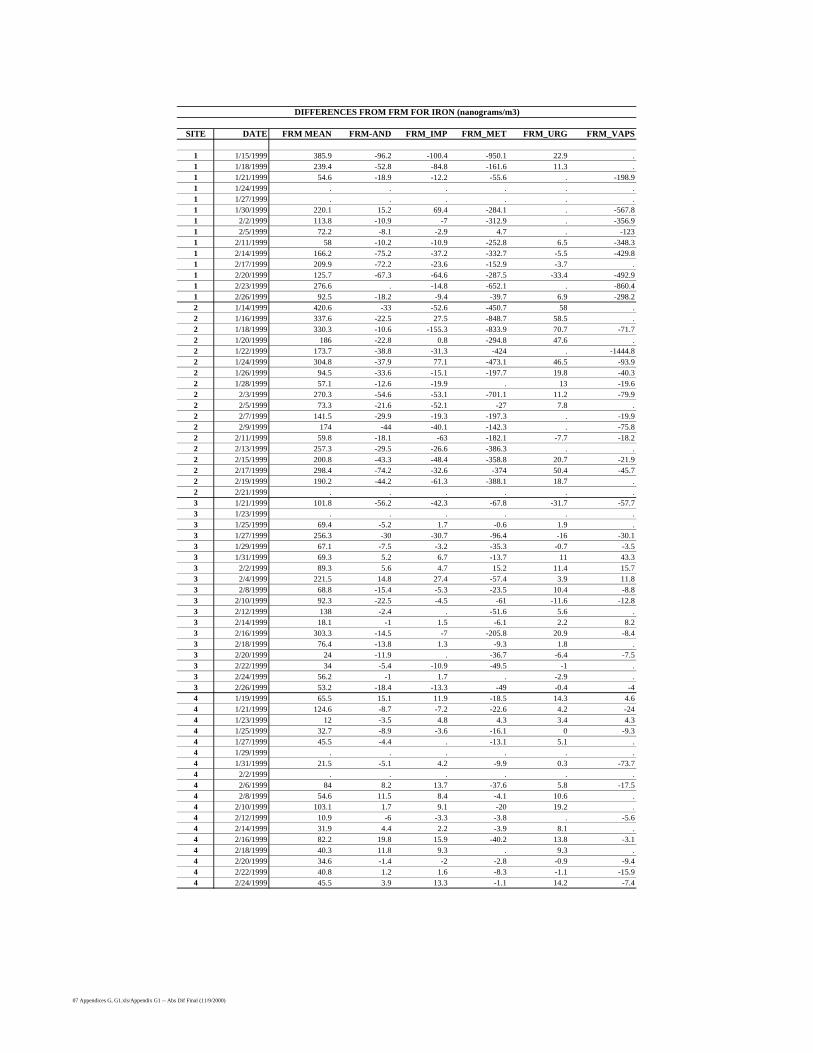
Measurements at RubidouxAppendix E: Time Series Plots for All Species Measured in the 4-City StudyAppendix F: Regression Analysis Plots for All Species Measured in the 4-City StudyAppendix G: Absolute Differences Between the FRM, (Reference Sampler), and the Speciation

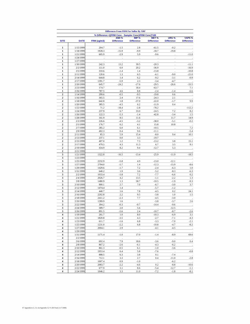
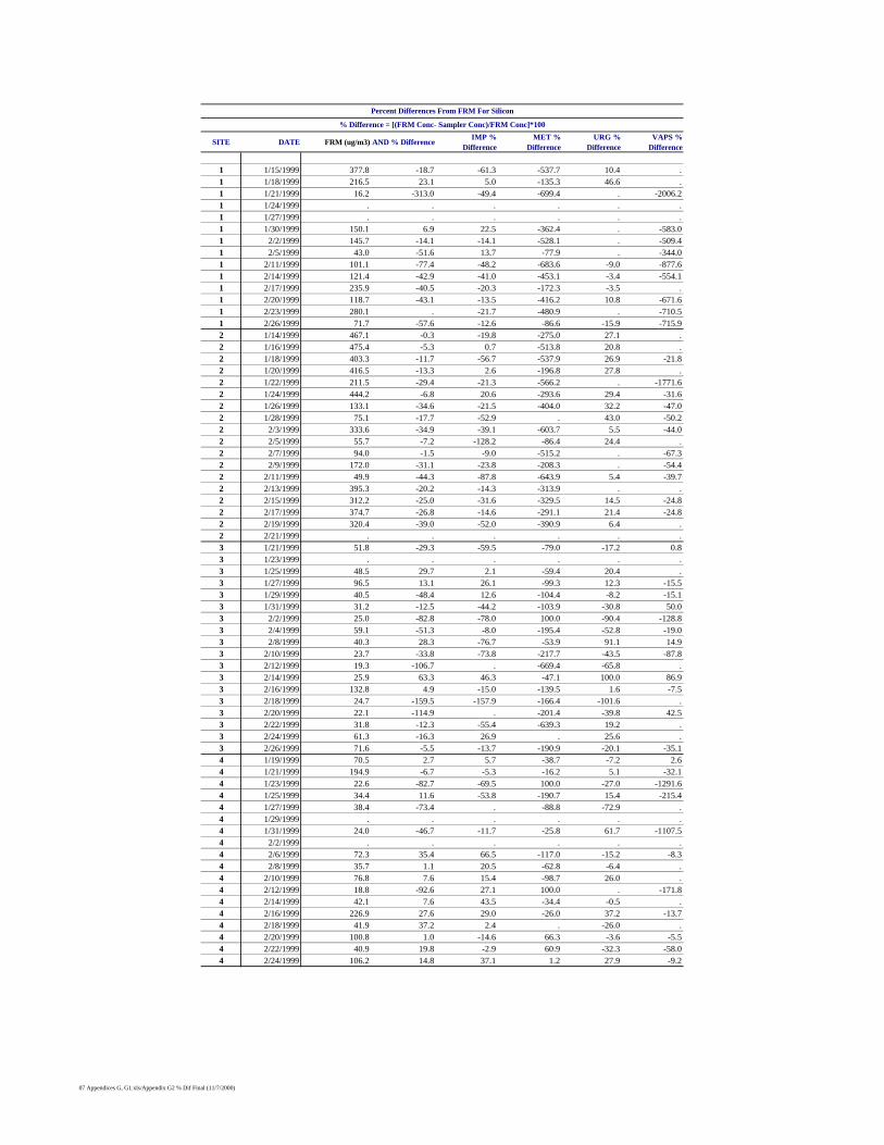
Samplers by Site and By Sampling PeriodAppendix G1: Percent Differences Between the FRM, (Reference Sampler), and the Speciation

Samplers by Site and By Sampling PeriodAppendix H: Field Evaluation of a Spiral and Cyclonic PM2.5 Size Selective Separator for the

MetOne Ambient Chemical Speciation Sampler-SASSAppendix I: Evaluation of PM2.5 Size Selectors Used in Speciation Samplers (Peters et al. 2000)Appendix J: Comparison of Particulate Organic and Elemental Carbon Measurements Made with the

IMPROVE and NIOSH Method 5040 Protocols

Part I, Page 1

Part I

Introduction and Experimental Design

Part I, Page 2

INTRODUCTION

On July 18, 1997, the U.S. EPA promulgated a new NAAQS for particulate matter (PM) in 40 CFRParts 50, 53, and 58, Federal Register (EPA 1997a; EPA 1997b). In addition to slightly revising theprevious PM10 standard, EPA added a new standard for fine particles less than 2.5 µm in aerodynamicdiameter, known as PM2.5. To develop meaningful relationships between PM2.5 levels at receptors andsource emissions and for better understanding the causes of high PM2.5 concentrations, in particularsecondary components formed in the atmosphere through chemical reactions and condensation, it isnecessary not only to sample for PM2.5 mass, the NAAQS indicator, but also for the chemicalcomponents of PM2.5. A sampling program of this type has been initiated by EPA (EPA 1999Guidance Document) that will consist of up to 300 sites at which the major chemical components ofPM2.5 will be measured in the collected aerosol. Since information from this network will be used forthe identification of sources contributing to high PM2.5 mass concentrations, development and evaluationof control strategies, measurement of trends, and support of health studies, it is important that there benational consistency in the species concentrations measured by the PM2.5 speciation network. Inparticular, 54 of these PM2.5 chemical speciation sites will become part of the National Air SamplingStations (NAMS) network and will provide nationally consistent data for assessment of trends (EPA1997b).

Development of chemical speciation samplers for the National PM2.5 Sampler Procurement Contract(National Sampler Contract) was based on performance, rather than design criteria. This has allowedinnovation in the development of these samplers and has resulted in the development of three slightlydifferent samplers for meeting the specified performance criteria. Also as a result of this approach, aguidance document on chemical speciation of particulate matter has been prepared by EPA (EPA,1999) and reviewed by an external peer-review panel (Speciation Expert Panel; Koutrakis, 1998). Intheir first review, the expert panel recommended an intercomparison among the chemical speciationsamplers. The intercomparison also should include other historically accepted samplers (e.g., theimproved IMPROVE sampler, the Harvard Sampler, or some other sampler) and the PM2.5 FederalReference Method (FRM). The chemical species to be determined should include those recommendedby the expert panel (Koutrakis, 1998) and as specified in the guidance document for chemical speciation(EPA, 1999). The program plan for EPA’s Chemical Speciation Sampler Evaluation Study (Solomonet al. 1998) outlines the approach and details the implementation of the intercomparison study toperform an initial evaluation of the chemical speciation samplers developed in response to the NationalSampler Contract and several other samplers developed earlier and independently of the EPA nationalprogram.

About this ReportThis draft final report provides results from EPA’s Chemical Speciation Sampler Evaluation Study (4City Study). The data presented in this report have been validated through Level 2b, that is, the datahave undergone multi-variate statistical analyzes for consistency and known physical relationships andinterpretive data analysis (NARSTO 1999). Part I of this report outlines the study, provides a

Part I, Page 3

summary of the samplers and the chemical analysis methods, and outlines the major questions andhypotheses to be addressed by this evaluation. Part II presents the results. First, quality assuranceresults are summarized, including operations and maintenance and systems and performance audit resultsfollowed by a summary of the chemical characteristics observed at each location. Next, results arepresented from the statistical evaluations of the data, including time series analysis, regression analysis,difference analysis, T-test, and Analysis of Variance. In the Discussion Section, each hypothesis notedin the program plan, and Part I of this document is addressed to the extent possible and within thelimitations of the study design. Lastly, an overall summary is provided.

Study ObjectivesThe objective of this sampler intercomparison study is to determine if there are differences among thethree PM2.5 chemical speciation samplers developed in response to the National Sampler Contract andhow these samplers compare relative to other historical samplers, and to the FRM. While the FRM isthe “gold” standard for mass, there are no such standards for the chemical components of PM2.5. Thus,this intercomparison only establishes the relative equivalence of the samplers to each other on a speciesby species basis. For semi-volatile species (those in dynamic equilibrium between the gas and particlephases; e.g., for ammonium nitrate), the FRM using Teflon filters provides only a lower limit on theexpected mass loading, since there is potential for loss of nitrate and semi-volatile organic species(SVOC) from the inert Teflon filters. For stable species, the FRM should provide an accurate estimateof the mass loading for those species. Chemical speciation samplers used historically [e.g., the VersatileAir Pollution Sampler (VAPS) developed under an EPA contract, the Caltech gray box sampler(Solomon et al., 1989), or the South Coast Air Quality Management District’s PM10 TechnicalEnhancement Program (PTEP) sampler (SCAQMD, 1996) should provide a less biased value for semi-volatile species (i.e., ammonium nitrate) and provide an additional set of samples for comparison;however, they still can only be compared on equivalent bases.

Overview of the IntercomparisonCollecting atmospheric particulate matter using the FRM with Teflon filters can result in negativesampling artifacts associated with the collected sample. Potential artifacts include the loss of volatilespecies, such as ammonium nitrate (Solomon et al., 1988, Hering et al., 1988; Hering and Cass 1999)and semi-volatile organic compounds (Cui et al., 1997; Eatough et al. 1995). Use of other filter mediaalso may result in negative or positive sampling artifacts. The magnitude of these potential artifactsdepends upon the atmospheric concentration of the species being affected, the temperature, relativehumidity, and other variables (e.g., for nitrate, Russell and Cass, 1986; Hering and Cass, 1999). Thechemical speciation samplers developed for National Sampler Contract have been designed to minimizethese potential biases or artifacts by the use of diffusion denuders to remove gas phase species andreactive substrates to collect species that may volatilize during or after sampling from the inert filter (e.g.,Teflon membrane) where the aerosol is collected. Therefore, to evaluate the performance of thesechemical speciation samplers they must be able to properly determine the chemical components ofPM2.5 under a variety of atmospheric conditions, each of which will place different stresses on the

Part I, Page 4

performance of the sampler designs. For this study, this was accomplished by sampling at differentlocations throughout the country, since the composition of the atmospheric aerosol is not uniform acrossthe country (Pace, 1998). For example, some areas have high nitrate and low sulfate levels (LosAngeles, CA: Solomon et al., 1989), while others (e.g., the eastern part of the United States) haverelatively high sulfate and low nitrate levels (Hidy 1994, Pace, 1998). Still, other areas are dominatedby aerosol rich in organic compounds derived from automobile exhaust (Los Angeles, CA: Schauer,1996) , by organic aerosol derived from wood smoke combustion (Fresno, CA: Schauer, 1998), orfrom by organic aerosol derived from natural biogenic emissions (e.g., Southeast US). Some areas ofthe country are highly influenced by crustal material (e.g., Southwest US: Pace 1998; Eldred et al. 1998a). In actuality, several of these conditions exist simultaneously, with one or two components beinghigher then the others (Pace 1998; Eldred, 1998a, Solomon et al. 1989).

A variety of atmospheric chemical conditions also may be observed at one location during different seasons(Pace, 1998). For example, sulfate is likely highest in the east during the summer when photochemistry ishigh, while nitrate is highest in the west in the winter when cool temperatures drive the ammonium nitrateequilibrium with nitric acid and ammonia to the aerosol phase. However, due to the need to have resultsby mid-1999, the study was conducted over about an eight week period at four different locations to obtainas wide a difference in chemical atmospheres as possible. These constraints, however, resulted inlimitations, and follow-on studies will have to occur to fully test the equivalency of these samplers under awider variety of conditions. For example, by sampling in the winter in the east, we missed the highest sulfateconcentrations which occur in the summer (Hidy, 1994), we did not sampling at a site with high woodsmoke emissions, we sampled in Phoenix for crustal material in the winter when the highest crustalconcentrations are likely to be observed in the hot dry summers, and the samplers did not experienceextreme cold temperatures as might be expected in the northern mid-west or hot humid summers asexperienced during the summer in the east.

Due to time and resource limitations, sampler evaluation is being conducted in four phases. Phase I iscentered on sampling in areas with the following atmospheric conditions: high sulfate and low nitrate(east coast US), high nitrate and low sulfate (California), and high crustal material (Phoenix, AZ). Thefourth site is located near ORD headquarters in Research Triangle Park to allow for a more thoroughevaluation of the samplers and their in-field operational performance. Phase II is taking place in Seattle,WA from March-July, 1999 and is evaluating the efficiency and capacity of organic diffusion denudersand reactive back-up sorbents, including ones not currently planned for the chemical speciationsamplers. Phase III is an extensive comparison of the same speciation samplers used in the 4 CityStudy, as well as several others that have been developed at universities. Comparisons in Phase III alsowill be made to a number of species specific continuous methods for the major components of PM2.5. Phase IV is a ten city study where the sites will have at least 2 speciation samplers and be operated bythe States.

The time schedule for Phase I of the study dictated that we sample more frequently than every 6th day,as the results are needed by OAQPS by mid-June, 1999 for input into the decision process for choosing

Part I, Page 5

chemical speciation samplers for the National Air Monitoring Stations (NAMS) TRENDS network. Therefore, samples were collected every-other-day. The statistical design required a minimum of 10-15samples. To ensure that a sufficient number of samples were collected to meet that objective, 20sampling periods were attempted. Samples were analyzed for the major chemical components usingstandard analytical techniques as described below and recommended by the expert panel that reviewedthe guidance document (Koutrakis, 1998). Data analysis provided a robust test of the equivalency ofthe samplers studied and, within the limitations of the study, reasons for differences among the methodstested.

Phase II involves sampling in Seattle, WA with a focus on understanding the collection of organicmaterial (aerosol OC and semi-volatile organic compounds) under wood smoke conditions in a mannerthat will minimize negative and positive sampling artifacts for organic species. These systems include adenuder to remove semi-volatile organic compounds that are in the gas phase and may be collected bythe downstream quartz fiber filter, followed by a reactive sorbents (denuder, PUF, or impregnatedfilter). The evaluation includes determining capacity, efficiency, and comparability of two denudersystems and an evaluation of the sorbents located behind the quartz fiber filter. The first system usesXAD-4 coated onto annular denuders as was proposed for use in two of the chemical speciationsamplers procured through the National Sampler Contract (University Research Glassware andAndersen Instruments). The second system uses a multi-channel parallel plate denuder composed ofcarbon impregnated filters (CIF) (Eatough et al., 1993). Both denuders are followed by quartz fiberfilters which are then followed either by second XAD-4 coated denuder, an CIF filter, an XAD-4impregnated Whatman filter, PUF cartridge, or an XAD-4-sorbent bed. XAD-4, PUF cartridges, andquartz fiber filters can be extracted and individual species can be determined to obtain a mass balancebetween the SVOC, aerosol organic species collected on the quartz fiber filter, and the SVOCvolatilized from the quartz fiber filter and collected on the reactive back-up medium, on a species-by-species basis. The CIF filter can be analyzed for organic carbon using thermal desorption.

Phase III will involve sampling in Atlanta, GA where biogenic VOC emissions are known to be high inthe summer (Chameides et al. 1988). The Atlanta intercomparison is an integral part of the EPASupersites Program (EPA 1998). The same set of chemical speciation monitors will be operated inAtlanta as were operated in the 4 City Study. In addition, several other speciation samplers areincluded in the intercomparison along with the potential for comparisons to a number of species specificcontinuous methods for sulfate, nitrate, ammonium, trace elements (Na - Pb), organic carbon, andelemental carbon. Details of the Atlanta study are described in Hering (1999).

Phase IV, the Ten City Study is still in planning. It is anticipated, that each site will have at least twodifferent chemical speciation samplers, operate on a 1 in 3 day schedule from about October 1999through March 2000, and have chemical analysis performed in the national laboratories established tosupport the chemical speciation sampling network. The goal of this study is to evaluate the samplers

Part I, Page 6

under more severe extremes of temperature, as well as higher crustal material and wood smokeloadings.

Study DesignThe design of this program is constrained by limitations in the time frame allowed for the experiment andin resources available to complete the program (e.g., number of samplers, personnel, and funding). However, the statistical design was prepared understanding these limitations and the design chosenprovides a robust evaluation of the samplers relative to each other, to several samplers used historicallyto obtain similar data, and to the FRM. The overall design is detailed below.

Statistical DesignThe primary objective of this study is to determine if there are differences in the measuredconcentrations of the chemical components of PM2.5 mass as determined by the three PM2.5 chemicalspeciation samplers available on the National Sampler Contract . Comparisons also will be made totwo historical samplers and to the FRM using these samplers as a relative reference. A secondaryobjective of this study is to evaluate the operational performance or practicality of the samplers in thefield, that is, reliability, ruggedness, ease of use, and maintenance requirements.

There are three major scientific hypotheses to be addressed by this intercomparison study.

< One is associated with reconstructing the FRM mass.

< The second is associated with comparing the measured chemical concentrations amongthe various speciation samplers, which consists of two parts:

! The first part is associated with examining differences among the samplers,without regard to why there are differences, if they exist.

! The second part examines why there are differences, if they exist. Some areexpected due to the slightly different methods employed.

< A third set of hypotheses is given dealing with the potential affect of different analyticalmethods on measured concentrations of the chemical components of PM2.5. Theseinclude the effect of vacuum X-ray fluorescence (XRF) or atmospheric pressure XRFon nitrate concentrations measured on Teflon filters and the effect of thermal opticalreflectance (TOR) vs. thermal optical transmittance (TOT) on the determination oforganic and elemental carbon (OC/EC) concentrations from pre-baked quartz fiberfilters.

The first two hypotheses are predicated on the assumption that the cutpoints (50% collection efficiency)for the samplers used in this study have essentially the slope and 50% cutpoint. This is a required

Part I, Page 7

assumption to address these hypotheses. Also, it is important to establish the precision of theinstruments, which was obtained by collocating samples at one site (Rubidoux, CA). While thisprovides only a limited assessment of the precision, it provides a first cut estimate of the precision for thestatistical analyses performed to understand the data. If for example, the precision is estimated at 50%,then determining differences among samplers is not as informative as if the precision were 10-15%. Asa benchmark, the coefficient of variation for the differences in concentrations from collocated FRMinstruments is required to be less than 10%, according to 40 CFR Part 58, Appendix A. Depending onthe species, we anticipate a range of precision from less than 10% to about 30%.

A detailed list of hypotheses is given in the Statistical Analysis section.

Part I, Page 8

EXPERIMENTAL

Sampler Types and RationaleChemical speciation samplers have been developed and built by three different manufacturers under theNational Sampler Contract procurement. The need for PM2.5 chemical speciation monitoring isdescribed under 40 CFR, Parts 53 and 58 (EPA 1997). The three samplers are the Reference AmbientAir Sampler (RAAS) developed by Andersen Instruments Incorporated (Andersen), Mass AerosolSpeciation Sampler (MASS) developed by University Research Glassware Corporation (URG), andSpiral Ambient Speciation Sampler (SASS) developed by Met One Instruments (MetOne). Theexternal peer-review committee (Koutrakis, 1998) recommended comparison of these samplers underfield conditions in different areas of the country and different seasons. They also recommendedcomparison to samplers used previously that have been accepted historically as providing data of knownuncertainty, and to the FRM.

Historical methods included in this study were the National Park Services’ IMPROVE (InteragencyMonitoring of Protected Visual Environments) sampler modified to include 47 mm filters as suggested bythe expert review panel (Koutrakis, 1998), the Versatile Air Pollution Sampler (VAPS)(URGCorporation; four available), and the PTEP sampler (SCAQMD, 1996) operated by the South CoastAir Quality Management District (SCAQMD) at their Rubidoux, CA site. These samplers are wellcharacterized for collecting relatively unbiased samples suitable for chemical analysis of major PMcomposition.

Two FRM samplers were operated at each site to allow for chemical characterization of the collectedsample similar to that being obtained by the chemical speciation samplers. One FRM collects aerosolsamples on Teflon filters for mass and trace elements (Na - Pb), while the other FRM used quartz-fiberfilters for determination of ions (SO4

=, NO3-, and NH4

+), OC, and EC.

The FRM should provide a suitable reference for stable species, such as many of the trace metals andsulfate. The historical samplers should provide a reference for labile compounds (nitrate ion and semi-volatile organic compounds [SVOC]) as they used diffusion denuders and reactive backup filters, similarto the chemical speciation samplers, thus minimizing the potential gain or loss of these species whenusing only Teflon or quartz fiber filters. The IMPROVE sampler should provide nearly artifact free datafor nitrate, while the VAPS should provide nearly artifact free data for nitrate and organic carbon. During Phase I, only the VAPS used a denuder for removing gas-phase semi-volatile organiccompounds (referred to here after as an organic denuder), as there is currently considerable uncertaintyin using organic denuders as well as the desire to leave research oriented approaches to more carefulexamination. Collection of organic carbon using denuders and reactive collection media is addressed inPhase II activities.

Both the VAPS and the IMPROVE samplers have been used and evaluated in numerous studies overthe last decade, and thus, provide a reference to many other databases (Shaibal et al. 1997;

Part I, Page 9

Sommerville et al. 1994; Stevens et al., 1993; Pinto et al. 1998; Mathai et al. 1990; Cahill, 1993). ThePTEP sampler, only operated at Rubidoux, also falls into this category as it has been used for nearly adecade by the South Coast Air Quality Management District (SCAQMD) in southern California(Teffera et al., 1996; SCAQMD, 1996). The PTEP sampler also uses methods similar to the chemicalspeciation samplers.

Sample analysis, which is described in more detail later, included mass by gravimetric analysis, ions(sulfate, nitrate, and ammonium) by ion chromatography (IC), OC/EC by thermal-optical reflectance(TOR), and elemental analysis by energy dispersive X-ray fluorescence (XRF). Mass was alwaysdetermined on Teflon filters following FRM protocol for filter equilibration and weighing. Concentrations of trace elements (Na - Pb), were measured on the same filter used for massdeterminations. Ions are determined from aqueous extracts of either Teflon (wet with 50 µl ethanolbefore extraction), quartz-fiber, or nylon filters. Nylon filters analyzed for only for nitrate were extractedin IC eluent and those analyzed for nitrate, sulfate, and ammonium ions were extracted in water. OCand EC were measured on quartz-fiber filters that have been baked at 600oC for 2 hours to lowerbackground carbon levels below 0.2 µg/cm2 total carbon. Quartz-fiber filters analyzed for ions weresplit to allow for carbon and ions analysis. All other filters were kept whole for analysis.

Sampler Descriptions - The Chemical Speciation SamplersDesign of the three chemical speciation samplers for the National PM2.5 Network can be found in theEPA chemical speciation guidance document (EPA, 1999). The draft guidance document outlines thegeneral design of these samplers as envisioned for the PM2.5 network; although they are not likely thefinal designs to be implemented, as this and future field evaluations of the samplers may result inmodifications to the samplers. Specific designs of the samplers for this intercomparison are given below. In general, each sampler draws air at a specified flow rate through a size selective inlet that removesparticles greater than a specified size with a 50% collection efficiency or cutpoint. For the samplersemployed in this study the cutpoint is 2.5 µm. As recommended by the expert peer-review panel(Koutrakis, 1998), the efficiency of collection (slope and cutpoint) for each sampler should closelyresemble that of the FRM, and that was under the control of the manufacturers. Described below arethe three samplers provided to EPA for the National Sampler Contract procurement by URG, MetOne,and Andersen.

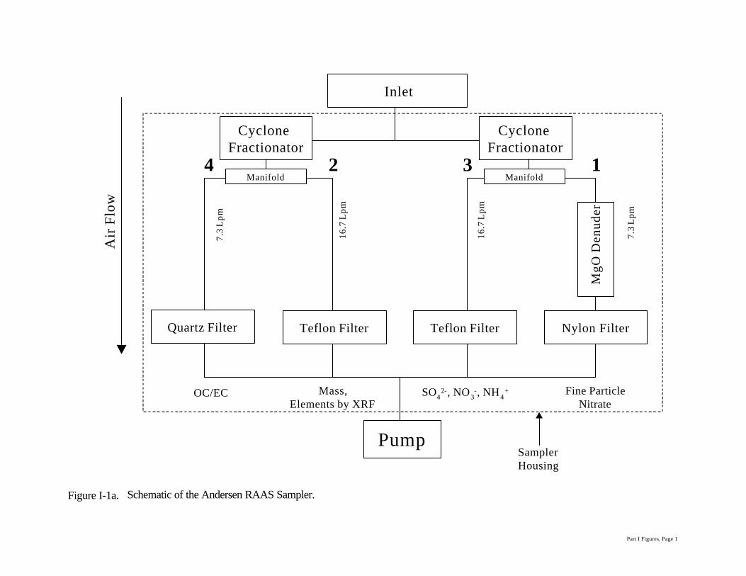
Reference Ambient Air Sampler (RAAS) developed by Andersen InstrumentsA schematic flow diagram of the Andersen RAAS is shown in Figure 1a, with a picture of the samplergiven in Figure 1b. It consists of a size selective inlet followed by two PM2.5 cyclones in parallel, theoutlets of which are connected to separate sampling manifolds. These cyclones are used to removeparticles greater than 2.5 micrometers with a 50% collection efficiency, when operated at 24 Lpm. Theflow is then split in each manifold into 2 channels (maximum of 3) for at total of up to 6 channels. Of thefour channels used in this study, the first channel (labeled 1 in Figure 1a) is used to estimate atmosphericconcentrations of particulate organic and elemental carbon (OC/EC). The flow rate in this channel is

Part I, Page 10

7.3 Lpm. In the second channel (labeled 2 in Figure 1a), particulate matter is collected on a Teflon filterfor analysis of mass and trace elements (Na - Pb) by energy dispersive X-ray fluorescence (XRF). Theflow rate through this channel 2 is 16.7 Lpm. In the third channel (labeled 3 in Figure 1a) particulatematter also is collected on a Teflon filter, which is extracted in water and analyzed for sulfate, nitrate,and ammonium ion concentrations by ion chromatography (IC). The last channel (labeled 4 in Figure1a) is used to obtain a nearly unbiased estimate of fine particle nitrate by removing acidic gases (e.g.,HNO3) from the air stream using a diffusion denuder coated with MgO and collecting aerosol nitrate ona reactive Nylasorb (nylon) backup filter. This assumes the denuder is efficient for HNO3 and otheracidic gases that might be collected on the nylon filter and analyzed as nitrate and that the nylon filterdoes not collect NO2. The filter is extracted in IC eluent and analyzed by IC for nitrate. In all channels,critical orifices control the flow and the flow rates are monitored using electronic mass flow sensors. Allinternal components before the filter holders or denuders are Teflon® coated and no grease or oil is usedin the sampler’s design. The system also monitors continuously relative humidity (RH), barometricpressure (BP), orifice pressure (OP), ambient temperature (T), manifold temperature (MT), metertemperature (MeT) and cabinet temperature (CT). Data can be downloaded through a RS-232C serialport, which also allows for two way remote communication (Andersen, 1999).

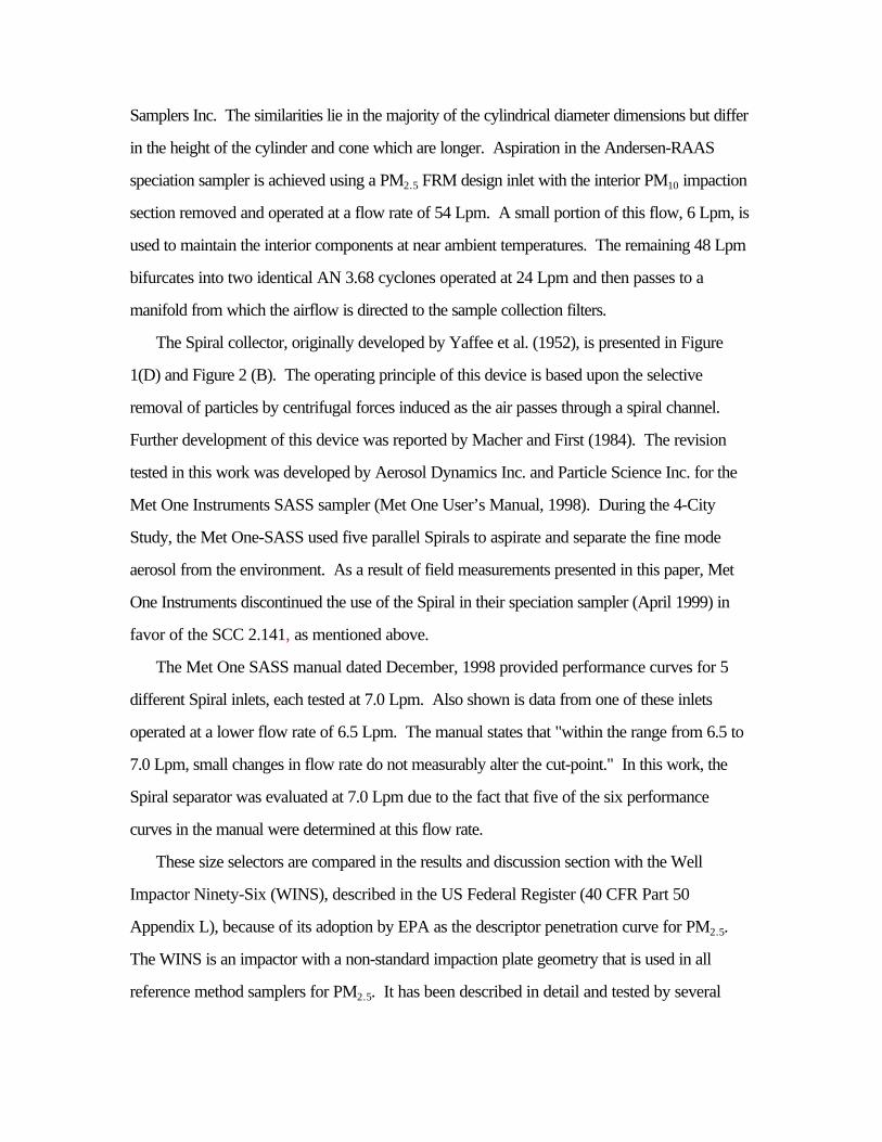
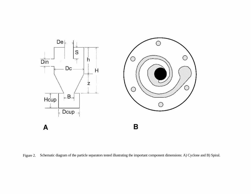
Spiral Ambient Speciation Sampler (SASS) developed by MetOneA schematic flow diagram for the MetOne SASS sampler is presented in Figure 2a, with a picture of thesampler shown in Figure 2b. The SASS has 5 separate channels, operated through a commoncontroller and pump. For the current Four City Study, each channel contained a spiral impactordesigned to give a 2.5 µm cut-point (50% collection efficiency) with a slope and cutpoint similar to theFRM when operated at 6.7 Lpm (MetOne, 1999). {Note, results from this study indicted that underhigh coarse particle loading conditions, the Spiral impactor allowed large particles to penetrate to thefilter. The Spiral is being replaced by a sharp cutpoint cyclone (SCC) developed by BGI, Incorporated. The rest of the design for the SASS sampler is staying essentially the same.} The first channel (labeled1 in Figure 2a) collects particulate matter on a Teflon filter that is analyzed for atmosphericconcentrations of PM2.5 mass and trace elements (Na - Pb). The second channel (labeled 2 in Figure2a) also collects particulate matter on a Teflon filter that is analyzed for sulfate, nitrate, and ammoniumion concentrations. A MgO coated aluminum honeycomb diffusion denuder is located behind the spiralimpactor in the third channel (labeled 3 in Figure 2a). This denuder is used to remove acidic gases (e.g.,HNO3) from the sampled air stream. The MgO denuder is followed by a Nylon filter that is analyzedfor nitrate as described above. As in the RAAS sampler, the denuder/reactive filter pair is used toobtain a nearly unbiased estimate of aerosol nitrate. This assumes the denuder is efficient for HNO3 andother acidic species that might be analyzed as nitrate, and that the nylon filter does not collect NO2. Thefourth channel (labeled 4 in Figure 2a) contains two baked quartz-fiber filters located behind the spiralimpactor. The first quartz-fiber filter is analyzed for OC/EC by thermal-optical reflectance, while thesecond quartz-fiber filter is archived. The fifth channel (labeled 5 in Figure 2a) also contains 2 bakedquartz-fiber filters as a replicate set to channel 4. This set of quartz fiber filters are archived for futureuse. In Phase III (Atlanta), it is anticipated that a elemental carbon honeycomb diffusion denuder willbe available for use in channel 5. This denuder is used to remove semi-volatile organic compounds that

Part I, Page 11

may interfere, as a positive artifact, with the OC measurement. The flow rate through each channel isnominally 6.7 Lpm and is controlled by a critical orifice. The flow rate in this instrument is monitoredusing electronic mass flow sensors.

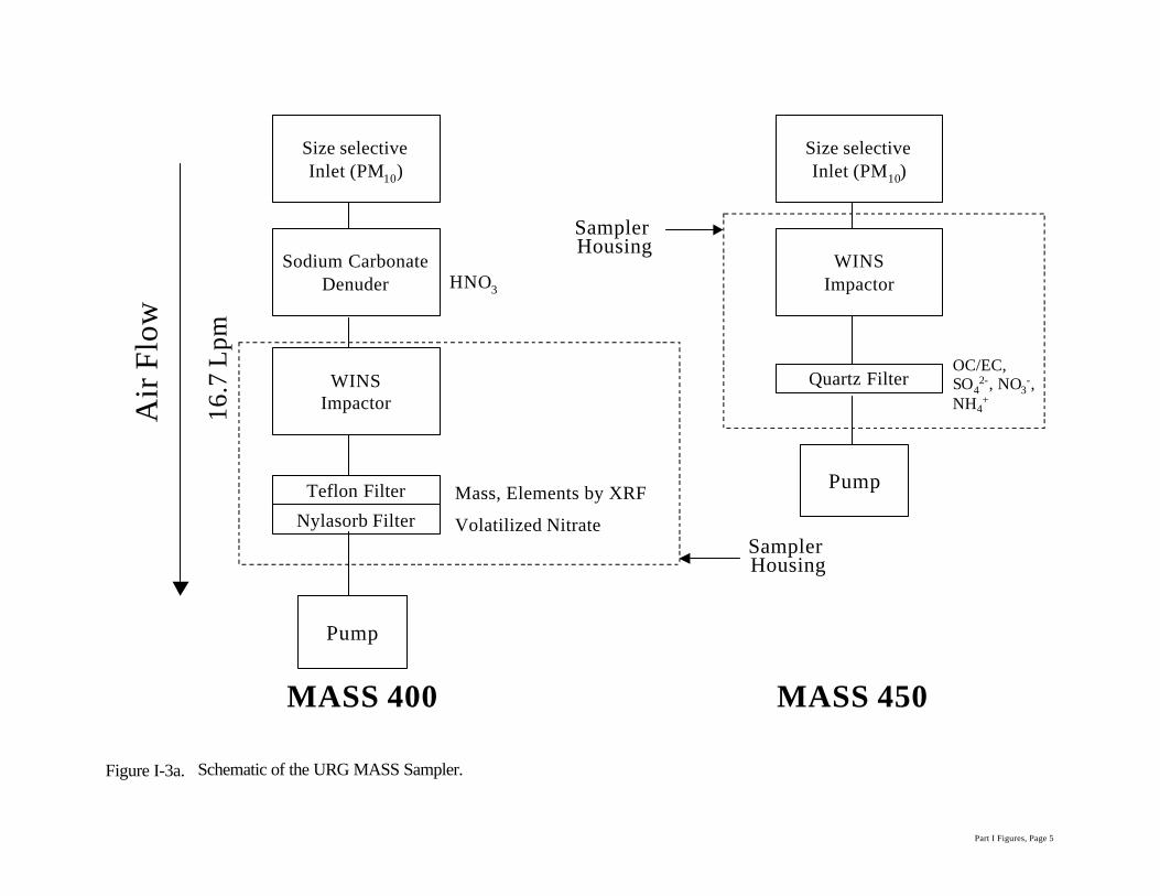
Mass Aerosol Speciation Sampler (MASS) developed by University Research Glassware(URG)The URG MASS sampler is shown in Figure 3a with a picture of this sampler given in Figure 3b. This sampler consists of two modules (URG MASS 400 and MASS 450), each with an FRM PM10sizeselective inlet and a WINS impactor for the collection of PM2.5 aerosol. The MASS 400 is equippedwith a Na2CO3 denuder before the WINS impactor but after the PM10 size selective inlet. This denuderis used to remove acidic gases much like the MgO denuders discussed above. The particles less than2.5 µm are collected on the top filter of a dual filter pack, which is an inert Teflon filter that is analyzedfor PM2.5 mass and trace elements (Na - Pb). The backup nylon filter efficiently collects nitrate thatmay have vaporized from the front Teflon filter during sampling. Nitrate ion is quantified using IC afterextraction from the Teflon and nylon filters as described above for the RAAS sampler. The sum ofnitrate measured on the Teflon and nylon filters provides a nearly bias free estimate of fine particlenitrate. This assumes the denuder is efficient for HNO3 and that the nylon filter does not collect NO2. The MASS 450 contains a single filter pack containing one pre-baked quartz-fiber filter. This filter issplit in half with OC and EC determined from one half and sulfate, nitrate, and ammonium ionsdetermined on the other half. An organic denuder (XAD coated annular denuder) is not used here, butwill be used in Phase III of the study following recommendations from Phase II. The flow rate througheach module is nominally 16.7 Lpm. Flow is monitored using a dry gas meter with a feed back loop tothe controller to adjust for variations in flow rate as particles are collected on the filter.

Sampler Descriptions - Historical SamplersHistorical samplers include the IMPROVE, VAPS, FRM, and PTEP samplers, the latter being operatedonly at Rubidoux as part of a SCAQMD PM chemical characterization study (SCAQMD, 1996).

IMPROVE SamplerDetailed descriptions of the IMPROVE sampler can be found in Eldred et al. (1998b). A schematicdiagram of the IMPROVE is given in Figure 4a with a picture of the sampler given in Figure 4b. Ingeneral, the IMPROVE sampler consists of several modules each of which is dedicated to collecting aseries of related chemical components of the atmospheric aerosol. Each module consists of a sizeselective inlet, a cyclone to provide a PM2.5 size cutpoint based on the specified flow rate, filter mediafor sample collection, a critical orifice that provides the proper flow rate for the desired size cutoff, and avacuum pump to produce the flow. Flow rate is not monitored continuously, but are verified prior toand after each sampling period. The IMPROVE samplers consist of up to four parallel modules, and acommon controller (timer) as described in Eldred et al. (1998). Only three modules are used in thisstudy, as the fourth is typically used to collect PM10. The first module (labeled 1 in Figure 4a) collectsPM2.5 on a Teflon filter, for determining atmospheric concentrations of PM2.5 mass and trace elements(Na - Pb). The second module (labeled 2 in Figure 4a) includes a Na2CO3 denuder before the PM2.5

Part I, Page 12

cyclone to remove acidic gases (e.g., HNO3) followed by the cyclone and a nylon filter. This nylon filteris analyzed for sulfate, nitrate, and ammonium ions. The third module (labeled 3 in Figure 4a) collectsPM on a pre-baked quartz-fiber filter. This filter is analyzed for OC and EC.

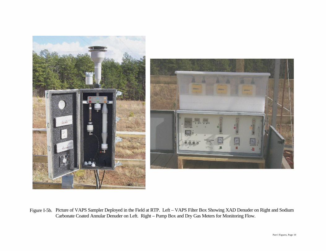
Versatile Air Pollution SamplerThe VAPS sampler is shown in Figure 5a with a picture of the sampler given in Figure 5b. A PM2.5

cutpoint is obtained using a size selective impactor followed by a virtual impactor with a PM2.5 cutpoint. The coarse particles follow the minor flow (3 Lpm) and are collected on a Teflon filter from whichcoarse (PM10-PM2.5) particles mass is obtained. The fine (< PM2.5) particle flow (30 Lpm) is splitevenly between two channels. One channel (labeled 1 in Figure 5a) contains a diffusion denuder coatedwith Na2CO3 followed by Teflon/nylon filter pack as described above. The Teflon filter will be analyzedfor mass and trace elements (Na - Pb). The Na2CO3 denuder is extracted and analyzed for nitrate togive an estimate of ambient nitric acid concentrations. The second channel (labeled 2 in Figure 5a),contains an XAD coated annular denuder, designed specifically for the VAPS (Gundel, personalcommunication) to remove gas phase semi-volatile organic compounds that might be collected by thequartz-fiber filter that follows the denuder. The quartz-fiber filter is analyzed for OC and ECconcentrations.

Sampler Descriptions - Federal Reference MethodThe experimental design of the two FRM samplers is schematically illustrated in Figure 6a with a pictureof the samplers given in Figure 6b. Two FRM samplers will be used at each site to obtain a chemicalcharacterization of the collected aerosol in a manner similar to the other samplers. One FRM uses aTeflon filter to obtain PM2.5 mass and trace elements (Na - Pb). The second FRM uses a pre-bakedquartz-fiber filter that is split in half with one half being analyzed for OC and EC and the other half forsulfate, nitrate, and ammonium ions. As mentioned above, the FRM is the reference method for PM2.5

mass and should provide a suitable reference for non-volatile species, such as sulfate and many of thetrace elements determined by XRF. The semi-volatile species, such as ammonium nitrate and some ofthe organic species are collected with less bias by the VAPS sampler and in Rubidoux by the PTEPsampler. Thus, the VAPS will provide a reference for semi-volatile species.

SCAQMD PTEMP SamplerThe PTEP sampler, like the Andersen sampler is based on the design of the Caltech Gray Box sampler(Solomon 1989). Air is drawn through an inlet and a PM2.5 cyclone to obtain the desired cut-point. Airis split into several sample streams, with a fraction of the air passing through denuders and into filterpacks or directly into filter packs. The PTEP sampler is schematically illustrated in Figure I-7 anddescribed below. Additional details of the design and the network this sampler is employed can befound in SCAQMD (1996).

As shown in Figure I-7, the PTEP sampler has four channels and ten sampling lines for measurement ofPM10 and PM2.5 mass, and chemical and gaseous components. : PM2.5 is sampled in Channels II (Lines

Part I, Page 13

3, 4 & 5) and III (Lines 6 and 7). A Teflon-coated AIHL Cyclone (John and Reischi, 1980) is used toobtain a nominal PM2.5 size fraction in Channel II. Three sampling lines are located below Channel IIfor the measurement of aerosol nitrate and ammonium and their gas phase counter parts, nitric acid andammonia. Ammonia and nitric acid losses were minimized by the use of a short Teflon line into thecyclone and coating the cyclone internally with Teflon. Channel II contains two stainless steel denudersused for ammonia and nitric acid. Line 3 feeds into the ammonia denuder columnar box consisting ofstrips of citric acid impregnated quartz filters that are efficient scavengers of ammonia gas (Stevens et al.,1985). Due to the high ammonia levels sometimes found in the Los Angeles Basin, these ammoniadenuders were changed every month. An acid impregnated filter in a Gelman aluminum filter holder isconnected to the ammonia denuder. Line 4 feeds into the nitric acid denuder, which consists of astainless steel columnar box with anodized aluminum plates. A dual filter pack, quartz followed bynylon, is mounted below this denuder. The quartz filter collects the particulate nitrate and the nylon filteris used to quantitatively trap any gaseous nitric acid that has penetrated through the denuder andvolatilized from the front quartz filter.

Line 5 consists of an all-Teflon filter pack (Savillex) with three stages. A quartz filter followed by aNylasorb (Gelman) and then a citric acid impregnated quartz filter are all mounted in series in line 5. This line collects PM2.5, nitric acid, and ammonia gas, and is used as the non-denuded leg of the denudersystem. This line measures total nitrate and ammonium (gas and particle). The difference between thisline and lines 3 and 4 provide an estimate of gas phase nitric acid and ammonia by the denuderdifference method (Solomon et al., 1988).

Channel III (Lines 6 & 7): PM2.5 mass, organic and elemental carbon, and inorganic trace metals areobtained from Channel III (Lines 6 & 7). PM2.5 size fractionation is obtained using a stainless steelSensydyne model 240 cyclone (Lippmann and Chan, 1970). A stainless steel bowl with stainless steelmesh protects the inlet of the cyclone. Because of the high-volume flow characteristics (110 Lpm) ofthe cyclone, a stilling or mixing chamber coated with Teflon is used prior to the splitting of the flow intotwo lines (Fitz et al., 1989). Since the carbon analysis and trace elemental analysis utilizes techniquesthat are precision-sensitive to the homogeneity of particle deposits on the filter, flow homogenizers wereused. The homogenizers are 30 cm long stainless steel tubes with internal diameters of 4.5 cm. Line 6samples PM2.5 carbon while line 7 collects aerosol samples for the determination of mass and inorganictrace element concentrations.

Chemical Speciation and Chemical AnalysisThe chemical components of PM2.5 measured in this study are the same as those specified for theNational PM2.5 Chemical Speciation Network (EPA, 1998) and recommended by the expert peer-review panel (Koutrakis, 1998). Chemical characterization includes mass, sulfate, nitrate, andammonium ions, elements (Na through Pb), organic carbon (OC) and elemental carbon (EC). Appropriate filter media were used to allow for chemical analysis by routine methods as described inEPA (1998), Koutrakis (1998), Chow (1995), and recommended by the vendors. As described

Part I, Page 14

above, these media combined with appropriately coated diffusion denuders should minimize samplingartifacts. The field study described here, however, will not involve comparisons to independent certifiedmethods that would allow for an estimate of accuracy. However, comparison to the historical samplers(IMPROVE, VAPS, and FRM) provide for a comparison to samplers that have been operated under anumber of conditions. Differences in nitrate losses and possibly losses (negative artifact) or gains(positive artifacts) of SVOCs can be initially evaluated as a result of this intercomparison.

Chemical analysis of aerosol on the collected filters is by routine methods as described in EPA (1998)and Chow (1995). Figures I-1 through I-7 illustrate the experimental design for each sampler and showwhich analytes were determined on which filters. A tabular summary of the species measured by eachsampler is given in Table I-1. Appendix A summarizes the chemical analysis methods. Detailedstandard operating procedures (SOPs) have been prepared (RTI, 1999), and are listed in Table I-2,and can be found in Appendix B. These SOPs were followed for all analyses. In general, PM2.5 massis determined gravimetrically on Teflon filters. Elements (Na – Pb) are determined on the same filter asPM2.5 mass by energy dispersive X-ray fluorescence (XRF). Anions (sulfate and nitrate), andammonium ion are determined from aerosol collected on several different filter media (Teflon, quartz-fiber, or nylon). Each filter is extracted in water or a carbonate/bicarbonate buffer solution (IC eluentfor anions if only anions are being determined from the filter) and quantified in the extract using ionchromatography. The nylon filter is analyzed only for nitrate, except for the IMPROVE sampler, wherenitrate, sulfate, and ammonium ion concentrations are determined from the sampler collected on thenylon filter. Organic and elemental carbon (OC/EC) are determined on the quartz-fiber filters usingthermal-optical reflectance (TOR).

The following provides a brief description of the chemical analysis methods used in this study by species.

PM2.5 MassPM2.5 mass, is determined gravimetrically on Teflon filters using a microbalance (see Appendix B)following procedures outlined in the Federal Register for PM2.5 FRM mass measurements in ambient air. Prior to sampling filters are equilibrated for 30 days at the specified temperature (T) and relativehumidity (RH), followed by a one week equilibration period in the temperature range from 20-25 C andan RH in the range of 20-30%. Filters are weighed, sealed in petri dishes, and stored until they are sentout to the field. During storage and transport, filters are maintained at < 4 C. Prior to weighing sampledfilters, they are again equilibrated at the same T and RH as they were for pre-weights. PM2.5 mass isdetermined by the difference between the post- and pre-weighed filters. Atmospheric concentrationsare obtained by dividing the mass per filter by the volume of air sampled.

Part I, Page 15

Trace Elements (Na-Pb)Teflon filters analyzed for mass also are analyzed for trace elements from Na to Pb by atmosphericpressure X-ray fluorescence (see Appendix B). In this method, the filter is open to the atmosphere, butsurrounded by a sheath of He gas. Secondary x-rays are used primarily as the excitation sourceresulting in virtually no heating of the filter or collected sample. Quantification of XRF spectra areobtained by comparing to standards of known concentration as described in the SOP. Atmosphericconcentrations are obtained by dividing the loadings per filter, usually in nanograms (ng) by the volumeof air sampled.

Sulfate, Nitrate, and Ammonium IonsSulfate, nitrate, and ammonium ions are determined in filter extracts from Teflon or quartz-fiber filters byion chromatography (IC). Filters used for ion analysis are identified Figures I-1 to I-3, I-5, and I-6(also see SOPs in Appendix B, and). For the IMPROVE sampler, anions (i.e., sulfate and nitrate) andammonium ion are determined from the nylon filters used in that sampler. Volatilized nitrate isdetermined directly in the extract from the nylon filters located behind the Teflon filter used for mass andXRF analysis in the URG and VAPS samplers. Anions are determined from a section of the quartz-fiber filter in the URG 450, VAPS, and FRM samplers. These are being compared to anionsdetermined from extracts of Teflon filters used in the MetOne and Andersen samplers. This helps toensure that nitrate and sulfate collected on the quartz-fiber filter can be used for anion and cationdeterminations if nitrate and ammonium are lost from the Teflon filter during XRF analysis. Standardsare run according to the procedures outlined in the SOP (Appendix B) and used to quantify theconcentrations of the anions and cations in the extract. Atmospheric concentrations are obtained bydividing the loadings per filter by the volume of air sampled.

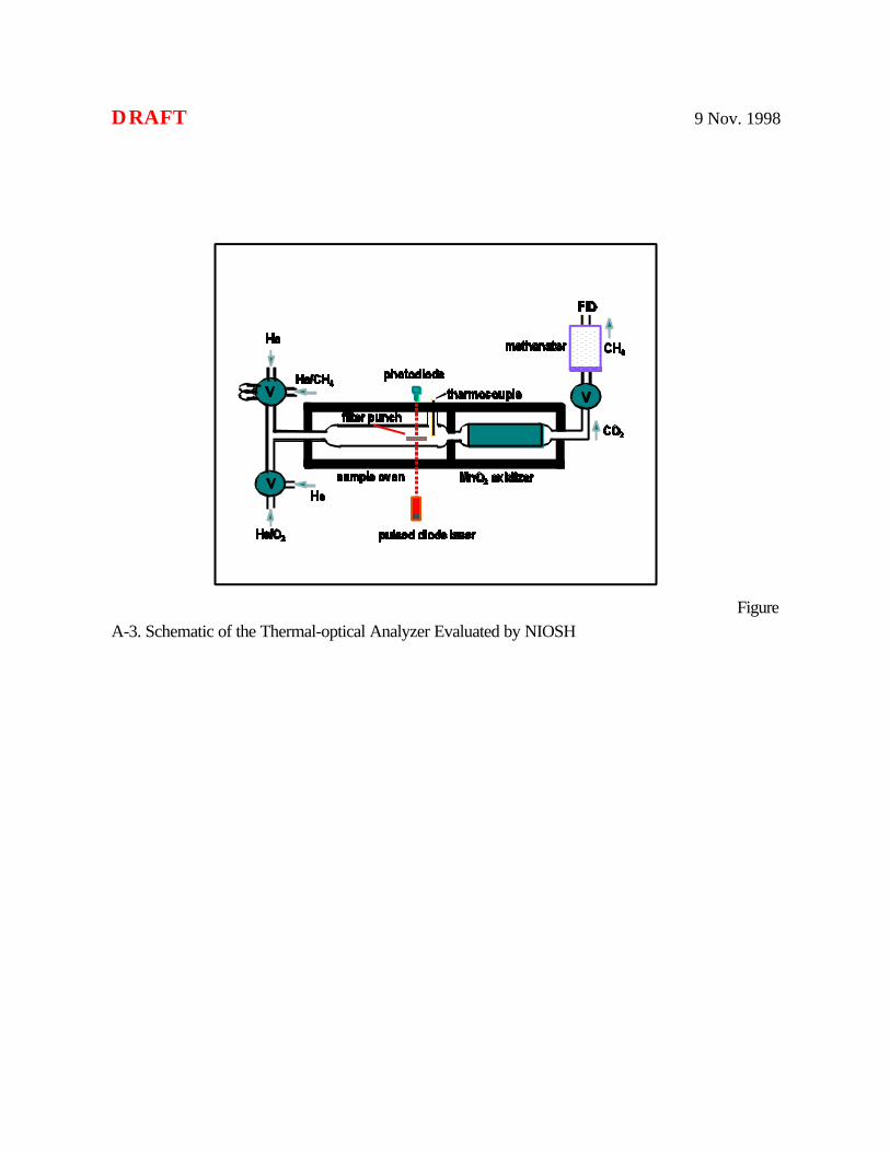
Organic and Elemental CarbonOrganic and elemental carbon collected on pre-baked quartz-fiber filters are determined by thethermal/optical reflectance method (TOR) (see SOP in Appendix B). In this method, a portion of thequartz-fiber filter is heated first in He to remove organic material and then in He with 2% oxygen toremove elemental carbon. The volatilized carbon is converted to CO and then to methane, which isdetected by an flame ionization detector. Optical reflectance of the sample is monitored to correct theTOR OC/EC analysis for possible charring during the highest temperature step in 100% He. Concentrations are determined by comparison to standards of known amounts. Atmosphericconcentrations are obtained based on the amount of filter used and the volume of air sampled.

Special Studies: XRF and Thermal Analysis for OC/ECLoss of Nitrate During XRF AnalysisAtmospheric pressure XRF, with secondary ion excitation will likely minimize loss of volatile speciese.g., nitrate and condensed SVOCs, during XRF analysis relative to vacuum XRF, thus, these filtersmight be able to be analyzed for nitrate, sulfate, and ammonium at a later date, or archived for other uses(e.g., QC check on final mass). However, most analytical laboratories use vacuum XRF and both

Part I, Page 16

primary and secondary excitation procedures, all of which would likely result in a significant loss ofvolatile species from the filter and limit it use for other analyses. Therefore, determining the effect ofvacuum XRF on volatile species is important for two reasons. First, the URG MASS sampler, asspecified from the manufacture uses the same filter to obtain mass, trace elements by XRF, and ions(sulfate and nitrate). If volatile species, i.e., nitrate and ammonium, are lost during vacuum XRF, thensubsequent determinations of those species will be biased by the amount lost. Secondly, the FRMsampler, in the compliance network is being used only for mass determination. If vacuum XRF does notbias the nitrate, ammonium, and organic carbon determinations, then these filters can be archived and, ifneeded re-weighed at a later time, or analyzed for sulfate, nitrate, and ammonium to provide a moredetailed chemical composition of the collected aerosol from the FRM sampler. One alternative wouldbe requiring atmospheric pressure XRF analysis of all Teflon filters, assuming it does not drive off semi-volatile species in the analysis process. The other alternative would be not using the filters for furtherchemical analysis or mass determinations. To examine the potential loss of volatile species from thecollected Teflon filter during vacuum XRF (see SOPs and Appendix B), 40 filters are analyzed byvacuum XRF, after atmospheric XRF analysis, and then analyzed for sulfate, nitrate, and ammonium byextraction and IC analysis as described below. These ions are compared to their concentrationscollected by the same sampler and by collocated samplers.

As just described, analysis of Teflon filters by atmospheric pressure XRF also may result in the loss ofvolatile species due to the phase equilibrium shifting to the gas phase as He passes over the sample. Teflonfilters previously analyzed by atmospheric pressure XRF are being analyzed for sulfate and nitrateconcentrations. These are being compared to nitrate and sulfate concentrations obtained by the samesampler and by collocated samplers.

TOR vs TOT Analysis for OC and ECTwo methods have been widely used for bulk analysis of OC and EC on quartz-fiber filters; thermaloptical reflectance (TOR) and thermal optical transmittance (TOT). TOT is the NIOSH 5040 methodthat is being used by the national laboratories for OC/EC determinations. At the names imply TORemploys reflectance to help adjust the OC/EC analysis for charring during the thermal evolution of OC,while TOT uses transmittance to accomplish the same objective. There are other differences betweenthe methods. For example, the temperature ramps are different and the maximum temperature used forobtaining OC and EC are different. For these reasons, investigators have observed differences betweenthe two methods for OC and EC determinations. Therefore, in this special study, a series of filters willbe analyzed by both methods, including standards of known concentrations.

Part I, Page 17

Splitting Filters for Multiple AnalysesAs described above, some of the filters are used for more then one analysis or the analytical methoditself requires only a section of the filter. For example, Teflon filters for anion and cation analysis aresplit in half so that each half can be extracted using the appropriate solution. Quartz-fiber filters aresectioned and only a small section (about 1 to 1.5 cm2) is used for analysis. As well, in the case of theURG chemical speciation sampler, the VAPS, and the FRM the filter is split in half, with one half usedfor ion analysis and the other for TOR analysis. The SOP for sample sectioning is found in Appendix B.

Filter and Denuder PreparationSeveral of the filters require pretreatment to lower blank levels and diffusion denuders need to be coatedwith a reactive substance to allow for efficient removal of specific gas phase species. For example,Teflon filters are equilibrated at specified T and RH as described earlier, quartz-fiber filters used forOC/EC analysis are baked for several hours (Chow, 1995) at 900 C to lower blank levels to 1 ug Ccm-2 of filter material, while nylon filters must be cleaned before use to ensure consistently low blanklevels if acceptance testing indicates variable blank levels or contamination greater then 1 ug NO3

- perfilter. Nylon filters are cleaned by soaking in a NO2CO3 solution followed by a thorough rinse using DIwater. Table I-3 lists the filters by sampler type and indicates general filter preparation needs. Denuders must be coated initially, cleaned or refurbished, and recoated as needed. As described inTable I-3, MgO denuders only require the initial coating as they are believed to have sufficient capacityfor the 20 day study and are not extracted for chemical analysis. The Na2CO3 coated denuder, requirescleaning and re-coating after every use, or at least after every three uses. In the VAPS, this denuderwas extracted after each sampling period and analyzed for HNO3. The XAD denuders, must berefurbished after every sampling period, and re-coated after every tenth sampling period.

Sampling Locations and RationaleSampling locations are identified based upon the following criteria. First, the statistical design requirestesting each sampler under different chemical atmospheres and varying environmental conditions. Secondly, locations are needed where PM sampling is ongoing with preference given to locations wherePM chemical speciation sampling is occurring at the time of the study. Finally, sufficient infrastructureneeds to be available with local support to assist with filter changing and sampler operations. Fourlocations were chosen that meet these criteria: Philadelphia, PA, Phoenix, AZ, Rubidoux, CA, andResearch Triangle Park, NC. Philadelphia represents a typical east coast situation where high sulfateand organic material are present in the aerosol, but nitrate is typically low (Pace, 1998). Phoenixrepresents an area with the potential for high crustal material, which typically is the dominant materialabove 2.5 Fm, but with a tail in the less than 2.5 Fm size range (Pace, 1998; Solomon et al., 1986). Phoenix also has a strong nitrate and organic material component. Rubidoux represents an area withvery high nitrate, moderate organic material, low sulfate, and relatively low crustal material (Solomon etal., 1989; SCAQMD, 1996). The RTP site is to allow for a more thorough evaluation of samplerperformance and provide a site where PM levels are near the lower limit of detection for the speciesmeasured by the samplers being tested.

Part I, Page 18

Of the four sites, Rubidoux is the prime site because it provides the most stringent test of the samplersfor examining collection efficiencies of nitrate and semi-volatile condensed organic compounds, has a fullcomplement of PM, gaseous, and meteorological sampling equipment, including full chemical speciationusing the SCAQMD’s PTEP sampler, and the characteristics of the air at Rubidoux have been wellcharacterized by several studies over the last decade (e.g., Solomon et al., 1989). Two sets of samplersare collocated at Rubidoux to obtain precision estimates. Table I-4 outlines the existing samplerequipment located at Rubidoux, CA. Table I-5 lists the existing equipment located at Phoenix, AZ. These two sites are well equipped to support this study with both additional PM measurements,meteorological measurements (the most important of which are relative humidity and temperature), andsupporting gas phase measurements, such as ozone, nitrogen oxides, and sulfur oxides. PM10 samplermeteorological data are collected at the Philadelphia site. At RTP, samplers were installed at the newNERL sampling platform; however, supporting data are not available at this site.

These sites represent Phase I of this program to evaluate the chemical speciation samplers for use in theNational Chemical Speciation Network. We recognize however, that the study is limited in scope, notonly geographically, but seasonally. Conditions that were not represented are the high sulfate season onthe east coast and areas with either high biogenic organic material or high wood smoke emissions. Thehighest season for crustal material in Phoenix is during the summer, thus, the samplers were notchallenged with the highest concentrations of crustal material. The samplers were not evaluated foroperations in either very cold or very hot conditions, nor under conditions of severe weather. Asdiscussed earlier, these other conditions will be tested during Phases II and III of this evaluation. Figures I-8 through I-11 show the samplers at each site.

Program ScheduleOverall Program ScheduleTable I-6 summarizes the overall schedule for this study. The schedule was driven by three criteria: 1) adraft report was due to OAQPS by the middle of March, 1998, 2) 20 sample sets would be collectedat each site to help ensure that a sufficient number of samples would be collected simultaneously on allsamplers to meet the statistical design objectives, and 3) the study could not begin until all five sets ofthe three chemical speciation samplers and the IMPROVE sampler were delivered to ORD (the originaldelivery date was August 15, 1998, and only MetOne met that schedule). The latter included deliveryof a sufficient number of spare parts, extra filter holders, and denuders to allow for every-other-daysampling. These three criteria uniquely define the schedule for the program and dictated that samplingmust be performed simultaneously at the four locations chosen for this study. Sampling was to beginaround September 1, 1998. However, all samplers and spare parts were not delivered until nearly theend of November 1998 (Andersen was the last sampler to arrive), which with seasonal holidays delayedthe start of sampling until nearly the middle of January, 1999. The due date for submission of the draftfinal report to OAQPS was then re-scheduled for the end of June 1999.

Sampling Schedule

Part I, Page 19

Sampling was conducted in January and February of 1999. Samplers were operated for 24-hr samplingperiods every other day, except at Rubidoux. Sampling at Rubidoux was every third day to samplesimultaneously with the PTEP sampler.

To meet the every other day sampling schedule, filters and holders were shipped overnight to thecontractor immediately after collection according to the sampling schedule illustrated in Table I-7. Filters, the XAD denuder in the VAPS, and all Na2CO3 denuders were shipped by overnight mail. Three full sets of filter holders and denuders were available for this purpose, which required continuousshipping of filters to and from the laboratory. This turned out to be a rigorous schedule to maintain withsite operators and laboratory personnel working 7 days per week. Delays only occurred when theovernight service failed to delivery the filters as expected.

Preliminary Evaluation and TrainingOnce samplers were received at EPA in Research Triangle Park, they were configured for use in thisfield study and underwent a quick shakedown. One representative from each manufacturer wasavailable to ensure proper assembly of their samplers and to train contractor personnel. The shakedownincluded, for example, running each sampler for two-12 to 24 hour periods to ensure that samplers wereturning on and off as expected, flow rate checks, flow control checks, leak checks, etc. Standardoperating procedures in the form of operating manuals were made available from the manufacturerswhen the samplers were delivered to RTP. The contractor prepared condensed installation andoperating SOPs for easy use by field and laboratory operators. A list of SOPs is given in Table I-2 andAppendix B.

Site Installation and DecommissioningAll sites were equipped with one of each of the three chemical speciation samplers, one IMPROVE,one VAPS, and one set of two FRM samplers. Rubidoux had a collocated second set of all samplersexcept the VAPS sampler. EPA contractor personnel installed the samplers at all sites, trained siteoperators at Rubidoux and Phoenix, and conducted initial systems and performance audits prior to thestart of the study. At the end of the study, EPA contractors performed a final audit and thendecommissioned the site and returned the equipment to EPA at Research Triangle Park, NC. A mid-study audit was also conducted.

Power and platforms were provided by the states or local districts. At Rubidoux and Phoenix, localstate or local district operators normally working at those sites operated the samplers. At Philadelphiaand RTP, the sites were operated by EPA contractors.

Part I, Page 20

Sampler Operation and Filter Shipping and StorageSamplers were operated according to the SOPs as given for each sampler and referenced Table 1-2and in Appendix B. Three full sets of filter holders and denuders were required for each sampler tomeet the rigorous schedule described above. The three sets of filter holders and denuders also allowedtime for these items to be shipped to the contractor for exchange, thus, removing site-to-site variabilityfor filter changing. Filters were shipped in coolers at reduced temperature with a max/min thermometer. Each cooler contained sufficient blue ice, sealed in plastic bags or some other closed system, to keep thefilters cool for 24-hours. At the field site, the filters were stored before and after sampling at reducedtemperatures in a refrigerator, especially after sample collection. Except for equilibration of filters formass determination, filters with collected aerosol were stored in sealed petri dishes at reducedtemperatures at or below freezing.

Quality Assurance/Quality Control (QA/QC)A thorough QA/QC effort was implemented for this study to ensure the quality of the data. Theseefforts included audits of the samplers prior to, during, and after the field program, even though the studywas only 2 months in duration. Laboratory quality assurance and control followed already establishedprocedures and included external audits of the analyzers in conjunction with ongoing studies.

Field QA/QCQuality assurance consisted of system and performance audits at the beginning, middle, and end of thestudy. These audits were conducted by contractor staff. Initial QA audits of the samplers wereperformed prior to the first sample if possible, or as quickly after the initiation of the program aspossible. A second set of system and performance audits was performed in the middle of the program,between the 8th and 10th sampling periods, depending on the site. A third set of audits was performedafter the last sample, but before decommissioning of the samplers by the EPA contractor. Initial systemaudits checked installation of the samplers, site setting, site operations and operators, and custodymanagement. Performance audits checked flow rates, check for vacuum leaks, and other performancecharacteristics of the samplers. Quality control consisted of checking flow rates before and after eachsample on every filter unless automatically logged by the sampler, maintaining appropriate operationslogs, checking filter holders and denuders prior to and after each sampling period, and other items asspecified on the data log sheets.

Part I, Page 21

Laboratory QA/QCLaboratory systems and performance audits were conducted for each species according to schedulesalready in place in the laboratories. Results will be reported to EPA staff in the contractors final report,which has not been received to date.

STATISTICAL ANALYSIS

Questions or Statistical Hypotheses Being TestedAs described above in the introduction, the primary objective of this study is to determine if there aredifferences among the three chemical speciation monitors for their estimation of the concentrations of thechemical components of PM2.5 mass. Comparisons also are made to two historical samplers(IMPROVE and VAPS) and to the FRM using these samplers as a relative reference. Referencestandards do not exist for any of the species, only for mass and that is defined by the FRM; therefore,this study is testing the equivalency of the samplers to each other, rather then comparing the samplers toa known value that provides an estimate of their accuracy.

There are three major questions to be addressed by this intercomparison study. 1. How do the concentrations of the measured chemical components as determined by the FRM

compare to those measured by the chemical speciation monitors?

2. Can FRM mass be reconstructed within expected uncertainties from the sum of the chemicalcomponents as measured by the chemical speciation monitors?

3. How well do the concentrations of the measured chemical components of PM2.5 from thevarious speciation samplers agree?

4. What are the causes of the differences, if they exist. Some are expected due to the differentmethods employed by the different samplers? and

5. What is the potential effect of different analytical methods on measured concentration of thechemical components of PM2.5. These include the effect of vacuum XRF vs. atmosphericpressure XRF on nitrate concentrations measured on Teflon filters and the effect of thermaloptical reflectance vs. thermal optical transmittance on OC/EC concentrations.

The following hypotheses are predicated on the assumption that the collection efficiency (slope of theefficiency curve and cutpoint) for the samplers in this study are essentially the same. Also, it is importantto establish the precision of the instruments and this was done by collocating samples at Rubidoux. While this provides only a limited assessment of the precision (one site, one time of the year, one set ofatmospheric conditions), it does provide a first cut estimate of the precision needed for the statisticalanalyses performed here. If for example, the precision is estimated at 50%, then determining differences

Part I, Page 22

among samplers is not as informative as if the precision were say 10-15%. As a benchmark, thecoefficient of variation for the differences in mass concentrations from collocated FRM instruments isrequired to be less than 10%, according to 40 CFR Part 58, Appendix A. Depending on the species,based on the authors’ prior experiences, we anticipate a range of precision from less than 10% to about30%.

In the following discussion, the phrase “speciation samplers” includes the Andersen RAAS, the URGMASS, the Met-One SASS, the IMPROVE, and the VAPS.

The following hypotheses are related to the first two questions, how do the samplers compare to theFRM and can FRM mass be reconstructed from the species measured by the speciation samplers. Foreach of these hypotheses, the concentrations, on a species-by-species basis, from each of the speciationsamplers is compared to the respective concentration from the FRM. The concentrations from thespeciation samplers are not compared to each other. The specific hypotheses are:

1. PM2.5 mass concentrations measured on the FRM by weighing a Teflon filter is compared toPM2.5 mass as measured by weighing filters collected by the Teflon filters in the chemicalspeciation monitors. The hypothesis is that the mass concentration from each of the speciationsamplers is not statistically different from the mass on the FRM filter. This is the starting point. The next eight hypotheses delve further into understanding why the mass concentrations do ordo not compare favorably.

2. PM2.5 trace elements or groups of trace elements determined on samples collected by the Teflonfilter in the FRM as determined by XRF are compared to trace elements determined on samplescollected on Teflon filters collected by the speciation samplers. The hypothesis is that there is nostatistical difference between the concentrations from each of the speciation samplers to thatdetermined from samples collected by the FRM. These concentrations should be comparablesince these species are stable.

3. PM2.5 sulfate on the FRM quartz filter is compared to sulfate on the Teflon (RAAS, SASS),quartz-fiber (MASS, VAPS), or nylon (IMPROVE) filters in the speciation samplers. Thehypothesis is that there is no difference between the concentrations from each of the speciationsamplers to that determined from samples collected by the FRM. These concentrations shouldbe comparable since sulfate is a stable species.

4. PM2.5 ammonium determined from samples collected by the quartz-fiber filter on the FRM iscompared to ammonium ion determined from samples collected on the Teflon (RAAS, SASS),quartz (MASS, VAPS), or nylon (IMPROVE) filters in the speciation samplers. The hypothesisis that there is no difference between the concentrations from each of the speciation samplers to

Part I, Page 23

that determined from samples collected by the FRM. These concentrations may not becomparable since ammonium is volatile when in the form of ammonium nitrate.

5. PM2.5 nitrate determined from samples collected on the quartz-fiber filter in the FRM iscompared to nitrate determined from samples collected on the Teflon (RAAS, SASS), quartz-fiber (MASS, VAPS), or nylon (IMPROVE) filters in the speciation samplers. The hypothesesis that there is no difference between the concentrations from each of the speciation samplers tothat determined from samples collected by the FRM. These concentrations should becomparable since the collection of nitrate on these filters should all be biased by the loss ofnitrate due to volatilization, with the exception of the IMPROVE.

6. PM2.5 nitrate on the FRM quartz filter is compared to nitrate on the nylon (RAAS, SASS,IMPROVE), or quartz+nylon (MASS, VAPS) filters in the speciation samplers. The hypothesisis that the nitrate from each of the speciation samplers is greater than or equal to the nitrate onthe FRM Teflon filter, due to negative artifacts in the FRM. This addresses questions about theamount of nitrate volatilized from the FRM Teflon filter.

7. PM2.5 elemental carbon (EC) determined on samples collected on quartz-fiber filters by theFRM is compared to EC determined on quartz-fiber filters collected by the chemical speciationsamplers. The hypothesis is that there is no difference between the concentrations from each ofthe speciation samplers to that from the FRM. These concentrations should be comparablesince elemental carbon is stable.

8. PM2.5 organic carbon (OC) determined on quartz-fiber filters collected by the FRM iscompared to OC determined on quartz fiber (MASS, RAAS, SASS, IMPROVE) filters in thespeciation samplers. The hypothesis is that there is no difference between the concentrationsfrom each of the speciation samplers to that determined from samples collected by the FRM. These concentrations should be comparable since as designed in this study, all the speciationsamplers potentially suffer from negative or positive artifacts.

9. PM2.5 OC determined on samples collected on the quartz-fiber filter in the FRM is compared toOC determined on samples collected on the quartz-fiber filter from the VAPS. The hypothesisis that OC collected by the FRM is greater then the OC collected by the VAPS denudedchannel if there are positive artifacts, or less than the VAPS denuded channel if there arenegative artifacts. No difference would be inconclusive.

The following hypotheses compare the concentrations of the chemical components determined onsamples collected by the chemical speciation samplers to address why there are differences amongmeasured concentrations, if they exist. For each of these hypotheses, only the concentrations from thespeciation samplers are compared.

Part I, Page 24

10. PM2.5 mass and chemical composition as determined according to the manufacturer’s guidelinesare compared among the speciation samplers. The hypothesis is that all species of interest arecomparable among the chemical speciation samplers when concentrations are determinedaccording to manufacturer’s guidelines.

11. PM2.5 mass concentrations determined by gravimetric analysis using Teflon filters are comparedamong the samplers. The hypothesis is that there is no difference in these masses.

12. PM2.5 trace element concentrations (individually or in groups) determined by XRF from samplescollected by Teflon filters are compared among the samplers. The hypothesis is that there is nodifference in these concentrations as these elements are stable during sampling and analysis.

13. PM2.5 nitrate concentrations determined from samples collected using nylon (RAAS, SASS,IMPROVE) or Teflon+nylon (MASS, VAPS) filters are compared among the samplers. Thehypothesis is that there is no difference in these concentrations.

14. PM2.5 sulfate determined from samples collected using Teflon (RAAS, SASS), quartz-fiber(MASS, VAPS), or nylon (IMPROVE) filters are compared among the samplers. Thehypothesis is that there is no difference in sulfate concentrations as sulfate is stable duringsampling and analysis. We also will look at sulfate estimated from XRF sulfur (S times 3 isapproximately equal to sulfate) to see how well XRF sulfur estimates sulfur determined by ICfrom both Teflon or quartz filters.

15. PM2.5 organic and elemental carbon determined from samples collected by quartz-fiber filterswhere no denuder is used is compared among the speciation samplers. Since the VAPS used adenuder, it will not be included in this hypothesis. The hypothesis is that the concentrations ofOC and EC are the same provided no denuder is employed.

16. PM2.5 organic and elemental carbon determined from samples collected by quartz-fiber filters,including speciation samplers where a denuder is used is compared among the samplers. Thehypothesis is that samplers that use denuders (VAPS) will have lower OC concentrations sincethe potential for positive artifact due to organic vapors has been minimized. Nothing can be saidabout negative artifacts.

17. PM2.5 ammonium determined from samples collected by the Teflon (RAAS, SASS), quartz-fiber (MASS, VAPS), or nylon (IMPROVE) filters are compared among the samplers. Thehypothesis is that the concentrations of ammonium are the same for all speciation samplers as allpotentially suffer from negative artifacts.

Part I, Page 25

18. Ammonium nitrate equilibrium is a function of temperature and relative humidity and thus, nitrateconcentrations measured on reactive filters behind a base coated denuder are compared as afunction of temperature and RH to determine if these factors bias sample collection. Thehypothesis is that there is no difference in the samplers as a function of temperature or RH.

19. Crustal related elements are typically associated with particles greater than 2.5 um AD,however, differences in the inlet the efficiency (slope and cutpoint) may result in differentconcentrations of crustal related material being measured by these samplers. The hypotheses isthat the crustal related material as determined from summing the oxides of Fe, Ca, and Si(Solomon et al., 1989) are not statistically different among the samplers. If differences areobserved they are related to the coarse particle mass as measured by the VAPS or by othercollocated PM10 monitors. Wind speed also is a variable of interest in this analysis.

The above hypotheses examine the first four major questions stated above. Statistical differences areexamined with in sites using primarily the paired t-test at alpha = 0.05. Added variability due to site-to-site variations in the chemical composition limit the paired t-test to individual sites, as missing data areminimized. The data also are examined by looking at means, time series analysis, regression analysis,difference analysis on a species by species basis relative to the FRM. Several tests are being conducted to examine the affect of different analytical methods on theconcentration of the species measured. These include the effect of vacuum XRF or atmospheric XRFon nitrate concentrations measured on the filter after XRF analysis and the use of TOR vs. TOT forOC/EC analysis as stated in the fifth question presented at the beginning of this section.

a. Examine the effect of vacuum vs. atmospheric pressure XRF on nitrate concentrationsmeasured on the Teflon filter after XRF analysis. The hypothesis is two fold. First,there will be a greater loss of nitrate from Teflon filters after vacuum XRF than afteratmospheric pressure XRF. Secondly, losses that occur during atmospheric pressureare minimized, such that nitrate measured after atmospheric pressure XRF is notdifferent than nitrate measured on a Teflon filter that has not undergone XRF analysis. Itis important to understand the magnitude of the loss of nitrate from Teflon filters aftervacuum or atmospheric XRF because the proposed design of the URG sampler has ionanalysis occurring after XRF analysis of the only Teflon filter in the system. There is alsogreat potential for the FRM Teflon filter to be used for XRF analysis and ion analysisafter mass determination to obtain additional speciation data at FRM sites.

b. Examine difference between OC and EC as measured by TOR and TOT. Thehypothesis is that these two methods are statistically not different from each other fordetermining OC and EC from samples collected on quartz-fiber filters. However,differences have been noted, especially with samples collected in areas with high woodsmoke emissions.

Part I, Page 26

Finally, the samplers will be evaluated in terms of their operational performance or practicality of use inthe field, that is, reliability, ruggedness, ease of use, and maintenance requirements. Field operatorswere asked to maintain detailed logs of their operational performance and they completed an extensivesurvey after the study on these issues. As well cost data are presented for the samplers and spare parts.

Part I, Page 27

Data Reporting Format

The concentrations for each analyte will be compiled as a flat ASCII file organized as follows:

1) Format ASCII text file with defined columns and rows.

2) Site ID’s:1 = Rubidoux2 = Phoenix3 = Philadelphia 4 = Research Triangle Park

3) Sampler ID’s:FRM - Teflon = FRM-TFRM - Quartz = FRM-QVAPS = VAPSMet One-SASS = METURG-MASS = URGAndersen RAAS = ANDImprove = IMP

4) Analytes (mass/m3)C-1 = PM2.5

C-2 = SO4

C-3 = NO3

C-4 = NH4

C-5 = OCC-6 = ECC-7 = S-XRFC-8.Cn = Individual metals – XRF

5) Reporting Duplicate Sampler Results (Rubidoux) Identify as “Repeat 1" and “Repeat 2".

Part I, Page 28

6) Limit of Detection (LOD) or MDL for Total Method (Sampling Plus Analysis)The LOD for mass is determined based on Federal Reference Method procedure (40 CFR,Part 50, Appendix L). The LOD sulfate, nitrate, and ammonium based on 3 time the noise inthe baseline noise in the chromatogram since field blanks were non-detectable, while for OCand EC it is based on three times the standard deviation of the field blanks. XRF limits ofdetection are based on propagating errors associated with the analytical method and flow rates. In general, LOD values were within the expected ranges.

Part I, Page 29

REFERENCES

Andersen. 1999 Operations Manual for the RAAS sampler. Andersen Instruments, GA.

Cahill, Thomas A. and Paul Wakabayashi. Compositional analysis ofsize-segregated aerosol samples. Chapter in the ACS book MeasurementChallenges in Atmospheric Chemistry. Leonard Newman, Editor. Chapter 7,Pp. 211-228 (1993).

Chameides, W.L., Lindsay, R.W., Richardson, J., Kiang, C.S., 1988. The role of biogenichydrocarbons in urban photochemical smog: Atlanta as a case study. Science 241, 1473-1475.

CFR 1997. National Primary and Secondary Ambient Air Quality Standards for Particulate Matter. Code Federal Regulations, 40 CFR 50.7. Published by the Office of Federal Register, NationalArchives and Records Administration.

Chow, J.C. 1995. Measurement Methods to Determine Compliance with Ambient Air Qualitystandards for suspended particles. Journal of the Air and Waste Management Association, 45:320.

Cui, W., J. Machir, L. Lewis, D.J. Eatough, and N.L. Eatough (1997). Fine Particulate OrganicMaterial at Meadview During the Project MOHAVE Summer Intensive Study, J. Air and WasteMgmt. Assoc., Volume 47.

Eatough, D.J., Tang, H.; Cui, W.; Machir, J. (1995). Determination of the Size Distribution andChemical Composition of Fine Particulate Semi-volatile Organic Material in Urban EnvironmentsUsing Diffusion Denuder Technology, Inhalation Toxicology, 1995, 7, 691-710.

Eldred, R.A., P.J. Feeny, and P.K. Wakabayashi. 1998a. The Major Components of PM2.5 atRemote Sites Across the United States. Proceedings of an International Speciality Conference – PM2.5:A Fine Particle Standard, Long Beach, CA, Jan. 28-30, A&WMA, Pittsburgh, PA, pp. 13-27.

Eldred, R.A., P.J. Feeny, P.K. Wakabayashi, J.C. Chow, E. Hardison. 1998b. Methodology forChemical Speciation Measurements in the IMPROVE Network. Proceedings of an InternationalSpeciality Conference – PM2.5: A Fine Particle Standard, Long Beach, CA, Jan. 28-30, A&WMA,Pittsburgh, PA, pp. 352-364.

EPA. 1998. Draft Supersites Conceptual Plan. Prepared for the Technical Subcommittee on FineParticle Monitoring of the Clean Air Scientific Advisory Committee by the Office of Air Quality Planning

Part I, Page 30

and Standards and Office of Research and Development. US EPA, Research Triangle Park, NC.Available at http://www.epa.gov/ttn/amtic/supsites.html.

EPA. 1999. Particulate Matter (PM2.5) Speciation Guidance Document. Monitoring and QualityAssurance Group, EMAD, OAQPS, Research Triangle Park, NC. Available athttp://www.epa.gov/ttn/amtic/pmspec.html.

EPA. 1997a. 62 FR 38761. National Ambient Air Quality Standards For Particulate Matter;Availability of Supplemental Information and Request For Comments, Final Rule, U.S. EnvironmentalProtection Agency, 40 Code of Federal Regulations, Part 50, Federal Register (62 FR 38761) , July18.

EPA 1997b. Revised Requirements For Designation of Reference and Equivalent Methods For PM2.5

and Ambient Air Quality Surveillance for Particulate Matter, Final Rule, U.S.Environmental Protection Agency, 40 Code of Federal Regulations Parts 53 and 58, Federal Register (62 FR 38763), July 18.

Hering, S.V., Lawson, D.R., Allegrini, I., Febo, A., Perrino, C., Possanzini, M., Sickles II, J.E., Anlauf,K.G., Wiebe, A., Appel, B.R., John, W., Ondo, J., Wall, S., Braman, R.S., Sutton, R., Cass, G.R.,Solomon, P.A., Eatough, D.J., Eatough, N.L., Ellis, E.C., Grosjean, D., Hicks, B.B., Womack, J.D.,Horrocks, J., Knapp, K.T., Ellestad, T.G., Paur, R.J., Mitchell, W.J., Pleasant, M., Peake, E.,MacLean, A., Pierson, W.R., Brachaczek, W., Schiff, H.I., Mackay, G.I., Spicer, C.W., Stedman,D.H., Winer, A.M., Biermann, H.W., and Tuazon, E.C., 1988. The Nitric Acid Shootout: FieldComparison of Measurement Methods. Atmospheric Environment 22, 1519-1539, Special Issue. Alsosee other papers in this special issue.

Hering, S. and Cass, G. 1999. The Magnitude of Bias in the Measurement of PM2.5 Arising fromVolatilization of Particulate Nitrate from Teflon Filter. JAWMA, 49, 725-733.

Hering, S. 1999. Program Plan for the Atlanta Supersites Study. Prepared by Aerosol Dynamics,Inc., Berkeley, CA.

Hidy, G.M., 1994. Atmospheric Sulfur and Nitrogen Oxides. Academic Press, San Diego, CA.

Koutrakis, P. 1998. Recommendations of the Expert Panel on the EPA Speciation Network. Reportto EPA, OAQPS. School of Public Health, Harvard University, Boston, MA (http://www.epa.gov/ttn/amtic/pmspec.html). http://www.epa.gov/ttnamti1/whatsnew.html

Mathai, C.V., John G. Watson, Jr., C. Fred Rogers, Judith C. Chow, Ivar, Tombach, Judith O.Zwicker, Thomas Cahill, Patrick Feeney, Robert Eldred, Marc Pitchford, and Peter K. Mueller. 1990.

Part I, Page 31

Intercomparison of ambient aerosol samplers used in western visibility and air quality studies. Environmental Science & Technology. Vol. 24, No. 7, pp. 1090-1099.

MetOne. 1999 Operations Manual for the SASS sampler. MetOne, Instruments. GA.

NARSTO. 1999. NARSTO Quality Systems Management Plan. Publication number 4785, Version1.0, September 30. NARSTO Quality Systems Science Center, Oak Ridge National Laboratory, OakRidge, TN. (Available from http://cdiac.esd.ornl.gov/programs/NARSTO/).

Pace, T. 1998. Composition of PM2.5 in Ambient Air. In Proceedings of an International SpecialityConference – PM2.5: A Fine Particle Standard, Long Beach, CA, Jan. 28-30, A&WMA, Pittsburgh,PA, pp. 3-12.

Pinto, J.P., R.K. Stevens, R.D. Willis, R. Kellogg, Y. Mamane, J. Novak, J. Santroch, I. Benes, J. Lenicek, and V. Bures. 1998. Chech Air Quality Monitoring and Receptor Modeling Study. Environ. Sci. Technol. 32, 843-854.

RTI. 1999. Quality Assurance Project Plan for Four-City PM2.5 ChemicalSpeciation Sampler Evaluation Study, RTI Project Number 07263-030. RTI, RTP,NC.

Russell, A.G. and G.R., Cass. 1986. Verification of a Mathematical Model for Aerosol Nitrate andNitric Acid Formation an its Use for control Measure Evaluation. Atmos. Environ., 20(2), 2,011-2,025.

SCAQMD. 1996. Final 1997 Air Quality Management Plan. South Coast Air Quality ManagementDistrict, Diamond Bar, CA.

Schauer, J.J., W.F. Rogge, L.M. Hildemann, L.M. Mazurek, G.R. Cass, and G.R. Simoneit. 1996. Source Apportionment of Airborne Particulate Matter Using Organic Compounds as Tracers. Atmos.Environ. 30, 3,837-3,855.

Schauer, J.J. 1998. Source Contributions to Atmospheric Organic Compound Concentrations:Emissions Measurements and Model Predictions. Chapter 10. Dissertation, California Institute ofTechnology, Pasadena, CA.

Mukerjee, S., W.D. Ellenson, R.G. Lewis, R.K. Stevens, M.C. Somerville, and D.S. Shadwick. 1997. An Environmental Scoping Study in the Lower Rio Grande Valley of Texas – 1. ComparativeAssessment of Air Sampling Methods. Environmental International 23(5), 61-628.

Part I, Page 32

Solomon, P.A. and J.L. Moyers. 1986. A Chemical Characterization of Wintertime Haze in Phoenix,Arizona. Atmospheric Environment, 20(1), 207-213.

Solomon, P.A., L. Salmon, T. Fall, and G.R. Cass. 1992. "The Spatial and Temporal Distribution ofAtmospheric Nitric Acid and Particulate Nitrate Concentrations in Los Angeles." Environ. Sci. Technol.26(8):1594-1601.

Solomon, P.A., T. Fall, L. Salmon, G.R. Cass, H.A. Gray, and A. Davidson. 1989. ChemicalCharacteristics of PM-10 Aerosols Collected in the Los Angeles Area. J. Air Pollut. Control Assn. 39(2):154-163.

Solomon, P.A., W. Mitchell, D. Gemmill, M. Tolocka, J. Suggs, J. Homolya, J. Rice, and S. Eberly. 1999. Field Program Plan For The PM2.5 Chemical Speciation Sampler Evaluation Study. Preparedby US EPA, ORD, NERL, Research Triangle Park, NC. Available athttp://www.epa.gov/ttn/amtic/pmspec.html

Sommerville, M.C., S. Mukerjee, D.L. Fox, and R.K. Stevens. 1994. Statistical Approaches in WindSector Analyses for Assessing Local Source Impacts. Atmos. Environ. 28, 3483-3493.

Stevens, R., J. Pinto, Y. Mamane, J. Ondov, M. Abdulraheem, N. Al-Majed, M. Sadek, W. Cofer,W. Ellenson, and R. Kellogg. 1993. Chemical and Physical Properties of Emissions from Kuwaiti OilFires. Water Sci. Techonl. 27, 223-233.

Teffera, S., S. Barbosa, and W.G. Bope. 1996. Design, testing, and implementation of a multi-channelsampler for use in an enhanced fine particulate monitoring program at the South Coast Air Basin. Papernumber 96-MP3.07. Proceedings Air & Waste Management Association, 89th Annual Meeting andExhibition, Nashville, TN, A&WMA, Pittsburgh, PA.

Part I Tables, Page 1

Table I-1. Analyte Listing for Speciation Sampler Intercomparison

AnalyticalMethod

Analyte(ConcentrationUnits)

Sampling Systems

MetOne

MASS RAAS IMPROVE FRM-T FRM-Q VAPS

Gravimetric PM2.5 Mass x x x x x - x

IonChromatography SO4

=, NO3-, NH4

+, x x x x - x x

Thermal/OpticalRef. Method OC/EC x x x x - x x

AtmosphericPressure XRF

S, Si, Ca, Mn, Fe, Cu, Zn, Pb,Groupings ofmetals, etc.,

x x x x x - x


Table I-2. List of Standard Operating Procedures for Field and Laboratory Efforts During the Chemical Speciation Monitor EvaluationStudy.

Field Related SOPs

SOP Prepared BySpiral Ambient Speciation Sampler MetOneReference Ambient Air Sampler AndersenMass Aerosol Speciation Sampler URG Corp.IMPROVE Sampler UC DavisVersatile Air Pollution Sample RTIPM2.5 Federal Reference Method RTIFilter Pack and Cassette Handling in the Field RTIDenuder Handling and Shipping in the Field RTIReceiving, Laboratory and Field RTIShipping at Reduced Temperatures RTI

Laboratory Related SOPs

SOP Prepared ByFilter Pack and Cassette Handling in the Lab RTIDenuder Preparation – Na2CO3 RTIDenuder Extraction – Na2CO3 RTIDenuder Preparation – MgO RTIDenuder Preparation – XAD RTIDenuder Regeneration – XAD RTIDenuder Extraction – XAD RTIPUF Cartridge Cleaning and Preparation RTIFilter Preparation – Nylasorb (nylon) RTIFilter Preparation – Teflon RTIFilter Preparation – Quartz-Fiber RTIAcceptance Testing of Filters RTIFilter Sectioning Procedures RTIFilter Extraction – Nylasorb RTIFilter Extraction -- Teflon RTIFilter Extraction – Quartz-Fiber RTIMass by Gravimetric Analysis1 RTIAnions by Ion Chromatography RTICations by Ion Chromatography RTIXRF – Atmospheric Pressure Mantech/NERLXRF – Under Vacuum DRI/RenoThermal-Optical Reflectance (TOR) DRI/RenoThermal-Optical Transmittance (TOT) Sunset LabsData Validation RTI

1 Federal Register for FRM.


Table I-3. Experimental Design Including Filter and Denuder Preparation.

SamplerFilter Type(Channel)

DenuderType Analysis Filter and Denuder Preparation

AndersenRAAS

Teflon (2)Teflon (3)

(2) Mass andelements1 (3) ions2

Filters are equilibrated before weighing Filters are wet with ethanol before extraction

Nylon (4) MgO Fine particle NO3

Nylon filters are cleaned before use and extractedin IC eluent; MgO denuders are not changed orcleaned during the study

Quartz (1) OC/EC Quartz filters are baked before use

Met-OneSASS

Teflon (1)Teflon (2)

(1) Mass andelements (2) ions

Filters are equilibrated before weighing Filters arewet with ethanol before extraction

Nylon (3) MgO Fine particle NO3-

Nylon filters are cleaned before use and extractedin IC eluent; MgO denuders are not changed orcleaned during the study

Quartz (4) OC/EC Quartz filters are baked before use

Quartz (5) OC/ECQuartz filters are baked before use; Carbondenuders need to be heat treated every 7 samples

URG MASS TeflonMass andelements

Filters are equilibrated before weighing

Nylon Na2CO3 Volatilized nitrateNylon filters are cleaned before use and areextracted in IC eluent; Na2CO3 denuders arecleaned and re-coated daily

Quartz OC/EC, ions Quartz filters are baked before use; Filters aresplit in half to allow for ion analysis

IMPROVE TeflonMass andelements


Nylon Na2CO3 Volatilized nitrate

Nylon filters are cleaned before use and areextracted in water since NH4

+ also is analyzed inthe extract; Na2CO3 denuders are cleaned and re-coated daily

Quartz OC/EC Quartz filters are baked before use

VAPS Teflon Na2CO3

Mass andelements Denuderfor HNO3

Filters are equilibrated before weighing Na2CO3

denuders are extracted and re-coated daily

Nylon Na2CO3 Volatilized nitrateNylon filters are cleaned before use. Nylon is thebackup filter in a Teflon/nylon filter pack

Quartz XAD-4Filter for OC/EC,ions Denuder forSVOCs

Quartz filters are baked before use; XAD-4denuders must be rinsed daily, re-coated every10 samples

FRM TeflonMass andelements


Quartz Ions and OC/ECQuartz filters are baked before use; Filters aresplit in half to allow for ion analysis

1. Elements refer to those obtained from XRF analysis, potential Na to Pb.

2. Ions include nitrate, sulfate and ammonium.


Table I-4. Measurements Made at Rubidoux, CA in Conjunction with the Chemical SpeciationSampler Evaluation Study.

Species Measurement Method Duration/Frequency1

PM2.5 and PM10 Mass andChemistry

Sierra Anderson DichotomousSamplers, PTEP Sampler

24 hrs/1 in 3 days

PM2.5 Elemental Carbon Magee Scientific aethalometer witha Harvard Impactor PM2.5 inlet

5 minute average, C

Light scattering Optec nephelometer 1 hour average, C

PM2.5 EC/OC Rupprecht & Patashnick TotalCarbon Analyzer

1 hour average, C

PM10 Mass Rupprecht & Patashnick PM10

Federal Equivalent Method TEOM1 hour average, C

Methane/NMHC TEI hydrocarbon analyzer 1 hour average, C

NOx/NOy TEI NOx/NOy analyzers 1 hour average, C

O3 One Dasibi ozone analyzer 1 hour average, C

CO TEI CO analyzer 1 hour average, C

NO, NO2, NOx TEI NOx analyzer 1 hour average, C

Wind Speed AGL 1 hour average, C

Wind Direction AGL 1 hour average, C

Standard Deviation of WindDirection

AGL 1 hour average, C

Air Temperature 2 meters AGL, nephelometer height 1 hour average, C

Relative Humidity 2 meters AGL, nephelometer height 1 hour average, C

Delta Temperature C

1 O6-one in six days; C-continuous; D-Daily; OD-Every other day.


Table I-5. Measurements Made at Phoenix, AZ in Conjunction with the Chemical Speciation SamplerEvaluation Study.

Species Measurement Method Duration/Frequency2

PM2.5, Coarse PM, & PM10

Mass and Chemistry

4 - Sierra Anderson DichotomousSamplers

6 and 24 hours/O6, (2 w/ quartz, 2 w/Teflon filters)

PM2.5, Coarse PM, & PM10

Mass and Chemistry

2 - IMPROVE 25mm 4-modulesamplers

24 hours/OD, (each w/ Teflon,nylon, quartz, & PM10 Teflon filters,respectively)

PM2.5

Elemental Carbon / LightAbsorption

2 - Magee Scientific aethalometers,each with a Harvard Impactor PM2.5

inlet

5 minute average/C

Ambient light scattering Optec nephelometer (NGN-2) 1 hour average/C

PM2.5 EC/OC Rupprecht & Patashnick TotalCarbon Analyzer

1 hour average/C

PM10 Mass Rupprecht & Patashnick PM10

Federal Equivalent Method TEOM1 hour average/C

Methane/NMHC TEI hydrocarbon analyzer 1 hour average/C

NOx/NOy TEI NOx/NOy Trace level analyzers 1 hour average/C

O3 Dasibi O3 analyzer 1 hour average/C

CO TEI CO analyzer 1 hour average/C

NO, NO2, NOx TEI NOx analyzer 1 hour average/C

SO2 Monitor Labs SO2 analyzer 1 hour average/C

Wind Speed 10 meters AGL 1 hour average/C

Wind Direction 10 meters AGL 1 hour average/C

Standard Deviation of WindDirection

10 meters AGL 1 hour average/C

1 O6-one in six days; C-continuous; D-Daily; OD-Every other day.


Table I-6. Overall Planned Study Schedule1.

Date Deliverable

1998

November 10 Standard operating procedures received from the 3 chemical speciation samplermanufacturers and for the IMPROVE and VAPS samplers

October 1-Nov. 20 Sites prepared for sampler installation. Power and platforms installed as needed toaccommodate all samplers (see Tables 1 and 2 for listing of samplers at each site).

Nov 1 - 30 Samplers will undergo an evaluation and RTP field personnel will be trained on installation,operation, and quality control

Nov 12-24 External review by the expert peer-review panel on chemical speciation.

Nov 20-Dec 10 Samplers shipped to sampling sites and local operators trained.

Dec 8-Dec 12 Systems and performance audits performed with help from local agency (Rubidoux andPhoenix)

Dec 14 First day of sampling. (Rubidoux and Phoenix)

1999

Jan 4-Jan 5 Systems and performance audits performed with help from local agency (Phoenix andPhiladelphia)

Jan 6 First day of sampling (Philadelphia and RTP)

Jan.1-4 Systems and performance audits performed with help from local agency.(optional)Chemicalanalysis of first half of samples should be started.

March 1 Last day of sampling. Systems and performance audits performed with help of local agency.

March 2-5 Decommission sites.

March 20 Chemical analyses complete.

April 15 Level II data delivered to EPA for all chemical analyses.

April 15-May 1 EPA reviews data and begins initial statistical analysis 2

May 1-May-15 All final statistics prepared, including plots, tables, and figures

May 15-May 30 Prepare report and submit to internal NERL review group for comments

June 15 Address comments from internal review group

June 25 Provide OAQPS with draft report.

1. Actual schedule for data delivery was delayed. However, OAQPS also delayed implementation of samplers andboth schedules then coincided.

2. Detailed initial results are forwarded to OAQPS at this point or earlier.


Table I-7. Field Operations Sampling Schedule.

Sample Day Rubidoux Phoenix Philadelphia RTP

1 1/6/99 1/6/99 1/17/99 1/15/99

2 1/9/99 1/8/99 1/19/99 1/17/99

3 1/15/99 1/14/99 1/21/99 1/19/99

4 1/18/99 1/16/99 1/23/99 1/21/99

5 1/21/99 1/18/99 1/25/99 1/23/99

6 1/24/99 1/20/99 1/27/99 1/25/99

7 1/27/99 1/22/99 1/29/99 1/27/99

8 1/30/99 1/24/99 1/31/99 1/29/99

9 2/2/99 1/26/99 2/2/99 1/31/99

10 2/5/99 1/28/99 2/4/99 2/2/99

10 (blank) 2/9/99 1/29/99 2/5/99 2/5/99

11 2/11/99 2/3/99 2/8/99 2/6/99

12 2/14/99 2/5/99 2/10/99 2/8/99

13 2/17/99 2/7/99 2/12/99 2/10/99

14 2/20/99 2/9/99 2/14/99 2/12/99

15 2/23/99 2/11/99 2/16/99 2/14/99

16 2/26/99 2/13/99 2/18/99 2/16/99

17 3/1/99 2/15/99 2/20/99 2/18/99

17 (blank) 3/2/99 n/a n/a n/a

18 n/a 2/17/99 2/22/99 2/20/99

19 n/a 2/19/99 2/24/99 2/22/99

20 n/a 2/21/99 2/26/99 2/24/99

20 (blank) n/a 2/24/99 2/27/99 2/25/99

F:\USER\BMILLAR\amticweb\fourcities\02 Part I Tables v8-f.wpd

Part I Figures, Page 1

Teflon Filter Teflon Filter Nylon Filter

Cyclone Fractionator

Pump

Air

Flo

w

OC/EC Mass,Elements by XRF

SO42-, NO3

-, NH4+ Fine Particle

Nitrate

Inlet

Quartz Filter

7.3

Lpm

16.7

Lpm

16.7

Lpm

7.3

Lpm

MgO

Den

uder

4 32 1

Cyclone Fractionator

Manifold Manifold

SamplerHousing

Figure I-1a. Schematic of the Andersen RAAS Sampler.


Figure I-1b. Picture of the Andersen RAAS Sampler Deployed in the Field at RTP.


EmptyTeflon Filter Nylon Filter

EmptyQuartz FilterQuartz Filter

Quartz FilterQuartz FilterEmpty

Teflon Filter

Empty

Spiral Impactor

Empty

Spiral Impactor Spiral Impactor Spiral Impactor

Empty

Spiral Impactor

Flo

w m

eter

Flo

w m

eter

Flo

w m

eter

Flo

w m

eter

Flo

w m

eter

p u m p

Mass ,Elements b y X R F

SO 42-, NO 3

-,N H 4

+Fine Part icle

NitrateOC/ E C Repl ica te OC/EC

EmptyMgO Coated

Al HoneycombDenuder

Air

Flo

w

6.7 L

pm

6.7 L

pm

6.7 L

pm

6.7 L

pm

6.7 L

pm

1 432 5

Figure I-2a. Schematic of the MetOne SASS Sampler.


Figure I-2b. Picture of MetOne Sampler Deployed in the Field at RTP. Left – Inlet, Filter Holders, and Meteorological Sensor. Right-Pumpbox.


Size selectiveInlet (PM10)

Sodium CarbonateDenuder

Nylasorb FilterMass, Elements by XRF

Volatilized Nitrate

Pump

HNO3

Air

Flo

w

WINSImpactor

OC/EC, SO4

2-, NO3-,

NH4+

Teflon Filter


Quartz Filter

Pump

16.7

Lpm

WINSImpactor

Sampler Housing

Sampler Housing

MASS 400 MASS 450

Figure I-3a. Schematic of the URG MASS Sampler.


Figure I-3b. Picture of the URG MASS Sampler Deployed in the Field at RTP.


Mass,Elements by XRF

Size selectiveInlet

Pump

Size selectiveCyclone

Teflon Filter

SO42-, NO3

-,NH4+

Size selectiveInlet

Pump

OC/EC

Size selectiveInlet

Pump


Quartz Filter

Nylon Filter

Na 2C

O3 D

enud

er

Air

Flo

w

22.7

Lpm


SamplerHousing

SamplerHousings

1 2 3

Figure I-4a. Schematic of the IMPROVE Sampler.


Figure I-4b. Picture of the Filter Position, Control Box, and Timer for One of the Three Modules of the IMPROVE Sampler as Deployed inthe Field at RTP.


Quartz Filter

Size SelectiveInlet

Teflon Filter

XA

D-2

Den

uder

VI

Air

Flo

w

Pump Pump Pump

Mass, Elements by XRF

Coarse Particle Mass A. SVOCs B. OC/EC,

SO42-, NO3

-,NH4+

VI = virtual impactor

Teflon Filter

15 L

pm

33 L

pm

3 L

pm

15 L

pm

Na 2

CO

3Den

uder

Nylon Filter

A

B

SamplerHousing

2

1

3

Figure I-5a. Schematic of the VAPS Sampler.


Figure I-5b. Picture of VAPS Sampler Deployed in the Field at RTP. Left – VAPS Filter Box Showing XAD Denuder on Right and SodiumCarbonate Coated Annular Denuder on Left. Right – Pump Box and Dry Gas Meters for Monitoring Flow.


OC/EC,SO4

2-, NO3-,NH4

+


Pump

WINSImpactor

Quartz Filter

Mass,Elements by XRF


Pump

WINSImpactor

Teflon FilterAir

Flo

w

16.7

Lpm

SamplerHousing

Figure I-6a. Schematic of the Federal Reference Method Samplers


Andersen BGI R&P

Figure I-6b. Picture of FRM Samplers Deployed in the Field at RTP.


Figure I-7. Schematic of the SCAQMD Multi-Channel Fine Particulate Sampler.


Figure I-8. Top – Samplers on the Platform at Rubidoux, CA. Bottom – View of the SamplingPlatform and Surrounding Area at Rubidoux, CA.


Figure I-9. Sampling Platform at Phoenix, AZ.


Figure I-10. Philadelphia Sampling Site. Top – Roof View. Bottom –View From the Road.

C:\WINDOWS\TEMP\03 Part I FIGURES v8-f.wpd Part I Figures, Page 17

Figure I-11. Research Triangle Park Sampling Site.

Part II

Results, Discussion, Conclusions, and Implications

Part II, Page ii

Table of Contents – Part II

Table of Contents – Part II . . . . . . . . . . . . . . . . . . . . . . . . . . . . . . . . . . . . . . . . . . . . Part II, Page ii

List of Tables – Part II . . . . . . . . . . . . . . . . . . . . . . . . . . . . . . . . . . . . . . . . . . . . . . . Part II, Page v

List of Figures – Part II . . . . . . . . . . . . . . . . . . . . . . . . . . . . . . . . . . . . . . . . . . . . . Part II, Page vi

RESULTS . . . . . . . . . . . . . . . . . . . . . . . . . . . . . . . . . . . . . . . . . . . . . . . . . . . . . . . . Part II, Page 1

Quality Assurance Results . . . . . . . . . . . . . . . . . . . . . . . . . . . . . . . . . . . . . . . . . . . Part II, Page 1Performance Audit Methods and Verification . . . . . . . . . . . . . . . . . . . . . . . . . Part II, Page 1

Flow Rate Audit Equipment . . . . . . . . . . . . . . . . . . . . . . . . . . . . . . . . Part II, Page 1Barometric Pressure Audit Equipment . . . . . . . . . . . . . . . . . . . . . . . . . Part II, Page 1Temperature Audit Equipment . . . . . . . . . . . . . . . . . . . . . . . . . . . . . . Part II, Page 1

Field Audit Results . . . . . . . . . . . . . . . . . . . . . . . . . . . . . . . . . . . . . . . . . . . . . Part II, Page 2Limits of Detection . . . . . . . . . . . . . . . . . . . . . . . . . . . . . . . . . . . . . . . . . . . . . Part II, Page 3Field Blanks . . . . . . . . . . . . . . . . . . . . . . . . . . . . . . . . . . . . . . . . . . . . . . . . . . Part II, Page 3Precision . . . . . . . . . . . . . . . . . . . . . . . . . . . . . . . . . . . . . . . . . . . . . . . . . . . . Part II, Page 4Data Validation . . . . . . . . . . . . . . . . . . . . . . . . . . . . . . . . . . . . . . . . . . . . . . . Part II, Page 4

Level 1a Data Validation . . . . . . . . . . . . . . . . . . . . . . . . . . . . . . . . . . Part II, Page 4Level 1b Data Validation . . . . . . . . . . . . . . . . . . . . . . . . . . . . . . . . . . Part II, Page 5Level 2b Data Validation . . . . . . . . . . . . . . . . . . . . . . . . . . . . . . . . . . Part II, Page 5Data Capture . . . . . . . . . . . . . . . . . . . . . . . . . . . . . . . . . . . . . . . . . . . Part II, Page 5

Chemical Characteristics of PM 2.5 . . . . . . . . . . . . . . . . . . . . . . . . . . . . . . . . . . . . . Part II, Page 7Chemical Components Reported in the 4 City Study Database . . . . . . . . . . . . Part II, Page 7PM2.5 and Chemical Components Collected by the FRM . . . . . . . . . . . . . . . . Part II, Page 7Volatilization of Aerosol Nitrate . . . . . . . . . . . . . . . . . . . . . . . . . . . . . . . . . . Part II, Page 10

Statistical Analysis . . . . . . . . . . . . . . . . . . . . . . . . . . . . . . . . . . . . . . . . . . . . . . . . Part II, Page 11Means of PM2.5 Mass and Major Chemical Components . . . . . . . . . . . . . . . Part II, Page 11

Explanations of Anomalous Data . . . . . . . . . . . . . . . . . . . . . . . . . . . Part II, Page 11Comparison of Means Among Samplers . . . . . . . . . . . . . . . . . . . . . . Part II, Page 13Comparison To Performance Criteria . . . . . . . . . . . . . . . . . . . . . . . . Part II, Page 14

Time Series Analysis . . . . . . . . . . . . . . . . . . . . . . . . . . . . . . . . . . . . . . . . . . Part II, Page 15Regression Analysis . . . . . . . . . . . . . . . . . . . . . . . . . . . . . . . . . . . . . . . . . . . Part II, Page 16

Mass . . . . . . . . . . . . . . . . . . . . . . . . . . . . . . . . . . . . . . . . . . . . . . . . Part II, Page 16Sulfate . . . . . . . . . . . . . . . . . . . . . . . . . . . . . . . . . . . . . . . . . . . . . . . Part II, Page 17Nitrate . . . . . . . . . . . . . . . . . . . . . . . . . . . . . . . . . . . . . . . . . . . . . . . Part II, Page 17Ammonium . . . . . . . . . . . . . . . . . . . . . . . . . . . . . . . . . . . . . . . . . . . Part II, Page 18

Part II, Page iii

Organic and Elemental Carbon . . . . . . . . . . . . . . . . . . . . . . . . . . . . . Part II, Page 18Trace Elements . . . . . . . . . . . . . . . . . . . . . . . . . . . . . . . . . . . . . . . . Part II, Page 19

T-TEST Results . . . . . . . . . . . . . . . . . . . . . . . . . . . . . . . . . . . . . . . . . . . . . . Part II, Page 19Results from the Paired T-Tests . . . . . . . . . . . . . . . . . . . . . . . . . . . . Part II, Page 21

Paired T-Test Results for FRM and Andersen Samplers . . . . Part II, Page 22Paired T-Test Results for FRM and MetOne Samplers . . . . . Part II, Page 22Paired T-Test Results for FRM and IMPROVE Samplers

. . . . . . . . . . . . . . . . . . . . . . . . . . . . . . . . . . . . . . . . Part II, Page 22Paired T-Test Results for FRM and URG Samplers . . . . . . . Part II, Page 22Paired T-Test Results for the FRM and VAPS Samplers . . . Part II, Page 23

Results from the ANOVA on Particle Nitrate Data . . . . . . . . . . . . . . . . . . . . Part II, Page 23Aerosol Nitrate . . . . . . . . . . . . . . . . . . . . . . . . . . . . . . . . . . . . . . . . . . . . . . Part II, Page 23Organic and Elemental Carbon . . . . . . . . . . . . . . . . . . . . . . . . . . . . . . . . . . . Part II, Page 25

Denuded vs Non-Denuded Organic Carbon Results . . . . . . . . . . . . . Part II, Page 25Comparison between TOR and TOT for OC and EC in PM2.5 . . . . . Part II, Page 26

Loss of Nitrate During Vacuum XRF Analysis . . . . . . . . . . . . . . . . . . . . . . . Part II, Page 27

Field Experience with the Speciation Samplers . . . . . . . . . . . . . . . . . . . . . . . . . . Part II, Page 28Andersen RAAS . . . . . . . . . . . . . . . . . . . . . . . . . . . . . . . . . . . . . . . . Part II, Page 29Met One SASS . . . . . . . . . . . . . . . . . . . . . . . . . . . . . . . . . . . . . . . . . . . . . . Part II, Page 29URG MASS . . . . . . . . . . . . . . . . . . . . . . . . . . . . . . . . . . . . . . . . . . . . . . . . Part II, Page 29IMPROVE . . . . . . . . . . . . . . . . . . . . . . . . . . . . . . . . . . . . . . . . . . . . . . . . . Part II, Page 30VAPS . . . . . . . . . . . . . . . . . . . . . . . . . . . . . . . . . . . . . . . . . . . . . . . . . . . . . Part II, Page 30FRM . . . . . . . . . . . . . . . . . . . . . . . . . . . . . . . . . . . . . . . . . . . . . . . . . . . . . . Part II, Page 30

Sampler Costs and Related Spare Parts . . . . . . . . . . . . . . . . . . . . . . . . . . . . . . . Part II, Page 31

DISCUSSION . . . . . . . . . . . . . . . . . . . . . . . . . . . . . . . . . . . . . . . . . . . . . . . . . . . . Part II, Page 32

Expectations . . . . . . . . . . . . . . . . . . . . . . . . . . . . . . . . . . . . . . . . . . . . . . . . . . . . . Part II, Page 32

Major Questions Addressed . . . . . . . . . . . . . . . . . . . . . . . . . . . . . . . . . . . . . . . . . Part II, Page 32Q1. How well do PM2.5 mass and the chemical components of mass agree between the

FRM and the chemical speciation samplers tested in this study? . . . . . . . . . . . . . . . . . . . . . . . . . . . . . . . . . . . . . . . . . . . . . . . . . . . . Part II, Page 33

Q2. How well can the FRM mass be reconstructed by summing the chemical componentsmeasured by the speciation samplers. . . . . . . . . . . . . . . . . . . . . . . . . Part II, Page 34Specific Hypotheses Related to Questions Q1 and Q2 . . . . . . . . . . . Part II, Page 35

Denuded vs Non-Denuded Organic Carbon Results . . . . . . . Part II, Page 38Q3. How well do the measured concentrations from the various speciation samplers agree?Part II, Page 39

Part II, Page iv

Q4. What are the causes of the differences among the speciation samplers for measuredconcentrations of mass and the components of mass if they exist.. . . . . . . . . . . . . . . . . . . . . . . . . . . . . . . . . . . . . . . . . . . . . . . . . . . . Part II, Page 39

Specific Hypotheses Related to Questions Q3 and Q4 . . . . . . . . . . . Part II, Page 39

SUMMARY AND CONCLUSIONS . . . . . . . . . . . . . . . . . . . . . . . . . . . . . . . . . . Part II, Page 44Site Characteristics . . . . . . . . . . . . . . . . . . . . . . . . . . . . . . . . . . . . . . . . . . Part II, Page 44Operations . . . . . . . . . . . . . . . . . . . . . . . . . . . . . . . . . . . . . . . . . . . . . . . . . Part II, Page 44Measurement Performance . . . . . . . . . . . . . . . . . . . . . . . . . . . . . . . . . . . Part II, Page 45Implications . . . . . . . . . . . . . . . . . . . . . . . . . . . . . . . . . . . . . . . . . . . . . . . . Part II, Page 45

Nitrate . . . . . . . . . . . . . . . . . . . . . . . . . . . . . . . . . . . . . . . . . . . . . . . Part II, Page 45Carbon . . . . . . . . . . . . . . . . . . . . . . . . . . . . . . . . . . . . . . . . . . . . . . Part II, Page 46

REFERENCES . . . . . . . . . . . . . . . . . . . . . . . . . . . . . . . . . . . . . . . . . . . . . . . . . . . Part II, Page 47

Tables – Part II . . . . . . . . . . . . . . . . . . . . . . . . . . . . . . . . . . . . . . . . . . . . . . . Part II Tables, Page 1

Figures – Part II . . . . . . . . . . . . . . . . . . . . . . . . . . . . . . . . . . . . . . . . . . . . . Part II Figures, Page 1

Part II, Page v

List of Tables – Part IITable II-1. Summary of Flow Audit Results.Table II-2a. Limits of Detection in ng/m3.Table II-2b. Average Field Blank Data for All Species and Samplers Averaged Across All Sites In

Atmospheric Concentrations.Table II-2c. Precision (as % CV) Achieved by FRM and Speciation Samplers Based on Results

from the Collocated Samplers at Rubidoux.Table II-3. Valid Data Capture in Percent by Sampler and Major Species.Table II-4. Summary of Problems Encountered In the Field During Operations of Sampler

Evaluated in this Study.Table II-5. Species Concentration Data for the FRM at Each Location of the 4-City Study.Table II-6. Estimated PM2.5 Mass Balance of Species versus Measured PM2.5 Mass (ug/m3) for

the FRM at Each Site.Table II-7. Average Volatilized Nitrate (NO3V) in ug/m3 Observed for Each Sampler at Each

City.Table II-8a. Mean Analyte Concentrations for Each Sampler at All Sites.Table II-8b. Ratio of Speciation Sampler to FRM for Chemical Components by Site.Table II-9. Regression Statistics of FRM (x-axis) versus Speciation Samplers (y-axis) for All Sites,

Samplers, and Major Species.Table II-10. Results from the Paired t-Tests Between the Speciation Samplers and FRM Samplers

for Each Analyte/Site.Table II-11. Results from the ANOVA for Examining Equivalency Among the Samplers for

Particulate Nitrate.Table II-12a. Nitrate Concentrations (ug/m3) Measured on Teflon (T) or Quartz-Fiber (Q) Filters by

Sampler Type Averaged Over the Study Period.Table II-12b. Total Particle Nitrate Concentrations (ug/m3) Measured by Each Sampler Averaged

Over the Study Period.Table II-12c. Volatilized Nitrate Concentrations (ug/m3) Measured by Each Sampler Averaged Over

the Study Period.Table II-12d. Sulfate Concentrations (ug/m3) Measured on Teflon (T) or Quartz-Fiber (Q) Filters

Averaged Over the Study Period.Table II-13a. Nitrate Concentrations (ug/m3) Measured on Teflon (T) or Quartz-Fiber (Q) Filters

Averaged Over the Study Period.Table II-13b. Total Particle Nitrate Concentrations (ug/m3) Measured by Different Denuder-Filter

Pack Methods Averaged Over the Study Period.Table II-13c. Volatilized Nitrate Concentrations (ug/m3) Measured by Different Denuder-Filter Pack

Methods Averaged Over the Study Period.Table II-13d. Sulfate Concentrations (ug/m3) Measured on Teflon and Quartz Filters Averaged Over

the Study Period.Table II-14. Loss of Nitrate Resulting from Analysis of Teflon Filter by Vacuum XRF.Table II-15. Summary of Site Operators Surveys Regarding Speciation Sampler Setup and

operation.Table II-16. Recommended Spare Parts and Supplies for Use of Chemical Speciation Samplers and

FRM Used in the Chemical Speciation Evaluation Study.

Part II, Page vi

List of Figures – Part II

Figure II-1. Frequency Distributions, Given as Box and Whisker Plots of PM2.5 Species at Each ofthe Four Cities Studies

Figure II-2. Chemical Mass Balance of PM2.5 at Each City.Figure II-3. Time Series Plots.Figure II-4. Regression Analysis Plots.Figure II-5. Denuded and Non-Denuded OC Samples as a Function of the TOR Carbon Fractions.Figure II-6. Organic Carbon concentrations from FRM and VAPS versus Total FRM PM2.5

Mass.Figure II-7. Organic and Elemental Carbon as a function of Face Velocity. Figure II-8. Loss of Aerosol Nitrate from Teflon filters Due to Vacuum XRF Analysis.

Part II, Page 1

RESULTSQuality Assurance Results

Performance Audit Methods and Verification

As part of the overall field evaluation of the candidate speciation samplers, periodic performanceevaluations were conducted at each of the four sampling sites. Following the initial calibration of eachsampler and site installation, a pre-sampling evaluation was conducted to ensure that each sampler wasoperating according to manufacturer’s specifications. The pre-sampling evaluation consisted of single-point verification of each sampler’s operating flow rate and ambient temperature, and pressuremeasurements. Subsequent mid- and post-study performance evaluations consisted of similarevaluations. Pre-sampling audits were typically conducted approximately one day prior to the initiationof Run 1, while the mid-study audit was conducted following Run 10. The final site audit wasconducted shortly after the last sampling period.

Flow Rate Audit Equipment

The flow rate audit consisted of a single-point measurement conducted at the operational flow rate ofeach channel for each sampler. Depending upon the sampler and the specific channel being audited,one of two flow audit devices was typically used. A Chinook Engineering Streamline flow transferstandard (FTS #980819) was used for the majority of the channel audits. Prior to its purchase, theStreamline FTS was calibrated by the manufacturer against a set of precision NIST traceable criticalflow venturis. Following its purchase, its performance was verified in the laboratory at RTI. Thesecond in field flow audit device used in this study was a Schlumberger dry gas meter. Its traceabilitywas established in the laboratory using EPA Method 40 CFR60, Appendix A, Method 5, Section 7.

Barometric Pressure Audit Equipment

Laboratory calibrations and field audits of speciation sampler pressure sensors were conducted using aPSI Tronix Model PG 2000 digital pressure gauge. Laboratory validation of the Model PG 2000'sresponse was obtained using a certified mercury barometer previously adjusted to local stationpressure.

Temperature Audit Equipment

Two instruments were used for laboratory calibration and auditing of speciation sampler ambienttemperature response. A Tegum Model 847 thermo-calibrator was used to calibrate and audit Type Kthermocouples used in some speciation sampler designs. Other samplers were audited using a FlukeModel 8022A digital multi-meter in conjunction with a Model 80T-150U temperature probe. Traceability of the Fluke probe was established using a traceable Hewlett Packard quartz probe (S/N725A Model 2833A).

Part II, Page 2

Field Audit Results

Results of the pre-, mid-, and post-study field flow rate audit results are summarized in Table II-1. Values are given for flow audit results that were outside of < 10% and > 10%, all othersare within ±10% of the audit device. All flow channels were audited as well as audits of all temperatureand pressure measurement devices associated with each sampler. Pressure and temperature auditresults for the IMPROVE and VAPS were not obtained, since these devices do not measure thesequantities.

As seen in the Table II-1, only 9 flow audit values were outside the range of < 10% and > 10%. Thisrepresents less than 3% of the total number of possible flow audits. Of those outside the 10% range,only three were greater then 20%. The two highest values were associated with the Andersen samplerand were apparently due to malfunctioning flow sensors; although the flow rates were likely correct. However, since the actual flow rate was not known, these data were invalidated in the data archive. Nineteen values fell in the range of +5% to 10% and (-5%) to (-10%) of which 8 were associated with the IMPROVE sampler at the Phoenix site that used 25 mm filters, thus, leaving only 11 values in this range overall sampling lines.

Ambient pressure response of the speciation samplers was generally acceptable with the majority ofmeasured values within 5 torr of actual pressure. Occasional relative biases in excess of 7 torr wereexperienced with the Andersen and URG speciation samplers. Of the approximately 80 individualaudits, only one value exceeded 10% of the audit value.

Audits of the ambient temperature monitors associated with the speciation samplers indicated excellentagreement with the audit devices. All temperature audits, throughout the study, agreed to within 1.6 Cof the audit device or to within 5%.

Noted biases in sampler flow rates require additional attention since they adversely influence overallsampler measurement accuracy to a greater degree than do biases in ambient temperature and pressureresponse. Response problems with the Andersen’s flow sensing module resulted in indicated flow ratesdiffering dramatically from audited values. Mean flow bias for all channels in the Andersen samplersover all sites was +2.9% with a standard deviation of approximately 23%. In particular, the twoAndersen speciation samplers in Rubidoux experienced higher flow variations than the other three sites. In one extreme instance, a bias in the indicated flow rate of +168% was observed. However, since theAndersen sampler uses critical flow orifices, the actual flow rate was likely within acceptable limits ofthe channel’s design value. When making post-sampling calculations incorporating the sampler’sindicated flow rate, however, biases in indicated flow rates will result in calculated biases in speciesconcentrations.

Flow rates indicated by the Met One’s five sampling channels generally agreed well with the auditvalues. Mean flow bias for all channels at all sites was -0.6% with a standard deviation of only 1.2%. A maximum indicated flow bias of -4.3% was observed during the entire study for the Met Onespeciation sampler.

Part II, Page 3

Flow problems were initially observed with the URG MASS 400 sampler due to limitations of thesampler’s pumping system in conjunction with the inherently high pressure drop associated with use ofthe nylon filter in the Teflon/nylon filter pack. This problem was corrected by the manufacturer byadding a second pump. Following the correction of the system’s flow design, mean flow bias for theURG sampler was -0.9% with a standard deviation of 2.0%.

Unlike the previous three samplers, the IMPROVE sampler does not provide a direct reading ofsampling flow rate. For purposes of the audit, therefore, biases are expressed in the audited flow raterelative to the design flow rate of 23 lpm. Flow audit results showed that the sampler’s actual responseagreed well with the design value. Mean flow bias for the IMPROVE sampler was -0.6% with astandard deviation of 2.6%. Maximum flow bias in the IMPROVE sampler during the study was -13.3%.

Similar to the IMPROVE sampler, the VAPS sampler does not provide an instantaneous reading of theflow rate in liters per minute. In the VAPS, dry gas meters are used to indicate integrated samplevolumes over a known time period and the mean flow rate is then calculated. At Rubidoux, Phoenix,and RTP measured flows agreed well with the audit flow rates, while at Philadelphia flow bias wasmore variable, particularly near the end of the sampling program. Mean flow bias for the VAPSsampler at all sites was +2.4% with a standard deviation of 5.7%.

Averaged over all four sites, the PM2.5 FRM samplers provided the lowest overall flow bias with amean value of -0.1% and a standard deviation of 2.7%. Deviations were consistently low at all siteswith average measured biases of -0.5%, +0.2%, -0.3%, and -0.1% observed at Rubidoux, Phoenix,Philadelphia, and RTP, respectively.

Limits of Detection

Table II-2a lists the limit of detection (LOD) for each species and the analytical methods used todetermine the species concentrations. The LOD for mass is determined based on Federal ReferenceMethod procedure (40 CFR, Part 50, Appendix L). The LOD sulfate, nitrate, and ammonium basedon 3 time the noise in the baseline noise in the chromatogram since field blanks were non-detectable,while for OC and EC it is based on three times the standard deviation of the field blanks. XRF limits ofdetection are based on propagating errors associated with the analytical method and flow rates. Ingeneral, LOD values were within the expected ranges.

Field Blanks

Two field blanks were collected at each site for every channel in all samplers. Filter samples used forfield blanks were handled in the same manner as filters used on regular sampling days, however, thefilters were loaded and unloaded a few minutes later and the sampler was not turned on for field blanks. Table II-2b summarizes average field blank data by sampler averaged across sites, as well as thestandard deviation of the 10 blanks taken on each sampler over all sites. On the average, for the majorspecies (those listed in µg/m3), field blank values were close to the limit of detection for the analyticalmethod employed and in virtually all cases less than the associated uncertainty of the measurement.

Part II, Page 4

Precision

Precision results, as coefficient of variation reported in percent (CV%), are presented in Table II-2c. Precision estimates were obtained from collocating samplers at the Rubidoux site for all samplingperiods. These precision data are limited, that is, they provide a set of data for one time period andunder one set of atmospheric conditions. Nonetheless, they provide important information needed toevaluate the samplers performance relative to each other. In general, precision values are in the rangeexpected from past experience. For the major species, the CV% is typically less then 10 percent,except for particle nitrate which is less then 20 percent. Trace elements have reported precisionestimates that are typically less then 20 percent, except Si which has reported precision values in therange of 20- 30 percent, which may be due to the higher uncertainty in the field blank data (Table II-1b). The cause for the higher precision values for OC measured on the IMPROVE sampler, relative tothe other samplers, has not been determined.

Data Validation

Level 1a Data Validation

The contractor managing the field and laboratory operations was responsible for validating the datathrough Level 1a. This first validation process occurred during all phases of laboratory and fieldoperations. As part of field operations, site operators were first responsible for ensuring that samplesreceived from the preparation laboratory were complete, properly labeled, and correctly matched theentries on the supplied field data sheets. Following sample collection, the site operator was responsiblefor ensuring that pertinent run data were entered on the field data sheet with particular attention given torecords of atypical sampling events such as unusual weather conditions, sampler malfunctions, orunusual site conditions. The site operator also was responsible for ensuring that all collected fieldsamples were properly labeled, packed, and accompanied by the completed field data sheets and chainof custody records.

Upon receipt of the collected field samples at the laboratory, the sample cooler was carefully unpackedand inventoried to ensure that all samples, field data sheets, and chain of custody records werecorrectly received. Personnel responsible for sample retrieval also were responsible for recordingunusual observations associated with the samples, such as torn filters, improperly loaded filter cassettes,etc., which might adversely affect data quality. All field data sheets were then transferred to the DataManager who inspected the sheets for completeness. Missing or suspect information on the field datasheets were brought to the attention of the Program Manager who was then responsible for contactingthe appropriate site operator to obtain the correct information. Once each data sheet was inspected,the data manager manually entered the field data into the appropriate spreadsheet for subsequentanalysis. As in all phases of data entry, the Data Manager was responsible validating data entry andcorrecting errors due to transcribing information from hard copy to digital format.

The Data Manager also was responsible for collecting and validating analysis results obtained from eachof the analytical laboratories responsible. Data received were entered into the appropriate spreadsheetand inspected for possible outliers. If suspect data could not be resolved with accompanying notesfrom field or laboratory data sheets, the appropriate analytical laboratory was contacted and asked toverify the reported results. If the analysis results could not be resolved through review of the analytical

Part II, Page 5

or reporting procedures, the Laboratory Manager would be contacted to determine if re-analysis of thesuspect sample would be appropriate.

Potential data outliers that could not be adequately resolved at this point were brought to the attentionof the Program Manager. Based on discussions with site personnel, laboratory support technicians,and the Data Manager, the Program Manager was then responsible for determining the validity of thedata under review. Once the Level Ia validity of all data was performed, the data set was formallyreleased to EPA for Level 1b and Level 2 data validation and subsequent interpretation.

A complete listing of Level 1a data validation comments is given in Appendix C.

Level 1b Data Validation

EPA scientists were responsible for Level 1b data validation (single variate comparison of the data). First a printout of the data set was scanned visually on a site-by-site, sample-by-sample, analyte-by-analyte, run-by-run basis to identify obviously anomalous values. For each anomalous value identified,the laboratory and field records associated with that sample were examined to see if there was anexplanation that would permit the value to be either adjusted (e.g. transcription error, incorrect units,etc.) or invalidated. A computer scan also was conducted on the data set to identify values that wereless than 5 times the MDL for that analyte. The values were to be excluded from the statistical analysisbecause of the greater uncertainty associated with data near the limits of detection. The remaining datawere considered valid for this analysis.

Level 2b Data Validation

Data have been validated through Level 2b through continued diagnostic and interpretive data analysis(see Part II results and discussion). This includes multi-variate analyses in space and time whereappropriate and cross-comparisons to other samplers, in the case of this study. Physical relationshipsamong variables were also reexamined among samplers.

Data Capture

Table II-3 summarizes the percent valid data capture (at data validation Level 2) for each sampler bygroups of species collected on the same filter. The shaded boxes in the table indicate valid data captureless than 90% percent. The Andersen sampler had better then 94 percent valid data capture at all sitesfor all analytes. The FRM, IMPROVE, and MetOne samplers also all had excellent valid data capturewith most over 95 percent, but a few were as low as 85 percent. Only the URG and VAPS samplershad data capture below 80 percent. The low percentages for the URG are likely do to flow problemsassociated with the flow through the MASS 400 sampler. The pump initially installed with that samplerwas unable to pull 16.7 Lpm through the Teflon/nylon filter pack. Flow rates on the order of 9.5 Lpmwere noted. This problem was noted during the initial days of Phoenix and Rubidoux, the first two sitesinstalled. As can be seen, the problem was quickly solved by URG and better data capture wasachieved at Philadelphia and RTP. The overall poorest data capture was observed on the VAPSsampler. Operational problems are discussed later in this report.

Part II, Page 6

Problems resulting in loss of data are presented in detail in Appendix C. Sampler specific problems aresummarized in Table II-4. Problems with sampler operations were brought to the attention of themanufacturer as soon as they were identified so they could be corrected as soon as possible. Forexample, with the Andersen the indicated flows were not stable and often reported values different fromthe audit flow; the lack of performance with the URG pump achieving only 60 percent of the desiredflow due to the added pressure drop of using a Teflon/nylon filter pack, and the coarse particlepenetration observed with the MetOne sampler. In all these cases and others, the manufacturerattempted to solve the problem as expeditiously as possible. Andersen has subsequently upgraded theirflow indicator system, URG has installed a larger pump on their new units, and MetOne has developeda new inlet based on the Sharp Cut Cyclone (BGI) (Kenny et al. 1999).

Part II, Page 7

Chemical Characteristics of PM 2.5

Chemical Components Reported in the 4 City Study Database

Atmospheric particulate matter in the PM2.5 size fraction was collected on all samplers as discussed inthe introduction. Coarse particle mass also was measured by the VAPS sampler. Mass and major andtrace chemical components were determined for each sampling period and sampler. Methods aredescribed in the Introduction. The major components include PM2.5 mass, sulfate, nitrate, ammonium,organic carbon, and elemental carbon. We limited the analysis of trace chemical components to a fewspecies to allow for a manageable data base and because many of the species measured by XRF areoften below the limits of detection for ambient samples by the XRF method. As well, to perform ameaningful comparison among samplers, species concentrations needed to be at least 3 to 5 times theirlimit of detection and present on all or at least most samplers simultaneously. XRF data reported by thelaboratory, therefore, were limited to S, Si, K, Ca, Mn, Fe, Zn, Cu, As, and Pb, knowing a priori thatthese elements were the most likely to be observed above the limit of detection most of the time. Subsequently we have limited the data base further by minimizing our use of Mn, Cu, As, and Pb, dueto their low levels (i.e., since significant number of values for these species are reported below themethods limit of detection). The complete database, including Mn, Cu, As, and Pb is provided inAppendix D and D1 for replicate data at Rubidoux.

It also is important to note that sulfur measured by XRF times three was in very good agreement withsulfate measured by ion chromatography. This comparison was done using data from the FRM, thus,sulfur by XRF was determined from Teflon filters, while sulfate by IC was determined using quartz-fiberfilters. The ratio (S*3/SO4

= ranged from 1.06 at Rubidoux to 1.01 at RTI. This also indicates thatTeflon or quartz-fiber filters are suitable for the measurement of SO4

= in PM2.5 samples under theconditions of this experiment.

PM2.5 and Chemical Components Collected by the FRM

One of the requirements of this experiment was to collect chemically speciated PM2.5 samples indifferent regions of the country where we would expect to sample different chemical atmospheres, asdescribed in the Introduction of this report. The purpose of this was to stress the samplers over aswide a range of PM2.5 chemical composition as possible in a limited time frame. To examine thesuccess of meeting the above requirement we describe below the general chemical characteristics of thedata using the PM2.5 FRM data as a reference, noting the possibility that the aerosol nitrate measuredon the PM2.5 FRM Teflon filter and the organic carbon measured on the PM2.5 FRM might be biasedlow due to volatilization of ammonium nitrate or organic compounds, respectively, during samplecollection and storage or the organic carbon might be biased high due to positive sampling artifacts. Amore thorough discussion of the chemical characteristics of PM2.5 mass and composition observedduring this 4-City study are given in Tolocka et al.(2000).

Average concentrations of PM2.5 mass and chemical components as measured by the FRM samplersare given in Table II-5. These data do not include the first two days of sampling at each of the sites, asthey were considered shakedown periods. Mass and trace elements were determined from the samplecollected on the Teflon filter, while ions and OC/EC were determined from the sample collected on the

Part II, Page 8

quartz-fiber filter. Average PM2.5 mass concentrations ranged from 11 µg/m3 at RTP to 28.4 µg/m3 atRubidoux. Standard deviations about the means ranged from about 5 µg/m3 at RTP to 20.6 µg/m3,indicating considerable day-to-day variability at each site. Maximum values at each site were abouttwice the mean, except at Rubidoux where the maximum value was about three times the mean. Of thepossible 20 samples that could be collected at each site, except Rubidoux, which had a maximumnumber 16, 12 valid samples were collected at Rubidoux, 17 at Phoenix and Philadelphia, and 16 atRTP. Reasons for lost samples were discussed earlier and are summarized in Tables II-4 andpresented in detail in Appendix C.

As is typically observed, the most abundant species, of those measured, were NO3-, SO4

=, NH4+, OC,

EC, and Si, Fe, and Ca; although relative abundances varied from site-to-site. For example, OC wasthe most abundant species at all sites except Rubidoux, where nitrate was the most abundant species at11.8 µg/m3 Nitrate was lowest at RTP at 0.7 µg/m3 as expected, with moderate values at Phoenix andPhiladelphia. Also as expected, SO4

= was highest at the east coast sites around 3-4 µg/m3 and lowestat the western sites, in the range of 1-2 µg/m3 At Philadelphia and RTP, SO4

= was the second mostabundant species. In general, the other species, primarily Fe, Ca, and Si accounted for less than a totalof 1 µg/m3, not adjusting for their oxide form.

Frequency distributions are illustrated in Figures II-1 for the major species as measured on the FRMusing box and whisker plots. These plots show the average, median, 25%, 75%, 5%, and 95% valuesobserved in the data base. Each plot shows the data for a single species at all four sites to allow foreasy comparisons between sites. Note, the scales are different on each plot, so care should be taken incomparing among the different species. These data help to show the variability of the concentrationsfrom site-to-site and by species. Except for sulfate, lowest concentrations of all variables shown inFigures II-1 are observed in RTP. Highest values were observed at Rubidoux for mass, nitrate,ammonium ion, and calcium with the largest variability, as well. Phoenix had the highest OC and Feconcentrations, all with equivalent variability for a given species. Under the conditions observed duringthis study, nitrate, OC, EC, and crustal related elements appear to be high in the western part of the USthen in the east. On the other hand, sulfate clearly dominates the east coast PM2.5 aerosol. Ammoniumion is more complex as it is associated with both nitrate and sulfate.

A rough mass balance of the collected aerosol can be obtained by adjusting OC for missing hydrogenand oxygen atoms to obtain organic material and major elements (Fe, Ca, and Si) for missing oxygenatoms. Here, OC is adjusted by multiplying OC by 1.4 and Fe, Ca, and Si are adjusted by multiplyingby 1.43 for an estimate of Fe2O3, 1.4 for an estimate of CaO, and 2.14 for an estimate of SiO 2

(Solomon et al., 1989, Eldred et al., 1998). The sum of Fe, Ca, and Si oxides provides an estimate forcrustal material, although this is a low estimate because Al, Mg, and Ti oxides also are used typically inobtaining an estimate of crustal material (Solomon et al. 1989, Chow and Egami, 1997). Other speciesare used directly with no adjustment. Table II-6 presents the results of the mass balance calculation,while Figure II-2 illustrates the results graphically. As indicated above, nitrate was the most abundantspecies at Rubidoux accounting for about 40% of the mass, followed by organic material (27% of themass), while organic material was the most abundant species at the other three sites, ranging from 4.8to 10.7 µg/m3 or 31% to 53%. The highest organic material concentrations were observed at Phoenix10.7 µg/m3 or about 53% of the measured mass. Sulfate was highest at the east coast sites accounting

Part II, Page 9

for nearly a quarter of the mass on average between the two sites. Sulfate was a factor of two to fourlower at the western sites, accounting for only about 5% of the measured mass. At all sites, theestimated crustal material represented only a minor fraction of the total mass, ranging from only 0.3 to1.2 µg/m3 or about 2% to 6% of the measured mass. The coarse particle data collected by the VAPS,however, indicated high coarse particle loadings in Phoenix (41% coarse/PM10 ratio) as opposed tothe east coast sites where the coarse/PM10 ratio was around 20%. In fact, at Phoenix, thecoarse/PM10 ratio exceeded 50% on three occasions, while at the east coast sites the ratio onlyexceeded 30% once.

The sum of the components are compared to the measured mass in Table II-6 for the FRM samplescollected at each site. Except for Phoenix, it appears that within the error of the measurements the sumof the components accounted for the measured mass. In actuality, there is likely an over accounting ofmass as the water associated with the particles has not been included in the sum of the components. AtPhoenix, the difference between the sum of the components and the measured mass is even larger. Over estimates of the measured mass at all sites may be due to the use of collecting and measuring thecomponents of PM mass on different filter media to allow for chemical characterization of the mass(i.e., potential positive artifacts associated with using a quart-fiber filter such as the filter collectingHNO3 or gas phase semi-volatile organic material) or the use of an acid denuder in the Teflon filterchannel as opposed to the other channel that did not use a denuder. For the latter, it is possible that 1)particles are being lost in the denuder (reducing the measured mass), 2) there is a shift in the NH4NO3

equilibrium due HNO3 free air are passing over the Teflon filter during sampling (reducing nitrateconcentrations on the filter, thus reducing the measured mass), 3) another reason still to be established.

Results presented in this section indicate that the sampling locations used in this study met the objectiveof stressing the samplers with different chemical and meteorological ambient atmospheres. Asanticipated, Rubidoux had high nitrate with moderate to high carbon, Phoenix had the highest crustalmaterial with high organic material and moderate nitrate, Philadelphia and RTP had high sulfate, RTPhad low nitrate as well as the lowest overall concentrations for PM. The only unexpected result,relative to past measurements, was the relatively high concentration of nitrate at Philadelphia. However,most past measurements in the east have occurred during summertime conditions, when the NH4NO3

equilibrium would be shifted to the gas phase. During the winter, under conditions of this experiment,the equilibrium would be shifted to the particle phase, assuming sufficient ammonia is available (see forexample, Russell et al. 1983; Solomon et al. 1992; Hering and Cass, 1999).

Part II, Page 10

Volatilization of Aerosol Nitrate

Ammonium nitrate in air exists in dynamic equilibrium with nitric acid and ammonia (Russell et al. 1983). This equilibrium is dependent on temperature, relative humidity, and the ambient concentrations of nitricacid and ammonia. When collecting on a filter, this equilibrium also is dependent on the pressure dropacross the filter (face velocity or flow rate for filters that are the same size) and the air temperature thatexists in the sampler around the filter (Hering and Cass, 1999). For the chemical speciation samplersused in this study, aerosol nitrate, with minimum bias, is measured either directly or by the sum of nitratemeasured on two filters. For reference, see Figures I-1 to I-5. The direct method, used by theAndersen, MetOne, and IMPROVE samplers, uses a reactive filter (nylon) behind either a MgOcoated annular denuder (MetOne, Andersen) or a Na2CO3 coated annular denuder IMPROVE (seeFigures I-1, I-2, and I-4). The nylon filter is an efficient sink for HNO3; and therefore, aerosol nitrate. The nylon filter is extracted and nitrate is determined by ion chromatography. In the second approach,used by the URG and VAPS samplers, aerosol nitrate is collected by a two-stage filter pack locateddownstream of a Na2CO3 annular denuder. The two-stage filter pack consists of a Teflon filterfollowed by a nylon filter. The front filter collects particles, while the nylon backup filter collects nitratethat has volatilized from the Teflon pre-filter (see Figures I-3 and I-5). Historically, the Teflon andnylon filters in a filter pack of this type would each be extracted separately and analyzed for nitrate byion chromatography. The sum of the measured nitrate on the Teflon and nylon filter should beequivalent to the nitrate measured on just the nylon filters in the direct method. However, in the designused in these two speciation samplers, the Teflon filter is analyzed by vacuum XRF. It was believed,and subsequently proven, that aerosol nitrate, assumed to be in the from of ammonium nitrate, would belost during the XRF analysis (see discussion below). Therefore, in this study, nitrate was measured onthe quartz-fiber filter collected simultaneously and also analyzed for OC. This nitrate was added to thenitrate measured on the back-up nylon filter.

Volatilized nitrate (NO3V) is determined in a similar manner as aerosol nitrate, but the direct methodnow applies to the URG and VAPS samplers. For these samplers, NO3V is measured directly fromthe nylon back-up filter (see Figures I-3 and I-5). For the other samplers (Andersen, MetOne, andIMPROVE), NO3V is determined as the difference between nitrate measured on the nylon filter behindthe denuder and nitrate measured on the Teflon filter (see Figures I-1, I-2, and I-4). Table II-7presents the average volatilized nitrate concentrations for each site by sampler as measured under theconditions of this study. Also given are the average temperatures for each site over all study days, aswell as the average maximum temperature for all sampling days. For reference, average nitrate over allsamplers and periods at a given site is included with the number of samples (n) in the average. Finally,nominal flow rate data are provided for the channels where volatilized nitrate concentrations weredetermined.

As shown in Table II-7, absolute concentrations of NO3V measured on each of the samplers at a givensite were similar with the most variation observed at Rubidoux. On the average, volatilized nitrate onlyexceeded 1 µg/m3 at Phoenix, where average and maximum temperatures were higher then at the eastcoast sites, although the same as at Rubidoux. However, volatilization is likely less at Rubidoux due tothe large amounts of ammonia transported to that site from the up-wind dairy farms (Russell et al. 1983;Solomon et al. 1988; Solomon et al. 1992). Absolute values at Phoenix were on the order of 1.5

Part II, Page 11

µg/m3; however, that represented about half of the total particle nitrate measured. Relative to totalparticle nitrate, less then 10% of the nitrate was volatilized from Teflon filters at Rubidoux (note,Rubidoux has extremely high ammonia concentrations) and Philadelphia, where the coolesttemperatures were observed. At RTP, about half of the total particle nitrate was NO3V; however,nitrate levels in general were low at RTP (average of about 1 µg/m3) so there is greater uncertainty inthe data.

Flow rates ranged from 6.7 lpm to 22.7 lpm through the Teflon filters where nitrate was measured. Noapparent affect due to flow rate (face velocity or pressure drop as all samplers use the same diameterand type of filter in this analysis) can be observed in the data for NO3V. however, values are low andthe uncertainty is likely too high to be able to observe a meaningful trend.

Finally, an estimate of PM2.5 mass is provided in Table II-7 for comparison to the amount of NO3V. The ratio of NO3V to PM2.5 mass also is given. As can be seen, under the conditions observed duringthis study, volatilized nitrate represented only a small fraction of the total PM2.5 mass at all sites, rangingfrom less than one percent at Rubidoux to about eight percent at Phoenix, where the highest absolutevalues were observed.

Statistical Analysis

In this section, data are presented and described in several ways to provide the reader flexibility ininterpreting the data beyond what we present. Data are presented as means, in time series, regressionsrelative to the FRM, differences relative to the FRM, and with the application of the t-test. The entiredata base is given in tabular form in Appendix D and D1, time series in Appendix E, scatter plots withtrend lines in Appendix F, and absolute and percent differences in Appendix G.

Means of PM 2.5 Mass and Major Chemical Components

Average concentrations (in µg/m3) for all samplers, at all sites, for PM2.5 mass and the majorcomponents of PM2.5 (sulfate, nitrate, ammonium, EC, and OC) as well as Si, K, Ca, Fe, and Zn aregiven in Table II-8. Means are calculated only for sample sets for a given species and site when validdata were available on all samplers at that site, thus, for the FRM, there are fewer values in theaverages in Table II-8 then in Table II-5.

Explanations of Anomalous Data

Data were reviewed and checked against field and laboratory logs. Where problems were indicated inthe logs, the data were removed or adjusted as indicated. Thus, data that were identified due to knownphysical problems with the samplers or with the chemical analysis (see Table II-4 and Appendix C)were removed from the data. In a number of cases, filters were re-analyzed to validated or invalidatesuspect data if no physical reason could be identified. Other inconsistent data (i.e., data that appearsas an outlier from the bulk of the data) remain in the data set, as no direct reason could be establishedto indicate it as invalid. Detailed flow audit results indicate very few problems as described earlier. Theexceptions include five cases where the indicated flow on one channel of the Andersen sampler differedfrom the audit value by more then 10 percent; one case where one of the FRM samplers differed by

Part II, Page 12

more then 10 percent; and two cases where one channel of the IMPROVE differed form the auditvalue by more then 10 percent. Of these, only three values differed by more then 15 percent.

The shaded data in Table II-8 indicate average values that are inconsistent with the correspondingvalues obtained by the other samplers. Reasons for these inconsistencies for most of the data are givenbelow. All data presented in this report are validated to Level 2b, that is, multi-variate analyses of thedata have been conducted.

This section attempts to explain or at least suggest possible reasons for some of the inconsistent dataremaining in the database that is presented in this report. It is important to clarify these points beforemoving on to the rest of the statistical analysis sections to help explain the results. The entire data baseis given in Appendix D for repeat 1, with replicate data at the Rubidoux site given in Appendix D1.

Mean values presented in Table II-8 for PM2.5 mass for the MetOne sampler at Rubidoux and Phoenixappear to be high. This is believed to be due to the passage of coarse particles through the spiral inletat relatively high coarse particle loadings (see Figure II-2 and Table II-6 for coarse particleconcentrations observed at each site). This also is illustrated in the data for Si, Ca, and Fe, which arespecies typically associated primarily with soil dust and in the coarse particle mode of the atmosphericaerosol (Chow et al. 1996). Silicon, Ca, and Fe are considerably higher for the MetOne at these sitesthen for the FRM, confirming coarse particle penetration. Recent test by Peters et al. (2000) indicatethat the efficiency curve of the Spiral Impactor is somewhat more shallow than the FRM and mayexperience particle bounce problems for large particles. As a direct result of this 4-City study, MetOnehas replaced the spiral inlet with a sharp cut cyclone (BGI) (Merrifield, personal communication) andresults of a study conducted by MetOne of the new inlet compared to the FRM are presented inAppendix H. Peters et al. (2000) included the BGI sharp cut cyclone in their evaluation as well, andthe efficiency of the cyclone was much closer to that of the FRM (see Appendix I for a draft of Peterset al. 2000).

At Rubidoux, PM2.5 mass by the URG sampler seems to be high relative to the FRM as well. Lookingat individual values, there appears to be a consistently high bias at the higher mass concentrations, withlower concentrations being essentially equivalent. This difference needs to be investigated further,because it was not observed at the other sites. The VAPS sampler at Rubidoux also appears to behigh relative to the FRM, Andersen, and IMPROVE samplers. As explained above, the collection jetfor the VAPS was left out after the first sample, thus, both the fine and coarse particle legs of theVAPS essentially collected PM10. This did not result in a large bias for all species, just for nitrate andthe crustal related elements (Si, Ca, and Fe). This is reasonable as most of the other species areprimarily observed in the fine particle mode. Note, the same observation is true for the MetOnesampler, verifying that under the conditions of this study, SO4

=, NH4+, EC, OC, and most of the nitrate

are primarily found in the fine particles.

The mean elemental carbon concentration reported for the primary IMPROVE sampler at Rubidouxappears to be low. This is due to low values relative to the FRM and the collocated URG sampler forsampling periods from1/15/99 to 2/2/99. The replicate sampler concentrations are more in line with theother samplers at Rubidoux, with an average value of 2.7 ug/m3. It is possible that a leak occurred

Part II, Page 13

during sampling that was not corrected until the mid-study audit, however, the audit results are well within 10 percent, the audit criteria for sampler flow rates. The data remain in the data base as valid data.

The mean organic carbon concentration reported in Table II-8 for the primary Andersen sampler atRubidoux are high relative to the other samplers. All individual values for that sampler are high, whilethe replicate appears to in line with the other samplers during all sampling periods. Quality assurancechecks indicated that the flow rate reported by the sampler was a factor of about 2 lower then themeasured audit flow rate. Andersen Instrument Company (W. Davis, personal communication) hassubsequently noted a problem with the reported indicated flow and has modified (upgraded) theirsystem accordingly. Validation will occur during the Atlanta field program this August. The replicateOC data were used in place of the primary samplers OC data. The higher value for OC by theAndersen sampler at Phoenix appears to be due to a systematic bias. Audit data indicate the indicatedflow rate was high, therefore, the concentration would be low by ten percent.

High crustal related trace elements (Fe, Si, and Ca) for the VAPS samplers at Rubidoux and Phoenixsuggest that the cutpoint (slope and 50% collection efficiency) of the VAPS sampler is not as efficientas the other samplers. By design, the WINS impactor associated with the FRM and used in the URGspeciation sampler have steeper slopes then the VAPS virtual impactor (Peters and Vanderpool,1996). Additional studies are needed to confirm if the slope in the efficiency curve for the VAPS virtualimpactor is the reason for the higher values for the crustal related trace elements at these sites wherethere was significant coarse particle loadings, relative to Philadelphia and RTP.

Comparison of Means Among Samplers

Mean values for PM2.5 mass and the major chemical components are presented in Table II-8 byspecies, site, and sampler to allow for comparison of individual species among each of the samplers andacross sites. Means are calculated pair-wise when all samplers reported a value and the first two dayswere not included in the average as they were considered to be the shake down period at each site. Thus, the number of samples in the average is somewhat lower than the 20 attempted. It is readilyapparent, with the exceptions mentioned above and highlighted in the table, that all the samplers agreewithin reasonable expectations (based on the precision data) with each other; although real differencesamong the samplers exist for organic carbon and nitrate. Mass for example ranging from 10 to 20µg/m3 typically only has absolute differences among the samplers of about 1 µg/m3, excluding the fewexceptions noted above, i.e., the VAPS, which uses a virtual impactor and the MetOne, which used thespiral inlet that has subsequently been shown to allow coarse particle penetration (Tom Merrifield,MetOne, personal communication). Differences for most of the other major components (sulfate,ammonium, and EC) are on the order of a few tenths to 0.5 µg/m3 and typically on the order of 10 to20 percent for most species. Nitrate and OC appear to be the most variable with differences in theaverage values ranging from 1-3 µg/m3 and 1-4 µg/m3, respectively. However, the IMPROVE samplertends to produce lower ammonium values on average at all sites then the other samplers, although it isnot a large practical difference. This may be due to attempting to collect a basic substance on a basicmaterial; ideal for collecting and maintaining acidic species, but not basic species, such as ammonia, oneof the volatilization products of ammonium nitrate. Differences observed for OC will be discussedbelow in the Organic Carbon section (Section F, Organic and Elemental Carbon). Nitrate tends to behigher at all four sites for the URG and VAPS sampler and low for the IMPROVE sampler at Phoenix.

Part II, Page 14

Reasons for these differences will be discussed below under the nitrate section (Section E, AerosolNitrate). Trace element concentrations are typically within 0.1 µg/m3 or less. This agreement and theeffect of potential outliers in the data will be seen more clearly in the sections that follow.

Comparison To Performance Criteria

EPA’s Expert Panel on Chemical Speciation met in May 1999 to review the draft Guidance Documentfor Chemical Speciation (EPA 1999) and provide comments on results from the Chemical SpeciationSampler Evaluation Study described in this report. The Expert Panel provided recommendations inJune 1999 (Koutrakis 1999) and a final report in August 1999. Recommendations for the ChemicalSpeciation Sampler Evaluation Study included suggested performance criteria by which to judge therelative performance of the individual samplers on a species-by-species basis relative to a samplerdesignated as the relative reference. Performance criteria were given for mass, sulfate, nitrate, andammonium. Performance criteria for OC and EC were not recommended due to the poorunderstanding of how to collect OC with minimal bias. Performance criteria were not established fortrace elements. However, results from this study should help to define performance criteria for futurestudies and uses of the speciation samplers.

The expert Panel established the following performance criteria: for mass, particulate nitrate, andammonium ions, the ratio of the test sampler to the relative reference should be 1 ± 0.1 with a linearregression correlation coefficient (R2) of 0.9; while sulfate should have a ratio of 1 ± 0.05 and a R2 of0.05. The precision data (Table 2c) suggest the performance criteria established by the Expert Panelis, in general, reasonable. However, a ratio of 1 ± 0.15 might be more reasonable for particle nitrateand organic carbon. Based on the precision data in Table 2c, performance criteria for the other speciescould be suggested and would be in the range of 1 ± 0.15 for OC, EC, K, Ca, Fe, Zn, while Si andMn might have criteria in the range of 1 ± 0.25.

Table II-8b presents the ratio of each speciation sample relative to the FRM for all major species andmost trace species. OC is given relative to the VAPS OC measured on a quartz-fiber filter behind theXAD denuder. In general, the Expert Panel’s performance criteria were obtained for the four EPA testsamplers (Andersen, MetOne, IMPROVE, and URG) at Philadelphia and RTP, where the coarseparticle loadings were low, temperatures were low, or concentrations were low; although a fewexceptions are noted for nitrate and ammonium ion. The URG samplers exceeded the performancecriteria for mass, sulfate, particulate nitrate and ammonium ion in either or both Phoenix and Rubidoux;although for sulfate the ratio was only 1.06 and likely well within acceptable error of the 5%performance criteria. Positive bias was indicated for mass, sulfate, and particle nitrate and negative biasfor ammonium ion. The MetOne sampler exceeded the performance criteria for mass and sulfate atPhoenix and Rubidoux and for ammonium ion at Phoenix; although the MetOne was acceptable fornitrate at Phoenix, suggesting an individual problem at Phoenix for ammonium. The ratio for theIMPROVE sampler was low at all sites for ammonium and exceeded the performance criteria atRubidoux, Phoenix, and Philadelphia.

Given the performance criteria suggested above for the other species, the data are mixed with samplersmeeting the criteria at some sites for one species, but not for another. However, in general, most ratiosfall within 20% of 1 for all species and samplers with a few exceptions. For example, OC exceeds

Part II, Page 15

even this criteria at most sites and for most samplers. However, as discussed below, this is likely due todifferences in face velocity through the filter or pressure drop across the filter. As well, crustal relatedelements far exceed the criteria for the MetOne sampler, due to the inlet/fractionator problems notedearlier.

Time Series Analysis

Time series of all the data are given in Appendix E with examples given in Figure II-3a-i for mass,sulfate, nitrate, ammonium, OC, EC, Si, Ca, and Fe. These species were chosen as they represent themajor components of the PM2.5 mass and the indicators for crustal material (Si, Ca, and Fe) typicallyassociated with coarse (>PM2.5 um) particles. Prior to this, results from the VAPS sampler atRubidoux have been included to show the identified problem with that sampler. For the time seriesanalysis, the VAPS data at Rubidoux have been removed. At this point, it was our intention to removethe data for the first two days of sampling, as these were considered shake down periods, however, thefirst two days of data remain in the time series plots for mass, sulfate, nitrate, and ammonium, but havebeen removed from the plots for the other species. Thus, the reason for the different sample numbers inthe time series plots. The first two days of data for all the species have been removed for analyses thatfollow (i.e., regression analysis, difference analysis, and t-test) for all species.

In examining the time series plots it is important to take note of the range of concentrations observed ateach site, as there is considerable variability among the sites, as noted earlier in the discussion about themeans. PM2.5 mass exceeded the 24-hour PM2.5 standard of 65 µg/m3 only once during the study at Rubidoux.

The time series plots show generally good agreement among the samplers for the major species, notingthe exceptions mentioned earlier under the discussion of the means. In general, data for a given site andspecies tend to increase and decrease together; although at some locations and for certain species thereis considerable scatter among the samplers (e.g., nitrate at Phoenix and the OC data at all sites). Amore detailed discussion of how the samplers compare and the relative biases observed among thesamplers is given in the next section on regression analysis.

Regression Analysis

Regression analysis, slopes, intercepts, and correlation coefficients were obtained for each species andsampler against the FRM. Results of this analysis for all sites and species are illustrated in scatter plotsin Appendix F with examples given in Figure II-4a-i for mass, sulfate, nitrate, ammonium, OC, EC, Si,Ca, and Fe. These species were chosen as they represent the major components of the PM2.5 massand are indicators of crustal material (Si, Ca, and Fe). The scatter plots include a regression linethrough the data, where the intercept is allowed to float (i.e., not set to zero). Table II-9 provides acomplete listing of the slopes, intercepts, and correlation coefficients (square root of the R2 value given)for all species (excluding As and Pb), sites, and samplers against the FRM and their associatedstandard errors. The first two days of data have been removed from all regression analyses, asexplained earlier, since those days were considered the shake down period. As a reminder, the VAPSdata at Rubidoux likely represent PM10 rather than PM2.5, since the acceleration nozzle was not placedback into the sampler after the first sampling period.

Part II, Page 16

A gross examination of the regression plots in Figures II-4a-i and in Appendix D show that thesamplers are, in general, providing similar data, where the slopes are parallel, reasonably closelypacked, and scattered around the 1:1 line. Regression statistics shown in Table II-9 also confirm thegenerally good overall agreement with the majority of the slopes in the range from 0.8 to 1.2 and R2

values greater then 0.8 and even 0.9. Exceptions to this follow the discussion presented in the sectionsabove, that is, there are a few known problems with sampler operations and there are a few data pointsthat are either significantly above or below the trend line.

Typically lines that are not parallel with the group on a given plot have one or two points that arerelatively far from the trend line, and if these data points that are at high or low concentration theygreatly influence the slope, intercept, and correlation coefficient. These “inconsistent” data points havebeen investigated thoroughly, including re-analysis of filters or extracts, and those that remain areconsidered to be valid data, i.e., no explanation can be found to invalidate the data. The followingprovides brief comments on each of the species presented in Figure II-4a-i. Comparisons are made tothe 1:1 line (not shown) of the speciation samplers to the FRM, since volatilized nitrate appeared torepresent only a small fraction of the nitrate collected, with the exception of Phoenix, where about halfof the nitrate was measured as volatilized nitrate. Similar data are not available for OC; although onewould expect more volatilization in the locations with higher temperatures, Phoenix and Rubidoux, thenat RTP and Philadelphia, the latter which had the coolest temperatures (see Table II-7 for average andaverage maximum temperatures observed during sampling days). Comparisons are made to FRM,since it is a well characterized aerosol sampler with a sharp cutpoint and under wintertime conditions,volatilization should be minimal.

Mass

In general, and as expected from the time series results, the trend lines are tightly packed and parallelwith and scattered around the 1:1 line. A few of the trend lines are noticeably separated from theothers, being above the 1:1 line. This is the case for the URG and MetOne mass results at Rubidoux,the MetOne mass results at Phoenix, and the for the VAPS at Philadelphia. Audit results for the URGwere within 5 percent for all audits, however, sulfate was also high, suggesting a small bias in thereported flow rates. The MetOne sampler is high at all sites, and noticeably high at Rubidoux andPhoenix due to the reasons indicated earlier (see section: Means of PM 2.5 Mass and MajorChemical Components).

Sulfate

Regression analysis of the sulfate data shows good agreement among the samplers. Within dayvariations among the samplers are on the order of a few tenths of a µg/m3, lines are, in general, paralleland scattered about the 1:1 line. This suggests that the quality assurance and quality control objectiveswere achieved in monitoring and validating flow rates and chemical analysis, at least for sulfate. It alsosuggests that differences seen in what are typically considered coarse particle species (Fe, Ca, Si), aredue to the differences in the collection efficiency of the inlets, as has been identified for the MetOnesampler and is suggested here for the VAPS sampler, which uses a virtual impactor to size fractionatePM in to a fine (<2.5 um) and coarse (2.5-10 um) size ranges. At Rubidoux, Philadelphia, and RTPthe reported concentrations among the samplers appear mostly random with no one sampler showing a

Part II, Page 17

systematic bias. At Phoenix, sulfate concentrations are lower then the other sites (range is from 0.2 - 2µg/m3) and while there looks to be more variability, the overall range (y-axis) is about one fourth theother sites. In general, differences among the samplers, on a day-to-day basis, are on the order of afew tenths of a µg/m3, and certainly small compared to PM2.5 mass, and even to sulfate as observed inthe figures.

Nitrate

The variability in nitrate, as measured by the denuder/filter pack method is somewhat larger than sulfateat Phoenix and RTP as well, the variability for nitrate is larger at Phoenix and RTP than at Rubidouxand Philadelphia. The highest concentrations of nitrate were observed at Rubidoux and the lowest atRTP, thus, it is important to note the range of concentrations given on the y-axis when looking at theseplots. Variability among samplers for a given day range from a few tenths of a µg/m3 at low nitrateconcentrations to about 3 µg/m3 at mid-range concentrations, and about 7 µg/m3 on the highestsampling day (maximum FRM nitrate was 38 µg/m3, observed at Rubidoux). At Rubidoux, the URGand MetOne are reporting slightly higher concentrations (2-3 µg/m3) relative to a 1:1 line, while theother samplers are slightly below by about the same amount. At Phoenix and RTP, the VAPS andURG samplers are reporting nitrate concentrations higher then the 1:1 line (also seen in the means data,Table II-8a, means differ by about 30% - 50% among samplers at these sites), while the IMPROVEsampler is slightly below the 1:1 line relative to the FRM. However, audit flow rates for the IMPROVEsampler were about 12 percent high relative to the indicated flow rate, possibly accounting for at leastpart of the discrepancy.

These differences can be accounted for, in general, by the different methods used by the speciationsamplers for collecting aerosol nitrate. Nitrate can be determined directly on either Teflon or quartz-fiber filters, or using the denuder/filter pack methods, one a direct measurement on a nylon filter behinda denuder, the other requiring the sum of nitrate measured on a nylon filter behind a denuder and Teflonfilter plus nitrate on from a parallel quartz-fiber filter. Volatilized nitrate also is determined differently,depending on how particle nitrate is determined. A more careful examination of nitrate measured bythese different methods is given below (Section E, Aerosol Nitrate).

Ammonium

Regression plots for ammonium ion are given in Figure II-4d. In general, the variability in these datatend to follow a similar pattern to nitrate, with the exception that ammonium measured by theIMPROVE sampler tends to result in the lowest slopes at each site (Table II-9 and Figure II-4d). Thiswas also observed in the comparison among the means (Table II-8a). It is suggested here, asdiscussed earlier, that the nylon filter may not be the best medium for collecting ammonium, inparticular, ammonium associated with ammonium nitrate. The use of the nylon filter, with a basic pH,allows HNO3 to be recaptured when volatilized after collection; however, ammonium would not berecaptured and lost from the measurement. In fact, results here suggest the use of a nylon filter it mayeven enhance the loss of ammonium from the filter.

Organic and Elemental Carbon

Part II, Page 18

Organic carbon concentrations range from about 3 to 9 µg/m3 on average over all sites, while elementalcarbon concentrations range from about 1 to 4 µg/m3 (see Figures II-4d and II-4e and Table II-8). Variability of OC and EC at all sites was large relative to these averages and often approaching 6 - 8µg/m3 for OC and 2 - 3 for EC. However, as will be discussed later, the measured concentrations ofOC are a function of the face velocity or pressure drop across the filter, or for these samplers becausethey all used the same size filters, the flow rate. As well, the VAPS sampler had an XAD coatedannular denuder designed to remove SVOC in the gas phase (Gundel and Lane, 1999; Gundel et al.,1995) that have been noted to cause positive artifacts for OC (Turpin et al., 1994).

In general, the regression lines for the OC measurements by the speciation samplers relative to theFRM are parallel to and scattered about the 1:1 line; although there is considerable variability amongthe samplers with parallel, but definitely consistent high or low biases relative to the 1:1 line for allsamplers, with the exception of the IMPROVE sampler at Rubidoux. For that sampler, the slope isconsiderable lower then the other samplers and appears to be due to a series of 5-6 data points at thebeginning of the study, after which, the data agree better. The different slope was not observed at theother sites for OC by the IMPROVE sampler; however, a similar slope was observed at Rubidoux forEC, thus, suggesting a potential problem with that module during the beginning of the study. Generaltrends in bias are also observed among the samplers for OC. For example, the OC VAPS regressionline was typically the lowest (excluding Rubidoux where the collection cone was missing from thesampler), while the Andersen and MetOne typically had the highest regression line on the plot, whileoperating at the lowest flow rates among the samplers. The MetOne data however, may becompromised due to the problem noted earlier with the spiral inlet.

Nonetheless, there was considerable variability among the samplers for measuring OC; although muchof the variation can be explained due to operational problems and more importantly due to differencesin how the samplers operate. The latter is likely due to differences in the face velocity or pressure dropacross the collection media in the different samplers or the effect an organic denuder has on removingSVOC with subsequent collection on pre-baked quartz-fiber filters. OC data are discussed more fullylater in this report (Section F, Organic and Elemental Carbon).

Elemental carbon, a stable species like sulfate, shows somewhat less variability among the samplersthen OC, but the variability is still somewhat larger then for sulfate. In general, the regression lines areparallel to the 1:1 and reasonably closely packed at Phoenix, RTP, and Philadelphia; although forPhiladelphia the regression line for the Andersen sampler is not parallel due to one high point at lowFRM concentrations and one low point at high FRM concentrations. Validation of the data, includingre-analysis of the samplers suggested these data to be valid. Other data from the Andersen fall close tothe 1:1 line. At Rubidoux, a series of low points for the IMPROVE sampler add considerably to theobserved variability at that site. For the IMPROVE sampler, as noted earlier, the data for the first 5-6days of the study appear low, relative to the other samples, and then for the remainder of the studyagree much better. This is also true for the OC data; although it is not as noticeable with the OC datadue to the additional scatter in the plot. However, the EC concentration data for the IMPROVEsamplers at the other sites show better agreement. The best agreement was observed at RTP, wherethe lowest EC concentrations were observed. EC data will have to be more carefully studied to

Part II, Page 19

determine if the variability is due to the design of the samplers, operations by site operators, variationsin the laboratory analysis, or some other reason.

Trace Elements

The trace elements measured as part of this experiment are non-volatile and would be expected toagree well among the samplers, and in general they do. Trend lines for trace elements are typicallyclustered with parallel slopes; although there are a number of single data points significantly away fromthe 1:1 line that sometimes skew the slope and intercept of the regression line, as well there are theexceptions noted earlier. For example, the crustal related species (Si, Fe, and Ca) are skewed high forthe MetOne sampler due the bias noted with the inlet of that sampler.

T-TEST Results

The sample collection schedule at the four sites was designed to permit an analysis of variance(ANOVA) to be conducted on the results. The plan was to have a single data set and to conductANOVA on it on a site-by-site and analyte by analyte basis using the following linear model to establishthe comparability of the samplers:

yijk = u + Di + Lj + Sk + DLij + DSik + LSjk +DLSijk

where:

y = Analyte

Di = Days with associated degrees of freedom equal to D - 1.

Lj = Locations with associated degrees of freedom of L - 1.

Sk = Samplers with associated degrees of freedom of S - 1.

DLij = The interaction between days and locations.

DSik = The interaction between days and samplers.

LSik = The interaction between locations and samplers.

DLSijk = The three way interaction term (used to estimate overall experimental error).

Part II, Page 20

The results from the ANOVA would be used to test the following hypotheses.

T There will be no statistical difference between the PM2.5 mass concentrations measuredby the FRM-Teflon filter and the Teflon filters on the other samplers.

T There will be no statistical difference between the FRM-Teflon filter sampler, theVAPS sampler, and each speciation sampler for concentrations of trace elements (byatmospheric pressure XRF).

T There will be no statistical difference between the FRM-quartz-filter-equipped sampler,the VAPS sampler, and each speciation sampler for nitrate, ammonium, and sulfate (byion chromatography).

T There will be no statistical difference between the FRM-quartz-filter-equipped sampler,the VAPS sampler, and each speciation sampler for OC and EC (by thermal opticalreflectance).

At the completion of the Level 1b data validation, it was obvious that there were a large number ofmissing values and that there were large variations in the concentrations measured for many of theanalytes at the four sites. These factors made it impractical to conduct the planned ANOVA, soinstead, a paired t-test (alpha = 0.05) approach was used to determine whether two samplers werestatistically similar. Based on the large numbers of values below five times the MDL, it also wasdecided to exclude As, Cu, Pb, and Mn from this statistical analysis.

Part II, Page 21

Results from the Paired T-Tests

Presented below are the results from those paired t-tests where the FRM value was used as thereference standard. Although the FRM, Andersen, IMPROVE, Met One, and URG samplers wereoperated in duplicate at Rubidoux, only the value from each primary sampler was used for the t-test.

The results are presented in tabular form in Tables II-10a through II-10e for each sampler (a-e) on asite-by-site, analyte-by-analyte basis using the following parameters:

X Actual P-value. P-values less than 0.05 mean that the FRM and the speciationsampler’s results are statistically different at the site for the analyte tested.

X Statistical decision made based on the P-value. “Y” means the two results forthe FRM and speciation sampler are statistically the same and “N” means theyare statistically different.

X The number of times the FRM value was larger than the correspondingspeciation sampler value (numerator) compared to the total number ofdifferences used in the paired t-test for that site/analyte (denominator). Appendices G-1 and G-2 provide a complete listing absolute and percentdifferences between the FRM and each speciation sampler by site and samplingperiod. These data were used to calculate the above ratio.

Besides the t-test, an ANOVA was conducted using only the particle nitrate data from the fourspeciation samplers. This ANOVA was conducted for the following reasons. First, the speciationsamplers were designed to provide an accurate measure of particle nitrate concentration, whereas, theFRM was not. Second, the particle nitrate concentrations measured at a site did not vary substantiallyacross all the sampling runs. Third, except for the URG sampler at site 1, the particle nitrate data setwas reasonably complete, i.e. there were few missing values.

The sampling results for the first two days at each site were excluded from the t-tests and the ANOVAbecause these were considered to be sampler shakedown/operator training days. The decision toexclude the first two days from the statistical analysis was made before the first samples were taken.

Overall, there appears to be no consistent pattern in the T-test results presented in Table 10. This islikely due to the reasonably high precision obtained by these samplers and due to the high correlationsamong the samplers. Note, Table II-2c presents the sample precision, but the mean precision is about4 times smaller (n = 14 or 18 in most cases). Below is a brief discussion on a sampler-by-samplercomparisons relative the FRM.

Paired T-Test Results for FRM and Andersen SamplersTable II-10a presents results from the paired t-tests for the FRM and Andersen samplers. TheAndersen was the only speciation sampler that produced PM2.5 mass concentration values that werestatistically equivalent to those of the FRM at all four sites. The only other analytes that were two

Part II, Page 22

samplers were equivalent at the four sites are S (by XRF) and Zn. It is interesting to note that the twosamplers are different for sulfate (by IC) at site 2 (P value = 0.0001) and site 3 (P value - 0.0028),despite being statistically equivalent at these sites for S by XRF. This anomalous situation might beattributable to analytical imprecision at the low sulfate concentrations measured. Table II-10a alsoshows that at sites 1, 2 and 3, the Andersen sampler consistently produced lower particle NO3

- andNH4

+ values and higher OC values than the FRM.

Paired T-Test Results for FRM and MetOne SamplersTable II-10b presents the results from the paired t-tests for the FRM and the MetOne samplers. Particle nitrate was the only analyte for which the two samplers produced statistically equivalent resultsat the four sites. The PM2.5 concentrations and the Si, K, Ca and Fe concentrations measured by thetwo samplers were statistically different either at all four sites (K, Ca, Fe) or at three of the four sites(PM2.5, Si). The MetOne produced PM2.5, Ca Si, K, and Fe concentrations at the four sites that wereconsistently larger than those from the FRM sampler (with the exception of PM2.5 mass at Site 3). These results indicate strongly that the sampler inlet did not effectively remove coarse particles, asdiscussed earlier. For the other analytes the agreement between the two samplers were inconsistentacross sites and analytes.

Paired T-Test Results for FRM and IMPROVE SamplersTable II-10c presents the results from the paired t-tests for the FRM and the IMPROVE samplers. The two samplers produced statistically equivalent results at all four sites for only three analytes: S (byXRF), K, and Zn, but also produced results for three other analytes (NH4

+, OC, and EC) that werestatistically different at all four sites. The statistical equivalence for the other analytes was highly variableacross the sites. A strong negative bias existed at all sites for the IMPROVE sampler for sulfate by IC,S by XRF, particle nitrate, ammonium, OC, and EC, and a consistent positive bias exists for thesampler for Si, Ca, and Fe at sites 1 and 2, where there were significant coarse particle concentrations. This may suggest a positive bias for coarse particle penetration relative to the FRM for the IMPROVEsampler.

Paired T-Test Results for FRM and URG SamplersTable II-10d presents the paired t-test results for the FRM and URG samplers. This sampler sufferedfrom a variety of operational problems at Site 1, which resulted in a large number of samples being lostor declared invalid. From a statistical point of view, the performance of this sampler with respect to theFRM was poor. This was unexpected since the URG sampler closely matches the FRM with respectto its design and flow operation. Zn was the only analyte where the URG yielded results that werestatistically equivalent to the FRM at all four sites. Otherwise the statistical equivalence between theFRM and URG samplers varied inconsistently from site-to-site and analyte-to-analyte. It is likely thatthe mechanical problems associated with the specific URG samplers used in this study and not thedesign of the sampler itself was the cause of the poor agreement between the FRM and the URGsampler.

Paired T-Test Results for the FRM and VAPS SamplersTable II-10e presents the paired t-test results for the FRM and the VAPS sampler. As noted earlier inthis report, the VAPS sampler’s virtual impactor was not correctly assembled at Site 1 but was

Part II, Page 23

included in the analysis to illustrate that point as well as for species, such as sulfate that are not affectedby a cutpoint greater than 2.5 µm. S by XRF and Zn were the only analytes for which the twosamplers produced statistically equivalent results at all four sites. For all the other analytes, thestatistical equivalency of the results differed from site-to-site. Mass and the trace elements showed aconsistent negative bias relative to the FRM, while the other species showed a consistent positive bias.

Results from the ANOVA on Particle Nitrate Data

The ANOVA was done on a site-by-site basis. At Rubidoux ANOVA involved 51 concentrationvalues covering 14 days of sampling, at Phoenix ANOVA involved 67 concentration values covering18 days of sampling, at Philadelphia ANOVA involved 71 concentration values covering 18 days ofsampling, and at Research Triangle Park ANOVA involved 67 concentration values covering 18 daysof sampling. The results of the ANOVA are presented in Table II-11 in terms of the meanconcentrations and the number of values (in parentheses) used in calculating the mean. The last columnin Table II-11 identifies the samplers that are statistically equivalent, that is, samplers within parenthesesare statistically equivalent. For example, at Phoenix, the means for the Andersen and the IMPROVEsamplers are statistically equivalent as are those for the Andersen and MetOne samplers. Note,however, that the means for the IMPROVE and MetOne samplers are not statistically equivalent. Onlythe Andersen and the IMPROVE samplers apparently had statistically equivalent results across all foursites for nitrate.

Aerosol Nitrate

As discussed above, aerosol nitrate as well as volatilized aerosol nitrate were determined by severalmethods, and there appears to be differences in the nitrate concentrations reported by those differentmethods. Tables II-12a through II-12c present data by sampler type and on a site-by-site basis fornitrate measured by the different methods employed in this study. Sulfate data are presented in TableII-12d, for comparison to a stable species, not influenced by volatilization. Tables II-13a through II-13d present similar data, however like methods are averaged, as well, the ratio of the methods aregiven to indicate the relative difference between methods.

The data in Table II-12a represent nitrate concentrations measured directly on Teflon and quartz-fiberfilters without a preceding denuder. The data in this table suggests a difference between the two filtertypes for collecting aerosol nitrate. Chow (1995) indicates that both Teflon and quartz-fiber filters aresuitable for the collection of nitrate, that is, both experience similar negative and positive artifacts. However, they are similar for quartz-fiber filters that have not been pre-treated (heated to 900 C) forOC collection, as is the case in this study. Apparently, heating the quartz-fiber filter reactivates it andallows it to adsorb gas phase nitrogen species (e.g., HNO3). Table II-13a shows the average of nitratemeasured on Teflon filters, quartz-fiber filters, the difference (Q-T), and the ratio of the quartz-fiberfilter nitrate results to those measured on the Teflon filter. Ratios range from about 1.2 at Philadelphia,where temperatures are sufficiently cold to maintain the ammonium nitrate in the aerosol phase (noHNO3 available to react with the quartz-fiber filter), to about 1.8 at Phoenix and RTP, where highertemperatures were observed as well as the likely hood of lower ammonia concentrations relative toRubidoux, thus the possibility of HNO3 available to react with the quartz-fiber filter. Absolute

Part II, Page 24

differences between nitrate concentrations measured on the quartz-fiber filter and the Teflon filter rangefrom about 0.2 µg/m3 at Philadelphia to 1.0 µg/m3 at Phoenix, in a similar pattern to the ratio.

As described above, particulate nitrate was measured either directly on a filter behind a denuder orindirectly by summing two filters. Table II-12b summarizes these data by method or sampler. Onceagain, samplers that use a quartz-fiber filter (the indirect method) appear to measure more particulate nitrate then the direct method, which does not use a quartz-fiber filter. Table II-13b provides averagedata for the two methods. The ratio of the indirect to the direct method ranges from 1.1 to 1.5 andeach value is slightly lower then the corresponding ratio in Table II-13a; although their associatedstandard deviations suggest there is likely no difference. However, absolute differences (Indirect -Direct Methods, where the indirect method includes the use of nitrate measured on a quartz-fiber filter)are slightly larger then the differences observed for nitrate measured on the quartz-fiber filter and theTeflon filter (Table II-13a). This suggests another factor also is involved causing the apparentdifference between these methods. Hering (Aerosol Dynamics, Berkeley, CA, personalcommunication) suggests there may be a small positive bias, possibly due to the adsorption of othernitrogen containing compounds (e.g., NO2), when using Na2CO3 coated denuders with nylon filtersrelative to using Na2CO3 impregnated filters with a Na2CO3 coated denuder. However, theIMPROVE sampler shows a trend opposite that of the URG and VAPS; however, it operates at ahigher flow rate. A potential positive bias has been observed in this study using the indirect method tomeasure particulate nitrate if that method used a pre-heated quartz-fiber filter to obtain particle nitrateconcentrations.

Volatilized nitrate concentrations measured by each method or sampler are given in Table II-12c. TheIMPROVE value was obtained relative to the FRM, since nitrate was only measured on the nylon filterin that sampler. In determining volatilized nitrate, the quartz-fiber filter is not used by any sampler, thuseliminating that variable from the uncertainty in the measurement. In general, there is no consistentdifference observed among the different samplers or methods. Table II-13c presents the averaged databy method. The standard deviation of the average ratio at all four sites either exceed the average orencompass 1, suggesting no difference can be distinguished for volatilized nitrate by these two methods. On the other hand, the higher variability at Phoenix vs Philadelphia (similar concentration ranges) maybe due to how nitrate is measured and the amount of nitrate volatilized or in the gas phase as nitric acid.

Finally, to confirm that the differences are due to the method of collection, direct vs indirect, Teflon vsquartz-fiber filters, data are presented by sampler in Table II-12d for sulfate as measured on eitherTeflon or quartz-fiber filters. There is no difference between the use of the two filter types fordetermination of aerosol sulfate. Table II-13d provides summary averages of the data in Table II-12d. There is no difference between the two filter types, and the ratio at Rubidoux being different then one isdue to rounding errors, all ratios were within 5%.

Given the above discussion, there is an apparent positive bias when measuring nitrate on a quartz-fiberfilter that has been heat treated for carbon analysis. Therefore, it is recommended that a differentapproach be used for the determination of particulate nitrate on those samplers that may use the quartz-fiber filter in their determination of nitrate.

Part II, Page 25


Denuded vs Non-Denuded Organic Carbon Results

The PM2.5 Chemical Speciation Evaluation Study collected particulate carbon on quartz-fiber filtersfrom one sampler with an XAD denuder and five samplers without an XAD denuder. Data fromPhoenix were selected for this analysis because the Phoenix samples included an additional IMPROVEsampler that used 25 mm quartz filters. Samples from the SASS were not included in this evaluationdue to potential carbonate contamination from soil, since the inlet allowed particles greater than 2.5 µmto enter the inlet. The range of filter face velocities was from 11 to 104 cm/sec. Thermal OpticalReflectance carbon concentrations were used to evaluate the effect of using the XAD denuder and toinvestigate the differences in OC concentrations between the samplers.

Denuded and non-denuded samples were first compared using both the carbon fractions from TORand the mass concentration of OC, EC, and TC. Figure II-5a shows the average percent of OC forOC1, OC2, OC3, OC4, pryrolized carbon; and the average mass concentrations for OC, EC, and TC(EC + OC). Five samplers were used for the non-denuded average and 1 sampler was used for thedenuded sampler average. Seventeen 24-hour samples were used to calculate the average for eachsampler. Figure II-5b shows the average percentages and masses for the denuded sampler with a 15liter per minute (lpm) flow rate (21.1 cm/sec face velocity) and the non-denuded samplers with 16.7lpm flow rate (23.6 cm/sec face velocity). The OC1 mass percent was less for the denuded samples inboth Figures II-5a and II-5b. OC3 shows an increase for the denuded samples and little difference forOC2 and OC4. Differences in the OC3 concentrations may be due to the shape of the cutpoint for theVAPS compared to the other samplers. Organic carbon concentrations for the denuded sample wereless than the non-denuded sample and the EC concentrations were similar. The differences in the OCconcentrations are due to a combination of reduced positive artifact and a potential increase in thenegative artifact or stripping of volatile organic compounds from the collected particles.

The impact the denuder has on the collection of OC, under the conditions of this experiment, can beseen in Figure II-6, where OC concentrations are plotted for the FRM sampler and the VAPSsamplers against PM2.5 mass. The VAPS sampler used a denuder in front of the quartz-fiber filter,whereas the FRM sampler did not use a denuder. Except for Rubidoux, the regression lines of the twosamplers are parallel, but the FRM OC regression lines are offset high indicating a positive artifact in themethod relative to OC collected on a quartz-fiber filter behind a denuder. This assumes both filtershave similar negative artifacts. At Rubidoux, the VAPS sampler data likely represent PM10 rather thenPM2.5 and should not be considered valid data for OC or EC.

Figure II-6 also provides an estimate of the magnitude of the positive artifact for OC. Once again, atzero PM2.5 mass the OC measured at Phoenix and Philadelphia by the FRM have intercepts ofbetween 1-3 µg/m3, except at RTP, where it is closer to about 0.2 µg/m3. OC by the VAPS samplerhas near zero intercepts, except at Rubidoux as just explained, suggesting that the use of the denuderprovides a more suitable estimate of OC, at least relative to what is measured on a Teflon filter, i.e.,assumes similar negative artifacts, which are likely minimized since this was a wintertime study. Differences RTP and the other cities may be due to the mix of OC compounds present in theatmosphere during sampling, as RTP is a more rural location then the sites in Philadelphia or Phoenix.

Part II, Page 26

Face-velocity effects were investigated using the ratio of the non-denuded to the denuded samples. Figures II-7a and II-7b show the relationship between filter face velocity and the OC and ECconcentrations, respectively. Denuded OC1 to non-denuded OC1 ratios range from 9.7 at 11 cm/secto 4.8 at 104 cm/sec. The 95 percent confidence intervals show that the ratios have a fair amount ofscatter at each face velocity. EC2 and EC3 concentrations show a increase that may be due to thePM2.5 collection efficiency of the VAPS as compared to the RAAS. The effect of face velocity isshown strongest in the lowest temperature carbon fraction determined by TOR (OC1). This fractionmay represent positive artifact that is due to SVOC that boil in the range of 120 C. Additionalexperiments, like those conducted in Seattle, with back-up XAD impregnated quartz filters will help inthe interpretation of these data (Phase II of the evaluation of the chemical speciation samplers, Mitchell,EPA, ORD, personal communication) .

Comparison between TOR and TOT for OC and EC in PM2.5

Carbon in atmospheric particles typically represents a large fraction (25 – 50%) of the PM2.5 mass. Two methods are used currently for the analysis of particulate carbon: Thermal Optical Transmission(TOT - NIOSH Method 5040) and Thermal Optical Reflectance (TOR). These two methods bothquantify carbon by heating filters and volatilizing the carbon that is oxidized in a granular bed of MnO2,reduced to CH4 in a Ni methanator, and quantified as CH4 with a flame ionization detector. The TOTand TOR methods use different temperature programs and use different techniques to correct for theformation of pyrolysis products. These differences result in an operational definition of OC and EC byeach method and while total carbon values are typically the same, the split between OC and EC aredifferent, which usually results in a higher observed EC fraction by the TOR method. To betterunderstand this difference, the TOT and TOR methods were compared using samples from theChemical Speciation Monitor Evaluation Field Study. Additional wood smoke, and diesel exhaustsamples were also included in the evaluation. Appendix J provides a more detailed description of theTOR and TOT methods comparison.

Both source and ambient wood smoke samples were evaluated. Thermal Optical Reflectance EC wason average 175 percent greater for a triplicate analysis of the smoldering wood smoke source sample. Measurement precision was similar for both techniques with a coefficient of variation (CV) of 21 and23 percent for TOT and TOR, respectively. Spokane ambient wood smoke samples showed a lowerdifference in the EC concentrations with a ratio of TOR EC to TOT EC of 1.21.A diesel truck source sample also was evaluated in triplicate. The TOR method EC and TC were 30and 7 percent higher than the TOT method, respectively. TOR TC was 7 percent higher than the TOTTC. The CV for TOR EC (4 percent) was higher than the TOT EC (CV = 1 percent); however, bothCV values are small compared to the differences between the methods for EC. The diesel truckexhaust was spiked with 10 µL of Trona solution, a sodium carbonate ore containing both carbonateand bicarbonate. The solution contained 10.16, 0.50, and 10.65 µg as C of OC, EC, and TC,respectively. Neither analysis show an increase in the amount of EC measured, while the TOR methodshowed a decrease in EC from 6.07 to 4.05 µg/cm2. The TOT technique quantifies CC as part of theroutine analysis and gave a value of 10.3 µg/cm2 for CC. TOR showed an increase in OC as opposedto an increase in EC.

Part II, Page 27

Samples were selected from the Phoenix (20) and Philadelphia (20) that represented a range ofloadings. Six days with a range of concentrations were selected from the co-located VAPS with anXAD denuder, the IMPROVE sampler, and the Anderson RAAS. The VAPS, IMPROVE, andRAAS sampled 21.6, 32.8, and 10.5 cubic meters of air through a 47 mm quartz-fiber filter,respectively. The use of the different sample flow rates provided an average TC loading of 18.41µg/cm2 and wide range of TC loadings (4.77 to 41.78 µg/cm2). The average EC, OC, and TCconcentrations were significantly different (p # 0.001) when the TOR and TOT methods werecompared using a paired t-test and the Wilcoxon Signed Rank Test. Linear regressions were used toevaluate the linear relationship between TOR and TOT in Phoenix and Philadelphia. Slopes for EC,OC, and TC were not significantly different for each city, and the intercepts were not significantlydifferent from zero. Overall relationships between TOR and TOT (µg/cm2) were TOR OC = TOT OC* (0.91 ± 0.02 (SE)) +(0.00 ± 0.35(SE)), r2= 0.98; TOR EC = TOT EC * (1.94 ± 0.08) - (0.22 ±0.31), r2= 0.93; and TOR TC = TOT TC * (1.11 ± 0.02) - (0.07 ± 0.32), r2= 0.99.

Two conclusions can be made based on this methods comparison: [TOR]EC > [TOT]EC, and [TOR]TC

> [TOT]TC. These conclusions are based on source and urban samples. Additional samples fromnon-urban locations need to be evaluated to determine if the association is the same for urban motor-vehicle dominated and non-urban biogenic/secondary aerosol samples.

Loss of Nitrate During Vacuum XRF Analysis

The analysis protocol for the FRM, URG, and VAPS samplers require mass, XRF, and ions analysis tobe performed on the same Teflon filter. Due to the potential loss of ammonium nitrate from filtersduring vacuum XRF, nitrate, sulfate, and ammonium were determined on the quartz-fiber filter in thesesamplers. However, the observed positive artifact noted above with the quartz-fiber filter for nitraterequired us to re-examine the use of the Teflon filter that has been used for XRF analysis in thosesamplers for ions analysis. Paired Teflon filters (same fow rate, and usually in parallel lines in the samesampler) were chosen for this analysis. One filter was analyzed directly for nitrate and sulfate, theother, having been analyzed for atmospheric XRF was analyzed also by vacuum XRF followed bydetermination of nitrate and sulfate on that filter. Another set of filters, analyzed only by atmosphericpressure XRF, also were analyzed for nitrate and sulfate to see the effect of just atmospheric pressureXRF on the potential loss of nitrate. The latter data are not yet available.

Table II-14 presents data for the loss of nitrate from Teflon filters as a result of XRF analysis. On theaverage, about 40 ± 16% of the nitrate was lost during XRF analysis. Also presented in the table areresults for sulfate on the same filters. No sulfate was lost during the analysis. Figure I-8 is a scatter plotof the nitrate loss data as a function of the original nitrate concentrations. Data below original nitratelevels of 500 ug/filter are grouped along one regression line with a correlation coefficient of 0.851. Onthe other hand, data above 500 ug/filter fall well below the less than 500 ug/filter regression line. Thesehigher concentration data points may have lost less nitrate because of the nitrate present on the filtermay have been non-volatile {NaNO3, or metal(NO3)X}, rather then NH4NO3 (e.g., Eldering et al.1991). Two of the three data points occurred on January 18th when Ca and Fe were near their highestlevels during the study. Sodium values were not measured.

Part II, Page 28

These data indicate that filters used for vacuum XRF analysis can not be used for nitrate analysis;although they can be used for sulfate analysis. One would also assume that the ammonium ion resultsi.e., ammonium associated with NH4NO3, also would be biased low as a result of vacuum XRF.

Field Experience with the Speciation Samplers

The overall objective of the chemical speciation sampler evaluation study was to characterize their fieldperformance under a range of atmospheric chemical, meteorological, and operating conditions. Whilethe primary evaluation criteria used to judge sampler performance was each sampler’s ability torepresentatively collect and provide equivalent chemically speciated atmospheric fine particulate matter,each sampler’s ease of use, reliability, and field worthiness also were evaluated. For this reason, siteoperators were instructed to record their daily experience with sampler setup and routine operation. Atthe completion of the field sampling component of the overall study, a four-page field operations surveywas developed and distributed to allow site operators to document their overall experience with each ofthe samplers. Evaluation criteria included ease of sampler installation, audits and calibrations,programming, filter holder exchange, sampler maintenance, and data retrieval procedures.

Review of the daily site operations records and completed surveys revealed problems with each of thespeciation samplers as well as the collocated PM2.5 FRM samplers. Some problems were particular toindividual instruments of a given design at a given site and were typically associated with samplerconstruction, handling, setup, or operation, rather than sampler design. Other problems wereassociated with design, and thus, all samplers of that type were affected.

A summary of the site operator’s surveys is presented in Table II-15, while Table II-4 details notedproblems or deficiencies with each sampler as recorded from the daily field data sheets. A descriptivesummary of each sampler’s field performance is listed below.

Andersen RAAS

The Andersen sampler was judged to be relatively straightforward to unpack and setup in the field;although one site operator indicted that its main module weighed more than other sampling modules. The ease of setting up the sampler in the field was judged to be good. The sampler is capable of beingtemperature, pressure, and flow calibrated in the field and calibration procedures were judged to beaverage to good. Good to excellent ratings were received for conducting the manufacturer’stemperature, pressure, and flow audit procedures. Few problems were noted during programming orretrieving pertinent data after each sampling event.

At the Rubidoux site, the Andersen sampler lost the temperature, pressure, and flow calibrations ontwo occasions requiring complete re-calibration of the instrument. The Rubidoux site operator alsonoted a slight water intrusion problem following a rain event and indicated occasional drifts in reportedinternal cabinet temperature. Two particular design problems were identified by each of the five siteoperators. First, the sampler’s indicated flow rate was difficult to calibrate due to electronic drifts in theflow sensor response. Fluctuations in the indicated flow rate of each Andersen channel were observedthroughout the study at each of the four sites and caused uncertainties in overall volume sampled. The

Part II, Page 29

second design problem observed by all site operators was the tendency for o-ring seals to fall outduring installation and removal of filter holders. This latter problems made routine filter holder exchangeawkward and raised concerns regarding potential sample contamination.

Met One SASS

The Met One speciation sampler was judged to be relatively easy to setup in the field and could beaccomplished by one person, with an overall rating for installation of good to excellent. The sampler’sresponse to ambient temperature, pressure, and flow rate only can be calibrated by the factory andcannot be adjusted in the field. The manufacturer’s procedures for auditing these quantities was ratedas good to excellent. Few problems were noted during exchange of the sample canisters in the field. No problems were noted with post-sampling data retrieval.

Some problems were encountered during laboratory disassembly of the Met One canisters. Specifically, collected filter samples were sometimes difficult to remove without damaging orcontaminating the sample. Occasional field problems were noted regarding failure to start asprogrammed or with sampler premature shut-downs. These events were intermittent and varied bysampling site. One operator experienced sharp edges on the sampler’s upper and lower inlet shroud. The sampler’s screen was noted to be difficult to read in bright sunlight.

URG MASS

The URG sampler generally received favorable ratings regarding ease of field installation and initialsetup. Ambient temperature, pressure, and flow rate response for the URG sampler can be calibratedin the field and the manufacturer’s instructions for conducting these calibrations received average togood operator responses. Programming and its reliability received excellent ratings. Responsesregarding sample exchange and data retrieval were rated as good.

The high pressure drop though the MASS 400 filter holder system exceeded the ability of the unit’sflow control system and resulted in low initial flow rates at all sites. Addition of a second air pump toeach flow system by the manufacturer effectively resolved the flow performance problem. Filter holdertemperature flags were often encountered at the Rubidoux and Phoenix sampling sites. Contact ofthreaded Teflon components with threaded aluminum components in the MASS 400 resulted indamage to Teflon filter holders.

IMPROVE

Site operators noted that setup of the IMPROVE sampler was generally more cumbersome andrequired more time than the other speciation samplers. Unlike most of the other speciation samplers,the IMPROVE does not provide ambient temperature or pressure measurement. Calibration of systemflow rates in the field were judged to be average to good and sampler programming was judged to beaverage. Ease of exchanging filter holders in the field was rated as average to good.

Part II, Page 30

Field reliability problems with the IMPROVE sampler were experienced at all four sites with mostproblems relating to faulty timers, solenoids, and pumps. A slight water intrusion problem was noted atRTP following two significant rain events.

VAPS

Installation and setup of the VAPS sampler was judged as average by operators at each site. Like theIMPROVE sampler, the VAPS provides no measurement of ambient temperature and pressure, sothese parameters could not be calibrated nor audited in the field. The ease of the flow calibration andflow audit procedures were both rated as average. Fair to average ratings were received regardingexchanging of field samples and ease of data retrieval from the sampler.

Problems encountered with the VAPS were typically ones of programming and failure of the sampler toproperly shut down at the specified time. All site operators experienced problems with o-rings andvirtual impactor receiving tubes falling out during filter holder installation and removal.

FRM

Three different FRM models were used during the Four City study so comments received are primarilysampler-specific. In general, however, the FRM samplers were judged to be relatively straightforwardto install and setup in the field. Manufacturer’s procedures for calibration and auditing of temperature,pressure, and flow rate sensors were generally judged to be good. Sampler programming and itsreliability were rated as good to excellent. Data retrieval from each sampler was judged to be good.

Specific problems encountered with the FRM were normally sampler specific and included problemswith pump failures, water intrusion, and failure to initiate the programmed sampling event.

Sampler Costs and Related Spare Parts

Table II-16 lists each sampler used in this study and parts needed to operate the samplers on a 1 in 6day schedule. To operate the samplers on a more frequent schedule would require multiples of eachbased on shipping and filter changing schedules. Operational costs for each of the speciation samplerswas considered to be essentially equivalent.

Part II, Page 31

DISCUSSION

Expectations

The speciation samplers were designed to minimize sampling artifacts during the collection ofatmospheric particulate matter, and thus, provide an improved estimate of the PM2.5 actually present inthe atmosphere, relative to the FRM. As stated in the introduction, for stable species, such as, sulfateand the trace elements measured here, we would expect good agreement (approaching the precisionfor that species) between the FRM and the chemical speciation samplers. This of course assumes theinlets of the samplers are performing in a manner similar to the FRM. This was recommended highly bythe PM Expert Panel (Koutrakis, 1998).

For aerosol species in dynamic equilibrium with their gas phase counter parts (i.e., NH4NO3 and semi-volatile organic compounds) we would expect agreement between the FRM and the speciationsamplers under some conditions, but not under others. This is because these equilibrium processes aredependent on temperature, relative humidity, pressure drop across the collection substrate(proportional to flow rate with filters of the same diameter), and the concentration of the precursorgases. The latter is especially true in the case for NH4NO3 in equilibrium with nitric acid and ammonia(Russell et al. 1993, Hering and Cass, 2000), as they need to react to form aerosol, as opposed to justcondensing as might be the case for many of the SVOC. Since diffusion denuders and reactivesorbents were not used to remove gas phase species or to efficiently collect SVOC, respectively, wewould expect there to be differences among the samplers for the measurement of OC as a function ofpressure drop across the collection substrate and other variables. On the hand, denuders and reactivefilters were used to collect NH4NO3, and therefore, we would expect NH4NO3 to agree among thechemical speciation samplers for particulate nitrate, but perhaps not with the FRM depending on theconditions stated above.

Before discussing differences among methods it also is important to review the precision results (TableII-2c). Estimated precision, calculated as the coefficient of variation between collocated sampler pairswas within 10 percent for most of the samplers for mass, sulfur, sulfate, ammonium, and potassium. Precision values estimated for the other species, independent of sampler, were within 15 percent,except for OC and EC by the IMPROVE sampler and silicon on all samplers. The latter 3 species hadmeasured precision values greater then 15 percent but usually less then 30 percent. The precisionresults therefore, provide a lower bound for agreement between the speciation samplers and the FRMand among the speciation samplers.

Major Questions Addressed

As described in the introduction, the primary objective of this study is to determine if there aredifferences among the three chemical speciation monitors for their ability to estimate concentrations ofthe chemical components of PM2.5 mass found in ambient air. Comparisons also will be made to twohistorical samplers and to the FRM using these samplers as a relative reference.

Part II, Page 32

There are four questions to be addressed by this intercomparison study with associated hypothesesdesigned to address the questions. The questions and hypotheses are stated below with responsesbased on the data provided from this study.

Q1. How well do PM2.5 mass and the chemical components of mass agree between theFRM and the chemical speciation samplers tested in this study?

There is generally good agreement between the FRM and the chemical speciation samplers for themeasurement of PM.2.5 mass and it chemical components, under the conditions encountered in thisstudy, including meteorological and operating conditions. There are a few exceptions, due todifferences in sampler inlets or efficiency of the PM2.5 cutpoint. As well, real differences were observedfor nitrate and organic carbon. For nitrate the differences appear to be due to the use of pre-heatedquartz-fiber filters, and the believed associated positive artifact for nitrate with that filter material. Fororganic carbon the differences appear to be due to the different face velocities across the quartz-fiberfilters used among the samplers. Tables II-8a lists average values for each species and sampler by site,while Table II-8b lists the ratio of the speciation sampler to the FRM for each chemical component bysite and sampler. For example, there is excellent agreement for sulfate, suggesting that the qualityassurance and quality control objectives were achieved in monitoring and validating flow rates and forchemical analysis, assuming sulfate results are representative of other species. PM2.5 mass agreeextremely well (with in 5%) at Philadelphia and RTP for all samplers and at Rubidoux and Phoenix forthe Andersen and IMPROVE samplers. More variation was observed for the URG and MetOne asexplained earlier.

There were individual data points or small groups of data that effectively biased the analysis (seeFigures II-3 and II-4). These data have been carefully reviewed and have been validated to Level 2b. Any remaining inconsistencies in the data have been included in the analyses presented here as validdata.

The spiral inlet of the MetOne Sampler produced results that were biased high relative to the FRM. The data indicated (e.g., see Tables 8a and 8b) that coarse particles were passing through the inlet tothe collection substrate, especially at high coarse particle loadings. This problem has been addressedby MetOne and the spiral inlet has been replaced with a Sharp Cut Cyclone (SCC). Results ofpreliminary evaluations performed by MetOne of the MetOne sampler with the SCC are presented inAppendix H. Results presented in Appendix H indicate much better agreement with the FRM than thespiral impactor. Subsequently, the spiral inlet has been evaluated with test aerosol in the laboratory andcompared to the WINS impactor of the FRM and SCC now used in the MetOne sampler (Peters et al.2000; given in Appendix I)

More variation was observed among the chemical speciation samplers relative to the FRM for organiccarbon than the other major species. Organic denuders and reactive sorbent collectors were not usedin this study to minimize negative and positive artifacts in the collection of organic carbon. If the methodfor collecting OC was identical among the samplers, artifacts would not be an important factor, at leastfor noting differences among the samplers. However, the samplers operated at different flow rates andused the same size filter for organic carbon, except MetOne, which used a mask over the quartz-fiberfilter to achieve the same face velocity as the FRM. Therefore, variations due to pressure drop across

Part II, Page 33

or face velocity through the filter were observed (see Figures II-7a and II-7b) and resulted in significantvariations for measured OC concentrations among the samplers tested in this study (e.g., see FiguresII-3e and II-4e).

More variation was observed among the nitrate at Phoenix then at Philadelphia, even though similarnitrate concentrations were observed at both sites. This variation was partly attributed to the use ofpre-heated quartz-fiber filters originally designed for collecting OC and EC for subsequent analysis andtemperature differences (Philadelphia was colder). On an absolute basis, variations in nitrate are similarat Philadelphia, RTP, and Rubidoux and on the order of 1 - 3 µg/m3. Ammonium follows a similarpattern to nitrate.

Variation among the chemical speciation samplers relative to the FRM for trace elements was varied. Sulfur had excellent agreement, typically within 10%, while silicon varied up to a factor of 5 or more,including the MetOne sampler. Excluding the MetOne sampler most differences were within 20-25%,with the highest variations for all samplers being observed at Phoenix, where the highest coarse particleloadings were observed. Similar results were observed for Ca and Fe, species typically associatedwith the coarse particle size fraction.

Q2. How well can the FRM mass be reconstructed by summing the chemical componentsmeasured by the speciation samplers.

Mass balance results only were calculated for the FRM sampler. Mass and trace elements weremeasured on the Teflon filter, while ions and OC/EC were measured on the quartz-fiber filter asindicated in Figure I-6a. In calculating the mass balance, Si, Fe, and Ca were converted to their oxidesand summed to give an estimate of crustal material and organic carbon was multiplied by 1.4 to give anestimate of organic material. Other species were used directly. The sum of the species as definedabove accounted for 111, 135, 110, and 108 percent of the mass on average at Rubidoux, Phoenix,Philadelphia, and RTP. Since mass is measured on an inert Teflon filter, where positive artifacts wouldbe minimized, it is likely that this overestimation in calculated mass is due to positive artifacts for OCand nitrate on the quartz-fiber filter. Using data in Table II-13a (Q-T) to represent the positive artifactfor OC and regression intercepts from Figure II-6 the estimated corrected mass balance adjusted forpotential artifact for both species is 94%, 112%, 101%, and 104% at Rubidoux, Phoenix, Philadelphia,and RTP, respectively. These values are more reasonable, however, they are still lower estimates sinceAl, Ti, and Mg oxides have not been accounted for in the crustal material estimate (likely less than 1%addition) and water has not been estimated and included. However, past experience suggests thatmass balance results of 100±20% is reasonable.

For the speciation samplers one would expect similar results, as there was reasonably good agreementamong the speciation samplers and the FRM for mass and its components, as discussed above. Aswell, the FRM is likely a reasonable surrogate for the speciation samplers because 1) this was awintertime study and artifacts due to volatilization would be minimized, 2) the positive artifact observedfor nitrate, as measured on the quartz-fiber filter, resulted in similar particle nitrate concentrationsbetween the FRM and the speciation samplers, and 3) the fact that OC was measured by the FRM atthe standard face velocity of 16.7 lpm. The major difference between a calculated mass balance for thespeciation samplers relative to the FRM would be due to organic material as the OC measurement

Part II, Page 34

continues to have both positive and negative artifacts that are a function of the sampler designparameters (e.g., face velocity through the filter) and for nitrate for the samplers where particulatenitrate includes nitrate measured on a quartz-fiber filter.

Specific Hypotheses Related to Questions Q1 and Q2

The following hypotheses are related to reconstructing the measured FRM mass. For each of thesehypotheses, the concentrations, on a species-by-species basis, from each of the speciation samplers iscompared to the respective concentration from the FRM. The concentrations from the speciationsamplers are not compared to each other. The specific hypotheses and brief statements regardingthose hypotheses are given below:

1. PM2.5 mass concentrations on the FRM Teflon filter measured by the gravimetric method arecompared to PM2.5 mass concentrations as measured on the Teflon filters in the chemicalspeciation samplers by the gravimetric method. The hypothesis is that the massconcentration from each of the speciation samplers is not statistically different from themass on the FRM filter. The next eight hypotheses delve further into understanding why themass concentrations do or do not compare favorably.

Tables II-10a through II-10e provide results of the paired t-test for all samplers and all speciesmeasured in this study. Mass concentrations obtained by the speciation samplers are equivalentfor the Andersen sampler at all sites, while the other samplers are equivalent to the FRM massat some sites, but not others. However, while there are statistical differences at alpha equal to0.05, the differences are small in absolute concentrations, for samplers operating properly, andare within expectations based on the precision obtained from collocated samplers (Table II-2c). The reason for these inconsistencies is due likely to differences in the inlet collectionefficiency (slope and cutpoint) of the samplers for PM2.5. The only unexplained exception ismass measured by the URG sampler at Rubidoux. This sampler reported an average massconcentration that was more then 30 percent greater then that report by the FRM (see TablesII-8a and II-8b). The major species are high on the URG sampler relative to the othersamplers at Rubidoux (excepting the MetOne), as opposed to having a few data points that areat an extreme value (see Figures II-3 and II-4). Trace elements associated with crustal materialare not high on the URG sampler relative to the other samplers at Rubidoux and these weremeasured on the same Teflon filter as the mass. In addition, comparable results among theURG sampler and the other samplers were observed at Phoenix, where coarse particleconcentrations were similar to Rubidoux, therefore, it is likely that the relatively high massconcentrations observed at Rubidoux for the URG sampler were a problem only with thatparticular URG sampler and the composition data do not provide the answer as they did for theMetOne sampler.

Part II, Page 35

2. PM2.5 trace element concentrations or groups of elements on the FRM Teflon filter asdetermined by XRF are compared to trace element concentrations or groups of elements onthe Teflon filters in the speciation samplers as determined by XRF. The hypothesis is thatthere is no statistical difference between the concentrations from each of the speciationsamplers to that from the FRM. These concentrations should be comparable since thesespecies are stable.

Statistical differences were found for all trace elements (Si, K, Ca, Fe, and Zn) at mostlocations for the MetOne sampler as expected due to the inlet problem. The other samplershad mixed results. However, even though the samplers were not equivalent (at alpha = 0.05)to the FRM, in all cases, the differences on the average are usually small in absoluteconcentrations (see Table II-8a) (except for the MetOne) and are reasonable based on theprecision obtained from collocated samplers (Table II-2c).

3. PM2.5 sulfate concentrations on the FRM quartz-fiber filter are compared to sulfateconcentrations on the Teflon (RAAS, SASS), quartz-fiber (MASS, VAPS), or nylon (IMPROVE)filters in the speciation samplers. The hypothesis is that there is no difference between theconcentrations from each of the speciation samplers to that from the FRM. Theseconcentrations should be comparable since sulfate is a stable species.

Statistical differences were found for sulfate for all samplers at one or two of the sites; althoughthere is no consistent pattern among the sites and samplers. However, the differences on theaverage are usually small in absolute concentrations (see Table II-8a) and relative to the FRM(see Table II-8b) and are reasonable based on the precision obtained from collocated samplers(Table II-2c).

4. PM2.5 ammonium concentrations on the FRM quartz-fiber filter are compared toammonium ion concentrations on the Teflon (RAAS, SASS), quartz-fiber (MASS, VAPS), or nylon(IMPROVE) filters in the speciation samplers. The hypothesis is that there is no differencebetween the concentrations from each of the speciation samplers to that from the FRM. Theseconcentrations may not be comparable since ammonium is volatile when in the form ofammonium nitrate.

While manufacturers went to great trouble to develop samplers that minimized sampling artifactsfor nitrate, no designs included collecting ammonium with minimal artifacts. Therefore, onewould expect ammonium to agree with the FRM. However, the t-test (alpha = 0.05) indicatedsignificant differences at most sites for the Andersen, IMPROVE, and URG; the MetOnesampler is statistically different only at Phoenix. For the collection of ammonium, based on theaverages (see Table II-8a) and the data presented in Tables II-10a-e, there appears to be atrend with quartz-fiber filters reporting the highest ammonium concentrations, then Teflon, withnylon filters reporting the lowest averages and having the largest differences relative to theFRM. In some cases, these differences are as great as 50% relative to the FRM ammoniumconcentrations; however, relative to PM2.5 mass the differences are small. It is possible that theIMPROVE sampler reports lower ammonium concentrations than the others due to enhancedvolatilization of ammonium from the basic nylon filter, i.e., NH4NO3 that volatilizes aftercollection on the nylon filter efficiently collects the HNO3, but not the NH3.

Part II, Page 36

5. PM2.5 nitrate concentrations on the FRM quartz-fiber filter are compared to nitrateconcentrations on the Teflon (RAAS, SASS), quartz-fiber (MASS, VAPS), or nylon (IMPROVE)filters in the speciation samplers. The hypotheses is that there is no difference between theconcentrations from each of the speciation samplers to that from the FRM. Theseconcentrations should be comparable since the collection of nitrate on these filters should all bebiased by the loss of nitrate due to volatilization, with the exception of the IMPROVE.

The data presented in Table II-13a, indicate a difference, on average, of up to 1.0 µg/m3 fornitrate measured on the Teflon filter relative to the quartz-fiber filter with the latter beingconsistently higher, under the conditions observed during this study. The difference is likely dueto a positive artifact associated with the quartz-fiber filter, which was pre-treated for carbonanalysis, i.e., heated to reduce carbon levels on the filer. This assumes that quartz-fiber andTeflon filter media have similar losses due to volatilization, which is apparently true for quartz-fiber filters that have not been pre-heated (Chow 1995). Nitrate concentrations obtained fromthe nylon filter on the IMPROVE sampler were not included in the analysis.

6. PM2.5 nitrate concentrations on the FRM quartz-fiber filter are compared to nitrateconcentrations on the nylon (RAAS, SASS, IMPROVE), or quartz+nylon (MASS, VAPS) filters inthe speciation samplers. The hypothesis is that the nitrate from each of the speciation samplersis greater than or equal to the nitrate on the FRM quartz-fiber filter, due to negative artifactsanticipated collecting nitrate on a quartz-fiber filter in the FRM. This addresses questions aboutthe amount of nitrate volatilized from the FRM Teflon filter.

The paired t-test indicated statistically equivalent results for particle nitrate between theMetOne sampler and the FRM, while mixed results were observed at the other sites for theother samplers. The URG samplers reported consistently high nitrate concentrations relative tothe FRM as well as the VAPS sampler (see Tables II-10a - II-10e), mentioned here becausethe VAPS and URG used similar methods for measuring nitrate. Table II-13b compares thetwo methods for particulate nitrate. On the average, the direct method (nitrate measured on anylon filter directly behind a denuder) is consistently lower then the indirect method (requiresthe sum of two filters, a nylon behind a denuder and Teflon filter and a quartz-fiber filter inparallel) for particulate nitrate. The absolute differences are larger than the difference due tousing the quartz-fiber filter, suggesting another reason for the difference, other then just thepositive artifact observed on the quartz-fiber filter for nitrate.

Volatilized nitrate was a low fraction (on average < 10%) of the total nitrate at all sites exceptPhoenix, where it represented about 50% of the total nitrate on average. Absolute values ofvolatilized nitrate were less than 0.5 µg/m3 at Rubidoux, Philadelphia, and RTP, and around 1.3µg/m3 at Phoenix. On the average, differences between the FRM, Andersen, IMPROVE, andMetOne were typically about 10%, with larger differences observed between these samplersand the URG and VAPS. Differences between the direct and indirect methods for determiningvolatilized nitrate were on the average, small (< 0.2 µg/m3) (see Table II-13c); although, onaverage, the direct measurement was higher than the indirect at all sites.

Part II, Page 37

7. PM2.5 elemental carbon (EC) concentrations on the FRM quartz-fiber filter are comparedto EC concentrations on the quartz-fiber filters from the chemical speciation samplers. Thehypothesis is that there is no difference between the concentrations from each of the speciationsamplers to that from the FRM. These concentrations should be comparable since elementalcarbon is stable.

Mixed t-test results were observed for EC across the sites and samplers as seen in Tables II-10a-e. In general, the FRM reported higher EC concentrations then the speciation samplers asindicated in Tables II-10a-10e and Table II-8b. However, the differences were usually small(10-20%) on an absolute basis and reasonable based on the precision results obtained bycollocated sampling at Rubidoux (see Table II-2c).

8. PM2.5 organic carbon (OC) concentrations on the FRM quartz-fiber filter are comparedto OC concentrations on the quartz-fiber (MASS, RAAS, SASS, IMPROVE) filters in thespeciation samplers. The hypothesis is that there is no difference between the concentrationsfrom each of the speciation samplers to that of the FRM. These concentrations should becomparable since as designed they all potentially experience similar negative or positiveartifacts.

Statistically different OC concentrations relative to the FRM were reported for the Andersen,IMPROVE, and URG sampler at nearly all sites. The MetOne sampler was only different fromthe FRM at RTP. Differences and variability were larger for the OC data then for many of theother species. As discussed earlier, the measurement of OC by the speciation samplers also isdependent on the face velocity of air being pulled through the filter (see Organic and ElementalCarbon; Denuded vs Non-Denuded Organic Carbon Results). This resulted in larger (10-30%) differences between the averages for OC measured by the speciation samplers and theFRM then for the other major species. The scatter is illustrated in Figures II-3e and II-4e. Theface velocity effects can be seen in Figures II-7a and II-7b.

9. PM2.5 OC concentrations on the FRM quartz-fiber filter are compared to OCconcentrations on the quartz filter following an oversized XAD denuder from the VAPSspeciation sampler and from channel 5 on the SASS sampler. The hypothesis is that OC on theFRM will be greater than OC collected by the VAPS or SASS denuded channels if there arepositive artifacts or less than the VAPS and SASS denuded channels if there are negativeartifacts. No difference would be inconclusive.

The SASS denuder was never installed in the samplers, as it was found to be to brittle. Amodified honeycomb denuder will be used in Atlanta. Paired t-test analysis was not performedfor this comparison. However, it is evident from the other analyses that lower OCconcentrations were measured using the VAPS with the XAD diffusion denuder then withoutthe denuder for OC concentrations measured on all other samplers. Results suggest (see FigureII-6) that the VAPS denuder is at least eliminating partially the positive OC artifact OCpositive artifacts, relative to the FRM appear to account for up to 3 µg/m3 under the conditionsobserved during this study. No information is available on OC negative artifacts from theexperiments conducted here.

Part II, Page 38

Q3. How well do the measured concentrations from the various speciation samplers agree?On the average, the chemical speciation samplers produced results for mass and the chemicalcomponents of mass that agree within reasonable expectations based on the precision estimatesobtained from collocated samplers, that is, to within 10-30 percent depending on the species. However, real differences exist among the samplers for organic carbon and nitrate. Removing thebiases associated with those measurements will provide even better agreement for those two species. Paired t-test analysis supports this finding on the average. Differences greater then 30 percent wereobserved in some cases for the trace elements, which may be important for receptor modeling, but notfor reconstructing PM2.5 mass. A number of exceptions have been noted and reasons for thoseexceptions are described in the previous sections.

Q4. What are the causes of the differences among the speciation samplers for measuredconcentrations of mass and the components of mass if they exist.

This has been explained in the previous sections, with regard to mass, nitrate, and organic carbon. However, there are subtle differences among the samplers that would be beneficial to explain. As well,the samplers are all designed slightly different and it would be useful to examine more carefully thosedifferences on their ability to obtain reliable and consistent chemical speciation data.

Specific Hypotheses Related to Questions Q3 and Q4

The following hypotheses compare the concentrations of the chemical components measured on thechemical speciation samplers to each other to address why there are differences among measuredconcentrations, if they exist. For each of these hypotheses, only the concentrations from the speciationsamplers are compared, excluding the FRM, except for the first hypothesis, which will include the FRMin the analysis.

The following hypotheses were addressed in the above section when comparing the speciation samplersto the FRM. There are subtle differences, i.e., speciation samplers show more variability amongthemselves for nitrate and carbon, than relative to the FRM. This is typically due to the samplersshowing a consistent bias rather than a random bias relative to the FRM, i.e., one sampler is usuallyhigh relative to the FRM, while another is usually low. Once again, from a practical standpoint and formost species, the differences are usually small and reasonable given the measured precision estimatesobtained from collocated sampling. However, there are real differences observed for organic carbonand nitrate that need to be addressed to reduce the variability among the samplers as differences as highas 1-3 µg/m3 are observed on average for nitrate and 1-4 µg/m3 are observed for organic carbon.

1. PM2.5 mass and chemical composition as determined according to the manufacturer’sguidelines. The hypothesis is that all species of interest are comparable among the chemicalspeciation samplers when concentrations are determined according to manufacturer’sguidelines.

As noted above, on the average the concentrations of the species measured by the chemicalspeciation samplers when operated according to the manufacturer’s specifications agree withinreasonably expectations for most species, based on the observed precision estimates obtainedfrom collocated sampling. Organic carbon showed more variability among the samplers, andrelative to the FRM, two samplers tended to be high while two tended to report lower OCconcentrations. Thus, differences among the samplers for OC is somewhat larger then when

Part II, Page 39

comparing their values to the FRM. This variation can be seen in Figure II-3e and II-4e. These differences are in part due to a combination of positive and negative artifacts that havebeen shown to occur during sampling and perhaps sample storage (Eatough et al. 1989;McDow and Huntzicker 1990; Turpin et al. 1994).

Results shown in Figure II-7a and II-7b indicate the significant impact that face velocity throughthe filter or pressure drop across the filter has on the measured OC concentrations. Differencesamong the chemical speciation samplers also were noted for aerosol nitrate and were mostpronounced when volatilized nitrate was a large fraction of the total nitrate (i.e., about 50% vs10% in this study). These differences resulted in a consistent bias among the speciationsamplers relative to the FRM and to each other with the URG and VAPS sampler typicallyreporting nitrate concentrations higher then the FRM and the Andersen and MetOne typicallyreporting concentrations lower then the FRM. It is believed these differences are due to themethods used to collect aerosol nitrate. Two factor have been identified. First, the use of thepre-heated quartz-fiber filter in the URG, VAPS, and FRM samplers and its associated positivebias, and secondly, the direct vs indirect methods for collecting particulate nitrate.

However, based on the data presented here and the fact that there are no reference standardsfor OC or nitrate, we are unable to indicated which sampler is providing more accurate results. However, the data do indicate real differences between organic carbon and nitrateconcentrations among the samplers, both most likely due to positive artifacts for their respectivespecies.

2. PM2.5 mass concentrations by gravimetric method on Teflon filters are compared amongthe samplers. The hypothesis is that there is no difference in these masses.

On average, when the samplers are operating correctly, they appear to be reporting similarPM2.5 mass concentrations. For MetOne this condition is based on results obtained for thatsampler using the sharp cut cyclone, rather then its original design tested here using the spiralinlet (see Appendix H). The one exception to this is the URG sampler at Rubidoux. Examination of the composition data failed to reveal the cause of this difference.

3. PM2.5 elements (individually or in groups) from the Teflon filters as measured by XRF arecompared among the samplers. The hypothesis is that there is no difference in theseconcentrations as these elements are stable during sampling and analysis.

In general, there was good agreement among the samplers for trace elements, with theexception of MetOne, due to the spiral inlet apparently allowing coarse particles to penetrate tothe filter. More information is given above in No. 2 under Specific Hypotheses Related toQuestions Q1 and Q2.

4. PM2.5 nitrate concentrations from the nylon (RAAS, SASS, IMPROVE) or Teflon+nylon(MASS, VAPS) filters are compared among the samplers. The hypothesis is that there is nodifference in these concentrations.

Part II, Page 40

Real differences are seen among the speciation samplers for particle nitrate. The differencesappear to be due to the use of pre-heated quartz-fiber filters, used for organic carbon analysis,and differences among how the denuder/filter pack arrangements are used in the samplers. More detail is given above in No. 6 under Specific Hypotheses Related to Questions Q1 andQ2 and No. 1 under Specific Hypotheses Related to Questions Q3 and Q4.

5. PM2.5 sulfate from the Teflon (RAAS, SASS), quartz (MASS, VAPS), or nylon (IMPROVE)filters are compared among the samplers. The hypothesis is that there is no difference in sulfateconcentrations as sulfate is stable during sampling and analysis. We will also look at sulfateestimated from XRF sulfur (S X 3 equal to sulfate) to see how well XRF sulfur estimates sulfurdetermined by IC from both Teflon or quartz filters.

As discussed above, no differences are observed for measured concentrations of sulfate amongthe samplers. More details are given above in No. 3 under Specific Hypotheses Related toQuestions Q1 and Q2.

Comparison of sulfur by XRF times three (S*3) to sulfate by IC showed excellent agreementamong all samplers. Ratios of S*3/Sulfate were 1.08 ± 0.13; 1.06 ± 0.10; 0.99 ± 0.08; and1.06 ± 0.05 at Rubidoux, Phoenix, Philadelphia, and RTP, respectively. These data areindistinguishable from a ratio of 1, thus, XRF sulfur could be used to estimate sulfate, under theconditions that occurred during this study.

6. PM2.5 organic and elemental carbon from the quartz-fiber filters where no denuder isused will be examined relative to each other. Since channel 5 of the VAPS uses a denuder, it willnot be included in this hypothesis. The hypothesis is that the concentrations of OC and EC arethe same provided no denuder is employed.

As discussed above, differences in face velocity across the filter (or pressure drop through thefilter) resulted in real differences (from 1-4 µg/m3 on average) among the measured OCconcentrations for these samplers. More details are given in Nos. 7 and 8 under SpecificHypotheses Related to Questions Q1 and Q2 and No. 1 under Specific Hypotheses Related toQuestions Q3 and Q4.

7. PM2.5 organic and elemental carbon from quartz filters including speciation samplerswhere a denuder is used is compared among the samplers. The hypothesis is that samplers thatuse denuders (i.e., the VAPS) will have lower OC concentrations since the potential for positiveartifact due to organic vapors has been minimized. Nothing can be said about negativeartifacts. EC should not be affected.

As described above, the OC measured by the VAPS sampler behind the XAD denuder wasconsistently lower then the other samplers indicating removal of positive artifact from the airstream. Estimates of this positive artifact were obtained relative to PM2.5 mass measured bythe FRM (also see Tolocka et al. 2000). Positive artifact for OC ranged from about none atRTP to about 3 µg/m3 at Phoenix. Artifact at Rubidoux could not be estimated due to theoperational problem with the VAPS sampler at that site. More information is given above in

Part II, Page 41

No. 9 under Specific Hypotheses Related to Questions Q1 and Q2 and No. 1 under SpecificHypotheses Related to Questions Q3 and Q4.

8. PM2.5 ammonium from the Teflon (RAAS, SASS), quartz (MASS, VAPS), or nylon(IMPROVE) filters are compared among the samplers. The hypothesis is that the concentrationsof ammonium are the same for all speciation samplers as all potentially suffer from negativeartifacts.

Measurement of ammonium ion in the speciation samplers did not include a method to minimizeartifact due to volatilization of ammonium nitrate. Variability among the samplers was on theorder of 0.5 µg/m3 or less. In general, the IMPROVE sampler was slightly lower then the othersamplers, likely due to the use of a nylon (basic pH) filter to collect a basic gas (NH3 afterdissociation of NH4NO3), while HNO3 would be collected efficiency by the nylon filter. Moredetail is given above in No. 4 under Specific Hypotheses Related to Questions Q1a and Q1b.

9. Ammonium nitrate equilibrium is a function of temperature and relative humidity andthus, nitrate and HNO3 concentrations will be compared as a function of temperature and RH todetermine if these factors bias sample collection. The hypothesis is that there is not difference inthe samplers as a function of temperature or RH.

Due to resource limitations, HNO3 data were not obtained from the VAPS Na2CO3 denuder. Therefore, this hypothesis can not be fully evaluated. However a partial response is given inNo. 6 under Specific Hypotheses Related to Questions Q1 and Q2 and No. 1 under SpecificHypotheses Related to Questions Q3 and Q4.

10. Crustal related elements are typically associated with particles greater than 2.5 um AD,however, differences in the inlet efficiency or slope of the collection efficiency curves may resultin different concentrations of crustal related material being measured by these samplers. Thehypotheses is that the crustal related material as determined from summing the oxides of Fe, Ca,and Si are not statistically different among the samplers. If differences are observed relate thesedifferences to the coarse particle mass as measured by the VAPS or by other collocated PM10

monitors. Wind speed may also be a variable of interest in this analysis.

Significantly higher mass concentrations are reported by the MetOne sampler using the spiralinlet then the other samplers, including the FRM. As stated above, this is due to the spiral inletallowing particles greater than 2.5 um to penetrate, as well as an efficiency curve that is not assteep as the FRM or Andersen cyclone (Peters et al. 2000; Appendix H; Appendix I) Secondly, the VAPS sampler at sites where high coarse particle loadings were observed, alsohad higher measured concentrations of crustal related elements relative to the other samplers,except the MetOne. At Rubidoux this is likely due to the operator leaving out the collection jetafter the first day of sampling, thus the VAPS collected PM10 on both its fine and coarsesampling legs. However, high coarse particle related species also were observed at Phoenix. This suggests that the collection efficiency of the VAPS sampler is not as efficient as the otherspeciation samplers. This is expected as the slope of the efficiency curve for the VAPS is notas sharp as, for example, the WINS impactor.

Part II, Page 42

In general, the Andersen and IMPROVE samplers consistently reported slightly higherconcentrations of Fe, Ca, and Si then did the FRM, while the URG reported slightly lowerconcentrations. While the differences among the Andersen, IMPROVE, and URG are usuallysmall, and reasonable based on the precision obtained with collocated samplers, they areconsistent biases and may be truly representative of differences among the samplers. Forexample, the Andersen and IMPROVE use cyclones and the efficiency curve for the cyclone islikely not quite as sharp as the WINS. The difference between the FRM and URG may be dueto the location of the denuder in the URG sampler, which is placed before the WINS impactor,while the FRM does not have a denuder, but a hollow down tube. Additional evaluations ofthese fractionators are needed to more thoroughly address this hypothesis.

Part II, Page 43

SUMMARY AND CONCLUSIONS

The purpose of this study was to evaluate, prior to their implementation in EPA’s PM2.5 ChemicalSpeciation Network (EPA, 1999), the three chemical speciation samplers now available on theNational Sampler Contract. These samplers were compared to two historical samplers, theIMPROVE sampler and the VAPS, as well as to two PM2.5 FRM, one operating with a Teflon filterand one with a quartz-fiber filter to allow for determination of the same species as in the chemicalspeciation monitors. Samplers were operated for up to 20 days during January and February 1999 atfour sites around the county: Rubidoux, CA; Phoenix, AZ; Philadelphia, PA; and Research TrianglePark, NC. These sites were chosen to represent different chemical atmospheres and environmental(meteorological) conditions. Rubidoux experiences high nitrate and moderate organic carbon, but lowsulfate, Phoenix experiences high coarse particle crustal material, high organic carbon, moderate nitrate,and low sulfate, Philadelphia was chosen since it has high sulfate and low nitrate, while RTP was chosenbecause it would represent an area near the sampler’s limit of detection.

Key findings from the study, separated into Site Characteristics, Operations, MeasurementPerformance, and Implications include:

Site Characteristics

X Chemical analysis indicated that the four cities chosen for the study met the criteria for differentchemical atmospheres (Tolocka et al. 2000).

X Meteorological conditions also were varied with average high temperatures around 70 F inPhoenix and Rubidoux and around 38 F in Philadelphia, where it snowed during parts of thestudy.

Operations

X All samplers encountered operational or design problems that increased variability amongsampler results. Most operational and design issues have been resolved by the manufacturers.

X The MetOne spiral inlet allowed particles greater then 2.5 m to penetrate and has beenreplaced with a sharp cut PM 2.5 cyclone. Both fractionators have been evaluated in thelaboratory (Peters et al. 2000) against the WINS impactor in the FRM.

X Flow indicator problems in the Andersen sampler identified through the audits, invalidated aseries of OC and EC data at Rubidoux. Fortunately, replicate data were obtained at that site. This problem has been rectified by the manufacturer.

X Insufficient pump capacity in the R&P 400 sampler invalidated data for the first two days atPhoenix and Rubidoux. This problem was rectified by the manufacturer during the study.

X Tradeoffs exist among the samplers for ease of use, flexibility for sampling, and cost.

Measurement Performance

X Samplers tend to agree well (10-15%on average) for stable species. There were a fewexceptions due to differences in inlet collection characteristics.

X XRF sulfur times 3 was statistically equal to sulfate by ion chromatography.

Part II, Page 44

X Differences of ~1-3 µg/m3 are observed among the samplers for nitrate. Differences appear tobe due partially to the use of pre-heated quartz-fiber filters for nitrate vs Teflon filters. Resultsalso suggest differences due to the method for collecting particle nitrate, one of which includesadding the nitrate collected on the quartz-fiber filter to a nylon filter behind a denuder andTeflon filter (i.e., what is termed in this report the indirect method).

X Sulfate measured on Teflon filters agreed well (with 5% or so) to sulfate measured on quartz-fiber filters, suggesting that the differences mentioned above for nitrate between the two filtertypes was not due to the ability of the samplers to collect fine particles, but to their ability tocollect ammonium nitrate.

X Differences of up to 3.5 µg/m3, on average, are observed among samplers for organic carbon. Differences appear to be due to a positive sampling artifact and are a function of the facevelocity across the collection filters as well as other variables. Positive OC artifact wasestimated relative to a quartz-fiber filter behind an XAD denuder. Reactive backup filters werenot used in this study so no information is available on negative artifacts. Results from Phase IIof the study, where XAD and carbon impregnated filters and denuders are being evaluated forefficiency and capacity, should yield considerable insight for better understanding positive andnegative artifacts associated with collecting OC on quartz-fiber filters.

X While not definitive, the data suggest a low bias for the collection of ammonium on nylon filters. It is postulated that the ammonia produced from ammonium nitrate volatilization is not efficientlycollected by the basic (pH) nylon filter; although it is appropriate for collecting nitrate withminimal bias if a suitable denuder is located up stream of the nylon filter. Further investigationshould be conducted to evaluate the efficacy of using a nylon filter to collect ammoniumaerosols.

X Results indicate that vacuum XRF can reduce the amount of nitrate on the filter by up to 40%. Therefore, a Teflon filter analyzed for trace elements by XRF should not be used for nitrateanalysis; however, sulfate is not affected.

Implications

Nitrate

X Direct measurement of nitrate on a reactive filter (nylon or Na2CO3 impregnated) directlyproceeded by a diffusion denuder will likely provide the most reliable measure of total particlenitrate. However, denuder coatings and reactive coating should be appropriately matched. This implication is supported by the following two results:T Determination of nitrate by a sampling protocol that requires addition of nitrate

collected on a pre-heated quartz-fiber filter will result in nitrate data biased high relativeto the direct denuder/filter method.

T Determination of nitrate by a sampling protocol that requires addition of nitratecollected on a Teflon filter that has been previously analyzed by vacuum XRF may bebiased low by at least 40%, based on initial tests. Use of atmospheric pressure XRFmay provide a suitable solution. Further tests are needed in this area.

Part II, Page 45

Carbon

X Samplers should operate the OC channel at 16. 7 l/min or an equivalent face velocity of otherflow rates or filter sizes are used to provide OC data that are consistent to the FRM, that is, tominimize bias between OC associated with FRM mass measured on a Teflon filter to thatmeasured on a quartz-fiber filter. However, the FRM flow rate (face velocity) may not be theideal face velocity for minimizing OC artifacts on quartz-fiber filters, it is only suggested here forobtaining equivalent OC concentrations (assuming face velocity is the major cause fordifferences observed). Use of organic denuders and reactive backup filters, similar to that usedfor nitrate, will be needed to obtain the least bias OC data, relative to OC concentrationsobserved in air, as long as filter based technology with retrospective chemical analysis is themethod of choice. These implications are supported by the following results:

T Positive artifact was observed for OC collected on quartz-fiber filters and accountedfor up to 3.5 µg/m3 of the observed OC concentrations.

T OC concentrations measured on quartz-fiber filters were dependent on face velocity ofthe air stream through the filter, with lower face velocities reporting the highest OCconcentrations.

X Additional understanding of the differences between the IMPROVE and NIOSH methods forOC and EC determination are required to allow comparable results to be obtained for EC andOC by the two, now commercially available methods. The Office of Research andDevelopment is in the process of conducting tests to establish the equivalency of these twomethods.

Part II, Page 46

REFERENCES

Chow, J.C. and R.T. Egami. 1997. San Joaquin Valley 1995 Integrated Monitoring Study:Documentation, Evaluation, and Descriptive Data Analysis of Pm10, PM2.5, and Precursor GasMeasurements. Technical Support Studies No. 4 and No.8. Final Report, Dri Document No.5460.1f1. Prepared for the California Air Resources Board, Technical Support Division, Sacramento,Ca.

Chow, J.C.; Watson, J.G.; Lu, Z.; Lowenthal, D.H.; Frazier, A.; Solomon, P.A.; Thuillier, R.H.;Magliano, K. 1996. Descriptive Analysis of PM2.5 and PM10 at Regionally representative locationsduring SJAQS/AUSPEX. Atmospheric Environment, 30(12), 2079-2112.

Eatough, D.L., B. Sedar, E.A. Lewis, E.A. Hansen, and R.J. Farber. 1989. Determination of Semi-volatile Organic Compounds in Particles in the Grand Canyon Area. Aerosol Science and Technology,10, 438-456.

Eldering, A.; Solomon, P.A.; Salmon, L.G.; Fall, T.; Cass, G.R. 1991. Hydrochloric acid: ARegional Perspecitive on Concentrations and Formation in the Atmosphere of Southern California. Atmospheric Environment, 25A, 2091-2102.

Eldred, R.A., P.J. Feeney, and P.K. Wakabayashi. 1998. The Major Components of PM2.5 atRemote Sites Across the United States. In Proceedings of the A&WMA International SpecialityConference, PM2.5 A Fine Particle Standard, Eds. J.C. Chow and P. Kourtrakis. Air & WasteManagement Association, Pittsburgh, PA.

Fitz D., Chan M., Cass G., Larson D., and Ashbaugh L. A Multi-Channel, Multi-Component Size-Classifying Aerosol And Gas Sampler, CARB Report; AV-TP-89/6033 Revised 5/89.

Gundel, L.A. and D.A. Lane. 1999. Sorbent-Coated Denuders for Direct Measurement of Gas/ParticlePartitioning by Semi-Volatile Organic Compounds, in Gas and Particle Partition Measurements ofAtmospheric Semivolatile Organic Compounds. D.A. Lane, ed., Gordon and Reach.

Gundel, L.A., V.C. Lee, K.R.R. Mahanama, R.K. Stevens, and J.M. Daisey. 1995. Direct Determinationof the Phase Distributions of Semi-volatile Polycyclic Aromatic Hydrocarbons Using Annular Denuders,Atmos. Environ. 29, 1719-1733.

Hering, S. and Cass, G. 1999. The Magnitude of Bias in the Measurement of PM2.5 Arising fromVolatilization of Particulate Nitrate from Teflon Filter. JAWMA, 49, 725-733.

John W., and Reischi G., JAPCA, vol. 3, No. 8, (1980) 872-876.

Kenny, L.C., Gussman, R.A., Meyer, M. 1999. Development of a Sharp-cut Cyclone for AmbientAerosol Monitoring Applications. Aerosol Science and Technology (in press).

Part II, Page 47

Koutrakis, P. 1998. Recommendations of the Expert Panel On the EPA Speciation Network. Preparedfor Office of Air and Radiation, OAQPS, Research Triangle Park, NC.http://www.epa.gov/ttn/amtic/pmspec.html, file dated 07-22-98.

Koutrakis, P. 1999. Recommendations of the Expert Panel on the EPA Speciation Network. Finalversion. Prepared for Office of Air and Radiation, OAQPS, Research Triangle Park, NC.http://www.epa.gov/ttn/amtic/pmspec.html, file dated 8-4-99.

Lippmann M., and Chan T.L., Ame. Ind. Hyg. Assoc. J., 31, 133 (1970).

McDow, S.R. and Huntzicker, J.J. 1990. Vapor Adsorption Artifact in the Sampling of Organic Aerosol:Face Velocity Effects. Atmospheric Environment, 24A, 2563-2571.

Peters, T.M. and Vanderpool, R.W.. 1996. Modification and Evaluation of the WINS Impactor. FinalReport, prepared by Research Triangle Institute, Research Triangle Park, NC for the US EPA, NERL,Atmospheric Processes Division, Research Triangle Park, NC.

Peters, T.M.; Gussman, R.A.; Kenny, L.C. 2000. Evaluation of PM2.5 Size Selectors Used in SpeciationSamplers. Aerosol Science and Technology, Special Issue for PM2000, submitted for publication, Jan.

RTI. 1999. Quality Assurance Project Plan for Four-City PM2.5 Chemical Speciation Sampler EvaluationStudy, RTI Project Number 07263-030. RTI, RTP, NC.

Russell, A.G.; McRae, G.J.; Cass, G.R. 1983. Mathematical modeling of the formation and transport ofammonium nitrate aerosol. Atmospheric Environment, 17(5), 949-964.

Solomon, P.A., S.M. Larson, T.Fall, and G.R. Cass. 1988. Basinwide Nitric Acid and Related SpeciesConcentrations Observed during the Claremont Nitrogen Species Comparison Study. AtmosphericEnvironment, 22(8):1587-1594.

Solomon, P.A., T. Fall, L. Salmon, G.R. Cass, H.A. Gray, and A. Davidson. 1989. "ChemicalCharacteristics of PM-10 Aerosols Collected in the Los Angeles Area." J. Air Pollut. Control Assn.39(2):154-163.

Solomon, P.A.; Salmon, L.; Fall; T.; Cass. G.R. 1992. The Spatial and Temporal Distribution ofAtmospheric Nitric Acid and Particulate Nitrate Concentrations in Los Angeles. Environ. Sci. Technol.26(8):1594-1601.

Stevens R.K. et al., Measurement of HNO3, NH3, SO2 and particulate nitrate with Annular DenuderSystem, in Proceedings of Fifth Annual National Symposium on Present Advances in the Measurement ofAir Pollution, Document #EPA /600/9-85-029, USEPA, Research Triangle Park, NC, pp55-71 (1985).

Part II, Page 48

Tolocka, M.P.; Solomon, P.A.;, Mitchell, W.; Norris, G.; Gemmill, D.; Vanderpool, R.; Homolya, J.2000. East vs. West in the US: Chemical Characteristics of PM2.5 during the Winter of 1999. AerosolScience and Technology, Submitted for publication.

Turpin, B.J., J.J. Huntzicker, S.V. Hering. 1994. Investigation of Organic Aerosol Sampling Artifacts inthe Los Angeles Basin. Atmospheric Environment, 28(19), 3061-3071.

C:\WINDOWS\TEMP\04 Part 2, RESULTS, v8-f .wpd

Part II Tables, Page 1

Table II-1. Summary of Flow Audit Results Outside ± 10%*, Values in Percent (Indicated - AuditFlow); Data Shown are [Sampling Line] and Bias for Each Value Exceeding the Criteria. (I = Initial, M = Middle; F = Final Flow Audits).

Rubidoux Phoenix Philadelphia RTP

Andersen #1 IMF

[4] -43[1] +17

Andersen #2 IMF [4] +167

Met One #1 IMF

URG #1 IMF

URG #2 IMF

IMPROVE #1 IMF [3] -13

IMPROVE #2 IMF

FRM #1 IMF

FRM #2 IMF [R] -13

VAPS IMF

[3] +11

IMPROVE 25 mm

IMF [E-B] +11; [W-B] +12 [3] +29

* There were 9 values outside the range of < -10% and > +10% and; 19 values between the ranges of +5% to 10%and (-5%) to (-10%) of which 8 were associated with the IMPROVE sampler that used 25 mm filters, leaving 11 in thisrange over all other sampling lines. The total number of sampling lines where flow rates were audited across all sitesand audits was about 315.

1. By Federal Reference Method: Using field blanks, mass detection limit of the FRM is defined as theabsolute value of measured mean plus 10 times the standard deviation. From past studies, this resultedin approximately 46 micrograms. For a 16.7 Lpm sampler, this equates to a detection limit of approx. 2micrograms per cubic meter.

2. LOD based on 3 times the baseline noise.

3. Detection limits calculated as 3 times the standard deviation of the field blanks, averaged across allfield blanks collected during the study.

4. Detection limits calculated as 3 times the propagated uncertainty in the XRF method.


Table II-2a. Limits of Detection in ng/m3.

SpeciesConcentration

(ng/m3)Method

Mass1 2000* Gravimetric Analysis

Sulfate2 19 Ion Chromatography

Nitrate2 14 Ion Chromatography

Ammonium2 14 Ion Chromatography

OC3 <300 Thermal Optical Reflectance

EC3 <500 Thermal Optical Reflectance

S4 12 EDXRF

Si4 30 EDXRF

K4 5.4 EDXRF

Ca4 7.8 EDXRF

Mn4 2.1 EDXRF

Fe4 5.4 EDXRF

Cu4 2.4 EDXRF

Zn4 2.1 EDXRF

Pb4 4.2 EDXRF

As4 2.4 EDXRF


Table II-2b. Average Field Blank Data for All Species and Samplers Averaged Across All Sites InAtmospheric Concentrations (n=10).

Sampler FRM AND IMP MET URG VAPSDetection

Limit*DetectionLimit**

Species Average ± Standard Deviation in µg/m3

PM2.5 0.2 ± 0.2 0.2 ± 0.1 0.1 ± 0.2 0.2 ± 0.5 0.1 ± 0.2 0.2 ± 0.2 2 5

SO4=-T 0.0 ± 0.0 0.0 ± 0.0 0.0 ± 0.1 0.01 0.03

SO4=-Q 0.05 ± 0.02 0.1 ± 0.0 0.0 ± 0.0 0.01 0.03

NO3--T 0.0 ± 0.0 0.0 ± 0.0 0.0 ± 0.0 0.01 0.04

NO3–N 0.0 ± 0.0 0.0 ± 0.0 0.0 ± 0.0 0.0 ± 0.0 0.01 0.04

NO3--Q 0.02 ± 0.01 0.0 ± 0.0 0.0 ± 0.0 0.02 0.04

NH4+-T 0.0 ± 0.0 0.0 ± 0.0 0.0 ± 0.0 0.01 0.03

NH4+-Q 0.02 ± 0.02 0.0 ± 0.0 0.01 0.03

OC 0.5 ± 0.2 1.5 ± 0.3 0.0 ± 0.2 0.7 ± 0.6 0.4 ± 0.01 0.4 ± 0.1 0.4 1

EC 0.0 ± 0.1 0.0 ± 0.1 0.0 ± 0.0 0.0 ± 0.1 0.0 ± 0.0 0.0 ± 0.0 0.09 0.2

Average ± Standard Deviation in ng/m3

S 1.9 ± 3.1 3.2 ± 3.6 2.7 ± 3.0 18.8 ± 22.3 1.5 ± 3.3 4.4 ± 4.1 3.5 8.7

Si 10 ± 14 5.1 ± 8.4 9.3 ± 8.0 35 ± 38 6.4 ± 8.2 7.1 ± 8.2 8.5 21.2

K 0.6 ± 1.0 0.2 ± 0.6 0.0 ± 0.0 1.7 ± 4.1 0.0 ± 0.0 0.0 ± 0.0 1.5 3.7

Ca 0.0 ± 0.0 0.0 ± 0.0 0.3 ± 1.4 16 ± 31 0.0 ± 0.0 0.0 ± 0.0 2.1 5.3

Mn 0.2 ± 0.3 0.2 ± 0.3 0.0 ± 0.0 0.3 ± 0.7 0.0 ± 0.0 0.3 ± 0.6 0.5 1.4

Fe 2.1 ± 3.0 0.7 ± 1.4 0.3 ± 0.88 5.5 ± 13.8 0.6 ± 1.7 0.3 ± 0.7 1.4 3.7

Cu 0.1 ± 0.3 0.1 ± 0.3 0.1 ± 0.3 0.8 ± 1.9 0.0 ± 0.0 0.2 ± 0.5 0.7 1.7

Zn 0.1 ± 0.2 0.3 ± 0.5 0.0 ± 0.0 2.4 ± 4.5 0.2 ± 0.5 0.2 ± 0.5 0.5 1.4

* Based on 16.7 L/min** Based on 6.7 L/min


Table II-2c. Precision (as % CV) Achieved by FRM and Speciation Samplers Based on the Resultsfrom the Collocated Samplers at Rubidoux.*

Sampler FRM AND IMP MET URG

Species In Percent

PM2.5 5.8 3.2 5.4 4.7 7.6

SO4= 11.0 2.9 6.1 3.1 6.2

NO3--T See Note 1 4.0 See Note 1 3.1 See Note 1

NO3--P 11.1 15.3 6.1 3.9 13.5

NH4+ 12.8 2.4 7.8 3.3 6.4

OC 8.4 See Note 2 22.7 9.7 8.3

EC 12.7 See Note 2 38.4 7.0 7.6

S as SO4= 3.3 3.3 8.7 4.3 2.4

Si 23.1 24.4 17.9 19.5 19.9

K 6.7 4.4 10.5 11.3 5.6

Ca 15.1 12.4 11.3 18.3 10.2

Mn 16.6 37.8 17.9 46.1 17.1

Fe 8.7 8.9 9.3 11.9 8.2

Cu 54.9 30.6 38.0 39.3 29.7

Zn 10.4 6.8 16.0 10.6 10.7

Pb** 31 14 36 40 19

As** 140 120 120 130 140

PM10*

* Only a single VAPS sampler was located at Rubidoux.** Values were at or near the limit of detection for that species and these species have been excluded in

the remainder of the comparisons for that reason.

1. Nitrate was not measured on the Teflon filter for these samplers.

2. Precision for OC and EC could not be calculated for the Andersen Sampler because of an incorrectindicated flow rate on Channel 4 for the primary sampler at Rubidoux. Therefore, replicate data for thesespecies were used for statistical analyses performed in this report.


Table II-3. Valid Data Capture in Percent by Sampler and Major Species.*

MaximumPossible

AND FRM IMP MET URG VAPS

PM2.5 Mass and Trace Elements

Rubidoux 32 97% 94% 97% 91% 75% 75%

Phoenix 20 100% 95% 95% 90% 70% 65%

Philadelphia 20 100% 95% 90% 90% 100% 75%

RTP 20 100% 90% 95% 90% 95% 75%

Sulfate, Nitrate, Ammonium Ions

Rubidoux 32 94% 84% 100% 97% 100% 100%

Phoenix 20 100% 100% 85% 90% 100% 85%

Philadelphia 20 100% 100% 95% 90% 95% 95%

RTP 20 100% 100% 85% 90% 100% 85%


Rubidoux 32 97% 88% 97% 97% 100% 94%

Phoenix 20 100% 100% 100% 95% 100% 85%

Philadelphia 20 100% 100% 95% 90% 95% 95%

RTP 20 100% 95% 95% 85% 100% 80%

* Shaded values represent data capture less than 90%.

Table II-4. Summary of Problems Encountered In the Field During Operations Of Sampler Evaluated in this Study.


Sampler Category Site1 Noted Problem or Deficiency

Andersen RAAS Sampler Installation PA Sampler weight noted to be heavier than average

Initial Setup

Audits and Calibration RU Calibrations were lost on two different occasions

Programming

Filter Holder Exchange RU,PX,PA,RT O-rings fell out during field filter exchange

Data Retrieval

Sampler Maintenance

Operating Manual

Other operational problems RU,PA,RTRURURU

Fluctuations in indicated flow ratesDrifts in cabinet temperature notedSlight water intrusion in back panelDifficult to diagnose leaks in sampler manifold

MetOne SASS Sampler Installation

Initial Setup

Audits and Calibration

Programming

Filter Holder Exchange RTP lab Laboratory disassembly of filter canister noted as difficult without damaging orcontaminating collected filter sample

Data Retrieval

Sampler Maintenance




MetOne SASS (cont.) Operating Manual

Other operational problems RUPX.RTPART

RTRUPAPA

Sampler shut down after 10 hours on one occasionOn one occasion, sampler indicated a 1sec run timeOn two occasions, sampler did not start as programmed.Initially, the sampler indicated incorrect flow rates due to use of improper flowtransducers during the sampler’s construction. Replacement of transducerscorrected the problem.Pump failed and required replacement.Recommended changing the manner in which information is listed on the screenSharp edges were encountered on inlet head assemblyScreen not easily read in bright sunlight

URG MASS Sampler Installation

Initial Setup


Programming

Filter Holder Exchange

Data Retrieval

Sampler Maintenance

Operating Manual

Other operational problems RU

RURUPXRU,PX, PA, RTPX,PA

Sampler could not provide sufficient flow rate. Higher capacity pumping systeminstalled.Problems encountered with LED screens.Filter temperature flags frequently encountered.Filter temperature flags frequently encountered.Sampler could not provide sufficient flow rate. Higher capacity pumping systeminstalledFilter holder subject to cross-threading




IMPROVE Sampler Installation RU,PX,PA,RT Setup of sampler noted to be cumbersome

Initial Setup


Programming


Data Retrieval

Sampler Maintenance RURT

Faulty pumps, timers, and valvesTransformer had to be replaced due to water intrusion into case

Operating Manual RT A condensed operating manual was suggested to be of value

Other operational problems RURURUPXPXRTRTRTPXPA

Faulty pump timer and required replacementPump failed and required replacement.Denuders difficult to changeProblems encountered with magnahelics.On one occasion, timer did not display correct elapsed time.On two occasions, water was noted inside sampling case.On one occasion, solenoid valve did not function.On one occasion, elapsed timer failed.Filter holders difficult to changeConnection from solenoid to filter holder was unreliable

VAPS Sampler Installation

Initial Setup RU Problems encountered with flow calibration requiring tube replacement.


Programming RT Sampler did not start due to operator error

Filter Holder Exchange RU Hoses connecting filter holders would frequently work loose




VAPS (cont.) Data Retrieval

Sampler Maintenance

Operating Manual

Other operational problems PXPARTRU,PX,PARUPXRU,PX,PA,RTPA,RTPA

On one occasion, sampler did not automatically shut down as programmed.On one occasion, sampler did not automatically shut down as programmed.On two occasions, sampler did not automatically shut down as programmed.O-rings routinely fell out during filter exchangeSampler provided no information except total flow rate and elapsed timeProblems encountered with timersLower virtual impactor nozzle routinely fell out during filter exchangeSimpler, more reliable form of timer was suggestedUnit needs direct readout of sampling flow rate

FRM-BGI PQ 200 Sampler Installation

Initial Setup


Programming


Data Retrieval

Sampler Maintenance RURURU

Sampling pump required replacementEntire sampler had to be replaced on one occasionRecommended sampler redesign to prevent impactor from falling out duringsample exchange

Operating Manual




FRM-BGI PQ 200(cont.)

Other operational problems RU

PAPA

On one occasion, some water intrusion noted on impactor shelf and bottom ofcabinetSampler would not operate - firmware upgrades installedOn several occasions, some water intrusion noted within cabinetRotating handle mechanism needs to be redesigned

FRM - R&P Sampler Installation

Initial Setup


Programming


Data Retrieval

Sampler Maintenance

Operating Manual

Other operational problems RT Filter exchange mechanism did not operate properly on three occasions

1. Ru = Rubidoux, PX = Phoenix, PA = Philadelphia, RT = Research Triangle Park


Table II-5. Species Concentration Data for the FRM at Each Location of the 4 City Study.

Rubidoux Phoenix Philadelphia RTP

AVG*StdDev

Max MinValidData

AVG*StdDev

Max MinValidData

AVG*StdDev

Max MinValidData

AVG*StdDev

Max MinValidData

Concentrations in (ug/m3)

PM-2.5 26.7 20.2 74.3 2.2 14 14.9 6.8 25.3 3.9 17 17.4 9.0 37.6 5.0 17 11.0 5.4 23.8 4.4 16

SO4Q 1.7 1.6 6.0 0.3 13 0.9 0.4 1.8 0.2 18 4.1 2.1 8.4 1.5 18 3.3 1.6 6.2 0.7 18

NO3P 11.8 10.4 38.0 0.1 13 3.1 2.2 7.4 0.2 18 3.8 2.1 8.6 0.9 18 0.7 0.6 2.3 0.1 18

NH4 4.0 3.6 13.2 0.1 13 1.2 0.7 2.5 0.1 18 2.6 1.3 5.8 0.8 18 1.3 0.6 2.3 0.2 18

OC 5.7 2.1 10.0 2.1 13 7.6 2.5 12.5 4.0 18 4.3 2.0 9.6 2.3 18 3.4 1.9 8.5 1.5 17

EC 3.3 1.9 7.7 0.6 13 3.3 1.3 5.7 1.5 18 2.5 1.3 5.7 0.8 18 1.5 0.9 3.7 0.6 17

Concentrations in(ng/m3)

S 600 560 1930 110 12 300 150 640 71 17 1400 730 280 390 17 1100 560 210 260 16

Si 160 100 378 16 12 280 150 480 50 17 47 30 130 19 17 72 61 230 19 16

K 80 35 125 24 12 140 70 250 30 17 55 25 120 29 17 67 42 180 32 16

Ca 160 110 360 34 12 110 62 220 26 17 35 24 110 13 17 32 36 150 13 16

Fe 170 100 386 55 12 210 110 420 57 17 100 82 300 18 17 52 32 120 11 16

Cu 7 8 31 0 12 9 9 38 2 17 5 4 13 1 17 8 15 64 0 16

Zn 70 78 255 4 12 18 10 48 2 17 32 22 83 5 17 16 14 55 5 16

Pb 14 130 49 1.8 12 6.6 5.2 22 0.0 17 12 11 39 2.6 17 4.3 3.5 16 0.0 16

As 0.3 0.6 1.4 0.0 12 1.1 1.3 3.5 0.0 17 0.7 1.1 3.6 0.0 17 0.5 0.8 2.9 0.0 16

* Sampling dates included in averages:Rubidoux – 1/15/99 to 2/26/99Phoenix – 1/14/99 to 2/21/99Philadelphia – 1/21/00 to 2/26/99RTP – 1/19/99 to 2/24/99


Table II-6. Estimated PM2.5 Mass Balance of Species versus Measured PM2.5 Mass (ug/m3) for theFRM at Each Site.

Species+ RUB PHO PHI RTP

SO4Q 1.7 0.9 4.1 3.3

NO3P 11.8 3.1 3.8 0.7

NH4 4.0 1.2 2.6 1.3

Organic Material

8.0 10.7 6.0 4.8

EC 3.3 3.3 2.5 1.5

Crustal Material

0.8 1.1 0.3 0.3

Sum of Components

29.6 20.1 19.2 11.9

Measured Mass

26.7 14.9 17.4 11.0

Percent Measured Mass

111 135 110 108

Coarse PM** 21.6 17.2 4.2 4.0

%NO3* 44.2 20.5 21.6 6.7

%SO4* 6.4 5.8 23.3 30.1

%Organics* 30.1 71.5 34.2 43.8

% Crustal* 3.0 7.0 1.7 2.5

Fine/PM10 in % 55 46 81 73

* Relative to the measured mass.** Rubidoux coarse mass estimated from difference between VAPS PM2.5 mass minus PM2.5 mass measured on the

Andersen, assumes VAPS sample is PM10.+ Species

SO4Q is sulfate measured on the quartz-fiber filter by ICNO3P is nitrate measured on the quartz-fiber filter by IC and represents the best measurement of nitrate by

that sampler and is referred to in this report as particle nitrateOrganic Material = OC *1.4Crustal Material Estimate (µg/m3) = (2.14*Si + 1.43*Fe+1.4*Ca)/1000


Table II-7. Average Volatilized Nitrate (NO3V) in µg/m3 Observed for Each Sampler at Each City.

Rubidoux Phoenix Philadelphia RTPFlow Rate

T or Q Denuder

(µg/m3) (Lpm)

Volatilized Nitrate

Andersen -0.36 1.46 0.22 0.48 16.7 7.3

MetOne 1.01 1.14 0.41 0.48 6.7 6.7

URG 0.99 1.57 0.37 0.56 16.7 16.7

VAPS 0.64 1.41 0.78 0.58 16.7 16.7

IMP-FRM 0.12 0.87 0.26 0.47 16.7 22.7

Average NO3P2

All Samplers11.5 3.3 3.7 1.0

Average PM2.5Mass, All Samplers 2 32.4 17.1 18.4 11.8

n 65 77 83 82

NO3V/Avg NO3P(Average ± ó) (%)

12 ± 19 37 ± 20 13 ± 16 51 ± 26

NO3V / PM2.5 Mass(Average ± ó) (%)

1.5 ± 1.8 7.6 ± 1.7 2.2 ± 1.2 4.4 ± 0.4

Temp. (OF) During Study Days

Average 57 56 41 47

Avg. Max. 70 70 50 60

Avg. Min. 45 44 33 34

1 Nitrate measured on the nylon filter on the IMPROVE sampler minus nitrate measured on the Teflon filter ofthe Andersen sampler.

2 Averaged over all samplers except the FRM at a given site; these PM2.5 mass and nitrate values are givento allow for general comparisons amongst sites of the amount of nitrate volatilized from the Teflon filterunder the conditions of this experiment.


Table II-8a. Mean Analyte Concentrations for Each Sampler at All Sites.1

Mean ConcentrationsAnalyte Site N FRM AND IMP MET URG VAPS

(µg/m3)

PM2.5

Rubidoux 9 17.9 17.7 17.4 23.5 24.1 38.4Phoenix 7 15.1 15.4 13.3 27.8 14.7 16.1

Philadelphia 13 18.9 19.0 18.8 19.7 19.2 22.7RTP 10 11.4 11.3 10.9 12.1 11.7 13.2

Sulfate



Sulfur as Sulfate



Particulate Nitrate



Ammonium



Organic Carbon



Elemental Carbon



(ng/m3)

Silicon

Rubidoux 4 103 159 134 553 106 821Phoenix 7 293 356 364 1502 232 383

Philadelphia 11 54 59 64 119 57 61RTP 10 89 82 80 105 79 166

Potassium



Calcium



Iron



Zinc



1. Shaded data indicate values inconsistent with other samplers. Reasons for differences are explained in thetext for most data points. Questionable data, with no direct explanation, remain in the data base and areincluded in the statistical analyses presented in this report.

5. Shaded cells represent values exceeding the PM Expert Panel’s performance criteria: Slope = 1 ± 0.1 formass, nitrate, and ammonium, and 1 ± 0.05 for sulfate

6. Organic carbon is relative to OC measured on the quartz-fiber filter behind the XAD denuder located inthe VAPS sampler.


Table II-8b. Ratio of Speciation Sampler to FRM for Chemical Components by Site5,2.

Site Andersen IMPROVE URG MetOne Average StdDev

PM2.5

Rubidoux 0.99 0.97 1.35 1.31 1.16 0.20Phoenix 1.02 0.88 0.97 1.84 1.18 0.45Philadelphia 1.01 0.99 1.02 1.04 1.01 0.02RTP 0.99 0.96 1.03 1.06 1.01 0.05

Sulfate


P-nitrate


Ammonium


OrganicCarbon6


ElementalCarbon


Sulfur


Silicon


Potassium


Calcium


Iron


Zinc


Site Sampler SlopeStd Err.

SlopeIntercept

Std. Err. Intercept R

2Sampler Slope

Std Err. Slope

InterceptStd. Err. Intercept R

2

Andersen 1.10 0.05 -2.94 1.55 0.979 Andersen 1.03 0.04 -0.06 0.10 0.982IMPROVE 1.11 0.07 -3.61 2.30 0.955 IMPROVE 0.93 0.04 0.00 0.09 0.982MetOne 1.15 0.14 4.16 4.61 0.851 MetOne 0.97 0.04 0.12 0.10 0.977URG 1.43 0.04 -2.18 1.35 0.992 URG 1.10 0.03 -0.09 0.08 0.990VAPS 1.90 0.23 1.88 5.11 0.883 VAPS 1.08 0.05 0.05 0.11 0.979Andersen 0.98 0.02 0.29 0.26 0.996 Andersen 0.89 0.04 -0.02 0.04 0.971IMPROVE 0.76 0.05 1.56 0.81 0.940 IMPROVE 0.89 0.04 -0.01 0.04 0.969MetOne 1.67 0.21 1.52 3.44 0.826 MetOne 0.96 0.04 0.13 0.04 0.971URG 0.94 0.04 0.32 0.68 0.979 URG 0.95 0.05 0.03 0.05 0.957VAPS 1.19 0.10 -1.26 1.65 0.936 VAPS 0.87 0.06 0.03 0.06 0.947Andersen 1.01 0.01 -0.11 0.19 0.999 Andersen 1.04 0.04 -0.40 0.16 0.981IMPROVE 1.00 0.02 0.00 0.38 0.995 IMPROVE 0.99 0.03 -0.14 0.13 0.988MetOne 1.08 0.05 -0.59 1.02 0.970 MetOne 1.02 0.03 -0.17 0.12 0.990URG 1.02 0.03 0.01 0.54 0.989 URG 1.01 0.02 -0.16 0.10 0.992

VAPS 1.33 0.06 -2.45 1.31 0.976 VAPS 0.90 0.02 -0.15 0.09 0.993

Andersen 0.97 0.03 0.09 0.42 0.983 Andersen 1.04 0.02 -0.18 0.07 0.995IMPROVE 0.99 0.03 -0.20 0.35 0.988 IMPROVE 1.04 0.02 -0.22 0.09 0.993MetOne 1.09 0.04 -0.28 0.46 0.985 MetOne 1.05 0.03 -0.21 0.12 0.986URG 1.05 0.02 -0.02 0.30 0.993 URG 1.02 0.03 -0.03 0.10 0.988VAPS 1.12 0.05 0.57 0.67 0.981 VAPS 1.04 0.04 -0.17 0.14 0.982

Andersen 0.92 0.03 -0.13 0.49 0.987 Andersen 1.01 0.02 -0.32 0.09 0.997IMPROVE 0.93 0.04 0.23 0.56 0.984 IMPROVE 0.83 0.03 -0.12 0.16 0.986MetOne 1.06 0.03 0.06 0.51 0.989 MetOne 1.03 0.02 -0.16 0.09 0.997URG 1.05 0.06 1.15 1.13 0.975 URG 1.06 0.03 0.14 0.14 0.993VAPS 1.09 0.07 0.55 1.09 0.967 VAPS 0.99 0.05 -0.22 0.26 0.975Andersen 0.95 0.04 0.14 0.14 0.977 Andersen 0.57 0.06 0.00 0.08 0.872IMPROVE 0.73 0.04 0.20 0.16 0.951 IMPROVE 0.49 0.05 -0.01 0.07 0.861MetOne 1.00 0.06 0.23 0.21 0.959 MetOne 0.73 0.06 -0.01 0.09 0.902URG 1.41 0.07 0.26 0.24 0.970 URG 0.89 0.07 0.00 0.10 0.911VAPS 1.21 0.08 0.46 0.30 0.951 VAPS 0.89 0.08 0.05 0.10 0.915Andersen 0.88 0.08 0.21 0.34 0.884 Andersen 1.03 0.03 -0.25 0.09 0.985IMPROVE 0.96 0.04 -0.05 0.18 0.972 IMPROVE 0.92 0.04 -0.22 0.13 0.966MetOne 1.02 0.05 -0.21 0.24 0.959 MetOne 1.04 0.05 -0.10 0.13 0.972URG 1.09 0.06 -0.14 0.27 0.949 URG 1.09 0.04 -0.27 0.11 0.979VAPS 1.03 0.09 0.04 0.39 0.905 VAPS 0.93 0.03 -0.25 0.08 0.985Andersen 0.96 0.06 0.15 0.06 0.937 Andersen 0.97 0.05 0.03 0.07 0.958IMPROVE 0.92 0.08 0.16 0.08 0.903 IMPROVE 0.92 0.07 -0.04 0.10 0.931MetOne 0.85 0.19 0.27 0.18 0.570 MetOne 1.00 0.07 -0.05 0.10 0.933URG 1.54 0.11 0.11 0.11 0.926 URG 1.07 0.05 0.07 0.06 0.971VAPS 1.39 0.22 0.28 0.23 0.792 VAPS 1.17 0.07 -0.05 0.10 0.952

1 Highlighted values are slopes out side the range from 0.8 to 1.2 or R2 less than 0.8

Units for Intercept and Standard Error of the Intercept are * = ug/m3; and ** = ng/m3.

Nitrate*

Sulfate*

Ammonium*

PM2.5 Mass*

Rubidoux

Phoenix

Philadelphia

RTP

Rubidoux

Phoenix

Philadelphia

RTP

Table II-9. Regression Statistics of FRM (x-axis) versus Speciation Samplers (y-axis) for All Sites, Samplers, and Major Species.

Site Sampler Slope Std Err. Slope

Intercept Std. Err. Intercept R

2Sampler Slope Std Err.

SlopeIntercept Std. Err.

Intercept R2

Andersen 1.39 0.15 -1.05 0.92 0.886 Andersen 0.78 0.08 0.30 0.30 0.895IMPROVE 0.39 0.19 1.76 1.13 0.289 IMPROVE 0.23 0.16 1.00 0.59 0.168

MetOne 1.08 0.12 0.12 0.73 0.882 MetOne 0.85 0.08 0.23 0.29 0.919URG 1.06 0.12 -0.72 0.71 0.884 URG 0.82 0.07 0.46 0.28 0.917VAPS 1.76 0.30 -3.40 1.77 0.776 VAPS 0.78 0.07 0.47 0.27 0.918Andersen 1.13 0.05 0.61 0.39 0.972 Andersen 0.94 0.10 -0.23 0.35 0.852IMPROVE 0.82 0.06 0.10 0.50 0.916 IMPROVE 0.82 0.06 0.02 0.20 0.927MetOne 1.03 0.29 -0.17 2.38 0.453 MetOne 0.74 0.24 0.31 0.85 0.399URG 0.79 0.10 0.31 0.82 0.789 URG 0.91 0.03 0.11 0.12 0.977VAPS 0.77 0.09 -1.16 0.68 0.852 VAPS 0.89 0.04 -0.16 0.12 0.979Andersen 0.99 0.11 1.22 0.52 0.833 Andersen 0.29 0.23 1.59 0.63 0.096IMPROVE 0.85 0.06 0.26 0.26 0.936 IMPROVE 0.77 0.05 0.26 0.14 0.934MetOne 0.99 0.13 -0.35 0.60 0.802 MetOne 1.01 0.12 -0.43 0.34 0.827URG 0.89 0.05 -0.13 0.23 0.954 URG 0.94 0.05 -0.02 0.13 0.963VAPS 0.66 0.06 -0.09 0.27 0.902 VAPS 0.95 0.05 -0.31 0.14 0.960

Andersen 1.11 0.07 -0.02 0.27 0.944 Andersen 0.80 0.05 0.12 0.10 0.934IMPROVE 0.88 0.04 -0.28 0.15 0.975 IMPROVE 0.64 0.05 0.20 0.09 0.916MetOne 1.10 0.06 0.06 0.25 0.960 MetOne 0.87 0.04 0.05 0.06 0.979URG 0.95 0.06 -0.41 0.25 0.936 URG 0.90 0.06 0.10 0.10 0.941VAPS 0.92 0.13 -0.23 0.53 0.821 VAPS 1.13 0.16 -0.22 0.29 0.819

Andersen 1.14 0.04 -47.3 30.7 0.991 Andersen 1.03 0.14 33.3 23.7 0.866IMPROVE 1.08 0.04 -52.6 29.1 0.989 IMPROVE 1.46 0.14 -35.9 26.5 0.913MetOne 1.11 0.04 26.3 34.6 0.985 MetOne 5.61 0.95 -111 177 0.776

URG 1.17 0.06 -44.0 62.0 0.986 URG 0.82 0.15 15.6 30.6 0.854VAPS 1.12 0.08 -2.2 40.0 0.962 VAPS 7.50 0.81 15.9 111 0.924Andersen 0.97 0.02 3.6 7.0 0.993 Andersen 1.08 0.06 27.5 19.6 0.953IMPROVE 1.17 0.11 -56.0 35.3 0.888 IMPROVE 1.03 0.12 50.8 38.4 0.827MetOne 1.09 0.07 19.2 23.0 0.949 MetOne 4.51 0.77 77.5 252 0.708URG 1.01 0.02 -10.3 7.5 0.995 URG 0.76 0.05 5.9 17.3 0.952VAPS 0.85 0.06 28.4 18.7 0.962 VAPS 0.76 2.59 473 707 0.009Andersen 1.03 0.03 -20.4 41.1 0.990 Andersen 0.79 0.13 18.3 7.3 0.707

IMPROVE 0.92 0.08 -19.6 125 0.913 IMPROVE 0.85 0.16 17.4 9.6 0.675

MetOne 1.08 0.03 2.0 55.3 0.986 MetOne 2.08 0.48 22.2 26.4 0.576URG 1.08 0.03 -29.9 52.3 0.986 URG 0.90 0.15 6.8 8.5 0.699

VAPS 1.07 0.05 -63.8 70.5 0.982 VAPS 1.14 0.15 -1.8 9.1 0.854Andersen 1.00 0.02 -8.9 27.7 0.993 Andersen 0.80 0.08 10.9 7.1 0.887IMPROVE 1.01 0.04 -57.9 46.0 0.981 IMPROVE 0.81 0.10 4.7 9.2 0.846MetOne 1.03 0.02 4.2 25.8 0.995 MetOne 1.16 0.18 7.4 17.3 0.757URG 1.06 0.01 6.6 17.6 0.997 URG 0.69 0.08 17.7 7.8 0.846VAPS 1.06 0.15 -96.5 185 0.853 VAPS 0.43 0.46 120 48.9 0.091

1 Highlighted values are slopes out side the range from 0.8 to 1.2 or R

2 less than 0.8

Units for Intercept and Standard Error of the Intercept are * = ug/m3; and ** = ng/m

3.

Organic Carbon*

Rubidoux

Elemental Carbon*

Sulfur** Silicon**

Phoenix

Philadelphia

RTP

Rubidoux

Phoenix

Philadelphia

RTP

Table II-9. Regression Statistics of FRM (x-axis) versus Speciation Samplers (y-axis) for All Sites, Samplers, and Major Species (cont.)

Site Sampler SlopeStd Err.

SlopeIntercept

Std. Err. Intercept R

2Sampler Slope

Std Err. Slope

InterceptStd. Err. Intercept R

2

Andersen 0.97 0.15 39.0 26.8 0.831 Andersen 1.22 0.09 2.9 17.5 0.948IMPROVE 1.16 0.17 9.5 32.5 0.821 IMPROVE 1.18 0.13 -5.0 24.3 0.898MetOne 5.40 1.21 -26.4 229.3 0.667 MetOne 3.16 0.50 -72.3 96.9 0.800URG 0.60 0.16 34.1 33.2 0.729 URG 0.92 0.06 13.8 13.2 0.977VAPS 6.93 0.51 1.6 69.9 0.964 VAPS 3.62 0.43 65.1 63.9 0.911Andersen 1.10 0.05 15.3 6.7 0.966 Andersen 1.04 0.04 24.9 8.7 0.982IMPROVE 1.03 0.12 27.1 15.0 0.834 IMPROVE 1.00 0.11 34.0 26.7 0.836MetOne 4.82 0.86 43.4 111.6 0.691 MetOne 2.73 0.40 12.1 96.7 0.768

URG 0.76 0.04 6.3 5.2 0.973 URG 0.83 0.03 4.1 8.5 0.981VAPS 0.96 2.83 189 312 0.013 VAPS 0.95 1.42 185 303 0.047

Andersen 1.09 0.09 0.6 3.8 0.905 Andersen 1.02 0.05 8.5 6.6 0.964IMPROVE 1.08 0.09 0.9 3.5 0.925 IMPROVE 1.01 0.05 3.2 7.0 0.966MetOne 2.49 0.37 -12.7 16.0 0.761 MetOne 1.48 0.10 -3.6 13.5 0.938URG 0.88 0.07 0.5 3.2 0.902 URG 0.98 0.04 2.1 4.8 0.979VAPS 1.18 0.06 -5.9 2.6 0.977 VAPS 1.05 0.08 -1.7 11.8 0.943

Andersen 1.03 0.04 -1.6 2.0 0.978 Andersen 0.93 0.07 1.0 4.2 0.927IMPROVE 1.12 0.07 -6.2 3.3 0.953 IMPROVE 0.96 0.06 -2.9 3.6 0.954MetOne 1.17 0.07 4.0 3.4 0.955 MetOne 1.28 0.08 -1.4 4.7 0.956URG 0.92 0.03 -1.8 1.6 0.983 URG 0.90 0.05 -1.9 3.1 0.963VAPS 1.10 0.26 10.1 14.4 0.666 VAPS 0.98 0.20 15.4 12.3 0.719

Andersen 1.01 0.10 6.2 9.4 0.922 Andersen 1.06 0.13 5.4 11.1 0.884IMPROVE 0.92 0.11 4.5 11.2 0.878 IMPROVE 0.96 0.19 6.3 16.5 0.718

MetOne 1.02 0.10 14.4 9.8 0.919 MetOne 2.07 0.82 22.8 70.8 0.391URG 1.10 0.16 10.0 16.2 0.908 URG 1.20 0.15 -9.2 14.3 0.924VAPS 0.59 0.14 14.2 10.5 0.719 VAPS 1.51 0.87 91.0 63.5 0.299

Andersen 0.69 0.08 5.2 1.7 0.820 Andersen 0.97 0.02 6.8 3.3 0.993IMPROVE 0.65 0.13 5.1 2.8 0.612 IMPROVE 0.95 0.11 8.9 17.0 0.827MetOne 0.99 0.23 8.9 4.8 0.576 MetOne 2.14 0.30 10.9 46.7 0.784URG 0.69 0.10 4.1 2.1 0.825 URG 0.94 0.02 0.2 2.5 0.997VAPS 0.85 0.29 4.3 4.8 0.495 VAPS 0.66 0.71 94.7 97.7 0.088

Andersen 1.10 0.07 -2.4 2.7 0.942 Andersen 1.02 0.04 0.8 2.1 0.982IMPROVE 1.08 0.08 -3.9 3.2 0.932 IMPROVE 0.89 0.08 6.7 4.7 0.912MetOne 1.12 0.06 -2.9 2.3 0.961 MetOne 1.16 0.10 3.8 6.2 0.902URG 1.13 0.07 -2.4 2.6 0.949 URG 1.05 0.05 0.4 3.2 0.962VAPS 1.19 0.08 -4.1 3.5 0.952 VAPS 1.17 0.06 -7.4 4.1 0.972Andersen 0.46 0.15 6.3 3.2 0.390 Andersen 0.98 0.03 -0.2 2.3 0.987IMPROVE 0.19 0.20 10.0 4.1 0.070 IMPROVE 0.96 0.05 -1.4 4.0 0.964MetOne 0.43 0.15 6.1 3.2 0.391 MetOne 1.04 0.05 4.8 3.7 0.975URG 0.39 0.15 8.5 3.1 0.352 URG 1.05 0.02 -1.2 1.9 0.993VAPS 0.33 0.23 7.9 5.4 0.195 VAPS 1.10 0.06 -0.2 4.8 0.978

1 Highlighted values are slopes out side the range from 0.8 to 1.2 or R

2 less than 0.8

Units for Intercept and Standard Error of the Intercept are * = ug/m3; and ** = ng/m

3.

Potassium**

Iron**Calcium**

Zinc**

Rubidoux

Rubidoux

Phoenix

Philadelphia

RTP

RTP

Phoenix

Philadelphia

Table II-9. Regression Statistics of FRM (x-axis) versus Speciation Samplers (y-axis) for All Sites, Samplers, and Major Species (cont.).


Table II-10a Results from the Paired T-Tests Between the Andersen and the FRM Samplers for Each Analyte/Site.

SITE PM2.5 SO4= S P-NO3 NH4 OC EC Si K Ca Fe Zn

P-values from the Paired T-tests (Values less than 0.05 Mean That the Andersen and FRM Samplers Are Statistically Different)

Rubidoux 0.8046 0.9811 0.1878 0.0147 0.0003 0.0003 0.0200 0.0119 0.0443 0.0517 0.0060 0.3403

Phoenix 0.8567 0.0001 0.0992 0.8751 0.0001 0.0001 0.0042 0.0001 0.0521 0.0001 0.0001 0.6960

Philadelphia 0.2428 0.0028 0.2042 0.1933 0.0004 0.0001 0.5427 0.0594 0.0509 0.1044 0.0160 0.6290

RTP 0.3181 0.3618 0.2995 0.0043 0.7789 0.0083 0.0070 0.5253 0.2029 0.6908 0.2760 0.3710

Statistical Decision Based on P-values (“Y” Means That the Andersen and FRM Are Statistically the Same and “N” Means They Are Statistically Different)

Rubidoux Y Y Y N N N N N N Y N Y

Phoenix Y N Y Y N N N N Y N N Y

Philadelphia Y N Y Y N N Y Y Y Y N Y

RTP Y Y Y N Y N N Y Y Y Y Y

Number of the Differences (FRM - Andersen) That Were Positive/total Number of Differences Used in T-test1

Rubidoux 9/12 7/13 5/13 11/13 13/13 1/13 2/13 2/11 1/11 1/11 1/11 6/11

Phoenix 8/17 18/18 12/17 16/18 18/18 0/18 14/18 14/18 7/17 0/17 0/17 7/17

Philadelphia 8/17 15/18 8/17 16/18 16/18 1/18 12/18 12/18 5/17 3/17 3/17 9/17

RTP 12/16 11/18 8/16 4/18 6/18 4/17 12/17 12/17 11/16 10/16 9/16 8/16

1. Individual data are presented in Appendices G-1 and G-2 as absolute differences and percent differences.


Table II-10b. Results from the Paired T-Tests Between the MetOne and the FRM Samplers for Each Analyte/Site.


P-values from the Paired T-tests(Values less than 0.05 Mean That the Met One and FRM Samplers Are Statistically Different)

Rubidoux 0.0121 0.3549 0.0076 0.0572 0.4718 0.0367 0.1350 0.0036 0.0030 0.0059 0.0035 0.0413

Phoenix 0.0001 0.0001 0.5387 0.0521 0.0002 0.8109 0.0772 0.0001 0.0001 0.0001 0.0001 0.0008

Philadelphia 0.1022 0.0592 0.0007 0.3036 0.9839 0.8820 0.3125 0.0005 0.0002 0.0067 0.0067 0.5579

RTP 0.0085 0.5417 0.0031 0.1805 0.2622 0.0038 0.0049 0.1007 0.0013 0.0048 0.0048 0.2977

Statistical Decision Based on P-values(“Y” Means That the Met One and FRM Are Statistically the Same and “N’ Means They Are Statistically Different)

Rubidoux N Y N Y Y N Y N N N N N

Phoenix N N Y Y N Y Y N N N N N

Philadelphia Y Y N Y Y Y Y N N N N Y

RTP N Y N Y Y N N Y N N N Y

Number of Differences (FRM - Met One) that Were Positive/total Number of Differences Used in T-test1

Rubidoux 2/12 5/13 0/12 1/13 10/13 4/13 8/13 0/12 1/12 0/12 1/12 1/12

Phoenix 0/16 1/16 2/16 4/16 16/16 5/17 11/17 0/16 0/16 0/16 0/17 2/17

Philadelphia 8/16 14/17 0/16 10/17 11/17 12/17 13/17 1/16 1/16 2/16 1/16 8/16

RTP 2/15 10/17 3/15 2/17 10/17 3/14 12/15 2/15 1/15 1/15 1/15 9/15



Table II-10c. Results from the Paired T-Tests Between the IMPROVE and the FRM Samplers for Each Analyte/Site.


P-values from the Paired T-tests(Values less than 0.05 Mean That the IMPROVE and FRM Samplers Are Statistically Different)

Rubidoux 0.8006 0.0850 0.3672 0.1839 0.0016 0.0034 0.0074 0.0714 0.3461 0.0743 0.2084 0.4717

Phoenix 0.0011 0.0855 0.6851 0.0017 0.0001 0.0001 0.0001 0.0041 0.7233 0.0004 0.0104 0.4664

Philadelphia 0.7233 0.0300 0.0567 0.0378 0.0001 0.0015 0.0034 0.0655 0.0655 0.0997 0.2654 0.5416

RTP 0.0326 0.0440 0.8762 0.0957 0.0041 0.0001 0.0025 0.1696 0.1696 0.3837 0.0135 0.4598

Statistical Decision Based on P-values(“Y” Means That the IMPROVE and FRM Are Statistically the Same and “N” Means That They Are Statistically Different)

Rubidoux Y Y Y Y N N N Y Y Y Y Y

Phoenix N Y Y N N N N N Y N N Y

Philadelphia Y N Y N N N N Y Y Y Y Y

RTP N N Y Y N N N Y Y Y N Y

Number of Differences (FRM - IMPROVE) that Were Positive/total Number of Differences Used in T-test1

Rubidoux 8/12 11/13 10/12 10/13 12/13 11/13 13/13 2/12 4/12 1/12 1/12 8/12

Phoenix 15/17 11/15 12/17 17/18 18/18 17/18 18/18 3/17 7/17 2/17 2/17 10/17

Philadelphia 7/16 14/18 15/15 13/18 18/18 14/18 15/18 5/15 7/15 7/15 7/15 9/14

RTP 11/15 12/15 11/15 4/15 13/15 15/16 14/16 9/15 12/15 12/15 11/15 9/15



Table II-10d. Results from the Paired T-Tests Between the URG and the FRM Samplers for Each Analyte/Site.


P-values from the Paired T-tests(Values less than 0.05 Mean That the URG and FRM Samplers Are Statistically Different)

Rubidoux 0.0126 0.2518 0.1252 0.0285 0.0039 0.1228 0.3385 0.3121 0.2054 0.2852 0.9188 0.2359

Phoenix 0.1028 0.4804 0.0312 0.0001 0.0194 0.0001 0.0023 0.0004 0.0003 0.0007 0.0005 0.1797

Philadelphia 0.0849 0.0306 0.0058 0.1530 0.7010 0.0001 0.0097 0.6142 0.0235 0.0541 0.9746 0.3195

RTP 0.0035 0.4797 0.0001 0.0001 0.0001 0.0001 0.2117 0.4226 0.1004 0.0059 0.0007 0.5242

Statistical Decision Based on P-values(“Y” Means That the URG and FRM Are Statistically the Same and “N” Means They Are Statistically Different)

Rubidoux N Y Y N N Y Y Y Y Y Y Y

Phoenix Y Y N N N N N N N N N Y

Philadelphia Y N N Y Y N N Y N Y Y Y

RTP N Y N N N N Y Y Y N N Y

Number of Differences (FRM - URG) that Were Positive/total Number of Differences Used in T-test1

Rubidoux 0/7 3/13 0/7 1/9 1/13 9/13 9/13 3/7 1/7 5/7 6/7 2/7

Phoenix 9/13 11/18 10/13 0/15 13/18 15/18 14/18 13/13 12/13 13/13 12/13 8/13

Philadelphia 7/16 12/18 2/17 7/17 11/18 18/18 12/18 7/17 4/17 13/17 9/17 6/17

RTP 3/15 7/18 0/14 0/17 1/18 15/17 10/17 6/15 4/15 12/15 13/15 3/15



Table II-10e. Results from the Paired T-Tests Between the VAPS and the FRM Samplers for Each Analyte/Site.


P-values from the Paired T-tests(Values less than 0.05 Mean That the VAPS and FRM Samplers Are Statistically Different)

Rubidoux 0.0017 0.0317 0.0646 0.0558 0.1426 0.3898 0.1948 0.0022 0.0009 0.2852 0.0005 0.5488

Phoenix 0.1079 0.0283 0.3578 0.0004 0.2232 0.0001 0.0001 0.1281 0.1685 0.1297 0.1180 0.2688

Philadelphia 0.0029 0.0001 0.2833 0.3888 0.0001 0.0001 0.0001 0.2766 0.1892 0.7160 0.5425 0.3816

RTP 0.0003 0.4910 0.7570 0.0021 0.0063 0.0330 0.7603 0.0438 0.0291 0.1869 0.0526 0.4045

Statistical Decision Based on P-values(“Y” Means That the VAPS and FRM Are Statistically the Same and “N’ Means That They Are Statistically Different)

Rubidoux N N Y Y Y Y Y N N N N Y

Phoenix Y N Y N Y N N Y Y Y Y Y

Philadelphia N N Y Y N N N Y Y Y Y Y

RTP N Y Y N N N Y N N Y Y Y

Number of Differences (VAPS and FRM) that Were Positive/total Number of Differences Used in T-test1

Rubidoux 0/9 1/13 1/9 1/11 10/13 5/12 7/12 0/9 0/9 0/9 0/9 2/8

Phoenix 3/11 15/15 7/11 1/12 11/15 15/15 15/15 0/11 0/11 0/11 0/11 6/13

Philadelphia 1/13 17/17 7/12 6/16 17/17 16/17 16/17 5/12 5/12 6/12 4/12 8/12

RTP 0/11 8/15 3/10 0/13 2/15 9/13 9/13 1/11 1/11 4/11 3/11 6/11



Table II-11. Results from the ANOVA for Examining Equivalency Among the Samplers for Particle Nitrate.

SITE

Sampler Means (µg/m3) and Number of Values (X) Used to CompileEach Mean Statistically Equivalent Samplers

Andersen IMPROVE MetOne URG

Rubidoux 10.0 (14) 10.5 (14) 11.7 (14) 16 (9) (Andersen, IMPROVE)

Phoenix 3.1 (18) 2.5 (18) 3.4 (16) 4.3 (15) Andersen, IMPROVE); (Andersen, Met One)

Philadelphia 3.5 (18) 3.6 (18) 3.6 (17) 4.0 (18) (Andersen, IMPROVE, Met One); (IMPROVE, Met One, URG)

RTP 0.86 (18) 0.88 (15) 0.96 (17) 1.3 (17) (Andersen, IMPROVE, Met One); (Met One, URG)


Table II-12a. Nitrate Concentrations (µg/m3) Measured on Teflon (T) or Quartz-Fiber (Q) Filters bySampler Type Averaged Over the Study Period .

Site AND-T MetOne-T FRM-Q URG-Q VAPS-Q

Rubidoux 10.4 10.7 11.8 11.4 11.7

Phoenix 1.6 2.4 3.1 2.8 2.5

Philadelphia 3.3 3.2 3.8 3.6 3.1

RTP 0.4 0.4 0.7 0.7 0.8

Table II-12b. Total Particle Nitrate Concentrations (µg/m3) Measured by Each Sampler AveragedOver the Study Period.

Site AND MetOne URG VAPS IMP FRM

Sampling Configuration*

(MgO/N)(direct)

(MgO/N)(direct)

(Q+ Na2CO3/N)(indirect)

(Q+ Na2CO3/N)(indirect)

(Na2CO3/N)(direct)

(Q)

Rubidoux 10.0 11.7 12.7 12.8 10.5 11.8

Phoenix 3.0 3.4 4.3 3.9 2.5 3.1

Philadelphia 3.5 3.6 4.0 3.9 3.6 3.8

RTP 0.86 0.89 1.3 1.4 0.9 0.7

* MgO/N = The direct method for particle nitrate -- MgO coated denuder followed by a nylon filter, total nitrateis measured on the nylon filter; the indirect method for particle nitrate -- Na/Q/N = Na2CO3 coated denuder withtotal particulate nitrate equal to the sum of nitrate measured on the Quartz-fiber filter, also used for OC/ECanalysis, plus nitrate measured on the nylon filter behind the Na2CO3 coated denuder; Na/Q/N / MgO/N = ratioof two methods. Also see Figures I-1 to I-5.


Table II-12c. Volatilized Nitrate Concentrations (µg/m3) Measured by Each Sampler Averaged Overthe Study Period.

Site AND MetOne URG VAPS IMP

SamplingConfiguration

(MgO/N)(indirect)

(MgO/N)(indirect)

(Q+ Na2CO3/N)(direct)

(Q+ Na2CO3/N)(direct)

(Na2CO3/N)(indirect)

Rubidoux -0.36 1.01 0.99 0.64 0.12

Phoenix 1.46 1.14 1.57 1.41 0.87

Philadelphia 0.22 0.41 0.37 0.78 0.26

RTP 0.48 0.48 0.56 0.58 0.47

* MgO/N = The indirect method to measure volatilized nitrate -- MgO coated denuder followed by a nylon filter,volatilized nitrate is the difference between the nitrate on the nylon filter minus that on the Teflon filtercollected in parallel; The direct method to measure volatilized nitrate -- Na/Q/N = Na2CO3 coated denuder withparticulate nitrate equal to the sum of nitrate measured on the Quartz-fiber filter, also used for OC/EC analysis,plus nitrate measured on the nylon filter behind the Na2CO3 coated denuder and volatilized nitrate is measureddirectly on the nylon back-up filter; Na/Q/N / MgO/N = ratio of two methods. Also see Figures I-1 to I-5.

Table II-12d. Sulfate Concentrations (µg/m3) Measured on Teflon (T) and Quartz-Fiber (Q) FiltersAveraged Over the Study Period.

Site AND-T MET-T FRM-Q URG-Q VAPS-Q FRM-Q

Rubidoux 1.6 1.7 1.7 1.7 1.8 1.5

Phoenix 0.8 1.0 0.9 0.8 0.8 0.8

Philadelphia 3.8 4.1 4.1 4.0 3.4 3.8

RTP 3.3 3.3 3.3 3.3 3.2 3.2


Table II-13a. Nitrate Concentrations (µg/m3) Measured on Teflon or Quartz-Fiber Filters AveragedOver the Study Period*.

Site Teflon Quartz (Q - T) Q '' T**

Rubidoux 10.5 11.4 0.9 1.3 ± 0.7

Phoenix 1.9 2.9 1.0 1.7 ± 0.8

Philadelphia 3.2 3.4 0.2 1.2 ± 0.3

RTP 0.4 0.7 0.3 1.8 ± 0.6

* In Tables II-13a through II-14d, Rubidoux has 14 data points in the averages, while the other three sites have 18.

** Average and standard deviation.

Figure II-13b. Total Particle Nitrate Concentrations (µg/m3) Measured by Different Denuder-FilterPack Methods Averaged Over the Study Period.

Denuder-Filter Pack Configuration*

SiteMgO/N(direct)

Na/Q/N(indirect)

(Na/Q/N) -(MgO/N)

(Na/Q/N) ''(MgO/N)**

Rubidoux 10.9 12.5 1.6 1.1 ± 0.4

Phoenix 3.2 4.4 1.2 1.3 ± 0.2

Philadelphia 3.6 4.0 0.4 1.1 ± 0.1

RTP 0.9 1.3 0.4 1.5 ± 0.5

* MgO/N = The direct method for particle nitrate -- MgO coated denuder followed by a nylon filter, total nitrateis measured on the nylon filter; the indirect method for particle nitrate -- Na/Q/N = Na2CO3 coated denuder withtotal particulate nitrate equal to the sum of nitrate measured on the Quartz-fiber filter, also used for OC/ECanalysis, plus nitrate measured on the nylon filter behind the Na2CO3 coated denuder; Na/Q/N / MgO/N = ratioof two methods. Also see Figures I-1 to I-5.

** Average and standard deviation.


Table II-13c. Volatilized Nitrate Concentrations (µg/m3) Measured by Different Denuder-Filter PackMethods Averaged Over the Study Period.

Site Direct* Indirect** (Direct - Indirect) (Direct '' Indirect)

Rubidoux 0.51 0.32 0.19 1.9 ± 2.7***

Phoenix 1.35 1.28 0.07 1.0 ± 0.3

Philadelphia 0.45 0.30 0.15 1.91 ± 2.3

RTP 0.52 0.48 0.04 1.1 ± 0.7

* Direct is volatilized nitrate measured directly on a Nylon Filter behind a denuder and a Teflon Filter (URG,VAPS). Also see Figures I-1 to I-5.

** Indirect is nitrate measured by difference (Nylon - Teflon) (Andersen and MetOne). Also see Figures I-1 to I-5.

*** Average and standard deviation.

Table II-13d. Sulfate Concentrations (µg/m3) Measured on Teflon and Quartz Filters Averaged Overthe Study Period.

Site Teflon Quartz (Q - T) Q '' T

Rubidoux 1.6 1.7 0.1 1.1

Phoenix 0.8 0.8 0.00 1.0

Philadelphia 3.9 3.9 0.00 1.0

RTP 3.3 3.3 0.00 1.0


Table II-14. Loss of Nitrate Resulting from Analysis of Teflon Filter by Vacuum XRF.

Nitrate Lost from Filter Sulfate Lost from FilterLoss NO3

- (ug) NO3- (%) SO4

2- SO42–– (%)

Average 73.7 38.8 0.4 -1.4

StandardDeviation

47.7 15.7 2.6 6.1

n 26.0 26.0 26.0 26.0Standard Error 9.3 3.1 0.5 1.2


Table II-15. Summary of Site Operators Surveys Regarding Speciation Sampler Setup and Operation.

Evaluation CriteriaAndersen

RAASMet One

SASSURG

MASSIMPROVE VAPS FRM

Sampler Installation

Was more than one person required for field installation? Yes No Yes Yes Yes Yes

Were the operating manual and schematics of value duringassembly?

Partially Yes Yes Yes Yes Yes

Number of sampler components involved duringinstallation

Moderate Moderate Moderate Too many Moderate Moderate

Were sampler components easily accessible duringinstallation?

Yes Yes Yes Yes Yes Yes

Relative sampler installation time Long QuickModerateto Quick

Long Moderate Moderate to Quick

Ease of adjusting sampler’s initial date, time, flow rate, etc. Good Good Good Fair Average Good

Overall rating pertaining to ease of sampler field installation GoodGood toExcellent

GoodFair to

AverageAverage Good

Sampler Audits and Calibrations

Ease of temperature and pressure audit proceduresGood toExcellent

Good Good Good - Good

Ease of leak check procedureGood toExcellent

Good toExcellent

Good Good Average Good

Ease of flow audit procedure Good Good Good Average Average Good

Were specialized tools or adaptors required for flow auditprocedure?

Yes Yes No No Yes No

Can the sampler be temperature calibrated in the field? Yes No Yes No No Yes

Can the sampler be pressure audited in the field? Yes No Yes No No Yes



RAASMet One

SASSURG



Can the sampler be flow calibrated in the field? Yes No Yes Yes Yes Yes

Ease of temperature calibration procedureAverage to

Good- Average - - Average to Good

Ease of pressure calibration proceduresAverage to

Good- Average - - Average to Good

Ease of flow calibration procedure Average -Average to

GoodAverage to

GoodFair to

AverageGood

Sampler Programming

Ease of programming sampler start and stop timesGood toExcellent

ExcellentGood toExcellent

AverageFair to

AverageGood to Excellent

Reliability of the programming Good ExcellentGood toExcellent

Average Average Good to Excellent

Filter Holder Exchange Between Sampling EventS

Would parts such as o-rings, fractionator components, etc.fall during filter exchange?

Always No No No Yes No

Ease of assembling and disassembling filter holders anddenuders in the laboratory

Good toExcellent

Fair toAverage

Good GoodFair to

AverageGood

Overall rating pertaining to ease of filter holders anddenuders in the field

Fair toAverage

Good toExcellent

GoodAverage to

GoodFair to

AverageGood

Time required to change filter holders and denuders in thefield

Moderate Quick QuickModerateto Long

Moderateto Long

Quick to Moderate



RAASMet One

SASSURG



Data Retrieval

Did the sampler provide the necessary post-samplinginformation?

Yes Yes Yes No Yes Yes

Was the data easily retrievable from the sampler? Yes Yes Yes Yes Yes Yes

Overall rating pertaining to the ease of data retrieval in thefield

GoodGood toExcellent

Good AverageFair to

AverageGood

Operating Manuals

Were the contents of the operating manual clear? Yes Yes Yes Yes Yes Yes

Were the contents of the field SOP clear? Yes Yes Yes Yes Yes Yes

Part II Tables, Page 34C:\WINDOWS\TEMP\05 Part 2 Tables v8-f.wpd

Table II-16. Recommended Spare Parts and Supplies for Use of Chemical Speciation Samplers and FRM Used in the Chemical SpeciationEvaluation Study

Sampler Item Description Part # Quantity Price/item1

FRMFilter Cassettes RAAS-CASS 4 35.00

WINS Oil RAAS-OilTwo 0.5 ounce

bottles 10.00

Andersen RAASFilter Cassettes RAAS-CASS 16 35.00

O-ring kit RAAS-OR1 2 5.00Denuder - for MgO coating RAAS-S-DN 2 700.00

URG MASS 400,450

Two stage filter holder - male threads (top), & quick connect(bottom)

URG-2000-30F 4 334.15

Single stage filter holder - male threads(top), & female threads(bottom)

URG-2000-30FB 4 333.13

76 mm flow straightners - male threads URG-2000-30WN 2 102.20WINS oil URG-2000-30PB Two 1 ounce bottles 15.30

Denuder (down tube) - for Na2CO3 coating URG-M130-80DD 2 321.28

MetOne SASS

MetOne filter holders 8370 10 190.00Filter Cassettes 460128 20 28.00

Carbon denuders 8375 4 100.00MgO denuder 8374 4 100.00

Sharp cut cyclone 8670 5 250.00

VAPS

Two stage filter holder - male threads (top), and quick connect(bottom)

URG-2000-30F 4 334.15

Single stage filter holder - male threads (top), & quick connect(bottom)

URG-2000-30F 8 281.11

Couplers URG-2000-30BC2 2 46.82#30 Teflon Seal Ring URG-2000-30x24x3T 6 16.93

Glass denuder - for XAD coating URG-2000-30CF 4 527.75Denuder - for Na2CO3 coating URG-2000-30x242-3CSS 4 311.92

ImproveImprove filter cassettes - 12 5.00

Denuder - for Na2CO3 coating - 4 75.00

1. Price estimate based on current manufacturers prices at the time of this study and not estimates for current day purchases.

Part II Figures, Page 1

R u b i d o u x , C A P h o e n i x , A Z P h i l a d e l p h i a , P A R T P , N C

0

2 0

4 0

6 0

8 0

1 0 0 M a s s

L o c a t i o n

Co

nce

ntr

atio

n,

µg/m

3


0

2

4

6

8

1 0S u l f a t e i o n

L o c a t i o n

Co

nce

ntr

atio

n,

µg/m

3


0

1 0

2 0

3 0

4 0

5 0

N i t r a t e i o n

L o c a t i o n

Co

nce

ntr

atio

n,

µg/m

3


0

5

10

15

A m m o n i u m i o n

L o c a t i o n

Con

cent

rati

on,

µg/m

3

Figure II-1a. Frequency Distributions, Given as Box and Whisker Plots, of PM2.5 FRM Mass and Sulfate, Nitrate, and Ammonium ions atEach of the Four Cites Studied.



0

5

1 0

1 5

O r g a n i c C a r b o n

L o c a t i o n

Co

nce

ntr

atio

n,

µg/m

3


0

2

4

6

8

1 0

E l e m e n t a l C a r b o n

L o c a t i o n

Co

nce

ntr

atio

n,

µg/m

3


0

1 0 0

2 0 0

3 0 0

4 0 0

5 0 0

6 0 0

I r o n

L o c a t i o n

Co

nce

ntr

atio

n,

ng

/m3


0

1 0 0

2 0 0

3 0 0

4 0 0

5 0 0C a l c i u m

L o c a t i o n

Co

nce

ntr

atio

n,

ng

/m3

Figure II-1b. Frequency Distributions, Given as Box and Whisker Plots, of FRM PM2.5 OC, EC, Iron, and Calcium at Each of the FourCites Studied.


0.0

5.0

10.0

15.0

20.0

25.0

30.0

35.0

RUB PHO PHI RTP

Location

Con

cent

ratio

n (u

g/m

3)

Crustal Material

EC

Organic Material

NH4

NO3P

SO4Q

Measured FRM Mass

Coarse PM

Figure II-2. Chemical Mass Balance of PM2.5 at Each City. Mass Balance is Relative to the Measured Mass by the FRM (Coarse Mass asMeasured by the VAPS). (See Table II-6 for Concentration Data and Percentages.)


PM2.5 at Rubidoux, Jan. - Feb. 1999

0

20

40

60

80

100

120

1 2 3 4 5 6 7 8 9 10 11 12 13 14 15 16

Sample Number

PM

2.5

(ug

/m3) AND

FRM-TIMPMETURG1PTEMP

PM2.5 Mass at Phoenix, Jan. - Feb. 1999

0

10

20

30

40

50

60

70

80

90

100

1 2 3 4 5 6 7 8 9 10 11 12 13 14 15 16 17 18 19 20

Sample Number

PM

2.5

(ug/

m3) AND

FRM-TIMPMETURGVAPS

PM2.5 Mass at Philadelphia, Jan. - Feb. 1999

0

5

10

15

20

25

30

35

40

45

50

1 2 3 4 5 6 7 8 9 10 11 12 13 14 15 16 17 18 19 20Sample Number

PM

2.5

(ug

/m3) AND

FRM-TIMPMETURGVAPS

PM2.5 Mass at RTP, Jan. - Feb. 1999

0

5

10

15

20

25

30

1 2 3 4 5 6 7 8 9 10 11 12 13 14 15 16 17 18 19 20

Sample Number

PM

2.5

(ug

/m3) AND

FRM-TIMPMETURGVAPS

Figure II-3a. Time Series for Mass.


Sulfate at Rubidoux, Jan. - Feb. 1999

0

1

2

3

4

5

6

7

1 2 3 4 5 6 7 8 9 10 11 12 13 14 15 16

Sample Number

Sul

fate

(ug

/m3) AND

FRMQIMPMETURGPTEMP

Sulfate at RTP, Jan. - Feb. 1999

0

1

2

3

4

5

6

7

8

1 2 3 4 5 6 7 8 9 10 11 12 13 14 15 16 17 18 19 20

Sample Number

Su

lfat

e (u

g/m

3) ANDFRMQIMPMETURGVAPS

Sulfate at Philadelphia, Jan. - Feb. 1999

0

1

2

3

4

5

6

7

8

9

1 2 3 4 5 6 7 8 9 10 11 12 13 14 15 16 17 18 19 20

Sample Number

Sul

fate

(ug

/m3) AND

FRMQIMPMETURGVAPS

Sulfate at Phoenix, Jan. - Feb. 1999

0

0.2

0.4

0.6

0.8

1

1.2

1.4

1.6

1.8

2

1 2 3 4 5 6 7 8 9 10 11 12 13 14 15 16 17 18 19 20

Sample Number

Sul

fate

(ug

/m3) AND

FRMQIMPMETURGVAPS

Figure II-3b. Time Series for Sulfate.


Nitrate at Rubidoux, Jan.-Feb. 1999

0

5

10

15

20

25

30

35

40

45

1 2 3 4 5 6 7 8 9 10 11 12 13 14 15 16

Sample Number

Nit

rate

(ug

/m3) AND

FRMIMPMET URGPTEMP

Nitrate at Phoenix, Jan - Feb 1999

0

1

2

3

4

5

6

7

8

9

10

1 2 3 4 5 6 7 8 9 10 11 12 13 14 15 16 17 18 19 20Sample Number

Nit

rate

(ug

/m3) AND

FRMIMPMET URGVAPS

Nitrate at Philadelphia, Jan.-Feb. 1999

0

1

2

3

4

5

6

7

8

9

10

1 2 3 4 5 6 7 8 9 10 11 12 13 14 15 16 17 18 19 20

Sample Number

Nit

rate

(ug

/m3) AND

FRMIMPMET URGVAPS

Nitrate at Research Triangle Park, Jan.-Feb. 1999

0

0.5

1

1.5

2

2.5

3

3.5

1 2 3 4 5 6 7 8 9 10 11 12 13 14 15 16 17 18 19 20

Sample Number

Nit

rate

(u/

m3) AND

FRMIMPMET URGVAPS

Figure II-3c. Time Series for Nitrate.


Ammonium at Research Triangle Park, Jan.-Feb. 1999

0

0.5

1

1.5

2

2.5

3

1 2 3 4 5 6 7 8 9 10 11 12 13 14 15 16 17 18 19 20

Sample Number

Am

mon

ium

(ug

/m3)

ANDFRMIMPMETURGVAPS

Ammonium at Rubidoux, Jan.-Feb. 1999

0

2

4

6

8

10

12

14

16

1 2 3 4 5 6 7 8 9 10 11 12 13 14 15 16Sample Number

Am

mon

iu a

t R

ubid

oux

ANDFRMIMPMETURGPTEMP

Ammonium at Phoenix, Jan.-Feb. 1999

0

0.5

1

1.5

2

2.5

3

1 2 3 4 5 6 7 8 9 10 11 12 13 14 15 16 17 18 19 20

Sample Number

Am

mon

ium

(ug

/m3)

ANDFRMIMPMETURGVAPS

Ammonium at Philadelphia, Jan.-Feb. 1999

0

1

2

3

4

5

6

7

1 2 3 4 5 6 7 8 9 10 11 12 13 14 15 16 17 18 19 20

Sample Number

Am

mon

ium

(ug

/m3)

ANDFRMIMPMETURGVAPS

Figure II-3d. Time Series for Ammonium.


OC at Rubidoux, Jan.-Feb. 1999

0

2

4

6

8

10

12

14

16

1 2 3 4 5 6 7 8 9 10 11 12 13 14 15

Sampling Day

OC

(ug

/m3)

ANDFRMIMPMETURGVAPS

OC at Phoenix, Jan.-Feb. 1999

0

2

4

6

8

10

12

14

16

1 2 3 4 5 6 7 8 9 10 11 12 13 14 15 16 17 18 19

Sampling Day

OC

(ug

/m3)

ANDFRMIMPMETURGVAPS

OC at Philadelphia, Jan.-Feb. 1999

0

2

4

6

8

10

12

1 2 3 4 5 6 7 8 9 10 11 12 13 14 15 16 17 18 19

Sampling Day

OC

(ug

/m3) AND

FRMIMPMETURGVAPS

OC at RTP, Jan.-Feb. 1999

0

2

4

6

8

10

12

1 2 3 4 5 6 7 8 9 10 11 12 13 14 15 16 17 18 19

Sampling Day

OC

(ug

/m3)

ANDFRMIMPMETURGVAPS

Figure II-3e. Time Series for OC.


EC at Rubidoux, Jan.-Feb. 1999

0

1

2

3

4

5

6

7

8

9

1 2 3 4 5 6 7 8 9 10 11 12 13 14 15

Sampling Day

EC

(ug

/m3)

ANDFRMIMPMETURGVAPS

EC at RTP, Jan.-Feb. 1999

0

0.5

1

1.5

2

2.5

3

3.5

4

1 2 3 4 5 6 7 8 9 10 11 12 13 14 15 16 17 18 19

Sampling Day

EC

(ug

/m3)

ANDFRMIMPMETURGVAPS

EC at Phoenix, Jan.-Feb. 1999

0

1

2

3

4

5

6

1 2 3 4 5 6 7 8 9 10 11 12 13 14 15 16 17 18 19

Sampling Day

EC

(ug

/m3)

ANDFRMIMPMETURGVAPS

EC at Philadelphia, Jan.-Feb. 1999

0

1

2

3

4

5

6

7

1 2 3 4 5 6 7 8 9 10 11 12 13 14 15 16 17 18 19

Sampling Day

EC

(ug

/m3) AND

FRMIMPMETURGVAPS

Figure II-3f. Time Series for EC.


Si at Rubidoux, Jan. - Feb. 1999

0

500

1000

1500

2000

2500

3000

1 2 3 4 5 6 7 8 9 10 11 12 13 14

Sample Number

Sili

con

(n

g/m

3)

ANDFRMIMPMETURG

Si at Phoenx, Jan. - Feb. 1999

0

500

1000

1500

2000

2500

3000

3500

4000

4500

1 2 3 4 5 6 7 8 9 10 11 12 13 14 15 16 17 18

Sample Number

Sili

con

(n

g/m

3)

ANDFRMIMPMETURGVAPS

Si at Philadelphia Jan. - Feb. 1999

0

50

100

150

200

250

300

350

1 2 3 4 5 6 7 8 9 10 11 12 13 14 15 16 17 18

Sample Number

Sili

con

(n

g/m

3)

ANDFRMIMPMETURGVAPS

Si at RTP Jan. - Feb. 1999

0

50

100

150

200

250

300

350

1 2 3 4 5 6 7 8 9 10 11 12 13 14 15 16 17 18

Sample Number

Sili

con

(n

g/m

3)

ANDFRMIMPMETURGVAPS

Figure II-3g. Time Series for Silicon.


Ca at Rubidoux, Jan. - Feb. 1999

0

500

1000

1500

2000

2500

3000

1 2 3 4 5 6 7 8 9 10 11 12 13 14

Sample Number

Cal

ciu

m (

ng

/m3)

ANDFRMIMPMETURG

Ca at RTP Jan. - Feb. 1999

0

20

40

60

80

100

120

140

160

180

200

1 2 3 4 5 6 7 8 9 10 11 12 13 14 15 16 17 18

Sample Number

Cal

ciu

m (

ng

/m3)

ANDFRMIMPMETURGVAPS

Ca at Philadelphia Jan. - Feb. 1999

0

50

100

150

200

250

300

350

1 2 3 4 5 6 7 8 9 10 11 12 13 14 15 16 17 18

Sample Number

Cal

ciu

m (

ng

/m3)

ANDFRMIMPMETURGVAPS

Ca at Phoenx, Jan. - Feb. 1999

0

200

400

600

800

1000

1200

1400

1600

1800

2000

1 2 3 4 5 6 7 8 9 10 11 12 13 14 15 16 17 18

Sample Number

Cal

ciu

m (

ng

/m3)

ANDFRMIMPMETURGVAPS

Figure II-3h. Time Series for Calcium.


Fe at Rubidoux, Jan. - Feb. 1999

0

200

400

600

800

1000

1200

1400

1600

1 2 3 4 5 6 7 8 9 10 11 12 13 14

Sample Number

Iron

(ng

/m3)

ANDFRMIMPMETURG

Fe at Phoenx, Jan. - Feb. 1999

0

200

400

600

800

1000

1200

1400

1600

1800

1 2 3 4 5 6 7 8 9 10 11 12 13 14 15 16 17 18

Sample Number

Iron

(ng

/m3) AND

FRMIMPMETURGVAPS

Fe at Philadelphia Jan. - Feb. 1999

0

100

200

300

400

500

600

1 2 3 4 5 6 7 8 9 10 11 12 13 14 15 16 17 18

Sample Number

Iron

(ng

/m3) AND

FRMIMPMETURGVAPS

Fe at RTP Jan. - Feb. 1999

0

20

40

60

80

100

120

140

160

1 2 3 4 5 6 7 8 9 10 11 12 13 14 15 16 17 18

Sample Number

Iron

(ng

/m3)

ANDFRMIMPMETURGVAPS

Figure II-3i. Time Series for Iron.


FRM vs Speciation Samplers for Mass at Rubidoux

-20

0

20

40

60

80

100

120

0 10 20 30 40 50 60 70 80

FRM (ug/m3)

Spe

ciat

ion

Sam

pler

(ug

/m3)

ANDIMPMETURGPTEMPLinear (AND)Linear (IMP)Linear (MET)Linear (URG)Linear (PTEMP)

FRM vs Speciation Samplers for Mass at Philadelphia

0

5

10

15

20

25

30

35

40

45

50

0 5 10 15 20 25 30 35 40FRM (ug/m3)

Sp

ecia

tio

n S

amp

lers

(u

g/m

3) ANDIMPMETURGVAPSLinear (AND)Linear (IMP)Linear (MET)Linear (URG)Linear (VAPS)

FRM vs Speciation Samplers for Mass at Research Triangle Park

0

5

10

15

20

25

30

0 5 10 15 20 25

FRM (ug/m3)

Sp

ecia

tio

n S

amp

lers

(u

g/m

3)

ANDIMPMETURGVAPSLinear (AND)Linear (IMP)Linear (MET)Linear (URG)Linear (VAPS)

FRM vs Speciation Samplers for Mass at Phoenix

0

10

20

30

40

50

60

70

80

90

100

0 5 10 15 20 25 30FRM (ug/m3)

Sp

ecia

tio

n S

amp

ler

(ug

/m3)


Figure II-4a. Regression Analysis for Mass.


FRM vs Speciation Sampler for Sulfate at Rubidoux

0

1

2

3

4

5

6

7

0 1 2 3 4 5 6 7

FRM (mg/m3)

Sp

ecia

tio

n S

amp

ler

(ug

/m3)


FRM vs Speciation Samplers for Sulfate at Research Triangle Park

0

1

2

3

4

5

6

7

0 1 2 3 4 5 6 7FRM (ug/m3)

Ch

emic

al S

pec

iati

on

Sam

ple

rs (

ug

/m3)


FRM vs Speciation Samplers for Sulfate in Philadelphia

0

1

2

3

4

5

6

7

8

9

0 2 4 6 8 10

FRM (ug/m3)

Sp

ecia

tio

n S

amp

lers

(u

g/m


FRM vs Speciation Samples for Sulfate at Phoenix

0

0.2

0.4

0.6

0.8

1

1.2

1.4

1.6

1.8

2

0 0.5 1 1.5 2

FRM (ug/m3)

Sp

ecia

tio

n S

amp

lers

(u

g/m


Figure II-4b. Regression Analysis for Sulfate.


FRM vs Speciation Samplers for Particluate Nitrate at Rubidoux

0

5

10

15

20

25

30

35

40

45

0 5 10 15 20 25 30 35 40

FRM (ug/m3)

Sep

ciat

ion

Sam

ple

rs (

ug

/m3)

ANDIMPMET URGPTEMPLinear (AND)Linear (IMP)Linear (MET )Linear (URG)Linear (PTEMP)

FRM vs Speciation Samples for Particulate Nitrate at Phoenix

0

2

4

6

8

10

12

0 1 2 3 4 5 6 7 8

FRM (ug/m3)

Sp

ecia

tio

n S

amp

lers

(u

g/m

3)

ANDIMPMET URGVAPSLinear (AND)Linear (IMP)Linear (MET )Linear (URG)Linear (VAPS)

FRM vs Speciation Samplers for Particulate Nitrate at Philadelphia

0

1

2

3

4

5

6

7

8

9

10

0 2 4 6 8 10

FRM (ug/m3)

Sp

ecia

tio

n S

amp

lers

(u

g/m

3)


FRM vs Speciation Samplers for Particulate Nitrate at RTP

0

0.5

1

1.5

2

2.5

3

3.5

4

0 0.5 1 1.5 2 2.5

FRM (ug/m3)

Sp

ecia

tio

n S

amp

lers

(u

g/m

3) ANDIMPMET URGVAPSLinear (AND)Linear (IMP)Linear (MET )Linear (URG)Linear (VAPS)

Figure II-4c. Regression Analysis for Nitrate.


FRM vs Speciation Samplers for Ammonium at Rubidoux

0

2

4

6

8

10

12

14

16

0 2 4 6 8 10 12 14

FRM (ug/m3)

Sp

ecia

tio

n S

amp

lers

(u

g/m

3) ANDIMPMETURGPTEMPLinear (AND)Linear (MET)Linear (URG)Linear (IMP)Linear (PTEMP)

FRM vs Speciation Samplers for Particulate Ammonium at Phoenix

0

0.5

1

1.5

2

2.5

3

0 0.5 1 1.5 2 2.5 3FRM (ug/m3)

Sp

ecia

tio

n S

amp

lers

(u

g/m

3)


FRM vs Speciation Samplers for Particulate Ammonium at RTP

0

0.5

1

1.5

2

2.5

3

0 0.5 1 1.5 2 2.5

FRM (ug/m3)

Sp

ecia

tio

n S

amp

lers

(u

g/m

3)


FRM vs Speciation Samplers for Particulate Ammonium at Philadelphia

0

1

2

3

4

5

6

7

0 1 2 3 4 5 6 7

FRM (ug/m3)

Sp

ecia

tio

n S

amp

lers

(u

g/m

3)


Figure II-4d. Regression Analysis for Ammonium.


FRM vs Speciation Samplers for OC at Rubidoux

0

2

4

6

8

10

12

14

16

0 1 2 3 4 5 6 7 8 9 10 11

FRM (ug/m3)

Sp

ecia

tio

n S

amp

lers

(u

g/m


FRM vs Speciation Samplers for OC at Phoenix

0

2

4

6

8

10

12

14

16

0 1 2 3 4 5 6 7 8 9 10 11 12 13 14

FRM (ug/m3)

Sp

ecia

tio

n S

amp

lers

(u

g/m

3)

ANDURGVAPSMETIMPLinear (AND)Linear (URG)Linear (VAPS)Linear (MET)Linear (IMP)

FRM vs Speciation Samplers for OC at Philadelphia

0

2

4

6

8

10

12

0 1 2 3 4 5 6 7 8 9 10

FRM (ug/m3)

Sp

ecia

tio

n S

amp

lers

(u

g/m

3)

ANDIMPURGMETVAPSLinear (AND)Linear (IMP)Linear (URG)Linear (MET)Linear (VAPS)

FRM vs Speciation Samplers for OC at RTP

0

2

4

6

8

10

12

0 1 2 3 4 5 6 7 8 9

FRM (ug/m3)

Sp

ecia

tio

n S

amp

lers

(u

g/m

3)


Figure II-4e. Regression Analysis for OC.


FRM vs Speciation Samplers for EC at Rubidoux

0

1

2

3

4

5

6

7

8

0 1 2 3 4 5 6 7 8 9

FRM (ug/m3)

Sp

ecia

tio

n S

amp

lers

(u

g/m

3)


FRM vs Speciation Samplers for EC at Phoenix

0

1

2

3

4

5

6

0 1 2 3 4 5 6

FRM (ug/m3)

Sp

ecia

tio

n S

amp

lers

(u

g/m

3)

ANDIMPURGVAPSMETLinear (AND)Linear (IMP)Linear (URG)Linear (VAPS)Linear (MET)

FRM vs Speciation Samplers for EC at RTP

0

0.5

1

1.5

2

2.5

3

3.5

4

0 1 2 3 4

FRM (ug/m3)

Sp

ecia

tio

n S

amp

lers

(u

g/m

3)


FRM vs Speciation Samplers for EC at Philadelphia

0

1

2

3

4

5

6

7

0 1 2 3 4 5 6 7

FRM (ug/m3)

Sp

ecia

tio

n S

amp

lers

(u

g/m

3)

ANDIMPURGVAPSMETLinear (AND)Linear (IMP)Linear (URG)Linear (VAPS)Linear (MET)

Figure II-4f. Regression Analysis for EC.


FRM vs Speciation Samplers for Si at Rubidoux

-500

0

500

1000

1500

2000

2500

3000

0 50 100 150 200 250 300 350 400

FRM (ug/m3)

Sp

ecia

tio

n S

amp

ler

(ug

/m3) AND

IMPMETURGLinear (AND)Linear (IMP)Linear (MET)Linear (URG)

FRM vs Speciation Samplers for Si at Phoenix

0

500

1000

1500

2000

2500

3000

3500

0 100 200 300 400 500

FRM (ng/m3)

Sp

ecia

tio

n S

amp

lers

(n

g/m

3)


VAPS = (212, 3958 ng/m3) on 1/22/99 removed as an outlier in

this plot.

FRM vs Speciation Samplers for Si at RTP

0

50

100

150

200

250

300

350

0 50 100 150 200 250

FRM (ng/m3)

Sp

ecia

tio

n S

amp

lers

(n

g/m

3)


FRM vs Speciation Samplers for Si at Philadelphia

0

50

100

150

200

250

300

350

0 20 40 60 80 100 120 140

FRM (ng/m3)

Sp

ecia

tio

n S

amp

lers

(n

g/m

3)


Figure II-4g. Regression Analysis for Si.


FRM vs Speciation Samplers for Ca at Rubidoux

0

500

1000

1500

2000

2500

3000

0 50 100 150 200 250 300 350 400

FRM (ng/m3)

Sp

ecia

tio

n S

amp

ler

(ng

/m3)

ANDIMPMETURGLinear (AND)Linear (IMP)Linear (MET)Linear (URG)

FRM vs Speciation Samplers for Ca at Phoenix

0

200

400

600

800

1000

1200

1400

0 50 100 150 200 250FRM (ng/m3)

Sp

ecia

tio

n S

amp

lers

(n

g/m

3)


VAPS = (89, 1747 ng/m3) on 1/22/99 removed as an outlier

from this plot.

FRM vs Speciation Samplers for Ca at Philadelphia

0

50

100

150

200

250

300

350

0 20 40 60 80 100 120FRM (ng/m3)

Sp

ecia

tio

n S

amp

lers

(n

g/m

3)


FRM vs Speciation Samplers for Ca at RTP

0

20

40

60

80

100

120

140

160

180

200

0 20 40 60 80 100 120 140 160FRM (ng/m3)

Sp

ecia

tio

n S

amp

lers

(n

g/m

3)


Figure II-4h. Regression Analysis for Calcium.


FRM vs Speciation Samplers for Fe at Rubidoux

0

200

400

600

800

1000

1200

1400

1600

0 100 200 300 400 500

FRM (ng/m3)

Sp

ecia

tio

n S

amp

ler

(ng

/m3)


FRM vs Speciation Samplers for Fe at Philadelphia

0

100

200

300

400

500

600

0 50 100 150 200 250 300 350FRM (ng/m3)

Sp

ecia

tio

n S

amp

lers

(n

g/m

3)


FRM vs Speciation Samplers for Fe at RTP

0

20

40

60

80

100

120

140

160

180

0 20 40 60 80 100 120 140FRM (ng/m3)

Sp

ecia

tio

n S

amp

lers

(n

g/m

3)


FRM vs Speciation Samplers for Fe at Phoenix

0

200

400

600

800

1000

1200

1400

0 100 200 300 400 500

FRM (ng/m3)

Sp

ecia

tio

n S

amp

lers

(n

g/m

3)



from this plot.

Figure II-4i. Regression Analysis for Iron.

C:\WINDOWS\TEMP\06 Part 2 FIGURES v8-f.wpd Part II, Table II-5, 22

OC

1 : 12 0 °

C

OC

2 : 25 0 °

C

OC

3 : 45 0 °

C

OC

4 : 50 0 °

C

P y r ol i

z e d C

OC

EC

TC

Per

cen

t o

f O

C

0

5

10

15

20

25

30

35

40

45

50

C µ g

/m3

0

2

4

6

8

10

12N o n - D e n u d e d D e n u d e d N o n - D e n u d e d C D e n u d e d C

Figure II-5a. Average of Denuded (5 samplers) and Non-denuded (1 sampler) OC Samples as a Function of the TOR Carbon Fractions.


OC1 : 1

2 0 ° C

OC2 : 2

5 0 °C

OC3 : 4

5 0 °C

OC4 : 5

0 0 °C

Py r ol i

z e d C

OC

E C T C

Per

cen

t o

f O

C

0

5

10

15

20

25

30

35

40

45

50

C µ

g/m

3

0

2

4

6

8

10

12N o n - D e n u d e d D e n u d e d N o n - D e n u d e d C D e n u d e d C

Figure II-5b. Denuded (15 LPM, 1 sampler) and Non-denuded OC (16.7 LPM, 2 samplers) Samples as a Function of the TOR Carbon Fractions.


0 2 0 4 0 6 0 8 00

2

4

6

8

1 0

1 2

1 4

1 6

Rubidoux, CA

O C FRM O C VAPS

Org

anic

Car

bon µ

g m

-3

Mass µg m-3

0 5 1 0 1 5 2 0 2 5 3 00

2

4

6

8

1 0

1 2

1 4Phoenix, AZ

O CFRM O CVAPS

Org

anic

Car

bon µ

g m

-3

Mass µg m -3

0 1 0 2 0 3 0 4 00

2

4

6

8

1 0

Philadelphia, PA

O C FRM O C VAPS

Org

anic

Car

bon µ

g m

-3

M a s s µg m-3

0 5 10 15 20 250

2

4

6

8

10Research Triangle Park, NC

OC FRMOC VAPS

Org

anic

Car

bon µ

g m

-3

Mass, µg m-3

Figure II-6. Organic Carbon (OC) Concentrations Obtained from Both the FRM and the VAPS (Using an XAD Denuder in Front of the Quartz-fiberFilter to Remove SVOC) Compared to Total PM2.5 Mass a Measured by the FRM. Regression Statistics as (Slope, Intercept, r): Rubidoux – FRM(0.082, 3.6, 0.728), VAPS (0.15, 2.0, 0.738); Phoenix – FRM (0.33, 2.5, 0.908), VAPS (0.25, 0.9, 0.875); Philadelphia – FRM (0.18, 1.4, 0.810),VAPS (0.15, 0.3, 0.971); RTP – FRM (0.30, 0.22, 0.878), VAPS (0.28, -0.21, 0.899).


Face Velocity (cm/sec)

0 20 40 60 80 100 120

Rat

io o

f no

n-de

nude

d sa

mpl

es/d

enud

ed s

ampl

e

0

3

6

9

12

15OC1: 120 °COC2: 250 °COC3: 450 °COC4: 550 °CMean ± 095% CI

Figure II-7a. Organic Carbon as a Function of Face Velocity.


Face Ve loc i t y ( cm/ sec )

0 2 0 4 0 6 0 8 0 1 0 0 1 2 0

Rat

io o

f n

on

-den

ud

ed s

amp

les/

den

ud

ed s

amp

le

0

1

2

3

4

5E C 1 : 5 5 0 ° CE C 2 : 7 0 0 ° CE C 3 : 8 0 0 ° C

M e a n ± 9 5 % C I

Figure II-7b. Elemental Carbon as a Function of Face Velocity.


y = 0.0555x + 60

R2 = 0.0662

-50

0

50

100

150

200

0 100 200 300 400 500 600 700 800 900 1000

Original Nitrate (ug/filter)

Nit

rate

Los

s (u

g/fi

lter

)

y = 0.37x + 8.6

R2 = 0.725r = 0.851

Excludes 3 Data Points > 500 ug/m3 Original Nitrate

All Data

Figure II-8. Loss of Aerosol Nitrate from Teflon Filters Due to Vacuum XRF Analysis. Loss Is Difference Between Nitrate Concentrations onCollocated Teflon Filters Before and After XRF Analysis. Error Bars are 5% of the X- Value and 7% of the Y-Value Plotted.


Volume II – Appendices

Final Report

15 July 2000

Prepared By

Paul SolomonWilliam MitchellMichael Tolocka

Gary NorrisDavid GemmillRussell WienerUS EPA, NERL


Robert VanderpoolRobert MurdochSanjay Natarajan

Eva HardisonResearch Triangle Institute


Prepared for

Richard ScheffeJames Homolya

Joann RiceOffice of Air Quality Planning and Standards

Research Triangle Park, NC

Part I, Page i

List of Appendices

Appendix A: Sample Analysis Methods for Chemical Speciation

Appendix B. Standard Operating Procedures

Appendix C. Summary of Comments from Field and Laboratory Analysis Logbooks

Appendix D: Final Data Archive, By Species, Site, Date, and Sampler for the 4-City Study

Appendix D1: Final Data Archive, By Species, Site, Date, and Sampler for Replicate No.2Measurements at Rubidoux

Appendix E: Time Series Plots for All Species Measured in the 4-City Study

Appendix F: Regression Analysis Plots for All Species Measured in the 4-City Study

Appendix G: Absolute Differences Between the FRM, (Reference Sampler), and the SpeciationSamplers by Site and By Sampling Period

Appendix G1: Percent Differences Between the FRM, (Reference Sampler), and the Speciation Samplersby Site and By Sampling Period

Appendix H: Field Evaluation of a Spiral and Cyclonic PM2.5 Size Selective Separator for the MetoneAmbient Chemical Speciation Sampler-SASS

Appendix I: Evaluation of PM2.5 Size Selectors Used in Speciation Samplers (Peters et al. 2000)

Appendix J: Comparison of Particulate Organic and Elemental Carbon Measurements Made with theIMPROVE and NIOSH Method 5040 Protocols

DRAFT 9 Nov. 1998

Appendix A

Sample Analysis Methods for Chemical Speciation

from

PARTICULATE MATTER (PM 2.5)SPECIATION GUIDANCE

DOCUMENT

DRAFT

13 July 1998

US Environmental Protection AgencyMonitoring and Quality Assurance Group

Emissions, Monitoring, and Analysis DivisionOffice of Air Quality Planning and Standards


DRAFT 9 Nov. 1998

7.0 SAMPLE ANALYSIS METHODS

With the goal of ensuring data quality for several thousand filter analyses per year which mayutilize a range of analytical methods, it is critical to establish an analytical laboratory framework which isconsistent to support these needs. One key aspect of the framework is the establishment of astandardized of SOPs for speciation analyses. The SOPs must be based on analytical methods withproven application to the analysis of ambient particulate matter filter samples. In addition to guidanceon sampling and handling, the EPA will also develop guidance and documentation for SOPs on thelaboratory analysis of the target analytes given in Table 3-1 of the Guidance Document (EPA, 1999). The guidance will include laboratory quality assurance guidelines specific to the methods of analysis andguidelines on standardized data reduction, validation, sample handling, chain-of-custody, and reportingformats. The EPA plans for the speciation data to be submitted to the Aerometric InformationRetrieval System (AIRS) data base. The U.S. EPA is developing laboratory SOPs for the NAMSthat are complementary to the techniques used by various agencies and research groups operatingambient air particulate matter speciation programs.

The operational schedule for providing the speciation laboratory support services begins withdevelopment of a program team of EPA Office of Air Quality Planning and Standards (OAQPS) andRegional Office personnel. The OAQPS will lead the development of the required guidanceinformation and the SOPs with input from the Office of Research and Development (ORD), EPARegional Offices, and the PM2.5 monitoring technical community. Initial deployment of approximately50 of the speciation monitors is projected for the second quarter of calendar year 1999. Allowing fortime by site operators to be trained in the use of the monitors, we project that the laboratory servicessupport portion of the National PM2.5 Speciation Program will be in place by May of 1999. Thespeciation analytical guidelines developed by EPA can also be used by State laboratories withappropriate facilities to provide local support, if appropriate, for an individual State-level monitoringnetwork. In addition EPA is studying the process of evaluating alternative test methodology which maybe proposed by States. In such a process, an equivalency methodology guideline would have to bedeveloped that can be used by States to prove that their proposed method performs well as defined bythe guidelines.

The methods used for analyses of the filter media include gravimetry (electro-microbalance) formass and various instrumental methods for determining the chemical composition of the particles. Inaddition to chemical analyses, special measurement needs may include determining particle size andmorphology through optical and/or electron microscopy.

DRAFT 9 Nov. 1998

A national laboratory services support program consisting of contracted services with up tothree qualified laboratories capable of providing consistent laboratory service support for all of thetarget analytes will be developed. The extent of the services will depend upon capacity needed, aswell as the level of participation by State and local government laboratories for providing analyticalservices. Analytical support from the contract laboratories will be accessed through three EPARegional Project Officers or Delivery Order Project Officers (DOPOs) who will be located at Regional Offices in the eastern (Region 1), Midwestern (Region 5), and western (Region 8) parts of thecountry. The Project Officers will coordinate site needs for those States located in the threegeographic areas. Selected EPA Regional laboratories will operate in a quality assurance role for thecontractor laboratories involved in the speciation program. A flow diagram of the sample analysisdelivery order process is given in Figure A-1.

DRAFT 9 Nov. 1998

DOPO Prepares Delivery Order

Sample Collection by

States

Sample Type?

Contract LabEPA Regional

Lab

Data Validation

DOPO Data Acceptance

Data Entry

Data Quality Resolution

Routine QA

QARoutine

Technical Assistance

Unacceptable?

Dialogue and re-eval

Corrective ActionData

Valid Data

Dialogue and Decision

Figure A-1. Flow Diagram of the Sample Analysis Delivery Order Process

DRAFT 9 Nov. 1998

The most commonly applied aerosol analyses methods can be divided into the following categories:mass, elements, ions, and carbon. It is possible to obtain several different analyses from the samesubstrate, but not possible to obtain all desired chemical species from a single substrate; therefore, theappropriate filter media, sampling hardware, and analysis methods must be combined. Depending onthe study objectives and sources in an area, different chemical species may need to be added oromitted. A flow diagram of filter processing and analysis activities for the NAMS is shown in FigureA-2.

The following sections outline the filter analysis methods for the target chemical speciescategories of elements, ions, and organic carbon.

7.1 Elemental Analysis

Energy dispersive X-ray fluorescence (EDXRF) is the analytical method of choice tocharacterize the elemental composition of the aerosol deposits on PTFE filters for the PM2.5 NAMSchemical speciation program. Interest in elemental composition is commonly derived from concernsabout health effects and the utility of these elements to trace the sources of suspended particles orsource characterization. Since sample filters often contain very small amounts of particle deposits,preference is given to methods that can accommodate small sample sizes and require little or no samplepreparation or operator time after the samples are placed into the analyzer. X-ray fluorescence (XRF)meets these needs and leaves the sample intact after analysis so it can be submitted for additionalexaminations by other methods as needed. To obtain the greatest efficiency and sensitivity, XRFtypically places the filters in a vacuum which causes volatile compounds (nitrates and organiccompounds) to evaporate. Volatilization will not be an issue for the NAMS since PTFE filters will notbe subsequently analyzed for volatile species.

In XRF the filter deposit is irradiated by high energy X-rays which causes the ejection of innershell electrons from the atoms of each element in the sample. When a higher energy electron dropsinto the vacant lower energy orbital, a fluorescent X-ray photon is released. The energy of this photonis unique to each element, and the number of photons is proportional to the concentration of theelement. Concentrations are determined by comparing photon counts for a sample with those obtainedfrom thin-film standards of known concentration. XRF methods can be broadly divided into twocategories: wavelength dispersive XRF (WDXRF), which utilizes crystal diffraction for observation offluorescent x-rays, and energy dispersive x-ray fluorescence (EDXRF), which uses a siliconsemiconductor detector.

DRAFT 9 Nov. 1998

The WDXRF method is characterized by high spectral resolution which minimizes peakoverlaps. WDXRF requires high power excitation to overcome low sensitivity which results inexcessive sample heating and potential degradation. Conversely, EDXRF features high sensitivity butless spectral resolution, requiring complex spectral deconvolution procedures.

The type of filter is important and thin membrane filters (PTFE) are required so that thebackground is low and penetration of particles into the matrix of the filter is small. The XRF providesrapid, simultaneous, and nondestructive detection of the target elements from Na to Pb. Advantages ofusing XRF are the quantitative analysis of bulk elemental composition, the ability to perform trace levelparticulate analysis with sensitivity to ppm levels, and the availability of instrumentation. The XRFmethod of analysis employs an energy dispersive spectrometer. Analysis atmospheres are selectablewith choices of helium or air; helium is used for all target elements except Gd where air is employedbecause it gives a lower background. Vacuum is not used, therefore, avoiding the loss of volatilecompounds.

Calibration is by far the most complicated task in the operation of the XRF. Re-calibration isonly performed when a change in fluorescors or x-ray tubes is made or a serious instrument malfunctionoccurs. Three types of XRF standards are available for calibration: vacuum deposited thin filmelements; polymer films; and NIST thin-glass films. The vacuum deposited thin film standards areavailable for almost all elements analyzed and are used to establish calibration curves. Somestandards have high inherent volatility and do not serve well as calibration standards. These areselenium (Se), bromine (Br), mercury (Hg), and elemental arsenic (As). The same set of standards isused every time the spectrometer is calibrated. These standards are sufficiently durable to last manyyears. Polymer films contain two elements in the form of organo-metallic compounds dissolved in thepolymer as described in Dzubay et al., 1988. These standards are available for elements with atomicnumbers above 21 (titanium or heavier). The polymer films and NIST standards are typically used forquality control measures. NIST produces reference materials for iron, lead, potassium, silicon,titanium, and zinc (SRM 1833).

The sensitivity of this method is on the order of few ng/m3 for 24-hour samples (flow rates of10-20 liters per minute). Nonetheless, quite often environmental samples have elementalmeasurements below the detection limit of this method. Thus, analytical uncertainties can have a

DRAFT 9 Nov. 1998

significant impact on the quality of the data analysis such as for source apportionment studies. It should be mentioned that, during the analysis using XRF, the sample is introduced into a chamber thatis evacuated and the sample is slightly heated due to the absorption of X-rays or protons. As a result,species that can volatilize such as ammonium nitrate and certain organic compounds can be lost duringthe analysis. This volatilization is important if the Teflon7 filter is to be subjected to subsequentanalyses.

DRAFT 9 Nov. 1998

Cat ions : A m m o n i u m , Sod ium, Potass ium

A n i o n s: Nitrate, Sul fate

Carbon: Total , Organic ,

Elemental , Carbonate

Elements: A luminum - Lead

M a s s

PTFE (Tef lon)

Quartz

N y l o n

Pre-fir ing

Acceptance Testing

W a s h i n g

Acceptance Testing

Acceptance Testing

Equi l ibrat ion

Pre -sampl ing Grav imet ry

Refr igerated Storage

PTFE (Tef lon)Quartz N y l o n

Post-sampl ing Grav imet ry

M a s s

X - R a y F luorescence

Aluminum - Lead

Fi l ter Extract ion

Thermal Opt ical Ana lys is

Total , Organic, Elemental ,

Carbonate Carbon

Data base , A IRS-AQS Input

Field Sampling

Transfer to the Field

Transfer to the Laboratory

Refr igerated S t o r a g e &

Arch ive for Re-analysis

D a t a V a l i d a t i o n

Ion Chromatography

A m m o n i u m , Sod ium, Potass ium,

Nitrate, Sulfate

Figure A-2. Flow Diagram of Filter Processing and Analysis Activities for the NAMS

DRAFT 9 Nov. 1998

7.2 Ion Analysis

Aerosol ions refer to chemical compounds which are soluble in water. The water-solubleportion of suspended particles associates itself with liquid water in the atmosphere when relativehumidity increases, thereby changing the light scattering properties of these particles. Differentemissions sources may also be distinguished by their soluble and non-soluble fractions as in the case ofsoluble potassium. Gaseous precursors can also be converted to their ionic counterparts when theyinteract with chemicals impregnated on the filter material.

Polyatomic ions such as sulfate, nitrate, ammonium, and phosphate are quantified by methodssuch as ion chromatography (IC). Simple ions, such as chloride, and fluoride may also be measuredby IC along with the Polyatomic ions. When the aerosol deposit is suspected of being acidic, itshydrogen ion content can be determined by a pH electrode or by micro titration. It is important tokeep the filter away from ammonia sources, such as human breath, to minimize neutralization of theacidic compounds.

Applied to aerosol samples, the anions and cations are most commonly analyzed by IC. ICcan be used for anions (fluoride, phosphate, chloride, nitrate, sulfate) and cations (potassium,ammonium, sodium) by employing separate columns. All ion analysis methods require a fraction ofthe filter to be extracted in deionized distilled water and then filtered to remove insoluble residues priorto analysis. The extraction volume should be as small as possible to avoid over-diluting the solutionand inhibiting the detection of the desired constituents at levels typical of those found in ambient PM2.5

samples. IC is the method of choice for the PM2.5 NAMS speciation program for the analysis of thetarget cations (ammonium, sodium, and potassium) and anions (nitrate and sulfate).

A major sampling requirement for analysis of water-soluble species is that the filter material behydrophilic, allowing the water to penetrate the filter and fully extract the desired chemicalcomponents. A nylon filter is used for volatilized and particulate nitrate and sulfate anions and a pre-fired quartz fiber filter is used for the ammonium, sodium, and potassium cations. The anions areextracted with a sodium carbonate/sodium bicarbonate solution, and the cations are extracted with adilute hydrochloric acid/distilled water solution.

In IC, the sample extract passes through an ion-exchange column which separates the ions forindividual quantification, usually by a electro-conductivity detector. The anions are separated whenpassed through a resin consisting of polymer beads coated with quaternary ammonium active sites.

DRAFT 9 Nov. 1998

The separation is a result of the different affinities of the anions for these sites. After separation andprior to detection, the column effluent and anions enter a suppressor column where the cations areexchanged for H+ ions. Species are then detected as their acids by a conductivity meter. The ionsare identified by their elution/retention times and are quantified by the conductivity peak area or peakheight. The IC is especially desirable for particulate samples because it provides results for severalions with a single analysis, low detection limits, and uses a small portion of the filter extract with lowdetection limits.

The cations are analyzed in the same manner except the sample extract passes through asurface-sulfonated ion exchange resin where separation occurs. After separation and prior todetection, the cations enter a suppressor column where all the anions are exchanged for OH - ions. The species are then detected as their bases (hydroxides) by a conductivity meter. Concentrations ofions and cations are proportional to the conductivity changes.

DRAFT 9 Nov. 1998

7.3 Particulate Organic Speciation

Organic compounds are important components of particulate matter, whether in urban, rural,or remote areas. Most of the particulate organic carbon is believed to reside in the fine particlefraction. PM2.5 samples were collected at four urban locations in southern California in 1982 toquantify several individual organic compounds. This study identified and quantified over 80 individualorganic compounds in the PM2.5 fraction, including n-alkanes, n-alkanoic acid, one n-alkenoic acid,one n-alkanal, aliphatic dicarboxylic acids, aromatic polycarboxylic acids, polycyclic aromatichydrocarbons, polycyclic aromatic ketones, polycyclic aromatic quinones, diterpenoid acids, andsome nitrogen-containing compounds. In general, the same type of organic compounds, although indifferent proportions, are found in direct emissions from various sources such as diesel and gasolinepowered vehicle exhaust, charbroilers and meat cooking operations, cigarette smoke, biogenicsources, etc. Thus, organic compounds are potentially valuable tracers for characterizing differentemission sources as well as for atmospheric transformation processes.

7.3.1 Carbon Analysis

Three classes of carbon are typically measured in ambient aerosol samples collected on pre-fired quartz-fiber filters: 1) organic, volatilized, or non-light absorbing carbon; 2) elemental orlight-absorbing carbon; and 3) carbonate carbon. Carbonate-source carbon [i.e., potassiumcarbonate (K2CO3), sodium carbonate (Na2CO3), magnesium carbonate (MgCO3), calciumcarbonate (CaCO3)] is determined from a separate filter section after acidification. Withoutacidification, the determination of carbonate carbon is not specific and is detected as either organic orelemental carbon.

Two thermal-optical methods currently are in use for the analysis of carbonaceous aerosols. The measurement principle is fundamentally the same, but the methods differ with respect tocalibration, analysis time, temperature ramping and settings, types of carbon speciated, and pyrolysiscorrection technique. The method=s pyrolysis correction feature allows correction for the char thatforms on the filter during analysis of some materials (e.g., cigarette smoke). Correction for pyrolysisis made by continuously monitoring the filter transmittance (NIOSH Method 5040) or reflectance(TOR) throughout the analysis.

For the NAMS chemical speciation program, total, organic, elemental, and carbonate carbonwill be determined by thermal/optical instrumentation specified in NIOSH Method 5040 (NIOSH,

DRAFT 9 Nov. 1998

FigureA-3. Schematic of the Thermal-optical Analyzer Evaluated by NIOSH

DRAFT 9 Nov. 1998

1996, 1998) and described in the literature (Birch and Cary, 1996). Method 5040 was developedfor occupational monitoring of diesel particulate, but its evaluation also included a round-robin studyinvolving a variety of carbonaceous aerosols (Birch, 1998). The thermal-optical method is applicableto nonvolatile, carbon-containing species only. Thermal-optical analyzers are practical, economical,and are routinely used for environmental and occupational monitoring of carbonaceous aerosols. Although the number of commercial laboratories currently is limited, an adequate number (3 in theU.S.) are available to cover the analytical demands of this program.

Thermal-optical analyzers operate by liberating carbon compounds under differenttemperature and oxidation environments. A small portion (or punch) is taken from a quartz-fiber filtersample and placed in the sample oven. The oven is purged with helium and the temperature is thenstepped to a preset value. Volatilized compounds are converted to carbon dioxide (CO2) in anoxidizer oven (MnO2 at 870C or higher), the CO2 is subsequently reduced to methane (CH4) in amethanator (nickel-impregnated firebrick heated to ~550C in a stream of hydrogen), and CH4 isquantified by a flame ionization detector (FID). In the second part of the analysis, an oxygen-heliummix is introduced and the remaining carbon is removed through combustion and quantified in the samemanner. A schematic of the thermal-optical analyzer evaluated by NIOSH researchers is shown inFigure A-3; an example of the instrument=s output, called a “thermogram,” is given in Figure A-4.

In NIOSH Method 5040, the sample oven is purged with helium and the temperature isstepped (to 250, 500, 650 and 850C) to volatilize the organic and carbonate-source carbon. It iscritical to ensure that trace oxygen is not present during the first part of the analysis. Potential sourcesof oxygen include leaks and inadequate helium gas purification. If present, trace oxygen will causeorganic carbon to be overestimated and elemental carbon correspondingly underestimated. In thesecond part of the analysis, the temperature is lowered, a 2% oxygen/98% helium mix is introduced,and the temperature is then stepped to a maximum of 940C. At the end of the analysis, a calibrationgas standard (CH4) is injected. Correction for pyrolysis is made by continuously monitoring the filtertransmittance throughout the analysis. The point at which the filter transmittance returns to its originalvalue is defined as the split between organic and elemental carbon. Designation of the split in thismanner allows assignment of pyrolyzed organic carbon to the organic fraction.

DRAFT 9 Nov. 1998

Figure A-4.. Sample Output of Thermal-Optical Method Showing Different Forms of Carbon

In general, thermal-optical methods classify carbon as >organic= or >elemental.= Organiccarbon is non-light absorbing carbon that is volatilized in helium as the temperature is stepped to apreset maximum (850C). Elemental carbon is light-absorbing carbon (elemental or organic) and anynon-light absorbing carbon evolved after pyrolysis correction. Depending on the samplingenvironment, carbonates [e.g., potassium carbonate (K2CO3), sodium carbonate (Na2CO3),magnesium carbonate (MgCO3), calcium carbonate (CaCO3)] also may be present in the sample. Carbonate-source carbon is quantified as organic by NIOSH Method 5040, wherein the sample isexposed to 850C during the first part of the analysis (i.e., in helium only). Under these conditions,thermal decomposition of carbonate occurs. To quantify carbonate carbon, a second portion of thefilter sample is analyzed after its acidification. Carbonate is taken as the difference between the pre-and post-acidification results (Note: the approach assumes a homogeneous filter deposit). Alternatively, carbonate carbon in a simple carbonate (i.e., not a bicarbonate) can be estimated byintegrating the carbonate peak (typically the fourth peak in >thermogram). The carbonate peak canbe integrated separately within the instruments calculation software. This approach normally is taken

DRAFT 9 Nov. 1998

when higher loadings of carbonate are present. In the case of the TOR method, carbonate in a filterportion is determined through on-line measurement of the carbon dioxide (CO2) evolved uponacidification. Acid (0.04 M HCl) is injected directly onto the filter portion through an injection port. The sample oven is kept at ambient temperature while CO2 is evolved, reduced to methane andquantified. (Note: This approach is subject to potential interference of adsorbed CO2). Typically,carbonate carbon is not speciated in environmental samples because it has been found to constituteless than 5 percent of the total carbon in most samples (Chow et al., 1993).

It is important to remember that elemental and organic carbon have meaning only in theoperational sense. That is, results reflect the method used and the appropriateness of a methoddepends on its purpose. Operational methods differ from those used for specific, identifiable analytes(e.g., sulfate or sulfur), where a well-defined entity is quantified and laboratory standards are availablefor its determination. Because elemental and organic carbon are defined operationally, the details ofthe measurement method must be rigorously prescribed.

Only one organic and one elemental carbon fraction are reported in NIOSH 5040 (totalcarbon is the sum of these two). In contrast, four types of organic carbon and three types ofelemental are defined by the TOR technique. In both instances, different classes of carbon areevolved from the sample during the analysis. In the case of Method 5040, the division into twofractions reflects the purpose of the method (i.e., occupational monitoring of diesel particulate). Forother applications (e.g., source apportionment), additional fractions may be appropriate provided thatthe applied temperature program is repeatable over time. Otherwise, relative information will not bemeaningful because non-constant analytical parameters can affect the classification of carbon types.

7.3.2 Semi-volatile Organic Aerosols

Semi-volatile organic aerosols should not be considered on a routine basis due to the non-routine and research-oriented nature of measuring these species. Identification of the ideal denuder,filter combination, and sorbents and development of routine sampling and analytical methods iscomplicated due to the variety of semi-volatile organic aerosol compounds in the atmosphere and theirvarying absorptive properties.

The collection of particulate organic matter can be accomplished using particulate samplinginstruments equipped with quartz fiber or Teflon7-impregnated glass fiber filters. However, sincemany organic compounds are distributed between the gas and particle phases, additional samplingtechniques are required to measure the particle phase semi-volatile organic compounds. This

DRAFT 9 Nov. 1998

methodology is susceptible to negative (desorption of semi-volatile compounds from the particles onthe filters) and positive (adsorption of gases by the filter material) artifacts. Considerable experimentaland theoretical effort has been expended to understand and correct for these vaporization andcondensation effects. Denuder technology has been employed to provide a less artifact-encumberedapproach for accurate determination of semi-volatile species because the gas phase is removed priorto the particulate phase. A sorbent or denuder after the filter may also be employed to collect anysemi-volatile material desorbed from the filter.

For quantification of individual organic compounds, the denuder, filter, and sorbent isextracted individually with a suitable organic solvent (or a combination of solvents). The extract isthen analyzed by gas chromatography (GC) combined with mass spectrometry (MS) or with otherspecific detectors. Combined GC/Fourier transform infrared (FTIR)/MS techniques or highperformance liquid chromatography (HPLC)/MS techniques are also used.

Appendix B

Standard Operating Procedures

Chemical Speciation Sampler Intercomparison Study

Standard Operating Procedures for this study have not beenreproduced here to save paper, but can be found in the 4-City Study

QAPP. A listing of the SOPs can be found in Table I-2.

Vanderpool, R. 1999. Quality Assurance Project Plan for the Four-City PM2.5 Chemical Speciation Sampler Evaluation Study. Preparedby Research Triangle Institute, RTI Project Number: 07263-030, EPAFunding Number: 68-D5-0040, WA III-30 and III-33. RTI, ResearchTriangle Park, NC.

F:\USER\BMILLAR\amticweb\fourcities\03 Appendix C, Comments(EPA12).wpd (14Mar00)

Appendix C

Summary of Comments from Field and Laboratory Analysis Logbooks

Prepared by RTIRTP, NC

2F:\USER\BMILLAR\amticweb\fourcities\03 Appendix C, Comments(EPA12).wpd (14Mar00)

Site Date Sampler Repeat Comments

1 01/06/99 AND 1 MgO denuders were not used in ch1. Sampler displays highflow rate ch4 (9.9 L/m).

1 01/06/99 AND 2 MgO denuders were not used in ch1. Sampler displays highflow rate ch4 (8.2 L/m).

1 01/09/99 AND 1 MgO denuders were not used in ch1. Sampler displays highFlow rate ch4 (9.9 L/m).

1 01/09/99 AND 2 Void-Sampler lost all calibrations. 1 01/15/99 AND 1 MgO denuders were used for remainder of study. Teflon filter (ch1) has a hole near the ring-did not affect mass conc. Hole

occurred after sampling. Sampler displays high. Flow rate ch4 (8.9 L/m). 1 01/15/99 AND 2 MgO denuders were used for remainder of study. Andersen sent rep to site to re-calibrate prior to this run.Sampler displays

high flow rate ch4 (7.6 L/m). XRF Data: "As" is below detection limits (BDL). 1 01/18/99 AND 1 Sampler displays low flow rate ch4 (6.6 L/m). XRF Data: "As" is BDL. 1 01/18/99 AND 2 Sampler displays low flow rate ch1 (6.0 L/m). Sampler displays high flow rate ch4 (7.8 L/m).1 01/21/99 AND 1 Sampler displays low flow rate ch4 (4.1 L/m).

XRF Data: "As" is BDL.1 01/21/99 AND 2 Site op noted some water in the back near the top of the

back panel. Sampler displays high flow rate ch2 (17.7 L/m) and ch4 (7.9 L/m). XRF Data: "Mn" is BDL.1 01/24/99 AND 1 Sampler displays low flow rate ch4 (4.2 L/m).1 01/24/99 AND 2 Sampler displays low flow rate ch1 (6.1 L/m). Sampler displays high flow rate ch2 (17.7 L/m) and ch 4 (7.9 L/m).1 01/27/99 AND 1 Sampler displays high flow rate ch1 (7.6 L/m). Sampler

displays low flow rate ch4 (4.2 L/m). 1 01/27/99 AND 2 Sampler displays low flow rate ch1 (6.3 L/m). Sampler

displays high flow rate ch2 (17.9 L/m) and ch4 (8.0 L/m).1 01/30/99 AND 1 Sampler displays low flow rate ch4 (4.3 L/m).1 01/30/99 AND 2 Sampler displays low flow rate ch1 (5.8 L/m). Sampler

displays high flow rate ch2 (18.0 L/m) and ch4 (7.9 L/m).1 02/02/99 AND 1 Sampler displays low flow rate ch3 (15.6 L/m). Sampler

displays high flow rate ch4 (7.7 L/m).1 02/02/99 AND 2 Sampler displays low flow rate ch1 (6.4 L/m). Sampler

displays high flow rate ch4 (7.7 L/m).1 02/05/99 AND 1 Sampler displays low flow rate ch2 (16.0 L/m) and

ch3 (15.5 L/m) and ch4 (7.0 L/m). XRF Data: "As" is BDL.1 02/05/99 AND 2 Sampler displays low flow rate ch1 (6.1 L/m) and

ch3 (16.0 L/m). High flow rate ch4 (7.7 L/m).1 02/11/99 AND 1 Sampler displays high flow rate ch1 (7.8 L/m) and ch4 (7.9L/m). Sampler displays low flow rate ch3 (15.3 L/m).

XRF Data: "Pb" is BDL.1 02/11/99 AND 2 Sampler displays low flow rate ch1 (5.9 L/m). Sampler displays high flow rate ch4 (7.9 L/m). XRF Data: "Pb" and "As" are

BDL.1 02/14/99 AND 1 Sampler displays low flow rate ch2(16.0 L/m) and ch3 (15.4 L/m). XRF Data: "As" is BDL.1 02/14/99 AND 2 Sampler displays low flow rate ch1 (6.3 L/m) and high flow flow rate ch4 (7.8 L/m).1 02/17/99 AND 1 Sampler displays low flow rate ch2 (15.5 L/m) and ch4 (7.0 L/m).1 02/17/99 AND 2 Sa in ch3-void SO4+2, NO3-, NH4+ data.1 02/20/99 AND 1 Sampler displays low flow rate ch3 (15.6 L/m) and ch4 (7.0 L/m). XRF Data: "As" is BDL.1 02/20/99 AND 2 Sampler displays low flow rate ch1 (6.2 L/m) and ch3 (16.0 L/m) and high flow rate ch4 (7.8 L/m). XRF Data: "As" is BDL.1 02/23/99 AND 1 Large tear and 1 small hole in Teflon (Ch1) filter-did not

affect mass conc. Tear/hole occurred after sampling.Sampler displays low flow rate ch3 (15.7 L/m). XRF Data: Did not analyzefilter due to large tear.

1 02/23/99 AND 2 Sampler displays low flow rate ch1 (5.9 L/m) and ch3(16.0 L/m) and high flow rate ch4 (7.7 L/m). 1 02/26/99 AND 1 Sampler displays low flow rate ch1 (15.7 L/m) and ch4 (6.9 L/m). XRF Data: "As" is BDL.1 02/26/99 AND 2 Sampler displays low flow rate ch1 (6.3 L/m) and ch3 (15.9 L/m) and ch4 (14.3 L/m). Site op verified ch4 flow, sampler reading

13.2 L/m with the pump off. XRF Data: "As" is BDL.

1 01/06/99 FRM-T 1 .1 01/06/99 FRM-T 2 XRF Data: "As" is below detection limits (BDL).

1 01/09/99 FRM-T 1 .1 01/09/99 FRM-T 2 Lab op noted 2 small holes--did not affect mass conc. Holes seems to have occurred subsequent to sampling. XRF Data: "As" is BDL.1 01/15/99 FRM-T 1 .1 01/15/99 FRM-T 2 XRF Data: "As" is BDL.1 01/18/99 FRM-T 1 T.Miguel arrived at the site @0840 during the sample and found the filter in the down position. XRF Data: "As" is BDL.1 01/18/99 FRM-T 2 .1 01/21/99 FRM-T 1 Small puddles of H2O found inside on the impactor shelf and bottom of the cabinet. XRF Data: "As" is BDL.1 01/21/99 FRM-T 2 XRF Data: "As" is BDL.1 01/24/99 FRM-T 1 No sample-sample did not run because during the firmware upgrade the sampler shut down and would not power back up.

3

1 01/24/99 FRM-T 2 Firmware upgraded on 1/22. XRF Data: "As" is BDL.1 01/27/99 FRM-T 1 No sample--sampler still will not power up.1 01/27/99 FRM-T 2 .1 01/30/99 FRM-T 1 T.Miguel was able to get the sampler running--firmware has not be upgraded.1 01/30/99 FRM-T 2 .1 02/02/99 FRM-T 1 .1 02/02/99 FRM-T 2 .1 02/05/99 FRM-T 1 Teflon filter appears to have been scratched w/ forceps-did not affect the mass conc. XRF Data: "As" is BDL.1 02/05/99 FRM-T 2 .1 02/11/99 FRM-T 1 XRF Data: "Cu" and "As" are BDL.1 02/11/99 FRM-T 2 XRF Data: "Cu", "Pb", and "As" are BDL.1 02/14/99 FRM-T 1 XRF Data: "As" is BDL.1 02/14/99 FRM-T 2 XRF Data: "As" is BDL.1 02/17/99 FRM-T 1 XRF Data: "As" is BDL.1 02/17/99 FRM-T 2 .1 02/20/99 FRM-T 1 XRF Data: "As" is BDL.1 02/20/99 FRM-T 2 .1 02/23/99 FRM-T 1 .1 02/23/99 FRM-T 2 XRF Data: "As" is BDL.1 02/26/99 FRM-T 1 Installed clean wins impactors. XRF Data: "As" is BDL.1 02/26/99 FRM-T 2 Installed clean wins impacotrs. XRF Data: "Cu" and "As" are BDL.

1 01/06/99 FRM-Q 1 EC/OC Data: Non-white carbon punch after carbon analysis, indicative of mineral particles in deposit. 1 01/06/99 FRM-Q 2 EC/OC Data: Non-white carbon punch after carbon analysis, indicative of mineral particles in deposit. .1 01/09/99 FRM-Q 1 .1 01/09/99 FRM-Q 2 .1 01/15/99 FRM-Q 1 EC/OC Data: Non-white carbon punch after carbon analysis, indicative of mineral particles in deposit. .1 01/15/99 FRM-Q 2 .1 01/18/99 FRM-Q 1 .1 01/18/99 FRM-Q 2 .1 01/21/99 FRM-Q 1 Small puddles of H2O found near the wins, near the locking mechanism and in the bottom of the cabinet.1 01/21/99 FRM-Q 2 .1 01/24/99 FRM-Q 1 Firmware upgraded on 1/22.1 01/24/99 FRM-Q 2 No Sample-following the firmware upgrade, the sampler would not power up.1 01/27/99 FRM-Q 1 Sampler ran 34 hours due to programming error.1 01/27/99 FRM-Q 2 No Sample-sampler ran 3 seconds.1 01/30/99 FRM-Q 1 .1 01/30/99 FRM-Q 2 Sampler running again-firmware has not been upgraded.1 02/02/99 FRM-Q 1 .1 02/02/99 FRM-Q 2 No Sample-sampler did not run, may need new pump.1 02/05/99 FRM-Q 1 .1 02/05/99 FRM-Q 2 BGI sent a loaner FRM to replace downed unit. Checked for leaks, cleaned wins. Sampler was not audited.1 02/11/99 FRM-Q 1 .1 02/11/99 FRM-Q 2 Average flow rate is low (16.4 L/m).1 02/14/99 FRM-Q 1 . 1 02/14/99 FRM-Q 2 . 1 02/17/99 FRM-Q 1 .1 02/17/99 FRM-Q 2 .1 02/20/99 FRM-Q 1 .1 02/20/99 FRM-Q 2 . 1 02/23/99 FRM-Q 1 .1 02/23/99 FRM-Q 2 .1 02/26/99 FRM-Q 1 Installed clean wins impactor.1 02/26/99 FRM-Q 2 Installed clean wins impactor.

1 01/06/99 IMP 1 Used avg flow rates from the site audits for 3 modules. XRF Data: "As" is below detection limits (BDL).1 01/06/99 IMP 2 Used avg flow rates from the site audits for 3 modules. XRF Data: "As" is BDL. Quartz filter was not transferred to DRI for

EC/OC.1 01/09/99 IMP 1 Void-large hole in filter. Hole seems to have occurred before/during sampling.1 01/09/99 IMP 2 Used avg flow rates from the site audits for 3 modules.1 01/15/99 IMP 1 Used avg flow rates from the site audits for 3 modules.1 01/15/99 IMP 2 Used avg flow rates from the site audits for 3 modules. EC/OC Data: Non-white carbon punch after carbon analysis, indicative

of mineral particles in deposit.1 01/18/99 IMP 1 Used avg flow rates from the site audits for 3 modules. Pump timer appears to be stuck at the off trigger.1 01/18/99 IMP 2 Used avg flow rates from the site audits for 3 modules.1 01/21/99 IMP 1 Used avg flow rates from the site audits for 3 modules. Timer for the pumps is broken. Site op is manually turning the sampler

off and on. XRF Data: "As" is BDL.1 01/21/99 IMP 2 Used avg flow rates from the site audits for 3 modules. XRF Data: "As" is BDL.1 01/24/99 IMP 1 Used avg flow rates from the site audits for 3 modules.

4

1 01/24/99 IMP 2 Used avg flow rates from the site audits for 3 modules. XRF Data: "As" is BDL.1 01/27/99 IMP 1 Used avg flow rates from the site audits for 3 modules.1 01/27/99 IMP 2 Used avg flow rates from the site audits for 3 modules.1 01/30/99 IMP 1 Used avg flow rates from the site audits for 3 modules.1 01/30/99 IMP 2 Used avg flow rates from the site audits for 3 modules.1 02/02/99 IMP 1 Used avg flow rates from the site audits for 3 modules.1 02/02/99 IMP 2 Used avg flow rates from the site audits for 3 modules.1 02/05/99 IMP 1 Used avg flow rates from the site audits for 3 modules. XRF Data: "As" is BDL.1 02/05/99 IMP 2 Used avg flow rates from the site audits for 3 modules.1 02/11/99 IMP 1 Used avg flow rates from the site audits for 3 modules. XRF Data: "Pb" and "As" are BDL. EC/OC Data: Non-white carbon

punch after carbon analysis, indicative of mineral particles in deposit.1 02/11/99 IMP 2 Used avg flow rates from the site audits for 3 modules. XRF Data: "Cu", "Pb", and "As" are BDL.1 02/14/99 IMP 1 Used avg flow rates from the site audits for 3 modules.XRF Data: "As" is BDL.1 02/14/99 IMP 2 Used avg flow rates from the site audits for 3 modules.1 02/17/99 IMP 1 Used avg flow rates from the site audits for 3 modules.1 02/17/99 IMP 2 Used avg flow rates from the site audits for 3 modules.1 02/20/99 IMP 1 Used avg flow rates from the site audits for 3 modules.1 02/20/99 IMP 2 Used avg flow rates from the site audits for 3 modules. XRF Data: "As" is BDL.1 02/23/99 IMP 1 Used avg flow rates from the site audits for 3 modules. EC/OC Data: Non-white carbon punch after carbon analysis,

indicative of mineral particles in deposit. XRF Data: "As" is BDL.1 02/23/99 IMP 2 Used avg flow rates from the site audits for 3 modules.1 02/26/99 IMP 1 Used avg flow rates from the site audits for 3 modules. XRF Data: "As" is BDL.1 02/26/99 IMP 2 Used avg flow rates from the site audits for 3 modules. XRF Data: "As" is BDL.1 01/06/99 MET 1 Void-pin hole near ring of Teflon (ch1). Hole seems to have occurred during/before sampling began. Sampler displays

high sample volume on ch3(10.214 m³) and ch4(10.605 m³). EC/OC Data: Non-white carbon punch after carbon analysis, indicative of mineral particles in deposit.

1 01/06/99 MET 2 Sampler displays low sample volume ch3 (8.588 m³) and ch4 (8.966 m³). XRF Data: "As" is below detection limits (BDL). EC/OC Data: Non-white carbon punch after carbon analysis, indicative of mineral partilces in deposit.

1 01/09/99 MET 1 Sampler displays high sample volume ch1(10.791 m³) and ch2 (10.720 m³), ch4(10.676 m³). XRF Data: "Pb" is BDL; and"As" is BDL. EC/OC Data: Non-white carbon punch after carbon analysis, indicative of mineral particles in deposit.

1 01/09/99 MET 2 Sampler displays low sample volume ch3 (8.651m³) and ch4 (9.101 m³).XRF Data: "As" is BDL. EC/OC Data: Non-whitecarbon punch after carbon analysis, indicative of mineral particles in deposit.

1 01/15/99 MET 1 Sampler displays low sample volume ch3 (8.651 m³). XRF Data: "As" is BDL. EC/OC Data: Non-white carbon punchafter carbon analysis,indicative of mineral particles in deposit.

1 01/15/99 MET 2 Void-sampler ran 10.3 hours. (Sampler displays sample vol from the previous run.)1 01/18/99 MET 1 Teflon filter (CH1) has a tear and small hole that seems to have been caused by the forceps. Did not affect mass conc. Sampler

displays low sample vol ch3 (9.041 m³). XRF Data: "As" is BDL.1 01/18/99 MET 2 Sampler displays low sample vol ch3 (8.810 m³) and ch4 (9.059 m³). XRF Data: "As" is BDL. 1 01/21/99 MET 1 Sampler displays low sample vol ch3 (9.110 m³). XRF Data: "Cu" is BDL; "As" is BDL.1 01/21/99 MET 2 Suspect data. Suspect an error in the recording of the filter weights. Sampler displays low sample vol ch3 (8.840 m³) and ch4

(9.070 m³). 1 01/24/99 MET 1 Sampler displays low sample vol ch3 (9.063 m³). XRF Data: "As" is BDL.1 01/24/99 MET 2 Sampler displays low sample vol ch3 (8.822 m³) and ch4 (9.067m³). 1 01/27/99 MET 1 Sampler displays low sample vol ch3 (9.106 m³).1 01/27/99 MET 2 Sampler displays low sample vol ch3 (8.789 m³) and ch4 (9.054 m³).1 01/30/99 MET 1 Sampler displays low sample vol ch3 (9.055 m³).1 01/30/99 MET 2 Sampler displays low sample vol ch3 (8.730 m³) and ch4 (9.061 m³).1 02/02/99 MET 1 Large tear in Teflon (ch1)-did not affect mass conc. Appears hole occurred subsequent to sampling. Sampler displays low

sample vol ch3 (9.098 m³). XRF Data: "As" is BDL.1 02/02/99 MET 2 Sampler displays low sample vol ch3 (8.739 m³) and ch4 (9.109 m³).1 02/05/99 MET 1 Large tear in Teflon (ch1)-did not affect mass conc. Appears hole occurred subsequent to sampling. Sampler displays low

sample vol ch3 (8.972 m³). XRF Data: "Mn" is BDL.1 02/05/99 MET 2 Sampler displays low sample vol ch3 (8.734 m³) and ch4 (9.059 m³). XRF Data: "As" is BDL.1 02/11/99 MET 1 Sampler displays low sample vol ch3 (9.030 m³). XRF Data: "Cu" and "Pb" are BDL.1 02/11/99 MET 2 Sampler displays low sample vol ch3 (8.749 m³) and ch4 (9.131 m³). XRF Data: "As" is BDL.1 02/14/99 MET 1 Sampler displays low sample vol ch3 (9.068 m³).1 02/14/99 MET 2 Sampler displays low sample vol ch3 (8.752 m³) and ch4 (9.050 m³). XRF Data: "As" is BDL.1 02/17/99 MET 1 Tears @ ring Teflon (ch1)-did not affect mass conc. Appears hole occurred subsequent to sampling. Sampler displays

low sample vol ch3 (9.042 m³). XRF Data: "As" is BDL.1 02/17/99 MET 2 Sampler displays low sample vol ch3 (8.698 m³) and ch4 (9.036 m³). XRF Data: "As" is BDL.1 02/20/99 MET 1 Sampler displays low sample vol ch3 (9.089 m³). XRF Data: "As" is BDL.1 02/20/99 MET 2 Sampler displays low sample vol ch3 (8.473 m³) and ch4 (9.059 m³).1 02/23/99 MET 1 Sampler displays low sample vol ch3 (9.036 m³). EC/OC Data: Non-white carbon punch after carbon analysis, indicative of

mineral particles in deposit.1 02/23/99 MET 2 Sampler displays low sample vol ch3 (6.490 m³) and ch4 (9.097 m³). EC/OC Data: Non-white carbon punch after

carbon analysis, indicative of mineral particles in deposit.1 02/26/99 MET 1 Sampler displays low sample vol ch3 (9.007 m³). XRF Data: "Cu", "Pb", and "As" are BDL.1 02/26/99 MET 2 Fuzz on Teflon filter (ch1)-did not affect mass conc. Sampler displays low sample vol ch3 (8.690 m³) and ch4 (9.056 m³). XRF

Data: "Mn", "Cu", and "Pb" are BDL.

5

1 01/06/99 URG 1 EC/OC Data: Non-white carbon punch after carbon analysis, indicative of mineral particles in deposit.1 01/06/99 URG 2 FTP Flag-did not affect mass conc. Low sample volume on URG400 (22.591 m³). EC/OC Data: Non-white carbon punch

after carbon analysis, indicative of mineral particles in deposit.1 01/09/99 URG 1 .1 01/09/99 URG 2 FTP Flag-did not affect mass conc. Low sample volume on URG400 (22.414 m³). XRF Data: "Cu" is below detection limits

(BDL).1 01/15/99 URG 1 .1 01/15/99 URG 2 XRF Data: "As" is BDL.1 01/18/99 URG 1 .1 01/18/99 URG 2 Low sample volume on URG400 (22.604 m³). XRF Data: "As" is BDL.1 01/21/99 URG 1 New Dry Gas Meter pumps installed and re-calibrated. Unable to locate Teflon filter. Filter was rec'd by RTI after

sampling; but was not post-weighed.1 01/21/99 URG 2 New Dry Gas Meter pumps installed and re-calibrated. XRF Data: "As" is BDL.1 01/24/99 URG 1 Wins impactors cleaned before this run. XRF Data: "As" is BDL.1 01/24/99 URG 2 Wins impactors cleaned before this run.1 01/27/99 URG 1 Void-sample ran 10.5 hrs (URG400). Mass conc and Particulate NO3- data is void. Outer ring had slight split.1 01/27/99 URG 2 .1 01/30/99 URG 1 No sample-did not run (URG400). Mass conc and Particulate NO3- data is void. Problem with the display screen.1 01/30/99 URG 2 Void-large tear in Teflon filter-affected mass conc. FTP Flag.1 02/02/99 URG 1 Void-T.Miguel was working on the sampler and lost all data from this sample run when sampler was re-booted (URG400).

Data was suspect anyway-sampler does not appear to have runned (Mass=1.00µg). Mass conc and particulate NO3- data is void.

1 02/02/99 URG 2 FTP Flag-did not affect mass conc. Medium-sized tear in Teflon filter-tear seems to have occurred after sampling.1 02/05/99 URG 1 Void-sample ran 1 second (URG400). Mass conc and particulate NO3- data is void.1 02/05/99 URG 2 Unable to locate Teflon filter. Filter was rec'd by RTI after sampling; but was not transferred for post-weight.1 02/11/99 URG 1 Replaced pump and cleaned wins impactor before this run. XRF Data: "As" is BDL.1 02/11/99 URG 2 XRF Data: "Cu" and "As" are BDL.1 02/14/99 URG 1 .1 02/14/99 URG 2 FTP Flag. XRF Data: "As" is BDL.1 02/17/99 URG 1 XRF Data: "As" is BDL.1 02/17/99 URG 2 FTP Flag.1 02/20/99 URG 1 XRF Data: "As" is BDL.1 02/20/99 URG 2 FTP Flag. XRF Data: "As" is BDL.1 02/23/99 URG 1 Void-sample ran 2 seconds. TmFlo flag. Bad pump plug connection (URG400). Mass conc and particulate NO3- data is void.1 02/23/99 URG 2 FTP Flag. XRF Data: "As" is BDL.1 02/26/99 URG 1 2 small holes near ring of Teflon filter-did not affect mass conc. Holes appear to have occurred after sampling.

Repaired pin on pump plug. Cleaned wins impactor before this run. XRF Data: "As" is BDL.1 02/26/99 URG 2 Cleaned wins impactor before this run.

1 01/06/99 VAPS 1 Low sample volume ch1 (2.970 m³) and ch2 (19.058m³). Lab op dropped filter on floor. XRF Data: "As" is below detection limits (BDL). EC/OC Data: Non-white carbon punch after carbon analysis, indicative of mineral particles in

deposit.1 01/09/99 VAPS 1 Void-large hole in filter which affected mass conc--PM2.5 and PM10. EC/OC Data: Non-white carbon punch after carbon

analysis, indicative of mineral particles in deposit.1 01/15/99 VAPS 1 Void-filter pack was improperly put together. (Teflon filter was loaded downstream of Nylon filter.)Mass conc and

NO3- data is void. The glass denuder (XAD) was received broken. EC/OC Data: Non-white carbon punch after carbon analysis, indicative of mineral particles in deposit.

1 01/18/99 VAPS 1 Void-ch2 (teflon)suspect that the weights were written down incorrectly. Ch3 low sample volume (17.031m³). XRF Data: "As" isBDL.

1 01/21/99 VAPS 1 Ch2 high sample volume (23.084m³). Ch3 low sample volume (19.412m³). XRF Data: "As" is BDL.1 01/24/99 VAPS 1 .1 01/27/99 VAPS 1 High sample vol ch1 (4.902 m³); Ch3 low sample volume (20.095m³).1 01/30/99 VAPS 1 Nylon filter was not transferred to CEMQA for IC analyses. It appears that when an error occurred when unloading the

filterpack--nylon filter was not kept refridgerated. Particulate NO3- data is void. XRF Data: "As" is BDL. Quartz filter was not transferred to DRI for EC/OC analysis.

1 02/02/99 VAPS 1 .1 02/05/99 VAPS 1 XRF Data: "As" is BDL.1 02/11/99 VAPS 1 XRF Data: "As" is BDL. EC/OC Data: Non-white carbon punch after carbon analysi, indicative of mineral particles in deposit.1 02/14/99 VAPS 1 .1 02/17/99 VAPS 1 Void-PM2.5 data is suspect.1 02/20/99 VAPS 1 Suspect data-3 small holes appear to have caused by forceps. XRF Data: "As" is BDL.1 02/23/99 VAPS 1 XRF Data: "As" is BDL.1 02/26/99 VAPS 1 XRF Data: "As" is BDL.

2 01/06/99 AND 1 MgO denuders were not installed. Sampler displays low sample vol ch1-Nylon (9.504 m³) and ch2-Teflon (22.752 m³).2 01/08/99 AND 1 MgO denuders were not installed. Sampler displays low sample vol ch1 (9.504 m³);ch2 (22.752 m³);ch3(22.896 m³).2 01/14/99 AND 1 MgO denuders were installed. Sampler displays low sample vol ch1 (9.360 m³);ch2 (22.896 m³).

6

2 01/16/99 AND 1 Teflon (ch2) filter had large tear @ ring. Hole seems to have occurred subsequent to sampling b/c mass conc is in line with other samplers. Sampler displays low sample vol ch1 (9.648 m³);ch2 (22.896 m³);ch3 (22.896 m³).

2 01/18/99 AND 1 Teflon (ch2) filter had pin hole. Hole seems to have occurred subsequent to sampling b/c mass conc is in line with other samplers. Sampler displays low sample vol ch1 (9.648 m³).

2 01/20/99 AND 1 Sampler displays low sample vol ch1 (9.504 m³).2 01/22/99 AND 1 Sampler displays low sample vol ch1 (9.648 m³). XRF Data: "As" is Below Detection Limit (BDL).2 01/24/99 AND 1 Sampler displays low sample vol ch1 (9.504 m³).2 01/26/99 AND 1 Sampler displays low sample vol ch1 (9.504 m³); ch3 (22.896 m³).2 01/28/99 AND 1 Sampler displays low sample vol ch1 (9.504 m³); ch3 (22.896 m³).2 02/03/99 AND 1 Sampler displays low sample vol ch1 (9.360 m³). Sampler displays high sample vol ch4 (11.232 m³).2 02/05/99 AND 1 Sampler displays low sample vol ch1 (9.504 m³). Sampler displays high sample vol ch4 (11.232 m³). XRF Data: "As" is BDL.2 02/07/99 AND 1 Sampler displays low sample vol ch1 (9.504 m³). Sampler displays high sample vol ch4 (11.232 m³).2 02/09/99 AND 1 Sampler displays low sample vol ch1 (9.504 m³). XRF Data: "As" is BDL.2 02/11/99 AND 1 Sampler displays low sample vol ch1 (9.792 m³). Sampler displays high sample vol ch4 (11.520 m³). XRF Data: "Mn" and "As"

are BDL.2 02/13/99 AND 1 Sampler displays low sample vol ch1 (9.648 m³). XRF Data: "As" is BDL.2 02/15/99 AND 1 Teflon (ch2) filter had a medium-sized tear. Site op noted pin hole on Teflon (ch3) filter. Hole seems to have occurred

subsequent to sampling b/c mass conc is in line with other samplers.2 02/17/99 AND 1 Sampler displays low sample vol ch1 (9.360 m³). XRF Data: "As" is BDL.2 02/19/99 AND 1 Teflon (ch2) filter had small tear under ring. Hole seems to have occurred subsequent to sampling b/c mass conc is in line with

other samplers. Sampler displays low sample vol ch1 (9.216 m³). XRF Data: "As" is BDL.2 02/21/99 AND 1 Sampler displays low sample vol ch1 (9.360 m³).

2 01/06/99 FRM-T 1 .2 01/08/99 FRM-T 1 Lab operator noted large tear in filter. Hole seems to have occurred subsequent to sampling b/c mass conc is in line with other

samplers.2 01/14/99 FRM-T 1 XRF Data: "As" is below detection limit (BDL).2 01/16/99 FRM-T 1 .2 01/18/99 FRM-T 1 Pin hole near ring. Site op replaced wins impactor well. Hole seems to have occurred subsequent to sampling b/c mass conc is in

line with other samplers.2 01/20/99 FRM-T 1 XRF Data: "As" is BDL.2 01/22/99 FRM-T 1 XRF Data: "As" is BDL.

2 01/24/99 FRM-T 1 .2 01/26/99 FRM-T 1 XRF Data: "As" is BDL.2 01/28/99 FRM-T 1 XRF Data: "Mn" and "Pb" are BDL.2 02/03/99 FRM-T 1 XRF Data: "As" is BDL.2 02/05/99 FRM-T 1 XRF Data: "As" is BDL.2 02/07/99 FRM-T 1 .2 02/09/99 FRM-T 1 .2 02/11/99 FRM-T 1 XRF Data: "Pb" is BDL.2 02/13/99 FRM-T 1 XRF Data: "As" is BDL.2 02/15/99 FRM-T 1 XRF Data: "As" is BDL.2 02/17/99 FRM-T 1 XRF Data: "As" is BDL.2 02/19/99 FRM-T 1 .2 02/21/99 FRM-T 1 Void--Large hole poked in filter during unpacking.

2 01/06/99 FRM-Q 1 .2 01/08/99 FRM-Q 1 .2 01/14/99 FRM-Q 1 .2 01/16/99 FRM-Q 1 .2 01/18/99 FRM-Q 1 Site op replaced wins impactor well.2 01/20/99 FRM-Q 1 .2 01/22/99 FRM-Q 1 .2 01/24/99 FRM-Q 1 .2 01/26/99 FRM-Q 1 .2 01/28/99 FRM-Q 1 .2 02/03/99 FRM-Q 1 .2 02/05/99 FRM-Q 1 .2 02/07/99 FRM-Q 1 .2 02/09/99 FRM-Q 1 .2 02/11/99 FRM-Q 1 .2 02/13/99 FRM-Q 1 . 2 02/15/99 FRM-Q 1 .2 02/17/99 FRM-Q 1 .2 02/19/99 FRM-Q 1 .2 02/21/99 FRM-Q 1 .2 01/06/99 IMP 1 Used avg flow rates from the site audits for 3 modules. EC/OC Data: Non-white carbon punch after carbon analysis,

indicative of mineral particles in deposit.

7

2 01/08/99 IMP 1 Used avg flow rates from the site audits for 3 modules. EC/OC Data: Non-white carbon punch after carbon analysis, indicative of mineral particles in deposit.

2 01/14/99 IMP 1 Used avg flow rates from the site audits for 3 modules. EC/OC Data: Non-white carbon punch after carbon analysis, indicative of mineral particles in deposit. Filter support grid upside down-deposit had widely spaced stripes.



2 01/20/99 IMP 1 Used avg flow rates from the site audits for 3 modules.2 01/22/99 IMP 1 Used avg flow rates from the site audits for 3 modules. XRF Data: "As" is below detection limits (BDL).2 01/24/99 IMP 1 Used avg flow rates from the site audits for 3 modules.2 01/26/99 IMP 1 Used avg flow rates from the site audits for 3 modules.2 01/28/99 IMP 1 Used avg flow rates from the site audits for 3 modules.2 02/03/99 IMP 1 Used avg flow rates from the site audits for 3 modules. When Ch2 (Nylon) turned on it was very high (.80/11.5), couldn't see

anything wrong. Filter pack looked ok--adj to .42. Ch3 (Quartz) hose on filter is loose, slip ring would not tighten. XRFData: "As" is BDL. EC/OC Data: Non-white carbon punch after carbon analysis, indicative of mineral particles in deposit.

2 02/05/99 IMP 1 Used avg flow rates from the site audits for 3 modules. XRF Data: "As" is BDL.2 02/07/99 IMP 1 Used avg flow rates from the site audits for 3 modules.2 02/09/99 IMP 1 Used avg flow rates from the site audits for 3 modules.2 02/11/99 IMP 1 Used avg flow rates from the site audits for 3 modules. XRF Data: "Pb" and "As" are BDL.2 02/13/99 IMP 1 Used avg flow rates from the site audits for 3 modules.2 02/15/99 IMP 1 Used avg flow rates from the site audits for 3 modules.2 02/17/99 IMP 1 Used avg flow rates from the site audits for 3 modules. XRF Data: "As" is BDL. EC/OC Data: Non-white carbon punch after

carbon analysis, indicative of mineral particles in deposit.2 02/19/99 IMP 1 Used avg flow rates from the site audits for 3 modules. Elapsed timer did not record time on ch2 (Nylon). XRF Data: "As" isBDL.2 02/21/99 IMP 1 Used avg flow rates from the site audits for 3 modules. Large hole in Teflon filter (ch1)--void.

2 01/06/99 MET 1 Sample vol is low ch3-nylon (8.939 m³) and ch4-quartz (9.084 m³). XRF Data: "As" is below detection limits (BDL). EC/OC Data: Non-white carbon punch after carbon analysis, indicative of mineral particles in deposit.

2 01/08/99 MET 1 Sample vol is low ch3 (8.939 m³) and ch4 (9.084 m³). EC/OC Data: Non-white carbon punch after carbon analysis, indicative of mineral particles in deposit.

2 01/14/99 MET 1 MgO honeycomb denuder installed on Nylon filter channel. XRF Data: "As" is BDL.2 01/16/99 MET 1 XRF Data: "As" is BDL. EC/OC Data: Non-white carbon punch after carbon analysis, indicative of mineral particles in deposit.2 01/18/99 MET 1 EC/OC Data: Non-white carbon punch after carbon analysis, indicative of mineral particles in deposit.2 01/20/99 MET 1 Nylon NO3-Results are void;cannister assemblied with backing screen upstream of nylon filter. XRF Data: "As" is BDL.2 01/22/99 MET 1 Sample vol is low ch3 (9.040 m³). XRF Data: "Pb" is BDL, "As" is BDL.2 01/24/99 MET 1 EC/OC Data: Non-white carbon punch after carbon analysis, indicative of mineral particles in deposit.2 01/26/99 MET 1 .2 01/28/99 MET 1 Void--Elapsed sample time = 1 second. 2 02/03/99 MET 1 Sample vol is low ch3 (8.969 m³).2 02/05/99 MET 1 Lower shield left down for this run to help determine why Met One PM2.5 conc are so high. Sample vol is low ch3 (9.017 m³).

XRF Data: "As" is BDL.2 02/07/99 MET 1 Lower shield left down for this run to help determine why Met One PM2.5 conc are so high. Sample vol is low ch3

(8.994 m³). XRF Data: "As" is BDL.2 02/09/99 MET 1 Lower shield left down for this run to help determine why Met One PM2.5 conc are so high. Sample vol is low ch3

(9.122 m³). XRF Data: "As" is BDL.2 02/11/99 MET 1 Lower shield raised back up. XRF Data: "As" is BDL.2 02/13/99 MET 1 EC/OC Data: Non-white carbon punch after carbon analysis, indicative of mineral particles in deposit.2 02/15/99 MET 1 XRF Data: "As" is BDL.2 02/17/99 MET 1 Sample vol is low ch3 (9.023 m³). XRF Data: "As" is BDL. EC/OC Data: Non-white carbon punch after carbon analysis,

indicative of mineral particles in deposit.2 02/19/99 MET 1 XRF Data: "As" is BDL.2 02/21/99 MET 1 Teflon (Ch1) Data is void due to very high mass conc (~600 µg/m³). XRF Data: "As" is BDL. Teflon (ch2) filter was not

transferred to CEMQA for IC--appears to have been a mistake when unloading cannisters.

2 01/06/99 URG 1 URG400: VOID--Sample ran ~14hrs,Flags FTP, TM, F10. Mass conc and particulate NO3- data is void.2 01/08/99 URG 1 URG400: VOID--Sample ran ~10hrs, URG sent modification kit for pump. Mass conc and NO3- data is void.2 01/14/99 URG 1 URG400: Flag FTP2 01/16/99 URG 1 URG400: Flag FTP2 01/18/99 URG 1 URG400: Flag FTP,cleaned wins impactors2 01/20/99 URG 1 URG400: Flag FTP2 01/22/99 URG 1 URG400: Void-Nylon and Teflon filterpacks were cross- threaded. Mass conc and particulate NO3- data is void.2 01/24/99 URG 1 URG400: Flag FTP2 01/26/99 URG 1 URG400: Flag FTP2 01/28/99 URG 1 URG400: Flag FTP2 02/03/99 URG 1 URG400: Flag FTP, Double pump with DGM installed on 1/29. Bob M calibrated on 1/29. URG450: Bob M calibrated on1/29.

8

XRF Data: "As" is BDL.2 02/05/99 URG 1 URG400: Flag FTP2 02/07/99 URG 1 URG400: VOID--Flag FTP. Filter pack assemblied incorrectly- Teflon in bottom position and Nylon in top position. Mass

conc and particulate NO3- data is void.2 02/09/99 URG 1 URG400: VOID--Sampler ran 16 hrs 41 min, Flag FTP, Tm, Flo. Mass conc and particulate NO3- data is void.2 02/11/99 URG 1 XRF Data: "As" is BDL.2 02/13/99 URG 1 URG400: Void (Teflon filter)--appears filter weights were recorded incorrectly.2 02/15/99 URG 1 URG400: Flag FTP. XRF Data: "As" is BDL.2 02/17/99 URG 1 URG400: Flag FTP. XRF Data: "As" is BDL.2 02/19/99 URG 1 URG400: Flag FTP. XRF Data: "As" is BDL.2 02/21/99 URG 1 URG400: Flag FTP

2 01/06/99 VAPS 1 High sample volume on all channels. (Flow rates appear to be off.) Teflon (ch2) filter has started to tear @ ring.2 01/08/99 VAPS 1 .2 01/14/99 VAPS 1 Void--confusion w/ sample id#s. Ran Sample Day 4 filters on day 32 01/16/99 VAPS 1 Void--confusion w/ sample id#s. Sent additional filters renamed filters Day 4 (too)2 01/18/99 VAPS 1 Sample vol high ch2-teflon (22.971 m³).2 01/20/99 VAPS 1 Void--Sample ran 36.4 hrs.2 01/22/99 VAPS 1 .2 01/24/99 VAPS 1 .2 01/26/99 VAPS 1 .2 01/28/99 VAPS 1 .2 02/03/99 VAPS 1 .2 02/05/99 VAPS 1 Void--Teflon (ch2-fine) filter weights appear to have been

recorded incorrectly.2 02/07/99 VAPS 1 XRF Data: "As" is BDL.2 02/09/99 VAPS 1 .2 02/11/99 VAPS 1 XRF Data: "Pb" and "As" are BDL.2 02/13/99 VAPS 1 Void--Ch2 filterpack loaded incorrectly. Teflon loaded downstream of Nylon. Mass conc and particulate NO3- data is void.2 02/15/99 VAPS 1 XRF Data: "As" is BDL. 2 02/17/99 VAPS 1 Void--Teflon (ch1-coarse)large hole in filter. 2 02/19/99 VAPS 1 Void--Ch2 filterpack loaded incorrectly. Nylon loaded upstream of Teflon. Mass conc and particulate NO3- data is void.2 02/21/99 VAPS 1 Void--Teflon (ch2-fine) filter had a pin hole. Ch1 (PM10)-- filter was not post-weighed-error occurred when filterpack

was unloaded.

3 01/17/99 AND 1 Ch2:pin hole near ring.Hole seems to have occurred subsequent to sampling b/c mass conc looks ok.3 01/19/99 AND 1 XRF Data (from Teflon filter-ch2) "As" was BDL.3 01/21/99 AND 1 Sampler displays low sample vol ch3-Teflon (22.464 m³). XRF Data (from Teflon filter-ch2) "As" was BDL.3 01/23/99 AND 1 Filters (ch1 and ch3) were loaded incorrectly. Nylon (ch1) was sampled in ch3. Sample volumes have been adjusted.

XRF Data (from Teflon filter-ch2) "Si" and "Mn" and "As" was BDL.3 01/25/99 AND 1 .3 01/27/99 AND 1 Sampler displays low sample vol low ch1-Nylon (9.792 m³) and in ch3 (22.608 m³).3 01/29/99 AND 1 Sampler displays low sample vol ch1 (9.792 m³)3 01/31/99 AND 1 .3 02/02/99 AND 1 Sampler displays low sample vol ch1 (9.792 m³).3 02/04/99 AND 1 .3 02/08/99 AND 1 Sampler displays low sample vol ch3 (22.608 m³).3 02/10/99 AND 1 Ch2(Teflon):filter appears to have scratched with finger- nail or forceps. Did not appear to effect mass conc.3 02/12/99 AND 1 Sampler displays low sample vol ch1 (9.792 m³) and ch3

(22.608 m³).XRF Data: "As" is BDL.3 02/14/99 AND 1 XRF Data: "As" and "Cu" are BDL.3 02/16/99 AND 1 Sampler displays low sample vol ch1 (9.792 m³).3 02/18/99 AND 1 Ch4(Quartz):Void-site operator touched filter. Sampler displays low sample vol ch3 (22.608 m³).3 02/20/99 AND 1 Sampler displays low sample vol ch1 (9.792 m³) and ch3 (22.608 m³).3 02/22/99 AND 1 Sampler displays low sample vol ch3 (22.608 m³). XRF Data: "As" is BDL.3 02/24/99 AND 1 XRF Data: "As" is BDL.3 02/26/99 AND 1 Sampler displays low sample vol ch1 (9.792 m³) and ch3 (21.744 m³).

3 01/17/99 FRM-T 1 .3 01/19/99 FRM-T 1 XRF Data: "As" was BDL3 01/21/99 FRM-T 1 .3 01/23/99 FRM-T 1 Void-H2O found on side of filter cassette and sides of impactor.When filter was unloaded there was moisture present.3 01/25/99 FRM-T 1 Wins impactor cleaned and re-oiled before sample run.3 01/27/99 FRM-T 1 .3 01/29/99 FRM-T 1 .3 01/31/99 FRM-T 1 .3 02/02/99 FRM-T 1 Heavy rains. H2O droplets were observed on the sides of filter cassette. Filter observed to be ok. H2O seeped through the

intersection of the downtube to the enclosure. Sampler parts were cleaned and prepared for next run.3 02/04/99 FRM-T 1 XRF Data: "As" is BDL.

9

3 02/08/99 FRM-T 1 .3 02/10/99 FRM-T 1 .3 02/12/99 FRM-T 1 XRF Data: "As" is BDL. 3 02/14/99 FRM-T 1 .3 02/16/99 FRM-T 1 .3 02/18/99 FRM-T 1 .3 02/20/99 FRM-T 1 XRF Data: "As" is BDL.3 02/22/99 FRM-T 1 XRF Data: "As" is BDL.3 02/24/99 FRM-T 1 XRF Data: "As" is BDL.3 02/26/99 FRM-T 1 XRF Data: "As" is BDL.3 01/17/99 FRM-Q 1 .3 01/19/99 FRM-Q 1 .3 01/21/99 FRM-Q 1 .3 01/23/99 FRM-Q 1 .3 01/25/99 FRM-Q 1 .3 01/27/99 FRM-Q 1 .3 01/29/99 FRM-Q 1 .3 01/31/99 FRM-Q 1 .3 02/02/99 FRM-Q 1 .3 02/04/99 FRM-Q 1 . 3 02/08/99 FRM-Q 1 .3 02/10/99 FRM-Q 1 .3 02/12/99 FRM-Q 1 .3 02/14/99 FRM-Q 1 .3 02/16/99 FRM-Q 1 .3 02/18/99 FRM-Q 1 .3 02/20/99 FRM-Q 1 Bob M had to change filter cassette. (filter had been loaded into the wrong filter cassette.)3 02/22/99 FRM-Q 1 .3 02/24/99 FRM-Q 1 .3 02/26/99 FRM-Q 1 .3 01/17/99 IMP 1 Sample did not run due to short in electrical system.3 01/19/99 IMP 1 Used avg flow rates from the site audits for 3 modules. Nylon/Quartz modules:Adj Mag Reading from 0.44" H2O

to 0.46" H2O after 10.4 hrs into run. XRF Data: "As" was BDL.3 01/21/99 IMP 1 Used avg flow rates from the site audits for 3 modules. All channels flow was set to 0.52 b/c gauge was misread.3 01/23/99 IMP 1 Used avg flow rates from the site audits for 3 modules. Nylon channel vacuum gauge is faulty. XRF Data: "Pb" was BDL.3 01/25/99 IMP 1 Used avg flow rates from the site audits for 3 modules. Teflon filter has a hole which seems to have occurred

subsequent to sampling b/c mass conc is ok.3 01/27/99 IMP 1 Used avg flow rates from the site audits for 3 modules. EC/OC Data: Non-white carbon punch after carbon analysis,

indicative of mineral particles in deposit.3 01/29/99 IMP 1 Used avg flow rates from the site audits for 3 modules.3 01/31/99 IMP 1 Used avg flow rates from the site audits for 3 modules.3 02/02/99 IMP 1 Used avg flow rates from the site audits for 3 modules. EC/OC Data: Filter support grid upside down-deposit had

widely spaced stripes or grid pattern.3 02/04/99 IMP 1 Used avg flow rates from the site audits for 3 modules.3 02/08/99 IMP 1 Used avg flow rates from the site audits for 3 modules.3 02/10/99 IMP 1 Used avg flow rates from the site audits for 3 modules. 3 02/12/99 IMP 1 Used avg flow rates from the site audits for 3 modules. Suspect Data Teflon channel-sampler appears to have

run ok-no reason to invalidate. XRF Data: "Si", "Pb", and "As" are BDL.3 02/14/99 IMP 1 Used avg flow rates from the site audits for 3 modules. XRF Data: "As" is BDL.3 02/16/99 IMP 1 Used avg flow rates from the site audits for 3 modules. EC/OC Data: Non-white carbon punch after carbon analysis,

indicative of mineral particles in deposit.3 02/18/99 IMP 1 Used avg flow rates from the site audits for 3 modules.3 02/20/99 IMP 1 Used avg flow rates from the site audits for 3 modules.3 02/22/99 IMP 1 Used avg flow rates from the site audits for 3 modules.3 02/24/99 IMP 1 Used avg flow rates from the site audits for 3 modules.3 02/26/99 IMP 1 Used avg flow rates from the site audits for 3 modules.

3 01/17/99 MET 1 No sample vol recorded for any channels.3 01/19/99 MET 1 Low sample vol ch3-nylon (8.933 m³). XRF Data: "As" was Below detection limits (BDL).3 01/21/99 MET 1 Quartz (Ch5): Mask shin was not installed. Analysis results corrected numerically to adjust for the actual deposition area. Low

sample vol ch3 (8.948 m³).3 01/23/99 MET 1 Low sample vol ch3 (8.970 m³). XRF Data: "Si" was BDL. "Cu" was BDL. "As" was BDL.3 01/25/99 MET 1 Low sample vol ch3 (9.042 m³).3 01/27/99 MET 1 Low sample vol ch3 (8.908 m³).3 01/29/99 MET 1 Low sample vol ch3 (8.913 m³).3 01/31/99 MET 1 Low sample vol ch3 (8.882 m³). Backing screen found in petri dish of Teflon (ch1)3 02/02/99 MET 1 Low sample vol ch3 (8.921 m³).3 02/04/99 MET 1 Low sample vol ch3 (8.935 m³).3 02/08/99 MET 1 Low sample vol ch3 (9.095 m³). XRF Data: "Cu" and "As" are BDL.

10

3 02/10/99 MET 1 Low sample vol ch3 (9.033 m³).3 02/12/99 MET 1 Low sample vol ch3 (8.919 m³). XRF Data: "As" is BDL.3 02/14/99 MET 1 Low sample vol ch3 (8.949 m³). XRF Data: "Mn" and "As" are BDL.3 02/16/99 MET 1 Low sample vol ch3 (8.930 m³). EC/OC Data: Non-white carbon punch after carbon analysis, indicative of mineral particles in

deposit.3 02/18/99 MET 1 XRF Data: "Cu" is BDL.3 02/20/99 MET 1 Low sample vol ch3 (8.819 m³). EC/OC Data: Void due to suspect data. XRF Data: "As" is BDL.3 02/22/99 MET 1 Small hole near ring-did not appear to effect mass conc. Hole seems to have occurred subsequent to sampling. Low

sample vol ch3 (8.878 m³). XRF Data: "Cu" and "As" are BDL. 3 02/24/99 MET 1 Void--Sample ran 15 hrs 4 min. 3 02/26/99 MET 1 Low sample vol ch3 (8.919 m³). XRF Data: "Mn" and "As" are BDL.

3 01/17/99 URG 1 Quartz filter holder observed to be too loose--sample is invalid. Particulate NO3- data is void.3 01/19/99 URG 1 . 3 01/21/99 URG 1 XRF Data: "As" was below detection limits (BDL).3 01/23/99 URG 1 XRF Data: "As" was BDL.3 01/25/99 URG 1 Teflon filter has large tear--did not appear to effect mass conc. Tear seems to have occurred subsequent to sampling. XRF Data:

"As" was BDL. 3 01/27/99 URG 1 .3 01/29/99 URG 1 .3 01/31/99 URG 1 Teflon filter has a hole-did not appear to effect mass conc. Hole seems to have occurred subsequent to

sampling. XRF Data: "Mn" and "As" are BDL.3 02/02/99 URG 1 .3 02/04/99 URG 1 .3 02/08/99 URG 1 XRF Data: "As" is BDL.

3 02/10/99 URG 1 XRF Data: "As" is BDL.3 02/12/99 URG 1 Teflon filter has a pin hole-did not appear to effect mass conc. Hole seems to have occurred subsequent to

sampling. XRF Data: "As" is BDL.3 02/14/99 URG 1 XRF Data: "Si", "Cu" and "As" are BDL.3 02/16/99 URG 1 .3 02/18/99 URG 1 .3 02/20/99 URG 1 .3 02/22/99 URG 1 XRF Data: "Mn" and "As" are BDL.3 02/24/99 URG 1 XRF Data: "As" is BDL.3 02/26/99 URG 1 XRF Data: "As" is BDL.

3 01/17/99 VAPS 1 Low sample vol ch2 (20.128 m³).XRF Data: "As" is Below Detection Limits (BDL).3 01/19/99 VAPS 1 Low sample vol ch2 (19.853 m³).3 01/21/99 VAPS 1 Low sample vol ch2 (19.814 m³). XRF Data: "As" is BDL.3 01/23/99 VAPS 1 Ch2 (Teflon) is void-appears filter weights were recorded incorrectly.3 01/25/99 VAPS 1 Void-Sample Duration = 33.2 hours. XAD denuder was found to contain a very small piece of glass while unpacking the cooler. A small crack on one of the ends of the denuder is suspected.3 01/27/99 VAPS 1 .3 01/29/99 VAPS 1 XRF Data: "Cu" is BDL.3 01/31/99 VAPS 1 Ch3 (quartz) has high sample volume (29.367 m³). XRF Data: "Mn" and "As" were BDL.3 02/02/99 VAPS 1 .3 02/04/99 VAPS 1 .3 02/08/99 VAPS 1 .3 02/10/99 VAPS 1 .3 02/12/99 VAPS 1 Void-Ch2 (Teflon-fine) filter has several pin holes. Appears pin holes were present before sampling.3 02/14/99 VAPS 1 Ch2 (Teflon-fine) filter has 1 small hole present which seems to have occurred subsequent to sampling b/c mass

conc looks ok. XRF Data: "Mn", "Cu", and "As" are BDL.3 02/16/99 VAPS 1 .3 02/18/99 VAPS 1 Nylon filter was not transferred to CEMQA for analyses-- believe an error occurred when unloading filter packs.

Particulate NO3- data is void.3 02/20/99 VAPS 1 XRF Data: "Mn" is BDL.3 02/22/99 VAPS 1 Void-Ch2 filter has 1 pin hole. Appears pin hole was present before sampling. Low sample vol ch3-quartz

(20.237 m³).Ch1 (PM10): filter weights were recorded incorrectly.3 02/24/99 VAPS 1 Void-Negative mass (PM2.5). Believe that lap operator wrote down the initial weights incorrectly.3 02/26/99 VAPS 1 XRF Data: "As" is BDL.

4 01/15/99 AND 1 XRF Data: "Mn" is below detection limits (BDL); "As" is BDL.4 01/17/99 AND 1 XRF Data: "Mn" is BDL; "Cu" is BDL. 4 01/19/99 AND 1 XRF Data: "As" is BDL.4 01/21/99 AND 1 Sampler displays low sample vol ch1-Nylon (9.648 m³). 4 01/23/99 AND 1 Site op noted a problem with the o-rings. Sampler displays low sample vol ch1 (9.792 m³). XRF Data: "Cu" is BDL; "As" is BDL.4 01/25/99 AND 1 .

11

4 01/27/99 AND 1 .4 01/29/99 AND 1 . 4 01/31/99 AND 1 Suspect data(Teflon filter-ch2)-fuzz and other unidentified particles present on the filter-affected the mass conc.

XRF Data: "Mn" is BDL.4 02/02/99 AND 1 Sampler displays low sample vol ch1 (9.648 m³). XRF Data: "Mn" and "As" are BDL.4 02/06/99 AND 1 .4 02/08/99 AND 1 XRF Data: "As" is BDL. 4 02/10/99 AND 1 XRF Data: "As" is BDL.4 02/12/99 AND 1 Sampler displays low sample vol ch1 (9.792 m³).4 02/14/99 AND 1 XRF Data: "As" is BDL.4 02/16/99 AND 1 XRF Data: "As" is BDL.4 02/18/99 AND 1 Fuzz present on filter(Teflon filter-ch2)-did not appear to affect mass conc. Sampler displays low sample vol ch1

(9.792 m³). XRF Data: "As" is BDL.4 02/20/99 AND 1 .4 02/22/99 AND 1 XRF Data: "As" is BDL.

4 02/24/99 AND 1 Average flow rates were recorded 2/25/99 @ 1200.

4 01/15/99 FRM-T 1 XRF Data: "As" is below detection limits (BDL).4 01/17/99 FRM-T 1 .4 01/19/99 FRM-T 1 XRF Data: "As" is BDL.4 01/21/99 FRM-T 1 XRF Data: "As" is BDL.4 01/23/99 FRM-T 1 2 pin holes in Teflon filter-did not affect mass conc. Appears hole occurred subsequent to sampling. XRF

Data: "Cu" is BDL; "Pb" is BDL; "As" is BDL. 4 01/25/99 FRM-T 1 .4 01/27/99 FRM-T 1 .4 01/29/99 FRM-T 1 No sample-did not run due to malfunctioning filter exchange mechanism.4 01/31/99 FRM-T 1 XRF Data: "Mn" is BDL.4 02/02/99 FRM-T 1 No sample-did not run due to malfunctioning filter exchange mechanism.4 02/06/99 FRM-T 1 .4 02/08/99 FRM-T 1 XRF Data: "As" is BDL.4 02/10/99 FRM-T 1 .4 02/12/99 FRM-T 1 XRF Data: "Cu" and "As" are BDL.4 02/14/99 FRM-T 1 Sampler's Avg Temperature readings are incorrect. XRF Data: "Cu" and "As" are BDL.4 02/16/99 FRM-T 1 .4 02/18/99 FRM-T 1 XRF Data: "As" is BDL.4 02/20/99 FRM-T 1 Fuzz present on Teflon filter-did not appear to affect mass conc. XRF Data: "As" is BDL.4 02/22/99 FRM-T 1 Small tear @ ring-did not affect mass conc. Appears hole occurred subsequent to sampling.4 02/24/99 FRM-T 1 .

4 01/15/99 FRM-Q 1 . 4 01/17/99 FRM-Q 1 .4 01/19/99 FRM-Q 1 .4 01/21/99 FRM-Q 1 .4 01/23/99 FRM-Q 1 .4 01/25/99 FRM-Q 1 .4 01/27/99 FRM-Q 1 .4 01/29/99 FRM-Q 1 .4 01/31/99 FRM-Q 1 .4 02/02/99 FRM-Q 1 .4 02/06/99 FRM-Q 1 .4 02/08/99 FRM-Q 1 .4 02/10/99 FRM-Q 1 EC/OC Data: Quartz filter was not transferred to DRI. 4 02/12/99 FRM-Q 1 .4 02/14/99 FRM-Q 1 Sampler's Avg Temperature readings are incorrect.4 02/16/99 FRM-Q 1 . 4 02/18/99 FRM-Q 1 .4 02/20/99 FRM-Q 1 .4 02/22/99 FRM-Q 1 . 4 02/24/99 FRM-Q 1 .4 01/15/99 IMP 1 XRF Data:"Mn" is below the detection limits(BDL)."As" is BDL Used avg flow rates from the site audits for 3 modules.4 01/17/99 IMP 1 Used avg flow rates from the site audits for 3 modules.4 01/19/99 IMP 1 XRF Data" "As" is BDL. Used avg flow rates from the site audits for 3 modules4 01/21/99 IMP 1 Used avg flow rates from the site audits for 3 modules.4 01/23/99 IMP 1 Slight tear in Teflon filter-did not affect mass conc. Appears tear occurred after sampling. Ch2 is void-moisture

found inside this channel. Filter and housing saturated with H2O. Valve would not turn on. Used avg flow rates from the siteaudits for 3 modules. XRF Data: "Mn" is BDL; "Cu" is BDL; "As" is BDL.

4 01/25/99 IMP 1 Void-Water found inside Ch2. Used avg flow rates from the site audits for 3 modules.4 01/27/99 IMP 1 No sample-filters were not installed in cartridges.

12

4 01/29/99 IMP 1 Used avg flow rates from the site audits for 3 modules.4 01/31/99 IMP 1 Used avg flow rates from the site audits for 3 modules. XRF Data: "Mn" is BDL. EC/OC Data: Quartz filter was not

transferred to DRI.4 02/02/99 IMP 1 Used avg flow rates from the site audits for 3 modules. XRF Data: "Mn" is BDL.4 02/06/99 IMP 1 Used avg flow rates from the site audits for 3 modules. XRF Data: "As" is BDL.4 02/08/99 IMP 1 Used avg flow rates from the site audits for 3 modules. XRF Data: "As" is BDL.4 02/10/99 IMP 1 Used avg flow rates from the site audits for 3 modules. 4 02/12/99 IMP 1 Ch2 timer did not record any elapsed time. Though it appears to have run as programmed. Pressure drop was approx double

all previous runs. Used avg flow rates from the site audits for 3 modules. XRF Data: "Pb" is BDL.4 02/14/99 IMP 1 Used avg flow rates from the site audits for 3 modules. XRF Data: "Cu" is BDL.4 02/16/99 IMP 1 Used avg flow rates from the site audits for 3 modules. XRF Data: "As" is BDL.4 02/18/99 IMP 1 Used avg flow rates from the site audits for 3 modules. EC/OC Data: Filter support grid upside down-deposit has

widely spaced stripes or grid pattern. XRF Data: "As" is BDL.4 02/20/99 IMP 1 Used avg flow rates from the site audits for 3 modules. EC/OC Data: Filter support grid upside down-deposit has

widely spaced stripes or grid pattern.4 02/22/99 IMP 1 Used avg flow rates from the site audits for 3 modules. XRF Data: "As" is BDL.4 02/24/99 IMP 1 Medium-sized tear in Teflon filer-did not affect mass conc. Appears tear occurred after sampling. Ch2 timer displays

0.0 hrs for elapsed time. Site op noted that it appears to have run as programmed. Used avg flow rates from the site audits for3 modules. XRF Data: "As" is BDL.

4 01/15/99 MET 1 Void-due to sample duration (sample began @ 1400.)4 01/17/99 MET 1 Sampler displaying incorrect sample volume. (Sampler reading 1/2 the acutal volume.) Site op verified volume. In the

database, the mass conc has been calculated using ~9.0 m³. XRF Data: "Cu" is below detection limits (BDL).4 01/19/99 MET 1 Sampler displaying incorrect sample volume. (Sampler reading 1/2 the acutal volume.) Site op verified volume. In the

database, the mass conc has been calculated using ~9.0 m³ XRF Data: "Pb" is BDL; "As" is BDL.4 01/21/99 MET 1 Sample volume was calculated using the flow measured by site op. Nylon filter was crimped-possible leak or

improperly put together. XRF Data: "As" is BDL.4 01/23/99 MET 1 New pump installed on 1/22/99. Low sample vol ch3-nylon (8.586 m³). XRF Data: "Si" is BDL; "Mn" is BDL; "Cu" is BDL; "As" is BDL.4 01/25/99 MET 1 Flow check performed by site operator. Low sample vol ch1- Teflon (9.092 m³) and ch3 (8.568 m³).4 01/27/99 MET 1 Low sample vol ch3 (8.507 m³).4 01/29/99 MET 1 Low sample vol ch3 (8.544 m³). XRF Data: "Pb" is BDL.4 01/31/99 MET 1 Low sample vol ch3 (9.082 m³).4 02/02/99 MET 1 Low sample vol ch3 (8.468 m³). XRF Data: "Mn", "Cu", "Pb", and "As" are BDL.

4 02/06/99 MET 1 Cooling fan was turned off to try to identify high PM conc as compared to the FRM. Was to determine if aspiration of PM2.5 is affected by cooling fan. Low sample vol ch3 (8.651 m³). XRF Data: "Cu" is BDL.

4 02/08/99 MET 1 Low sample vol ch3 (8.765 m³). XRF Data: "Pb" and "As" are BDL.4 02/10/99 MET 1 Low sample vol ch3 (8.607 m³). XRF Data: "Pb" and "As" are BDL.4 02/12/99 MET 1 Low sample vol ch3 (8.550 m³). XRF Data: "Si" and "As" are BDL.4 02/14/99 MET 1 Low sample vol ch3 (8.531 m³). XRF Data: "Cu" and "As" are BDL.4 02/16/99 MET 1 .4 02/18/99 MET 1 Void-sample ran for 1 second. (However, the volumes reported by the sampler look as if the sampler ran as programmed.)4 02/20/99 MET 1 Low sample vol ch3 (8.492 m³). XRF Data: "As" is BDL.4 02/22/99 MET 1 Low sample vol ch3 (8.456 m³). XRF Data: "As" is BDL.4 02/24/99 MET 1 Low sample vol ch3 (8.479 m³). XRF Data: "As" is BDL.

4 01/15/99 URG 1 XRF Data: "Mn" is below detection limits (BDL).4 01/17/99 URG 1 Both URG400 and URG450 are displaying temps ~4°C higher than the other samplers--did not affect the data.4 01/19/99 URG 1 XRF Data: "Pb" is BDL; "As" is BDL.4 01/21/99 URG 1 XRF Data: "As" is BDL.4 01/23/99 URG 1 XRF Data: "Mn" is BDL; "As" is BDL.4 01/25/99 URG 1 Max meter drop reading = 199.4 mm Hg;No average flow or temp recorded. Did not affect mass conc.4 01/27/99 URG 1 .4 01/29/99 URG 1 .4 01/31/99 URG 1 XRF Data: "Mn" and "As" are BDL.4 02/02/99 URG 1 XRF Data: "Mn", "Cu", and "As" are BDL.4 02/06/99 URG 1 XRF Data: "As" is BDL. 4 02/08/99 URG 1 XRF Data: "As" is BDL.4 02/10/99 URG 1 .4 02/12/99 URG 1 URG400: Void--does not appear that sampler ran as programmed.4 02/14/99 URG 1 XRF Data: "Cu" and "As" are BDL.4 02/16/99 URG 1 Wins impactor cleaned before this sample run. XRF Data: "As" is BDL.4 02/18/99 URG 1 XRF Data: "As" is BDL.4 02/20/99 URG 1 .4 02/22/99 URG 1 .4 02/24/99 URG 1 XRF Data: "As" is BDL.

4 01/15/99 VAPS 1 XRF Data: "Mn" is below detection limits (BDl); "As" is BDL.

13

4 01/17/99 VAPS 1 Low sample volume ch2 (20.512 m³) and ch3 (19.890 m³); XRF Data: "Mn" is BDL.4 01/19/99 VAPS 1 XRF Data: "As" is BDL.4 01/21/99 VAPS 1 Low sample volume ch3 (19.698 m³). 4 01/23/99 VAPS 1 Low sample volume ch3 (19.430 m³).XRF Data: "Mn" is BDL; "Pb" is BDL; "As" is BDL.4 01/25/99 VAPS 1 Low sample volume ch2 (20.531 m³).XRF Data: "Mn" and "Cu" and "Pb" and "As" are BDL. 4 01/27/99 VAPS 1 Void--Sample duration = 34.7hrs. 4 01/29/99 VAPS 1 Low sample volume ch2 (19.989 m³) and ch3 (19.964 m³). EC/OC Data: Non-white carbon punch, after carbon analysis,

indicative of mineral particles in deposit.4 01/31/99 VAPS 1 Low sample volume ch2 (19.879 m³) and ch3 (20.514 m³). XRF Data: "Pb" is BDL.4 02/02/99 VAPS 1 Low sample volume ch2 (19.744 m³) and ch3 (19.240 m³). XRF Data: "Mn" and "As" are BDL.4 02/06/99 VAPS 1 Low sample volume ch2 (20.021 m³) and ch3 (19.188 m³). XRF Data: "As" is BDL.4 02/08/99 VAPS 1 No sample--did not run due to programming error.4 02/10/99 VAPS 1 Void-Teflon and Nylon filters. Filterpack was assemblied incorrectly (Teflon loaded downstream of Nylon filter.)

Low sample volume ch3 (18.991 m³). Mass conc and particulate NO3- data are void.4 02/12/99 VAPS 1 Low sample vol ch2 (20.208 m³) and ch3 (18.073 m³). XRF Data: "Cu" and "As" are BDL.4 02/14/99 VAPS 1 Void-Teflon and Nylon filters. Filterpack was assembled incorrectly (Teflon loaded downstream of Nylon filter.)

Low sample volume ch3 (20.108 m³). Mass conc and particulate NO3- data are void.4 02/16/99 VAPS 1 Low sample volume ch2 (19.717 m³) and ch3 (19.389 m³). XRF Data: "Cu" is BDL.4 02/18/99 VAPS 1 Void-Sample duration = 38.4 hrs4 02/20/99 VAPS 1 Low sample volume ch2 (20.138 m³) and ch3 (20.199 m³).4 02/22/99 VAPS 1 Two small holes-did not affect mass conc. Holes occurred after sampling. Low sample vol ch2 (20.103 m³).

XRF Data: "As" is BDL.4 02/24/99 VAPS 1 EC/OC Data: Quartz filter was not transferred to DRI. XRF Data: "Mn" and "As" are BDL.

Appendix D

Final Data Archive, By Species, Site, Date, and Sampler for the 4-City Study

Appendix D. Final Data Archive, By Species, Site, Date, Sampler for the 4 City Study

Average of PM-2.5 (µg/m3)Site Date AND FRM IMP MET URG VAPS

1 1/6/1999 32.7 35.3 34.7 71.26 34.9 36.91/9/1999 6.7 7.7 7.9 21.6 7.7

1/15/1999 26.8 28.6 26.3 66.2 32.91/18/1999 85.1 74.3 87.5 93.0 105.11/21/1999 13.3 14.9 13.2 13.3 16.8 32.51/24/1999 30.1 29.4 27.0 33.4 38.7 57.51/27/1999 2.7 3.0 2.8 3.0 3.1 4.91/30/1999 22.0 29.5 16.4 33.4 49.72/2/1999 5.4 5.6 5.7 14.2 5.1 12.62/5/1999 18.0 21.0 19.7 19.3 26.2

2/11/1999 2.2 2.2 2.6 9.5 2.5 9.12/14/1999 34.2 35.6 34.2 41.6 53.5 74.82/17/1999 59.0 59.0 58.7 65.7 80.52/20/1999 31.2 29.1 32.8 38.9 39.8 54.22/23/1999 17.4 17.6 16.0 32.0 22.3 36.42/26/1999 22.6 23.6 22.6 25.2 35.1 63.4

2 1/6/1999 26.4 26.8 22.3 91.5 29.81/8/1999 21.3 21.2 18.3 45.0 33.4

1/14/1999 21.9 22.0 15.7 38.0 19.01/16/1999 25.6 25.3 21.2 46.8 24.51/18/1999 24.6 24.4 22.6 43.7 23.5 26.31/20/1999 12.9 12.7 10.7 26.7 11.61/22/1999 9.1 9.0 8.9 20.6 9.11/24/1999 20.6 19.8 14.7 38.0 19.5 21.71/26/1999 8.4 7.6 6.9 9.8 8.1 10.21/28/1999 4.4 4.1 4.1 4.0 4.12/3/1999 17.1 17.3 15.5 34.2 16.1 17.52/5/1999 11.0 11.5 10.1 12.1 12.72/7/1999 22.3 23.3 18.2 28.7 32.32/9/1999 13.6 13.8 12.0 21.1 13.6

2/11/1999 4.2 3.9 3.9 6.4 3.4 3.82/13/1999 12.3 12.4 13.2 25.22/15/1999 12.6 12.8 12.2 26.0 11.7 12.22/17/1999 20.2 20.3 17.4 36.2 20.8 21.52/19/1999 13.5 13.4 12.4 28.9 13.52/21/1999 12.9 26.7 11.3

3 1/17/1999 21.4 20.6 21.0 24.41/19/1999 9.0 9.2 9.0 11.5 9.4 9.81/21/1999 25.3 25.8 26.7 25.0 25.0 33.21/23/1999 9.4 9.1 7.9 8.71/25/1999 19.3 19.4 18.8 20.4 21.21/27/1999 38.5 37.6 38.6 40.7 40.9 47.41/29/1999 15.0 15.0 14.7 15.5 15.4 16.61/31/1999 11.8 12.4 11.7 10.9 12.3 13.52/2/1999 13.9 13.8 13.6 13.3 14.0 16.22/4/1999 25.8 25.8 25.7 25.1 26.4 34.62/8/1999 16.9 16.5 16.6 16.4 16.5 18.6

2/10/1999 11.8 11.9 11.4 12.8 11.7 14.92/12/1999 15.5 15.6 15.6 15.32/14/1999 5.1 5.2 5.4 5.5 5.2 3.52/16/1999 32.5 32.2 30.3 38.6 31.6 41.52/18/1999 24.9 24.9 25.1 24.4 24.4 25.42/20/1999 11.0 10.5 10.5 12.3 11.3 13.22/22/1999 5.3 5.0 5.7 6.5 5.92/24/1999 10.8 10.8 10.8 11.72/26/1999 14.8 14.4 14.4 15.9 15.0 17.0

4 1/15/1999 6.4 8.6 6.2 5.91/17/1999 9.4 9.7 9.5 10.0 9.4 10.71/19/1999 4.2 4.4 5.0 5.0 4.2 4.61/21/1999 23.1 23.8 23.0 24.4 24.6 25.41/23/1999 6.2 6.5 5.7 6.0 6.2 8.21/25/1999 8.5 8.3 8.5 9.6 8.4 9.41/27/1999 15.7 15.3 15.9 16.11/29/1999 18.3 18.6 18.8 18.8 20.91/31/1999 10.7 8.7 7.2 8.3 9.1 10.52/2/1999 7.0 7.0 7.1 7.8 8.42/6/1999 9.4 10.4 9.1 11.0 9.9 12.52/8/1999 6.1 6.6 6.2 6.8 7.2

2/10/1999 11.0 11.5 11.2 12.9 12.02/12/1999 12.4 12.8 12.6 13.6 16.32/14/1999 5.7 6.5 6.2 6.7 7.22/16/1999 19.7 20.5 20.4 23.7 21.3 24.52/18/1999 9.5 9.8 9.9 11.02/20/1999 13.9 13.9 14.2 15.4 15.2 16.12/22/1999 5.0 5.2 5.0 5.6 5.5 5.42/24/1999 11.9 12.0 11.4 12.3 13.1 15.1

1. Shaded values are from replicate sampler used to increase n for mass statistics at Rubidoux.

Sampler1

04 Appendices D, D1.xls/All Data bySpecies,Date,Sampler 11/7/2000() 1


Average of SO4-T (µg/m3)Site Date AND FRM IMP MET URG VAPS

1 1/6/1999 0.6 0.6 1.01/9/1999 0.2 0.2 0.5

1/15/1999 0.5 0.5 1.01/18/1999 6.1 5.4 6.01/21/1999 1.6 1.6 1.71/24/1999 1.8 1.7 1.81/27/1999 0.2 0.2 0.31/30/1999 0.5 0.5 0.72/2/1999 0.3 0.3 0.42/5/1999 0.7 0.7 0.8

2/11/1999 0.3 0.3 0.42/14/1999 1.7 1.6 1.72/17/1999 3.8 3.6 3.62/20/1999 2.2 2.0 2.12/23/1999 0.5 0.4 0.82/26/1999 2.1 1.9 1.9

2 1/6/1999 0.6 0.6 0.91/8/1999 0.9 0.89 1.2

1/14/1999 0.7 0.7 1.01/16/1999 0.9 0.91 1.21/18/1999 1.7 1.64 1.91/20/1999 1.1 1.06 1.31/22/1999 0.2 0.18 0.41/24/1999 0.6 0.54 0.81/26/1999 0.3 0.29 0.41/28/1999 0.4 0.392/3/1999 0.6 0.59 0.82/5/1999 0.4 0.38 0.52/7/1999 0.6 0.63 0.72/9/1999 1.0 1.1 1.3

2/11/1999 0.2 0.22 0.32/13/1999 0.6 0.62 0.92/15/1999 1.0 1.02 1.22/17/1999 1.2 1.15 1.52/19/1999 1.0 1.05 1.32/21/1999 1.1 1.15

3 1/17/1999 3.01/19/1999 1.5 1.6 1.71/21/1999 4.0 4.2 4.31/23/1999 1.3 2.8 2.51/25/1999 6.7 6.7 6.81/27/1999 8.2 8.1 8.41/29/1999 4.0 4.0 4.01/31/1999 1.7 1.7 1.82/2/1999 2.9 3.0 3.02/4/1999 5.4 5.4 5.42/8/1999 4.1 4.1 4.2

2/10/1999 2.4 2.5 2.52/12/1999 4.2 4.2 4.42/14/1999 1.2 1.2 1.32/16/1999 6.3 6.1 6.52/18/1999 7.1 6.9 7.02/20/1999 3.6 3.6 3.62/22/1999 1.1 1.1 1.22/24/1999 1.7 1.72/26/1999 2.6 2.5 2.5

4 1/15/1999 1.9 1.91/17/1999 1.3 1.3 1.31/19/1999 0.7 0.7 0.71/21/1999 5.3 5.3 5.11/23/1999 1.8 1.81/25/1999 3.4 3.51/27/1999 5.5 5.71/29/1999 6.1 6.2 6.21/31/1999 3.1 3.3 3.32/2/1999 2.8 2.7 2.82/6/1999 1.8 1.8 1.82/8/1999 2.5 2.6 2.5

2/10/1999 2.3 2.4 2.42/12/1999 5.6 5.3 5.62/14/1999 2.5 2.4 2.52/16/1999 2.0 1.9 1.52/18/1999 2.8 2.72/20/1999 6.2 6.1 6.12/22/1999 1.9 1.6 1.92/24/1999 2.8 2.8 2.8

Sampler



Average of SO4Q (µg/m3)Site Date AND FRM IMP MET URG VAPS

1 1/6/1999 0.7 0.7 0.71/9/1999 0.3 0.4 0.5

1/15/1999 0.6 0.5 0.91/18/1999 6.0 6.6 6.71/21/1999 1.6 1.7 1.91/24/1999 1.9 2.0 2.01/27/1999 0.3 0.31/30/1999 0.6 0.7 0.7

2/2/1999 0.3 0.4 0.42/5/1999 1.2 0.7 0.8

2/11/1999 0.4 0.4 0.42/14/1999 1.8 1.9 1.82/17/1999 3.7 3.8 3.72/20/1999 1.6 1.9 2.32/23/1999 0.4 0.5 0.72/26/1999 2.0 2.0 2.1

2 1/6/1999 0.7 0.61/8/1999 1.0 1.0 1.0

1/14/1999 0.8 0.71/16/1999 1.0 1.01/18/1999 1.8 1.8 1.71/20/1999 1.2 1.11/22/1999 0.2 0.2 0.21/24/1999 0.6 0.6 0.61/26/1999 0.3 0.4 0.31/28/1999 0.5 0.4 0.4

2/3/1999 0.7 0.7 0.72/5/1999 0.4 0.4 0.42/7/1999 0.7 0.7 0.72/9/1999 1.2 1.3 1.1

2/11/1999 0.3 0.3 0.32/13/1999 0.7 0.7 0.72/15/1999 1.1 1.1 1.02/17/1999 1.6 1.2 1.12/19/1999 1.2 1.2 1.12/21/1999 1.2 1.3 1.2

3 1/17/1999 3.1 2.61/19/1999 1.8 1.6 1.31/21/1999 4.0 4.1 3.61/23/1999 2.6 2.3 2.31/25/1999 6.7 6.81/27/1999 8.4 8.4 7.51/29/1999 4.4 4.2 3.51/31/1999 2.0 1.8 1.4

2/2/1999 3.0 2.8 2.62/4/1999 5.7 5.9 4.92/8/1999 4.0 3.9 3.4

2/10/1999 2.7 2.6 2.32/12/1999 4.1 4.0 3.52/14/1999 1.5 1.4 1.22/16/1999 6.5 6.6 5.82/18/1999 7.3 6.8 6.52/20/1999 3.7 3.9 3.32/22/1999 1.5 1.4 1.22/24/1999 2.0 2.0 1.72/26/1999 2.7 2.5 2.6

4 1/15/1999 1.9 2.0 1.81/17/1999 1.3 1.4 1.31/19/1999 0.7 0.7 0.71/21/1999 5.2 5.0 4.91/23/1999 1.7 1.8 1.81/25/1999 3.5 3.7 3.31/27/1999 5.4 5.61/29/1999 6.2 6.4 6.61/31/1999 3.3 3.2 3.4

2/2/1999 2.8 2.7 2.82/6/1999 2.0 1.9 1.92/8/1999 2.6 2.5

2/10/1999 2.3 2.4 2.32/12/1999 5.5 5.5 5.42/14/1999 2.6 2.7 2.12/16/1999 2.2 2.4 2.12/18/1999 2.8 2.92/20/1999 5.9 6.1 6.22/22/1999 2.0 2.3 1.72/24/1999 2.9 2.6 3.0

Sampler



Average of NO3T (µg/m3) SamplerSite Date AND FRM IMP MET URG VAPS

1 1/6/1999 10.5 10.81/9/1999 0.8 0.9

1/15/1999 8.3 9.51/18/1999 38.0 38.81/21/1999 3.1 3.11/24/1999 11.6 11.61/27/1999 0.2 0.21/30/1999 7.7 8.92/2/1999 0.2 0.42/5/1999 7.4 7.4

2/11/1999 0.1 0.12/14/1999 15.3 15.72/17/1999 26.2 26.12/20/1999 12.3 13.22/23/1999 5.6 6.02/26/1999 9.1 8.9

2 1/6/1999 4.3 5.31/8/1999 3.8 4.6

1/14/1999 2.8 3.11/16/1999 3.8 4.71/18/1999 1.7 2.81/20/1999 1.6 2.71/22/1999 0.6 0.41/24/1999 0.6 1.11/26/1999 0.9 1.31/28/1999 0.12/3/1999 2.5 3.42/5/1999 1.2 1.42/7/1999 4.5 5.42/9/1999 1.2 1.8

2/11/1999 0.1 0.12/13/1999 0.2 0.32/15/1999 0.9 1.42/17/1999 3.7 4.82/19/1999 1.7 3.22/21/1999 0.6

3 1/17/1999 3.71/19/1999 1.4 1.21/21/1999 5.4 5.31/23/1999 0.6 1.21/25/1999 4.3 4.31/27/1999 8.2 8.11/29/1999 2.8 2.71/31/1999 2.9 3.02/2/1999 2.6 2.52/4/1999 6.2 5.62/8/1999 3.2 3.1

2/10/1999 1.8 1.62/12/1999 1.9 1.72/14/1999 0.6 0.62/16/1999 5.9 5.92/18/1999 3.6 3.32/20/1999 1.1 1.22/22/1999 0.5 0.52/24/1999 3.02/26/1999 5.4 4.6

4 1/15/1999 0.11/17/1999 0.2 0.21/19/1999 0.1 0.11/21/1999 0.4 0.41/23/1999 0.3 0.31/25/1999 0.1 0.11/27/1999 0.3 0.41/29/1999 0.4 0.51/31/1999 0.9 0.82/2/1999 0.3 0.22/6/1999 0.1 0.22/8/1999 0.1 0.1

2/10/1999 0.2 0.22/12/1999 0.1 0.22/14/1999 0.2 0.32/16/1999 0.6 0.72/18/1999 0.42/20/1999 0.5 0.52/22/1999 0.3 0.32/24/1999 1.7 1.7



Average of NO3P (µg/m3)Site Date AND FRM IMP MET URG VAPS

1 1/6/1999 10.24 11.91 10.68 10.94 12.22 13.151/9/1999 0.88 1.05 0.90 1.11 1.14 1.28

1/15/1999 8.28 9.64 7.76 10.19 9.531/18/1999 34.65 38.03 34.58 40.42 41.78 42.341/21/1999 3.22 3.06 3.51 3.82 6.52 4.161/24/1999 10.92 12.13 11.62 12.47 12.59 13.311/27/1999 0.61 0.65 0.76 1.191/30/1999 7.98 9.69 8.37 9.71

2/2/1999 0.39 0.44 0.41 0.49 0.622/5/1999 6.95 9.52 7.88 8.32 8.58

2/11/1999 0.10 0.13 0.08 0.17 0.15 0.162/14/1999 14.24 16.71 15.39 16.94 17.86 17.432/17/1999 24.14 25.83 25.85 27.29 26.71 27.042/20/1999 14.04 12.22 14.83 16.27 17.91 20.252/23/1999 5.14 6.20 6.03 6.52 6.812/26/1999 9.14 9.70 9.68 10.50 10.53 11.13

2 1/6/1999 5.55 5.81 4.36 6.26 7.881/8/1999 4.73 4.98 4.03 5.44 5.96

1/14/1999 4.18 3.46 2.65 4.63 6.001/16/1999 5.06 5.33 4.42 5.75 7.341/18/1999 3.50 2.55 2.74 3.97 4.46 4.291/20/1999 3.61 3.71 2.90 5.271/22/1999 0.40 0.45 0.41 0.55 0.531/24/1999 1.29 1.37 1.25 1.59 1.86 1.751/26/1999 1.93 1.99 1.91 1.55 3.09 2.571/28/1999 0.41 0.44 0.37 0.67 0.62

2/3/1999 4.08 4.42 3.52 4.56 5.95 5.962/5/1999 2.14 2.23 2.10 2.24 3.07 4.262/7/1999 7.02 7.43 6.28 7.42 9.112/9/1999 4.18 4.24 3.51 4.07 4.59

2/11/1999 0.16 0.20 0.14 0.19 0.24 0.202/13/1999 0.28 0.29 0.25 0.37 0.522/15/1999 2.36 2.36 1.83 2.57 3.78 3.852/17/1999 6.44 6.81 4.43 6.84 9.30 8.772/19/1999 5.39 5.47 3.51 5.82 8.732/21/1999 2.51 2.42 1.99 2.82 4.34 4.29

3 1/17/1999 3.78 4.11 5.971/19/1999 1.71 1.90 1.93 1.90 2.27 2.961/21/1999 5.31 5.46 5.91 5.69 5.73 6.311/23/1999 3.99 1.63 1.91 1.71 1.94 3.231/25/1999 4.32 4.62 4.78 4.67 5.031/27/1999 7.95 8.64 8.30 8.57 8.84 8.071/29/1999 2.90 3.39 3.12 3.18 3.67 3.001/31/1999 2.80 3.46 3.06 3.14 3.12 2.40

2/2/1999 2.64 2.71 2.79 2.77 2.58 3.302/4/1999 5.90 6.53 6.30 6.34 6.97 6.862/8/1999 3.03 3.14 3.33 3.36 3.23 3.22

2/10/1999 1.97 2.18 2.07 2.15 2.61 1.992/12/1999 2.60 2.62 2.68 2.73 3.07 2.782/14/1999 0.65 0.92 0.68 0.73 0.74 0.732/16/1999 6.32 6.14 5.51 6.91 8.28 7.932/18/1999 3.50 3.86 3.74 2.34 3.752/20/1999 1.36 1.59 1.42 1.51 1.84 1.732/22/1999 0.53 1.07 0.54 0.61 0.73 0.622/24/1999 2.85 3.84 3.03 3.35 3.532/26/1999 5.13 6.09 5.32 5.60 6.02 6.40

4 1/15/1999 0.23 0.22 0.26 0.25 0.241/17/1999 0.46 0.43 0.43 0.53 0.56 0.641/19/1999 0.14 0.13 0.12 0.24 0.17 0.201/21/1999 1.10 1.00 1.08 0.72 1.58 1.341/23/1999 0.44 0.25 0.49 0.31 0.421/25/1999 0.27 0.23 0.34 0.39 0.401/27/1999 1.33 1.01 1.57 2.071/29/1999 1.07 1.07 1.09 1.36 1.62 1.761/31/1999 1.54 1.47 1.62 1.69 2.30 2.68

2/2/1999 0.66 0.67 0.69 0.76 0.95 1.022/6/1999 0.44 0.25 0.40 0.51 0.70 0.802/8/1999 0.16 0.17 0.14 0.19 0.21

2/10/1999 0.57 0.29 0.59 0.71 0.612/12/1999 0.35 0.11 0.33 0.39 0.412/14/1999 0.52 0.34 0.55 0.64 0.732/16/1999 1.60 1.75 1.28 0.28 3.13 2.822/18/1999 0.76 0.73 0.72 1.012/20/1999 1.67 1.14 1.59 1.92 2.49 3.252/22/1999 0.53 0.40 0.58 0.64 0.76 0.862/24/1999 2.30 2.25 2.40 2.76 3.08 2.68

Sampler



Average of NH4 (µg/m3)Site Date AND FRM IMP MET URG VAPS

1 1/6/1999 3.21 3.69 2.75 3.13 3.61 3.501/9/1999 0.28 0.39 0.16 0.16 0.43 0.24

1/15/1999 2.45 3.00 1.85 2.65 2.96 1.291/18/1999 13.20 13.20 10.60 13.48 14.34 13.311/21/1999 1.13 1.49 0.92 1.31 1.58 1.461/24/1999 4.00 4.56 3.43 4.43 4.86 4.351/27/1999 0.10 0.10 0.05 0.32 0.241/30/1999 2.45 3.04 2.10 2.94 3.45 2.842/2/1999 0.11 0.26 0.06 0.08 0.37 0.152/5/1999 2.44 2.76 2.19 2.66 2.99 2.55

2/11/1999 0.12 0.14 0.10 0.08 0.17 0.062/14/1999 4.90 5.41 4.24 5.31 5.98 4.792/17/1999 9.00 9.34 7.83 9.27 9.42 8.392/20/1999 4.18 4.24 4.35 4.69 5.32 4.912/23/1999 1.69 1.81 1.48 1.58 2.09 1.572/26/1999 2.88 3.21 2.69 3.39 3.85 3.48

2 1/6/1999 1.38 1.65 0.87 1.71 1.86 1.891/8/1999 1.40 1.73 1.01 1.68 1.74 1.80

1/14/1999 0.98 1.19 0.36 1.09 1.251/16/1999 1.37 1.87 1.04 1.66 1.711/18/1999 1.02 1.31 0.83 1.31 1.14 1.491/20/1999 0.79 1.50 0.69 0.97 1.361/22/1999 0.06 0.20 0.06 0.10 0.02 0.171/24/1999 0.24 0.51 0.25 0.32 0.37 0.501/26/1999 0.33 0.70 0.39 0.38 0.64 0.701/28/1999 0.16 0.23 0.15 0.20 0.252/3/1999 0.89 1.55 0.70 1.23 1.18 1.592/5/1999 0.47 0.86 0.40 0.53 0.79 0.862/7/1999 1.48 2.52 1.56 1.94 2.24 2.422/9/1999 0.74 1.69 0.95 0.99 0.81 0.85

2/11/1999 0.05 0.13 0.06 0.08 0.20 0.122/13/1999 0.21 0.26 0.20 0.25 0.27 0.272/15/1999 0.57 1.12 0.49 0.67 1.08 1.112/17/1999 1.42 2.44 0.99 1.56 2.24 2.142/19/1999 0.77 1.93 0.65 1.22 2.01 1.912/21/1999 0.52 1.13 0.52 1.18 1.05

3 1/17/1999 2.22 2.39 1.871/19/1999 1.00 1.21 0.95 1.09 1.23 0.891/21/1999 3.22 3.10 3.07 3.56 3.40 2.631/23/1999 1.18 1.38 1.08 1.34 1.30 1.241/25/1999 3.76 3.66 3.53 4.09 4.031/27/1999 5.53 5.78 5.00 5.64 5.83 4.911/29/1999 2.35 2.59 2.14 2.53 2.61 2.091/31/1999 1.56 1.80 1.40 1.75 1.57 1.172/2/1999 1.96 2.05 1.63 2.13 1.83 1.552/4/1999 3.82 4.03 3.56 3.96 4.26 3.452/8/1999 2.55 2.43 2.32 2.75 2.44 1.98

2/10/1999 1.50 1.72 1.36 1.58 1.68 1.352/12/1999 2.09 2.38 1.96 2.11 2.35 1.902/14/1999 0.59 0.78 0.51 0.66 0.63 0.572/16/1999 3.97 4.02 3.04 4.24 4.49 3.842/18/1999 3.68 3.86 3.34 3.80 3.64 3.422/20/1999 1.72 1.83 1.52 1.89 1.83 1.462/22/1999 0.55 0.89 0.49 0.67 0.69 0.532/24/1999 1.47 1.97 1.29 1.66 1.422/26/1999 2.52 2.82 2.08 2.44 2.46 2.45

4 1/15/1999 0.65 0.58 0.41 0.73 0.711/17/1999 0.51 0.53 0.35 0.52 0.65 0.581/19/1999 0.24 0.23 0.12 0.23 0.28 0.271/21/1999 1.82 1.88 1.59 1.89 1.93 1.801/23/1999 0.49 0.42 0.53 0.45 0.461/25/1999 1.30 1.21 1.28 1.50 1.291/27/1999 2.03 1.99 2.14 2.371/29/1999 2.31 2.26 2.16 2.42 2.59 2.781/31/1999 1.34 1.45 1.23 1.26 1.56 1.642/2/1999 1.08 1.15 0.95 0.99 1.23 1.362/6/1999 0.70 0.64 0.62 0.58 0.82 0.812/8/1999 0.89 0.85 0.89 0.86 0.94

2/10/1999 0.96 0.86 0.88 0.89 1.00 1.072/12/1999 1.62 1.50 1.44 1.47 1.75 1.922/14/1999 0.90 0.91 0.84 0.90 1.02 0.902/16/1999 0.93 1.26 0.80 0.80 1.52 1.282/18/1999 1.16 1.13 0.98 1.402/20/1999 2.38 2.30 2.30 2.29 2.54 2.852/22/1999 0.79 0.77 0.75 0.72 0.98 0.822/24/1999 1.50 1.78 1.34 1.41 1.70 1.79

Sampler



Average of OC (µg/m3)Site Date AND FRM IMP MET URG VAPS

1 1/6/1999 10.26 8.69 7.85 8.81 8.01 5.751/9/1999 4.58 2.98 5.86 4.18 2.80

1/15/1999 10.04 7.72 4.16 9.37 6.81 14.991/18/1999 14.21 10.01 5.26 10.42 11.49 14.501/21/1999 4.28 2.98 1.75 3.43 3.08 3.571/24/1999 8.13 6.89 2.97 7.60 5.72 7.651/27/1999 2.46 1.25 3.41 2.64 1.661/30/1999 7.71 7.78 3.28 7.78 6.392/2/1999 4.79 4.58 2.56 3.79 3.24 2.512/5/1999 5.89 4.65 3.98 4.29 3.83 3.62

2/11/1999 1.96 2.05 1.58 2.35 1.66 1.162/14/1999 6.97 5.53 5.86 7.57 5.86 5.682/17/1999 8.34 5.69 6.45 5.46 6.40 6.702/20/1999 8.26 6.93 5.91 7.82 6.32 6.232/23/1999 6.67 5.50 4.58 7.38 5.17 4.822/26/1999 3 4.19 3.83 4.64 3.94 5.45

2 1/6/1999 11.22 11.75 7.65 12.32 7.78 6.761/8/1999 9.49 7.86 5.80 10.05 6.38 4.76

1/14/1999 12.03 9.48 6.72 1.64 7.641/16/1999 14.63 11.79 9.42 12.71 8.331/18/1999 12.13 10.14 10.21 13.32 8.63 8.321/20/1999 7.60 5.60 4.04 5.51 4.051/22/1999 6.87 6.23 5.45 5.42 4.21 3.281/24/1999 14.71 12.51 10.11 12.11 9.19 7.841/26/1999 5.78 4.34 3.96 4.85 3.69 2.941/28/1999 4.73 3.96 3.25 2.16 1.722/3/1999 10.37 8.98 8.10 10.77 9.23 5.512/5/1999 7.23 5.60 4.45 5.72 5.61 4.042/7/1999 10.78 9.67 7.61 10.35 9.72 7.102/9/1999 9.21 7.69 6.58 9.30 4.91 4.54

2/11/1999 5.54 3.99 3.51 4.52 3.72 1.812/13/1999 8.50 7.29 5.79 10.41 5.64 4.682/15/1999 8.53 7.34 6.09 7.64 6.95 4.082/17/1999 10.25 8.34 7.50 9.59 7.21 4.212/19/1999 8.25 6.45 5.64 1.41 6.56 2.962/21/1999 8.82 7.75 6.12 8.49 6.38 3.98

3 1/17/1999 8.85 7.59 3.921/19/1999 5.94 4.89 2.16 5.51 3.90 1.891/21/1999 6.36 5.17 5.82 2.64 4.72 4.121/23/1999 3.13 2.31 1.93 2.54 1.97 1.991/25/1999 3.55 2.80 2.29 2.86 2.101/27/1999 9.14 9.57 7.83 8.00 7.57 6.061/29/1999 5.68 4.05 3.82 3.98 3.48 2.341/31/1999 4.60 4.13 3.95 3.95 3.64 1.882/2/1999 6.11 3.10 2.74 3.24 2.93 2.262/4/1999 6.76 5.32 4.54 4.44 4.48 3.842/8/1999 4.04 3.40 3.24 3.75 3.07 2.45

2/10/1999 4.79 4.46 3.74 4.14 3.36 2.422/12/1999 6.56 4.60 3.71 4.23 3.64 2.462/14/1999 3.62 2.31 1.92 2.02 1.53 1.312/16/1999 11.01 8.54 7.83 10.14 8.29 5.652/18/1999 6.82 4.41 4.71 4.39 4.20 3.302/20/1999 3.10 2.78 2.39 0.39 2.16 1.622/22/1999 3.72 2.77 2.98 2.39 2.20 1.242/24/1999 4.69 3.66 3.71 3.06 2.072/26/1999 3.95 3.30 3.10 3.07 3.21 2.33

4 1/15/1999 2.83 3.10 2.26 1.89 2.421/17/1999 5.52 4.42 3.04 4.62 3.38 2.941/19/1999 2.67 2.79 2.01 2.65 1.72 1.461/21/1999 7.43 7.27 5.99 7.20 6.22 5.561/23/1999 2.32 2.49 1.79 2.80 0.89 2.021/25/1999 2.45 2.40 1.83 2.83 1.74 1.641/27/1999 4.00 3.78 3.83 4.221/29/1999 5.59 4.66 3.97 5.33 4.04 6.851/31/1999 3.11 2.39 1.78 2.06 1.862/2/1999 2.96 2.00 1.72 2.86 1.95 1.802/6/1999 3.85 3.75 2.83 4.01 2.96 3.062/8/1999 1.70 2.21 1.29 2.44 1.68

2/10/1999 4.89 2.76 3.51 2.87 3.132/12/1999 3.96 3.32 2.47 4.15 2.69 2.992/14/1999 2.54 1.81 1.62 2.27 1.51 1.172/16/1999 10.07 8.51 7.51 10.33 7.95 7.342/18/1999 3.31 3.37 2.25 2.722/20/1999 2.76 3.11 2.31 3.06 2.09 2.252/22/1999 2.02 1.46 1.58 1.77 1.47 1.192/24/1999 3.75 3.24 2.69 3.62 2.87

1. Shaded values are from replicate sampler to replace missing primary OC data.

Sampler



Average of EC (µg/m3)Site Date AND FRM IMP MET URG VAPS

1 1/6/1999 6.1 6.51 4.55 5.68 5.90 6.081/9/1999 1.65 0.81 2.18 1.40 1.50

1/15/1999 4.77 5.22 1.49 4.95 4.17 5.481/18/1999 5.69 7.70 1.85 7.23 6.73 5.721/21/1999 1.64 1.61 0.37 1.56 1.50 1.551/24/1999 3.05 3.22 0.73 2.76 2.78 2.951/27/1999 0.57 0.35 0.58 0.87 0.761/30/1999 3.6 4.44 1.13 2.99 3.772/2/1999 1.45 1.59 0.85 1.46 1.31 1.392/5/1999 2.08 2.50 2.45 2.67 2.44 2.63

2/11/1999 0.21 0.56 0.46 0.51 0.54 0.392/14/1999 2.29 2.86 2.47 2.99 3.28 2.552/17/1999 4.54 5.43 4.24 4.03 4.97 4.532/20/1999 3.51 3.08 2.86 3.38 3.98 3.192/23/1999 3.31 2.64 2.38 3.01 3.37 3.102/26/1999 0.96 1.90 1.68 1.64 2.03 1.92

2 1/6/1999 5.18 5.01 5.12 5.48 5.87 5.741/8/1999 4.23 3.86 3.74 4.30 3.81 4.42

1/14/1999 4.72 4.56 3.92 0.10 4.261/16/1999 5.16 4.82 4.77 4.50 4.471/18/1999 5.43 5.71 4.26 4.93 5.37 5.191/20/1999 1.98 2.29 1.49 2.03 2.051/22/1999 2.21 2.37 1.96 2.11 2.61 2.021/24/1999 4.09 5.03 3.78 3.90 4.89 4.321/26/1999 1.38 1.86 1.41 1.54 1.92 1.661/28/1999 1.26 1.53 1.12 1.30 1.202/3/1999 2.98 4.56 3.54 4.32 3.96 3.492/5/1999 2.32 3.26 2.66 2.96 3.36 2.762/7/1999 3.20 4.28 3.81 4.36 4.23 3.912/9/1999 2.41 3.28 2.93 3.33 2.94 2.68

2/11/1999 0.99 1.47 1.41 1.67 1.53 1.132/13/1999 1.93 2.70 2.26 2.84 2.39 2.232/15/1999 2.73 2.99 2.49 2.76 2.87 2.412/17/1999 3.77 3.98 3.33 4.14 3.61 3.222/19/1999 2.60 2.37 1.97 0.12 2.35 1.952/21/1999 2.65 2.64 2.45 2.85 2.46 2.26

3 1/17/1999 3.69 3.62 2.331/19/1999 1.01 2.10 0.58 1.97 1.91 1.641/21/1999 1.59 3.54 2.32 1.47 3.60 2.851/23/1999 5.35 0.82 0.77 0.79 0.77 0.641/25/1999 2.13 1.64 1.43 1.67 1.681/27/1999 1.55 5.21 4.71 4.93 4.56 4.731/29/1999 2.13 2.07 2.01 2.13 2.09 1.721/31/1999 1.53 1.73 1.82 1.80 1.80 0.932/2/1999 2.25 1.91 1.79 1.80 2.20 1.602/4/1999 3.50 3.35 2.95 3.13 3.47 2.802/8/1999 1.94 2.45 2.10 1.76 2.07 1.50

2/10/1999 1.91 2.42 1.97 2.06 2.15 1.812/12/1999 2.35 2.71 2.08 2.17 2.08 2.042/14/1999 1.11 1.16 1.11 0.91 0.98 1.222/16/1999 5.28 5.73 4.45 6.25 5.48 5.332/18/1999 3.28 3.43 3.38 2.77 3.34 3.092/20/1999 1.45 1.63 1.70 0.00 1.41 1.532/22/1999 1.46 1.71 1.83 1.37 1.39 1.602/24/1999 1.51 1.91 1.60 1.46 1.342/26/1999 1.59 1.57 1.42 1.34 1.50 1.03

4 1/15/1999 0.77 1.30 0.99 1.05 1.071/17/1999 1.57 2.17 1.29 1.36 1.61 1.831/19/1999 0.87 1.41 0.96 1.12 1.20 1.091/21/1999 2.96 3.70 2.21 3.12 3.36 3.581/23/1999 0.38 0.76 0.36 0.52 0.37 0.381/25/1999 0.88 1.16 0.88 1.01 1.20 0.941/27/1999 2.08 2.51 2.20 2.221/29/1999 2.41 2.84 2.24 2.70 2.70 4.521/31/1999 0.68 0.90 0.64 0.81 0.682/2/1999 0.90 0.96 0.76 0.99 0.93 0.812/6/1999 1.83 1.60 1.42 1.60 2.04 1.912/8/1999 0.83 0.78 0.65 0.73 0.92

2/10/1999 2.29 1.86 1.72 2.29 1.972/12/1999 0.99 0.82 0.80 0.75 0.96 0.662/14/1999 0.57 0.55 0.56 0.42 0.59 0.412/16/1999 2.66 3.06 2.40 2.71 2.94 2.372/18/1999 1.16 1.20 1.00 1.202/20/1999 1.21 1.06 1.08 1.13 1.25 1.072/22/1999 0.62 0.65 0.76 0.75 0.83 0.752/24/1999 1.25 1.43 1.21 1.17 1.02

1. Shaded values are from replicate sampler to replace missing primary EC data.

Sampler



Average of S (ng/m3) SamplerSite Date AND FRM IMP MET URG VAPS

1 1/6/1999 256 247 237 260 2731/9/1999 93 102 164 1100

1/15/1999 208 205 199 331 2051/18/1999 2235 1928 2119 2288 23101/21/1999 624 606 570 664 6721/24/1999 706 580 784 814 7791/27/1999 84 98 106 1061/30/1999 210 242 147 292 269

2/2/1999 104 111 89 152 1302/5/1999 315 311 306 353 344

2/11/1999 119 121 113 128 131 1462/14/1999 636 645 605 704 665 6512/17/1999 1473 1392 1359 1439 14572/20/1999 802 646 760 836 818 8622/23/1999 175 143 286 1622/26/1999 751 788 718 807 798 839

2 1/6/1999 268 256 228 374 2661/8/1999 392 375 344 484 363

1/14/1999 301 300 328 359 2981/16/1999 357 366 301 454 3581/18/1999 631 643 880 784 654 5971/20/1999 403 386 362 431 3841/22/1999 84 71 73 127 1511/24/1999 222 238 159 296 221 2181/26/1999 129 122 124 175 126 1211/28/1999 148 162 143 143 138

2/3/1999 237 227 234 313 238 2272/5/1999 166 177 170 149 1582/7/1999 268 285 268 315 2652/9/1999 401 402 364 447 424

2/11/1999 80 85 72 92 77 772/13/1999 237 237 229 2842/15/1999 402 407 377 461 392 3462/17/1999 459 480 425 448 463 4362/19/1999 399 435 394 490 4122/21/1999 434 553 440

3 1/17/1999 1114 1131 1219 13721/19/1999 567 575 620 639 651 6541/21/1999 1541 1323 1500 1665 1480 15671/23/1999 980 935 905 10101/25/1999 2363 2233 2124 2523 25031/27/1999 2953 2794 2756 3138 3239 30341/29/1999 1454 1430 1326 1464 1520 14161/31/1999 628 640 617 674 694 681

2/2/1999 1072 1033 959 1113 1102 10312/4/1999 1942 2027 1752 2049 2071 20002/8/1999 1461 1481 612 1636 1509 1619

2/10/1999 876 900 837 961 927 8672/12/1999 1454 1474 1558 14922/14/1999 434 441 407 461 440 3352/16/1999 2154 2203 1995 2287 2182 21702/18/1999 2467 2411 2226 2519 24822/20/1999 1270 1290 1339 1337 12572/22/1999 395 394 397 451 4322/24/1999 578 590 557 6632/26/1999 941 892 870 987 969 915

4 1/15/1999 714 698 646 752 7781/17/1999 509 506 463 554 547 5371/19/1999 259 262 241 289 280 2541/21/1999 1884 1821 1742 1870 1949 18991/23/1999 622 612 570 632 655 6241/25/1999 1258 1231 1148 1364 1289 13321/27/1999 1946 2004 2086 20941/29/1999 2247 2010 2366 2329 23131/31/1999 1184 1171 972 1188 1276 356

2/2/1999 1037 934 1026 1080 10182/6/1999 638 692 563 717 755 6902/8/1999 890 867 920 905 921

2/10/1999 865 861 809 870 8922/12/1999 1828 1953 1841 2102 19692/14/1999 833 889 855 888 9542/16/1999 689 712 693 709 790 7322/18/1999 999 1007 1017 10702/20/1999 2130 2084 2180 2079 2267 23042/22/1999 657 678 619 715 764 6862/24/1999 1012 1046 931 1122 1065 1131



Average of Si (ng/m3)Site Date AND FRM IMP MET URG VAPS

1 1/6/1999 492 420 621 430 8051/9/1999 264 218 1715 195

1/15/1999 449 378 609 2409 3391/18/1999 166 217 206 509 1161/21/1999 67 16 24 130 3411/24/1999 86 41 208 53 4071/27/1999 0 30 53 1771/30/1999 140 150 116 694 1025

2/2/1999 166 146 166 915 8882/5/1999 65 43 37 77 191

2/11/1999 179 101 150 792 110 9882/14/1999 174 121 171 672 126 7942/17/1999 332 236 284 642 2442/20/1999 170 119 135 613 106 9162/23/1999 280 341 1627 22702/26/1999 113 72 81 134 83 585

2 1/6/1999 532 461 478 2732 6481/8/1999 510 500 503 2530 634

1/14/1999 469 467 560 1752 3411/16/1999 501 475 472 2918 3771/18/1999 450 403 632 2573 295 4911/20/1999 472 417 406 1236 3011/22/1999 274 212 257 1409 39581/24/1999 474 444 353 1749 314 5851/26/1999 179 133 162 671 90 1961/28/1999 88 75 115 43 113

2/3/1999 450 334 464 2347 315 4802/5/1999 60 56 127 104 422/7/1999 95 94 103 578 1572/9/1999 225 172 213 530 266

2/11/1999 72 50 94 371 47 702/13/1999 475 395 452 16362/15/1999 390 312 411 1341 267 3902/17/1999 475 375 430 1466 294 4682/19/1999 446 320 487 1573 3002/21/1999 342 1134 206

3 1/17/1999 70 57 78 851/19/1999 53 45 38 99 40 761/21/1999 67 52 83 93 61 511/23/1999 0 21 0 151/25/1999 34 49 48 77 391/27/1999 84 97 71 192 85 1121/29/1999 60 41 35 83 44 471/31/1999 35 31 45 64 41 16

2/2/1999 46 25 45 0 48 572/4/1999 89 59 64 175 90 702/8/1999 29 40 71 62 4 34

2/10/1999 32 24 41 75 34 452/12/1999 40 19 149 322/14/1999 10 26 14 38 0 32/16/1999 126 133 153 318 131 1432/18/1999 64 25 64 66 502/20/1999 48 22 67 31 132/22/1999 36 32 49 235 262/24/1999 71 61 45 462/26/1999 76 72 81 208 86 97

4 1/15/1999 31 51 53 32 881/17/1999 72 30 43 66 44 651/19/1999 69 71 67 98 76 691/21/1999 208 195 205 226 185 2581/23/1999 41 23 38 0 29 3151/25/1999 30 34 53 100 29 1091/27/1999 67 38 73 661/29/1999 100 104 228 115 1201/31/1999 35 24 27 30 9 290

2/2/1999 23 33 48 20 352/6/1999 47 72 24 157 83 782/8/1999 35 36 28 58 38

2/10/1999 71 77 65 153 572/12/1999 36 19 14 0 512/14/1999 39 42 24 57 422/16/1999 164 227 161 286 143 2582/18/1999 26 42 41 532/20/1999 100 101 116 34 104 1062/22/1999 33 41 42 16 54 652/24/1999 91 106 67 105 77 116

Sampler



Average of Ca (ng/m3) SamplerSite Date AND FRM IMP MET URG VAPS

1 1/6/1999 500 397 587 409 7151/9/1999 217 168 1606 169

1/15/1999 473 360 567 2407 3241/18/1999 261 343 282 751 1551/21/1999 56 34 57 89 2071/24/1999 106 83 198 72 4261/27/1999 27 30 68 1251/30/1999 141 140 101 703 921

2/2/1999 293 246 284 1697 15652/5/1999 76 52 64 66 330

2/11/1999 86 64 87 386 64 4652/14/1999 177 112 166 728 112 7462/17/1999 187 125 159 321 1222/20/1999 164 80 138 711 98 7532/23/1999 243 285 1784 18362/26/1999 77 61 79 89 49 344

2 1/6/1999 238 209 219 1231 2861/8/1999 233 213 215 1171 278

1/14/1999 233 219 256 815 1701/16/1999 213 188 185 1262 1481/18/1999 184 159 262 1087 119 2121/20/1999 178 151 167 559 1101/22/1999 118 89 122 640 17471/24/1999 194 167 138 697 127 2371/26/1999 63 40 58 312 34 721/28/1999 39 26 50 24 39

2/3/1999 207 149 214 1115 140 2252/5/1999 38 29 68 51 282/7/1999 52 39 49 238 512/9/1999 87 65 87 224 96

2/11/1999 44 33 63 221 30 532/13/1999 143 124 144 5062/15/1999 164 130 173 610 114 1652/17/1999 206 158 190 656 123 1962/19/1999 167 116 177 637 1032/21/1999 142 432 76

3 1/17/1999 35 32 33 481/19/1999 32 31 36 81 40 411/21/1999 67 53 48 51 46 551/23/1999 20 25 14 171/25/1999 24 24 23 41 181/27/1999 73 59 67 136 65 691/29/1999 26 24 24 66 22 241/31/1999 25 27 25 51 26 19

2/2/1999 31 25 27 23 23 252/4/1999 43 48 38 104 34 422/8/1999 16 17 36 42 13 16

2/10/1999 33 28 31 60 24 262/12/1999 45 66 83 372/14/1999 13 13 13 16 10 42/16/1999 127 107 124 316 102 1222/18/1999 27 23 25 27 232/20/1999 19 14 41 16 172/22/1999 25 20 26 92 202/24/1999 32 28 30 292/26/1999 33 23 32 63 22 27

4 1/15/1999 13 22 20 15 201/17/1999 14 14 16 18 12 181/19/1999 15 17 17 36 19 181/21/1999 158 146 172 168 140 1821/23/1999 29 27 21 25 21 231/25/1999 17 16 15 30 16 161/27/1999 26 17 23 191/29/1999 61 65 68 43 521/31/1999 16 14 11 19 10 121

2/2/1999 6 7 8 5 62/6/1999 36 44 21 59 33 402/8/1999 11 13 10 23 11

2/10/1999 25 29 27 58 222/12/1999 15 17 19 16 182/14/1999 13 14 14 15 142/16/1999 77 88 75 119 70 1002/18/1999 12 14 12 122/20/1999 20 17 17 17 14 192/22/1999 19 21 20 23 17 252/24/1999 15 18 12 15 12 18



Average of Fe (ng/m3) SamplerSite Date AND FRM IMP MET URG VAPS

1 1/6/1999 520.3 435.7 573.3 466.9 688.61/9/1999 149.2 140.5 724.5 134.9

1/15/1999 482.1 385.9 486.3 1336 3631/18/1999 292.2 239.4 324 401 228.11/21/1999 73.5 54.6 66.8 110.2 253.51/24/1999 136.8 105.4 184.9 112 368.41/27/1999 31.5 39.6 50.3 1001/30/1999 204.9 220.1 150.7 504.2 787.92/2/1999 124.7 113.8 120.8 426.7 470.72/5/1999 80.3 72.2 75.1 67.5 195.2

2/11/1999 68.2 58 68.9 310.8 51.5 406.32/14/1999 241.4 166.2 203.4 498.9 171.7 5962/17/1999 282.1 209.9 233.5 362.8 213.62/20/1999 193 125.7 190.3 413.2 159.1 618.62/23/1999 276.6 291.4 928.7 11372/26/1999 110.7 92.5 101.9 132.2 85.6 390.7

2 1/6/1999 445.8 404 396.8 1217.5 498.51/8/1999 366.3 354.1 333.4 1098.8 415.6

1/14/1999 453.6 420.6 473.2 871.3 362.61/16/1999 360.1 337.6 310.1 1186.3 279.11/18/1999 340.9 330.3 485.6 1164.2 259.6 4021/20/1999 208.8 186 185.2 480.8 138.41/22/1999 212.5 173.7 205 597.7 1618.51/24/1999 342.7 304.8 227.7 777.9 258.3 398.71/26/1999 128.1 94.5 109.6 292.2 74.7 134.81/28/1999 69.7 57.1 77 44.1 76.72/3/1999 324.9 270.3 323.4 971.4 259.1 350.22/5/1999 94.9 73.3 125.4 100.3 65.52/7/1999 171.4 141.5 160.8 338.8 161.42/9/1999 218 174 214.1 316.3 249.8

2/11/1999 77.9 59.8 122.8 241.9 67.5 782/13/1999 286.8 257.3 283.9 643.62/15/1999 244.1 200.8 249.2 559.6 180.1 222.72/17/1999 372.6 298.4 331 672.4 248 344.12/19/1999 234.4 190.2 251.5 578.3 171.52/21/1999 228.5 420 143.4

3 1/17/1999 163.2 158.1 161 212.91/19/1999 102.6 105.6 99.4 131.1 106.4 113.91/21/1999 158 101.8 144.1 169.6 133.5 159.51/23/1999 33.5 40.8 17.7 25.91/25/1999 74.6 69.4 67.7 70 67.51/27/1999 286.3 256.3 287 352.7 272.3 286.41/29/1999 74.6 67.1 70.3 102.4 67.8 70.61/31/1999 64.1 69.3 62.6 83 58.3 262/2/1999 83.7 89.3 84.6 74.1 77.9 73.62/4/1999 206.7 221.5 194.1 278.9 217.6 209.72/8/1999 84.2 68.8 74.1 92.3 58.4 77.6

2/10/1999 114.8 92.3 96.8 153.3 103.9 105.12/12/1999 140.4 138 189.6 132.42/14/1999 19.1 18.1 16.6 24.2 15.9 9.92/16/1999 317.8 303.3 310.3 509.1 282.4 311.72/18/1999 90.2 76.4 75.1 85.7 74.62/20/1999 35.9 24 60.7 30.4 31.52/22/1999 39.4 34 44.9 83.5 352/24/1999 57.2 56.2 54.5 59.12/26/1999 71.6 53.2 66.5 102.2 53.6 57.2

4 1/15/1999 38.9 36.7 39.2 33.8 48.91/17/1999 36.4 36.6 55 45.5 34.4 44.91/19/1999 50.4 65.5 53.6 84 51.2 60.91/21/1999 133.3 124.6 131.8 147.2 120.4 148.61/23/1999 15.5 12 7.2 7.7 8.6 7.71/25/1999 41.6 32.7 36.3 48.8 32.7 421/27/1999 49.9 45.5 58.6 40.41/29/1999 94.9 90 123.9 77.2 861/31/1999 26.6 21.5 17.3 31.4 21.2 95.22/2/1999 15.8 20.2 12.3 14.1 25.62/6/1999 75.8 84 70.3 121.6 78.2 101.52/8/1999 43.1 54.6 46.2 58.7 44

2/10/1999 101.4 103.1 94 123.1 83.92/12/1999 16.9 10.9 14.2 14.7 16.52/14/1999 27.5 31.9 29.7 35.8 23.82/16/1999 62.4 82.2 66.3 122.4 68.4 85.32/18/1999 28.5 40.3 31 312/20/1999 36 34.6 36.6 37.4 35.5 442/22/1999 39.6 40.8 39.2 49.1 41.9 56.72/24/1999 41.6 45.5 32.2 46.6 31.3 52.9



Average of Zn (ng/m3) SamplerSite Date AND FRM IMP MET URG VAPS

1 1/6/1999 243.9 244.2 240 257.1 250.31/9/1999 7.4 9.2 17.3 11.9

1/15/1999 251.7 254.8 246.3 265.5 2701/18/1999 159.5 85.4 163 163.2 1741/21/1999 8.1 8.2 9.1 11.9 12.71/24/1999 13.8 10.7 14.8 16 21.51/27/1999 3.9 4.6 2.8 6.91/30/1999 24.4 25.5 18.9 41.7 32.9

2/2/1999 136.9 139.2 115.4 140 133.52/5/1999 75 78.8 71.6 73.2 79.8

2/11/1999 4.5 3.9 4.3 5.8 2.3 9.82/14/1999 17.4 17.4 16.3 61.2 16.4 21.82/17/1999 53.9 47.1 44.4 55.7 54.22/20/1999 19.5 15.9 16.5 22 19.5 24.62/23/1999 156.1 116.9 180.1 62.52/26/1999 12.1 12 11 12.7 13.2 17.8

2 1/6/1999 29.9 30.6 27.6 51.3 32.21/8/1999 27.9 30.3 25.4 51.5 28.4

1/14/1999 30.5 47.5 28.4 42.4 291/16/1999 24.4 25.8 20.1 45.5 25.61/18/1999 27.8 25.1 39.8 53.4 25.1 281/20/1999 28.4 25 25.6 30.2 25.11/22/1999 11 11.4 9.9 18.7 32.61/24/1999 24.4 24.8 18.5 37.9 24.2 24.61/26/1999 17.1 15.7 17 19.9 15.9 16.91/28/1999 3.7 1.5 4.1 1.9 4.2

2/3/1999 18 19.2 19 38.1 20.2 19.82/5/1999 8.3 11.8 10.3 11.1 8.52/7/1999 12.6 10.1 10.8 18 10.42/9/1999 17.3 15.7 14.3 18.4 20.3

2/11/1999 4.4 3.8 4.6 6.4 3.3 22/13/1999 17.1 16.5 16.5 26.22/15/1999 17.2 15 16.1 24.3 15.4 10.62/17/1999 20.1 22.9 16.9 26.9 18.9 192/19/1999 16.7 14.9 14.7 27 13.42/21/1999 12.8 15.4 11.1

3 1/17/1999 37 40 43.2 50.91/19/1999 27.8 25.1 28.7 31.4 33 341/21/1999 80.2 65.1 79.6 75.5 76.9 86.81/23/1999 7.6 7.5 6.1 81/25/1999 25 21.2 19.6 21.7 21.51/27/1999 95.3 83.3 90.6 98.2 101.3 98.91/29/1999 19.1 19.8 16 18.4 19.5 17.41/31/1999 15.6 16.8 16.9 14.5 17.7 15.5

2/2/1999 23.6 22.4 20.3 25.8 24 19.92/4/1999 43.9 48.7 39.2 51.3 48.2 45.92/8/1999 32.6 30.4 12.4 33.7 33.9 36.2

2/10/1999 25.9 22.9 21.7 23.9 23.3 25.52/12/1999 20 35.4 24.4 21.92/14/1999 4.9 5.2 4.9 4.9 5 32/16/1999 64.4 67.8 63.3 64.8 63.1 61.72/18/1999 37.8 35.6 35.4 31.3 422/20/1999 9.8 10.6 9.6 11.4 9.12/22/1999 8.6 6.7 8.7 10.6 8.52/24/1999 29.7 30.8 30.9 33.12/26/1999 14.9 15.4 15.4 12.9 14.6 14.8

4 1/15/1999 5.4 3.8 5 5.1 4.51/17/1999 9.5 11.9 10.6 11.8 11.2 11.81/19/1999 15.7 18.7 16.1 16 19.2 181/21/1999 46.9 43.4 36.5 45.5 44 47.61/23/1999 6.5 5.8 3.7 6.3 6.5 41/25/1999 8.6 7.6 7.7 7.9 6.2 5.31/27/1999 23.7 17.8 20.1 21.41/29/1999 21.7 16.8 3.1 23.7 24.91/31/1999 12.8 54.9 1.1 12.2 13.1 5

2/2/1999 4.4 0.9 3.6 6.8 5.42/6/1999 14.4 16.7 36.5 14.1 14 132/8/1999 8 6.4 9.6 9.5 9.5

2/10/1999 11.8 11.8 12.7 11.8 132/12/1999 3.3 5.3 5.6 3.3 5.32/14/1999 10.2 11.1 10.8 9.7 11.32/16/1999 13.1 14.6 14.4 13.6 16.8 15.92/18/1999 13.5 14 12.7 14.42/20/1999 13.5 13.2 13.7 11.6 13.3 16.22/22/1999 7.5 7.9 6.9 6.5 8.7 10.22/24/1999 9.8 9.9 8.6 10.5 14.1 13



Average of K (ng/m3) SamplerSite Date AND FRM IMP MET URG VAPS

1 1/6/1999 139.3 130.9 156.2 127.5 193.31/9/1999 66.9 63.6 330.1 65.2

1/15/1999 135.8 121 143.8 473.9 125.91/18/1999 161.9 122.5 162 231.5 1641/21/1999 53.9 40.1 53.7 65.7 116.71/24/1999 112.5 87.9 146.8 122.3 181.11/27/1999 16 18.9 25.7 32.91/30/1999 104.8 124.7 72.7 200.4 246.9

2/2/1999 52.1 48.4 43.7 167.1 147.72/5/1999 63.8 62.5 60.8 60.7 86.2

2/11/1999 30.8 23.5 30.2 130.8 24.6 149.52/14/1999 99.7 93.4 95.1 186.8 94.6 200.22/17/1999 132.3 112 115 175.7 114.42/20/1999 90.9 77.1 82.9 170.3 85.5 218.42/23/1999 80.7 79.7 320.9 374.42/26/1999 58.4 49.9 56 71.2 47.2 184.6

2 1/6/1999 158.5 150.9 139.2 491.9 177.71/8/1999 155.7 150.2 141.3 492.8 167.6

1/14/1999 194 194.5 211.2 379.3 177.81/16/1999 225.2 225.6 194.5 628.3 213.51/18/1999 232.9 237.2 327.4 561.3 226.8 2381/20/1999 192.1 181.1 173.5 325.1 165.91/22/1999 87.2 81.9 86.6 268.2 610.11/24/1999 237.1 244.8 172.8 450.5 229.1 264.61/26/1999 70.6 62.4 68.8 149.8 58.6 69.71/28/1999 30.3 29.5 34.3 24.7 32.9

2/3/1999 138.7 124.2 138.2 436.3 124.5 145.92/5/1999 59.9 58.8 65.3 60.4 55.32/7/1999 116.5 123.6 117.3 196.2 117.62/9/1999 91.1 83.5 87.3 148.3 95.8

2/11/1999 32.3 31.5 38.3 81.9 31.3 35.22/13/1999 144.7 134.6 137.3 337.62/15/1999 133 127.2 136.6 292.9 122.1 130.22/17/1999 163.3 159.7 153.2 326.4 143.6 166.12/19/1999 193.2 188.2 191.3 376.7 177.42/21/1999 131.7 230 117.1

3 1/17/1999 91.6 95.3 100.4 115.91/19/1999 33.6 31.4 34.2 36.6 36.9 43.31/21/1999 61.5 53.9 62.7 57.7 68.7 66.51/23/1999 26.4 28 23.3 23.31/25/1999 38.4 35.7 35.8 46.6 35.31/27/1999 119.1 111.9 111.4 137.7 125.6 128.41/29/1999 46.8 44.2 43.4 60.1 49.6 44.81/31/1999 57.6 58.6 58.9 65.4 65.9 62.1

2/2/1999 37.9 36.1 36.8 36 38.3 36.32/4/1999 66.3 71 58.6 75.1 65.7 68.92/8/1999 45 48.5 70.5 55.6 45.9 52.6

2/10/1999 49.5 45.5 46.7 59.1 46.8 492/12/1999 56.9 57.4 64.2 58.32/14/1999 28.9 31.1 28.4 35.6 29 192/16/1999 116.4 115.1 105 147.1 115.3 122.82/18/1999 68 63.9 62.5 68.8 71.22/20/1999 42.1 40.2 51.8 43.3 39.22/22/1999 33.8 28.5 34.1 62.9 34.62/24/1999 38.3 37.5 35 38.52/26/1999 54.3 51.9 52.6 73.7 54.5 53.7

4 1/15/1999 42 39.9 38.2 43.6 46.21/17/1999 85.2 80.5 79.3 91.2 87.7 90.41/19/1999 28.7 32.5 31.4 45.4 34.5 33.31/21/1999 183 176.9 179.9 189.8 190.6 204.61/23/1999 43.8 38.7 45.4 43.6 36.8 47.81/25/1999 35.9 35.2 33.6 46.8 38.4 36.91/27/1999 75.6 77.1 79.1 77.21/29/1999 91.4 81.4 99.3 92.5 94.81/31/1999 49.5 44.6 40.3 52.3 48.3 66.3

2/2/1999 34.7 35.8 31.5 34.1 37.62/6/1999 68.5 74.9 48.1 85.9 80.8 772/8/1999 32.7 31.9 34 45 32

2/10/1999 57.4 58.1 54.6 75.8 56.22/12/1999 69.1 72.3 66.8 77.5 72.92/14/1999 35.7 36.5 36.4 39.9 39.62/16/1999 134.6 146.4 137.5 167.2 149.3 155.92/18/1999 43.9 49.1 46.8 49.62/20/1999 69.2 69.6 66.5 62.9 68.1 72.72/22/1999 30 31.7 30.8 32.6 35.2 34.42/24/1999 87.6 95.2 78.6 93.9 90.8 95



Average of Mn (ng/m3) SamplerSite Date AND FRM IMP MET URG VAPS

1 1/6/1999 11.1 9.8 12.0 10.2 13.11/9/1999 1.7 1.5 17.8 3.0

1/15/1999 9.0 10.6 8.7 31.5 7.61/18/1999 6.4 8.1 6.1 10.9 6.41/21/1999 1.0 1.2 1.1 2.6 3.61/24/1999 2.6 2.2 3.9 3.3 4.71/27/1999 1.3 1.3 3.9 1.61/30/1999 3.9 4.5 2.5 7.9 11.72/2/1999 2.0 2.7 2.0 4.8 9.82/5/1999 0.6 1.6 1.7 0.0 1.9

2/11/1999 1.1 1.7 1.9 9.0 1.1 9.72/14/1999 4.5 3.3 3.6 7.1 2.3 8.72/17/1999 7.9 6.0 5.9 8.8 8.22/20/1999 4.5 2.3 3.7 10.8 3.1 13.12/23/1999 7.0 6.7 24.7 21.82/26/1999 3.7 2.6 3.1 4.4 2.9 7.8

2 1/6/1999 7.4 8.3 7.5 24.1 9.41/8/1999 6.0 5.7 7.2 24.4 7.9

1/14/1999 7.5 6.6 6.5 18.1 7.31/16/1999 7.0 6.5 4.5 25.1 4.21/18/1999 5.1 4.7 7.8 23.8 3.3 5.61/20/1999 5.5 4.1 5.5 13.2 5.01/22/1999 3.8 2.8 3.8 13.4 32.31/24/1999 4.8 3.7 2.7 14.4 2.9 5.31/26/1999 3.4 2.3 2.5 4.8 1.8 3.01/28/1999 1.3 0.0 1.6 1.4 0.82/3/1999 6.6 4.7 6.9 18.2 7.0 6.92/5/1999 1.8 0.0 2.1 2.9 0.72/7/1999 1.8 2.6 2.3 7.5 4.02/9/1999 4.9 3.6 3.4 5.1 3.4

2/11/1999 0.0 0.9 2.5 6.6 1.7 1.42/13/1999 3.1 4.5 3.4 10.12/15/1999 4.2 5.3 4.0 14.7 4.2 5.42/17/1999 5.2 5.6 5.7 16.8 4.0 5.62/19/1999 3.8 3.8 3.8 11.3 4.62/21/1999 3.0 8.4 2.4

3 1/17/1999 2.6 2.3 1.7 1.11/19/1999 1.6 1.7 1.8 3.6 2.4 1.11/21/1999 7.4 4.9 3.4 1.5 4.6 3.61/23/1999 0.0 0.4 2.3 1.61/25/1999 3.3 2.0 0.9 4.8 2.11/27/1999 7.6 6.0 7.8 7.0 8.8 8.11/29/1999 1.1 2.4 2.6 2.4 2.5 0.71/31/1999 1.3 0.0 1.7 1.8 0.0 0.02/2/1999 2.1 2.6 2.5 3.8 2.4 2.92/4/1999 5.0 3.9 5.1 4.3 4.6 5.32/8/1999 1.9 1.9 1.1 2.2 3.4 1.7

2/10/1999 3.1 4.1 3.4 6.5 3.9 2.72/12/1999 3.9 5.2 9.5 3.92/14/1999 1.2 2.1 1.1 0.0 1.0 0.02/16/1999 6.1 7.1 6.6 8.0 5.7 8.12/18/1999 4.7 2.6 2.4 5.0 3.72/20/1999 0.8 1.3 3.3 1.4 0.02/22/1999 1.6 0.6 1.2 4.6 0.02/24/1999 3.2 2.2 2.7 2.22/26/1999 3.2 2.6 2.6 0.0 2.7 2.4

4 1/15/1999 0.0 1.0 0.0 0.0 0.01/17/1999 0.0 0.7 0.8 1.7 0.9 0.01/19/1999 2.3 2.3 3.2 2.1 2.7 2.11/21/1999 6.4 7.1 5.4 6.2 7.7 6.41/23/1999 1.6 1.2 0.0 0.0 0.0 0.01/25/1999 1.0 1.0 0.0 2.4 0.8 0.01/27/1999 0.0 1.6 0.0 1.51/29/1999 1.9 3.1 5.3 3.7 3.71/31/1999 0.0 0.0 0.0 2.3 0.0 4.02/2/1999 0.0 0.0 0.0 0.0 0.02/6/1999 1.6 2.1 1.8 2.3 1.9 3.62/8/1999 1.1 0.6 1.4 2.9 2.8

2/10/1999 2.0 1.7 2.1 3.9 3.12/12/1999 2.1 1.4 1.9 2.7 1.62/14/1999 2.8 0.8 1.9 2.0 2.82/16/1999 2.0 3.2 2.6 7.4 3.6 5.52/18/1999 1.1 2.4 0.7 1.12/20/1999 4.7 2.2 2.7 2.0 2.1 4.42/22/1999 1.8 1.8 0.9 2.1 2.7 1.12/24/1999 1.4 1.2 1.1 0.9 1.8 0.0



Average of Cu (ng/m3) SamplerSite Date AND FRM IMP MET URG VAPS

1 1/6/1999 16.3 11.4 15.3 15.1 221/9/1999 2.4 2.3 4.1 2.3

1/15/1999 10.5 8.9 7.6 11.4 7.81/18/1999 10.8 30.7 9.2 8.1 9.81/21/1999 1.7 1.1 1.2 0 4.21/24/1999 5.2 3 3.1 6.6 141/27/1999 0 1.4 0 2.31/30/1999 4.5 5.6 5.8 9.5 152/2/1999 2.9 2.5 1.6 4.8 5.12/5/1999 6.4 4 3 7.1 6.4

2/11/1999 1.7 0 0.6 0 1.5 0.92/14/1999 3.5 4.6 4.1 6.8 3.4 7.52/17/1999 10.1 7 7.5 12.2 10.22/20/1999 4.7 3 5.2 3.7 4.8 9.52/23/1999 10.1 8.5 15.1 9.92/26/1999 2.8 2.1 2.1 0 1.3 2.8

2 1/6/1999 17.8 17 16.2 30.6 22.21/8/1999 18.6 15.8 16.1 26.8 16.4

1/14/1999 11.6 37.6 12.7 17.5 91/16/1999 13.9 11.7 10.5 22.8 91/18/1999 22.9 19 29.4 34.6 19.4 22.61/20/1999 7.6 6.7 6.4 6.5 6.31/22/1999 3.9 2.9 3.3 3.9 15.21/24/1999 15.2 14.1 13.2 19 13.4 16.51/26/1999 1.6 3.1 2.5 9.9 2.8 5.31/28/1999 1.9 2.2 1 0.8 2.22/3/1999 9.1 7.4 10.4 15.9 7.5 10.92/5/1999 3 2.9 2.9 0 0.72/7/1999 5 6.1 5.3 7.5 4.72/9/1999 12.6 9.3 11.8 14.6 15.6

2/11/1999 1.5 1.6 1.2 2.2 1.6 1.22/13/1999 9.9 9.7 8.9 14.22/15/1999 5.6 4.5 5.4 6 2.8 5.42/17/1999 11.3 12.5 8.3 16.4 8.8 10.72/19/1999 5.3 4.7 5.2 10.1 4.82/21/1999 11.2 13.7 10.6

3 1/17/1999 6.9 3.8 4.9 91/19/1999 2.8 2.9 3.5 4.3 4 2.81/21/1999 6.1 6.3 4.8 5.8 5.4 6.51/23/1999 2.3 1.3 0 2.61/25/1999 6.1 5.8 6.6 5.7 7.61/27/1999 12.8 11.2 12.2 15.6 12.3 11.31/29/1999 3.4 1.7 2.9 0 2.3 01/31/1999 4.4 2.7 1.8 0 3.1 4.82/2/1999 1.2 2.7 3.6 2 3.6 3.22/4/1999 10.8 12.7 10.4 11.9 11.2 11.12/8/1999 2.7 3.8 2.7 0 3.4 2.7

2/10/1999 5.2 4.7 4 6.2 3.6 5.22/12/1999 3.5 6 4 3.62/14/1999 0 1.1 1.5 3.6 0 02/16/1999 10.8 13.3 12.8 18.1 12.2 11.42/18/1999 4.4 6.5 3 0 5.92/20/1999 1.9 0.9 2.6 2.3 1.72/22/1999 1.2 2.9 1.5 0 22/24/1999 2.6 3.1 3 3.52/26/1999 2.8 6 4.9 2.1 4.6 4.3

4 1/15/1999 1.9 2.3 2.2 2 3.31/17/1999 0 3.1 3.3 0 1.2 2.91/19/1999 2.3 2.8 2.6 3.6 1.7 1.71/21/1999 64 64.3 57.3 69.9 65 64.81/23/1999 0 0 0 0 1.7 0.91/25/1999 2.7 1.5 0.5 0 1.4 01/27/1999 2.9 2.3 3.7 1.71/29/1999 2.6 3.4 0 2.9 5.21/31/1999 5.8 7.9 5.8 9 5.9 6.12/2/1999 0.8 1.5 0 0 1.62/6/1999 3.6 3.9 4.2 0 4.6 4.52/8/1999 9.8 9.5 8.5 11.9 8

2/10/1999 6.3 7.9 7.2 9 5.22/12/1999 0.7 0 1.5 3.1 02/14/1999 1.5 0 0 0 02/16/1999 1.4 0.7 2.8 3.3 1.3 02/18/1999 5.8 5 6.2 4.62/20/1999 3.2 2.7 3.9 1.9 4.1 4.32/22/1999 9.4 8.9 8.1 13.3 9.9 10.62/24/1999 6.2 7.1 5.9 4 4.7 4.3



Average of Pb (ng/m3) SamplerSite Date AND FRM IMP MET URG VAPS

1 1/6/1999 49.7 49.3 47.7 52.0 50.51/9/1999 3.9 3.9 0.0 8.3

1/15/1999 12.6 11.2 9.8 16.8 10.71/18/1999 35.3 18.5 37.2 41.7 35.21/21/1999 3.3 6.2 4.0 5.5 7.81/24/1999 11.1 8.1 13.9 13.5 13.01/27/1999 0.0 2.8 0.0 2.41/30/1999 8.3 11.2 5.5 11.6 9.82/2/1999 12.9 12.3 8.9 17.7 10.02/5/1999 25.2 26.4 25.1 21.7 25.5

2/11/1999 0.0 2.0 0.0 0.0 1.8 3.42/14/1999 10.1 7.7 8.1 5.6 7.1 7.42/17/1999 15.5 14.6 15.8 16.1 16.32/20/1999 6.0 3.1 6.3 11.4 10.8 7.42/23/1999 49.6 34.8 47.7 13.62/26/1999 2.9 1.8 4.2 0.0 1.9 5.4

2 1/6/1999 11.0 10.3 6.2 14.0 4.91/8/1999 10.8 10.3 8.0 21.7 12.4

1/14/1999 4.7 10.5 14.1 14.4 12.7 58.11/16/1999 7.6 8.0 3.3 7.0 3.81/18/1999 7.9 4.8 2.8 0.0 12.01/20/1999 4.3 21.9 17.4 28.2 23.5 25.11/22/1999 3.7 2.1 1.4 4.6 0.0 1.91/24/1999 23.0 0.0 0.0 1.8 3.01/26/1999 3.0 4.8 6.0 5.4 6.0 4.51/28/1999 3.3 2.9 4.1 7.1 2.12/3/1999 5.4 3.2 5.0 5.6 4.62/5/1999 1.6 6.3 6.6 12.9 8.22/7/1999 4.3 0.0 0.0 3.2 4.6 0.02/9/1999 12.0 4.2 3.2 4.1

2/11/1999 2.9 8.6 7.1 8.1 7.0 5.22/13/1999 4.4 8.8 7.9 9.0 8.1 4.62/15/1999 5.8 5.6 6.1 9.9 9.12/17/1999 9.2 6.62/19/1999 6.02/21/1999 6.9 8.0 17.6 12.0 11.9

3 1/17/1999 17.7 15.8 17.0 12.8 18.9 16.31/19/1999 3.5 0.0 9.6 3.41/21/1999 11.6 7.9 7.5 8.0 11.41/23/1999 37.7 35.9 32.1 36.9 40.0 37.51/25/1999 9.0 11.0 8.2 14.6 10.9 9.71/27/1999 3.2 5.7 3.3 0.0 4.0 3.51/29/1999 4.9 6.9 3.5 4.8 7.0 3.91/31/1999 31.1 38.7 29.2 31.2 32.9 34.12/2/1999 9.0 10.9 2.6 11.4 10.9 10.92/4/1999 8.4 6.3 7.9 7.8 13.4 7.22/8/1999 4.2 3.7 5.5 5.6

2/10/1999 4.3 3.5 5.4 8.8 5.7 3.42/12/1999 14.2 20.2 16.0 21.7 17.8 20.12/14/1999 9.3 7.2 7.9 3.7 7.42/16/1999 5.7 6.5 12.6 6.2 5.42/18/1999 2.3 2.6 2.0 4.4 2.52/20/1999 7.2 7.9 7.4 7.22/22/1999 8.4 8.3 4.4 10.3 7.8 10.02/24/19992/26/1999 9.1 10.0 13.3

4 1/15/1999 1.4 1.1 2.4 0.0 1.51/17/1999 4.1 3.9 2.5 0.0 0.0 3.21/19/1999 15.9 15.8 14.5 17.7 17.4 14.91/21/1999 1.9 0.0 3.0 3.2 0.0 0.01/23/1999 2.8 1.3 2.0 3.2 3.1 0.01/25/1999 3.9 4.4 8.6 4.31/27/1999 5.1 5.1 8.0 6.4 4.51/29/1999 3.7 4.4 2.4 0.0 5.1 0.01/31/1999 1.8 1.1 0.0 1.7 5.62/2/1999 3.3 4.0 11.7 4.4 6.6 6.22/6/1999 2.6 5.2 2.7 0.0 1.72/8/1999 5.4 1.8 3.0 0.0 2.7

2/10/1999 1.3 2.5 0.0 3.4 2.32/12/1999 3.7 3.5 2.5 0.0 4.52/14/1999 6.5 4.1 5.1 3.4 5.2 3.82/16/1999 3.7 3.8 3.9 5.42/18/1999 6.4 7.5 4.8 7.7 5.3 4.82/20/1999 3.3 2.9 3.3 5.7 4.0 4.82/22/1999 1.5 2.9 2.6 5.5 3.3 0.02/24/1999



Average of As (ng/m3) SamplerSite Date AND FRM IMP MET URG VAPS

1 1/6/1999 1.90 2.30 0.00 2.20 0.001/9/1999 1.00 1.30 0.00 0.80

1/15/1999 0.70 1.40 1.70 0.00 1.301/18/1999 0.00 0.00 0.00 0.00 3.001/21/1999 0.00 0.00 0.00 0.00 0.001/24/1999 0.70 1.10 0.00 0.00 1.101/27/1999 1.30 0.00 0.00 0.001/30/1999 0.00 0.00 0.00 0.00 0.002/2/1999 0.00 0.00 0.50 0.00 1.102/5/1999 0.00 0.00 0.00 3.00 0.00

2/11/1999 0.90 0.00 0.00 2.30 0.00 0.002/14/1999 0.00 0.00 0.00 2.00 1.20 1.102/17/1999 1.70 0.00 0.90 0.00 0.002/20/1999 0.00 1.40 1.10 0.00 0.00 0.002/23/1999 1.10 0.00 1.10 0.002/26/1999 0.00 0.00 0.00 0.00 0.00 0.00

2 1/6/1999 1.40 0.00 1.30 0.00 1.701/8/1999 3.20 2.00 0.50 0.00 0.80

1/14/1999 1.20 3.40 4.00 3.30 1.00 13.001/16/1999 2.50 0.00 1.70 0.00 2.001/18/1999 4.90 0.00 0.00 0.00 1.801/20/1999 1.30 3.50 2.40 4.10 2.60 2.301/22/1999 0.00 0.00 0.00 0.00 0.00 0.001/24/1999 3.50 0.70 0.00 0.00 0.001/26/1999 0.00 0.00 0.00 2.10 0.00 1.901/28/1999 0.00 0.00 0.00 0.00 0.002/3/1999 1.70 1.20 0.90 0.00 0.002/5/1999 0.00 3.30 3.00 0.00 2.102/7/1999 0.80 2.10 0.00 0.00 0.00 0.002/9/1999 0.00 0.00 1.30 2.90

2/11/1999 0.00 0.00 0.70 0.00 0.00 0.002/13/1999 0.00 0.00 0.00 0.00 0.00 1.002/15/1999 1.70 1.70 0.00 0.00 0.002/17/1999 0.00 1.202/19/1999 0.002/21/1999 1.90 2.40 0.00 0.00 1.50

3 1/17/1999 0.00 0.00 1.80 3.70 0.00 0.001/19/1999 0.00 1.10 0.00 0.001/21/1999 0.00 2.00 0.90 0.00 0.001/23/1999 1.80 0.00 2.60 0.00 1.50 0.801/25/1999 1.70 0.00 1.60 0.00 1.30 2.101/27/1999 0.00 0.00 0.50 4.20 0.00 0.001/29/1999 0.00 0.00 0.00 0.00 0.00 1.501/31/1999 1.10 0.00 1.80 3.10 3.60 2.202/2/1999 1.30 0.90 1.00 0.00 0.00 1.602/4/1999 1.10 2.70 1.40 3.20 0.00 1.502/8/1999 0.00 0.00 0.00 0.00

2/10/1999 0.00 1.00 0.00 0.00 0.00 0.002/12/1999 4.40 1.70 2.60 2.10 1.70 1.002/14/1999 1.10 3.60 1.30 2.20 3.402/16/1999 1.80 0.00 0.00 1.20 1.102/18/1999 0.00 0.00 0.90 0.00 0.002/20/1999 0.00 0.00 1.10 0.002/22/1999 1.60 0.00 1.20 0.00 0.00 0.002/24/19992/26/1999 1.90 1.00 0.00

4 1/15/1999 0.00 0.00 0.00 1.30 0.001/17/1999 0.00 0.00 0.00 0.00 0.00 0.001/19/1999 3.20 0.00 0.60 0.00 0.00 3.101/21/1999 0.00 0.00 0.00 0.00 0.70 0.001/23/1999 0.00 0.70 0.00 0.00 0.00 0.001/25/1999 0.00 0.00 0.00 0.001/27/1999 1.10 1.20 0.00 0.00 2.001/29/1999 2.00 1.00 0.70 2.30 0.00 0.801/31/1999 0.00 1.00 0.00 0.00 0.002/2/1999 1.00 0.80 0.00 2.50 0.00 0.002/6/1999 0.00 0.00 0.00 0.00 0.002/8/1999 0.00 2.90 0.90 0.00 0.90

2/10/1999 0.70 0.00 0.70 0.00 0.002/12/1999 0.00 0.00 0.60 0.00 0.002/14/1999 0.00 0.80 0.00 2.50 0.00 2.902/16/1999 0.00 0.00 0.00 0.002/18/1999 0.70 0.00 1.10 0.00 1.40 2.202/20/1999 0.00 1.00 0.00 0.00 1.70 0.002/22/1999 1.10 1.20 0.00 0.00 0.00 2.302/24/1999



Average of PM-10 (µg/m3) SamplerSite Date AND FRM IMP MET URG VAPS

1 1/6/1999 82.01/9/1999

1/15/1999 7.31/18/1999 19.01/21/1999 33.71/24/1999 59.71/27/1999 6.71/30/1999 51.32/2/1999 14.92/5/1999 27.0

2/11/1999 10.52/14/1999 75.82/17/1999 62.62/20/1999 59.02/23/1999 44.42/26/1999 65.9

2 1/6/1999 601/8/1999 66.63

1/14/19991/16/19991/18/1999 55.841/20/19991/22/1999 23.561/24/1999 47.871/26/1999 20.981/28/1999 10.572/3/1999 45.352/5/19992/7/1999 41.472/9/1999 29.37

2/11/1999 9.122/13/1999 17.262/15/1999 30.322/17/19992/19/1999 19.412/21/1999

3 1/17/1999 29.01/19/1999 38.41/21/1999 3.81/23/19991/25/1999 55.31/27/1999 21.11/29/1999 15.41/31/1999 18.52/2/1999 39.32/4/1999 20.32/8/1999 18.7

2/10/1999 7.92/12/1999 5.02/14/1999 52.52/16/1999 27.32/18/1999 15.02/20/19992/22/1999 34.92/24/1999 23.02/26/1999

4 1/15/19991/17/1999 67.11/19/1999 8.01/21/1999 34.31/23/1999 13.51/25/1999 11.61/27/19991/29/1999 26.91/31/1999 12.92/2/1999 10.52/6/1999 15.62/8/1999

2/10/1999 7.72/12/1999 20.02/14/1999 1.82/16/1999 32.22/18/19992/20/1999 17.62/22/1999 7.32/24/1999 19.2


Appendix D1

Final Data Archive, By Species, Site, Date, and Sampler for Replicate No. 2 Measurements at Rubidoux

Appendix D. Final Data Archive, By Species, Site, Date, Sampler for the 4 City Study, Measurements at Rubidoux.

Site Date AND FRM IMP MET URG

1 01/06/99 32.52 34.26 33.99 71.26 38.2901/09/99 7.42 7.94 21.93 8.5701/15/99 28.44 27.68 28.77 31.8401/18/99 87.47 84.58 89.44 98.49 111.1801/21/99 12.69 12.59 13.28 16.7701/24/99 29.7 29.36 32.34 34.69 38.301/27/99 2.41 2.96 2.7 3.14 3.0901/30/99 21.29 21.35 13.28 31.0102/02/99 5.07 5.04 4.77 15.48 5.1202/05/99 19.5 19.4 19.48 19.9402/11/99 2.26 2.58 2.67 8.25 2.5802/14/99 34.59 34.01 32.01 41.86 41.302/17/99 60.06 57.99 57.34 64.38 71.9902/20/99 34.08 29.98 30.12 40.68 35.9702/23/99 18.06 17.07 18.1 41.57 22.3402/26/99 23.23 22.65 21.67 25.14 35.39

Average of SO4-T (µg/m3) SamplerSite Date AND FRM IMP MET URG

1 01/06/99 0.58 0.61 1.1401/09/99 0.29 0.4701/15/99 0.51 0.5201/18/99 6.08 5.92 6.0901/21/99 1.61 1.67 1.701/24/99 1.74 1.77 1.8701/27/99 0.23 0.24 0.2901/30/99 0.52 0.53 0.702/02/99 0.25 0.12 0.4302/05/99 0.7 0.68 0.8202/11/99 0.32 0.34 0.4202/14/99 1.65 1.6 1.8102/17/99 3.64 3.7902/20/99 2.03 2.04 2.202/23/99 0.48 0.43 0.8402/26/99 1.93 1.94 1.99

Average of SO4Q (µg/m3) SamplerSite Date AND FRM IMP MET URG

1 01/06/99 0.64 0.6701/09/99 0.28 0.4201/15/99 0.57 0.6401/18/99 5.69 5.7601/21/99 1.58 1.5701/24/99 1.7101/27/99 0.2901/30/99 0.5902/02/99 0.4202/05/99 0.48 0.7502/11/99 0.42 0.4602/14/99 1.88 1.6802/17/99 4.08 3.6902/20/99 1.81 1.902/23/99 0.53 0.5202/26/99 2.2 1.91

04 Appendices D, D1.xls/Replicate final Data base 11/7/2000() 1


Average of NO3T (µg/m3) SamplerSite Date AND FRM IMP MET URG

1 01/06/99 10.4 12.3101/09/99 0.9401/15/99 8.8601/18/99 38.63 39.5101/21/99 3.3 3.3701/24/99 11.57 12.3401/27/99 0.24 0.2401/30/99 8.25 9.1502/02/99 0.24 0.3702/05/99 7.68 7.8202/11/99 0.07 0.1102/14/99 15.64 16.1402/17/99 26.6502/20/99 13.56 13.802/23/99 5.78 6.3402/26/99 8.93 8.97

Site Date AND FRM IMP MET URG

1 01/06/99 11.35 11.74 10.82 12.52 12.5801/09/99 0.99 0.96 1.19 1.2201/15/99 10.51 9.63 9.16 10.8101/18/99 44.07 36.17 37.43 40 36.7801/21/99 3.84 2.95 3.63 3.64 3.2101/24/99 13.31 12.1 12.25 11.1101/27/99 0.77 0.69 0.75 1.3301/30/99 10.62 8.44 9.57 10.902/02/99 0.45 0.19 0.52 0.6202/05/99 8.68 4.13 7.69 8.21 16.2702/11/99 0.13 0.11 0.08 0.14 0.2302/14/99 17.27 17.72 15.27 16.6 16.3702/17/99 30.21 28.49 25.91 27.01 26.8202/20/99 16.8 13.88 14.87 16.61 17.1702/23/99 6.91 7.27 6.18 8.6 702/26/99 10.56 10.51 10.02 10.31 9.47

Average of NH4 (µg/m3) SamplerSite Date AND FRM IMP MET URG

1 01/06/99 3.07 3.38 2.77 3.68 3.7501/09/99 0.33 0.18 0.2 0.4601/15/99 2.54 2.81 2.23 3.2501/18/99 13.24 13.05 11.55 13.95 12.8701/21/99 1.29 1.33 0.93 1.42 1.4401/24/99 4 3.56 4.6 4.2401/27/99 0.1 0.1 0.06 0.2901/30/99 2.55 2.08 2.97 3.1602/02/99 0.11 0.02 0.08 0.2902/05/99 2.46 1.2 2.12 2.81 302/11/99 0.11 0.16 0.09 0.08 0.1502/14/99 4.87 6 4.23 5.53 5.4502/17/99 10.26 7.86 9.65 9.4102/20/99 4.51 4.68 4.28 4.82 4.8502/23/99 1.68 2.22 1.54 1.71 2.1402/26/99 2.99 3.91 2.75 3.45 3.6



Average of OC (µg/m3) SamplerSite Date AND FRM IMP MET URG

1 01/06/99 10.26 8.71 #DIV/0! 11.32 7.0801/09/99 4.2 4.22 4.03 3.4301/15/99 10.04 7.41 7.09 7.7101/18/99 14.21 12.86 9.79 11.68 10.9201/21/99 4.28 4.02 3.05 3.12 2.7701/24/99 8.13 6.88 6.39 6.1801/27/99 2.46 2.09 2.68 2.2601/30/99 7.71 6.41 6.3 8.72 7.6702/02/99 4.79 3.3 3.23 2.9902/05/99 5.89 4.5 3.8 4.12 4.3102/11/99 1.96 2.11 1.42 2.33 2.0602/14/99 6.97 6.35 5.31 6.66 5.302/17/99 8.34 7.28 6.89 7.51 8.3302/20/99 8.26 7.11 6.15 8.58 6.7902/23/99 6.67 5.25 6.19 8.29 5.4902/26/99 3 4.13 3.84 5.63 4.13

Average of EC (µg/m3) SamplerSite Date AND FRM IMP MET URG

1 01/06/99 6.1 5.93 4.5 6.68 6.3801/09/99 1.43 1.35 1.47 1.5301/15/99 4.77 4.58 4.4 4.7701/18/99 5.69 6.79 6.27 7.16 6.6501/21/99 1.64 1.75 1.35 1.45 1.3101/24/99 3.05 3.09 2.72 2.9101/27/99 0.57 0.86 0.87 0.801/30/99 3.6 4 3.37 4.02 4.3402/02/99 1.45 1.5 1.35 1.4402/05/99 2.08 1.36 2.48 2.62 2.7102/11/99 0.21 0.73 0.4 0.49 0.4802/14/99 2.29 3.29 2.35 2.9 2.7902/17/99 4.54 5.69 4.74 4.44 4.1802/20/99 3.51 3.69 3.13 3.28 3.4302/23/99 3.31 3.6 2.99 3.23 3.2102/26/99 0.96 1.89 1.48 1.88 1.83

Average of S (ng/m3) SamplerSite Date AND FRM IMP MET URG

1 01/06/99 237.6 258.9 251.5 418.6 273.201/09/99 99.1 103.8 178.4 108.101/15/99 203.6 195.1 210.9 224.101/18/99 2233.1 2271 6409.4 2417.3 2395.701/21/99 584.5 562.6 546.6 68201/24/99 703.2 599.3 631.1 754 798.601/27/99 94.1 94.3 98.6 109 99.601/30/99 194.6 213.6 135.6 284.702/02/99 104.9 111.2 164.1 104.502/05/99 301.4 306.7 306.6 353.602/11/99 102.7 113 103.5 156.7 127.502/14/99 616.8 634.2 585.4 698.4 639.402/17/99 1453.2 1412.8 1363.8 1528.2 143702/20/99 776.5 628.2 748.5 936.3 785.402/23/99 170.2 172.5 169.4 317.3 160.102/26/99 790.4 790.9 723 791.4 792.7



Average of Si (ng/m3) SamplerSite Date AND FRM IMP MET URG

1 01/06/99 481.6 494.7 672.5 3329.6 501.601/09/99 244.7 316.3 1743.9 214.901/15/99 477.4 345.1 645.2 422.901/18/99 145.3 115.2 600.8 445.1 152.301/21/99 45.4 95.8 34.6 54.501/24/99 63.7 105.5 58.6 137.1 56.101/27/99 22.1 60.5 37.5 58.7 17.301/30/99 132.7 326.3 107.2 613.202/02/99 162.4 132.1 905.3 132.402/05/99 38.3 24.8 39.3 104.202/11/99 122.7 101.6 144.6 473.7 168.302/14/99 148 123.4 133 445.7 146.202/17/99 305.3 255.1 319 681.5 286.102/20/99 145.7 93.7 169.7 717.3 194.502/23/99 386.9 289.2 463.7 2513.9 319.302/26/99 89.1 75.7 102.3 266.2 57.1

Average of K (ng/m3) SamplerSite Date AND FRM IMP MET URG

1 01/06/99 129.2 139.6 161.5 674.3 151.501/09/99 70.9 85.6 331.5 6801/15/99 133.3 117.7 155.7 136.801/18/99 156.2 163.5 472 231.4 164.301/21/99 45.6 53.8 45.8 45.501/24/99 109.4 104.8 102.2 132.6 126.901/27/99 16.2 18.1 18.6 27.1 21.701/30/99 99.5 130.2 66.4 215.402/02/99 48.5 45.3 168.8 43.902/05/99 63.1 64.6 62.2 7402/11/99 25.2 24.1 29 78.3 3202/14/99 95.2 86.9 93.5 156 9602/17/99 121.2 109 121.6 186.4 121.702/20/99 84.1 72.4 81.6 200 92.302/23/99 91.7 77.6 106.2 456.8 86.402/26/99 58.4 58.2 56.9 89.6 51.9

Average of Ca (ng/m3) SamplerSite Date AND FRM IMP MET URG

1 01/06/99 462.1 446.4 630.2 3453.8 493.501/09/99 187 293.8 1589.2 186.301/15/99 434.6 330.7 565.1 352.201/18/99 203.4 154.2 757.2 736.3 170.501/21/99 46.4 77.5 51.3 38.501/24/99 85.5 137.3 93.3 136.9 75.701/27/99 22.3 45.2 28.3 58.2 24.201/30/99 119.1 260.9 90.6 686.602/02/99 255.8 224.1 1837.1 212.302/05/99 62.7 51.8 65.6 136.402/11/99 72.7 58.2 79.6 275.3 88.902/14/99 135.1 106.5 140.5 479.5 12102/17/99 164.8 124.5 163.6 343.7 138.902/20/99 137.5 80 148.3 803.4 131.902/23/99 330.5 233.8 393 2439.1 260.402/26/99 68.5 62.9 73.5 152.1 54



Average of Mn (ng/m3) SamplerSite Date AND FRM IMP MET URG

1 01/06/99 10 11.8 13.9 39.1 12.401/09/99 3.9 3.8 14.7 2.601/15/99 8.9 7.2 11.4 9.301/18/99 8.3 5.9 21.8 10.2 6.901/21/99 0 1 1.1 0.601/24/99 2.2 2.1 2.8 3.4 1.601/27/99 0 1.2 1 0 1.201/30/99 2.7 5.4 1.7 9.902/02/99 2.4 2.4 5.9 2.602/05/99 0.7 1.5 2.1 4.502/11/99 2.6 1.2 2.5 5.1 202/14/99 2.7 2.7 3.1 6.7 2.302/17/99 6.5 5.8 5.5 8.6 6.502/20/99 4.4 4.7 3.8 8.1 3.502/23/99 8.1 6.4 8.7 32.1 7.902/26/99 2.8 2.1 3.2 0 3

Average of Fe (ng/m3) SamplerSite Date AND FRM IMP MET URG

1 01/06/99 457.5 480.1 580.3 1799.4 532.101/09/99 150 200.4 734 14401/15/99 430.7 360.6 498.7 413.301/18/99 268 217.3 886.8 423.7 249.501/21/99 59.7 89.8 64.2 53.901/24/99 116.7 153.8 116 156.6 111.201/27/99 40 60.4 40 48 59.401/30/99 191.2 302.6 134.3 515.402/02/99 116.4 99.5 427.5 104.902/05/99 78.1 70.8 76.9 95.102/11/99 57.6 49.6 64.4 203.8 77.902/14/99 199.5 152.5 196.6 379 177.702/17/99 243.8 216.3 249.6 393.5 225.802/20/99 180.6 125.6 180.5 446.8 18002/23/99 330.3 259.1 365 1234.1 282.302/26/99 100.2 93.3 103.7 172.3 92.6

Average of Cu (ng/m3) SamplerSite Date AND FRM IMP MET URG

1 01/06/99 16.5 17.2 14.2 21.8 17.501/09/99 2.7 2 3.9 001/15/99 10 8.5 8.5 8.101/18/99 9.2 7.2 29.2 10.4 15.301/21/99 1.4 11.2 1.7 1.701/24/99 6.7 16.4 4.8 5 6.801/27/99 1.6 13.6 0.5 0 2.101/30/99 6.6 28.1 2.4 8.602/02/99 3.1 3.8 8.902/05/99 6.4 4.2 4.1 4.102/11/99 0.8 0 0 3.3 002/14/99 4.6 1.7 4 2.8 4.402/17/99 7.5 10.1 8.5 10.6 1402/20/99 3.5 4.7 3.5 7.1 5.202/23/99 11.9 11.1 9.7 15.1 902/26/99 1 0 1.6 0 1.6



Average of Zn (ng/m3) SamplerSite Date AND FRM IMP MET URG

1 01/06/99 234.9 246.1 225.9 283.7 277.201/09/99 7.7 9.8 19.6 12.501/15/99 264 240 229.7 294.101/18/99 151.3 164.2 461 168.6 177.201/21/99 6.8 9.5 7.4 8.801/24/99 14.3 16.2 12.8 16.2 14.401/27/99 5.5 5.1 5.7 3.4 6.101/30/99 21.9 24.8 15 32.202/02/99 133.3 127.7 147.1 134.302/05/99 77.7 76.5 69.4 78.402/11/99 3.5 3.7 3 6.9 4.202/14/99 16.1 15.8 15.6 27.4 17.402/17/99 53.2 52.7 50 51.8 53.202/20/99 20 10.4 14.7 21.7 17.302/23/99 162.3 148 149.1 176 14902/26/99 12.8 11.5 13.1 12 10.6

Average of Pb (ng/m3) SamplerSite Date AND FRM IMP MET URG

1 01/06/99 45.1 50 50.1 67.3 51.701/09/99 5.3 4.5 5.7 6.301/15/99 16.1 10.2 11.7 13.901/18/99 33.1 32.3 99.8 36.3 39.601/21/99 2.2 4.6 5 5.701/24/99 7.9 9.3 11.5 4.9 12.201/27/99 0 1.5 0 0 001/30/99 6.8 8.4 4.9 12.302/02/99 12.6 13.8 8.8 15.502/05/99 24.2 23.4 23.1 27.302/11/99 0 0 0.1 6.7 3.202/14/99 7.7 10.6 7.4 10.5 12.102/17/99 13.7 15.6 14.9 16.4 1702/20/99 6.6 5.3 5.4 5.1 7.102/23/99 45 46.9 43.6 39.5 44.802/26/99 4.4 4.2 3.4 0 2.1

Average of As (ng/m3) SamplerSite Date AND FRM IMP MET URG

1 01/06/99 2.3 0 0 0 201/09/99 0 1.2 0 1.401/15/99 0 0 0.9 001/18/99 2.4 4 4.2 0 001/21/99 1.2 0 0 001/24/99 1.2 0 0 2.8 0.901/27/99 0 0 0 0 0.801/30/99 0.8 0 0 002/02/99 0 0 0 002/05/99 0.9 1.5 1.3 002/11/99 0 0 0 0 002/14/99 0.8 0 1 0 002/17/99 1.8 1.1 1.8 0 1.302/20/99 0 0 0 1.1 002/23/99 1.3 0 1.3 2 002/26/99 0 0 0 2.6 1.4


Appendix E

Time Series Plots for All Species Measured in the 4-City Study

05 Appendix E1 TS-Mass & SO4.xls/Mass @ RUB1 (11/8/2000)

PM2.5 Mass at Rubidoux, Jan. - Feb. 1999

0

20

40

60

80

100

120

1 2 3 4 5 6 7 8 9 10 11 12 13 14 15 16

Sample Number

PM

2.5

(ug/

m3) AND

FRM-TIMPMETURG1PTEMP

05 Appendix E1 TS-Mass & SO4.xls/Mass@Phoenix (11/8/2000)

PM2.5 Mass at Phoenix, Jan. - Feb. 1999

0

10

20

30

40

50

60

70

80

90

100

1 2 3 4 5 6 7 8 9 10 11 12 13 14 15 16 17 18 19 20

Sample Number

PM

2.5

(ug/

m3) AND

FRM-TIMPMETURGVAPS

05 Appendix E1 TS-Mass & SO4.xls/Mass@Phil (11/8/2000)

PM2.5 Mass at Philadelphia, Jan. - Feb. 1999

0

5

10

15

20

25

30

35

40

45

50

1 2 3 4 5 6 7 8 9 10 11 12 13 14 15 16 17 18 19 20Sample Number

PM

2.5

(ug/

m3) AND

FRM-TIMPMETURGVAPS

05 Appendix E1 TS-Mass & SO4.xls/Mass@RTP (11/8/2000)

PM2.5 Mass at RTP, Jan. - Feb. 1999

0

5

10

15

20

25

30

1 2 3 4 5 6 7 8 9 10 11 12 13 14 15 16 17 18 19 20

Sample Number

PM

2.5

(ug/

m3)

ANDFRM-TIMPMETURGVAPS

05 Appendix E1 TS-Mass & SO4.xls/SO4@RUB1 (11/8/2000)

Sulfate at Rubidoux, Jan. - Feb. 1999

0

1

2

3

4

5

6

7

1 2 3 4 5 6 7 8 9 10 11 12 13 14 15 16

Sample Number

Sul

fate

(ug/

m3) AND

FRMQIMPMETURGPTEMP

05 Appendix E1 TS-Mass & SO4.xls/Sulfate@Phoenix (11/8/2000)

Sulfate at Phoenix, Jan. - Feb. 1999

0

0.2

0.4

0.6

0.8

1

1.2

1.4

1.6

1.8

2

1 2 3 4 5 6 7 8 9 10 11 12 13 14 15 16 17 18 19 20

Sample Number

Sul

fate

(ug/

m3) AND

FRMQIMPMETURGVAPS

05 Appendix E1 TS-Mass & SO4.xls/Sulfate@Phil (11/8/2000)

Sulfate at Philadelphia, Jan. - Feb. 1999

0

1

2

3

4

5

6

7

8

9

1 2 3 4 5 6 7 8 9 10 11 12 13 14 15 16 17 18 19 20

Sample Number

Sul

fate

(ug/

m3) AND

FRMQIMPMETURGVAPS

05 Appendix E1 TS-Mass & SO4.xls/Sulfate at RTP (11/8/2000)

Sulfate at RTP, Jan. - Feb. 1999

0

1

2

3

4

5

6

7

8

1 2 3 4 5 6 7 8 9 10 11 12 13 14 15 16 17 18 19 20

Sample Number

Sul

fate

(ug/

m3) AND

FRMQIMPMETURGVAPS

05 Appendix E2 TS-NO3 & NH4.xls/Nitrate@RUB (11/8/2000)

Nitrate at Rubidoux, Jan.-Feb. 1999

0

5

10

15

20

25

30

35

40

45

1 2 3 4 5 6 7 8 9 10 11 12 13 14 15 16

Sample Number

Nitr

ate

(ug/

m3) AND

FRMIMPMET URGPTEMP

05 Appendix E2 TS-NO3 & NH4.xls/Nitrate@Phoenix (11/8/2000)

Nitrate at Phoenix, Jan - Feb 1999

0

1

2

3

4

5

6

7

8

9

10

1 2 3 4 5 6 7 8 9 10 11 12 13 14 15 16 17 18 19 20

ANDFRMIMPMET URGVAPS

05 Appendix E2 TS-NO3 & NH4.xls/Nitrate@Phil (11/8/2000)

Nitrate at Philadelphia, Jan.-Feb. 1999

0

1

2

3

4

5

6

7

8

9

10

1 2 3 4 5 6 7 8 9 10 11 12 13 14 15 16 17 18 19 20


05 Appendix E2 TS-NO3 & NH4.xls/Nitrate@RTP (11/8/2000)

Nitrate at Research Triangle Park, Jan.-Feb. 1999

0

0.5

1

1.5

2

2.5

3

3.5

1 2 3 4 5 6 7 8 9 10 11 12 13 14 15 16 17 18 19 20


05 Appendix E2 TS-NO3 & NH4.xls/NH4@RUB (11/8/2000)

Ammonium at Rubidoux, Jan.-Feb. 1999

0

2

4

6

8

10

12

14

16

1 2 3 4 5 6 7 8 9 10 11 12 13 14 15 16

ANDFRMIMPMETURGPTEMP

05 Appendix E2 TS-NO3 & NH4.xls/NH4@Phoenix (11/8/2000)

Ammonium at Phoenix, Jan.-Feb. 1999

0

0.5

1

1.5

2

2.5

3

1 2 3 4 5 6 7 8 9 10 11 12 13 14 15 16 17 18 19 20

ANDFRMIMPMETURGVAPS

05 Appendix E2 TS-NO3 & NH4.xls/NH4@Phil (11/8/2000)

Ammonium at Philadelphia, Jan.-Feb. 1999

0

1

2

3

4

5

6

7

1 2 3 4 5 6 7 8 9 10 11 12 13 14 15 16 17 18 19 20

ANDFRMIMPMETURGVAPS

05 Appendix E2 TS-NO3 & NH4.xls/NH4@RTP (11/8/2000)

Ammonium at Research Triangle Park, Jan.-Feb. 1999

0

0.5

1

1.5

2

2.5

3

1 2 3 4 5 6 7 8 9 10 11 12 13 14 15 16 17 18 19 20

Sample Number

Am

mon

ium

(ug/

m3) AND

FRMIMPMETURGVAPS

OC at Rubidoux, Jan.-Feb. 1999

0

2

4

6

8

10

12

14

16

1 2 3 4 5 6 7 8 9 10 11 12 13 14 15

Sampling Day

OC

(ug/

m3)

ANDFRMIMPMETURGVAPS

OC at Phoenix, Jan.-Feb. 1999

0

2

4

6

8

10

12

14

16

1 2 3 4 5 6 7 8 9 10 11 12 13 14 15 16 17 18 19

Sampling Day

OC

(ug/

m3)

ANDFRMIMPMETURGVAPS

OC at Philadelphia, Jan.-Feb. 1999

0

2

4

6

8

10

12

1 2 3 4 5 6 7 8 9 10 11 12 13 14 15 16 17 18 19

Sampling Day

OC

(ug/

m3)

ANDFRMIMPMETURGVAPS

OC at RTP, Jan.-Feb. 1999

0

2

4

6

8

10

12

1 2 3 4 5 6 7 8 9 10 11 12 13 14 15 16 17 18 19

Sampling Day

OC

(ug/

m3)

ANDFRMIMPMETURGVAPS

EC at Rubidoux, Jan.-Feb. 1999

0

1

2

3

4

5

6

7

8

9

1 2 3 4 5 6 7 8 9 10 11 12 13 14 15

Sampling Day

EC

(ug/

m3)

ANDFRMIMPMETURGVAPS

EC at Phoenix, Jan.-Feb. 1999

0

1

2

3

4

5

6

1 2 3 4 5 6 7 8 9 10 11 12 13 14 15 16 17 18 19

Sampling Day

EC

(ug/

m3)

ANDFRMIMPMETURGVAPS

EC at Philadelphia, Jan.-Feb. 1999

0

1

2

3

4

5

6

7

1 2 3 4 5 6 7 8 9 10 11 12 13 14 15 16 17 18 19

Sampling Day

EC

(ug/

m3)

ANDFRMIMPMETURGVAPS

EC at RTP, Jan.-Feb. 1999

0

0.5

1

1.5

2

2.5

3

3.5

4

1 2 3 4 5 6 7 8 9 10 11 12 13 14 15 16 17 18 19

Sampling Day

EC

(ug/

m3)

ANDFRMIMPMETURGVAPS

Sulfur at Rubidoux, Jan. - Feb. 1999

0

500

1000

1500

2000

2500

1 2 3 4 5 6 7 8 9 10 11 12 13 14

Sample Number

Sul

fur

(ng/

m3) AND

FRMIMPMETURG

Si at Rubidoux, Jan. - Feb. 1999

0

500

1000

1500

2000

2500

3000

1 2 3 4 5 6 7 8 9 10 11 12 13 14

Sample Number

Sili

con

(ng/

m3)

ANDFRMIMPMETURG

Ca at Rubidoux, Jan. - Feb. 1999

0

500

1000

1500

2000

2500

3000

1 2 3 4 5 6 7 8 9 10 11 12 13 14

Sample Number

Cal

cium

(ng/

m3)

ANDFRMIMPMETURG

Fe at Rubidoux, Jan. - Feb. 1999

0

200

400

600

800

1000

1200

1400

1600

1 2 3 4 5 6 7 8 9 10 11 12 13 14

Sample Number

Iron

(ng/

m3) AND

FRMIMPMETURG

Zn at Rubidoux, Jan. - Feb. 1999

0

50

100

150

200

250

300

1 2 3 4 5 6 7 8 9 10 11 12 13 14

Sample Number

Zinc

(ng/

m3) AND

FRMIMPMETURG

K at Rubidoux, Jan. - Feb. 1999

0

50

100

150

200

250

300

350

400

450

500

1 2 3 4 5 6 7 8 9 10 11 12 13 14

Sample Number

Pot

assi

um (n

g/m

3)

ANDFRMIMPMETURG

Mn at Rubidoux, Jan. - Feb. 1999

0

5

10

15

20

25

30

35

1 2 3 4 5 6 7 8 9 10 11 12 13 14

Sample Number

Man

gane

se (n

g/m

3)

ANDFRMIMPMETURG

Cu at Rubidoux, Jan. - Feb. 1999

0

5

10

15

20

25

30

35

1 2 3 4 5 6 7 8 9 10 11 12 13 14

Sample Number

Cop

per

(ng/

m3)

ANDFRMIMPMETURG

Pb at Rubidoux, Jan. - Feb. 1999

0

10

20

30

40

50

60

1 2 3 4 5 6 7 8 9 10 11 12 13 14Sample Number

Lead

(ng/

m3) AND

FRMIMPMETURG

As at Rubidoux, Jan. - Feb. 1999

0.00

0.50

1.00

1.50

2.00

2.50

3.00

3.50

1 2 3 4 5 6 7 8 9 10 11 12 13 14

Sample Number

Ars

enic

(ng/

m3)

ANDFRMIMPMETURG

Sulfur at Phoenx, Jan. - Feb. 1999

0

100

200

300

400

500

600

700

800

900

1000

1 2 3 4 5 6 7 8 9 10 11 12 13 14 15 16 17 18

Sample Number

Sul

fur

(ng/

m3) AND

FRMIMPMETURGVAPS

Si at Phoenx, Jan. - Feb. 1999

0

500

1000

1500

2000

2500

3000

3500

4000

4500

1 2 3 4 5 6 7 8 9 10 11 12 13 14 15 16 17 18

ANDFRMIMPMETURGVAPS

Ca at Phoenx, Jan. - Feb. 1999

0

200

400

600

800

1000

1200

1400

1600

1800

2000

1 2 3 4 5 6 7 8 9 10 11 12 13 14 15 16 17 18

ANDFRMIMPMETURGVAPS

Fe at Phoenx, Jan. - Feb. 1999

0

200

400

600

800

1000

1200

1400

1600

1800

1 2 3 4 5 6 7 8 9 10 11 12 13 14 15 16 17 18

ANDFRMIMPMETURGVAPS

Zn at Phoenx, Jan. - Feb. 1999

0

10

20

30

40

50

60

1 2 3 4 5 6 7 8 9 10 11 12 13 14 15 16 17 18

ANDFRMIMPMETURGVAPS

K at Phoenx, Jan. - Feb. 1999

0

100

200

300

400

500

600

700

1 2 3 4 5 6 7 8 9 10 11 12 13 14 15 16 17 18

ANDFRMIMPMETURGVAPS

Mn at Phoenx, Jan. - Feb. 1999

0

5

10

15

20

25

30

35

1 2 3 4 5 6 7 8 9 10 11 12 13 14 15 16 17 18

ANDFRMIMPMETURGVAPS

Cu at Phoenx, Jan. - Feb. 1999

0

5

10

15

20

25

30

35

40

1 2 3 4 5 6 7 8 9 10 11 12 13 14 15 16 17 18

ANDFRMIMPMETURGVAPS

Pb at Phoenx, Jan. - Feb. 1999

0

10

20

30

40

50

60

70

1 2 3 4 5 6 7 8 9 10 11 12 13 14 15 16 17 18

ANDFRMIMPMETURGVAPS

As at Phoenx, Jan. - Feb. 1999

0.00

2.00

4.00

6.00

8.00

10.00

12.00

14.00

1 2 3 4 5 6 7 8 9 10 11 12 13 14 15 16 17 18

Sample Number

Ars

enic

(ng/

m3)

ANDFRMIMPMETURGVAPS

Sulfur at Philadelphia Jan. - Feb. 1999

0

500

1000

1500

2000

2500

3000

3500

1 2 3 4 5 6 7 8 9 10 11 12 13 14 15 16 17 18

Sample Number

Sul

fur

(ng/

m3) AND

FRMIMPMETURGVAPS

Si at Philadelphia Jan. - Feb. 1999

0

50

100

150

200

250

300

350

1 2 3 4 5 6 7 8 9 10 11 12 13 14 15 16 17 18

Sample Number

Sili

con

(ng/

m3)

ANDFRMIMPMETURGVAPS

Ca at Philadelphia Jan. - Feb. 1999

0

50

100

150

200

250

300

350

1 2 3 4 5 6 7 8 9 10 11 12 13 14 15 16 17 18

Sample Number

Cal

cium

(ng/

m3)

ANDFRMIMPMETURGVAPS

Fe at Philadelphia Jan. - Feb. 1999

0

100

200

300

400

500

600

1 2 3 4 5 6 7 8 9 10 11 12 13 14 15 16 17 18

Sample Number

Iron

(ng/

m3) AND

FRMIMPMETURGVAPS

Zn at Philadelphia Jan. - Feb. 1999

0

20

40

60

80

100

120

1 2 3 4 5 6 7 8 9 10 11 12 13 14 15 16 17 18

Sample Number

Zinc

(ng/

m3) AND

FRMIMPMETURGVAPS

K at Philadelphia Jan. - Feb. 1999

0

20

40

60

80

100

120

140

160

1 2 3 4 5 6 7 8 9 10 11 12 13 14 15 16 17 18

Sample Number

Pot

assi

um (n

g/m

3)

ANDFRMIMPMETURGVAPS

Mn at Philadelphia Jan. - Feb. 1999

0

1

2

3

4

5

6

7

8

9

10

1 2 3 4 5 6 7 8 9 10 11 12 13 14 15 16 17 18

Sample Number

Man

gane

se (n

g/m

3)

ANDFRMIMPMETURGVAPS

Cu at Philadelphia Jan. - Feb. 1999

0

2

4

6

8

10

12

14

16

18

20

1 2 3 4 5 6 7 8 9 10 11 12 13 14 15 16 17 18

Sample Number

Cop

per

(ng/

m3)

ANDFRMIMPMETURGVAPS

Pb at Philadelphia Jan. - Feb. 1999

0

5

10

15

20

25

30

35

40

45

1 2 3 4 5 6 7 8 9 10 11 12 13 14 15 16 17 18Sample Number

Lead

(ng/

m3) AND

FRMIMPMETURGVAPS

As at Philadelphia Jan. - Feb. 1999

0.00

0.50

1.00

1.50

2.00

2.50

3.00

3.50

4.00

4.50

5.00

1 2 3 4 5 6 7 8 9 10 11 12 13 14 15 16 17 18

Sample Number

Ars

enic

(ng/

m3) AND

FRMIMPMETURGVAPS

Sulfur at RTP Jan. - Feb. 1999

0

500

1000

1500

2000

2500

1 2 3 4 5 6 7 8 9 10 11 12 13 14 15 16 17 18

Sample Number

Sul

fur

(ng/

m3) AND

FRMIMPMETURGVAPS

Si at RTP Jan. - Feb. 1999

0

50

100

150

200

250

300

350

1 2 3 4 5 6 7 8 9 10 11 12 13 14 15 16 17 18

ANDFRMIMPMETURGVAPS

Ca at RTP Jan. - Feb. 1999

0

20

40

60

80

100

120

140

160

180

200

1 2 3 4 5 6 7 8 9 10 11 12 13 14 15 16 17 18

ANDFRMIMPMETURGVAPS

Fe at RTP Jan. - Feb. 1999

0

20

40

60

80

100

120

140

160

1 2 3 4 5 6 7 8 9 10 11 12 13 14 15 16 17 18

ANDFRMIMPMETURGVAPS

Zn at RTP Jan. - Feb. 1999

0

10

20

30

40

50

60

1 2 3 4 5 6 7 8 9 10 11 12 13 14 15 16 17 18

ANDFRMIMPMETURGVAPS

K at RTP Jan. - Feb. 1999

0

50

100

150

200

250

1 2 3 4 5 6 7 8 9 10 11 12 13 14 15 16 17 18

ANDFRMIMPMETURGVAPS

Mn at RTP Jan. - Feb. 1999

0

1

2

3

4

5

6

7

8

9

1 2 3 4 5 6 7 8 9 10 11 12 13 14 15 16 17 18

Sample Number

Man

gane

se (n

g/m

3)

ANDFRMIMPMETURGVAPS

Cu at RTP Jan. - Feb. 1999

0

10

20

30

40

50

60

70

80

1 2 3 4 5 6 7 8 9 10 11 12 13 14 15 16 17 18

Sample Number

Cop

per

(ng/

m3)

ANDFRMIMPMETURGVAPS

Pb at RTP Jan. - Feb. 1999

0

2

4

6

8

10

12

14

16

18

20

1 2 3 4 5 6 7 8 9 10 11 12 13 14 15 16 17 18

Sample Number

Lead

(ng/

m3) AND

FRMIMPMETURGVAPS

As at RTP Jan. - Feb. 1999

0.00

0.50

1.00

1.50

2.00

2.50

3.00

3.50

1 2 3 4 5 6 7 8 9 10 11 12 13 14 15 16 17 18

Sample Number

Ars

enic

(ng/

m3)

ANDFRMIMPMETURGVAPS

Appendix F

Regression Analysis Plots for All Species Measured in the 4-City Study

FRM vs Speciation Samplers for Mass at Rubidoux

-20

0

20

40

60

80

100

120

0 10 20 30 40 50 60 70 80

FRM (ug/m3)

Spe

ciat

ion

Sam

pler

(ug/

m3)


FRM vs Speciation Samplers for Mass at Phoenix

0

10

20

30

40

50

60

70

80

90

100

0 5 10 15 20 25 30


FRM vs Speciation Samplers for Mass at Philadelphia

0

5

10

15

20

25

30

35

40

45

50

0 5 10 15 20 25 30 35 40


FRM vs Speciation Samplers for Mass at Research Triangle Park

0

5

10

15

20

25

30

0 5 10 15 20 25


FRM vs Speciation Sampler for Sulfate at Rubidoux

0

1

2

3

4

5

6

7

0 1 2 3 4 5 6 7


FRM vs Speciation Samples for Sulfate at Phoenix

0

0.2

0.4

0.6

0.8

1

1.2

1.4

1.6

1.8

2

0 0.5 1 1.5 2


FRM vs Speciation Samplers for Sulfate in Philadelphia

0

1

2

3

4

5

6

7

8

9

0 1 2 3 4 5 6 7 8 9


FRM vs Speciation Samplers for Sulfate at Research Triangle Park

0

1

2

3

4

5

6

7

0 1 2 3 4 5 6 7

FRM (ug/m3)

Spe

ciat

ion

Sam

pler

s (u

g/m

3)


FRM vs Speciation Samplers for Particluate Nitrate at Rubidoux

0

5

10

15

20

25

30

35

40

45

0 5 10 15 20 25 30 35 40

FRM (ug/m3)

Sep

ciat

ion

Sam

pler

s (u

g/m

3) ANDIMPMET URGPTEMPLinear (AND)Linear (IMP)Linear (MET )Linear (URG)Linear (PTEMP)

FRM vs Speciation Samples for Particulate Nitrate at Phoenix

0

2

4

6

8

10

12

0 1 2 3 4 5 6 7 8


FRM vs Speciation Samplers for Particulate Nitrate at Philadelphia

0

1

2

3

4

5

6

7

8

9

10


FRM vs Speciation Samplers for Particulate Nitrate at RTP

0

0.5

1

1.5

2

2.5

3

3.5

4


FRM vs Speciation Samplers for Ammonium at Rubidoux

0

2

4

6

8

10

12

14

16

ANDIMPMETURGPTEMPLinear (AND)Linear (MET)Linear (URG)Linear (IMP)Linear (PTEMP)

FRM vs Speciation Samplers for Particulate Ammonium at Phoenix

0

0.5

1

1.5

2

2.5

3


FRM vs Speciation Samplers for Particulate Ammonium at Philadelphia

0

1

2

3

4

5

6

7


FRM vs Speciation Samplers for Particulate Ammonium at RTP

0

0.5

1

1.5

2

2.5

3

Spe

ciat

ion

Sam

pler

s (u

g/m

3)


FRM vs Speciation Samplers for OC at Rubidoux

0

2

4

6

8

10

12

14

16

0 1 2 3 4 5 6 7 8 9 10 11

FRM (ug/m3)

Spe

ciat

ion

Sam

pler

s (u

g/m

3)


FRM vs Speciation Samplers for OC at Phoenix

0

2

4

6

8

10

12

14

16

0 1 2 3 4 5 6 7 8 9 10 11 12 13 14

FRM (ug/m3)

Spe

ciat

ion

Sam

pler

s (u

g/m

3)

ANDURGVAPSMETIMPLinear (AND)Linear (URG)Linear (VAPS)Linear (MET)Linear (IMP)

FRM vs Speciation Samplers for OC at Philadelphia

0

2

4

6

8

10

12

0 1 2 3 4 5 6 7 8 9 10

FRM (ug/m3)

Spe

ciat

ion

Sam

pler

s (u

g/m

3) ANDIMPURGMETVAPSLinear (AND)Linear (IMP)Linear (URG)Linear (MET)Linear (VAPS)

FRM vs Speciation Samplers for OC at RTP

0

2

4

6

8

10

12

0 1 2 3 4 5 6 7 8 9

FRM (ug/m3)

Spe

ciat

ion

Sam

pler

s (u

g/m



0

1

2

3

4

5

6

7

8

0 1 2 3 4 5 6 7 8 9

FRM (ug/m3)

Spe

ciat

ion

Sam

pler

s (u

g/m



0

1

2

3

4

5

6

7

8

0 1 2 3 4 5 6 7 8 9

FRM (ug/m3)

Spe

ciat

ion

Sam

pler

s (u

g/m


FRM vs Speciation Samplers for EC at Phoenix

0

1

2

3

4

5

6

0 1 2 3 4 5 6

FRM (ug/m3)

Spe

ciat

ion

Sam

pler

s (u

g/m

3) ANDIMPURGVAPSMETLinear (AND)Linear (IMP)Linear (URG)Linear (VAPS)Linear (MET)

FRM vs Speciation Samplers for EC at Philadelphia

0

1

2

3

4

5

6

7

0 1 2 3 4 5 6 7

FRM (ug/m3)

Spe

ciat

ion

Sam

pler

s (u

g/m

3) ANDIMPURGVAPSMETLinear (AND)Linear (IMP)Linear (URG)Linear (VAPS)Linear (MET)

FRM vs Speciation Samplers for EC at RTP

0

0.5

1

1.5

2

2.5

3

3.5

4

0 1 2 3 4

FRM (ug/m3)

Spe

ciat

ion

Sam

pler

s (u

g/m


FRM vs Speciation Samplers for Sulfur at Rubidoux

0

500

1000

1500

2000

2500

0 500 1000 1500 2000 2500FRM (ng/m3)

Spe

ciat

ion

Sam

pler

(ng/

m3)


FRM vs Speciation Samplers for Si at Rubidoux

-500

0

500

1000

1500

2000

2500

3000

0 50 100 150 200 250 300 350 400


FRM vs Speciation Samplers for Ca at Rubidoux

0

500

1000

1500

2000

2500

3000

0 50 100 150 200 250 300 350 400


FRM vs Speciation Samplers for Fe at Rubidoux

0

200

400

600

800

1000

1200

1400

1600

0 100 200 300 400 500


FRM vs Speciation Samplers for Zn at Rubidoux

0

50

100

150

200

250

300

350

0 50 100 150 200 250 300


FRM vs Speciation Samplers for K at Rubidoux

0

50

100

150

200

250

300

350

400

450

500

0 20 40 60 80 100 120 140


FRM vs Speciation Samplers for Mn at Rubidoux

0

5

10

15

20

25

30

35

0 2 4 6 8 10 12


FRM vs Speciation Samplers for Cu at Rubidoux

-2

0

2

4

6

8

10

12

14

16

18

0 2 4 6 8 10 12


FRM = 30.7 ng/m3 on 1/18/99 removed from regression as outlier on

this plot.

FRM vs Speciation Samplers for Pb at Rubidoux

0

10

20

30

40

50

60

70

80

0 10 20 30 40 50 60


FRM vs Speciation Samplers for As at Rubidoux

0.00

0.50

1.00

1.50

2.00

2.50

3.00

3.50

0.00 0.20 0.40 0.60 0.80 1.00 1.20 1.40 1.60

FRM (ng/m3)

Spe

ciat

ion

Sam

pler

(ng/

m3)


FRM vs Speciation Samplers for Sulfur at Phoenix

0

100

200

300

400

500

600

700

800

900

1000

0 100 200 300 400 500 600 700

FRM (ng/m3)

Spe

ciat

ion

Sam

pler

s (n

g/m


FRM vs Speciation Samplers for Si at Phoenix

0

500

1000

1500

2000

2500

3000

3500

0 100 200 300 400 500


VAPS = (212, 3958 ng/m3) on 1/22/99 removed as an outlier in

this plot.

FRM vs Speciation Samplers for Ca at Phoenix

0

200

400

600

800

1000

1200

1400

0 50 100 150 200 250



from this plot.

FRM vs Speciation Samplers for Fe at Phoenix

0

200

400

600

800

1000

1200

1400

0 100 200 300 400 500



from this plot.

FRM vs Speciation Samplers for Zn at Phoenix

0

10

20

30

40

50

60

0 10 20 30 40 50


FRM vs Speciation Samplers for K at Phoenix

0

100

200

300

400

500

600

700

0 50 100 150 200 250 300



from this plot.

FRM vs Speciation Samplers for Mn at Phoenix

0

5

10

15

20

25

30

0 1 2 3 4 5 6 7


VAPS = (2.8, 32.3 ng/m3) on 1/22/99 removed as an outlier

from this plot.

FRM vs Speciation Samplers for Mn at Phoenix

0

5

10

15

20

25

30

0 1 2 3 4 5 6 7


VAPS = (2.8, 32.3 ng/m3) on 1/22/99 removed as an outlier

from this plot.

FRM vs Speciation Samplers for Cu at Phoenix

0

5

10

15

20

25

30

35

40

45

0 5 10 15 20 25 30 35 40


FRM vs Speciation Samplers for Pb at Phoenix

0

10

20

30

40

50

60

70

0 5 10 15 20 25


FRM vs Speciation Samplers for As at Phoenix

0.00

2.00

4.00

6.00

8.00

10.00

12.00

14.00

0.00 0.50 1.00 1.50 2.00 2.50 3.00 3.50 4.00

FRM (ng/m3)

Spe

ciat

ion

Sam

pler

s (n

g/m


FRM vs Speciation Samplers for Sulfur at Philadelphia

0

500

1000

1500

2000

2500

3000

3500

0 500 1000 1500 2000 2500 3000

FRM (ng/m3)

Spe

ciat

ion

Sam

pler

s (n

g/m


FRM vs Speciation Samplers for Si at Philadelphia

0

50

100

150

200

250

300

350

0 20 40 60 80 100 120 140


FRM vs Speciation Samplers for Ca at Philadelphia

0

50

100

150

200

250

300

350

0 20 40 60 80 100 120


FRM vs Speciation Samplers for Fe at Philadelphia

0

100

200

300

400

500

600

0 50 100 150 200 250 300 350


FRM vs Speciation Samplers for Zn at Philadelphia

-50

0

50

100

150

200

250

300

350

400

450

0 20 40 60 80 100


FRM vs Speciation Samplers for K at Philadelphia

0

20

40

60

80

100

120

140

160

0 20 40 60 80 100 120 140


FRM vs Speciation Samplers for Mn at Philadelphia

-2

0

2

4

6

8

10

12

0 1 2 3 4 5 6 7 8


FRM vs Speciation Samplers for Cu at Philadelphia

-5

0

5

10

15

20

0 2 4 6 8 10 12 14


FRM vs Speciation Samplers for Pb at Philadelphia

0

5

10

15

20

25

30

35

40

45

0 10 20 30 40 50


FRM vs Speciation Samplers for As at Philadelphia

0.00

0.50

1.00

1.50

2.00

2.50

3.00

3.50

4.00

4.50

5.00

0.00 0.50 1.00 1.50 2.00 2.50 3.00 3.50 4.00

FRM (ng/m3)

Spe

ciat

ion

Sam

pler

s (n

g/m


FRM vs Speciation Samplers for Sulfur at RTP

0

500

1000

1500

2000

2500

0 500 1000 1500 2000 2500

FRM (ng/m3)

Spe

ciat

ion

Sam

pler

s (n

g/m


FRM vs Speciation Samplers for Si at RTP

0

50

100

150

200

250

300

350

0 50 100 150 200 250


FRM vs Speciation Samplers for Ca at RTP

0

20

40

60

80

100

120

140

160

180

200

0 20 40 60 80 100 120 140 160


FRM vs Speciation Samplers for Fe at RTP

0

20

40

60

80

100

120

140

160

180

0 20 40 60 80 100 120 140


FRM vs Speciation Samplers for Zn at RTP

0

5

10

15

20

25

30

35

40

45

50

0 10 20 30 40 50 60


FRM vs Speciation Samplers for K at RTP

0

50

100

150

200

250

0 50 100 150 200


FRM vs Speciation Samplers for Mn at RTP

0

1

2

3

4

5

6

7

8

9

0 1 2 3 4 5 6 7 8


FRM vs Speciation Samplers for Cu at RTP

-10

0

10

20

30

40

50

60

70

80

0 10 20 30 40 50 60 70


FRM vs Speciation Samplers for Pb at RTP

-5

0

5

10

15

20

0 5 10 15 20


FRM vs Speciation Samplers for As at RTP

0.00

0.50

1.00

1.50

2.00

2.50

3.00

3.50

0.00 0.50 1.00 1.50 2.00 2.50 3.00 3.50

FRM (ng/m3)

Spe

ciat

ion

Sam

pler

s (n

g/m


APPENDIX G-1

Absolute Differences Between the FRM, (Reference Sampler), and the Speciation Samplers

by Site and by Sampling Period

(Manganese, Copper, Lead and Arsenic Excluded Because of Too Few Samples)

07 Appendices G, G1.xls/Appendix G1 -- Abs Dif Final (11/9/2000)

SITE DATE FRM Mass FRM-AND FRM-IMP FRM-MET FRM-URG FRM-VAPS

1 1/15/1999 28.57 1.78 2.31 -37.58 -4.37 .1 1/18/1999 74.28 -10.85 -13.25 -18.76 -30.82 .1 1/21/1999 14.88 1.59 1.64 1.55 -1.89 -17.651 1/24/1999 29.36 -0.73 2.39 -4.07 -9.32 -28.181 1/27/1999 2.96 0.29 0.2 -0.08 -0.13 -1.951 1/30/1999 29.46 7.45 13.06 -3.95 . -20.261 2/2/1999 5.58 0.15 -0.09 -8.65 0.46 -71 2/5/1999 21.02 3.01 1.33 1.7 . -5.211 2/11/1999 2.21 -0.03 -0.43 -7.25 -0.33 -6.871 2/14/1999 35.62 1.42 1.42 -5.97 -17.84 -39.181 2/17/1999 59.01 0 0.35 -6.71 -21.53 .1 2/20/1999 29.13 -2.08 -3.69 -9.72 -10.62 -25.081 2/23/1999 17.56 0.2 1.53 -14.42 -4.78 -18.851 2/26/1999 23.6 1.05 1.04 -1.63 -11.45 -39.842 1/14/1999 22.04 0.16 6.38 -15.96 3.08 .2 1/16/1999 25.33 -0.22 4.12 -21.46 0.79 .2 1/18/1999 24.38 -0.19 1.78 -19.29 0.88 -1.872 1/20/1999 12.71 -0.22 2.05 -13.99 1.13 .2 1/22/1999 9.04 -0.1 0.18 -11.53 . -0.082 1/24/1999 19.83 -0.74 5.17 -18.16 0.29 -1.842 1/26/1999 7.58 -0.81 0.68 -2.22 -0.54 -2.642 1/28/1999 4.12 -0.28 0 . 0.16 0.052 2/3/1999 17.29 0.24 1.77 -16.95 1.24 -0.192 2/5/1999 11.46 0.48 1.39 -0.63 -1.21 .2 2/7/1999 23.33 1.07 5.17 -5.33 . -8.932 2/9/1999 13.79 0.24 1.8 -7.29 . 0.162 2/11/1999 3.92 -0.23 -0.02 -2.43 0.54 0.152 2/13/1999 12.42 0.12 -0.82 -12.79 . .2 2/15/1999 12.75 0.16 0.53 -13.25 1.07 0.572 2/17/1999 20.29 0.08 2.87 -15.91 -0.53 -1.172 2/19/1999 13.42 -0.09 1.07 -15.49 -0.09 .2 2/21/1999 . . . . . .3 1/21/1999 25.76 0.43 -0.91 0.77 0.73 -7.453 1/23/1999 . . . . . .3 1/25/1999 19.35 0.03 0.57 -1.09 -1.84 .3 1/27/1999 37.58 -0.93 -0.98 -3.15 -3.33 -9.833 1/29/1999 15.03 0.05 0.31 -0.42 -0.39 -1.523 1/31/1999 12.36 0.58 0.7 1.45 0.06 -1.183 2/2/1999 13.77 -0.08 0.2 0.48 -0.27 -2.43 2/4/1999 25.84 0.05 0.14 0.75 -0.52 -8.773 2/8/1999 16.52 -0.39 -0.04 0.13 0.01 -2.053 2/10/1999 11.86 0.02 0.45 -0.92 0.14 -3.053 2/12/1999 15.56 0.04 . 0.01 0.26 .3 2/14/1999 5.16 0.11 -0.2 -0.38 -0.01 1.653 2/16/1999 32.17 -0.36 1.84 -6.38 0.55 -9.353 2/18/1999 24.85 -0.08 -0.25 0.46 0.44 -0.543 2/20/1999 10.45 -0.52 -0.02 -1.86 -0.89 -2.773 2/22/1999 5 -0.25 -0.72 -1.5 -0.86 .3 2/24/1999 10.78 -0.06 -0.06 . -0.89 .3 2/26/1999 14.36 -0.42 -0.05 -1.55 -0.66 -2.634 1/19/1999 4.38 0.14 -0.64 -0.57 0.17 -0.194 1/21/1999 23.75 0.67 0.77 -0.66 -0.88 -1.694 1/23/1999 6.54 0.3 0.83 0.55 0.37 -1.694 1/25/1999 8.25 -0.27 -0.22 -1.32 -0.1 -1.154 1/27/1999 15.25 -0.46 . -0.64 -0.88 .4 1/29/1999 . . . . . .4 1/31/1999 8.71 -2.01 1.53 0.41 -0.38 -1.84 2/2/1999 . . . . . .4 2/6/1999 10.42 0.98 1.29 -0.53 0.54 -2.124 2/8/1999 6.58 0.51 0.39 -0.17 -0.59 .4 2/10/1999 11.5 0.46 0.33 -1.4 -0.47 .4 2/12/1999 12.83 0.48 0.27 -0.73 . -3.454 2/14/1999 6.5 0.8 0.28 -0.21 -0.71 .4 2/16/1999 20.54 0.86 0.18 -3.18 -0.76 -3.914 2/18/1999 9.75 0.21 -0.1 . -1.22 .4 2/20/1999 13.87 -0.06 -0.34 -1.48 -1.31 -2.224 2/22/1999 5.21 0.21 0.19 -0.42 -0.33 -0.214 2/24/1999 12 0.1 0.62 -0.28 -1.1 -3.13

DIFFERENCES FROM FRM FOR PM-2.5 (micrograms/m3)


SITE DATE FRM MEAN FRM-AND FRM-IMP FRM-MET FRM-URG FRM-VAPS

1 1/15/1999 0.57 0.08 0.12 -0.4 0.04 -0.341 1/18/1999 5.98 -0.08 0.56 -0.04 -0.66 -0.731 1/21/1999 1.62 -0.02 -0.02 -0.04 -0.11 -0.31 1/24/1999 1.89 0.14 0.2 0.11 -0.07 -0.141 1/27/1999 . . . . . .1 1/30/1999 0.59 0.06 0.06 -0.07 -0.06 -0.071 2/2/1999 0.34 0.08 0.07 -0.06 -0.05 -0.071 2/5/1999 1.16 0.42 0.47 0.41 0.42 0.361 2/11/1999 0.39 0.05 0.06 -0.04 0 -0.041 2/14/1999 1.79 0.1 0.19 0.06 -0.06 -0.021 2/17/1999 3.69 -0.09 0.12 0.05 -0.06 -0.051 2/20/1999 1.61 -0.62 -0.39 -0.5 -0.33 -0.651 2/23/1999 0.43 -0.02 0.01 -0.38 -0.03 -0.281 2/26/1999 1.98 -0.08 0.1 0.06 -0.06 -0.142 1/14/1999 0.75 0.05 0.05 -0.24 0.01 .2 1/16/1999 1.02 0.08 0.11 -0.17 0.04 .2 1/18/1999 1.78 0.12 0.14 -0.11 -0.06 0.062 1/20/1999 1.16 0.11 0.1 -0.11 0.06 .2 1/22/1999 0.24 0.05 0.06 -0.13 0 0.022 1/24/1999 0.63 0.08 0.09 -0.15 0.03 0.052 1/26/1999 0.33 0.04 0.04 -0.11 -0.02 0.032 1/28/1999 0.47 0.08 0.09 . 0.04 0.052 2/3/1999 0.7 0.14 0.12 -0.11 0.04 0.042 2/5/1999 0.44 0.08 0.07 -0.02 0.02 0.042 2/7/1999 0.71 0.11 0.1 -0.03 0 0.032 2/9/1999 1.19 0.15 0.1 -0.08 -0.06 0.092 2/11/1999 0.28 0.08 0.07 -0.04 -0.05 0.022 2/13/1999 0.7 0.1 0.09 -0.17 -0.03 02 2/15/1999 1.13 0.15 0.13 -0.1 0.05 0.12 2/17/1999 1.57 0.42 0.44 0.1 0.33 0.482 2/19/1999 1.15 0.12 0.12 -0.11 0 0.082 2/21/1999 1.2 0.08 0.07 . -0.12 0.013 1/21/1999 3.96 -0.08 -0.26 -0.32 -0.13 0.333 1/23/1999 2.62 1.32 -0.21 0.09 0.34 0.293 1/25/1999 6.66 0 -0.06 -0.12 -0.15 .3 1/27/1999 8.42 0.21 0.34 0.07 0.06 0.963 1/29/1999 4.42 0.44 0.4 0.43 0.24 0.943 1/31/1999 2.03 0.37 0.33 0.27 0.28 0.653 2/2/1999 3.03 0.11 0.08 0.01 0.28 0.463 2/4/1999 5.68 0.3 0.28 0.33 -0.19 0.773 2/8/1999 4.01 -0.09 -0.12 -0.17 0.08 0.633 2/10/1999 2.68 0.26 0.21 0.18 0.11 0.423 2/12/1999 4.14 -0.01 -0.02 -0.26 0.13 0.613 2/14/1999 1.54 0.31 0.32 0.26 0.19 0.343 2/16/1999 6.54 0.28 0.47 0.07 -0.02 0.73 2/18/1999 7.33 0.25 0.45 0.31 0.52 0.863 2/20/1999 3.74 0.1 0.16 0.15 -0.11 0.433 2/22/1999 1.46 0.37 0.39 0.31 0.02 0.253 2/24/1999 2.01 0.33 0.36 . 0.04 0.273 2/26/1999 2.74 0.12 0.28 0.22 0.2 0.154 1/19/1999 0.71 0.06 0.03 -0.01 0.05 -0.024 1/21/1999 5.24 -0.06 -0.06 0.1 0.27 0.384 1/23/1999 1.7 -0.1 . -0.07 -0.06 -0.124 1/25/1999 3.51 0.1 . 0.01 -0.17 0.184 1/27/1999 5.38 -0.16 . -0.3 -0.25 .4 1/29/1999 6.2 0.09 0.01 -0.01 -0.19 -0.354 1/31/1999 3.32 0.18 0.06 0.07 0.11 -0.14 2/2/1999 2.84 0.09 0.11 0.06 0.19 0.014 2/6/1999 2.03 0.21 0.23 0.2 0.16 0.144 2/8/1999 2.57 0.1 0.02 0.07 0.07 .4 2/10/1999 2.25 -0.07 -0.12 -0.16 -0.18 -0.014 2/12/1999 5.51 -0.1 0.19 -0.11 -0.02 0.144 2/14/1999 2.63 0.16 0.19 0.1 -0.06 0.514 2/16/1999 2.24 0.23 0.33 0.77 -0.18 0.154 2/18/1999 2.75 -0.05 0.08 . -0.11 .4 2/20/1999 5.86 -0.31 -0.2 -0.24 -0.23 -0.344 2/22/1999 1.97 0.1 0.35 0.06 -0.29 0.244 2/24/1999 2.88 0.1 0.1 0.05 0.32 -0.15

DIFFERENCES FROM FRM FOR SULFATE BY IC (micrograms/m3)



1 1/15/1999 9.64 1.36 1.88 -0.55 0.11 .1 1/18/1999 38.03 3.38 3.45 -2.39 -3.75 -4.311 1/21/1999 3.06 -0.16 -0.45 -0.76 -3.46 -1.11 1/24/1999 12.13 1.21 0.51 -0.34 -0.46 -1.181 1/27/1999 . . . . . .1 1/30/1999 9.69 1.71 1.32 -0.02 . .1 2/2/1999 0.44 0.05 0.03 -0.05 . -0.181 2/5/1999 9.52 2.57 1.64 1.2 . 0.941 2/11/1999 0.13 0.03 0.05 -0.04 -0.02 -0.031 2/14/1999 16.71 2.47 1.32 -0.23 -1.15 -0.721 2/17/1999 25.83 1.69 -0.02 -1.46 -0.88 -1.211 2/20/1999 12.22 -1.82 -2.61 -4.05 -5.69 -8.031 2/23/1999 6.2 1.06 0.17 -0.32 . -0.611 2/26/1999 9.7 0.56 0.02 -0.8 -0.83 -1.432 1/14/1999 3.46 -0.72 0.81 -1.17 -2.54 .2 1/16/1999 5.33 0.27 0.91 -0.42 -2.01 .2 1/18/1999 2.55 -0.95 -0.19 -1.42 -1.91 -1.742 1/20/1999 3.71 0.1 0.81 . -1.56 .2 1/22/1999 0.45 0.05 0.04 -0.1 . -0.082 1/24/1999 1.37 0.08 0.12 -0.22 -0.49 -0.382 1/26/1999 1.99 0.06 0.08 0.44 -1.1 -0.582 1/28/1999 0.44 0.03 0.07 . -0.23 -0.182 2/3/1999 4.42 0.34 0.9 -0.14 -1.53 -1.542 2/5/1999 2.23 0.09 0.13 -0.01 -0.84 -2.032 2/7/1999 7.43 0.41 1.15 0.01 . -1.682 2/9/1999 4.24 0.06 0.73 0.17 . -0.352 2/11/1999 0.2 0.04 0.06 0.01 -0.04 02 2/13/1999 0.29 0.01 0.04 -0.08 -0.23 .2 2/15/1999 2.36 0 0.53 -0.21 -1.42 -1.492 2/17/1999 6.81 0.37 2.38 -0.03 -2.49 -1.962 2/19/1999 5.47 0.08 1.96 -0.35 -3.26 .2 2/21/1999 2.42 -0.09 0.43 -0.4 -1.92 -1.873 1/21/1999 5.46 0.15 -0.45 -0.23 -0.27 -0.853 1/23/1999 1.63 -2.36 -0.28 -0.08 -0.31 -1.63 1/25/1999 4.62 0.3 -0.16 -0.05 -0.41 .3 1/27/1999 8.64 0.69 0.34 0.07 -0.2 0.573 1/29/1999 3.39 0.49 0.27 0.21 -0.28 0.393 1/31/1999 3.46 0.66 0.4 0.32 0.34 1.063 2/2/1999 2.71 0.07 -0.08 -0.06 0.13 -0.593 2/4/1999 6.53 0.63 0.23 0.19 -0.44 -0.333 2/8/1999 3.14 0.11 -0.19 -0.22 -0.09 -0.083 2/10/1999 2.18 0.21 0.11 0.03 -0.43 0.193 2/12/1999 2.62 0.02 -0.06 -0.11 -0.45 -0.163 2/14/1999 0.92 0.27 0.24 0.19 0.18 0.193 2/16/1999 6.14 -0.18 0.63 -0.77 -2.14 -1.793 2/18/1999 3.86 0.36 0.12 1.52 0.11 .3 2/20/1999 1.59 0.23 0.17 0.08 -0.25 -0.143 2/22/1999 1.07 0.54 0.53 0.46 0.34 0.453 2/24/1999 3.84 0.99 0.81 . 0.49 0.313 2/26/1999 6.09 0.96 0.77 0.49 0.07 -0.314 1/19/1999 0.13 -0.01 0.01 -0.11 -0.04 -0.074 1/21/1999 1 -0.1 -0.08 0.28 -0.58 -0.344 1/23/1999 0.25 -0.19 . -0.24 -0.06 -0.174 1/25/1999 0.23 -0.04 . -0.11 -0.16 -0.174 1/27/1999 1.01 -0.32 . -0.56 -1.06 .4 1/29/1999 1.07 0 -0.02 -0.29 -0.55 -0.694 1/31/1999 1.47 -0.07 -0.15 -0.22 -0.83 -1.214 2/2/1999 0.67 0.01 -0.02 -0.09 -0.28 -0.354 2/6/1999 0.25 -0.19 -0.15 -0.26 -0.45 -0.554 2/8/1999 0.17 0.01 0.03 -0.02 -0.04 .4 2/10/1999 0.29 -0.28 -0.3 -0.42 -0.32 .4 2/12/1999 0.11 -0.24 -0.22 -0.28 . -0.34 2/14/1999 0.34 -0.18 -0.21 -0.3 -0.39 .4 2/16/1999 1.75 0.15 0.47 1.47 -1.38 -1.074 2/18/1999 0.73 -0.03 0.01 . -0.28 .4 2/20/1999 1.14 -0.53 -0.45 -0.78 -1.35 -2.114 2/22/1999 0.4 -0.13 -0.18 -0.24 -0.36 -0.464 2/24/1999 2.25 -0.05 -0.15 -0.51 -0.83 -0.43

DIFFERENCES FROM FRM FOR PARTICLE NITRATE (micrograms/m3)



1 1/15/1999 3 0.55 1.15 0.35 0.04 1.711 1/18/1999 13.2 0 2.6 -0.28 -1.14 -0.111 1/21/1999 1.49 0.36 0.57 0.18 -0.09 0.031 1/24/1999 4.56 0.56 1.13 0.13 -0.3 0.211 1/27/1999 . . . . . .1 1/30/1999 3.04 0.59 0.94 0.1 -0.41 0.21 2/2/1999 0.26 0.15 0.2 0.18 -0.11 0.111 2/5/1999 2.76 0.32 0.57 0.1 -0.23 0.211 2/11/1999 0.14 0.02 0.04 0.06 -0.03 0.081 2/14/1999 5.41 0.51 1.17 0.1 -0.57 0.621 2/17/1999 9.34 0.34 1.51 0.07 -0.08 0.951 2/20/1999 4.24 0.06 -0.11 -0.45 -1.08 -0.671 2/23/1999 1.81 0.12 0.33 0.23 -0.28 0.241 2/26/1999 3.21 0.33 0.52 -0.18 -0.64 -0.272 1/14/1999 1.19 0.21 0.83 0.1 -0.06 .2 1/16/1999 1.87 0.5 0.83 0.21 0.16 .2 1/18/1999 1.31 0.29 0.48 0 0.17 -0.182 1/20/1999 1.5 0.71 0.81 0.53 0.14 .2 1/22/1999 0.2 0.14 0.14 0.1 0.18 0.032 1/24/1999 0.51 0.27 0.26 0.19 0.14 0.012 1/26/1999 0.7 0.37 0.31 0.32 0.06 02 1/28/1999 0.23 0.07 0.08 . 0.03 -0.022 2/3/1999 1.55 0.66 0.85 0.32 0.37 -0.042 2/5/1999 0.86 0.39 0.46 0.33 0.07 02 2/7/1999 2.52 1.04 0.96 0.58 0.28 0.12 2/9/1999 1.69 0.95 0.74 0.7 0.88 0.842 2/11/1999 0.13 0.08 0.07 0.05 -0.07 0.012 2/13/1999 0.26 0.05 0.06 0.01 -0.01 -0.012 2/15/1999 1.12 0.55 0.63 0.45 0.04 0.012 2/17/1999 2.44 1.02 1.45 0.88 0.2 0.32 2/19/1999 1.93 1.16 1.28 0.71 -0.08 0.022 2/21/1999 1.13 0.61 0.61 . -0.05 0.083 1/21/1999 3.1 -0.12 0.03 -0.46 -0.3 0.473 1/23/1999 1.38 0.2 0.3 0.04 0.08 0.143 1/25/1999 3.66 -0.1 0.13 -0.43 -0.37 .3 1/27/1999 5.78 0.25 0.78 0.14 -0.05 0.873 1/29/1999 2.59 0.24 0.45 0.06 -0.02 0.53 1/31/1999 1.8 0.24 0.4 0.05 0.23 0.633 2/2/1999 2.05 0.09 0.42 -0.08 0.22 0.53 2/4/1999 4.03 0.21 0.47 0.07 -0.23 0.583 2/8/1999 2.43 -0.12 0.11 -0.32 -0.01 0.453 2/10/1999 1.72 0.22 0.36 0.14 0.04 0.373 2/12/1999 2.38 0.29 0.42 0.27 0.03 0.483 2/14/1999 0.78 0.19 0.27 0.12 0.15 0.213 2/16/1999 4.02 0.05 0.98 -0.22 -0.47 0.183 2/18/1999 3.86 0.18 0.52 0.06 0.22 0.443 2/20/1999 1.83 0.11 0.31 -0.06 0 0.373 2/22/1999 0.89 0.34 0.4 0.22 0.2 0.363 2/24/1999 1.97 0.5 0.68 . 0.31 0.553 2/26/1999 2.82 0.3 0.74 0.38 0.36 0.374 1/19/1999 0.23 -0.01 0.11 0 -0.05 -0.044 1/21/1999 1.88 0.06 0.29 -0.01 -0.05 0.084 1/23/1999 0.42 -0.07 . -0.11 -0.03 -0.044 1/25/1999 1.21 -0.09 . -0.07 -0.29 -0.084 1/27/1999 1.99 -0.04 . -0.15 -0.38 .4 1/29/1999 2.26 -0.05 0.1 -0.16 -0.33 -0.524 1/31/1999 1.45 0.11 0.22 0.19 -0.11 -0.194 2/2/1999 1.15 0.07 0.2 0.16 -0.08 -0.214 2/6/1999 0.64 -0.06 0.02 0.06 -0.18 -0.174 2/8/1999 0.85 -0.04 -0.04 -0.01 -0.09 .4 2/10/1999 0.86 -0.1 -0.02 -0.03 -0.14 -0.214 2/12/1999 1.5 -0.12 0.06 0.03 -0.25 -0.424 2/14/1999 0.91 0.01 0.07 0.01 -0.11 0.014 2/16/1999 1.26 0.33 0.46 0.46 -0.26 -0.024 2/18/1999 1.13 -0.03 0.15 . -0.27 .4 2/20/1999 2.3 -0.08 0 0.01 -0.24 -0.554 2/22/1999 0.77 -0.02 0.02 0.05 -0.21 -0.054 2/24/1999 1.78 0.28 0.44 0.37 0.08 -0.01

DIFFERENCES FROM FRM FOR AMMONIUM (micrograms/m3)



1 1/15/1999 7.72 -2.32 3.56 -1.65 0.91 -7.271 1/18/1999 10.01 -4.2 4.75 -0.41 -1.48 -4.491 1/21/1999 2.98 -1.3 1.23 -0.45 -0.1 -0.591 1/24/1999 6.89 -1.24 3.92 -0.71 1.17 -0.761 1/27/1999 . . . . . .1 1/30/1999 7.78 0.07 4.5 0 1.39 .1 2/2/1999 4.58 -0.21 2.02 0.79 1.34 2.071 2/5/1999 4.65 -1.24 0.67 0.36 0.82 1.031 2/11/1999 2.05 0.09 0.47 -0.3 0.39 0.891 2/14/1999 5.53 -1.44 -0.33 -2.04 -0.33 -0.151 2/17/1999 5.69 -2.65 -0.76 0.23 -0.71 -1.011 2/20/1999 6.93 -1.33 1.02 -0.89 0.61 0.71 2/23/1999 5.5 -1.17 0.92 -1.88 0.33 0.681 2/26/1999 4.19 1.19 0.36 -0.45 0.25 -1.262 1/14/1999 9.48 -2.55 2.76 7.84 1.84 .2 1/16/1999 11.79 -2.84 2.37 -0.92 3.46 .2 1/18/1999 10.14 -1.99 -0.07 -3.18 1.51 1.822 1/20/1999 5.6 -2 1.56 0.09 1.55 .2 1/22/1999 6.23 -0.64 0.78 0.81 2.02 2.952 1/24/1999 12.51 -2.2 2.4 0.4 3.32 4.672 1/26/1999 4.34 -1.44 0.38 -0.51 0.65 1.42 1/28/1999 3.96 -0.77 0.71 . 1.8 2.242 2/3/1999 8.98 -1.39 0.88 -1.79 -0.25 3.472 2/5/1999 5.6 -1.63 1.15 -0.12 -0.01 1.562 2/7/1999 9.67 -1.11 2.06 -0.68 -0.05 2.572 2/9/1999 7.69 -1.52 1.11 -1.61 2.78 3.152 2/11/1999 3.99 -1.55 0.48 -0.53 0.27 2.182 2/13/1999 7.29 -1.21 1.5 -3.12 1.65 2.612 2/15/1999 7.34 -1.19 1.25 -0.3 0.39 3.262 2/17/1999 8.34 -1.91 0.84 -1.25 1.13 4.132 2/19/1999 6.45 -1.8 0.81 5.04 -0.11 3.492 2/21/1999 7.75 -1.07 1.63 -0.74 1.37 3.773 1/21/1999 5.17 -1.19 -0.65 2.53 0.45 1.053 1/23/1999 2.31 -0.82 0.38 -0.23 0.34 0.323 1/25/1999 2.8 -0.75 0.51 -0.06 0.7 .3 1/27/1999 9.57 0.43 1.74 1.57 2 3.513 1/29/1999 4.05 -1.63 0.23 0.07 0.57 1.713 1/31/1999 4.13 -0.47 0.18 0.18 0.49 2.253 2/2/1999 3.1 -3.01 0.36 -0.14 0.17 0.843 2/4/1999 5.32 -1.44 0.78 0.88 0.84 1.483 2/8/1999 3.4 -0.64 0.16 -0.35 0.33 0.953 2/10/1999 4.46 -0.33 0.72 0.32 1.1 2.043 2/12/1999 4.6 -1.96 0.89 0.37 0.96 2.143 2/14/1999 2.31 -1.31 0.39 0.29 0.78 13 2/16/1999 8.54 -2.47 0.71 -1.6 0.25 2.893 2/18/1999 4.41 -2.41 -0.3 0.02 0.21 1.113 2/20/1999 2.78 -0.32 0.39 2.39 0.62 1.163 2/22/1999 2.77 -0.95 -0.21 0.38 0.57 1.533 2/24/1999 3.66 -1.03 -0.05 . 0.6 1.593 2/26/1999 3.3 -0.65 0.2 0.23 0.09 0.974 1/19/1999 2.79 0.12 0.78 0.14 1.07 1.334 1/21/1999 7.27 -0.16 1.28 0.07 1.05 1.714 1/23/1999 2.49 0.17 0.7 -0.31 1.6 0.474 1/25/1999 2.4 -0.05 0.57 -0.43 0.66 0.764 1/27/1999 3.78 -0.22 . -0.05 -0.44 .4 1/29/1999 4.66 -0.93 0.69 -0.67 0.62 -2.194 1/31/1999 2.39 -0.72 0.61 . 0.33 0.534 2/2/1999 2 -0.96 0.28 -0.86 0.05 0.24 2/6/1999 3.75 -0.1 0.92 -0.26 0.79 0.694 2/8/1999 2.21 0.51 0.92 -0.23 0.53 .4 2/10/1999 . . . . . .4 2/12/1999 3.32 -0.64 0.85 -0.83 0.63 0.334 2/14/1999 1.81 -0.73 0.19 -0.46 0.3 0.644 2/16/1999 8.51 -1.56 1 -1.82 0.56 1.174 2/18/1999 3.37 0.06 1.12 . 0.65 .4 2/20/1999 3.11 0.35 0.8 0.05 1.02 0.864 2/22/1999 1.46 -0.56 -0.12 -0.31 -0.01 0.274 2/24/1999 3.24 -0.51 0.55 -0.38 0.37 .

DIFFERNCES FROM FRM FOR ORGANIC CARBON (micrograms/m3)



1 1/15/1999 5.22 0.45 3.73 0.27 1.05 -0.261 1/18/1999 7.7 2.01 5.85 0.47 0.97 1.981 1/21/1999 1.61 -0.03 1.24 0.05 0.11 0.061 1/24/1999 3.22 0.17 2.49 0.46 0.44 0.271 1/27/1999 . . . . . .1 1/30/1999 4.44 0.84 3.31 1.45 0.67 .1 2/2/1999 1.59 0.14 0.74 0.13 0.28 0.21 2/5/1999 2.5 0.42 0.05 -0.17 0.06 -0.131 2/11/1999 0.56 0.35 0.1 0.05 0.02 0.171 2/14/1999 2.86 0.57 0.39 -0.13 -0.42 0.311 2/17/1999 5.43 0.89 1.19 1.4 0.46 0.91 2/20/1999 3.08 -0.43 0.22 -0.3 -0.9 -0.111 2/23/1999 2.64 -0.67 0.26 -0.37 -0.73 -0.461 2/26/1999 1.9 0.94 0.22 0.26 -0.13 -0.022 1/14/1999 4.56 -0.16 0.64 4.46 0.3 .2 1/16/1999 4.82 -0.34 0.05 0.32 0.35 .2 1/18/1999 5.71 0.28 1.45 0.78 0.34 0.522 1/20/1999 2.29 0.31 0.8 0.26 0.24 .2 1/22/1999 2.37 0.16 0.41 0.26 -0.24 0.352 1/24/1999 5.03 0.94 1.25 1.13 0.14 0.712 1/26/1999 1.86 0.48 0.45 0.32 -0.06 0.22 1/28/1999 1.53 0.27 0.41 . 0.23 0.332 2/3/1999 4.56 1.58 1.02 0.24 0.6 1.072 2/5/1999 3.26 0.94 0.6 0.3 -0.1 0.52 2/7/1999 4.28 1.08 0.47 -0.08 0.05 0.372 2/9/1999 3.28 0.87 0.35 -0.05 0.34 0.62 2/11/1999 1.47 0.48 0.06 -0.2 -0.06 0.342 2/13/1999 2.7 0.77 0.44 -0.14 0.31 0.472 2/15/1999 2.99 0.26 0.5 0.23 0.12 0.582 2/17/1999 3.98 0.21 0.65 -0.16 0.37 0.762 2/19/1999 2.37 -0.23 0.4 2.25 0.02 0.422 2/21/1999 2.64 -0.01 0.19 -0.21 0.18 0.383 1/21/1999 3.54 1.95 1.22 2.07 -0.06 0.693 1/23/1999 0.82 -4.53 0.05 0.03 0.05 0.183 1/25/1999 1.64 -0.49 0.21 -0.03 -0.04 .3 1/27/1999 5.21 3.66 0.5 0.28 0.65 0.483 1/29/1999 2.07 -0.06 0.06 -0.06 -0.02 0.353 1/31/1999 1.73 0.2 -0.09 -0.07 -0.07 0.83 2/2/1999 1.91 -0.34 0.12 0.11 -0.29 0.313 2/4/1999 3.35 -0.15 0.4 0.22 -0.12 0.553 2/8/1999 2.45 0.51 0.35 0.69 0.38 0.953 2/10/1999 2.42 0.51 0.45 0.36 0.27 0.613 2/12/1999 2.71 0.36 0.63 0.54 0.63 0.673 2/14/1999 1.16 0.05 0.05 0.25 0.18 -0.063 2/16/1999 5.73 0.45 1.28 -0.52 0.25 0.43 2/18/1999 3.43 0.15 0.05 0.66 0.09 0.343 2/20/1999 1.63 0.18 -0.07 1.63 0.22 0.13 2/22/1999 1.71 0.25 -0.12 0.34 0.32 0.113 2/24/1999 1.91 0.4 0.31 . 0.45 0.573 2/26/1999 1.57 -0.02 0.15 0.23 0.07 0.544 1/19/1999 1.41 0.54 0.45 0.29 0.21 0.324 1/21/1999 3.7 0.74 1.49 0.58 0.34 0.124 1/23/1999 0.76 0.38 0.4 0.24 0.39 0.384 1/25/1999 1.16 0.28 0.28 0.15 -0.04 0.224 1/27/1999 2.51 0.43 . 0.31 0.29 .4 1/29/1999 2.84 0.43 0.6 0.14 0.14 -1.684 1/31/1999 0.9 0.22 0.26 . 0.09 0.224 2/2/1999 0.96 0.06 0.2 -0.03 0.03 0.154 2/6/1999 1.6 -0.23 0.18 0 -0.44 -0.314 2/8/1999 0.78 -0.05 0.13 0.05 -0.14 .4 2/10/1999 . . . . . .4 2/12/1999 0.82 -0.17 0.02 0.07 -0.14 0.164 2/14/1999 0.55 -0.02 -0.01 0.13 -0.04 0.144 2/16/1999 3.06 0.4 0.66 0.35 0.12 0.694 2/18/1999 1.2 0.04 0.2 . 0 .4 2/20/1999 1.06 -0.15 -0.02 -0.07 -0.19 -0.014 2/22/1999 0.65 0.03 -0.11 -0.1 -0.18 -0.14 2/24/1999 1.43 0.18 0.22 0.26 0.41 .

DIFFERENCES FROM FRM FOR ELEMENTAL CARBON (micrograms/m3)



1 1/15/1999 204.7 -3.1 5.8 -125.8 -0.3 .1 1/18/1999 1928.3 -306.4 -190.8 -359.6 -381.8 .1 1/21/1999 605.9 -17.7 35.9 -58.1 . -66.41 1/24/1999 . . . . . .1 1/27/1999 . . . . . .1 1/30/1999 242.3 32 95.6 -49.2 . -26.81 2/2/1999 111 6.7 22.4 -40.9 . -18.81 2/5/1999 310.6 -4.2 4.3 -42.7 . -33.61 2/11/1999 120.6 1.6 7.8 -7.3 -10.8 -25.31 2/14/1999 644.8 8.7 40.2 -59.5 -19.8 -5.71 2/17/1999 1391.7 -81.4 32.5 -46.8 -65.3 .1 2/20/1999 645.7 -156.3 -113.8 -190.4 -171.8 -216.51 2/23/1999 174.7 . 32.2 -111.3 . 12.41 2/26/1999 787.5 36.3 69.3 -19.1 -10.6 -51.62 1/14/1999 299.6 -1.6 -28.5 -59.4 1.8 .2 1/16/1999 365.5 8.9 64.2 -88.8 7.7 .2 1/18/1999 642.8 11.4 -237.6 -141.2 -10.7 63.72 1/20/1999 385.5 -17.5 23.8 -45.7 1.5 .2 1/22/1999 71.2 -13.1 -2 -55.7 . -79.92 1/24/1999 237.9 15.9 78.6 -58.2 17.2 19.52 1/26/1999 122.3 -6.5 -1.7 -52.3 -4.1 1.82 1/28/1999 161.9 13.7 18.8 . 18.9 24.12 2/3/1999 226.6 -10.1 -7.2 -86.2 -11.6 -0.42 2/5/1999 176.7 11 7.2 27.9 19 .2 2/7/1999 285.2 17.2 17.3 -29.8 . 20.52 2/9/1999 402.3 1.6 38.4 -44.8 . -21.82 2/11/1999 85.3 5 13.1 -6.8 8 8.62 2/13/1999 237.1 0 7.7 -46.8 . .2 2/15/1999 407 4.8 29.7 -53.9 15.5 61.42 2/17/1999 479.5 20.5 54.1 32 16.7 43.72 2/19/1999 434.9 35.7 40.9 -55.2 23 .2 2/21/1999 . . . . . .3 1/21/1999 1322.8 -218.2 -177.6 -342.2 -157.5 -244.63 1/23/1999 . . . . . .3 1/25/1999 2232.9 -130.2 109.3 -290.4 -270.1 .3 1/27/1999 2794 -158.9 38.4 -344.3 -445.4 -239.93 1/29/1999 1429.6 -24.1 103.4 -34 -90.7 143 1/31/1999 640.2 12.3 23.1 -33.5 -53.4 -40.63 2/2/1999 1033.4 -39 74.8 -80 -68.2 2.23 2/4/1999 2026.7 84.5 274.5 -21.9 -44.2 26.93 2/8/1999 1480.9 19.5 868.6 -155.2 -27.9 -137.93 2/10/1999 900.1 24.1 63 -60.7 -27.3 33.33 2/12/1999 1474.4 20.3 . -83.5 -17.5 .3 2/14/1999 440.7 7.1 34.2 -19.8 0.9 1063 2/16/1999 2202.8 49.1 208.3 -84.3 21.1 333 2/18/1999 2411.2 -55.9 185.1 -108.2 -71.2 .3 2/20/1999 1289.9 20.2 . -49.3 -47.2 32.93 2/22/1999 394.2 -1.1 -2.9 -56.6 -38 .3 2/24/1999 589.7 11.8 33.2 . -73.6 .3 2/26/1999 891.5 -49.5 21.3 -95.4 -77.8 -23.14 1/19/1999 261.7 2.5 20.9 -27 -18.1 8.14 1/21/1999 1820.8 -63.1 78.6 -48.8 -128.4 -78.44 1/23/1999 611.7 -9.9 41.8 -20.3 -42.8 -12.74 1/25/1999 1231 -26.6 83.1 -132.8 -57.9 -101.44 1/27/1999 2004.1 57.9 . -82 -90.3 .4 1/29/1999 . . . . . .4 1/31/1999 1171.4 -12.2 199.4 -16.7 -104.3 815.54 2/2/1999 . . . . . .4 2/6/1999 692.4 54.5 129 -24.7 -62.6 2.64 2/8/1999 867.2 -22.4 -53.1 -37.6 -53.7 .4 2/10/1999 861.3 -3.9 52.4 -8.2 -31 .4 2/12/1999 1953.4 125.4 112.6 -148.5 . -164 2/14/1999 888.5 55.7 33.7 0.5 -65.7 .4 2/16/1999 712.1 23.5 19.5 3 -78.3 -19.94 2/18/1999 1007.4 8.7 -9.7 . -62.6 .4 2/20/1999 2083.7 -45.8 -96.3 4.7 -183.7 -220.64 2/22/1999 677.9 21.3 58.6 -36.9 -86.3 -7.74 2/24/1999 1046.2 34.4 114.8 -75.3 -19 -84.3

DIFFERENCES FROM FRM FOR SULFUR BY XRF (micrograms/m3)


SITE DATE FRM MEAN FRM-AND FRM_IMP FRM_MET FRM_URG FRM_VAPS

1 1/15/1999 377.8 -70.7 -231.6 -2031.5 39.1 .1 1/18/1999 216.5 50.1 10.8 -292.9 100.9 .1 1/21/1999 16.2 -50.7 -8 -113.3 . -3251 1/24/1999 . . . . . .1 1/27/1999 . . . . . .1 1/30/1999 150.1 10.3 33.7 -544 . -875.11 2/2/1999 145.7 -20.5 -20.5 -769.4 . -742.21 2/5/1999 43 -22.2 5.9 -33.5 . -147.91 2/11/1999 101.1 -78.2 -48.7 -691.1 -9.1 -887.21 2/14/1999 121.4 -52.1 -49.8 -550.1 -4.1 -672.71 2/17/1999 235.9 -95.6 -47.8 -406.5 -8.3 .1 2/20/1999 118.7 -51.2 -16 -494 12.8 -797.21 2/23/1999 280.1 . -60.8 -1346.9 . -19901 2/26/1999 71.7 -41.3 -9 -62.1 -11.4 -513.32 1/14/1999 467.1 -1.5 -92.6 -1284.4 126.5 .2 1/16/1999 475.4 -25.3 3.3 -2442.4 98.8 .2 1/18/1999 403.3 -47.1 -228.5 -2169.5 108.3 -88.12 1/20/1999 416.5 -55.2 10.8 -819.8 115.6 .2 1/22/1999 211.5 -62.2 -45.1 -1197.6 . -3746.92 1/24/1999 444.2 -30 91.5 -1304.3 130.4 -140.42 1/26/1999 133.1 -46.1 -28.6 -537.7 42.8 -62.62 1/28/1999 75.1 -13.3 -39.7 . 32.3 -37.72 2/3/1999 333.6 -116.4 -130.4 -2013.8 18.2 -146.72 2/5/1999 55.7 -4 -71.4 -48.1 13.6 .2 2/7/1999 94 -1.4 -8.5 -484.3 . -63.32 2/9/1999 172 -53.4 -41 -358.2 . -93.62 2/11/1999 49.9 -22.1 -43.8 -321.3 2.7 -19.82 2/13/1999 395.3 -79.7 -56.4 -1241 . .2 2/15/1999 312.2 -77.9 -98.7 -1028.6 45.1 -77.42 2/17/1999 374.7 -100.3 -54.8 -1090.8 80.3 -92.82 2/19/1999 320.4 -125.1 -166.5 -1252.4 20.4 .2 2/21/1999 . . . . . .3 1/21/1999 51.8 -15.2 -30.8 -40.9 -8.9 0.43 1/23/1999 . . . . . .3 1/25/1999 48.5 14.4 1 -28.8 9.9 .3 1/27/1999 96.5 12.6 25.2 -95.8 11.9 -153 1/29/1999 40.5 -19.6 5.1 -42.3 -3.3 -6.13 1/31/1999 31.2 -3.9 -13.8 -32.4 -9.6 15.63 2/2/1999 25 -20.7 -19.5 25 -22.6 -32.23 2/4/1999 59.1 -30.3 -4.7 -115.5 -31.2 -11.23 2/8/1999 40.3 11.4 -30.9 -21.7 36.7 63 2/10/1999 23.7 -8 -17.5 -51.6 -10.3 -20.83 2/12/1999 19.3 -20.6 . -129.2 -12.7 .3 2/14/1999 25.9 16.4 12 -12.2 25.9 22.53 2/16/1999 132.8 6.5 -19.9 -185.2 2.1 -103 2/18/1999 24.7 -39.4 -39 -41.1 -25.1 .3 2/20/1999 22.1 -25.4 . -44.5 -8.8 9.43 2/22/1999 31.8 -3.9 -17.6 -203.3 6.1 .3 2/24/1999 61.3 -10 16.5 . 15.7 .3 2/26/1999 71.6 -3.9 -9.8 -136.7 -14.4 -25.14 1/19/1999 70.5 1.9 4 -27.3 -5.1 1.84 1/21/1999 194.9 -13 -10.3 -31.5 9.9 -62.64 1/23/1999 22.6 -18.7 -15.7 22.6 -6.1 -291.94 1/25/1999 34.4 4 -18.5 -65.6 5.3 -74.14 1/27/1999 38.4 -28.2 . -34.1 -28 .4 1/29/1999 . . . . . .4 1/31/1999 24 -11.2 -2.8 -6.2 14.8 -265.84 2/2/1999 . . . . . .4 2/6/1999 72.3 25.6 48.1 -84.6 -11 -64 2/8/1999 35.7 0.4 7.3 -22.4 -2.3 .4 2/10/1999 76.8 5.8 11.8 -75.8 20 .4 2/12/1999 18.8 -17.4 5.1 18.8 . -32.34 2/14/1999 42.1 3.2 18.3 -14.5 -0.2 .4 2/16/1999 226.9 62.6 65.7 -58.9 84.4 -314 2/18/1999 41.9 15.6 1 . -10.9 .4 2/20/1999 100.8 1 -14.7 66.8 -3.6 -5.54 2/22/1999 40.9 8.1 -1.2 24.9 -13.2 -23.74 2/24/1999 106.2 15.7 39.4 1.3 29.6 -9.8

DIFFERENCES FROM FRM FOR SILICON (nanograms/m3)



1 1/15/1999 121 -14.8 -22.8 -352.9 -4.9 .1 1/18/1999 122.5 -39.4 -39.8 -109 -41.5 .1 1/21/1999 40.1 -13.8 -13.6 -25.6 . -76.61 1/24/1999 . . . . . .1 1/27/1999 . . . . . .1 1/30/1999 124.7 19.9 52 -75.7 . -122.21 2/2/1999 48.4 -3.7 4.7 -118.7 . -99.31 2/5/1999 62.5 -1.3 1.7 1.8 . -23.71 2/11/1999 23.5 -7.3 -6.7 -107.3 -1.1 -1261 2/14/1999 93.4 -6.3 -1.7 -93.4 -1.2 -106.81 2/17/1999 112 -20.3 -3 -63.7 -2.4 .1 2/20/1999 77.1 -13.8 -5.8 -93.2 -8.4 -141.31 2/23/1999 80.7 . 1 -240.2 . -293.71 2/26/1999 49.9 -8.5 -6.1 -21.3 2.7 -134.72 1/14/1999 194.5 0.5 -16.7 -184.8 16.7 .2 1/16/1999 225.6 0.4 31.1 -402.7 12.1 .2 1/18/1999 237.2 4.3 -90.2 -324.1 10.4 -0.92 1/20/1999 181.1 -11 7.6 -144 15.2 .2 1/22/1999 81.9 -5.3 -4.7 -186.3 . -528.22 1/24/1999 244.8 7.7 72 -205.7 15.7 -19.82 1/26/1999 62.4 -8.2 -6.4 -87.4 3.8 -7.32 1/28/1999 29.5 -0.8 -4.8 . 4.8 -3.42 2/3/1999 124.2 -14.5 -14 -312.1 -0.3 -21.72 2/5/1999 58.8 -1.1 -6.5 -1.6 3.5 .2 2/7/1999 123.6 7.1 6.3 -72.6 . 62 2/9/1999 83.5 -7.6 -3.8 -64.8 . -12.32 2/11/1999 31.5 -0.8 -6.8 -50.4 0.2 -3.72 2/13/1999 134.6 -10.1 -2.7 -203 . .2 2/15/1999 127.2 -5.8 -9.4 -165.7 5.1 -32 2/17/1999 159.7 -3.6 6.5 -166.7 16.1 -6.42 2/19/1999 188.2 -5 -3.1 -188.5 10.8 .2 2/21/1999 . . . . . .3 1/21/1999 53.9 -7.6 -8.8 -3.8 -14.8 -12.63 1/23/1999 . . . . . .3 1/25/1999 35.7 -2.7 -0.1 -10.9 0.4 .3 1/27/1999 111.9 -7.2 0.5 -25.8 -13.7 -16.53 1/29/1999 44.2 -2.6 0.8 -15.9 -5.4 -0.63 1/31/1999 58.6 1 -0.3 -6.8 -7.3 -3.53 2/2/1999 36.1 -1.8 -0.7 0.1 -2.2 -0.23 2/4/1999 71 4.7 12.4 -4.1 5.3 2.13 2/8/1999 48.5 3.5 -22 -7.1 2.6 -4.13 2/10/1999 45.5 -4 -1.2 -13.6 -1.3 -3.53 2/12/1999 57.4 0.5 . -6.8 -0.9 .3 2/14/1999 31.1 2.2 2.7 -4.5 2.1 12.13 2/16/1999 115.1 -1.3 10.1 -32 -0.2 -7.73 2/18/1999 63.9 -4.1 1.4 -4.9 -7.3 .3 2/20/1999 40.2 -1.9 . -11.6 -3.1 13 2/22/1999 28.5 -5.3 -5.6 -34.4 -6.1 .3 2/24/1999 37.5 -0.8 2.5 . -1 .3 2/26/1999 51.9 -2.4 -0.7 -21.8 -2.6 -1.84 1/19/1999 32.5 3.8 1.1 -12.9 -2 -0.84 1/21/1999 176.9 -6.1 -3 -12.9 -13.7 -27.74 1/23/1999 38.7 -5.1 -6.7 -4.9 1.9 -9.14 1/25/1999 35.2 -0.7 1.6 -11.6 -3.2 -1.74 1/27/1999 77.1 1.5 . -2 -0.1 .4 1/29/1999 . . . . . .4 1/31/1999 44.6 -4.9 4.3 -7.7 -3.7 -21.74 2/2/1999 . . . . . .4 2/6/1999 74.9 6.4 26.8 -11 -5.9 -2.14 2/8/1999 31.9 -0.8 -2.1 -13.1 -0.1 .4 2/10/1999 58.1 0.7 3.5 -17.7 1.9 .4 2/12/1999 72.3 3.2 5.5 -5.2 . -0.64 2/14/1999 36.5 0.8 0.1 -3.4 -3.1 .4 2/16/1999 146.4 11.8 8.9 -20.8 -2.9 -9.54 2/18/1999 49.1 5.2 2.3 . -0.5 .4 2/20/1999 69.6 0.4 3.1 6.7 1.5 -3.14 2/22/1999 31.7 1.7 0.9 -0.9 -3.5 -2.74 2/24/1999 95.2 7.6 16.6 1.3 4.4 0.2

DIFFERENCES FROM FRM FOR POTASSIUM (nanograms/m3)



1 1/15/1999 360.3 -113 -206.2 -2046.9 36.3 .1 1/18/1999 343.1 82.3 60.8 -408.1 187.8 .1 1/21/1999 33.6 -22.8 -22.9 -55.2 . -173.11 1/24/1999 . . . . . .1 1/27/1999 . . . . . .1 1/30/1999 140.4 -0.6 39 -562.5 . -780.81 2/2/1999 246.1 -47.1 -38 -1450.4 . -13191 2/5/1999 52.3 -23.3 -12.1 -14.1 . -277.61 2/11/1999 63.7 -21.8 -23.4 -321.9 -0.5 -401.51 2/14/1999 112.4 -64.7 -53.9 -615.1 0.3 -633.71 2/17/1999 124.5 -62.5 -34.2 -196.3 2.3 .1 2/20/1999 80.1 -84.3 -58.1 -631.2 -18 -672.81 2/23/1999 243.1 . -42.1 -1540.6 . -1592.81 2/26/1999 60.6 -16.1 -18.5 -28.5 11.8 -283.12 1/14/1999 218.6 -14.7 -37.2 -596.6 48.2 .2 1/16/1999 187.9 -24.6 3.3 -1073.7 39.5 .2 1/18/1999 159.4 -24.8 -102.6 -927.4 40.9 -53.12 1/20/1999 150.8 -26.9 -16.6 -407.8 41 .2 1/22/1999 88.8 -29.2 -32.7 -551.6 . -1657.82 1/24/1999 167.1 -26.9 28.7 -530.2 40.4 -69.42 1/26/1999 40 -22.6 -17.7 -272 6.5 -31.82 1/28/1999 25.6 -12.9 -24.4 . 2 -13.22 2/3/1999 148.9 -58 -64.8 -965.6 9.1 -762 2/5/1999 29.1 -8.5 -39.2 -22 1.4 .2 2/7/1999 38.9 -13.3 -10.1 -198.7 . -12.12 2/9/1999 65.4 -21.9 -21.8 -159 . -30.92 2/11/1999 32.7 -11.3 -29.9 -187.9 3 -20.42 2/13/1999 123.9 -19.4 -20.5 -382.2 . .2 2/15/1999 129.6 -34.4 -43.2 -480.6 15.7 -34.92 2/17/1999 157.8 -48.2 -32.3 -498 35.2 -38.32 2/19/1999 116.3 -50.4 -60.2 -520.3 13.5 .2 2/21/1999 . . . . . .3 1/21/1999 53 -14.4 5.5 2.5 6.9 -1.63 1/23/1999 . . . . . .3 1/25/1999 24.1 -0.1 1.3 -16.4 6.1 .3 1/27/1999 58.9 -13.8 -7.6 -77.5 -6.5 -10.33 1/29/1999 23.8 -1.9 -0.4 -41.8 1.4 -0.63 1/31/1999 26.7 1.9 1.4 -23.9 0.7 8.23 2/2/1999 24.8 -6.6 -2.5 1.6 2.1 0.33 2/4/1999 47.7 4.7 9.6 -56.7 14 5.63 2/8/1999 16.7 0.4 -19.1 -25 3.4 0.43 2/10/1999 27.7 -5.5 -3.4 -32.5 3.8 2.23 2/12/1999 65.5 20.4 . -17.8 28.1 .3 2/14/1999 12.6 -0.3 -0.4 -3.2 2.3 8.63 2/16/1999 106.9 -19.6 -17.3 -209 5.3 -15.23 2/18/1999 22.5 -4.9 -2.4 -4.7 -0.5 .3 2/20/1999 13.7 -4.9 . -27 -2.2 -33 2/22/1999 20.3 -5.1 -6 -72 0.5 .3 2/24/1999 28.1 -3.4 -1.8 . -1.1 .3 2/26/1999 23.4 -9.6 -8.8 -39.4 1.2 -3.64 1/19/1999 16.8 1.7 0.1 -18.7 -2.1 -1.64 1/21/1999 146.1 -12.1 -25.5 -21.6 6.3 -36.24 1/23/1999 27.2 -2.1 6 1.8 6.2 3.94 1/25/1999 16.4 -0.4 1.6 -13.1 0.6 0.54 1/27/1999 16.8 -8.8 . -5.8 -1.8 .4 1/29/1999 . . . . . .4 1/31/1999 14 -2.2 3.2 -5.2 3.6 -106.74 2/2/1999 . . . . . .4 2/6/1999 44.3 8.4 23.7 -14.7 11.1 44 2/8/1999 13.1 2.2 3.4 -9.4 1.8 .4 2/10/1999 28.5 3.7 2 -29.9 6.8 .4 2/12/1999 17.1 2 -1.6 0.7 . -0.64 2/14/1999 13.6 0.8 -0.2 -1.8 -0.6 .4 2/16/1999 88 11.4 13.3 -31.2 18.4 -12.14 2/18/1999 13.8 2.3 1.8 . 2.2 .4 2/20/1999 17 -2.8 0.1 -0.2 3.3 -1.64 2/22/1999 20.8 1.6 1.2 -1.8 4.3 -3.94 2/24/1999 18.3 3.5 5.9 3.8 6.2 0.3

DIFFERENCES FROM FRM FOR CALCIUM (nanograms/m3)



1 1/15/1999 385.9 -96.2 -100.4 -950.1 22.9 .1 1/18/1999 239.4 -52.8 -84.8 -161.6 11.3 .1 1/21/1999 54.6 -18.9 -12.2 -55.6 . -198.91 1/24/1999 . . . . . .1 1/27/1999 . . . . . .1 1/30/1999 220.1 15.2 69.4 -284.1 . -567.81 2/2/1999 113.8 -10.9 -7 -312.9 . -356.91 2/5/1999 72.2 -8.1 -2.9 4.7 . -1231 2/11/1999 58 -10.2 -10.9 -252.8 6.5 -348.31 2/14/1999 166.2 -75.2 -37.2 -332.7 -5.5 -429.81 2/17/1999 209.9 -72.2 -23.6 -152.9 -3.7 .1 2/20/1999 125.7 -67.3 -64.6 -287.5 -33.4 -492.91 2/23/1999 276.6 . -14.8 -652.1 . -860.41 2/26/1999 92.5 -18.2 -9.4 -39.7 6.9 -298.22 1/14/1999 420.6 -33 -52.6 -450.7 58 .2 1/16/1999 337.6 -22.5 27.5 -848.7 58.5 .2 1/18/1999 330.3 -10.6 -155.3 -833.9 70.7 -71.72 1/20/1999 186 -22.8 0.8 -294.8 47.6 .2 1/22/1999 173.7 -38.8 -31.3 -424 . -1444.82 1/24/1999 304.8 -37.9 77.1 -473.1 46.5 -93.92 1/26/1999 94.5 -33.6 -15.1 -197.7 19.8 -40.32 1/28/1999 57.1 -12.6 -19.9 . 13 -19.62 2/3/1999 270.3 -54.6 -53.1 -701.1 11.2 -79.92 2/5/1999 73.3 -21.6 -52.1 -27 7.8 .2 2/7/1999 141.5 -29.9 -19.3 -197.3 . -19.92 2/9/1999 174 -44 -40.1 -142.3 . -75.82 2/11/1999 59.8 -18.1 -63 -182.1 -7.7 -18.22 2/13/1999 257.3 -29.5 -26.6 -386.3 . .2 2/15/1999 200.8 -43.3 -48.4 -358.8 20.7 -21.92 2/17/1999 298.4 -74.2 -32.6 -374 50.4 -45.72 2/19/1999 190.2 -44.2 -61.3 -388.1 18.7 .2 2/21/1999 . . . . . .3 1/21/1999 101.8 -56.2 -42.3 -67.8 -31.7 -57.73 1/23/1999 . . . . . .3 1/25/1999 69.4 -5.2 1.7 -0.6 1.9 .3 1/27/1999 256.3 -30 -30.7 -96.4 -16 -30.13 1/29/1999 67.1 -7.5 -3.2 -35.3 -0.7 -3.53 1/31/1999 69.3 5.2 6.7 -13.7 11 43.33 2/2/1999 89.3 5.6 4.7 15.2 11.4 15.73 2/4/1999 221.5 14.8 27.4 -57.4 3.9 11.83 2/8/1999 68.8 -15.4 -5.3 -23.5 10.4 -8.83 2/10/1999 92.3 -22.5 -4.5 -61 -11.6 -12.83 2/12/1999 138 -2.4 . -51.6 5.6 .3 2/14/1999 18.1 -1 1.5 -6.1 2.2 8.23 2/16/1999 303.3 -14.5 -7 -205.8 20.9 -8.43 2/18/1999 76.4 -13.8 1.3 -9.3 1.8 .3 2/20/1999 24 -11.9 . -36.7 -6.4 -7.53 2/22/1999 34 -5.4 -10.9 -49.5 -1 .3 2/24/1999 56.2 -1 1.7 . -2.9 .3 2/26/1999 53.2 -18.4 -13.3 -49 -0.4 -44 1/19/1999 65.5 15.1 11.9 -18.5 14.3 4.64 1/21/1999 124.6 -8.7 -7.2 -22.6 4.2 -244 1/23/1999 12 -3.5 4.8 4.3 3.4 4.34 1/25/1999 32.7 -8.9 -3.6 -16.1 0 -9.34 1/27/1999 45.5 -4.4 . -13.1 5.1 .4 1/29/1999 . . . . . .4 1/31/1999 21.5 -5.1 4.2 -9.9 0.3 -73.74 2/2/1999 . . . . . .4 2/6/1999 84 8.2 13.7 -37.6 5.8 -17.54 2/8/1999 54.6 11.5 8.4 -4.1 10.6 .4 2/10/1999 103.1 1.7 9.1 -20 19.2 .4 2/12/1999 10.9 -6 -3.3 -3.8 . -5.64 2/14/1999 31.9 4.4 2.2 -3.9 8.1 .4 2/16/1999 82.2 19.8 15.9 -40.2 13.8 -3.14 2/18/1999 40.3 11.8 9.3 . 9.3 .4 2/20/1999 34.6 -1.4 -2 -2.8 -0.9 -9.44 2/22/1999 40.8 1.2 1.6 -8.3 -1.1 -15.94 2/24/1999 45.5 3.9 13.3 -1.1 14.2 -7.4

DIFFERENCES FROM FRM FOR IRON (nanograms/m3)



1 1/15/1999 254.8 3.1 8.5 -10.7 -15.2 .1 1/18/1999 85.4 -74.1 -77.5 -77.8 -88.6 .1 1/21/1999 8.2 0.1 -0.9 -3.7 . -4.51 1/24/1999 . . . . . .1 1/27/1999 . . . . . .1 1/30/1999 25.5 1.1 6.6 -16.2 . -7.41 2/2/1999 139.2 2.3 23.8 -0.8 . 5.71 2/5/1999 78.8 3.8 7.2 5.6 . -11 2/11/1999 3.9 -0.6 -0.4 -1.9 1.6 -5.91 2/14/1999 17.4 0 1.1 -43.8 1 -4.41 2/17/1999 47.1 -6.8 2.7 -8.6 -7.1 .1 2/20/1999 15.9 -3.6 -0.6 -6.1 -3.6 -8.71 2/23/1999 156.1 . 39.2 -24 . 93.61 2/26/1999 12 -0.1 1 -0.7 -1.2 -5.82 1/14/1999 47.5 17 19.1 5.1 18.5 .2 1/16/1999 25.8 1.4 5.7 -19.7 0.2 .2 1/18/1999 25.1 -2.7 -14.7 -28.3 0 -2.92 1/20/1999 25 -3.4 -0.6 -5.2 -0.1 .2 1/22/1999 11.4 0.4 1.5 -7.3 . -21.22 1/24/1999 24.8 0.4 6.3 -13.1 0.6 0.22 1/26/1999 15.7 -1.4 -1.3 -4.2 -0.2 -1.22 1/28/1999 1.5 -2.2 -2.6 . -0.4 -2.72 2/3/1999 19.2 1.2 0.2 -18.9 -1 -0.62 2/5/1999 11.8 3.5 1.5 0.7 3.3 .2 2/7/1999 10.1 -2.5 -0.7 -7.9 . -0.32 2/9/1999 15.7 -1.6 1.4 -2.7 . -4.62 2/11/1999 3.8 -0.6 -0.8 -2.6 0.5 1.82 2/13/1999 16.5 -0.6 0 -9.7 . .2 2/15/1999 15 -2.2 -1.1 -9.3 -0.4 4.42 2/17/1999 22.9 2.8 6 -4 4 3.92 2/19/1999 14.9 -1.8 0.2 -12.1 1.5 .2 2/21/1999 . . . . . .3 1/21/1999 65.1 -15.1 -14.5 -10.4 -11.8 -21.73 1/23/1999 . . . . . .3 1/25/1999 21.2 -3.8 1.6 -0.5 -0.3 .3 1/27/1999 83.3 -12 -7.3 -14.9 -18 -15.63 1/29/1999 19.8 0.7 3.8 1.4 0.3 2.43 1/31/1999 16.8 1.2 -0.1 2.3 -0.9 1.33 2/2/1999 22.4 -1.2 2.1 -3.4 -1.6 2.53 2/4/1999 48.7 4.8 9.5 -2.6 0.5 2.83 2/8/1999 30.4 -2.2 18 -3.3 -3.5 -5.83 2/10/1999 22.9 -3 1.2 -1 -0.4 -2.63 2/12/1999 35.4 15.4 . 11 13.5 .3 2/14/1999 5.2 0.3 0.3 0.3 0.2 2.23 2/16/1999 67.8 3.4 4.5 3 4.7 6.13 2/18/1999 35.6 -2.2 0.2 4.3 -6.4 .3 2/20/1999 10.6 0.8 . 1 -0.8 1.53 2/22/1999 6.7 -1.9 -2 -3.9 -1.8 .3 2/24/1999 30.8 1.1 -0.1 . -2.3 .3 2/26/1999 15.4 0.5 0 2.5 0.8 0.64 1/19/1999 18.7 3 2.6 2.7 -0.5 0.74 1/21/1999 43.4 -3.5 6.9 -2.1 -0.6 -4.24 1/23/1999 5.8 -0.7 2.1 -0.5 -0.7 1.84 1/25/1999 7.6 -1 -0.1 -0.3 1.4 2.34 1/27/1999 17.8 -5.9 . -2.3 -3.6 .4 1/29/1999 . . . . . .4 1/31/1999 54.9 42.1 53.8 42.7 41.8 49.94 2/2/1999 . . . . . .4 2/6/1999 16.7 2.3 -19.8 2.6 2.7 3.74 2/8/1999 6.4 -1.6 -3.2 -3.1 -3.1 .4 2/10/1999 11.8 0 -0.9 0 -1.2 .4 2/12/1999 5.3 2 -0.3 2 . 04 2/14/1999 11.1 0.9 0.3 1.4 -0.2 .4 2/16/1999 14.6 1.5 0.2 1 -2.2 -1.34 2/18/1999 14 0.5 1.3 . -0.4 .4 2/20/1999 13.2 -0.3 -0.5 1.6 -0.1 -34 2/22/1999 7.9 0.4 1 1.4 -0.8 -2.34 2/24/1999 9.9 0.1 1.3 -0.6 -4.2 -3.1

DIFFERENCES FROM FRM FOR ZINC (nanograms/m3)


Percent Differences Between the FRM, (Reference Sampler), and the Speciation

Samplers by Site and by Sampling Period

(Manganese, Copper, Lead and Arsenic Excluded Because of Too Few Samples)

APPENDIX G-2

07 Appendices G, G1.xls/Appendix G2 % Dif Final (11/7/2000)

SITE DATE FRM (ug/m3) AND % DifferenceIMP %

DifferenceMET %

DifferenceURG %

DifferenceVAPS %

Difference

1 1/15/1999 28.6 6.2 8.1 -131.5 -15.3 .1 1/18/1999 74.3 -14.6 -17.8 -25.3 -41.5 .1 1/21/1999 14.9 10.7 11.0 10.4 -12.7 -118.61 1/24/1999 29.4 -2.5 8.1 -13.9 -31.7 -96.01 1/27/1999 3.0 9.8 6.8 -2.7 -4.4 -65.91 1/30/1999 29.5 25.3 44.3 -13.4 . -68.81 2/2/1999 5.6 2.7 -1.6 -155.0 8.2 -125.51 2/5/1999 21.0 14.3 6.3 8.1 . -24.81 2/11/1999 2.2 -1.4 -19.5 -328.1 -14.9 -310.91 2/14/1999 35.6 4.0 4.0 -16.8 -50.1 -110.01 2/17/1999 59.0 0.0 0.6 -11.4 -36.5 .1 2/20/1999 29.1 -7.1 -12.7 -33.4 -36.5 -86.11 2/23/1999 17.6 1.1 8.7 -82.1 -27.2 -107.41 2/26/1999 23.6 4.5 4.4 -6.9 -48.5 -168.82 1/14/1999 22.0 0.7 29.0 -72.4 14.0 .2 1/16/1999 25.3 -0.9 16.3 -84.7 3.1 .2 1/18/1999 24.4 -0.8 7.3 -79.1 3.6 -7.72 1/20/1999 12.7 -1.7 16.1 -110.1 8.9 .2 1/22/1999 9.0 -1.1 2.0 -127.5 . -0.92 1/24/1999 19.8 -3.7 26.1 -91.6 1.5 -9.32 1/26/1999 7.6 -10.7 9.0 -29.3 -7.1 -34.82 1/28/1999 4.1 -6.8 0.0 . 3.9 1.22 2/3/1999 17.3 1.4 10.2 -98.0 7.2 -1.12 2/5/1999 11.5 4.2 12.1 -5.5 -10.6 .2 2/7/1999 23.3 4.6 22.2 -22.9 . -38.32 2/9/1999 13.8 1.7 13.1 -52.9 . 1.22 2/11/1999 3.9 -5.9 -0.5 -62.0 13.8 3.82 2/13/1999 12.4 1.0 -6.6 -103.0 . .2 2/15/1999 12.8 1.3 4.2 -103.9 8.4 4.52 2/17/1999 20.3 0.4 14.1 -78.4 -2.6 -5.82 2/19/1999 13.4 -0.7 8.0 -115.4 -0.7 .2 2/21/1999 . . . . . .3 1/21/1999 25.8 1.7 -3.5 3.0 2.8 -28.93 1/23/1999 . . . . . .3 1/25/1999 19.4 0.2 3.0 -5.6 -9.5 .3 1/27/1999 37.6 -2.5 -2.6 -8.4 -8.9 -26.23 1/29/1999 15.0 0.3 2.1 -2.8 -2.6 -10.13 1/31/1999 12.4 4.7 5.7 11.7 0.5 -9.63 2/2/1999 13.8 -0.6 1.5 3.5 -2.0 -17.43 2/4/1999 25.8 0.2 0.5 2.9 -2.0 -33.93 2/8/1999 16.5 -2.4 -0.2 0.8 0.1 -12.43 2/10/1999 11.9 0.2 3.8 -7.8 1.2 -25.73 2/12/1999 15.6 0.3 . 0.1 1.7 .3 2/14/1999 5.2 2.1 -3.9 -7.4 -0.2 32.03 2/16/1999 32.2 -1.1 5.7 -19.8 1.7 -29.13 2/18/1999 24.9 -0.3 -1.0 1.9 1.8 -2.23 2/20/1999 10.5 -5.0 -0.2 -17.8 -8.5 -26.53 2/22/1999 5.0 -5.0 -14.4 -30.0 -17.2 .3 2/24/1999 10.8 -0.6 -0.6 . -8.3 .3 2/26/1999 14.4 -2.9 -0.4 -10.8 -4.6 -18.34 1/19/1999 4.4 3.2 -14.6 -13.0 3.9 -4.34 1/21/1999 23.8 2.8 3.2 -2.8 -3.7 -7.14 1/23/1999 6.5 4.6 12.7 8.4 5.7 -25.84 1/25/1999 8.3 -3.3 -2.7 -16.0 -1.2 -13.94 1/27/1999 15.3 -3.0 . -4.2 -5.8 .4 1/29/1999 . . . . . .4 1/31/1999 8.7 -23.1 17.6 4.7 -4.4 -20.74 2/2/1999 . . . . . .4 2/6/1999 10.4 9.4 12.4 -5.1 5.2 -20.44 2/8/1999 6.6 7.8 5.9 -2.6 -9.0 .4 2/10/1999 11.5 4.0 2.9 -12.2 -4.1 .4 2/12/1999 12.8 3.7 2.1 -5.7 . -26.94 2/14/1999 6.5 12.3 4.3 -3.2 -10.9 .4 2/16/1999 20.5 4.2 0.9 -15.5 -3.7 -19.04 2/18/1999 9.8 2.2 -1.0 . -12.5 .4 2/20/1999 13.9 -0.4 -2.5 -10.7 -9.4 -16.04 2/22/1999 5.2 4.0 3.7 -8.1 -6.3 -4.04 2/24/1999 12.0 0.8 5.2 -2.3 -9.2 -26.1

Percent Differences From FRM For PM-2.5

% Difference = [(FRM Conc- Sampler Conc)/FRM]*100


SITE DATE FRM (ug/m3)AND %

DIfferenceIMP Percent

DifferenceMET %

DifferenceURG %

DifferenceVAPS %

Difference

1 1/15/1999 0.6 14.0 21.1 -70.2 7.0 -59.71 1/18/1999 6.0 -1.3 9.4 -0.7 -11.0 -12.21 1/21/1999 1.6 -1.2 -1.2 -2.5 -6.8 -18.51 1/24/1999 1.9 7.4 10.6 5.8 -3.7 -7.41 1/27/1999 . . . . . .1 1/30/1999 0.6 10.2 10.2 -11.9 -10.2 -11.91 2/2/1999 0.3 23.5 20.6 -17.7 -14.7 -20.61 2/5/1999 1.2 36.2 40.5 35.3 36.2 31.01 2/11/1999 0.4 12.8 15.4 -10.3 0.0 -10.31 2/14/1999 1.8 5.6 10.6 3.4 -3.4 -1.11 2/17/1999 3.7 -2.4 3.3 1.4 -1.6 -1.41 2/20/1999 1.6 -38.5 -24.2 -31.1 -20.5 -40.41 2/23/1999 0.4 -4.7 2.3 -88.4 -7.0 -65.11 2/26/1999 2.0 -4.0 5.1 3.0 -3.0 -7.12 1/14/1999 0.8 6.7 6.7 -32.0 1.3 .2 1/16/1999 1.0 7.8 10.8 -16.7 3.9 .2 1/18/1999 1.8 6.7 7.9 -6.2 -3.4 3.42 1/20/1999 1.2 9.5 8.6 -9.5 5.2 .2 1/22/1999 0.2 20.8 25.0 -54.2 0.0 8.32 1/24/1999 0.6 12.7 14.3 -23.8 4.8 7.92 1/26/1999 0.3 12.1 12.1 -33.3 -6.1 9.12 1/28/1999 0.5 17.0 19.2 . 8.5 10.62 2/3/1999 0.7 20.0 17.1 -15.7 5.7 5.72 2/5/1999 0.4 18.2 15.9 -4.6 4.6 9.12 2/7/1999 0.7 15.5 14.1 -4.2 0.0 4.22 2/9/1999 1.2 12.6 8.4 -6.7 -5.0 7.62 2/11/1999 0.3 28.6 25.0 -14.3 -17.9 7.12 2/13/1999 0.7 14.3 12.9 -24.3 -4.3 0.02 2/15/1999 1.1 13.3 11.5 -8.9 4.4 8.92 2/17/1999 1.6 26.8 28.0 6.4 21.0 30.62 2/19/1999 1.2 10.4 10.4 -9.6 0.0 7.02 2/21/1999 1.2 6.7 5.8 . -10.0 0.83 1/21/1999 4.0 -2.0 -6.6 -8.1 -3.3 8.33 1/23/1999 2.6 50.4 -8.0 3.4 13.0 11.13 1/25/1999 6.7 0.0 -0.9 -1.8 -2.3 .3 1/27/1999 8.4 2.5 4.0 0.8 0.7 11.43 1/29/1999 4.4 10.0 9.1 9.7 5.4 21.33 1/31/1999 2.0 18.2 16.3 13.3 13.8 32.03 2/2/1999 3.0 3.6 2.6 0.3 9.2 15.23 2/4/1999 5.7 5.3 4.9 5.8 -3.4 13.63 2/8/1999 4.0 -2.2 -3.0 -4.2 2.0 15.73 2/10/1999 2.7 9.7 7.8 6.7 4.1 15.73 2/12/1999 4.1 -0.2 -0.5 -6.3 3.1 14.73 2/14/1999 1.5 20.1 20.8 16.9 12.3 22.13 2/16/1999 6.5 4.3 7.2 1.1 -0.3 10.73 2/18/1999 7.3 3.4 6.1 4.2 7.1 11.73 2/20/1999 3.7 2.7 4.3 4.0 -2.9 11.53 2/22/1999 1.5 25.3 26.7 21.2 1.4 17.13 2/24/1999 2.0 16.4 17.9 . 2.0 13.43 2/26/1999 2.7 4.4 10.2 8.0 7.3 5.54 1/19/1999 0.7 8.5 4.2 -1.4 7.0 -2.84 1/21/1999 5.2 -1.2 -1.2 1.9 5.2 7.34 1/23/1999 1.7 -5.9 . -4.1 -3.5 -7.14 1/25/1999 3.5 2.9 . 0.3 -4.8 5.14 1/27/1999 5.4 -3.0 . -5.6 -4.7 .4 1/29/1999 6.2 1.5 0.2 -0.2 -3.1 -5.74 1/31/1999 3.3 5.4 1.8 2.1 3.3 -3.04 2/2/1999 2.8 3.2 3.9 2.1 6.7 0.44 2/6/1999 2.0 10.3 11.3 9.9 7.9 6.94 2/8/1999 2.6 3.9 0.8 2.7 2.7 .4 2/10/1999 2.3 -3.1 -5.3 -7.1 -8.0 -0.44 2/12/1999 5.5 -1.8 3.5 -2.0 -0.4 2.54 2/14/1999 2.6 6.1 7.2 3.8 -2.3 19.44 2/16/1999 2.2 10.3 14.7 34.4 -8.0 6.74 2/18/1999 2.8 -1.8 2.9 . -4.0 .4 2/20/1999 5.9 -5.3 -3.4 -4.1 -3.9 -5.84 2/22/1999 2.0 5.1 17.8 3.1 -14.7 12.24 2/24/1999 2.9 3.5 3.5 1.7 11.1 -5.2

Percent Differences From FRM For Sulfate by IC

% Difference = [FRM Conc- Sampler Conc)/FRM]*100



DifferenceMET %

DifferenceURG %

DIfferenceVAPS %

Difference

1 1/15/1999 9.6 14.1 19.5 -5.7 1.1 .1 1/18/1999 38.0 8.9 9.1 -6.3 -9.9 -11.31 1/21/1999 3.1 -5.2 -14.7 -24.8 -113.1 -36.01 1/24/1999 12.1 10.0 4.2 -2.8 -3.8 -9.71 1/27/1999 . . . . . .1 1/30/1999 9.7 17.7 13.6 -0.2 . .1 2/2/1999 0.4 11.4 6.8 -11.4 . -40.91 2/5/1999 9.5 27.0 17.2 12.6 . 9.91 2/11/1999 0.1 23.1 38.5 -30.8 -15.4 -23.11 2/14/1999 16.7 14.8 7.9 -1.4 -6.9 -4.31 2/17/1999 25.8 6.5 -0.1 -5.7 -3.4 -4.71 2/20/1999 12.2 -14.9 -21.4 -33.1 -46.6 -65.71 2/23/1999 6.2 17.1 2.7 -5.2 . -9.81 2/26/1999 9.7 5.8 0.2 -8.3 -8.6 -14.72 1/14/1999 3.5 -20.8 23.4 -33.8 -73.4 .2 1/16/1999 5.3 5.1 17.1 -7.9 -37.7 .2 1/18/1999 2.6 -37.3 -7.5 -55.7 -74.9 -68.22 1/20/1999 3.7 2.7 21.8 . -42.1 .2 1/22/1999 0.5 11.1 8.9 -22.2 . -17.82 1/24/1999 1.4 5.8 8.8 -16.1 -35.8 -27.72 1/26/1999 2.0 3.0 4.0 22.1 -55.3 -29.22 1/28/1999 0.4 6.8 15.9 . -52.3 -40.92 2/3/1999 4.4 7.7 20.4 -3.2 -34.6 -34.82 2/5/1999 2.2 4.0 5.8 -0.5 -37.7 -91.02 2/7/1999 7.4 5.5 15.5 0.1 . -22.62 2/9/1999 4.2 1.4 17.2 4.0 . -8.32 2/11/1999 0.2 20.0 30.0 5.0 -20.0 0.02 2/13/1999 0.3 3.5 13.8 -27.6 -79.3 .2 2/15/1999 2.4 0.0 22.5 -8.9 -60.2 -63.12 2/17/1999 6.8 5.4 35.0 -0.4 -36.6 -28.82 2/19/1999 5.5 1.5 35.8 -6.4 -59.6 .2 2/21/1999 2.4 -3.7 17.8 -16.5 -79.3 -77.33 1/21/1999 5.5 2.8 -8.2 -4.2 -5.0 -15.63 1/23/1999 1.6 -144.8 -17.2 -4.9 -19.0 -98.23 1/25/1999 4.6 6.5 -3.5 -1.1 -8.9 .3 1/27/1999 8.6 8.0 3.9 0.8 -2.3 6.63 1/29/1999 3.4 14.5 8.0 6.2 -8.3 11.53 1/31/1999 3.5 19.1 11.6 9.3 9.8 30.63 2/2/1999 2.7 2.6 -3.0 -2.2 4.8 -21.83 2/4/1999 6.5 9.7 3.5 2.9 -6.7 -5.13 2/8/1999 3.1 3.5 -6.1 -7.0 -2.9 -2.63 2/10/1999 2.2 9.6 5.1 1.4 -19.7 8.73 2/12/1999 2.6 0.8 -2.3 -4.2 -17.2 -6.13 2/14/1999 0.9 29.4 26.1 20.7 19.6 20.73 2/16/1999 6.1 -2.9 10.3 -12.5 -34.9 -29.23 2/18/1999 3.9 9.3 3.1 39.4 2.9 .3 2/20/1999 1.6 14.5 10.7 5.0 -15.7 -8.83 2/22/1999 1.1 50.5 49.5 43.0 31.8 42.13 2/24/1999 3.8 25.8 21.1 . 12.8 8.13 2/26/1999 6.1 15.8 12.6 8.1 1.2 -5.14 1/19/1999 0.1 -7.7 7.7 -84.6 -30.8 -53.94 1/21/1999 1.0 -10.0 -8.0 28.0 -58.0 -34.04 1/23/1999 0.3 -76.0 . -96.0 -24.0 -68.04 1/25/1999 0.2 -17.4 . -47.8 -69.6 -73.94 1/27/1999 1.0 -31.7 . -55.5 -105.0 .4 1/29/1999 1.1 0.0 -1.9 -27.1 -51.4 -64.54 1/31/1999 1.5 -4.8 -10.2 -15.0 -56.5 -82.34 2/2/1999 0.7 1.5 -3.0 -13.4 -41.8 -52.24 2/6/1999 0.3 -76.0 -60.0 -104.0 -180.0 -220.04 2/8/1999 0.2 5.9 17.7 -11.8 -23.5 .4 2/10/1999 0.3 -96.6 -103.5 -144.8 -110.3 .4 2/12/1999 0.1 -218.2 -200.0 -254.6 . -272.74 2/14/1999 0.3 -52.9 -61.8 -88.2 -114.7 .4 2/16/1999 1.8 8.6 26.9 84.0 -78.9 -61.14 2/18/1999 0.7 -4.1 1.4 . -38.4 .4 2/20/1999 1.1 -46.5 -39.5 -68.4 -118.4 -185.14 2/22/1999 0.4 -32.5 -45.0 -60.0 -90.0 -115.04 2/24/1999 2.3 -2.2 -6.7 -22.7 -36.9 -19.1

Percent Differences From FRM for Particle Nitrate

% Difference = [FRM Conc- Sampler Conc)/FRM]*100


SITE DATE FRM AND % Difference IMP %

DifferenceMET %

DIfferenceURG %

DifferenceVAPS %

Difference

1 1/15/1999 3.0 18.3 38.3 11.7 1.3 57.01 1/18/1999 13.2 0.0 19.7 -2.1 -8.6 -0.81 1/21/1999 1.5 24.2 38.3 12.1 -6.0 2.01 1/24/1999 4.6 12.3 24.8 2.9 -6.6 4.61 1/27/1999 . . . . . .1 1/30/1999 3.0 19.4 30.9 3.3 -13.5 6.61 2/2/1999 0.3 57.7 76.9 69.2 -42.3 42.31 2/5/1999 2.8 11.6 20.7 3.6 -8.3 7.61 2/11/1999 0.1 14.3 28.6 42.9 -21.4 57.11 2/14/1999 5.4 9.4 21.6 1.9 -10.5 11.51 2/17/1999 9.3 3.6 16.2 0.8 -0.9 10.21 2/20/1999 4.2 1.4 -2.6 -10.6 -25.5 -15.81 2/23/1999 1.8 6.6 18.2 12.7 -15.5 13.31 2/26/1999 3.2 10.3 16.2 -5.6 -19.9 -8.42 1/14/1999 1.2 17.7 69.8 8.4 -5.0 .2 1/16/1999 1.9 26.7 44.4 11.2 8.6 .2 1/18/1999 1.3 22.1 36.6 0.0 13.0 -13.72 1/20/1999 1.5 47.3 54.0 35.3 9.3 .2 1/22/1999 0.2 70.0 70.0 50.0 90.0 15.02 1/24/1999 0.5 52.9 51.0 37.3 27.5 2.02 1/26/1999 0.7 52.9 44.3 45.7 8.6 0.02 1/28/1999 0.2 30.4 34.8 . 13.0 -8.72 2/3/1999 1.6 42.6 54.8 20.7 23.9 -2.62 2/5/1999 0.9 45.4 53.5 38.4 8.1 0.02 2/7/1999 2.5 41.3 38.1 23.0 11.1 4.02 2/9/1999 1.7 56.2 43.8 41.4 52.1 49.72 2/11/1999 0.1 61.5 53.9 38.5 -53.9 7.72 2/13/1999 0.3 19.2 23.1 3.9 -3.9 -3.92 2/15/1999 1.1 49.1 56.3 40.2 3.6 0.92 2/17/1999 2.4 41.8 59.4 36.1 8.2 12.32 2/19/1999 1.9 60.1 66.3 36.8 -4.2 1.02 2/21/1999 1.1 54.0 54.0 . -4.4 7.13 1/21/1999 3.1 -3.9 1.0 -14.8 -9.7 15.23 1/23/1999 1.4 14.5 21.7 2.9 5.8 10.13 1/25/1999 3.7 -2.7 3.6 -11.8 -10.1 .3 1/27/1999 5.8 4.3 13.5 2.4 -0.9 15.13 1/29/1999 2.6 9.3 17.4 2.3 -0.8 19.33 1/31/1999 1.8 13.3 22.2 2.8 12.8 35.03 2/2/1999 2.1 4.4 20.5 -3.9 10.7 24.43 2/4/1999 4.0 5.2 11.7 1.7 -5.7 14.43 2/8/1999 2.4 -4.9 4.5 -13.2 -0.4 18.53 2/10/1999 1.7 12.8 20.9 8.1 2.3 21.53 2/12/1999 2.4 12.2 17.7 11.3 1.3 20.23 2/14/1999 0.8 24.4 34.6 15.4 19.2 26.93 2/16/1999 4.0 1.2 24.4 -5.5 -11.7 4.53 2/18/1999 3.9 4.7 13.5 1.6 5.7 11.43 2/20/1999 1.8 6.0 16.9 -3.3 0.0 20.23 2/22/1999 0.9 38.2 44.9 24.7 22.5 40.53 2/24/1999 2.0 25.4 34.5 . 15.7 27.93 2/26/1999 2.8 10.6 26.2 13.5 12.8 13.14 1/19/1999 0.2 -4.4 47.8 0.0 -21.7 -17.44 1/21/1999 1.9 3.2 15.4 -0.5 -2.7 4.34 1/23/1999 0.4 -16.7 . -26.2 -7.1 -9.54 1/25/1999 1.2 -7.4 . -5.8 -24.0 -6.64 1/27/1999 2.0 -2.0 . -7.5 -19.1 .4 1/29/1999 2.3 -2.2 4.4 -7.1 -14.6 -23.04 1/31/1999 1.5 7.6 15.2 13.1 -7.6 -13.14 2/2/1999 1.2 6.1 17.4 13.9 -7.0 -18.34 2/6/1999 0.6 -9.4 3.1 9.4 -28.1 -26.64 2/8/1999 0.9 -4.7 -4.7 -1.2 -10.6 .4 2/10/1999 0.9 -11.6 -2.3 -3.5 -16.3 -24.44 2/12/1999 1.5 -8.0 4.0 2.0 -16.7 -28.04 2/14/1999 0.9 1.1 7.7 1.1 -12.1 1.14 2/16/1999 1.3 26.2 36.5 36.5 -20.6 -1.64 2/18/1999 1.1 -2.7 13.3 . -23.9 .4 2/20/1999 2.3 -3.5 0.0 0.4 -10.4 -23.94 2/22/1999 0.8 -2.6 2.6 6.5 -27.3 -6.54 2/24/1999 1.8 15.7 24.7 20.8 4.5 -0.6

Percent Difference From FRM For Ammonium

% Difference = [(FRM Conc- Sampler Conc)/FRM Conc]*100


SITE DATE FRM AND % DifferenceIMP %

DIfferenceMET %

DifferenceURG %

DifferenceVAPS %

Difference

1 1/15/1999 7.7 -30.1 46.1 -21.4 11.8 -94.21 1/18/1999 10.0 -42.0 47.5 -4.1 -14.8 -44.91 1/21/1999 3.0 -43.6 41.3 -15.1 -3.4 -19.81 1/24/1999 6.9 -18.0 56.9 -10.3 17.0 -11.01 1/27/1999 . . . . . .1 1/30/1999 7.8 0.9 57.8 0.0 17.9 .1 2/2/1999 4.6 -4.6 44.1 17.3 29.3 45.21 2/5/1999 4.7 -26.7 14.4 7.7 17.6 22.21 2/11/1999 2.1 4.4 22.9 -14.6 19.0 43.41 2/14/1999 5.5 -26.0 -6.0 -36.9 -6.0 -2.71 2/17/1999 5.7 -46.6 -13.4 4.0 -12.5 -17.81 2/20/1999 6.9 -19.2 14.7 -12.8 8.8 10.11 2/23/1999 5.5 -21.3 16.7 -34.2 6.0 12.41 2/26/1999 4.2 28.4 8.6 -10.7 6.0 -30.12 1/14/1999 9.5 -26.9 29.1 82.7 19.4 .2 1/16/1999 11.8 -24.1 20.1 -7.8 29.4 .2 1/18/1999 10.1 -19.6 -0.7 -31.4 14.9 18.02 1/20/1999 5.6 -35.7 27.9 1.6 27.7 .2 1/22/1999 6.2 -10.3 12.5 13.0 32.4 47.42 1/24/1999 12.5 -17.6 19.2 3.2 26.5 37.32 1/26/1999 4.3 -33.2 8.8 -11.8 15.0 32.32 1/28/1999 4.0 -19.4 17.9 . 45.5 56.62 2/3/1999 9.0 -15.5 9.8 -19.9 -2.8 38.62 2/5/1999 5.6 -29.1 20.5 -2.1 -0.2 27.92 2/7/1999 9.7 -11.5 21.3 -7.0 -0.5 26.62 2/9/1999 7.7 -19.8 14.4 -20.9 36.2 41.02 2/11/1999 4.0 -38.9 12.0 -13.3 6.8 54.62 2/13/1999 7.3 -16.6 20.6 -42.8 22.6 35.82 2/15/1999 7.3 -16.2 17.0 -4.1 5.3 44.42 2/17/1999 8.3 -22.9 10.1 -15.0 13.6 49.52 2/19/1999 6.5 -27.9 12.6 78.1 -1.7 54.12 2/21/1999 7.8 -13.8 21.0 -9.6 17.7 48.73 1/21/1999 5.2 -23.0 -12.6 48.9 8.7 20.33 1/23/1999 2.3 -35.5 16.5 -10.0 14.7 13.93 1/25/1999 2.8 -26.8 18.2 -2.1 25.0 .3 1/27/1999 9.6 4.5 18.2 16.4 20.9 36.73 1/29/1999 4.1 -40.3 5.7 1.7 14.1 42.23 1/31/1999 4.1 -11.4 4.4 4.4 11.9 54.53 2/2/1999 3.1 -97.1 11.6 -4.5 5.5 27.13 2/4/1999 5.3 -27.1 14.7 16.5 15.8 27.83 2/8/1999 3.4 -18.8 4.7 -10.3 9.7 27.93 2/10/1999 4.5 -7.4 16.1 7.2 24.7 45.73 2/12/1999 4.6 -42.6 19.4 8.0 20.9 46.53 2/14/1999 2.3 -56.7 16.9 12.6 33.8 43.33 2/16/1999 8.5 -28.9 8.3 -18.7 2.9 33.83 2/18/1999 4.4 -54.7 -6.8 0.5 4.8 25.23 2/20/1999 2.8 -11.5 14.0 86.0 22.3 41.73 2/22/1999 2.8 -34.3 -7.6 13.7 20.6 55.23 2/24/1999 3.7 -28.1 -1.4 . 16.4 43.43 2/26/1999 3.3 -19.7 6.1 7.0 2.7 29.44 1/19/1999 2.8 4.3 28.0 5.0 38.4 47.74 1/21/1999 7.3 -2.2 17.6 1.0 14.4 23.54 1/23/1999 2.5 6.8 28.1 -12.5 64.3 18.94 1/25/1999 2.4 -2.1 23.8 -17.9 27.5 31.74 1/27/1999 3.8 -5.8 . -1.3 -11.6 .4 1/29/1999 4.7 -20.0 14.8 -14.4 13.3 -47.04 1/31/1999 2.4 -30.1 25.5 . 13.8 22.24 2/2/1999 2.0 -48.0 14.0 -43.0 2.5 10.04 2/6/1999 3.8 -2.7 24.5 -6.9 21.1 18.44 2/8/1999 2.2 23.1 41.6 -10.4 24.0 .4 2/10/1999 . . . . . .4 2/12/1999 3.3 -19.3 25.6 -25.0 19.0 9.94 2/14/1999 1.8 -40.3 10.5 -25.4 16.6 35.44 2/16/1999 8.5 -18.3 11.8 -21.4 6.6 13.84 2/18/1999 3.4 1.8 33.2 . 19.3 .4 2/20/1999 3.1 11.3 25.7 1.6 32.8 27.74 2/22/1999 1.5 -38.4 -8.2 -21.2 -0.7 18.54 2/24/1999 3.2 -15.7 17.0 -11.7 11.4 .

Percent Differences from FRM For Organic Carbon



SITE DATE FRM AND % DifferenceIMP %

DIfferenceMET %

DifferenceURG %

DifferenceVAPS %

Difference

1 1/15/1999 5.2 8.6 71.5 5.2 20.1 -5.01 1/18/1999 7.7 26.1 76.0 6.1 12.6 25.71 1/21/1999 1.6 -1.9 77.0 3.1 6.8 3.71 1/24/1999 3.2 5.3 77.3 14.3 13.7 8.41 1/27/1999 . . . . . .1 1/30/1999 4.4 18.9 74.6 32.7 15.1 .1 2/2/1999 1.6 8.8 46.5 8.2 17.6 12.61 2/5/1999 2.5 16.8 2.0 -6.8 2.4 -5.21 2/11/1999 0.6 62.5 17.9 8.9 3.6 30.41 2/14/1999 2.9 19.9 13.6 -4.6 -14.7 10.81 2/17/1999 5.4 16.4 21.9 25.8 8.5 16.61 2/20/1999 3.1 -14.0 7.1 -9.7 -29.2 -3.61 2/23/1999 2.6 -25.4 9.9 -14.0 -27.7 -17.41 2/26/1999 1.9 49.5 11.6 13.7 -6.8 -1.12 1/14/1999 4.6 -3.5 14.0 97.8 6.6 .2 1/16/1999 4.8 -7.1 1.0 6.6 7.3 .2 1/18/1999 5.7 4.9 25.4 13.7 6.0 9.12 1/20/1999 2.3 13.5 34.9 11.4 10.5 .2 1/22/1999 2.4 6.8 17.3 11.0 -10.1 14.82 1/24/1999 5.0 18.7 24.9 22.5 2.8 14.12 1/26/1999 1.9 25.8 24.2 17.2 -3.2 10.82 1/28/1999 1.5 17.7 26.8 . 15.0 21.62 2/3/1999 4.6 34.7 22.4 5.3 13.2 23.52 2/5/1999 3.3 28.8 18.4 9.2 -3.1 15.32 2/7/1999 4.3 25.2 11.0 -1.9 1.2 8.62 2/9/1999 3.3 26.5 10.7 -1.5 10.4 18.32 2/11/1999 1.5 32.7 4.1 -13.6 -4.1 23.12 2/13/1999 2.7 28.5 16.3 -5.2 11.5 17.42 2/15/1999 3.0 8.7 16.7 7.7 4.0 19.42 2/17/1999 4.0 5.3 16.3 -4.0 9.3 19.12 2/19/1999 2.4 -9.7 16.9 94.9 0.8 17.72 2/21/1999 2.6 -0.4 7.2 -8.0 6.8 14.43 1/21/1999 3.5 55.1 34.5 58.5 -1.7 19.53 1/23/1999 0.8 -552.4 6.1 3.7 6.1 22.03 1/25/1999 1.6 -29.9 12.8 -1.8 -2.4 .3 1/27/1999 5.2 70.3 9.6 5.4 12.5 9.23 1/29/1999 2.1 -2.9 2.9 -2.9 -1.0 16.93 1/31/1999 1.7 11.6 -5.2 -4.1 -4.1 46.23 2/2/1999 1.9 -17.8 6.3 5.8 -15.2 16.23 2/4/1999 3.4 -4.5 11.9 6.6 -3.6 16.43 2/8/1999 2.5 20.8 14.3 28.2 15.5 38.83 2/10/1999 2.4 21.1 18.6 14.9 11.2 25.23 2/12/1999 2.7 13.3 23.3 19.9 23.3 24.73 2/14/1999 1.2 4.3 4.3 21.6 15.5 -5.23 2/16/1999 5.7 7.9 22.3 -9.1 4.4 7.03 2/18/1999 3.4 4.4 1.5 19.2 2.6 9.93 2/20/1999 1.6 11.0 -4.3 100.0 13.5 6.13 2/22/1999 1.7 14.6 -7.0 19.9 18.7 6.43 2/24/1999 1.9 20.9 16.2 . 23.6 29.83 2/26/1999 1.6 -1.3 9.6 14.7 4.5 34.44 1/19/1999 1.4 38.3 31.9 20.6 14.9 22.74 1/21/1999 3.7 20.0 40.3 15.7 9.2 3.24 1/23/1999 0.8 50.0 52.6 31.6 51.3 50.04 1/25/1999 1.2 24.1 24.1 12.9 -3.5 19.04 1/27/1999 2.5 17.1 . 12.4 11.6 .4 1/29/1999 2.8 15.1 21.1 4.9 4.9 -59.24 1/31/1999 0.9 24.4 28.9 . 10.0 24.44 2/2/1999 1.0 6.3 20.8 -3.1 3.1 15.64 2/6/1999 1.6 -14.4 11.3 0.0 -27.5 -19.44 2/8/1999 0.8 -6.4 16.7 6.4 -18.0 .4 2/10/1999 . . . . . .4 2/12/1999 0.8 -20.7 2.4 8.5 -17.1 19.54 2/14/1999 0.6 -3.6 -1.8 23.6 -7.3 25.54 2/16/1999 3.1 13.1 21.6 11.4 3.9 22.64 2/18/1999 1.2 3.3 16.7 . 0.0 .4 2/20/1999 1.1 -14.2 -1.9 -6.6 -17.9 -0.94 2/22/1999 0.7 4.6 -16.9 -15.4 -27.7 -15.44 2/24/1999 1.4 12.6 15.4 18.2 28.7 .

Percent Differences From FRM For Elemental Carbon

% Difference = [(FRM COnc- Sampler Conc)/FRM Conc]*100


SITE DATE FRM (ug/m3)AND %

DifferenceIMP %

DifferenceMET %

DifferenceURG %

DifferenceVAPS %

Difference

1 1/15/1999 204.7 -1.5 2.8 -61.5 -0.2 .1 1/18/1999 1928.3 -15.9 -9.9 -18.7 -19.8 .1 1/21/1999 605.9 -2.9 5.9 -9.6 . -11.01 1/24/1999 . . . . . .1 1/27/1999 . . . . . .1 1/30/1999 242.3 13.2 39.5 -20.3 . -11.11 2/2/1999 111.0 6.0 20.2 -36.9 . -16.91 2/5/1999 310.6 -1.4 1.4 -13.8 . -10.81 2/11/1999 120.6 1.3 6.5 -6.1 -9.0 -21.01 2/14/1999 644.8 1.4 6.2 -9.2 -3.1 -0.91 2/17/1999 1391.7 -5.9 2.3 -3.4 -4.7 .1 2/20/1999 645.7 -24.2 -17.6 -29.5 -26.6 -33.51 2/23/1999 174.7 . 18.4 -63.7 . 7.11 2/26/1999 787.5 4.6 8.8 -2.4 -1.4 -6.62 1/14/1999 299.6 -0.5 -9.5 -19.8 0.6 .2 1/16/1999 365.5 2.4 17.6 -24.3 2.1 .2 1/18/1999 642.8 1.8 -37.0 -22.0 -1.7 9.92 1/20/1999 385.5 -4.5 6.2 -11.9 0.4 .2 1/22/1999 71.2 -18.4 -2.8 -78.2 . -112.22 1/24/1999 237.9 6.7 33.0 -24.5 7.2 8.22 1/26/1999 122.3 -5.3 -1.4 -42.8 -3.4 1.52 1/28/1999 161.9 8.5 11.6 . 11.7 14.92 2/3/1999 226.6 -4.5 -3.2 -38.0 -5.1 -0.22 2/5/1999 176.7 6.2 4.1 15.8 10.8 .2 2/7/1999 285.2 6.0 6.1 -10.5 . 7.22 2/9/1999 402.3 0.4 9.6 -11.1 . -5.42 2/11/1999 85.3 5.9 15.4 -8.0 9.4 10.12 2/13/1999 237.1 0.0 3.3 -19.7 . .2 2/15/1999 407.0 1.2 7.3 -13.2 3.8 15.12 2/17/1999 479.5 4.3 11.3 6.7 3.5 9.12 2/19/1999 434.9 8.2 9.4 -12.7 5.3 .2 2/21/1999 . . . . . .3 1/21/1999 1322.8 -16.5 -13.4 -25.9 -11.9 -18.53 1/23/1999 . . . . . .3 1/25/1999 2232.9 -5.8 4.9 -13.0 -12.1 .3 1/27/1999 2794.0 -5.7 1.4 -12.3 -15.9 -8.63 1/29/1999 1429.6 -1.7 7.2 -2.4 -6.3 1.03 1/31/1999 640.2 1.9 3.6 -5.2 -8.3 -6.33 2/2/1999 1033.4 -3.8 7.2 -7.7 -6.6 0.23 2/4/1999 2026.7 4.2 13.5 -1.1 -2.2 1.33 2/8/1999 1480.9 1.3 58.7 -10.5 -1.9 -9.33 2/10/1999 900.1 2.7 7.0 -6.7 -3.0 3.73 2/12/1999 1474.4 1.4 . -5.7 -1.2 .3 2/14/1999 440.7 1.6 7.8 -4.5 0.2 24.13 2/16/1999 2202.8 2.2 9.5 -3.8 1.0 1.53 2/18/1999 2411.2 -2.3 7.7 -4.5 -3.0 .3 2/20/1999 1289.9 1.6 . -3.8 -3.7 2.63 2/22/1999 394.2 -0.3 -0.7 -14.4 -9.6 .3 2/24/1999 589.7 2.0 5.6 . -12.5 .3 2/26/1999 891.5 -5.6 2.4 -10.7 -8.7 -2.64 1/19/1999 261.7 1.0 8.0 -10.3 -6.9 3.14 1/21/1999 1820.8 -3.5 4.3 -2.7 -7.1 -4.34 1/23/1999 611.7 -1.6 6.8 -3.3 -7.0 -2.14 1/25/1999 1231.0 -2.2 6.8 -10.8 -4.7 -8.24 1/27/1999 2004.1 2.9 . -4.1 -4.5 .4 1/29/1999 . . . . . .4 1/31/1999 1171.4 -1.0 17.0 -1.4 -8.9 69.64 2/2/1999 . . . . . .4 2/6/1999 692.4 7.9 18.6 -3.6 -9.0 0.44 2/8/1999 867.2 -2.6 -6.1 -4.3 -6.2 .4 2/10/1999 861.3 -0.5 6.1 -1.0 -3.6 .4 2/12/1999 1953.4 6.4 5.8 -7.6 . -0.84 2/14/1999 888.5 6.3 3.8 0.1 -7.4 .4 2/16/1999 712.1 3.3 2.7 0.4 -11.0 -2.84 2/18/1999 1007.4 0.9 -1.0 . -6.2 .4 2/20/1999 2083.7 -2.2 -4.6 0.2 -8.8 -10.64 2/22/1999 677.9 3.1 8.6 -5.4 -12.7 -1.14 2/24/1999 1046.2 3.3 11.0 -7.2 -1.8 -8.1

% Difference =[(FRM Conc - Sampler Conc)/FRM Conc]*100

Differences From FRM For Sulfur By XRF



DifferenceMET %

DifferenceURG %

DifferenceVAPS %

Difference

1 1/15/1999 377.8 -18.7 -61.3 -537.7 10.4 .1 1/18/1999 216.5 23.1 5.0 -135.3 46.6 .1 1/21/1999 16.2 -313.0 -49.4 -699.4 . -2006.21 1/24/1999 . . . . . .1 1/27/1999 . . . . . .1 1/30/1999 150.1 6.9 22.5 -362.4 . -583.01 2/2/1999 145.7 -14.1 -14.1 -528.1 . -509.41 2/5/1999 43.0 -51.6 13.7 -77.9 . -344.01 2/11/1999 101.1 -77.4 -48.2 -683.6 -9.0 -877.61 2/14/1999 121.4 -42.9 -41.0 -453.1 -3.4 -554.11 2/17/1999 235.9 -40.5 -20.3 -172.3 -3.5 .1 2/20/1999 118.7 -43.1 -13.5 -416.2 10.8 -671.61 2/23/1999 280.1 . -21.7 -480.9 . -710.51 2/26/1999 71.7 -57.6 -12.6 -86.6 -15.9 -715.92 1/14/1999 467.1 -0.3 -19.8 -275.0 27.1 .2 1/16/1999 475.4 -5.3 0.7 -513.8 20.8 .2 1/18/1999 403.3 -11.7 -56.7 -537.9 26.9 -21.82 1/20/1999 416.5 -13.3 2.6 -196.8 27.8 .2 1/22/1999 211.5 -29.4 -21.3 -566.2 . -1771.62 1/24/1999 444.2 -6.8 20.6 -293.6 29.4 -31.62 1/26/1999 133.1 -34.6 -21.5 -404.0 32.2 -47.02 1/28/1999 75.1 -17.7 -52.9 . 43.0 -50.22 2/3/1999 333.6 -34.9 -39.1 -603.7 5.5 -44.02 2/5/1999 55.7 -7.2 -128.2 -86.4 24.4 .2 2/7/1999 94.0 -1.5 -9.0 -515.2 . -67.32 2/9/1999 172.0 -31.1 -23.8 -208.3 . -54.42 2/11/1999 49.9 -44.3 -87.8 -643.9 5.4 -39.72 2/13/1999 395.3 -20.2 -14.3 -313.9 . .2 2/15/1999 312.2 -25.0 -31.6 -329.5 14.5 -24.82 2/17/1999 374.7 -26.8 -14.6 -291.1 21.4 -24.82 2/19/1999 320.4 -39.0 -52.0 -390.9 6.4 .2 2/21/1999 . . . . . .3 1/21/1999 51.8 -29.3 -59.5 -79.0 -17.2 0.83 1/23/1999 . . . . . .3 1/25/1999 48.5 29.7 2.1 -59.4 20.4 .3 1/27/1999 96.5 13.1 26.1 -99.3 12.3 -15.53 1/29/1999 40.5 -48.4 12.6 -104.4 -8.2 -15.13 1/31/1999 31.2 -12.5 -44.2 -103.9 -30.8 50.03 2/2/1999 25.0 -82.8 -78.0 100.0 -90.4 -128.83 2/4/1999 59.1 -51.3 -8.0 -195.4 -52.8 -19.03 2/8/1999 40.3 28.3 -76.7 -53.9 91.1 14.93 2/10/1999 23.7 -33.8 -73.8 -217.7 -43.5 -87.83 2/12/1999 19.3 -106.7 . -669.4 -65.8 .3 2/14/1999 25.9 63.3 46.3 -47.1 100.0 86.93 2/16/1999 132.8 4.9 -15.0 -139.5 1.6 -7.53 2/18/1999 24.7 -159.5 -157.9 -166.4 -101.6 .3 2/20/1999 22.1 -114.9 . -201.4 -39.8 42.53 2/22/1999 31.8 -12.3 -55.4 -639.3 19.2 .3 2/24/1999 61.3 -16.3 26.9 . 25.6 .3 2/26/1999 71.6 -5.5 -13.7 -190.9 -20.1 -35.14 1/19/1999 70.5 2.7 5.7 -38.7 -7.2 2.64 1/21/1999 194.9 -6.7 -5.3 -16.2 5.1 -32.14 1/23/1999 22.6 -82.7 -69.5 100.0 -27.0 -1291.64 1/25/1999 34.4 11.6 -53.8 -190.7 15.4 -215.44 1/27/1999 38.4 -73.4 . -88.8 -72.9 .4 1/29/1999 . . . . . .4 1/31/1999 24.0 -46.7 -11.7 -25.8 61.7 -1107.54 2/2/1999 . . . . . .4 2/6/1999 72.3 35.4 66.5 -117.0 -15.2 -8.34 2/8/1999 35.7 1.1 20.5 -62.8 -6.4 .4 2/10/1999 76.8 7.6 15.4 -98.7 26.0 .4 2/12/1999 18.8 -92.6 27.1 100.0 . -171.84 2/14/1999 42.1 7.6 43.5 -34.4 -0.5 .4 2/16/1999 226.9 27.6 29.0 -26.0 37.2 -13.74 2/18/1999 41.9 37.2 2.4 . -26.0 .4 2/20/1999 100.8 1.0 -14.6 66.3 -3.6 -5.54 2/22/1999 40.9 19.8 -2.9 60.9 -32.3 -58.04 2/24/1999 106.2 14.8 37.1 1.2 27.9 -9.2


Percent Differences From FRM For Silicon


SITE DATE FRM (ng/m3)AND %

DIfferenceIMP %

DifferenceMET %

DifferenceURG %

DifferenceVAPS %

Difference

1 1/15/1999 121.0 -12.2 -18.8 -291.7 -4.1 .1 1/18/1999 122.5 -32.2 -32.5 -89.0 -33.9 .1 1/21/1999 40.1 -34.4 -33.9 -63.8 . -191.01 1/24/1999 . . . . . .1 1/27/1999 . . . . . .1 1/30/1999 124.7 16.0 41.7 -60.7 . -98.01 2/2/1999 48.4 -7.6 9.7 -245.3 . -205.21 2/5/1999 62.5 -2.1 2.7 2.9 . -37.91 2/11/1999 23.5 -31.1 -28.5 -456.6 -4.7 -536.21 2/14/1999 93.4 -6.8 -1.8 -100.0 -1.3 -114.41 2/17/1999 112.0 -18.1 -2.7 -56.9 -2.1 .1 2/20/1999 77.1 -17.9 -7.5 -120.9 -10.9 -183.31 2/23/1999 80.7 . 1.2 -297.7 . -363.91 2/26/1999 49.9 -17.0 -12.2 -42.7 5.4 -269.92 1/14/1999 194.5 0.3 -8.6 -95.0 8.6 .2 1/16/1999 225.6 0.2 13.8 -178.5 5.4 .2 1/18/1999 237.2 1.8 -38.0 -136.6 4.4 -0.42 1/20/1999 181.1 -6.1 4.2 -79.5 8.4 .2 1/22/1999 81.9 -6.5 -5.7 -227.5 . -644.92 1/24/1999 244.8 3.2 29.4 -84.0 6.4 -8.12 1/26/1999 62.4 -13.1 -10.3 -140.1 6.1 -11.72 1/28/1999 29.5 -2.7 -16.3 . 16.3 -11.52 2/3/1999 124.2 -11.7 -11.3 -251.3 -0.2 -17.52 2/5/1999 58.8 -1.9 -11.1 -2.7 6.0 .2 2/7/1999 123.6 5.7 5.1 -58.7 . 4.92 2/9/1999 83.5 -9.1 -4.6 -77.6 . -14.72 2/11/1999 31.5 -2.5 -21.6 -160.0 0.6 -11.82 2/13/1999 134.6 -7.5 -2.0 -150.8 . .2 2/15/1999 127.2 -4.6 -7.4 -130.3 4.0 -2.42 2/17/1999 159.7 -2.3 4.1 -104.4 10.1 -4.02 2/19/1999 188.2 -2.7 -1.7 -100.2 5.7 .2 2/21/1999 . . . . . .3 1/21/1999 53.9 -14.1 -16.3 -7.1 -27.5 -23.43 1/23/1999 . . . . . .3 1/25/1999 35.7 -7.6 -0.3 -30.5 1.1 .3 1/27/1999 111.9 -6.4 0.5 -23.1 -12.2 -14.83 1/29/1999 44.2 -5.9 1.8 -36.0 -12.2 -1.43 1/31/1999 58.6 1.7 -0.5 -11.6 -12.5 -6.03 2/2/1999 36.1 -5.0 -1.9 0.3 -6.1 -0.63 2/4/1999 71.0 6.6 17.5 -5.8 7.5 3.03 2/8/1999 48.5 7.2 -45.4 -14.6 5.4 -8.53 2/10/1999 45.5 -8.8 -2.6 -29.9 -2.9 -7.73 2/12/1999 57.4 0.9 . -11.9 -1.6 .3 2/14/1999 31.1 7.1 8.7 -14.5 6.8 38.93 2/16/1999 115.1 -1.1 8.8 -27.8 -0.2 -6.73 2/18/1999 63.9 -6.4 2.2 -7.7 -11.4 .3 2/20/1999 40.2 -4.7 . -28.9 -7.7 2.53 2/22/1999 28.5 -18.6 -19.7 -120.7 -21.4 .3 2/24/1999 37.5 -2.1 6.7 . -2.7 .3 2/26/1999 51.9 -4.6 -1.4 -42.0 -5.0 -3.54 1/19/1999 32.5 11.7 3.4 -39.7 -6.2 -2.54 1/21/1999 176.9 -3.5 -1.7 -7.3 -7.7 -15.74 1/23/1999 38.7 -13.2 -17.3 -12.7 4.9 -23.54 1/25/1999 35.2 -2.0 4.6 -33.0 -9.1 -4.84 1/27/1999 77.1 2.0 . -2.6 -0.1 .4 1/29/1999 . . . . . .4 1/31/1999 44.6 -11.0 9.6 -17.3 -8.3 -48.74 2/2/1999 . . . . . .4 2/6/1999 74.9 8.5 35.8 -14.7 -7.9 -2.84 2/8/1999 31.9 -2.5 -6.6 -41.1 -0.3 .4 2/10/1999 58.1 1.2 6.0 -30.5 3.3 .4 2/12/1999 72.3 4.4 7.6 -7.2 . -0.84 2/14/1999 36.5 2.2 0.3 -9.3 -8.5 .4 2/16/1999 146.4 8.1 6.1 -14.2 -2.0 -6.54 2/18/1999 49.1 10.6 4.7 . -1.0 .4 2/20/1999 69.6 0.6 4.5 9.6 2.2 -4.54 2/22/1999 31.7 5.4 2.8 -2.8 -11.0 -8.54 2/24/1999 95.2 8.0 17.4 1.4 4.6 0.2

% Difference = [(FRM Conc- Sampler Conc)/FRM Conc]*100Percent Differences From FRM For Potassium


SITE DATE FRM (ng/m3) AND %

DIfference IMP %

DifferenceMET %

DIfferenceURG %

DIfferenceVAPS %

DIfference

1 1/15/1999 360.3 -31.4 -57.2 -568.1 10.1 .1 1/18/1999 343.1 24.0 17.7 -118.9 54.7 .1 1/21/1999 33.6 -67.9 -68.2 -164.3 . -515.21 1/24/1999 . . . . . .1 1/27/1999 . . . . . .1 1/30/1999 140.4 -0.4 27.8 -400.6 . -556.11 2/2/1999 246.1 -19.1 -15.4 -589.4 . -536.01 2/5/1999 52.3 -44.6 -23.1 -27.0 . -530.81 2/11/1999 63.7 -34.2 -36.7 -505.3 -0.8 -630.31 2/14/1999 112.4 -57.6 -48.0 -547.2 0.3 -563.81 2/17/1999 124.5 -50.2 -27.5 -157.7 1.9 .1 2/20/1999 80.1 -105.2 -72.5 -788.0 -22.5 -840.01 2/23/1999 243.1 . -17.3 -633.7 . -655.21 2/26/1999 60.6 -26.6 -30.5 -47.0 19.5 -467.22 1/14/1999 218.6 -6.7 -17.0 -272.9 22.1 .2 1/16/1999 187.9 -13.1 1.8 -571.4 21.0 .2 1/18/1999 159.4 -15.6 -64.4 -581.8 25.7 -33.32 1/20/1999 150.8 -17.8 -11.0 -270.4 27.2 .2 1/22/1999 88.8 -32.9 -36.8 -621.2 . -1866.92 1/24/1999 167.1 -16.1 17.2 -317.3 24.2 -41.52 1/26/1999 40.0 -56.5 -44.3 -680.0 16.3 -79.52 1/28/1999 25.6 -50.4 -95.3 . 7.8 -51.62 2/3/1999 148.9 -39.0 -43.5 -648.5 6.1 -51.02 2/5/1999 29.1 -29.2 -134.7 -75.6 4.8 .2 2/7/1999 38.9 -34.2 -26.0 -510.8 . -31.12 2/9/1999 65.4 -33.5 -33.3 -243.1 . -47.32 2/11/1999 32.7 -34.6 -91.4 -574.6 9.2 -62.42 2/13/1999 123.9 -15.7 -16.6 -308.5 . .2 2/15/1999 129.6 -26.5 -33.3 -370.8 12.1 -26.92 2/17/1999 157.8 -30.5 -20.5 -315.6 22.3 -24.32 2/19/1999 116.3 -43.3 -51.8 -447.4 11.6 .2 2/21/1999 . . . . . .3 1/21/1999 53.0 -27.2 10.4 4.7 13.0 -3.03 1/23/1999 . . . . . .3 1/25/1999 24.1 -0.4 5.4 -68.1 25.3 .3 1/27/1999 58.9 -23.4 -12.9 -131.6 -11.0 -17.53 1/29/1999 23.8 -8.0 -1.7 -175.6 5.9 -2.53 1/31/1999 26.7 7.1 5.2 -89.5 2.6 30.73 2/2/1999 24.8 -26.6 -10.1 6.5 8.5 1.23 2/4/1999 47.7 9.9 20.1 -118.9 29.4 11.73 2/8/1999 16.7 2.4 -114.4 -149.7 20.4 2.43 2/10/1999 27.7 -19.9 -12.3 -117.3 13.7 7.93 2/12/1999 65.5 31.2 . -27.2 42.9 .3 2/14/1999 12.6 -2.4 -3.2 -25.4 18.3 68.33 2/16/1999 106.9 -18.3 -16.2 -195.5 5.0 -14.23 2/18/1999 22.5 -21.8 -10.7 -20.9 -2.2 .3 2/20/1999 13.7 -35.8 . -197.1 -16.1 -21.93 2/22/1999 20.3 -25.1 -29.6 -354.7 2.5 .3 2/24/1999 28.1 -12.1 -6.4 . -3.9 .3 2/26/1999 23.4 -41.0 -37.6 -168.4 5.1 -15.44 1/19/1999 16.8 10.1 0.6 -111.3 -12.5 -9.54 1/21/1999 146.1 -8.3 -17.5 -14.8 4.3 -24.84 1/23/1999 27.2 -7.7 22.1 6.6 22.8 14.34 1/25/1999 16.4 -2.4 9.8 -79.9 3.7 3.14 1/27/1999 16.8 -52.4 . -34.5 -10.7 .4 1/29/1999 . . . . . .4 1/31/1999 14.0 -15.7 22.9 -37.1 25.7 -762.14 2/2/1999 . . . . . .4 2/6/1999 44.3 19.0 53.5 -33.2 25.1 9.04 2/8/1999 13.1 16.8 26.0 -71.8 13.7 .4 2/10/1999 28.5 13.0 7.0 -104.9 23.9 .4 2/12/1999 17.1 11.7 -9.4 4.1 . -3.54 2/14/1999 13.6 5.9 -1.5 -13.2 -4.4 .4 2/16/1999 88.0 13.0 15.1 -35.5 20.9 -13.84 2/18/1999 13.8 16.7 13.0 . 15.9 .4 2/20/1999 17.0 -16.5 0.6 -1.2 19.4 -9.44 2/22/1999 20.8 7.7 5.8 -8.7 20.7 -18.84 2/24/1999 18.3 19.1 32.2 20.8 33.9 1.6

Percent Differences From FRM For Calcium



SITE DATE FRM (ng/m3) AND % Difference IMP %

DifferenceMET %

DifferenceURG %

DIfferenceVAPS %

Difference

1 1/15/1999 385.9 -24.9 -26.0 -246.2 5.9 .1 1/18/1999 239.4 -22.1 -35.4 -67.5 4.7 .1 1/21/1999 54.6 -34.6 -22.3 -101.8 . -364.31 1/24/1999 . . . . . .1 1/27/1999 . . . . . .1 1/30/1999 220.1 6.9 31.5 -129.1 . -258.01 2/2/1999 113.8 -9.6 -6.2 -275.0 . -313.61 2/5/1999 72.2 -11.2 -4.0 6.5 . -170.41 2/11/1999 58.0 -17.6 -18.8 -435.9 11.2 -600.51 2/14/1999 166.2 -45.3 -22.4 -200.2 -3.3 -258.61 2/17/1999 209.9 -34.4 -11.2 -72.8 -1.8 .1 2/20/1999 125.7 -53.5 -51.4 -228.7 -26.6 -392.11 2/23/1999 276.6 . -5.4 -235.8 . -311.11 2/26/1999 92.5 -19.7 -10.2 -42.9 7.5 -322.42 1/14/1999 420.6 -7.9 -12.5 -107.2 13.8 .2 1/16/1999 337.6 -6.7 8.2 -251.4 17.3 .2 1/18/1999 330.3 -3.2 -47.0 -252.5 21.4 -21.72 1/20/1999 186.0 -12.3 0.4 -158.5 25.6 .2 1/22/1999 173.7 -22.3 -18.0 -244.1 . -831.82 1/24/1999 304.8 -12.4 25.3 -155.2 15.3 -30.82 1/26/1999 94.5 -35.6 -16.0 -209.2 21.0 -42.72 1/28/1999 57.1 -22.1 -34.9 . 22.8 -34.32 2/3/1999 270.3 -20.2 -19.6 -259.4 4.1 -29.62 2/5/1999 73.3 -29.5 -71.1 -36.8 10.6 .2 2/7/1999 141.5 -21.1 -13.6 -139.4 . -14.12 2/9/1999 174.0 -25.3 -23.1 -81.8 . -43.62 2/11/1999 59.8 -30.3 -105.4 -304.5 -12.9 -30.42 2/13/1999 257.3 -11.5 -10.3 -150.1 . .2 2/15/1999 200.8 -21.6 -24.1 -178.7 10.3 -10.92 2/17/1999 298.4 -24.9 -10.9 -125.3 16.9 -15.32 2/19/1999 190.2 -23.2 -32.2 -204.1 9.8 .2 2/21/1999 . . . . . .3 1/21/1999 101.8 -55.2 -41.6 -66.6 -31.1 -56.73 1/23/1999 . . . . . .3 1/25/1999 69.4 -7.5 2.5 -0.9 2.7 .3 1/27/1999 256.3 -11.7 -12.0 -37.6 -6.2 -11.73 1/29/1999 67.1 -11.2 -4.8 -52.6 -1.0 -5.23 1/31/1999 69.3 7.5 9.7 -19.8 15.9 62.53 2/2/1999 89.3 6.3 5.3 17.0 12.8 17.63 2/4/1999 221.5 6.7 12.4 -25.9 1.8 5.33 2/8/1999 68.8 -22.4 -7.7 -34.2 15.1 -12.83 2/10/1999 92.3 -24.4 -4.9 -66.1 -12.6 -13.93 2/12/1999 138.0 -1.7 . -37.4 4.1 .3 2/14/1999 18.1 -5.5 8.3 -33.7 12.2 45.33 2/16/1999 303.3 -4.8 -2.3 -67.9 6.9 -2.83 2/18/1999 76.4 -18.1 1.7 -12.2 2.4 .3 2/20/1999 24.0 -49.6 . -152.9 -26.7 -31.33 2/22/1999 34.0 -15.9 -32.1 -145.6 -2.9 .3 2/24/1999 56.2 -1.8 3.0 . -5.2 .3 2/26/1999 53.2 -34.6 -25.0 -92.1 -0.8 -7.54 1/19/1999 65.5 23.1 18.2 -28.2 21.8 7.04 1/21/1999 124.6 -7.0 -5.8 -18.1 3.4 -19.34 1/23/1999 12.0 -29.2 40.0 35.8 28.3 35.84 1/25/1999 32.7 -27.2 -11.0 -49.2 0.0 -28.44 1/27/1999 45.5 -9.7 . -28.8 11.2 .4 1/29/1999 . . . . . .4 1/31/1999 21.5 -23.7 19.5 -46.1 1.4 -342.84 2/2/1999 . . . . . .4 2/6/1999 84.0 9.8 16.3 -44.8 6.9 -20.84 2/8/1999 54.6 21.1 15.4 -7.5 19.4 .4 2/10/1999 103.1 1.7 8.8 -19.4 18.6 .4 2/12/1999 10.9 -55.1 -30.3 -34.9 . -51.44 2/14/1999 31.9 13.8 6.9 -12.2 25.4 .4 2/16/1999 82.2 24.1 19.3 -48.9 16.8 -3.84 2/18/1999 40.3 29.3 23.1 . 23.1 .4 2/20/1999 34.6 -4.1 -5.8 -8.1 -2.6 -27.24 2/22/1999 40.8 2.9 3.9 -20.3 -2.7 -39.04 2/24/1999 45.5 8.6 29.2 -2.4 31.2 -16.3

Percent Differences From FRM For Iron



SITE DATE FRM (ng/m3) AND % Difference IMP %

DifferenceMET %

DifferenceURG %

DIfferenceVAPS %

Difference

1 1/15/1999 254.8 1.2 3.3 -4.2 -6.0 .1 1/18/1999 85.4 -86.8 -90.8 -91.1 -103.8 .1 1/21/1999 8.2 1.2 -11.0 -45.1 . -54.91 1/24/1999 . . . . . .1 1/27/1999 . . . . . .1 1/30/1999 25.5 4.3 25.9 -63.5 . -29.01 2/2/1999 139.2 1.7 17.1 -0.6 . 4.11 2/5/1999 78.8 4.8 9.1 7.1 . -1.31 2/11/1999 3.9 -15.4 -10.3 -48.7 41.0 -151.31 2/14/1999 17.4 0.0 6.3 -251.7 5.8 -25.31 2/17/1999 47.1 -14.4 5.7 -18.3 -15.1 .1 2/20/1999 15.9 -22.6 -3.8 -38.4 -22.6 -54.71 2/23/1999 156.1 . 25.1 -15.4 . 60.01 2/26/1999 12.0 -0.8 8.3 -5.8 -10.0 -48.32 1/14/1999 47.5 35.8 40.2 10.7 39.0 .2 1/16/1999 25.8 5.4 22.1 -76.4 0.8 .2 1/18/1999 25.1 -10.8 -58.6 -112.8 0.0 -11.62 1/20/1999 25.0 -13.6 -2.4 -20.8 -0.4 .2 1/22/1999 11.4 3.5 13.2 -64.0 . -186.02 1/24/1999 24.8 1.6 25.4 -52.8 2.4 0.82 1/26/1999 15.7 -8.9 -8.3 -26.8 -1.3 -7.62 1/28/1999 1.5 -146.7 -173.3 . -26.7 -180.02 2/3/1999 19.2 6.3 1.0 -98.4 -5.2 -3.12 2/5/1999 11.8 29.7 12.7 5.9 28.0 .2 2/7/1999 10.1 -24.8 -6.9 -78.2 . -3.02 2/9/1999 15.7 -10.2 8.9 -17.2 . -29.32 2/11/1999 3.8 -15.8 -21.1 -68.4 13.2 47.42 2/13/1999 16.5 -3.6 0.0 -58.8 . .2 2/15/1999 15.0 -14.7 -7.3 -62.0 -2.7 29.32 2/17/1999 22.9 12.2 26.2 -17.5 17.5 17.02 2/19/1999 14.9 -12.1 1.3 -81.2 10.1 .2 2/21/1999 . . . . . .3 1/21/1999 65.1 -23.2 -22.3 -16.0 -18.1 -33.33 1/23/1999 . . . . . .3 1/25/1999 21.2 -17.9 7.6 -2.4 -1.4 .3 1/27/1999 83.3 -14.4 -8.8 -17.9 -21.6 -18.73 1/29/1999 19.8 3.5 19.2 7.1 1.5 12.13 1/31/1999 16.8 7.1 -0.6 13.7 -5.4 7.73 2/2/1999 22.4 -5.4 9.4 -15.2 -7.1 11.23 2/4/1999 48.7 9.9 19.5 -5.3 1.0 5.83 2/8/1999 30.4 -7.2 59.2 -10.9 -11.5 -19.13 2/10/1999 22.9 -13.1 5.2 -4.4 -1.8 -11.43 2/12/1999 35.4 43.5 . 31.1 38.1 .3 2/14/1999 5.2 5.8 5.8 5.8 3.9 42.33 2/16/1999 67.8 5.0 6.6 4.4 6.9 9.03 2/18/1999 35.6 -6.2 0.6 12.1 -18.0 .3 2/20/1999 10.6 7.6 . 9.4 -7.6 14.23 2/22/1999 6.7 -28.4 -29.9 -58.2 -26.9 .3 2/24/1999 30.8 3.6 -0.3 . -7.5 .3 2/26/1999 15.4 3.3 0.0 16.2 5.2 3.94 1/19/1999 18.7 16.0 13.9 14.4 -2.7 3.74 1/21/1999 43.4 -8.1 15.9 -4.8 -1.4 -9.74 1/23/1999 5.8 -12.1 36.2 -8.6 -12.1 31.04 1/25/1999 7.6 -13.2 -1.3 -4.0 18.4 30.34 1/27/1999 17.8 -33.2 . -12.9 -20.2 .4 1/29/1999 . . . . . .4 1/31/1999 54.9 76.7 98.0 77.8 76.1 90.94 2/2/1999 . . . . . .4 2/6/1999 16.7 13.8 -118.6 15.6 16.2 22.24 2/8/1999 6.4 -25.0 -50.0 -48.4 -48.4 .4 2/10/1999 11.8 0.0 -7.6 0.0 -10.2 .4 2/12/1999 5.3 37.7 -5.7 37.7 . 0.04 2/14/1999 11.1 8.1 2.7 12.6 -1.8 .4 2/16/1999 14.6 10.3 1.4 6.9 -15.1 -8.94 2/18/1999 14.0 3.6 9.3 . -2.9 .4 2/20/1999 13.2 -2.3 -3.8 12.1 -0.8 -22.74 2/22/1999 7.9 5.1 12.7 17.7 -10.1 -29.14 2/24/1999 9.9 1.0 13.1 -6.1 -42.4 -31.3

Percent Differences From FRM For Zinc



Appendix H

Field Evaluation of a Spiral and Cyclonic PM2.5 Size Selective Separators

for The Met One Ambient Chemical Speciation Sampler-SASS

Thomas M. MerrifieldMetOne Instruments Inc.1600 Washington Ave.Grants Pass, OR 97526

Abstract

The collection efficiency of several commercial candidate ambient chemical speciationsamplers were field tested during the winter of 1998 and spring of 1999 during the 4-Citystudy. The separation characteristics of the Met One sampler using the PM2.5 Spiral seperatorof Aerosol Dynamics demonstrated a shallow and higher mass measurement compared to theFRM 2.5 sampler. Re-testing of the Met One sampler at two of the four cities in April/May1999 using a new PM2.5 Sharp Cut Cyclone separator (SCC) compared favorably with theWINS and FRM sampler.

Field Evaluation

The selected field sites for re-testing of the Met One-SASS were Phoenix, AZ(characterized as a western high PM mass, coarse particles and high organic carbon) andResearch Triangle Park (RTP), NC (characterized as an eastern low PM mass site with mainlyfine particles). Two SASS samplers were collocated with FRM samplers at both sites inMarch-April 1999. The Met One–SASS sampler is a five channel device so sampling withrepetitive channels would minimize the number of repeat days of sampling. Channels 1, 2 and 3were configured with a Sharp Cut Cyclone inlet Model 2.141 (indicating internal cyclonediameter in cm) followed by 47mm PTFE FRM filter holders for mass concentrationmeasurement. Channel 4 and 5 were configured with the old Spiral Inlet to demonstrate theover-sampling problem still existed during the re-test.Channel 4 was a Spiral inlet which was lightly greased and cleaned after every 24 hour sampleevent to reduce particle bounce or re-entertainment. Channel 5 was a Spiral inlet dry whichrepresents the SASS configuration used in the 4-City study.

Results and Discussion

PTFE filter samples from the two SASS and FRM’s were gravimetrically measured andresults compared. Table 1 presents the re-test field data and calculated precision from Phoenix, AZ fromMarch 28 to April 1, 1999. Table 2 presents the re-test field data and calculated precisionfrom RTP,NC from April 4 to 11, 1999.

Table 1 SASS Re-test Phoenix.

SCC-SASS/PQ200FRM Tests- Phoenix, AZ 28 March to 1 April 1999

FRM SCC SCC SCC G. Spiral Dry SpiralTest PQ200 SASSA1 SASSA2 SASSA3 SASSA4 SASSA5No. Conc. Conc. Conc. Conc. Conc. Conc. µg/m3 µg/m3 µg/m3 µg/m3 µg/m3 µg/m3

1 9.9 11.2 13.4 11.9 11.6 18.3 2 11.4 13.0 13.5 14.2 13.0 24.9 3 6.7 8.2 9.9 7.4 7.4 15.4 4 7.3 8.9 9.2 8.7 8.0 22.6 5 2.5 2.4 1.9 1.5 1.5 2.8

SASSB1 SASSB2 SASSB3 SASSB4 SASSB5

11.4 11.9 11.1 10.9 18.7 14.4 14.3 14.4 13.3 24.3 8.3 7.8 8.1 7.1 15.4 8.4 8.9 9.2 8.5 20.5 1.9 2.2 2.2 2.7 2.3

Precision Comparisons-µµg/m3

Test No. Six (6) SCC Six (6) SCC+FRM Two (2) Grease Spiral+FRM Two (2) Dry Spiral+FRM

1 0.85 1.06 0.85 4.97 2 0.58 1.11 1.02 7.63 3 0.85 0.98 0.33 5.02 4 0.30 0.66 0.61 8.29 5 0.32 0.36 0.64 0.25

Table 2. SASS Re-test RTP

SCC-SASS/PQ200FRM Tests- RTP, NC 4 April to 11 April 1999

FRM SCC SCC SCC G. Spiral Dry SpiralTest PQ200 SASSA1 SASSA2 SASSA3 SASSA4 SASSA5No. Conc. Conc. Conc. Conc. Conc. Conc.

1 18.3 19.4 18.7 19.0 19.7 20.9 2 13.3 12.9 13.7 13.5 13.2 17.0 3 16.4 20.1 17.4 17.9 16.6 19.1 4 11.0 9.4 9.8 9.5 9.3 10.7 5 12.1 12.5 12.5 13.1 14.4 12.1

SASSB1 SASSB2 SASSB3 SASSB4 SASSB5

19.2 18.2 19.5 18.8 22.1 13.6 13.4 13.7 17.8 17.8 17.8 18.1 17.0 17.8 20.0 9.6 9.5 8.6 10.5 11.8 12.3 12.5 12.4 13.0 13.9

Precision Comparison-µµg/m3

Test No. Six (6) SCC Six(6) SCC+FRM Two (2) Grease Spiral+FRM Two (2) Dry Spiral+FRM

1 0.49 0.52 0.69 1.92 2 0.30 0.28 2.61 2.42 3 1.09 1.18 0.76 1.90 4 0.42 0.71 0.89 0.55 5 0.27 0.30 1.17 1.07

Appendix I

Evaluation of PM 2.5 Size Selectors Used in Speciation Samplers

Thomas M. Peters, Robert A. Gussman, Lee C. Kenny, and Robert W. Vanderpool

Draft

April 3, 2000

AcceptedPM2000 Special Issue, January 2000

Evaluation of PM 2.5 Size Selectors Used in Speciation Samplers

Thomas M. Petersa d, Robert A. Gussman b, Lee C. Kenny c, and Robert W. Vanderpool a

a Research Triangle Institute, PO Box 12194, RTP, NC, 27709b BGI, Inc., 58 Guinan Street, Waltham, MA, 02451

c Health and Safety Laboratory, Broad Lane, Sheffield, S3 7HQ, U.K.

Submitted to Aerosol Science and Technology

Running Title: PM2.5 Separators Used in Speciation Samplers

d Author to whom all correspondence should be addressed

Research Triangle InstituteCenter for Environmental Engineering Technology3040 Cornwallis Rd.R.T.P., NC, 27709

Abstract

The separation characteristics of the PM2.5 aerosol size selectors used in speciation

samplers developed for the U.S. EPA National PM2.5 Chemical Speciation Trends Network were

evaluated under clean conditions. Measurement of particle penetration versus aerodynamic

diameter was conducted using an APS 3320 in conjunction with a polydisperse test dust. The

resulting penetration curves were integrated with assumed ambient particle size distributions (40

CFR Part 53, Subpart F) to obtain an estimate of measured mass concentration and to predict bias

relative to the PM2.5 reference separator. The cut-point of two SCC cyclones, from the family of

cyclones developed by Kenny and Gussman (1997), compares favorably with the WINS, although

possessing a slight tail that extends into the coarse particle mode. A second cyclone used by the

Andersen Corp., AN 3.68, demonstrated the sharpest cut characteristics of the devices tested;

however, it possesses a D50 cut size of 2.7 µm at its design flow rate. The separation characteristics

of the Spiral separator were observed to be the shallowest and greater than 2.5 µm when greased

or ungreased. Estimated mass concentration bias relative to the FRM was within ± 5% for the

idealized fine and typical assumed ambient distributions for all separators. For the idealized coarse

distribution, estimated bias ranged between + 4% and + 8%. A comparison of these results with

actual field measurements made by the samplers that employ these separators demonstrates that a

laboratory evaluation under clean conditions, while useful for design purposes, is not sufficient to

predict separator behavior in the "real-world".

1. Introduction

The U.S. EPA is in the process of establishing a new monitoring network, the National PM2.5

Chemical Speciation Trends Network, designed to measure the chemical constituents of PM2.5 at

selected sites around the U.S. (Tolocka et al., 2000). To secure samplers for this network, the

U.S. EPA solicited innovative designs via the National PM2.5 Sampler Procurement Contract

leading to the development of several new samplers, all of which aspirate, separate, and collect

atmospheric PM2.5 in slightly differing manners. An extensive method intercomparison, the 4-City

Study, was conducted from January through March 1999 to determine similarities and differences

between PM2.5 mass and speciated chemical concentrations measured with these new samplers and

the designated reference method samplers based on the Federal Reference Method (FRM).

This study provides a laboratory evaluation of the collection characteristics of the final aerosol

size selectors used in PM2.5 speciation samplers that have not been documented in peer-reviewed

literature. In addition, a comparison is provided between these laboratory results and the field

measurements made with their respective samplers during the 4-City Study and similar tests

conducted immediately following the 4-City Study. The laboratory work was carried out at the

Health and Safety Laboratory in Sheffield, England to take advantage of their well-characterized

and well-documented rapid particle size separator testing apparatus.

2 Materials and Methods2.1 Size Selectors Tested

A photograph of each of the particle size separators tested is presented in Figure 1 (A)

through (D). Figure 2 presents a schematic diagram that identifies the critical dimensions of

each device. Further identification details are presented in Table 1.

Three of the separators tested comprise a form of round entry cyclones, shown in Figure 1

(A), (B), and (C) and in Figure 2 (A), originally presented by Smith et al. (1979). They are a

developmental variation of the original round entry cyclones developed by Southern Research

Institute (SRI) under U.S. EPA contract (Smith et al., 1979) and further refined by Kenny and

Gussman (1997). Kenny and Gussman (2000) describes the model adopted for the design of

the two sharp cut cyclones (SCC) presented in this research. The SCC 2.141 cyclone

operated at 6.7 Lpm serves as the inlet and the final separator in the Met One Instruments

SASS sampler. The SCC 1.829 is not currently associated with a speciation monitor, but R&P

Corporation plans to include this design in their real-time sulfate and nitrate monitors (Meyer,

2000). Their respective companies manufacture these two cyclones.

The AN 3.68 cyclone, shown in Figure 1(C), is similar to the SRI II (Smith et al., 1979)

and to the selector described by John and Reischl (1980). Table 2 provides a comparison of

the SRI II cyclone dimensions and the AN 3.68 cyclone as manufactured by Andersen

Samplers Inc. The similarities lie in the majority of the cylindrical diameter dimensions but differ

in the height of the cylinder and cone which are longer. Aspiration in the Andersen-RAAS

speciation sampler is achieved using a PM2.5 FRM design inlet with the interior PM10 impaction

section removed and operated at a flow rate of 54 Lpm. A small portion of this flow, 6 Lpm, is

used to maintain the interior components at near ambient temperatures. The remaining 48 Lpm

bifurcates into two identical AN 3.68 cyclones operated at 24 Lpm and then passes to a

manifold from which the airflow is directed to the sample collection filters.

The Spiral collector, originally developed by Yaffee et al. (1952), is presented in Figure

1(D) and Figure 2 (B). The operating principle of this device is based upon the selective

removal of particles by centrifugal forces induced as the air passes through a spiral channel.

Further development of this device was reported by Macher and First (1984). The revision

tested in this work was developed by Aerosol Dynamics Inc. and Particle Science Inc. for the

Met One Instruments SASS sampler (Met One User’s Manual, 1998). During the 4-City

Study, the Met One-SASS used five parallel Spirals to aspirate and separate the fine mode

aerosol from the environment. As a result of field measurements presented in this paper, Met

One Instruments discontinued the use of the Spiral in their speciation sampler (April 1999) in

favor of the SCC 2.141, as mentioned above.

The Met One SASS manual dated December, 1998 provided performance curves for 5

different Spiral inlets, each tested at 7.0 Lpm. Also shown is data from one of these inlets

operated at a lower flow rate of 6.5 Lpm. The manual states that "within the range from 6.5 to

7.0 Lpm, small changes in flow rate do not measurably alter the cut-point." In this work, the

Spiral separator was evaluated at 7.0 Lpm due to the fact that five of the six performance

curves in the manual were determined at this flow rate.

These size selectors are compared in the results and discussion section with the Well

Impactor Ninety-Six (WINS), described in the US Federal Register (40 CFR Part 50

Appendix L), because of its adoption by EPA as the descriptor penetration curve for PM2.5.

The WINS is an impactor with a non-standard impaction plate geometry that is used in all

reference method samplers for PM2.5. It has been described in detail and tested by several

authors (Kenny et al., 2000, Peters et al., in press). The curve used for the analysis in this

paper is presented in Peters et al. (in press).

2.2 Determination of Aerosol Penetration Curves

The experimental methods used to test the cyclones were similar to those described in detail

by Maynard and Kenny (1995). The tests were carried out in an aerosol chamber with

working cross section of 1 m2. The test aerosol consisted of solid, spherical glass microspheres

(Whitehouse Scientific) with physical diameters up to 25 µm, and density 2.45 g/cm3. The

aerosol was dispersed using a rotating brush generator into the separate mixing section at the

top of the chamber. An aluminum honeycomb layer was used to remove eddies from the

aerosol which was transferred into the working section by a slow (<2 cm sec-1) steady

downflow of air. The generated aerosol typically had a number median diameter around 1 µm

and a mass median diameter around 4 µm. The number concentration was typically 100-200

particles per cubic centimeter, and was generally stable over the time scales necessary for the

test (10 minutes per separator).

The test sampling lines were situated close to the center of the chamber’s working section,

connected to an Aerodynamic Particle Sizer (APS 3320, TSI, Incorporated, St. Paul, MN) via

two 15 mm diameter vertical metal tubes. The APS was situated directly below the working

section, outside the chamber. Access to the working section was gained through sealed glove

ports in the side of the chamber, which allowed the flow through each cyclone to be measured

accurately using a Gilibrator bubble flow meter placed inside the chamber. The flow through

the system was maintained using a mass flow controller, calibrated and set before each test

using the Gilibrator.

The test procedure involved placing a separator on one of the two sampling lines. Both

sampling lines to the APS shared identical geometry and switching from one to the other was

accomplished by means of ball valves. The size selection characteristics were measured by

taking five 60-second samples of the polydisperse aerosol alternately from the two sampling

lines. The ratio of the aerosol size distributions measured through each line gives the size

selective aerosol penetration through the selector alone, all other effects (including any

aspiration and transfer losses) being identical in both lines. The entire test sequence was (in

most cases) repeated on two different days, in order to provide a true replicate result for each

sampler. Note that earlier tests on the WINS were carried out using an APS 3310 system,

otherwise the methods were identical.

2.3 Data Analysis

Files from the APS were exported and processed using an Excel spreadsheet to

calculate the penetration curves, taking into account the appropriate corrections for particle

density and phantom particle counts. The average particle number counted in each size bin of

the APS with the selector present was divided that without the selector present to determine the

aerosol penetration for that diameter range. The raw data were normalized so that the

penetration values tended to unity for dae= 0, where necessary.

TableCurve 2D (Jandel Scientific Software, San Rafael, CA), a computer software

program for fitting curves to experimental data, was used to model the discrete penetration

measurements with a reverse asymmetric sigmoid equation (equation 8092 in TableCurve 2D).

This equation is expressed as:

(1)])]))12ln((

exp(1[1[

1

ee

dcdx

bay −−−++−+=

where, y is the penetration represented as a fraction of one, x is particle aerodynamic diameter,

and a through e are curve parameters. This equation has been shown to fit cyclone and

impactor penetration measurements with r2 values of greater than 0.99 where symmetric

equations demonstrate poorer fits. The aerodynamic diameter associated with 84%, 16%, and

50% penetration or D84, D16, and D50, respectively, are then determined using the modeled

curve. The curve is then summarized with the D50 value (cut-point diameter) and the GSD,

which is equal to:

(5)84

16

DD

GSD=

The fitted curve was then integrated with assumed ambient particle size distributions, as

specified for equivalent methods for PM2.5 (40 CFR Part 53 Subpart F), using a Visual Basic

(Microsoft Corporation, Redmond, WA) program specifically written for this purpose. For each

separator, an estimate of mass concentration measurement was calculated for particle distributions

that represent idealized fine, typical, and coarse ambient aerosols. The various separation devices

were compared with one another by expressing each device’s percent bias from the FRM in

estimated measured mass concentration.

2.4 Field Performance

Four sites in the U. S. (namely Philadelphia, PA; Phoenix, AZ; Rubidoux, CA; and RTP,

NC) were identified as appropriate sites to challenge methods of fine aerosol collection, owing to

individual differences in chemical atmospheres (Tolocka et al., 2000). The prominent objective of

the 4-City Study was to perform an intercomparison between a variety of prototype chemical

speciation samplers and the PM2.5 reference method samplers. This study was conducted during

the period of January thru March, 1999.

Sample collection details and analysis methods were presented in detail by Tolocka et al.,

2000. Briefly, teflon sample collection filters were analyzed for mass and energy dispersive x-ray

fluorescence (EDXRF) analysis. Mass concentration was determined using FRM procedures

found in 40 CFR Part 50 Appendix L. Crustal material was calculated using the EDXRF analysis

of three elements: Si, Ca, and Fe by the methods presented by Malm, et al (1994). Sulfates were

measured by ion chromatography.

Immediately following the 4-City Study, Met One Instruments conducted tests in Phoenix, AZ

and RTP, NC to compare the mass concentration measured with a reference method sampler to

their speciation sampler operated with alternative PM2.5 separators (Merrifield, 2000). During

these tests, a reference method sampler was collocated with two Met One speciation samplers. On

each Met One sampler, three of the five channels were operated with SCC 2.141 cyclones. The

remaining channels were operated with a Spiral greased with Apeizon M and a Spiral ungreased as

operated in the 4-City Study. Teflon sample collection filters were used in all channels. The post

sampling analysis was limited to determination mass concentration by gravimetric methods outlined

in the FRM. The tests were conducted from March to April 1999.

3 Results and Discussion3.1 Separator Penetration and Bias Estimates

The size-selection curves for each of the separators tested are presented in Figure 3, Figure 4,

and Figure 5. Table 3 presents the descriptive parameters of the curve fitted to the penetration

measurements for each separator. Further, this table presents the D50, D84, D16, and GSD to

summarize the separation characteristics of each device. Table 4 presents the predicted mass

concentration, difference from the FRM ideal mass concentration, and percent bias for the idealized

fine, idealized typical, and idealized coarse particle size distributions. In some instances, more than

one flow rate was tested in order to aid in identifying the flow rate that provides a D50 cut-point of

2.5 µm.

Figure 3 displays the separation curves measured for the SCCs. The SCC 1.829

possesses a cut-point diameter of 2.44 µm with a GSD equal to 1.23. The SCC 2.141 has a D50

value of 2.52 µm and 2.35 µm for flow rates of 6.7 Lpm and 7.0 Lpm, respectively. The GSD of

the SCC 2.141 was measured to be 1.24 at both flow rates. In comparison with the WINS, the

SCCs are slightly sharper below the respective device’s cut-point, but possess a tail that extends

slightly into the coarse particle mode. This finding is reflected in the positive bias estimated when

the SCCs are integrated with the idealized coarse particle distribution: +6.1%, +2.1%, and +4.2%

for the SCC 2.141 operated at 6.7 Lpm, the SCC 2.141 operated at 7.0 Lpm, and the SCC

1.829 operated at 5.0 Lpm, respectively. The percent bias for the idealized fine and idealized

typical distributions ranged from +0.1% to 2.3% for both SCC designs at all flow rates tested.

The D50 cut-point of the AN 3.68 cyclone, presented in Figure 4, was measured to be 2.72

µm at its design flow rate of 24.0 Lpm. This cyclone demonstrated a slightly sharper cutoff curve,

GSD = 1.15, than the WINS (GSD = 1.18). Although the cutoff is sharp, the percent bias estimate

for the typical coarse aerosol is estimated to be +7.4% greater than the ideal FRM because the cut-

point is greater than 2.5 µm.

The AN 3.68 separation characteristics were again measured at a higher flow rate, 28.1 Lpm,

to aid in identifying the D50 cut-size for 2.5 µm. At this flow rate, the cut-point was measured to be

2.33 µm with a slightly less sharp GSD, equal to 1.18, than that measured at 24 Lpm. Interpolation

between these points, using the log-normal relationship presented in Kenny and Gussman (1997)

provides an estimated D50 of 2.5 at a flow rate of 26.6 Lpm. The bias estimated for the coarse

aerosol, presented in the previous paragraph, should be eliminated by operating the AN 3.68 at this

larger flow rate; however, caution is recommended because of the tendency of cyclonic separators

to become more efficient as they are loaded with particles (Kenny et al., 2000). Further tests

should be conducted to determine the magnitude of cut-point shift after being loaded with coarse

mode aerosol before committing to flow rate alterations or design modifications.

The size-selection characteristics of the Spiral at 7.0 Lpm showed significant variability in the

measured cut-point diameter. For example, the cut-point of the ungreased Spiral was measured to

be 2.7 µm, 2.2 µm, and 1.9 µm for three discrete tests. We conjecture that, as the unit is tightened,

the gasket material deforms causing a slight, but important, dimensional change in the height of the

spiral channel which serves to increase air velocity, increase collection of smaller particles, and,

hence, shift the cutsize of the device to a lower size. The variability in separation characteristics of

the Spiral from run to run was minimized by eliminating the gasket and lapping the joining surfaces.

The tests presented in this paper are with this refined Spiral.

The performance of the ungreased Spiral demonstrated the least sharp cutoff characteristics of

all the separators evaluated (GSD = 1.30) with a cut-point of 2.69 µm. The Spiral was also

evaluated by greasing the spiral channel with a thin film of Apeizon M grease because of reports of

coarse particle breakthrough (Tolocka et al., 2000). The grease coating did not change the D50

cut-size (2.67 µm), but it did serve to sharpen the characteristic performance curve slightly to yield

a GSD of 1.24. The bias estimate for the coarse mode ambient aerosol was reduced by a small

magnitude from +6.1% when ungreased to 5.5% when greased.

3.2 Field Performance

The mass, sulfate, and crustal material concentrations measured by the reference method

sampler and by the other methods can be compared to draw conclusions about the ability of the

FRM to separate fine mode aerosol from coarse mode aerosol. Furthermore, a valuable

comparison between the predicted bias from the FRM and that actually measured at a variety of

sites around the U.S. can be made. It must be kept in mind, however, that any observed

differences between samplers may be attributed to any of the physical processes involved in the

collection of a representative sample (aspiration, separation, and transport to the sample collection

filter). Chemical analysis results from the FRM and the other samplers operated at the four sites

indicated that the criteria for varied chemical atmospheres was satisfied: [Philadelphia, high sulfate;

Phoenix, high carbon and crustal material; Rubidoux, high nitrate; and RTP, all low concentrations]

(Tolocka et al., 2000).

Ammonium sulfate particles typically have an aerodynamic diameter between 0.1 µm and 1.0

µm (John et al., 1990 and Hering and Freidlander, 1982). Therefore, no difference, or very small

differences, should be observed in the measured sulfate concentrations between methods if the

characteristic separation allows particles of less than 1.0 µm to pass to the sample collection filter

with unit efficiency. On the other hand, a predominant fraction of crustal material particles have

aerodynamic diameters greater than 2.5 µm (Lundgren and Paulus, 1975); therefore, the crustal

material concentration measured with the various samplers penetrating to the sample collection filter

is a good indicator of large particle intrusion.

A summary of selected results from the 4-City Study, presented in Table 5, provides a

comparison of PM2.5 mean mass, sulfate, and crustal material concentrations measured by the

FRM, the Andersen RAAS, and the Met One SASS (with the Spiral) at the four cities. The mass,

sulfate, and crustal material concentrations measured with the FRM agree closely to those

measured with the Andersen RAAS speciation sampler in all cities. This indicates that the WINS in

the reference method sampler provides similar separation characteristics as the AN 3.68 cyclone in

the Andersen RASS speciation sampler. The bias estimates for the AN 3.68 cyclone were positive

for the fine, coarse, and typical assumed ambient size distributions; however, at all four sites, the

mean mass concentration for the Andersen RAAS was slightly less than that measured by the

FRM.

The mean sulfate concentration measured with the Met One SASS was similar to the other

methods in all cases indicating proper aspiration and collection of the fine aerosol. In contrast, the

mean mass concentration measured with the Met One SASS was greater than that measured by the

FRM at all sites. In RTP and in Philadelphia, this difference, although slight, may be attributed to an

increased magnitude of crustal material reaching the sample collection filter. This difference is

observed to be markedly more pronounced at the Phoenix and Rubidoux sites where the mean

mass concentration was 2.0 and 1.4 times greater than the FRM, respectively. A bias of this

magnitude was not predicted based on the laboratory evaluation of the clean Spiral presented in the

previous section.

The tests conducted by Met One immediately following the 4-City Study to resolve these

coarse particle intrusion issues are summarized in Table 6. In both Phoenix and RTP, the mass

concentration measured by the SASS channels employing the SCC 2.141 cyclone and the greased

Spiral were observed to be very near, but slightly greater than, that measured by the reference

method sampler. This slight positive bias is consistent with the predicted bias based on the

performance characteristics of these separators. In Phoenix, the mass concentration measured by

the SASS channels operated with the ungreased Spiral was a factor of two greater than the FRM

indicating that there was sufficient coarse mode aerosol present to test for coarse particle intrusion.

As a result of these tests, Met One incorporated the SCC 2.141 into the SASS design.

4 ConclusionsThe final size-selection devices for several PM2.5 chemical speciation monitors were evaluated

under laboratory conditions. The cut-point of the SCC cyclones compare favorably with the

WINS although possessing a slight tail that extends into the coarse particle mode. The AN 3.68

demonstrated the sharpest cut characteristics of the devices tested; however, it has a D50 cut size of

2.7 µm at its design flow rate. The Spiral impactor possesses the shallowest cutoff curve and has a

cut-point size that is greater than 2.5 µm when greased or ungreased.

The measured penetration curves were integrated with assumed ambient particle size

distributions (fine, typical, and coarse) to obtain an estimate of measured mass concentration and to

predict bias relative to the PM2.5 reference separator (following procedures specified in 40 CFR

Part 53, Subpart F). For all of these separators, the bias in mass concentration relative to the FRM

was estimated to be within ± 5% for the fine and typical distributions and to be within 4% and 8%

for the coarse distribution.

These bias estimates were then compared to field measurements made with the speciation

samplers carried out during the 4-Cities Study. The Andersen RASS, employing the AN 3.68

cyclone, compared well with the FRM for all cities; however, the bias was observed to be slightly

negative rather than slightly positive as predicted. The laboratory-based bias predicted for the Met

One SASS operated with the Spiral inlet was severely underestimated for the cities with high crustal

material (Phoenix and Rubidoux). Subsequent tests carried out by Met One demonstrated that this

problem could be eliminated by using a SCC 2.141 cyclone or by greasing the Spiral channel.

This evaluation, with the separators clean and only tested with solid aerosol, represents a single

component of the overall understanding of the collection of ambient particulate matter with these

samplers. The comparison of laboratory predicted bias and "real-world" observations

demonstrates the necessity to evaluate performance of these separators after becoming dirty from

field operation or with some variation of the loading tests described in 40 CFR Part 53, Subpart F.

Additionally, evaluation of the inlet aspiration and aerosol transport through the sampler is needed

to ensure that the collected sample is representative of the atmospheric aerosol.

5 References

Hering, S. V., and Friedlander, S. K. (1982) Origins of Aerosol Sulfer Size Distributions in the LosAngeles Basin, Atmos. Environ., 16,2647-2656.

John, W. and Reischl, G. (1980). A Cyclone for Size-Selective Sampling of Ambient Air. APCAJournal 30(8):872-876.

John, W., Wall, S. M., Ondo, J. L., and Winklmayr, W. (1990). Modes in the Size Distributionsof Atmospheric Inorganic Aerosols, Atmos. Environ. 24:2349-2359.

Kenny, L.C. and Gussman, R.A. (1997). Characterization and Modelling of a Family of CycloneAerosol Preseparators. J. Aerosol Sci. 28(4):677-688.

Kenny, L.C and Gussman, R.A (2000). An Empirical Approach to the Design of Cyclones forAirborne Particulate Monitoring Applications. In press: J. Aerosol Science.

Kenny, L.C., Gussman, R.A., and Meyer M. (2000). Development of a sharp-cut cyclone forambient aerosol monitoring applications. Aerosol Science and Technology. 32(4):338-358.

Lundgren, D. A. and Paulus, H. J. (1975). The Mass Distribution of Large Atmospheric Particles,JAPCA 25:1227-1231.

Macher, J.M. and First, M.W. (1984). Personal Air Samplers for Measuring OccupationalExposures to Biological Hazards, Am. Ind. Hyg. Assoc. J. 45(2):76-83.

Malm W.C., Sisler J.F., Huffman D., Eldred R.A., Cahill T.A. (1994). Spatial and seasonal trendsin particle concentration and optical extinction in the United States. J. of Geophys. Res.99,1347-1370.

Maynard, A.D. and Kenny, L.C. (1995). Performance Assessment of Three Personal CycloneModels, Using an Aerodynamic Particle Sizer, J. Aerosol Sci. 26(4):671-684.

Merrifield, T. (2000). Private communication.

Meyer, M. (2000). Private communication.

Met One User’s Manual (1998). Spiral Aerosol Speciation Sampler – SASS Operators Manual,October, 1998. Met One Instruments, Grants Pass, OR, 97526

Peters, T.M., Vanderpool, R.W., and Wiener, R.W. (in press). Design and Calibration of the EPAPM2.5 Well Impactor Ninety-Six (WINS). Aerosol Sci. and Technol. Anticipatedpublication date: Fall 2000 in a Special FRM Issue.

Smith, W.B., Wilson, R.R., and Harris, D.B.(1979). A Five-Stage Cyclone System for in SituSampling. Environ. Sci. and Technol. 13:1387-1392.

Tolocka, M.P., Solomon, P.A., Mitchell, W., Norris, G., Gemmill, D.B., Vanderpool, R.W., andHomolya, J. (2000). East Vs West in the US: Chemical Characteristics of PM2.5 During theWinter of 1999 presented at: PM2000 Particulate Matter and Health - The ScientificBasis for Regulatory Decision making Specialty Conference & Exhibition. Air &Waste Manage. Assoc., Charleston, SC.

Yaffee, C.D., Hosey, A.D., and Chambers, J.T. (1952). The Spiral Sampler – A New Tool forStudying Particulate Matter. Arch. Ind. Hyg. Occ. Med. 5:62-70.

Table 1. Identification of size selectors tested.

Separator Type

Design FlowRate(Lpm)

Notes

SCC 2.141 Cyclone 6.7Serves as the inlet and final separator in

the Met One SASS

SCC 1.829 Cyclone 5.0Proposed to be used in the R&P Real-

time Sulfate / Nitrate Monitors

AN 3.68 Cyclone 24.0Serves as the final separator in theAndersen RAAS, internally coated

Teflon

Spiral Spiral 7.0Previously served as the inlet and final

separator in the Met One SASS

WINS Impactor 16.7Final separator in the FRM, refer to 40CFR Part 50 Appendix L, previously

tested

Table 2. Detailed dimensions of the AN 3.68 cyclone (all dimensions are presented in centimeters).

Dimension SRI IIJohn and Reischl

(1980) AN 3.68

Cyclone diameter, Dc 3.66 3.658 3.68Inlet diameter, Din 1.01 1.008 1.01Exit diameter, De 1.05 1.052 1.09Cone diameter, B 1.29 1.270 1.28

Height, H 6.62 5.923 7.07Cylinder height, h 2.11 1.173 2.33

Cone height, z 4.71 4.750 4.74Vortex finder depth, s 1.57 1.570 1.55

Cup height, Hcup 2.22 2.26Cup diameter, Dcup 3.73 3.10

Table 3. Summary of modeled curve parameters, D84, D16, and GSD for the separators evaluated.

Separator SCC 2.141 SCC1.829

AN 3.68 Spiral FRMWINS

Flow, Lpm 6.7 7.0 5.0 24.0 28.1 7.0ungreased

7.0greased

16.7

Modeled Curve Parameters

a 1 1 1 1 1 1 1 1b -1 -1 -1 -1 -1 -1 -1 -1

c, D501, µm 2.52 2.35 2.44 2.72 2.33 2.69 2.67 2.48

D 0.1823 0.1534 0.127 0.1926 0.1945 0.441 0.3568 0.3093E 0.3005 0.2640 0.2160 0.6318 0.6688 1.3364 1.1837 3.3683

Summary of Curve

D84, µm 2.09 1.96 2.08 2.38 1.98 2.02 2.10 2.05D16, µm 3.22 3.04 3.16 3.17 2.76 3.39 3.22 2.85

GSD 1.24 1.24 1.23 1.15 1.18 1.30 1.24 1.18

1 This value is the D50 in µm as well as the c parameter.

Table 4. Estimated measured mass concentration, deviation from FRM ideal, and percent bias fromFRM ideal.

Separator SCC 2.141SCC1.829

AN 3.68 SpiralFRMIdeal

Flow, Lpm 6.7 7.0 5.0 24.0 28.1 7.0ungreased

7.0greased

16.7

Estimated Mass Concentration, µg/m3

Fine 79.6 78.6 79.4 80.8 78.2 78.6 79.3 78.5Typical 35.1 34.6 34.8 35.2 34.1 34.8 34.9 34.3Coarse 14.7 14.2 14.4 14.8 13.6 14.7 14.6 13.8

Difference in Mass Concentration from Ideal, µg/m3

Fine 1.1 0.1 0.9 2.2 -0.3 0.0 0.8 --Typical 0.8 0.3 0.6 0.9 -0.2 0.5 0.6 --Coarse 0.9 0.3 0.6 1.1 -0.2 0.9 0.8 --

Bias in Mass Concentration from IdealFine 1.4% 0.1% 1.1% 2.7% -0.4% 0.0% 1.0% --Typical 2.3% 0.9% 1.7% 2.6% -0.6% 1.4% 1.7% --Coarse 6.1% 2.1% 4.2% 7.4% -1.5% 6.1% 5.5% --

Table 5. Comparison of PM2.5 mass, sulfate, and crustal material concentrations measured withreference method samplers and speciation samplers during the 4-City Study (Jan – Mar1999).

RTP (Mean + Std. Dev) µg/m3 Philadelphia (Mean + Std. Dev) µg/m3

Sampler Mass Sulfates Crustal Sampler Mass Sulfates CrustalFRMWINS

10.8 + 5.1 3.1 + 1.6 0.26 + 0.20FRMWINS

17.2 + 8.8 3.9 + 2.0 0.30 + 0.19

AndersenAN 3.68

10.7 + 5.2 3.1 + 1.7 0.25 + 0.18AndersenAN 3.68

16.9 + 8.8 3.6 + 2.1 0.32 + 0.2

Met OneSpiral

11.8 + 5.9 3.2 + 1.8 0.36 + 0.29Met One

Spiral17.7 + 9.9 3.9 + 2.1 0.54 + 0.43

Phoenix (Mean + Std. Dev) µg/m3 Rubidoux (Mean + Std. Dev) µg/m3

Sampler Mass Sulfates Crustal Sampler Mass Sulfates CrustalFRMWINS

15.9 + 7.1 0.85 + 0.42 1.1 + 0.58 FRMWINS

26.0 + 19.5 1.5 + 1.5 0.89 + 0.57

AndersenAN 3.68

15.7 + 6.8 0.75 + 0.38 1.3 + 0.61 Andersen AN 3.68

25.6 + 21.6 1.4 + 1.6 0.95 + 0.68

Met OneSpiral

31.9 + 18.4 0.97 + 0.42 5.1 + 2.8 Met OneSpiral

36.3 + 25.5 1.5 + 1.5 3.3 + 3.0

Table 6. Comparison of PM2.5 mass concentrations measured with a reference method sampler andthe Met One speciation sampler operated with a SCC 2.141, a greased Spiral, and an ungreasedSpiral. (Mar - Apr 1999).

Phoenix (28 Mar 1999 to 1 Apr 1999) RTP (4 Apr 1999 to 11 Apr 1999)

Sampler NMass Concentration

Mean ± St. Devµg/m3

Sampler NMass Concentration

Mean ± St. Devµg/m3

FRMWINS

5 7.6 ± 3.0FRMWINS

5 14.2 ± 2.7

Met OneSCC 2.141

30 9.0 ± 4.0Met One

SCC 2.14130 14.5 ± 3.6

Met OneGreasedSpiral

10 8.2 ± 3.8Met One

Greased Spiral10 15.1 ± 3.2

Met OneUngreased

Spiral10 16.5 ± 7.6

Met OneUngreased

Spiral10 16.5 ± 3.9

Figure 1. Photograph of particle separators evaluated: A) SCC 1.829, B) SCC 2.141, C) AN 3.68, D) Spiral.

Figure 2. Schematic diagram of the particle separators tested illustrating the important component dimensions: A) Cyclone and B) Spiral.

0

0.1

0.2

0.3

0.4

0.5

0.6

0.7

0.8

0.9

1

1.1

0 1 2 3 4 5 6

Aerodynamic Diameter, µm

Pen

etra

tio

n

SCC 2.141 - 6.7 LpmSCC 2.141 - 7.0 LpmSCC 1.829 - 5.0 LpmWINS

Figure 3. Size-selection curves for the SCC 2.141 and SCC 1.829.

0

0.1

0.2

0.3

0.4

0.5

0.6

0.7

0.8

0.9

1

1.1

0 1 2 3 4 5 6

Aerodynamic Diameter, µm

Pen

etra

tio

n

AN 3.68 - 24.0 Lpm

AN 3.68 - 28.1 Lpm

WINS

Figure 4. Size-selection curve for the AN 3.68 cyclone at two flow rates.

0

0 .1

0 .2

0 .3

0 .4

0 .5

0 .6

0 .7

0 .8

0 .9

1

1 .1

0 1 2 3 4 5 6

A e r o d y n a m i c D i a m e t e r , µ m

Pe

ne

tra

tio

n

S p i r a l - u n g r e a s e d

S p i r a l - g r e a s e d

W I N S

Figure 5. Size-selection curve for the Spiral with and without a greased coating.

Appendix J

Comparison of Particulate Organic and Elemental Carbon MeasurementsMade with the IMPROVE and NIOSH Method 5040 Protocols

Gary A. Norris, M. Eileen Birch, Michael P. Tolocka, Charles W. Lewis,

James B. Homolya, Paul A. Solomon

US EPAResearch Triangle Park, NC

July 2000

To be submitted to Environmental Science and Technology

J - 2

Comparison of Particulate Organic and Elemental Carbon MeasurementsMade with the IMPROVE and NIOSH Method 5040 Protocols

Gary A. Norris† ‡, M. Eileen Birch¤, Michael P. Tolocka‡, Charles W. Lewis‡, James B. Homolya¥,

Paul A. Solomon‡

‡ U.S. EPA, ORD/NERL, Research Triangle Park, NC 27711 ¤ National Institute for Occupational Safety and Health, Cincinnati, Ohio 45226-1998¥ U.S. EPA OAQPS, Research Triangle Park, NC 27711†Author to whom correspondence should be addressed.To be submitted to Environmental Science and Technology.

ABSTRACTTwo primary thermal optical methods are used to measure particulate carbon collected on quartz-fiberfilters: thermal optical transmittance (TOT), and thermal optical reflectance (TOR). These twoparticulate carbon measurement methods were evaluated using two different protocols: NationalInstitute of Occupational Safety and Health (NIOSH) Method 5040 that uses TOT; and InteragencyMonitoring of Protected Visual Environments (IMPROVE) that uses TOR. The methods are based onthe same measurement principle but differ in the method used to adjust for pyrolysis (transmittance orreflectance), temperatures for evolving carbon, and the amount of time at each temperature step. Acombination of quality assurance, source, and ambient samples were used to evaluate the differencesbetween the two protocols. Elemental carbon (EC) measured by the IMPROVE protocol isapproximately twice that measured by the NIOSH protocol for urban particulate samples. Thedifference in the EC concentration measured by the two methods is primarily due the highesttemperature used to evolve organic carbon (OC) in He, with the NIOSH and IMPROVE protocolsusing 550 and 850 /C, respectively. Adding the OC evolved in the NIOSH method from 550 to 850/C to EC explained the difference between the protocols for urban samples. Total carbonconcentrations measured using IMPROVE were approximately 10 percent higher than NIOSH. Measurement precision for the two protocols also was evaluated using triplicate analyses and theprecision was similar for both methods.

INTRODUCTIONCarbonaceous material is a major component of particulate matter less than 2.5 m in aerodynamicdiameter (PM2.5) accounting for 25 to over 50 percent of the mass for samples collected in the UnitedStates (EPA, 1996; EPA, 1999). Thermal optical transmittance and thermal optical reflectance are thetwo primary thermal optical techniques used for the measuring particulate carbon. These two methodswere evaluated using two different protocols: National Institute of Occupational Safety and Health(NIOSH) Method 5040 (Birch and Cary, 1996) that uses thermal optical transmittance; andInteragency Monitoring of Protected Visual Environments (IMPROVE) (Malm et al., 1994) that uses

J - 3

thermal optical reflectance. The NIOSH Method 5040 (Eller and Cassinelli, 1996) was evaluatedusing a thermal optical transmittance instrument (Sunset Laboratory , Forest Grove, OR) (Birch andCary 1996, Birch 1998). Interagency Monitoring of Protected Visual Environments uses thermaloptical reflectance developed by Chow et al. (1993) at Desert Research Institute (DRI) (Reno, NV). These two methods are based on a carbon analyzer designed by Huntzicker et al (1982). Bothanalyzers quantify carbon by heating filters to volatilize (or combust) the carbon, which is then oxidizedin a granular bed of MnO2, reduced to CH4 in a Ni methanator, and quantified as CH4 with a flameionization detector. Organic carbon (OC) is evolved in an He atmosphere, while elemental carbon isevolved in an He/O2 atmosphere. The methods use different techniques to correct for the formation ofpyrolysis products and temperature programs for evolving organic and elemental carbon. In thisanalysis the two methods will be referred to as the NIOSH and IMPROVE protocols.

NIOSH and IMPROVE protocols have been used to analyze a large number of samples with 100,000samples analyzed with the IMPROVE protocol (Chow et al., 1993) and at least 25,000 samples by theNIOSH protocol (Cary, Sunset Laboratory, personal communication). Currently DRI and otherresearchers have 6 thermal optical reflectance or thermal optical reflectance/transmittance instruments(5 at DRI, 1 at EPA (NERL)), and Sunset Labs and other researchers have 31 thermal opticaltransmittance instruments (2 at Sunset Laboratory, 2 at EPA (NERL/NRML), 7 international).

Carbonaceous particulate matter is classified into three main categories: organic carbon (OC),elemental carbon (EC), and carbonate carbon (CC) (Chow et al., 1993). These categories are definedoperationally by application of the thermal/optical techniques. Organic carbon sources includecombustion, biogenic, and photochemical process. Graphic-like EC sources are mainly combustionrelated. Carbonate carbon is typically associated with soil related sources (Appel et al., 1983) andusually constitutes less than 5 % of the TC (total carbon = EC + OC + CC) (Chow et al., 1993). Theratio of OC to EC has been determined for a large number of sources with the IMPROVE method, andthe ratio depends on the source of the particulate matter: agricultural burning (3.2); unleaded gasolinevehicle exhaust (2.2), and diesel motor vehicle exhaust (1.2) (Watson et al.,1994). For thesecombustion sources, particulate carbon is a large fraction of the PM2.5 mass: agricultural burning (TC =45.4 %), unleaded vehicle exhaust (TC = 43.6 %); diesel motor vehicle exhaust (TC = 73 %).

A number of comparisons of particulate carbon methods have been conducted using various methodsincluding thermal optical techniques. Cadle and Groblicki (1982) compared several measurementmethods for elemental carbon, including organic extractions, nitric acid digestion, vacuum stripping,thermal methods, and the integrating plate method. Systematic but correlated differences were foundbetween the methods. Hering and colleagues (Hering et al., 1990) conducted a comparison of sevenvariations of thermal carbon analysis methods. Similar results were found for OC and TC with anaverage ratio of method mean to sample mean ranging from 0.84 to 1.05, but the EC concentrationshad a larger variation with ratios varying from 0.69 to 1.42. Cadle and Mulawa (1990) conducted a

J - 4

round-robin methods study with 11 laboratories and an automated thermal technique (Cadle et al.,1980). Elemental carbon concentrations had the largest range in the ratio between the thermaltechnique with a low of 0.90 and a high of 4.3. Total carbon and organic carbon showed betteragreement with the thermal technique: TC range from 0.84 to 1.39 and OC range from 0.60to 1.16. Birch (1998) conducted a study that compared NIOSH, IMPROVE, and thermal techniques withcoulometric detection of CO2. Similar TC results (within 14 %) were observed, in the study, but theEC concentrations for the coulometric techniques biased high when compared to the thermal-opticaltechniques: 120 % for the urban sample, 69 % for the truck exhaust, and 80 percent for the fire stationsample. Elemental carbon concentrations measured using the IMPROVE protocol were about twicethe EC concentrations obtained from NIOSH for urban samples. The difference between theIMPROVE and NIOSH protocols was less for diesel with the IMPROVE reporting 31 percent moreelemental carbon than the NIOSH method. Chow et al (2000) also have also found an averagedifference of 107 percent in the EC concentrations measured by NIOSH and IMPROVE that theyattribute to tarry, apparently light absorbing, volatile compounds from that are evolved above 650 /C inthe NIOSH protocol. Total carbon concentrations were 0.7 % different between the two protocols runon the same analyzer. Chow and colleagues have not compared their NIOSH protocol that was runon a GreenTek (Douglasville, GA) TOT/TOR analyzer to the NIOSH method run on a SunsetLaboratory TOT analyzer. The various carbon analysis methods showed more consistent agreementfor TC, however, the measurement of EC is operationally defined. Since TC is the sum of OC and EC,a difference in the EC concentration between methods also effects the OC concentration, but by asmaller percentage since OC typically is 80 – 90 percent of the TC.

Differences in EC measured by the NIOSH and IMPROVE methods may be due to the differentdefinitions of EC used by the IMPROVE and NIOSH methods: IMPROVE defines EC as graphiticcarbon and light absorbing OC (Chow et al., 1993; Chow et al., 2000), and NIOSH defines EC onlyas graphitic-like or refractory carbon. These two definitions are used to justify the highest temperaturestep in the He atmosphere of 550 or 850 /C for IMPROVE or NIOSH, respectively. Highertemperatures provide a more selective measure of graphitic carbon by evolving higher molecular weighthydrocarbons during the OC step with particular relevance for quantifying diesel exhaust, which ismostly EC. The lower maximum temperature in IMPROVE results in an EC value that includes amixture of graphitic carbon and light absorbing organic carbon, which is relevant to the IMPROVENetwork objective of evaluating visibility (Chow et al., 2000; Malm et al., 1994).

EXPERIMENTAL DESIGNThe IMPROVE and NIOSH particulate carbon analysis techniques were compared using ambientPM2.5 samples from 3 cities with different sources of carbon, and with quality assurance standards ofsucrose, wood smoke, diesel, diesel spiked with carbonate, and blank filters. A summary of thesamples used in this comparison is shown in Table 1. The laboratories did not know the composition ofthe samples or the spiking solutions

J - 5

Sunset Laboratory evaluated the samples with NIOSH Method 5040 and DRI evaluated the sampleswith the IMPROVE Method. Temperature programs for each laboratory are shown in Table 2. TheNIOSH and IMPROVE methods use a 1.45 and 0.516 cm2 punch from a quartz-fiber filter foranalysis, respectively. The IMPROVE method does not use a constant time for each ramp, but insteadallows the FID to return to baseline before moving to the next step and quantifies the carbon evolved ineach step (OC1, OC2, OC3, OC4, EC1, EC2, and EC3). The split between organic and elementalcarbon is based on when the reflectance or transmittance in the oxidizing atmosphere returns to thevalue at the start of the analysis in the He atmosphere. An example of the two protocols from theanalysis of a Phoenix urban PM2.5 sample is shown in Figure 1. The top plot shows the temperatureprograms, the middle shows the FID response, and the bottom plot shows the laser signal and indicatesthe point where the reflectance or transmittance returns to the initial value. As can be seen from thetransmittance and reflectance plot, with the addition of the He/O2 mixture the EC continues to evolveuntil it the laser signal reaches the level for a blank or clean filter. Calibration procedures for theNIOSH and IMPROVE techniques are not the same. The NIOSH protocol uses sucrose dissolved inwater as the primary standard while IMPROVE uses a combination of sucrose dissolved in water,potassium hydrogen phthalate dissolved in water, and National Institute of Standards and Technology(NIST) traceable carbon dioxide/balance He, and methane/balance He gases.

A NIOSH laboratory (Cincinnati, OH) provided quality assurance samples. Sunset Laboratory andDRI were each sent a quality assurance sample set: sucrose solution and a 47-mm quartz fiber filter,carbonate solution, quartz-fiber filter with diesel particulate, and a quartz-fiber filter with wood smokeparticulate matter. To determine the potential interference of carbonate when present in acarbonaceous particulate sample (in this case diesel), the sample portion was analyzed with and withouta carbonate spike. However, EC results should be the same in both cases if carbonate does notinterfere. All of the standards were provided in triplicate to allow for calculation of the measurementprecision of the calibration and source samples. In the NIOSH method, CC is routinely determinedabove 620 C in He, however, in IMPROVE CC is not normally quantified, but is included in the EC2peak. Quantification of CC by IMPROVE is performed by acidifying a second filter punch beforeanalysis and obtaining the CC by difference.

Ambient samples were selected from the Philadelphia and Phoenix PM2.5 Chemical Speciation SamplerEvaluation sites (Solomon et al., 2000; Tolocka et al., 2000), and the Spokane Particulate Matter andHealth Study (Haller et al.,1999). Philadelphia particulate carbon is a mix of automobile and industrialsources (Dzubay et al., 1988), while Phoenix is a mix of automobile and photochemical organicaerosols (Chow et al., 1991; Norris et al., 2000). The Philadelphia and Phoenix samples wereevaluated with and without XAD denuders upstream of the quartz-fiber filter to remove organic gases(Gundel et al., 1995). Spokane filters were collected in November and December when the particulatecarbon is predominately from wood smoke (Haller et al.,1999). Two additional wood stove emissionssource samples (dry oak cordwood) from the EPA’s, National Risk Management Laboratory

J - 6

(Research Triangle Park, NC) also were evaluated. Samples from the 3 cities and the source samplesrepresent a wide range of OC concentrations and EC/OC ratios. Differences between the methods arehighlighted by using the combination of samples from cities with different sources of carbon, and sourcesamples.

J - 7

RESULTSSamples were provided first to DRI and then shipped to Sunset Laboratory. This comparison used acombination of spiked samples, source samples, and PM2.5 samples from Phoenix and Philadelphia. Measurement precision was evaluated using source samples provided by NIOSH. Results from theanalyses are divided into calibration, wood smoke, diesel and spiked diesel exhaust, and ambientsamples from Phoenix and Philadelphia.

Sample blanksThe level of detection for the NIOSH method is 0.2 g/cm2 carbon. Additional detail is provided onthe LOD for the IMPROVE method: 0.5 – 1.0 g/cm2 for OC, 0.0 – 0.2 g/cm2 for EC, and 0.0 – 0.4 g/cm2 for carbonate. The pre-cleaned blank sample used for evaluating the calibration had TCconcentrations of 0.39 and 0.30 g/cm2 for the NIOSH and IMPROVE methods, respectively. Threefield blanks were evaluated from the PM2.5 Chemical Speciation Sampler Evaluation Study: NIOSHTC average = 0.93, range = 0.75 – 1.23 g/cm2; IMPROVE TC average = 1.11, range = 0.87 – 1.55 g/cm2.

CalibrationCalibration of the NIOSH and IMPROVE methods was evaluated using a sucrose standard (Chow etal., 1993; Birch, 1998). Each lab was provided with a pre-cleaned quartz fiber-filter and the labsspiked a punch of the filter with 10 L of a supplied sucrose solution with 30.1 g C per 10 L. Bothtechniques reported TC and OC concentrations within 4 percent of the spiked carbon concentration. Total carbon concentrations were 4 percent higher for the IMPROVE compared to NIOSH. Sincesucrose does not contain EC, any EC generated in the analysis is due to pyrolysis that is adjusted forusing optical techniques. Each method yielded similar EC concentrations with the labs reporting 0.26and 0.27 g/cm2 for NIOSH and IMPROVE, respectively. The measured EC/TC results are less than1%, suggesting the pyrolysis adjustment is highly accurate.

Wood smokeWood smoke source and wood smoke dominated ambient samples were evaluated in this comparison. The IMPROVE and NIOSH OC and TC were on average, within 5 % of each other. OC and ECprecision by both method were within 5 %. However, these methods reported large variations in theEC concentrations. The IMPROVE EC was on average 175 percent greater than NIOSH EC for atriplicate analysis of the smoldering wood smoke sample shown in Table 3a. Both techniques hadrelatively low measurement precision with a coefficient of variation of 21 and 23 percent for NIOSHand IMPROVE, respectively. This low precision is expected since the average EC concentration ofwas near the EC LOD of 0.2 g/ cm2 for NIOSH and IMPROVE (Chow et al., 1993; Birch and Cary,1996). Highly loaded wood smoke source samples from a wood stove burning dry oak cordwood hadaverage percent differences of 5, 6, and 5 for OC, EC, and TC, respectively. These results shown in

J - 8

Table 3b suggest both methods give similar results for the heavily loaded wood smoke source sample inthis comparison. Spokane wood smoke samples shown in Table 3c, showed a smaller difference in theEC concentrations relative to the smoldering wood, but not the highly loaded wood smoke sampleswith an average difference of 21 percent. Differences in the EC concentrations for the Spokanesamples were dependent on the loading, with the greatest difference of 71 percent with samples SP3that had the highest OC loading of 26 g/cm2 (based on NIOSH).

Diesel ExhaustA diesel truck source sample provided by NIOSH was evaluated in triplicate. Average OC, EC, andthe coefficient of variation for the samples are shown in Table 4a. The IMPROVE EC was 30 percenthigher than the NIOSH EC. Total carbon measured by IMPROVE was also 7 percent higher than theNIOSH TC. The precision for the NIOSH EC (1 percent) was slightly lower than the IMPROVE ECprecision (4 percent). These results are similar to those presented by Birch (1998) for truck exhaust:IMPROVE 2 percent, NIOSH 2 to 11 percent (4 labs reported precision for the NIOSH method).

The diesel truck exhaust was spiked with Trona solution, a sodium carbonate ore containing bothcarbonate and bicarbonate. A 10 L carbonate spike of 1.60 g/ L C was added to the diesel sample. Results for the diesel and diesel spiked with carbonate expressed in g C are shown in Table 4b. Neither analysis showed a significant change in EC. Based on TC, the spike recovery was 105 and 98percent for the NIOSH and IMPROVE protocols, respectively. The NIOSH protocol quantifies CCas part of the routine analysis since CC evolves at 620 /C. In IMPROVE CC evolves as part of EC2but is not usually quantified. A CC of 14.9 g C was reported by Sunset, which is close to the 16.0 gC that was added to the diesel sample. Sunset Laboratory noted in their results that the carbonatemight form “glasses” that would cause the laser transmittance to increase, causing an over-reporting ofthe EC. For the IMPROVE protocol, CC evolved in OC3 (450 /C). This finding is different thanprevious reported by Chow and colleagues (1993) who reported CC would show up in EC2. Thismay indicate the composition of the sample may have changed with the addition of the Trona solution.

Phoenix and Philadelphia Samples were selected from the Phoenix and Philadelphia that represented a range of loadings. Forboth cities, a set of 6 days of collocated samples was selected from those collected with a Versatile AirPollutant Sampler (VAPS, Pinto et al., 1998) with an XAD denuder, an IMPROVE sampler, and aAnderson Reference Ambient Air Sampler (RAAS) (Solomon et al., 2000). The VAPS, IMPROVE,and RAAS collected 21.6, 32.8, and 10.5 cubic meters of sample on a 47 mm quartz filter,respectively. Use of the different samplers provided range of loadings for each day. One additionalsample from a Met-One SASS from Phoenix was included in this comparison since DRI indicated thesample had a non-white punch after the analysis, which may indicate the presence of minerals. Ananalysis by Tolocka et al. (2000), discusses the comparison between the XAD denuded and non-denuded samples.

J - 9

A summary of the average sample EC and OC loadings for Phoenix and Philadelphia are given inTables 5a and 5b, respectively. No significant quantities of carbonate were measured on the samplesby the NIOSH method. Phoenix EC concentrations were significantly different with averages of 3.75and 6.73 g/cm2 for NIOSH and IMPROVE, respectively. Philadelphia EC concentrations alsoshowed a similar discrepancy with averages of 3.10 and 6.13 g/cm2 for NIOSH and IMPROVE,respectively. Organic carbon concentrations were on average 9 percent higher for the NIOSH vs. theIMPROVE method. Total carbon was on average 9 percent lower for the NIOSH vs. the IMPROVEmethod. Carbonate at a concentration greater than the detection limit of 0.5 g/cm2 (Bob Cary, SunsetLaboratory, personal communication) determined by the NIOSH method was not observed on onePhoenix sample that had a non-white punch after the IMPROVE analysis. The IMPROVE analysiscomments for non-white samples suggest that carbonate may be present in the sample. The EC, OC,and TC concentrations were significantly different (p < 0.001) when the methods were compared usinga paired t-test and the Wilcoxon Signed Rank Test. Tables 5a and 5b summarize the statistics from thepaired data. Linear regression was used to evaluate the linear relationship between IMPROVE andNIOSH protocols in Phoenix and Philadelphia. Slopes for EC, OC, and TC were not significantlydifferent for each city, and the intercepts were not significantly different from zero. Overall regressionresults are summarized in Figure 1. Measurements of the EC with NIOSH and IMPROVE weresignificantly different: IMPROVE EC = NIOSH EC * (1.95) - (0.25), r2= 0.92. Total carbonmeasurements were also significantly different, which may be due to difference calibration techniques.

The difference in EC between the NIOSH and IMPROVE protocols was investigated further byintegrating the carbon evolved from 550 /C to the addition of oxygen in the NIOSH method usingsoftware developed by Sunset Laboratory (Calc800). This fraction (labeled as OC5) was added tothe EC and subtracted from the OC, generating adjusted NIOSH parameters OC- and EC+. The OC5fraction was calculated using thermogram data provided by Sunset Laboratory for 33 of the 37samples. On average, this fraction accounts for 20 % of the OC measured by the NIOSH protocol. The adjusted NIOSH EC is in excellent agreement with IMPROVE EC as shown in Figure 2. Thelinear relationship for EC is IMPROVE EC = NIOSH EC * 1.03 – 0.61, r2= 0.90, and therelationships for OC and TC are shown in Table 6. A similar adjustment was also tried by Chow et al.(2000), however they added the OC evolved from 650 to 850 /C and found NIOSH EC was 18percent higher than the IMPROVE. This difference is most likely due to the carbon that evolvesbetween 550 and 650 /C. We consider our adjustment to be the preferable approach to relateNIOSH and IMPROVE EC measurements because the method proposed by Chow et al (2000) doesnot include the carbon evolved from 550 and 650 /C.

RESULTS AND CONCLUSIONSParticulate carbon typically represents a large fraction of PM2.5, therefore the measurement of OC andEC is critical. The methods are based on the same measurement principle but differ in the method usedto adjust for pyrolysis (transmittance or reflectance), temperatures for evolving carbon, and the amount

J - 10

of time at each temperature step. These result in the reporting of different concentrations of EC and,OC by each method. Two conclusions can be made based on this methods comparison: IMPROVEEC > NIOSH EC, and IMPROVE TC > NIOSH TC. The difference in EC concentrations appear todepend on the source of the sample, with the percent differences ranging from 175 percent for asmoldering wood smoke sample to 5 percent for a wood smoke impacted sample with low a loading. Consistent differences were found with urban PM2.5 samples, with IMPROVE EC being a factor oftwo higher than the NIOSH EC. Measurement precision for the two protocols was similar, with thepoorest precision for the smoldering wood smoke sample with a low EC loading. Additional samplesfrom non-urban locations need to be evaluated to determine if the association is the same for urbanmotor vehicle dominated and non-urban biogenic/secondary aerosol samples. More research isneeded to understand the composition of carbon evolved at temperatures greater than 550 /C (Chowet al., 2000) since the OC evolved at greater than 550 /C may explain differences in the ECconcentrations for urban samples in this study. This high temperature organic carbon may be pyrolysisproducts from heating the sample from ambient to 550 /C, real components formed in the atmosphere,or a combination of both.

Acknowledgements:The authors would like to thank Bob Vanderpool and Eva Hardison at Research Triangle Institute, NCand David Gemmil at US EPA, NERL for coordinating the sample transfer between the laboratories. We also like to thank Dennis Finn and Candis Claiborn at Washington State University (Pullman, WA)for providing the samples from Spokane; and Dean Smith at the U.S. EPA, National Risk ManagementLaboratory, Research Triangle Park, NC, for providing the wood smoke source samples.

Disclaimer:The U.S. Environmental Protection Agency through its Office of Research and Development fundedand managed the research described here under contract 68-D5-0040 to Research Triangle Institute. It has been subjected to Agency review and approved for publication. Mention of trade names orcommercial products does not constitute an endorsement or recommendation for use.

J - 11

REFERENCESAppel, B. R., Y. Tokiwa, J. Hsu, E. L. Kothny, E. Hahn, and J. J. Wesolowski. 1983. Visibilityreduction as related to aerosol constituents. Final Report to the California Air Resources Board,Agreement No. Al081-32. NTIS Report PB 84 243617.

Birch M.E., Cary R.A. (1996) Elemental carbon-based methods for monitoring occupational exposuresto particulate diesel exhaust. Aerosol Sci. and Technol. 25: 221- 241.

Birch M.E. (1998) Analysis of carbonaceous aerosols: inter-laboratory comparison. Analyst. 123: 851– 857.

Cadle S.H., Groblicki P.J. 1982. An evaluation of methods for the determination of organic andelemental carbon in particulate samples. In Particulate Carbon: Atmospheric Life Cycle, eds. G. T.Wolff and R. L. Klimisch, pp. 89 - 109. New York: Plenum.

Cadle S.H., Mulawa P.A. (1990). Atmospheric carbonaceous species measurement methodscomparison study: General Motors results. Aerosol Science and Technology. 12: 128-41

Chow J.C., Watson J.G., Crow D., Lowenthal D.H., Merrifield T., Comparison of IMPROVE andNIOSH Carbon Measurements, AS&T.

Chow J.C., Watson J.G., Richards D.W., Haase D.L., McDade C., Dietrich D.L., Moon D., SloaneC. (1991) The 1989-90 Phoenix PM10 Study, Volume II. Source Apportionment Appendices, DRIDocument No. 8931 6F2.

Chow, J.C.; Watson, J.G.; Pritchett, L.C.; Pierson, W.R.; Frazier, C.A.; Purcell, R.C. (1993) TheDRI Thermal/Optical Carbon Analysis System: Description, evaluation, and application in U.S. airquality studies. Atmos. Environ. 27A: 1185 - 1201.

Chui W., Eatough D.J., Eatough N.L. (1998) Fine particulate organic material in the Los Angeles Basin–1: Assessment of the High-Volume Brigham Young University Organic Sampling System, BIG BOSS.J. Air & Waste Manage. Assoc. 48:1024-1037.

Dzubay T.G. (1988) Development and evaluation of composite receptor methods. EPA/600/3-88/026.

Eller, P.M.; Cassinelli, M.E. Elemental Carbon (Diesel Particulate): Method 5040. NIOSH Manual of Analytical Methods, 4th ed. (1st Supplement) National Insitute for Occupational Safety and Health, DHHS (NIOSH), Cincinnati, OH; Publicaiton No. 96-135, 1996.

J - 12

Gundel, L.A.; V.C. Lee; K.R.R. Mahanama; R.K. Stevens; J.M. Daisey; (1995) Direct determinationof the phase distributions of semi-volatile polycyclic aromatic hydrocarbons using annular denuders.Atmos. Environ., 29: 1719-1733.

Haller L., Claiborn C., Larson T., Koenig J., Norris G., Edgar R. (1999) Airborne particulate mattersize distributions in an arid urban area,” J. Air & Waste Manage. Assoc. 49: 161-168.

Hering S.V., Appel B.R., Cheng W., Salaymeh F., Cadle S.H., Mulawa P.A., Cahill T.A., EldredR.A., Surovik M., Fitz D., Howes J.E., Knapp K.T., Stockburger L., Turpin B.J., Huntzicker J.J.,Zang X., McMurry P.H. 1990. Comparison of sampling methods for carbonaceous aerosols inambient air. Aerosol Sci. Technol. 12:200-13.

Huntzicker, J.J.; Johnson, R.L.; Shah, J.J.; and Cary, R.A. (1982). Analysis of organic and elementalcarbon in ambient aerosol by a thermal-optical method. In Particulate Carbon: Atmospheric LifeCycle, Wolff, G.T. and Klimisch, R.L., Eds. Plenum Press, New York, NY, pp. 79-88.

Malm W.C., Sisler J.F., Huffman D., Eldred R.A., Cahill T.A. (1994) Spatial and seasonal trends inparticle concentration and optical extinction in the United States. J. Geophys. Res. 99: 1347 – 1370.

McDow S.R., Huntzicker J.J. (1990) Vapor adsorption artifact in the sampling of organic aerosol: facevelocity effects. Atmos. Environ. 24A:2563-2571.

Pinto J.P., Stevens R.K., Willis R.D., Kellog R., Mamne Y., Novak J., Santroch J., Benes I., LenicekJ., Bures V. (1998) Czech Air Quality Monitoring and Receptor Modeling Study, Environ. Sci.Technol. 32:843-854.

Solomon, P.A., Mitchell, W., Gemmill, D., Tolocka, M.P., Norris, G., Wiener, R., Homolya, J.,Eberly, S., Rice, J., Vanderpool, R., Murdoch, R., Natarajan, S., and Hardison, E., (2000) Methodsintercomparison of samplers for EPA’s National PM2.5 Chemical Speciation network. Submitted forPublication, JAWMA.

Solomon, P.A., Mitchell, W., Gemmill, D., Tolocka, M.P., Suggs, J., Norris, G., Wiener, R.,Homolya, J., Vanderpool, R., and Natarajan, S. East vs West in the US: (2000) ChemicalCharacteristics of PM2.5 during the Winter of 1999. Submitted for publication, AS&T.

Watson J.G., Chow J.C., Lu Z., Fugita E.M., Lowenthal D.H., Lawson D.R. (1994) Chemical massbalance source apportionment of PM10 during the Southern California Air Quality Study. Aerosol Sci.Technol. 21:1-36.

J - 13

J - 14

Table 1. Samples analyzed with the NIOSH and IMPROVE protocols

Sample Number DescriptionW/O XAD DenuderPhiladelphia 12 Carbon from motor vehicles and

industrial processesPhoenix 13 Carbon from motor vehicles and

secondary aerosolsSpokane 4 Carbon from motor vehicles and

wood smokeWood smoke source samples 2 2 wood smoke source samples from

the EPA, Research Triangle Park,NC

With XAD Denuder Philadelphia 6Phoenix 6Quality AssuranceSucrose 3 Triplicate evaluation of the calibrationWood Smoke 3 Triplicate evaluation of a wood

smoke sampleDiesel 3 Triplicate evaluation of a diesel

sampleDiesel spike with carbonate 3 Triplicate evaluation of spiked sample

Table 2. Temperature programs used for the NIOSH and IMPROVE protocols.Carrier gas NIOSH IMPROVEHe 250 /C, 30 sec OC1: 120 /CHe 500 /C, 30 sec OC2: 250 /CHe 650 /C, 60 sec OC3: 450 /CHe 850 /C, 90 sec OC4: 550 /C

Cool to 650 /C2 % O2 balance He 650 /C, 60 sec EC1: 550 /C2 % O2 balance He 750 /C, 60 sec EC2: 700 /C2 % O2 balance He 850 /C, 60 sec EC3: 800 /C2 % O2 balance He 940 /C, 120 sec

J - 15

Table 3a. Smoldering wood smoke sample ( g/cm2)

N_OC*I_OC*

*N_EC I_EC N_TC I_TC EC/TC

Mean 51.7 53.4 0.1 1.3 51.8 54.7 0.01StandardDeviation

0.5 1.1 0.0 0.3 0.5 1.3 ---

N 3 3 3 3 3 3 ---CV % 0.9 2.1 20.8 22.9 0.9 2.3 ---Difference %***

-3 -175 -5 ---

Ratio**** 1.0 0.1 0.9 ---* N = NIOSH, ** I = IMPROVE, *** 100 * (NIOSH minus IMPROVE, divided by their average),**** NIOSH/IMPROVE

Table 3b. Wood smoke source sample ( g/cm2)N_O

CI_OC N_EC I_EC N_TC I_TC EC/TC

EPAEL1 386.7 345.5 8.0 7.9 394.7 353.7 0.0

EPAEL2260.5 265.7 10.7 9.5 271.2 275.2 0.0

EPAEL3 (blank)0.3 0.2 0.1 0.0 0.4 0.2 0.1

EPAEL1 Difference % 11.2 0.4 11.0 ---EPAEL2 Difference % -2.0 11.8 11.0 ---EPAEL3 Difference % --- --- --- ---EPAEL1 Ratio 1.1 1.0 1.1 ---EPAEL2 Ratio 1.0 1.1 1.0 ---EPAEL3 Ratio --- --- --- ---

Table 3c. Spokane, Washington ambient air samples ( g/cm2) N_OC I_OC N_EC I_EC N_TC I_TC EC/TC

SP1 4.0 4.1 0.6 0.6 4.5 4.7 0.1SP3 26.6 25.8 3.4 7.2 30.0 32.9 0.2SP4 3.3 3.3 0.4 0.4 3.8 3.9 0.1SP1 Difference % - 2.7 -5.3 -3.1 ---SP3 Difference % 3.0 -71.0 - 9.5 ---SP4 Difference % 1.2 14.4 -2.4 ---

J - 16

SP1 Ratio 1.0 0.9 1.0 ---SP2 Ratio 1.0 0.5 0.9 ---SP3 Ratio 1.o 1.2 1.0 —

J - 17

Table 4a. Diesel Truck ( g/cm2)N_OC I_OC N_EC I_EC N_TC I_TC EC/TC

Mean 16.4 16.3 4.5 6.1 20.9 22.4 0.2StandardDeviation

0.1 0.7 0.0 0.3 0.2 1.0 ---

N 3 3 3 3 3 3 ---CV % 0.9 4.1 0.5 4.9 0.7 4.3 ---Difference % 0.9 -29.6 - 6.6 ---Ratio 1.0 0.7 0.9 ---

Table 4b. Diesel filters spiked with 10 L of Trona solution ( g C) *, **N_OC I_OC N_EC I_EC N_TC I_TC N_CC

Diesel 23.8 8.4 6.5 3.1 30.3 11.5 0.0Diesel + CC 23.8 25.8 7.6 2.6 31.5 28.4 19.9***Spike 0.0 17.4 0.9 -0.5 0.8 16.8 14.9****N 3 3 3 3 3 3 3CV % --- 3.3 37.2 - 28.6 2.5 4.3 0.0

N*1.45 cm2 or I*0.516 cm2 (punch area) ** 10 L Trona solution contains 16 g C, respectively,*** value high since one spike was 20 L instead of 10, **** Adjusted for spike volume

J - 18

Table 5a. Philadelphia samples ( g/cm2)C N_OC I_OC N_EC I_EC N_TC I_TCMean 11.7 10.0 3.1 6.1 14.8 16.1

StandardDeviation

6.5 5.4 1.6 3.5 8.0 8.6

N 18 18 18 18 18 18Percent Diff 15.8 -65.7 -8.5

N/I 1.2 0.5 0.9

Paired t-test* < 0.001 < 0.001 < 0.001

Wilcoxon ** < 0.001 < 0.001 < 0.001* p-value, ** Wilcoxon signed rank test

Table 5b. Phoenix samples ( g/cm2)C N_OC

I_OC N_EC I_EC N_TC I_TCMean 16.3 15.4 3.8 6.8 20.1 22.2

StandardDeviation

8.6 8.1 2.0 3.8 10.4 11.7

N19 19 19 19 19 19

Percent Diff 5.5 -57.3 -10.3

N/I 1.1 0.6 0.9

Paired t-test* 0.001 < 0.001 < 0.001

Wilcoxon ** 0.001 < 0.001 < 0.001

* p-value, ** Wilcoxon signed rank test

J - 19

Figure Captions

Figure 1. Comparison of the NIOSH and IMPROVE protocols with an urban sample from Phoenix.

Figure 2. Comparison of urban PM2.5 EC, OC, and TC measured with the IMPROVE and NIOSHprotocols.

Figure 3. Comparison of urban PM2.5 EC, OC, and TC measured with the IMPROVE and adjustedNIOSH protocols.

J - 20

Tem

pera

ture

(C)

0

150

300

450

600

750

900

1050IMPROVENIOSH

IMPR

OV

E F

ID S

igna

l

0

50

100

2000

NIO

SH F

ID S

igna

l

0

100

200

300

2000

Time (seconds)

0 200 400 600 800 1000 1200 1400 1600 1800 2000

IMPR

OV

E L

aser

Sig

nal (

Ref

lect

ance

)

1000

1500

2000

2500

3000

3500

4000

NIO

SH

Las

er S

igna

l (Tr

ansm

ittan

ce)

200

400

600

800

1000

1200

OC

OC

EC

EC

He

He He/O2

Calibration PeakCalibration Peak

He/O2

4.612.9

13.1 2.5

J - 21

NIOSH C (µg/cm2)

0 10 20 30 40 50

IMP

RO

VE

C (

µg/c

m2)

0

10

20

30

40

50

IMPR

OV

E EC

= 1

.95*

NIO

SH E

C - 0

.25

IMPR

OVE TC =

1.11

*NIO

SH T

C - 0.1

2

IMPROVE O

C = 0.92

*NIO

SH OC - 0

.11

J - 22

NIOSH C (µg/cm2)

0 10 20 30 40 50

IMPR

OV

E C

(µg

/cm

2 )

0

10

20

30

40

50

IMPR

OVE EC =

1.03

*NIO

SH E

C+ - 0

.61

IMPR

OVE OC =

1.14

*NIO

SH O

C- - 0

.98

IMPR

OVE TC =

1.11

*NIO

SH T

C + 0.

12

TECHNICAL REPORT DATA(Please read Instructions on reverse before completing)

1. REPORT NO.

EPA-454/R-01/0052. 3. RECIPIENT'S ACCESSION NO.

4. TITLE AND SUBTITLE


5. REPORT DATE

30 March 2000

6. PERFORMING ORGANIZATION CODE

7. AUTHOR(S)

Paul Solomon*, William Mitchell, Michael Tolocka, Gary Norris,David Gemmill, Russell Wiener, Robert Vanderpool, Robert Murdoch,Sanjay Natarajan, Eva Hardison (Corresponding author)

8. PERFORMING ORGANIZATION REPORT NO.

9. PERFORMING ORGANIZATION NAME AND ADDRESS

U.S. Environmental Protection Agency Office of Air Quality Planning and Standards Research Triangle Park, NC 27711

10. PROGRAM ELEMENT NO.

11. CONTRACT/GRANT NO.

68-D5-0040 with RTI

12. SPONSORING AGENCY NAME AND ADDRESS

Director Office of Air Quality Planning and Standards Office of Air and Radiation U.S. Environmental Protection Agency Research Triangle Park, NC 27711

13. TYPE OF REPORT AND PERIOD COVERED

14. SPONSORING AGENCY CODE

EPA/200/04

15. SUPPLEMENTARY NOTES

This was a joint venture between OAQPS and ORD.

16. ABSTRACT To develop improved source-receptor relationships and for better understanding the causes of high PM2.5concentrations in the atmosphere, it is necessary to not only determine concentrations of PM2.5 mass, the NAAQS indicator, butalso the chemical components of PM2.5. A sampling program of this type, which will consist of up to 300 sites nationwide hasbeen initiated by EPA (Speciation Guidance Document, 1999 at http://www.epa.gov/ttn/amtic/ pmspec.html). Since the PM2.5Federal Reference Method (FRM) using only Teflon filters is not suitable for determining the chemical composition of the collectedaerosol, since carbon can not be directly measured (Speciation Guidance Document, 1999), EPA solicited innovative designs forspeciation samplers, based on performance specifications. This led to the development of three slightly different candidatesamplers manufactured by Andersen Samplers, MetOne, and University Research Glassware (URG). These samplers are designedto allow for a nearly complete mass balance of the collected aerosol, while minimizing sampling artifacts for nitrate and allowingflexibility for minimizing organic carbon artifacts in the future. Due to the need to have consistency across this national network,the Speciation Expert Panel (Recommendations of the 1998 Expert Panel, 1998 at http://www.epa.gov/ttn/amtic/ pmspec. html)recommended a methods comparison field study among the new speciation samplers, historically used samplers, and the PM2.5FRM. The program plan for EPA’s Chemical Speciation Sampler Evaluation Study (1999, http://www.epa.gov/ttn/amtic/casacinf.html) details the approach and implementation of the study. This report presents the approach and resultsfrom the 4-City intercomparison study; Phase 1, of the full evaluation of these samplers.

Because of potential sampling artifacts when using filters and potential differences in inlet cutpoints and sample fractionators, thechemical speciation samplers must be able to properly determine the chemical components of PM2.5 under a variety of atmosphericand environmental conditions. Four locations, with different atmospheric chemical and meteorological conditions were chosen andincluded: Rubidoux, CA (high nitrate and carbon and low sulfate), Phoenix, AZ (high crustal material and moderate carbon andnitrate), Philadelphia, PA (high sulfate, moderate carbon, and low nitrate), and Research Triangle Park (RTP), NC (low PM2.5concentrations). The latter site also allowed for a more thorough evaluation of the samplers’ in-field operational performance as itwas located near EPA offices in RTP. In addition to the three candidate samplers, a Versatile Air Pollution Sampler (VAPS), anIMPROVE sampler, and an FRM were collocated at each site. Replicate samplers were located at Rubidoux. Samples were collectedfor up to 20 days during January and February, 1999 using state personnel (Rubidoux and Phoenix) or EPA contractors(Philadelphia and RTP). All sampling periods were 24-hrs in duration. Mass and trace elements were determined on Teflon filters;sulfate, nitrate, and ammonium were determined on either Teflon, pre-fired quartz-fiber, or nylon filters depending on the sampler;and OC/EC were determined on pre-fired quartz-fiber filters. To minimize variability, all filter preparation, filter changing, andchemical analyses for a particular species were preformed by one contractor. Quality assurance/quality control followed EPAguidelines (QAPP for the Four-City PM2.5 Chemical Speciation Sampler Evaluation Study, January, 1999 Research TriangleInstitute, Project Number 07263-030).

In general, the performance of the candidate samplers is reasonable for their first use in the field. All samplers had operationalproblems that increased their variability, most of which have been addressed by the manufactures. Tradeoffs exist among thesamplers for ease of use, flexibility for sampling, and cost. Performance of the samplers was excellent for sulfate and reasonable forother stable species. However, real differences among the samplers exist for nitrate and organic carbon and possibly ammonium ascollected in the IMPROVE sampler. These differences are significant and can possibly affect design of compliance strategies forcontrolling PM2.5 mass concentrations in air, as total differences as high as 3-5 :g/m3 are observed among the samplers for thesetwo species.

17. KEY WORDS AND DOCUMENT ANALYSIS

a. DESCRIPTORS b. IDENTIFIERS/OPEN ENDED TERMS c. COSATI Field/Group

PM Chemical Speciation, nitrate, sulfate, organic carbon,elemental carbon, trace elements, Rubidoux, Phoenix,Philadelphia, PM2.5 mass and composition

Air Pollution control

18. DISTRIBUTION STATEMENT

Release Unlimited

19. SECURITY CLASS (Report)

Unclassified21. NO. OF PAGES

20. SECURITY CLASS (Page)

Unclassified22. PRICE

EPA Form 2220-1 (Rev. 4-77) PREVIOUS EDITION IS OBSOLETE

Date post:	25-May-2020
Category:	Documents
Upload:	others
View:	6 times
Download:	0 times

Evaluation of PM2.5 Chemical Speciation Samplers for Use ... · Evaluation of PM 2.5 Chemical...

Documents