Page 1
Evaluation of production parameters of bulls of four
beef breeds in the Vrede district of South Africa
Abraham Petrus Groenewald
Submitted in partial fulfilment of the requirements for the degree
MSc (Agric): Animal Science: Nutrition
Department of Animal and Wildlife Sciences
Faculty of Natural and Agricultural Sciences
University of Pretoria
Pretoria
South Africa
October 2017
Page 2
i
ACKNOWLEDGEMENTS
Without the support and assistance of the following people and institutions none of this work would have been
possible. Therefore it is with extreme gratitude that I would like to acknowledge the following people's
contribution to this dissertation:
I feel honoured to have been given the privilege of analysing the data records of the Eastern Free State Veld
Bull Club. I take full recognition of the tireless work of the staff that ensured the accurate and successful
collection of the data. I would like to thank everyone involved and offer my great appreciation.
Profound gratitude goes to Dr. Hannes Dreyer, not only for allowing me to access and use the data but for his
generous assistance with the provision of relevant information regarding the program.
Professor W. A. van Niekerk, my supervisor, without whom none of this would have been possible. I would
like to thank my supervisor for his patient guidance, encouragement and advice he has provided throughout
my time as his student.
Mr Roelf Coertze, for all the tireless assistance at answering and analysing the statistics of this dissertation. I
also thank you for allowing me to use the facilities on the Experimental farm from time to time.
Martin Tromp, without you managing the farm Paardenplaats and answering the endless stream of questions
this study would never have been completed.
The South African Weather Service for providing me with the relevant rainfall and temperature data for the
Vrede district. A special thanks to Markus Geldenhuys, Elsa de Jager and Joe Matsapola.
I thank Ms Talita de Jongh-Blom from CMW Elite for her assistance in providing me with the relevant auction
data.
I thank Ms Rina van Zyl for proofreading this dissertation.
A special thanks to my parents for the guidance, encouragement and support that you have provided.
All my friends and colleagues for their support and understanding.
I thank The Lord Jesus Christ for giving me the strength and equipped me to persevere until the end.
Page 3
ii
TABLE OF CONTENT
ACKNOWLEDGEMENTS ............................................................................................................................... i
TABLE OF CONTENT .................................................................................................................................... ii
ABREVIATIONS .............................................................................................................................................. v
LIST OF FIGURES ......................................................................................................................................... vii
LIST OF TABLES ......................................................................................................................................... viii
ABSTRACT ..................................................................................................................................................... xi
CHAPTER I....................................................................................................................................................... 1
1. Introduction ............................................................................................................................................... 1
1.1 Performance testing of bulls ................................................................................................................ 1
1.2 Project objectives ................................................................................................................................. 2
CHAPTER II ..................................................................................................................................................... 3
2. Literature Review ...................................................................................................................................... 3
2.1 Introduction ......................................................................................................................................... 3
2.2 The South African National Beef Cattle Improvement Scheme .......................................................... 3
2.3 Live Weight and Growth Rate ............................................................................................................. 5
2.4 The Kleiber Ratio ................................................................................................................................ 8
2.5 Body Condition ................................................................................................................................... 9
2.6 Muscling ............................................................................................................................................ 10
2.7 Temperament ..................................................................................................................................... 12
2.8 Scrotum Circumference ..................................................................................................................... 14
2.9 Pelvic Score ....................................................................................................................................... 15
2.10 Hair Coat ......................................................................................................................................... 16
CHAPTER III .................................................................................................................................................. 18
3. Materials and Methods ............................................................................................................................ 18
3.1 Introduction ....................................................................................................................................... 18
3.2 Data Analysis ..................................................................................................................................... 18
3.3 The Experimental Site ....................................................................................................................... 19
3.4 Animals and Management ................................................................................................................. 23
3.5 Traits Studied ..................................................................................................................................... 26
3.5.1 Live Weight and Average Daily Gain ........................................................................................ 26
3.5.2 Metabolic Weight and Kleiber Ratio .......................................................................................... 27
3.5.3 Pelvic Scores .............................................................................................................................. 27
3.5.4 Scrotum Circumference .............................................................................................................. 28
3.5.5 Body Condition Score ................................................................................................................ 28
Page 4
iii
3.5.6 Muscling Score ........................................................................................................................... 29
3.5.7 Temperament Score .................................................................................................................... 30
3.5.8 Hair Coat Score .......................................................................................................................... 31
3.5.9 Auction Price .............................................................................................................................. 32
3.6 Statistical Analysis ........................................................................................................................ 32
CHAPTER VI .................................................................................................................................................. 34
4. Results and Discussions .......................................................................................................................... 34
4.1 Live Weight ....................................................................................................................................... 34
4.1.1 Initial and Final Live Weight ...................................................................................................... 34
4.2 Average Daily Gain ........................................................................................................................... 38
4.2.1 Average Daily Gain within breed between years ....................................................................... 39
4.2.2 Average Daily Gain between breeds within a year..................................................................... 41
4.3 Cumulative Average Daily Gain ....................................................................................................... 42
4.3.1 Cumulative Average Daily Gain in Year 1 ................................................................................. 42
4.3.2 Cumulative Average Daily Gain in Year 2 ................................................................................. 45
4.3.3 Cumulative Average Daily Gain in Year 3 ................................................................................. 47
4.3.4 Cumulative Average Daily Gain in Year 4 ................................................................................. 48
4.3.5 Cumulative Average Daily Gain in Year 5 ................................................................................. 50
4.3.6 Cumulative Average Daily Gain in Year 6 ................................................................................. 51
4.3.7 Cumulative Average Daily Gain in Year 7 ................................................................................. 52
4.3.8 Cumulative Average Daily Gain in Year 8 ................................................................................. 53
4.3.9 Cumulative Average Daily Gain in Year 9 ................................................................................. 54
4.3.10 Cumulative Average Daily Gain in Year 10 ............................................................................. 55
4.3.11 Cumulative Average Daily Gain in Year 11 ............................................................................. 56
4.4 Kleiber Ratio ..................................................................................................................................... 57
4.4.1 The Kleiber Ratio within breed between years ........................................................................... 58
4.4.2 Kleiber Ratio between breeds ..................................................................................................... 60
4.5 Body Condition Score ....................................................................................................................... 60
4.5.1 Body Condition Score between breeds within a year ................................................................. 61
4.6 Muscling Score .................................................................................................................................. 62
4.6.1 Muscle Scores between breed within year .................................................................................. 63
4.6.2 Muscle Scores of the back muscles between breed within year ................................................. 64
4.7 Temperament Score ........................................................................................................................... 64
4.7.1 Temperament Scores between breeds within a year ................................................................... 65
4.8 Scrotal Circumference ....................................................................................................................... 67
Page 5
iv
4.8.1 Scrotal Circumference within breed between years ................................................................... 67
4.8.2 Scrotal Circumference between breeds within a year ................................................................. 69
4.8.3 Scrotal Circumference as a percentage of final live weight ....................................................... 69
4.9 Pelvic Score ....................................................................................................................................... 70
4.9.1 Pelvic Height .............................................................................................................................. 70
4.9.2 Pelvic Width ............................................................................................................................... 71
4.9.3 Pelvic Area ................................................................................................................................. 72
4.9.4 Pelvic Area as a Percentage of Final Live Weight ..................................................................... 73
4.10 Hair Coat Score ............................................................................................................................... 73
4.11 Auctions of Performance Tested Bulls ............................................................................................ 75
4.11.1 Regressions with Auction Price ................................................................................................ 76
CHAPTER V ................................................................................................................................................... 85
5.1 Conclusion ............................................................................................................................................. 85
5.2 Critical Review and Recommendations................................................................................................. 87
5.3 References ............................................................................................................................................. 88
Page 6
v
ABREVIATIONS
ADG Average daily gain
ARC Agricultural Research Council
BCS Body condition score
BF Braford
BM Beefmaster
BO Bonsmara
cm Centimeter
d Days
DAFF Department of Agriculture, Forestry and Fisheries
EFSVC Eastern Free State Veld Bull Club
FCR Feed conversion ratio
FCE Feed conversion efficiency
FI Feed intake
FLW Final live weight
GDP Gross domestic product
GLM General Linear Model
h Hour
h2 Heritability
HC Hair coat
HCS Hair coat score
i.e. It is
ICAR International Committee for Animal Recordings
ILW Initial live weight
kg Kilogram
KR Kleiber ratio
LSM Least square means
LW Live weight
mm Millimeter
MS Muscling score
MSb Muscle score for the back muscles
MW Metabolic weight
NG Nguni
P Probability
PA Pelvic area
Page 7
vi
PH Pelvic height
PS Pelvic score
PW Pelvic width
r2 Coefficient of determination
rg Genetic correlation
rp Phenotypic correlation
RFI Residual feed intake
RSA Republic of South Africa
SA South Africa
SAS Statistical Analysis System
SC Scrotum circumference
SD Standard deviation
TS Temperament score
VSA Veld Bull South Africa
Page 8
vii
LIST OF FIGURES
FIGURE 2.1 TYPICAL GROWTH CURVES FOR BEEF CATTLE OF A SMALL FRAMED BREED GROUP (ADOPTED
FROM GOONEWARDENE ET AL., 1981) ....................................................................................................... 6
FIGURE 2.2 A SCHEMATIC DIAGRAM OF THE AVERAGE DAILY GAIN, WEIGHT AND CARCASS COMPOSITION OF
SMALL, MEDIUM AND LARGE FRAMED CATTLE. ADOPTED FROM PRICE (1980) ........................................ 7
FIGURE 2.3 ALLOMETRIC GROWTH RATIOS FOR THE VARIOUS MUSCLE GROUPS OF BEEF CATTLE (ADOPTED
FROM BERG & BUTTERFIELD, 1976) ........................................................................................................ 11
FIGURE 2.4 SCHEMATIC ILLUSTRATION OF THE PELVIC AREA AND AN INDICATION OF MEASUREMENTS
REQUIRED TO CALCULATE THE PELVIC SCORE ........................................................................................ 16
FIGURE 3.1 MONTHLY AVERAGE RAINFALL DISTRIBUTION FROM JULY 2001 TO JUNE 2012 FOR THE VREDE
DISTRICT OF THE FREE STATE, SOUTH AFRICA (SOUTH AFRICAN WEATHER BUREAU, 2015) ............... 20
FIGURE 3.2 AVERAGE TEMPERATURES VARIABILITY OVER THE STUDY PERIOD IN THE VREDE DISTRICT OF
THE FREE STATE, SOUTH AFRICA (SOUTH AFRICAN WEATHER BUREAU, 2015) ................................... 23
FIGURE 4.3.1 REPRESENTATION OF CUMULATIVE AVERAGE DAILY GAIN (GRAMS/DAY) FOR THE BULLS
BETWEEN 2001 AND 2002 IN THE VREDE DISTRICT OF THE FREE STATE, SOUTH AFRICA ...................... 44
FIGURE 4.3.2 REPRESENTATION OF CUMULATIVE AVERAGE DAILY GAIN (GRAMS/DAY) FOR THE BULLS
BETWEEN 2002 AND 2003 IN THE VREDE DISTRICT OF THE FREE STATE, SOUTH AFRICA ...................... 46
FIGURE 4.3.3 REPRESENTATION OF CUMULATIVE AVERAGE DAILY GAIN (GRAMS/DAY) FOR THE BULLS
BETWEEN 2003 AND 2004 IN THE VREDE DISTRICT OF THE FREE STATE, SOUTH AFRICA ...................... 47
FIGURE 4.3.4 REPRESENTATION OF CUMULATIVE AVERAGE DAILY GAIN (GRAMS/DAY) FOR THE BULLS
BETWEEN 2004 AND 2005 IN THE VREDE DISTRICTS OF THE FREE STATE, SOUTH AFRICA .................... 49
FIGURE 4.3.5 REPRESENTATION OF CUMULATIVE AVERAGE DAILY GAIN (GRAMS/DAY) FOR THE BULLS
BETWEEN 2005 AND 2006 IN THE VREDE DISTRICTS OF THE FREE STATE, SOUTH AFRICA .................... 50
FIGURE 4.3.6 REPRESENTATION OF CUMULATIVE AVERAGE DAILY GAIN (GRAMS/DAY) FOR THE BULLS
BETWEEN 2006 AND 2007 IN THE VREDE DISTRICT OF THE FREE STATE, SOUTH AFRICA ...................... 51
FIGURE 4.3.7 REPRESENTATION OF CUMULATIVE AVERAGE DAILY GAIN (GRAMS/DAY) FOR THE BULLS
BETWEEN 2007 AND 2008 IN THE VREDE DISTRICT OF THE FREE STATE, SOUTH AFRICA ...................... 52
FIGURE 4.3.8 REPRESENTATION OF CUMULATIVE AVERAGE DAILY GAIN (GRAMS/DAY) FOR THE BULLS
BETWEEN 2008 AND 2009 IN THE VREDE DISTRICT OF THE FREE STATE, SOUTH AFRICA ...................... 53
FIGURE 4.3.9 REPRESENTATION OF CUMULATIVE AVERAGE DAILY GAIN (GRAMS/DAY) FOR THE BULLS
BETWEEN 2009 AND 2010 IN THE VREDE DISTRICT OF THE FREE STATE, SOUTH AFRICA ...................... 54
FIGURE 4.3.10 REPRESENTATION OF CUMULATIVE AVERAGE DAILY GAIN (GRAMS/DAY) FOR THE BULLS
BETWEEN 2010 AND 2011 IN THE VREDE DISTRICT OF THE FREE STATE, SOUTH AFRICA ...................... 56
FIGURE 4.3.11 REPRESENTATION OF CUMULATIVE AVERAGE DAILY GAIN (GRAMS/DAY) FOR THE BULLS
BETWEEN 2011 AND 2012 IN THE VREDE DISTRICT OF THE FREE STATE, SOUTH AFRICA ...................... 57
Page 9
viii
LIST OF TABLES
TABLE 2.1 HERITABILITY ESTIMATES FOR TEMPERAMENT IN BEEF CATTLE FROM VARIOUS RESEARCHERS
(ADOPTED FROM HASKELL ET AL., 2014) ................................................................................................ 13
TABLE 2.2 THE MINIMUM SCROTAL CIRCUMFERENCE REQUIREMENTS FOR BULLS TO PASS A BREEDING
SOUNDNESS EVALUATION BY AGE (ADOPTED FROM CHENOWETH ET AL., 1992) .................................... 14
TABLE 3.1 TOTAL MONTHLY RAINFALL (MM) FROM JULY 2001 TO JUNE 2012 FOR THE VREDE DISTRICT OF
THE FREE STATE, SOUTH AFRICA (SOUTH AFRICAN WEATHER BUREAU, 2015) ................................... 21
TABLE 3.2 AVERAGE MONTHLY MINIMUM AND MAXIMUM TEMPERATURES (°C) FROM JULY 2001 TO JUNE
2012 FOR THE VREDE DISTRICT OF THE FREE STATE, SOUTH AFRICA (SOUTH AFRICAN WEATHER
BUREAU, 2015) ........................................................................................................................................ 22
TABLE 3.3 THE NUMBER OF BULLS AND BREEDERS THAT PARTICIPATED AT THE EAST FREE STATE VELDBUL
CLUB FROM 2001 UNTIL 2012 IN THE VREDE DISTRICT OF THE FREE STATE, SOUTH AFRICA ............... 24
TABLE 3.4 THE MIXTURE AND CALCULATED COMPOSITION OF THE PRODUCTION LICK SUPPLEMENTED TO THE
BULLS DURING THE START OF THE PERFORMANCE EVALUATION PERIOD BETWEEN 2001 AND 2012 AT
THE VREDE DISTRICT OF THE FREE STATE, SOUTH AFRICA .................................................................... 25
TABLE 3.5 THE MIXTURE AND CALCULATED COMPOSITION OF THE SALT-PHOSPHATE LICK SUPPLEMENTED TO
THE BULLS DURING THE SUMMER OF THE PERFORMANCE EVALUATION PERIOD BETWEEN 2001 AND 2012
AT THE VREDE DISTRICT OF THE FREE STATE, SOUTH AFRICA ............................................................... 26
TABLE 4.1.1 THE INFLUENCE OF BREED ON INITIAL LIVE WEIGHT (KILOGRAMS ± STANDARD DEVIATION) OF
BULLS BETWEEN 2001 AND 2012 IN THE VREDE DISTRICT OF THE FREE STATE, SOUTH AFRICA ........... 34
TABLE 4.1.2 THE INFLUENCE OF BREED ON FINAL LIVE WEIGHT (KILOGRAMS ± STANDARD DEVIATION) OF
BULLS BETWEEN 2001 AND 2012 IN THE VREDE DISTRICT OF THE FREE STATE, SOUTH AFRICA ........... 35
TABLE 4.2.1 THE INFLUENCE OF SEASON AND BREED ON THE AVERAGE DAILY GAIN (GRAMS/DAY ±
STANDARD DEVIATION) OF BULLS IN THE VREDE DISTRICT OF THE FREE STATE, SOUTH AFRICA, FROM
2001 UNTIL 2012 ...................................................................................................................................... 38
TABLE 4.4.1 THE INFLUENCE OF SEASON AND BREED ON THE BULLS’ KLEIBER RATIO (± STANDARD
DEVIATION) BETWEEN 2001 AND 2012 IN THE VREDE DISTRICT OF THE FREE STATE, SOUTH AFRICA .. 58
TABLE 4.5.1 THE INFLUENCE OF BREED ON BODY CONDITION SCORES (± STANDARD DEVIATION) OF BULLS
FROM 2001 UNTIL 2012 AT REGULAR INTERVALS OVER THEIR PERFORMANCE EVALUATION IN THE
VREDE DISTRICT OF THE FREE STATE, SOUTH AFRICA ........................................................................... 62
TABLE 4.6.1 THE INFLUENCE OF BREED ON MUSCLE SCORES (± STANDARD DEVIATION) OF BULLS BETWEEN
2001 AND 2012 IN THE VREDE DISTRICT OF THE FREE STATE, SOUTH AFRICA ...................................... 63
TABLE 4.6.2 THE INFLUENCE OF BREED ON MUSCLE SCORES OF THE BACK MUSCLES (± STANDARD
DEVIATION) OF BULLS BETWEEN 2008 AND 2012 IN THE VREDE DISTRICT OF THE FREE STATE, SOUTH
AFRICA ..................................................................................................................................................... 64
Page 10
ix
TABLE 4.7.1 THE INFLUENCE OF BREED ON TEMPERAMENT SCORES (± STANDARD DEVIATION) OF BULLS
FROM 2001 UNTIL 2012 AT REGULAR INTERVALS OVER THEIR PERFORMANCE EVALUATION IN THE
VREDE DISTRICT OF THE FREE STATE, SOUTH AFRICA ........................................................................... 66
TABLE 4.8.1 THE INFLUENCE OF SEASON AND BREED ON THE SCROTAL CIRCUMFERENCE (CENTIMETERS ±
STANDARD DEVIATION) OF BULLS FROM YEAR 1 TO 5 AND 7 TO 11 IN THE VREDE DISTRICT OF THE FREE
STATE, SOUTH AFRICA ............................................................................................................................ 67
TABLE 4.8.2 THE INFLUENCE OF SEASON AND BREED ON SCROTAL CIRCUMFERENCE AS A PERCENTAGE OF
FINAL LIVE WEIGHT (± STANDARD DEVIATION) OF BULLS IN THE VREDE DISTRICT OF THE FREE STATE
SOUTH AFRICA ........................................................................................................................................ 70
TABLE 4.9.1 THE INFLUENCE OF SEASON AND BREED ON PELVIC HEIGHT (CENTIMETERS ± STANDARD
DEVIATION) OF BULLS BETWEEN 2009 AND 2012 IN THE VREDE DISTRICT OF THE FREE STATE, SOUTH
AFRICA ..................................................................................................................................................... 71
TABLE 4.9.2 THE INFLUENCE OF SEASON AND BREED ON PELVIC WIDTH (CENTIMETERS ± STANDARD
DEVIATION) OF BULLS BETWEEN 2009 AND 2012 IN THE VREDE DISTRICT OF THE FREE STATE, SOUTH
AFRICA ..................................................................................................................................................... 72
TABLE 4.9.3 THE INFLUENCE OF SEASON AND BREED ON PELVIC AREA (SQUARE CENTIMETERS ± STANDARD
DEVIATION) OF BULLS BETWEEN 2009 AND 2012 IN THE VREDE DISTRICT OF THE FREE STATE, SOUTH
AFRICA ..................................................................................................................................................... 73
TABLE 4.9.4 THE INFLUENCE OF BREED ON PELVIC AREA AS A PERCENTAGE OF FINAL LIVE WEIGHT (±
STANDARD DEVIATION) OF BULLS BETWEEN 2009 AND 2012 IN THE VREDE DISTRICT OF THE FREE
STATE, SOUTH AFRICA ............................................................................................................................ 73
TABLE 4.10.1 THE INFLUENCE OF BREED ON HAIR COAT SCORES (± STANDARD DEVIATION) OF BULLS FROM
2004 UNTIL 2012 AT REGULAR INTERVALS OVER THEIR PERFORMANCE EVALUATION IN THE VREDE
DISTRICT OF THE FREE STATE, SOUTH AFRICA ....................................................................................... 74
TABLE 4.11.1 THE INFLUENCE OF YELLOW AND WHITE MAIZE PRICES ON THE LINEAR AND QUADRATIC
REGRESSIONS WITH AUCTION PRICES OF EACH INDIVIDUAL BULL BREED (R-SQUARE) BETWEEN 2001
AND 2012 IN THE VREDE DISTRICT OF THE FREE STATE, SOUTH AFRICA ............................................... 76
TABLE 4.11.2 THE INFLUENCE OF RAINFALL, YELLOW AND WHITE MAIZE PRICES ON THE LINEAR AND
QUADRATIC REGRESSIONS WITH WEANER PRICES (R-SQUARE) BETWEEN 2001 AND 2012 IN THE VREDE
DISTRICT OF THE FREE STATE, SOUTH AFRICA ....................................................................................... 77
TABLE 4.11.3 THE INFLUENCE OF RAINFALL AND WEANER PRICES ON THE LINEAR AND QUADRATIC
REGRESSIONS WITH AUCTION PRICES OF EACH INDIVIDUAL BULL BREED (R-SQUARE) BETWEEN 2001
AND 2012 IN THE VREDE DISTRICT OF THE FREE STATE, SOUTH AFRICA ............................................... 77
TABLE 4.11.4 THE INFLUENCE OF AVERAGE DAILY GAIN ON THE LINEAR AND QUADRATIC REGRESSIONS
WITH AUCTION PRICES OF EACH INDIVIDUAL BULL BREED (R-SQUARE) BETWEEN 2001 AND 2012 IN THE
VREDE DISTRICT OF THE FREE STATE, SOUTH AFRICA ........................................................................... 79
TABLE 4.11.5 THE INFLUENCE OF KLEIBER RATIO ON THE LINEAR AND QUADRATIC REGRESSIONS WITH
AUCTION PRICES OF EACH INDIVIDUAL BULL BREED (R-SQUARE) BETWEEN 2001 AND 2012 IN THE
VREDE DISTRICT OF THE FREE STATE, SOUTH AFRICA ........................................................................... 80
TABLE 4.11.6 THE INFLUENCE OF MUSCLE SCORE ON THE LINEAR AND QUADRATIC REGRESSIONS WITH
AUCTION PRICES OF EACH INDIVIDUAL BULL BREED (R-SQUARE) BETWEEN 2001 AND 2012 IN THE
VREDE DISTRICT OF THE FREE STATE, SOUTH AFRICA ........................................................................... 82
Page 11
x
TABLE 4.11.7 THE INFLUENCE OF SCROTAL CIRCUMFERENCE ON THE LINEAR AND QUADRATIC REGRESSIONS
WITH AUCTION PRICES OF EACH INDIVIDUAL BULL BREED (R-SQUARE) BETWEEN 2001 AND 2012 IN THE
VREDE DISTRICT OF THE FREE STATE, SOUTH AFRICA ........................................................................... 83
TABLE 4.11.8 THE INFLUENCE OF PELVIC AREA ON THE LINEAR AND QUADRATIC REGRESSIONS WITH
AUCTION PRICES OF EACH INDIVIDUAL BULL BREED (R-SQUARE) BETWEEN 2001 AND 2012 IN THE
VREDE DISTRICT OF THE FREE STATE, SOUTH AFRICA ........................................................................... 84
Page 12
xi
ABSTRACT
Evaluation of production parameters of bulls of four beef breeds in the Vrede district of
South Africa
By
Abraham Petrus Groenewald
Study promoter : Prof WA van Niekerk
Department : Animal and Wildlife Sciences
Faculty : Natural and Agricultural Sciences
Degree : MSc (Agric) Animal Nutrition
The objective of the study is to investigate the economic important performance traits of beef cattle bulls
in a production environment. Performance data was collected, from 2001 to 2012 on 1318 bulls comprising of
four breeds [Beefmaster (n = 447), Bonsmara (n = 342), Braford (n = 202) and Nguni (n=327)], from the
Eastern Free State Veld Bull Club (EFSVC). Bulls were evaluated on performance traits at the farm
Paardenplaats over a period of between 155 to 227 days. Bulls arrived in the first week of September.
The composite breeds started and finished the performance evaluation period heavier (P < 0.05) than
the Nguni (NG) bulls each year throughout the study period. While the Beefmaster (BM) bulls showed higher
(P < 0.05) initial live weight (ILW) and final live weight (FLW) than both the Braford (BF) and Bonsmara
(BO) bulls in some of the years during the study period. The BM (723 g/day ± 5.4) and BF (724 g/day ± 8.0)
bulls had higher (P < 0.05) average daily gain (ADG) than the BO (699 g/day ± 6.1) bulls. All three composite
breeds had higher (P < 0.05) ADG than the NG (633 g/day ± 6.9) bulls. However the NG (8.94 ± 0.071) bulls
were more efficient (P < 0.05) in terms of Kleiber ratio (KR) compared to the BO (8.36 ± 0.062), BF (8.35 ±
0.082) and BM (8.22 ± 0.055) bulls. The BM (33.51 cm ± 0.125) bulls had larger (P < 0.05) scrotal
circumference (SC) than the BO (32.79 cm ± 0.146) bulls. While the BM, BO and BF (33.19 cm ± 0.189) bulls
had larger (P < 0.05) SC than the NG (30.30 cm ± 0.170) bulls. In addition the NG (10.38 % ±0.059) bulls had
larger (P < 0.05) SC as a percentage of FLW than the BO (9.09 % ± 0.051), BF (8.70 % ± 0.066) and BM
(8.63 % ± 0.044) bulls. The NG (138.31 cm2 ± 1.832) bulls had a smaller (P < 0.05) pelvic score (PS) than the
BF (160.20 cm2 ± 1.694), BO (161.30 cm2 ± 1.376) and BM (164.16 cm2 ± 1.256) bulls. However, the NG
(49.62 % ± 0.592) bulls had higher (P < 0.05) PS as a percentage of FLW than the BO (45.52 % ± 0.444) bulls,
while both these breeds had higher (P < 0.05) values compared to the BM (43.43 % ± 0.406) and BF (42.77 %
± 0.547) bulls. The composite breeds had higher (P < 0.05) body condition scores (BCS) at the start of the
performance evaluation than the NG bulls, with no difference (P > 0.05) at the end of a specific year. The NG
Page 13
xii
bulls had a lower (P < 0.05) hair coat score (HCS) than the composite breeds. Variation for both muscle score
(MS) and temperament score (TS) was observed between the breeds.
Auction prices were only available from year 6 until year 12. Over the performance evaluation period a
linear increase in the weaner price was observed as the price for yellow maize increased (P < 0.05; R2 = 0.52),
and as the weaner price increased there was a linear increase in the price obtained for the BF bulls on the
auction (P < 0.05; R2 = 0.73). However, no regression (P > 0.05) fitted the data between the prices received
for the BF bulls on the auction and the yellow maize price. In year 9 a linear (P < 0.05; R2 = 0.45) and quadratic
(P < 0.05; R2 = 0.57) regression fitted the data between ADG and the auction prices received for the BF bulls.
A quadratic regression (P < 0.01; R2 = 0.97) fitted the data between the auction prices received for the BO
bulls and the KR values for the BO bulls in year 9. In year 11 a linear regression (P < 0.05; R2 = 0.24) fitted
the data between the auction prices received for the BM bulls and their KR values in year 11. In year 6 the
auction prices received for the BO bulls increased linear (P < 0.05; R2 = 0.27) as their MS increased and in
year 9 a quadratic regression (P < 0.01; R2 = 0.99) fitted the data for these two parameters. In year 7 a linear
(P < 0.01; R2 = 0.50) and quadratic (P < 0.01; R2 = 0.56) regression fitted the data between the auction prices
received for the BM bulls and their MS. In year 10 a linear (P < 0.01; R2 = 0.39) and quadratic (P < 0.01; R2 =
0.44) regression fitted the data between the auction prices received for the BM bulls and their SC. The auction
prices received for the BO bulls increased linear (P < 0.05; R2 = 0.35) as their SC increased in year 11.
This study is evidence that there exist variation within breed as well as between breeds. Therefore,
commercial farmers should pay attention to these production parameters when selecting a sire in order to
improve the genetic potential of their herd.
Key words: Performance testing, beef cattle bulls, performance traits, auction price regressions
Page 14
1
CHAPTER I
1. Introduction
1.1 Performance testing of bulls
Genetic evaluation of beef cattle dates back to the early days of the art of animal improvement. The
relative merits of performance and progeny testing as a basis for selection for improvement was studied as
early as in the 1940s (Dickerson & Hazel, 1944). In the beef cattle industry, the practice of performance testing
is aimed at providing the industry with objective performance information on individual animals in order to
improve the biological and economic efficiency of beef production. Furthermore, the main objective of
commercial farmers and stud breeders is to know how to advance the genetic ability of their herd. In order for
them to achieve this, they need to collect performance data on their herd to know which cattle to select and
which to cull.
A proper bull selection programme is the most rapid way to make genetic improvements to the cattle
herd, due to its significant contribution to the offspring in terms of the number of calves produced per bull per
breeding season. Since record keeping is a primary concern for stud breeders, collecting performance data is
not a problem for them. However, most stud breeders do not always know the latest research trends and results,
and which performance data have the most significant contribution towards their herd’s genetic advancement.
In addition, the smaller commercial farmers most often have limited resources to conduct proper trials and
make sound conclusions on the results observed in the smaller contemporary group.
Van Marle (1974) predicted that in order for breeders and producers to stay ahead of the demanding
trends and needs of the consumer, they must make better use of performance testing as a selection tool in order
to select bulls which will produce beef efficiently and ensure the genetic progress of the herd. Ever since it
was realised that beef is not only a commodity, but a luxury item breeders started to select sires for superior
growth and carcass traits. However, since the demand for beef in SA increases steadily as the population grow
and export opportunities arise, breeders need to keep improving and advancing their selection criteria’s in
order to identify sires with increasing superiority in their contribution towards genetic progress.
Performance testing allows for comparison of bulls from different herds under uniform conditions by
measuring traits that are heritable, and selection of a sire should be based on the superiority of those traits that
will be needed in the progeny to achieve maximum economic profitability (Kräusslich, 1974; Dalton & Morris,
1978). It involves the comparison of bulls that were reared from different geographic regions under similar
conditions at a testing station. Evaluation of performance traits is part of a complete bull evaluation that will
help to match the needs of the cow herd with the right herd sires. Furthermore, performance testing permits
the evaluation of bulls at an earlier age compared to progeny testing, minimising the generation interval
(Alenda et al., 1982). However, it is difficult to identify a bull’s breeding values based on phenotypic
Page 15
2
measurements; and performance testing results are environment and time specific (Dalton & Morris, 1978).
This highlights the important role a performance testing station plays in the genetic advancement of the herd
of the commercial farmer, since the whole concept of performance testing relies on the fact that traits under
investigation can be measured and are heritable (Kräusslich, 1974).
One of these performance testing stations in South Africa (SA) is the Eastern Free State Veld Bull Club
(EFSVC), located in the Vrede district of the Free State. The EFSVC originated in 1986 as a demand developed
among commercial farmers to buy only bulls that have been tested for their performance potential. The EFSVC
is managed by a committee which includes a chairman, secretary, a representative for each breed tested at the
station, the coordinator, the manager of the farm and a representative of the organisation responsible for the
auction held at the end of the performance testing period. The committee is selected by members of the club
annually after the conclusion of the auction. The farm manager is appointed for a period of ten years, meaning
that the EFSVC currently has its third manager. The coordinator and farm manager work in proximity to ensure
that protocols are followed with precision. This guarantees accurate and precise measurements and recordings
of data. Additionally, the coordinator is responsible for analysis of all data collected on the bulls and constructs
a report at the end of the test period for each breeder that entered bulls for evaluation at the EFSVC. This report
stipulates the performance achieved for each individual bull over the study period, which can be used by the
breeder to highlight the performance potential of the bull to potential buyers at the auction.
In 2004 Veld Bull SA (VSA) was formed in order to coordinate and control the test procedures of the
different veld bull clubs across SA. The vision of VSA is that in the long term beef can only be economically
produced from natural pastures. However, in order to achieve this and to be economically feasible in
conjunction with other beef enterprises, the efficiency of performance on natural pastures needs to be
increased. In 2007 the management of VSA granted permission to evaluate bulls on the farm of the breeder
according to the guidelines of VSA if the number of animals justify the procedure and the protocols was
properly monitored by a coordinator, appointed by VSA.
1.2 Project objectives
The purpose of this study is to investigate the production parameters of four beef bull breeds, using and
analysing data collected on the economical important traits at the EFSVC over a period of 11 years. The focus
was aimed towards the variation in performance within the different breeds between different years, as well as
between the different breeds within a specific year. There was a further investigation into possible regressions
between the auction prices received by the selected bulls and the production parameters measured during the
performance evaluation period. Regressions were also measured between the auction prices received by the
bulls and other important parameters that are believed to have an influence in the beef industry.
Page 16
3
CHAPTER II
2. Literature Review
2.1 Introduction
The Republic of South Africa (RSA) covers an area of 122.3 million hectares, of which only 13% of the
surface area is suitable for crop production. The rest of the agricultural land is mainly used for grazing. South
Africa’s climate is ideally suited for stock farming and owing to the relative low carrying capacity on natural
pastures, extensive cattle ranching is practised in large parts of the country (DAFF, 2012a). This indicates that
animal production, especially beef production, should be a major source of agricultural income.
Agriculture is an important sector contributing towards the South African economy, despite its relative
small share of the Gross Domestic Product (GDP). It is an important provider of employment, specifically in
the rural areas, and an important earner of foreign exchange. However, with the exception of the year 2002,
SA can be classified as a net importer of beef (DAFF, 2012a). The gross income from animal products for the
year that ended on 31 December 2012 was R80 841 million, which is 11.9% higher than the previous
corresponding period. Furthermore, 22.48% of this income was derived from slaughtered cattle and calves,
which was 4.2% higher than in the previous year (DAFF, 2012b).
It is evident that biological and economic efficiency of cattle production is not always positively
correlated due to two extremities in the beef cattle industry. In the first case in point calves have to be raised
efficiently from cows exposed to extensive grazing, low energy, natural pastures with a high investment per
unit business. Secondly, calves raised on these pastures must be efficient in a high energy, grain based feedlot
with a low investment per unit business. The reality is that biological traits supporting efficient use of grazed
forages in the first scenario are markedly different from biological traits supporting the efficient use of
harvested concentrates in the second scenario. The prospect to improve whole herd production efficiency
through exploitation of genetic variation is reliant not only on the existence of genetic variation in bulls, but
also on its genetic relationship with their progeny’s traits.
This review looks into the national beef cattle performance and progeny testing scheme and covers
intervention studies that have assessed the effects and contribution of functional appearance scores and weight
measurements towards a sire’s genetic ability to contribute to improved and efficient beef production.
2.2 The South African National Beef Cattle Improvement Scheme
The National Beef Cattle Improvement Scheme was implemented in the RSA in 1959 and is managed
by the Animal Improvement Institute of the Agricultural Research Council (ARC), who is responsible for the
technical support and supervision of the scheme (Bosman, 1994). The ARC is a member of the International
Page 17
4
Committee for Animal Recordings (ICAR) and an independent, impartial organization which ensures local
and international credibility to the data.
Data obtained from this scheme is an objective selection aid used by breeders to select against inefficient
producers; herewith increasing production of the herd through increased genetic capability (Schoeman, 1996).
This provides an additional tool towards management practices, where problems can be identified and then
rectified. Furthermore, the breeders are able to provide valuable information to potential buyers on sires, which
upon selection can guarantee their herd’s genetic improvement. The scheme consists of five phases (A, B, C,
D and E) in which the biological and economic efficiency of beef cattle are evaluated. All stud breeders and
commercial producers may participate in the scheme.
Phase A comprises out of the reproduction phase (A1) and the suckling phase (A2). In the reproduction
phase all calves born in a herd, including still born calves and abortions, should be recorded accompanied by
the date. What is more, recordings are optional on the calf’s’ weight within three days of birth, cow’s weight
at the start of the mating season, cow’s weight at the end of the mating season and/or the cow’s weight within
seven days of calving. In the suckling phase the weight of calves should be recorded on a pre-weaning age of
between 51 to 150 days and repeated on a weaning age of between 151 to 250 days. In addition, the cow’s
weight should also be recorded on the weaning day.
During phase B the weight of all the heifers, steers and young bulls present on the farm should be
recorded. Recordings ought to be made on both twelve and eighteen months of age. The ages for the twelve
and eighteen month recordings should be in the spectrum of between 271 to 450 days and 451 to 634 days,
respectively.
The performance testing phase, or phase C, consist of the determination of the growth rate and feed
conversion ratio of young bulls. The performance testing phase is measured under standardised intensive
conditions at either ARC test centres (C1), private test centres (C2) or automated on-farm test centres (C3).
Since bulls arrive at these stations from different environmental conditions and management practices, the
main aim of this phase is to compare bulls under uniform conditions (Schenkel et al., 2004). On arrival the
bull calves should be between 151 to 250 days of age. The performance test is performed over a period of 84
days, after an adaptation period of 28 days (Archer & Bergh, 2000). Bull calves are individually fed, ad libitum
a standard, complete growth diet, comprising of at least 20 percent roughage over the Phase C period. The
weights of bull calves are recorded upon arrival and thereafter at weekly intervals. In addition to weight
measurements, there are also a series of body measurements (i.e. shoulder height, body length, skin thickness
and scrotal circumference) taken at the end of the test. These measurements will also be accompanied by
functional appearance scorings for a series of traits throughout the testing phase.
Phase D consists of on-farm performance tests under extensive conditions, and is divided into single
herd tests (D1) and multiple herd tests (D2). The duration of the test periods vary between 84 and 270 days
following an adaptation period of between 21 to 90 days. The adaptation and test period is longer for extensive
and multiple herd tests compared to intensive and single herd tests. During the adaptation period the bulls
Page 18
5
receive the same diet as in the test period, and it is required that bulls gain weight before the test period can
commence. The measurements during the Phase D test are similar to those in the Phase C test.
In the slaughter phase or Phase E, the qualitative and quantitative carcass traits of the progeny of a sire
is evaluated following a growth test. These traits include carcass weight, lean to bone ratio, marbling score,
dressing percentage, meat tenderness and fat thickness.
2.3 Live Weight and Growth Rate
The precise weight measurement of bulls play a crucial role in accurately determining the bull’s growth
potential. The growth potential or growth rate is usually expressed as average daily gain (ADG) and measured
in grams per day. Despite the importance of live weight (LW), there is a distinct paucity of published data
surrounding the variation in LW measurements and weighing procedures that may be used to reduce this
variation. Furthermore, Liu & Makarechian (1993) suggested that ADG would be more appropriate than LW
when evaluating the growth potential of beef bulls.
Variation in gut fill results in weighing errors which represent a major source of experimental error in
weight gain data (Brown et al., 1993; Gionbelli et al., 2015). Coffey et al. (1997) measured un-shrunk body
weight at daybreak and at three subsequent one hour (h) intervals for steers grazing pastures. These authors
concluded that gut fill gradually increased over the 3-h time period. Cattle should therefore be weighed at the
same time on each weighing day to reduce variation due to gut fill. Weighing as early as possible could also
reduce the proportion of body weight that is gut fill. However, the use of a scale to measure weight is only an
estimate of the animal’s true LW as errors further occur as animals may move around on the weighing platform
(Galwey et al., 2013).
The animal’s body weight can either be recorded as LW, shrunk LW or empty body weight, depending
on the practicality and prevalence of the researcher. Empty body weight can be acquired only after slaughter,
and is the weight that represents the greatest correlation to carcass and animal traits (Fox et al., 1976). Shrunk
LW is the weight obtained after a period of 14 to 16 h fasting (Gionbelli et al., 2015). The Beef Cattle NRC
system (NRC, 2000) adopted suggestions for weight adjustments among LW, shrunk LW and empty body
weight.
Efficient cattle production is not merely a question of frame size, but rather the environment and
production system involved. Dickerson (1970) noted that on cultivated pastures, an efficient cowherd exhibits
early maturity, a high rate of reproduction, minimum maintenance requirements, and the ability to convert
available energy into the greatest possible kilogram of weaned calves. However, the ability to reproduce is by
far the most important contribution towards efficiency, and the ability to reproduce in a given feed environment
is related to its mature size (Cartwright, 1970). However, there is no direct relationship between size and
efficiency in beef production if each biological type of cattle is managed according to its nutrient requirement
for maximum production and growth (Arango & Van Vleck, 2002). This means that no single frame size will
Page 19
6
be best for all feed resources, breeding systems and market specifications. Furthermore, the overall economic
return should determine the optimum frame size for individual situations.
The expression of body size can be represented by a set of size-age points that gradually changes until
reaching a plateau at maturity (Figure 2.1). These point represent a typical longitudinal process resulting in a
set of many, highly correlated measures (Arango & Van Vleck, 2002). These data points can be used as a
manageable set of parameters with biological meaning.
Figure 2.1 Typical growth curves for beef cattle of a small framed breed group (Adopted from
Goonewardene et al., 1981)
In general, high ADG provides an economic benefit to producers as beef cattle will acquire a marketable
weight at an earlier age, reducing feed and standing costs. Factors such as sex, breed, herd, season effects,
plane of nutrition, as well as management and environment, influenced post-weaning growth rate of beef
weaners (Taylor, 2006). In order to evaluate growth and efficiency reliably at any point or interval, a
mathematical model is required that suitably approximates to a set of growth data is required (Kreiner et al.,
1991).
Selection of animals based on growth traits can lead to changes in the growth curve (Coutinho et al.,
2015). Although the general shape of the growth curve is not different regardless of frame size, cattle of similar
age or weight will not be at similar points on the growth curve, if they differ in frame size (Hirooka & Yamada,
1990). Independent of breed effects, increased frame size results in increased rate of growth, increased time
required to reach choice quality, decreased fat thickness and marbling at equal weight, and increased weight
at equal fat thickness (Coutinho et al., 2015). This is in agreement with Bonfatti et al. (2013) that stipulated
that increased ADG exerted moderate adverse effects on meat quality traits.
Since large framed cattle are actually less mature than small framed cattle at equal weight or age, their
gains during any period is more efficient (Dhuyvetter, 1995). This is because the large framed cattle are gaining
more muscle, which contains mostly water, and less fat, containing a great deal of energy (Figure 2.2).
Page 20
7
However, when fed to equal carcass composition, large and small framed cattle are usually similar in
efficiency.
Efficiency is a ratio of input to output, and maintenance energy is an input, but not an indicator of output.
Increased ADG result in a larger carcass with a subsequent higher maintenance cost per se (McDonald et al.,
2002). However, the biology of maintenance energy requirements dictates that while a larger bull will consume
more food than a smaller bull, its additional feed requirements, as a percentage, are less than its additional
weight, as a percentage (Dhuyvetter, 1995). It follows that, as bulls get heavier, feed intake (FI) increase, but
intake as a percentage of body weight decrease.
Feed intake plays a crucial role in ADG of bulls (Forbes, 2000). However, bulls can only eat a certain
amount of grass before intake will be limited due to rumen fill (Faverdin et al., 1995). If sufficient quantities
of high quality grass is available for grazing, then intake is controlled by other control mechanisms rather than
rumen capacity. Whenever this is achieved, the bulls will grow at much higher growth rates and the growth
will be at the highest possible efficiency, if allowed by its genetic make-up and if the other environmental
conditions are favourable.
Figure 2.2 A schematic diagram of the average daily gain, weight and carcass composition of small, medium
and large framed cattle. Adopted from Price (1980)
Average daily gain of young bulls in a feedlot is highly correlated with mature cow size of their offspring
(Schoeman, 1996; Williams et al., 2009). This suggests that calves sired by bulls with a greater increase in
Page 21
8
body weight gain, will likely have heavier mature weights. Feed efficiency measurements which integrate both
LW and ADG seek to capture some of the variation in feed utilization for both growth and maintenance. The
resultant progeny, from using both these traits for selection, will be efficient in a feedlot as well as mature
cows in a breeding herd where growth has virtually ceased and maintenance efficiency is of prime importance
(Arthur et al., 2001). Furthermore, Theron et al. (1994) indicated that there is a possibility that ADG for bulls
under feedlot conditions are independent of the same traits for heifers/cows under pasture conditions. This
would mean that bulls which grow rapidly under feedlot conditions, but whose heifers grow slowly under
pasture conditions, would most likely be those to select for sire lines for the production of feedlot calves,
despite the mature size of the herd. However, Buskirk et al. (1995) illustrated that as the post-weaning weight
gain of beef heifers increased, there was also an increased probability for reaching puberty before the breeding
season, calving to the first artificial insemination service and overall lifetime milk production.
Du Plessis & Hoffman (2004) recorded similar growth rates under grazing conditions between large and
small framed steers implying that growth rate was limited to a maximum threshold. This suggests that on an
all forage diet, bulk fill could have limited energy intake in all breeds leading to minor differences in ADG
between maturity types of different frame sizes.
Moderate correlations between feed conversion ratio (FCR) and ADG and between FCR and LW were
reported by Arthur et al. (2001). However, selection against FI will improve feed efficiency but will have the
undesirable consequence of reducing growth potential (LW and ADG). This stipulates the variability of
selection for any of the feed efficiency traits on the growth traits. Arthur et al. (2001) estimated genetic
correlation (rg), as well as phenotypic correlations (rp), from data on 15 month old Charolais bulls in France.
They estimated an rg of 0.69 and an rp of 0.60 between LW and ADG with moderate heritability’s (h2) of 0.37
and 0.34 for these traits, respectively. As expected, they also estimated a negative correlation between ADG
and FCR for both rp (-0.54) and rg (-0.46).
There is genetic variation in FI in young growing beef cattle beyond that which is explained by the LW
and ADG of cattle (Herd & Bishop, 2000). This variation is known as residual feed intake (RFI) and is
calculated as the difference between the actual FI and the expected FI based on its LW and ADG. Aktar et al.
(2011) reported a negative correlation between RFI and ADG, which indicates that it might be possible to
decrease surplus FI of bulls with simultaneous increase in ADG of their progeny. Therefore, selection to reduce
RFI, suggests reducing FI without compromising growth performance and thereby improving the profitability
of the beef enterprise.
2.4 The Kleiber Ratio
The average elephant weights 220,000 times as much as the average mouse, but requires only about
10,000 times as much energy in the form of food kilojoules to sustain itself. This is because of the mathematical
and geometric relationship between body surface area and volume, which in biology is articulated by Kleiber’s
Page 22
9
Law (Kleiber, 1932). Essentially, the bigger the animal, the more efficiently it uses energy and it will have a
lower maintenance energy requirement per kilogram (kg) of body mass.
The popular trend amongst breeders is to select for ADG which results in an increased mature size,
which alternatively increases maintenance costs (McDonald et al., 2002). Approximately 65 to 75% of total
dietary energy intake in beef cows are used solely for body maintenance (Ferrell & Jenkins, 1985; Montano-
Bermudez et al., 1990), whereas the beef cow breeding herd uses 65 to 85% of the energy required in beef
production systems (Montano-Bermudez et al., 1990). With the relative high maintenance requirements for
cattle, the efficiency of converting feed into saleable product is of increasing importance. Efficiency in a beef
enterprise is calculated by means of efficient meat production. Beef cattle produce meat efficiently when they
consume less feed to produce a specific quantity of meat (Arthur et al., 2001). In other words, the efficiency
of beef cattle is defined in FCR. Increased feed conversion efficiency (FCE) has a large effect on overall
efficiency of the production system (Bergh et al., 1990). However, in order to calculate FCR, FI also needs to
be monitored and recorded. Since FI is not practical to calculate and difficult when cattle graze pastures, an
alternative method was developed to address grazing animals and indirectly address efficiency (Kleiber, 1932;
Cordova et al., 1978). This is known as the Kleiber ratio (KR), which is the relationship between ADG and
metabolic weight (MW), where MW is derived from LW to the power of 0.75 (Bergh et al., 1990; Arthur et
al., 2001).
The KR is highly heritable (h2 = 0.52) according to Bergh et al. (1990), indicating that FCR and
efficiency can be improved through selection based on KR. Furthermore, Bradfield et al. (2000) estimated the
heritability of KR for Angus cattle to be 0.26, and 0.28 for Bonsmara cattle; while Arthur et al. (2001)
estimated heritability of 0.31 for Charolais bulls. These results indicate that heritability for KR might be lower
than that anticipated by Bergh et al. (1990). Contrasting results were recorded by these researchers in the
genetic and phenotypic correlations between KR and production traits. However, due to the great negative
correlation between KR and FCR, and not the heritability of KR, KR is implemented as a selection tool for
grazing ruminants in order to improve feed efficiency traits. Crowley et al. (2014) published genetic and
phenotypic correlations of -0.75 and -0.80, respectively, between KR and FCR. This indicates that as KR
increases, maintenance energy requirements for the animals decreases (Roshanfekr, 2014).
The only way to compare the efficiency of different sized cattle is by knowing equivalent herd sizes
based on Kleiber’s Law (Kleiber, 1932). However, a biological understanding of how maintenance energy
varies with size is not useful unless paired with an economic understanding of how herd size impacts
profitability.
2.5 Body Condition
Body condition refers to the relative amount of subcutaneous body fat or energy reserves in the cow.
Scoring of body condition was initially introduced in the dairy sector as a management tool to assist producers
Page 23
10
in maximizing milk production and reproduction efficiency while reducing the incidence of metabolic and
other peri-partum diseases (Wildman et al., 1982). Visual scoring is highly correlated with scores obtained
through palpation, making visual scoring the ideal method as no restraining of the animals is required (Tennant
et al., 2002). A number of scoring systems have been developed to describe body condition scores (BCS), as
cited by Wagner et al. (1988). Body condition is scored on a numerical scale, ranging from emaciated to
extremely fat (Dechow et al., 2003). Although a five point scale was introduced, the nine point scale is used
prevalently, since it will insure that scores for an individual cow will not vary by more than one point between
different evaluators (Lalman et al., 1997; Tennant et al., 2002; Dechow et al., 2003).
The relationship between BCS and reproduction is well established, but what is important to know for
the producer, is what LW adjustment is required to achieve the desired BCS before the breeding season
commences (Lalman et al., 1997; Tennant et al., 2002). Lalmal et al. (1997) reported, on a nine point BCS
scale, that each unit of BCS change required approximately 33 kg LW change (r2 = 0.72; P < 0.0001). These
authors obtained these results from two trials; the first was with 29 Angus heifers while the second was with
36 Angus-sired crossbred heifers. All these heifers had a BCS of 4 at calving, and were then grouped randomly
in order to receive diets containing different energy levels to obtain groups with different BCS at the end of
the trial period. Tennant et al. (2002) analysed data collected over 14 years on Angus cows and reported LW
adjustments required for different BCS. The overall LW adjustment to achieve a BCS of 5 on a nine point BCS
scale was 68 kg from a BCS of 2, 50 kg from BCS of 3, 21 kg from BCS of 4, -24 kg from BCS of 6, -51 kg
from BCS of 7 and -73 kg from BCS of 8. Cows that were scored a BCS of either 1 or 9 were removed from
the trial and the data excluded from the analysis.
2.6 Muscling
The muscle or red meat content of a beef cattle is the most valuable part of the carcase. Muscle score
(MS) describes the shape of cattle independent of the influence of fatness. Muscling is the degree of thickness
or convexity of an animal relative to its frame size, after adjustments have been made for subcutaneous fat.
When expressed on the same basis, heifers are generally fatter than steers, and steers are fatter than bulls.
These differences are related to the commencement of fat deposition (Weglarz, 2010). Since the anatomical
distribution of muscle mass in different breeds of cattle is fairly constant, the genetic decline of fat content
probably provides the best means of selecting for an increased proportion of lean meat (Bouquet et al., 2010).
Growth per se is an allometric, rather than an isometric, process. Some organs and tissues grow
relatively slower than the animal’s overall growth rate, and so become decreasing proportions of the animal’s
body over time, while others organs and tissues grow relatively faster and become increasing proportions of
the animal’s body (Yambayamba et al., 1996). With increasing slaughter weight, the proportions of non-
carcass parts, hind quarter, bone, total muscle and higher value muscle decreased, while the proportions of
non-carcass and carcass fats, fore quarter and marbling fat all increased (Colomer-Rocher et al., 1992).
Page 24
11
Allometric growth is therefore the phenomena where different muscle types or groups grow at different rates
compared to the overall growth rate of the animal (Figure 2.3).
Figure 2.3 Allometric growth ratios for the various muscle groups of beef cattle (Adopted from Berg &
Butterfield, 1976)
In cattle, muscle distribution is influenced more by sex than by breed. Proximal hind limb and abdominal
muscles are heavier in heifers than in steers, and heavier in steers than in bulls. The order is reversed for
muscles of the neck and thorax. In cattle, castration causes a marked decrease in the growth of shoulder muscles
and the effect is centred on the splenius muscle at the cervical-thoracic junction (Brandstetter et al., 2000).
Individual difference in muscular development is affected by effects of several genes, excluding the myostatin
gene (Bonfatti et al., 2013).
An accurate score for muscle thickness on the live animal is inextricably linked with meat yield
(Drennan et al., 2008; Conroy et al., 2010). Muscle development in various anatomical regions showed
different degrees of association with meat quality and selection might be aimed to increase muscularity
focussing on specific body regions. However, the large and positive genetic relationships among live fleshiness
traits make such strategies inadequate (Bonfatti et al., 2013). Many carcass muscles may acquire appreciable
amounts of intramuscular fat in older animals. This cannot be removed by dissection and is, therefore, included
in the muscle weight. Fortunately, growth gradients for intramuscular fat in different muscle groups are similar
to those for the muscles (Oliveira et al., 2011).
Selection for a higher MS will have a positive effect on dressing percentage and ADG, with no effect
on meat quality. However, it is illustrated that dark cuttings can be reduced by increasing muscularity in beef
cattle since heavy carcasses are more likely to have increased muscle glycogen reserves, have a slower chilling
rate and a rapid decline in post-mortem pH (Mahmood et al., 2016). In 600 Limousin bulls, a high heritability
for a composite muscular development score (h2 = 0.51 ± 0.14) was illustrated by Miglior et al. (1994). These
authors also observed that muscular development was genetic, positively correlated with ADG, scrotal
Page 25
12
circumference (SC), back fat thickness and weight at the end of the trial. Bonfatti et al. (2013) investigated
genetic relationships between beef traits of station tested young bulls and carcass as well as meat quality traits
of commercial intact males in Piemontese cattle. These authors predicted moderate heritability’s for the various
muscularity traits, which included shoulder muscularity (h2 = 0.30), loin thickness (h2 = 0.29) and thigh
muscularity (h2 = 0.44). Furthermore, low genetic correlations between carcass conformation score and these
muscularity traits were illustrated. Bouquet et al. (2010) observed a high heritability from MS at 15 months of
age in Blonde d'Aquitaine (h2 = 0.64) and Limousin (h2 = 0.51) breeds. These authors also reported high genetic
correlation between MS at 15 months of age and carcass conformation scores from both the Blonde d'Aquitaine
(rg = 0.79) and the Limousin (rg = 0.61) breeds.
2.7 Temperament
Temperament is defined as the fear-related behaviour response of cattle to human handling (Fordyce et
al., 1988). As cattle temperament aggravates, their response to human contact or any other handling procedure
becomes more excitable. These excitable temperaments are a stress response from the animal, as it is unable
to cope with the presence of humans or the confinement (Haskell et al., 2014). Breeders and producers select
cattle for temperament primarily for safety reasons. However, recent studies demonstrate that cattle
temperament may also have productive and economic implications to beef operations.
During fear-related stress, a hormone production response follows and one of the hormones secreted is
cortisol (Cooke et al., 2010). This indicates that temperamental cattle will have higher basal levels of cortisol,
if frequent handling or exposure to humans are in the order of the day. Cortisol secretion results in poor growth
performance, carcass characteristics and immune responses (Burdick et al., 2011). Therefore, understanding
the interaction between stress and temperament can help in the development of selection and management
practices that reduce the destructive impact of temperament on growth and productivity of cattle.
Unfortunately, repeated handling may not result in a reduction of reactivity of temperamental cattle (Burdick
et al., 2011). This indicates that cattle with a higher temperament will suit an extensive production
environment, where handling is limited, better.
Temperament is moderately heritable (Voisinet et al., 1997), but varies between different breeds
(Burdick et al., 2011). Making it amenable to select for temperament, as in some cases quantitative trait loci
have been identified (Haskell et al., 2014). Haskell et al. (2014) summarized the heritability estimates for
temperament, observing various researchers over the last couple of decades. Some of these heritability
estimates are summarised in Table 2.1. Bos indicus cattle and their crosses appear to be more temperamental
than Bos Taurus cattle. Furthermore, heifers appear to be more temperamental than steers and bulls (Voisinet
et al., 1997; Burdick et al., 2011).
Page 26
13
Table 2.1 Heritability estimates for temperament in beef cattle from various researchers (Adopted from
Haskell et al., 2014)
Reference Breed (Sample size) Age at test Confinement context (score) Heritability ± SE
Shrode & Hammack, 1971
Hereford (58) Yearling Squeeze chute (1–5) 0.40 ± 0.30
Angus (114)
Fordyce et al., 1982
Bos indicus cross and Hereford-Shorthorn cross (957)
9–10 or 21–22 months
Movement in crush (1–7) 0.25 ± 0.20
Audible respiration in a crush (1–4)
0.20 ± 0.16
Movement in race (1–7) 0.17 ± 0.21
Audible respiration in a race (1–4)
0.57 ± 0.22
Movement in a headbail (1–7) 0.67 ± 0.26
Hearnshaw & Morris, 1984
Bos taurus 8 months Chute (0–5)
0.03 ± 0.28
Bos indicus-sired 0.46 ± 0.37
Fordyce et al., 1996
Bos indicus crosses (485; 312 for 12 months)
Weaning Handling/confinement in a race (1–13.5)
0.14 ± 0.11
12 months 0.12 ± 0.11
24 months 0.08 ± 0.10
Burrow & Corbet, 2000
Bos indicus cross (851)
12 – 36 months
Weigh crate (1–5) 0.30
Schmutz et al., 2001
Bos Taurus (130) 6–12 months
Weight scale “Habituation” (difference between two repeats of test)
0,36
0.46
Beckman et al., 2007
Limousin (21 932) Weaning Chute (1–6) 0.34 ± 0.01
Benhajali et al., 2009
Limousin (1 271) 8 months
Chute score (1–5) 0.18 ± 0.07
No. of rush movements (1–6) 0.23 ± 0.07
Total no. movements (1–6) 0.29 ± 0.07
Kadel et al., 2006
2358 Bos indicus (Brahman, Santa Gertrudis, Belmont Red)
8 months
Chute score (1–15)
0.19 ± 0.02
19 months 0.15 ± 0.03
Hoppe et al., 2010
German Angus (706)
5–11 months
Chute score (1–5)
0.15 ± 0.06
Charolais (556) 0.17 ± 0.07
Hereford (697) 0.33 ± 0.10
Limousin (424) 0.11 ± 0.08
German Simmental (667)
0.18 ± 0.07
The context refers to the location or situation in which the confinement or restraint was recorded. Sample size is shown
in parentheses with breed. The scale used to measure the temperament trait is shown with the most excitable/nervous
score shown in bold
A number of studies have indicated that temperament scores (TS) in beef cattle are correlated to growth,
feeding efficiency and meat quality (Haskell et al., 2014). The carcasses of cattle with high TS had more dark
cuttings than those who received calm TS during handling (Voisinet et al., 1997). Furthermore, temperamental
Page 27
14
cattle might injure themselves when restrained, which will lead to economic losses due to carcass degrading
as a result of bruising on the carcasses (Burdick et al., 2011). Voisinet et al. (1997) observed that the tenderness
of the meat, as measured by the Warner-Bratzler shear force on day 14 of the aging period, decreased as the
TS increased. This indicates that temperament has a tremendous effect on tenderness and meat quality.
Voisinet et al. (1997) demonstrated that feedlot cattle with low TS had higher ADG than cattle with
excitable temperaments, and that selection for calmer cattle could help maximize production efficiencies and
profit in feedlots. The data obtained by Gaspers et al. (2014) illustrated limited significance in the relationship
between temperament, feeding behaviour and growth performance. Results obtained by Reeves & Derner
(2015) indicated that selection based on temperament in extensive managed rangeland is less important, since
they observed no negative effects on ADG. These data indicated that, unless an intensive feedlot is considered
where stocking densities are high and frequent handling is required, temperament has an adverse effect on
meat quality rather than ADG per se.
2.8 Scrotum Circumference
Scrotal shape and size can be used as an indication of a bull's fertility. Scrotal circumference (SC), as a
trait, is easy and inexpensive to measure, has high heritability and is favourably associated with age at puberty
and with age at first calving (Eler et al., 2006). Regardless of the breed, SC is a greater indication of onset of
puberty of bulls than the bull’s age or weight (Barth & Ominski, 2000). This indicates a quality of precocity,
meaning that young bulls with larger SC will reach sexual maturity earlier.
The American Society for Theriogenology developed minimum guidelines for a bull to pass a breeding
soundness evaluation. The evaluation includes a physical examination, measurement of SC, and evaluation of
semen quality. In order for a bull to pass this evaluation, a bull must have at least 50 percent sperm motility,
70 percent sperm morphology and a minimum SC based on the bull’s age (Table 2.2) (Chenoweth et al., 1992).
Table 2.2 The minimum scrotal circumference requirements for bulls to pass a breeding soundness evaluation
by age (Adopted from Chenoweth et al., 1992)
There is a high correlation between SC and sperm production and SC and semen quality in bulls,
highlighting the positive effect of SC on fertility (Rossouw, 1975). Scrotal circumference measured at weaning
and again at yearling age is highly correlated (rg = 0.99), indicating that only a single measurement would be
necessary (Van Marle-Köster et al., 2000). However, Barth & Ominski (2000) found that SC in weaned bulls
Age in months ≤15 >15 – 18 >18 - 21 >21 - 24 ≥24
SC (cm) 30 31 32 33 34
dhd
Page 28
15
may not be a useful tool to cull bulls, since some of the bulls that fell short of the selected cut-off measurement
at weaning, obtained the required cut-off measurement for SC at one year of age, irrespective of breed.
Scrotal circumference is influenced more by pre-weaning weight gain than post-weaning gain under
feedlot conditions (Swanepoel & Heyns, 1987). Van Marle-Köster et al. (2000) concluded that pre-weaning
growth in Herefords, under South African conditions, had no detrimental effect on SC, but if selection is based
on growth-end-points, there is reason for concern.
Bradfield et al. (2000) used 31251 pedigree Bonsmara records and 25501 pedigree Angus records to
estimate covariance components on production traits measured between the phase C and phase D of the
performance testing scheme. Scrotal circumference measured for bulls that entered both phase D and phase C
of the performance testing scheme was genetically highly correlated for the Angus bulls (rg = 0.99) and the
Bonsmara bulls (rg = 0.64). Heritability for SC measured in phase C were higher, for both Angus (h2 = 0.70)
and Bonsmara (h2 = 0.51) bulls, than that measured in phase D (h2 = 0.48 and h2 = 0.37) for these bulls
respectively. Furthermore, Eler et al. (2006) observed that SC of Nellore bulls measured at 18 months of age
had a higher genetic correlation with heifer pregnancy than SC measured at 15 months of age, after heifers
were exposed to breeding at 14 months of age.
Selection for SC could lead to improved maternal performance of the daughters of such bulls as indicated
by the positive genetic correlation between SC and maternal weaning weight, as observed by Maiwashe et al.
(2002). Furthermore, these authors observed a genetic correlation of almost zero between SC and post-weaning
ADG, implying that selecting bulls for larger SC would not interfere with post-weaning growth rate of their
progeny. Favourable negative genetic correlations between SC of bulls and days to calving of their daughters
were observed by Meyer et al. (1991) for Herefords, Angus and Zebu crosses in temperate and tropical
Australia.
2.9 Pelvic Score
Calving difficulty or dystocia influences the economics of the cow herd through calf losses, increased
labour or veterinary costs, poorer subsequent reproductive efficiency of the dam and occasional cow losses
(Daly & Riese, 1992). Thus, calving ease is an important economic trait. Prevention or decreasing the incidence
of dystocia is possible, not only through the selection of lower birth weights, but also by selecting based on
pelvic height (PH), pelvic width (PW) and/or pelvic area (PA) (Coopman et al., 2003). The PA or pelvic score
(PS) is mathematically calculated by multiplying PH with PW (Figure 2.4). These measurements are obtained
with the use of specialised instruments (Daly & Riese, 1992).
Heritability for PS has been estimated to be moderate to high (Green et al., 1988; Daly & Riese, 1992).
Pelvic score tends to be positively correlated with body weight of heifers, indicating larger heifers will have a
higher PS (Daly & Riese, 1992). However, larger heifers also tend to give birth to larger calves. This indicates
that selection based on PS from the dam’s side alone as a mean of reducing dystocia may be ineffective because
Page 29
16
of the counteracting effect the larger calf will have on the higher PS. Most genetic progress is made through
sire selection and therefore a measurement in yearling bulls, which would predict measures in female offspring,
would be useful.
Figure 2.4 Schematic illustration of the pelvic area and an indication of measurements required to calculate
the pelvic score
Pelvic height in yearling bulls appears to be such a measure as it appears to be highly correlated with
PH, PW and PA of their female offspring on both an age or weight adjusted basis (Green et al., 1988). Selection
for increased male pelvic height should result in correlated increases in pelvic dimensions of female offspring.
If female pelvic dimensions are increased and birth weights of offspring are held constant, it seems logical to
expect improvement in maternal calving ease.
2.10 Hair Coat
Heat stress is a major concern for some beef cattle producers. Methods to select cattle that are resistant
to the negative effects of heat stress are economically important for these producers. Hair coat (HC)
characteristics of cattle affect the transfer of thermal energy from the skin to the environment and consequently
internal temperature regulation. When an animal is exposed to the sun, an extremely steep temperature gradient
is established between the HC surface and the skin (Gebremedhin et al., 1997). A short, sleek, thin coat
improves heat and water vapour conductance through the coat layer in stressful hot and humid environments.
The ability of cattle to maintain homeostasis in deep body temperature under heat stress is a valuable asset for
cattle in subtropical and tropical regions of the world (Dikmen et al., 2014). The characteristics of the HC of
Page 30
17
cattle could have a large effect on regulation of internal body temperatures. A lot of emphasis is placed on the
effect of HC on heat stress regulation in dairy cattle on milk production, with little research published on beef
cattle.
Olson et al. (2003) observed that Carora-Holstein F1 crossbred cows with a short HC maintained lower
rectal temperatures in a tropical environment. Superior thermoregulatory ability was observed in Holsteins that
have a short and sleek HC and they also experienced a less dramatic depreciation in milk yield during the warm
summer months (Dikmen et al., 2014). Furthermore, a thick HC is associated with a reduced conception rate
in Holstein cows under tropical environments (Olson et al., 2003).
There was no difference (P > 0.05) observed by Olson et al. (2003) between weaning weights of calves
with different hair coats. However, these calves were all weaned from dams with short and sleek hair and there
was an indication that the calves with short and sleek hair grew faster after weaning. High environmental
temperatures and the inability of the bull to cope and regulate elevated body temperatures is detrimental to
semen quality and survival in the testis of bulls (Silva & Casagrande, 1976).
Apart from the emphasis placed on the relationship between HC and heat tolerance, the appearance of
the HC is also an important indicator of the animal’s health and nutritional status. Cattle with healthy hair coats
are more likely to grow and perform to their genetic potential, while cattle with dull, off-coloured hair are
likely to be undergoing prolonged nutritional deficiencies or imbalances or to be experiencing some level of
poor health (Spears, 1995).
Page 31
18
CHAPTER III
3. Materials and Methods
3.1 Introduction
During the breeding season, breeders usually add four percent of bulls to their cows, which means that
a single bull produces 25 calves a year. This highlights the importance of a bull, compared to a cow, in a beef
enterprise. There are several methods to effectively select a bull for breeding, which include pedigree
information, breeding values, visual appraisals and performance testing. Breeders trend to make use of the
results from performance tests since these results provide the breeders with important information about their
own genetic improvement program (Mashiloane et al., 2012). Furthermore, the breeders can also use the results
to compare their own genetic improvement program with that of other breeders.
The results of performance tests are obtained on important economic traits, at a testing station or on the
farm of breeders, from young bulls from different breeds after weaning. These results are then supplied to the
breeders and commercial farmers in order for them to select the bull that will best suit their production system
and will allow for genetic progress of their herd. This makes performance testing stations an important
contributor towards commercial and stud breeders’ genetic and economic advancement.
This study analysed data obtained on production parameters from the Eastern Free State Veld Bull Club
(EFSVC) in the Vrede district of the RSA. The aim was to investigate performance parameters obtained from
Beefmaster, Bonsmara, Braford and Nguni bulls that underwent performance testing over a period of 11
seasons. The study also investigated the variation in performance within breeds between different seasons, as
well as between breeds. Furthermore, there was also an analysis on the parameters studied and the prices the
bulls obtained on auction at the end of their performance tests. This study investigated the variation in
production parameters within a breed as well as between breeds, and if commercial farmers make use of these
production parameters when selecting a sire to improve the genetic potential of their herd.
3.2 Data Analysis
The EFSVC provided data collected on production parameters on various beef cattle bulls that entered
the club from 1999 to 2013. A total number of 2162 bulls entered during this period from 10 different breeds
and 98 breeders. The breeds include Angus, Beefmaster, Bonsmara, Braford, Brangus, Drakensberger, Nguni,
Sanganer, Simbra and Simmentaler. However, not all the bulls that entered completed the performance
evaluation as some of the bulls were withdrawn due to either illness or death. Furthermore, all the breeds were
not represented each year and those that failed to do so were also removed from the study. In order to prevent
reducing the breeds further, the number of seasons were also shortened in order to ensure continuous
Page 32
19
participation of all four breeds from season to season. Unfortunately after adjustments, data from 844 bulls
were removed and not used for the purpose of this study.
Ultimately there were eleven seasons that were used for this study. A season is defined as the duration
of a single performance evaluation from the time when the bulls entered until the evaluation of the bulls was
completed. A single season overlapped two years, with part of the season in one year and the remainder of the
season in the consecutive year. Meaning a single season was not longer than a period of a year or twelve
months. From here on the 2001-2002 season will be recorded as year 1, 2002-2003 season as year 2, 2003-
2004 season as year 3, 2004-2005 season as year 4, 2005-2006 season as year 5, 2006-2007 season as year 6,
2007-2008 season as year 7, 2008-2009 season as year 8, 2009-2010 season as year 9, 2010-2011 season as
year 10 and the 2011-2012 season as year 11.
3.3 The Experimental Site
The data used for this study was collected by the EFSVC, located on the farm Paardenplaats in the Vrede
district of the Free State, SA. The Vrede district is a major contributor to South Africa’s agricultural industry.
Farmers tend to combine agronomic practices with extensive livestock production in order to sufficiently
utilise their resources. Due to the high incidence in livestock theft in SA, particularly in small stock for the
reasons of size, easier handling, and transport, there was a decrease in the number of small stock and an increase
in the average size of cattle herds. This makes the Vrede district an important contributor towards extensive
cattle farming in SA.
The study area is approximately 1678 meters above sea level and is situated at 27°25’S and 29°10’E
(World Geodetic System, 1984). The carrying capacity for the Paardenplaats region is between 2.5 and 3
hectare per large stock unit. A large stock unit is defined as the equivalent of one head of cattle with a body
weight of 450 kg, gaining 500 gram per day (Meissner et al., 1995). The Vrede district has a seasonal rainfall
pattern, occurring between the months of September and March, and it is very variable, with occasional rainfall
in the months between April and August (Figure 3.1).
Page 33
20
Figure 3.1 Monthly average rainfall distribution from July 2001 to June 2012 for the Vrede district of the
Free State, South Africa (South African Weather Bureau, 2015)
The average rainfall for the 11 seasons over which the study was conducted, was 424.6 mm per season
(Table 3.1). The highest rainfall (557.0 mm) was recorded in year 5 while in year 9 the lowest rainfall (288.4
mm) occurred.
3,3
11,6
15,3
46,9
53,3
69,1
86,3
46,4
56,6
18,4
7,8
9,60,0
10,0
20,0
30,0
40,0
50,0
60,0
70,0
80,0
90,0
100,0
Jul Aug Sept Oct Nov Dec Jan Feb Mar Apr May Jun
Rai
nfa
ll (
mm
)
Month
Page 34
21
Table 3.1 Total monthly rainfall (mm) from July 2001 to June 2012 for the Vrede district of the Free State,
South Africa (South African Weather Bureau, 2015)
To
tal
39
8,8
47
0,8
35
8,4
46
0,0
55
7,0
47
2,2
53
4,3
35
6,6
28
8,4
48
0,2
29
4,2
42
4,6
3
Jun
e
9,4
1,4
8,8
0,2
0,0
24
,6
19
,8
15
,4
0,0
10
,0
16
,0
9,6
0
May
30
,4
0,2
0,0
1,6
7,8
0,2
30
,4
3,4
2,4
9,8
0,0
7,8
4
Ap
ril
2,2
1,2
31
,8
34
,8
24
,0
28
,6
5,4
0,4
13
,6
53
,8
6,6
18
,40
Mar
ch
24
,4
71
,4
80
,8
98
,8
85
,8
9,4
73
,0
64
,2
51
,0
46
,2
17
,6
56
,60
Feb
ruar
y
37
,8
70
,2
51
,6
57
,6
10
7,4
49
,4
7,0
0,0
63
,4
41
,8
24
,0
46
,38
Januar
y
29,8
54,6
96,4
98,4
153,6
117,4
83,0
37,8
122,2
91,0
65,2
86,3
1
Dec
ember
76,6
106,4
21,0
79,4
45,8
65,2
57,8
101,0
0,0
128,6
78,4
69,1
1
Novem
ber
50,4
37,8
39,0
13,4
84,0
104,4
76,6
100,0
0,0
65,4
15,2
53,2
9
Oct
ober
73,0
45,0
14,6
48,2
34,0
37,2
148,2
34,0
5,4
33,6
42,8
46,9
1
Sep
tem
ber
63,6
35,4
3,4
2,8
3,4
5,6
31,8
0,4
13,8
0,0
8,4
15,3
3
Au
gu
st
0,8
47
,2
11
,0
10
,4
11
,2
30
,0
0,0
0,0
16
,6
0,0
0,4
11
,60
July
0,4
0,0
0,0
14
,4
0,0
0,2
1,3
0,0
0,0
0,0
19
,6
3,2
6
Months
Year
Average 1 2 3 4 5 6 7 8 9 10 11
The average seasonal minimum and maximum temperatures for the Vrede district over the study period
were 8.55 °C and 23.37 °C respectively (Table 3.2). The lowest average seasonal temperature was recorded in
year 1 (7.93 °C) with the highest average seasonal temperature recorded in year 6 (24.22 °C).
Page 35
22
Table 3.2 Average monthly minimum and maximum temperatures (°C) from July 2001 to June 2012 for the
Vrede district of the Free State, South Africa (South African Weather Bureau, 2015)
Av
era
ge
-0,1
0
17
,65
2,5
5
20
,95
6,3
8
24
,74
11
,73
26
,30
13
,09
26
,62
14
,15
26
,67
14
,78
26
,17
14
,56
26
,46
13
,02
25
,22
7,2
3
22
,84
4,0
8
19
,47
1,1
2
17
,31
8,5
5
23
,37
1
-0,5
16
,9
2,1
21
,4
5,5
22
,5
11
,1
24
,6
12
,4
23
,3
13
,7
25
,0
14
,4
26
,6
13
,9
25
,6
13
,2
25
,6
6,2
24
,6
2,4
18
,3
0,7
15
,0
7,9
3
22
,45
2
0,3
17
,7
2,4
21
,2
7,8
23
,2
10
,7
26
,4
11
,0
26
,8
13
,7
25
,3
14
,5
28
,0
14
,9
27
,0
12
,1
26
,2
6,3
25
,0
3,7
20
,5
1,0
17
,1
8,2
0
23
,70
3
1,2
17
,9
3,5
19
,7
4,3
24
,2
11
,7
26
,7
13
,0
26
,4
14
,5
28
,7
14
,5
26
,0
13
,7
25
,0
12
,8
23
,3
7,1
21
,8
3,9
19
,7
0,8
16
,4
8,4
2
22
,98
4
-1,0
16
,6
2,1
21
,4
7,5
22
,8
11
,1
26
,6
14
,2
28
,6
13
,9
26
,0
15
,2
26
,2
14
,5
27
,4
12
,7
24
,4
6,7
22
,1
3,7
19
,2
1,3
18
,9
8,4
9
23
,35
5
-1,6
19
,5
2,7
22
,5
8,1
26
,6
12
,2
27
,7
14
,8
31
,0
13
,6
27
,0
15
,3
25
,1
15
,2
25
,5
12
,3
23
,3
4,6
22
,1
2,8
18
,4
0,4
18
,1
8,3
7
23
,90
6
1,0
19
,7
3,5
19
,3
4,4
23
,6
12
,4
27
,2
12
,7
26
,1
14
,8
27
,9
14
,2
27
,6
14
,6
29
,3
13
,5
27
,6
7,0
24
,2
4,1
20
,4
1,1
17
,7
8,6
1
24
,22
7
0,2
18
,3
3,5
21
,2
7,0
26
,8
10
,6
23
,2
13
,2
26
,2
13
,2
25
,5
14
,5
24
,7
14
,4
26
,5
12
,4
23
,8
8,5
22
,4
5,6
18
,4
1,6
18
,2
8,7
3
22
,93
8
1,7
17
,8
2,2
22
,2
8,1
25
,4
13
,0
27
,6
13
,6
26
,5
15
,0
27
,7
15
,9
26
,9
14
,8
25
,5
12
,9
24
,6
7,6
23
,8
6,2
20
,1
2,0
17
,6
9,4
2
23
,81
9
-1,2
15
,9
2,0
19
,9
5,4
25
,9
12
,3
25
,6
12
,4
24
,6
14
,7
27
,3
15
,4
25
,5
15
,1
26
,7
14
,2
26
,0
8,8
22
,0
4,3
20
,3
0,9
16
,8
8,6
9
23
,04
1
0
-1,7
17
,5
1,7
21
,4
6,2
26
,1
12
,4
27
,6
13
,5
26
,7
14
,2
26
,7
14
,3
24
,8
13
,9
25
,7
14
,2
26
,6
8,3
21
,1
4,0
19
,9
1,1
17
,2
8,5
1
23
,44
1
1
0,5
16
,4
2,3
20
,3
5,9
25
,0
11
,5
26
,1
13
,2
26
,6
14
,3
26
,3
14
,4
26
,5
15
,2
26
,9
12
,9
26
,0
8,4
22
,1
4,2
19
,0
1,4
17
,4
8,6
8
23
,22
YE
AR
min
max
min
max
min
max
min
max
min
max
min
max
min
max
min
max
min
max
min
max
min
max
min
max
min
max
Jul Aug Sept Oct Nov Dec Jan Feb Mar Apr May Jun Aver-
age Months
On average, over the study period, the temperatures start to decline at the end of February to reach the
lowest temperatures in July (-0.10°C) and increase again to reach its highest temperatures in December
(26.67°C) (Figure 3.2).
Page 36
23
Figure 3.2 Average temperatures variability over the study period in the Vrede district of the Free State,
South Africa (South African Weather Bureau, 2015)
With a drop in temperatures and as the first frost sets in around May, the nutritive value of the pastures
decline and supplemental feeding has to be provided to prevent weight loss (Van Niekerk & Jacobs, 1985).
Rainfall plays an important role in the variability in herbaceous production, as well on the equilibrium between
plant-livestock relationship. High rainfall with light grazing promotes tufted perennial grasses, while heavy
grazing and low rainfall promotes annuals and weakly tufted perennial grasses (Fynn & O’Connor, 2000).
According to the Acocks (1953) classification the Vrede district is situated in sour to mixed grasslands
with a relative high rainfall and sandy soils. The experimental site is dominated by grass species such as
Brachiaria serrata, Chymbopogon plurinodis, Elionurus muticus, Eragrostis chloromelas, E. curvula, E.
racemose, Heteropogon contortus, Microchloa caffra, Setaria sphacelata, Themeda trianda and Tristachya
leucothrix (Tainton, 1999). These species are all perennials and have average to high grazing values during the
growing season, but the quality decreases drastically during the winter.
3.4 Animals and Management
Young bulls from stud and commercial breeders across SA were brought to the station shortly after
weaning for performance evaluation. In the end of year 7 the management of the EFSVC reviewed the program
and adopted a system were breeders are only allowed to enter their bulls after the completion of the auction in
the beginning of September. The auction is traditionally held on the first Thursday of September. The auction
procedure is explained under section 3.5.9. Bulls older than 14 months of age are not allowed to enter the
-5
0
5
10
15
20
25
30
35
40
45
Jul Aug Sep Oct Nov Dec Jan Feb Mar Apr May Jun
Tem
per
atu
re (°C
)
Months
Minimum Maximum
Page 37
24
EFSVC for performance evaluation. The breeders select their own bulls that they want to be tested after
weaning with no minimum requirements of pre-weaning performance, although the breeders were encourage
to select bulls that qualify, to enter the national beef cattle performance testing scheme (refer to section 2.2).
Data from 1318 bulls, representing four breeds that underwent performance evaluation at the EFSVC
was used in this study (Table 3.3). The breeds and number of each breed that were tested in the study period,
from year 1 until year 11, include 447 Beefmasters (BM), 342 Bonsmaras (BO), 202 Brafords (BF) and 327
Nguni (NG) bulls. The breeders were not the same throughout the study period, as new breeders entered while
some of the breeders stopped entering their bulls as time progressed.
Table 3.3 The number of bulls and breeders that participated at the East Free State Veldbul Club from 2001
until 2012 in the Vrede district of the Free State, South Africa
Year
Beefmaster Bonsmara Braford Nguni Total
Bulls Breeders Bulls Breeders Bulls Breeders Bulls Breeders Bulls Breeders
1 46 8 24 3 12 4 13 2 95 17
2 28 6 24 2 13 4 15 2 80 14
3 28 4 24 2 16 4 17 4 85 14
4 47 6 25 2 15 4 20 4 107 16
5 25 4 22 3 13 4 23 7 83 18
6 25 4 40 4 15 4 65 12 145 24
7 51 8 29 4 16 3 43 13 139 28
8 53 8 35 3 24 4 48 13 160 28
9 54 7 45 5 25 5 48 13 172 30
10 50 8 37 3 27 5 18 6 132 22
11 40 6 37 3 26 5 17 4 120 18
Total 447 342 202 327 1318
The breeders each selected the bulls that entered the EFSVC by visual appraisal and by their own
selecting criteria, which did not correlate with the traits that were studied. Regardless of the individual
breeder’s selection criteria, the breeders knew that the bulls that entered the EFSVC went through a selection
process at the end of the performance test, and appeared for sale at an auction. This gave some insurance that
the breeders developed a striker selection criteria for nominating bulls to enter the EFSVC.
The age of the bulls on arrival ranged from 175 to 220 days. Each bull was restrained in a crush upon
arrival, for a detailed physical and visual examination. The bulls were assessed and abnormalities such as
straight hock, under- and overshot jaws were recorded. After being restrained in the crush, the bulls were
released into a small pen where they were allowed to move freely to be assessed for overall structural
Page 38
25
conformation. The bulls were then moved into a camp (±30 ha) for the start of an adjustment period. The aim
of the adjustment period was to overcome any stress on the bulls which would influence the bull’s performance
(i.e. transport, handling, social environment, etc.), and to make the bulls accustomed to their new surroundings
and social group.
During the performance test period the bulls were weighed once every month, with no constant time
interval between weights. On the day of weighing, all the bulls were gathered from the veld into a kraal and
weighing started at nine o’clock in the morning. Soon after weighing the bulls were moved back to the veld to
resume grazing. The bulls had free access to clean drinking water throughout the adjustment and performance
test period.
Supplementary feeding was provided in the form of a production lick from the day the bulls arrived at
the EFSVC until the end of October. During this period the bulls also received Eragrostis hay ad lib. The
composition of the production lick is summarised in Table 3.4. The daily average consumption of the bulls
was between 400 and 500 grams per day of the production lick. However, the intake of the production lick is
only an estimate since individual intake was not measured.
Table 3.4 The mixture and calculated composition of the production lick supplemented to the bulls during
the start of the performance evaluation period between 2001 and 2012 at the Vrede district of the Free State,
South Africa
Production Lick Mixture
Molatek Protein Lick 40 % 70
Maize Meal % 30
Composition*
Crude Protein (CP) g/kg 306.610
Metabolisable Energy (ME) MJ/kg 9.21
Calcium (Ca) g/kg 17.530
Phosphor (P) g/kg 7.780 *Calculated on an “as is” basis
From the beginning of November, throughout the summer of the performance evaluation period, the
bulls received a salt-phosphate lick. The composition of the salt-phosphate lick is summarised in Table 3.5.
Bulls that were treated for any illness and did not recover adequately during the performance test period, were
removed from the study. The daily average consumption for the salt-phosphate lick for the bulls was in the
region of 200 grams per day. Again, the intake of the salt-phosphate lick is only an estimate since individual
intake was not measured.
Page 39
26
Table 3.5 The mixture and calculated composition of the salt-phosphate lick supplemented to the bulls
during the summer of the performance evaluation period between 2001 and 2012 at the Vrede district of the
Free State, South Africa
Salt-Phosphate Lick Mixture
Kimtrafos 12 % 50
Molatek Master 20 % 10
Salt % 40
Composition*
Crude Protein g/kg 20.000
Metabolisable Energy MJ/kg 1.00
Calcium g/kg 111.000
Phosphor g/kg 60.540 *Calculated on an “as is” basis
On the completion of the performance testing period the bulls that showed exceptional performance
were selected and entered a feedlot for preparation for an auction. The rest of the bulls were culled. The bulls
entered the feedlot in order to test their growth performance in an intensive production system, which is an
indication of how their offspring would perform in a feedlot (Knapp & Nordskog, 1946). These bulls were
placed randomly in paddocks and received a feedlot diet ad libitum for 100 days.
3.5 Traits Studied
3.5.1 Live Weight and Average Daily Gain
The live weight (LW) of the bulls was obtained by using a standard cattle scale. The initial live weights
(ILW) were measured the first day at the start of the performance test period, after the adjustment period, and
thereafter once every month. Weighing was done in the morning, with the first bull being weighed at 9 o’clock.
The final live weight (FLW) was the last measured LW of the bulls at the end of the performance test period
and was done before bulls were selected to go into the feedlot in preparation of the auction. Since not all of
the bulls entered the feedlot performance phase, these weights were not used for this study. All the weight
measurements were recorded in kilograms.
The average daily gain (ADG) was measured after each weighing took place, and the cumulative ADG
was also calculated in order to keep track of the bull’s performance over the entire performance test phase.
This gave an up-to-date indication of the bull’s overall growth performance ability and not only what the effect
of the last couple of days had on the bull’s ability to grow. The following equation was used to calculate the
bull’s ADG over the entire performance test period:
Page 40
27
ADG = ( 𝐹𝑖𝑛𝑎𝑙 𝐿𝑖𝑣𝑒 𝑊𝑒𝑖𝑔ℎ𝑡 − 𝐼𝑛𝑖𝑡𝑖𝑎𝑙 𝐿𝑖𝑣𝑒 𝑊𝑒𝑖𝑔ℎ𝑡
𝑇𝑒𝑠𝑡 𝑑𝑎𝑦𝑠 )*1000
Where ADG = Average daily gain (g/day)
Final Live Weight = Weight obtained at the end of the performance test period (kg)
Initial Live Weight = Weight obtained at the start of the performance test period (kg)
Test days = Total number of days it took to complete the performance test period (d)
3.5.2 Metabolic Weight and Kleiber Ratio
With the final live weight (FLW) recorded at the end of the performance test season, the metabolic
weight (MW) and Kleiber Ratio (KR) was calculated. The following equations are used to calculate MW and
KR:
𝑀𝑊 = 𝐹𝑖𝑛𝑎𝑙 𝐿𝑖𝑣𝑒 𝑊𝑒𝑖𝑔ℎ𝑡0.75
Where MW = Metabolic Weight
Final Live Weight = Weight obtained at the end of the performance test period (kg)
𝐾𝑅 = 𝐴𝐷𝐺
𝑀𝑊
Where KR = Kleiber Ratio
ADG = Average daily gain over the entire performance test period (g/d)
MW = Metabolic Weight (kg)
3.5.3 Pelvic Scores
From the start of year 9 pelvic scores (PS) were also recorded. The PS is recorded at the end of the test
season with the recording of the FLW, and is calculated by multiplying the pelvic height (PH) with the pelvic
width (PW). The PH and PW is measured with a Rice Pelvismeter by a veterinarian while the bulls are
restrained in a crush. Both PH and PW was recorded in centimeters (cm), while PS was recorded in square
centimeter (cm2).
Page 41
28
3.5.4 Scrotum Circumference
Scrotum circumference (SC) was measured using a standard scrotal measuring tape (60 cm), with the
recording of the FW at the end of the study season while the bull was restrained in the crush (Holroyd et al.,
2002). A single person did the reading, but with the help of another person to keep his sight clear from the tail.
The scrotum and testis of each bull was assessed by means of palpation, and any abnormalities were recorded.
Bulls with any abnormalities were culled and not considered for the auction. Each season the SC of all the
bulls was recorded, with the exception of year 6.
3.5.5 Body Condition Score
The body condition score (BCS) of each bull was visually scored as the bull left the crush, on a day that
the bulls were restrained for weight measurements. Scoring was done by a single person for the entire
performance test season, and scoring occurred at random intervals in each study season. The total amount of
scores taken each season also varied between the different study seasons, ranging from three BCS throughout
a particular season to seven BCS in a season. Therefore, only a BCS at the start, in the middle and at the end
of each season was used for this study.
At the start of the study period a five point scale was used to score body condition, but later the
management of the EFSVC implemented a nine point scale. The five point scale was used from year 1 until
the end of year 6, while the nine point scale was used from start of year 7 until the end of the study. As a result,
scoring conducted by different people over the study period will not agree exactly. However, scoring is not
likely to vary by more than one score between trained evaluators, if a 1 to 9 scale is being used (Morris et al.,
2002).
No adjustments between the years were made in order to have a score based on a single scale throughout
the study period. Scoring was done at random intervals between years and there was no consistency in the
number of scores for each year. On this basis it was decided not to analyse for significance between years
within a single breed. Therefore, there were no adjustments made to the scores.
The five point scale scoring criteria was as follow (Wildman et al., 1982):
BCS 1 – Poor. No external fat visible over the spinous processes of the backbone, edge of the loin,
hipbones or ribs. The tail head is prominent. Severe muscle loss in the shoulder, loin and
hindquarter.
BCS 2 – Thin. No visible fat on the ribs, brisket or shoulder blades. Individual muscles in the
hindquarter are easily visible and spinous processes are more noticeable.
BCS 3 – Moderate. Good overall appearance with only the 12th and 13th ribs being visible to the eye.
Page 42
29
BCS 4 – Good. The brisket is relatively “full”, the tail head and pin bones have protruding fat
deposits on them with the back appearing square due to fatness.
BCS 5 – Extremely fat. Very thick neck, larger indentation over the spinal cord. Back appears
square, flanks too deep due to fatness, brisket is distended with fat and the base of the tail is lost in
pones of fat.
The nine point scale was implemented as follow (Phillips, 2001):
BCS 1 – Bone structure of the shoulder, ribs, back, hocks and pins is easily visible. Very little
evidence of fat deposits or muscling.
BCS 2 – Little evidence of fat deposition but some muscling in the hindquarters. The spinous
processes are easily visible with space between them.
BCS 3 – Beginning of fat cover over the loin, back and fore-ribs. Backbone still highly visible.
Processes of the spine may still be visible with the spaces between it less pronounced.
BCS 4 – The fore-ribs are not noticeable, with exception to the 12th and 13th ribs. The transverse
spinous processes can be identified only by palpation. Full but straightness of muscling in the
hindquarters.
BCS 5 – The 12th and 13th ribs, as well as the spinous processes are not visible to the eye. Areas
around the tail head are fairly well filled but not mounded.
BCS 6 – The ribs are fully filled and not noticeable to the eye. Hindquarters plump and full.
Noticeable sponginess covering the fore-ribs and on each side of the tail head.
BCS 7 – The spaces between the spinous processes can barely be distinguished at all. Abundant fat
cover on either side of the tail head with some patchiness evident.
BCS 8 – The bull taking on a smooth, blocky appearance, with the bone structure disappearing from
sight. The fat cover is thick and spongy where patchiness is very likely.
BCS 9 – Bone structure not seen or easily felt. The tail head is buried in fat. The bull’s mobility may
actually be impaired by an excess amount of fat.
3.5.6 Muscling Score
Similarly to the evaluation for BCS, the bulls were also evaluated at close distance for muscling scores
(MS). Scoring was also done by a single person, and the scoring took place at the end of the performance
evaluation with the recording of the final weight of the bulls. This procedure was followed from year 1 until
the end of year 7.
At the start of year 8 the scoring criteria was changed to a nine point scale, and in addition to the new
scoring system the management of the EFSVC also introduced a nine point scale to evaluate the conformation
Page 43
30
of the bull’s back muscles (MSb). Scoring, using both scales also took place with the recording of the bull’s
final weight. This system was mainly put in place to minimize the inconsistency of the scores given by different
evaluators for a bull with relatively similar muscling conformation as bulls in different evaluation years.
No adjustments between the years were made in order to have a score based on a single scale throughout
the study period. The duration of the performance evaluation for each year varied, which could present a
statistical error as bulls that had a longer duration of performance evaluation had more time to present their
muscle tone better and to obtain a possible higher score. On this basis it was decided not to analyse for
significance between years within a single breed. Therefore, there were no adjustments made to the scores.
Muscle scoring is based on the shape of the bull, particularly when they are viewed from behind. Bulls
with a high degree of muscling are thicker through the stifle area than they are over the top, compared to a fat,
less muscled bull which is wider over the top and appears to be flat through the stifle area. The areas which
are less susceptible for fat accumulation, are used to score the bulls for muscling. These areas include the
hindquarters, stifle, back and loin (Conroy et al., 2010). The five score scale system’s scoring criteria awarded
for muscling was as follows (Drennan et al., 2008):
MS 1 – Very heavy muscling. Extremely thick through the stifle area. The muscle seams or grooves
between muscles are evident. “Apple bummed” – when viewed from the side, the hindquarters bulge
like an apple.
MS 2 – Heavy muscling. Thick stifle with a rounded thigh when viewed from behind. There is some
convexity in the hindquarters when viewed from the side. Flat and wide over the top line – muscle
is at the same height as the backbone.
MS 3 – Medium muscling. Flat down the thigh when viewed from behind. Flat, tending to an angular
view over top line.
MS 4 – Moderate muscling. The bull has a narrow stance with a flat to convex view down the thigh.
Thin through the stifle area.
MS 5 – Light muscling. The bull has a dairy type view from behind. Sharp and angular “tent topped”
over the top line. No thickness through the stifle area. Bull stands with its feet together. Concave
thigh.
3.5.7 Temperament Score
The temperament score (TS) was also recorded when animals were weighed. Scoring was recorded
while the bull was restrained in the crush, and a score was awarded according to visual acknowledgment of
the bull’s behaviour by the examiner. This was also done by a single person each time the bulls were weighed
and the same person did the scoring for the entire performance evaluation season. A score was awarded
according to the following five score scale (Voisinet et al., 1997):
Page 44
31
TS 1 – The bull is unalarmed and slowly walks away from the crush when released.
TS 2 – The bull is slightly alarmed and trots away from the crush.
TS 3 – The bull is moderately alarmed, excited and ran away when released.
TS 4 – Very alarmed and excited bull, run away with its head held high when released.
TS 5 – The bull is very excited and aggressive, and requires evasive actions from the staff to avoid
contact.
At the start of year 7 a nine point scale was implemented and was applied as follow:
TS 1 – Extremely calm.
TS 2 – Very calm.
TS 3 – Calm.
TS 4 – Restless.
TS 5 – Extremely restless.
TS 6 – Nervous and restless.
TS 7 – Frightened, wild and doesn’t stand still.
TS 8 – Aggressive and wants to charge the evaluator.
TS 9 – Extremely aggressive and refuses to enter the crush.
No adjustments between the years were made in order to have a score based on a single scale throughout
the study period. Scoring was done at random intervals between years and there was no consistency in the
number of scores for each year. On this basis it was decided not to analyse for significance between years
within a single breed. Therefore, there were no adjustments made to the scores.
3.5.8 Hair Coat Score
Hair coat score (HCS) was allocated during weighing by a single person over a season. Scoring was
done consecutively, with a varying number of scorings over a specific year. The HCS was implemented from
year 4 and a five point scale was used. The scale was reassessed by the management of the EFSVC at the start
of year 7 and it was changed to a nine point scale. Scoring on the nine point scale was as follow (Gray et al.,
2011):
HCS 1 – Very smooth hair coat.
HCS 2 – Smooth with a very little longer hair.
Page 45
32
HCS 3 – Smooth with a few long hairs.
HCS 4 – Bull is in the process of shedding its hair coat. Parts of the coat are covered with long hair.
HCS 5 – The bull started shedding its coat.
HCS 6 – The bull appears to have a woolly coat.
HCS 7 – The bull is covered by lots of hair.
HCS 8 – Woolly coat appearance with lots of long hair.
HCS 9 – The bull still have its complete winter coat.
No adjustments between the years were made in order to have a score based on a single scale throughout
the study period. There was no consistency in the number of scores for each year. On this basis it was decided
not to analyse for significance between years within a single breed. Therefore, there were no adjustments made
to the scores.
3.5.9 Auction Price
An auction was held at the end of the performance testing season after the bulls went through the feedlot
phase and selection. For each individual bull that appeared at the auction there was a recording as either sold
or not sold, if the bull was sold the price was also recorded. These recordings took place manually. Each bull
had a minimum reserve price and if there were no bid, on the day of the auction, the bull were not sold. The
reserve price were the same for all the bulls. These manual recording system later changed to an electronic
recording system, where all the prices were recorded on computers. Unfortunately, the EFSVC changed
between auctioneers and some of the manual recordings got lost in the transition. For these reasons, selling
prices of bulls will only be used from year 6 until year 11.
3.6 Statistical Analysis
The General Linear Model (GLM) procedure of Statistical Analysis System (SAS) was used in order to
determine the significance between breeds, years and its interactions (breed x year) for all the dependent
variables. Least square means (LSM) and standard deviations (SD) were calculated for the variables. The
following mathematical model was used:
Yij = μ + Bi + Sj + BSij + biA + eij
Where Yij = parameter of the ith breed for the jth year
μ = population of the applicable parameter
Bi = effect of the ith breed
Page 46
33
Sj = effect of the jth year
BSij = effect of the ijth interaction between breed and year
biA = linear regression for a specific parameter (if significant contribution)
eij = random effects
This model was used to determine significance for all dependent variables which included initial live
weight (ILW), final live weight (FLW), average daily gain (ADG), Kleiber ratio (KR), muscle score (MS),
muscle score of the back muscles (MSb), scrotal circumference (SC), SC as a percentage of FLW, pelvic height
(PH), pelvic width (PW), pelvic area (PA) and PA as a percentage of FLW. Repeated measurements were used
to determine significance for body condition score (BCS), temperament score (TS) and hair coat score (HCS)
within a year.
The ILW was also tested in the model as covariant for all the dependent variables, but it was not
significant. Both ILW and FLW were only tested within a specific year due to the inconsistent starting time
period between the years and the variation in the duration of the performance evaluation period between the
years. Significance for both MS and MSb was calculated within a specific year, due to the variation in the
duration of the performance evaluation between years.
A linear (Y = ax + b) and quadratic (Y = ax2 + bx + c) regression was fitted in the model to investigate
the relationship between the auction prices obtained by the bulls and the performance parameters tested at the
East Free State Veld Bull Club (EFSVC) which include ADG, KR, MS, SC and PA. Linear and quadratic
regressions were also fitted between the auction prices of the bulls and other parameters such as rainfall, weaner
prices, yellow maize prices and white maize prices. Linear and quadratic regressions were also fitted between
weaner prices and rainfall, yellow maize prices and white maize prices.
Page 47
34
CHAPTER VI
4. Results and Discussions
4.1 Live Weight
4.1.1 Initial and Final Live Weight
The least square means (LSM) for initial live weight (ILW) is presented in Table 4.1.1. Data represents
the variation between breeds within a specific year. Statistical illustration of variation within a breed, between
different years was not possible to compare as there was not a constant date that the bulls entered each year,
resulting in a variation in the age of the bulls. Even though the calves were weaned at more or less the same
time each year. Only from year 8, the bulls arrived consistently in the beginning of September.
Table 4.1.1 The influence of breed on initial live weight (kilograms ± standard deviation) of bulls between
2001 and 2012 in the Vrede district of the Free State, South Africa
Year
Breed
BM BO BF NG
1 2611 (±4.8) 2072 (±6.6) 2561 (±9.3) 1773 (±8.9)
2 2641 (±5.8) 2143 (±6.3) 2382 (±8.6) 1784 (±8.0)
3 2271 (±4.9) 2311 (±5.3) 2331 (±6.5) 1662 (±6.3)
4 2631 (±4.4) 2192 (±6.1) 2591 (±7.8) 1953 (±6.8)
5 2601 (±4.7) 2611 (±5.0) 2681 (±6.5) 1832 (±4.9)
6 2462 (±6.8) 26312 (±5.4) 2741 (±8.8) 1823 (±4.3)
7 2321 (±4.1) 2211 (±5.4) 2271 (±7.3) 1612 (±4.4)
8 2591 (±3.2) 2442 (±4.0) 25012 (±4.8) 1793 (±3.4)
9 2621 (±3.6) 2412 (±4.0) 2492 (±5.3) 1773 (±3.8)
10 2641 (±4.3) 2312 (±5.0) 2581 (±5.8) 1803 (±7.1)
11 2501 (±3.9) 2322 (±4.1) 2501 (±4.9) 1613 (±6.1) 1234 Rows with different superscripts differ (P < 0.05)
Year 1 = 2001-2002; Year 2 = 2002-2003; Year 3 = 2003-2004; Year 4 = 2004-2005; Year 5 = 2005-2006; Year 6 =
2006-2007; Year 7 = 2007-2008; Year 8 = 2008-2009; Year 9 = 2009-2010; Year 10 = 2010-2011; Year 11 = 2011-2012
BM = Beefmaster; BO = Bonsmara; BF = Braford; NG = Nguni
The Nguni (NG) bulls started the performance evaluation with a lower (P < 0.05) ILW each year
compared to the other three breeds. The highest ILW for the NG breed was recorded in year 4 (195 kg ± 6.8),
while the NG bulls with the lowest ILW was delivered to the EFSVC in both year 7 (161 kg ± 4.4) and year
11 (161 kg ± 6.1).
With the exception of year 3, year 5 and year 6, the Beefmaster (BM) bulls were the breed that had the
highest ILW for each year. Although, their ILW was not higher (P < 0.05) for each season than the ILW of the
Page 48
35
Bonsmara (BO) and Braford (BF) bulls. The BM bulls recorded their lightest ILW in year 3 (227 kg ± 4.9),
while the heaviest ILW was recorded in both year 2 (264 kg ± 5.8) and year 10 (264 kg ± 4.3).
The BF bulls arrived at the EFSVC with higher (P < 0.05) ILW than the BO bulls in year 1, year 2, year
4, year 10 and year 11. For the remaining years of the performance evaluation period the BF bulls recorded
numerical higher ILW than the BO bulls, with no difference (P > 0.05) between them. Both the BF (274 kg ±
8.8) and BO (263 kg ± 5.4) bulls arrived in year 6 with the highest ILW. The lowest ILW for the BO bulls
(207 kg ± 6.6) was recorded in year 1, while in year 7 the BF bulls arrived with the lowest ILW.
Data that represents the variation in LSM of final live weight (FLW) between the different breeds within
a year is presented in Table 4.1.2. The variation in the duration of the performance test between different
seasons resulted in the rejection of comparison of FLW within a breed between different seasons.
Similar to ILW, the NG bulls ended the performance period each year with a lower (P < 0.05) FLW than
the other breeds. The NG bulls recorded their lowest FLW (277 kg ± 4.7) in year 6, while the heaviest bulls
(326 kg ± 8.8) left the EFSVC in year 2.
Table 4.1.2 The influence of breed on final live weight (kilograms ± standard deviation) of bulls between
2001 and 2012 in the Vrede district of the Free State, South Africa
Year
Breed
BM BO BF NG
1 4101 (±5.4) 3512 (±7.5) 3871 (±10.6) 3023 (±10.2)
2 4351 (±6.5) 3722 (±7.0) 3882 (±9.5) 3263 (±8.8)
3 3921 (±6.5) 3791 (±7.1) 3881 (±8.7) 2872 (±8.4)
4 3991 (±5.7) 3522 (±7.8) 3991 (±10.0) 3063 (±8.7)
5 3901 (±6.1) 3821 (±6.5) 3881 (±8.4) 2872 (±6.3)
6 3741 (±7.5) 3801 (±5.9) 3911 (±9.7) 2772 (±4.7)
7 3641 (±5.0) 3571 (±6.6) 3571 (±8.9) 2832 (±5.4)
8 3851 (±4.3) 3692 (±5.3) 38012 (±6.4) 3013 (±4.5)
9 3741 (±4.5) 3552 (±4.9) 3771 (±6.6) 2813 (±4.7)
10 3681 (±4.6) 3302 (±5.3) 3561 (±6.2) 2813 (±7.6)
11 3981 (±4.7) 3891 (±4.9) 3981 (±5.8) 2792 (±7.2) 123 Rows with different superscripts differ (P < 0.05)
Year 1 = 2001-2002; Year 2 = 2002-2003; Year 3 = 2003-2004; Year 4 = 2004-2005; Year 5 = 2005-2006; Year 6 =
2006-2007; Year 7 = 2007-2008; Year 8 = 2008-2009; Year 9 = 2009-2010; Year 10 = 2010-2011; Year 11 = 2011-2012
BM = Beefmaster; BO = Bonsmara; BF = Braford; NG = Nguni
The BM bulls were the breed that had the highest FLW for each year, with the exception of year 6 and
year 9. However, their FLW was not different (P > 0.05) from the FLW of either the BO or BF bulls. Only
their FLW for year 2 was higher (P < 0.05) than either of the other two breeds. The FLW (435 kg ± 6.5) for
the BM bulls in year 2 was also the highest FLW recorded by the BM bulls over the performance evaluation
period and they recorded their lowest FLW (364 kg ± 5.0) in year 7.
Page 49
36
The BF bulls recorded a higher (P < 0.05) FLW than the BO bulls in year 1, year 4, year 9 and year 10.
With the exception of year 7, the BF bulls also had a numerically higher (P > 0.05) FLW than the BO bulls for
the remaining years of the performance evaluation period. The highest FLW (299 kg ± 10.0) for the BF bulls
was recorded in year 4, while the BO bulls recorded their highest FLW (389 kg ± 4.9) in year 11. Both the BF
(356 kg ± 6.2) and BO (330 kg ± 5.3) bulls recorded their lowest FLW in year 10.
Traditionally calves are weaned when they are between 7 and 9 months of age. However, the ideal time
should depend on the BCS of the cow, rather than the age of the calf (Lamb, 1999). Bull calves in this study
arrived at the EFSVC in some seasons earlier than the traditional weaning age, indicating that the factors that
influence weaning weight will be the primary factors influencing ILW of the bulls. These factors include the
age of the dam, dam’s capability to produce milk, creep feeding and other management practices (Butson et
al., 1980; Ochoa et al., 1981). However, since different breeders participated each season and no information
on the management practices of each individual breeder was available; these factors will not be considered for
this discussion.
By increasing the age of the calf at weaning, there will be an increased weaning weight. Thus, increasing
the nutritional and management inputs in an effort to have more calves being born early in a fixed calving
season is a prudent decision. However, there will be some point beyond which input costs will exceed extra
returns. Furthermore, older calves will grow at a faster rate than younger calves at similar weights due to
compensatory growth (Sainz et al., 1995; Santra & Pathak, 1999; Robinson et al., 2001; Fiems et al., 2002).
From year 8 to year 11, where bulls entered the performance evaluation at a constant date and the breeders had
a fixed weaning time, the variation within breed for ILW was numerically lower.
Furthermore, since variation within a breed between different seasons is not considered for discussion;
the effects that environmental factors (i.e. temperature and rainfall) had on the performance of a breed over
the study period was also ignored. This is mainly due to the fact that during a specific study season, the
bulls of a breed were exposed to the same environmental factors and it will have no significant effect on the
performance of a specific breed. However, if the bulls arrived at a constant time in the spring, rainfall could
have had an effect on the performance of the bulls. A higher rainfall in early spring could result in a faster
recovery of natural pastures from its dormant phase in the winter, producing a higher biomass of nutritious
vegetation for grazing. However, it is believed, depending on the quantity of initial rainfall, that if regular
rainfall doesn’t occur, limited vegetation growth would arise which could have resulted in the availability of
veld to be a limiting factor in growth performance of the bulls.
The most noticeable variation in ILW, as well as FLW, within a specific year can be explained by the
breed effect. Apart from the indigenous, Sanga type NG, all the other three breeds are composite breeds. The
BM is believed to consist out of ½ Brahman, ¼ Hereford and ¼ Shorthorn (Porter, 1991). The final
composition of the BO was ⅝ Afrikaner and ⅜ Shorthorn and Hereford (Bosman, 1994), while that of the BF
range from ½ to ⅜ Brahman and ½ to ⅝ Hereford.
Page 50
37
The results of this study suggest that the weaning weights of composite breeds are higher than that of a
purebred breed. It is in agreement with Du Plessis et al. (2006) who reported lower (P < 0.05) weaning weights
and pre-weaning growth parameters for the NG breed, compared to a Simmentaler-coss, Bonsmara-cross and
the Afrikaner breed. However, the NG breed had a 15% (P < 0.05) higher weaning rate compared to the
Simmentaler-cross, with no difference (P > 0.05) between the Bonsmara-cross and the Afrikaner breed.
Composite breeds tend to outperform purebred cows due to the additive effects of breed complementarity and
non-additive effects of heterosis (Gregory & Cundiff, 1980; Skrypzeck et al., 2000; Dadi et al., 2002).
Mukuahima (2007) reported significantly higher (P < 0.05) ILW for Angus bulls compared to composite
breeds. This indicates that composite breeds only outperform indigenous purebred bulls in terms of LW, rather
than all purebreds. However, heterosis will only have a positive contribution in the F1 generation except if
retained heterosis is attained (Gregory et al., 1994). It is in agreement with Arango et al. (2002) who observed
significantly greater weights of F1 offspring from crosses including Bos indicus (Brahman) dams and Bos
taurus (Angus and Hereford) sires in contrast to the F1 from only Bos taurus (Angus x Hereford) crosses.
Furthermore, a composite breed can retain heterosis to a certain extent only when inbreeding is avoided (Liu,
2009). However, the ILW of the bulls was a direct result of the individual breeders own selection, as each
owner selected their own bulls which entered the performance evaluation.
Frame size reflects the growth pattern and potential mature size of an animal and there is a direct
relationship between frame size and LW (Grona et al., 2002). Both the BM and BF breeds have medium to
large frame sizes compared to the medium framed BO breed (Dhuyvetter, 1995). This is a further explanation
as to why the BM and BF bulls have higher ILW and FLW than the BO bulls.
In terms of LW gained as a percentage of ILW, the NG bulls outperformed the other three breeds. It is
well reported that an animal that has experienced restricted feeding prior to a growth study, is likely to undergo
compensatory growth (Kräusslich, 1974; Dalton & Morris, 1978; Owens et al., 1993). However, the length of
time from weaning to yearling age for cattle raised on natural pastures without or with minimal supplementary
feeding is not enough that compensatory growth could buffer the maternal effect existing at weaning
completely (Eler et al., 1995). This indicates that compensatory growth had no effect on the higher LW gained
as a percentage of ILW for the NG bulls, but rather it is due to the significantly lower ILW of the NG bulls.
Furthermore, the NG breed is a small framed size breed (Makina et al., 2014), explaining why the NG bulls
had lower (P < 0.05) ILW and FLW compared to the other three breeds. Explanation follows as to why the NG
bulls grow at a faster rate as a percentage of ILW in the following sections.
These results on ILW and FLW are in agreement with Mukuahima (2007) who also analysed
performance data in the Vrede district. Lower (P < 0.05) ILW and FLW for Nguni bulls compared to the other
breeds that participated were recorded. Furthermore, difference (P < 0.05) was also recorded between ILW
and FLW of BM and BO bulls, with the BM bulls being (P < 0.05) heavier.
Page 51
38
4.2 Average Daily Gain
Average daily gain (ADG) over the eleven years of performance evaluation is summarised in Table
4.2.1. Differences (P < 0.05) in ADG is attributed to breed, year and their interactions. The overall total ADG
for the four breeds combined, within a specific year, varied between the eleven years, with the variation being
different (P < 0.05) between most of the years. The highest ADG for the four breeds combined was observed
in year 11 (857 g/d ± 10.5), which was higher (P < 0.05) than in the other 10 years. During year 4 (579 g/d ±
11.5), year 9 (573 g/d ± 8.5) and year 10 (556 g/d ± 10.2) lower (P < 0.05) combined ADG was observed with
no differences (P > 0.05) between them.
Table 4.2.1 The influence of season and breed on the average daily gain (grams/day ± standard deviation) of
bulls in the Vrede district of the Free State, South Africa, from 2001 until 2012
Year
Breed
Average BM BO BF NG
1 8001bc (±16.0) 77412
c (±22.2) 7042cd (±31.4) 6703
bc (±30.2) 737cd (±12.9)
2 7721cd (±20.5) 7112
de (±22.2) 6742cde (±30.2) 6672
c (±28.1) 703d (±12.8)
3 7271d (±20.5) 6492
f (±22.2) 68012cd (±27.2) 5373
d (±26.4) 648e (±12.1)
4 5882e (±15.9) 55223
g (±21.7) 6581de (±28.1) 5183
d (±24.3) 579f (±11.5)
5 8361ab (±21.7) 7402
cd (±23.2) 74823bc (±30.2) 69823
bc (±22.7) 756c (±12.3)
6 7361d (±21.7) 67512
ef (±17.2) 6722cde (±28.1) 5433
d (±13.5) 656e (±10.4)
7 8311ab (±15.2) 8581
b (±20.2) 81412b (±27.2) 7652
a (±16.6) 817b (±10.2)
8 7551d (±14.9) 7581
cd (±18.4) 7791b (±22.2) 7351
ab (±15.7) 757c (±9.0)
9 5302f (±14.8) 5442
g (±16.2) 6711de (±21.7) 5482
d (±15.7) 573f (±8.7)
10 5242f (±15.4) 5072
g (±17.9) 6111e (±20.9) 58112
d (±25.6) 556f (±10.2)
11 8552a (±17.2) 9201
a (±17.9) 9541a (±21.3) 7013
bc (±26.4) 857a (±10.5)
Average 7231 (±5.4) 6992 (±6.1) 7241 (±8.0) 6333 (±6.9) 123 Rows with different superscript differ (P < 0.05)
abcdefg Columns with different subscripts differ (P < 0.05)
Year 1 = 2001-2002; Year 2 = 2002-2003; Year 3 = 2003-2004; Year 4 = 2004-2005; Year 5 = 2005-2006; Year 6 =
2006-2007; Year 7 = 2007-2008; Year 8 = 2008-2009; Year 9 = 2009-2010; Year 10 = 2010-2011; Year 11 = 2011-2012
BM = Beefmaster; BO = Bonsmara; BF = Braford; NG = Nguni
The overall total ADG for the individual breeds over the eleven seasons differ (P < 0.05), with the
exception being between the BM and BF bulls. The NG bulls had a lower (P < 0.05) total ADG (633 g/d ± 6.9)
than the other three breeds. Furthermore, the BM (723 g/d ± 5.4) and BF (724 g/d ± 8.0) bulls had a higher (P
< 0.05) total ADG than the BO (699 g/d ± 6.1) bulls.
Before a calf is born, the maternal environment and diet affect embryonic and foetal development in
such a way that the lifetime performance of the calf to be born is impacted (Anderson, 1950). Furthermore, the
bulls were exposed to different stocking rates over the 11 years (Table 3.3). Stocking rate have a direct
influences on individual animal gain (Gutman et al., 1990). Individual animals gain more rapidly weight when
Page 52
39
grazing under-utilized vegetation. As stocking rate increases to the point where an animal cannot preferentially
select its diet, the individual’s weight gain declines, but gain per hectare continues to increase (Vendramini et
al., 2015). However, as stocking rate continues increasing such that vegetation dry matter becomes restricted,
gain per hectare also declines. This explains why stocking rates had a potential influence on individual ADG
for the bulls evaluated on the farm Paardenplaats in the Vrede district between different years.
The ADG is considered very high where bulls grew at a rate faster than 800 grams per day over the
performance evaluation period, while keeping in mind that these bulls only received minimal supplementation
and grazed natural veld. Supplementation was a production lick (Table 3.3; 400 to 500 grams per bull per day)
in the winter and spring and a salt-phosphate lick (Table 3.4; 200 grams per bull per day) in the summer.
4.2.1 Average Daily Gain within breed between years
The BM bulls showed highest (P < 0.05) ADG in year 11 (855 g/d ± 17.2), year 5 (836 g/d ± 21.7) and
year 7 (831 g/d ± 15.2); with no difference (P > 0.05) between these years. Lower (P < 0.05) ADG was observed
for the BM bulls during year 10 (524 g/d ± 15.4) and year 9 (530 g/d ± 14.8), with no difference (P > 0.05)
between them.
During year 5 the highest rainfall (Table 3.1) was recorded for any year over the study period.
Furthermore, the overall stocking rate during this season was also one of the lowest for the study period (Table
3.3). This probably resulted in an abundance of availability of vegetation for grazing and resulted in higher
ADG’s during this year.
The BM bulls had a lower ILW (Table 4.1.1) in year 7, compared to most of the other years, which
could explain compensatory growth. However, since no data was available on the age of the bulls on arrival,
it is not possible to indicate with absolute certainty that compensatory growth took place. Furthermore, the
rainfall for this year was well above the average over the study period (Table 3.1). Therefore, the higher ADG
for year 7 could also be explained by an abundance availability of vegetation. In addition, the average
maximum ambient temperature was 22.93 °C (Table 3.2), which was the lowest compared to all the other
years. This possibly had a positive effect on the bulls’ capacity to manage the heat increment as a result of
fermenting the high fiber diet. However, this average maximum temperature was only 1.23 °C lower than the
highest average maximum temperature of 24.22 °C in year 6.
During year 11 the rainfall was the second lowest, but the ADG was the highest for any year over the
study period (Table 3.1). However, the rainfall in year 10 was well above the average for the 11 years and
most of the rain fell in the second half of the year. This indicates that there was a possible carry-over effect
from the previous year. Furthermore, rain fell at regular interval in year 10, which might have resulted in
sufficient moisture available which could have promoted sufficient vegetation growth. However, most of the
rain occurred during December and January (48.81 %), which could have contributed to an accelerated rate in
vegetation growth and the possible production of sufficient quantities of vegetation. This could have
Page 53
40
contributed towards compensatory growth after the bulls experienced a period of challenging growth.
Furthermore, the quality of fast growing grasses is lower due to their relative short period in the vegetative
stage before they enter the jointing stage (Lyon et al., 2011). The vegetative stage is defined as the period
where grasses develop and produce new leaves, while the jointing stage is defined as the stage during which
internodes commence elongation in order to produce a stem (Fay et al., 2002).
The lower (P < 0.05) ADG in year 9 and 10 of all the breeds was a result of low seasonal rainfall in both
years (Table 3.1) and a high stocking rate in year 9 (Table 3.3). Furthermore, 42.37 % of the rainfall for the
whole season in year 9 occurred in January 2010, and year 8 also had a below average rainfall for the study
period.
The BO bulls in year 11, showed higher (P < 0.05) ADG (920 g/d ± 17.9). Lower (P < 0.05) ADG was
recorded for the BO bulls in year 10 (507 g/d ± 17.9), year 9 (544 g/d ± 16.2) and year 4 (552 g/d ± 21.7); with
no difference (P > 0.05) between these years.
The average minimum temperature for July 2010 was -1.7 °C (Table 3.2) and the majority of the rainfall
occurred in the second half of year 10 (Table 3.1). Boyd & Lemos (2013) observed that a higher number of
perennial grasses germinated after a winter where the temperatures was below 0 °C for a couple of days. These
conditions possibly contributed to a higher number of perennials germinating which could have produced
sufficient quantities of foliage to possibly sustain grazing in year 11. Although the rainfall for year 11 was
below average (Table 3.1), the distribution throughout the growing season was constant.
In year 4 the rainfall was above average, but 41.57 % of the rain occurred in the months of February,
March and April 2005 (Table 3.1). November 2004 was a very dry month with high average temperatures.
This could suggest that the short term drought stress in November possibly influenced the sugar and starch
content of the grasses (Watts, 2008). The inferior growth of BO bulls in this year was a possible result of the
quality, rather than quantity of vegetation. Furthermore, the large proportion of rain that fell from February
2005 onwards was after the grasses initiated the process of seed production. However, it is possible that the
moisture during this time had a positive effect on the quantity and quality of seed produced which could have
resulted in sufficient quantities of vegetation being available in year 5 possibly supporting a high ADG of all
four breeds.
The lower (P < 0.05) ADG for BO bulls in year 9 and year 10 was a result of the same factors as
previously explained under the BM bulls. Therefore, it won’t be repeated here.
A higher (P < 0.05) ADG was recorded by BF bulls in year 11 (954 g/d ± 21.3). A lower (P < 0.05)
ADG was observed for the BF bulls in year 10 (611 g/d ± 20.9). However, there was no difference (P > 0.05)
between this year and year 4 (658 g/d ± 28.1), year 9 (671 g/d ± 21.7), year 6 (672 g/d ± 28.1) and year 2 (674
g/d ± 30.2).
The reasons already mentioned for the other two breeds contributed towards the ADG observed for the
BF bulls during these seasons as well. Therefore, it won’t be repeated here again.
Page 54
41
The NG bulls had a higher (P < 0.05) ADG during year 7 (765 g/d ± 16.6). However, no difference (P
> 0.05) was observed between year 7 and year 8 (735 g/d ± 15.7). A lower (P < 0.05) ADG was observed for
the NG bulls in year 4 (518 g/d ± 24.3), year 3 (537 g/d ± 26.4), year 6 (543 g/d ± 13.5), year 9 (548 ± 15.7)
and year 10 (581 g/d ± 25.6); with no difference (P > 0.05) between them.
In year 7 the same factors apply as discussed under the BM bulls above for the higher (P < 0.05) ADG
of the NG bulls. Furthermore, the lower average maximum temperature (Table 3.2) might have had a greater
effect in the NG bulls. This resulted in lower energy lost to maintenance (McDonald et al., 2002) and more
energy available for growth (detailed discussion will follow under section 4.4).
During year 8 the rainfall was below average (Table 3.1). However, 76.50 % of the rain fell between
October 2008 and January 2009. During this time conditions are suitable for grasses to grow efficiently. This
could have resulted in the availability of sufficient quantities of foliage for grazing, and maintained high growth
rates for the NG bulls (discussion to follow in section 4.2.2).
4.2.2 Average Daily Gain between breeds within a year
Between the three composite breeds, there are no clear indication of a single breed that out- or
underperforms the other two breeds during the performance evaluation period. However, as mentioned earlier
on the average for the ADG over the eleven years, both the BM and BF bulls had a higher (P < 0.05) ADG
than the BO bulls, with no difference (P > 0.05) between the BM and BF bulls.
In general, the BO bulls only outperformed the other two composite breeds numerically in year 7, with
no difference (P > 0.05) between the BO bulls and either the BM or BF bulls in terms of ADG. However, the
BO bulls were numerically ranked third for ADG for the majority of the eleven seasons. The Afrikaner
bloodline in the BO breed could have had allowed for adequate adaptation to their environment and sufficient
utilization of natural vegetation which possibly sustained their relatively high growth rate (Collins-Lusweti,
2000). However, the BO breed has a medium sized frame compared to the large to medium framed BM and
BF breeds. A smaller framed breed has a lower maintenance requirement due to their lower LW (McDonald
et al., 2002; Coutinho et al., 2015). This makes the BO breed exceptional competitors as a commercial breed
amongst commercial farmers from various geographical regions (Makina et al., 2014). That said, different
environments have various effects on different breed types due to the interaction between genotype and
environment. Furthermore, the optimum proportion of Bos indicus or Bos taurus in crosses with each other
may vary with climate and the production environment involved (McCarter et al., 1991). This implies that
there is no universally “best” genotype, the “best” genotype will vary from one environment to another and it
will depend on the prevailing environmental conditions. These results are in agreement with those of Kennedy
& Chirchir (1971) who reported faster growth in Brahman-cross line compared to the Afrikaner-cross line
when conditions were favourable for growth. These authors observed that during periods of poor pasture
Page 55
42
conditions there was no difference (P > 0.05) in the performance of either the Brahman-cross or Afrikaner-
cross.
The NG bulls showed a lower (P < 0.05) ADG than any of the other three breeds in year 1, year 3, year
6 and year 11. During year 9 and year 10 the NG bulls recorded numerically higher ADG than both the BM
and BO bulls. Both the BM and BO bulls recorded their lowest ADG during these two seasons, indicating the
NG’s ability to outperform composite breeds in harsh drought conditions (Tada et al., 2013). Although the NG
bulls also recorded lower ADG’s during these two seasons, it was still numerically higher than the composite
breeds, with the exception for the BF bulls. This is a further illustration that the environment and its influences
play a major role in the productivity and profitability of the beef breed involved.
The only season where there was no difference (P > 0.05) between the ADG of the four breeds, was in
year 8. This year was characterized by below average rainfall as well as a relatively high stocking rate. This
could have resulted in grazing pressure and competitive grazing amongst the bulls for available vegetation
which could have led to a relatively constant ADG between breeds. This is a clear indication that the NG breed
striving for productivity when the circumstances are not favourable for other breeds. This could be attributed
to their lower maintenance requirements because of their lower LW (McDonald et al., 2002).
Similar results were recorded by Mukuahima (2007), who observed no difference (P > 0.05) between
BM and BO bulls. In addition, this author recorded difference (P < 0.05) in ADG between BM or BO bulls
and the NG bulls.
4.3 Cumulative Average Daily Gain
The cumulative ADG is an indication of change in the animal’s growth rate as time progressed. This is
a clear indication of the obstacles the bulls countered in their quest to achieve their FLW over the timeline. As
mentioned in Chapter III, it was aimed that the bulls would be weighed at least once a month with no constant
number of days between weighing days. It is expected that bulls within a specific year will follow a similar
growth trend, since management practices are the same and all the bulls received the same treatment. This
discussion will only focus on cumulative ADG between breeds within a specific year.
4.3.1 Cumulative Average Daily Gain in Year 1
The cumulative ADG of bulls in year 1 is represented in Figure 4.3.1. There was no difference (P >
0.05) in ADG between the four breeds during the first 67 days of the performance evaluation. This
indicates that the bulls might have properly adapted to their surroundings, but the availability of roughage
might have been limited which restricted gut fill and ultimately growth during the initial phase of the
performance evaluation. August is usually a dry month in the East Free State (South African Weather
Page 56
43
Bureau, 2015) with annual grasses that starts growing in the spring. Furthermore, if insufficient roughage was
available during the spring the bulls would have used the majority of their energy to walk in search of new
grass sprouts (Galyean & Goetsch, 1993). Low intake due to the possibility of insufficient quantities would
have resulted in poor rumen fill and a possibly of an energy deficit. The low fibre content of the young
grass sprouts resulted in an accelerated passage rate through the digestive system of the bulls (Kennedy, 2005).
These could have contributed to a possible insufficient supply of energy to sustain a relative high ADG. The
sharp increase in growth between the 45 th and 67th day was a possible result of the appropriate rainfall during
September and the beginning of October 2001. This might have resulted in accelerated vegetation recovery
and growth which could have supplied sufficient quantities of high quality vegetation enabling high ADG.
However, a relatively high rainfall was recorded (506.2 mm) for the Vrede district during the 2000-2001
season. This indicates that sufficient dry material might have been available for grazing if there were no veld
fires in the area and no overgrazing prior to the winter of 2001. The low digestibility of a high fiber diet
restricted feed intake primarily due to t h e capacity of the rumen and its ability to absorb sufficient nutrient
to sustain a high ADG (Dixon & Stockdale, 1999). It is also possible that the supplementation of only 400 to
500 grams per bull of the production lick (Table 3.4) might have been insufficient in improving rumen
efficiency (Wanapat, M., 2000).
Furthermore, the sharp increase in growth from the 45 th day to the 67th day may have been attributed
to compensatory growth following the limited availability of vegetation during the winter season. It is clearly
stated in the literature that cattle show excellent compensatory growth following previous winter nutritional
restrictions (Wright et al., 1986; Van Niekerk & Kernick, 1990). According to Lewis et al. (1990)
compensatory growth is associated with an increase in vegetation intake relative to body weight during the
re-alimentation period. This indicates that bulls that were restricted due to the availability of feed during
the winter to a greater extent will increase their forage intake as a percentage of body weight once abundant
vegetation becomes available. Therefore, it is suggested that any factor that affects the availability and
quality of forage will alter the degree of compensatory growth in ruminants.
Page 57
44
Figure 4.3.1 Representation of cumulative average daily gain (grams/day) for the bulls between 2001 and
2002 in the Vrede district of the Free State, South Africa
The BM bulls showed a higher (P < 0.05) ADG on the 88th day of the performance evaluation
compared to the BF bulls, with no difference (P > 0.05) between the BM bulls and the BO or NG bulls. There
was also no difference (P > 0.05) between the BO, BF and NG bulls at this time. The BM bulls had a higher
(P < 0.05) ADG on the 109th and 130th day of the performance evaluation compared to the other three breeds.
No difference (P > 0.05) was observed between the BO, BF and NG bulls during this period. The higher
(P < 0.05) ADG for the BM bulls during this phase can be explained by the Bos indicus bloodline in their
origin. The Bos indicus contributes to a larger frame size of the BM bulls which could have allowed for the
higher ADG when conditions were favourable (Kennedy & Chirchir, 1971; Morsy et al., 1998). Gregory
et al. (1979) reported that in a temperate subtropical climatic region, such as the Vrede district, a
crossbreed which consists out of 50% Bos indicus and 50% Bos taurus will grow better than any other
composite breed. However, the BF and BO bulls also originate from a Bos indicus bloodline, but did not
experience similar higher (P < 0.05) ADG than the BM bulls. During this period of October to December
2001 the rainfall was relatively high and above average (Table 3.1), which could have resulted in an increase
in the availability of forage.
On the 151st day of the performance evaluation the BM and BO bulls had no difference (P > 0.05)
between their ADG’s. However, the BM bulls showed a higher (P < 0.05) ADG than both the BF and NG
bulls, with no difference (P > 0.05) between the ADG for the BO, BF and NG bulls. On the 172nd day of the
performance evaluation the BM and BO bulls had a higher (P < 0.05) ADG than the BF and NG bulls.
Furthermore, no difference (P > 0.05) was observed between the BM and BO bulls or the BF and NG bulls.
0
100
200
300
400
500
600
700
800
900
1000
W45-W0 W67-W0 W88-W0 W109-W0 W130-W0 W151-W0 W172-W0 W186-W0
Cu
mu
lati
ve A
DG
(g/
day
)
Time (days)
Beefmaster Bonsmara Braford Nguni
Page 58
45
The BO breed is also a composite breed, with its main origin from the indigenous Afrikaner (Porter, 1991).
Selection over time favoured dominant genes with complimentary effects on adaptation and performance
(Miller, 2010). This resulted in the BO breed being well adapted to the surrounding environment and possibly
contributed to the BO bulls’ higher (P < 0.05) ADG than the BF and NG bulls. The poor growth
performance of the BF bulls during the performance evaluation is difficult to explain, since it is expected
that they should perform similar to the BM bulls.
On the final day of the performance evaluation the ADG for the BM bulls were higher (P < 0.05)
than the BF and NG bulls, with no difference (P > 0.05) between the BM and BO bulls. The ADG for the BO
bulls was higher (P < 0.05) than the NG bulls, with no difference (P > 0.05) between the BO and BF bulls.
There was also no difference (P > 0.05) between the ADG for the BF and NG bulls. All four breeds showed a
sharp increase in growth during the last phase of the performance evaluation. There is a possibility that the
bulls started to receive the feedlot feed before completing the performance evaluation. This could explain the
sharp peak at the end of the evaluation. Regardless of the peak achieved by all four breeds at the end of the
performance evaluation, the BM and BF bulls reached a peak ADG on the 130th day and both the BO and
NG bulls did the same on the 151st day. All four breeds showed a slight decline in ADG at the end of the
172nd day of the evaluation after reaching their peaks on the respective days as mentioned. This was also
observed by Baker et al. (2002) and Mukuahima (2007). It might be, since rainfall was limited during this
phase, that the camps were over-grazed and the little rainfall was insufficient for the vegetation to recover
and produce sufficient quantities to maintain the high ADG of the bulls.
4.3.2 Cumulative Average Daily Gain in Year 2
The cumulative ADG of bulls in year 2 is represented in Figure 4.3.2. The BM bulls showed a higher
(P < 0.05) ADG than the BF bulls on the 21st day of the performance evaluation, with no difference (P > 0.05)
between the BM bulls and both the BO or NG bulls. No difference (P > 0.05) was observed in ADG on this
day between the BO, BF and NG bulls. The large variation in ADG between the breeds and the sharp decline
in growth rate by the BM bulls is an indication that the bulls were not properly adapted before the
commencement of the performance evaluation. Evaluation only started in October and good rainfall was
recorded for August and September 2002. This indicates that sufficient vegetation should have been available
for grazing if the grasses started to grow in early spring. However, it is possible that management prior to the
commencement of the performance evaluation had an influence. Weaning shock might have resulted in a
decline in the growth rate for the BM bulls. Furthermore, it is possible for weaned calves to experience a
decline in growth rate if these calves received a creep feed and suddenly it was taken away (Tarr et al., 1994).
Page 59
46
Figure 4.3.2 Representation of cumulative average daily gain (grams/day) for the bulls between 2002 and
2003 in the Vrede district of the Free State, South Africa
On both the 44th and 64th day of the performance evaluation no difference (P > 0.05) in ADG was
observed between the four breeds. The BM bulls showed a higher (P < 0.05) ADG than the NG bulls on
the 85th and 119th day, with no difference (P > 0.05) between the BM, BO or BF bulls. Additionally, no
difference (P > 0.05) was observed between the BO, BF or NG bulls on these days of the performance
evaluation.
On the 140th, 167th and 187th day of the performance evaluation both the BM and BO bulls showed a
higher (P < 0.05) ADG than the NG bulls, with no difference (P > 0.05) in ADG between these two breeds.
Furthermore, no difference (P > 0.05) was observed between the BM, BO and BF bulls, as well as between
the BF and NG bulls. On the 222nd day of the performance evaluation the BM bulls showed a higher (P <
0.05) ADG than either the BO, BF or NG bulls. No difference (P > 0.05) was observed on this day between
the BO, BF and NG bulls.
The relatively high and constant rainfall over the spring and summer most probably resulted in
sufficient quantities of available vegetation for grazing, which supported relatively high ADG for all four
breeds. This is especially true after the 44th day when all the bulls participating were properly adapted to
their new surroundings. Similar to year 1, the BO and BF bulls showed a decline in growth rate in the last
phase of the evaluation after the 167th day.
-200
0
200
400
600
800
1000
W21-W0 W44-W0 W64-W0 W85-W0 W119-W0 W140-W0 W167-W0 W187-W0 W222-W0
Cu
mu
lati
ve A
DG
(g/
day
)
Time (days)
Beefmaster Bonsmare Brefaord Nguni
Page 60
47
4.3.3 Cumulative Average Daily Gain in Year 3
The cumulative ADG of bulls in year 3 is represented in Figure 4.3.3. The BM bulls had a higher (P <
0.05) ADG than the BO bulls on the 22nd day of performance evaluation. On both the 44th and 81st day of the
performance evaluation the BM bulls showed a higher (P < 0.05) ADG than the BO and NG bulls, with no
difference (P > 0.05) between the BM bulls and BF bulls. The BF bulls had a higher (P < 0.05) ADG than the
BO bulls, with no difference (P > 0.05) between the ADG for the BF and NG bulls. Furthermore, there was
no significant difference in ADG for the NG and BO bulls during this period. Dramatic decline in growth
rate during this initial phase of the performance evaluation was possibly the result of a drought. Prior to the
81st day of the evaluation, the first rainfall was recorded in early November which would have had an impact
on vegetation growth. The total number of bulls that participated in year 3 was low (Table 3.3) and this
could have contributed to the fast recovery of the veld which sustained a faster growth rate by the bulls.
Figure 4.3.3 Representation of cumulative average daily gain (grams/day) for the bulls between 2003 and
2004 in the Vrede district of the Free State, South Africa
The BM bulls showed a higher (P < 0.05) ADG during the 102nd day, with no difference (P > 0.05) in
ADG between the BO, BF and NG bulls. On the 142nd day of the performance evaluation the BM bulls had a
higher (P < 0.05) ADG than either the BO or NG bulls. Moreover, the BF bulls had a higher (P < 0.05) ADG
than the NG bulls. The sharp increase during this period may be attributed to compensatory growth. However,
the number of days being restricted of nutrients has an effect on compensation as longer restrictions will
decrease compensatory gain (Parish, 2010). There was a reduced form of compensatory gain for calves that
0
100
200
300
400
500
600
700
800
900
W22-W0 W44-W0 W81-W0 W102-W0 W142-W0 W156-W0 W184-W0 W205-W0 W227-W0
Cu
mu
lati
ve A
DG
(g/
day
)
Time (days)
Beefmaster Bonsmara Braford Nguni
Page 61
48
became restricted at the age of less than 7 months (Hornick et al., 2000). Although the bulls probably showed
compensatory growth in this period, they were probably likely unable to compensate for the negative effect
the drought had on their pre-weaning development.
The BM bulls showed a higher (P < 0.05) ADG than either the BO or NG bulls on the 156th day, with
no difference (P > 0.05) in ADG between the BM and BF bulls. There was no difference (P > 0.05)
in ADG between the BF and BO bulls, while both these two breeds had a higher (P < 0.05) ADG than the
NG bulls. On the 184th day the BM bulls had a higher (P < 0.05) ADG than any of the other three breeds.
There was no difference (P > 0.05) between the BF and BO bulls. However, the NG bulls scored a lower
(P < 0.05) ADG than both these breeds. On both the 205th and final day the BM bulls showed a higher (P <
0.05) ADG than both the BO and NG bulls, with no difference (P > 0.05) between the BM and BF bulls.
Furthermore, there was also no difference (P > 0.05) between the ADG for the BF and BO bulls, with the
ADG for both these breeds being higher (P < 0.05) than the ADG for the NG bulls.
The growth curve for the NG bulls slowed down on the 142nd day and started to reach a plateau. The
curve for the BM, BO and BF bulls also started to slow down on the 142nd day, but less rapidly than the
curve of the NG bulls and started to reach the plateau on the 184th day of the performance evaluation. This is
related to the difference in the rate of maturity of the breeds (Shahin & Berg, 1985; Du Plessis & Hoffman,
2004). Small framed cattle reach their maturity earlier compared to large framed cattle (Vargas et al., 1998).
Furthermore, large framed cattle grow physiologically older than the small framed cattle, given the same
chronological age (Liu & Makarechian, 1993). Therefore, the smaller framed breed will start with fat
deposition at an earlier age than large framed cattle (Laborde et al., 2001) and fat deposition is less efficient
than growth in muscle tissue (Valente et al., 2014). This is why the NG bulls reach their plateau earlier than
the composite breeds.
4.3.4 Cumulative Average Daily Gain in Year 4
The cumulative ADG of bulls in year 4 are represented in Figure 4.3.4. There was no difference (P >
0.05) in ADG between the four breeds on the 21st day of the performance evaluation. The start of the
evaluation is a strong indication that the bulls were not probably adapted to their surroundings as both the
BM and NG bulls were in a negative growth phase. The bulls recovered quickly and on the 63rd day the BM
bulls showed a higher (P < 0.05) ADG than the NG bulls, with no difference (P > 0.05) between either the
BM, BO and BF bulls or the NG, BO and BF bulls. This illustrates that compensatory growth probably
occurred.
Page 62
49
Figure 4.3.4 Representation of cumulative average daily gain (grams/day) for the bulls between 2004 and
2005 in the Vrede district of the Free State, South Africa
The BM bulls showed a higher (P < 0.05) ADG on the 85th day of the performance evaluation
compared to the BO and NG bulls, with no difference (P > 0.05) between the BM and BF bulls. There was no
difference (P > 0.05) between the BO bulls and the BF or NG bulls during this time period. However, the
BF bulls had a higher (P < 0.05) ADG than the NG bulls during thesame time frame. Very low rainfall
during the month of November 2004 probably resulted in the dip of the growth curve as observed on the
85th day of performance evaluation. Rainfall continued frequently again in December, which could have
supported vegetation growth and the ADG of bulls for the remainder of the performance evaluation.
On the 113th day the BM bulls showed a higher (P < 0.05) ADG than both the BO and NG bulls,
with no difference (P > 0.05) between the BM and BF bulls. There was no difference (P > 0.05) in ADG
for the BO and BF bulls. However, the NG bulls showed a lower (P < 0.05) ADG than both the BO
and BF bulls. During both the 142nd and 177th day of the performance evaluation there was no difference
(P > 0.05) in ADG between the BM, BO and BF bulls. During this time period the NG bulls had a lower (P <
0.05) ADG.
At the end of the performance evaluation on the 205th day the BF bulls had a higher (P < 0.05) ADG
than any of the other breeds. There were no differences (P > 0.05) between the BM and BO bulls, as well
as the BO and NG bulls. The BM bulls had a higher (P < 0.05) ADG than the NG bulls. The bulls showed a
decline in ADG from the 177th day, towards the end of the evaluation, which is difficult to explain. The decline
in ADG in both the NG and BF bulls took place less rapidly than the BM and BO bulls. Rainfall was relatively
high and occurred frequently until the end of the performance evaluation period.
-400
-200
0
200
400
600
800
1000
W21-W0 W63-W0 W85-W0 W113-W0 W142-W0 W177-W1 W205-W1
Cu
mu
lati
ve A
DG
(g/
day
)
Time (days)
Beefmaster Bonsmara Braford Nguni
Page 63
50
4.3.5 Cumulative Average Daily Gain in Year 5
The cumulative ADG of bulls in year 5 are represented in Figure 4.3.5. After the 30th day of the
performance evaluation there was no difference (P > 0.05) in ADG for the NG and BM bulls. Their ADG
were higher (P < 0.05) than that of the BO and BF bulls. No difference (P > 0.05) was observed between the
BO and BF bulls. On the 57th day the BM bulls had a higher (P < 0.05) ADG than the BO and BF bulls,
with no difference (P > 0.05) between them and the NG bulls. The ADG for the NG bulls was higher (P <
0.05) than the BF bulls, but there was no difference (P > 0.05) between them and the BO bulls. There was no
difference (P > 0.05) between the BO and BF bulls. On the 79th day the BM bulls had a higher (P < 0.05)
ADG than both the BO and BF bulls, with no difference (P > 0.05) between the BM and NG bulls. There
was also no difference (P > 0.05) between the NG, BO and BF bulls.
Figure 4.3.5 Representation of cumulative average daily gain (grams/day) for the bulls between 2005 and
2006 in the Vrede district of the Free State, South Africa
The slow growth in the first phase of all the breeds is difficult to explain up to the 79th day of the
performance evaluation. All the conditions were favourable to sustain high growth rates. Rainfall occurred
frequently and high rainfall was recorded in November 2005. However, the majority of the rainfall might
have only occurred late in November, which probably resulted in slow vegetation growth and recovery of the
veld.
0
100
200
300
400
500
600
700
800
900
1000
W30-W0 W57-W0 W79-W0 W107-W0 W128-W0 W155-W0 W198-W0
Cu
mu
lati
ve A
DG
(g/
day
)
Time (days)
Beefmaster Bonsmara Braford Nguni
Page 64
51
The BM bulls had a higher (P < 0.05) ADG than the BO, BF or NG bulls for the remainder of the
performance evaluation. There was no difference (P > 0.05) between the BO, BF and NG bulls.
4.3.6 Cumulative Average Daily Gain in Year 6
The cumulative ADG of bulls in year 6 is represented in Figure 4.3.6. After the 32nd day of the
performance evaluation the BM, BO and BF bulls had a higher (P < 0.05) ADG than the NG bulls, with no
difference (P > 0.05) between the three breeds. On the 62nd day the BM bulls had a higher (P < 0.05) ADG
than the BO and NG bulls. Both the BO and BF bulls had a higher (P < 0.05) ADG than the NG bulls, with
no difference (P > 0.05) between them. The BM, BO and BF bulls showed a higher (P < 0.05) ADG than
the NG bulls on the 96th day, with no difference (P > 0.05) between them. For the remainder of the
performance evaluation the BM bulls had a higher (P < 0.05) ADG than both the BO and NG bulls. The BO
and BF bulls showed a higher (P < 0.05) ADG than the NG bulls, with no difference (P > 0.05) between
the two breeds.
Figure 4.3.6 Representation of cumulative average daily gain (grams/day) for the bulls between 2006 and
2007 in the Vrede district of the Free State, South Africa
It was expected that for each year the cumulative ADG charts would look like the chart for year 6 (Dr.
H. Dreyer, Vrede [email protected] ). With the composite breeds recording significantly (P <
0.05) higher ADG than the NG bulls and the BM bulls dominate the composite breeds. The BF bulls follow
the BM bulls, with little difference between them and the BO bulls. Furthermore, it was also expected that
0
100
200
300
400
500
600
700
800
900
W32-W0 W62-W0 W96-W0 W118-W0 W145-W0 W174-W0
Cu
mu
lati
ve A
DG
(g/
day
)
Time (days)
Beefmaster Bonsmara Braford Nguni
Page 65
52
the bulls would follow a steady positive growth rate towards their FLW over the performance evaluation
period with no loss of live weight (Dr. H. Dreyer, Vrede [email protected] ).
During this year high rainfall was recorded over the course of the performance evaluation period, which
should have sustained optimal vegetation growth. There was no period where rainfall might have had a
limiting effect on the availability of vegetation for grazing.
4.3.7 Cumulative Average Daily Gain in Year 7
The cumulative ADG of bulls in year 7 is represented in Figure 4.3.7. After the 27th day the BM bulls
had a higher (P < 0.05) ADG than the BO and NG bulls. There were also differences (P < 0.05)
between the BF and NG bulls. No difference (P > 0.05) was observed between the four breeds after the 57th
day. On the 97th day the BO and BM bulls had a higher (P < 0.05) ADG than the NG bulls, with no difference
(P > 0.05) between the two breeds and the BF bulls. There was also no difference (P > 0.05) between the BF
and NG bulls.
On the 132nd day there was no difference (P > 0.05) between the four breeds. The BO and BM bulls
showed a higher (P < 0.05) ADG than the NG bulls on the final day, with no difference (P > 0.05) between
the BO or BM bulls and the BF bulls. There was also no difference (P > 0.05) between the NG and BF bulls
on this day.
Figure 4.3.7 Representation of cumulative average daily gain (grams/day) for the bulls between 2007 and
2008 in the Vrede district of the Free State, South Africa
0
100
200
300
400
500
600
700
800
900
1000
W27-W0 W57-W0 W97-W0 W132-W0 W159-W0
Cu
mu
lati
ve A
DG
(g/
day
)
Time (days)
Beefmaster Bonsmara Braford Nguni
Page 66
53
During this year grazing conditions were probably favourable to sustain a relative high ADG
as a result of the good raining season. Rainfall occurred frequently and high precipitation were recorded in
the period of vegetation growth. The indigenous NG bulls performed well in this year and it is difficult to
explain why the composite breeds did not outperform the NG bulls for the entire evaluation period.
4.3.8 Cumulative Average Daily Gain in Year 8
The cumulative ADG of bulls in year 8 is represented in Figure 4.3.8. After the 42nd day the NG bulls
had a higher (P < 0.05) ADG than the BO and BF bulls, with no difference (P > 0.05) between the NG and
BM bulls. There was no difference (P > 0.05) between the BM, BO and BF bulls. On the 62nd day the NG
and BM bulls had a higher (P < 0.05) ADG than the BF bulls, with no difference (P > 0.05) between these
three breeds and the BO bulls.
Figure 4.3.8 Representation of cumulative average daily gain (grams/day) for the bulls between 2008 and
2009 in the Vrede district of the Free State, South Africa
The NG bulls showed a higher (P < 0.05) ADG compared to the other three breeds on the 91st day of
the performance evaluation. Furthermore, the BM bulls also showed a higher (P < 0.05) ADG compared
to the BO and BF bulls, with no difference (P > 0.05) between the BO and BF bulls. For the remainder of the
evaluation there were no differences (P > 0.05) between the four breeds.
High summer rainfall occurred in year 8 after a dry spring. This probably resulted in vegetation to
recover later in the performance evaluation period. During these harsh conditions in the start of the
performance evaluation period, the NG bulls had an advantage over the composite breeds and therefore
0
100
200
300
400
500
600
700
800
900
W42-W0 W62-W0 W91-W0 W124-W0 W151-W0 W166-W0
Cu
mu
lati
ve A
DG
(g/
day
)
Time (days)
Beefmaster Bonsmara Braford Nguni
Page 67
54
outperform them. This can be attributed towards the NG breed’s indigenous origin (Porter, 1991). Over the
decades the NG breeds have adapted themselves better to the southern African environment through the
breeding practices that have been applied to maintain the NG breed (Matjuda et al., 2014). Only one copy of
a gene tends to be sufficient, with dominant gene action, in order for an animal to cope with a specific stress.
Moreover, the process of selection has favoured these dominant genes with a positive effect on adaptation
and performance (Scholtz et al., 2010). This adaptation advantage helps the NG breed to perform better when
the conditions are harsh and less favourable for growth of the other breeds.
4.3.9 Cumulative Average Daily Gain in Year 9
The cumulative ADG of bulls in year 9 is represented in Figure 4.3.9. The BF bulls showed a higher (P
< 0.05) ADG compared to the other three breeds for the entire duration of the performance evaluation period.
On both the 27th and 61st day of the performance evaluation the NG bulls also showed a higher (P < 0.05)
ADG than the BO and BM bulls. For the remainder of the performance evaluation period there were no
differences (P > 0.05) observed between the BM, BO and NG bulls.
Figure 4.3.9 Representation of cumulative average daily gain (grams/day) for the bulls between 2009 and
2010 in the Vrede district of the Free State, South Africa
A drought occurred in 2009 with the first proper rainfall in January 2010. During year 8 there
was also below average rainfall for the Vrede district (Table 3.1). Throughout the adaptation period and for
the first three months of the performance evaluation the Vrede district only received 5.4 mm of rain. This
was the months of October, November and December 2009. The supply of moisture was probably insufficient
0
200
400
600
800
1000
1200
W27-W0 W61-W0 W92-W0 W124-W0 W156-W0 W190-W0
Cu
mu
lati
ve A
DG
(g/
day
)
Time (days)
Beefmaster Bonsmara Braford Nguni
Page 68
55
for seed germination and the recovery of the veld. Furthermore, the below average rainfall in year 8,
probably resulted in a limited availability of standing hay for grazing in the winter. This probably
restricted grazing severely for the bulls. Therefore, a reduction in growth rate was expected by all four breeds.
The BO and BM bulls were the only breeds that showed an increase in the rate of growth from the start
of the performance evaluation period and up to the 124th day. After this increase there was a slight decrease
towards the end of the performance evaluation period. The BF bulls started the evaluation at a very rapid
rate of growth, faster than for any breed at the start of the evaluation in any of the eleven years. It is
difficult to explain why the BF bulls had such a rapid rate of growth at the start of the performance
evaluation. The NG bulls also started the performance evaluation with a high growth rate, but both the NG and
BF bulls had a decrease in growth rate as time progressed from the start of the performance evaluation until
the end. It was expected for the NG bulls to show an increase in ADG, since their advantage over the
composite breeds made them better adapted to the harsh southern African environment and this allowed
them to perform better than the other breeds when poor circumstances prevailed.
4.3.10 Cumulative Average Daily Gain in Year 10
The cumulative ADG of bulls in year 10 are represented in Figure 4.3.10. After the 30th day of the
performance evaluation the BF bulls had a higher (P < 0.05) ADG than the other three breeds. The NG bulls
had a higher (P < 0.05) ADG than the BM and BO bulls during the same period, with no differences (P >
0.05) between the BO and BM bulls. The low growth rate of the bulls at the start of the performance
evaluation can be explained by the drought in year 9 and the first rainfall coming only at the end of October
2010 for the new season as the performance evaluation of the bulls started in the beginning of October 2010.
Furthermore, it can probably also be explained by possible weaning shock, a blunder during the adaptation
period or a lack of a proper adaptation period.
After the 70th day of the performance evaluation, all the breeds differed (P < 0.05) in ADG. The BF
bulls had the highest ADG, followed by the NG bulls, then the BO bulls and finally the BM bulls had the
lowest (P < 0.05) ADG. Vegetation probably recovered quickly after the first rainfall of the season in
October 2010, which allowed fo r compensatory growth of the bulls after the period of restricted feed
intake due to limited grazing. It is also possible that the bulls surpassed the negative effects of weaning shock
or poor adaptation.
For the remainder of the performance evaluation period until the last day of the performance evaluation
period, both the BF and NG bulls showed a higher (P < 0.05) ADG than the BO and BM bulls. The
decrease in growth rate for the BF bulls beyond the 70th day of the performance evaluation is difficult to
explain. Rainfall was high and occurred frequently throughout the summer of 2010 and continued in 2011,
which probably maintained vegetation growth and should have allowed for an increased growth rate. The NG
Page 69
56
bulls showed a steady growth rate towards the end of the evaluation, which again might be explained by the
effect of their frame size on maturity and growth rate.
The BO and BM bulls showed an increase in growth rate beyond the 70th day, with a more rapid
increase for the BM bulls. However, it was not different (P > 0.05) than the growth rate for the BO bulls. This
increase in growth rate may be explained by the positive effect of regained heterosis on the performance
of these composite breeds. However, it was not observed in the growth rate of the BF bulls.
Figure 4.3.10 Representation of cumulative average daily gain (grams/day) for the bulls between 2010 and
2011 in the Vrede district of the Free State, South Africa
4.3.11 Cumulative Average Daily Gain in Year 11
The cumulative ADG of bulls in year 11 is represented in Figure 4.3.11. The BF bulls showed a higher
(P < 0.05) ADG than the other three breeds for the entire evaluation period, with the exception of the final
day where there were no differences (P > 0.05) in ADG between the BF and BO bulls. On the 26th day of
the performance evaluation period no differences (P > 0.05) between the BO, BM and NG bulls were
observed. Between the 63rd and 102nd day the NG bulls had a lower (P < 0.05) ADG than the BO bulls, with
no differences (P > 0.05) between the BO and BM bulls. On the 133rd day the BO bulls recorded a higher (P
< 0.05) ADG than both the BM and NG bulls. There were no differences (P > 0.05) in ADG between the BM
and the NG bulls during this period. On the final day the ADG for the BM bulls were higher (P < 0.05) than
the ADG for the NG bulls.
0
100
200
300
400
500
600
700
800
W30-W0 W70-W0 W93-W0 W122-W0 W161-W0
Cu
mu
lati
ve A
DG
(g/
day
)
Time (days)
Beefmaster Bonsmara Braford Nguni
Page 70
57
Although it was a dry year in general, rainfall occurred frequently over the evaluation period which
could have sustained vegetation growth. The sharp increase in growth rate at the end of the performance
evaluation period for all three of the composite breeds might have been a result of regained heterosis.
Figure 4.3.11 Representation of cumulative average daily gain (grams/day) for the bulls between 2011 and
2012 in the Vrede district of the Free State, South Africa
4.4 Kleiber Ratio
The calculated Kleiber ratio (KR) values are summarised in Table 4.4.1. A difference (P < 0.05) in KR
can be attributed mainly to breed, year and their interactions with each other. The KR, defined as the growth
rate/metabolic weight, can be a useful indication of growth efficiency and it can be used as an indirect
selection criteria for feed conversion (Kleiber, 1932; Arthur et al., 2001; Abegaz et al., 2005). As the
KR-value increase the maintenance energy required decreases which implies that as ADG increases so does
metabolic weight (MW), and therefore more growth is obtained without an increase in maintenance energy
cost (Tedeschi et al., 2006; Hulbert, 2014).
Table 4.4.1 also contains the average KR values for all the bulls participated in a given year, as well as
an average KR value for each breed over the 11 years. The average KR for all bulls participating in a year
over the study period varied significantly (P < 0.05), with no difference (P > 0.05) between some of the
years. Higher (P < 0.05) values were observed during year 7 (10.36 ± 0.105) and year 11 (10.27 ±0.108),
with no difference (P > 0.05) between them. These results indicate that the bulls that participated during these
two years were efficient in utilizing the available vegetation for growth and had a lower requirement for
0
200
400
600
800
1000
1200
W26-W0 W63-W0 W102-W0 W133-W0 W155-W0
Cu
mu
lati
ve A
DG
(g/
day
)
Time (days)
Beefmaster Bonsmara Braford Nguni
Page 71
58
maintenance energy per se (Crowley et al., 2014; Roshanfekr, 2014). The bulls with lower (P < 0.05) KR
values, being the least efficient over the performance evaluation period, were observed in year 4 (7.01 ±
0.118), year 9 (7.17 ± 0.089) and year 10 (7.18 ± 0.105), with no difference (P > 0.05) between them.
Table 4.4.1 The influence of season and breed on the bulls’ Kleiber ratio (± standard deviation) between
2001 and 2012 in the Vrede district of the Free State, South Africa
Year
Breed
Average BM BO BF NG
1 8.82cd (±0.17) 9.61
b (±0.23) 8.13de (±0.32) 9.212
cd (±0.31) 8.92bc (±0.132)
2 8.112f (±0.21) 8.412
cd (±0.23) 7.72de (±0.31) 8.71
d (±0.29) 8.24d (±0.132)
3 8.21ef (±0.21) 7.52
ef (±0.23) 7.812de (±0.28) 7.712
fg (±0.27) 7.81e (±0.125)
4 6.71g (±0.16) 7.01
fg (±0.22) 7.31e (±0.29) 7.01
g (±0.25) 7.01f (±0.118)
5 9.21bc (±0.22) 8.42
cd (±0.24) 8.32d (±0.31) 9.61
bc (±0.23) 8.89c (±0.127)
6 8.61cdef (±0.22) 7.92
de (±0.18) 7.72de (±0.29) 8.02
ef (±0.14) 8.05de (±0.107)
7 10.02a (±0.16) 10.42
a (±0.21) 9.92b (±0.28) 11.11
a (±0.17) 10.36a (±0.105)
8 8.72de (±0.15) 9.02
c (±0.19) 9.12c (±0.23) 10.21
b (±0.16) 9.22b (±0.093)
9 6.23h (±0.15) 6.72
g (±0.17) 7.81de (±0.22) 8.01
ef (±0.16) 7.17f (±0.089)
10 6.23h (±0.16) 6.63
g (±0.18) 7.52e (±0.22) 8.51
de (±0.26) 7.18f (±0.105)
11 9.62ab (±0.18) 10.51
a (±0.18) 10.71a (±0.22) 10.31
b (±0.27) 10.27a (±0.108)
Average 8.222 (±0.055) 8.362 (±0.062) 8.352 (±0.082) 8.941 (±0.071) 123 Rows with different superscript differ (P < 0.05)
abcdefgh Columns with different subscript differ (P < 0.05)
Year 1 = 2001-2002; Year 2 = 2002-2003; Year 3 = 2003-2004; Year 4 = 2004-2005; Year 5 = 2005-2006; Year 6 =
2006-2007; Year 7 = 2007-2008; Year 8 = 2008-2009; Year 9 = 2009-2010; Year 10 = 2010-2011; Year 11 = 2011-2012
BM = Beefmaster; BO = Bonsmara; BF = Braford; NG = Nguni
4.4.1 The Kleiber Ratio within breed between years
The BM bulls showed a higher (P < 0.05) KR value in year 7. However, there were no differences
(P > 0.05) between the KR of year 7 (10.0 ± 0.16) and year 11 (9.6 ± 0.18). During both these years the
BM bulls also recorded a higher (P < 0.05) growth rate over the 11 years (Table 4.2.1). Both these years
were marked with relatively high and constant rainfall over the summer. This could have contributed to
sufficient vegetation growth which sustained favourable grazing conditions. These environmental conditions
allowed the BM bulls to express a higher (P < 0.05) efficiency than for any other year. The higher growth
rates during these years resulted in a lower maintenance energy requirement per se and therefor the BM
bulls were more efficient in year 7 and year 11.
Lower (P < 0.05) KR values were observed in year 9 (6.2 ±0.15) and year 10 (6.2 ± 0.16), with no
difference (P > 0.05) between them. During year 9 a drought occurred, with the previous year also receiving
precipitation below average (Table 3.1). Insufficient rainfall in year 9 and a possible carry-over effect in year
10 might have resulted in defoliated veld and insufficient quantities of vegetation to sustain a high growth
Page 72
59
rate. In both years the growth rate decreased as time progressed in the performance evaluation. As a
consequence the maintenance energy requirement for these bulls increased as a percentage of l ive weight
(LW) over the period and therefor lower (P < 0.05) KR values were recorded for the BM bulls in both these
years.
Similar to the BM bulls, the BO bulls also showed higher (P < 0.05) KR values during year 7 (10.4 ±
0.21) and year 11 (10.5 ± 0.18) with no difference (P > 0.05) between them. The same environmental influences
that contributed to the efficiency and high KR values in the BM bulls had a related positive effect on the BO
bulls. Lower (P < 0.05) KR values were observed for the BO bulls in year 4 (7.0 ± 0.22), year 9 (6.7 ± 0.17)
and year 10 (6.6 ± 0.18), with no difference (P > 0.05) between them. The unexplained decline in growth
rate at the end of the performance evaluation (Figure 4.3.4) resulted in a lower (P < 0.05) ADG for the BO
bulls in year 4. Since the ADG for the BO bulls were very low in year 4 and ADG is directly related to KR
(Nkrunah, 2004; Van der Westhuizen & Van der Westhuizen, 2009), it was expected to observe a low KR
value in year 4.
The BF bulls showed a higher (P < 0.05) KR value in year 11 (10.7 ± 0.22). The rainfall in year 11 was
relatively high and constant throughout the spring and summer compared to the other years in the study. These
conditions possibly sustained vegetation growth and sufficient quantities to support an increasing growth rate
over the performance evaluation period. The increased growth rate resulted in a reduction in maintenance
energy requirements as a percentage of LW, making the BF bulls more efficient in utilizing vegetation and
converting it to meat in year 11. The lowest KR value for the BF bulls was observed in year 4 (7.3 ± 0.29).
However, there was no difference (P > 0.05) between the KR value of year 4 and year 1 (8.1 ± 0.32), year 2
(7.7 ± 0.31), year 3 (7.8 ± 0.28), year 6 (7.7 ± 0.29), year 9 (7.8 ± 0.22) and year 10 (7.5 ± 0.22). Poor adaptation
and a negative growth rate in the final phase of the performance evaluation period of the BF bulls in year 4
possibly contributed to the low overall ADG. Since ADG is directly correlated to KR, the BF bulls also
recorded a low KR value in this year.
The NG bulls showed a higher (P < 0.05) KR value in year 7 (11.1 ± 0.17). During this year the
rainfall was high during the spring and early summer, with low rainfall in the late summer and early autumn.
These climatic conditions possibly maintained a constant, positive growth rate for the NG bulls and the NG
bulls achieved a higher (P < 0.05) ADG at the end of the performance evaluation in year 7. The higher ADG
for the NG bulls in this year contributed towards them being more efficient (P < 0.05) over the course of
year 7. The NG bulls had a lower (P < 0.05) KR value in year 4 (7.0 ± 0.25) and year 3 (7.7 ± 0.27), with no
difference (P > 0.05) between them. Due to the weight loss at the start of the performance evaluation and the
slight negative growth rate at the end of the evaluation in year 4, the NG bulls obtained a very low ADG. In
year 3 the negative growth rate at the start and the lack of compensatory growth towards the end of the
evaluation, resulted in low ADG for the NG bulls. This contributed to higher maintenance requirements as a
percentage of LW and ultimately the NG bulls’ lower (P < 0.05) efficiency in those years.
Page 73
60
4.4.2 Kleiber Ratio between breeds
There were no differences (P > 0.05) between the BM (8.22 ± 0.055), BO (8.36 ± 0.062) and BF (8.35
± 0.082) bulls for the average KR value over the 11 years. However, the NG (8.94 ± 0.071) breed had higher
(P < 0.05) KR values. The NG bulls showed higher (P < 0.05) KR values during year 7 (11.1 ± 0.17), year 8
(10.2 ± 0.16) and year 10 (8.5 ± 0.26) compared to the other three breeds. Furthermore, the KR values of the
NG bulls were higher (P < 0.05) than the BF (7.7 ± 0.31) bulls in year 2 (8.7 ± 0.29); the BO (8.4 ± 0.24)
and the BF (8.3 ± 0.31) bulls in year 5 (9.6 ± 0.23); and the BM (6.2 ± 0.15) and BO (6.7 ± 0.17) bulls in
year 9 (8.0 ± 0.16).
These results indicate that the NG breed is more efficient in utilizing natural vegetation for growth
(Mpofu et al., 2017). Furthermore, it is an indication that more energy was available for growth, since the NG
breed has a lower requirement for maintenance energy per se. However, lower (P < 0.05) ADG was observed
for the NG bulls in this study (Table 4.2.1). This indicates that even though the NG bulls utilize vegetation
with greater efficiency, they grow at a slower rate per se but the growth as a percentage of body weight
is higher than the other breeds. Furthermore, the NG breed is better adapted to the environment than the
composite breeds due to their indigenous origin and therefore they are more efficient (Bester et al., 2003;
Webb & Casey, 2010). However, Mukuahima (2007) observed no difference (P > 0.05) in KR values between
NG bulls and either BM or BO bulls under the same environmental circumstances.
As mentioned above, there is very little separation between the composite breeds in terms of KR
values with no significant (P > 0.05) difference between the averages over the study period. Numerically the
BO bulls are more efficient. This may be explained by the indigenous Afrikaner bloodline in their origin. If
it’s being taken into account the average KR value for each of the composite breeds and compare it on a similar
weight basis of 380 kg, according to Kleiber (1932), the BM bulls will realise an ADG of 707 g/day, the BF
bulls 719 g/day and the BO bulls 720 g/day. However, since there is no significance (P > 0.05) between their
KR values, it is not possible to conclude on a superior efficiency for either of the composite breeds.
The results from this study are a strong indication that adaptation has a significant effect on efficiency.
It needs to be emphasised that the success in beef cattle production is not in any way dependent on large
cattle. Such animals may be in popular demand at livestock shows and even in stud breeding, but they
may be ineffective in livestock production for profit if the production environment doesn’t allow it.
4.5 Body Condition Score
The LSM for body condition score (BCS) is represented in Table 4.5.1. A difference (P < 0.05) in BCS
can mainly be attributed to breed, year and their interactions. Statistical illustration of significance within a
breed between years was not possible due to the lack of consistency in the duration of the trial period between
years as well as the timing of scorings between years. During each year three scores were reported, although
Page 74
61
in some years more than three scores were recorded. Body Condition Score 1 was recorded in the beginning
of the evaluation, BCS 2 during the middle and BCS 3 at the end of the performance evaluation period.
4.5.1 Body Condition Score between breeds within a year
The composite bull breeds showed no difference (P > 0.05) between most of the individual BCS over
the 11 years. In year 2 the BO bulls had lower (P < 0.05) BCS 1 than the BM and BF bulls, but there was no
differences (P > 0.05) between BCS 2 and BCS 3. Similar results were recorded in year 4, year 7, year 8 and
year 11. In year 6 there was no differences (P > 0.05) between the BCS 1 scores of the composite bulls.
However, the BO bulls had a higher (P < 0.05) BCS 3 than that of the BF bulls, with no difference (P > 0.05)
between the BCS 3 of the BO and BM bulls. During year 9 the BO bulls had a lower (P < 0.05) BCS than
either the BM or BF bulls for each recording throughout the year. Similar results was recorded in year 10.
The NG bulls started each year with a lower (P < 0.05) BCS than the composite bulls, with the exception
of year 3 and year 5 where there were no difference (P > 0.05) in BCS 1 for the NG bulls and either one of the
three composite bulls. However, in year 1, year 5, year 7, year 10 and year 11 there were no difference (P >
0.05) in BCS 3 for the NG bulls and either of the composite bulls. Furthermore, in year 4 the NG bulls had a
higher (P < 0.05) BCS 3 than either of the composite bulls. In year 2, year 3, year 6 and year 9 there was either
no difference (P > 0.05) in BCS 3 between the NG bulls and some of the composite bull breeds or the NG bulls
had a higher (P < 0.05) BCS 3 than the rest of the composite bull breeds during the specific year. Year 8 is the
only year where one of the composite bulls had a higher (P < 0.05) BCS 3 than the NG bulls. The BF bulls had
the highest (P < 0.05) BCS 3 with no difference (P > 0.05) between the NG bulls and either the BM or BO
bulls.
The change in body condition and the shift from a higher (P < 0.05) BCS in the composite bulls at the
start of the performance evaluation towards higher (P < 0.05) scores in the indigenous NG breed at the end of
the performance evaluation period is related to the difference in their rate of maturity. The smaller framed
NG bulls tend to reach their maturity earlier compared to the medium to large framed composite bulls
(Marshall et al., 1984; Vargas et al., 1999). As the bulls reach maturity, growth rate slows down as fat
deposition sets in. The rate of fat deposition is occurring at a more rapid rate in small framed early maturing
breeds (Griffin et al., 1992; Weglarz, 2010). This contributes to a pleasing visual appraisal of the condition of
the bulls and ultimately led to a higher score. In the trial by Laborde et al. (2001), they found that the late
maturing Simmental needed 71 more days to reach the same level of back fat thickness (10 mm) than the early
maturing Red Angus, with a lower (P < 0.05) efficiency for the Simmental breed and no difference (P > 0.05)
in the growth rate between the breeds.
Page 75
62
Table 4.5.1 The influence of breed on body condition scores (± standard deviation) of bulls from 2001 until
2012 at regular intervals over their performance evaluation in the Vrede district of the Free State, South
Africa
Year Score BM BO BF NG
1
BCS 1 3.11 (±0.04) 3.11 (±0.06) 3.11 (±0.08) 2.82 (±0.08)
BCS 2 3.11 (±0.04) 3.11 (±0.05) 3.21 (±0.07) 3.21 (±0.07)
BCS 3 3.31 (±0.05) 3.11 (±0.07) 3.11 (±0.10) 3.31 (±0.10)
2
BCS 1 2.21 (±0.06) 1.92 (±0.06) 2.11 (±0.08) 1.72 (±0.08)
BCS 2 3.41 (±0.06) 3.31 (±0.07) 3.212 (±0.09) 3.22 (±0.09)
BCS 3 3.612 (±0.08) 3.42 (±0.09) 3.52 (±0.12) 3.91 (±0.11)
3
BCS 1 2.31 (±0.06) 2.31 (±0.07) 2.41 (±0.08) 2.21 (±0.08)
BCS 2 3.41 (±0.05) 3.41 (±0.06) 3.31 (±0.07) 3.31 (±0.07)
BCS 3 3.52 (±0.05) 3.612 (±0.05) 3.512 (±0.07) 3.71 (±0.06)
4
BCS 1 2.71 (±0.06) 2.32 (±0.08) 2.71 (±0.11) 2.22 (±0.09)
BCS 2 3.11 (±0.05) 3.02 (±0.06) 3.212 (±0.08) 3.112 (±0.07)
BCS 3 3.72 (±0.06) 3.52 (±0.08) 3.62 (±0.10) 3.91 (±0.09)
5
BCS 1 2.41 (±0.07) 2.41 (±0.07) 2.51 (±0.10) 2.31 (±0.07)
BCS 2 3.21 (±0.08) 3.21 (±0.08) 3.31 (±0.11) 3.21 (±0.08)
BCS 3 3.51 (±0.06) 3.71 (±0.06) 3.61 (±0.08) 3.51 (±0.06)
6
BCS 1 1.71 (±0.06) 1.81 (±0.05) 1.71 (±0.08) 1.52 (±0.04)
BCS 2 1.81 (±0.06) 1.81 (±0.04) 1.71 (±0.07) 1.71 (±0.03)
BCS 3 2.912 (±0.07) 3.01 (±0.06) 2.72 (±0.09) 3.01 (±0.05)
7
BCS 1 1.91 (±0.01) 1.52 (±0.13) 1.91 (±0.18) 1.42 (±0.11)
BCS 2 2.91 (±0.10) 2.32 (±0.13) 2.712 (±0.18) 2.712 (±0.11)
BCS 3 5.31 (±0.10) 5.31 (±0.14) 5.41 (±0.18) 5.51 (±0.11)
8
BCS 1 3.41 (±0.09) 2.82 (±0.11) 3.31 (±0.13) 2.53 (±0.09)
BCS 2 4.21 (±0.08) 3.91 (±0.09) 4.21 (±0.11) 4.11 (±0.08)
BCS 3 6.42 (±0.09) 6.42 (±0.12) 7.01 (±0.14) 6.32 (±0.10)
9
BCS 1 3.71 (±0.07) 3.22 (±0.08) 3.81 (±0.11) 3.03 (±0.08)
BCS 2 3.91 (±0.08) 3.72 (±0.08) 4.21 (±0.11) 3.62 (±0.08)
BCS 3 5.81 (±0.08) 5.32 (±0.08) 6.11 (±0.11) 5.71 (±0.08)
10
BCS 1 3.81 (±0.08) 3.02 (±0.09) 3.71 (±0.11) 2.63 (±0.13)
BCS 2 3.82 (±0.07) 3.62 (±0.09) 4.11 (±0.10) 3.912 (±0.12)
BCS 3 6.11 (±0.07) 5.82 (±0.09) 6.11 (±0.10) 6.112 (±0.12)
11
BCS 1 3.61 (±0.09) 2.92 (±0.10) 3.71 (±0.12) 2.62 (±0.14)
BCS 2 3.91 (±0.08) 3.712 (±0.08) 4.01 (±0.10) 3.42 (±0.12)
BCS 3 6.01 (±0.09) 6.21 (±0.09) 6.31 (±0.11) 6.31 (±0.13) 123 Rows with different superscript differ (P < 0.05)
Year 1 = 2001-2002; Year 2 = 2002-2003; Year 3 = 2003-2004; Year 4 = 2004-2005; Year 5 = 2005-2006; Year 6 =
2006-2007; Year 7 = 2007-2008; Year 8 = 2008-2009; Year 9 = 2009-2010; Year 10 = 2010-2011; Year 11 = 2011-2012
BCS = Body condition score; BM = Beefmaster; BO = Bonsmara; BF = Braford; NG = Nguni
4.6 Muscling Score
The LSM for mu sc l e s co re ( MS) is presented in Table 4.6.1 and the LSM for muscle score
of the back muscles (MSb) is presented in Table 4.6.2. The variation in the duration of the performance
test between different seasons resulted in the rejection of statistical illustration of difference (P > 0.05) between
Page 76
63
years within a breed for both MS and MSb. Therefore, breed had the largest influence on the variation within
a year. Muscle scores are rewarded independently from BCS, as only the visual appraisal of the various muscle
groups, as stipulated in Chapter III, were taken into consideration.
4.6.1 Muscle Scores between breed within year
Low occurrences of differences (P < 0.05) over the 11 years between the composite bulls were observed,
with the exception of a few years. During year 2 a higher (P < 0.05) MS was recorded for the BM bulls
compared to the BO bulls, with no difference (P > 0.05) between the BF bulls and either the BM or BO bulls.
In year 5 the BF bulls had a higher (P < 0.05) MS than the BM bulls, with no difference (P > 0.05) between
the BO bulls and the BM or BF bulls. During year 10 both the BM and BF bulls had a higher (P < 0.05) MS
than the BO bulls.
The NG bulls had a lower (P < 0.05) MS than any of the three composite bulls in year 3, year 5 and year
10. In year 1, year 2 and year 7 the NG bulls recorded a lower (P < 0.05) MS than the BM bulls; while in
year 4, year 9 and year 11 their MS were lower (P < 0.05) than both the BM and BF bulls. In year 6 the NG
bulls recorded a lower (P < 0.05) MS than the BO bulls, with a lower (P < 0.05) MS than the BF bulls in year
8.
Table 4.6.1 The influence of breed on muscle scores (± standard deviation) of bulls between 2001 and 2012 in
the Vrede district of the Free State, South Africa
Year BM BO BF NG
1 3.31 (±0.05) 3.212 (±0.07) 3.212 (±0.10) 3.02 (±0.10)
2 3.81 (±0.08) 3.42 (±0.09) 3.712 (±0.12) 3.512 (±0.12)
3 3.71 (±0.06) 3.61 (±0.06) 3.71 (±0.07) 3.22 (±0.07)
4 3.71 (±0.06) 3.512 (±0.08) 3.81 (±0.11) 3.52 (±0.09)
5 3.52 (±0.06) 3.612 (±0.06) 3.71 (±0.08) 3.33 (±0.06)
6 3.012 (±0.09) 3.11 (±0.07) 2.912 (±0.12) 2.92 (±0.06)
7 3.51 (±0.07) 3.412 (±0.09) 3.512 (±0.13) 3.22 (±0.08)
8 5.812 (±0.13) 5.812 (±0.16) 6.01 (±0.20) 5.52 (±0.14)
9 5.31 (±0.10) 5.012 (±0.11) 5.21 (±0.14) 5.02 (±0.10)
10 5.91 (±0.09) 5.62 (±0.10) 6.01 (±0.12) 5.13 (±0.15)
11 6.01 (±0.10) 5.812 (±0.10) 6.01 (±0.12) 5.52 (±0.15) 123 Rows with different superscript differ (P < 0.05)
Year 1 = 2001-2002; Year 2 = 2002-2003; Year 3 = 2003-2004; Year 4 = 2004-2005; Year 5 = 2005-2006; Year 6 =
2006-2007; Year 7 = 2007-2008; Year 8 = 2008-2009; Year 9 = 2009-2010; Year 10 = 2010-2011; Year 11 = 2011-2012
BM = Beefmaster; BO = Bonsmara; BF = Braford; NG = Nguni
The anatomical distribution of muscle mass in different breeds of cattle is fairly constant (Bouquet et
al., 2010), with differences attributed to their frame size and genetic origin (Fortin et al., 1981). The results
from this study indicated that the influence of the Bos taurus bloodline in the origin of the composite bulls had
Page 77
64
a greater effect on muscling. This is due to the fact that Bos indicus breeds are usually moderately muscled,
while the Bos taurus breeds are medium to heavily muscled (Perry et al., 1993; McKiernan, 1995).
4.6.2 Muscle Scores of the back muscles between breed within year
No differences (P > 0.05) were observed for muscle scores of the back muscles (MSb) between all four
breeds in year 11 (Table 4.6.2). During year 8 the BF bulls recorded a higher (P < 0.05) MSb than the BO
bulls. In year 9 the BO bulls had a lower (P < 0.05) MSb than the other three breeds. In year 10 the BO
bulls had a lower (P < 0.05) MSb than both the BM and BF bulls, while the BF bulls also had a higher (P <
0.05) score than the NG bulls (Table 4.6.2).
Table 4.6.2 The influence of breed on muscle scores of the back muscles (± standard deviation) of bulls
between 2008 and 2012 in the Vrede district of the Free State, South Africa
Year BM BO BF NG
8 5.912 (±0.11) 5.62 (±0.13) 6.01 (±0.16) 5.712 (±0.11)
9 5.61 (±0.09) 5.02 (±0.10) 5.71 (±0.13) 5.41 (±0.10)
10 5.712 (±0.09) 5.23 (±0.10) 5.91 (±0.12) 5.523 (±0.14)
11 6.11 (±0.10) 5.81 (±0.11) 5.91 (±0.13) 5.81 (±0.16) 123 Rows with different superscript differ (P < 0.05)
Year 8 = 2008-2009; Year 9 = 2009-2010; Year 10 = 2010-2011; Year 11 = 2011-2012
BM = Beefmaster; BO = Bonsmara; BF = Braford; NG = Nguni
The weaker performance of the BO bulls in terms of the score for back muscle can possibly be attributed
to the Afrikaner bloodline in their origin. It is known that the Afrikaner breed is well adapted to the harsh
southern African conditions, and it is for this reason that the Afrikaner breed was used in the development of
the BO breed (Bonsma, 1949). As a consequence the BO breed also inherited moderate muscling ability from
the Afrikaner breed (Maree & Casey, 1993).
4.7 Temperament Score
The LSM for temperament score (TS) is represented in Table 4.7.1. The variation in the duration of
each evaluation period between different years prevented statistical illustration of differences (P < 0.05)
between years within a breed. Therefore, breed had the largest influence on the variation within a year. During
each year three scores were reported, although in some years more than three scores were recorded.
Temperament score 1 was recorded in the beginning of the evaluation, TS 2 during the middle and TS 3 at the
end of the performance evaluation period.
Page 78
65
4.7.1 Temperament Scores between breeds within a year
The data in Table 4.7.1 shows that during year 3 no differences (P > 0.05) in TS were recorded from
the start of the performance evaluation till the end between all four breeds. During year 1, year 4, year 5 and
year 7 there was no difference (P > 0.05) between all four breeds for TS 2 and TS 3. In year 1 the NG
bulls had a lower (P < 0.05) TS 1 than either the BM or BF bulls, while the BF bulls had a higher (P <
0.05) TS 1 than the other three breeds. In year 4 and year 5 the BM bulls recorded a higher (P < 0.05) TS
1 than the BO bulls. In year 7 the BM bulls recorded a higher (P < 0.05) TS 1 than both the BF and NG bulls.
During year 2 the BM bulls recorded a higher (P < 0.05) TS 1 than both the BO and BF bulls, while both the
BM and NG bulls scored higher (P < 0.05) values for TS 3 than both the BO and BF bulls. No difference (P
> 0.05) was recorded between any of the four breeds for TS 2 during year 2.
During year 9 and year 10 no differences (P > 0.05) were recorded for both TS 1 and TS 2 between all
four breeds. In year 9 the NG bulls recorded a higher P < 0.05) TS 3 than the BF bulls, while in year 10 the
NG bulls had a higher (P < 0.05) TS 3 than any of the other three breeds. During year 6 the NG bulls
recorded a higher (P < 0.05) TS 2 than both the BM and BF bulls; while the BO bulls recorded a higher (P <
0.05) TS 1 than the BM and BF bulls, and for TS 3 than the other three breeds. During year 8 there were no
differences (P > 0.05) between all four breeds for TS 1. The BO bulls recorded a higher (P < 0.05) score than
any of the other three breeds for both TS 2 and TS 3. During year 11 the BO bulls recorded a higher (P <
0.05) TS 1 than the BM bulls, with higher (P < 0.05) TS 2 values than the BF bulls. At the end of year
11 there was no difference (P > 0.05) in TS 3 between all four breeds.
Higher TS for the composite breeds may be attributed to the Bos indicus bloodline in their origin
(Porter, 1991). Distinct differences in handling ease between the relatively docile Bos taurus and relatively
flighty Bos indicus cattle are well known (Hearnshaw et al., 1979; Becker & Lobato, 1997; Voisinet et al.,
1997; Burrow, 2001). However, large differences between individual breeds of Bos taurus cattle have also
been demonstrated, although individual reports are often conflicting (Hearnshaw & Morris, 1984; Gauly et
al., 2001; Boissy et al., 2005; Hoppe et al., 2010). In many cases, these reported differences are most likely
due to differences in the way in which cattle from the different breeds were raised and their level of exposure
to humans. Furthermore, heritability estimates vary between breeds, and are generally more for Bos indicus
breeds and crosses than for Bos taurus breeds. Bos taurus breeds of British and continental European origin
have been bred for longer, in less extensive conditions, with a higher level of human contact than Bos
indicus breeds. This history may have produced animals that are genetically less predisposed to fear humans
and being restrained, and will show less variation in response to handling (Burrow & Corbet, 2008; Prayaga
& Henshall, 2005; Beckman et al., 2007; Benhajali et al., 2010). Furthermore, the NG breed is predominantly
exposed to conditions with less human interaction or being accustomed to handling (Bonsma, 1949;
Armstrong & Meyer, 1986).
Page 79
66
Table 4.7.1 The influence of breed on temperament scores (± standard deviation) of bulls from 2001 until
2012 at regular intervals over their performance evaluation in the Vrede district of the Free State, South
Africa
Year Score BM BO BF NG
1
TS 1 1.592 (±0.084) 1.2112 (±0.116) 1.673 (±0.164) 1.151 (±0.158)
TS 2 1.801 (±0.103) 1.541 (±0.143) 1.581 (±0.202) 1.771 (±0.194)
TS 3 1.591 (±0.087) 1.381 (±0.121) 1.251 (±0.171) 1.691 (±0.164)
2
TS 1 2.002 (±0.144) 1.381 (±0.123) 1.461 (±0.168) 1.7312 (±0.156)
TS 2 1.711 (±0.116) 1.461 (±0.125) 1.541 (±0.170) 1.531 (±0.159)
TS 3 1.832 (±0.098) 1.381 (±0.105) 1.311 (±0.143) 1.872 (±0.133)
3
TS 1 1.501 (±0.127) 1.421 (±0.137) 1.691 (±0.168) 1.471 (±0.163)
TS 2 1.611 (±0.141) 1.751 (±0.152) 1.691 (±0.187) 1.821 (±0.181)
TS 3 1.611 (±0.133) 1.461 (±0.144) 1.311 (±0.176) 1.411 (±0.171)
4
TS 1 1.782 (±0.139) 1.281 (±0.145) 1.4012 (±0.187) 1.7012 (±0.162)
TS 2 1.811 (±0.140) 1.641 (±0.146) 1.671 (±0.188) 1.451 (±0.163)
TS 3 1.631 (±0.144) 1.641 (±0.150) 1.471 (±0.193) 1.601 (±0.168)
5
TS 1 1.402 (±0.083) 1.141 (±0.088) 1.1512 (±0.115) 1.1712 (±0.086)
TS 2 1.601 (±0.133) 1.731 (±0.142) 1.541 (±0.185) 1.611 (±0.139)
TS 3 1.601 (±0.117) 1.641 (±0.124) 1.231 (±0.162) 1.611 (±0.122)
6
TS 1 1.2812 (±0.093) 1.452 (±0.074) 1.071 (±0.120) 1.2712 (±0.058)
TS 2 1.161 (±0.112) 1.4312 (±0.089) 1.071 (±0.145) 1.472 (±0.070)
TS 3 1.201 (±0.079) 1.452 (±0.062) 1.001 (±0.102) 1.031 (±0.049)
7
TS 1 1.962 (±0.139) 1.7612 (±0.185) 1.381 (±0.249) 1.491 (±0.152)
TS 2 1.691 (±0.115) 1.591 (±0.153) 1.811 (±0.205) 1.511 (±0.125)
TS 3 1.491 (±0.107) 1.591 (±0.141) 1.381 (±0.190) 1.491 (±0.116)
8
TS 1 1.281 (±0.066) 1.371 (±0.082) 1.291 (±0.099) 1.171 (±0.070)
TS 2 1.211 (±0.063) 1.462 (±0.078) 1.211 (±0.094) 1.081 (±0.066)
TS 3 1.381 (±0.069) 1.602 (±0.085) 1.251 (±0.102) 1.291 (±0.072)
9
TS 1 1.201 (±0.065) 1.311 (±0.071) 1.321 (±0.095) 1.291 (±0.068)
TS 2 1.311 (±0.075) 1.241 (±0.083) 1.321 (±0.111) 1.311 (±0.080)
TS 3 1.3012 (±0.077) 1.2412 (±0.084) 1.121 (±0.113) 1.422 (±0.082)
10
TS 1 1.241 (±0.073) 1.271 (±0.084) 1.301 (±0.099) 1.281 (±0.121)
TS 2 1.281 (±0.073) 1.191 (±0.084) 1.301 (±0.099) 1.391 (±0.121)
TS 3 1.321 (±0.088) 1.191 (±0.102) 1.221 (±0.119) 1.672 (±0.146)
11
TS 1 1.181 (±0.081) 1.412 (±0.084) 1.3112 (±0.100) 1.3512 (±0.123)
TS 2 1.3012 (±0.076) 1.432 (±0.079) 1.081 (±0.094) 1.2912 (±0.117)
TS 3 1.081 (±0.059) 1.161 (±0.062) 1.151 (±0.073) 1.241 (±0.091) 123 Rows with different superscript differ (P < 0.05)
Year 1 = 2001-2002; Year 2 = 2002-2003; Year 3 = 2003-2004; Year 4 = 2004-2005; Year 5 = 2005-2006; Year 6 =
2006-2007; Year 7 = 2007-2008; Year 8 = 2008-2009; Year 9 = 2009-2010; Year 10 = 2010-2011; Year 11 = 2011-2012
TS = Temperament score; BM = Beefmaster; BO = Bonsmara; BF = Braford; NG = Nguni
Page 80
67
4.8 Scrotal Circumference
Scrotal circumference (SC) over the eleven years of the performance evaluation is summarised in Table
4.8.1, while SC as a percentage of FLW is summarised in Table 4.8.2. However, as mentioned earlier no data
were recorded in year 6 on SC and therefor it is not included in Table 4.8.1 or Table 4.8.2. Differences (P <
0.05) were attributed to breed, year, its interactions and the breeders within the breed x year interaction.
The overall total SC for the four breeds combined, within a specific year, varied between the eleven
years, with the variation being significant (P < 0.05) between some of the years. The highest SC for the four
breeds combined was observed in year 1 and year 2, which was higher (P < 0.05) than the SC for year 4,
year 5, year 8 and year 11. During year 8 a lower (P < 0.05) SC was recorded. However, there were
no differences (P > 0.05) between the SC in year 8 and the SC in year 3, year 4, year 5, year 7 and year 11.
The combined overall average SC for each individual breed over the performance evaluation period is
also reported in Table 4.8.1. The BM bulls had a higher (P < 0.05) SC than both the BO and NG bulls. Both
the BF and BO bulls had a higher (P < 0.05) SC than the NG bulls.
Table 4.8.1 The influence of season and breed on the scrotal circumference (centimeters ± standard
deviation) of bulls from year 1 to 5 and 7 to 11 in the Vrede district of the Free State, South Africa
Year
Breed
Average BM BO BF NG
1 35.221a (±0.364) 32.922
abc (±0.504) 33.082ab (±0.712) 30.773
abc (±0.684) 33.00a (±0.292)
2 33.391bc (±0.466) 33.461
a (±0.504) 33.961ab (±0.684) 31.032
ab (±0.637) 32.96a (±0.290)
3 33.161bc (±0.466) 33.351
a (±0.504) 33.191ab
(±0.617) 30.262abc (±0.598) 32.49abcd (±0.275)
4 33.181c (±0.360) 31.682
c (±0.493) 32.4312b (±0.637) 31.152
a (±0.552) 32.11cd (±0.260)
5 33.281bc (±0.493) 33.091
ab (±0.526) 33.151ab (±0.684) 29.132
c (±0.514) 32.16bcd (±0.280)
7 33.901bc (±0.345) 32.622
abc (±0.458) 32.9112ab (±0.617) 29.973
abc (±0.376) 32.35abcd (±0.231)
8 32.971c (±0.339) 32.041
bc (±0.417) 32.541b (±0.504) 29.792
bc (±0.356) 31.84d (±0.205)
9 33.771bc (±0.336) 33.301
a (±0.368) 33.301ab (±0.493) 30.332
abc (±0.356) 32.68abc (±0.197)
10 34.301ab (±0.349) 32.922
abc (±0.406) 33.2612ab (±0.475) 30.783
ab (±0.582) 32.81ab (±0.230)
11 31.952d (±0.390) 32.542
abc (±0.406) 34.111a (±0.484) 29.743
abc (±0.598) 32.09cd (±0.238)
Ave 33.511 (±0.125) 32.792 (±0.146) 33.1912 (±0.189) 30.303 (±0.170) 123 Rows with different superscript differ (P < 0.05)
abcd Columns with different subscript differ (P < 0.05)
Year 1 = 2001-2002; Year 2 = 2002-2003; Year 3 = 2003-2004; Year 4 = 2004-2005; Year 5 = 2005-2006; Year 7 =
2007-2008; Year 8 = 2008-2009; Year 9 = 2009-2010; Year 10 = 2010-2011; Year 11 = 2011-2012
BM = Beefmaster; BO = Bonsmara; BF = Braford; NG = Nguni; Ave = Average
4.8.1 Scrotal Circumference within breed between years
The BM bulls recorded a SC in year 1 (35.22 cm ± 0.364) which was higher (P < 0.05) than the SC
recorded in any other year over the performance evaluation period, except for year 10. In year 11 (31.95 cm
± 0.390) the BM bulls obtained a lower (P < 0.05) SC than for any other year. The BO bulls recorded
Page 81
68
their highest SC in year 2 (33.46 cm ± 0.504), which was higher (P < 0.05) than the SC in year 4 and year
8. The BO bulls recorded a lower (P < 0.05) SC in year 4 (31.68 cm ± 0.493), with no differences (P > 0.05)
between the SC in year 4 and year 1, year 7, year 8, year 10 and year 11.
Very low variation in SC was observed for the BF bulls over the performance evaluation period. The
only difference (P < 0.05) in SC was between year 11 (34.11 cm ± 0.484), with the highest SC, and year 4
(32.43 cm ± 0.637) and year 8 with the lowest SC. There was no differences (P > 0.05) in SC for the BF bulls
between these three years and any of the other years over the performance evaluation period. The NG bulls
recorded their highest SC in year 4 (31.15 cm ± 0.552) which was higher (P < 0.05) than the SC for the NG
bulls in year 5 and year 8. Scrotal circumference in year 5 (29.13 cm ± 0.514) was the lowest (P < 0.05) for
the NG bulls compared to the SC for the NG bulls in year 2, year 4 and year 10.
The genetic contribution of a sire in a herd and sire selection on efficiency of genetic progress in a
herd is well known. Scrotum circumference is easy to measure and inexpensive, which makes it the preferred
measure of fertility in beef cattle. Furthermore, SC also has moderate (Martinez-Velàzquez et al., 2003) to
high (Bradfield et al., 2000; Eler et al., 2006) heritability estimates which provides an advantage for ease
of selection. Selection based on SC presents several advantages as stipulated previously. However, this study
focused on the variation in SC within and between breeds in different years over the performance evaluation
period.
It is clear from the results of this study that there is very little variation in SC between different years
within a specific breed. This indicates that it is possible that the environment may have very little influence
on the SC of the bulls, since changes in grazing conditions over the years had little impact on the size of the
SC. This was also observed by Mukuahima (2007). However, if change in SC over a specific year was
monitored with frequent measurements over the performance evaluation period, it is expected that there would
have been a marked difference in SC as time progressed. This is mainly due to the positive correlation
between SC and live weight (Swanepoel & Heyns, 1987), which indicates SC should change in accordance to
live weight change. It is also documented in the literature that it is possible for SC to decrease as time
progresses in a specific year while the weight of the bulls remain constant or increased slightly (Coulter &
Foote, 1976; Fields et al., 1979).
The diets the bulls receive might also have a significant effect on SC (Rekwot et al., 1987; Tegegne et
al., 1992; Brown, 1994). However, after the period of rapid growth has ended, there appears to be little
response in SC to nutrition (Van Demark et al., 1964; Coulter et al., 1987). Furthermore, Chacón et al.
(2002) reported no relationship (P < 0.05) between SC and environmental temperature, rainfall or changes in
body condition of bulls.
Since breeders have a set guideline provided by their respective breeder’s societies for SC at different
ages of the bulls in order to pass a breeding soundness evaluation, there is very little variation in SC within a
breed (Chenoweth et al., 1992). The outliers below average are usually not listed by the breeders for
performance evaluation.
Page 82
69
4.8.2 Scrotal Circumference between breeds within a year
The three composite breeds had a higher (P < 0.05) SC than the NG bulls in all the years of the
performance evaluation period, with the exception of year 4. During this year the NG bulls recorded a lower
(P < 0.05) SC than the BM bulls.
During year 2, year 3, year 5, year 8 and year 9 there were no differences (P > 0.05) in SC between the
composite breeds. In year 1 the BM bulls recorded a higher (P < 0.05) SC than either the BO or BF bulls. In
year 4, year 7 and year 10 the BM bulls recorded a higher (P < 0.05) SC than the BO bulls, with no differences
(P > 0.05) between the SC for the BF and BO bulls. In year 11 the BF bulls recorded a higher (P < 0.05) SC
than both the BM and BO bulls, with no differences (P > 0.05) in SC between the BM and BO bulls.
As previously discussed, frame size reflects the growth pattern and potential mature size of an animal
and there is a direct relationship between frame size and LW (Grona et al., 2002). With medium to large frame
sizes for composite bulls compared to the small to medium framed NG bulls (Dhuyvetter, 1995), which
resulted in higher (P < 0.05) FLW for the composite breeds compared to the NG bulls (Table 4.1.2). Due to
the positive correlation between SC and LW (Swanepoel & Heyns, 1987), the composite breeds recorded a
higher (P < 0.05) SC than the NG bulls. This also explain the higher (P < 0.05) SC for the BM bulls compared
to the BO bulls in some of the years.
4.8.3 Scrotal Circumference as a percentage of final live weight
As illustrated in Table 4.8.2 the NG bulls had a higher (P < 0.05) SC as a percentage of FLW than
any of the composite breeds, with the exception of year 2 where there were no differences (P < 0.05)
between the NG and BO bulls. The BO bulls had a higher (P < 0.05) SC as a percentage of FLW than both
the BM and BF bulls in year 1, year 4, year 9 and year 10. Similar results were observed by Mukuahima
(2007).
Scrotal circumference expressed as a percentage of FLW presents the relationship between the
breeding capacities of the bulls relative to their body size. However, the literature to support this statement
is limited. It might give us an indication of difference in fertility between breeds. The ability of the NG breed
to reproduce under harsh environmental conditions is well researched (Barnard & Venter, 1983; Scholtz,
1988; Du Plessis et al., 2006). Increased fertility in Bos taurus x Sanga crosses is due to additive gene
action while the fertility in Bos taurus x Bos indicus crosses decline compared to the pure-breds
(Maree & Casey, 1993).
Page 83
70
Table 4.8.2 The influence of season and breed on scrotal circumference as a percentage of final live weight
(± standard deviation) of bulls in the Vrede district of the Free State South Africa
Year
Breed
Average BM BO BF NG
1 8.653b (±0.127) 9.432
a (±0.176) 8.583cde (±0.249) 10.311
bcd (±0.239) 9.24c (±0.102)
2 7.743d (±0.163) 9.0412
bcd (±0.176) 8.752
bcd (±0.239) 9.591
e (±0.223) 8.78ef (±0.101)
3 8.532b (±0.163) 8.832
cde (±0.176) 8.602
cde (±0.216) 10.621
abc (±0.209) 9.15cd (±0.096)
4 8.663b (±0.126) 9.462
b (±0.172) 8.094e (±0.223) 10.141
cde (±0.193) 9.09cd (±0.091)
5 8.252bc
(±0.172) 8.412e (±0.184) 8.242
de (±0.239) 9.791
de (±0.180) 8.67f (±0.098)
7 9.362a (±0.121) 9.162
bc (±0.160) 9.292
ab (±0.216) 10.701
ab (±0.131) 9.63b (±0.081)
8 8.602b (±0.118) 8.712
de (±0.146) 8.612
cde (±0.176) 9.981
de (±0.124) 8.97de (±0.071)
9 9.063a (±0.117) 9.452
b (±0.129) 8.883bc
(±0.172) 10.871a (±0.124) 9.57b (±0.069)
10 9.363a (±0.122) 10.022
a (±0.142) 9.393a (±0.166) 11.041
a (±0.203) 9.95a (±0.083)
11 8.083cd
(±0.136) 8.3923e (±0.142) 8.622
cde (±0.169) 10.731
ab (±0.209) 8.96de (±0.083)
Ave 8.632 (±0.044) 9.092 (±0.051) 8.703 (±0.066) 10.381 (±0.059) 1234 Rows with different superscript differ (P < 0.05)
abcdef Columns with different subscript differ (P < 0.05)
Year 1 = 2001-2002; Year 2 = 2002-2003; Year 3 = 2003-2004; Year 4 = 2004-2005; Year 5 = 2005-2006; Year 7 =
2007-2008; Year 8 = 2008-2009; Year 9 = 2009-2010; Year 10 = 2010-2011; Year 11 = 2011-2012
BM = Beefmaster; BO = Bonsmara; BF = Braford; NG = Nguni; Ave = Average
4.9 Pelvic Score
Dystocia is a major concern in extensive cattle production systems, since it is not always possible to
monitor cows every day during the calving period. This is a major economic concern as it could lead to calf
and occasionally cow losses (Daly & Riese, 1992). As mentioned earlier selection for a larger pelvic area
(PA) is possible, and good results can be obtained by improved selection of pelvic height (PH) in the sire
(Green et al., 1988; Coopman et al., 2003).
As mentioned before, pelvic score (PS) was only measured in year 9, year 10 and year 11. The PH,
pelvic width (PW), PA and PA as a percentage of FLW is summarised in Table 4.9.1, Table 4.9.2, Table
4.9.3 and Table 4.9.4, respectively. Differences (P < 0.05) are attributed to breed, year, their interactions and
the breeders within the breed x year interaction.
4.9.1 Pelvic Height
The LSM for PH is summarised in Table 4.9.1. All four breeds had higher (P < 0.05) PH measurements
in both year 10 and year 11 compared to year 9, with no difference (P > 0.05) between year 10 and year
11. This indicates that the environment had very little effect on the PH measurements. However, it should
be taken into consideration that three years’ data might not be sufficient to draw conclusions as the bulls
were exposed to very similar conditions during these three years.
Page 84
71
In both year 9 and year 11 the NG bulls had lower (P < 0.05) PH measurements than the composite
breeds. In year 10 the NG bulls only had a lower (P < 0.05) measurement than the BM bulls. With the lower
(P < 0.05) FLW of the NG bulls, it is expected that they would have been ranked last between the four breeds.
This is mainly because the PH measurement is in relation to the bull’s body measurements.
Table 4.9.1 The influence of season and breed on pelvic height (centimeters ± standard deviation) of bulls
between 2009 and 2012 in the Vrede district of the Free State, South Africa
Year
Breed
Average BM BO BF NG
9 13.961b (±0.106) 13.422
b (±0.116) 13.522b (±0.156) 13.063
b (±0.112) 13.49b (±0.062)
10 14.411a (±0.110) 14.3012
a (±0.128) 14.1912a (±0.150) 13.862
a (±0.184) 14.19a (±0.073)
11 14.501a (±0.123) 14.591
a (±0.128) 14.601a (±0.153) 13.242
b (±0.189) 14.23a (±0.075)
Average 14.291 (±0.065) 14.101 (±0.072) 14.101 (±0.088) 13.392 (±0.095) 123 Rows with different superscript differ (P < 0.05)
ab Columns with different subscript differ (P < 0.05)
Year 9 = 2009-2010; Year 10 = 2010-2011; Year 11 = 2011-2012
BM = Beefmaster; BO = Bonsmara; BF = Braford; NG = Nguni
Between the composite breeds there were no difference (P > 0.05) in PH measurements for both year
10 and year 11. In year 9 the BM bulls had a higher (P < 0.05) PH measurement than both the BF and BO
bulls.
4.9.2 Pelvic Width
The LSM for PW is summarised in Table 4.9.2. Both the NG and BO bulls had no differences (P <
0.05) in PW measurements over the three years. The BM bulls recorded higher (P < 0.05) measures for
PW in both year 9 and year 10 compared to year 11. The BF bulls recorded a higher (P < 0.05) PW
measurement in year 11 compared to year 9, with no difference (P > 0.05) in PW between either these two
years and year 10. This is further evidence than the environment has minimal effect on pelvic measurements.
The NG bulls had lower (P < 0.05) PW measurements than the composite breeds in all three years. In
year 9 and year 10 the BM bulls had a higher (P < 0.05) PW measurement than any of the other breeds. In
these two years there was no difference (P < 0.05) in PW measurements between the BF and BO bulls. In
year 11 between the composite breeds, the BF bulls recorded a higher (P < 0.05) PW measurement than the
BM bulls, with no difference (P > 0.05) between these two breeds and the BO bulls.
Page 85
72
Table 4.9.2 The influence of season and breed on pelvic width (centimeters ± standard deviation) of bulls
between 2009 and 2012 in the Vrede district of the Free State, South Africa
Year
Breed
Average BM BO BF NG
9 11.591a (±0.091) 11.322
a (±0.100) 11.162b (±0.134) 10.443
a (±0.095) 11.13a (±0.053)
10 11.651a (±0.095) 11.532
a (±0.110) 11.302ab (±0.129) 10.313
a (±0.158) 11.19a (±0.063)
11 11.192b (±0.106) 11.4112
a (±0.110) 11.581a (±0.131) 10.213
a (±0.162) 11.09a (±0.065)
Average 11.481 (±0.056) 11.421 (±0.062) 11.341 (±0.076) 10.322 (±0.082) 123 Rows with different superscript differ (P < 0.05)
ab Columns with different subscript differ (P < 0.05)
Year 9 = 2009-2010; Year 10 = 2010-2011; Year 11 = 2011-2012
BM = Beefmaster; BO = Bonsmara; BF = Braford; NG = Nguni
4.9.3 Pelvic Area
The LSM for PA is summarised in Table 4.9.3. There was no difference (P > 0.05) in PA
measurements between the years for the NG bulls. Differences (P < 0.05) were recorded in PA between
each year for the BF bulls. The BM bulls had a higher (P < 0.05) PA measurement in year 10 than in year
9. The BO bulls recorded a higher (P < 0.05) PA measurement in both year 10 and year 11 than in year 9.
The NG bulls had lower (P < 0.05) PA measurements than any of the other breeds for the entire performance
evaluation period.
Between the composite breeds the BM bulls recorded a higher (P < 0.05) PA than both the BF and
BO bulls in year 9. In year 10 the BM bulls had a higher (P < 0.05) PA than the BF bulls. Year 11, the BF
bulls had a higher (P < 0.05) PA than the BM bulls. In year 10 and year 11 there was no difference (P > 0.05)
in the PA between the BO bulls and either the BM or BF bulls. Nebraska research on 915 yearling bulls
indicated only small differences in the average PA among breeds, but the researchers observed a large
variation existing among bulls within a breed (Siemens, 1991).
Selecting for a large PA in bulls should result in increased PA of their heifer offspring (Deutscher, 1991).
Selecting bulls with a large PA, rather than by body weight alone, should be advantageous and should not
increase birth weight of calves born from the heifers of selected bulls (Deutscher, 1998). But allowing size and
PA to increase together can cause birth weight and PA to increase in a parallel fashion for calves born from
heifers sired by the selected bull (Ramirez-Valverde et al., 2001).
Page 86
73
Table 4.9.3 The influence of season and breed on pelvic area (square centimeters ± standard deviation) of
bulls between 2009 and 2012 in the Vrede district of the Free State, South Africa
Year
Breed
Average BM BO BF NG
9 162.081b (±2.034) 152.282
b (±2.229) 151.142
c (±2.990) 136.473
a (±2.158) 150.50b (±1.191) 10 168.041
a (±2.114) 165.0112a (±2.458) 160.312
b (±2.877) 143.013
a (±3.524) 159.09a (±1.397) 11 162.362
ab (±2.364) 166.6112
a (±2.458) 169.141
a (±2.932) 135.443
a (±3.626) 158.39a (±1.444)
Ave 164.161 (±1.256) 161.301 (±1.376) 160.201 (±1.694) 138.312 (±1.832) 12 Rows with different superscript differ (P < 0.05)
abc Columns with different subscript differ (P < 0.05)
Year 9 = 2009-2010; Year 10 = 2010-2011; Year 11 = 2011-2012
BM = Beefmaster; BO = Bonsmara; BF = Braford; NG = Nguni; Ave =Average
4.9.4 Pelvic Area as a Percentage of Final Live Weight
The LSM for PA as a percentage of FLW is summarised in Table 4.9.4. Between the three years there
were no differences (P < 0.05) in the PA as a percentage of FLW for the NG bulls. All three of the composite
breeds had a higher (P < 0.05) PA as a percentage of FLW in year 10 of the performance evaluation period.
Furthermore, the NG bulls had a numerically higher PA as a percentage of FLW in year 10.
A possible carry over effect from the drought in year 9 resulted in lower FLW of the composite breeds
in year 10. This had a greater contribution towards the composite breeds’ lower PA as a percentage of FLW
than the actual PA of the bulls in year 10 per se.
Table 4.9.4 The influence of breed on pelvic area as a percentage of final live weight (± standard deviation)
of bulls between 2009 and 2012 in the Vrede district of the Free State, South Africa
Breed
Year BM BO BF NG Average
9 43.512b (±0.657) 43.292
b (±0.720) 40.243b (±0.966) 48.991
a (±0.697) 44.01b (±0.385)
10 45.822a (±0.683) 50.291
a (±0.794) 45.392a (±0.929) 51.151
a (±1.138) 48.16a (±0.451)
11 40.962c (±0.763) 42.972
b (±0.794) 42.682b (±0.947) 48.731
a (±1.171) 43.84b (±0.466)
Ave 43.433 (±0.406) 45.522 (±0.444) 42.773 (±0.547) 49.621 (±0.592) 12 Rows with different superscript differ (P < 0.05)
abc Columns with different subscript differ (P < 0.05)
Year 9 = 2009-2010; Year 10 = 2010-2011; Year 11 = 2011-2012
BM = Beefmaster; BO = Bonsmara; BF = Braford; NG = Nguni; Ave =Average
4.10 Hair Coat Score
The LSM for hair coat score (HCS) is represented in Table 4.10.1. As mentioned earlier, HCS was
only scored from year 4 and therefore only the data from year 4 to the end of the performance evaluation
Page 87
74
in year 11 was reported. Differences (P < 0.05) between breeds in a single year were influenced mainly by
breed. Statistical illustration of significance within a breed between years was not possible due to the lack of
consistency over the duration of the trial period between years as well as the timing of scorings between years.
During each year three scores were noted, although in some years more than three scores were noted. Hair
coat score 1 was recorded in the beginning of the evaluation, HCS 2 during the middle and HCS 3 at the end
of the performance evaluation period.
Table 4.10.1 The influence of breed on hair coat scores (± standard deviation) of bulls from 2004 until 2012
at regular intervals over their performance evaluation in the Vrede district of the Free State, South Africa
Year HCS BM BO BF NG
4
HCS 1 2.32 (±0.12) 2.52 (±0.17) 2.72 (±0.22) 1.71 (±0.19)
HCS 2 2.02 (±0.11) 1.92 (±0.14) 2.32 (±0.19) 1.31 (±0.16)
HCS 3 1.52 (±0.08) 1.42 (±0.11) 1.72 (±0.14) 1.01 (±0.12)
5
HCS 1 2.22 (±0.14) 2.12 (±0.15) 2.22 (±0.20) 1.41 (±0.15)
HCS 2 1.92 (±0.13) 1.92 (±0.14) 2.53 (±0.18) 1.31 (±0.13)
HCS 3 1.72 (±0.09) 1.512 (±0.10) 1.82 (±0.13) 1.31 (±0.10)
6
HCS 1 3.42 (±0.13) 2.92 (±0.10) 3.53 (±0.17) 2.61 (±0.08)
HCS 2 1.92 (±0.11) 1.712 (±0.09) 2.12 (±0.15) 1.51 (±0.07)
HCS 3 1.11 (±0.06) 1.11 (±0.05) 1.31 (±0.08) 1.21 (±0.04)
7
HCS 1 3.32 (±0.11) 3.523 (±0.14) 3.83 (±0.20) 2.41 (±0.12)
HCS 2 2.32 (±0.10) 2.83 (±0.13) 2.623 (±0.18) 2.01 (±0.11)
HCS 3 1.22 (±0.04) 1.12 (±0.05) 1.22 (±0.06) 1.01 (±0.04)
8
HCS 1 3.72 (±0.15) 4.23 (±0.18) 3.923 (±0.22) 3.21 (±0.16)
HCS 2 2.22 (±0.13) 2.63 (±0.16) 2.83 (±0.19) 1.71 (±0.14)
HCS 3 1.01 (±0.03) 1.01 (±0.03) 1.22 (±0.04) 1.01 (±0.03)
9
HCS 1 3.93 (±0.12) 3.823 (±0.13) 3.412 (±0.17) 3.21 (±0.13)
HCS 2 2.02 (±0.10) 1.82 (±0.11) 1.72 (±0.14) 1.31 (±0.10)
HCS 3 2.13 (±0.09) 1.82 (±0.10) 2.123 (±0.13) 1.41 (±0.10)
10
HCS 1 3.93 (±0.12) 3.42 (±0.14) 3.32 (±0.17) 2.41 (±0.21)
HCS 2 2.42 (±0.11) 2.52 (±0.13) 2.12 (±0.15) 1.31 (±0.18)
HCS 3 1.312 (±0.07) 1.212 (±0.08) 1.42 (±0.10) 1.11 (±0.12)
11
HCS 1 4.53 (±0.11) 4.12 (±0.11) 3.92 (±0.14) 3.21 (±0.17)
HCS 2 3.13 (±0.14) 3.23 (±0.15) 2.62 (±0.18) 1.61 (±0.22)
HCS 3 1.413 (±0.07) 1.112 (±0.08) 1.43 (±0.09) 1.11 (±0.11) 123 Rows with different superscript differ (P < 0.05)
Year 4 = 2004-2005; Year 5 = 2005-2006; Year 6 = 2006-2007; Year 7 = 2007-2008; Year 8 = 2008-2009; Year 9 =
2009-2010; Year 10 = 2010-2011; Year 11 = 2011-2012
BM = Beefmaster; BO = Bonsmara; BF = Braford; NG = Nguni
Long, thick and dark hair coats improve conservation and maintenance of body heat (Gray et al.,
2011). However, during periods of high temperatures and humidity, cattle are susceptible to heat stress. If
cattle overheat, problems with decreased fertility and growth can occur (Bilby et al., 2008). Elevated
environmental temperatures could negatively affect cattle with thick, woolly coats drastically more than
Page 88
75
those with slick, short summer coats. There is evidence that cattle that do not shed their winter coat
efficiently after the winter exhibit signs of impaired production traits, such as reduced calf weaning weights,
most probably due to heat stress (Gray et al., 2011).
There is a general decrease in HCS as the performance evaluation progressed in a specific year for all
the breeds throughout the performance evaluation period. It is well reported in the literature that cattle shed
their winter coat from the start of spring to the start of the summer (Bilby et al., 2008; Gray et al., 2011).
This explains the decrease in HCS from the start till the end of the performance evaluation within a specific
year.
The NG bulls had a lower (P < 0.05) HCS for each scoring of each year throughout the performance
evaluation period, with a few exceptions. In year 5 for HCS 3 and in year 6 for HCS 2 where there was no
difference (P > 0.05) between the NG bulls and the BO bulls. In both year 10 and year 11 there was no
difference (P > 0.05) in HCS 3 between the NG bulls and both the BM and BO bulls. In year 9 there was no
difference (P > 0.05) in HCS 1 between the NG bulls and the BF bulls. In both year 6 and year 8 there was
no difference (P > 0.05) in HCS 3 between the NG bulls and any other breed
There was no difference (P > 0.05) in HCS between the composite breeds in year 4. The BM bulls
recorded a higher (P < 0.05) HCS 1 in year 9, year 10 and year 11; HCS 2 in year 11; and HCS 3 in year 9
compared to the BF and BO bulls. The BF bulls recorded a higher (P < 0.05) HCS 1 in year 6 and year 7;
HCS 2 in year 5; and HCS 3 in year 8 and year 11 than the BM and BO bulls. In year 8 both the BF and
BO bulls recorded a higher (P < 0.05) HCS 2 than the BM bulls. The BO bulls recorded a higher (P < 0.05)
HCS 1 in year 8; and HCS 2 in year 7 and year 11 compared to the BM and BO bulls.
4.11 Auctions of Performance Tested Bulls
Auctions associated with performance evaluation of bulls are particularly effective, as traits of the
auction commodity can be highly variable (Tomek & Robinson, 2003). In addition to facilitating market
interaction between the seller and buyer, the combination of performance evaluation and the ensuing auction
can improve market efficiency. For example, information on a specific animal collected during the evaluation
period is published in a presale catalogue, providing important information to potential buyers. The
disseminated information can effectively reduce product uncertainty for potential buyers.
In order for performance evaluated bull auctions to operate effectively, managers must be attentive to
a variety of concerns, among these is the assurance that an adequate number of animals are available for sale
on auction. Left uncorrected, a shortage of quality animals available for sale can eventually result in long-
term failure of these auctions and ultimately their associated performance evaluation programs. While a
number of researchers have examined management elements of livestock auctions as they related to auction
mechanisms, information, and prices (Buccola, 1982; Mintert et al., 1990; Turner et al., 1991; Dhuyvetter
Page 89
76
et al., 1996; Chvosta et al., 2001), little applied research has been done relative to seller decisions to sell
animals, specifically bulls, at an auction.
The breeders remain anonymous at these auctions until the bulls have been sold. This ensures that the
emphasis is on the performance of the animal, instead of on the breeder. The main advantage is that the buyer
is purchasing a bull that has been selected for traits of economic importance and is adapted to the specific
environment in which it is expected to perform. The aim of this section was to determine the extent to which
the performance of the bulls in a veld bull club influences the price buyers were prepared to pay.
4.11.1 Regressions with Auction Price
The linear and quadratic relationships between both the yellow and white maize price and the auction
prices for the individual breeds are presented in Table 4.11.1. A negative, linear regression is expected
between these two variables. When maize prices are weak, the farmers will be able to finish their own calves
instead of selling them to a feedlot. This contributes towards spending more on a specific bull at the auction
that will source the desired genetic contribution to efficient growth of calves in a feedlot. However, no
differences (P > 0.05) were observed between these variables in this study.
Table 4.11.1 The influence of yellow and white maize prices on the linear and quadratic regressions with
auction prices of each individual bull breed (R-square) between 2001 and 2012 in the Vrede district of the
Free State, South Africa
Yellow Maize White Maize
BM Y = 1.7493x + 24084.2776 (0.05) Y = 1.0767x + 25233.4265 (0.02)
Y = 0.0122x² - 37.3186x + 53929.9543 (0.28) Y = 0.0121x² - 36.7739x + 53261.0610 (0.29)
BO Y = 9.5493x + 5656.2084 (0.64) Y = 9.1149x + 6449.0542 (0.60)
Y = 0.0004x² + 8.2149x + 6675.6778 (0.64) Y = 0.0028x² + 0.3895x + 12910.0299 (0.60)
BF Y = 5.0882x + 13587.7408 (0.14) Y = 4.9184x + 13905.8121 (0.13)
Y = 0.0202x² - 59.7426x + 63114.9050 (0.32) Y = 0.0239x² - 69.7392x + 69188.2753 (0.44)
NG Y = 12.0527x - 2476.4007 (0.56) Y = 11.0847x - 765.3506 (0.48)
Y = 0.0219x² - 58.2606x + 51239.0069 (0.72) Y = 0.0154x² - 37.1530x + 34953.7027 (0.58) BM = Beefmaster; BO = Bonsmara; BF = Braford; NG = Nguni
Since there was no differences (P > 0.05) between the auction prices obtained for the bulls over the
performance evaluation period and the maize prices, it is expected that there will at least be differences (P <
0.05) between weaner prices and the maize prices. This is mainly because up to 70% of the total expenses of
a feedlot is contributed by feed, and in essence by maize since maize contributes more than 60 % of the total
diet for a feedlot calve (Paul & Wesson, 1967). As illustrated in Table 4.11.2 there was a difference (P <
0.05) in the linear regression between the weaner price and the price of yellow maize. The linear regression
was positive which indicated that as the price for yellow maize increased, the weaner price also increased.
Page 90
77
It is expected that the regression would have been negative. However, the confidence level is medium
(R2 = 0.52) which indicate that not all the data would be subjected to this regression.
There were no differences (P > 0.05) in the regressions between weaner price, white maize prices and
rainfall.
Table 4.11.2 The influence of rainfall, yellow and white maize prices on the linear and quadratic regressions
with weaner prices (R-square) between 2001 and 2012 in the Vrede district of the Free State, South Africa
Weaner Prices
Rainfall Y = -1.2066 + 1685.3681 (0.09)
Y = 0.0273x² - 23.9391x + 6213.9906 (0.34)
Yellow Maize Y = 0.5736x + 375.4997 (0.52)*
Y = 0.0001x² + 0.2352x + 587.3528 (0.52)
White Maize Y = 0.4585x + 518.5565 (0.36)
Y = 0.0002x² + 0.0172x + 783.0379 (0.36)
* P < 0.05
Further analysis showed that there were differences (P < 0.05) in the linear regression between weaner
prices and the auction prices of BF bulls as indicated in Table 4.11.3. The confidence level was high for this
regression (R2 = 0.73). There was no significance in the regressions between the weaner prices and the
auction prices of the other breeds in this performance evaluation period.
Table 4.11.3 The influence of rainfall and weaner prices on the linear and quadratic regressions with auction
prices of each individual bull breed (R-square) between 2001 and 2012 in the Vrede district of the Free State,
South Africa
Rainfall Weaner Prices
BM Y = 4.3850x + 25283.2737 (0.03) Y = 4.5383x + 20486.4061 (0.18)
Y = 0.2870x² - 227.4374x + 69453.6078 (0.39) Y = -0.0270x² + 89.5998 - 44648.6322 (0.41)
BO Y = 19.2702x + 14088.9965 (0.22) Y = 8.1364x + 10101.7045 (0.23)
Y = 0.1909x² - 134.8827x + 43460.5452 (0.28) Y = -0.0011x² + 11.5680x + 7473.9715 (0.23)
BF Y = -15.0818x + 28330.3372 (0.10) Y = 16.7580x - 2027.0061 (0.73)*
Y = 0.3800x² - 321.9765x + 86804.5781 (0.29) Y = -0.0015x² + 21.4755x - 5639.3475 (0.73)
NG Y = 29.7341x + 5978.7019 (0.28) Y = -2.1000x + 21040.8513 (0.01)
Y = 0.6364x² - 484.2483x + 103910.4509 (0.67) Y = 0.0717x² - 228.3776x + 194310.6765 (0.36)
* P < 0.05
BM = Beefmaster; BO = Bonsmara; BF = Braford; NG = Nguni
Although there were no differences (P > 0.05) between rainfall and the prices received for the individual
bulls on the auction, it is possible that the previous year’s rainfall might have influenced the buyer’s price paid
for the individual bulls.
Page 91
78
It is expected that there will be significance regressions between the auction prices obtained by the
individual breeds and the economic important traits evaluated in the performance test period, since buyers
should have based their decision on these traits. Selecting a bull with higher index values compared to the
average for the specific trait of the group, would have had a positive genetic consequence on the progress
of their herd. This indicates that buyers should have paid more for bulls based on their performance in the
evaluation period rather than on appearance alone on the day of the auction. This is especially true for ADG,
since sire selection based on this trait results in their offspring growing at an increased rate in a feedlot. This
is desired, especially when producers finish their own calves for slaughter.
The linear and quadratic regressions between ADG and auction prices obtained by the individual
breeds are presented in Table 4.11.4. However, there was only significance in year 9 in both the linear (P
< 0.05) and quadratic (P < 0.05) regression between the auction prices obtained by the BF bulls and their
ADG in this specific year. These positive regressions indicate that as ADG for the BF bulls increase, the
auction price obtained by the BF bulls will also increase. As a matter of fact, it will increase exponentially
according to the quadratic regression. However, there is an upper limit for ADG as bulls progressed towards
maturity. Beyond this point the growth rate slows down. Both these regressions however had low confidence
levels (R2 = 0.45 and 0.57, respectively).
Page 92
79
Table 4.11.4 The influence of average daily gain on the linear and quadratic regressions with auction prices
of each individual bull breed (R-square) between 2001 and 2012 in the Vrede district of the Free State, South
Africa
Breed
Y
e
a
r BM BO BF NG
6
Y = 26.47x + 4901.41
(0.03)
Y = 11.54x + 11144.61
(0.01)
Y = 4.80x + 12356.32
(0.01)
Y = -0.42x +
14696.92 (0.01)
Y = 0.35x² - 491.67x +
196519.36 (0.07)
Y = 0.52x² - 761.67x +
293992.52 (0.23)
Y = -0.30x² + 442.85x -
143715.17 (0.51)
Y = -0.09x² +
100.32x - 14489.87
(0.02)
7
Y = 8.08x + 20952.68
(0.01)
Y = 47.29x - 17053.23
(0.11)
Y = 35.30x - 8274.25
(0.17)
Y = 42.41x - 5907.00
(0.06)
Y = -0.49x² + 911.79x -
392378.63 (0.12)
Y = -0.74x² + 1303.17x
- 546205.36 (0.18)
Y = -0.37x² +704.02x -
306989.23 (0.27)
Y = 0.20x² - 257.13x
+ 103779.91 (0.07)
8
Y = -10.51x + 31154.88
(0.01))
Y = 6.76x + 12018.52
(0.04)
Y = 11.08x + 9476.42
(0.03)
Y = 7.90x + 9584.38
(0.04)
Y =0.13x² - 242.55x +
130586.17 (0.02)
Y = -0.18x² + 314.83x -
118344.92 (0.26)
Y = 0.16x² - 263.00x +
122144.08 (0.22)
Y = 0.23x² - 336.73x
+ 136117.17 (0.30)
9
Y = 65.33x - 10156.06
(0.16)
Y = 32.88x - 3594.74
(0.44)
Y = 64.33x - 24892.86
(0.45)*
Y = 12.60x + 5821.90
(0.07)
Y = 0.23x² - 207.72x +
69515.81 (0.17)
Y = 0.39x² - 447.85x +
141685.26 (0.77)
Y = 0.43x² - 568.41x +
204460.42 (0.57)*
Y = -0.42x² +
468.40x - 117160.17
(0.36)
1
0
Y = 26.97x + 15087.42
(0.07)
Y = 83.13x - 17728.81
(0.16)
Y = -3.35x + 27857.14
(0.01)
Y = 23.32x + 2617.02
(0.09)
Y = 0.08x² - 48.83x +
31163.35 (0.09)
Y = -0.25x² + 358.45x -
94406.08 (0.16)
Y = -0.21x² + 260.32x -
50962.57 (0.08)
Y = -0.93x² +
1158.50x - 341095.54
(0.41)
1
1
Y = 36.76x - 5361.45
(0.30)
Y = -14.39x + 39490.05
(0.04)
Y = -12.72x + 42500.00
(0.01)
Y = 33.30x - 8610.01
(0.35)
Y = 0.03x² - 14.44x +
17701.98 (0.30)
Y = -0.21x² + 410.27x -
176334.43 (0.12)
Y = -0.28x² + 574.69x -
261174.28 (0.11)
Y = -1.35x² +
2307.39x - 966623.28
(1.00)
* P < 0.05
BM = Beefmaster; BO = Bonsmara; BF = Braford; NG = Nguni
Year 6 = 2006-2007; Year 7 = 2007-2008; Year 8 = 2008-2009; Year 9 = 2009-2010; Year 10 = 2010-2011; Year 11 =
2011-2012
The linear and quadratic regressions between KR and the auction prices obtained by the individual
breeds are represented in Table 4.11.5. Selection based on KR is an effective way to increase the efficiency
of the herd. However, only in year 9 there was a difference (P < 0.01) in quadratic regressions between KR
and the auction prices of BO bulls and in year 11 a difference (P < 0.05) in the linear regressions between
KR and the auction prices was obtained by the BM bulls.
Page 93
80
In year 9 the prices obtained for the BO bulls at the auction increased exponentially as KR increased
for these bulls. This is a strong indication that the buyers selected strictly on KR values provided and were
willing to pay more for the bulls being superior in efficiency. Furthermore, there is a very strong level of
confidence in this regression (R2
= 0.97).
Table 4.11.5 The influence of Kleiber ratio on the linear and quadratic regressions with auction prices of
each individual bull breed (R-square) between 2001 and 2012 in the Vrede district of the Free State, South
Africa
Y
ea
r
Breed
BM BO BF NG
6
Y = 3764.62x -
8281.41 (0.06)
Y = -621.92x +
24711.23 (0.01)
Y = 166.14x +
14383.23 (0.01)
Y = 269.95x +
12198.43 (0.01)
Y = -1108.68x² +
23545.73x - 95950.95
(0.06)
Y = 1498.86x² -
25700.52x +
128640.83 (0.02)
Y = -3321.74x² +
52304.87x -
187941.69 (0.41)
Y = 146.94x² -
2172.58x + 22216.57
(0.02)
7
Y = -2219.95x +
51478.93 (0.03)
Y = -28.69x +
25130.26 (0.01)
Y = 1000.40x +
12007.31 (0.01)
Y = 2630.19x - 1894.38
(0.08)
Y = 2542.97x² -
57523.65x +
350273.52 (0.08)
Y = 90.40x² - 1862.91x
+ 34362.06 (0.01)
Y = -3034.48x² +
62281.70x -
296011.29 (0.04)
Y = -837.85x² +
21212.39x - 102965.17
(0.10)
8
Y = -1138.20x +
32974.80 (0.01)
Y = 667.71x +
11409.67 (0.05)
Y = -511.91x +
23009.80 (0.01)
Y = 403.08x +
11644.14 (0.02)
Y = 383.00x² -
8471.98x + 67776.40
(0.01)
Y = -972.43x²
+19489,36x -78790.01
(0.13)
Y = 1665.67x² -
30744.69x +
158045.25 (0.23)
Y = 1162.38x² -
22493.11x + 121903.59
(0.18)
9
Y = 7433.52x -
21276.79 (0.16)
Y = 2552.61x -
1515.21 (0.53)
Y = 4076.60x -
12138.37 (0.29)
Y = -76.77x + 13322.07
(0.01)
Y = -8832.52x² +
125574.89x -
414134.40 (0.19)
Y = 2388.17x² -
31704.95x +
118719.39 (0.97)**
Y = 2381.11x² -
35725.19x +
151548.72 (0.38)
Y = -1619.02x² +
24827.88x - 81623.10
(0.11)
10
Y = 926.25x +
23985.53 (0.01)
Y = 1860.87x +
14698.18 (0.02)
Y = -171.01x +
26990.34 (0.01)
Y = 822.82x + 9357,45
(0.02)
Y = -400.06x² +
5272.54x + 12944.44
(0.01)
Y = -2116.58x² +
30907.46x - 84017.81
(0.04)
Y = -2414.89x² +
34751.12x - 95918.07
(0.15)
Y = -4468.08x² +
76443.61x - 307804.88
(0.33)
11
Y = 3850. 85x -
10582.86 (0.24)*
Y = -20068.01x +
47935.14 (0.16)
Y = -2067.08x +
52198.44 (0.04)
Y = 2810.02x -
13859.06 (0.73)
Y = 839.43x² -
13129.31x + 74248.77
(0.27)
Y = -1075.95x² +
21667.37x - 81559.53
(0.20)
Y = -3836.18x² +
83901.14x -
424784.79 (0.20)
Y = -9335.79x² +
229556.84x -
1383792.35 (1.00)
*P < 0.05; ** P < 0.01
BM = Beefmaster; BO = Bonsmara; BF = Braford; NG =Nguni
Year 6 = 2006-2007; Year 7 = 2007-2008; Year 8 = 2008-2009; Year 9 = 2009-2010; Year 10 = 2010-2011; Year 11 =
2011-2012
Page 94
81
The positive linear regression observed in year 11 between KR and prices obtained by the BM bulls
indicates that as KR increased for the BM bulls the prices obtained also increased. However, the confidence
level is very low (R2 = 0.24).
Most buyers focus their decision on which bull to buy on the day of the auction on the physical
appearance of the bull. Therefore, it is expected that there will be significance between the MS obtained by
the individual breeds in respective years and the auction prices obtained for the individual bulls at the
auction. The linear and quadratic regressions between the MS obtained by individual breeds and auction prices
obtained for individual bulls in respective years are presented in Table 4.11.6.
In year 6 there was a difference (P < 0.05) in the linear regression between MS for BO bulls and prices
obtained at the auction. This indicates that as the MS increased for the breed the buyers were willing to pay
more for the bulls. However, the confidence level for this regression is very low (R2 = 0.27).
In year 9 the quadratic regression between MS for the BO bulls and the prices they obtained at the
auction were different (P < 0.01). This indicates that the buyers paid exponentially more for individual BO
bulls as their individual MS increased. However, the confidence level for this regression is very high (R2 =
0.99).
In year 7 both the linear and quadratic regressions between MS obtained for individual BM bulls and
their prices obtained at the auction were different (P < 0.01). However, the confidence level for both these
regressions were not as high as for the BO bulls in year 9 (R2 = 0.50 and 0.56, respectively).
Page 95
82
Table 4.11.6 The influence of muscle score on the linear and quadratic regressions with auction prices of
each individual bull breed (R-square) between 2001 and 2012 in the Vrede district of the Free State, South
Africa
Y
ea
r
Breed
BM BO BF NG
6
Y = 10588.24x -
7147.06 (0.11)
Y = 6385.20x -436.22
(0.27)*
Y = -6666.67x +
37333.33 (0.20)
Y = 2672.13x +
6032.79 (0.21)
Y = 32166.67x² -
185250x + 287086.33
(0.23)
Y = 1313.84x² -
1621.82x + 11311.21
(0.27)
Y = -1025.64x² +
26564.10 (0.20)
Y = 300.00x² +
850.00x +8750.00
(0.21)
7
Y = 19113.86x -
42685.64 (0.50)**
Y = -2650x + 34550.00
(0.01)
Y = -3184.21x +
33973.68 (0.02)
Y = 8100.00x +
726.92 (0.15)
Y = 14885.21x² -
94956.95x + 173555.19
(0.56)**
Y = 7666.67x² -
57083.33x + 130000.00
(0.02)
Y = 1800.00x² -
17300.00x + 61400.00
(0.03)
Y = 8354.22x² -
44113.90x +
77923.16 (0.21)
8
Y = 732.14x +
17642.86 (0.01)
Y = 166.67x +
16833.33 (0.01)
Y = 3214.29x - 978.02
(0.20)
Y = 1757.14x +
4914.29 (0.14)
Y = -1083.33x² +
14583.33x - 26000.00
(0.01)
Y = 12.82x² +
17371.79 (0.01)
Y = -493.29x² +
9133.75x - 18205.18
(0.20)
Y = 458.33x² -
3742.86x + 20955.95
(0.16)
9
Y = -205.88x +
29602.94 (0.01)
Y = -5000x + 41833.33
(0.62)
Y = 923.91x +
17173.91 (0.01)
Y = 1531.91x +
4510.64 (0.24)
Y = -500.00x² +
5500.00x + 13500.00
(0.01)
Y = 4750.00x² -
52500.00x + 159000.00
(0.99)**
Y = 9861.11x² -
115694.44x +
354166.67 (0.12)
Y = 119.79x² +
244.79x + 7875.00
(0.25)
10
Y = 6119.62x - 7933.01
(0.14)
Y = 10583.33x -
35416.67 (0.13)
Y = 4943.55x -
5451.61 (0.10) Y = 16500 (0.00)
Y = 952.73x² -
5700.63x + 28434.87
(0.14)
Y = 962.12x² - 6553.03
(0.13)
Y = 5078.57x² -
58292.86x +
189500.00 (0.15)
Y = -3750.00x² +
37500.00x - 76000.00
(0.19)
11
Y = 3342.74x +
7310.48 (0.05)
Y = 1875.00x +
13750.00 (0.03)
Y = -3363.64x +
51227.27 (0.05)
Y = 5250.00x -
10250.00 (0.85)
Y = -2866.67x² +
38575.00x - 99958.33
(0.07)
Y = -2708.33x² +
34375.00x - 82916.67
(0.08)
Y = -7600.00x² +
90600.00x - 235500.00
(0.14)
Y = 477.27x² +
4068.18 (0.85)
* P < 0.05; ** P < 0.01
BM = Beefmaster; BO = Bonsmara; BF = Braford; NG = Nguni
Year 6 = 2006-2007; Year 7 = 2007-2008; Year 8 = 2008-2009; Year 9 = 2009-2010; Year 10 = 2010-2011; Year 11 =
2011-2012
The linear and quadratic regression between SC obtained by the breeds and their prices obtained in the
auction is presented in Table 4.11.7. As mentioned earlier, SC is an effective measurement to be used to
increase the reproductive efficiency of the herd.
In year 10, a difference (P < 0.01) was observed between both the linear and quadratic regressions
between SC obtained for the BM breed and the prices obtained for the individual bulls. This is a strong
Page 96
83
indication that buyers were willing to pay more for BM bulls with larger SC. However, the confidence levels
are low for both these regressions (R2 = 0.39 and 0.44, respectively).
There was a difference (P < 0.05) in the linear regression between SC obtained by the BO breed and
the prices received for the individual BO bulls in year 11. However, the confidence level for this regression
was very low (R2 = 0.35).
Table 4.11.7 The influence of scrotal circumference on the linear and quadratic regressions with auction
prices of each individual bull breed (R-square) between 2001 and 2012 in the Vrede district of the Free State,
South Africa
Y
ea
r
Breed
BM BO BF NG
7
Y = 740.59x + 2628.10
(0.03)
Y = 2608.70x -
63862.32 (0.22)
Y = 618.54x + 879.80
(0.07)
Y = 1071.87x -
3243.99 (0.04)
Y = 341.79x² -
22814.69x +
406404.93 (0.12)
Y = -588.15x² +
43293.26x - 765546.46
(0.24)
Y = -396.91x² +
27892.06x - 464283.67
(0.29)
Y = -294.24x² +
19125.67x - 278398.63
(0.06)
8
Y = -387.69x +
35258.80 (0.01)
Y = -197.36x +
24400.16 (0.02)
Y = -492.83x +
34627.85 (0.02)
Y = 56.34x + 13947.18
(0.01)
Y = -336.67x² +
22013.26x - 335640.28
(0.04)
Y = 190.20x² -
12756.89x +
230782.04 (0.09)
Y = 55.22x² - 4152.62x
+ 95068.69 (0.02)
Y = -257.62x² +
16462.66x - 246485.58
(0.02)
9
Y = 1385.18x -
18853.74 (0.08)
Y = 1368.42x -
30035.09 (0.28)
Y = 88.24x + 19073.53
(0.01)
Y = 267.49x + 4362.14
(0.04)
Y = 479.78x² -
32263.10x +
568889.36 (0.15)
Y = 1289.82x² -
86373.20x +
1459524.67 (0.56)
Y = 204.90x² -
14176.56x +
266529.86 (0.01)
Y = -101.46x² +
6743.40x - 98523.39
(0.09)
10
Y = 2271.54x -
49629.85 (0.39)**
Y = 820.99x - 1086.42
(0.04)
Y = -1713.17x +
85296.24 (0.09)
Y = 1714.29x -
36071.43 (0.28)
Y = 293.42x² -
18584.49x +
319075.98 (0.44)**
Y = 438.25x² -
29613.85x +
525715.27 (0.06)
Y = 1065.88x² -
75967.07x +
1375490.83 (0.18)
Y = 833.33x² -
49000.00x +
734166.67 (0.31)
11
Y = -520.25x +
46022.78 (0.02)
Y = 1954.89x -
39360.90 (0.35)*
Y = 1517.19x -
22491.40 (0.07)
Y = -285.71x +
28214.29 (0.04)
Y = 755.97x² -
47876.91x +
782604.23 (0.16)
Y = -76.17x² +
7042.16x - 124043.59
(0.35)
Y = -516.40x² +
36142.64x - 600717.23
(0.13)
Y = 1259.26x² -
78000.00x +
1222666.67 (1.00)
* P < 0.05; ** P < 0.01
BM = Beefmaster; BO = Bonsmara; BF = Braford; NG = Nguni
Year 6 = 2006-2007; Year 7 = 2007-2008; Year 8 = 2008-2009; Year 9 = 2009-2010; Year 10 = 2010-2011; Year 11 =
2011-2012
The linear and quadratic regressions between PS for the individual breeds and the prices received
for the individual bulls are presented in Table 4.11.8. There was no difference (P > 0.05) observed between
Page 97
84
these regressions. It is possible that since it is a relatively new trait measured at the EFSVC, buyers do
not direct their decision using this trait or they do not have a problem with dystocia in their herds.
Table 4.11.8 The influence of pelvic area on the linear and quadratic regressions with auction prices of each
individual bull breed (R-square) between 2001 and 2012 in the Vrede district of the Free State, South Africa
Breed
BM BO BF NG
9
Y = -194.94x +
60526.85 (0.07)
Y = -97.81x +
33.098,57 (0.08)
Y = 191.29x - 6526.75
(0.25)
Y = -71.96x +
22932.12 (0.13)
Y = 12.24x² -
4088.75x + 367757.27
(0.12)
Y = 1.52x² - 621.96x +
78175.95 (0.08)
Y = 0.39x² +71.49x +
2485.71 (0.25)
Y = 7.65x² - 2203.77x
+ 170079.40 (0.38)
10
Y = 18.50x + 26821.31
(0.01)
Y = -195.52x +
61094.93 (0.09)
Y = 175.43x - 2681.50
(0.07)
Y = 324.81x -
29190.23 (0.47)
Y = -0.82x² + 300.68x
+ 2821.64 (0.01)
Y = 28.20x² -
10019.79x + 912543.17
(0.31)
Y = 4.80x² - 1389.34x
+ 123747.03 (0.08)
Y = 23.65x² - 6253.42x
+ 426500.05 (0.78)
11
Y = 239.01x -
12309.15 (0.13)
Y = -9.66x + 26615.02
(0.01)
Y = 233.79x -
10979.58 (0.09)
Y = 93.75x + 6593.75
(0.02)
Y = 16.48x² -
5212.95x + 435697.53
(0.20)
Y = 10.33x² - 3583.40x
+ 333491.95 (0.15)
Y = 13.54x² -
4462.34x + 393827.26
(0.14)
Y = 0.34x² +13103.98
(0.02) BM = Beefmaster; BO = Bonsmara; BF = Braford; NG = Nguni
Year 9 = 2009-2010; Year 10 = 2010-2011; Year 11 = 2011-2012
Page 98
85
CHAPTER V
5.1 Conclusion
The practice of performance testing is aimed to predict the performance of the future’s progeny and to
provide the industry with objective performance information on individual animals in order to improve the
biological and economic efficiency of beef production. The principal aim of a veld bull performance test is
that beef can be produced sustainably from the veld, to be cost-effective and to remain competitive with other
meat industries; and ultimately the efficiency of production from natural pastures must be increased. Due
to the existence of genotype x environment interactions for numerous performance traits as expressed in
various production systems (Harris & Newman, 1994), more emphasis in this study was placed on the
quantification of the variation within a breeds instead of comparison between breeds. Significant difference
was found between breeds and within breed in a number of performance traits evaluated in this study. However,
it should be kept in mind that each breeder selected their own bulls to be evaluated and a small number of
breeders participated each year. Therefore, the results obtained in this study can’t be assumed to be the norm
for the specific breed involved.
Selection based on the growth rate will contribute towards higher weights at a similar age for the
bulls’ offspring, as well as higher growth rates. This is a desired trait when calves are finished in a feedlot
and efficiency is dependent on converting a high grain diet into saleable meat. In contrast, for an extensive
production system where calves are marketed from the dams at a slaughter weight, it is desired to produce a
calf that is efficient in converting natural pastures to meat. For this situation a sire is desired with a high KR
value, which is the indication of efficiency in converting natural pastures into saleable meat. However, there
should be a balance between optimal growth rate and KR, since it should be remembered that cattle are
ruminants and grass will remain a major part of their diet. By shifting the selection focus from the one trait
to the other could have an economic and production consequence towards the operating system if selection
was not based on the specific environment involved.
In order to improve the reproduction efficiency of the herd, selection should shift focus towards SC of
the sire. Furthermore, dystocia can be minimized in a herd if the PS of the sire is also included in the selection
criteria. Performance traits such as HCS should be kept in mind in order for cattle to cope with high
temperatures and high relatively humidity, a short and slick hair coat is desired in order for the breed to be
efficient under these prevailing conditions. Therefore, a bull that shed its winter coat in early spring is
desired. Temperamental bulls are undesired in a herd. Not only does it represent a threat to humans, but it
also has a negative effects on carcass quality and efficiency of production. Muscling and BCS is often
confused in the selection criteria, as selection should be focus on MS as it represents the most important part
of sealable product, i.e. meat. As meat has an important economic consequence towards the economics
of a beef cattle enterprise. However, genetic variation exists between breed types for muscling and should
Page 99
86
be dealt with accordingly. Body condition represents the relative fatness of the bulls, and will increase with
age and under favourable nutritional conditions.
There is a clear indication that most of the production traits analysed in this study are dependent on
the environment and its interactions. This indicates that there is not a best breed per se, but the decision of
which breed to select would rather depend on the environment which the selected breed will be exposed to.
Furthermore, the success in a given beef cattle production system, is not in any way dependent on the size of
the beef breed, as large cattle may be popular in demand at livestock shows and even in stud breeding, but
they may be inefficient in livestock production for productivity and profit.
Page 100
87
5.2 Critical Review and Recommendations
A research project such as this one which should have an immediate impact on the decision making
process of farmers, is worthy of critical analysis as to recommend possible improvements towards the
methodology applied in collecting such data for future projects. It should further contribute to lower the
variation in methods applied between adjacent recordings and efficient recordkeeping.
Bulls should enter the EFSVC in the beginning of spring on a consistent day and not a constant date,
i.e. the first Thursday in September, in order to improve accurate record keeping and ease management. The
bulls should be subjected to a constant adaptation period of a set number of days for each year, and the
study period should also be a set number of days. This will result in the bulls entering at a constant period
each year which will allow for evaluation of significance within breed between different years.
The age of the bulls should also be known and recorded when they enter the EFSVC. This should allow
for accurate analysis of growth data.
The breeder’s society for each breed should encourage their breeders to enter their respective
breeds each year. This will allow analysis of data on different breeds and comparison in their performance
between other breeds as well as within the same breed between different breeders. These results can then be
used by the respective breeders and can be incorporated in their selection programs in order to improve the
efficiency of their own breed and the results can be monitored as time progresses on a year to year basis.
There should be a constant number of days between each weighing day in order to reduce variation in
results between years, as well as within the year. Performance traits such as BCS, TS and HCS should be
monitored as the performance evaluation progresses, with a constant number of recordings in a specific year.
It is recommended that recordings take place at the start, middle and end of the performance evaluation
in order to monitor the progress throughout the evaluation period and to allow for comparison of the
performance traits between years.
In terms of the auction held at the end of the performance evaluation; although it is a huge challenge,
producers and potential buyers should be better informed about the benefits in terms of improving their own
herd’s genetic ability through selection based on the performance traits evaluated. There is a clear
indication that the decision is still being made on the day of the auction, based on the condition and visual
appraisal of the individual bulls, rather than the potential production of their offspring.
Page 101
88
5.3 References
Abegaz, S., van Wyk, J. B. and Olivier, J. J., 2005. Model comparisons and genetic and environmental
parameter estimates of growth and the Kleiber ratio in Horro sheep. S. Afr. J. Anim. Sci. 35, 30-40.
Acocks, J. P. H., 1953. Veld types of South Africa. Botanical Survey Memoir No 28, Department of
Agriculture. The Government Printer, Pretoria.
Aktar, S., Bhuiyan, A. K. F. H., Saha, N. G. and Hoque, M. A., 2011. Effect of bull performance on progeny
early growth and genetic relationships between bull and progeny traits. Bang. J. Anim. Sci. 40, 1-7.
Alenda, R., Martin, T. G. and Harris, D. L., 1982. Effectiveness of one- and two-stage selection of sires based
on own performance and progeny test for a single trait: Selection of sires for 365-day weight. J. Anim.
Sci. 55, 48-59.
Anderson, J. H., 1950. Factors affecting weaning weights of beef cattle. PhD thesis, Iowa State University,
USA.
Arango, J. A. and Van Vleck, D. L., 2002. Size of beef cows: Early ideas, new developments. Genet. Mol.
Res. 1 (1), 51-63.
Arango, J. A., Cundiff, L. V. and Van Vleck, D. L., 2002. Breed comparisons of Angus, Brahman, Hereford,
Pinzgauer, Sahiwal, and Tarentaise for weight, weight adjusted for condition score, height, and body
condition score. J. Anim. Sci. 80, 3142-3149.
Archer, J. A. and Bergh, L., 2000. Duration of performance tests for growth rate, feed intake and feed efficiency
in four biological types of beef cattle. Livest. Prod. Sci. 65, 47-55.
Armstrong, C. W. B. and Meyer, E. H. H., 1986. Description of Nguni cattle. Constitution: Nguni Cattle
Breeders’ Society, Himeville, Republic of South Africa.
Arthur, P. F., Renand, G. and Krauss, D., 2001. Genetic and phenotypic relationships among different measures
of growth and feed efficiency in young Charolais bulls. Livest. Prod. Sci. 68, 131-139.
Baker, J. F., Vann, R. C. and Neville, W. E., 2002. Evaluation of genotype x environment interactions of
beef bulls performance-tested in feedlot or pasture. J. Anim. Sci. 80, 1716-1724.
Barnard, J. P. and Venter, J. P., 1983. Indigenous and exotic beef cattle in South West Africa – A progress
report. 15th Regular Meeting, SARCUSS S t a n d i n g C o m mi t t e e f o r A n i m a l P r o d u c t i o n ,
Maun, Botswana.
Barth, A. D. and Ominski, K. H., 2000. The relationship between scrotal circumference at weaning and at one
year of age in beef bulls. Can. Vet. J. 41, 541-546.
Becker, B. and Lobato, J. F. P., 1997. Effect of gentle handling on the reactivity of zebu crossed calves to
humans. App. Anim. Behav. Sci. 53, 219–224.
Beckman, D. W., Enns, R. M., Speidel, S. E., Brigham, B. W. and Garrick, D. J., 2007. Maternal effects on
docility in Limousin cattle. J. Anim. Sci. 85, 650–657.
Page 102
89
Benhajali, H., Boivin, X., Sapa, J., Pellegrini, P., Lajudie, P., Boulesteix, P., 2009. “Genetic relationships
across four criteria of Limousin calf temperament in restrained or unrestrained conditions,” in
Proceedings of the 60th Annual Meeting EAAP (Barcelona).
Benhajali, H., Boivin, X., Sapa, J., Pellegrini, P., Boulesteix, P., Lajudie, P., and Phocas, F., 2010.
Assessment of different on-farm measures of beef cattle temperament for use in genetic evaluation.
J. Anim. Sci. 88, 3529–3537.
Berg, R. T. and Butterfield, R. M., 1976. The growth of muscle of cattle relative to that of other species. In:
New concepts of cattle growth. Sydney University Press, University of Sydney, p. 176-200.
Bergh, L., Scholtz, M. M. and Erasmus, G. J., 1990. Identification and assessment of the best animals: The
Kleiber ratio (Growth Rate/Metabolic Mass) as a selection criterion for beef cattle. Aust. Assoc. Anim.
Breed. Gen. 10, 338-340.
Bester, J., Matjuda, I. E., Rust, J. M. and Fourie, H. J., 2003 The Nguni: case study. In: FAO Community-
based management of animal genetic resources – Proc. of the workshop held in Mbabane, Swaziland 7-
11 May 2001. Rome: UNDP, GTZ, CTA, FAO 45-68.
Bilby, T. R., Baumgard, L. H., Collier, R. J., Zimbelman, R. B. and Rhoads, M. L., 2008. Heat stress effects
on fertility: consequences and possible solutions. In: Proc. 23rd Southwest Nutr. Manag. Confer.
Boissy, A., Fisher, A. D., Bouix, J., Hinch, G. N. and Le Neindre, P., 2005. Genetics of fear in ruminant
livestock. Livest. Prod. Sci. 93, 23–32.
Bonfatti, V., Albera, A. and Carnier, P., 2013. Genetic associations between daily BW gain and live fleshiness
of station-tested young bulls and carcass and meat quality traits of commercial intact males in
Piemontese cattle. J. Anim. Sci. 91, 2057-2066.
Bonsma, J., 1949. Breeding cattle for increased adaptability to tropical and subtropical environments. The
J. Agric. Sci. 39(2), 201-221.
Bosman, D. J., 1994. The value of measuring feed efficiency. In: National Beef Cattle Performance and
Progeny Testing Scheme 1980-1992 Results. Ed. Bosman, D. J. Livestock Improvement Scheme, Irene.
pp. 7.
Bouquet, A., Fouilloux, M. N., Renand, G. and Phocas, F., 2010. Genetic parameters for growth, muscularity,
feed efficiency and carcass traits of young beef bulls. Livest. Sci. 129, 38-48.
Boyd, C. S. and Lemos, J. A., 2013. Freezing stress influences emergence of germinated perennial grass seeds.
Range. Eco. Manage. 66 (2), 136-142.
Bradfield, M. J., Mostert, B. E., Exley, C. A. J., Jordaan, F. and Bergh, L., 2000. Estimates of genetic
parameters for traits measured in Phase A, C and D of the South African performance testing scheme.
S. Afr. J. Anim. Sci. 30, 8-10.
Brandstetter, A. M., Pfaffl, M. W., Hocquette, J. F., Gerrard, D. E., Picard, B., Geay, Y. and Sauerwein, H.,
2000. Effects of muscle type, castration, age, and compensatory growth rate on androgen receptor
mRNA expression in bovine skeletal muscle. J. Anim. Sci. 78, 629-637.
Page 103
90
Brown, B. W., 1994. A review of the nutritional influences on reproduction in boars, bulls and rams.
Reprod. Nutr. Dev. 34, 89-114.
Brown, M. A., Aiken, G. E., Brown, A. H., Jackson, W. G. and Miesner, J. R., 1993. Evaluation of overnight
shrinkage in reduction of variability of weights and gains of beef cattle. Prof. Anim. Sci. J. 9, 120-126.
Buccola, S. T., 1982. Price Trends at Livestock Auctions. Am. J. Agric. Econ. 64, 63–69.
Burdick, N. C., Randel, R. D., Carroll, J. A. and Welsh, T. H., 2011. Review Article: Interactions between
temperament, stress, and immune function in cattle. Int. J. Zoology 2011, 1-9.
Burrow, H. M. and Corbet, N. J., 2000. Genetic and environmental factors affecting temperament of zebu
and zebu-derived beef cattle grazed at pasture in the tropics. Aust. J. Exp. Agric. 51, 155–162.
Burrow, H. M., 2001. Variances and covariances between productive and adaptive traits and temperament in
a composite breed of tropical beef cattle. Livest. Prod. Sci. 70, 213–233.
Buskirk, D. D., Faulkner, D. B. and Ireland, F. A., 1995. Increased post-weaning gain of beef heifers enhances
fertility and milk production. J. Anim. Sci. 73, 937-946.
Butson, S., Berg, R. T. and Hardin, R. T., 1980. Factors influencing weaning weight of range beef and dairy-
beef calves. Can. J. Anim. Sci. 60, 727-742.
Cartwright, T. C., 1970. Selection criteria for beef cattle for the future. J. Anim. Sci. 30 (5), 706-711.
Chacón, J., Pérez, E. and Rodriquez-Martinez, H., 2002. Seasonal variation in testicular consistency, scrotal
circumference and spermiogramme parameters of extensively reared Brahman (Bos indicus) bulls in
the tropics. Thriogenol. 58, 41-50.
Chenoweth, P. J., Spitzer, J. C. and Hopkins, F. M., 1992. A new bull breeding soundness evaluation form.
Proceedings of Annual Meeting, Society of Theriogenology, San Antonio, Texas. Pg 63-71.
Chvosta, J., Rucker, R. R., and Watts, M. J., 2001. Transaction Costs and Cattle Marketing: The Information
Content o f S e l l e r -Provided P r e s a l e D a t a a t B u l l A u c t i o n s . Am. J . A g r i c . Econ. 83,
286–301.
Coffey, K. P., Brazle, F. K., Higgins, J. J. and Moyer, J. L., 1997. Effects of gathering time on weight and
shrink of steers grazing smooth Bromegrass pastures. Prof. Anim. Sci. 13, 170-175.
Collins-Lusweti, E., 2000. The performance of the Nguni, Afrikaner and Bonsmara cattle breeds in developing
areas of Southern Africa. S. Afr. J. Anim. Sci. 30, 28-29.
Colomer-Rocher, F., Kirton, A. H., Mercer, G. J. K. and Duganzich, D. M., 1992. Carcass composition of New
Zealand Saanen goats slaughtered at different weights. Small Rum. Res. 7 (2), 161-173.
Conroy, S. B., Drennan, M. J., Kenny, D. A. and McGee, M., 2010. The relationship of various muscular and
skeletal scores and ultrasound measurements in the live animal, and carcass classification scores with
carcass composition and value of bulls. Livest. Sci. 127, 11-21.
Cooke, R. F., Mueller, C., DelCurto, T. and Bohnert, D. W., 2010. Effects of temperament on reproduction
and physiological responses of beef cows. BEEF046 In: 2010 Oregon Beef Council Report, pp 10-13.
Page 104
91
Coopman, F., De Smet, S., Gengler, N., Haegeman, A., Jacobs, K., Van Poucke, M., Laevens, H., Van Zeveren,
A. and Groen, A. F., 2003. Estimating internal pelvic sizes using external body measurements in the
double-muscled Belgian Blue beef breed. Anim. Sci. 76, 229-235.
Cordova, F. J., Wallace, J. D. and Pieper, R. D., 1978. Forage intake by grazing livestock: A review. J. Range
Manage. 31(6), 430-438.
Coulter, G. H. and Foote R. H., 1976. Effect of season and year of measurement of testicular growth and
consistency of Holstein bulls. J. Anim. Sci. 42, 434-438.
Coulter, G. H., Carruthers, T. D., Amann, R. P. and Kozub, G. C., 1987. Testicular development, daily sperm
production and epididymal sperm reserves in 15 months old Angus and Hereford bulls: Effect of bull
strain plus dietary energy. J. Anim. Sci. 64, 254-260.
Coutinho, C. C., Mercadante, M. E. Z., Jorge, A. M., Paz, C. C. P., El Faro, L. and Monteiro, F. M., 2015.
Growth curves of carcass traits obtained by ultrasonography in three lines of Nellore cattle selected for
body weight. Genet. Mol. Res. 14 (4), 14076-14087.
Crowley, J. J., McGee, M., Kenny, D. A., Crews, D. H., Evans, R. D. and Berry, D. P., 2014. Phenotypic and
genetic parameters for different measures of feed efficiency in different breeds of Irish performance-
tested beef bulls. J. Anim. Sci. 88, 885-894.
Dadi, H., Jordaan, G. F., Schoeman, S. J. and Van der Westhuizen, J., 2002. The effect of Charolais and
Hereford sires and straight bred and crossbred dams on pre-weaning growth of calves. S. Afr. J. Anim.
Sci. 32(1), 38-43.
DAFF, 2012a. A profile of the South African beef market value chain. A report compiled by the Directorate
Agricultural Statistics. Obtainable from the Resource Centre [online]
http://www.daff.gov.za/daffweb3/Resource-Centre
DAFF, 2012b. Annual Report for 2012/2013. A report compiled by the Department of Agriculture, Forestry
and Fisheries. Obtainable from the Resource Centre [online]
http://www.daff.gov.za/daffweb3/Resource-Centre
Dalton, D. C. and Morris, C. A., 1978. A review of central performance testing of beef bulls and of recent
research in New Zealand. Livest. Prod. Sci. 5, 147-157.
Daly, R. F. and Riese, R. L., 1992. Pelvic measurements: Application in beef cattle practice today. ISU Vet. J.
54, 44-51.
Dechow, C. D., Rogers, G. W., Klel, L. and Lawlor, T. J., 2003. Heritabilities and correlations among body
condition score, Dairy form and selected linear type traits. .J. Dairy Sci. 86, 2236-2242.
Deutscher, G. H., 1991. Pelvic measurements for reducing calving difficulty. NebGuide, G87-839-A.
Cooperative extension, University of Nebraska-Lincoln. http://ianrpubs.unl.edu/beef/g895.htm
Deutscher, G. H., 1998. Factors affecting calving difficulty. Beef. http://beef-
mag.com/mag/beef_factors_affecting_calving/
Page 105
92
Dhuyvetter, J., 1995. Beef cattle frame scores. Fargo: North Dakota State University, p. 4. Available [online]
at: http://www.ag.ndsu.edu/pubs/ansci/beefas1091w.htm
Dhuyvetter, K. C., Shroeder, T. C., Simms, D. D., Bolze, R. P. and Geske, J., 1996. Determinants of
Purebred Beef Bull Price Differentials. J. Agr. Resour. Econ. 21, 396–410.
Dickerson, G., 1970. Efficiency of animal production – Molding the biological components. J. Anim. Sci. 30
(6), 849-859.
Dickerson, G. E. and Hazel, L.N., 1944. Effectiveness of selection on progeny performance as a supplement
to earlier culling in livestock. J. Agric. Res. 69, 459-464.
Dikmen, S., Khan, F. A., Huson, H. J., Sonstegard, T. S., Moss, J. I., Dahl, G. E. and Hansen, P. J., 2014. The
SLICK hair locus derived from Senepol cattle confers thermotolerence to intensively managed lactating
Holstein cows. J. Dairy Sci. 97, 5508-5520.
Dixon, R. M. and Stockdale, C. R., 1999. Associated effects between forages and grains. Aust. J. Agric. Res.
50, 757-773.
Du Plessis, I. and Hoffman, L. C., 2004. Effect of chronological age of beef steers of different maturity types
on their growth and carcass characteristics when finished on natural pastures in the arid sub-tropics of
South Africa. S. Afr. J. Anim. Sci. 34, 1-12.
Du Plessis, I., Hoffman, L. C. and Calitz, F. J., 2006. Influence of reproduction traits and pre-weaning growth
rate on herd efficiency of different beef breed types in an arid sub-tropical environment. S. Afr. J. Anim.
Sci. 36 (2), 89-98.
Drennan, M. J., McGee, M. and Keane, M. G., 2008. The value of muscular and skeletal scores in the live
animal and carcass classification scores as indicators of carcass composition in cattle. Anim. 2 (5), 752-
760.
Eler, J. P., Van Vleck, L. D., Ferraz, J. B. S. and Lôbo, R. B., 1995. Estimation of variances due to direct and
maternal effects for growth traits of Nelore cattle. J. Anim. Sci. 73, 3253-3258.
Eler, J. P., Ferraz, J. B. S., Balieiro, J. C. C., Mattos, E. C. and Mourão, G. B., 2006. Genetic correlation
between heifer pregnancy and scrotal circumference measured at 15 and 18 months of age in Nellore
cattle. Genet. Mol. Res. 5 (4), 569-580.
Faverdin, P., Baumont, R., Ingvartsen, K. L., 1995. Control and prediction of feed intake in ruminants. In:
Recent developments in the Nutrition of Herbivores. Eds. Journet, M., Grenet, E., Farce, M. H., Thériez,
M. and Demarquilly, C. Proceedings of the IVth International Symposium on the Nutrition of Herbivores.
INRA Editions, Paris. pp. 95-120.
Fay, P. A., Carlisle, J. D., Danner, B. T., Lett, M. S., McCarron, J. K., Stewart, C, Knapp, A. K., Blair, J. M.
and Collins, S. L., 2002. Altered rainfall patterns, gas exchange, and growth in grasses and forbes. Int.
J. Plant Sci. 163 (4), 549-557.
Ferell, C. L. and Jenkins, T. G., 1985. Cow type and the nutritional environment: Nutritional aspects. J. Anim.
Sci. 61, 725-741.
Page 106
93
Fields, M. J., Burns, W. C. and Warnick, A. C., 1979. Age, season and breed effects on testicular volume and
semen traits in young beef bulls. J. Anim. Sci. 48, 1299-1304.
Fiems, L. O., Campeneere, S., De Beer, J. L., and Vanacker, J. M., 2002. Performance of double-muscled bulls
affected by grazing or restricted indoor feed intake during the growing period followed by finishing up
to two different slaughter weights. Livest. Prod. Sci. 77, 35-43.
Forbes, J. M., 2000. Physiological and metabolical aspects of feed intake control. In: Farm animal metabolism
and nutrition. Ed. D’Mello, J. P. F. Leeds, UK. pp. 319-334.
Fordyce, G., Goddard, M. E. and Seifert, G. W., 1982. The measurement of temperament in cattle and the
effect of experience and genotype. Proc. Aust. Soc. Anim. Prod. 14, 329–332.
Fordyce, G., Dodt, R. M. and Wythes, J. R., 1988. Cattle temperaments in extensive beef herds in northern
Queensland. 1 Factors affecting temperament. Aust. J. Exp. Agric. 28, 683–687.
Fordyce, G., Howitt, C. J., Holroyd, R. G., O’Rourke, P. K. and Entwistle, K. W., 1996. The performance of
Brahman-Shorthorn and Sahiwal-Shorthorn beef cattle in the dry tropics of northern Queensland. 5.
Scrotal circumference, temperament, ectoparasite resistance, and the genetics of growth and other traits
in bulls. Aust. J. Exp. Agr. 36, 9–17.
Fortin, A., Reid, T. J., Maiga, A. M., Sim, D. W. and Wellington, G. H., 1981. Effect of energy intake level
and influence of breed and sex on the physical composition of the carcass of cattle. J. Anim. Sci. 51,
331- 339.
Fox, D. G., Dockerty, T. R., Johnson, R. R. and Preston, R. L., 1976. Relationship of empty body weight to
carcass weight in beef cattle. J. Anim. Sci. 43 (3), 566-568.
Fynn, R. W. S. and O’Connor, T. G., 2000. Effect of stocking rate and rainfall on rangeland dynamics and
cattle performance in a semi-arid savanna, South Africa. J. App. Ecol. 37, 491-507.
Galwey, J. M., Logan, C. M. and Greer, A. W., 2013. Beef Communication: Can weighing multiple times
increase the accuracy of live weight recordings? Proc. N. Z. Soc. Anim. Prod. 73, 146-148.
Galyean, M. L. and Goetsch, A. L., 1993. Utilization of Forage Fibre by Ruminants. In: Forage Cell Wall
Structures and Digestibilities. ASA-CSSA-SSSA, 677 S. Segoe Road, Madison, WI 53711, USA. pg
33-71
Gaspers, J. J., Stokka, G. L., Swanson, K. C. and Young, J. M., 2014. Relationships between animal
temperament and growth performance, feeding behaviour, and carcass characteristics in feedlot steers.
In: 2014 North Dekota Beef Report, pg 13-15.
Gauly, M., Mathiak, H., Hoffmann, K., Kraus, M. and Erhardt, G., 2001. Estimating genetic variability in
temperamental traits in German Angus and Simmental cattle. App. Anim. Behav. Sci. 74,
109–119.
Gebremedhin, K. G., Ni, H. and Hillman, P. E., 1997. Modeling temperature profile and heat flux through
irradiated fur layer. Trans. Am. Soc. Agric. Eng. 40, 1441-1447.
Page 107
94
Gionbelli, M. P., Duarte, M. S., Valadares Filho, S. C., Detmann, E., Chizzotti, M. L., Rodrigues, F. C., Zanetti,
D., Gionbelli, T. R. S. and Machado, M. G., 2015. Achieving body weight adjustments for feeding status
and pregnant or non-pregnant condition in beef cattle. PLoS ONE 10(3): e0112111. doi:
10.1371/journal.pone.0112111
Goonewardene, L. A., Berg, R. T. and Hardin, R. T., 1981. A growth study of beef cattle. Can. J. Anim. Sci.
61, 1041-1048.
Gray, K. A., Smith, T., Maltecca, C., Overton, P., Parish, J. A. and Cassady, J. P., 2011. Differences in hair
coat shedding, and effects on calf weaning weight and BCS among Angus dams. J. Lives. Sci. 140, 68-
71.
Green, R. D., Brinks, J. S. and LeFever, D. G., 1988. Relationships between male and female pelvic measures
in beef cattle. Proc. West. Sect. Am. Soc. Anim. Sci. 39, 37-39.
Gregory, K. E, Laster, D. B., Cundiff, L. V., Smith, G. M. and Koch, R. M., 1979. Characterization of
biological types of cattle – Growth rate and puberty in females. J. Anim. Sci. 49, 461-471.
Gregory, K. E. and Cundiff, L. V., 1980. Crossbreeding in beef cattle. Evaluation of systems. J. Anim. Sci. 51,
1224-1242.
Gregory, K. E., Cundiff, L. V., Koch, R. M., Dikeman, M. E. and Koohmaraie, M., 1994. Breed effects,
retained heterosis, and estimates of genetic and phenotypic parameters for carcass and meat traits of
beef cattle. J. Anim. Sci. 72, 1174-1183.
Griffin, D. B., Savell, J. W., Morgan, J. B., Garret, R. P. and Cross, H. R., 1992. Estimates of sub-primal yields
from beef carcasses as affected by USDA grades, subcutaneous fat trim level, and carcass sex class and
type. J. Anim. Sci. 70, 2411-2430.
Grona, A. D., Tatum, J. D., Belk, K. E., Smith, G. C. and Williams, F. L., 2002. An evaluation of the USDA
standards for feeder cattle frame size and muscle thickness. J. Anim. Sci. 80, 560-567.
Gutman, M., Holzer, Z., Seligman, N. G. and Noy-Meir, I., 1990. Stocking density and production of a
supplemented beef herd grazing yearlong on Mediterranean grassland. J. Range Manage. 43 (6), 535-
539.
Harris, D. L. and Newman, S., 1994. Breeding for profit:Synergism between genetic improvement and
livestock production (A review). J. Anim. Sci. 72, 2178-2200.
Haskell, M. J., Simm, G. and Turner, S. P., 2014. Genetic selection for temperament traits in dairy and beef
cattle. Livest. Genom. 5, 1-18.
Hearnshaw, H. and Morris, C. A., 1984. Genetic and environmental effects on a temperament score in beef
cattle. Aust. J. Agric. Res. 35, 723–733.
Hearnshaw, H., Barlow, R. and Want, G., 1979. Development of a ‘temperament’ or ‘handling difficulty’
score for cattle. Proc. Aust. Assoc. Anim. Breed Genet. 1, 164–166.
Herd, R. M. and Bishop, S. C., 2000. Genetic variation in residual feed intake and its association with other
production traits in British Hereford cattle. Livest. Prod. Sci. 63, 111-119.
Page 108
95
Hirooka, H. and Yamada, Y., 1990. A general simulation model for cattle growth and beef production. Asian-
Aust. J. Anim. Sci. 3 (3), 205-218.
Holroyd, R. G., Taylor, E. G. and Galloway, D., 2002. Physical examination of bulls. In ‘Bull fertility: selection
and management in Australia’. Aust. Assoc. Cattle Vet. Conf. Proc. pp. 3.1–3.19.
Hoppe, S., Brandt, H. R., Konig, S., Erhardt, G., and Gauly, M., 2010. Temperament traits of beef calves
measured under field conditions and their relationships to performance. J. Anim. Sci. 88, 1982–1989.
Hornick, J. L., Van Eenaeme, C., Gerard, O., Dufrasne, I. and Istasse L., 2000. Mechanisms of Reduced and
Compensatory Growth. Dom. Anim. Endo. 19, 121-132.
Hulbert, A. J., 2014. A Sceptics View: “Kleiber’s Law” or the “3/4 Rule” is neither a Law nor a Rule but
rather an empirical approximation. Systems 2, 186-202.
Kadel, M. J., Johnston, D. J., Burrow, H. M., Graser, H.-U., and Ferguson, D. M., 2006. Genetics of flight time
and other measures of temperament and their value as selection criteria for improving meat quality traits
in tropically adapted breeds of beef cattle. Aust. J. Agric. Res. 57, 1029–1035.
Kennedy, J. D. and Chirchir, G. I. K., 1971. A study of the growth rate of F2 and F3 Afrikaner cross, Brahman
cross and British cross cattle from 18 months in a tropical environment. Aust. J. Exp. Agric. 11, 593-
598.
Kennedy, P. M., 2005. Particle Dynamics. In: Quantitative Aspects of Ruminant Digestion. 2nd Edition. Eds
Dijkstra, J., Forbes, J. M. and France, J. CABI Publishing, 875 Massachusetts Avenue, Cambridge, MA,
USA. pg 123-156
Kleiber, M., 1932. Body size and metabolism. Hilgardia: J. Agric. Sci. 6, 315-353.
Knapp, B. and Nordskog, A. W., 1946. Heritability of growth and efficiency in beef cattle. J. Anim. Sci. 5, 62-
70.
Kräusslich, H., 1974. General recommendations on procedures for performance and progeny testing for beef
characteristics. Livest. Prod. Sci. 1, 33-45.
Kreiner, H. A., Casey, N. H., Van Zyl, J. G. E. and Coertze, R. J., 1991. Growth and efficiency of young
Brahman, Bonsmara and Drakensberger bulls. S. Afr. J. Anim. Sci. 21 (4), 201-203.
Laborde, F. L., Mandell, I. B., Tosh, J. J., Wilton, J. W. and Buchanan-Smith, J. G., 2001. Breed effects on
growth performance, carcass characteristics, fatty acid composition, and palatability attributes in
finishing steers. J. Anim. Sci. 79, 355-365.
Lalman, D. L., Keisler, D. H., Williams, J. E., Scholljegerdes, E. J. and Mallett, D. M., 1997. Influence of
postpartum weight and body condition change on duration of anoestrus by undernourished suckled beef
heifers. J. Anim. Sci. 75, 2003-2008.
Lamb, G. C., 1999. Influence of nutrition on reproduction in the Beef cow herd. Issue 48 November 1999.
Beef Cattle Management Update. University of Minnesota, North Central Research and Outreach
Center.
Page 109
96
Lewis, J. M., Klopfenstein, T. L., Stock, R. A. and Nielsen, M. K., 1990. Evaluation of intensive versus
extensive systems of beef production and the effect of level of beef cow milk production on post-
weaning performance. J. Anim. Sci. 68 (8), 2517-2524.
Liu, M. F. and Makarechian, M., 1993. Factors influencing growth performance of beef bulls in a test station.
J. Anim. Sci. 71, 1123-1127.
Liu, W. Z., 2009. Prediction of retained heterosis and evaluation on breeding effects of composite livestock
populations. Heriditas 31 (8), 791-798.
Lyon, A., Bell, M. M., Gratton, C. and Jackson, R., 2011. Farming without a recipe: Wisconsin graziers and
new directions of agricultural science. J. Rural Stud. 27 (4), 384-393.
Mahmood, S., Basarab, J. A., Dixon, W. T. and Bruce, H. I., 2016. Can potential for dark cutting be predicted
by phenotype? Relationship between sex, carcass characteristics, and the incidence of dark cutting beef.
Can. J. Anim. Sci. 96, 19-31.
Maiwashe, A. N., Bradfield, M. J., Theron, H. E. and Van Wyk, J. B., 2002. Genetic parameter estimates for
body measurements and growth traits in South African Bonsmara cattle. Livest. Prod. Sci. 75, 293-300.
Makina, S. O., Muchadeyi, F. C., Van Marle-Koster, E., MacNeil, M. D. and Maiwashe, A., 2014. Genetic
diversity and population structure among six breeds in South Africa using a whole genome SNP panel.
Livest. Genom. 5, 1-7.
Maree, C. and Casey, N. H., 1993. Beef Production System. In: Livestock Production Systems. Pp 89-123.
Agri-Development Foundation. Book Productions, Pretoria.
Marshall, T. E., Mohler, M. A. and Stewart, T. S., 1984. Relationship of lifetime productivity with mature
weight and maturation rate in Red Poll cows. Anim. Prod. 39, 383-387.
Martinez-Velàzquez, G., Gregory, K. E., Bennett, G. L. and Van Vleck, L. D., 2003. Genetic relationships
between scrotal circumference and female reproductive traits. J. Anim. Sci. 81, 395-401.
Mashiloane, L., Bothma, A., Madia, K., Sebei, J. and Nephawe, K., 2012. Growth and feed efficiency of range
performance tested beef bulls in the arid sweet bushveld of South Africa. Open J. Anim. Sci. 2, 258-
264.
Matjuda, L. E., MacNeil, M. D., Maiwashe, A., Leesburg, V. R. and Malatje, M., 2014. Index-in-retrospect
and breeding objectives characterizing genetic improvement programmes of South African Nguni cattle.
S. Afr. J. Anim. Sci. 44, 161-172.
McCarter, M. N., Buchanan, D. S. and Frahm, R. R., 1991. Comparison of crossbred cows containing various
proportions of Brahman in spring or fall calving system: III. Productivity as three-, four-, and five-year
olds. J. Anim. Sci. 69, 2754-2761.
McDonald, P., Edwards, R. A., Greenhalgh, J. F. D. and Morgan, C. A., 2002. Animal Nutrition. 6th Ed.
Pearson Education Limited, Edinburg. pp. 281-291; 352-354.
McKiernan, W. A., 1995. Growth, carcass value and body measurements from high and low muscled bulls.
MSc Thesis, University of New South Wales, Australia.
Page 110
97
Meissner, H. H., van Niekerk, W. A., Paulsmeier, D. V. and Henning, P. H., 1995. Ruminant research in South
Africa during the decade 1985/1995. S. Afr. J. Anim. Sci. 25 (4), 118-131.
Meyer, K., Hammond, K., Mackinnon, M. J. and Parnell, P. F., 1991. Estimates of covariances between
reproduction and growth in Australian beef cattle. J. Anim. Sci. 69, 3533-3543.
Miglior, F., Kemp, R. A. and Burnside, E. B., 1994. Genetic parameter estimates of conformation and
performance traits in station tested Limousin bulls. Can. J. Anim. Sci. 74 (2), 379-381.
Miller, S., 2010. Genetic improvement of beef cattle through opportunities in genomics. Rev. Bras. Zootec. 39,
247-255.
Mintert, J., Blair, J., Schroeder, T. and Brazle, F., 1990. Analysis of Factors Affecting Cow Auction Price
Differentials. S. J. Agric. Econ., 23–30.
Montano-Bermudez, M., Nielsen, M. K. and Deutscher, G. H., 1990. Energy requirements for maintenance of
crossbred beef cattle with different genetic potential for milk. J. Anim. Sci. 68, 2279-2288.
Morris, S. T., Kenyon, P. R. and Burnham, D. L., 2002. A comparison of two scales of body condition scoring
in Hereford x Friesian beef breeding cows. Pr. N. Z. Grassl. Assoc. 64, 121-123.
Morsy, N. H. A., Makarechian, M., El-Feel, F. M. R. and Hassan, H. A., 1998. Factors influencing ultrasound
estimates of carcass traits and their relationships with body weight, gain, scrotal circumference and hip
height in feedlot bulls. J. Appl. Anim. Res. 14, 159-170.
Mpofu, T. J., Ginindza, M. M., Siwendu, N. A., Nephawe, K. A. and Mtileni, B. J., 2017. Effect of agro-
ecological zone, season of birth and sex on pre-weaning performance of Nguni calves in Limpopo
Province, South Africa. Trop. Anim. Health Prod. 49, 187-194.
Mukuahima, G., 2007. The performance of beef cattle bulls in the Vrede district of Mpumalanga, South Africa.
MSc (Agric) thesis, University of Pretoria, South Africa.
Nkrunah, J. D., Basarab, J. A., Price, M. A., Okine, E. K., Ammoura, A., Guercio, S., Hansen, C., Li, B.,
Benkel, B., Murdoch, B. and Moore, S. S., 2004. Different measures of energetic efficiency and their
phenotypic relationships with growth, feed intake, and ultrasound and carcass merit in hybrid cattle. J.
Anim. Sci. 82(8), 2451-2459.
NRC, 2000. Nutrient Requirements of Beef Cattle. Washington, DC, USA: National Academy Press. p. 242.
Ochoa, P. G., Mangus, W. L., Brinks, J. S. and Denham, A. H., 1981. Effect of creep feeding bull calves on
dam most probable producing ability values. J. Anim. Sci. 53 (3), 567-574.
Oliveira, I. M., Paulino, P. V. R., Marcondes, M. I., Filho, S. C. V., Detmann, E., Cavali, J., Duarte, M. S. and
Mezzomo, R., 2011. Pattern of tissue deposition, gain and body composition of Nellore, F1 Simmentaler
x Nellore and F1 Angus x Nellore steers fed at maintenance or ad libitum with two levels of concentrate
in the diet. Rev. Bras. Zootec. 40 (12), 2886-2893.
Olson, T. A., Lucena, C., Chase, C. C. and Hammond, A. C., 2003. Evidence of a major gene influencing hair
length and heat tolerance in Bos Taurus cattle. J. Anim. Sci. 81, 80-90.
Page 111
98
Owens, F. N., Dubeski, P. and Hanson, C. F., 1993. Factors that alter the growth and development of ruminants.
J. Anim. Sci. 71, 3138-3150.
Parish, J., 2010. Beef Production Strategies: Compensatory Gain in Cattle.
www.msucares.com/livestock/beef/mca_junju/2010.pdf
Paul, A. B. and Wesson, W. T., 1967. Pricing feedlot services through cattle futures. Agric. Econ. Res. 19, 33-
45.
Perry, D., McKiernan, W. A. and Yeates, A. P., 1993. Muscle score: its usefulness in describing the potential
yield of saleable meat from live steers and their carcasses. Aust. J. Exp. Agric. 33, 275-281.
Phillips, C. J. C., 2001. Principles of cattle production. CAB International Publishing, Wallingford, United
Kingdom.
Porter, V., 1991. Cattle. A handbook of the breeds of the world. Christopher Helm Publisher, London. pp. 145-
146.
Prayaga, K. C. and Henshall, J. M., 2005. Adaptability in tropical beef cattle: genetic parameters of growth,
adaptive and temperament traits in a crossbred population. Aust. J. Exp. Agric. 45, 971–983.
Price, M. A., 1980. Can judges judge what hides hide? University of Alberta, Department of Animal Science,
Agriculture and Forestry Bulletin 3, 9-12.
Ramirez-Valverde, R., Mistztal, I. and Bertrand, J. K., 2001. Comparison of threshold vs linear and animal vs
sire models for predicting direct and maternal genetic effects on calving difficulty in beef cattle. J. Anim.
Sci. 79, 333-338.
Reeves, J. L. and Derner, J. D., 2015. Temperament does not affect steer weight gains on extensively managed
semiarid rangeland. Rangelands 37 (5), 186-190.
Rekwot, P. I., Oyedipe, E. O., Akerejola, O. O. and Kumi-Diaka, J., 1987. The effect of protein intake on body
weight, scrotal circumference and semen production of Bunaji bulls and their Friesian crosses in Nigeria.
Anim. Rep. Sci. 16, 1-9.
Robinson, D. L., Oddy, V. H., Dicker, R. W. and McPhee, M. J., 2001. Post-weaning growth in cattle in
northern New South Wales. III. Carry over effects on finishing carcass characteristics and intramuscular
fat. Aust. J. Exp. Agric. 41, 1041-1049.
Roshanfekr, H., 2014. Estimation of genetic parameters for Kleiber Ratio and trends for weight at birth and
weaning in Arabi sheep. Int. J. Adv. Biol. Biom. Res. 2 (11), 2830-2836.
Rossouw, A. F., 1975. A note on prediction of semen quality and fertility. S. Afr. J. Anim. Sci. 5, 31-32.
Sainz, R., De la Torre, F. and Oltjen, J. W., 1995. Compensatory growth and carcass quality in growth-
restricted and refed beef steers. J. Anim. Sci. 73 (10), 2971-2979
Santra, A. and Pathak, N. N., 1999. Nutrient utilization and compensatory growth in crossbred (Bos indicus x
Bos taurus) calves. Asian-Aust. J. Anim. Sci. 12(8), 1285-1291.
Schenkel, F. S., Miller, S. P. and Wilton, J. W., 2004. Herd of origin effect on weight gain of station-tested
beef bulls. Livest. Prod. Sci. 86, 93-103.
Page 112
99
Schoeman, S. J., 1996. Characterization of beef cattle breeds by virtue of their performance in the National
Beef Cattle Performance and Progeny Testing Scheme. S. Afr. J. Anim. Sci. 26 (1), 15-19.
Schmutz, S. M., Stookey, J. M., Winkelman-Sim, D. C., Waltz, C. S., Plante, Y., and Buchanan, F. C., 2001.
A QTL study of cattle behavioural traits in embryo transfer families. J. Hered. 92, 290–292.
Scholtz, M. M., 1988. Selection possibilities of hardy beef breeds in Africa: The Nguni example.
Proc 3rd
World Cong Sheep Beef Cattle Breeding, Paris, 303.
Scholtz, M. M., Furstenburg, D., Maiwashe, A., Makgahlela, M. L., Theron, H. E. and Van der Westhuizen,
J., 2010. Environmental-genotype response in livestock to global warming: A southern African
perspective. S. Afr. J. Anim. Sci. 40, 408-413.
Shahin, K. A. and Berg, R. T., 1985. Growth patterns of muscle, fat and bone and carcass composition of
double muscled and normal cattle. Can. J. Anim. Sci. 65, 279-294.
Shrode, R. R. and Hammack, S. P., 1971. Chute behaviour of yearling beef cattle. J. Anim. Sci. 33, 193-198.
Siemens, M. G., Siemens, A. L., Lipsey, R. J., Deutscher, G. H. and Ellerseick, M. R., 1991. Yearling
adjustments for pelvic area of test station bulls. J. Anim. Sci. 69 (6), 2269-2272.
Silva, R. G. and Casagrande J. F., 1976. Influence of high environmental temperatures on some characteristics
of Zebu bull semen. In: Proceedings 8th ICAR, Krakow, Poland. Krakow. pp.939-942.
Skrypzeck, H., Schoeman, S. J., Jordaan, G. F. and Neser, F. W. C., 2000. Pre-weaning growth traits of the
Hereford breed in a multibred composite beef cattle population. S. Afr. J. Anim. Sci. 32(3), 220-229.
South African Weather Bureau, 2015.
Spears, J. W., 1995. Improving cattle health through trace mineral supplementation. Range Beef Cow
Symposium. Paper 191. http://digitalcommons.unl.edu/rangebeefcowsymp/191
Swanepoel, F. J. C. and Heyns, H., 1987. Scrotal circumference in young beef bulls: Relationships to growth
traits. S. Afr. J. Anim. Sci. 17 (3), 149-150.
Tada, O., Muchenje, V. and Dzama, K., 2013. Preferential traits for breeding Nguni cattle in low-input in-situ
conservation production systems. SpringerPlus 2, 195-201.
Tainton, N. M., 1999. The ecology of the main grazing lands of South Africa. In: Veld management in South
Africa. Ed. Tainton, N. M., University of Natal Press, Pietermaritzburg.
Tarr, S. L., Faulkner, D. B., Buskirk, D. D., Ireland, F. A., Parrett, D. F. and Berger, L. L., 1994. The value of
creep feeding during the last 84, 56, or 28 days prior to weaning on growth performance of nursing
calves grazing endophyte-infected tall fescue. J. Anim. Sci. 72, 1084-1094.
Taylor, G. J., 2006. Factors affecting the production and reproduction performance of tropically adapted beef
cattle in southern Africa. PhD (Agric) thesis, University of Pretoria, South Africa.
Tedeschi, L. O., Fox, D. G., Baker, M. J. and Kirschten, D. P., 2006. Identifying differences in feed
efficiency among group-feed cattle. J. Anim. Sci. 84, 767-776.
Page 113
100
Tegegne, A., Entwistle, K. W. and Mukasa-Mugerwa, E., 1992. Gonadal and extragonadal sperm reserves
and testicular histometric characteristics in Zebu and crossbred bulls: Effect of dry season nutritional
supplementation. Anim. Rep. Sci. 29, 25-33.
Tennant, C. J., Spitzer, J. C., Bridges, W. C. and Hampton, J. H., 2002. Weight necessary to change body
condition scores in Angus cows. J. Anim. Sci. 80, 2031-2035.
Theron, H. E., Scholtz, M. M. and Roux, C. Z., 1994. Genetic relationship between growth traits in Bonsmara
heifer and bull calves on different nutritional regimes. S. Afr. J. Anim. Sci. 24, 67-70.
Tomek, W. G., and Robinson, K.L, 2003. Agricultural Product Prices, 4th ed. Ithaca, NY: Cornell University
Press.
Turner, S. C., Dykes, N. S., and McKissick, J ., 1991. Feeder Cattle Price Differentials in Georgia
Teleauctions. S. J. Agric. Econ. 12, 75–84.
Valente, E. E. L., Paulino, M. F., Marcondes, M. I. and Dias, I. F. T., 2014. Body composition and
deposition efficiency of protein and energy in grazing young bulls. Anim. Sci. 36, 215-224.
Van Demark, N. L., Fritz, G. R. and Mauger, R. E., 1964. Effect of energy intake on reproductive performance
of dairy bulls. 2. Semen production and replenishment. J. Dairy Sci. 47, 898-904.
Van der Westhuizen, R. R. and Van der Westhuizen, J., 2009. A proposed selection index for feedlot
profitability based on estimated breeding values. Genet. Mol. Res. 8(2), 448-455.
Van Marle, J., 1974. The breeding of beef cattle in South Africa: Past, Present and Future. S. Afr. J. Anim.
Sci. 4, 297-304.
Van Marle-Köster, E., Mostert, B. E. and Van der Westhuizen, J., 2000. Body measurements as selection
criteria for growth in South African Hereford cattle. Arch. Tierz. Dummerstorf 43, 5-15.
Van Niekerk, A. and Kernick, R., 1990. Effect of winter nutritional levels on subsequent growth of beef heifers
in the Highland Sourveld of Natal. S. Afr. J. Anim. Sci. 20(2), 84-89.
Van Niekerk, B. D. H. and Jacobs, G. A., 1985. Protein, energy and phosphorus supplementation of cattle fed
low-quality forage. S. Afr. J. Anim. Sci. 15, 133-136.
Vargas, C. A., Elzo, M. A., Chase, C. C., Chenoweth, P. J. and Olson, T. A., 1998. Estimation of genetic
parameters for scrotal circumference, age at puberty in heifers, and hip height in Brahman cattle. J.
Anim. Sci. 76, 2536-2541.
Vargas, C. A., Olson, T. A., Chase, C. C., Hammond, A. C. and Elzo, M. A., 1999. Influence of frame size
and body condition score on performance of Brahman cattle. J. Anim. Sci. 77, 3140-3149.
Vendramini, J. M., Sanchez, J. M., Cooke, R. F., Aquiar, A. D., da Silva, W. L., Cunha, O. F., Ferreira, P. D.
and Pereira, A. C., 2015. Stocking rate and monensin supplemental level effects on growth performance
of beef cattle consuming warm-season grasses. J. Anim. Sci. 93 (7), 3682-3689.
Voisinet, B. D., Grandin, T., O’Connor, S. F., Tatum, J. D. and Deesing, M. J., 1997. Bos Indicus-Cross feedlot
cattle with excitable temperaments have tougher meat and a high incidence of borderline dark cutters.
Meat Sci. 46 (4), 367-377.
Page 114
101
Wagner, J. J., Lusby, K. S., Oltjen, J. W., Rakestraw, J., Wettemann, R. P. and Walters, L. E., 1988. Carcass
composition in mature Hereford cows: Estimation and effect on daily metabolizable energy requirement
during winter. J. Anim. Sci. 66, 603-612.
Wanapat, M., 2000. Rumen manipulation to increase the efficient use of local feed resources and productivity
of ruminants in the Tropics. Asian-Aust. J. Anim. Sci. 13, 59-67.
Watts, K. A., 2008. Carbohydrates in forage: What is a safe grass? Proceedings: Kentucky Equine Research:
Advanced Management of Gastrointestinal and Metabolic Diseases, Lexington, KY. Pp 1-11.
Webb, E. C. and Casey, N. H., 2010. Physiological limits to growth and the related effects on meat quality.
Livest. Sci. 130, 33-40.
Weglarz, A., 2010. Quality of beef from semi-intensively fattened heifers and bulls. Anim. Sci. Pap. Rep. 28
(3), 207-218.
Wildman, E. E., Jones, G. M., Wagner, P. E., Boman, R. L., Trout, H. F. and Lesch, T. N., 1982. A dairy cow
body condition scoring system and its relationship to selected production variables in high producing
Holstein dairy cattle. J. Dairy Sci. 65, 495-501.
Williams, J. L., Garrick, D. J. and Speidel, S. E., 2009. Reducing bias in maintenance energy progeny
difference by accounting for selection on weaning and yearling weights. J. Anim. Sci. 87, 1628-1637.
World Geodetic System, 1984. http://www.unoosa.org/pdf/icg/2012/template/WGS_84.pdf
Wright, I. A., Russel, A. J. F. and Hunter, E. A., 1986. The effect of winter food level on compensatory
growth of weaned, suckled calves grazed at two sward heights. Anim. Sci. 43(2), 211-223.
Yambayamba, E. S. K., Price, M. A. and Jones, S. D. M., 1996. Compensatory growth of carcass tissues and
visceral organs in beef heifers. Livest. Prod. Sci. 46, 19-32.


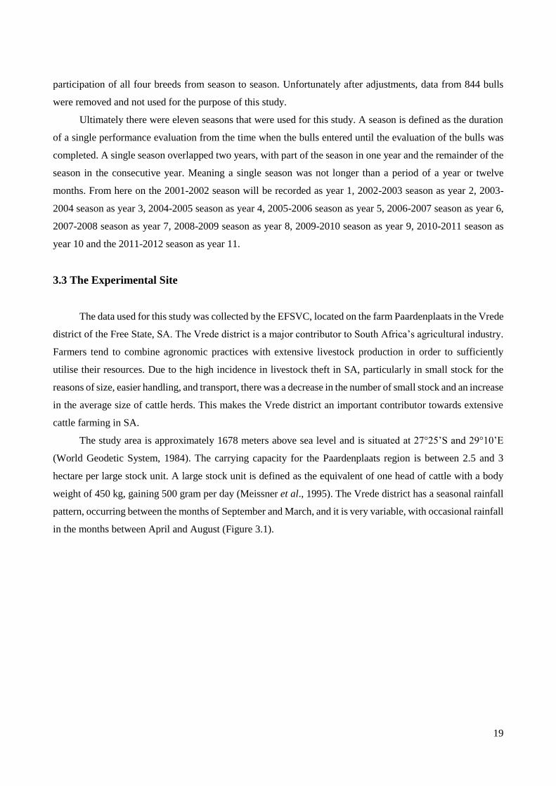


![ALCA - Beef Herds · 2016. 6. 16. · problems with low birthweight Red and Black [Angus] bulls. So about 5 years ago [2001] we tried to get 20 Lowline bulls, with great difficulty”,](https://static.documents.pub/doc/80x56/5fff40611159c655de2968c7/alca-beef-herds-2016-6-16-problems-with-low-birthweight-red-and-black-angus.jpg)

