EVALUATION OF RECURRENT NEURAL NETWORKS FOR CROP RECOGNITION FROM MULTITEMPORAL REMOTE SENSING IMAGES J. D. Bermúdez 1 , P. Achanccaray 1 , I. D. Sanches 3 , L. Cue 1 , P.Happ, 1 R. Q. Feitosa 1,2 1 Pontifical Catholic University of Rio de Janeiro, Brazil 2 Rio de Janeiro State University, Brazil 3 National Institute for Space Research, Brazil Comissão IV – Sensoriamento Remoto, Fotogrametria e Interpretação de Imagens ABSTRACT Agriculture monitoring is a key task for producers, governments and decision makers. The analysis of multitemporal remote sensing data allows a cost-effective way to perform this task, mainly due to the increasing availability of free satellite imagery. Recurrent Neural Networks (RNNs) have been successfully used in temporal modeling problems, representing the state-of-the-art in different fields. In this work, we compare three RNN variants: Simple RNN, Long- Short Term Memory (LSTM) and Gated Recurrent Unit (GRU), for crop mapping. We conducted a performance analysis of these RNN variants upon two datasets from tropical regions in Brazil using datasets from an optical (Landsat) and a SAR (Sentinel-1A) sensor. The results indicated that RNN techniques can be successfully applied for crop recognition and that GRU achieved slightly better performance than LSTM followed by Simple RNN. In terms of training time LSTM and GRU presented similar results, being approximately twice as slow as the simple RNN. Keywords: Crop Recognition, Deep Learning, Recurrent Neural Networks. 1- INTRODUCTION Agricultural mapping is essential for the design of policies aimed at food security. In this context, agricultural monitoring through sequences of multitemporal remote sensing images is a cost-effective solution compared to alternative approaches. The increasing availability of free satellite imagery with higher spatial resolutions and shorter revisit times allows capturing the evolution of crops throughout their phenological stages, estimating agricultural production with good accuracy. Among the different approaches proposed for crop mapping so far, those based on Probabilistic Graphical Models, like Markov Random Fields (Moser & Serpico, 2011) and Conditional Random Fields (Kenduiywo et al. 2017), and Deep Learning, such as Convolutional Neural Networks (Kussul et al. 2017), have attracted increasing attention due to their capacity to consider contextual information in spatial and/or temporal domains. These approaches achieve higher accuracies than conventional methods based on image stacking followed by classification via Support Vector Machines (SVM), Random Forest (RF), and Neural Networks (NN), among other classifiers. However, the computational effort associated to these methods, as well as their demand for labeled samples for adequate training are higher than conventional methods. Recurrent Neural Networks (RNNs) (Hopfield, 1982), in particular, Long-Short Term Memory networks (LSTMs) (Hochreiter & Schmidhuber, 1997) and their variants, have been successfully used in temporal modeling problems. RNNs were first proposed in the 1980s. However, their high computational cost, as well as difficulties to train them (vanish/explosion gradient problem) for long-term dependencies (Pascanu et al., 2013), made RNNs irrelevant for many years. Due to the growing computational power and the emergence of new network’s neural units architectures, RNNs have become a reference for many problems that involve sequence analysis. These networks represent the state-of-the-art in applications that include speech and text recognition (W. Xiong et al, 2017, Wenpeng et al, 2017). Despite similarities between such applications and crop recognition, there are few works in the literature using RNNs applied to the modeling of agricultural crop phenology. Exceptions are (You et al. 2017) and (Rußwurm & Körner, 2017), which use LSTM. This paper reports the results of an experimental comparison of three RNNs units architectures for crop recognition from sequences of multitemporal remote sensing images, specifically, a simple RNNs, LSTMs, and GRUs (Gated Recurrent Units). Two dataset were used: a Landsat 5/7 and a Sentinel-1 image sequences from the municipalities of Ipuã in São Paulo and Campo Verde in Mato Grosso state, respectively, both in Brazil. In the next section, we review fundamental concepts of RNNs and the LSTMs and GRUs neural 800 Sociedade Brasileira de Cartografia, Geodésia, Fotogrametria e Sensoriamento Remoto, Rio de Janeiro, Nov/2017 Anais do XXVII Congresso Brasileiro de Cartografia e XXVI Exposicarta 6 a 9 de novembro de 2017, SBC, Rio de Janeiro - RJ, p. 800-804 S B C
Transcript
EVALUATION OF RECURRENT NEURAL NETWORKS FOR CROP
RECOGNITION FROM MULTITEMPORAL REMOTE SENSING IMAGES
J. D. Bermúdez 1, P. Achanccaray 1, I. D. Sanches3, L. Cue1, P.Happ,1
R. Q. Feitosa 1,2
1Pontifical Catholic University of Rio de Janeiro, Brazil 2 Rio de Janeiro State University, Brazil
3 National Institute for Space Research, Brazil
Comissão IV – Sensoriamento Remoto, Fotogrametria e Interpretação de Imagens
ABSTRACT
Agriculture monitoring is a key task for producers, governments and decision makers. The analysis of multitemporal
remote sensing data allows a cost-effective way to perform this task, mainly due to the increasing availability of free
satellite imagery. Recurrent Neural Networks (RNNs) have been successfully used in temporal modeling problems,
representing the state-of-the-art in different fields. In this work, we compare three RNN variants: Simple RNN, Long-
Short Term Memory (LSTM) and Gated Recurrent Unit (GRU), for crop mapping. We conducted a performance
analysis of these RNN variants upon two datasets from tropical regions in Brazil using datasets from an optical
(Landsat) and a SAR (Sentinel-1A) sensor. The results indicated that RNN techniques can be successfully applied for
crop recognition and that GRU achieved slightly better performance than LSTM followed by Simple RNN. In terms of
training time LSTM and GRU presented similar results, being approximately twice as slow as the simple RNN.
Keywords: Crop Recognition, Deep Learning, Recurrent Neural Networks.
1- INTRODUCTION
Agricultural mapping is essential for the design
of policies aimed at food security. In this context,
agricultural monitoring through sequences of
multitemporal remote sensing images is a cost-effective
solution compared to alternative approaches. The
increasing availability of free satellite imagery with
higher spatial resolutions and shorter revisit times
allows capturing the evolution of crops throughout their
phenological stages, estimating agricultural production
with good accuracy.
Among the different approaches proposed for
crop mapping so far, those based on Probabilistic
Graphical Models, like Markov Random Fields (Moser
& Serpico, 2011) and Conditional Random Fields
(Kenduiywo et al. 2017), and Deep Learning, such as
Convolutional Neural Networks (Kussul et al. 2017),
have attracted increasing attention due to their capacity
to consider contextual information in spatial and/or
temporal domains. These approaches achieve higher
accuracies than conventional methods based on image
stacking followed by classification via Support Vector
Machines (SVM), Random Forest (RF), and Neural
Networks (NN), among other classifiers. However, the
computational effort associated to these methods, as
well as their demand for labeled samples for adequate
training are higher than conventional methods.
Recurrent Neural Networks (RNNs) (Hopfield,
1982), in particular, Long-Short Term Memory
networks (LSTMs) (Hochreiter & Schmidhuber, 1997)
and their variants, have been successfully used in
temporal modeling problems. RNNs were first proposed
in the 1980s. However, their high computational cost, as
well as difficulties to train them (vanish/explosion
gradient problem) for long-term dependencies (Pascanu
et al., 2013), made RNNs irrelevant for many years.
Due to the growing computational power and the
emergence of new network’s neural units architectures,
RNNs have become a reference for many problems that
involve sequence analysis. These networks represent the
state-of-the-art in applications that include speech and
text recognition (W. Xiong et al, 2017, Wenpeng et al,
2017). Despite similarities between such applications
and crop recognition, there are few works in the
literature using RNNs applied to the modeling of
agricultural crop phenology. Exceptions are (You et al.
2017) and (Rußwurm & Körner, 2017), which use
LSTM.
This paper reports the results of an
experimental comparison of three RNNs units
architectures for crop recognition from sequences of
multitemporal remote sensing images, specifically, a
simple RNNs, LSTMs, and GRUs (Gated Recurrent
Units). Two dataset were used: a Landsat 5/7 and a
Sentinel-1 image sequences from the municipalities of
Ipuã in São Paulo and Campo Verde in Mato Grosso
state, respectively, both in Brazil.
In the next section, we review fundamental
concepts of RNNs and the LSTMs and GRUs neural
800Sociedade Brasileira de Cartografia, Geodésia, Fotogrametria e Sensoriamento Remoto, Rio de Janeiro, Nov/2017
Anais do XXVII Congresso Brasileiro de Cartografia e XXVI Exposicarta 6 a 9 de novembro de 2017, SBC, Rio de Janeiro - RJ, p. 800-804S B
C
units network architectures. The following sections
describe the methods evaluated in this work for crop
recognition, the datasets used in our experiments, the
extracted features and the experimental protocol
followed in the experiments. Finally, we present and
discuss the results obtained in our experiments,
summarize the conclusions and indicate future works.
2- RECURRENT NEURAL NETWORKS (RNNs)
a) Fundamentals of RNNs
RNNs are a set of neural networks specialized
for processing sequential data. Basically, RNNs are
neural networks with feedback. The state of the network
at each point in time depends on both the current input
and the previous information stored in the network,
which allows the modeling of data sequences. This
capacity can be useful for modeling crop changes over
time.
A standard RNN architecture is shown in Fig
1. Given an input sequence (𝐱 = 𝒙0, 𝒙1, 𝒙3, . . , 𝒙𝑡−1, 𝒙𝑡),
the output of the network �̂� at each time index 𝑡 is given
by:
𝒉𝑡 = 𝑓(𝒃 + 𝑾𝒉𝑡−1 + 𝑼𝒙𝑡) (1)
�̂�𝑡 = 𝑔(𝒄 + 𝑽𝒉𝑡) (2)
where 𝒉𝑡 is the state of the network at time t, 𝒃 and 𝒄are bias weight vectors, 𝑾, 𝑼 and 𝑽 are weight matrices
and 𝑓 and 𝑔 are usually a tanh and softmax activation
functions, respectively. By applying Eq 1 and Eq 2
recursively for a sequence of length 𝜏, the graph can be
unfolded as shown in Fig 1 for 𝜏 = 3.
During training, a loss cost function 𝐿
quantifies the error between predicted and actual classes
at each time step. The total loss is computed by
summing the losses over all time steps. Then, the
networks parameters are adjusted via back-propagation
through time (BPTT) (Werbos, 1990) algorithm.
The RNN architecture shown in Fig 1 is also
known as “many to many” because it takes as input a
sequence of length 𝜏 and outcomes another sequence of
the same length. In some applications, it is about
labeling the whole sequence or predicting only the final
label of the sequence. The RNN architecture used for
this kind of problems is known as "many to one"
because it takes as input a sequence and predicts just
one value.
Two of the most widely used RNNs are
presented in the following.
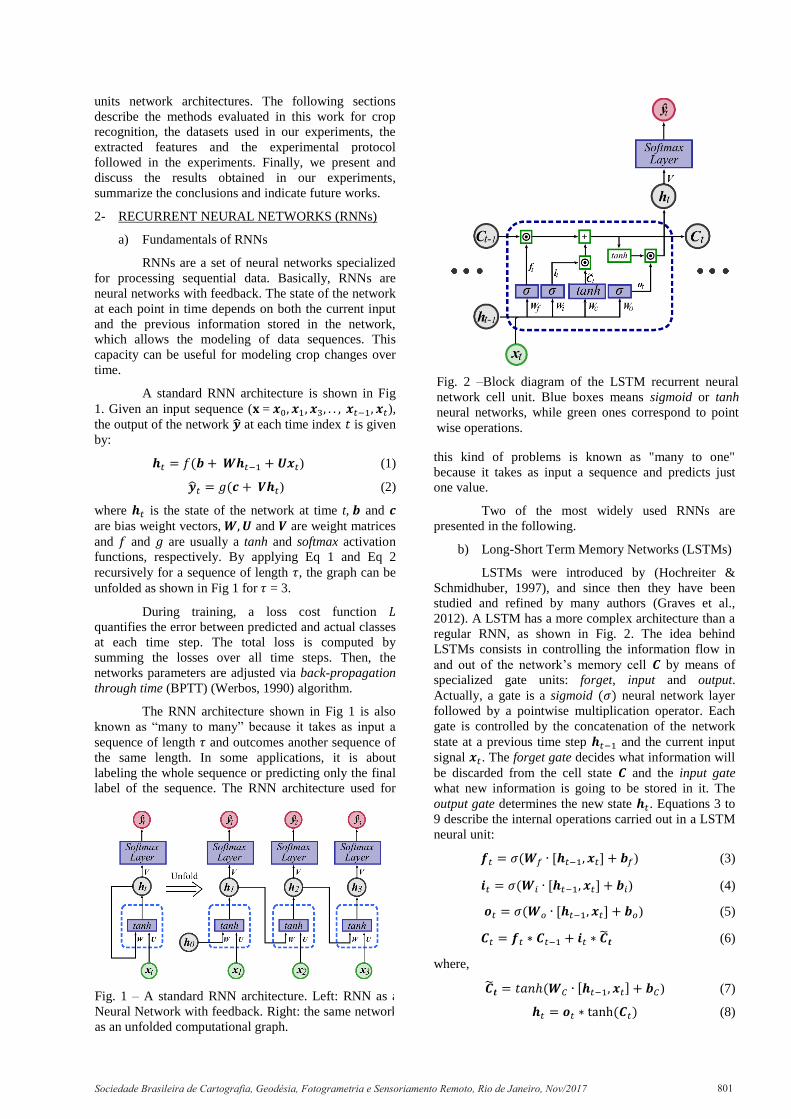
b) Long-Short Term Memory Networks (LSTMs)
LSTMs were introduced by (Hochreiter &
Schmidhuber, 1997), and since then they have been
studied and refined by many authors (Graves et al.,
2012). A LSTM has a more complex architecture than a
regular RNN, as shown in Fig. 2. The idea behind
LSTMs consists in controlling the information flow in
and out of the network’s memory cell 𝑪 by means of
specialized gate units: forget, input and output.
Actually, a gate is a sigmoid (𝜎) neural network layer
followed by a pointwise multiplication operator. Each
gate is controlled by the concatenation of the network
state at a previous time step 𝒉𝑡−1 and the current input
signal 𝒙𝑡. The forget gate decides what information will
be discarded from the cell state 𝑪 and the input gate
what new information is going to be stored in it. The
output gate determines the new state 𝒉𝑡. Equations 3 to
9 describe the internal operations carried out in a LSTM
neural unit:
𝒇𝑡 = 𝜎(𝑾𝑓 ∙ [𝒉𝑡−1, 𝒙𝑡] + 𝒃𝑓) (3)
𝒊𝑡 = 𝜎(𝑾𝑖 ∙ [𝒉𝑡−1, 𝒙𝑡] + 𝒃𝑖) (4)
𝒐𝑡 = 𝜎(𝑾𝑜 ∙ [𝒉𝑡−1, 𝒙𝑡] + 𝒃𝑜) (5)
𝑪𝑡 = 𝒇𝑡 ∗ 𝑪𝑡−1 + 𝒊𝑡 ∗ �̃�𝒕 (6)
where,
�̃�𝒕 = 𝑡𝑎𝑛ℎ (𝑾𝐶 ∙ [𝒉𝑡−1, 𝒙𝑡] + 𝒃𝐶) (7)
𝒉𝑡 = 𝒐𝑡 ∗ tanh (𝑪𝑡) (8)
Fig. 1 – A standard RNN architecture. Left: RNN as a
Neural Network with feedback. Right: the same network
as an unfolded computational graph.
Fig. 2 –Block diagram of the LSTM recurrent neural
network cell unit. Blue boxes means sigmoid or tanh
neural networks, while green ones correspond to point
wise operations.
801Sociedade Brasileira de Cartografia, Geodésia, Fotogrametria e Sensoriamento Remoto, Rio de Janeiro, Nov/2017
where 𝑾𝑓 , 𝑾𝑖, 𝑾𝑜, and 𝑾𝐶 and 𝒃𝑓 , 𝒃𝑖 , 𝒃𝑜 and 𝒃𝐶 are
weigth matrices and bias vectors, respectively, to be
learned by the network during training.
c) Gate Recurrent Unit (GRU)
A Gate Recurrent Unit (GRU) is a LSTM
variant with a simpler architecture, introduced in
(Chungetal, 2014). It has a reduced number of gates,
thus, there are fewer parameters to be tuned. Although a
GRU is simpler, its performance was similar to an
LSTM in many applications (Chungetal, 2014). As
shown in Fig. 3, the GRU neural unit architecture is
formed by two gates: update and reset. The update gate
𝒛𝑡 selects if the hidden state is to be updated with a new
hidden state 𝒉 ̂𝑡, while the reset gate 𝒓𝑡 decides if the
previous hidden state is to be ignored. See Eqs. (9-12)
for detailed equations of 𝒓𝑡, 𝒛𝑡, 𝒉𝑡 and 𝒉 ̂𝑡. Another
important difference with respect to LSTMs is that GRU
drops out the use of the cell memory 𝑪, so that the
memory of the network is only handled by the hidden
state 𝒉𝑡, resulting in less memory demand.
𝒛𝑡 = 𝜎(𝑾𝑧 ∙ [𝒉𝑡−1, 𝒙𝑡]) (9)
𝒓𝑡 = 𝜎(𝑾𝑟 ∙ [𝒉𝑡−1, 𝒙𝑡]) (10)
𝒉𝑡 = (1 − 𝒛𝑡) ∗ 𝒉𝑡−1 + 𝒛𝑡 + �̃�𝒕 (11)
where,
�̃�𝒕 = 𝑡𝑎𝑛ℎ (𝑾ℎ ∙ [𝒓𝑡 ∗ 𝒉𝑡−1, 𝒙𝑡]) (12)
where 𝑾𝑧 , 𝑾𝑟 , and 𝑾ℎ are the weigth matrices to be
learned by the network during training.
3- METHODOLOGY
The aforementioned RNN architectures were
evaluated in this work for crop recognition via pixel-
wise classification considering only the temporal
context. In our experiments, we classified only the last
epoch of the sequence, so we adopted the “many to one”
architecture, as is illustrated in Fig 4. Accordingly, each
input sequence 𝐱 is the set of features observed at each
site over time and the network's output �̂� is the
corresponding predicted label, given the input sequence
𝐱. In others words, at each time step t, the network is fed
with the extracted features 𝒙𝑡 of the site being analyzed.
Here, the RNN models the crop phenology over time by
considering at each time step observation in both the
previous and in the current epoch. During training, the
loss considering the predicted and actual class is
computed. Then, the networks’s internal parameters are
updated via the BPTT algorithm. Finally, the learned
model is evaluated in the sites not considered during
training.
4- EXPERIMENTS
a) Datasets
Two datasets from different sensors were
considered in this work:
Ipuã
It comprises a sequence of 9 co-registered
Landsat (5/7) images, taken between August 2000 and
July 2001, from the municipality of Ipuã in São Paulo
state, Brazil. Each image covers an extension of 465
km2, approximately with 30m spatial resolution. The
reference for each epoch was produced manually (visual
interpretation) by a human expert. The distribution of
classes per image is shown in Fig. 5. The main crops are
Sugarcane, Soybean and Maize. Other classes present in
the area are Pasture, Riparian Forest, Prepared Soil
(which corresponds to ploughing and soil grooming
phases), Postharvest (characterized by vegetation
residues lying on the ground) and Others that encloses
minor crops as well as rivers and urban areas.
i) Campo Verde
It comprises a sequences of 14 co-registered
Sentinel-1A images dual polarized (VH and VV), taken
between October 2015 and July 2016, from the
municipality of Campo Verde in Mato Grosso state,
Brazil. Each image covers an extension of 4782 km2
Fig. 4 – Many to One RNN architecture. The output
of the network �̂� is computed at the last time
observation.
Fig. 3 – Block diagram of the GRU recurrent neural
unit. Blue boxes means sigmoid or tanh neural
networks, while green ones correspond to point wisee
operations.
802Sociedade Brasileira de Cartografia, Geodésia, Fotogrametria e Sensoriamento Remoto, Rio de Janeiro, Nov/2017
Fig. 5 – Percentage of samples per class in Ipuã
dataset.
Fig. 6 – Percentage of samples per class in Campo
Verde dataset.
approximately with 10 m spatial resolution. There are
two images per month for November, December,
March, May and July and only one image for October,
January, February and June. The main crops found in
this area are Soybean, Maize and Cotton. Also, there are
some minor crops such as Beans and Sorghum. As non-
commercial crops (NCC), Millet, Brachiaria and
Crotalaria were considered. Other classes present in the
dataset are Pasture, Eucalyptus, Soil, Turf grass and
Cerrado. Fig. 6 shows the class occurrence per image in
the dataset.
b) Feature Extraction
For Ipuã dataset, the feature vector corresponds
to the pixel spectral data from bands 1-5 and 7, and the
Normalized Difference Vegetation Index (NDVI). For
Campo Verde dataset, we extracted Gray Level Co-
occurrence Matrix (GLCM) features. Similar to
(Kenduiywo et al., 2017), we computed for each image
band four features (correlation, homogeneity, mean and
variance) from the GLCM in four directions (0, 45, 90
and 135 degrees) using 3×3 windows. Therefore, each
pixel was represented by a feature vector of
dimensionality 32.
c) Experimental Protocol
We used the Keras framework (Chollet et al.,
2015) implementations in our experiments. A manual
parameter tuning was carried out for all experiments.
The dimension of state of the networks was set to 40
and the dropout regularization to 0.5.
The protocol followed in the experiments
basically consists of classifying only the image
corresponding to the last epoch in the sequence. For
Ipuã we considered the whole image sequence from
February to July. For Campo Verde we considered three
image sequences: the first one from November, 2014 to
February, 2015, where Soybean comes about, the
second one from March to July, where Cotton and
Maize are present, and the third one comprising the
whole sequence, which represents a more complex crop
dynamics due to the presence of crop rotation in some
sites. For Campo Verde we split the sites into five
mutually exclusive subsets, so as to have approximately
the same distributions of classes among all subsets. We
adopted a k-fold procedure so that at each fold one
subset was used for training and the remaining ones for
testing, i.e., approximately 20% for training and 80%
for testing at each fold. Experiments were run 10 times
per fold, for a total of 50 executions. For the Ipuã
dataset, we only considered one fold of 20% and 80%
approximately for training and testing, respectively and
executed the experiments 50 times. In this case, the
network weights initialization was the only random
factor that influenced the network outcomes.
In order to balance the number of training
samples for all classes we replicated the training
samples of less abundant classes in both datasets. For
Ipuã, 5,000 and for Campo Verde, 50,000 samples per
class were selected for the training set.
5- RESULTS
The Overall Accuracies (OA) obtained for Ipuã
are shown in Fig. 7. The boxplots show that LSTM and
GRU performed better than Simple RNN in approx.
3.5%. GRU outperformed LSTM just marginally in
terms of OA mean and variance.
Results for the three evaluated sequences of
Campo Verde dataset are shown in Fig 8. Unlike Ipuã,
all RNN architectures performed for Campo Verde
similarly. In fact, the boxplots exhibit high variance
values in all evaluated sequences. Recall that for
sequences 2 and 3, the same image was classified. The
performance for sequence 3 were better than for
sequence 2. This indicates that data not present in
sequence 2 from earlier epochs helped somehow to
improve the accuracy, even though the crop dynamics in
sequence 3 is more complex.
The differences between Campo Verde and
Ipuã results are due to at least two reasons. First, in the
803Sociedade Brasileira de Cartografia, Geodésia, Fotogrametria e Sensoriamento Remoto, Rio de Janeiro, Nov/2017
experiments on Ipuã, the training/testing set
configuration was kept constant in all experiment runs.
Second, the optical data is clearly more discriminative
than SAR data.
We also measured the average training times.
For sequence 1, whose processing time is similar to
sequence 2, Simple RNN took 162 seconds, GRU 343
seconds, and LSTM 364 seconds. For sequence 3, in the
same order, the execution time was 236, 408 and 432
seconds. For Ipuã dataset, the relative execution times
were approximately the same as for Campo Verde. As
for the computational efficiency, the simple RNN was
trained approximately twice as fast as GRU and LSTM.
In terms of accuracy, GRU was the best or nearly the
best among the tested architecture.
6- CONCLUSION
In this work, we compared the performance of
three different RNNs architectures, i.e., Simple RNN,
LSTM and GRU, for crop recognition in two
multitemporal remote sensing datasets, specifically from
Landsat and Sentinel 1A sensors. This study showed
that GRU and LSTM outperformed the Simple RNN for
a Landsat sequence. For the Sentinel-1A sequences all
evaluated networks performed similarly in terms of
accuracy. As for the computational load associated to
the training phase, GRU was consistently the most
efficient architecture.
Further studies include experiments in other
datasets and in other RNN configurations like “many to
many”, which allows the use of references in all epochs.
The addition of spatial contextual information is also
expected to improve results.
ACKNOWLEDGEMENTS
The authors acknowledge the funding provided
by CAPES and CNPq.
REFERENCES
Chung, J; C. Gulcehre; K. Cho and Y. Bengio, 2014,
Empirical evaluation of gated recurrent neural networks
on sequence modeling. arXiv preprint arXiv:1412.3555.
Graves, I, 2012. Supervised sequence labelling with
recurrent neural networks, Springer, Vol. 385.
Hochreiter, S. and J. Schmidhuber, 1997, Long short-
term memory, Neural computation, Vol.9, Nº8,
pp.1735–1780.
Hopfield, J, 1982, Neural networks and physical
systems with emergent collective computational
abilities’, Proceedings of the national academy of
sciences, Vol.79, Nº8, pp.2554–2558.
Kenduiywo, B. K; D. Bargiel and U. Soergel, 2017,
Higher order dynamic conditional random fields
ensemble for crop type classification in radar images,
IEEE Transactions on Geoscience and Remote Sensing.
Kussul, N; M. Lavreniuk; S. Skakun and A. Shelestov
2017, Deep learning classification of land cover and
crop types using remote sensing data, IEEE Geoscience
and Remote Sensing Letters, Vol.14, Nº5, pp.778–782.
Moser, G. and S. Serpico, 2011, Multitemporal region-
based classification of high-resolution images by
markov random fields and multiscale segmentation, in
Geoscience and Remote Sensing Symposium
(IGARSS), 2011 IEEE International, IEEE, pp. 102–
105.
Pascanu, R; T. Mikolov and Y. Bengio, 2013, On the
difficulty of training recurrent neural networks, in
International Conference on Machine Learning, pp.
1310–1318.
Rußwurm, M. and M. Körner, 2017, Multi-temporal
land cover classification with long short-term memory
neural networks, in International Archives of the
Photogrammetry, Remote Sensing & Spatial
Information Sciences 42.
Werbos, P. J, 1990, Backpropagation through time:
what it does and how to do it, in Proceedings of the
IEEE Vol.78, Nº10, pp.1550–1560.
You, J; X. Li; M. Low; D. Lobell and S. Ermon, 2017,
Deep gaussian process for crop yield prediction based
on remote sensing data, in AAAI, pp. 4559–4566.
Fig. 7 – Boxplots of OA metrics for Ipuã dataset.
Fig. 8 – Boxplots of OA metrics for Campo Verde
dataset.
804Sociedade Brasileira de Cartografia, Geodésia, Fotogrametria e Sensoriamento Remoto, Rio de Janeiro, Nov/2017