Evaluation of Selected Finite Difference Solutions to the ...

METreportNo. 08/2020

ISSN 2387-4201

Oceanography

Evaluation of Selected FiniteDifference Solutions to the

Shallow Water EquationsAlgorithms, Fortran code and examples

Lars Petter Røed

jj−1 j+1

k

k−1

k+1

∆y

∆x

METreport

Title Date

Evaluation of Selected Finite Difference Solutions to the

Shallow Water Equations

September 10, 2020

Section Report no.

Ocean and Ice 08/2020

Author Classification

Lars Petter Røed ③Free ❥Restricted

Client(s) Client’s reference

Research Council of Norway 250935/O70

Abstract

Considered are three different finite difference schemes to solve the rotating, two-dimensional shallow water equations.

These are the linear forward-backward scheme (FB-L), the linear centered in time, centered in space scheme (CTCS-L) and

a nonlinear version of the latter (CTCS-N). The resulting algorithms are programmed using the FORTRAN 95 programming

language, and compiled and run on a PC using the PC’s central processing unit (CPU). The schemes are tested for four

cases, the breaking of a dam on a wet domain, geostrophic adjustment, small Kelvin waves and large Kelvin waves. The

solutions are compared with results from identical cases derived by Holm et al. (2020), who in addition to the above schemes

also included two modern finite volume schemes. It is undescored that while this work make use of the computer’s CPU, Holm

et al. (2020) utilized the computer’s graphical processor unit (GPU). The latter necessitates the use of a GPU programming

language. It is therefore of interest to investigate whether the results derived here are equal to those of Holm et al. (2020).

For all cases the two linear schemes provide results nearly identical to the results derived by Holm et al. (2020) using their

linear scheme. In contrast the solutions provided by the nonlinear CTCS-N scheme differ radically from those derived by

Holm et al. (2020) for two of the cases, namely the breaking on a wet domain and the large Kelvin wave cases. Interestingly

the CTCS-N solution derived here is more in line with what one would expect in terms of the physics involved, and also more

in line with the solutions provided by the two finite volume schemes of Holm et al. (2020).

Keywords

Oceanography, Numerical Modeling, Shallow Water Equations

Disciplinary signature Responsible signature

Magne Simonsen Kai H. Christensen

Abstract

Considered are three different finite difference schemes to solve the rotating, two-dimensional

shallow water equations. These are the linear forward-backward scheme (FB-L), the lin-

ear centered in time, centered in space scheme (CTCS-L) and a nonlinear version of the

latter (CTCS-N). The resulting algorithms are programmed using the FORTRAN 95 pro-

gramming language, and compiled and run on a PC using the PC’s central processing unit

(CPU). The schemes are tested for four cases, the breaking of a dam on a wet domain,

geostrophic adjustment, small Kelvin waves and large Kelvin waves. The solutions are

compared with results from identical cases derived by Holm et al. (2020), who in addition

to the above schemes also included two modern finite volume schemes. It is undescored

that while this work make use of the computer’s CPU, Holm et al. (2020) utilized the

computer’s graphical processor unit (GPU). The latter necessitates the use of a GPU pro-

gramming language. It is therefore of interest to investigate whether the results derived

here are equal to those of Holm et al. (2020). For all cases the two linear schemes pro-

vide results nearly identical to the results derived by Holm et al. (2020) using their linear

scheme. In contrast the solutions provided by the nonlinear CTCS-N scheme differ radi-

cally from those derived by Holm et al. (2020) for two of the cases, namely the breaking

on a wet domain and the large Kelvin wave cases. Interestingly the CTCS-N solution

derived here is more in line with what one would expect in terms of the physics involved,

and also more in line with the solutions provided by the two finite volume schemes of

Holm et al. (2020).

Norwegian Meteorological Institute

Org.no 971274042

[email protected]

www.met.no / www.yr.no

Oslo

P.O. Box 43, Blindern

0313 Oslo, Norway

T. +47 22 96 30 00

Bergen

Allégaten 70

5007 Bergen, Norway

T. +47 55 23 66 00

Tromsø

P.O. Box 6314, Langnes

9293 Tromsø, Norway

T. +47 77 62 13 00


Org.no 971274042

[email protected]


Oslo


0313 Oslo, Norway

T. +47 22 96 30 00

Bergen

Allégaten 70

5007 Bergen, Norway

T. +47 55 23 66 00

Tromsø



T. +47 77 62 13 00


Org.no 971274042

[email protected]


Oslo


0313 Oslo, Norway

T. +47 22 96 30 00

Bergen

Allégaten 70

5007 Bergen, Norway

T. +47 55 23 66 00

Tromsø



T. +47 77 62 13 00

Contents

1 Introduction 6

2 Governing Equations 7

3 Boundary and initial conditions 9

3.1 Closed boundary conditions . . . . . . . . . . . . . . . . . . . . . . . 10

3.2 Open boundary conditions . . . . . . . . . . . . . . . . . . . . . . . . 10

4 Model ocean and grid configuration 11

5 Finite difference equations 14

5.1 The FB-L scheme . . . . . . . . . . . . . . . . . . . . . . . . . . . . . 15

5.2 The CTCS-L scheme . . . . . . . . . . . . . . . . . . . . . . . . . . . 16

5.3 The CTCS-N scheme . . . . . . . . . . . . . . . . . . . . . . . . . . . 17

6 Boundary conditions 19

6.1 Conditions at the northern and southern walls . . . . . . . . . . . . . 20

6.2 Conditions at the open western and eastern boundaries . . . . . . . 20

6.3 The Coriolis terms near closed boundaries . . . . . . . . . . . . . . 21

7 Cases studied 22

7.1 Case I: Dam break on a wet domain . . . . . . . . . . . . . . . . . . 22

7.2 Case II: Rossby adjustment . . . . . . . . . . . . . . . . . . . . . . . 25

7.3 Case III: Small Kelvin waves . . . . . . . . . . . . . . . . . . . . . . . 26

7.4 Case IV: Large Kelvin waves . . . . . . . . . . . . . . . . . . . . . . . 28

8 Results and discussions 29

8.1 Case I: Dam break on a wet domain . . . . . . . . . . . . . . . . . . 29

8.2 Cases II: Rossby adjustment . . . . . . . . . . . . . . . . . . . . . . . 32

8.3 Cases III: Small Kelvin waves . . . . . . . . . . . . . . . . . . . . . . 35

8.4 Cases IV: Large Kelvin waves . . . . . . . . . . . . . . . . . . . . . . 37

9 Summary and some final remarks 41

A The FORTRAN program 47

A.1 The main program nonlinear_swe.f90 . . . . . . . . . . . . . . . . . 47

4

A.2 Subroutine init.f90 . . . . . . . . . . . . . . . . . . . . . . . . . . . 72

A.3 Subroutine savef.f90 . . . . . . . . . . . . . . . . . . . . . . . . . . . 78

A.4 Subroutine store.f90 . . . . . . . . . . . . . . . . . . . . . . . . . . . 84

A.5 Subroutine ctcs-n.f90 . . . . . . . . . . . . . . . . . . . . . . . . . . 95

A.6 Subroutine euler-n.f90 . . . . . . . . . . . . . . . . . . . . . . . . . 102

A.7 Subroutine ctcs-l.f90 . . . . . . . . . . . . . . . . . . . . . . . . . . 109

A.8 Subroutine euler-l.f90 . . . . . . . . . . . . . . . . . . . . . . . . . 114

A.9 Subroutine fbl.f90 . . . . . . . . . . . . . . . . . . . . . . . . . . . . 119

5

1 Introduction

Considered are solutions to the rotating shallow water equations utilizing three different

numerical finite difference schemes. To this end four of the cases presented by Holm et al.

(2020) are revisited, namely

• Case I: Dam break on a wet domain,

• Case II: Rossby adjustment,

• Case III: Small Kelvin waves

• Case IV: Large Kelvin waves.

Case I corresponds to Case A of Holm et al. (2020), Case II to Case B and Cases III and

IV to the small and large Kelvin waves cases included in their Case D.

All solutions are derived on an Arakawa C-grid (Lattice C of Mesinger and Arakawa,

1976; Røed, 2019) using three somewhat different schemes. These are

• FB-L: the Forward-Backward Linear scheme,

• CTCS-L: the linear version of the traditional Centered in Time, Centered in Space

scheme (CTCS), also widely known as the leapfrog scheme,

• CTCS-N: the nonlinear version of the CTCS scheme

The FB-L scheme, which is identical to the linear scheme studied by Holm et al.

(2020), is credited to Sielecki (1968). It was for instance used by Martinsen et al. (1979)

in an early study of storm surges along the western coast of Norway. The nonlinear CTCS-

N scheme is the traditional choice for solving the shallow water equations on a rotating

frame on an Arakawa C-grid within the atmospheric and oceanographic communities.

Furthermore, it is commonly one of the options offered in Numerical Weather Prediction

(NWP) and Numerical Ocean Weather Predicition (NOWP) models. It is also identical to

the nonlinear scheme studied by Holm et al. (2020).

Since the cases and the two of the schemes (FB-L and CTCS-N) studied were also

investigated by Holm et al. (2020), the solutions derived using these two schemes are

compared to the solutions obtained by them. The CTCS-L scheme, which was not studied

by Holm et al. (2020), is added merely to check the linear solution derived using the FB-L

6

scheme. Interestingly Holm et al. (2020) also included two additional nonlinear schemes,

namely the KP scheme (credited to Kurganov and Petrova, 2007) and CDKLM scheme

(credited to Chertok et al., 2018). These are two more modern schemes developed, among

other things, to handle shocks. Hence they are expected to produce decent results even

for Cases I and IV which include shocks. It is underscored that while this study uses

the computer’s Central Processing Unit (CPU), Holm et al. (2020) uses the computer’s

Graphical Processing Unit (GPU). It is therefore of interest to compare the results derived

here with those of Holm et al. (2020).

Below Section 2 gives a brief introduction to the nonlinear and linear shallow water

equations followed by a brief outline of the continuum boundary conditions (Section 3).

Details about the model ocean design and grid configuration are revealed by Section 4.

Sections 5 provide details on the finite difference analogue of the governing equations

for each of the three numerical schemes, and the finite difference form of the boundary

conditions is treated in Section 6. Section 7 provides details about the four test cases,

while Section 8 presents and discusses the results. Finally Section 9 offers a summary and

some final remarks. An Appendix A is added to present the somewhat lenghty Fortran

program used to solve the governing equations.

2 Governing Equations

The non-linear, rotating shallow water equations written in flux form, which may be found

in almost any textbook on oceanography (e.g., Røed, 2019, eqs. 1.26 and 1.27 on page 7),

are

∂tU = − f k×U︸︷︷︸

Coriolis

−gh∇Hη︸︷︷︸

Pressure

−∇H ·(

UU

h

)

︸︷︷︸

Advective flux

+ X︸︷︷︸

Forcing

, (1)

∂th = − ∇H ·U︸︷︷︸

Divergence

, (2)

where

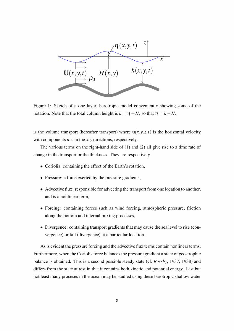
h(x,y, t) = η(x,y, t)+H(x,y), (3)

is the thickness of a water column, η being the deviation of the surface away from its equi-

librium depth H as illustrated in Figure 1, f is the Coriolis parameter, g denotes the the

gravitational acceleration, and X includes all external and internal forcing. Furthermore,

U =∫ η

−Hudz (4)

7

x

z

U(x,y, t) H(x,y) h(x,y, t)ρ0

η(x,y, t)

Figure 1: Sketch of a one layer, barotropic model conveniently showing some of the

notation. Note that the total column height is h = η +H, so that η = h−H.

is the volume transport (hereafter transport) where u(x,y,z, t) is the horizontal velocity

with components u,v in the x,y directions, respectively.

The various terms on the right-hand side of (1) and (2) all give rise to a time rate of

change in the transport or the thickness. They are respectively

• Coriolis: containing the effect of the Earth’s rotation,

• Pressure: a force exerted by the pressure gradients,

• Advective flux: responsible for advecting the transport from one location to another,

and is a nonlinear term,

• Forcing: containing forces such as wind forcing, atmospheric pressure, friction

along the bottom and internal mixing processes,

• Divergence: containing transport gradients that may cause the sea level to rise (con-

vergence) or fall (divergence) at a particular location.

As is evident the pressure forcing and the advective flux terms contain nonlinear terms.

Furthermore, when the Coriolis force balances the pressure gradient a state of geostrophic

balance is obtained. This is a second possible steady state (cf. Rossby, 1937, 1938) and

differs from the state at rest in that it contains both kinetic and potential energy. Last but

not least many proceses in the ocean may be studied using these barotropic shallow water

8

equations. Prime examples are tidal motion and storm surges1.

As mentioned the forcing term includes wind traction and atmospheric pressure forc-

ing in addition to mixing. It therefore takes the form

X = Ev +τs − τb

ρ0+∇H pa (5)

where Ev is the eddy viscosity (internal mixing term), τs is the winds stress due to the

wind’s traction on the surface, τb is the bottom stress due to friction at the bottom, and

∇H pa is the atmospheric pressure forcing. In contrast to the eddy viscosity the latter

three are all external forcing terms. They may therefore easily be added later. Henceforth

only mixing is included as a forcing term in what follows. The forcing term X therefore

reduces to

X = Ev. (6)

Since the governing equations are non-linear, the scheme may become numerically

unstable due to nonlinear instability (Phillips, 1959; Røed, 2019, chap. 10.3, page 217).

Here the mixing term comes in handy and may be used to squelch the nonlinear instability.

It then becomes an artificial or numerical mixing term. Commonly it is then parameter-

ized as a diffusive flux, that is,

Ev = ∇H ·F ; where F = A ·∇HU, (7)

where F is the eddy viscosity flux and A is the eddy viscosity (a tensor). Since the

mixing term is artificial, it is usually parameterized so that

A =

A 0 0

0 A 0

0 0 A

(8)

where A is a constant. Under these circumstances the eddy viscosity takes the final form

Ev = A∇2HU. (9)

3 Boundary and initial conditions

To solve (1) and (2) boundary and initial conditions are needed to determine the integra-

tion constants. Examination of (1) and (2) reveals that they are of second order in space.

1In many cases even the linear solution to the shallow water equations is a good approximation to

simulate tides and storm surges.

9

Thus eight boundary conditions are allowed, four in x and four in y. In time only three

initial conditions are allowed. If more are specified the system is overdetermined in a

mathematical sense, which may or may not lead to false solutions. Regarding the CTCS

schemes this leads to the well known initial boundary value problem as for instance ex-

plained by Røed (2019) (Chapter 5.6, page 84).

The conditions to be applied at the boundaries are either demanded by the physics of

the problem or, in the case of open boundaries, must be constructed (e.g., Chapman, 1985;

Røed and Cooper, 1987; Palma and Matano, 2000; Røed, 2019). In the cases detailed in

Section 7 the model ocean is contained within a rectangular basin oriented so that the

boundaries are aligned with the north-south and east-west directions. Furthermore, the

boundaries to the north and south are closed boundaries while the boundaries to the west

and east are open. Thus, both open and closed boundary conditions must be imposed.

3.1 Closed boundary conditions

At a closed boundary the transport components normal to and along the boundary is re-

quired to satisfy the so called no-slip condition. Hence

U = 0, at S, (10)

where S is the boundary. At the southern boundary of the domain, which is a straight,

coastal wall along y = 0, the no-slip condition takes the form

U =V = 0, at y = 0, ∀x. (11)

Likewise along the northern boundary y = Ly it takes the form

U =V = 0, at y = Ly, ∀x. (12)

3.2 Open boundary conditions

In Cases I and II the Flow Relaxation Scheme (FRS Røed, 2019, Chapter 7.5) is utilized

as an open boundary condition at the eastern and western boundaries. In contrast a cyclic

or periodic condition (Røed, 2019, Chapter 2.4, page 18) is applied in Cases III and IV.

A cyclic boundary condition is imposed by letting

U,V,h(x+Lx,y, t) =U,V,h(x,y, t). (13)

where Lx is the length of the basin in the eastern direction.

10

The FRS, which was originally developed by Davies (1976) for the atmosphere and

later adapted for ocean modeling by Engedahl (1995a), is a predictor-corrector scheme so

that

ψcorr = (1−α)ψpred +αψext . (14)

Here ψcorr is the corrector and ψpred is the predictor, while ψext is a specified external

solution. The coefficient α is such that 0 ≤ α ≤ 1 within the FRS zones at the eastern and

western end of the computational domain and zero elswhere. Thus, ψcorr =ψext at the end

of the computational domain and ψcorr = ψpred in the interior domain. In this respect it

is important that the gradient of α is as close to zero as possible at the boundary between

the FRS zone and the interior domain where α = 0. To achieve this the FRS zone has to

be sufficiently wide, say ∼10 grid points.

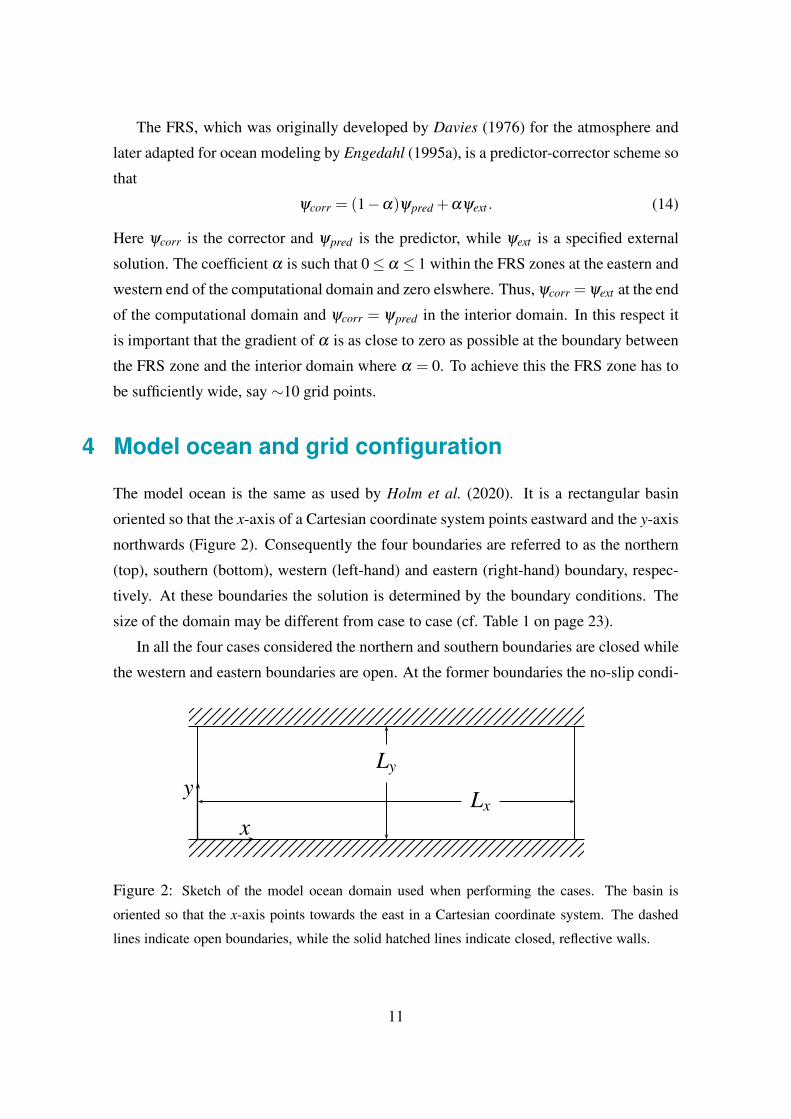
4 Model ocean and grid configuration

The model ocean is the same as used by Holm et al. (2020). It is a rectangular basin

oriented so that the x-axis of a Cartesian coordinate system points eastward and the y-axis

northwards (Figure 2). Consequently the four boundaries are referred to as the northern

(top), southern (bottom), western (left-hand) and eastern (right-hand) boundary, respec-

tively. At these boundaries the solution is determined by the boundary conditions. The

size of the domain may be different from case to case (cf. Table 1 on page 23).

In all the four cases considered the northern and southern boundaries are closed while

the western and eastern boundaries are open. At the former boundaries the no-slip condi-

x

yLx

Ly

Figure 2: Sketch of the model ocean domain used when performing the cases. The basin is

oriented so that the x-axis points towards the east in a Cartesian coordinate system. The dashed

lines indicate open boundaries, while the solid hatched lines indicate closed, reflective walls.

11

tion is imposed (Section 3.1). At the open boundaries either a cyclic boundary condition

(Cases III and IV) or the Flow Relaxation Scheme (Cases I and II) (Section 3.2) is im-

posed.

The grid configuration used to construct the finite difference approximation (FDA)

to (1) and (2) is as outlined by Figure 3. It corresponds to Lattice C of Mesinger and

Arakawa (1976). The solid blue lines conform with the boundaries of the model ocean

shown by Figure 2. As is evident the model ocean boundaries are aligned along the

auxiliary points so that it goes through U -points along the western and eastern boundaries

and through V -points along the southern and northern boundaries. Thus there are no

V -points along the western and eastern boundaries, and no U -points along the northern

and southern boundaries. An extra line of cells (referred to as ghost cells) outside of the

model ocean domain is therefore added along the northern boundary to satisfy the no-slip

boundary condition (11) at the northern wall.

The choice of a staggered C-grid is done to properly handle the boundary conditions.

The Cartesian coordinate system has its origo at the auxiliary point in grid cell (1,1) as

displayed by Figure 3. The staggering of the grid is such that a U -point is staggered

one half grid length along the x direction with respect to an h-point, while a V -point is

staggered one half grid length along the y direction with respect to an h-point. Relative to

this Cartesian coordinate system the notation x j, yk, Unjk,V

njk,h

njk entails

x j = ( j−1)∆x, yk = (k−1)∆y, (15)

hnjk = h

[

( j− 3

2)∆x,(k− 3

2)∆y, tn

]

, (16)

Unjk = U

[

( j−1)∆x,(k− 3

2)∆y, tn

]

, (17)

V njk = V

[

( j− 3

2)∆x,(k−1)∆y, tn

]

. (18)

where ∆x,∆y are the space increments along x,y, respectively, the subscripts j,k are coun-

ters and refer to the respective cells of the C-grid holding the individual U,V,h-points in

space (Figure 3). The superscript n refers to time level such that the time tn = n∆t where

∆t is the time step.

12

+

+

+

+

+

+

+

+

+

+

+

+

+

+

+

+

+

+

+

+

+

+

+

+

+

+

+

+

+

+

+

+

+

+

+

+

+

+

+

+

+

+

+

+

+

+

+

+

+

+

+

+

+

+

+

+

+

+

+

+

+

+

+

+

+

+

+

+

+

+

+

+

+

+

+

+

+

+

+

+

+

1 2 3 j−1 j j+1 J −1 J J +1

1

2

3

k−1

k

k+1

K −1

K

K +1

y

x

Figure 3: The staggered grid configuration used by the FB-L, CTCS-L and CTCS-N schemes

corresponding to the rectangular basin shown by Figure 2. The space increments of the grid are

∆x,∆y, while the dummy indices j,k counts the grid cells in the x and y directions, respectively.

Circles correspond to h, η and H-points, horizontal dashes to U -points and vertical dashes to

V -points. The points marked with red plus signs are auxiliary points. Origo in the Cartesian

coordinate system corresponds to the auxiliary point located at the lower left-hand corner in cell

number (1,1) where the southern and western boundaries intersects.

13

5 Finite difference equations

The finite difference approxomations of the three schemes listed in Section 1 may for

instance be found in Røed (2019) (Chapters 6 and 9). For reference purposes they are

nevertheless repeated here. The starting point is the governing equations (1) and (2) in

their scalar form, viz.,

∂tU = fV −gh∂xη −∂x

(U2

h

)

−∂y

(UV

h

)

+Xu, (19)

∂tV = − fU −gh∂yη −∂x

(UV

h

)

−∂y

(V 2

h

)

+Xv, (20)

∂th = −∂xU −∂yV, (21)

η = h−H, (22)

where Xu,Xv are the forcing terms along the x-axis and y-axis, respectively. In accord with

(9) they take the forms

Xu = A(∂ 2

x U +∂ 2y U), and Xv = A

(∂ 2

x V +∂ 2y V), (23)

respectively.

To arrive at the linear version of (19) through (22) the nonlinear, advective flux terms

are discarded. Furthermore, it is assumed that the sea level deviation is small compared to

the depth of a water column, so that η ≪H everywhere. Since the mixing terms are added

mainly to squelch the nonlinear instability they are superfluous as well. Furthermore, the

bottom is assumed to be flat so that H = H0 where H0 is a uniform equilibrium depth.

Thus, (19) through (22) take the forms

∂tU = fV − c20∂xη, (24)

∂tV = − fU − c20∂yη, (25)

∂th = −∂xU −∂yV, (26)

η = h−H0, (27)

where c0 =√

gH0 is the phase speed of linear, coastally trapped Kelvin waves (cf. Røed,

2019, Chapter 6.3). It should be emphasized that (24) through (27) are stricly speaking

only valid for linear problems and for problems where η ≪ H0 everywhere. Neverthe-

less, solved numerically in cases when these approximations are violated, they may still

provide numerically stable solutions that may even look reasonable albeit being wrong.

14

5.1 The FB-L scheme

By replacing all the derivatives appearing in (24) through (27) by FDAs, and in doing so

employing the forward-backward scheme (Røed, 2019, Chapter 6) on the Arakawa C-grid

displayed by Figure 3), their finite difference versions become

hn+1jk = hn

jk +∆t

(

[Du]njk +[Dv]

njk

)

(28)

Un+1jk = Un

jk +∆t

(

[Cu]njk +[Pu]

n+1jk

)

, (29)

V n+1jk = V n

jk +∆t

(

[Cv]n+1jk +[Pv]

n+1jk

)

, (30)

ηn+1jk = hn+1

jk −H0, (31)

where

[Cu]njk =

1

4f

(

V njk−1 +V n

jk +V nj+1k +V n

j+1k−1

)

, (32)

[Cv]njk = −1

4f(

Unj−1k +Un

j−1k+1 +Unjk+1 +Un

jk

)

, (33)

are the Coriolis terms,

[Pu]njk = − c2

0

∆x

(

ηnj+1k −ηn

jk

)

, (34)

[Pv]njk = − c2

0

∆y

(

ηnjk+1 −ηn

jk

)

, (35)

are the pressure forcing terms, and

[Du]njk =− 1

∆x

(

Unjk −Un

j−1k

)

, [Dv]njk =− 1

∆y

(

V njk −V n

jk−1

)

(36)

are the divergence terms. Regarding the time levels notice that the pressure term in (29)

is evaluated at the new time level, and so is the pressure and Coriolis terms in (30). This

is why the scheme is referred to as a forward-backward scheme. The idea behind the

FB-L scheme is that as soon as one of the variables are updated to the new time level its

value is immediately used in the next equation. This is allowed since the scheme is linear.

The FB-L scheme is therefore a so called two time level scheme, which implies that only

two time levels have to be stored in memory at any time. The advantage of the two level

scheme is that it avoids the initial value problem.

As visualized by (32) and (33) the staggering of the Arakawa C-grid makes the eval-

uation of the Coriolis terms a bit awkward. Recall that in (29) the Coriolis term requires

V in cell ( j,k) to evaluated at a U -point, while in (30) it requires U to be evaluated at a

15

V -point. To arrive at the finite difference equations displayed by (32) and (33) an inter-

polation using the four nearest points in space is therefore employed. This interpolation

may have implications though regarding the implementation of the boundary condition at

closed boundaries (reflective walls) as described by Jamart and Ozer (1986) and detailed

in Section 6.3 below. Finally, it should be emphasized that in order to be numerically

stable the FB-L scheme requires that the CFL criteria

∆t <∆x

c0

√2

[

1+

(∆x

∆y

)2]− 1

2

(37)

is satisfied at all times.

5.2 The CTCS-L scheme

Like the FB-L scheme the CTCS-L scheme is a finite difference version of the linear

governing equations, that is, (24) through (27), and reads

Un+1jk = Un−1

jk +2∆t

(

[Cu]njk +[Pu]

njk

)

, (38)

V n+1jk = V n−1

jk +2∆t(

[Cv]njk +[Pv]

njk

)

, (39)

hn+1jk = hn−1

jk +2∆t

(

[Du]njk +[Dv]

njk

)

, (40)

ηn+1jk = hn+1

jk −H0 (41)

where the Coriolis terms [Cu]njk and [Cv]

njk, the pressure forcing terms [Pu]

njk and [Pv]

njk,

and the divergence terms [Du]njk and [Dv]

njk are as given by (32) through (36), respectively.

Inspection of the above equations reveals that the CTCS-L scheme is indeed a centered

in time, centered in space scheme, and in contrast to the FB-L scheme it is a three level

scheme. There are a few important changes to note. Due to the centering in time the

factor ∆t is replaced by 2∆t, and all terms on the right-hand side of (38) through (40) are

evaluated at time level n. It is therefore a true explicit scheme.

In addition, as outlined in Røed (2019) (Chapter 6.4), the CFL criterion for stability is

slightly more stringent than the criteria given by (37) regarding the FB-L scheme.

Like the FB-L scheme the CTCS-L scheme is afflicted by several disadvantageous

properties. Being a three time level scheme the CTCS-L scheme is troubled by the so

called initial value problem. In addition it contains numerical or artificial dispersion and

has a false computational mode (Røed, 2019).

16

Regarding the artificial dispersion the numerical dispersion relation for the CTCS-L

scheme in one dimension (Røed, 2019, Chapter 6.4, page 130) reads

c1,2(α) =± 1

α∆tarcsin

c0∆t

∆xsin(α∆x)

√

1+

(∆x

Lr sin(α∆x)

)2

, (42)

where α is the wavenumber, Lr = c0/ f is Rossby’s deforamtion radius, and c1,2 is the

numerical phase speed. The numerical phase speed is therefore a function of the wave-

length. If α∆x is large that particular wavelength is not well resolved, and the numerical

phase speed becomes significantly smaller than the true phase speed. Consequently, the

classic sign of numerical dispersion is a trail of waves of various wavelengths, usually

shorter than 4∆x, lagging behind the main distribution.

The initial problem is common to all centered in time schemes (Røed, 2019, page 84,

Chapter 5.6). It arises since knowledge of the variables at time t−1 is required when solv-

ing for the first time level n = 1. Since the governing equations only allow specification

of three initial conditions, the specification of the variables at both t = t0 and t = t−1 is

not allowed. The common remedy is to switch to a forward in time, centered in space

scheme (FTCS) to perform the first integration step in time. The simplest FTCS scheme

to employ is the Euler scheme. To arrive at at an Euler scheme the superscipts n−1 ap-

pearing on the right-hand side of (38), (39) and (40) are replaced by n and the factor 2∆t

on the right-hand side is replaced by ∆t. By doing so the Euler scheme reads

Un+1jk = Un

jk +∆t

(

[Cu]njk +[Pu]

njk

)

, (43)

V n+1jk = V n

jk +∆t(

[Cv]njk +[Pv]

njk

)

, (44)

hn+1jk = hn

jk +∆t

(

[Du]njk +[Dv]

njk

)

, (45)

ηn+1jk = hn+1

jk −H0. (46)

Finally keep in mind that the Euler scheme is unconditionally unstable. Nevertheless

to employ the Euler scheme once does not ruin the stability. Moreover, it may be done

from time to time to rule out the computational mode inherent in all CTCS schemes (cf.

Røed, 2019, Chapter 5.8).

5.3 The CTCS-N scheme

To solve the fully, nonlinear governing equation (19) through (22) a second order, centered

in time centered in space scheme is employed. Due to the inclusion of the nonlinear terms

17

the CTCS-N scheme is susceptible to nonlinear instabilities. An artificial eddy viscosity

term is therefore added to suppress these instabilities if needed (cf. Røed, 2019, Chapter

10.3).

Again the same Arakawa C-grid (Figure 3) is employed. The finite difference version

of (19) through (22) then take the forms

Un+1jk =

{

Un−1jk +2∆t

(

[Cu]njk +[Pu]

njk +[Ax

u]njk +[Ay

u]njk +[Mu]

njk

)}

R, (47)

V n+1jk =

{

V n−1jk +2∆t

(

[Cv]njk +[Pv]

njk +[Ax

v]njk +[Ay

v]njk +[Mv]

njk

)}

R, (48)

hn+1jk = hn−1

jk +2∆t(

[Du]njk +[Dv]

njk

)

, (49)

ηn+1jk = hn+1

jk −H jk (50)

where the factor

R =1

1+2A∆t(

1∆x2 +

1∆y2

) (51)

appears due to the application of the Dufort-Frankel FDA of the eddy viscosity (mixing)

terms. Since the Coriolis terms [Cu]njk and [Cv]

njk and the divergence terms [Du]

njk and

[Dv]njk are linear terms they are as listed by (32), (33) and (36), respectively. The pressure

terms, however, are nonlinear and now take the forms

[Pu]njk = − g

2∆x

(

hnj+1k +hn

jk

)(

ηnj+1k −ηn

jk

)

, (52)

[Pv]njk = − g

2∆y

(

hnjk+1 +hn

jk

)(

ηnjk+1 −ηn

jk

)

. (53)

In addition the nonlinear momentum flux terms and mixing terms are added. The former

take the finite difference forms

[Axu]

njk =− 1

4∆x

(

Unj+1k +Un

jk

)2

hnj+1k

−

(

Unjk +Un

j−1k

)2

hnjk

, (54)

[Ayu]

njk =− 1

∆y

(

Unjk+1 +Un

jk

)(

V nj+1k +V n

jk

)

hnjk +hn

jk+1 +hnj+1k+1 +hn

j+1k

−

(

Unjk +Un

jk−1

)(

V nj+1k−1 +V n

jk−1

)

hnjk−1 +hn

jk +hnj+1k +hn

j+1k−1

.

(55)

[Axv]

njk =− 1

∆x

(

Unjk+1 +Un

jk

)(

V nj+1k +V n

jk

)

hnjk +hn

jk+1 +hnj+1k+1 +hn

j+1k

−

(

Unj−1k+1 +Un

j−1k

)(

V njk +V n

j−1k

)

hnj−1k +hn

j−1k+1 +hnjk+1 +hn

jk

,

(56)

18

and

[Ayv]

njk =− 1

4∆y

(

V njk+1 +V n

jk

)2

hnjk+1

−

(

V njk +V n

jk−1

)2

hnjk

, (57)

respectively, while the mixing terms take the forms

[Mu]njk =

A

∆x2

(

Unj+1k −Un−1

jk +Unj−1k

)

+A

∆y2

(

Unjk+1 −Un−1

jk +Unjk−1

)

, (58)

and

[Mv]njk =

A

∆x2

(

V nj+1k −V n−1

jk +V nj−1k

)

+A

∆y2

(

V njk+1 −V n−1

jk +V njk−1

)

. (59)

Just like the CTCS-L scheme an Euler scheme has to be employed to start the integra-

tion. Thus, the superscipt n−1 appearing in the first terms on the right-hand sides of (47),

(48) and (49) is replaced by n, and the factor 2∆t by ∆t. In addition the Dufort-Frankel

FDA used for the mixing terms is abandoned and replaced by an ordinary second order

FDA. By doing so the Euler scheme takes the form

Un+1jk = Un

jk +∆t

(

[Cu]njk +[Pu]

njk +[Ax

u]njk +[Ay

u]njk +[M∗

u ]njk

)

, (60)

V n+1jk = V n

jk +∆t

(

[Cv]njk +[Pv]

njk +[Ax

v]njk +[Ay

v]njk +[M∗

v ]njk

)

, (61)

hn+1jk = hn

jk +∆t(

[Du]njk +[Dv]

njk

)

, (62)

ηn+1jk = hn+1

jk −H jk. (63)

where

[M∗u ]

njk =

A

∆x2

(

Unj+1k −2Un

jk +Unj−1k

)

+A

∆y2

(

Unjk+1 −2Un

jk +Unjk−1

)

, (64)

and

[M∗u ]

njk =

A

∆x2

(

V nj+1k −2V n

jk +V nj−1k

)

+A

∆y2

(

V njk+1 −2V n

jk +V njk−1

)

. (65)

It is emphasized that interpolation is used to arrive at the various FDAs listed above.

Thus some of the interpolations must be rewritten close to solid, reflective walls. In

particular this is true regarding the Coriolis terms (cf. Section 6.3 below).

6 Boundary conditions

6.1 Conditions at the northern and southern walls

19

Along the southern and northern boundaries the no-slip condition (11) and (12) requires

U as well as V to be zero there. Since the auxiliary points are on the boundary the FDA

of (11) and (12) read

U+nj1 =V n

j1 = 0, and U+njK =V n

jK+1 = 0 ; j = 2(1)J−1, ∀n, (66)

respectively. As before the notation U+nj1 and U+n

jK entails evaluation of U at an auxil-

iary point in the cells ( j,1) and ( j,K), respectively. Performing the interpolation U+njk =

12

(

Unjk +Un

jk+1

)

(66) takes the final form

Unj1 =−Un

j2, and V nj1 = 0 ; j = 2(1)J−1, ∀n, (67)

and

UnjK+1 =−Un

jK, and V njK+1 = 0 ; j = 2(1)J−1, ∀n. (68)

The closed boundary condition is therefore fulfilled by letting the values of the U -points

just outside the wall being mirrored across the model ocean boundary along the northern

and western boundaries. This explains why ghost cells have to be added outside of the

northern boundary.

6.2 Conditions at the open western and eastern boundaries

Along the eastern and western boundaries either the cyclic boundary condition or the FRS

is imposed. At open boundaries the governing equations are still valid. Thus, first U , V

and h are computed at the eastern boundary j = J + 1 using the schemes above. While

doing this any references to j = J + 2 must be replaced by j = 2 to satisfy the cyclic

boundary condition. Next, the cyclic boundary condition (13) requires that the solutions

at the western boundary j = 1 are updated according to

Un1k =Un

J+1k, V n1k =V n

J+1k and hn1k = hn

J+1k (69)

for k = 1(1)K+1 and for all n.

When using the FRS as the open boundary condition the Ng points closest to western

and eastern boundaries are first set aside to cover so called FRS zones, the remaining

points being referred to as interior points (cf. Røed, 2019, Figure 7.4, on page 172). Here

Ng must be a number larger than or equal to 7 (Engedahl, 1995a). Within the FRS zones

the solutions are relaxed towards specified solutions at the western and eastern boundaries.

The resulting solutions are therefore only valid within the interior domain. The FRS works

20

as a predictor-corrector scheme. In the first step, the predictor step, the integration of the

numerical scheme is performed as usual, but excludes the western and eastern boundary

points (the cells j = 1 and j = J +1). Letting the variables be represented by the vector

Y = [U,V,h,η]T the first step is performed by computing it from the numerical scheme

in question. For instance regarding the FB-L scheme it would read

Y∗jk = Yn

jk +L [Ynjk]; j = 2(1)J,k = 2(1)K. (70)

while for the CTCS-L and CTS-N it would read

Y∗jk = Yn−1

jk +L [Ynjk]; j = 2(1)J,k = 2(1)K. (71)

where L is an operator operating on Ynjk in accord with the chosen scheme and Y∗

jk is

the predictor. The next step, the corrector step, is performed by correcting the predictor

solution by relaxing it towards an exterior solution, that is,

Yn+1jk = (1−α j)Y

∗jk +α jY

ejk; j = 2(1)J,k = 2(1)K, (72)

Yn+11k = Ye

1k and Yn+1J+1k = Ye

J+1k; k = 2(1)K (73)

Here Yejk is the external solution, while α j is a relaxation parameter defined by

α j =

1− tanh(

j−13

)

if 1 < j < Ng,

0 if Ng ≤ j ≤ J+1−Ng,

1− tanh(

J+1− j3

)

if J+1−Ng < j < J +1.

(74)

It should be emphasized that this definition requires that Ng is sufficiently large so that

α is approaching one at the exterior end of the FRS zones, e.g., for j = 1, and that its

gradient is close to zero at the interior end of the FRS zones, e.g., j = Ng.

6.3 The Coriolis terms near closed boundaries

Since all schemes employ the same staggered C-grid, the Coriolis terms are the same for

all three schemes. Near closed boundaries, such as the northern and southern boundaries,

the interpolation due to the staggered C-grid uses values at points where V njk = 0 due to

the boundary condition. For instance close to the southern boundary at k = 2 (32) reads

[Cu]nj2 =

1

4f(V n

j1 +V nj2 +V n

j+12 +V nj+11

); j = 2(1)J. (75)

21

Here V nj1 and V n

j+11 are located at the southern boundary, and hence vanishes in accord

with (66). If the factor 14

in front of (75) is kept then, as shown by Jamart and Ozer

(1986), artificial boundary currents will appear. By replacing the factor 14

in (75) with 12

they showed that the boundary currents disappeared, and concluded that they were a true

numerical artifact. The same is true when considering the points closest to the northern

boundary (k = K).

Consequently the Coriolis term in (32) is multiplied by a function defined by

δk = f

14

if k = 3(1)K−1

12

if k = 2 or k = K. (76)

to read

[Cu]njk = δk

(

V njk−1 +V n

jk +V nj+1k +V n

j+1k−1

)

; j = 2(1)J, k = 2(1)K. (77)

7 Cases studied

As alluded to in the introduction (Section 1) four cases are considered. They are identical

to cases presented by Holm et al. (2020), which were constructed to test the ability of

the schemes presented in Section 5 to replicate a shock (Case I), adjustment under gravity

(Case II), and the advection of small and large amplitude Kelvin waves (Cases III and IV).

The salient numbers such as length and width of the model ocean domain, mesh sizes,

etc, are listed in Table 1. Details regarding the respective cases are given by Sections 7.1

through 7.4 below. Note that in accord with (15)

Lx = J∆x, and Ly = (K −1)∆y, (78)

where Lx,Ly are the physical dimensions of the model ocean domain in the east-west and

north-south direction, respectively (Figure 2). Thus Lx,J,∆x are interdependent and so

are Ly,K,∆y. Hence given two of them the third must be computed from (78).

7.1 Case I: Dam break on a wet domain

Corresponds to Case A of Holm et al. (2020). It has no rotation and is therefore a one-

dimensional problem. It is the traditional and commonly used test case of non-rotating

fluid dynamics to test a scheme’s ability to represent shocks. It is initiated as a state

of rest (U = V = 0) at time t = 0 (n = 0), but features an initial (small) step in the sea

22

Table 1: Symbols and values of parameters used to initialize the variables and to run the four

test cases. Lx,Ly are the dimensions of the model ocean domain in the east-west and north-south

direction, respectively (Figure 2). H0 is the equilibrium depth of the model ocean, f is the Coriolis

parameter, g is the gravitational acceleration, η0 is the amplitude, or maximum, of the initial sea

surface deviation, and x0 and y0 correspond to its location in the Cartesian coordinate system

(Figure 3). Furthermore, J + 1,K + 1 are the number of cells in the x,y directions, respectively,

while ∆x,∆y are the space increments in those directions, ∆t is the time step, and A is the eddy

viscosity coeffecient for the CTCS-N scheme only. Finally, N f l denotes the number of time steps

necessary for a linear Kelvin wave to propagate across the model domain in the east-west direction

once, and hence is applicable to Cases III and IV only.

Symbol Case I Case II Case III Case IV Unit

Lx 10−2 40000 5000 5000 km

Ly 10−3 50000 2000 2000 km

H0 0.005 1000 100 100 m

f 0 1.2 ·10−4 1.2 ·10−4 1.2 ·10−4 s−1

g 9.81 9.81 9.81 9.81 ms−2

η0 0.002 0.2 0.05 2.0 m

x0 5 ·10−3 20000 2500 2500 km

y0 - 25000 −5 −5 km

J+1,K +1 500/51 800,1001 1000,201 1000,201 -

∆x,∆y 2 ·10−5 50 5,10 5,10 km

∆t 0.01 100 Lx

N f l

√gH0

≈ 31.93 Lx

N f l

√gH0

≈ 31.93 s

A 0.1 25 25 25 m2s−1

N f l - - 5000 5000 -

surface deviation in middle of the domain which is then released (Figure 4). At the open

boundaries at the western and eastern end of the domain the FRS is imposed as the open

boundary condition (Section 6).

The initial sea surface deviation is such that it has a positive step westward with a

23

3 4 5 6 7x [m]

-0.003

-0.002

-0.001

0

0.001

0.002

0.003

Sea

surfa

ce d

evia

tion

[m]

Case I: Initial sea surface deviation

a)

b)

Figure 4: Case I: The initial sea surface deviation η in meters. Distances are in meters. Distance

in the east-west direction is truncated. a) Top view, and b) side view.

similar negative step eastward. Thus,

η(x,y,0) = η0

+1 if 0 < x ≤ x0,

0 if x = x0,

−1 if x0 < x ≤ Lx,

and U(x,y,0) =V (x,y,0) = 0. (79)

Here η0 is the the amplitude of the step and x0 = Lx/2 denotes the location halfway

between the western and eastern boundaries (Table 1).

The FDA of (79) is

η0jk = η0

+1 if 0 ≤ j ≤ j0,

−1 if j0 < j ≤ J +1,and U0

jk =V 0jk = 0. (80)

where j0 is the cell number where the location of the auxiliary point equals x0. Recall that

origo is at the auxilary point in cell (1,1) (Figure 3). Thus, j0 = 1+ Lx

2∆x, where ∆x is the

space increment and Lx the length of the model ocean domain in the east-west direction

(Table 1 for actual values). The initial condition for the sea surface deviation is therefore

as displayed by Figure 4.

24

7.2 Case II: Rossby adjustment

Corresponds to Case B of Holm et al. (2020). It is performed on a rotating earth. The

initial state is unbalanced so that U = V = 0 (zero transport), while the sea surface has

a smooth hump in the middle of the domain (Figure 5). This is the traditional test case

used in geophysical fluid dynamics to test a scheme’s ability to replicate the steady state

solution of geostrophic balance as time goes to infinity. Analytic solutions to this problem

with an initial step function was already derived by C. G. Rossby in the 1930s (Rossby,

1937, 1938). The FRS is imposed as the open boundary condition at the western and

eastern boundaries.

10000 12000 14000 16000 18000 20000 22000 24000 26000 28000 30000x [km]

-0.05

0

0.05

0.1

0.15

0.2

Se

a s

urf

ac

e d

ev

iati

on

[m

]

Case II: Initial state

a)

b)

Figure 5: Case II: The initial sea surface deviation in meters. a) Top view. Numbers along axes

are distance (unit is km, truncated in both direction). b) Side view is a cut along y = y0. Numbers

along the horizontal axis are distance (unit km) in the eastern direction (also truncated). The

vertical axis indicates sea surface deviation (unit m).

The sea surface deviation is given in accord with the formula of Holm et al. (2020)

25

(their Section 4.2), that is,

η(x,y,0) =1

2η0

[

1+ tanh

(

−√

(x− x0)2 +(y− y0)2 +D

L

)]

. (81)

Here D = 50∆x relates to the width of the hump, while L = 15∆x relates to its steepness.

Other values are give by Table 1.

With reference to Figure 3 the numerical rendition of the initial conditions take the

forms

U0jk =V 0

jk = 0, (82)

and

η0jk =

1

2η0

[

1+ tanh

(

−√

(x j −0.5∆x− x0)2 +(yk −0.5∆y− y0)2 +D

L

)]

, (83)

for all j = 1(1)J and k = 1(1)K, respectively. The initial two-dimensional hump is visu-

alized by Figure 5.

7.3 Case III: Small Kelvin waves

Corresponds to Case D of Holm et al. (2020), and is also very similar to Case IV (Section

7.4). In both cases the initial state consists of a wave trapped at the southern boundary

and travelling eastwards. The wave has its maximum at the southern boundary and decays

exponentially towards the northern boundary (Figure 6). It is a balanced state so that the

initial pressure gradient caused by the specified sea surface deviation is balanced by the

Coriolis force. Consequently U 6= 0 while V = 0.

Case III and Case IV test a scheme’s ability to properly represent Kelvin waves, which

are ubiqutous in the ocean. The only difference between the two cases is the initial max-

imum amplitude of the Kelvin wave. In Case III it is η0 = 0.05 m, while in Case IV it

is raised by a factor of 40 to η0 = 2 m. Accordingly, the response regarding Case III is

expected to be linear, while the response for Case IV is expected to be highly nonlinear.

Both cases make use of a cyclic boundary condition at the eastern and western boundaries.

In accord with Holm et al. (2020) the initial sea surface deviation takes the form

η(x,y,0) =1

2η0 exp

(

−√

(y− y0)2

Lr

)[

1+ tanh

(

−√

(x− x0)2 +Lr

Lr/3

)]

, (84)

26

1500 1750 2000 2250 2500 2750 3000 3250 3500x [km]

0

0.02

0.04

0.06

Sea s

urf

ace d

evia

tio

n [

m]

Case III: Initial state

a)

b)

Figure 6: Case III: The initial sea surface deviation in meters. a) Top view. Numbers along axes

are distance (unit km) in the eastern (horizontal) and northern (vertical) direction, respectively.

The distance in the eastern direction is truncated. b) Side view. The cut is along y = 0.5∆y.

Numbers along horizontal axis as in Panel a. Sea surface deviation (unit m) is indicated along the

vertical axis.

while the transport in the eastern direction is

U(x,y,0) = c0 sgn(y− y0)η(x,y,0) and V (x,y,0) = 0. (85)

In (84) and (85) c0 =√

gH0 is the phase speed of linear Kelvin waves and Lr = c0/ f is

Rossby’s deformation radius. Details regarding the other parameters are given by Table

1.

The numerical rendition of (84) is simply

η0jk =

1

2η0 exp

(

−√

(yk −0.5∆y− y0)2

Lr

)[

1+ tanh

(

−√

(x j −0.5∆x− x0)2 +Lr

Lr/3

)]

.

(86)

for all j = 1(1)J and k = 1(1)K. Recalling that U -points are staggered one half space

27

increment relative to the η-points the numerical rendition of (85) is

U0jk =

1

2c0 sgn(yk −0.5∆y− y0)

(

η0j+1k +η0

jk

)

and V 0jk = 0, (87)

again for all j = 1(1)J and k = 1(1)K.

7.4 Case IV: Large Kelvin waves

As shown by Figure 7 Case IV is similar to Case III, the only difference being that the

initial maximum amplitude of the hump is raised 40 times to η0 = 2 m (Table 1).

1500 1750 2000 2250 2500 2750 3000 3250 3500x [km]

0

1

2

Sea s

urf

ace d

evia

tio

n [

m]

Case IV: Initial condition

a)

b)

Figure 7: Case IV: As Figure 6, but with the initial sea surface deviation amplitude raised to 2 m

(a factor of 40).

Due to the extremely high initial water level it is expected that the response will be

highly nonlinear in that the nonlinear terms, e.g., the advective fluxes, will be of impor-

tance. It is therefore expected, as already shown by Holm et al. (2020), that the solution

provided by schemes that contain the nonlinear terms, e.g., CTCS-N, will be dramatically

different from the solutions provided by linear schemes such as FB-L and CTCS-L. On

the other hand the two latter schemes should be very similar to each other, and also to the

linear solutions presented by Holm et al. (2020).

28

8 Results and discussions

As mentioned in the introductory section (Section 1) and in Section 7 two of the schemes

used in the present study were also among the four schemes tested by Holm et al. (2020).

Specifically, the schemes they called FBL and CTCS correspond exactly to the finite

difference schemes FB-L and CTCS-N described above (Section 5). In addition the four

cases studied here were also part of their investigation. A comparison with their results

and those presented here is therefore possible. Holm et al. (2020) also included two

additional schemes, namely the KP scheme (credited to Kurganov and Petrova, 2007)

and the CDKLM scheme (credited to Chertok et al., 2018). They are both recent well-

balanced, finite volume schemes constructed among other things to handle shocks. It is

therefore of interest to compare the solutions derived here with their solutions derived

using the KP and CDKLM schemes.

Finally, recall that Holm et al. (2020) utilized the computer’s Graphical Processing

Unit (GPU). Hence they programmed and compiled all the schemes using a GPU pro-

gramming language. This is contrast to the present study where the programming lan-

guage utilized is FORTRAN 95, and which was compiled and run on the computer’s

Central Processing Unit (CPU).

8.1 Case I: Dam break on a wet domain

The solutions obtained using the FB-L, CTCS-L and CTCS-N schemes after 6 seconds of

integration are displayed by Figure 8 together with the analytic solution (Delestre et al.,

2013, Section 4.1.1, page 23). As expected it is impossible to distinguish between the two

linear solutions derived using the schemes FB-L and CTCS-L. In contrast the solution

provided using the nonlinear scheme CTCS-N is quite different, and more in line with the

analytic solution.

The most prominent feature of all three solutions are the trailing waves. As outlined

in Section 5 this is hardly surprising since all three schemes contain numerical dispersion

implying that the numerical phase speed is a function of the wave number. Consequently

the slower waves lags behind. As a result all the three schemes show trailing waves behind

the moving shock, which is the classic sign of numerical dispersion.

Because of its nonlinearity the CTCS-N scheme differs from the two linear schemes

which have oscillations on both fronts in line with (42). In contrast the nonlinear scheme

29

4 6x [m]

-0.002

-0.001

0

0.001

0.002

Se

a s

urf

ac

e d

ev

iati

on

[m

] Initial conditionFB-LCTCS-LCTCS-NAnalytic solution

Case I: All schemes after 6 s

Figure 8: Case I: The sea surface deviation η as a function of along channel distance.

have almost no oscillations on the westward moving front. Moreover the sea surface

deviation is lowered on the right-hand side of the initial step compared with the two linear

solutions, and the oscillations have a larger amplitude. Note also that the fronts on both

sides of the initial step has moved ahead of the linear solutions which moves at the linear

phase speed c0 =√

gH0. All of these features, including the dispersion, are in line with

what to expect when using a nonlinear finite difference scheme.

As shown by Figure 8 all schemes are off target compared with the analytic solution.

It is satisfying though to observe that the two linear solutions, which are indistinguisable

from each other, are quite similar to the linear solution presented by Holm et al. (2020)

(the FBL scheme of their Figure 6). In contrast the present solution derived using the

nonlinear CTCS-N scheme disagrees strongly with the nonlinear CTCS solution presented

by Holm et al. (2020). In fact, except for the numerical dispersion causing the trailing

waves lagging behind the right-hand moving front, it appears to be more in line with the

analytic solution, and interestingly also more in line with the KP and CDKLM solutions

of Holm et al. (2020) (their Figure 6).

Since the CTCS-N scheme may be nonlinearly unstable it is of interest to investigate

whether the dispersive waves grow in time and eventually causes the solution to go non-

linearly unstable. Consequently an additional longer run was performed with no eddy

viscosity applied (A = 0 m2s−1). The results is shown by Figure 9. The integration was

30

stopped after 22 seconds just before the front reached the end of the FRS zones on both

sides. As revealed the waves appears immedately after the integration is started, and do

grow in amplitude albeit very slowly. Thus within the integration time the nonlinear in-

stability does not seem to be a problem. However, a second additional run for 24 s (not

shown) did break down, but its breakdown is attributed to the FRS’s inability to handle

the waves and not to nonlinear instability. The latter was confirmed by performing yet a

third additional run with a domain twice as big for 30 seconds in which the resolution was

kept the same (not shown).

3 4 5 6 7x [m]

-0.003

-0.002

-0.001

0

0.001

0.002

0.003

Se

a s

urf

ac

e d

ev

iati

on

[m

] Initial conditionAfter 2 sAfter 4 sAfter 6 s

CTCS-NCase I

0 2 4 6 8 10x [m]

-0.003

-0.002

-0.001

0

0.001

0.002

0.003

Sea s

urf

ace d

evia

tio

n [

m] Initial condition

After 6 sAfter 14 sAfter 22 s

CTCS-NA=0 m**2/s

a) b)

Figure 9: Results applying the CTCS-N scheme. a) Showing the solution after 2, 4 and 6 seconds

for a truncated domain. b) Showing the results after 6, 14 and 22 seconds for the whole domain.

The solution after 22 seconds is just before the fronts hit the end of the FRS zones on both sides

of the computational domain.

To conclude all three schemes behave as expected, but all deviate from the true solu-

tion due to their inability to handle the shock. Of the three solutions the solution provided

using the CTCS-N scheme is the only one proffering something similar to the true so-

lution. Moreover, the latter solution deviates radically from the CTCS solution of Holm

et al. (2020) (their Figure 6), a solution very dissimilar to the true solution. It is there-

fore reasonable to conclude that there is a bug regarding the implementation of the their

nonlinear CTCS scheme (most probably a programming error). This conclusion is further

corroborated by the Case IV results (Section 8.4), where the solution provided using the

present CTCS-N scheme again differs fundamentally from the solution provided by the

CTCS scheme of Holm et al. (2020).

31

16000 18000 20000 22000 24000x [km]

-0.05

0

0.05

0.1

0.15

0.2

Sea s

urf

ace d

evia

tio

n [


FB-LCTCS-LCTCS-N

Case II: Rossby adjustment

Figure 10: Case II: The solutions in terms of the sea surface deviation as a function of distance

in the east-west direction at y = y0 km after approximately 150 days. The east-west distance has

been truncated.

8.2 Cases II: Rossby adjustment

The solutions derived in terms of the sea surface deviation after approximately 150 days

of integration are displayed by Figure 10. At this stage all three solutions have reached

a steady state. It is therefore gratifying to notice that the three schemes provide almost

indistinguishable solutions, even the nonlinear CTCS-N scheme. This is hardly surprising

though, since the steady state solution is a solution to the linear Klein-Gordon equation

(cf. Holm et al., 2020, Section A.5, eq. A.37) as a result of potential vorticity conservation

(cf. Røed, 2019, Section 6.3, page 125).

Another important feature is that the steady state solution contains both potential and

kinetic energy. This is an effect of including rotation. Without rotation the steady state

would have been one at rest in which all the initial (available) potential energy would

have been lost. Due to rotation a state in which the pressure gradient is balanced by the

Coriolis force, the so called geostrophic balance (e.g., Røed, 2019, Section 1.6, page 9),

is reached instead. The steady state therefore contains both potential as well as kinetic

energy. As visualized by Figures 10 and 11 the bump is hence still present although

somewhat reduced in amplitude and somewhat wider than it was initially. To balance the

pressure gradient a motion exists in the steady state as displayed by Figure 12.

Since the initial state is unbalanced a motion ensues as soon as the integration starts by

releasing potential energy. To begin with the released potential energy is partly converted

into inertia-gravity wave energy and partly into kinetic energy (Rossby, 1937). Although

the inertia gravity waves are still present after 3 days of integration, as illustrated by Figure

32

(a) (b)

Figure 11: Case II: Panel a) shows the initial state and panel b) the state after 150 days. Numbers

along the axes are distance in km. Note that zeroes are not plotted.

(a) (b)

Figure 12: As Figure 11, but showing a) the north-south and b) east-west transport components.

13, the steady state clearly presents itself in the area left behind by the radiating inertia-

gravity waves already after this short time. Nevertheless, after sufficient time (here 150

days) the inertia-gravity waves have propagated out of the domain and only kinetic energy

remains to achive the geostrophic balance. Thus, some of the initial potential energy is

lost due to the inertia gravity waves and some is converted into kinetic energy, which

explains why the bump is reduced in amplitude and wider in width. As shown by Figure

13 the energy contained in the inertia-gravity waves is small. Due to the application of

33

the FRS as an open boundary condition the energy carried by the inertia-gravity waves

is not reflected at the western and eastern boundaries, but are damped within the FRS

zones. This damping is a manifestation of the sponge-like behavior of the FRS. Since

the northern and southern walls are closed the waves are reflected there and causes some

noise in the results.

0 10000 20000 30000 40000x [km]

-0.05

0

0.05

0.1

0.15

0.2

Sea s

urf

ace d

evia

tio

n [


FB-L

Case II: Sea surface deviation after 3 days

0 10000 20000 30000 40000x [km]

-6

-4

-2

0

2

4

6

V [

m**

2/s

]

Initial condition3 days

Case II: Rossby adjustmentNorth-south transport component

0 5000 10000 15000 20000 25000 30000 35000 40000x [km]

-6

-4

-2

0

2

4

6

U [

m**

2/s

]

Initial condition3 days

Case II: Rossby adjustmentEast-west transport component

a)

b)

c)

Figure 13: Case II: Solutions as a function of the east-west direction along y = y0 = 25000 km

after 3 days of integration. The results shown are derived using the linear FB-L scheme.

This case is identical to Case B of (cf. Holm et al., 2020, their Figure 7), and hence

the solutions may be compared directly with the solution they obtain using their four

schemes. It is satisfying to observe that the solutions derived by them using the FBL and

CTCS schemes are identical to the solutions shown by Figure 10 regarding the FB-L and

CTCS-N schemes.

8.3 Cases III: Small Kelvin waves

34

As alluded to in Section 7.3 the Kelvin waves are moving with the boundary to its right

on the northern hemisphere. In this case the boundary is the southern boundary, so the

waves move eastward (to the right). If the Kelvin waves are linear they all propagate at

a speed c0 =√

gH0. Under these circumstances the initial state will not change in time

as the Kelvin waves moves eastward. Thus, imposing a cyclic boundary conditions at the

western and eastern boundary, a true linear solution will repeat itself when it has traveled

a distance equal to the length Lx of the basin. The time it takes to travel this distance is

T = Lx/c0, which henceforth is referred to as one cycle or period. Plotting a true linear

solution for the times tm = mT on top of each other, where m = 1,2, . . . is the number of

cycles into the integration, they will be indistinguishable from the initial solution. Ideally

this should also be true regarding the two numerical solutions derived using the linear

FB-L and CTCS-L schemes.

Solutions based on the integration of the three schemes after m = 1, 5 and 10 cycles,

are displayed by Figure 14 together with the initial state. As expected the two linear

schemes FB-L and CTCS-L provide for all practial purposes identical results. However,

they do not completely overlay the initial state after, e.g., 10 cycles. As alluded to in

Section 8.1 the schemes contain numerical dispersion. Thus signs of this dispersion in the

form of trailing waves lagging behind the two slopes are evident. However, most of the

waves are well resolved (small α∆x), and hence they contain very little energy.

The results using the nonlinear CTCS-N are slightly different from the results applying

the two linear schemes. A detailed inspection reveals that as time progresses the former

has a tendency to steepen the slope slightly at the forefront and to similarly relax the

hindslope. This gives the hump a somewhat tilted appearance after 10 periods in addition

to showing signs of being numerically dispersive, in particular at the forefront.

The explanation of the tilting appearance is straightforward. While the linear Kelvin

waves all propagate at the same speed, namely c = c0, the nonlinear Kelvin waves propa-

gate at speeds given by

c(x,y, t) =√

gh(x,y, t) =√

g(H0+η), (88)

where h(x,y, t) is the local depth of a water column and η = η(x,y, t) is the local sea

surface deviation (Figure 1). Thus, in contrast to the linear Kelvin waves the nonlinearity

allows Kelvin waves to propagate at different speeds in accord with (88). Since η ≤η0 the

fastest waves propagate with a phase speed cmax =√

g(H0+η0) rather than c0. Making

use of the numbers displayed by Table 1 yields cmax = 31.3288 ms−1 and c0 = 31.3209

35

1500 1750 2000 2250 2500 2750 3000 3250 3500x [km]

0

0.02

0.04

0.06

Sea s

urf

ace d

evia

tio

n [

m]

Initial condition1 period5 periods10 periods

FB-L

1500 1750 2000 2250 2500 2750 3000 3250 3500x [km]

0

0.02

0.04

0.06

Sea s

urf

ave d

evia

tio

n [

m]


CTCS-L

1500 1750 2000 2250 2500 2750 3000 3250 3500x [km]

0

0.02

0.04

0.06

Sea s

urf

ace d

evia

tio

n [

m]


CTCS-N

a)

b)

c)

Figure 14: Case III: The sea surface deviation close to the southern boundary (y = 0.5∆y) em-

ploying the three schemes. Numbers along the horizontal axis indicate distance along the southern

boundary. The full lenght of the domain is 5000 km, but is truncated at 1350 km and 3650 km,

respectively.

ms−1. So in this case the fastest waves are just propagating a tiny bit faster by a factor

of 1.00025 than the ones traveling at speed c0. Nevertheless, the implication is that after

10 periods the fastest Kelvin waves have propagated a distance ≈ 12 km longer than the

ones propagating at speed c0. Thus, even though the phase speed of the fastest Kelvin

waves are just barely faster its impact after 10 periods, as revealed by Figure 14, is indeed

36

detectable in the CTCS-N solution. Thus, and as revealed in Section 8.4 regarding the

large amplitude Kelvin waves, this tilting gets more pronounced when the amplitude of

the hump is increased and thereby increases the speed of the fastest Kelvin waves.

Comparing the FB-L and CTCS-L solutions to those presented by Holm et al. (2020)

(their Figure 11) it is satisfying to observe that they are nearly identical. Nevertheless,

a closer inspection indicates that the solution derived employing the CTCS-N scheme

differs slightly from the solution derived applying their CTCS scheme. One difference

might be that no eddy viscosity was employed in our case (Table 1).

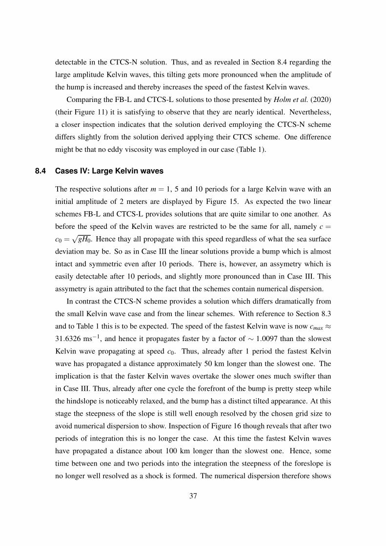
8.4 Cases IV: Large Kelvin waves

The respective solutions after m = 1, 5 and 10 periods for a large Kelvin wave with an

initial amplitude of 2 meters are displayed by Figure 15. As expected the two linear

schemes FB-L and CTCS-L provides solutions that are quite similar to one another. As

before the speed of the Kelvin waves are restricted to be the same for all, namely c =

c0 =√

gH0. Hence thay all propagate with this speed regardless of what the sea surface

deviation may be. So as in Case III the linear solutions provide a bump which is almost

intact and symmetric even after 10 periods. There is, however, an assymetry which is

easily detectable after 10 periods, and slightly more pronounced than in Case III. This

assymetry is again attributed to the fact that the schemes contain numerical dispersion.

In contrast the CTCS-N scheme provides a solution which differs dramatically from

the small Kelvin wave case and from the linear schemes. With reference to Section 8.3

and to Table 1 this is to be expected. The speed of the fastest Kelvin wave is now cmax ≈31.6326 ms−1, and hence it propagates faster by a factor of ∼ 1.0097 than the slowest

Kelvin wave propagating at speed c0. Thus, already after 1 period the fastest Kelvin

wave has propagated a distance approximately 50 km longer than the slowest one. The

implication is that the faster Kelvin waves overtake the slower ones much swifter than

in Case III. Thus, already after one cycle the forefront of the bump is pretty steep while

the hindslope is noticeably relaxed, and the bump has a distinct tilted appearance. At this

stage the steepness of the slope is still well enough resolved by the chosen grid size to

avoid numerical dispersion to show. Inspection of Figure 16 though reveals that after two

periods of integration this is no longer the case. At this time the fastest Kelvin waves

have propagated a distance about 100 km longer than the slowest one. Hence, some

time between one and two periods into the integration the steepness of the foreslope is

no longer well resolved as a shock is formed. The numerical dispersion therefore shows

37

1500 1750 2000 2250 2500 2750 3000 3250 3500x [km]

-0.5

0

0.5

1

1.5

2

2.5

Sea s

urf

ace d

evia

tio

n [

m]


FB-L

1500 1750 2000 2250 2500 2750 3000 3250 3500x [km]

0

1

2

Sea s

urf

ace d

evia

tio

n [

m]


CTCS-L

1500 1750 2000 2250 2500 2750 3000 3250 3500x [km]

0

1

2

Sea s

urf

ace d

evia

tio

n [

m]


CTCS-NCase IV: A = 25 m**2/s

a)

b)

c)

Figure 15: Case IV: As Figure 14, but for large Kelvin waves.

itself as a trailing wave lagging behind the shock, not unlike what happened in Case I.

Moreover, once the shock is formed it moves with a speed cmax > c0, and consequently

the shock appears to lead the initial bump as displayed by Figures 15 and 16. This is again

similar to the nonlinear Case I solution.

Furthermore, the nonlinear solution provided by the CTCS-N scheme disagree with

the solution provided by Holm et al. (2020) (their Figure 12). It is also more in line

with the solutions derived by using the KP and CDKLM schemes for the large Kelvin

wave case. In fact, filtering the CTCS-N solution as shown by Figure 17 the result is

38

1500 1750 2000 2250 2500 2750 3000 3250 3500x [km]

0

1

2

Sea s

urf

ace d

evia

tio

n [

m]

Initial condition1 period2 periods3 periods5 periods10 periods


Figure 16: Case IV: The nonlinear solution after various periods. Otherwise as Figure 15.

indeed very similar to their solutions derived using the KP and CDKLM schemes (their

Figure 12). Interestingly, the nonlinear CTCS solution of Holm et al. (2020) appears to

be mirroring the CTCS-N solution, that is, the Kelvin waves are moving westward rather

than eastward.

1500 1750 2000 2250 2500 2750 3000 3250 3500x [km]

0

1

2

Sea s

urf

ace d

evia

tio

n [

m]

10 periodsFiltered


Figure 17: Case IV: The filtered sea surface deviation on top of the unfiltered one. The filter is

an unweighted, moving average filter using 31 points. Otherwise as Figure 15.

It may be argued that increasing the resolution (decreasing the space increments)

would improve the CTCS-N solution. However, since the CTCS-N scheme is a con-

vergent scheme (Røed, 2019, Section 4.9, page 57) the numerical solution approaches the

true solution only in the limit when the space increments and time step go to zero. Thus,

39

decreasing the space increments only postpones the onset of the waves due to numerical

dispersion.

The numerical dispersion appearing as the shock forms (Figure 16) are indeed similar

to the numerical dispersion experienced in Case I (Figure 8). However, in Case I the

front was already established initially and the numerical dispersion in the form of trailing

waves appeared immediately. In Case IV the shock establishes itself only after some time

into the integration, and hence also the trailing waves caused by the numerical dispersion.

Another similarity with Case I is that the amplitude of the dispersive waves grows in time

and although the solution is stable even after 10 periods of integration it may eventually

go unstable in a numerical sense later on.

Figure 18: Case IV: The sea surface deviation after 10 periods of integration. A is the eddy

viscosity coefficient. The distance in the east-west direction is truncated.

There are some differences though. Recall that in Case I the solution is one-dimensional,

while in Case IV it is two-dimensional right from the start in that the amplitude of the ini-

tial bump decreases with increasing distance from the southern wall (Figure 7). As a

result the fastest Kelvin wave some distance away from the southern wall moves slower

than those closer to the southern wall. Thus, a longer and longer time will be needed in

order for the fastest wave to overtake the slowest one as one proceed away from the south-

ern wall. The dispersive waves therefore shows up first close to the southern wall and then

progressivly later as one moves away from the wall. The two-dimensional impression is

40

therefore of waves that appears to be arching backwards away from the southern wall as

depicted by Figure 18 after 10 periods of integration. At any specific time into the inte-

gration the amplitude of the waves are therefore decreasing away from the southern wall.

In addition Case IV includes the effect of rotation that enables the bump to be balanced

geostrophically.

Also present in the solution after 10 periods of integration is a striking wave like

pattern lagging far behind the shock (Figures 16 and 18). As revealed by Figure 19 the

depicted waves at the forefront appear to be reflected at the northern wall and to continue

toward the southern wall. On their way to be reflected at the southern wall they disturb

the tail of the solution which explains the trailing wave pattern.

(a) (b) (c)

(d) (e) (f)

Figure 19: Case IV: As Figure 18, but showing the initial condition (a), the solution after 1 period

(b), 2 periods (c), 3 periods (d), 5 periods (e), and 10 periods (f) of integration.

9 Summary and some final remarks

Considered are linear and nonlinear solutions to the shallow water equations for four

cases, namely Case I: Dam break on a wet domain without rotation, Case II: Rossby

41

adjustment, Case III: Small Kelvin waves, and Case IV: Large Kelvin waves. These cases

correspond to and are identical to four of the cases performed by Holm et al. (2020). Thus,

a comparison of their results and those presented here are facilitated.

The cases are all run in a two-dimensional basin with a flat bottom oriented so that

the x-axis runs from west to east and the y-axis from south to north (cf. Figures 2 and 3).

The southern and northern boundaries are closed, reflecting walls, while the eastern and

western boundaries are open. All cases are started from a specified initial state, which in

Cases I and II is unbalanced. In Cases III and IV the initial state is balanced (geostrophic

balance).

Two of the schemes studied here, namely the linear FB-L scheme and the nonlinear

CTCS-N scheme are identical to two of the schemes investigated by Holm et al. (2020),

specifically the schemes they denoted FBL and CTCS. In addition solutions derived us-

ing a linear version of the CTCS-N scheme, called the CTCS-L scheme, is provided for

comparison with the linear FB-L scheme. All the above mentioned schemes are finite dif-

ference schemes. However, Holm et al. (2020) also included two finite volume schemes,

namely the KP scheme and the CDKLM scheme credited to Kurganov and Petrova (2007)

and Chertok et al. (2018), respectively.

In all four cases the linear FB-L and CTCS-L solutions are for all practical purposes

identical to each other and to the linear (FBL) solution of Holm et al. (2020). In Cases II

and III this is also true concerning the nonlinear CTCS-N scheme and the similar nonlin-

ear CTCS scheme of Holm et al. (2020). However, in Cases I and IV they differ radically.

Both of these cases contain a shock. Since the finite difference schemes used here contain

numerical dispersion expected trailing waves appear in both of these cases in the solu-

tions provided by the CTCS-N scheme. However, these dispersive waves are not present

in the CTCS solutions of Holm et al. (2020) in Case I. Moreover, except for the expected

dispersive waves, the Case I solution provided by the CTCS-N scheme is more in line

with the solution derived using the KP and CDKLM schemes of Holm et al. (2020) (their

figure 6) and the analytic solution. Regarding Case IV, which treats the highly nonlinear

Kelvin wave case, the CTCS-N solution after one cycle is almost identical to the CDKLM

solution of Holm et al. (2020). At this stage in the integration the slope of the front, which

later forms a shock, is still well resolved and the numerical dispersion negligible. How-

ever, as the shock forms between cycle one and two the numerical dispersion becomes

evident in the form of trailing waves of growing amplitudes lagging behind the shock. On

the northern hemisphere the Kelvin waves moves with the boundary to its right, that is

42

1500 1750 2000 2250 2500 2750 3000 3250 3500x [km]

0

1

2

Sea s

urf

ace d

evia

tio

n [

m]



1500 1750 2000 2250 2500 2750 3000 3250 3500x [km]

0

1

2

Sea s

urf

ace d

evia

tio

n [

m]



1500 1750 2000 2250 2500 2750 3000 3250 3500x [km]

0

1

2

Sea s

urf

ave d

evia

tio

n [

m]



1500 1750 2000 2250 2500 2750 3000 3250 3500x [km]

0

1

2

Sea s

urf

ace d

evia

tio

n [

m]



1500 1750 2000 2250 2500 2750 3000 3250 3500x [km]

0

1

2

Sea s

urf

ace d

evia

tio

n [

m]



a)

b) c)

d) e)

Figure 20: Case IV: The sea surface deviation for various choices of the eddy viscosity coefficient

A (unit m2/s). a) A = 25, b) A = 0, c) A = 500, d) A = 1000, and e) A = 2500.

eastward in Case IV. This is the case regarding both the CTCS-N solution studied here

and the solutions derived using the finite volume schemes KP and CDKLM studied by

Holm et al. (2020). Also looking at the CTCS solution of Holm et al. (2020) the Kelvin

waves do appear to be moving eastward, but the tilting of the dome is opposite to that of

all the other nonlinear schemes. Interestingly the CTCS solution of Holm et al. (2020) do

contain the trailing dispersive waves in Case IV where the shock forms.

It may be argued that by increasing the eddy viscosity the dispersive waves my be

damped and thereby produce a result more akin to the filtered solution shown by Figure

17, and hence more in line with the KP and CDKLM solutions of Holm et al. (2020). An

attempt in this direction is displayed by Figure 20. As portrayed an increase in the eddy

viscosity does damp the amplitude of the trailing dispersive waves. However, at the same

time the speed of the front is slowed down and the amplitude of the dominant Kelvin

43

waves are decreased. Thus, increasing the eddy viscosity does not make the solution look

more like the results using finite volume schemes KP and CDKLM. Thus, these more

recent and modern finite volume schemes are superior to the finite difference schemes in

the sense that they avoid the numerical dispersion, and thereby improves the ability to

handle steep fronts and shocks numerically.

Nevertheless, the finite difference, nonlinear solution presented by Holm et al. (2020)

(their CTCS scheme) is dramatically different from the CTCS-N solutions for Case I and

IV presented in the present study, and also dramatically different from their solutions

using the finite volume schemes KP and CDKLM. Holm et al. (2020) ascribes this dif-

ference being due to numerical dispersion. This is contrary to the conclusion reached

and discussed in Section 8.4. There it was concluded that the scheme CTCS-N provided

solutions more similar to the KP and CDKLM solutions in both Case I and Case IV. It is

therefore concluded that the erratic behaviour of the CTCS scheme being due to numerical

dispersion is misguided. Rather something must be incorrect in their GPU implementa-

tion of the CTCS scheme. Nonetheless the main conclusion reached by Holm et al. (2020)

stands to be correct, namely that the KP and CDKLM are superior to the finite difference

schemes regarding resolving steep fronts and shocks.

44

Acknowledgements

This work has been funded by the Research Council of Norway under grant no. 250935/O70

(GPU Ocean).

References

References

Chapman, D. C. (1985), Numerical treatment of cross-shelf open boundaries in a

barotropic coastal ocean model, J. Phys. Oceanogr., 15, 1060–1075.

Chertok, A., M.Dudzinski, A. Kurganov, and M. Lukacova-Medvidova (2018), Well-

balanced schemes for the shallow water equations with Coriolis forces, Numerische

Mathematik, 138, 939–973, doi:10.1007/s00211-017-0928-0.

Davies, H. C. (1976), A lateral boundary formulation for multilevel prediction models,

Quart. J. Roy. Meteor. Soc., 102, 405–418, doi:10.1002/qj.49710243210.

Delestre, O., C. Lucas, P.-A. Ksinant, F. Darboux, and C. Laguerre (2013), Swashes:

a compilation of Shallow Water Analytic Solutions for Hydraulic and Environmen-

tal Studies, International Journal for Numerical Methods in Fluids, 72(3), 269–300,

ff10.1002/fld.3741ff. ffhal-00628246v6f.

Engedahl, H. (1995a), Use of the flow relaxation scheme in a three-dimensional baroclinic

ocean model with realistic topography, Tellus, 47A, 365–382.

Holm, H. H., A. R. Brodtkorb, G. Brostrøm, K. H. Christensen, and M. L. Sæ-

tra (2020), Evaluation of selected finite-difference and finite-volume approaches to

rotational shallow-water flow, Commun. Comput. Phys., 27(4), 1234–1274, doi:

https://doi.org/10.4208/cicp.OA-2019-0033.

Jamart, B. M., and J. Ozer (1986), Numerical boundary layers and spurious residual flows,

J. Geophys. Res., 91, 10,621–10,631.

Kurganov, A., and G. Petrova (2007), A second order well-balanced positivity preserving

central-upwind scheme for the Saint-Venant system, Comm. Math. Sci., 5, 133–160.

45

Martinsen, E. A., B. Gjevik, and L. P. Røed (1979), A numerical model for long barotropic

waves and storm surges along the western coast of Norway, J. Phys. Oceanogr., 9,

1126–1138.

Mesinger, F., and A. Arakawa (1976), Numerical methods used in atmospheric models,

GARP Publication Series No. 17, 64 p., World Meteorological Organization, Geneva,

Switzerland.

Palma, E. D., and R. P. Matano (2000), On the implementation of open boundary condi-

tions to a general circulation model: The 3-d case., J. Geophys. Res., 105, 8605–8627.

Phillips, N. A. (1959), An example of nonlinear computational instability, in The Atmo-

sphere and the Sea in motion, edited by B. Bolin, pp. 501–504, Rockefeller Institute

Press, New York.

Røed, L. P. (2019), Atmospheres and Ocean on Computers: Fundamental Numerical

Methods for Geophysical Fluid Dynamics, Springer Textbooks in Earth Sciences, Ge-

ography and Environment, 275 pp., Springer Nature Switzerland, doi:10.1007/978-3-

319-93864-6.

Røed, L. P., and C. K. Cooper (1987), A study of various open boundary conditions for

wind-forced barotropic numerical ocean models, in Three-dimensional models of ma-

rine and estuarine dynamics, Elsevier Oceanography Series, vol. 45, edited by J. C. J.

Nihoul and B. M. Jamart, pp. 305–3, Elsevier Science Publishers B.V.

Rossby, C. G. (1937), On the mutual adjustment of pressure and velocity distributions in

certain simple current systems, J. Mar. Res., 1, 15–28.

Rossby, C. G. (1938), On the mutual adjustment of pressure and velocity distributions in

certain simple current systems. Part II, J. Mar. Res., 1, 239–263.

Sielecki, A. (1968), An energy-conserving numerical scheme for the solution of the storm

surge equations, Mon. Weather Rev., 96, 150–156.

A The FORTRAN program

46

The FORTRAN program consists of the main program nonlinear_swe and eight sub-

routines init, savef, store, ctcs-n, euler-n, ctcs-l, euler-l and fbl. The subrou-

tines ctcs-n, ctcs-l and fbl contains the algorithms for the the three schemes CTCS-

N, CTCS-L and FB-L, as their names suggest. The two additional schemes are linear

and nonlinear versions of the Euler schemes nessecary to avoid the initial problem of the

CTCS-N and CTCS-L schemes (cf. Sections 5.2 and 5.3). All subroutines are called from

the main program nonlinear_swe.

A.1 The main program nonlinear_swe.f90

program nonlinear_swe

implicit none

!---------------------------------------------------------------

! Front matter

! Declarations:

! Assign logical unit numbers (lun) of files

integer, parameter :: olunh1 = 11 ! outfileh1




integer, parameter :: olunhe = 15 ! outfilehe

integer, parameter :: olunhp = 16 ! outfilehp

integer, parameter :: olunu1 = 21 ! outfileu1




integer, parameter :: olunue = 25 ! outfileue

integer, parameter :: olunup = 26 ! outfileup

integer, parameter :: olunv1 = 31 ! outfilev1




integer, parameter :: olunve = 35 ! outfileve

integer, parameter :: olunvp = 36 ! outfilevp

integer, parameter :: olunhov = 40 ! outfilehov

47

integer, parameter :: llun = 41 ! logfile

! Space and time dimensions

integer, parameter :: np = 4 ! # times variables saved

integer :: jmax ! # of cells along x-axis

integer :: kmax ! # of cells along y-axis

! Runtime parameters (independent of case)

integer, parameter :: Ng = 10 ! # space increments FRS

integer, parameter :: nfl = 5000 ! time steps in one cycle

integer, parameter :: nhov = 50 ! # time steps Hovmøller

real, parameter :: g = 9.81 ! Gravitational acceleration

real, parameter :: ff = 1.2E-04 ! Coriolis parameter

! Runtime constants (dependent on case)

integer :: n2 ! # of time steps to complete one cycles

integer :: n3 ! # of time steps to complete five cycles

integer :: n4 ! # of time steps to complete ten cycles

integer :: ntmax ! Maximum # of time steps

real :: A ! Eddy viscosity coefficient [m**2/s]

real :: f ! Coriolis parameter [1/s]

real :: dx ! Space increment along x-axis [m]

real :: dy ! Space increment along y-axis [m]

real :: x0 ! Center of maximum initial eta [m]

real :: y0 ! Location of maximum eta

real :: H0 ! Equilibrium depth (flat bottom) [m]

real :: c0 ! Phase speed of linear Kelvin wave [m/s]

real :: Lx ! Length of basin east-west direction

real :: Ly ! Length of basin north-south direction

real :: dt ! Time step [s]

real :: dt2 ! Twice the time step

real :: eta0 ! Initial maximum sea surface deviation [m]

real :: Lr ! Rossby’s deformation radius [m]

integer :: kp ! Cell # at which Up,Vp,hp, & etap are saved

! Auxiliary variables

integer :: nt ! # of time levels of scheme

real :: time ! Time in seconds

48

real :: htime ! Time in hours

real :: dtime ! Time in days

integer :: n,ntime ! Time step counters

integer :: iold,icur,inew,isave ! Time level counters

integer :: j,k ! Space increment (j,k)

integer :: jp1 ! Auxiliary counter

integer :: nsave ! # of time steps to save

! Auxiliary runtime constants used in subroutine update

real :: pru,prv ! Constants used in pressure terms

real :: ax,ay,a4x,a4y ! Constants used in nonlinear terms

real :: mixu,mixv ! Constants used in mixing terms

real :: R ! Constant due to Dufort-Frankel

real :: corU,fdt ! Help factors Coriolis term

! Auxiliary variables used in subroutine update:

real :: CU,CV ! Coriolis terms

real :: PU,PV ! Pressure terms

real :: AUx,AUy,AVx,AVy ! Advection terms

real :: MU,MV ! Eddy viscosity terms

real :: Uhjpk,Uhjk,UAjk,VAjk,hAjk ! Help variables

real :: UAjkm,VAjkm,hAjkm ! Help variables

real :: UAjmk,VAjmk,hAjmk,Vhjkp,Vhjk ! Help variables

! Auxiliary constants and arrays used in subroutine init:

real :: arg11,arg12 ! Help variables

real :: argx,argy ! Help variables

real :: arg4,LL,DD ! Help constants

! Dimension of allocateable arrays:

! Thickness points x-axis in meters [m]

real, allocatable, dimension (:) :: x

! Thickness points x-axis in kilometers [km]

real, allocatable, dimension (:) :: xkm

! Thickness points along y-axis [m]

real, allocatable, dimension (:) :: y

! Thickness points along y-axis [km]

real, allocatable, dimension (:) :: ykm

49

! Initial left-hand depth Case A [m]

real, allocatable, dimension (:) :: Hl

! Initial right-hand depth Case A [m]

real, allocatable, dimension (:) :: Hr

! Offshore transport [m**2/s]

real, allocatable, dimension (:,:,:) :: U

! As U, but at specified times [m**2/s]

real, allocatable, dimension (:,:,:) :: Ue

! As Ue, but at auxiliary points [m**2/s]

real, allocatable, dimension (:,:,:) :: Up

! Alongshore transport [m**2/s]

real, allocatable, dimension (:,:,:) :: V

! As V, but at specified times [m**2/s]

real, allocatable, dimension (:,:,:) :: Ve

! As Ve, but at auxiliary points [m**2/s]

real, allocatable, dimension (:,:,:) :: Vp

! Thickness of water column [m]

real, allocatable, dimension (:,:,:) :: h

! As h, but at specified times [m**2/s]

real, allocatable, dimension (:,:,:) :: he

! As he, but at auxiliary points [m]

real, allocatable, dimension (:,:,:) :: hp

! Sea surface deviation from equilibrium [m]

real, allocatable, dimension (:,:,:) :: eta

! As eta, but at the specified times [m]

real, allocatable, dimension (:,:,:) :: etae

! As etae, but at auxiliary points [m]

real, allocatable, dimension (:,:,:) :: etap

! Allocateable auxiliary arrays used in subroutine init:

real, allocatable, dimension(:) :: alf ! Relax para in x

real, allocatable, dimension(:) :: alfl ! Relax para left in x

real, allocatable, dimension(:) :: alfr ! Relax para right

real, allocatable, dimension(:) :: arg1 ! y dependence

real, allocatable, dimension(:) :: arg2 ! x dependence

50

real, allocatable, dimension(:) :: arg3 ! As arg1


real, allocatable, dimension(:) :: corV ! Factor Coriolis term

! Flags

integer :: icase ! 1,2,3,4 => Cases I,II,III,IV

integer :: ischeme ! 1,2,3 => Schemes FB-L, CTCS-L,CTCS-N

integer :: ishap ! 0,1 => no filter, Shapiro filter applied

integer :: iev ! 0,1 => No eddy viscosity (EV), EV applied

integer :: ibc ! 1,2 => Cyclic,FRS boundary condition

! Character strings:

character(LEN=80) :: outfileh1 ! 1st (initial) etae field

character(LEN=80) :: outfileu1 ! 1st (initial) Ue field

character(LEN=80) :: outfilev1 ! 1st (initial) Ve field

character(LEN=80) :: outfileh2 ! 2nd etae field

character(LEN=80) :: outfileu2 ! 2nd Ue field

character(LEN=80) :: outfilev2 ! 2nd Ve field

character(LEN=80) :: outfileh3 ! 3rd etae field

character(LEN=80) :: outfileu3 ! 3rd Ue field

character(LEN=80) :: outfilev3 ! 3rd Ve field

character(LEN=80) :: outfileh4 ! 4th etae field

character(LEN=80) :: outfileu4 ! 4th Ue field

character(LEN=80) :: outfilev4 ! 4th Ve field

character(LEN=80) :: outfilehe ! etae along x (k=2)

character(LEN=80) :: outfileue ! Ue along x (k=2)

character(LEN=80) :: outfileve ! Ve along x (k=2)

character(LEN=80) :: outfilehp ! etap along x (k=2)

character(LEN=80) :: outfileup ! Up along x (k=2)

character(LEN=80) :: outfilevp ! Vp along x (k=2)

character(LEN=80) :: outfilehov ! Hovmoller file

character(LEN=80) :: logfile ! Holds the logrun info

integer :: res ! Status file operations

51

! End declarations

!---------------------------------------------------------------

! Assign meaningful names to the outfiles and the logfile

outfileh1 = "Initial_eta-results.dat"

outfileu1 = "Initial_u-results.dat"

outfilev1 = "Initial_v-results.dat"

outfileh2 = "2nd_eta-results.dat"

outfileu2 = "2nd_u-results.dat"

outfilev2 = "2nd_v-results.dat"

outfileh3 = "3rd_eta-results.dat"

outfileu3 = "3rd_u-results.dat"

outfilev3 = "3rd_v-results.dat"

outfileh4 = "4th_eta-results.dat"

outfileu4 = "4th_u-results.dat"

outfilev4 = "4th_v-results.dat"

outfilehe = "etae-results.dat"

outfileue = "ue-results.dat"

outfileve = "ve-results.dat"

outfilehp = "etap-results.dat"

outfileup = "up-results.dat"

outfilevp = "vp-results.dat"

outfilehov = "Hovmoller-results.dat"

logfile = "log.dat"

!---------------------------------------------------------------

! Open files

! 1: Files related to eta

open(unit=olunh1,file=outfileh1,form="formatted",iostat=res)

if(res /= 0) then ! An error has occured

print*, "Error in opening outfileh1, status: ", res

stop ! Stop the program

endif




52


endif





endif





endif

open(unit=olunhe,file=outfilehe,form="formatted",iostat=res)


print*, "Error in opening outfilehe, status: ", res


endif

open(unit=olunhp,file=outfilehp,form="formatted",iostat=res)


print*, "Error in opening outfilehp, status: ", res


endif

! 2: Files related to U

open(unit=olunu1,file=outfileu1,form="formatted",iostat=res)


print*, "Error in opening outfileu1, status: ", res


endif





endif


53




endif





endif

open(unit=olunue,file=outfileue,form="formatted",iostat=res)


print*, "Error in opening outfileue, status: ", res


endif

open(unit=olunup,file=outfileup,form="formatted",iostat=res)


print*, "Error in opening outfileup, status: ", res


endif

! 3: Files related to V

open(unit=olunv1,file=outfilev1,form="formatted",iostat=res)


print*, "Error in opening outfilev1, status: ", res


endif





endif





54

endif





endif

open(unit=olunve,file=outfileve,form="formatted",iostat=res)


print*, "Error in opening outfileve, status: ", res


endif

open(unit=olunvp,file=outfilevp,form="formatted",iostat=res)


print*, "Error in opening outfilevp, status: ", res


endif

open(unit=olunhov,file=outfilehov,form="formatted",iostat=res)


print*, "Error in opening outfilehov, status: ", res


endif

! End open files

!---------------------------------------------------------------

! Set flags

write(6,*) ’Choose case to run (icase):’

write(6,*) ’1 => Case A: Breaking of a dam, no rotation’

write(6,*) ’2 => Case B: Adjustment under gravity, rotating’

write(6,*) ’3 => Case C: Small Kelvin waves’

write(6,*) ’4 => Case D: Large Kelvin waves’

read(5,*) icase

if( (icase > 4).or.(icase < 1) ) then

stop ’icase out of bounds. Start over.’

endif

if( (icase == 1).or.(icase == 2) ) then ! Case I and II

55

ibc = 2 ! FRS at east-west boundaries

else ! Case III and IV

ibc = 1 ! Cyclic east-west

endif

write(6,*) ’Choose scheme (ischeme):’

write(6,*) ’1 => FB-L, 2 => CTCS-L, 3 => CTCS-N)’

read(5,*) ischeme

if( (ischeme > 3).or.(ischeme < 1) ) then

stop ’ischeme out of bounds. Start over.’

endif

if(ischeme == 1) then ! FB-L

iev = 0 ! No eddy viscosity

else ! CTCS-L and CTCS-N

write(6,*) ’Choose whether to apply Eddy Viscosity (iev):’

write(6,*) ’0 => no EV, 1 => apply EV’

read(5,*) iev

if( (iev > 1).or.(iev < 0) ) then

stop ’iev out of bounds. Start over.’

endif

endif

write(6,*) ’Apply Shapiro filter (ishap)? 0 => No, 1 => Yes’

read(5,*) ishap

if( (ishap > 1).or.(ishap < 0) ) then

stop ’ishap out of bounds. Start over.’

endif

! End set flags

!---------------------------------------------------------------

! Specify # of time levels in scheme

if(ischeme == 1) then

nt = 2 ! FB-L has only two time levels

else

nt = 3 ! The 2 CTCS schemes have three time levels

endif

!---------------------------------------------------------------

56

! Specify # of cells (including ghost cells) in x and y

! directions and time levels for saving of variables

if(icase == 1) then ! Case I: Breaking of a dam (wet)

jmax = 501

kmax = 52

kp = 2

n2 = 200 ! Final = 2 s

n3 = 400 ! Final = 4 s

n4 = 600 ! Final = 6 s

ntmax= n4 + 1

elseif(icase == 2) then ! Case II: Adjustment under gravity

jmax = 801

kmax = 1002

kp = 501

n2 = 864 ! = 1 day

n3 = 1728 ! = 3 days

!n3 = 64800 ! = 75 days

!n4 = 129600 ! = 150 days

ntmax= n4 + 1

else ! Case III/IV: Small/Large Kelvin waves

jmax = 1001

kmax = 202

kp = 2

!n2 = nfl ! Testing

!n3 = 2*nfl ! Testing

!n4 = 3*nfl ! Testing

n2 = nfl ! Final = # to complete one cycles

n3 = 5*nfl ! Final = # to complete five cycles

n4 = 10*nfl ! Final = # to complete ten cycles

ntmax= n4 + 1

endif

!---------------------------------------------------------------

! Allocate space for variables

allocate (x(jmax), STAT=res)

57

if(res /= 0) then

print*, ’Error in allocating space for x, status: ’, res

stop

endif

allocate (xkm(jmax), STAT=res)

if(res /= 0) then

print*, ’Error in allocating space for xkm, status: ’, res

stop

endif

allocate (y(kmax), STAT=res)

if(res /= 0) then

print*, ’Error in allocating space for y, status: ’, res

stop

endif

allocate (ykm(kmax), STAT=res)

if(res /= 0) then

print*, ’Error in allocating space for ykm, status: ’, res

stop

endif

allocate (Hl(kmax), STAT=res)

if(res /= 0) then


stop

endif

allocate (Hr(kmax), STAT=res)

if(res /= 0) then


stop

endif

allocate (U(jmax,kmax,nt), STAT=res)

if(res /= 0) then

print*, ’Error in allocating space for U, status: ’, res

stop

endif

58

allocate (Ue(jmax,kmax,np), STAT=res)

if(res /= 0) then

print*, ’Error in allocating space for Ue, status: ’, res

stop

endif

allocate (Up(jmax,kmax,np), STAT=res)

if(res /= 0) then

print*, ’Error in allocating space for Up, status: ’, res

stop

endif

allocate (V(jmax,kmax,nt), STAT=res)

if(res /= 0) then

print*, ’Error in allocating space for V, status: ’, res

stop

endif

allocate (Ve(jmax,kmax,np), STAT=res)

if(res /= 0) then

print*, ’Error in allocating space for Ve, status: ’, res

stop

endif

allocate (Vp(jmax,kmax,np), STAT=res)

if(res /= 0) then

print*, ’Error in allocating space for Vp, status: ’, res

stop

endif

allocate (h(jmax,kmax,nt), STAT=res)

if(res /= 0) then

print*, ’Error in allocating space for h, status: ’, res

stop

endif

allocate (he(jmax,kmax,np), STAT=res)

if(res /= 0) then

print*, ’Error in allocating space for he, status: ’, res

stop

59

endif

allocate (hp(jmax,kmax,np), STAT=res)

if(res /= 0) then

print*, ’Error in allocating space for hp, status: ’, res

stop

endif

allocate (eta(jmax,kmax,nt), STAT=res)

if(res /= 0) then

print*, ’Error in allocating space for eta, status: ’, res

stop

endif

allocate (etae(jmax,kmax,np), STAT=res)

if(res /= 0) then

print*, ’Error in allocating space for etae, status: ’, res

stop

endif

allocate (etap(jmax,kmax,np), STAT=res)

if(res /= 0) then

print*, ’Error in allocating space for etap, status: ’, res

stop

endif

allocate (corV(kmax), STAT=res)

if(res /= 0) then

print*, ’Error in allocating space for corV, status: ’, res

stop

endif

allocate (alf(jmax), STAT=res)

if(res /= 0) then

print*, ’Error in allocating space for alf, status: ’, res

stop

endif

allocate (alfl(jmax), STAT=res)

if(res /= 0) then

print*, ’Error in allocating space for alfl, status: ’, res

60

stop

endif

allocate (alfr(jmax), STAT=res)

if(res /= 0) then

print*, ’Error in allocating space for alfr, status: ’, res

stop

endif

! End allocating variables

!---------------------------------------------------------------

! Specify runtime parameters and constants

if(icase == 1) then ! Case I

f = 0.*ff ! [1/s]

dx = 0.02 ! [m]

dy = 0.02 ! [m]

Lx = (jmax-1)*dx ! [m]

Ly = (kmax-2)*dy ! [m]

x0 = Lx/2. ! [m]

y0 = Ly/2. ! [m]

H0 = 0.003 ! [m]

A = 0.1 ! [m**2/s]

c0 = sqrt(g*H0) ! [m/s]

dt = 0.01 ! [s]

eta0 = 0.002 ! [m]

Lr = 0.0 ! [m]

elseif(icase == 2) then ! Case II

f = ff ! [1/s]

dx = 5.0E+4 ! [m] = 50 km

dy = 5.0E+4 ! [m] = 50 km



x0 = Lx/2. ! [m]

y0 = Ly/2. ! [m]

H0 = 1.0E+3 ! [m] = 1 km

A = 25. ! [m**2/s]

61

c0 = sqrt(g*H0) ! [m/s]

dt = 100. ! [s]

Lr = c0/f ! [m]

eta0 = 0.2 ! [m]

Hl = H0 ! [m]

Hr = H0 ! [m]

elseif(icase == 3) then ! Case III

f = ff ! [1/s]

dx = 5.0E+3 ! [m]

dy = 1.0E+4 ! [m]



x0 = Lx/2. ! [m]

y0 = -0.5*dy ! [m]

H0 = 1.0E+2 ! [m]

A = 25. ! [m**2/s]

c0 = sqrt(g*H0) ! [m/s]

dt = Lx/(nfl*c0) ! [s]

Lr = c0/f ! [m]

eta0 = 0.05 ! [m]

Hl = H0 ! [m]

Hr = H0 ! [m]

else ! Case IV

f = ff ! [1/s]

dx = 5.0E+3 ! [m]

dy = 1.0E+4 ! [m]

!dx = 2.5E+3 ! [m], Half mesh size

!dy = 0.5E+4 ! [m], Half mesh size



x0 = Lx/2. ! [m]

y0 = -0.5*dy ! [m]

H0 = 1.0E+2 ! [m]

A = 25. ! [m**2/s]

62

c0 = sqrt(g*H0) ! [m/s]

dt = Lx/(nfl*c0) ! [s]

Lr = c0/f ! [m]

eta0 = 2.0 ! [m]

Hl = H0 ! [m]

Hr = H0 ! [m]

endif

arg4 = 0.5*eta0

dt2 = 2.*dt ! [s]

! End specifying runtime parameters and constants

!---------------------------------------------------------------

! Open, write to, and close logfile

open(unit=llun,file=logfile,form="formatted",iostat=res)


print*, "Error in opening logfile, status: ", res


endif

write(unit=llun,FMT=’(1X,A37,1X,4I6,1X,A7)’,iostat=res) &

’Flags : icase, ischeme, iev, ishap : ’, &

icase,ischeme,iev,ishap,’-’


print*, "Error in writing Flags to logfile, status: ", res


endif

write(unit=llun,FMT=’(1X,A37,1X,I20,1X,A7)’,iostat=res) &

’# of time steps to complete 1 cycle: ’, Nfl,’-’


print*, "Error in writing nfl to logfile, status: ", res


endif

write(unit=llun,FMT=’(1X,A37,1X,F20.6,1X,A7)’,iostat=res) &

’Length Lx of basin : ’, Lx,’m’


print*, "Error in writing Lx to logfile, status: ", res

63


endif


’Gravitational acceleration : ’, g,’m^2/s^2’


print*, "Error in writing g to logfile, status: ", res


endif


’Coriolis parameter f : ’, f,’m^2/s’


print*, "Error in writing f to logfile, status: ", res


endif


’Equilibrium depth H0 : ’, H0,’m’


print*, "Error in writing H0 to logfile, status: ", res


endif

write(unit=llun,FMT=’(1X,A37,1X,2F20.6,1X,A7)’,iostat=res) &

’Space increments dx, dy : ’,dx, dy, ’m’


print*, "Error in writing dx to logfile, status: ", res


endif


’Time step dt : ’, dt,’s’


print*, "Error in writing dt to logfile, status: ", res


endif


’Deformation radius : ’, Lr,’m’

64


print*, "Error in writing Lr to logfile, status: ", res


endif


’Wave speed c0 : ’, c0,’m/s’


print*, "Error in writing c0 to logfile, status: ", res


endif

! Close the logfile

close(unit=llun)

! End opening, writing to, and closing the logfile

!---------------------------------------------------------------

! Location of the auxiliary points along the x and y axes.

! Origo is the auxiliary point in grid cell (1,1).

do j=1,jmax

x(j) = (j-1)*dx

if(icase == 1) then

xkm(j) = x(j) ! Case I dimension is only 10 [m]

else

xkm(j) = x(j)/1000.

endif

end do

do k=1,kmax

y(k) = (k-1)*dy

ykm(k) = y(k)/1000.

end do

!---------------------------------------------------------------

! Relaxation parameter(s) needed for FRS boundary condition

do j=1,jmax

arg11 = (j-1)/3.

arg12 = (jmax-j)/3.

x(j) = (j-1)*dx

65

if(j <= Ng) then

alf(j) = 1. - tanh(arg11)

elseif(j >= jmax-Ng) then

alf(j) = 1. - tanh(arg12)

else

alf(j) = 0.

endif

end do

! End front matter

!---------------------------------------------------------------

! Initialization

! Time step, time and time level counters

ntime = 0

time = 0.

htime = 0.

dtime = 0.

iold = 1

icur = 2


inew = 2 ! FB-L has 2 time levels

else

inew = 3

endif

! Variables and equilibrium depth

call init(U,V,h,eta,Up,Vp,hp,etap,Ue,Ve,etae,x,y,Hl,Hr, &

jmax,kmax,nt,np,icase,arg4,H0,x0,y0, &

dx,dy,Lr,c0,f,eta0)

! Save initial variables

nsave = 1

call savef(U,V,eta,xkm,Up,Vp,hp,etap,Ue,Ve,etae, &

jmax,kmax,inew,nt,np,nsave,ishap,ibc,H0,res)

! End initialization

66

!---------------------------------------------------------------

do ntime=1,ntmax ! Start the time loop

print *, ’Working on time step no.: ’, ntime

! New time in seconds, hours and days

time = time+dt

htime = time/3600.

dtime = htime/24.

! Update variables U,V,h,eta including the boundaries

if(ischeme == 1) then ! FB-L (linear)

call fbl(U,V,h,eta,x,y,alf,Hl,Hr,jmax,kmax,iold,inew, &

nt,ntime,ibc,dx,dy,dt,f,g,H0,x0,y0)

elseif(ischeme == 2) then ! CTCS-L (linear)

! Euler step to avoid initial problem of CTCS

if(ntime == 1) then

call euler_l(U,V,h,eta,x,y,alf,Hl,Hr,jmax,kmax, &

iold,icur,nt,ntime,iev,ibc,dx,dy,dt, &

f,g,A,eta0,H0,x0,y0)

else

call ctcs_l(U,V,h,eta,x,y,alf,Hl,Hr,jmax,kmax, &

iold,icur,inew,nt,ntime,iev,ibc, &

dx,dy,dt,dt2,f,g,A,eta0,H0,x0,y0)

endif

else ! CTCS-N (non-linear)

! Euler step to avoid initial problem of CTCS

if(ntime == 1) then

call euler_n(U,V,h,eta,x,y,alf,Hl,Hr,jmax,kmax, &

iold,icur,nt,ntime,ibc,iev,dx,dy,dt, &


else

call ctcs_n(U,V,h,eta,x,y,alf,Hl,Hr,jmax,kmax, &

iold,icur,inew,nt,ntime,ibc,iev, &

dx,dy,dt,dt2,f,g,A,eta0,H0,x0,y0)

endif

endif

67

! Should we write to the Hovmoller file?

if(mod(ntime,nhov) == 0) then

write (unit =olunhov,fmt =’(1001F12.4)’, iostat =res) &

(eta(j,2,inew),j=1,jmax)


print*, ’Error saving Hovmoller-results.dat:’

print*, ’status: ’, res


endif

endif

! Should we save the results?

if( ntime == n2 ) then

nsave = 2

go to 13

elseif( ntime == n3 ) then

nsave = 3

go to 13

elseif( ntime == n4 ) then

nsave = 4

go to 13

else

go to 23

endif

13 call savef(U,V,eta,xkm,Up,Vp,hp,etap,Ue,Ve,etae, &

jmax,kmax,inew,nt,np,nsave,ishap,ibc,H0,res) &

! Swap indices

23 if(ischeme == 1) then ! FB-L scheme

isave = inew

inew = iold

iold = isave

else

if(ntime == 1) then ! Euler scheme

continue

else ! CTCS-L & CTCS-N scheme

68

isave = inew

inew = iold

iold = icur

icur = isave

endif

endif

end do

! End of time loop

!---------------------------------------------------------------

! Write results to files

write(6,*) ’Writing results to files’

call store(Ue,Ve,etae,Up,Vp,hp,etap,xkm,jmax,kmax,np,kp, &

icase,olunh1,olunu1,olunv1,olunh2,olunu2,olunv2, &

olunh3,olunu3,olunv3,olunh4,olunu4,olunv4, &

olunhe,olunue,olunve,olunhp,olunup,olunvp,res)

! End writing to files

!---------------------------------------------------------------

! End program in an orderly fashion

! Close output and log files

close(unit=olunh1)

close(unit=olunh2)

close(unit=olunh3)

close(unit=olunh4)

close(unit=olunhe)

close(unit=olunhp)

close(unit=olunu1)

close(unit=olunu2)

close(unit=olunu3)

close(unit=olunu4)

close(unit=olunue)

close(unit=olunup)

close(unit=olunv1)

close(unit=olunv2)

close(unit=olunv3)

69

close(unit=olunv4)

close(unit=olunve)

close(unit=olunvp)

close(unit=olunhov)

2 format(3I4,1X,4F10.4)

if( icase == 1 ) then

write(6,*) ’Case I solved successfully’

elseif( icase == 2) then

write(6,*) ’Case II solved successfully’


write(6,*) ’Case III solved successfully’


write(6,*) ’Case IV solved successfully’

endif


write(6,*) ’The Forward-Backward scheme (FB-L) was used’

elseif( ischeme == 2 ) then

if(iev == 0) then

write(6,*) ’The CTCS-L scheme was employed. No EV added’

elseif( iev == 1 ) then

write(6,*) ’The CTCS-L scheme was employed. EV added’

endif

else

if(iev == 0) then

write(6,*) ’The CTCS-N scheme was employed. No EV added’

elseif( iev == 1 ) then

write(6,*) ’The CTCS-N scheme was employed. EV added’

endif

endif

if( ishap == 1 ) then

write(6,*) ’The Shapiro filter applied to results.’

else

write(6,*) ’No Shapiro filter applied.’

endif

70

end program nonlinear_swe ! End of main program

!---------------------------------------------------------------

71

A.2 Subroutine init.f90

!///////////////////////////////////////////////////////////////

!// //

!// Subroutine init //

!// //

!// Called by main program //

!// //

!// Purpose: //

!// //

!// To initialize volume transports (U,V), water column //

!// thickness (h), and sea surface deviation (eta). //

!// //

!///////////////////////////////////////////////////////////////

subroutine init(U,V,h,eta,Up,Vp,hp,etap, &

Ue,Ve,etae,x,y,Hl,Hr, &

jmax,kmax,nt,np,icase,arg4, &

H0,x0,y0,dx,dy,Lr,c0,f,eta0)

implicit none

integer, intent(IN) :: jmax,kmax,nt,np,icase

integer :: j,k,n,jp1,res

real, intent(IN) :: H0,x0,y0,dx,dy,Lr,c0,f,eta0,arg4

real, dimension(jmax,kmax,nt) :: U,V,h,eta

real, dimension(jmax,kmax,np) :: Up,Vp,hp,etap

real, dimension(jmax,kmax,np) :: Ue,Ve,etae

real, dimension(jmax) :: x

real, dimension(kmax) :: y,Hl,Hr

real :: argx,argy,LL,DD

real, allocatable, dimension(:) :: arg1 ! Initial y dependence

real, allocatable, dimension(:) :: arg2 ! Initial x dependence



!---------------------------------------------------------------

72

! Allocate allocatable variables

allocate (arg1(kmax), STAT=res)

if(res /= 0) then

print *, ’Error in allocating space for arg1, status:’, res

stop

endif

allocate (arg2(jmax), STAT=res)

if(res /= 0) then


stop

endif


if(res /= 0) then


stop

endif


if(res /= 0) then


stop

endif

! End allocating variables

!---------------------------------------------------------------

! Give a default value (a funny one though) to all variables in

! all grid cells

! Variables U, V, h and eta at all time levels

do n = 1,nt

do k=1,kmax

do j=1,jmax

U(j,k,n) = 999.

V(j,k,n) = 999.

h(j,k,n) = 999.

eta(j,k,n) = 999.

end do

73

end do

end do

! Variables Up, Vp. hp, etap, Ue, Ve, etae to be saved and

! written to file np times

do n = 1,np

do k=1,kmax

do j=1,jmax

Up(j,k,n) = 999.

Vp(j,k,n) = 999.

hp(j,k,n) = 999.

etap(j,k,n) = 999.

Ue(j,k,n) = 999.

Ve(j,k,n) = 999.

etae(j,k,n) = 999.

end do

end do

end do

! End giving all variables a default value

!---------------------------------------------------------------

! Assign initial values to variables for each case

do n=1,nt

if( icase == 1 ) then ! Case A: Abrupt step

! h and eta

do k=1,kmax-1

do j=1,jmax

if(x(j) < x0) then

eta(j,k,n) = eta0

elseif(x(j) == x0) then

eta(j,k,n) = 0.

else

eta(j,k,n) = - eta0

endif

h(j,k,n) = eta(j,k,n) + H0

74

end do

Hl(k) = h(1,k,n)

Hr(k) = h(jmax,k,n)

end do

! U and V

do k=1,kmax

do j=1,jmax

U(j,k,n) = 0.

V(j,k,n) = 0.

end do

end do

elseif( icase == 2 ) then ! Case B

! Compute some helpful constants

LL = 15.*dx

DD = 50.*dx

! eta and h

do k=1,kmax

argy = y(k) - 0.5*dy - y0

do j=1,jmax

argx = x(j) - 0.5*dx - x0

eta(j,k,n) = arg4*( 1. + &

tanh((DD - sqrt( argx*argx + argy*argy) )/LL))


U(j,k,n) = 0.

V(j,k,n) = 0.

end do

Hl(k) = h(1,k,n)

Hr(k) = h(jmax,k,n)

end do

else ! Cases C and D

! Compute some helpful arrays

do k=1,kmax

argy = y(k) - 0.5*dy - y0

arg1(k) = - (1./Lr)*sqrt( argy**2. )

75

arg3(k) = 0.5*c0*sign( 1.,argy )

arg5(k) = arg4*exp( arg1(k) )

end do

do j=1,jmax

argx = x(j) - 0.5*dx - x0

arg2(j) = tanh( (3./Lr)*( Lr - sqrt( argx*argx ) ) )

end do

! eta and h

do k=2,kmax-1

do j=2,jmax

eta(j,k,n) = arg5(k)*( 1. + arg2(j) )


end do

! Cyclic boundary condition

eta(1,k,n) = eta(jmax,k,n)

h(1,k,n) = h(jmax,k,n)

end do

! U

do k=2,kmax-1

do j=2,jmax

if(j == jmax) then ! Cyclic boundary condition

jp1 = 2

else

jp1 = j+1

endif

U(j,k,n) = arg3(k)*( eta(jp1,k,n) + eta(j,k,n) )

end do

! Cyclic boundary condition

U(1,k,n) = U(jmax,k,n)

end do

! Closed boundary condition U

do j=1,jmax

U(j,1,n) = - U(j,2,n)

U(j,kmax,n) = - U(j,kmax-1,n)

76

end do

! V including boundaries

do k=1,kmax-1

do j=1,jmax

V(j,k,n) = 0.

end do

end do

endif

end do

! End assigning real values to variables for all cases

!---------------------------------------------------------------

return

end subroutine init

77

A.3 Subroutine savef.f90

!///////////////////////////////////////////////////////////////

!// //

!// Subroutine savef //

!// //

!// Called by main program: nonlinear_swe //

!// //

!// Purpose: //

!// //

!// To save the variables for later storing at their //

!// respective grid points (etae, Ue and Ve) //

!// //

!///////////////////////////////////////////////////////////////

subroutine savef(U,V,eta,xkm,Up,Vp,hp,etap,Ue,Ve,etae, &

jmax,kmax,inew,nt,np,nsave,ishap,ibc,H0,res)

implicit none

integer, intent(in) :: jmax,kmax

integer, intent(in) :: inew,nt,np,nsave,ishap

integer :: j,k,res,jp1,ibc

real, dimension (jmax,kmax,nt) :: U,V,h,eta

real, dimension(jmax) :: xkm

real, dimension(jmax,kmax,np) :: Up,Vp,hp,etap,Ue,Ve,etae

real :: H0

!---------------------------------------------------------------

! Save variables

if(ishap == 0) then ! Raw model results

do k=2,kmax-1

do j=1,jmax

etae(j,k,nsave) = eta(j,k,inew)

78

end do

end do

do k=1,kmax-1

do j=1,jmax

Ve(j,k,nsave) = V(j,k,inew)

end do

end do

do k=2,kmax-1

do j=1,jmax

Ue(j,k,nsave) = U(j,k,inew)

end do

end do

else ! ishap = 1 => Apply Shapiro filter

if(ibc == 1) then ! Cyclic boundary condition

do k=3,kmax-2

do j=2,jmax

if(j == jmax) then

jp1 = 2

else

jp1=j+1

endif

etae(j,k,nsave) = 0.25*( eta(jp1,k,inew) + &

eta(j-1,k,inew) + &

eta(j,k+1,inew) + &

eta(j,k-1,inew) )

Ue(j,k,nsave) = 0.25*( U(jp1,k,inew) + &

U(j-1,k,inew) + &

U(j,k+1,inew) + &

U(j,k-1,inew) )

Ve(j,k,nsave) = 0.25*( V(jp1,k,inew) + &

V(j-1,k,inew) + &

V(j,k+1,inew) + &

V(j,k-1,inew) )

end do

79

etae(1,k,nsave) = etae(jmax,k,nsave) ! j=1

Ue(1,k,nsave) = Ue(jmax,k,nsave)

Ve(1,k,nsave) = Ve(jmax,k,nsave)

end do

do j=2,jmax ! k=2, k=kmax-1

if(j == jmax) then

jp1 = 2

else

jp1=j+1

endif

etae(j,2,nsave) = eta(j,2,inew) + &

0.25*( eta(jp1,2,inew) - &

2.*eta(j,2,inew) + &

eta(j-1,2,inew) )

Ue(j,2,nsave) = U(j,2,inew) + &

0.25*( U(jp1,2,inew) - &

2.*U(j,2,inew) + &

U(j-1,2,inew) )

Ve(j,2,nsave) = V(j,k,inew) + &

0.25*( V(jp1,k,inew) - &

2.*V(j,k,inew) + &

V(j-1,k,inew) )

Ve(j,1,nsave) = 0.

etae(j,kmax-1,nsave) = eta(j,kmax-1,inew) + &

0.25*( eta(jp1,kmax-1,inew) - &

2.*eta(j,kmax-1,inew) + &

eta(j-1,kmax-1,inew) )

Ue(j,kmax-1,nsave) = U(j,kmax-1,inew) + &

0.25*( U(jp1,kmax-1,inew) - &

2.*U(j,kmax-1,inew) + &

U(j-1,kmax-1,inew) )

Ve(j,kmax-1,nsave) = 0.

end do

! j=1, k=2

80

etae(1,2,nsave) = etae(jmax,2,nsave)

Ue(1,2,nsave) = Ue(jmax,2,nsave)

Ve(1,2,nsave) = Ve(jmax,2,nsave)

! j=1, k=kmax-

etae(1,kmax-1,nsave) = etae(jmax,kmax-1,nsave) 1

Ue(1,kmax-1,nsave) = Ue(jmax,kmax-1,nsave)

Ve(1,kmax-1,nsave) = 0.

else ! Flow Relaxation Scheme

do k=3,kmax-2

do j=2,jmax-1

jp1=j+1

etae(j,k,nsave) = 0.25*( eta(jp1,k,inew) + &

eta(j-1,k,inew) + &

eta(j,k+1,inew) + &

eta(j,k-1,inew) )

Ue(j,k,nsave) = 0.25*( U(jp1,k,inew) + &

U(j-1,k,inew) + &

U(j,k+1,inew) + &

U(j,k-1,inew) )

Ve(j,k,nsave) = 0.25*( V(jp1,k,inew) + &

V(j-1,k,inew) + &

V(j,k+1,inew) + &

V(j,k-1,inew) )

end do

etae(1,k,nsave) = eta(1,k,inew) ! j=1

Ue(1,k,nsave) = U(1,k,inew)

Ve(1,k,nsave) = V(1,k,inew)

etae(jmax,k,nsave) = eta(jmax,k,inew) ! j=jmax

Ue(jmax,k,nsave) = U(jmax,k,inew)

Ve(jmax,k,nsave) = V(jmax,k,inew)

end do

do j=2,jmax-1 ! k=1,2 and k=kmax-1

jp1=j+1

etae(j,2,nsave) = eta(j,2,inew) + &

81

0.25*( eta(jp1,2,inew) - &

2.*eta(j,2,inew) + &

eta(j-1,2,inew) )

Ue(j,2,nsave) = U(j,2,inew) + &

0.25*( U(jp1,2,inew) - &

2.*U(j,2,inew) + &

U(j-1,2,inew) )

Ve(j,2,nsave) = V(j,k,inew) + &

0.25*( V(jp1,k,inew) - &

2.*V(j,k,inew) + &

V(j-1,k,inew) )

Ve(j,1,nsave) = 0.

etae(j,kmax-1,nsave) = eta(j,kmax-1,inew) + &

0.25*( eta(jp1,kmax-1,inew) - &

2.*eta(j,kmax-1,inew) + &

eta(j-1,kmax-1,inew) )

Ue(j,kmax-1,nsave) = U(j,kmax-1,inew) + &

0.25*( U(jp1,kmax-1,inew) - &

2.*U(j,kmax-1,inew) + &

U(j-1,kmax-1,inew) )

Ve(j,kmax-1,nsave) = 0.

end do

etae(1,2,nsave) = eta(1,2,inew) ! j=1, k=2

Ue(1,2,nsave) = U(1,2,inew)

Ve(1,2,nsave) = V(1,2,inew)

etae(1,kmax-1,nsave) = eta(1,kmax-1,inew)

Ue(1,kmax-1,nsave) = U(1,kmax-1,inew)

Ve(1,kmax-1,nsave) = 0.

etae(jmax,2,nsave) = eta(jmax,2,inew) ! j=jmax, k=2

Ue(jmax,2,nsave) = U(jmax,2,inew)

Ve(jmax,2,nsave) = V(jmax,2,inew)

etae(jmax,kmax-1,nsave) = eta(jmax,kmax-1,inew)

Ue(jmax,kmax-1,nsave) = U(jmax,kmax-1,inew)

Ve(jmax,kmax-1,nsave) = 0.

82

endif

endif

! End saving variables

!---------------------------------------------------------------

return

end subroutine savef

83

A.4 Subroutine store.f90

!///////////////////////////////////////////////////////////////

!// //

!// Subroutine store //

!// //


!// //

!// Purpose: //

!// //

!// To store the results to be plotted //

!// //

!///////////////////////////////////////////////////////////////

subroutine store(Ue,Ve,etae,Up,Vp,hp,etap,xkm,jmax,kmax,np, &

kp,icase,olunh1,olunu1,olunv1, &

olunh2,olunu2,olunv2,olunh3,olunu3,olunv3, &

olunh4,olunu4,olunv4,olunhe,olunue,olunve, &

olunhp,olunup,olunvp,res)

implicit none

integer, intent(in) :: jmax,kmax,np,kp,icase

integer, intent(in) :: olunhp,olunup,olunvp

integer, intent(in) :: olunhe,olunue,olunve

integer, intent(in) :: olunh1,olunu1,olunv1




integer :: j,k,n,res

real, dimension(jmax) :: xkm

real, dimension(jmax,kmax) :: U,V,h,eta

real, dimension(jmax,kmax,np) :: Ue,Ve,etae,Up,Vp,hp,etap

!---------------------------------------------------------------

! Write to files

if(icase == 1) then ! Case I: Breaking of a dam. No rotation

84

do k=2,kmax-1

! eta: etae fields

write (unit =olunh1, fmt =’(501F12.7)’, iostat =res) &

(etae(j,k,1),j=1,jmax)


print *, &

’Error saving to initial_eta-results, status:’, res

stop ! stop the program

endif




print *, &

’Error saving to 2nd_eta-results, status:’, res


endif




print *, &

’Error saving to 3rd_eta-results, status:’, res


endif




print *, &

’Error saving to 4th_eta-results, status:’, res


endif

! U: Ue fields

write (unit =olunu1, fmt =’(501F12.7)’, iostat =res) &

(Ue(j,k,1),j=1,jmax)


85

print *, &

’Error saving to initial_U-results, status:’, res


endif




print *, &

’Error saving to 2nd_U-results, status:’, res


endif




print *, &

’Error saving to 3rd_U-results, status:’, res


endif




print *, &

’Error saving to 4th_U-results, status:’, res


endif

! V: Ve field

write (unit =olunv1, fmt =’(501F12.7)’, iostat =res) &

(Ve(j,k,1),j=1,jmax)


print *, &

’Error saving to initial_V-results, status:’, res


endif


86



print *, &

’Error saving to 2nd_V-results, status:’, res


endif




print *, &

’Error saving to 3rd_V-results, status:’, res


endif




print *, &

’Error saving to 4th_V-results, status:’, res


endif

end do

elseif (icase == 2) then ! Case II: Adjustment under gravity

do k=2,kmax-1

! eta: etae fields




print *, &



endif




87

print *, &



endif




print *, &



endif




print *, &



endif

! U: Ue fields




print *, &



endif




print *, &



endif


88



print *, &



endif




print *, &



endif

! V: Ve field




print *, &



endif




print *, &



endif




print *, &



89

endif




print *, &



endif

end do

else ! Case III/IV: Small/large Kelvin waves

do k=2,kmax-1

! eta: etae fields




print *, &



endif




print *, &



endif




print *, &



endif


90



print *, &



endif

! U: Ue fields




print *, &



endif




print *, &



endif




print *, &



endif




print *, &



91

endif

! V: Ve field




print *, &



endif




print *, &



endif




print *, &



endif




print *, &



endif

end do

endif

!

! eta: Raw data along southern boundary (k=kp) at grid

92

! points (etae) and at auxiliary points (etap)

do j=1,jmax

write (unit =olunhe, fmt =’(5F12.7)’, iostat =res) xkm(j) &

,etae(j,kp,1), etae(j,kp,2), etae(j,kp,3), etae(j,kp,4)


print *, &

’Error saving to file etae-results, status:’, res


endif

write (unit =olunhe, fmt =’(5F12.7)’, iostat =res) xkm(j) &

,etap(j,kp,1), etap(j,kp,2), etap(j,kp,3), etap(j,kp,4)


print *, &

’Error saving to file etap-results, status:’, res


endif

end do

! U: Raw data along southern boundary (k=kp) at grid

! points (Ue) and at auxiliary points (Up)

do j=1,jmax

write (unit =olunue, fmt =’(5F12.7)’, iostat =res) xkm(j) &

,Ue(j,kp,1), Ue(j,kp,2), Ue(j,kp,3), Ue(j,kp,4)


print *, &

’Error saving to file Ue-results, status:’, res


endif

write (unit =olunup, fmt =’(5F12.7)’, iostat =res) xkm(j) &

,Up(j,kp,1), Up(j,kp,2), Up(j,kp,3), Up(j,kp,4)


print *, &

’Error saving to file Up-results, status:’, res


endif

93

end do

! V: Raw data along southern boundary (k=kp) at grid

!points (Ve) and at auxiliary points (Vp)

do j = 1,jmax

write (unit =olunve, fmt =’(5F12.7)’, iostat =res) xkm(j) &

,Ve(j,kp,1), Ve(j,kp,2), Ve(j,kp,3), Ve(j,kp,4)


print *, &

’Error saving to file Ve-results, status:’, res


endif

write (unit =olunvp, fmt =’(5F12.7)’, iostat =res) xkm(j) &

,Vp(j,kp,1), Vp(j,kp,2), Vp(j,kp,3), Vp(j,kp,4)


print *, &

’Error saving to file Vp-results, status:’, res


endif

end do

return

end subroutine store

94

A.5 Subroutine ctcs-n.f90

!///////////////////////////////////////////////////////////////

!// //

!// Subroutine ctcs_n //

!// //


!// //

!// Purpose: //

!// //

!// To update thickness and volume transports using the //

!// nonlinear CTCS scheme. //

!// First step (ntime=1) uses subroutine Euler //

!// //

!///////////////////////////////////////////////////////////////

subroutine ctcs_n(U,V,h,eta,x,y,alf,Hl,Hr,jmax,kmax,iold,icur, &

inew,nt,ntime,ibc,iev,dx,dy,dt,dt2, &


implicit none

!---------------------------------------------------------------

! Front matter

! Declarations

integer, intent(in) :: jmax,kmax,iold,icur,inew

integer, intent(in) :: nt,ntime,ibc,iev

real, intent(in) :: dx,dy,dt,dt2,f,g,A,eta0,H0

real, intent(in) :: x0,y0

integer :: j,k,n,jp1


real, dimension(kmax) :: corV,Hl,Hr,y

real, dimension(jmax) :: alf,x

real :: CU,CV,PU,PV,MU,MV

real :: ax,ay,pru,prv,a4x,a4y

real :: mixu,mixv,R,corU

95

real :: AUx,AUy,AVx,AVy

real :: Uhjpk,Uhjk,UAjk,UAjkm

real :: VAjk,VAjkm,hAjk,hAjkm

real :: UAjmk,VAjmk,Vhjk,Vhjkm,hAjmk

!---------------------------------------------------------------

! Compute constants needed

ax = dt2/dx

ay = dt2/dy

pru = 0.5*g*ax

prv = 0.5*g*ay

mixu = iev*dt2*A/(dx*dx)

mixv = iev*dt2*A/(dy*dy)

R = 1./( 1. + mixu + mixv )

a4x = 0.25*ax

a4y = 0.25*ay

corU = 0.5*f*dt

do k=1,kmax

corV(k) = 0.5*f*dt

end do

corV(2) = f*dt

corV(kmax-1) = f*dt

corV(kmax) = f*dt

! End front matter

!---------------------------------------------------------------

! Update variables

! Recall the cyclic boundary condition east-west.

! So when j=jmax all references to j+1 must be replaced by 2

!-------------------------------------------------------------

! 1: h and eta

do k=2,kmax-1

do j=2,jmax

! Update h

h(j,k,inew) = h(j,k,iold) - &

96

ax*( U(j,k,icur) - U(j-1,k,icur) ) - &

ay*( V(j,k,icur) - V(j,k-1,icur) )

! Update eta

eta(j,k,inew) = h(j,k,inew) - H0

end do


h(1,k,inew) = h(jmax,k,inew)

eta(1,k,inew) = eta(jmax,k,inew)

else

do j=1,jmax ! FRS boundary condition

if(x(j) <= x0) then

h(j,k,inew) = ( 1. - alf(j) )*h(j,k,inew) + &

alf(j)*Hl(k)

else


alf(j)*Hr(k)

endif


end do

endif

end do

!-------------------------------------------------------------

! 2: U

do k=2,kmax-1


do j=2,jmax

! Recall cyclic boundary condition east-west => all

! references to j+1 must be replaced by 2 when

! j = jmax

if(j == jmax) then

jp1 = 2

else

jp1 = j+1

endif

97

! Coriolis term U

CU = corV(k)*( V(j,k-1,icur) + V(j,k,icur) + &

V(jp1,k,icur) + V(jp1,k-1,icur) )

! Pressure term U

PU = - pru*( h(jp1,k,icur) + h(j,k,icur) )* &

( eta(jp1,k,icur) - eta(j,k,icur) )

! Advective, nonlinear flux terms U

Uhjpk = U(jp1,k ,icur) + U(j ,k ,icur)

Uhjk = U(j ,k ,icur) + U(j-1,k ,icur)

UAjk = U(j ,k+1,icur) + U(j ,k ,icur)

UAjkm = U(j ,k ,icur) + U(j ,k-1,icur)

VAjk = V(jp1,k ,icur) + V(j ,k ,icur)

VAjkm = V(jp1,k-1,icur) + V(j ,k-1,icur)

if(k == 2) then

hAjkm = 2.*( h(j,k,icur) + h(jp1,k,icur) )

else

hAjkm = h(j,k-1,icur) + h(j,k,icur) + &

h(jp1,k,icur) + h(jp1,k-1,icur)

endif

if(k == kmax-1) then

hAjk = 2.*( h(j,k,icur) + h(jp1,k,icur) )

else

hAjk = h(j,k,icur) + h(j,k+1,icur) + &

h(jp1,k+1,icur) + h(jp1,k,icur)

endif

AUx = - a4x*( ( (Uhjpk*Uhjpk)/h(jp1,k,icur) ) - &

( ( Uhjk*Uhjk )/h(j,k,icur) ) )

AUy = - ay*( ( (UAjk*VAjk )/hAjk ) - &

( ( UAjkm*VAjkm )/hAjkm ) )

! Mixing terms (Dufort-Frankel) U

MU = mixu*( U(jp1,k,icur) - U(j,k,iold) + &

U(j-1,k,icur) ) &

+ mixv*( U(j,k+1,icur) - U(j,k,iold) + &

U(j,k-1,icur) )

98

! Update U

U(j,k,inew) = ( U(j,k,iold) + CU + PU + &

AUx + AUy + MU )*R

end do

else ! FRS boundary condition

do j=1,jmax

U(j,k,inew) = (1. - alf(j))*U(j,k,inew) + alf(j)*0.

end do

endif

end do

! Closed boundary condition U

do j=1,jmax

U(j,1,inew) = - U(j,2,inew)

U(j,kmax,inew) = - U(j,kmax-1,inew)

end do

!-------------------------------------------------------------

! 3: V

corU = 0.5*f*dt

do k=2,kmax-2


do j=2,jmax



! j = jmax

if(j == jmax) then

jp1 = 2

else

jp1 = j+1

endif

! Coriolis term V

CV = - corU*( U(j-1,k,icur) + U(j-1,k+1,icur) + &

U(j,k+1,icur) + U(j,k,icur) )

! Pressure term V

PV = - prv*( h(j,k+1,icur) + h(j,k,icur) )* &

99

( eta(j,k+1,icur) - eta(j,k,icur) )

! The advective, non-linear flux terms V

UAjk = U(j ,k+1,icur) + U(j ,k ,icur)

UAjmk = U(j-1,k+1,icur) + U(j-1,k ,icur)

VAjk = V(jp1,k ,icur) + V(j ,k ,icur)

VAjmk = V(j ,k ,icur) + V(j-1,k ,icur)

Vhjk = V(j ,k+1,icur) + V(j ,k ,icur)

Vhjkm = V(j ,k ,icur) + V(j ,k-1,icur)

hAjk = h(j,k ,icur) + h(j,k+1,icur) + &

h(jp1,k+1,icur) + h(jp1,k,icur)

hAjmk = h(j-1,k,icur) + h(j-1,k+1,icur) + &

h(j,k+1,icur) + h(j,k,icur)

AVx = - ax*( UAjk*VAjk/hAjk - UAjmk*VAjmk/hAjmk )

AVy = - a4y*( Vhjk*Vhjk/h(j,k+1,icur) - &

Vhjkm*Vhjkm/h(j,k,icur) )

! Mixing terms (Dufort-Frankel) V

MV = mixu*( V(jp1,k,icur) - V(j,k,iold) + &

V(j-1,k,icur) ) &

+ mixv*( V(j,k+1,icur) - V(j,k,iold) + &

V(j,k-1,icur) )

! Update V

V(j,k,inew) = ( V(j,k,iold) + CV + PV + &

AVx + AVy + MV )*R

end do

else


V(j,k,inew) = (1. - alf(j))*V(j,k,inew) + alf(j)*0.

end do

endif

end do

! Closed boundary condition V

do j=1,jmax

V(j,1,inew) = 0.

V(j,kmax-1,inew) = 0.

100

end do

! End updating variables

!---------------------------------------------------------------

return

end subroutine ctcs_n

101

A.6 Subroutine euler-n.f90

!///////////////////////////////////////////////////////////////

!// //

!// Subroutine euler_n //

!// //


!// //

!// Purpose: //

!// //

!// To update thickness and volume transports for the first //

!// time step to avoid initial problem in CTCS-N //

!// //

!///////////////////////////////////////////////////////////////

subroutine euler_n(U,V,h,eta,x,y,alf,Hl,Hr,jmax,kmax, &

dx,dy,dt,iold,icur,nt,ntime,ibc,iev, &


implicit none

!---------------------------------------------------------------

! Front matter

! Declarations

integer, intent(in) :: jmax,kmax,iold,icur,nt,ntime

integer, intent(in) :: ibc,iev

real, intent(in) :: dx,dy,dt,f,g,A,eta0,H0,x0,y0





real :: AUx,AUy,AVx,AVy,MU,MV


real :: CU,CV,PU,PV

real :: dt2,ax,ay,pru,prv,a4x,a4y

real :: Uhjpk,Uhjk,UAjk,VAjk,hAjk

102

real :: UAjkm,VAjkm,hAjkmUAjmk,VAjmk

real :: hAjmk,Vhjkp,Vhjk

! Compute constants needed

ax = dt/dx

ay = dt/dy

pru = 0.5*g*ax

prv = 0.5*g*ay

a4x = 0.25*ax

a4y = 0.25*ay

mixu = iev*dt*A/(dx*dx)

mixv = iev*dt*A/(dy*dy)

! End front matter

!---------------------------------------------------------------

! Update variables

! 1: h and eta

do k=2,kmax-1

do j=2,jmax

! Update h

h(j,k,icur) = h(j,k,iold) - &

ax*( U(j,k,iold) - U(j-1,k,iold) ) - &

ay*( V(j,k,iold) - V(j,k-1,iold) )

! Update eta

eta(j,k,icur) = h(j,k,icur) - H0

end do


h(1,k,icur) = h(jmax,k,icur)

eta(1,k,icur) = eta(jmax,k,icur)

else


if(x(j) <= x0) then

h(j,k,icur) = ( 1. - alf(j) )*h(j,k,icur) + &

alf(j)*Hl(k)

103

else


alf(j)*Hr(k)

endif


end do

endif

end do

! 2: U

do k=1,kmax

corV(k) = 0.25*f*dt

end do

corV(2) = 0.5*f*dt

corV(kmax-1) = 0.5*f*dt

corV(kmax) = 0.5*f*dt

do k=2,kmax-1


do j=2,jmax



! j = jmax

if(j == jmax) then ! Cyclic bc

jp1 = 2

else

jp1 = j+1

endif

! Coriolis term

CU = corV(k)*( V(j,k-1,iold) + V(j,k,iold) + &

V(jp1,k,iold) + V(jp1,k-1,iold) )

! Pressure term

PU = - pru*( h(jp1,k,iold) + h(j,k,iold) )* &

( eta(jp1,k,iold) - eta(j,k,iold) )

! Advective, non-linear flux terms

104

Uhjpk = U(jp1,k,iold) + U(j,k,iold)

VAjk = V(jp1,k,iold) + V(j,k,iold)

Uhjk = U(j,k,iold) + U(j-1,k,iold)

UAjk = U(j,k+1,iold) + U(j,k,iold)

UAjkm = U(j,k,iold) + U(j,k-1,iold)

VAjkm = U(jp1,k-1,iold) + U(j,k-1,iold)

if(k == 2) then

hAjkm = 2.*( h(j,k,iold) + h(j+1,k,iold) )

else

hAjkm = h(j,k-1,iold) + h(j,k,iold) + &

h(jp1,k,iold) + h(jp1,k-1,iold)

endif

if(k == kmax-1) then

hAjk = 2.*( h(j,k,iold) + h(jp1,k,iold) )

else

hAjk = h(j,k,iold) + h(j,k+1,iold) + &

h(jp1,k+1,iold) + h(jp1,k,iold)

endif

AUx = - a4x*( ( (Uhjpk*Uhjpk)/h(jp1,k,iold) ) - &

( ( Uhjk*Uhjk )/h(j,k,iold) ) )

AUy = - ay*( ( (UAjk*VAjk )/hAjk ) - &

( ( UAjkm*VAjkm )/hAjkm ) )

! Mixing terms (ordinary second order)

MU = mixu*( U(jp1,k,iold) - 2.*U(j,k,iold) + &

U(j-1,k,iold) ) + &

mixv*( U(j,k+1,iold) - 2.*U(j,k,iold) + &

U(j,k-1,iold) )

! Update U

U(j,k,icur) = U(j,k,iold) + CU + PU + AUx + AUy + MU

end do

else

do j=1,jmax ! FRS boundary conditions

U(j,k,icur) = ( 1. - alf(j) )*U(j,k,icur) + alf(j)*0.

end do

105

endif

end do

! Impose closed boundary conditions

do j=1,jmax

U(j,1,icur) = - U(j,2,icur)

U(j,kmax,icur) = - U(j,kmax-1,icur)

end do

! 3: V

corU = 0.25*f*dt

do k=2,kmax-1


do j=2,jmax



! j = jmax

if(j == jmax) then ! Cyclic bc

jp1 = 2

else

jp1 = j+1

endif

! Coriolis term

CV = - corU*( U(j-1,k,iold) + U(j-1,k+1,iold) + &

U(j,k+1,iold) + U(j,k,iold) )

! Pressure

PV = - prv*( h(j,k+1,iold) + h(j,k,iold) )* &

( eta(j,k+1,iold) - eta(j,k,iold) )

! The advective, non-linear flux terms

UAjk = U(j,k+1,iold) + U(j,k,iold)

VAjk = V(jp1,k,iold) + V(j,k,iold)

hAjk = h(j,k,iold) + h(j,k+1,iold) + &

h(jp1,k+1,iold) + h(jp1,k,iold)

UAjmk = U(j-1,k+1,iold) + U(j-1,k,iold)

VAjmk = V(j,k,iold) + V(j-1,k,iold)

106

hAjmk = h(j-1,k,iold) + h(j-1,k+1,iold) + &

h(j,k+1,iold) + h(j,k,iold)

Vhjkp = V(j,k+1,iold) + V(j,k,iold)

Vhjk = V(j,k,iold) + V(j,k-1,iold)

AVx = - ax*( ( UAjk*VAjk )/hAjk - &

( UAjmk*VAjmk )/hAjmk )

AVy = - a4y*( ( Vhjkp*Vhjkp )/h(j,k+1,iold) - &

( Vhjk*Vhjk )/h(j,k,iold) )

! Mixing terms

MV = mixu*( V(jp1,k,iold) - 2.*V(j,k,iold) + &

V(j-1,k,iold) ) + &

mixv*( V(j,k+1,iold) - 2.*V(j,k,iold) + &

V(j,k-1,iold) )

! Update V

V(j,k,icur) = V(j,k,iold) + CV + PV + AVx + AVy + MV

end do

else ! FRS boundary conditions

do j=1,jmax

V(j,k,icur) = ( 1. - alf(j) )*V(j,k,icur) + alf(j)*0.

end do

endif

end do

! Closed boundary conditions

do j=1,jmax

V(j,1,icur) = 0.

V(j,kmax-1,icur) = 0.

end do


!---------------------------------------------------------------

return

end subroutine euler_n

107

108

A.7 Subroutine ctcs-l.f90

!///////////////////////////////////////////////////////////////

!// //

!// Subroutine ctcs_l //

!// //


!// //

!// Purpose: //

!// //

!// Updates thickness and transports using the linear CTCS //

!// scheme. First time step uses the subroutine Euler_linear. //

!// //

!///////////////////////////////////////////////////////////////

subroutine ctcs_l(U,V,h,eta,x,y,alf,Hl,Hr,jmax,kmax,iold,icur, &

inew,nt,ntime,iev,ibc,dx,dy,dt,dt2, &


implicit none

!---------------------------------------------------------------

! Front matter

! Declarations

integer, intent(in) :: jmax,kmax,iold,icur,inew

integer, intent(in) :: nt,ntime,iev,ibc

real, intent(in) :: dx,dy,dt,dt2,f,g,A,eta0

real, intent(in) :: H0,x0,y0





real :: CU,CV,PU,PV,MU,MV

real :: ax,ay,pru,prv,a4x,a4y


109

! Compute needed constants

ax = dt2/dx

ay = dt2/dy

pru = g*H0*ax

prv = g*H0*ay

mixu = iev*dt2*A/(dx*dx)

mixv = iev*dt2*A/(dy*dy)

R = 1./( 1. + mixu + mixv )

!

! End front matter

!---------------------------------------------------------------

! Update variables

! 1; h and eta

do k=2,kmax-1

do j=2,jmax

! Update h


ax*( U(j,k,icur) - U(j-1,k,icur) ) - &

ay*( V(j,k,icur) - V(j,k-1,icur) )

! Update eta


end do




else


if(x(j) <= x0) then


alf(j)*Hl(k)

else


alf(j)*Hr(k)

endif

110


end do

endif

end do

! 2: U

do k=1,kmax

corV(k) = 0.5*f*dt

end do

corV(2) = f*dt

corV(kmax-1) = f*dt

corV(kmax) = f*dt

do k=2,kmax-1


do j=2,jmax



! j = jmax

if(j == jmax) then

jp1 = 2

else

jp1 = j+1

endif

! Coriolis term U

CU = corV(k)*( V(j,k-1,icur) + V(j,k,icur) + &

V(jp1,k,icur) + V(jp1,k-1,icur) )

! Pressure term U

PU = - pru*( eta(jp1,k,icur) - eta(j,k,icur) )

! Mixing terms U (Dufort-Frankel)

MU = mixu*( U(jp1,k,icur) - U(j,k,iold) + &

U(j-1,k,icur) ) &

+ mixv*( U(j,k+1,icur) - U(j,k,iold) + &

U(j,k-1,icur) )

! Update U

111

U(j,k,inew) = ( U(j,k,iold) + CU + PU + MU )*R

end do

U(1,k,inew) = U(jmax,k,inew)

else


U(j,k,inew) = ( 1. - alf(j) )*U(j,k,inew) + alf(j)*0.

end do

endif

end do

! Closed boundary conditions U

do j=1,jmax



end do

! 3: V

corU = 0.5*f*dt

do k=2,kmax-1


do j=2,jmax



! j = jmax

if(j == jmax) then

jp1 = 2

else

jp1 = j+1

endif

! Coriolis term V

CV = - corU*( U(j-1,k,icur) + U(j-1,k+1,icur) + &

U(j,k+1,icur) + U(j,k,icur) )

! Pressure term V

PV = - prv*( eta(j,k+1,icur) - eta(j,k,icur) )

! Mixing terms V (Dufort-Frankel)

112

MV = mixu*( V(jp1,k,icur) - V(j,k,iold) + &

V(j-1,k,icur) ) + &

mixv*( V(j,k+1,icur) - V(j,k,iold) + &

V(j,k-1,icur) )

! Update V

V(j,k,inew) = ( V(j,k,iold) + CV + PV + MV )*R

end do

V(1,k,inew) = V(jmax,k,inew)

else


V(j,k,inew) = ( 1. - alf(j) )*V(j,k,inew) + alf(j)*0.

end do

endif

end do

! Closed boundary condition V

do j=1,jmax

V(j,1,inew) = 0.


end do


!---------------------------------------------------------------

return

end subroutine ctcs_l

113

A.8 Subroutine euler-l.f90

!///////////////////////////////////////////////////////////////

!// //

!// Subroutine euler_l //

!// //


!// //

!// Purpose: //

!// //

!// To update variables using the linear version of the Euler //

!// scheme. //

!// //

!///////////////////////////////////////////////////////////////

subroutine euler_l(U,V,h,eta,x,y,alf,Hl,Hr,jmax,kmax, &

iold,icur,nt,ntime,iev,ibc,dx,dy,dt, &


implicit none

!---------------------------------------------------------------

! Front matter

! Declarations

integer, intent(in) :: jmax,kmax,iold,icur

integer, intent(in) :: nt,ntime,iev,ibc

real, intent(in) :: dx,dy,dt,f,g,A,eta0,H0,x0,y0





real :: CU,CV,PU,PV,MU,MV,fdt

real :: dt2,ax,ay,pru,prv,a4x

real :: a4y,mixu,mixv,R,corU

! Compute factor in front of the Coriolis terms

114

fdt = f*dt


ax = dt/dx

ay = dt/dy

pru = g*H0*ax

prv = g*H0*ay

mixu = iev*dt*A/(dx*dx)

mixv = iev*dt*A/(dy*dy)

! End front matter

!---------------------------------------------------------------

! Update variables

! 1: h and eta

do k=2,kmax-1

do j=2,jmax

! Update h

h(j,k,icur) = h(j,k,iold) - &



! Update eta


end do


h(1,k,icur) = h(jmax,k,icur)

eta(1,k,icur) = eta(jmax,k,icur)

else


if(x(j) <= x0) then


alf(j)*Hl(k)

else


alf(j)*Hr(k)

115

endif


end do

endif

end do

! 2: U

do k=1,kmax

corV(k) = 0.25*fdt

end do

corV(2) = 0.5*fdt

corV(kmax-1) = 0.5*fdt

corV(kmax) = 0.5*fdt

do k=2,kmax-1


do j=2,jmax



! j = jmax

if(j == jmax) then

jp1 = 2

else

jp1 = j+1

endif

! Coriolis term U



! Pressure term U

PU = - pru*( eta(jp1,k,iold) - eta(j,k,iold) )


MU = mixu*( U(jp1,k,iold) - 2.*U(j,k,iold) + &

U(j-1,k,iold) ) + &

mixv*( U(j,k+1,iold) - 2.*U(j,k,iold) + &

116

U(j,k-1,iold) )

! Update U

U(j,k,icur) = U(j,k,iold) + CU + PU + MU

end do

U(1,k,icur) = U(jmax,k,icur)

else


U(j,k,icur) = ( 1. - alf(j) )*U(j,k,icur) + alf(j)*0.

end do

endif

end do

! Impose closed boundary conditions on U

do j=1,jmax

U(j,1,icur) = - U(j,2,icur)

U(j,kmax,icur) = - U(j,kmax-1,icur)

end do

! 3: V

corU = 0.25*fdt

do k=2,kmax-1


do j=2,jmax



! j = jmax

if(j == jmax) then

jp1 = 2

else

jp1 = j+1

endif

! Coriolis term V

CV = - corU*( U(j-1,k,iold) + U(j-1,k+1,iold) + &

U(j,k+1,iold) + U(j,k,iold) )

! Pressure term V

117

PV = - prv*( eta(j,k+1,iold) - eta(j,k,iold) )


MV = mixu*( V(jp1,k,iold) - 2.*V(j,k,iold) + &

V(j-1,k,iold) ) + &

mixv*( V(j,k+1,iold) - 2.*V(j,k,iold) + &

V(j,k-1,iold) )

! Update V

V(j,k,icur) = V(j,k,iold) + CV + PV + MV

end do

V(1,k,icur) = V(jmax,k,icur)


do j=1,jmax

V(j,k,icur) = ( 1. - alf(j) )*V(j,k,icur) + alf(j)*0.

end do

endif

end do

! Impose closed boundary conditions on V

do j=1,jmax

V(j,1,icur) = 0.

V(j,kmax-1,icur) = 0.

end do


!---------------------------------------------------------------

return

end subroutine euler_l

118

A.9 Subroutine fbl.f90

!///////////////////////////////////////////////////////////////

!// //

!// Subroutine fbl //

!// //


!// //

!// Purpose: //

!// //

!// Updates thickness and transports using the Sielecki //

!// (Forward-Backward) scheme. //

!// //

!///////////////////////////////////////////////////////////////

subroutine fbl(U,V,h,eta,x,y,alf,Hl,Hr,jmax,kmax,iold,inew, &

nt,ntime,ibc,dx,dy,dt,f,g,H0,x0,y0)

implicit none

!---------------------------------------------------------------

! Front matter

! Declarations

integer, intent(in) :: jmax,kmax,iold,inew

integer, intent(in) :: nt,ntime,ibc

real, intent(in) :: dx,dy,dt,f,g,H0,x0,y0





real :: CU,CV,PU,PV,fdt

real :: dt2,ax,ay,pru,prv,a4x,a4y


real :: arg11,arg12

119


fdt = f*dt


ax = dt/dx

ay = dt/dy

pru = g*H0*ax

prv = g*H0*ay

! End front matter

!---------------------------------------------------------------

! Update variables


corU = 0.25*fdt

do k=1,kmax

corV(k) = 0.25*fdt

end do

corV(2) = 0.5*fdt

corV(kmax-1) = 0.5*fdt

corV(kmax) = 0.5*fdt

! 1: h and eta

do k=2,kmax-1

do j=2,jmax

! Update h




! Update eta


end do




120

else


if(x(j) <= x0) then


alf(j)*Hl(k)

else


alf(j)*Hr(k)

endif


end do

endif

end do

! 2: U

do k=2,kmax-1


do j=2,jmax



! j = jmax

if(j == jmax) then

jp1 = 2

else

jp1 = j+1

endif

! Coriolis term U



! Pressure term

PU = - pru*( eta(jp1,k,inew) - eta(j,k,inew) )

! Update U

U(j,k,inew) = U(j,k,iold) + CU + PU

end do


121

do j=1,jmax

U(j,k,inew) = ( 1. - alf(j) )*U(j,k,inew) + alf(j)*0.

end do

endif

end do

! Impose closed boundary conditions on U

do j=1,jmax



end do

! 3: V

do k=2,kmax-1


do j=2,jmax



! j = jmax

if(j == jmax) then

jp1 = 2

else

jp1 = j+1

endif

! Coriolis term V

CV = - corU*( U(j-1,k,inew) + U(j-1,k+1,inew) + &

U(j,k+1,inew) + U(j,k,inew) )

! Pressure

PV = - prv*( eta(j,k+1,inew) - eta(j,k,inew) )

! Update V

V(j,k,inew) = V(j,k,iold) + CV + PV

end do

V(1,k,inew) = V(jmax,k,inew)


do j=1,jmax

122

V(j,k,inew) = ( 1. - alf(j) )*V(j,k,inew) + alf(j)*0.

end do

endif

end do

! Impose closed boundary conditions on V

do j=1,jmax

V(j,1,inew) = 0.


end do


!---------------------------------------------------------------

return

end subroutine fbl

123

Date post:	25-Jan-2022
Category:	Documents
Upload:	others
View:	2 times
Download:	0 times

Evaluation of Selected Finite Difference Solutions to the ...

Documents