Evaluation of selected restoration technologies in degraded areas of the Mokala National Park, South Africa JJ Pelser 22841199 Dissertation submitted in fulfilment of the requirements for the degree Magister Scientiae in Environmental Sciences at the Potchefstroom Campus of the North-West University Supervisor: Prof K Kellner Co-supervisor: Mr ME Daemane May 2017
Transcript
Evaluation of selected restoration technologies in degraded areas of the Mokala National Park, South
Africa
JJ Pelser
22841199
Dissertation submitted in fulfilment of the requirements for the degree Magister Scientiae in Environmental Sciences at
the Potchefstroom Campus of the North-West University
Supervisor: Prof K Kellner Co-supervisor: Mr ME Daemane May 2017
i
Abstract
Degradation is a global problem and does not only affect the livelihood of people but
also the existence of fauna and flora. In Mokala National Park (MNP) extensive areas
of high potential grazing land have been degraded and are in urgent need of
restoration. The study was conducted in the Doornlaagte and Lilydale areas where
degradation is severe and restoration needed. Degradation of soils in these eroded
areas is the consequence of a loss of plant cover and density, mostly due to the
overgrazing of sensitive areas before the MNP was established and because the area
was used as a cattle farm. To prevent further degradation of the eroded areas, active
restoration technologies were implemented. Active restoration is the implementation
of techniques that involve the application of structures to improve the moisture and
nutrients in the soil, re-seeding, brush packing (placement of woody twigs on degraded
patches) and other methodologies to actively halt erosion and improve the ecosystem.
If these techniques are successfully implemented it will hopefully contribute to species
richness, diversity and soil vegetation cover.
The active restoration technologies that were implemented at Doornlaagte and
Lilydale include the brush packing technology, where branches of trees are packed on
top of the degraded soil; ponding, where hollows are made in a half-moon shape in
the soil to catch water and nutrients; and ponding & brush where the brush and
ponding restoration technologies are combined. Some areas were left open where no
restoration was applied. These served as control. The technologies were applied in
April 2014 and were monitored the day they were implemented, with the second
monitoring in October 2015 before the rainy season and the third monitoring at the
end of February 2016.
To achieve the mission of South African National Parks (SANParks) to develop,
manage and promote a system of National Parks that represents biodiversity and
heritage assets by applying best practice, environmental justice, benefit-sharing and
sustainable use, persons from the Biodiversity and Social Projects (BSP’s) programme
that work in MNP were used for the implementation of the restoration technologies
and for monitoring. The BSP programme is supported by the Department of
Environmental Affairs (DEA).
ii
Data were obtained from vegetation sampling at each technology and soil was
collected to determine the soil seed bank and to analyse soil parameters. The
Landscape Functional Analysis (LFA) monitoring technique was carried out to
evaluate any change in the functionality at the study sites.
Results show that although there were no significant differences, the density and
richness of the vegetation did increase especially in the ponding & brush restoration
technology at the Doornlaagte study site, whereas the ponding technology was the
best technology at the Lilydale study site. The soil seed bank analysis shows that the
most seed accumulated where the ponding & brush technology were applied in both
the Doornlaagte and Lilydale study sites. The LFA methodology showed that there
was an increase in the landscape functionality of both restoration study sites. The
change was mostly observed after the first year of restoration, as the area experienced
a severe drought which caused less changes to be observed in the second year of the
study.
Restoration is a long-term process and it is therefore recommended that this study be
Figure 6.9: The total patch area (m2) in the restoration site of Lilydale and how it
changed from 2014 to 2016. ......................................................................... 106
Figure 6.10: The Landscape Organization Index (LOI) of the Lilydale restoration site
from 2014 to 2016. ....................................................................................... 107
Figure 7.1: Areas around the ponding structure indicating where soil should and
should not be collected. 1 = where most vegetation establish in the pond. 2 =
where water flows past the restoration technologies. 3 = area where soil can be
collected to rebuild pond wall. Blue arrows indicate waterflow........................111
xv
List of tables
Table 1.1: Definitions of reclamation and re-vegetation 8
Table 3.1: Summary of the 11 SSA indicators and what their purposes are in the LFA............................................................................................................................50
xvi
List of abbreviations
BP Bare Patch
BSP Biodiversity and Social Project
CEC Cation exchangeable capacity
CA Correspondence analysis
Ca Calcium
[cmol (+)/kg)] Centimoles of positive charge per kilogram of soil
cm Centimetre
DCA Detrended correspondence analysis
DEA Department of Environmental Affairs
EC Electrical conductivity
EPWP Expanded Public Works Programme
FP Forb Patch
GP Grass Patch
GPS Global Positioning System
Ha Hectares
H2O Water
K Potassium
KCl Potassium Chloride
km Kilometre
LO Landscape Organisation
LOI Landscape Organisation Index
LFA Landscape Function Analysis
LP Litter Patch
m Metre
m2 Square metre
mg/kg Milligram per kilogram
Mg Magnesium
mm Millimetre
MNP Mokala National Park
mS/m MilliSiemens per metre
Na Sodium
NKu 3 Northern Upper Karoo
xvii
P & B Ponding & brush
P Phosphorus
PP Ponding Patch
SP Shrub Patch
pers. comm. Personal communication
SANParks South African National Parks
SD Standard Deviation
SSA Soil Surface Assessment
SSB Soil seed bank
SVk 4 Kimberley Thornveld
SVk 5 Vaalbos Rocky Shrubland
TTRP Trigger-Transfer-Reserve-Pulse
viz. Videlicet
1
Chapter 1 Introduction and Literature Review
1.1 General introduction
Arid and semi-arid regions make up more than 30% of the Earth’s surface (Okin, et
al., 2006; Bai et al., 2008). Large parts of these areas are not suitable for crop
production due to low and unpredictable rainfall patterns, especially in the summer
months. These arid and semi-arid areas are therefore used for livestock and/or game
production (Van den Berg & Kellner, 2010).
Two-thirds of the African continent’s drylands are exposed to degradation (ECOSOC,
2007) and according to Bojö (1995) many parts in Sub-Saharan Africa, need to be
restored to meet the demands of ecosystem services for improved human well-being
(MEA, 2005). Land degradation, particularly in drylands, has become of global
concern and affects many people (Adger et al., 2000). Arid and semi-arid areas
include up to 86% of the agricultural land in Southern Africa (Van den Berg & Kellner,
2010), much of which is degraded due to climatic and management factors (UNCCD,
1994; Kassas, 1995; Castillo et al., 1997; Sehmi & Kundzewicz, 1997; Vitousek et
al., 1997; Dregne, 2002; Zedler & Kercher, 2004; Foley et al., 2005; Johnson & Lewis,
2007; Schwilch et al., 2012). Anthropogenic activities such as industry, mining,
agriculture and shipping can also have major impacts on ecosystems (Dailianis,
2011). Rangelands are continuously exposed to droughts and due to
mismanagement, especially overgrazing, land degradation often occurs, which
other survey techniques, focuses more on the functioning of the landscape and not
on the composition of the vegetation (Tongway & Hindley, 2004). Eleven indicators
(see Chapter 3 section 3.5.1.2) are monitored in the Soil Surface Assessment (SSA)
procedure to describe three main functionality parameters i.e. infiltration, stability and
nutrient cycling (Tongway & Hindley, 2004; Tongway & Ludwig, 2011). These are
derived from information about the physical landscape, the ability of the system
divided into patches to retain or lose resources, as well as the soil surface property
data (Tongway & Hindley, 2004; Tongway & Ludwig, 2011).
Patches have a size, number, a certain spacing and effectiveness (Ludwig &
Tongway, 2000; Tongway & Hindley, 2004). When these characteristics are reduced
it can be seen as an indicator of land degradation (Bastin et al., 2002; Tongway &
Hindley, 2004). An example of this could be degraded grasslands where not many
patches are available to capture and hold any resources that flow across the
landscape system (Tongway & Hindley, 2004).
15
As mentioned in section 1.1.1 and 1.1.2, a landscape can become dysfunctional
when degradation occurs in an area. The LFA methodology is used to determine if a
landscape is more functional or dysfunctional, as this will indicate in which state the
system occurs and to what extent degradation has taken place (Tongway & Hindley,
2004; Tongway & Ludwig, 2011).
Ecosystem functioning describes the biophysical efficiency of a landscape, and not
the biological components of which the system consists (Tongway & Hindley, 2004).
The more functional a landscape, the better its holding capacity of resources will be,
such as water, organic material and topsoil (Ludwig & Tongway, 2000; Tongway &
Hindley, 2004). Landscapes that are dysfunctional or that have a low functional
status have a tendency to lose resources (Tongway & Hindley, 2004). Such
landscapes are less able to capture resources, such as water after rainfall events
and will capture less material to replace materials that were transported out of the
system (Tongway & Hindley, 2004).
16
Figure 1.2 is a diagram showing a comparison between a functional and a
dysfunctional landscape and can be referred to as a function continuum (Tongway &
Hindley, 2004). Fully functional landscapes that are more acceptable and in a good
condition are also described as landscapes that conserve resources (Bastin, et al.,
2002), whereas dysfunctional landscapes are unacceptable, in a poor (worst)
condition and described as “leaky” landscapes, as the resources are lost from the
system (Ludwig et al., 1997; Ludwig, et al., 2000). The impacts that may cause a
change in the system between fully functional and dysfunctional could be aspects
such as grazing, carbon sequestration, erosion and changes in biodiversity. To
change a system from very dysfunctional (poor condition and leaky) to a fully
functional landscape (good condition, where resources are captured and conserved
(Ludwig & Tongway, 2000), may need some active restoration interventions.
The Trigger-Transfer-Reserve-Pulse (TTRP) framework (Figure 1.3) explains for
example to what extent a system can recover after a certain trigger (e.g. rainfall) has
occurred (Tongway & Hindley, 2004; Ludwig et al., 2005).
Figure 1.2: The relationship between the functionality of a landscape (which is how well the
resources are regulated) and the condition of the landscape (which is how fitting a landscape is to serve a certain purpose) (from Tongway & Hindley, 2004).
17
A trigger (1) in the landscape can be, for example, rainfall which is relocated across
the landscape. The trigger (water and/or resources) may be transferred by either
getting lost through run-off from the system (e.g. erosion) (3) or absorbed in a reserve
(kept as soil surface). The reserve is then used to create a pulse, such as new growth
of vegetation or the vegetation may be kept in the reserve (5). With the growth of the
plants, some seedlings may die and be lost from the system (4) due to herbivory or
fire and the rest of the vegetation is recycled into the reserve of the system. The
pulse may give resources back (6) to the system, such as dead plant material which
serves as nutrients. The more functional a landscape is, the less resources will be
lost from the system (Tongway & Hindley, 2004; Ludwig et al., 2005).
LFA can also be used to assess the success of the restoration technology
implemented in the landscape. The restored sites can be compared to a reference
or analogue site which is in a highly functional state. The latter will give an indication
of the degree of restoration that has been achieved. A reference site is used to set
targets for what needs to be reached with restoration as well as to identify values
which can be used to meet these targets (Tongway & Hindley, 2004). The data
obtained from the reference sites are used for the monitoring of the restoration sites
over time to form part of the target set for the restoration. The recorded data obtained
Figure 1.3: An illustration of the Trigger-Transfer-Reserve-
dormancy is seed that stay dormant after leaving the parent plant (Mayer & Poljakoff-
Mayber, 1982; Silvertown & Charlesworth, 2001).
Studies on seed banks started as early as 1856 (Baker, 1989). The seed bank serves
as a reservoir with genetic variation which may increase if the seed in it is
representative of all the genotypes (Leck et al., 1989; Silvertown & Charlesworth,
2001) and stays functional as long as the seed keeps its viability (Baker, 1989).
A soil seed bank analysis was conducted during the study and the methods which
were followed for the soil seed bank analysis were those mentioned by Ter Heerdt
et al. (1996) as well as Dreber (2011).
19
1.9 Density of vegetation
The usual method for sampling vegetation to describe the floristic composition and
density of vegetation is the quadrat method (Stohlgren et al., 1998; Barbour et al.,
1999; Li et al., 2008; Kent, 2012). Quantification of vegetation can be used to assess
disturbance by humans and can help with attempts in restoration to see if the density
of the vegetation increased after restoration technologies have been applied in a
degraded area (Lancaster & Baas, 1997).
1.10 Soil quality and restoration success
When ecosystems are degraded (“dysfunctional”) the vegetation or both the
vegetation and soil suffer, leading to the suffering of organisms in the area
(Bradshaw, 1997). Soil has been studied intensively since the early 20th century (Six
et al., 2004) and for soil sampling of disturbed sites caused by people or animals
there is no special sampling plan (Crépin & Johnson, 1993). The assessment of this
type of disturbance has come into great demand which makes it necessary to
mention linear disturbances (Crépin & Johnson, 1993). The characteristics of linear
disturbances include the following:
It occurs in many landforms, soil types, land uses, and climatic zones (Crépin &
Johnson, 1993). Environmental damage can be related to the loss of topsoil, a mix
in the soil horizons and changes in the characteristics of the soil (Crépin & Johnson,
1993).
For a system to be “functional”, the soil quality is important from the view that the soil
holds important non-renewable resources which include the mineral nutrients and
the soil organic matter which contains them (Bradshaw, 1997). As can be seen in
Figure 1.2 the system will be in a functional condition when the soil is able to hold
important resources which help with the growth of vegetation. If the soil components
(mineral nutrients) are not intact, it means that original species from the system
cannot make a quick new start and vegetation growth will be delayed (Bradshaw,
1997). Soil is therefore a very important factor controlling ecosystems development
especially at the early stages of the ecosystem (Bradshaw, 1997). The description of
20
ecosystems can be used for describing the relationship between soil and vegetation,
but when the ecosystem is changed it is sometimes difficult to understand which one
of the soil or vegetation is the cause and which one is the consequence (Bradshaw,
1997). The dominating effect of soil on an ecosystem and how species are distributed
is easier to understand when studies are done in a single climate and at a local scale
(Bradshaw, 1997). To maintain or restore a landscape it is important that the fertility
of the soil, especially the nutrients phosphorus (P), potassium (K) and magnesium
(Mg) (P, K and Mg) are available for plants (PDA, 2011).
Soil analysis is of great importance for managing the fertility of the soil (PDA, 2011)
and to get reliable information on a specific soil, in which samples are collected to
get information on the bigger soil body which is called the population (Crépin &
Johnson, 1993). Information derived from previous studies included salt content, size
of the soil particles, pH value and the nitrogen content (Crépin & Johnson, 1993; Li
et al., 2008). The samples collected may or may not be representative of the
population (Crépin & Johnson, 1993). All soils are naturally different because their
properties change horizontally across the landscape and in the vertical soil profile
(Crépin & Johnson, 1993). The analysis of soil is needed especially when a degraded
area is restored where it will help with the monitoring of the restoration attempt to see
if the quality of the soil has increased to that of a reference site or if any other factors
alter the restoration process (Rhoades et al., 1998, Ruiz‐Jaen & Mitchell Aide, 2005).
21
Chapter 2 Study Area
2.1 General description of the study areas
The study for this project took place in the Mokala National Park (MNP) in the
Northern Cape Province. Two study sites were selected in collaboration with the
SANparks scientific services and the MNP staff. The study sites include degraded
areas in Doornlaagte and Lilydale. The location and land use are further discussed
from section 2.1 onwards.
2.2 Location and land use
Mokala National Park (MNP) is situated about 80 km south-west of Kimberley in the
Siyancuma Local Municipality (Bezuidenhout & Bradshaw, 2013; Bezuidenhout et
al., 2015; Local Government Handbook, 2015). This municipality is situated in the
South-east of the Northern Cape Province of South Africa at Global Positioning
System (GPS) point 29° 10’ 20.7” S 24° 21’ 00.5” E (Bezuidenhout & Bradshaw,
2013; Ferreira et al., 2013; Bezuidenhout et al., 2014). The main economic sectors
of the municipality are finance and business services, manufacturing, government
services, transport, mining, construction and agriculture (Local Government
Handbook, 2015). MNP is named after a tree which is synonymous with the area,
namely the Setswana name for the camel thorn tree, generally known in the area as
“Kameeldoringboom” (Vachellia erioloba) (Bezuidenhout et al., 2014). The park was
proclaimed in 2007 as the most recently established National Park in South Africa
(Park Management Plan 2008; Bezuidenhout et al., 2014). MNP contributes to the
local economy through tourism (Bezuidenhout et al., 2014) and job creation, also
helping with the upliftment of the livelihoods of the people living in the communities
surrounding MNP (Saayman & Saayman, 2006; Simelane, et al., 2006). The park is
27 571 hectares (ha) in size and is situated close to the Free State and Northern
Cape Provinces border near the N12 national road (Figure 2.1) (Park Management
Plan, 2008; Bezuidenhout et al., 2014; Daemane et al., 2014).
22
The two study sites were situated at Lilydale and Doornlaagte which are both used
for grazing and browsing by game. Both areas were previously used as cattle farms.
Doornlaagte is situated in the centre of the park while Lilydale is located in the North-
eastern parts of the park (Figure 2.2).
23
Figure 2.1: Map of South Africa indicating the Northern Cape and other Provinces, the local Municipality and location of the Mokala National Park (MNP) in
red near the border of the Northern Cape and Free State Provinces.
24
Figure 2.2: Map of the Mokala National Park (MNP) indicating the two study sites at Doornlaagte and Lilydale as well as some other features
in the park, such as roads, parts of the Riet River and main buildings.
25
2.3 Climate
MNP is situated in a (sub)tropical type of climate region with seasonal rainfall of wet
summers and dry winters (Rutherford et al., 2006). The annual rainfall in the area
varies between 300 and 600 mm with its highest rainfall during the summer months
January until March (Rutherford et al., 2006; Bezuidenhout & Bradshaw 2013;
Daemane et al., 2014). MNP experiences a dry season during the months of June,
July and August when less than 5 mm of rain occurs (Rutherford et al., 2006). The
long-term average annual rainfall for MNP is 400 mm per annum (Bezuidenhout &
Bradshaw, 2013). Figure 2.3 shows the average long-term rainfall per month for two
different weather stations within the vicinity of a 12 km radius surrounding MNP.
These weather stations include Klokfontein [0258218 6] and Plooysburg [0257391 3]
(South African Weather Services, 2016). The data from these weather stations
include monthly rainfall figures from 1950 until 2015 (South African Weather
Services, 2015). Figure 2.3 shows that most of the rainfall occurs in February and
March, although the rainy season starts in October and continues till April. The
highest average monthly rainfall is about 62 mm occurring in February with the lowest
average rainfall of about 5 mm in July (Figure 2.3).
Figure 2.3: The long-term monthly average rainfall for the period 1950 – 2015 for the Plooysburg
and Klokfontein weather stations in the vicinity of the Mokala National Park (MNP) (South African Weather Services, 2015). A trend line can be seen showing the average rainfall.
26
2.4 Topography, Geology & Soils
MNP is situated at an altitude of about 1050 – 1400 m (Rutherford et al., 2006, Park
Management Plan, 2008; Daemane et al., 2014). A number of topographical units
are identified which include the plateau, crest, escarp, midslopes, valley bottomlands,
drainage lines, pans and the Riet River (Bezuidenhout & Bradshaw, 2013). A few
geographical features are also found in MNP, which include continuous rocky hills,
rolling sandy plains, degraded old lands, drainage lines, as well as a portion of the
Riet River (Bezuidenhout & Bradshaw, 2013; Daemane et al., 2014). According to
Bezuidenhout & Bradshaw (2013) the geological types include andesitic lava ridges
in the northern parts and the Karoo dolorite intrusions in the south, which include the
rocky hills surrounding the main Mosu lodge (Figure 2.2). The sequence of sediments
comprises different components which include shale deposits of the Tierberg
formation, as well as shale of the Whitehill formation (Bezuidenhout & Bradshaw,
2013). The Whitehill shale formation is characterised by soft rocks that weather easily
and are mostly covered by aeolian sand and calcretes (Bezuidenhout & Bradshaw,
2013). The Dwyka tillite areas are also covered by aeolian sand (Park Management
Plan, 2008; Bezuidenhout, 2009).
The types of soil in the MNP vary and include deeper red and yellow Hutton sand
types, to more shallow and stony soils (mostly lime) (Park Management Plan, 2008;
Bezuidenhout, 2009; Daemane et al., 2014). Near the Riet River in the north, as well
as near the pans, more clayey soils occur (>30% clay) (Park Management Plan,
2008; Daemane et al., 2014).
In MNP four land type units occur which include Ae, Ag, Ia and Ib (Bezuidenhout et
al., 2015). The “A” in the latter abbreviations refer to yellow and red apedal, freely
drained soil without water tables which underlies most of the park (Bezuidenhout et
al., 2015). Both Doornlaagte and Lilydale is situated in the Ae land type units which
refers to red, high base soil, which is mostly soil deeper than 0.3 m (Bezuidenhout et
al., 2015). In both the restoration sites high amounts of sand occur. In the
Doornlaagte restoration site most parts of the soil is sandy but clayey and silt particles
27
are available in the soil while the largest part of the Lilydale restoration site consists
of sandy soils.
1.3 Vegetation
MNP is situated in the Savanna Biome of South Africa (Acocks, 1988; Rutherford et
al., 2006; SANParks, 2010). This is the largest biome in South Africa, making up
almost 33% of the country (Rutherford et al., 2006). According to Trollope et al.
(1990), Savanna is the type of vegetation which consists of a tree and/shrub over
story and a more herbaceous under story. The MNP is located in the Eastern Kalahari
Bushveld Bioregion with three vegetation units, the Kimberley Thornveld (SVk4),
Vaalbos Rocky Shrubland (SVk5) and the Northern Upper Karoo (NKu 3) (Tainton,
1999; Mucina et al., 2006; Park Management Plan, 2008). Acocks (1988) classified
the area by tropical bush and savanna (Kalahari bushveld) and false Karoo types.
Ten landscape units have been identified in MNP by Bezuidenhout (2009). The
landscape units and their location within the park are shown in Figure 2.4. The two
study sites are situated in different landscape units. The Doornlaagte study site is
situated in the slightly undulating footslopes open shrubland and the Lilydale study
site is situated in the flat plains open woodland landscape unit. The 10 landscape
units (Figure 2.4) according to Bezuidenhout (2009), include:
1. Undulating plains open woodland;
2. Flat plains open woodland;
3. Flat plains sparse woodland;
4. Rolling hills open shrubland;
5. Slightly undulating footslopes open shrubland;
6. Slightly undulating clayey drainage line open woodland;
7. Slightly undulating rocky drainage line open woodland;
8. Slightly undulating valley bottomlands open forbland;
9. Flat Riet River open Woodland;
10. Flat cultivated lands open forbland
28
Figure 2.4: A landscape unit map of the Mokala National Park (MNP) (Bezuidenhout pers comm., 2015). The Doornlaagte study site is situated in
the slightly undulating footslopes open shrubland (indicated in red) and the Lilydale study site is situated in the flat plains open woodland landscape unit (indicated in yellow) (Bezuidenhout pers. comm., 2015). Other features that occur in the MNP are also indicated in the map.
29
2.5 Study site selection
After the identification and classification of degradation types in MNP with the help of
SANParks’s scientific services (Daemane et al., 2014), it was decided to carry out the
restoration activities at the Doornlaagte and Lilydale restoration sites. A short
description of the two study sites are given below.
2.5.1 The Doornlaagte restoration site
The Doornlaagte study site (S -29 07.977; E 024 23.121) (Figure 2.5) is situated close
to the main tourist road in MNP. Degradation occurring in this area is mostly
characterised by sheet erosion which extends from the footslope of the hill across the
tourist road to the lower lying riverine area. Sheet erosion is a continuous process of
the removal of the top layers of soil across large areas which is not easily detectable
and is associated with soils that have the same texture (Tongway & Hindley, 2004).
Sheet erosion mostly occurs in areas where overgrazing or deforestation took place
because new soil surface features occur which is the reason why there is such a high
run-off in the sediments of the soil (Descroix et al., 2008). The trampling of soil by
cattle reduces the infiltration in the soil and when the vegetation in the specific area is
reduced the effect of rainsplash is increased which causes a sealing of the soil leading
to more degradation (Descroix et al., 2008). In the end these processes cause an
increase in the soil surface run-off (Descroix et al., 2008). Sheet erosion is mostly
described as fine soil particle removal and the remaining material of gravels, pebbles
and blocks, which establish a hard surface on the soil (Descroix et al., 2008). Due to
these erosion types, different restoration technologies were selected.
This area has been intensively overgrazed by antelope like Impala and Oryx. The size
of the study site is approximately 3000 m2, with the upper, mid- and bottom slopes of
900 m2 each. SANPark’s scientific services highlighted this as an area of concern, as
the erosion and flow of water from higher lying areas restricts the accessibility to
tourists on the road in the rainy season (Daemane pers. comm., 20161). As for the
Lilydale area, this area was also overgrazed resulting in poor vegetation cover and
soil capping (Bezuidenhout et al., 2014). The Doornlaagte study site is also not fenced
1Daemane, M.E., Science Manager: Park Interface Savanna & Arid Research Unit Conservation Services, SANParks,
Kimberley, (053) 802 1912, (083) 643 1815
30
which may contribute to the disturbance of the restoration technologies by animal
trampling and negative effects on the soil seed bank (Johnston et al., 1969; Iverson &
Wali, 1982; Sternberg et al., 2003). The increased water run-off from the upper slopes
causes a sediment deposition and also decreases the infiltration and capturing of the
nutrients, causing not only sheet erosion, but also some rill and gully erosion, thereby
denuding the whole landscape (Figure 2.5).
2.5.2 The Lilydale restoration site
This study site (S -29 04.430; E 024 28.656) is characterised by sheet and rill erosion
(Figure 2.6). The Lilydale area where the study sites were selected and restoration
technologies were applied is approximately 3000 m2 in size, characterised by bare
soil, contributing to the rill and gully erosion. The soil in rills and gullies are unstable
and gullies are formed by channels which are cut by flowing water. It can be classified
as the same type of erosion accept for gullies deeper than rills. This is started through
water that flows quickly through the landscape in animal paths especially at steeper
slopes (Tongway & Hindley, 2004).
Figure 2.5: The Doornlaagte study site in the Mokala National Park before any restoration technologies were
applied.
31
In the downward slopes of the site, small rills had already developed before the
application of any restoration technologies. The degradation of the Lilydale sites that
contributed to the bare patches, excessive trampling and overgrazing could have been
due to the large herds of cattle and large game such as rhinoceros and buffalo that
roamed the area before (Brothers et al., 2011; Bezuidenhout et al., 2014; Daemane
pers. comm., 2016). Rhinoceros and buffalo still occur in the area and still have a large
impact on the vegetation and soil, as the area is not fenced, which may lead to the
disturbances, such as trampling that still occurred at the study sites after the
application of the restoration technologies. Excessive trampling and disturbances
have a negative impact on the soil seed bank, decreasing the success of the
restoration applications as seed are transported out of the system due to erosion
(Johnston et al., 1969; Iverson & Wali, 1982; Sternberg et al., 2003). The team who
helped to identify the degraded areas as mentioned by Daemane (pers. comm. 2016)
is Ernest Daemane from SANParks scientific services, Carlo de Cock and Spencley
Motloung (BSP).
Different restoration technologies were applied at the Lilydale and Doornlaagte study
sites. These are described in the materials and methods in Chapter 3.
Figure 2.6: The Lilydale study site before any restoration technologies were applied.
32
Chapter 3 Materials & Methods
3.1 Introduction
Different restoration technologies were applied at the two study sites of Doornlaagte
and Lilydale in the MNP. In this chapter the restoration technologies, site layout and
sampling methods are described.
3.2 Implementation of restoration technologies and involvement of
communities surrounding MNP.
South African National Parks (SANParks) and the formation of MNP help to achieve
their mission which is to develop, manage and promote a system of National Parks
(Bezuidenhout & Bradshaw, 2013). These National Parks should represent
biodiversity as well as heritage assets through the application of best practice,
environmental justice, benefit-sharing and sustainable use (Bezuidenhout &
Bradshaw, 2013). SANParks’, commitment to its mission, is initiated by the
Biodiversity and Social Project (BSP) which are supported by the Department of
Environmental Affairs (DEA) (Park Management Plan, 2008). In 2002 the BSP started
in the Kruger National Park with an alien clearing project (working for water project)
which was funded by the Department of Water Affairs and Forestry (DWAF), now
known as the DEA (De Kock pers. comm 20152). Since 2002 the project has grown
and projects were initiated in all South African National Parks (De Kock pers. comm.
2015). At the moment the BSP is implementing the following projects in MNP (De Kock
pers. comm. 2015):
Working for Water (Alien clearing)
Working for Ecosystems (Erosion control and bush clearing)
Environmental Monitoring Program
The DEA is a stakeholder of MNP and is involved in improving the collaboration of the
park with the people living in the surrounding areas (SANParks, 2013). Supervised by
2 De Kock C., South African National Parks, Biodiversity Social Projects, Saasveld, George (082) 541 1684, (044) 871 0058
33
SANParks’ scientific services in Kimberley, jobs were created through social up-
liftment initiatives in the local community surrounding MNP (Park Management Plan,
2008). Local communities participating in the BSP project were used to implement
restoration technologies in degraded areas within the park, aligned with SANParks’
mission: “to develop, manage and promote a system of national parks that represents
biodiversity and heritage assets by applying best practice, environmental justice,
benefit-sharing and sustainable use” (Bezuidenhout et al. 2013; SANParks, 2013).
These people form part of the BSP project which is funded by the Expanded Public
Works Programme (EPWP) of the DEA where local unemployed people are targeted
for the rehabilitation activities and to acquire skills (De Kock pers. comm., 2016). In
Figure 3.1 some of the people who helped with the project can be seen in the uniforms
given to them by the EPWP.
Restoration technologies were applied in Doornlaagte and Lilydale (see Chapter 2).
The BSP were used to appoint contractors to carry out the physical restoration
activities at the selected sites i.e. they collected and packed the natural material
(brush) found within the park as well as constructing the soil ponds on the uncovered
areas (see Figure 3.2). In focusing on restoration of degraded areas due to soil
erosion, the BSP project aided in one of MNP’s objectives in its need to reinstate,
maintain and mimic hydrological processes to support the long-term persistence of
biodiversity that are characteristic of the region (Park Management Plan, 2008). These
initiatives form part of the degradation classifications, which include the identification
of (1) ecological degradation (soil & vegetation degradation), (2) removal of unwanted
structures, (3) roadside erosion and (4) recycling of old and unwanted material in the
A
B
Figure 3.1: a) People from the BSP team and students from the NWU who helped with the restoration project in
MNP; b) is a uniform given to people who worked on the BSP programme and helped with restoration project.
34
park (Daemane et al., 2014). The removal of unwanted structures and recycling does
not form part of this project.
The study focused on the monitoring and evaluation of restoration technologies that
were implemented by the BSP team in degraded areas in MNP under the supervision
of researchers at the NWU. The restoration technologies are mainly used to slow
surface run-off; promote vegetation regrowth and improve water infiltration, which lead
to an increase in the functionality of the landscape (Tongway & Hindley, 2004). The
results can be used to advise about new technologies in other areas that have not yet
been restored and to contribute to the framework for future restoration and monitoring
for SANParks’ restoration initiatives in semi-arid Savannas.
People from communities surrounding MNP were used to help with the formation of
the soil ponds as well as with the packing of the brush material. Restoration
technologies were applied in April 2014. Areas where no restoration technologies were
applied served as control sites. The restoration sites where the restoration
technologies were applied were not fenced off because MNP is a game reserve and
fences would limit the movement of animals in the park (Hayward & Kerley, 2009).
Figure 3.2: a) A worker busy to slope the wall of a pond; b) what a finished pond looked like.
A B
35
3.3 Design of each restoration site
3.3.1 Doornlaagte An area of 30 m x 100 m was identified and further divided into 30 m x 30 m blocks
with spaces of 5 m separating the restoration blocks. The restoration site was divided
into an Upper, Mid- and Bottom slope in the direction of the waterflow due to the
sloping topography at the site (Figure 3.3). The angle of the slope at the restoration
site was not measured. In each of the restoration blocks (Upper slope, Mid-slope and
Bottom slope), 2 m x 4 m plots were demarcated, one meter from each other. Each 2
m x 4 m plot represented the different restoration technologies (see section 3.4)
(represented in Figure 3.3 as red blocks). The restoration technologies described in
section 3.4 were applied in Doornlaagte. These technologies included ponding, brush
pack, ponding & brush (P&B) and no treatment which served as the control areas. Two
LFA’s of 100 m each running along the gradient through the 30 m x 30 m blocks, 5 m
from the edge were carried out. Quadrats of 50 cm x 50 cm were placed in the plots
where the restoration activities were carried out. Soil samples, representing the
different restoration technologies, to a depth of 4 cm were also collected in randomly
selected plots.
5m
5m
5m
30m
Upper-Slope
Mid-Slope
Down-Slope
30
m
Direction of waterflow
LFA Transects
Restoration technologies30
m3
0m
Figure 3.3: The monitoring design for the Doornlaagte restoration site. The site
starts at the upper slope which is 30 m in length and width. The red blocks represent the plots where the restoration technologies were applied. Also see Figure 3.4 for a detailed plot design.
36
3.3.1.1 Layout of the Doornlaagte restoration site
The three different restoration technologies which were applied in the site included
ponding (27 times), P&B (25 times), brush pack (26 times), and the control plots (27
times) (Figure 3.4). Two LFA transects were also done in the Doornlaagte restoration
site that run across the whole site from the top of the upper slope right through to the
lowest part of the bottom slope. The LFA’s were conducted 5 m from the sides of the
restoration site on the gradsect (see Figure 3.3). In Figure 3.4 is a design of what
Doornlaagte looks like. The way the restoration technologies are laid out can also be
seen. Note that only the upper slope is shown in this figure because the same layout
Figure 3.4: An illustration of the upper slope at the Doornlaagte restoration site. Blocks are marked with a cross which is only an indication of
which blocks were used for vegetation and soil sampling.
38
3.3.2 Lilydale Three blocks of 20 m x 50 m were selected which represented the restoration blocks.
In each block the different restoration technologies were applied (see section 3.4) in
different plots of 2 m x 4 m in size. Soil samples were collected at randomly selected
plots representing the restoration technologies. As for Lilydale, two LFA’s were
conducted in each block (Figure 3.5). The direction of waterflow was considered,
especially for the LFA surveys. In randomly selected plots, representing a certain
restoration technology, 50 cm x 50 cm quadrats were used to carry out the vegetation
samples. In the same plots where the quadrats were done, soil samples were also
taken.
Site 1
5m 5m
5m 5m
50
m
20m20m
LFA transects
Restoration technologies
Direction of waterflow
50
m
10m
10
m
Site 2
Site
3
Figure 3.5: The monitoring design for the Lilydale restoration site. Each of the blocks
is referred to as a restoration blocks. The red blocks represent the plots where the restoration technologies were applied. Also see Figures 3.6 and 3.7 for a detailed plot design of Lilydale. A dotted line indicates where LFA’s were applied and the blue arrows show the length and width of the restoration sites. Direction of the waterflow is indicated by red arrows.
39
3.3.2.1 Layout of the Lilydale restoration site
The layout of the three blocks at the Lilydale restoration site is shown in Figure 3.6
and 3.7. The restoration site has a total area of 3000 m2 and was also divided into 3
sections such as in Doornlaagte. The restoration site is situated in the North-eastern
parts near the Lilydale tourist gate. The plots marked with black crosses indicate the
different restoration technologies which were used to serve as control to be monitored
throughout the study. The ponding restoration technology as well as the P&B
restoration technology was applied 39 times, the brush technology and the control
plots were repeated 38 times. The layout for site 3 is not shown because the same
layout was followed for site 1. The layout of site 2 is shown in Figure 3.7.
Figure 3.7: The layout of the second restoration site of Lilydale. Different blocks are marked with a cross, which shows what blocks were selected for vegetation and soil sampling.
42
3.4 Description of restoration technologies
The following restoration technologies were applied at both the study sites:
Brush pack
Soil ponding
Ponding & brush (P&B)
Control
Biological restoration methods can be described as the use of organic resources in
the application of a restoration technology (Rochefort et al., 2003), i.e. using branches
from woody invader species like Acacia mellifera to cover denuded and bare patches,
is known as brush pack. This type of restoration method can be seen as an active
intervention method.
Mechanical restoration methods include the usage of any machinery or implements to
restore a degraded area (Rochefort et al., 2003), i.e. axes which is used to cut down
trees, or a spade used to build ponds (in the case of MNP).
Combined methods can also be used for restoration. This includes both biological and
mechanical restoration methods. This type of restoration was used in some methods
which were applied in MNP, i.e. spades were used to build the walls of the ponds used
in the different restoration technologies. The biological restoration method was then
combined with the mechanical restoration method by placing tree branches in the
ponds or on top of the soil.
3.4.1 Brush pack
A study was done by Yates et al. (2000) and Van Den Berg & Kellner (2005) where
restoration technologies similar to the brush pack restoration technology were used.
The study was carried out in the Eastern Mixed Nama Karoo which is part of the semi-
arid regions in South Africa (Van Den Berg & Kellner, 2005). This restoration
technology helped with the establishment of the seedlings and to increase the soil
moisture (Whisenant et al., 1995; Coetzee, 2005; Van Den Berg & Kellner, 2005).
In the brush pack only restoration technology, branches of trees with spines (e.g. V.
karroo) are packed on top of the bare soil patches where degradation has taken place
(Figure 3.8) (Yates et al., 2000; Coetzee, 2005). The brush pack was packed to a
43
height of 0.5m and not too dense to allow for the trapping of rainfall, seed and nutrients.
The branches and spines prevent further grazing and provide a microhabitat for the
seeds in the soil seed bank to germinate and for seedlings to establish (McAuliffe,
1984; Coetzee, 2005). The branches also provide shade, it lowers wind velocity and
traps seeds from other plants, as well as sand with nutrients (Perrow & Davy, 2002;
Coetzee, 2005; Castro et al., 2011). The branches used for this restoration technology
were collected from the nearby environment to reduce the labour and financial costs.
One of the disadvantages of this technology is that the flow of water is not slowed
down effectively, especially when more severe precipitation occurs. The velocity of the
waterflow may remove some of the branches and the water usually flows under the
branches, contributing to a higher water run-off. The latter will also depend on how
high and at what density the branches are packed. This restoration technology should
therefore be used on flat surfaces only.
Figure 3.8: An example of the brush pack restoration technology on bare areas. The red arrow in the picture
shows in what direction the water flows.
44
3.4.2 Ponding
This restoration technology includes the making of ponds (soil ponding) whereby some
depression is made in the degraded soil surface with heaped up walls in the shape of
a “half-moon” (Figure 3.9). The opening of the pond is located in the direction of the
waterflow to ensure that the water and nutrients are trapped in the depression of the
“half-moon”. The size of the “half-moon” pond is 2 m x 4 m. The advantage of the
ponding technology is that waterflow is slowed down effectively. This technology is
applied in areas where a slight elevation occurs in the habitat.
The disadvantage of this technology is that seedlings growing in the ponds are not
covered by any material, which may lead to the desiccation of the seedlings in the
ponds due to high temperatures. Animals may also utilise the seedlings. In some
cases the soil is even further disturbed because the top soil layer is used to build and
form the pond wall, which may influence the soil seed bank occurring in the topsoil.
This removes any stored nutrients needed for seed germination and establishment in
the soil surface (Mantel & Van Engelen, 1999).
Holden & Miller (1996) used a similar treatment to the ponding restoration technology
called imprinting which caused depressions to form in the soil. Their imprints had the
shape of a pyramid which helped with the infiltration of water, the channeling of seed,
topsoil and litter (Holden & Miller, 1996; Coetzee, 2005). This study was carried out in
the grasslands and shrublands of the Sonoran, Chihuahuan and Great Basin deserts
and has shown that these grasslands can be restored even if they are located in dry
areas (Holden & Miller, 1996).
45
3.4.3 Ponding & brush
This restoration technology consists of a combination of the brush pack and ponding
technologies and is made for the trapping of water and nutrients. As for the “ponding
restoration technology”, the depression is made in the direction of waterflow. Branches
with spines, e.g. V. karroo (if available), are placed within the ponds that will facilitate
the growth of seedlings and the control of utilisation by animals (Figure 3.10). The
branches can be regarded as “nursing objects”, as they form a microhabitat for seeds
and seedlings (Perrow & Davy, 2002; Castro et al., 2011). Other advantages include
the protection of the young seedlings, a higher moisture regime due to the depression
and the provision of shade and nutrients (Roberts et al., 2005). The disadvantage is
that this technology is very labour intensive, especially if woody branches are not
available nearby.
A similar study on this type of restoration technology was done by Whisenant et al.
(1995) and Visser et al. (2007) where soil was tilled and branches were packed on top
of the tilled soil. The tilling of the soil forms troughs which catch water and nutrients
and has the same function as that of the pond structure. Results in the study of Visser
et al. (2007) show that the highest plant density and species richness occur in the
treatments where tilling together with the brush pack was applied. This study was
Figure 3.9: The ponding restoration technology. The direction of waterflow is indicated by a red
arrow.
46
carried out in the Nama-Karoo which is located in an arid area (Whisenant et al., 1995;
Mucina et al., 2006; Visser et al., 2007).
3.4.4 Control
No restoration technologies were applied in certain degraded areas (Figure 3.11).
These served as control plots in the blocks mentioned above.
Figure 3.11: An example of the control plot. A red arrow in the picture shows in which direction the
water flows.
Figure 3.10: This image shows what the ponding & brush restoration technology looks like. A red arrow indicates in which direction the water flows. The branches seen within the pond are from V. karroo.
47
Research was mostly done on the ponding and the brush pack restoration
technologies in previous studies. This opened a gap to do more research on a
combination of these two technologies which generated the idea of using the P&B
technology in this study.
3.5 Sampling methods
3.5.1 The Landscape Function Analysis (LFA) methodology
The LFA is used to develop an understanding of the functionality of a landscape to
help with the management of the resources available in the landscape used for
different purposes (Tongway & Hindley, 2004). The LFA is not used to assess
biodiversity of a landscape such as most other methods, but rather to analyse the
factors which maintain the functionality of a landscape (Tongway & Hindley, 2004).
The LFA methodology is composed of three modules which include the conceptual
framework, indicators of landscape function and field procedures for the monitoring of
the indicators (field data acquisition) and an interpretational framework (Tongway &
Ludwig, 2011).
3.5.1.1 The conceptual framework of an LFA – A Theoretical Basis
The conceptual framework is used to collect data to determine the landscape
organisation (LO) in the area as well as how scarce resources are moving through a
landscape in space and time (Tongway & Hindley, 2004; Tongway & Ludwig, 2011).
With the conceptual framework the functioning of the landscape is examined and can
be distinguished from the biological composition and its structure (Tongway & Hindley,
2004).
A landscape can be categorised into two classes: functional or dysfunctional (see
chapter 1 section 2.3) (Bastin et al., 2002; Tongway & Ludwig, 2004). When a
landscape is categorised as being functional it means that dense patches of perennial
vegetation causes the overflow of water to take a longer path to flow out of a landscape
crust brokenness, soil erosion type and severity, deposited materials, soil surface
roughness, surface nature (resistance to disturbance), slake test and soil texture
(Tongway & Hindley, 2004; Tongway & Ludwig, 2011). A brief description of the SSA
indicators is given in Table 3.1.
49
Figure 3.12: An illustration of the landscape organisation. Different types of patches and inter-patches found
in landscapes are also shown (from Tongway & Hindley, 2004).
Figure 3.13: A summary which shows the impact of the 11 SSA indicators
on the three main functional parameters (from Tongway & Hindley, 2004).
50
The combinations of the eleven SSA indicators will reflect in the infiltration, stability
and nutrient cycling of the landscape, as a functionality index (Tongway & Hindley,
2004 – Figure 3.13).
3.5.1.3 Implementation of the LFA in the field
The LFA method was applied at both the Doornlaagte and Lilydale restoration sites.
Two LFA’s were carried out in each block at the two sites, before and after the
application of the restoration technologies. In this way any changes in the landscape
functionality could be assessed. At the Lilydale site a total of six LFA’s and at the
Doornlaagte site two LFA’s were carried out (see Figures 3.3 and 3.4).
LFA’s were always placed in a downslope direction, thus in the direction in which the
water flows and in which the nutrients and materials are transported (Tongway &
Hindley, 2004). The direction of waterflow can also be called a gradient-orientated
SSA Indicator Values Objective
Rainsplash protection 5 It shows how the perennial vegetation and surface cover
protect the soil from the effects of raindrops
Perennial vegetation
cover
4 Determines the amount of perennial vegetation cover
Litter cover, origin and
degree of composition
10 Estimates the amount of litter, its origin and the degree to which
it is composed
Cryptogam cover 4 Estimates the amount of cryptogam that is visible on the soil
surface
Crust brokenness 4 Determines the degree to which soil is broken
Erosion type & severity 4 Assesses the type and degree of soil erosion
Deposited materials 4 The amount of alluvium deposited in the landscape is assessed
Soil surface roughness 5 The roughness of soil and its ability to capture resources
Surface nature 5 The ability of soil to withstand mechanical disturbance for
erodible material is assessed
Slake test 4 Assesses the stability of natural soil fragments to rapid wetting
Soil texture 4 The soil texture and its permeability is classified and
determined
Table 3.1: Summary of the 11 SSA indicators and what their purposes are in the LFA
Figure 3.21: An example of a bare patch (BP). Notice that some vegetation did occur but it consisted only of annuals or was too small to capture resources or slow the flow of water.Table 3.2: Summary of
the 11 SSA indicators and what their purposes are in the LFA
Figure 3.22: An example of a bare patch (BP). Notice that some vegetation did occur but it consisted
only of annuals or was too small to capture resources or slow the flow of water.
Figure 3.23: Ponding patch. The width of the pond wall (marked with red lines) is measured and analysed only, not the whole pond.Figure 3.24: An example of a bare patch (BP). Notice that some
vegetation did occur but it consisted only of annuals or was too small to capture resources or slow the flow of water.Table 3.3: Summary of the 11 SSA indicators and what their purposes are in the LFA
Figure 3.25: An example of a bare patch (BP). Notice that some vegetation did occur but it consisted only of annuals or was too small to capture resources or slow the flow of water.Table 3.4: Summary of
the 11 SSA indicators and what their purposes are in the LFA
51
transect or in short a “gradsect” (Tongway & Hindley, 2004). The transect on which
the LFA was conducted was divided into different patches and inter-patches with steel
pins. After the LO, five different patches and inter-patches were randomly selected to
be assessed with the eleven SSA indicators (Table 3.1). The SSA indicators have their
own values according to the characteristics of each patch and inter-patch type and
were assessed within the gradsect. These patches and inter-patches were given a
unique identification which described the type of surface underneath the measuring
tape laid out for the LFA. Each of the patches was then measured in width. The data
were read into a data sheet specifically designed to calculate and process the LFA
data. The length of the transects can be any distance as long as the data collected are
representative of the area and the different patch types are included. This step makes
up the landscape organisation.
There were a total of 17 months in which precipitation took place, with an average
rainfall of 42 mm in the summer months and an average of 7 mm in the winter months.
The first LFA’s were done in April of 2014 before any precipitation took place. A year
later, in October 2015, the second LFA’s were carried out in the blocks at each site
before the next rainy season. In February 2016 the last LFA’s were carried out to
monitor if the landscape functionality had increased or decreased.
3.5.1.4 Interpretational framework
For the LFA to be valuable there is a way of interpreting monitoring data so that values
can emerge which can be useful for determining the status of the landscape
functionality (Noy-Meir, 1981; Tongway & Ludwig, 2011). The interpretational
framework is the module of the LFA which is used to interpret the data acquired from
the field. The recorded data are read into an Excel template which makes calculations
to provide a summary of what is happening in the landscape. This module is used to
compare the restoration sites to reference sites (Tongway & Ludwig, 2011). This is
very important because it helps to evaluate whether a restoration site is progressing
towards the goals established for restoration or not (Tongway & Ludwig, 2011).
52
3.5.2 LFA Patch descriptions
The LO of the LFA’s consisted of the identification of different patch and inter-patch
types found within the transects. A total of six different patch types were identified.
These included:
Bare Patch
Ponding patch
Shrub Patch
Forb Patch
Litter Patch
Grass Patch
3.5.2.1 Bare Patch
A bare patch (BP) was considered as an inter-patch and can be seen in Figure 3.14
(marked in red). Water normally flowed through the inter-patches and transported
nutrients out of the system because there were no obstacles which stopped the flow
of resources (water and nutrients). BP’s are poorer in resources and lower in soil
quality (Tongway & Hindley, 2004). If a BP becomes too large, erosion may start
occurring in an area. In some BP’s annual or small plants did establish. However these
plants were too small to capture resources or slow the flow of water. This was the
dominant patch type at both study sites.
Figure 3.14: An example of a bare patch (BP). Notice that some vegetation
did occur but it consisted only of annuals or was too small to capture resources or slow the flow of water.
53
3.5.2.2 Ponding patch
Ponding patches (PP) helped with the accumulation of nutrients and water. In the case
of the “ponding patch”, nutrients were much easier accumulated than in the case of
other patches. The ponding wall of the restoration technologies are considered as a
patch, as it collects water and nutrients to fertilise the soil. These patch types can
easily be described as a “bare patch”, but were separated due to the above reasons
(Figure 3.15). Only the width of the ponding wall (shown between red lines) was
measured not the whole width of the pond.
3.5.2.3 Shrub Patch
Shrub patches (SP) are considered to be low growing woody plants with several stems
growing from the soil (Oxford Dictionary of Ecology, 1998). They act as barriers
against wind and may also catch some resources (i.e. nutrients) flowing from adjacent
patches (Figure 3.16 3). An SP is marked in red showing where water will flow past it.
Figure 3.15: Ponding patch. The width of the pond wall (marked with red lines)
is measured and analysed only, not the whole pond.
Figure 3.16: Shrub patch type. The red lines indicate a shrub patch which
was identified during a LFA.
54
3.5.2.4 Forb Patch
The forb patches (FP) are considered to be non-woody perennial vegetation (Oxford
Dictionary of Ecology, 1998). They also act as barriers against wind and help to catch
some resources (water and nutrients), as in the case of the shrub patch. The patch is
marked with red lines (Figure 3.17). FP’s are important because quick establishment
of vegetation helped to prevent further erosion at early stages in the restoration
process.
3.5.2.5 Litter patch
Litter Patches (LP) consist of dead plant material or any other material deposited by
animals or humans. In this study the material that formed the litter was mostly dead
plants or animal dung. The higher litter volumes indicate a better functionality of the
landscape because more nutrients are available; although with the dry season that
was experienced less litter was available (Figure 3.18).
Figure 3.17: The forb patch. Marked between red lines is non-woody
vegetation.
Figure 3.18: Litter patch. This is any dead plant material, animal or human
deposited material in an area. In this case tree branches were placed into the patch and served as litter.
55
3.5.2.6 Grass Patch
Grass patches (GP) consisted mostly of perennial grass. The number of GP’s that
were found during this study was not high because of the drought that was
experienced. Figure 3.19 shows an example of a grass patch. Measures were taken
where the roots of the grass tufts went into the soil but in this case a pedestal formed
and measures were taken where water runs around the pedestal.
A
B
Figure 3.19: Grass patch. Photo A shows the grass patch and in photo B is an illustration of where the
measurement of the grass patch was taken.
56
3.5.3 Quadrat vegetation surveys
A 50 cm x 50 cm quadrat was used to determine the floristic composition and density
of each restoration plot (Stohlgren et al., 1998; Barbour et al., 1999; Kent, 2012). Plots
where certain restoration technologies had been applied, as well as the control plots
were randomly selected for the quadrat survey at each restoration site (Kent, 2012).
The density was determined by counting the species within the quadrat (Kent, 2012).
Dinsdale et al. (1997) used the same strategy and quadrat sizes when species were
counted and sampled. This data can be compared to the surrounding vegetation
composition occurring in the larger community.
3.5.4 Soil Seed Bank Analysis
3.5.4.1 Determining the soils seed bank
The direct germination method was used to study the soil seed bank (SSB) (Gross,
1990; Dreber, 2011). This method is used to count the number of seeds in a seed
bank and does not need sophisticated technological apparatus or skills for the
identification of the vegetation (Dreber, 2011).
An SSB analysis was conducted during January to April 2016. Five soil samples per
restoration technology were collected in October 2015 just before the rainy season to
a depth of 4 cm in each of the blocks at Doornlaagte and Lilydale (Dreber, 2011). The
soil was spread onto flat surfaces in 32 cm x 32 cm trays under controlled conditions
(temperature of 28°C and daily watering of 200 ml per sample and natural daylight) in
the glasshouse to enhance the growth of as many seeds in the soil sample as possible.
Before the SSB analysis was conducted, the soil was kept in a dark room at low
temperatures to allow for the ripening of any mature, fresh seeds (Morris, et al., 2002;
Dreber, 2011). The litter was not removed from the samples (Dreber, 2011). The soil
was however sieved to remove any unwanted material, such as larger rocks and twigs
(Morris, et al., 2002; Dreber, 2011). Permeable frost cover sheets were placed in the
bottom of the trays to prevent soil loss and ensure good water drainage (Figure 3.20).
A layer of sterile soil was placed in the trays on top of the frost cover to prevent any
contamination to the sampled soil (Tekle & Bekele, 2000; Snyman, 2004; Dreber,
2011). The seedlings in each of the trays were counted daily until the germination rate
approached zero. The whole process of the SSB analysis took about 17 weeks.
57
Thereafter establishment and growth of the seedlings from the SSB analysis was
compared to the field data to determine which restoration technology was the most
efficient.
3.5.5 Soil Analysis
Soil analysis can be very expensive and for this reason a composite sampling
procedure was used (Crépin & Johnson, 1993). A composite sample implies that three
samples are taken representative of the same area and then mixed to form one
composite sample. The collected samples were only analysed after the
implementation of the restoration technologies.
Composite sampling can be used with the stratified random sampling technique, which
means that the landscape is divided into useful units and a good average of each of
the soil properties can be obtained (Crépin & Johnson, 1993; Li et al., 2008). The
statistics obtained from the soil samples can be used to calculate the mean, standard
deviation and other statistics needed to describe the soil characteristics in the
landscape (Crépin & Johnson, 1993).
Composite soil samples were collected from both the A-horizon and B-horizon from
plots characterising the different restoration technologies at both restoration sites
(Figure 3.21). The soil collected for the A-horizon was collected to a depth of 4 cm. A
soil sample from the B-horizon was sampled using the soil auger to a depth deeper
than 4 cm and was compared to the results of the A-horizon (Figure 3.22). The soil
samples were analysed to determine the mineral composition of the soil at the Eco-
Analytica soil analysis laboratory of the North-West University3. The results obtained
3 North West University Potchefstroom Campus 11 Hoffman Street, Potchefstroom 2531. Tel: (+27 18) 299-1111
C
A
B
Figure 3.20: The SSB analysis in a glasshouse at the NWU. a) The trays with frost cover; b) trays with sterile soil
on which the soil from MNP was placed; and c) the trays with the soil samples.
58
from the A- and B-horizons were then compared to determine if there were any
unusual differences between these horizons.
Figure 3.22: a) The soil auger used to take the (b) soil sample of the B-horizon at each
restoration plot.
A
B
Figure 3.21: Taking of composite soil samples of the A-horizon at a depth of 4 cm using a coupler
and spatula at each restoration plot. The soil sample was used to analyze the soil parameters and soil seed bank.
59
Chapter 4 Soil analysis of the Doornlaagte and
Lilydale restoration sites
4.1 Introduction
Soil samples were taken in the A- and B-horizon soils at the different plots where
restoration technologies had been applied. Five soil samples for the A and B horison
each were combined to form a composite sample. The samples were then analysed
by Eco-Analitica4 at the North-West University to determine the chemical parameters
as discussed below. Recommended ratios by the Fertilization Society of South Africa
(FSSA) were mostly used to compare the nutrient status and other soil properties too.
These ratios are based on agriculture because not much information is available for
the recommended values needed in rangelands. Although soil carbon was not
measured certain Soil Surface Assessment (SSA) indicators (Figure 3.13) had an
influence on the soil carbon content which is shown as stability.
because more water means that Ca will be leaching from the system causing lower
concentrations to be available for the plants in the soil (McCauley et al., 2009). A low
concentration of Ca in soil is less than 200 mg/kg and a high concentration of Ca in
soil is more than 3000 mg/kg (FSSA, 2007). Ca concentrations in soil should never be
lower than the magnesium (Mg) concentrations because if this happens the levels of
toxic metals in the soil will be too high affecting plant growth and development (Brady
et al., 2005).
According to Figure 4.1 the Ca concentration in the B-horizon was the highest where
the ponding restoration technology had been applied with a total of 3401.5 mg/kg and
the lowest where the P&B technologies had been applied with a total of 2753.5 mg/kg
respectively. The Ca in the A-horizon was generally lower, but the highest
concentration of calcium was found where the ponding technology had been applied
with an concentration of 3097.5 mg/kg. The lowest concentration of Ca was found
where the brush technology had been applied with an concentration of 2598 mg/kg.
These concentrations show that the Ca content in the soils at the Doornlaagte
restoration site is high, making the soil alkaline.
A number of enzymes in plants are involved in the transportation of phosphate and
need Mg (Tisdale et al., 1990). When there is insufficient Mg in soils these enzymes
will not be able to assimilate carbon dioxide and in the process photosynthesis will be
diminished (Tisdale et al., 1990). According to the FSSA (2007), a high concentration
0
500
1000
1500
2000
2500
3000
3500
4000
mg/
kg
Ca, Mg & K nutrient status for the Doornlaagte restoration site
Ca
Mg
K
Figure 4.1: The Calcium (Ca), Magnesium (Mg) and Potassium (K) status in the
restoration technologies of the Doornlaagte restoration site.
61
of Mg in soil is more than 300 mg/kg and a very low concentration is less than 50
mg/kg.
The highest concentration of Mg was found where the ponding technology had been
applied with a total of 672 mg/kg in the A-horizon and the lowest concentration of Mg
was 548 mg/kg found where the brush technology had been applied. In the B-horizon
the most Mg namely 630 mg/kg was found where the control technology had been
applied and the lowest concentration was found where the P&B technology had been
applied with a total of 554.5 mg/kg.
A favourable calcium to magnesium ratio (Ca:Mg) is 4:1 (FSSA, 2007). The Ca:Mg
ratio that was found, is between 4.1:1 and 5.6:1 which is higher than needed, meaning
the higher concentrations of Ca, make the soils more alkaline. The reason for this
could be that this study area received less rainfall and that both Ca and Mg could not
have leached from the upper soil stratum.
Potassium (K) is important for plants in the sense that enzymes are activated which
help with the formation of cells especially in the growth tips (Cakmak, 2005). When
there is a deficiency of K, plants are unable to take up the water and this makes them
less resistant to droughts (Cakmak, 2005). Another important factor why K must occur
in plants is that it forms high-energy phosphate molecules needed for the functioning
of the plant (Cakmak, 2005). The concentration of K needed in the soil should be
between 40 and 250 mg/kg (FSSA, 2007).
Potassium was the highest where the control plots had been applied with a total of
380 mg/kg in the A-horizon (Figure 4.1). The lowest concentration of K in the A-horizon
was found where the P&B technology had been applied with a total of 251 mg/kg. In
the B-horizon the highest concentration of potassium was found where the brush
technology had been applied with a total of 243 mg/kg and the lowest concentration
of 202 mg/kg was found where the P&B technology had been applied.
4.2.2 Sodium and phosphorus
Sodium (Na) is important for a plant to keep its stem in a rigid shape (Tisdale et al.,
1990). Insufficient concentrations of sodium in the soil will decrease the osmotic
pressure in plants reducing the uptake of water (Tisdale et al., 1990). Too much
sodium in the soil on the other hand causes the soil to become impenetrable by water
62
because large pores in the soil are blocked, which may have consequences of topsoil
being transported out of the system which could lead to land degradation (Tisdale et
al., 1990). The infiltration tempo of substances into the soil is decreased and the root
distribution of plants is weaker when the Na concentrations in soils are too high (FSSA,
2007). If the concentration of Na passes the 15 mg/kg mark the soils can be classified
as sodium rich or alkaline soils (MacVicar, 1991).
Figure 4.2 further shows that the Na is higher where the control plots B-horizon is
located with a total of 13 mg/kg which is near the limit, characterising high
concentrations of Na in the soil. The lowest total of Na in the B-horizon was measured
where the brush technology had been applied with a total of 2.5 mg/kg. The highest
concentration of Na in the A-horizon of 3.5 mg/kg was in the in the P&B applied
restoration technologies and the lowest concentration of 1 mg/kg was found in the
brush pack and ponding restoration technologies. This shows that the concentrations
of Na fluctuated very much in the Doornlaagte restoration study site which covers a
very small area. Although there is a high fluctuation rate, especially between the A-
and B – horizons and between the restoration technologies applied, the overall
concentrations of Na are not too high and the infiltration of substance into the soil will
therefore not be negatively affected. The Na in the A-horizon is lower than in the B-
horizon because more physical action happened in the upper parts of the soil than in
the B-horizon soil.
Figure 4.2: The Sodium (Na) and Phosphorus (P) status in the restoration technologies
applied in the Doornlaagte restoration site.
0
5
10
15
20
25
mg/
kg
Na and P of the Doornlaagte restoration site
Na
P
63
Phosphorus (P) plays a vital role in the transfer of energy in plants (Tisdale et al.,
1990). A deficiency of P reduces the respiration and photosynthesis, as well as the
protein and nucleic acid synthesis which eventually inhibits cell growth (Grant et al.,
2001; Hazelton & Murphy, 2007). This leads to lower plant height, a lower dry matter
yield and seed production, as well as to leaves emerging late (Grant et al., 2001).
If the P value in soils is higher than 15 mg/kg, it can be regarded as high, especially
for rangelands (FSSA, 2007). As seen in Figure 4.2 the highest concentration for P
measured in the Doornlaagte site, was 19.4 mg/kg in the A-horizon where the control
plots had been applied. The lowest total P value is 13.4 mg/kg in the P&B applied
restoration technologies. For the B-horizon the highest P value was found where the
brush only restoration technology had been applied with a total of 14.1 mg/kg and the
lowest concentration of 11.9 mg/kg. The average P value in the soil is therefore within
the allowed limits and thus will not negatively affect the growth of the plants.
4.2.3 pH
The pH in soil is the measure of alkalinity or acidity and affects most soil properties
and also determines the growth of the vegetation. The stability of soil, its availability of
nutrients and microbe activity are also influenced by the pH level.
The pH of soil can be determined by using water (H2O) or potassium chloride (KCl)
(Van Schoor et al., 2000). The pH (H2O) is referring to as the soil solution acidity, while
the pH (KCl) refers to the soil acidity and the reserve acids in the soils which have the
potential to acidify the soil (Tisdale et al., 1990). When the pH in soil is too low,
hydrogen ions (H+) are very high and the acid concentrations in the soil will have
negative effects on the root development of vegetation (Van Schoor et al., 2000).
Plants will be exposed to toxic elements such as aluminium when the soil becomes
too acidic (FSSA, 2007).
When the soil is too alkaline elements such as molybdenum can become toxic which
affects animals consuming the vegetation (McGrath et al., 2010). Soil pH is neutral
when the value is between 6.8 and 7.2 for both the pH (H2O) and pH (KCl) analysis
(FSSA, 2007). When the pH levels are below 6.8 the soil becomes acidic and over 7.2
the soil becomes alkaline (FSSA, 2007). A study was done by Provin and Pitt (2001)
who found that arid and semi-arid areas have a natural pH between 7.5 and 8.3.
64
Figure 4.3 is a graph that shows at what pH level nutrients in the soil become available
for uptake by plants. The red lines indicate the range of the pH level where all nutrients
in the soil will be available for use by plants and ranges between a pH of 6 and 7.5.
Most plants prefer to grow in soils with a pH of 5.5 to 7 (Hazelton & Murphy, 2007).
Figure 4.3: A graph which shows at what pH level elements in the soil becomes available
for plants (from FSSA, 2007).
65
From Figure 4.4 it is evident that the pH (H2O) levels of the soils where all restoration
technologies were applied especially for the A- horizon, is above 7, meaning that the
soils are alkaline which explains the higher concentrations of Ca and Na (Figure 4.1).
The pH values for the B-horizon are also above 6, meaning that the soil just below the
A-horizon is making most of the nutrients soluble and available to plants (Figure 4.4).
The average for the pH (KCl) level is 6.3 which is a good condition for vegetation to
establish (FSSA, 2007). The pH values for both the A- and B- horizons are therefore
relatively similar for all areas where the restoration technologies were applied at the
Doornlaagte study site.
Figure 4.4: The pH levels of the soil in the different restoration technologies in the
Doornlaagte restoration site.
0
1
2
3
4
5
6
7
8
9
ControlA
ControlB
Pond+Brush
A
Pond+Brush
B
PondingA
PondingB
Brush A Brush B
pH
leve
l
pH levels - Doornlaagte
pH(H2O)
pH(KCl)
66
4.2.4 Electrical conductivity
Electrical conductivity (EC) is the capability of materials to conduct an electrical current
and can be expressed in milliSiemens per metre (mS/m) (Grisso et al., 2005). The EC
is used to determine the salinity of soil and increases as the concentration of salts in
the soil increases (Sparks, 2003). The salinity in soils inhibits plant growth by limiting
the uptake of water by plants because the osmotic potential is reduced (Corwin &
Lesch, 2005). Lower EC can be expected to occur in sandy soil types, medium EC in
soil with a high silt content and a high EC in clayey soils (Grisso et al., 2005). Salt
starts to affect the growth of vegetation at an EC higher than 200 mS/m, while a good
quality soil has an EC of 10 - 150 mS/m (FSSA, 2007).
Due to the sandy soil type (Figure 4.7) at the Doornlaagte study site, the EC is rather
low with fluctuations between 26 mS/m and 43 mS/m (Figure 4.5). A red arrow in
Figure 4.5 shows the lowest EC in soil can be 10 mS/m before it is too low. The EC
has no negative effect on the plant growth at Doornlaagte.
Figure 4.5: The electrical conductivity of soils measured in the Doornlaagte restoration.
site.
05
101520253035404550
mS/
m
Restoration technologies
EC (mS/m) - Doornlaagte
EC (mS/m)
67
4.2.5 Particle size distribution
The particle size distribution measures the size distribution of the individual particles
in the soil (Gee & Or, 2002). According to the results shown in Figure 4.6, all the soils
where the restoration technologies were applied, at the Doornlaagte study site, are
sandy with a little silt and clay content.
Silt makes up 23.4% of the soil found in the A-horizon of the location of the ponding
technology. The lowest concentration of silt was found in the A-horizon where the
brush technology had been applied with a total of 16.3%. In the B-horizon the highest
concentration of silt was found where the ponding technology was located with a total
of 26% and the lowest concentration was found in the area where P&B technology
had been applied with a total of 18.2%.
Clay is mostly found in the B-horizon where both the control plots and P&B
technologies were applied with a total of 9.4%. The lowest concentration of clay was
found where the brush technology had been applied with a total of 9.1%. In the A-
horizon clay had the highest concentration where the control plots and ponding
technology was located with a total of 9.3% while the lowest concentration was found
in the locations of the brush technology with a total of 6%.
0
10
20
30
40
50
60
70
80
90
Control AControl B Pond+Brush A
Pond+Brush B
PondingA
PondingB
Brush A Brush B
% D
istr
ibution
Restoration technology
Particle Size Distribution (%) - Doornlaagte
Sand Silt Clay >2mm (%)
Figure 4.6: The percentage distribution of different particle sizes in the different restoration
technologies plots at the Doornlaagte restoration site.
68
The numbers obtained from the analysis were only used to determine what type of soil
was sampled in the different restoration sites and in Figure 4.7 markers (red) indicate
in which class the soils of the Doornlaagte restoration site fall. The sand, silt and clay
percentages were used to determine the type of soil that occurs in the restoration sites.
These percentages are used on the texture chart and where the three percentages
cross one another, the type of soil in the area is determined. As seen from Figure 4.7,
most of the samples analysed at the Doornlaagte restoration study site fall into a sandy
loam class and it is only one soil sample from the brush pack restoration technology,
that falls into the sandy class. If soil becomes too fine the chance that the soil becomes
compacted is higher, especially when overgrazing occurs (Azarnivand et al., 2010) or
when heavy rain falls onto soil that is not covered by vegetation, as the impact of the
raindrops can compact the soil surface (Belnap, 2001). This means the soil will
become impenetrable to water and it will be more difficult for smaller plants to establish
and for their root systems to develop.
Figure 4.7: Texture triangle for the analysis of soil texture (from Hillel,
2004). Red marks indicate the soil type of Doornlaagte.
69
4.2.6 Cation Exchangeable Capacity
The cation exchangeable capacity (CEC) is the capacity that soil has to exchange and
to retain cations (Hazelton & Murphy, 2007). The CEC in soil provides a buffering
effect for changes occurring in the pH, nutrient abundance and changes in the
structure of the soil (Hazelton & Murphy, 2007). A low CEC means that the soil has a
low resistance to changes happening to the chemistry of the soil (Hazelton & Murphy,
2007). CEC is generally articulated as centimoles of positive charge per kilogram of
soil [cmol (+)/kg)]. A very low CEC is less than 6 [cmol (+)/kg)], an adequate amount
is 12-25 [cmol (+)/kg)] and a high amount is more than 40 [cmol (+)/kg)] (Hazelton &
Murphy, 2007).
The CEC at the Doornlaagte study site is overall good and ranges between 17 and 22
cmol (+)/kg, meaning that the cations are available for plant absorption. The highest
CEC was found in the soil of the A-horizon of the ponding restoration technology with
an amount of 21.6 cmol (+)/kg and the lowest CEC in the A-horizon was found in the
location of the brush pack technology with an amount of 17.2 cmol (+)/kg. The highest
CEC in the B-horizon was found where the ponding technology was applied with a
total of 21.45 cmol (+)/kg. The lowest CEC in the B-horizon was found in the P&B
technology with a total of 18.43 cmol (+)/kg. The CEC of the soil in Doornlaagte is
good and cations will be available for plants to absorb.
0
5
10
15
20
25
Control AControl B Pond+Brush A
Pond+Brush B
PondingA
PondingB
Brush A Brush B
[cm
ol(+
)/kg)]
Restoration technology
Cation exchangeable capacity - Doornlaagte
Figure 4.8: The cation exchangeable capacity of the Doornlaagte restoration site.
70
4.3 Lilydale restoration site
The following section describes the soil analysis results which were obtained from the
A- and B-horizon soil in the Lilydale restoration site.
4.3.1 Calcium, magnesium and potassium
Figure 4.9 shows the results of the calcium (Ca), magnesium (Mg) and potassium (K)
availability in the Lilydale restoration site. The highest concentration of Ca was found
in the A-horizon soil where the control plots were located with a total of 3232.25 mg/kg.
According to the standard concentration of Ca usually found in soils, this concentration
is quite high (see section 4.1.1). The lowest concentration of Ca in the A-horizon soil
was found where the P&B technology had been applied with a total of 1942.5 mg/kg
which is a more acceptable concentration. In the B-horizon where the control plots are
located the most Ca was found with a total of 2930.5 mg/kg. The lowest concentration
of Ca in the B-horizon was found in the location of the brush technology with a total of
2043.25 mg/kg which is still regarded as a high concentration of Ca in the soil. The
high concentrations of Ca in both the A- and B-horizons indicate that the soil in Lilydale
is alkaline.
0
500
1000
1500
2000
2500
3000
3500
ControlA
ControlB
Pond+Brush
A
Pond+Brush
B
PondingA
PondingB
Brush A Brush B
mg/
kg
Restoration technology
Ca, Mg, and K - Lilydale
Ca
Mg
K
Figure 4.9: The calcium (Ca), magnesium (Mg) and potassium (K) found in the A- and B-
horizon soils of the Lilydale restoration site.
71
The Mg found in the restoration technologies is overall very high. The most Mg was
found in the A-horizon of the control plots with a total of 838 mg/kg which is far above
the suggested concentration of 300 mg/kg (FSSA, 2007). The lowest concentration of
Mg was found in the A-horizon soil in the location of the P&B technology with a total
of 263.5 mg/kg which is in a good range of Mg needed in soil. In the control sites, the
Mg concentration in the B-horizon was 612.5 mg/kg. The lowest concentration of Mg
in the B-horizon was located where the brush pack technology had been applied with
a total of 451.5 mg/kg. The Mg in the Lilydale restoration site is very high which could
have been caused by too little precipitation that was experienced during the rainy
season. This contributed to the Mg not leaching out of the soil system or was a result
of the high animal concentration found at these sites.
The Ca:Mg ratio in the Lilydale restoration site on average is 5.2:1 which means there
is a very high Ca concentration in the soil because the suggested ratio (for agricultural
use) is only 4:1 (see section 4.1.1).
The total K found in the restoration sites in Lilydale is the highest in the A-horizon in
the location of the control plots with a total concentration of 458 mg/kg. The lowest
concentration of K in the A-horizon was found where the brush technology had been
applied with a total of 336.5 mg/kg. These figures show that there is an abundance of
K found in the soil. Plants tend to absorb only a small concentration of K even if this
element is found in abundance. In the B-horizon the highest K value of 335.25 mg/kg
was found where the P&B technology had been applied and the lowest concentration
was found in the location of the brush technology with a total of 237.5 mg/kg. Although
the K value in the B-horizon at the Lilydale restoration site is very high, it is still within
the range normally found in soils.
72
4.3.2 Sodium and Phosphorus
Figure 4.10 shows the availability of sodium (Na) and phosphorus (P) in the soil at the
Lilydale restoration site. High concentrations of Na were found in the soil especially in
the B-horizon where the control plots were located (26 mg/kg). This concentration is
very high and exceeds the amount of Na suggested by the FSSA (2007). The lowest
concentration of Na in the B-horizon was found where the ponding restoration
technology had been applied with a total of 6.5 mg/kg which is a good concentration
normally needed in soils. In the A-horizon the most Na was found in the location of the
P&B technology with a total of 9.5 mg/kg, which is also within a good range. The least
Na of 7.5 mg/kg was found where the ponding restoration technology had been
applied. The Na concentrations at the Lilydale restoration site, especially in the topsoil,
are within the normal range as suggested by the FSSA (2007). Naturally the Na in soil
will be higher in the B-horizon than in the A-horizon, because less water reaches the
lower soil parts with less physical action interfering with the nutrients in the B-horizon.
This also occurs at Lilydale and could be ascribed to the ponding walls made during
the building of these restoration sites.
On average the concentration of P found in the Lilydale restoration site was within the
normal range and depicts a good condition soil within both the A- and B-horizons with
concentrations ranging between 11.9 and 8.7 mg/kg. The highest P concentration of
0
5
10
15
20
25
30
ControlA
ControlB
Pond+Brush
A
Pond+Brush
B
PondingA
PondingB
Brush A Brush B
mg/k
g
Restoration technology
Na and P nutrient status - Lilydale
Na
P
Figure 4.10: The sodium and phosphorus levels of the A- and B-horizon soils in the Lilydale
restoration site.
73
10 mg/kg was found in the B-horizon where the P&B technology had been applied with
the lowest concentration of 8.7 mg/kg in the sites of ponding alone technology. The
highest P concentration in the A-horizon was also found in the P&B restoration sites
with a total of 11 mg/kg. The concentration of P found in the soil is good and does not
exceed a limit which affects the growth of plants negatively.
4.3.3 pH
All pH (H2O) levels (Figure 4.11) are higher than 7.2 which means that the soil is
alkaline. In the B-horizon the overall pH levels are on average higher than 7.8. The
levels for the pH (KCl) are higher than 6.3 and lower than 6.8 in the A-horizon which
indicates that the pH values are within a good range. In the B-horizon the pH levels
are higher than 6.7 and lower than 7. All of the above-mentioned pH levels depict soils
that are in a good condition (see section 4.1.3) and show that there is a low level of
acidity in the soil which explains why the Ca and Mg concentrations (Figure 4.9) are
high.
0
1
2
3
4
5
6
7
8
9
ControlA
ControlB
Pond+Brush
A
Pond+Brush
B
PondingA
PondingB
Brush A Brush B
pH
le
ve
l
Restoration technology
pH levels - Lilydale restoration site
pH(H2O)
pH(KCl)
Figure 4.11: The pH levels of the soil in the Lilydale restoration site.
74
4.3.4 Electrical conductivity
The electrical conductivity (EC) (Figure 4.12) in all the soils at the Lilydale
restoration site is higher than the minimum EC (red line) needed before the EC
becomes too low and will affect the growth of plants negatively. Most of the EC scores
recorded are between 20 and 30 mS/m. In the location of the ponding technology the
EC is high in both the A- and B-horizons with scores of 50 and 60.5 mS/m. The lowest
EC scores recorded for the B-horizon soil were found in the control plots with an
amount of 24.5 mS/m and the lowest in the A-horizon were also found in the control
plots with an amount of 27 mS/m. These scores are under average but fall between
the boundaries of 10 and 150 mS/m which are good scores for EC needed in soil and
will not affect the growth of plants negatively.
The EC in the Lilydale restoration site is overall lower than the average, meaning that
there is a low concentration of salt in the soil except for the soil in the ponding
restoration technology which is higher than the EC of the other restoration
technologies. Although this score looks like an “outlier”, it explains the best soil
condition. The EC values were compared to those of the FSSA (2002) which are based
on values needed in agricultural soils, as the information needed for soils under
rangeland conditions is currently lacking.
0
10
20
30
40
50
60
70
mS/
m
EC (mS/m) - Lilydale restoration site
EC (mS/m)
Figure 4.12: The electrical conductivity for soil in the Lilydale restoration site.
75
4.3.5 Particle size distribution
The particle size distribution in the Lilydale restoration site is the same for all the areas
where the restoration technologies were applied (Figure 4.13). All the soils are sandy
(60-80%) with limited amounts of clay and silt, like the soils at the Doornlaagte site.
The soils with the most sand were at the sites where the P&B technology had been
applied (94%).
Figure 4.14 shows the soil texture chart. The black dots indicate that the soils at the
Lilydale site are very sandy.
0
10
20
30
40
50
60
70
80
90
100
ControlA
ControlB
Pond+Brush
A
Pond+Brush
B
PondingA
PondingB
Brush A Brush B
% D
istr
ibution
Restoration technology
Particle size distribution (%) - Lilydale
Sand Silt Clay >2mm (%)
Figure 4.13: The soil particle distribution of soil in the Lilydale restoration site.
Figure 4.14: A texture chart for the analysis of soil texture (from
Hillel, 2004). Black dots indicate the soil type of the Lilydale restoration site.
76
4.3.6 Cation exchangeable capacity
The cation exchangeable capacity (CEC) (Figure 4.15) in the Lilydale restoration site
is high but it is not constant between the different restoration technologies applied.
The CEC ranges between 6 and 24 cmol (+)/kg, with the highest measured in the A-
horizon of the control plots (23.7 cmol (+)/kg) and the lowest in the P&B plots (6.3 cmol
(+)/kg) (Figure 4.15). The CEC in all of these restoration plots shows that the soil is in
a good condition, except for the P&B plots, where the very low CEC could have
negative effects on the growth of plants.
4.4 Conclusion
The overall levels of nutrients in the soils for both the Doornlaagte and Lilydale
restoration sites are within the standards for agriculture as described by the FSSA
(2007) and the soils can be regarded to be in a condition which is typical for these
types of soils according to agricultural standards. Although the scores of the nutrients
differ between the A- and B-horizons and between the types of restoration
technologies applied, these concentrations are not toxic or harmful to the vegetation
growth. The soils in the different restoration sites have high concentrations of Ca and
Mg, making the soils very alkaline. It could be ascribed to the low precipitation that
occurred, especially in the second year of the study, decreasing the leaching of the
nutrient to lower soil concentrations. The nutrient concentrations differ slightly between
the plots where the restoration technologies were applied and the control plots.
0
5
10
15
20
25
Control A Control B Pond+Brush A
Pond+Brush B
Ponding A Ponding B Brush A Brush B
CEC - Lilydale
Figure 4.15: The cation exchangeable capacity of soil in the Lilydale restoration site.
77
The soils at both the Doornlaagte and Lilydale restoration sites are also very sandy
with low amounts of clay and silt. In the P&B and ponding technologies the soil was
loosened to build the ponding walls. This definitely influenced the chemical
composition of especially the A- and B-horizons in these plots. These results also
indicate that more soil samples need to be taken over a longer time span to determine
the effect of the soil conditions at the different restoration sites.
Other factors could have caused the degradation at both the sites including aspects
such as overgrazing by especially livestock, as the Mokala National Park was a cattle
farming area before proclaimed as a national park. The Lilydale site was near old
watering sites where high concentrations of livestock occurred previously and the
Doornlaagte site is situated between two stony ridges on a slight slope near the river,
where overgrazing by livestock was high, contributing to the degradation and
increasing erosion. The high amounts of the fine sand particles are also easily
compacted by the cattle grazing and movement, contributing to the degradation of
these areas.
78
Chapter 5 Vegetation dynamics at the
Doornlaagte and Lilydale restoration sites
5.1 Introduction
Plants are often grouped in so-called “fertile islands” due to the accumulation and
enrichment of nutrients, especially in semi-arid areas where less rainfall occurs
(Garner & Steinberger, 1989; Whisenant, 1996). Whisenant (1996) further explains
that these “fertile islands” affect the seedling establishment and soil characteristics of
the landscape. The resources in the “fertile islands” are often higher and can be
regarded as fertile patches which can promote the restoration process (Schlesinger et
al., 1990). Such “fertile islands” and high nutrient patches where water, nutrients,
organic matter and even seed are accumulated are formed when the restoration
technologies include the physical construction of for example ponding structures used
as a restoration technology in the MNP (Whisenant, 1996; Prach & Hobbs, 2008).
79
5.2 Doornlaagte
The different restoration technologies that were applied in the Doornlaagte restoration
site and how they changed over the study period (2014-2016) are shown in Figure 5.1.
Figure 5.1: Vegetation dynamics (2014-2016) in the different restoration technology plots at the Doornlaagte
restoration site. The Figures show the restoration technologies at the start of the study (2014) and at the end of the study (2016). Blue lines indicate what the structure of the ponds looked like before deterioration. Red arrows indicate the direction of water flow. Yellow arrows show where sheet erosion occurred.
2014
2016
Brush
G
Control
Ponding & Brush
Ponding
E
C
A
B
D
H
F
80
Brush
Figure 5.1 A (2014) and B (2016) display the brush technology that was applied in the
Doornlaagte restoration site. After two years some vegetation established in the
restoration plots. Facilitation by nursing objects (branches) gave the advantage that
the microhabitat for the seedlings was improved (Kleier & Lambrinos, 2005; Castro et
al., 2011) and that seedlings were protected from physical disturbances (Coop &
Schoettle, 2009). The branches helped with the growth of the seedlings by forming a
fertile island, as most vegetation established in the areas where the branches were
packed. In the areas surrounding the brush, little or no vegetation established.
Ponding
The vegetation change in the ponding technology from 2014 to 2016 can be observed
in Figure 5.1 C & D. Good vegetation establishment could be seen after two years
where the ponding technology had been applied. If compared to the ponding & brush
(P&B) technology (see below), the vegetation established more slowly where the
ponding technology was applied because no brush (branches) was available to keep
seedlings from desiccating from the heat of the sun. After two years the walls of the
pond structures started to deteriorate. The walls could still be recognised but were
much lower after the two year period. This can be ascribed to the movement of the
animals and the erosion that took place in the area.
Ponding & brush
P&B also changed over the two year study period, as the walls of the ponds
deteriorated and the brush decomposed or was disturbed by the animal movement
(Figure 5.1, E & F). It is evident that the vegetation is much denser where P&B was
applied. The branches packed in the ponds facilitated the growth of the seedlings by
protecting them from damage by herbivores, as well as the high temperatures (Coop
& Schoettle, 2009).
Although the walls of the ponds started to deteriorate, the ponds were still able to
capture water and nutrients flowing from the landscape. The walls can be rebuilt and
how it is done is discussed in chapter 7.
81
Control
The control plots were characterised by the sites in between the areas where the
restoration technologies were applied (Figure 3.4, 3.6 & 3.7, Chapter 3). Very little
vegetation established in the control plots and the sheet erosion was still visible
(Figure 5.1, G & H). This illustrates how important it is to apply any restoration
technology if some vegetation establishment is expected.
From the subjective evaluation of the restoration technologies shown in Figure 5.1, it
seems as if the P&B technology worked the best. This qualitative assessment is
proved by qualitative data described below.
The above results are further supported by the results of the quadrats (section 5.2.1)
and the SSB analysis (section 5.2.2).
5.2.1 Vegetation change at the Doornlaagte restoration plots
Quadrats were used to determine the density of the vegetation establishment in the
different restoration technology plots. The species richness, total abundance and
mean abundance of the vegetation per restoration technology were determined. An
average of the number of plant individuals counted in the different restoration plots
was calculated to get the mean abundance vegetation at each restoration technology.
These data were compared to the SSB analysis carried out in the glasshouse at the
NWU.
Figure 5.2: The species richness in the different restoration technologies at the
Mean density plants per restoration technology - Doornlaagte
83
5.2.2 Soil seed bank analysis (SSB) from the Doornlaagte restoration plots
An SSB analysis was conducted to see what type of species was still abundant in the
soil. This analysis was conducted after the application of the restoration technologies
(See Section 3.5.4 Chapter 3 where the soil sampling procedure for the SSB analysis
is described).
The abundance of seed that germinated over a period of 17 weeks in the soils
collected at the restoration plots are shown in Figure 5.4. Most seeds were available
in the soil seed bank where the P&B restoration technology had been applied while
the control plots had the lowest seed abundance. The second highest seed abundance
was found in the ponding restoration technology.
Figure 5.4: The time series of seedling emergence in the SSB analysis of species in the different restoration
technologies and the control plots.
Num
be
r o
f se
edlin
g
The time series of the soil seed bank analysis in the glasshouse - Doornlaagte
Ponding & Brush Ponding Brush Control
Week 1-17
84
From the DCA ordination carried out to determine the correlation of seed in the seed
bank per restoration technology applied, it is also clear that groupings can be seen
between the different technologies and that there is some sort of a gradient from
“ponding” to “control” (Figure 5.5). Each of the points on the graph represents the
different restoration technologies for a week in the glasshouse in which the soil
samples was left so that seed could germinate. The highest variance was found in the
ponding technology and the lowest in the P&B technology. This means that there was
a high germination rate of seed in the soil of the P&B restoration technology from the
beginning to the end of the 17 weeks and that the fastest vegetation establishment
occurred in the shortest period of time in the soil of this restoration technology. This
supports the results found in Figures 5.2-5.4 that the most seed were captured and
the most vegetation established in the P&B restoration plots.
Figure 5.5: The Detrended Correspondence Analysis (DCA) of the
Doornlaagte restoration site. Letters and numbers (e.g. DPBW 15) can be seen. D = Doornlaagte, P = ponding, B = brush and W = Week. The 15 is the week that the point on the graph represents.
Eigenvalue = 0.124
Eig
enva
lue
= 0
.068
85
From the results above it is evident that where the pond structures are included in the
restoration technologies, the mean abundance and species richness was higher
(Figures 5.2 to 5.5 and Table 5.1). The lowest species richness and abundances were
at the control and brush sites. Comparison of these results to the field data supports
the finding that the P&B technology performed the best of all three restoration
technologies in the Doornlaagte restoration site.
86
5.3 Lilydale
The different restoration technologies that were applied in the Lilydale restoration site
and how they changed (2014-2016) are shown in Figure 5.6.
Brush
Control
Ponding & Brush
Ponding
G
H
E
F
C
D
A
B
2014
2016
Figure 5.6: Vegetation dynamics (2014-2016) in the different restoration technology plots at the Lilydale
restoration site. The photos show the restoration technologies at the start of the study (2014) and at the end of the study (2016). Blue lines indicate what the structure of the ponds looked like before deterioration. Red arrows indicate the direction of waterflow. Yellow arrows show where sheet erosion occurred.
87
When the figures between the Doornlaagte and Lilydale sites, where the restoration
technologies were applied, i.e. brush, ponding, P&B and control, are compared, it
seems that the results are very similar and the differences will therefore not be
described in detail (Figure 5.6).
As for the Doornlaagte site, the best restoration technology applied at Lilydale was
P&B (Figure 5.6). From visual assessment, it seems that the vegetation density is
higher in areas where P&B is applied. Although the vegetation density was very low in
the brush technology sites, it was higher than at the Doornlaagte site. This could be
due to the fact that the Doornlaagte site was on a slope where more erosion occurred
and could have caused more water run-off containing seed which were transported
out of the system, while the sites at Lilydale were situated on a flat surface.
88
5.3.1 Vegetation change at the Lilydale restoration plots
This section describes the species richness and the mean abundance of plant
individuals that were counted in theN different restoration technologies at the Lilydale
restoration site.
Although only very slightly, the species richness was higher in areas where the P&B
restoration technology had been applied than for the ponding technology (Figure 5.7).
A total of 16 different species were counted and identified in this restoration plot. The
restoration technology with the lowest species richness was the brush technology with
a total of 10 species (Figure 5.7). It seems that resources, such as water and nutrients
needed for vegetation establishment was not captured by the brush cover. The brush
was also destroyed by the animal movement in the area.
Figure 5.7: The species richness of the different restoration technologies in the Lilydale
restoration site.
Num
be
r o
f sp
ecie
s
89
From Figure 5.8 it is evident that the ponding restoration technology was the best
regarding the mean density of plant individuals at Lilydale. The average individuals
monitored throughout the whole restoration site at Lilydale was low. The mean
abundance per treatment in the Lilydale restoration was much lower than in the
Doornlaagte restoration site and this could be due to the movement of especially large
game animals in the area that could have destroyed some of the restoration plots.
Figure 5.8: The mean density of plant individuals /8m2 for each restoration technology
in the Lilydale restoration site. (P&B = Ponding & brush).
0
1
2
3
4
5
6
7
8
Brush Ponding P & B Control
Density (
pla
nts
/8m
2)
Mean plant density per restoration technology - Lilydale
90
5.3.2 Soil Seed Bank (SSB) Analysis from the Lilydale restoration plots
This section describes the results obtained from the SSB analysis that was conducted
for the Lilydale restoration site.
The P&B and ponding restoration technologies had almost the same amount of seed
germinating over the 17 week trial period (Figure 5.9). As for the Doornlaagte site, the
control plot had the lowest seed germination abundance. Although the brush
restoration technology had more seed germinating than in the control plots, this was
very low, indicating that the brush trapped a few seeds. The latter can also be ascribed
to the flat surface of the Lilydale site with little movement of seed by water erosion
over the landscape.
Week 1-17
The time series of the soil seed bank analysis in the glasshouse - Lilydale
Num
be
r o
f se
edlin
g e
me
rgen
ce
Ponding & Brush Ponding Brush Control
Figure 5.9: The time series of the seedling emergence in the SSB analysis of species in the different restoration technologies and the control plots.
91
The DCA ordination only shows two distinct groups representing the abundance of
seed found at the Lilydale restoration site where the restoration technologies were
applied. One group clearly shows the difference between the control plots and the
second group represents all the plots where active restoration was applied (Figure
5.10). A great variance occurred in the data in especially the brush only technology,
as well as the control plots. It seems that the seed germination was also very low and
occurred over a longer time in the control plots.
The grouping of all active restoration technologies characterise the good correlation
between these plots (Figure 5.10) and vegetation establishment was also much
quicker in these plots.
Figure 5.10: The Detrended Correspondence Analysis (DCA) of the Lilydale restoration
site. Two groups formed in the graph viz. the restoration technologies (marked in red) and the control plots (marked in green). Letters and numbers (e.g. DPBW 15) can be seen. D = Doornlaagte, P = ponding, B = brush and W = Week. The 15 is the week that the point on the graph represents.
Eigenvalue = 0.146
Eig
enva
lue
= 0
.038
92
There was no major variance found between the different restoration technologies in
the Lilydale restoration site. As there is a difference between the restoration and
control plots, it seems that all restoration activities had a positive impact on the
degraded area.
5.4 Synthesis between field surveys and glasshouse surveys
By comparing the field trials with the SSB analysis some correlations can be observed.
In the Doornlaagte restoration site the species richness of the P&B technology was
the highest with the ponding technology second (Figure 5.2 and Table 5.1). The mean
vegetation abundance where the P&B restoration technology had been applied, was
also the highest (Figure 5.3). More seed was found in the P&B technology plots than
in the ponding plots, similar as to what was observed in the SSB analysis. The latter
could be due to the brush trapping seed through wind and water erosion.
Areas where brush or no restoration was applied (control), very little or no vegetation
occurred (Figure 5.2). The abundance of vegetation found in the control plots was
higher than that of the brush technology even if the species richness was lower (Figure
5.3) at the Doornlaagte site. According to the SSB analysis (Figure 5.4) the amount of
seed found in the soil of the control plots was the lowest if compared to the brush
technology. The higher species richness in the control plots could be due to a higher
seed bank already present in these plots before the SBB analysis. The soil
composition and structure did not change when the brush technology was applied,
which means that it will take longer than two years to see the difference in species
establishment between the brush only technology and the control plots, as restoration
in rangelands are an event driven process, which may also be affected by inter-rain
droughts.
In the Lilydale restoration site, the species richness was the highest where the P&B
technology had been applied and the mean species abundance was the highest for
the ponding technology (Figures 5.7 and Table 5.2). As for the Doornlaagte site, the
highest species richness and vegetation abundance in the seed bank was where the
P&B technology had been applied (Figure 5.9).
Although the P&B technology seemed to be the best restoration technology at both
sites, a distinct difference could be seen between the restoration technologies at the
93
Doornlaagte site (Figure 5.5), but for the Lilydale site, all restoration activities grouped
together (Figure 5.10). The soil parameters differed only slightly between the sites,
because the topography was different from the Doornlaagte site situated at a slight
slope where more erosion was expected and the Lilydale site was on a flat surface
with more animal movement. This means that the restoration technologies differed
between sites and have to be clearly selected according to the local landscape.
5.5 Rangeland conditions before and after application of restoration
technologies at the Doornlaagte and Lilydale restoration sites
No quantitative surveys were carried out to determine the changes in rangeland
condition between the two restoration sites over the two year study period (2014 –
2016). Some photos, however, depict some changes in the condition before and after
restoration applications. These changes are shown by the Figures below.
From the Figures below (Figure 5.11 – 5.14), it is evident that some vegetation did
establish in the former degraded, overgrazed sites at Doornlaagte and Lilydale due to
the application of the restoration technologies, increasing the biodiversity and
vegetation richness, cover and density. When analysing the landscape functionality
data, it also seems that the sites which were previously “dysfunctional” were now more
“functional” due to the soil enrichment and higher vegetation cover, even in the drought
period that occurred in the 2015/2016 growing season. The breaking of the soil crust
through the making of the ponds and the protection of the brush, increased the
vegetation establishment at both sites. Where the soil crust was not broken (control
and brush plots), the vegetation establishment was poorer. The compaction of the soil
to form the soil crusts is higher in these two study areas, due to the higher animal
trampling causing overgrazing and higher concentrations of Na found in the soil.
94
Doornlaagte
Figure 5.11: The Doornlaagte restoration site before any restoration technologies has been applied.
Before
Figure 5.12: The result of the Doornlaagte restoration site two years after restoration technologies was applied.
After
95
Lilydale
Figure 5.13: The Lilydale restoration site before any restoration technologies had been applied. Sheet erosion
mostly occurred in the Lilydale restoration site. Red lines indicate waterflow.
Before
Figure 5.14: The Lilydale restoration site at the end of the study. Red arrows indicate the waterflow direction.
After
96
From Figure 5.14, it also seems that the animal movement at the Lilydale site
increased during the study period, which might be due to the higher vegetation
occurrence at this site after the implementation of the restoration technologies.
Apart from the drought period, especially in the second study year, the constant
movement and disturbance by the game animals could also have slowed down the
restoration process.
97
Chapter 6 Landscape Functionality at the
Doornlaagte and Lilydale restoration sites
6.1 Introduction
The Landscape Function Analysis (LFA) monitoring methodology was used to
determine how the landscape functionality changed during the study period (2014 –
2016) at the Doornlaagte and Lilydale restoration sites in the MNP (Chapter 1 section
1.7 for the description of the LFA methodology). LFA transects were laid out over the
whole area where the restoration technologies were applied and not per restoration
plot. The changes in functionality are therefore described for the whole area where the
methods were applied and not for each restoration technology separately.
98
6.2 Doornlaagte
This section describes the results of how the three main LFA parameters that were
obtained by the Soil Surface Analysis (SSA), namely stability, nutrient cycling and
infiltration, as well as the landscape organisation index (LOI) changed over time during
three assessments (2014, 2015 & 2016) at the Doornlaagte restoration site. Note that
the scores for the stability, nutrient cycling and infiltration are out of 100 (or
percentage) and are presented as such in each figure on the Y-axis below.
6.2.1 Soil stability
Stability is defined by Tongway & Hindley (2004) as the ability of soil to resist the
impact of erosive forces and to reform after a disturbance occurred.
Although the variation in stability was very high during the 2015 survey, it did not
change much from 2014 to 2016 (Figure 6.1). Higher stability values contribute to
lower soil erosion and therefore less loss of resources (e.g. water and nutrients) by
erosion from the landscape. Higher stability may also indicate less water infiltration
and increased soil compaction which will lead to a decrease in seed germination and
vegetation establishment.
39
40
41
42
43
44
45
46
47
48
Figure 6.1: Change in soil stability from 2014 to 2016 over the whole landscape
at the Doornlaagte restoration site after the restoration technologies were applied.
Figure 6.6: Change in nutrient cycling from 2014 to 2016 over the whole
landscape at the Doornlaagte restoration site after the restoration technologies were applied.Figure 6.7: Change in soil stability from 2014 to 2016 over the
whole landscape at the Doornlaagte restoration site after the restoration technologies were applied.
Figure 6.8: Change in nutrient cycling from 2014 to 2016 over the whole
landscape at the Doornlaagte restoration site after the restoration technologies were applied.
Figure 6.9: Change in nutrient cycling from 2014 to 2016 over the whole
landscape at the Doornlaagte restoration site after the restoration technologies were applied.Figure 6.10: Change in soil stability from 2014 to 2016 over the
whole landscape at the Doornlaagte restoration site after the restoration technologies were applied.
Figure 6.11: Change in nutrient cycling from 2014 to 2016 over the whole
landscape at the Doornlaagte restoration site after the restoration technologies were applied.Figure 6.12: Change in soil stability from 2014 to 2016 over the
whole landscape at the Doornlaagte restoration site after the restoration
Ave
rage
% o
f a
ll pa
tch
es
Ave
rage
% o
f a
ll pa
tch
es
Ave
rage
% o
f a
ll pa
tch
es
Ave
rage
% o
f a
ll pa
tch
es
Stability 2014
Figure
6.1: Change in soil
stability
from 2014
to 2016 over the
whole landscape at the Doornlaag
te
Stability at the Doornlaagte restoration site
Stability at the Doornlaagte restoration site
Stability at the Doornlaagte restoration site
Stability at the Doornlaagte restoration site
Stability 2015
Stability
2015
Stability
2015
Stability
2015
Stability 2016
Stability
2016
Stability
2016
Stability
2016
99
6.2.2 Nutrient cycling
Nutrient cycling is defined as “how efficiently the organic matter is cycled back into the
soil” (Tongway & Hindley, 2004).
Although the nutrient cycling value decreased slightly from 2014 to 2016, there were
no major changes in this parameter from 2014 – 2016 at the Doornlaagte restoration
site (Figure 6.2). This decrease could be ascribed to the very dry conditions that
prevailed at the MNP from 2014 to 2016, which had a negative influence on the
decomposition of the low litter cover and the growth of the few perennial plants
present, as well as the low cryptogam cover. There was a great variance in the nutrient
cycling data in the first two years. The decrease in nutrient cycling could also have
been brought about by the fewer animals utilising the area due to the low vegetation
cover, resulting in less dung being deposited.
0
2
4
6
8
10
12
14
16
Figure 6.2: Change in nutrient cycling from 2014 to 2016 over the whole landscape
at the Doornlaagte restoration site after the restoration technologies were applied.
Nutrient cycling at the Doornlaagte restoration site
Nutrient cycling 2016
Nutrient cycling 2015
Nutrient cycling 2014
Ave
rage
% o
f a
ll pa
tch
es
100
6.2.3 Infiltration
Infiltration indicates how penetrable soil is for the infiltration of rainfall into the soil to
be used by plants (Tongway & Hindley, 2004).
The infiltration varied a lot within each year of the survey but did not differ much
between the three years of sampling (Figure 6.3) Lower infiltration occurred in 2016
which could be due to the soil compaction caused by the heavier hoof action of animals
in previous years, as well as the low rainfall in the 2015/2016 season. The latter
contributed to the formation of a crust in the topsoil, decreasing the rate of infiltration.
The higher concentrations of sodium (Na) and finer sand texture (see Chapter 4) may
also have contributed to the increased compaction, especially in drought years. The
low amounts of precipitation do not allow Na to be transported out of the system and
finer soils cause higher soil compaction.
0
5
10
15
20
25
Figure 6.3: Change in the soil infiltration from 2014 to 2016 over the whole landscape at
the Doornlaagte restoration site after the restoration technologies were applied.
Soil Infiltration at the Doornlaagte restoration site
Infiltration 2016
Infiltration 2016
Infiltration 2014
Infiltration 2014
Infiltration 2015
Infiltration 2015
Ave
rage
% o
f a
ll pa
tch
es
101
6.2.4 Total patch area cover (m2)
The total patch area, which is measured in square meters, is the size of all the patches
combined which covers an area (Tongway & Hindley, 2004). The increase in the area
of patch cover especially from 2014 to 2015 (5.8 m2 to 44.9 m2) could be due to the
restoration technologies that were established in 2014. The plots where the restoration
technologies were applied, were counted as patches which had a high contribution to
the total patches in the restoration site. The increase from 2015 to 2016 was very low,
since it increased with only 3.1 m2 (Figure 6.4).
Figure 6.4: The total patch area (m2) in the restoration site of Doornlaagte and how
it changed from 2014 to 2016.
Total patch area at the Doornlaagte restoration site
Ave
rage
siz
e o
f all
pa
tch
es (
m2)
Patch Area 2014
Patch Area 2015
Patch Area 2016
102
6.2.5 Landscape organisation index (LOI)
The landscape organisation index (LOI) is the number of patches divided by the length
of the LFA transect (Tongway & Hindley, 2004). An area which is bare will have an
index of 0, but an area which is completely a patch will have an index of 1 (Tongway
& Hindley, 2004).
The LOI for 2014 was only 7.1%, meaning that only 7.1% of the area was covered by
patches. These patches were mainly made up of vegetation, woody material or any
material that could have obstructed the flow of resources. The LOI increased from
2014 to 2015 by 16.8%, which is an increase of almost 10%. The latter can be ascribed
to the establishment of the restoration technologies which resulted in patches of higher
vegetation and brush cover. From 2015 to 2016 the increase was only 1.2% which
could be due to the drought conditions that prevailed during that period and the
establishment of less vegetation (Figure 6.5).
LOI at the Doornlaagte restoration site
Figure 6.5: The Landscape Organization Index (LOI) of the Doornlaagte restoration site
from 2014 to 2016.
LOI 2014
LOI 2016
LOI 2015
LO
I (p
atc
hes/tra
nsect)
103
6.3 Lilydale
This section describes the results of how the three main LFA parameters that were
sampled for the SSA and the LOI changed over time at the Lilydale restoration site.
6.3.1 Soil stability
There are many indicators that contribute to the soil stability SSA parameter (see
Chapter 3, Figure 3.13). The stability at the Lilydale site decreased slightly from 2014
to 2015 but then increased considerably from 2015 to 2016 (Figure 6.6). The increase
from 2015 to 2016 could be ascribed to the higher soil cover due to the vegetation
establishment and litter in the restoration plots. More materials were also deposited by
the increased movement of game animals in the area, which could have contributed
to the higher stability. The higher stability from 2015 to 2016 also contributed to less
soil having been transported out of the system by erosion, especially in the restoration
activities that involved the making of ponds (i.e. P&B and ponding). There was a great
variance in the sampling of the soil stability for each year (Figure 6.6). This could be
caused by the many changes that took place in the area due to the establishment of
the restoration sites and increased animal movement.
41
42
43
44
45
46
47
48
49
Figure 6.6: Change in soil stability from 2014 to 2016 over the whole landscape at the
Lilydale restoration site after the restoration technologies were applied.
Stability of soil at the Lilydale restoration site
Stability
2014
Stability
2016
Stability
2015
Ave
rage
% o
f a
ll pa
tch
es
104
6.3.2 Nutrient cycling
As for the stability LFA parameter, the variance in sampling mainly increased in 2015
and 2016, due to the increased activities in the area (Figure 6.7). The nutrient cycling
increased slightly from 2014 to 2015, after which it dropped quite considerably in the
2016 survey (Figure 6.7). The increase from 2014 to 2015 could be due to the
additional vegetation (> foliage cover) that established and the brush (> litter)
applications during the restoration applications. The higher amount of especially
organic material could have increased the soil nutrient cycle. Notice that the nutrient
cycling increased when the stability showed a decrease. Fewer nutrients were
available because of the drought conditions experienced in 2015 to 2016, meaning
less plant material had formed to be cycled back into the soil.
10
11
11
12
12
13
Figure 6.7: Change in nutrient cycling from 2014 to 2016 over the whole landscape at the
Lilydale restoration site after the restoration technologies were applied.
0
Nutrient cycling at the Lilydale restoration site
Nutrient cycling 2014
Nutrient cycling 2015
Nutrient cycling 2016
Ave
rage
% o
f a
ll pa
tch
es
105
6.3.3 Infiltration
A great variance was found in the data when considering the sampling of the infiltration
parameter between the three years (Figure 6.8). The soil infiltration decreased from
2014 to 2015 and increased slightly from 2015 to 2016. The infiltration of the soil could
have declined because of high amounts of salt which could have contributed to the
soil compaction, as well as the increased movement of the animals (Zhao et al., 2007).
The low precipitation rate in the 2015/2016 season also did not allow for Na to leach
from the soil which could have contributed to the higher soil compaction. The infiltration
in the soil declined as the soil stability increased which could be due to the higher soil
compaction.
21
22
23
24
25
26
27
28
Figure 6.8: Change in the soil infiltration from 2014 to 2016 over the whole landscape at the
Lilydale restoration site after the restoration technologies were applied.
Infiltration 2014
Infiltration 2015
Infiltration 2016
Soil infiltration at the Lilydale restoration site
A
ve
rage
% o
f a
ll pa
tch
es
106
6.3.4 Total patch area (m2)
The total patch area of the restored landscape at the Lilydale study site increased
considerably from 2014 to 2015, namely 1.5 m2 to more than 30.7 m2 respectively
(Figure 6.9). This increase could be due to the establishment of the restoration
technologies which were counted as patches and therefore had a major contribution
to the total patch area. From 2015 to 2016 the total patch area was quite constant
(30.7m2 to 31.5m2) and this could be because no more restoration technologies were
added and not much change occurred due to the dry season that was experienced
with less vegetation established.
Figure 6.9: The total patch area (m2) in the restoration site of Lilydale and how it
changed from 2014 to 2016.
Total patch area at the Lilydale restoration site
Sq
ua
re m
etr
es (
m2)
Patch Area 2014
Patch Area 2015
Patch Area 2016
107
6.3.5 Landscape organisation index (LOI)
The LOI at the Lilydale restoration site increased considerably from 2014 to 2015,
namely 7.6% to 28.5% respectively (Figure 6.10). This 21% increase could be
ascribed to the restoration activities that took place in that year, such as the making of
ponds and brush pack which contributed to the higher moisture availability and
vegetation growth. There was an increase of only 1% from 2015 to 2016 (Figure 6.10)
which could be due to the already established restoration plots, as well as the drought
period experienced in that season causing less vegetation to grow.
Figure 6.10: The Landscape Organization Index (LOI) of the Lilydale restoration site
from 2014 to 2016.
LOI at the Lilydale restoration site
LOI 2014 LOI 2015 LOI 2016
LO
I (p
atc
hes/tra
nsect)
108
6.4 Conclusion
From the above results and considering the three main SSA parameters (nutrient
cycling, stability and infiltration) that were measured by the LFA monitoring
methodology, it is evident that there is considerable variation between the parameters
and the two restoration sites of Lilydale and Doornlaagte. Overall it seems that the
functionality increased at both sites after the application of the restoration
technologies, but that more long-term data and more surveys are needed. The results
were also influenced by the movement of the animals, which was more at Lilydale than
at Doornlaagte, especially in the drought season of 2015/2016. The soil parameters,
especially the higher Na concentrations at both sites and the very little rain that
occurred from 2015 to 2016 could also have had a negative influence on the results.
However, the results serve as a reference for further and long-term monitoring to
assess if the restoration activities did have a positive influence in the landscape
functionality over time.
109
Chapter 7 Conclusion and recommendations
7.1 Introduction
Although the results of this study do serve as a background to assess how effective
the implementation of different restoration technologies are at two sites in the MNP,
more data over a longer time period are necessary. The low rainfall in the second
season (2015/16) also considerably influenced the assessment of the different types
of restoration.
The degradation and soil physical crust formation by overgrazing and specific soil
parameters in the denuded areas at the Lilydale and Doornlaagte study sites was not
properly addressed when looking at the data and results of the brush technology and
control plots. It seems that the degradation problem was, however, addressed in areas
where ponding technologies were applied, such as the ponding and the P&B
restoration activities. The physical soil crust which was formed was broken, promoting
the soil moisture and contributing to the increased vegetation establishment. The soil
seed bank was also higher in these plots, which could be ascribed to the loosening of
the soil and the higher plant diversity caused by these technologies.
The first objective of the study was to monitor and evaluate the effectiveness of the
three restoration technologies applied in identified degraded areas of the MNP. The
restoration technology which contributed the most to the plant species diversity of the
Doornlaagte restoration site was the P&B technology because it had the highest
species richness in both the field trials and SSB analysis. Although the brush
technology contributed the least to address the degradation problem at first, it did
improve the plant biodiversity to some extent over the two year period, as the results
obtained were better than where no restoration had been applied (control plots). At the
Lilydale restoration site the P&B technology contributed the most to the plant species
diversity but the ponding technology had the greatest vegetation abundance and
therefore addressed the degradation problem best. The control plots showed a higher
species richness than the brush technology. The brush plots, however, had a higher
vegetation abundance than the control plots. This shows that using the brush had
more impact on the soil than just leaving the soil for a passive restoration approach.
110
The second objective of the study was to determine the relationship between the
functionality of the landscape, species diversity and soil properties. Most vegetation
establishment occurred in the restoration plots that involved the making of ponds, as
the physical soil crust was disturbed through this activity. The latter promoted water
infiltration, the soil properties and increased the plant establishment (higher species
richness) and plant diversity which on the other hand created more patches and
increased the LOI and therefore had a positive effect on the functionality of the
landscape. Although the ponding improved plant establishment which was available
for the grazing animals, these sites were protected by the brush of the woody material
with spines. The P&B technology can therefore be regarded as the best restoration
technology for the two degraded sites at the MNP.
The hypothesis which was that selected restoration technologies can be effectively
implemented to restore selected degraded areas and increase the rangeland condition
and biodiversity of degraded areas in the MNP can be accepted. The restored area
should be rested and disturbance by animals should be limited. In areas where farms
are located, areas such as these can be fenced off but since MNP is a national park
with game, no fences can be erected.
The results obtained from this study will surely help to reach the third objective of the
study to provide advice to managers and policy makers at SANParks regarding the
best restoration technology to be used in similar degraded areas.
7.2 Recommendations
7.2.1 How to re-slope the ponding walls
The walls of the “half-moon” ponding structures in the ponding and P&B restoration
technologies started to deteriorate after a period of two years. For better water and
nutrient retention, it is therefore recommended that the walls of the ponding structures
be maintained and be re-shaped after two years. The re-shaping and re-building of the
walls does not have to be from soil in the pond itself, especially if some vegetation has
already established in the “half-moon hollow”, but can be from the soil next to the pond
(Figure 7.1). These areas include areas 2 and 3 as shown in Figure 7.1. If no or very
little vegetation is already established in the “half-moon hollow”, then the soil can also
be used from area 1, where some nutrients and seed already occur. Fertile islands
111
can thereby be created which will contribute to the restoration of degraded areas in
the long term. Soil taken from area 3 (Figure 7.1) will be most suitable, as this area
will have low nutrient concentrations and seeds captured as they are behind the
previously constructed pond wall. The size of the ponds should not be too small either.
The size as constructed for this study, namely 2 m wide and 4 m long is the minimum
size for a pond, as it will enhance the collection of resources (water and nutrients),
especially on a down-slope topography. The ponds should also be staggered so that
the resources can flow from one pond to the next (see Figures 3.4, 3.6 & 3.7). The
ponding wall should not exceed a height of 30 cm.
The ponds should also be constructed close to each other not to allow too much
erosion and to decrease the velocity of water run-off.
The brush technology can be incorporated with the ponding technology. The brush
(woody branches with spines) can be packed (area 2 – Figure 7.1) between restoration
plots, especially in areas where animal movement may destroy the ponding structures
and in restoration areas that are not protected by fences. The brush does not stop the
water from flowing through an area but it will keep animals from moving through the
area and prevent them from grazing on seedlings established in the restoration plots.
The latter technique will, however, need much more material and labour and might
increase the restoration costs.
2 2
1
3
Figure 7.1: Areas around the ponding structure indicating where soil should and should
not be collected. 1 = where most vegetation establish in the pond. 2 = where water flows past the restoration technologies. 3 = area where soil can be collected to rebuild pond wall. Blue arrows indicate waterflow.
112
7.2.2 The use of different restoration technologies
The three restoration technologies are not suitable for all degraded areas. The brush
technology should be used in areas where surfaces are flat and the velocity of the
water run- off is lower. The brush should be packed denser and twigs should have a
diameter of 30mm to be more effective especially on sloped areas and should be
packed to a height of 300mm. This technology can be used best in areas where water
accumulates naturally, for example in areas where there already are depressions. The
ponding and the P&B technologies can be applied in areas that have a slope and
where water and resources can flow downwards. To break the velocity of the water,
the ponding will have to be constructed closer to one another as explained above.
After the application of all the restoration technologies, water availability in the soil can
be determined by using a theta probe.
7.3 Vegetation and soil surveys
7.3.1 Soil analysis
The soil analysis of both the restoration sites was carried out a year after the
establishment of the restoration technologies in 2015. Considering the standards of
cultivated agricultural land which are currently available, the nutrient status of the soils
were good (FSSA, 2007). The high Na concentrations could, however, cause a
problem and lead to increased soil compaction. Soil analysis will have to be conducted
in analogue sites as well, to compare it with the soils of the restoration sites. If no
analogue sites are available, soil analysis should be done before any restoration
technologies are applied. More soil sampling over a longer period is also
recommended to assess the impact of the restoration technologies over time. Soil
analysis should also be carried out after a good rainy season and not only in periods
of drought. This will provide data regarding the leaching of nutrients in the soil profile,
especially where Na is accumulated.
7.3.2 Vegetation sampling
The quadrat (0.5 m X 0.5 m) vegetation sampling technique that was used to
determine the species richness and density in the restoration plots seems to be the
most useful technique. It is, however, recommended that the sampling be carried out
113
over longer periods of time and if possible include dry and wet seasons, as this will
provide better data about the establishment of annual and perennial species. Over
time pioneer and annual plant species will be outcompeted by perennial species
causing a change in the species composition and forming a more stable vegetation
cover. The use of more quadrats will also improve the dataset and provide better
results, especially if the landscape functionality, which includes the sampling of
perennial plants and the abundance thereof, has to be assessed over time.
Ludwig & Tongway (1996) developed a method to assess the survival and
establishment of individual plants. This is done by mapping the location of each plant
as it is a good indicator for biodiversity assessment and ecological development over
time (Ludwig & Tongway, 1996).
7.3.3 Soil Seed Bank Analysis (SSB)
The SSB analysis was only carried out once and mainly after the drought period. It is
recommended that the SSB analysis be carried out at least twice after a good rainy
season, as it should include seeds from plants that established when soil moisture
was more abundant and has been transported to the restoration sites. The once-off
SSB analysis may be a problem to assess the impact of the restoration technology
over time, as the minimum amount of seed transportation during the short study period
and only low amounts of water run-off occurred. Samples can be taken at more
restoration plots to have a better representative indication of seed that is available in
the restoration site. The increase in the SSB should be measured before and after the
application of the restoration technologies.
7.3.4 Landscape Function Analysis (LFA) methodology
In this study the LFA monitoring methodology was carried out over the three year study
period, namely before and after the restoration applications. The 11 SSA indicators
were used to determine the three main parameters (nutrient cycling, stability and
infiltration) that are used to determine the landscape functionality. The data were used
to assess if there was a change in the landscape functionality over time. One of the
main problems was that no SSA was carried out in an analogue site for better
comparison. Analogue site data should be considered in the future for better
comparison and to assess the impact of the restoration technologies regarding
114
landscape functionality. More LFA’s should also be carried out over a longer time
period that include wet and dry seasons to determine changes in landscape
functionality.
115
Chapter 8 References
Acocks, J.P.H. 1988. Veld types of South Africa. 3rd ed. Memoirs of the Botanical
Survey of South Africa, 57:1-146. Botanical Research Institute.
Adger, W.N., Benjaminsen, T.A., Brown, K. & Svarstad, H., eds. 2000. Advancing a
political ecology of global environmental discourse. London: University of East
Anglia. (CSERGE working paper GEC 2000-10.)
Allen, E.B. 1995. Restoration ecology: limits and possibilities in arid and semiarid
lands. (In Roundy, B.A., McArthur, R.D., Haley, J.S. & Mann, D.K., eds. 1 Jun 1996.
Proceedings of the Wildland Shrub and Arid Land Restoration Symposium. Las
Vegas, Nev. p. 7-15.)
Aronson, J., Blignaut, J.N., Milton, S.J., Le Maitre, D., Esler, K.J., Limouzin, A.,
Fontaine, C., De Wit, M.P., Prinsloo, P., Van der Elst, L. & Lederer, N. 2010. Are
socioeconomic benefits of restoration adequately quantified? A meta‐analysis of
recent papers (2000-2008) in restoration ecology and 12 other scientific journals.
Restoration ecology, 18(2):143-154.
Aronson, J., Floret, C., Floc'h, E., Ovalle, C. & Pontanier, R. 1993. Restoration and
rehabilitation of degraded ecosystems in arid and semi‐arid lands. 1: A view from the
south. Restoration ecology, 1(1):8-17.
Azarnivand, H., Farajollahi, A., Bandak, E. & Pouzesh, H. 2010. Assessment of the
effects of overgrazing on the soil physical characteristic and vegetation cover
changes in rangelands of Hosainabad in Kurdistan province, Iran. Journal of
rangeland science, 1(2):95-102.
Bache, B.W. 1984. The role of calcium in buffering soils. Plant, cell & environment,
7(6):391-395.
Bai, Z.G., Dent, D.L., Olsson, L. & Schaepman, M.E. 2008. Proxy global
assessment of land degradation. Soil use and management, 24(3):223-234.
116
Baker, H.G., ed. 1989. Some aspects of the natural history of seed banks. (In
Leck, M.A., Parker, V.T. & Simpson, R.L., eds. Ecology of soil seed banks. New
York: Academic Press: Academic Press. p. 9-21. ISBN: 0-12-440406-5)
Barbour, M., Burk, J., Pitts, W., Gilliam, F. & Burk, M. 1999. Terrestrial plant
ecology. 3rd ed. Menlo Park, Calif.: Benjamin/Cummings.Bastin, G.N., Ludwig, J.A.,
Eager, R.W., Chewings, V.H. & Liedloff, A.C. 2002. Indicators of landscape
function: comparing patchiness metrics using remotely-sensed data from
rangelands. Ecological Indicators, 1(4):247-260.
Belnap, J. 2001. Comparative structure of physical and biological soil crusts. (In
Belnap, J. & Lange, O.L., eds. Biological soil crusts: structure, function, and
management. Berlin: Springer. p. 177-192. ISBN:978-3-540-43757-4)
Bezuidenhout, H. 2009. The classification, mapping and description of the
vegetation of the Rooipoort Nature Reserve, Northern Cape, South Africa. Koedoe,
51(1):69-79.
Bezuidenhout, H. & Bradshaw, P. 2013. Vegetation landscapes of Mokala National
Park (Northern Cape). South African National Parks. Conservation Services.
(Unpublished internal report for SANParks.)
Bezuidenhout, H., Bradshaw, P.L., Bradshaw, M. & Zietsman, P.C. 2015.
Landscape units of Mokala National Park, Northern Cape Province, South Africa.
Navorsinge van die Nasionale Museum Bloemfontein, 31(1):2-23.
Bezuidenhout, H., Kraaij, T. & Baard, J. 2014. Persistent effects of chemicals used
to control shrub densification in semi-arid Savanna. Earth science research, 4(1):31-
39.
Bhark, E.W. & Small, E.E. 2003. Association between plant canopies and the
spatial patterns of infiltration in shrubland and grassland of the Chihuahuan Desert,
New Mexico. Ecosystems, 6(2):185-196.
117
Blaikie, P. 1985. The political economy of soil erosion in developing countries. New
York: Routledge. ISBN: 9780582300897
Bojö, J. 1995. The costs of land degradation in Sub-Saharan Africa. Ecological
economics, 16(2):161-173.
Bossio, D., Geheb, K. & Critchley, W. 2010. Managing water by managing land:
addressing land degradation to improve water productivity and rural livelihoods.
Agricultural water management, 97(4):536-542.
Bradshaw, A. 1997. The importance of soil ecology in restoration science. (In
Urbanska, K., Webb, N. & Edwards, P., eds. Restoration ecology and sustainable
development. Cambridge: Cambridge University Press. p. 33-64. ISBN: 0 521


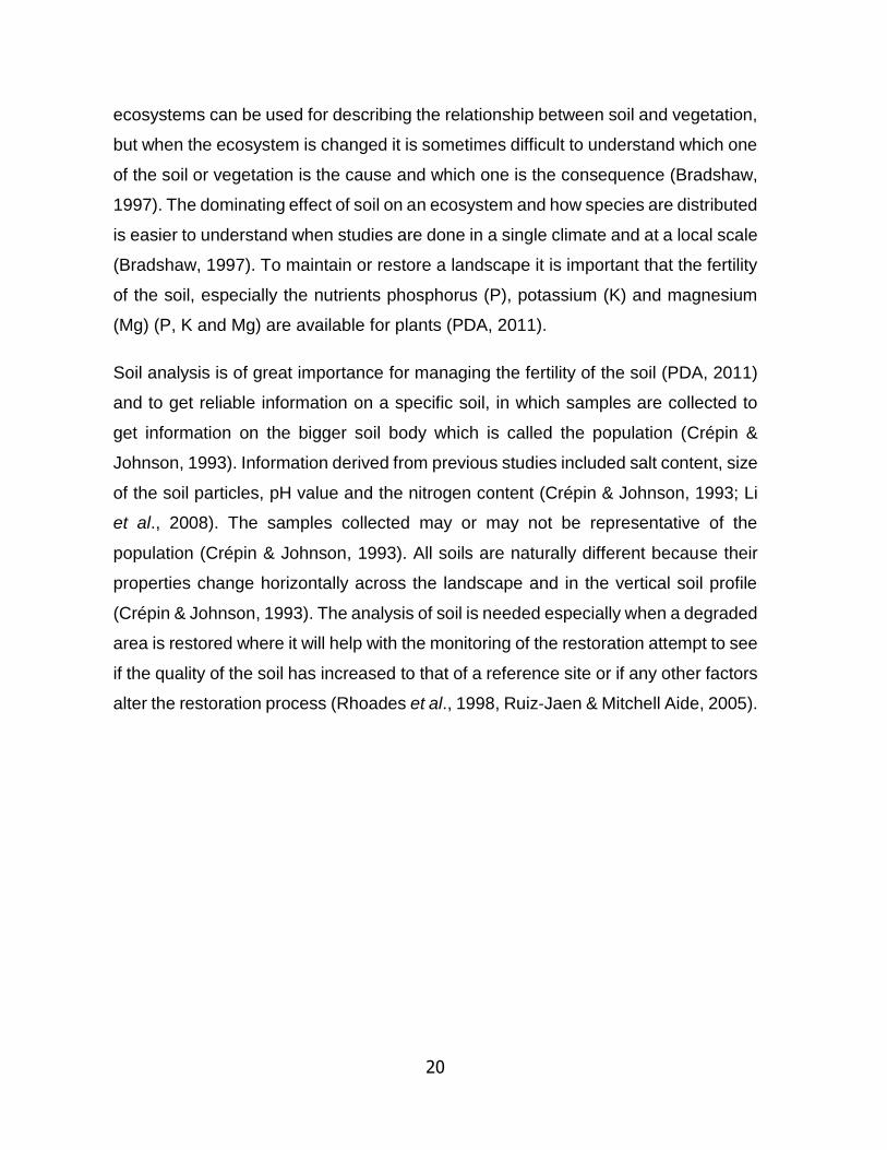


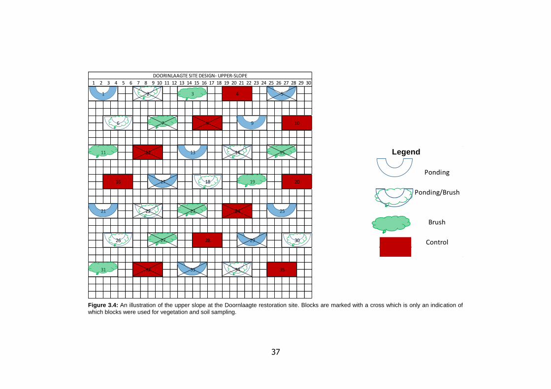
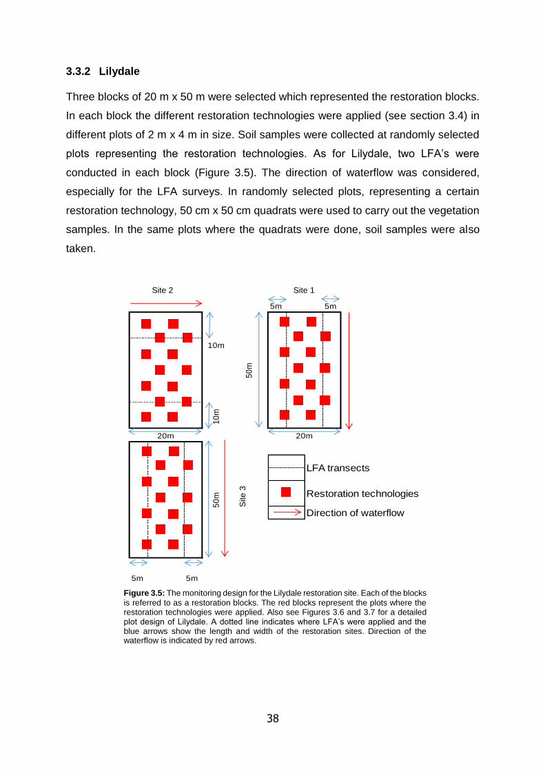


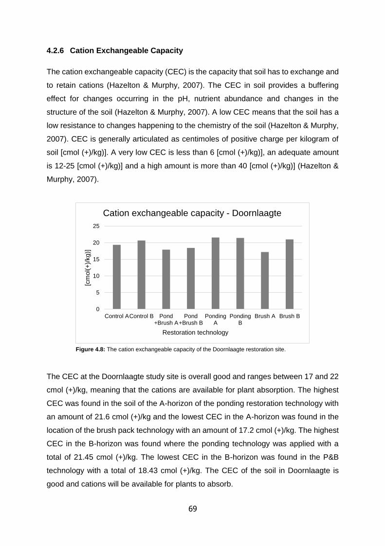


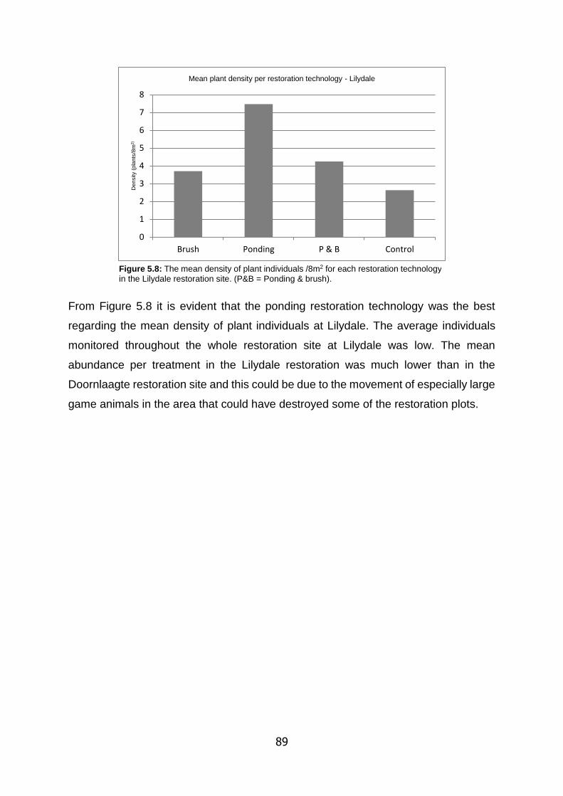


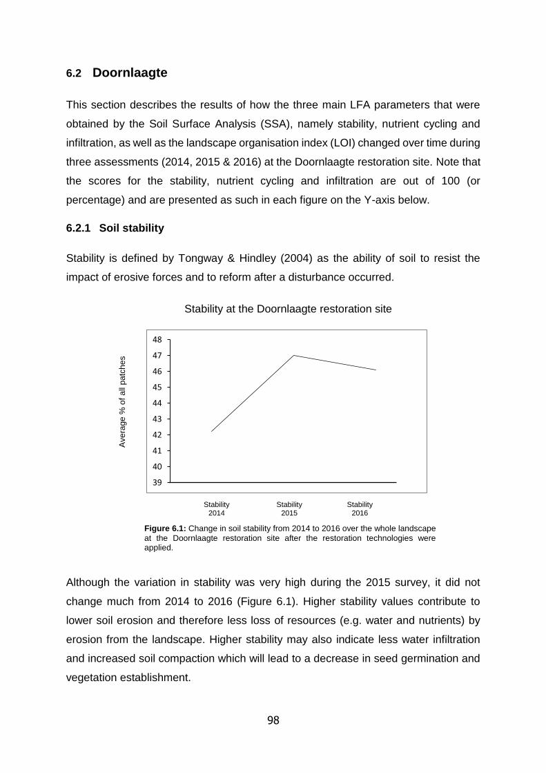


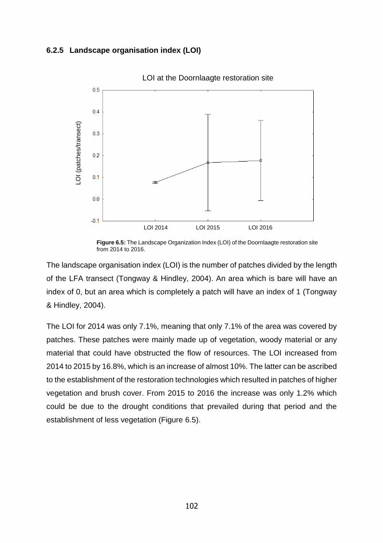


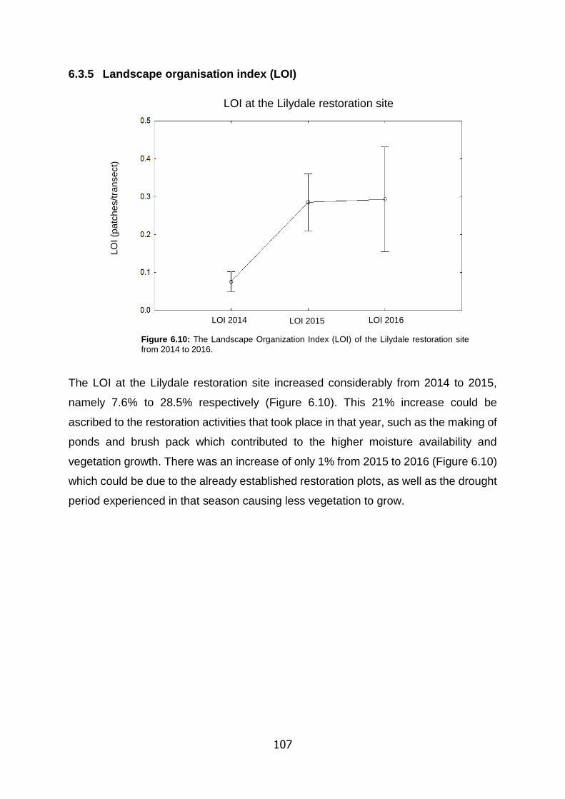


![Sustainable Restoration Technologies for Bay/Delta Tidal ...1].pdf · Sustainable Restoration Technologies for Bay/Delta Tidal Marsh and Riparian Habitat Project Information 1. Proposal](https://static.documents.pub/doc/80x56/5f81bc992a787e7d7a592234/sustainable-restoration-technologies-for-baydelta-tidal-1pdf-sustainable.jpg)


