Two-photon correlated beams, generated by spontaneousparametric downconversion in nonlinear crystals, havebeen proved largely and successfully for optical measure-ments in fields such as quantum optical communica-tion,1–4 quantum radiometry,5–13 and, more recently,quantum cryptography.14–18 Furthermore, basic experi-mental tests on the fundaments of quantum mechanicshave been performed by exploiting the entanglement ofthis source.19–21
Due to a nonlinear interaction in a x (2) crystal, somepump photons (angular frequency vp) may spontaneouslysplit into lower-frequency pairs of photons, historicallycalled signal (s) and idler (i), perfectly correlated in all as-pects of their state (direction, energy, and polarization,e.g., with angular frequency vs and v i , under the con-straints of conservation of energy and wave-vector mo-mentum, otherwise known as phase matching).
A typical general scheme for the above-mentioned opti-cal measurements is depicted in Fig. 1. With phase-matching rules,22 signal and idler pairs can be emittednoncollinearly with the pump, making for easy opticaldiscrimination of signal and idler quantum channels inthe nondegenerate case. This scheme eventually lends tothe absolute measurement of quantum efficiency, h, andtransmittance, t, by use of a channel as a trigger or ref-erence (idler, i) and the other channel as a probe or chan-nel under test (CUT) (signal, s). A more complicated butbasically similar scheme is employed in quantum commu-nication and quantum-cryptography key distribution. Adetailed analysis is beyond the aim of this paper, as werestrict ourselves to exploring the main practical limita-tions in the general case.
Basically, the underlying feature of these measure-ments relies on the realization of two quantum correlatedoptical channels yielding essentially single-photon statestriggering on one photon of the pair and counting theother in coincidence. This simple statement leads to theobvious consideration that two-photon correlated beamsbring noise reduction with respect to a single beam,23 but
this argument must be softened for the triggering (refer-ence) photons are randomly distributed, and their ownnoise fluctuation enters in the evaluation of the overallnoise in the two-photon-based measurements.
Contributions to statistical noise24,25 in a real experi-mental setup are herein investigated and modeled withthe aim of evaluating the ultimate practical uncertaintyand accuracy limit. Some systematic effects for radio-metric applications have been fully discussed else-where.13,26
To distinguish between the optical paths of correlatedphotons, interference filters with different bandwidthsand diaphragms are properly matched; they select alsounwanted uncorrelated photons due to spontaneous para-metric downconversion itself, resulting in an increaseddegree of uncorrelation, noise fluctuation in coincidencemeasurements, and asymmetry between the two chan-nels, whose mean photon rate can be quite different.This last aspect is particularly worth mentioning in thecase of radiometric applications since accuracy imposescapture in the probe channel of at least the same amountof correlated photons present on the trigger channel.13,26
Let axrx with x 5 s, i, indicating the mean rate of cor-related photons in the signal and idler channels (0 , ax, 1). The terms (1 2 ax)rx take into account also ad-ditive background photon rates due to stray light and de-tector noise. We address the total mean photon rate inchannel x as
rx 5 axrx 1 ~1 2 ax!rx ,
where we consider also the case of different levels of cor-relation as Þ a i , and asrs 5 a ir i are the same correlatedphoton rates.
Actually, statistical noise is also due to losses of corre-lated photons for the presence of optical elements, non-ideal detectors, and electronic devices in either channel.The random nature of loss mechanisms induces an in-creasing noise in the coincidence measurement due to thedistortion of the intrinsic quantum statistics of correlatedphotons. We distinguish therefore between optical losses(transmittance of the correlated photon path, tx , 1), de-
2002 Optical Society of America
1248 J. Opt. Soc. Am. B/Vol. 19, No. 6 /June 2002 Castelletto et al.
tection losses (detector quantum efficiency hx , 1), andelectronic losses associated with the presence of deadtimes, during which the detection system is unable todetect photons, i.e., Dx Þ 0. Dead times are identifiedas nonextending and extending: In the first case, allphotons following a revealed photon within the fixed timeinterval Dx are ignored, and in the second case, any in-coming photon produces or prolongs Dx . Eventually,noise in measuring coincidence counts is introduced bythe finite duration of the time-coincidence window w to-gether with the presence of uncorrelated events in bothchannels.
In Section 2 a general model is thoroughly described,and statistics of true and accidental coincidences, andconsequently of total coincidences, are determined whenall those noise contributions are taken into account.10
As to the estimation problem, quantum efficiency(Section 3) and transmittance (Section 4) are treated interms of both maximum-likelihood and heuristic estima-tors, the latter deduced from experimental consider-ations, and their estimates are compared. Moreover,in Section 3, theoretical predictions of the relative noisefluctuation in quantum efficiency are comparedwith some experimental outcomes, and the two-photon-based measurement is shown to exhibit a noise lowerthan in a single-beam configuration, when correlationis not degraded too heavily by a loss mechanism.In Section 5 the presented theory is applied to theevaluation of the quantum bit-error rate (QBER) in asimple scheme of quantum-cryptography key distribu-tion.
2. STATISTICS OF COINCIDENCES: AGENERAL MODELWe build up a model to obtain the probability distributionof coincidence mc in a time T, when all noise contribu-tions are taken into account. First, we start with thecase of ideal electronics where dead times Ds 5 Di 5 0,and we also neglect the presence of a coincidence window(w 5 0) and optical losses in the idler channel (t i 5 1).The distribution probability of photon number n in chan-nel x obeys a Poissonian law, Px(n) 5 (rxT)n
3 exp(2rxT)/n!, as well as the distribution probability ofcorrelated photons na , P(na) 5 (axrxT)na
3 exp(2axrxT)/na!. The probability distribution of ma
correlated counts in channel x is still Poissonian,27
where B(m,n, p) 5 ( mn )pm(1 2 p)n2m is a binomial dis-
tribution. We calculate also the probability of measuringcoincidence mc in the presence of ts and hs for the signalchannel as the following convolution:
P~mc! 5 (ma5mc
`
Pi~ma!B~ma , mc , tshs!
5~tshsa ir it ih iT !mc
mc!exp~2tshsa ir ih it iT !. (2)
In a general model, Ds Þ Di Þ 0 due to both detectorsand electronics, and the presence of the temporal-coincidence window w modifies the distribution probabil-ity of coincidence counts, thus leading to distinction be-tween true and accidental coincidence statistics. In thefollowing, P(m) will denote the general probability distri-bution whenever dead-time distortions lead to probabilitydistributions different from Poissonian P(m).
To obtain the statistics of true coincidences we first cal-culate the probability distribution of ma8 correlated eventsin the x channel, Px
ext(ma8 ), for the case of extending deadtime according to Eq. (1) as
Pxext~ma8 ! 5 (
ma5ma8
`
Px~ma!B~ma , ma8 , pxext! 5 Px~ma8 !,
(3)
where Px(ma8 ) 5 (axrxhxtxpxextT)ma8 exp(2axrxhxtxpx
extT)/ma8 !, and px
ext 5 exp(2rxhxtxDx). Note that Px(ma8 ) isstill Poissonian. In the case of nonextending dead time,
Pxnext~ma8 ! 5 Px~ma8 , axrxhxtxT, Dx!
5 g@ma8 ;axrxhxtx~T 2 ma8Dx!#/~ma8 2 1 !!
2 g$ma8 1 1;axrxhxtx
3 @T 2 ~ma8 1 1 !Dx#%/ma8 ! (4)
turns out to be a combination of incomplete gammafunctions,28 g@ma8 ;axrxhxtx(T 2 ma8Dx)#.27 The prob-ability distribution of true coincidence, P (c)(mc8), is evalu-ated according to Eq. (2):
P ~c !~mc8! . (ma85mc8
`
Pi~ma8 !B~ma8 , mc8 , tshsps* !, (5)
where px* 5 pxext in the extending dead-time case, and
px* 5 1/(1 1 rxhxtxDx) is the approximated correctionto the mean rate in the nonextending case. px
ext and pxnext
coincide at the first order of the series expansionin rxhxtxDx ! 1. Observe that, so far, indexes s and ican be interchanged because of the symmetry of cor-related channels. The calculable extending caseproduces for Eq. (5) a Poissonian distribution P (c)(mc8)5 (tshsps
extp iexta ir ih it iT)mc8 exp(2tshsps
extp iexta ir ih it iT)/
Castelletto et al. Vol. 19, No. 6 /June 2002 /J. Opt. Soc. Am. B 1249
mc8!, whereas the nonextending dead-time case cannot beanalytically expressed and only numerical calculationsare possible.
As to accidental coincidences, they are due to either (a)uncorrelated events that randomly contribute to coinci-dence counts or (b) events occurring on one channel aris-ing from correlated photons fortuitously coincident withuncorrelated events on the other channel, when theirtwin photons have been canceled out by a loss mecha-nism.
In channel i the mean rate for events of type (a) is(1 2 a i)r ih it i , and for events of type (b), a ir ih it i(12 hstsps* ) result, when Di 5 0. The total mean rates ofthe events in the idler and signal channels yielding acci-dental counts are then
rR,i 5 r ih it i~1 2 a ihstsps* !,
rR,s 5 rshsts~1 2 ash it ip i* !. (6)
These results allow the same formalism of Eq. (3) to beapplied for deriving the probability to count mR8 events inchannel i when Di Þ 0. From the probability P(mR)5 (rR, iT)mR exp(2rR, iT)/mR! for counting mR events po-tentially contributing to accidental coincidence, we conse-quently deduce the probability to count mR8 events accord-ing to Eq. (3) as
Pi~mR8 , rR,iT, Di! ' (mR5mR8
`
P~mR!B~mR , mR8 , p i* !.
(7)
Forwardly, the idler channel definitely plays the role ofthe trigger; thus the signal and idler cannot be inter-changed anymore, even though the same argumentstreated for the idler can be reversed to the signal as well.To evaluate the distribution probability of accidental co-incidence, we calculate the probability that uncorrelatedevents on channel s occurred in the coincidence temporalwindow, w, as
ps 5 (mR8 51
`
Ps~mR8 , rR,sw, Ds!, (8)
where we extended to channel s the arguments leading toEq. (7).
In the case of an extending dead time, Eq. (7) gives aPoissonian distribution, Pi(mR8 , rR,iT, Di) 5 P(mR8 )5 (rR,ip i
extT)mR8 exp(2rR,ipiextT)/mR8 !, and ps 5 1
2 exp(2rR,swpsext). It is easy to understand that pi
Þ ps and that from this point on the two channels cannoteven be interchanged.
Finally, the probability distribution of accidentalcounts is calculated again by applying Eq. (3),
Pi~a !~ma! 5 (
mR8 5ma
`
Pi~mR8 , rR,iT, Di!B~mR8 , ma , ps!,
(9)
which, in the case of extending dead time, still exhibits aPoissonian distribution, P i
(a)(ma) 5 exp(2rR,iTpiextps)
3 (rR,iTp iextps)
ma/ma!.
The distribution probability of total coincidence countscorresponding to Eq. (2) is then
Pi~mc! 5 (ma50
`
(mc850
`
dmc , ma 1 mc8Pi
~a !~ma!P ~c !~mc8!.
(10)
Then the optimal estimator for any parameter, y, involvedin the distribution probability, i.e., the maximum-likelihood (ML) best estimator, yML , can be calculatedfrom Eq. (10), by maximizing the probability distribution,in respect to
]P~mc!
]y5 0. (11)
Its relative noise fluctuation (relative statistical uncer-tainty) is defined as
eR~ yML! 5 S ^yML2 & 2 ^yML&2
^yML&2 D 1/2
, (12)
where ^yMLk & 5 Smc50
` P(mc) yMLk are the moments of the
estimator.In the next sections we discuss the application of the
presented theory for estimating measurands such asquantum efficiency and transmittance and their statisti-cal uncertainty in typical experiments performed so far.
3. QUANTUM EFFICIENCYThe quantum efficiency of the detection system, hsps ,i.e., the quantum efficiency of the device under test with-out dead-time correction, has been measured by sponta-neous parametric downconversion by several groups.5,7–13
It is at the moment a challenge in the realm of primaryradiometric standards, since its exploitation might sur-pass the actual drawbacks of presently available methodsfor absolute realization and dissemination, based on long,complicated, and costly hierarchical chains tracing backto national primary standards. To establish the feasibil-ity of an uncertainty level lower than that so far demon-strated, a proper estimate is required for the quantum ef-ficiency, together with the associated ultimate limit noise.
We measured the quantum efficiency with the arrange-ment illustrated in Fig. 1. An argon-ion laser (vp) pro-duces the vertically polarized 351.2-nm pump beam di-rected into a nonlinear crystal (NLC), LiIO3 , 10 mm3 10 mm 3 5 mm.
We selected two channels, corresponding to signal andidler photons, respectively, directed to two photoncounters. The trigger channel selects a short range ofwavelengths, defined by a diaphragm and a narrow inter-ference filter, whereas the signal channel (CUT) isbroader, to ensure that all photons correlated with thosearriving at the trigger fall on the CUT. We emphasizethat, although this item is crucial to the accuracy of theentire technique,26 here we consider only those param-eters that increase statistical noise in coincidence mea-surements.
Both trigger and CUT detectors were single-photonmodules equipped with active-quenching circuits. Thetrigger detector is a single-photon avalanche photodiode
1250 J. Opt. Soc. Am. B/Vol. 19, No. 6 /June 2002 Castelletto et al.
with a 180-mm-diameter sensitive area. This detector isa module coupled to a short-length multimode optical fi-ber by a lens integrated within the detector. The triggeris equipped with an interference filter, peaked at 789 nmwith 3-nm FWHM, and an iris Ii , of 4-mm diameter and 2m from the parametric-downconversion source. We cali-brated two different avalanche photodiodes on the CUT:DUT (device under test) A, with a sensitive area of500-mm diameter, and DUT B, a fiber-coupled avalanchephotodiode identical to the trigger detector. A and B areequipped with two different interference filters, bothpeaked at 633 nm with 10-nm FWHM, and an identicaliris Is with 4-mm diameter and 1 m from the parametric-downconversion source.
Coincidences and single counts were measured by atime-to-amplitude converter circuit that measures timeintervals between the photon (pulse) arrivals in the twochannels and generates a pulse with an amplitude pro-portional to their time separation. Dead times weremeasured separately for time-to-amplitude convertersand detectors.
Experimental conditions for the calibration of the twodetectors were almost the same (identical values ofh i 5 0.534, t i 5 0.586, Di 5 1600 ns, w 5 3.9 ns, andT 5 10 s) except for different values of r i , rs /r i , and a i .
In general, measurands should be estimated by an op-timal estimation providing the minimum uncertainty aswell as a meaningful estimate. Robustness is ensuredonly when a physical law describing the whole measure-ment process is available, as it is in this case. Neverthe-less, some estimators based on an oversimplified and non-statistical estimation model corrected for systematicerrors (here referred to as the heuristic model) are consid-ered erroneously robust and optimal and are used some-times. Furthermore, uncertainty is generally treated asa task independent from the estimate of the measurand,although the two problems are intimately connected, be-ing the two faces of a more general estimation problem.
In the following we develop two estimation models, themaximum-likelihood (ML) estimator and the heuristicone. We apply them to the analysis of experimental re-sults.
A. Maximum-Likelihood Best Estimator hsp sML andNoise LimitThe maximum-likelihood best estimator and its relativeuncertainty are calculated by Eqs. (11) and (12). For anextending dead time, Eq. (10) is directly a Poissonian dis-tribution, given by Pi(mc) 5 exp(2rc,iT) (rc,iT)mc/mc!and rc,i 5 r ih it ip i
ext 2 p iextrR,i exp(2rR,sps
extw). A quitegood approximation for nonextending dead time is simplyperformed by supposing that its distortion effect involvesonly the mean value, thus neglecting the presence of sub-Poissonian statistics and therefore allowing us to writePi(mc) ' Pi(mc), whose mean rate is rc,i 5 r ih it ip i
next
2 p inextrR,i exp(2rR,sps
nextw).The maximum-likelihood best estimator is therefore
determined simply by solving
rc,iT 2 mc 5 0. (13)
In this case the maximum-likelihood best estimator is cal-culated at the first perturbative order of Eq. (13), deriving
hsp sML 'mc
tsa ir ih ip i* t iT@1 1 r iw~as21 2 h it ip i* !#
.
(14)
The associated relative noise fluctuation is
eR~hsp sML! 5 ^mc&21/2
' $T^hsp s&r ih ip i* t itsa i
3 @1 1 wr i~h it ip i* 2 as21!
3 ~a its^hsp s& 2 1 !#%21/2. (15)
Equations (14) and (15) hold exactly for the extendingdead time, where p i* 5 p i
ext , and approximately for thenonextending dead time, where p i* 5 p i
next .Table 1 reports the estimate hsp sML and its associated
statistical noise, eR(hsp sML), for DUT A and DUT B, to-gether with the parameters availed. Note, in particular,the high dispersion of quantum efficiency for DUT A; thisresult can be here explained mainly by the very low trig-ger rate (r i in Table 1). To clarify this behavior, we ex-amined the relative noise fluctuation of the maximum-likelihood best estimator, eR(hsp sML), as a function of allthose experimental parameters degrading the correlationlevel in the coincidence measurement. These parametersare essentially distinguished as pure statistical(a i , r i , rs /r i , h i) and electronic (Di ,Ds ,w), for they in-duce different noise responses.
The lowest relative statistical uncertainty is obviouslyachieved in the ideal condition, i.e., rs /r i 5 1, high pho-ton rates, no optical losses (ts 5 t i 5 1), no detectionlosses (hs 5 h i 5 1), minimized dead time, and narrowcoincidence window. It is worth mentioning, even iftrivial, that eR(hsp sML) decreases also for increasing esti-mate values.
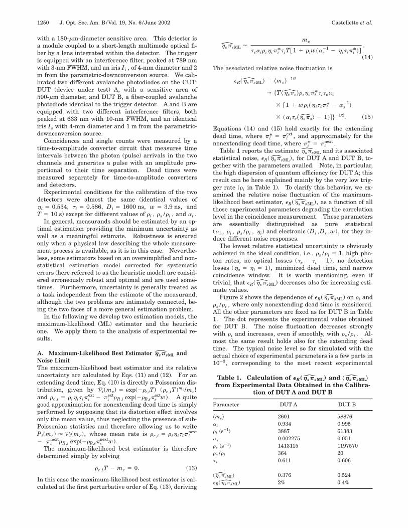
Figure 2 shows the dependence of eR(hsp sML) on r i andrs /r i , where only nonextending dead time is considered.All the other parameters are fixed as for DUT B in Table1. The dot represents the experimental value obtainedfor DUT B. The noise fluctuation decreases stronglywith r i and increases, even if smoothly, with rs /r i . Al-most the same result holds also for the extending deadtime. The typical noise level so far simulated with theactual choice of experimental parameters is a few parts in1023, corresponding to the most recent experimental
Table 1. Calculation of eR(hsp sML) and ^hsp sML&from Experimental Data Obtained in the Calibra-
tion of DUT A and DUT B
Parameter DUT A DUT B
^mc& 2601 58876a i 0.934 0.995r i (s21) 3887 61383as 0.002275 0.051rs (s21) 1413115 1197570rs /r i 364 20ts 0.611 0.606
^hsp sML& 0.376 0.524eR(hsp sML) 2% 0.4%
Castelletto et al. Vol. 19, No. 6 /June 2002 /J. Opt. Soc. Am. B 1251
performances10,13,26 as well as to the example reported inTable 1. As shown in Fig. 2 from the indication of thenoise level achieved in DUT B, we remark that these mea-surements can be improved to some respect in terms ofnoise fluctuations from 4 3 1023 to 1 3 1023, providedan optimization of the parameters (r i , rs /r i) consideredin the figure.
As to the dependence of eR(hsp sML) on a i , for typicalvalues of rs /r i 5 2, 10, and 20, the maximum ratioRMAX 5 eR(hsp sML, a i)/eR(hsp sML, a i 5 0.999) . 1.3 fora i 5 0.6, when r i 5 400 kHz and rs /r i 5 2, and theother parameters are set as in Fig. 3. In other words,noise fluctuation is significantly affected by 1 2 a i ,which, if irises are matched, is mainly due to dark countsplus stray light. Furthermore, the trigger efficiency h imay influence dramatically the noise level of the mea-surement, yielding a factor RMAX 5 eR(hsp sML, h i)/eR(hsp sML, h i 5 0.8) . 3.6 when rs /r i 5 2,r i 5 200 kHz, and h i 5 0.05.
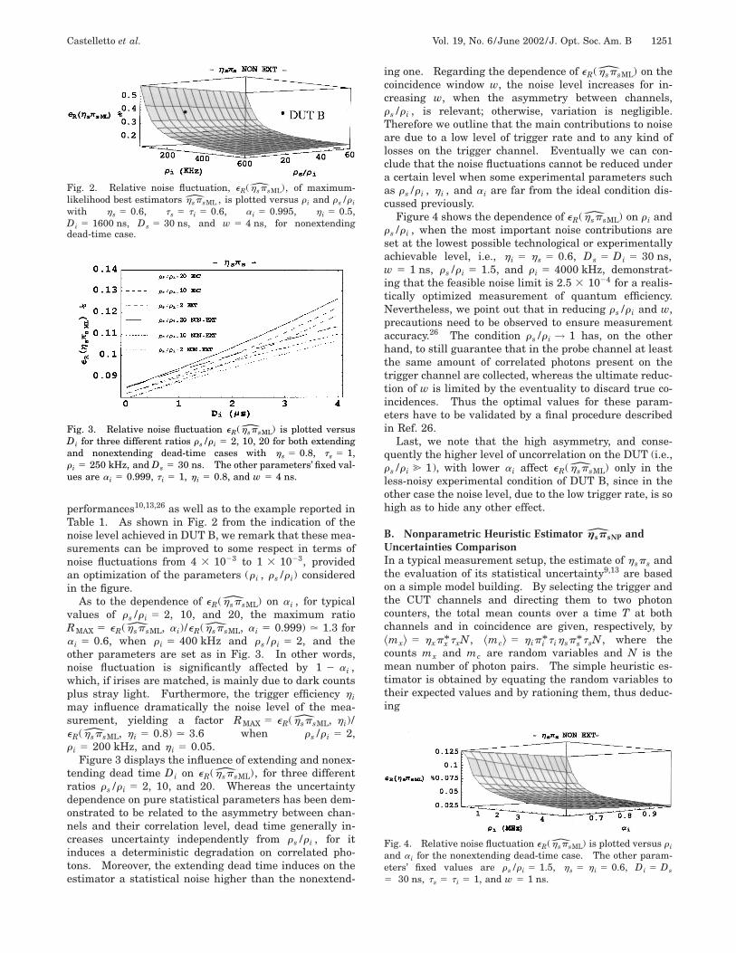
Figure 3 displays the influence of extending and nonex-tending dead time Di on eR(hsp sML), for three differentratios rs /r i 5 2, 10, and 20. Whereas the uncertaintydependence on pure statistical parameters has been dem-onstrated to be related to the asymmetry between chan-nels and their correlation level, dead time generally in-creases uncertainty independently from rs /r i , for itinduces a deterministic degradation on correlated pho-tons. Moreover, the extending dead time induces on theestimator a statistical noise higher than the nonextend-
Fig. 2. Relative noise fluctuation, eR(hsp sML), of maximum-likelihood best estimators hsp sML , is plotted versus r i and rs /r iwith hs 5 0.6, ts 5 t i 5 0.6, a i 5 0.995, h i 5 0.5,Di 5 1600 ns, Ds 5 30 ns, and w 5 4 ns, for nonextendingdead-time case.
Fig. 3. Relative noise fluctuation eR(hsp sML) is plotted versusDi for three different ratios rs /r i 5 2, 10, 20 for both extendingand nonextending dead-time cases with hs 5 0.8, ts 5 1,r i 5 250 kHz, and Ds 5 30 ns. The other parameters’ fixed val-ues are a i 5 0.999, t i 5 1, h i 5 0.8, and w 5 4 ns.
ing one. Regarding the dependence of eR(hsp sML) on thecoincidence window w, the noise level increases for in-creasing w, when the asymmetry between channels,rs /r i , is relevant; otherwise, variation is negligible.Therefore we outline that the main contributions to noiseare due to a low level of trigger rate and to any kind oflosses on the trigger channel. Eventually we can con-clude that the noise fluctuations cannot be reduced undera certain level when some experimental parameters suchas rs /r i , h i , and a i are far from the ideal condition dis-cussed previously.
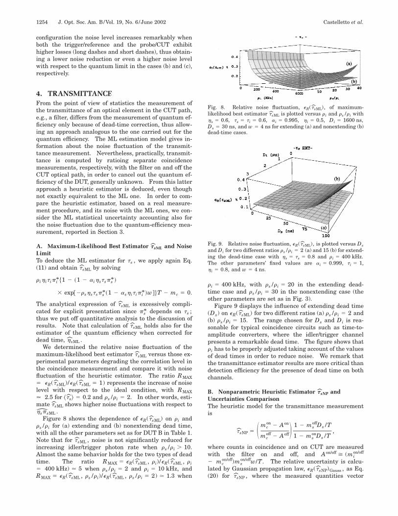
Figure 4 shows the dependence of eR(hsp sML) on r i andrs /r i , when the most important noise contributions areset at the lowest possible technological or experimentallyachievable level, i.e., h i 5 hs 5 0.6, Ds 5 Di 5 30 ns,w 5 1 ns, rs /r i 5 1.5, and r i 5 4000 kHz, demonstrat-ing that the feasible noise limit is 2.5 3 1024 for a realis-tically optimized measurement of quantum efficiency.Nevertheless, we point out that in reducing rs /r i and w,precautions need to be observed to ensure measurementaccuracy.26 The condition rs /r i → 1 has, on the otherhand, to still guarantee that in the probe channel at leastthe same amount of correlated photons present on thetrigger channel are collected, whereas the ultimate reduc-tion of w is limited by the eventuality to discard true co-incidences. Thus the optimal values for these param-eters have to be validated by a final procedure describedin Ref. 26.
Last, we note that the high asymmetry, and conse-quently the higher level of uncorrelation on the DUT (i.e.,rs /r i @ 1), with lower a i affect eR(hsp sML) only in theless-noisy experimental condition of DUT B, since in theother case the noise level, due to the low trigger rate, is sohigh as to hide any other effect.
B. Nonparametric Heuristic Estimator hsp sNP andUncertainties ComparisonIn a typical measurement setup, the estimate of hsps andthe evaluation of its statistical uncertainty9,13 are basedon a simple model building. By selecting the trigger andthe CUT channels and directing them to two photoncounters, the total mean counts over a time T at bothchannels and in coincidence are given, respectively, by^mx& 5 hxpx* txN, ^mc& 5 h ip i* t ihsps* tsN, where thecounts mx and mc are random variables and N is themean number of photon pairs. The simple heuristic es-timator is obtained by equating the random variables totheir expected values and by rationing them, thus deduc-ing
Fig. 4. Relative noise fluctuation eR(hsp sML) is plotted versus r iand a i for the nonextending dead-time case. The other param-eters’ fixed values are rs /r i 5 1.5, hs 5 h i 5 0.6, Di 5 Ds5 30 ns, ts 5 t i 5 1, and w 5 1 ns.
1252 J. Opt. Soc. Am. B/Vol. 19, No. 6 /June 2002 Castelletto et al.
hsp s 51
ts
mc
mi. (16)
The simple model in Eq. (16) is corrected for accidentalcounts as
hsp s 51
tsS mc 2 A
mi 2 mN,iD , (17)
where mc are the coincidence counts measured in thetime window w, mN,i are the background counts on thetrigger, and ts is the overall transmittance of the opticalelements in the signal channel. Accidental coincidences,
A 5 ~mi 2 mc!Fms
w
T1
1
2 S ms
w
T D 2G ,
are calculated according to Refs. 9 and 29.Actually, the signal and idler counts are affected by the
quantum efficiency of the detection system and the elec-tronics dead time, Dx , as well as by optical losses. Bysubstituting mean counts in A with ^mi& 5 r ih it ip i* T,^mN ,i& 5 (1 2 a i) r ih it ip i* T and ^ms& 5 rshstsps* T, wederive the estimator generally adopted in these experi-ments,
According to Eq. (12) the relative noise fluctuation is
eR~hsp sNP! 5 eR~hsp sML!
3 H 1 2^mc&
r ih ip i* t iT@1 1 as /~r iw !#J 21
. eR~hsp sML!, (19)
thus proving that hsp sNP is not optimal.As to the uncertainty evaluation of the nonparametric
(NP) estimate, the reasonable procedure adopted sofar9,13,26 is founded on the Gaussian uncertainty propaga-tion on Eq. (17), by considering mx and mc random vari-ables, Poissonian distributed, whose degree of correlationis easily calculable according to the general model. Therelative uncertainty for hsp sNP obtained by the Gaussianuncertainty propagation is30
eR~hsp sNP!Gauss 51
^hsp sNP&~J • C • JT!1/2, (20)
where (J) l 5 ]hsp sNP /]Xlu^X& , l 5 1, 4, is the Jacobianvector calculated on the expected values of XT
5 (mcmimsmN,i), the vector of measured quantities, andC is the variance–covariance matrix, here explicitly cal-culated as31
C 5 F ^mc& ^mc& ^mc& ^ms&^mN,i&w/T
¯ ^mi& ^mc& ^mN,i&
¯ ¯ ^ms& ^ms&^mN,i&w/T
¯ ¯ ¯ ^mN,i&
G .
Nonparametric and maximum-likelihood best estima-tors for hsp s are computed with corresponding uncertain-ties in case of nonextending dead time. Results are com-pared in conditions far from the ideal ones of equalchannels, adopting reasonable parameters as for simula-tions in Subsection 3.A. The relative noise fluctuation,eR(hsp sML) and eR(hsp sNP), can be regarded as equalwith a maximum discrepancy of 4 3 1024 at a 0.3% levelof relative noise, when rs /r i 5 1, hs 5 h i 5 0.8,r i 5 250 kHz, Di 5 1600 ns, Ds 5 30 ns, and t i 5 ts5 1. Results on eR(hsp sML), eR(hsp sNP), andeR(hsp sNP)Gauss are reported in Table 2 for the experimen-tal conditions of Table 1, thus confirming that ML is theoptimal estimator but stating that, when the experimen-tal conditions are far from the ideal ones, the uncertaintyof the ML estimator is definitely equivalent to the NP one.Note that eR(hsp sNP)Gauss is lower than ML and NP inboth cases. This behavior is analyzed in detail below.
The relative discrepancy between NP and ML esti-mates, DR(hsp s) 5 (^hsp sML& 2 ^hsp sNP&)/^hsp sML&, is
negligible when all parameters are set approximately inthe experimental conditions for DUT B in Table 1, withrs /r i 5 1.5, h i 5 0.6, ts 5 t i 5 1, and a i 5 0.999, yield-ing a noise level of a few parts in 1023.
However, in Fig. 5, DR(hsp s) is plotted (straight line)versus the trigger rate r i for low dead times and high pho-ton rates as in Fig. 4. In this case it is remarkable thatthe NP estimator differs from the ML one by more than5 3 1024 for r i . 2 MHz. This means that when the ex-perimental conditions are as close as possible to the idealcase and uncertainty is reduced to !0.1%, attention mustbe paid to the estimator adopted because NP may differfrom ML at a comparable uncertainty level. Further-more, eR(hsp sML) (dashes) and eR(hsp sNP)Gauss (dots) arealso plotted in Fig. 5, showing that eR(hsp sML). eR(hsp sNP)Gauss , as is clear also from the calculations
hsp sNP 'mc
tsa ir ih ip i* t iT$1 1 r iw@as21 2 mc~h ip i* t ir iasT !21#%
5 hsp sML
1 1 r iw~as21 2 h it ip i* !
1 1 r iw@as21 2 mc~h ip i* t ir iasT !21#
. (18)
Table 2. Calculation of eR(hsp sML), eR(hsp sNP)and eR(hsp sNP)Gauss from Experimental Data Ob-tained in the Calibration of DUT A and DUT B
Castelletto et al. Vol. 19, No. 6 /June 2002 /J. Opt. Soc. Am. B 1253
reported in Table 2, where eR(hsp sNP)Gauss is calculatedfor the experimental parameters of Table 1.
To enforce the latter argument, eR(hsp sML) andeR(hsp sNP)Gauss are plotted in Fig. 6 versus estimate ^h s&.By approximately setting parameters as for DUT B inTable 1, it turns out eR(hsp sNP)Gauss , eR(hsp sML).Moreover, eR(hsp sNP)Gauss exhibits a nonphysical behav-ior as it slopes down fast to the 0.01% level for ^h s& → 1,whereas a flat region is expected. For the sake of com-pleteness we plot the relative statistical uncertainty cal-culated by error propagation without accounting for cor-relations, eR(hsp sNP)Gauss
uncorr , showing that sinceeR(hsp sNP)Gauss
uncorr . eR(hsp sML), the evaluation of uncer-tainty without accounting for statistical correlation, evenif not correct, yields a physically acceptable result.
C. Comparison with a Single-Channel ConfigurationWe compare the two-channel method for quantum-efficiency measurement to the conventional case of asingle-channel configuration based on a single laser beamas a photon source. A single-beam setup is based on anattenuated laser beam with mean photon rate a lr l , withPoissonian distribution P(nl8 , a lr l), and stray light anddark counts are accounted for by (1 2 a l)r l . As dis-cussed in Eq. (1), the probability distribution of detectorcounts is
Fig. 5. Relative discrepancy between estimates DR(hsp s)(straight line) and associated relative uncertainty eR(hsp sML)(dashed curve) and eR(hsp sNP)Gauss (dotted curve) are plotted ver-sus r i for rs /r i 5 1.5 in the nonextending dead-time case. Theother parameters have fixed values hs 5 h i 5 0.6, ts 5 t i5 1, a i 5 0.999, Di 5 Ds 5 30 ns, and w 5 1 ns.
uncorr (dotted curve) areplotted versus associated estimates ^h s& for rs /r i 5 1.5 in thenonextending dead-time case. The other parameters have fixedvalues h i 5 0.6, ts 5 t i 5 1, a i 5 0.999, Di 5 1600 ns, Ds5 30 ns, w 5 4 ns, r i 5 250 kHz.
Pl~ml! 5 (nl5ml
`
P~nl , r l!B~nl , ml , t lh lp l!.
Detector quantum efficiency can be estimated ratioingthe mean counts, ^ml&, to the mean number of probe pho-tons incident on the detector, ^nl&, i.e., ^h lp lML&5 ^ml&/(t l^nl&), where t l is the transmittance of the op-tical path. According to Eq. (12), we calculate the rela-tive noise fluctuations eR(h lp lML) 5 (r lt lh lp lT)21/2.The underlying feature of the single-beam setup, leadingto unavoidable separate measurements of ml and nl , isthe identity between the role of the probe and the refer-ence, whereas in the two-photon scheme the absolute cali-bration avails of a channel as reference and the otherchannel as probe.32 We therefore spell out that in bothcases we focus our analysis on the basic argument that, inphoton counting, the reference also presents its ownquantum and statistical noise, which adds to the othercontributions, making this approach slightly differentfrom hitherto presented ones.7,24,33 For this reason theoverall statistical uncertainty, eR(h lp l)total , is obtained bysimply adding to eR
2 (h lp lML) the intrinsic quantum noiseof the reference (the beam itself) accounting also for thepresence of dark counts and stray light, (r lT)21, yielding
eR~h lp l!total 5 F1 1 h lh lp l
t lh lp lr lTG1/2
. (21)
In Fig. 7 we plot eR(h lp l)total as a function of referencecounts together with the relative uncertainty eR(hsp sML)in the case of the two-photon setup [Eq. (15)] for differentnoise conditions on the trigger channel. Particularly, weconsider for eR(hsp sML) (a) the lowest noise conditions(straight line), (b) a realistic configuration for noise inboth trigger and reference channels (long-dashed curve)and (c) a configuration similar to (b) with a lower triggerquantum efficiency (short-dashed curve). It is clear that,for achievable low-loss experimental conditions (a), thetwo-photon configuration allows measurement (straightline) well below the quantum noise limit given byeR(h lp l)total (dotted curve). However, in the two-photon
Fig. 7. Relative uncertainties eR(hsp sML) in the following con-ditions: rs /r i 5 1, h i 5 0.6, a i 5 1, Di 5 30 ns, and w 5 1 ns(straight line), rs /r i 5 10, h i 5 0.6, a i 5 0.96, Di 5 1600 ns,w 5 4 ns [long-dashed curve (b)], rs /r i 5 10, h i 5 0.4,a i 5 0.96, Di 5 1600 ns, w 5 4 ns [short-dashed curve (c)], to-gether with eR(h lp l)total for h l 5 hs 5 0.6, t l 5 ts 5 1, Dl 5 Ds5 30 ns (dotted curve), are plotted versus the reference/triggercounts.
1254 J. Opt. Soc. Am. B/Vol. 19, No. 6 /June 2002 Castelletto et al.
configuration the noise level increases remarkably whenboth the trigger/reference and the probe/CUT exhibithigher losses (long dashes and short dashes), thus obtain-ing a lower noise reduction or even a higher noise levelwith respect to the quantum limit in the cases (b) and (c),respectively.
4. TRANSMITTANCEFrom the point of view of statistics the measurement ofthe transmittance of an optical element in the CUT path,e.g., a filter, differs from the measurement of quantum ef-ficiency only because of dead-time correction, thus allow-ing an approach analogous to the one carried out for thequantum efficiency. The ML estimation model gives in-formation about the noise fluctuation of the transmit-tance measurement. Nevertheless, practically, transmit-tance is computed by ratioing separate coincidencemeasurements, respectively, with the filter on and off theCUT optical path, in order to cancel out the quantum ef-ficiency of the DUT, generally unknown. From this latterapproach a heuristic estimator is deduced, even thoughnot exactly equivalent to the ML one. In order to com-pare the heuristic estimator, based on a real measure-ment procedure, and its noise with the ML ones, we con-sider the ML statistical uncertainty accounting also forthe noise fluctuation due to the quantum-efficiency mea-surement, reported in Section 3.
A. Maximum-Likelihood Best Estimator t sML and NoiseLimitTo deduce the ML estimator for ts , we apply again Eq.(11) and obtain t sML by solving
r ih it ip i* $1 2 ~1 2 a ihstsps* !
3 exp@2rshstsps* ~1 2 ash it ip i* !w#%T 2 mc 5 0.
The analytical expression of t sML is excessively compli-cated for explicit presentation since ps* depends on ts ;thus we put off quantitative analysis to the discussion ofresults. Note that calculation of t sML holds also for theestimator of the quantum efficiency when corrected fordead time, h sML .
We determined the relative noise fluctuation of themaximum-likelihood best estimator t sML versus those ex-perimental parameters degrading the correlation level inthe coincidence measurement and compare it with noisefluctuation of the heuristic estimator. The ratio RMAX5 eR(t sML)/eR(t sML 5 1) represents the increase of noiselevel with respect to the ideal condition, with RMAX. 2.5 for ^t s& 5 0.2 and rs /r i 5 2. In other words, esti-mate t sML shows higher noise fluctuations with respect tohsp sML .
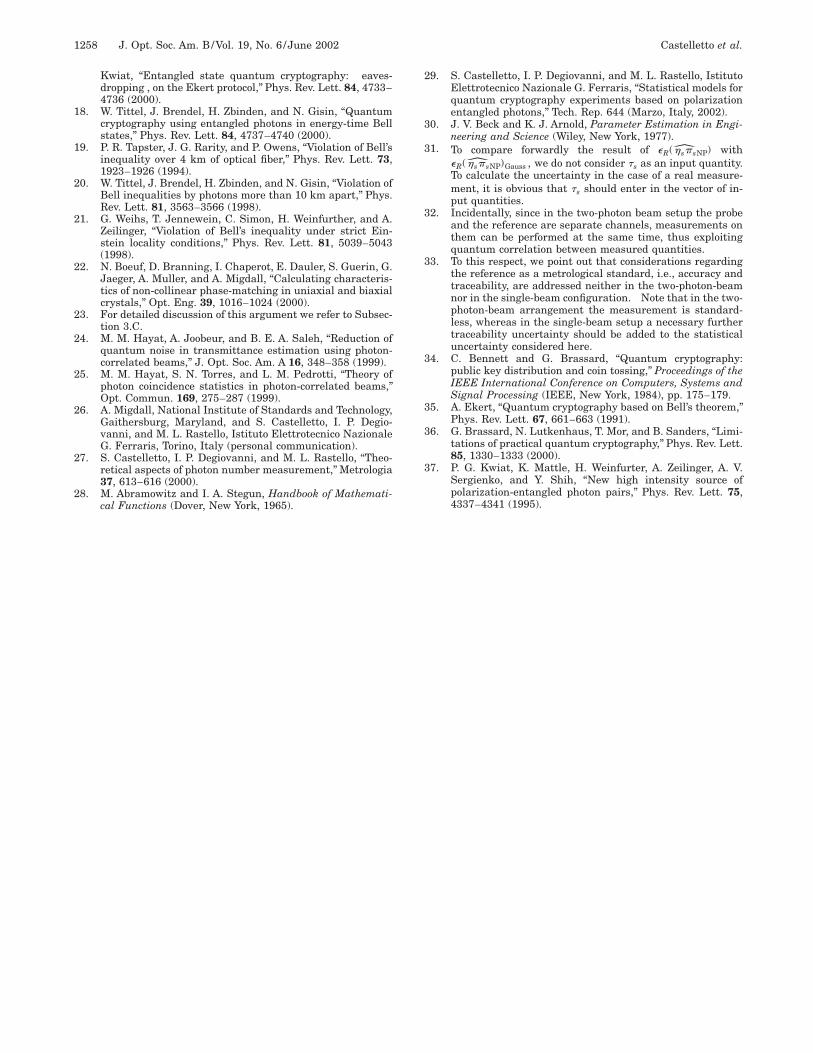
Figure 8 shows the dependence of eR(t sML) on r i andrs /r i for (a) extending and (b) nonextending dead time,with all the other parameters set as for DUT B in Table 1.Note that for t sML , noise is not significantly reduced forincreasing idler/trigger photon rate when rs /r i . 10.Almost the same behavior holds for the two types of deadtime. The ratio RMAX 5 eR(t sML , r i)/eR(t sML , r i5 400 kHz) . 5 when rs /r i 5 2 and r i 5 10 kHz, andRMAX 5 eR(t sML , rs /r i)/eR(t sML , rs /r i 5 2) . 1.3 when
r i 5 400 kHz, with rs /r i 5 20 in the extending dead-time case and rs /r i 5 30 in the nonextending case (theother parameters are set as in Fig. 3).
Figure 9 displays the influence of extending dead time(Dx) on eR(t sML) for two different ratios (a) rs /r i 5 2 and(b) rs /r i 5 15. The range chosen for Ds and Di is rea-sonable for typical coincidence circuits such as time-to-amplitude converters, where the idler/trigger channelpresents a remarkable dead time. The figure shows thatr i has to be properly adjusted taking account of the valuesof dead times in order to reduce noise. We remark thatthe transmittance estimator results are more critical thandetection efficiency for the presence of dead time on bothchannels.
B. Nonparametric Heuristic Estimator t sNP andUncertainties ComparisonThe heuristic model for the transmittance measurementis
t sNP 5 S mcon 2 Aon
mcoff 2 AoffD 1 2 ms
offDs /T
1 2 msonDs /T
,
where counts in coincidence and on CUT are measuredwith the filter on and off, and Aon/off > (mi
on/off
2 mcon/off)ms
on/offw/T. The relative uncertainty is calcu-lated by Gaussian propagation law, eR(t sNP)Gauss , as Eq.(20) for t sNP , where the measured quantities vector
Fig. 8. Relative noise fluctuation, eR(t sML), of maximum-likelihood best estimator t sML is plotted versus r i and rs /r i withhs 5 0.6, ts 5 t i 5 0.6, a i 5 0.995, h i 5 0.5, Di 5 1600 ns,Ds 5 30 ns, and w 5 4 ns for extending (a) and nonextending (b)dead-time cases.
Fig. 9. Relative noise fluctuation, eR(t sML), is plotted versus Dsand Di for two different ratios rs /r i 5 2 (a) and 15 (b) for extend-ing the dead-time case with hs 5 ts 5 0.8 and r i 5 400 kHz.The other parameters’ fixed values are a i 5 0.999, t i 5 1,h i 5 0.8, and w 5 4 ns.
Castelletto et al. Vol. 19, No. 6 /June 2002 /J. Opt. Soc. Am. B 1255
XT 5 (mcon mi
on mson mc
off mioff ms
off), and the variance–covariance is a 6 3 6 matrix, here explicitly calculated as
C 5 FCon 0
0 CoffG ,with
Cx 5 F ^mc&x ^mc&
x ^mc&x
¯ ^mi&x ^mc&
x
¯ ¯ ^ms&xG ,
where x indicates the on/off condition on the filter.As for the quantum efficiency, we compare the nonpara-
metric and the maximum-likelihood best estimators fort s, by adopting parameters as previously. With this pur-pose we consider the total relative noise fluctuation fort sML as eR(t sML)total 5 @eR
2 (t sML) 1 eR2 (h sML)#1/2, where
eR2 (h sML) is the relative uncertainty associated with the
detector calibration calculated by the ML model in Eq.(15). We emphasize that in this case ML and NP estima-tors represent two quite different measuring approaches,so this analysis can be better considered as a comparisonbetween different methods. Even if ML is an optimalmethod, however, the NP is easier to implement practi-cally for it does not require a preliminary quantum-efficiency calibration.
In Fig. 10 the relative discrepancy between ML and NPestimates, DR(t s) 5 (^t sML& 2 ^t sNP&)/^t sML&, is shown asa function of the trigger rate for low dead times and highphoton rates (as in Fig. 4). We make special mentionthat the NP estimate differs from the ML one by morethan 5 3 1024 only for r i . 3 MHz, whereas at the 0.1%noise level this discrepancy is negligible.
In Fig. 10 we plot also eR(t sML), eR(t sML)total , andeR(t sNP)Gauss , showing the reasonable result eR(t sML), eR(t sNP)Gauss , even if also in this case we noticeeR(t sML)total . eR(t sNP)Gauss for r i . 3.5 MHz. In thecase of the noise level at 0.1%, eR(t sML)total. eR(t sNP)Gauss for r i . 100 kHz.
Fig. 10. Relative discrepancy between estimates DR(t s)(straight line) and associated relative uncertainty eR(t sML)(short-dashed curve), eR(t sML)total (dashed curve), andeR(t sNP)Gauss (dotted curve) are plotted versus r i for rs /r i 5 1.5in the nonextending dead-time case. The other parametershave fixed values hs 5 h i 5 0.8, ts 5 0.5, t i 5 1, a i 5 0.999,Di 5 Ds 5 30 ns, and w 5 1 ns.
5. QUANTUM-BIT-ERROR RATEThe here-proposed method can be successfully applied toevaluate a priori the robustness of a quantum-cryptography key (QCK) distribution against eavesdrop-ping attacks. QCK distribution, the most advanced andchallenging application of the new field of quantum infor-mation theory, offers the possibility that two remote par-ties, sender and receiver (conventionally called Alice andBob), exchange a secret key, called a sifted key (string ofqubits), to implement a secure encryption algorithm. Ina QCK distribution, Alice and Bob use a quantum chan-nel, along which sequences of signals are sent/measuredat random between two bases of orthogonal quantumstates, i.e., one corresponding to horizontal and verticallinear polarization (%), and the other to linear polariza-tions rotated by 45° (^). Alice can play the role of eithersetting randomly the polarization basis of photons andsend them to Bob (faint laser pulses as photons source) ormeasuring photons randomly in any one of the two bases(entangled-photon source). Bob, randomly and indepen-dently from Alice, measures in one of the two bases, either% or ^. The sifted key consists of the subset of measure-ments performed when the Alice and Bob chosen bases co-incide, obtaining at this point a deterministic outcome.Since they exchange the information about the basis used(but not the results of the measurement) on a classicalpublic channel and consequently they previously agree onthe correspondence between counting a photon in a spe-cific state with the value of the bit either 0 or 1, the secu-rity of the key generated relies on the laws of quantumphysics.34,35 This last claim must be somewhat softenedbecause of practical realization of quantum channels.36
Basically, QCK distribution is based on the principle that,when a third party (Eve) performs a measurement on aqubit exchanged, she induces a perturbation yielding er-rors in the bit sequence transmitted, thus revealing herpresence. Any attempt by Eve to obtain informationabout the key leads to a nonzero error rate in the gener-ated sifted key. Nevertheless, in practical systems, er-rors also happen because of experimental limits, such aslosses in optics, detection and electronics, and noise.
In order to characterize a system and to assess its ad-vantages, we evaluate the quantum bit-error rate (QBER)for a particular QCK distribution procedure, based on theentangled photons’ source. The QBER is the parameterfor describing the signal quality in transmitting the siftedkey, defined as the relative frequency of errors, i.e., thenumber of errors divided by the total size of the crypto-graphic sifted key. In other words, the probability oftransmitting m wrong bits in the sequence of K transmit-ted bits (sifted key in the specific case), for a givenQBER 5 b, is B(K, m, b) 5 (m
K )bm(1 2 b)K2m. Ac-cording to the ML estimation method, we make explicitthe estimator bML 5 m/K, whose estimate is QBER.The relative statistical uncertainty of QBER is therefore
eR~ bML! 5 S 1 2 QBER
K 3 QBERD 1/2
. (22)
As an explicit example of QBER estimation, we con-sider a very simplified version of a recently adopted opti-cal communication system16–18 for QCK distribution. By
1256 J. Opt. Soc. Am. B/Vol. 19, No. 6 /June 2002 Castelletto et al.
use of entangled photons generated by a type II paramet-ric downconversion,37 the output two-photon states resultin a quantum superposition of orthogonally polarized pho-tons in singlet states. In this respect it should be re-marked that, in the basic scheme of Fig. 1, the correlatedphotons axrx are selected also by means of their polariza-tions, i.e., by polarizing beam splitters on both arms.These entangled states show perfect correlation for polar-ization measurement along orthogonal but arbitrary axes.However, the actual outcome of an individual measure-ment on each photon is inherently random. Both thisperfect correlation as well as the random outcome fromany measurement performed on the single photon can beexploited to generate the QCK.
We consider here a simple variant of the BB84 protocol,founded on the first idea of Bennet and Brassard,34 buthere considering entangled photons, where Alice and Bob,exchanging the key, randomly vary their polarization ana-lyzers in four directions of two nonorthogonal basis (%
and ^). According to Fig. 1, we address Alice’s detectionsystem (polarization analyzer and detector) to the i chan-nel and Bob’s to the s channel. The key generation isbased on coincidence measurements between the two par-ties.
Since the directions of polarization analyzers i and sare chosen independently and randomly, only the subsetof coincidence performed with the two analyzers in thesame basis are considered to contribute to the sifted key,and the other subset is discarded; therefore the contribut-ing trigger count rate for QCK generation is 1
2r ih it ip i* .True and accidental coincidence counts obey Poissoniandistribution with mean rates, respectively,
rC8 51
4a ir ih it ip i* hstsps* , (23)
rA 51
4r ih it ip i* ps 1
1
4r ih it ip i* ps~1 2 a ihstsps* !,
(24)
where ps plays the same role as in Eq. (8) to account foraccidental coincidence, provided that rR,s is half of the ex-pression of Eq. (6). In Eqs. (23) and (24), true coinci-dences are due to the orthogonally settings of analyzers(thus only half of the trigger rate contributes), and acci-dental coincidences are present also for parallel settingsof analyzers, i.e., the first term in Eq. (24). QBER is ex-perimentally evaluated, according to the definition above,as the ratio between the contribution of the accidental co-incidences when the two analyzers are parallel and thetotal coincidences,
QBER~A ! 5^mA,i&
^mc&5
ps
2ps 2 psa ihstsps* 1 a ihstsps*,
(25)where ^mc& 5
14r ih it ip i* T(2ps 2 psa ihstsps*
1 a ihstsps* ) and ^mA,i& 514r ih it ip i* psT, if we consider
Eqs. (23) and (24). QBER 5 0.5 implies Alice and Bobhave a completely uncorrelated (a i 5 0) sequence of bits.The associated relative uncertainty is eR
(A)(bML)5 (^mA,i&
21 2 ^mc&21)1/2 ' ^mA,i&
21/2 if ^mc& @ ^mA,i&.In Fig. 11 we plot QBER(A) versus r i for rs /r i 5 1, 1.5
and a i 5 0.5, 1. Note that QBER increases with respectto r i and rs /r i , and it presents the maximum noise levelfor a i 5 0.5, corresponding to the case of a collinear con-figuration.
To test the capability of our method to evaluate thenoise level of a QCK distribution, we apply it to anotherscheme to generate the key, based only on the total corre-lation of the entangled photons. This way is more effi-cient in terms of number of bits transmitted over a cer-tain time (K) but much less efficient in terms of QBER if areal experimental setup is considered. The ideal condi-tion of absence of losses and complete correlation betweenAlice and Bob means that, for any photon detected by Al-ice, Bob extracts the key bit by checking coincidencewhose presence or absence indicates whether the analyz-ers are set orthogonal or parallel to each other, respec-tively. Nevertheless, the presence of losses introduces er-rors accounted for in QBER as follows:
QBER~B ! 5^mA,i& 1 ^mi,'& 2 ^mc,'&
^mi&
5ps 1 1 2 a ihstsps*
2, (26)
where all the trigger counts ^mi& 512r ih it ip i* T contrib-
ute to the transmission of the information. On the otherhand, errors in the sequence of bits are induced by^mi,'& 2 ^mc,'& 5
14r ih it ip i* (1 2 a ihstsps* )T, which is
Fig. 11. QBER(A) is plotted versus r i in the case of rs /r i 5 1,1.5 and a i 5 0.999,0.5. The other parameters have fixed valueshs 5 h i 5 0.8, t i 5 1, Di 5 1600 ns, Ds 5 30 ns, andw 5 4 ns.
Fig. 12. QBER(A) [(B)] is plotted versus r i in the condition (a),rs /r i 5 1, hs 5 h i 5 1, Di 5 Ds 5 w 5 1 ns dotted line[straight line], and in the realistic ones (b), rs /r i 5 1.5, hs 5 h i5 0.8, t i 5 1, a i 5 0.999, Di 5 1600 ns, Ds 5 30 ns, and w5 4 ns long-dashed line [short-dashed line], respectively. Theother parameters have fixed values a i 5 t i 5 1.
Castelletto et al. Vol. 19, No. 6 /June 2002 /J. Opt. Soc. Am. B 1257
the part of the trigger counts belonging to the subset ofthe analyzers orthogonally oriented that do not contributeto coincidence. Also in this case we report the associatedrelative uncertainty eR
(B)(bML) 5 @(^mA,i& 1 ^mi,'&2 ^mc,'&)21 2 ^mi&
21#1/2.In Fig. 12, QBER(A) and QBER(B) are plotted versus r i
in both the ideal and realistic conditions, respectively.As expected, QBER(B) . QBER(A) even when QBER(B)is calculated in the ideal conditions, thus proving the ca-pability of our method to test that the QCK distributiondeveloped according to the scheme B is inefficient interms of QBER.
6. CONCLUSIONSThis paper establishes a general model to evaluate theoverall statistical noise (uncertainty) in optical measure-ments such as detection efficiency and transmittance, aswell as QBER in a quantum-cryptography key distribu-tion system, when two-photon correlated beams gener-ated by parametric downconversion are employed. Sincethe above-mentioned experiments are essentially basedon the measurement of coincident events between corre-lated channels, the probability of coincidences is calcu-lated accounting for any noise contribution in a real ex-perimental setup, such as optical and electronics losses,considering also the random quantum nature of the trig-gering events in the experimental setups implemented sofar.
Regarding the measurement of the quantum efficiencyand transmittance, the noise fluctuation of the maximum-likelihood best estimator has been evaluated as a functionof the above-mentioned experimental parameters, anddifferent behaviors are highlighted for noise fluctuationsinduced by these losses according to their nature, purestatistical for the optical ones and deterministic for theelectronics ones. To reduce relative noise fluctuations,0.1%, trigger photons should be correlated better than99.9% and almost-equal channels should be experimen-tally realized to compensate losses introduced by real de-tectors and electronics. Aiming at reducing noise, it isrecommended to have losses and dead time as low as pos-sible in the trigger channel in order to increase thetrigger-correlated counts. The feasible lower noise levelfor quantum-efficiency measurement is estimated at;2.5 3 1024.
We compared the maximum-likelihood (ML) best esti-mators for the detection efficiency and transmittance withthe nonparametric (NP) heuristic ones, which are gener-ally more likely employable in experiments. When ex-perimental arrangements lead to a noise level of someparts in 1023, we proved that the two estimators differless than 4 3 1024, proving NP to be a robust estimator.When experimental settings yield a noise level less than1 3 1023, the NP estimator is no more robust and dis-agrees with the ML estimator more than 1 3 1023.Some experimental outcomes for detection efficiency areshown in order to validate the presented theoretical re-sults.
Last, we compared the noise fluctuations calculated ac-cording to the ML method with the uncertainty propaga-tion model so far employed, showing that the latter un-
derestimates the overall statistical uncertainty when thenoise level of the experiments is ;0.1% and exhibits non-physical results in extreme conditions. We can finallystate that this method brings to light the problem of theestimate and consequently of its uncertainty evaluationfor highly precise experiments.
As a further example, we proved also that this theory isapplicable for QBER calculation in a very general experi-mental setting of QCK distribution, as well as its best es-timate and uncertainty, allowing an a priori assessmentof the advantages of the system against eavesdropping at-tacks. In conclusion, this approach turns out to be suffi-ciently general for being easily extended also to morecomplicated experimental settings, such as QCK distribu-tion based on Ekert’s protocol35 and experiments on thefoundation of quantum mechanics.
REFERENCES AND NOTES1. L. Mandel, ‘‘Proposal for almost noise-free optical commu-
nication under conditions of high background,’’ J. Opt. Soc.Am. B 1, 108–110 (1984).
2. E. Jakeman and J. G. Rarity, ‘‘The use of pair productionprocesses to reduce quantum noise in transmissions mea-surements,’’ Opt. Commun. 59, 219–223 (1986).
3. J. G. Rarity, P. R. Tapster, and E. Jakeman, ‘‘Observation ofsub-Poissonian light in parametric downconversion,’’ Opt.Commun. 62, 201–206 (1987).
4. J. G. Rarity and P. R. Tapster, ‘‘Quantum communication,’’Appl. Phys. B 55, 298–303 (1992).
5. D. C. Burnham and D. L. Weinberg, ‘‘Observation of simul-taneity in parametric production of optical photon pairs,’’Phys. Rev. Lett. 25, 84–87 (1970).
6. D. N. Klyshko, Photons and Nonlinear Optics (Gordon andBreach, New York, 1988).
7. J. G. Rarity, K. D. Ridley, and P. R. Tapster, ‘‘Absolute mea-surement of detector quantum efficiency using parametricdownconversion,’’ Appl. Opt. 26, 4616–4619 (1987).
8. A. N. Penin and A. V. Sergienko, ‘‘Absolute standardlesscalibration of photodetectors based on quantum two-photonfield,’’ Appl. Opt. 30, 3582–3588 (1991).
9. P. G. Kwiat, A. M. Steinberg, R. Y. Chiao, P. H. Eberhard,and M. D. Petroff, ‘‘Absolute efficiency and time-responsemeasurement of single-photon detectors,’’ Appl. Opt. 33,1844–1853 (1994).
10. A. L. Migdall, R. U. Datla, A. V. Sergienko, J. S. Orszak,and Y. H. Shih, ‘‘Absolute detector quantum efficiency mea-surements using correlated photons,’’ Metrologia 32, 479–483 (1996).
11. S. Castelletto, A. Godone, C. Novero, and M. L. Rastello,‘‘Biphoton fields for quantum-efficiency measurement,’’Metrologia 32, 501–503 (1996).
12. G. Brida, S. Castelletto, C. Novero, and M. L. Rastello,‘‘Quantum efficiency measurement of photodetectors bymeans of correlated photons,’’ J. Opt. Soc. Am. B 16, 1623–1627 (1999).
13. G. Brida, S. Castelletto, I. P. Degiovanni, C. Novero, and M.L. Rastello, ‘‘Quantum efficiency and dead time measure-ment of single-photon photodiodes: a comparison betweentwo techniques,’’ Metrologia 37, 625–628 (2000).
14. A. K. Ekert, J. G. Rarity, P. R. Tapster, and G. M. Palma,‘‘Practical quantum cryptography based on two-photon in-terferometry,’’ Phys. Rev. Lett. 69, 1293–1295 (1992).
15. A. V. Sergienko, M. Atature, Z. Walton, G. Jaeger, B. E. A.Saleh, and M. C. Teich, ‘‘Quantum cryptography usingfemtosecond-pulsed parametric down-conversion,’’ Phys.Rev. A 60, R2622–R2625 (1999).
16. T. Jennewein, G. Simon, G. Weihs, H. Weinfurther, and A.Zeilinger, ‘‘Quantum cryptography with entangled pho-tons,’’ Phys. Rev. Lett. 84, 4729–4732 (2000).
17. D. Naik, C. Peterson, A. White, A. Berglund, and P.
1258 J. Opt. Soc. Am. B/Vol. 19, No. 6 /June 2002 Castelletto et al.
Kwiat, ‘‘Entangled state quantum cryptography: eaves-dropping , on the Ekert protocol,’’ Phys. Rev. Lett. 84, 4733–4736 (2000).
18. W. Tittel, J. Brendel, H. Zbinden, and N. Gisin, ‘‘Quantumcryptography using entangled photons in energy-time Bellstates,’’ Phys. Rev. Lett. 84, 4737–4740 (2000).
19. P. R. Tapster, J. G. Rarity, and P. Owens, ‘‘Violation of Bell’sinequality over 4 km of optical fiber,’’ Phys. Rev. Lett. 73,1923–1926 (1994).
20. W. Tittel, J. Brendel, H. Zbinden, and N. Gisin, ‘‘Violation ofBell inequalities by photons more than 10 km apart,’’ Phys.Rev. Lett. 81, 3563–3566 (1998).
21. G. Weihs, T. Jennewein, C. Simon, H. Weinfurther, and A.Zeilinger, ‘‘Violation of Bell’s inequality under strict Ein-stein locality conditions,’’ Phys. Rev. Lett. 81, 5039–5043(1998).
22. N. Boeuf, D. Branning, I. Chaperot, E. Dauler, S. Guerin, G.Jaeger, A. Muller, and A. Migdall, ‘‘Calculating characteris-tics of non-collinear phase-matching in uniaxial and biaxialcrystals,’’ Opt. Eng. 39, 1016–1024 (2000).
23. For detailed discussion of this argument we refer to Subsec-tion 3.C.
24. M. M. Hayat, A. Joobeur, and B. E. A. Saleh, ‘‘Reduction ofquantum noise in transmittance estimation using photon-correlated beams,’’ J. Opt. Soc. Am. A 16, 348–358 (1999).
25. M. M. Hayat, S. N. Torres, and L. M. Pedrotti, ‘‘Theory ofphoton coincidence statistics in photon-correlated beams,’’Opt. Commun. 169, 275–287 (1999).
26. A. Migdall, National Institute of Standards and Technology,Gaithersburg, Maryland, and S. Castelletto, I. P. Degio-vanni, and M. L. Rastello, Istituto Elettrotecnico NazionaleG. Ferraris, Torino, Italy (personal communication).
27. S. Castelletto, I. P. Degiovanni, and M. L. Rastello, ‘‘Theo-retical aspects of photon number measurement,’’ Metrologia37, 613–616 (2000).
28. M. Abramowitz and I. A. Stegun, Handbook of Mathemati-cal Functions (Dover, New York, 1965).
29. S. Castelletto, I. P. Degiovanni, and M. L. Rastello, IstitutoElettrotecnico Nazionale G. Ferraris, ‘‘Statistical models forquantum cryptography experiments based on polarizationentangled photons,’’ Tech. Rep. 644 (Marzo, Italy, 2002).
30. J. V. Beck and K. J. Arnold, Parameter Estimation in Engi-neering and Science (Wiley, New York, 1977).
31. To compare forwardly the result of eR(hsp sNP) witheR(hsp sNP)Gauss , we do not consider ts as an input quantity.To calculate the uncertainty in the case of a real measure-ment, it is obvious that ts should enter in the vector of in-put quantities.
32. Incidentally, since in the two-photon beam setup the probeand the reference are separate channels, measurements onthem can be performed at the same time, thus exploitingquantum correlation between measured quantities.
33. To this respect, we point out that considerations regardingthe reference as a metrological standard, i.e., accuracy andtraceability, are addressed neither in the two-photon-beamnor in the single-beam configuration. Note that in the two-photon-beam arrangement the measurement is standard-less, whereas in the single-beam setup a necessary furthertraceability uncertainty should be added to the statisticaluncertainty considered here.
34. C. Bennett and G. Brassard, ‘‘Quantum cryptography:public key distribution and coin tossing,’’ Proceedings of theIEEE International Conference on Computers, Systems andSignal Processing (IEEE, New York, 1984), pp. 175–179.
35. A. Ekert, ‘‘Quantum cryptography based on Bell’s theorem,’’Phys. Rev. Lett. 67, 661–663 (1991).
36. G. Brassard, N. Lutkenhaus, T. Mor, and B. Sanders, ‘‘Limi-tations of practical quantum cryptography,’’ Phys. Rev. Lett.85, 1330–1333 (2000).
37. P. G. Kwiat, K. Mattle, H. Weinfurter, A. Zeilinger, A. V.Sergienko, and Y. Shih, ‘‘New high intensity source ofpolarization-entangled photon pairs,’’ Phys. Rev. Lett. 75,4337–4341 (1995).