Evaluation of Steel Bridges (Volume I): Monitoring the Structural Condition of Fracture-Critical Bridges using Fiber Optic Technology

Final ReportDecember 2007

Sponsored bythe Iowa Department of Transportation (Project 03-135) and the Iowa Highway Research Board (Project TR-493)

Iowa State University’s Center for Transportation Research and Education is the umbrella organization for the following centers and programs: Bridge Engineering Center • Center for Weather Impacts on Mobility

and Safety • Construction Management & Technology • Iowa Local Technical Assistance Program • Iowa Traffi c Safety Data Service • Midwest Transportation Consortium • National Concrete Pavement

Technology Center • Partnership for Geotechnical Advancement • Roadway Infrastructure Management and Operations Systems • Statewide Urban Design and Specifications • Traffic Safety and Operations

About the Bridge Engineering Center

The mission of the Bridge Engineering Center is to conduct research on bridge technologies to help bridge designers/owners design, build, and maintain long-lasting bridges.

Disclaimer Notice

The contents of this report refl ect the views of the authors, who are responsible for the facts and the accuracy of the information presented herein. The opinions, fi ndings and conclusions expressed in this publication are those of the authors and not necessarily those of the sponsors.

The sponsors assume no liability for the contents or use of the information contained in this document. This report does not constitute a standard, specifi cation, or regulation.

The sponsors do not endorse products or manufacturers. Trademarks or manufacturers’ names appear in this report only because they are considered essential to the objective of the document.

Nondiscrimination Statement

Iowa State University does not discriminate on the basis of race, color, age, religion, national origin, sexual orientation, gender identity, sex, marital status, disability, or status as a U.S. veteran. Inquiries can be directed to the Director of Equal Opportunity and Diversity, (515) 294-7612.

Technical Report Documentation Page

1. Report No. 2. Government Accession No. 3. Recipient’s Catalog No. IHRB Project TR-493 CTRE Project 03-135

4. Title and Subtitle 5. Report Date December 2007 6. Performing Organization Code

Evaluation of Steel Bridges (Volume I): Monitoring the Structural Condition of Fracture-Critical Bridges using Fiber Optic Technology

7. Author(s) 8. Performing Organization Report No. Terry J. Wipf, Brent M. Phares, Justin D. Doornink, Lowell F. Greimann, and Doug L. Wood

9. Performing Organization Name and Address 10. Work Unit No. (TRAIS) 11. Contract or Grant No.

Center for Transportation Research and Education Iowa State University 2711 South Loop Drive, Suite 4700 Ames, IA 50010-8664

12. Sponsoring Organization Name and Address 13. Type of Report and Period Covered Final Report 14. Sponsoring Agency Code

Iowa Highway Research Board Iowa Department of Transportation 800 Lincoln Way Ames, IA 50010

15. Supplementary Notes 16. Abstract This report is divided into two volumes. This volume (Volume I) summarizes a structural health monitoring (SHM) system that was developed for the Iowa DOT to remotely and continuously monitor fatigue critical bridges (FCB) to aid in the detection of crack formation. The developed FCB SHM system enables bridge owners to remotely monitor FCB for gradual or sudden damage formation. The SHM system utilizes fiber bragg grating (FBG) fiber optic sensors (FOSs) to measure strains at critical locations. The strain-based SHM system is trained with measured performance data to identify typical bridge response when subjected to ambient traffic loads, and that knowledge is used to evaluate newly collected data. At specified intervals, the SHM system autonomously generates evaluation reports that summarize the current behavior of the bridge. The evaluation reports are collected and distributed to the bridge owner for interpretation and decision making. Volume II summarizes the development and demonstration of an autonomous, continuous SHM system that can be used to monitor typical girder bridges. The developed SHM system can be grouped into two main categories: an office component and a field component. The office component is a structural analysis software program that can be used to generate thresholds which are used for identifying isolated events. The field component includes hardware and field monitoring software which performs data processing and evaluation. The hardware system consists of sensors, data acquisition equipment, and a communication system backbone. The field monitoring software has been developed such that, once started, it will operate autonomously with minimal user interaction. In general, the SHM system features two key uses. First, the system can be integrated into an active bridge management system that tracks usage and structural changes. Second, the system helps owners to identify damage and deterioration.

17. Key Words 18. Distribution Statement bridge—structural health monitoring No restrictions. 19. Security Classification (of this report)

20. Security Classification (of this page)

21. No. of Pages 22. Price

Unclassified. Unclassified. 148 NA

Form DOT F 1700.7 (8-72) Reproduction of completed page authorized

EVALUATION OF STEEL BRIDGES – VOLUME I: MONITORING THE STRUCTURAL CONDITION OF

FRACTURE-CRITICAL BRIDGES USING FIBER OPTIC TECHNOLOGY

Final Report

December 2007

Principal Investigator Terry J. Wipf

Director, Bridge Engineering Center Center for Transportation Research and Education, Iowa State University

Co-Principal Investigators

Brent M. Phares Associate Director, Bridge Engineering Center

Center for Transportation Research and Education, Iowa State University

Lowell F. Greimann Bridge Engineer, Bridge Engineering Center

Iowa State University

Doug L. Wood Manager, Structures Lab, Department of Civil, Construction, and Environmental Engineering

Iowa State University

Research Assistant Justin D. Doornink

Authors

Terry J. Wipf, Brent M. Phares, Justin D. Doornink, Lowell F. Greimann, and Doug L. Wood

Sponsored by the Iowa Highway Research Board

(IHRB Project TR-493)

Preparation of this report was financed in part through funds provided by the Iowa Department of Transportation

through its research management agreement with the Center for Transportation Research and Education,

CTRE Project 03-135.

A report from Center for Transportation Research and Education

Iowa State University 2711 South Loop Drive, Suite 4700

Ames, IA 50010-8664 Phone: 515-294-8103

Fax: 515-294-0467 www.ctre.iastate.edu

v

TABLE OF CONTENTS

ACKNOWLEDGMENTS ............................................................................................................ XI

EXECUTIVE SUMMARY ........................................................................................................XIII

1. INTRODUCTION .......................................................................................................................1 1.1 Background....................................................................................................................1 1.2 Scope and Objective of Research ..................................................................................2 1.3 Proposed SHM Solution ................................................................................................3 1.4 SHM System Demonstration Bridge .............................................................................4 1.5 Report Content ...............................................................................................................4

2. LITERATURE REVIEW ............................................................................................................7 2.1 Background to Field Inspection of Bridges ...................................................................7 2.2 Crack Detection with Advanced Methods .....................................................................7 2.3 Structural Health Monitoring for Damage Detection in Bridges...................................9

3. SHM TECHNOLOGY EXAMINATION AND SELECTION.................................................16 3.1 Parameter Selection for Discrimination and Damage Detection .................................16 3.2 Conceptual Equipment Specifications .........................................................................17

4. FCB SHM SYSTEM HARDWARE..........................................................................................19 4.1 SHM System Components ...........................................................................................19 4.2 In-Service Validation Testing of SHM System Components ......................................24

5. SHM SYSTEM SOFT.WARE AND EVALUATION PROCEDURES ...................................24 5.1 Overview of Bridge Behavior and Data Preparation, Reduction, and Interpretation..25 5.2 SHM System Training Mode Procedures ....................................................................55 5.3 SHM System Monitoring Mode Procedures..............................................................116 5.4 SHM System Performance and Distribution..............................................................134

vii

LIST OF FIGURES

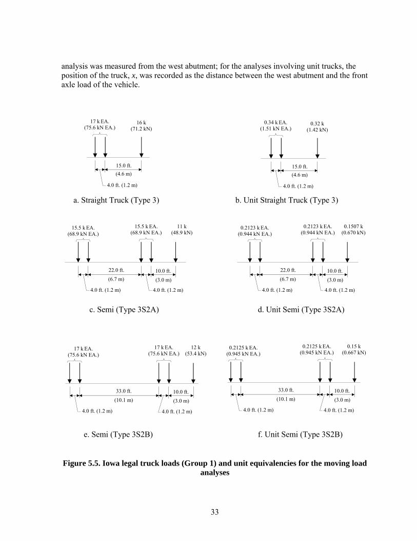
Figure 1.1. Typical Iowa FCB cross section....................................................................................2 Figure 1.2. Out-of-plane bending in the web gap due to relative girder displacement ...................2 Figure 1.3. Photographs of the US 30 bridge ..................................................................................5 Figure 1.4. Composition and layout of the US 30 bridge ................................................................6 Figure 2.1. Example of a univariate control chart [73]..................................................................14 Figure 2.2. Example of a regression control chart [73] .................................................................15 Figure 2.3. Superimposed univariate control charts with elliptical control regions [73] ..............15 Figure 3.1. The 210x20 mm SMS used for sensing in uniform strain fields.................................18 Figure 4.1. FOS layout of the FCB SHM system in the US 30 bridge..........................................20 Figure 4.2. Alignment of the FOSs in the cut-back regions of Cross Sections C and E ...............22 Figure 4.3. Overview of the US 30 FCB SHM system components .............................................23 Figure 5.1. Continuous 24-hr time history strain plots for selected FOSs ....................................27 Figure 5.2. Identification of B-SG-BF-H raw data file segments with constant baselines............28 Figure 5.3. Zeroed B-SG-BF-H data file segments .......................................................................30 Figure 5.4. Zeroed and filtered strain data for B-SG-BF-H (See Figure 5.3b)..............................31 Figure 5.5. Iowa legal truck loads (Group 1) and unit equivalencies for the moving load analyses33 Figure 5.6. Positioning and length of travel for the unit concentrated load and unit trucks in the

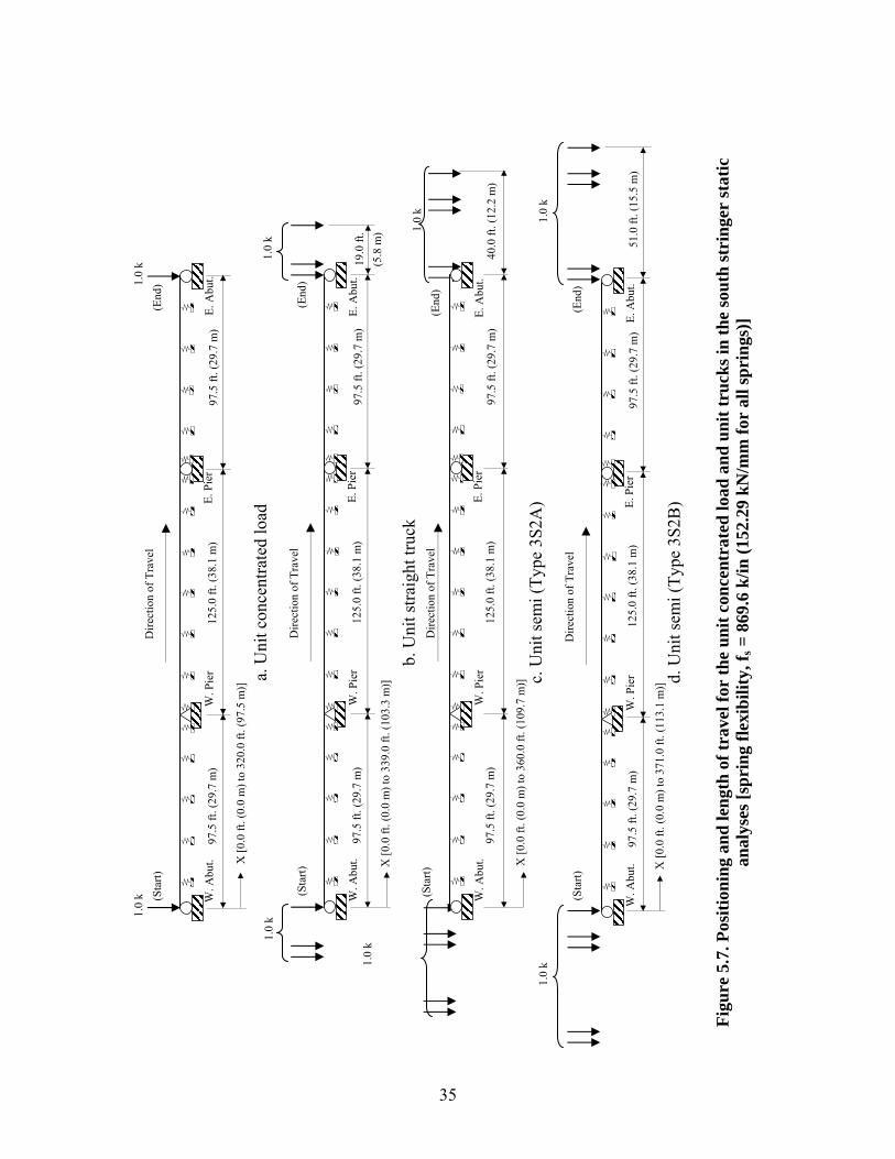
south girder static analyses ................................................................................................34 Figure 5.7. Positioning and length of travel for the unit concentrated load and unit trucks in the

south stringer static analyses [spring flexibility, fs = 869.6 k/in (152.29 kN/mm for all springs)] .............................................................................................................................35

Figure 5.8. A-SS-WB-V: experimental vehicular event and corresponding analytical reaction history ................................................................................................................................38

Figure 5.9. B-SS-BF-H: experimental vehicular event and corresponding analytical moment history ................................................................................................................................39

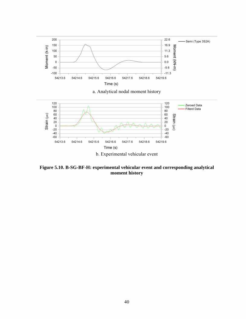
Figure 5.10. B-SG-BF-H: experimental vehicular event and corresponding analytical moment history ................................................................................................................................40

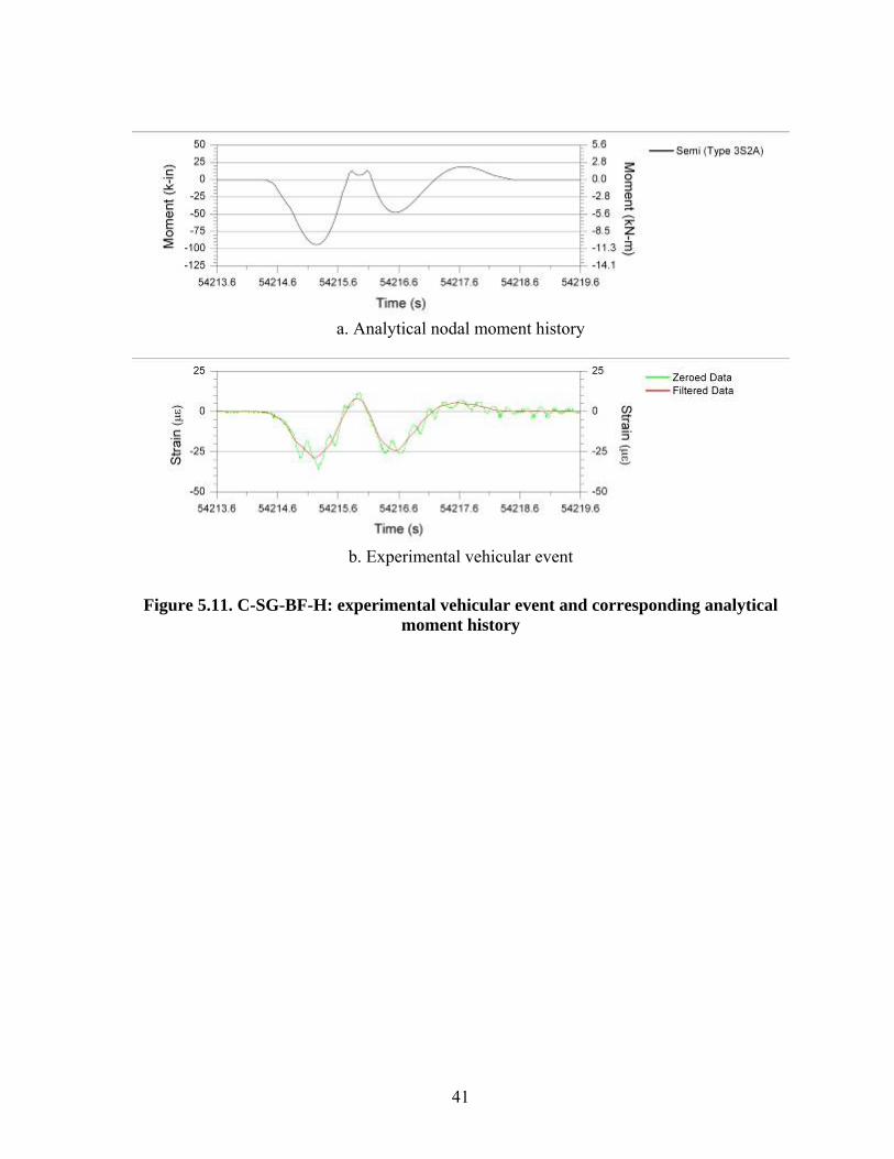
Figure 5.11. C-SG-BF-H: experimental vehicular event and corresponding analytical moment history ................................................................................................................................41

Figure 5.12. C-SS-WB-V: experimental vehicular event and corresponding analytical reaction history ................................................................................................................................42

Figure 5.13. D-SS-BF-H: experimental vehicular event and corresponding analytical moment history ................................................................................................................................43

Figure 5.14. D-SG-BF-H: experimental vehicular event and corresponding analytical moment history ................................................................................................................................44

Figure 5.15. E-SS-WB-V: experimental vehicular event and corresponding analytical reaction history ................................................................................................................................45

Figure 5.16. E-SG-BF-H: experimental vehicular event and corresponding analytical moment history ................................................................................................................................46

Figure 5.17. F-SS-BF-H: experimental vehicular event and corresponding analytical moment history ................................................................................................................................47

Figure 5.18. F-SG-BF-H: experimental vehicular event and corresponding analytical moment history ................................................................................................................................48

Figure 5.19. Identified extrema for a vehicular event in the B-SG-BF-H strain record (See Figure 5.4) .....................................................................................................................................49

viii

Figure 5.20. General flowchart for setup and monitoring modes of the FCB SHM system .........52 Figure 5.21. Out-of-plane bending measured by FOSs in the north cut-back region in the US 30

bridge .................................................................................................................................53 Figure 5.22. Out-of-plane bending measured by FOSs in the south cut-back region in the US 30

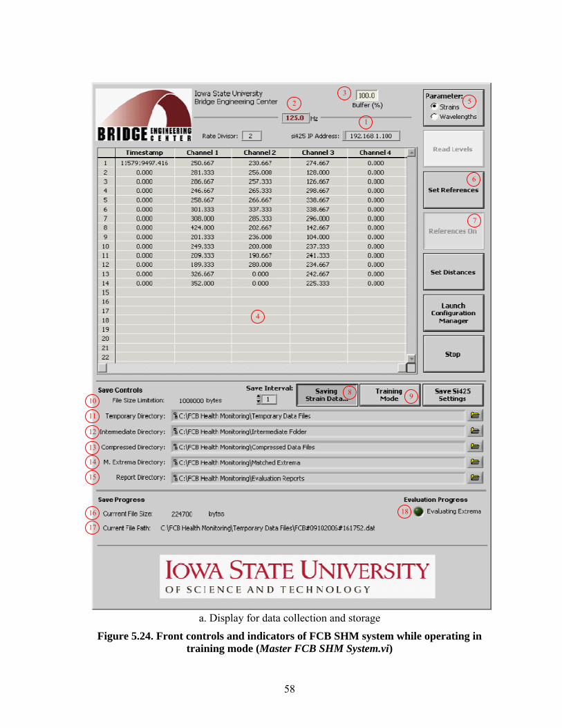
bridge .................................................................................................................................54 Figure 5.23. Overview of the steps included in the FCB SHM training process...........................56 Figure 5.24. Front controls and indicators of FCB SHM system while operating in training mode

(Master FCB SHM System.vi)............................................................................................58 Figure 5.25. Front panel controls and indicators for program generating PSD plots (1 - Perform

FCB FFT. PSD Analysis.vi)...............................................................................................65 Figure 5.26. B-SG-BF-H: power spectral density (PSD) plot with identified frequencies ...........68 Figure 5.27. Front panel controls and indicators for configuring the lowpass frequency filter (2 -

Configure FCB Filter.vi) ...................................................................................................69 Figure 5.28. Details of determining event extrema in a strain record with the subVI, Determine

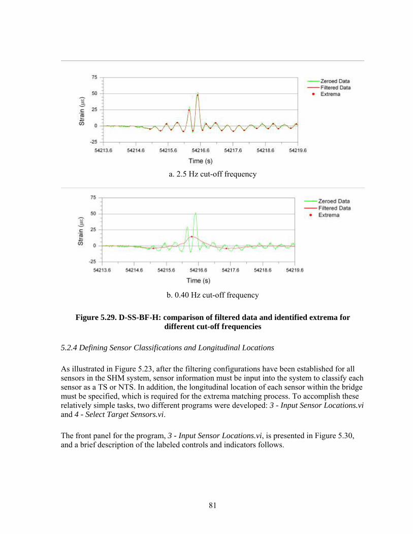
Extrema – One Sensor.vi ...................................................................................................75 Figure 5.29. D-SS-BF-H: comparison of filtered data and identified extrema for different cut-off

frequencies .........................................................................................................................81 Figure 5.30. Front panel controls for inputting sensor longitudinal locations (3 - Input Sensor

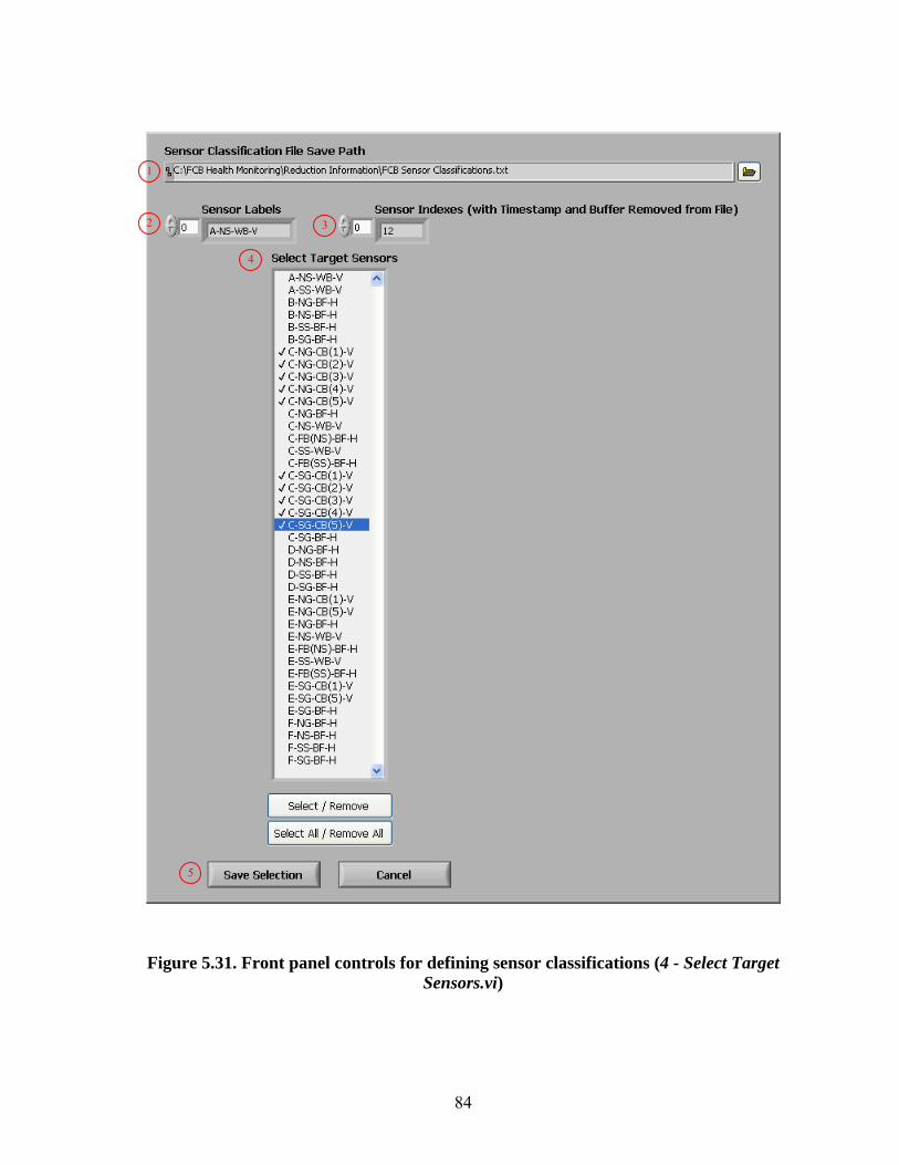
Locations.vi) ......................................................................................................................82 Figure 5.31. Front panel controls for defining sensor classifications (4 - Select Target Sensors.vi)84 Figure 5.32. Front panel controls for developing training files from raw data files (5 - Develop

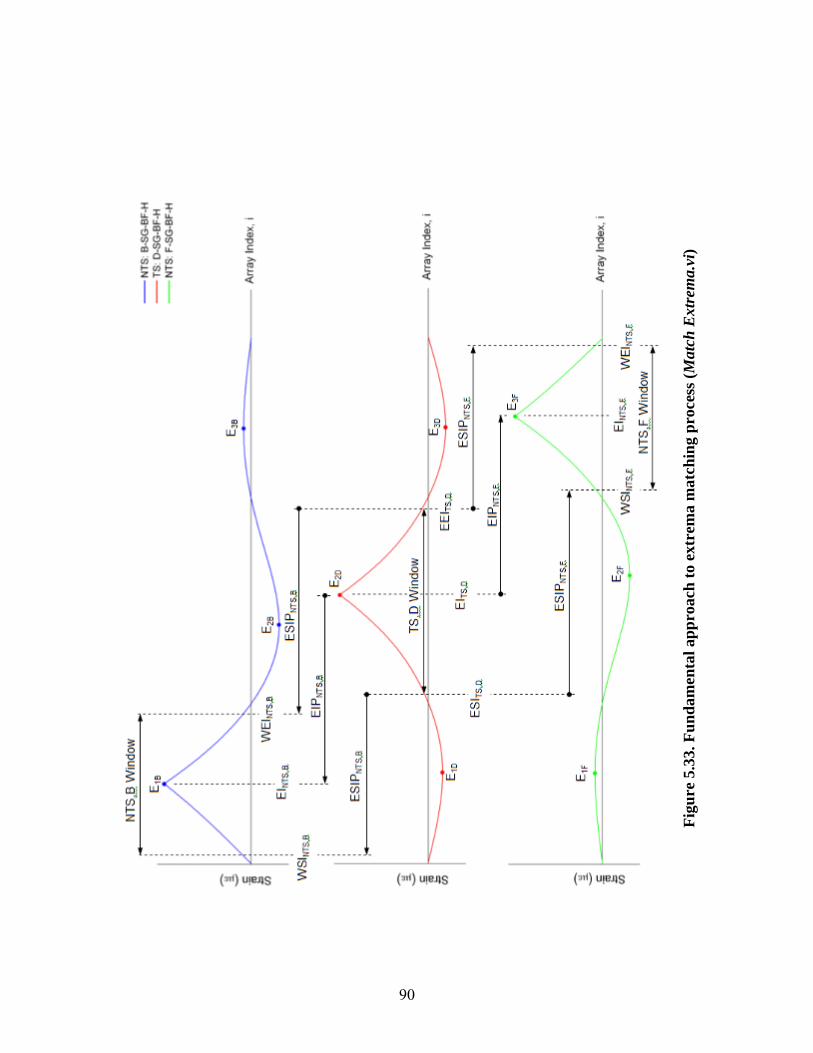
SHM Training Files.vi) ......................................................................................................88 Figure 5.33. Fundamental approach to extrema matching process (Match Extrema.vi) ...............90 Figure 5.34. Illustration of direct matches and indirect extrema matches (mismatches not

presented)...........................................................................................................................94 Figure 5.35. Example of extrema matching for 270 seconds of data from the US 30 SHM System95 Figure 5.36. Front panel controls and indicators for assembling the training files (6 - Assemble

SHM Training Files.vi) ......................................................................................................97 Figure 5.37. Front panel controls and indicators for reviewing assembled training data from one

directory (7 - View Results - Assembled SHM Training Files.vi)......................................99 Figure 5.38. Comparison of training data for various time periods (7 - View Results - Assembled

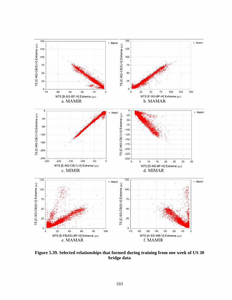
SHM Training Files.vi) ....................................................................................................102 Figure 5.39. Selected relationships that formed during training from one week of US 30 bridge

data...................................................................................................................................103 Figure 5.40. Comparison of changes in training relationships by altering the NTS cut-off

frequency..........................................................................................................................105 Figure 5.41. Front panel controls and indicators for establishing limit sets to define relationships

(8 - Define Limits.vi) ........................................................................................................107 Figure 5.42. Front panel controls and indicators for establishing limit sets to define relationships

(9 - View Results - Defined Limits.vi) ..............................................................................110 Figure 5.43. Selected limit sets that define relationships in the US 30 SHM system .................113 Figure 5.44. Overview of the phases in the FCB SHM monitoring process that are performed for

each data file ....................................................................................................................117 Figure 5.45. Front controls and indicators of FCB SHM system while operating in monitoring

mode (Master FCB SHM System.vi)................................................................................118 Figure 5.46. Identification of “pass” and “fail” relationship assessments for matched extrema.122 Figure 5.47. Comparison of daily evaluation reports for TSs in the US 30 SHM system...........125 Figure 5.48. Comparison of weekly evaluation reports for TSs in the US 30 SHM system.......130

ix

Figure 5.49. C-SG-CB(1)-V: Predicted changes in histogram patterns damage formation and growth ..............................................................................................................................134

LIST OF TABLES

Table 5.1. Sensor array indexes, longitudinal locations, and classifications.................................87 Table 5.2. Summary of defined relationships for TS-NTS combinations in the US 30 SHM

system ..............................................................................................................................115

xi

ACKNOWLEDGMENTS

The investigation presented in this report was conducted by the Bridge Engineering Center at Iowa State University. The research was sponsored by the Iowa Department of Transportation, Highway Division, and the Iowa Highway Research Board. Bruce Brakke of the Iowa Department of Transportation is acknowledged for his support of the project and for his technical input. Several other Office of Bridges and Structures personnel at the Iowa Department of Transportation provided input and support during the project and are also acknowledged, particularly Ahmad Abu-Hawash and Norm McDonald.

xiii

EXECUTIVE SUMMARY

This report is divided into two volumes. This volume (Volume I) summarizes a structural health monitoring (SHM) system that was developed for the Iowa DOT to remotely and continuously monitor fatigue critical bridges (FCB) to aid in the detection of crack formation. The developed FCB SHM system enables bridge owners to remotely monitor FCB for gradual or sudden damage formation. The SHM system utilizes fiber bragg grating (FBG) fiber optic sensors (FOSs) to measure strains at critical locations. The strain-based SHM system is trained with measured performance data to identify typical bridge response when subjected to ambient traffic loads, and that knowledge is used to evaluate newly collected data. At specified intervals, the SHM system autonomously generates evaluation reports that summarize the current behavior of the bridge. The evaluation reports are collected and distributed to the bridge owner for interpretation and decision making.

Volume II summarizes the development and demonstration of an autonomous, continuous SHM system that can be used to monitor typical girder bridges. The developed SHM system can be grouped into two main categories: an office component and a field component. The office component is a structural analysis software program that can be used to generate thresholds which are used for identifying isolated events. The field component includes hardware and field monitoring software which performs data processing and evaluation. The hardware system consists of sensors, data acquisition equipment, and a communication system backbone. The field monitoring software has been developed such that, once started, it will operate autonomously with minimal user interaction. In general, the SHM system features two key uses. First, the system can be integrated into an active bridge management system that tracks usage and structural changes. Second, the system helps owners to identify overload occurrence, damage and deterioration.

1

1. INTRODUCTION

For decades, structural health monitoring (SHM) has enabled bridge engineers to monitor the structural behavior of entire bridges or individual bridge components. Short-term SHM has dominated the field for most of its existence. However, technological advancements within the last decade have resulted in the evolution of long-term SHM, which has allowed for monitoring and evaluation of a bridge or bridge components continuously for years. As these systems have developed and proven their abilities, the degree to which bridge owners have invested, implemented, and utilized them has also increased.

1.1 Background

A fracture-critical bridge (FCB) is one that has at least one fracture-critical member (FCM) or member component; FCMs or member components are members whose failure would be expected to result in the collapse of the bridge [1]. There are more than 50 FCBs within the state of Iowa on the primary road system that were designed and constructed in the 1960s. A typical Iowa FCB has a two-girder cross section with stringers that are supported by floor beams, as illustrated in Figure 1.1; the welded plate girders are continuous over multiple spans, and the stringers are continuous over the floor beams. While the sizes of the structural members change to accommodate different span lengths for each bridge, the transverse spacing among the girders and stringers is constant for the FCBs in Iowa of this type.

When the FCBs were constructed, standard practice was to not weld stiffeners and connection plates to the girder tension flanges, due to concern that the strain concentrations from welds would cause fatigue cracks to form. This practice, unfortunately, merely moved the fatigue issue to other locations. Within a given cross section, the girders deflect different amounts, and the relative vertical displacement between the girders produces out-of-plane bending in the web gaps of connection plates that are not welded to the girder flanges (See Figure 1.2). This out-of-plane bending caused fatigue cracks to develop in the web gap areas above the floor beam connection plates in the negative moment regions (NMRs) in several of Iowa FCBs. The confinement of fatigue cracks to the NMRs is explainable when considering the boundary conditions that are imposed on the tension flange throughout the bridge. In the NMRs of a bridge, the concrete deck restrains the tension flange from rotating, whereas in the positive moment regions (PMRs), the tension flange is free to rotate. Because of the difference in rotational restraint, out-of-plane bending in the NMRs is usually larger than that in the PMRs; thus, the likelihood of fatigue crack formation increases. The magnitude of the out-of-plane bending is heavily influenced by the girder spacing and bridge skew. For example, the relative displacement between girders at a cross section will be larger for skewed bridges, which produces larger out-of-plane bending in the web gaps [2].

With concern of the fatigue cracks propagating vertically through the girders and causing structural failure, retrofit procedures were developed and implemented in the FCBs. Each retrofit involved cutting back the floor beam connection plates and any accompanying stiffeners in the NMR to reduce out-of-plane bending stress levels.

2

Figure 1.1. Typical Iowa FCB cross section

Figure 1.2. Out-of-plane bending in the web gap due to relative girder displacement

During the retrofit of the US 151 bridge, a 67.5-in. (1.7-m)- long crack spontaneously propagated vertically through the girder web. The US 151 crack formation is an example that illustrates the severe dangers that fatigue cracks impose on FCBs, and as a result of this threat, FCBs are manually inspected for fatigue cracks during their biennial inspections. However, the Iowa DOT expressed interest in a SHM system with the ability to monitor the FCBs continuously between inspections. With advanced identification of crack development, necessary bridge repair can be accomplished before cracks have reached a critical state that causes bridge failure.

1.2 Scope and Objective of Research

The SHM system developed in this study has been developed for the Iowa DOT bridge engineers to remotely and continuously monitor a FCB in order to aid detection of crack formation by identifying gradual changes in bridge structural behavior. The specifications for the system were identified as follows:

Relative Girder Displacement

Out-of-Plane Bending in Web Gap

Displaced Girder

3

• Monitoring must be continuous and capable of identifying changes in bridge structural behavior (elastic or inelastic) from a preexisting state, which may be indicative of crack development and/or propagation.

• Data collection, reduction, evaluation, and storage must be autonomous. • Summaries of reduced data and evaluations must be presented in a clear,

understandable format to bridge engineers; the presentation of the data must be in a report that is autonomously generated and electronically delivered.

• DOT work forces with proper training must be capable of installing the system.

Previous experience with long-term SHM at the ISU BEC resulted in the accumulation of massive amounts of data, but it was determined that only a small percentage of the data were useful for assessing the condition of the structure [3]. As a result, in addition to the previously defined objectives, this study also included significant efforts to (1) develop data reduction procedures that identify and extract the information in data files that is useful for evaluating the condition of the bridge, and (2) develop evaluation methods that effectively utilize the extracted data to correctly report the structural condition of the bridge.

1.3 Proposed SHM Solution

The proposed SHM solution is a monitoring system that utilizes strains measured at various locations that result from ambient traffic crossing the bridge. Strain has been selected as the damage detection parameter in this study because it is a highly dependent indicator of damage, and in addition, it is usually the parameter that is best understood by bridge engineers. In this approach, sensors are installed in regions of the bridge that are expected to experience damage, such as the cutback region of the retrofit, and also in regions of the bridge that are not expected to experience damage. Fiber optic sensors (FOSs) have been chosen as the strain sensors based on previous success with long-term strain monitoring and distinct advantages that are discussed subsequently.

The recorded strains resulting from ambient traffic for a given period of time are used to develop relationships between sensors in the damage prone regions of the bridge and those that are not in damage prone regions of the bridge; each relationship is formed and defined with upper and lower limits similar to the methods used with control chart analyses. By developing the relationships with recorded strain data, the system has been trained to recognize typical performance for the existing condition of the bridge.

After the relationships have been established, they are used to evaluate every traffic event measured by the system. The assessment from each relationship is “Pass” or “Fail”, and at the end of a specified evaluation period, the assessments are summarized in histograms. Structural changes in the bridge, such as the formation of cracks, are expected to be evident through changes in histogram distributions for successive evaluation periods.

4

1.4 SHM System Demonstration Bridge

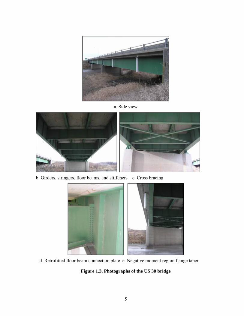
The Iowa FCB that was selected as the demonstration bridge for the showcased project is the US Highway 30 (US 30) bridge crossing the Skunk River near Ames, IA (See Figure 1.3). The demonstration bridge has a 30-ft. (9.1-m)- wide roadway that supports two east-bound traffic lanes; the posted speed limit is 65 miles per hour (mph) [105 kilometers per hour (kph)]. The composition and layout of the bridge is presented in Figure 1.4. As illustrated, the bridge is a three span structure consisting of 97.5-ft. (29.7-m)- long side spans and a 125-ft. (38.1m)- long middle span. Review of Figures 4a-b reveals that the floor beam connection plates in the NMR have been cut back during the retrofit procedure, whereas those in the PMR have not been cut back. To date, no fatigue cracks have developed in the cut-back regions of the girders above the floor beam connection plates in the US 30 bridge.

1.5 Report Content

The contents of this report discuss all aspects of the development of the proposed SHM system. The information in Chapter 2 provides a brief overview of the current international state of SHM in bridge structures. Presented in Chapter 3 are the procedures that were used to select the technology for this research, and in addition, the laboratory validation testing that was performed to ensure that the technology was suitable for use in the SHM system. Chapter 4 illustrates the hardware layout at the US 30 bridge and presents the in-service validation testing that was performed. In Chapter 5, the SHM system software is discussed; the details of the operations that are performed by the system are described, and examples of collected and analyzed data are provided. Finally, Chapter 6 summarizes the conclusions that were determined from the research, and Chapter 7 provides recommended future research that is required to further expand the SHM system that was developed.

5

a. Side view

b. Girders, stringers, floor beams, and stiffeners c. Cross bracing

d. Retrofitted floor beam connection plate e. Negative moment region flange taper

Figure 1.3. Photographs of the US 30 bridge

6

a. Cross section in positive moment regions b. Cross section in negative moment regions

c. Layout of structural steel, identification of positive and negative moment regions, and locations of cut-back retrofits

Figure 1.4. Composition and layout of the US 30 bridge

7

2. LITERATURE REVIEW

The material presented in this chapter provides a general overview of the state of bridge SHM. However, for the topics pertaining to the development of the FCB SHM system discussed in Section 1.3, specific attention and detail is provided.

2.1 Background to Field Inspection of Bridges

The need for a structured method of recording and tracking the condition of bridges in the United States became evident in 1967 when the Silver Bridge between Point Pleasant, West Virginia, and Gallipolis, Ohio, collapsed during rush hour traffic, resulting in the deaths of 46 civilians. In response, the National Bridge Inspection Standards (NBIS) were implemented in the 1970s to guide the inspection and inventory of bridges on public roads. In general, bridges are inspected every two years with exceptions given to bridges with special conditions that warrant shorter or longer inspection cycles [4].

The evaluations of each bridge in the NBI currently rely heavily on visual inspections. For many years visual inspection was the only alternative to evaluating a bridge, and the method has advantages in terms of cost and ease of application [5]. However, its limitations have been shown to sometimes result in inconsistent and erroneous bridge evaluations [7]. The limitations of visual inspection are the result of many factors, and two of the major ones are that (1) they are subject to the opinions and variability in experience and training among the inspectors, and (2) they are limited to structural condition that can only be perceived by the human eye, and thus, if signs of damage are not visually evident, such as subsurface cracks, then they may be overlooked and not included in the evaluation.

Bridge owners spend a large portion of their budget inspecting and maintaining bridges within their inventory. Unfortunately, FCBs have been proven to consume a large fraction of that budget even when they represent a small fraction of the bridge inventory. In a National Cooperative Highway Research Program (NCHRP) synthesis study [6], bridge owners reported that FCBs cost two to five times the amount to inspect than redundant bridges.

2.2 Crack Detection with Advanced Methods

2.2.1 Crack Detection with Conventional Technology

As previously mentioned, past research involving crack detection has involved vibration-based sensing and strain-based sensing, which involves the use of accelerometers and strain gages, respectively. A basic understanding or estimation of the event being measured is critical to the accuracy of the measurement in either case. With accelerometers, the amplitude and frequency content of the event are required for proper accelerometer selection. With conventional strain gages, two common types of sensors are available and selected based on the type (static or dynamic) of event being measured. Electrical resistance strain gages, also

8

known as foil gages, are capable of measuring dynamic events, but they have low zero-stability which ultimately results in signal drift.. Vibrating wire strain gages have high zero-stability, but they can only be used for quasi-static strain measurement [20]. Applications of accelerometers, strain gages, and piezoelectric sensors for crack detection are discussed in the following paragraphs.

Yoo and Kim [21] suggested that damage detection is a localized phenomenon, and as a result, the sensor being utilized must also measure a localized response. The project presented analytical work to illustrate the use of strain measurements to determine strain mode shapes of in a plate before and after crack formation. Results concluded that a cross grid (strain gages directly above and to the sides of a crack) of five sensors was sufficient to characterize the strain modes for crack detection. In addition, this method was analytically proven to identify the existence of a crack, but not the size crack. The results of this research were not experimentally tested, however.

Patil and Maiti [22] presented another analytical study that involved detection of multiple cracks in slender Euler-Bernoulli beams. This approach is one of few that is capable of identifying more than one crack at a time. The method was based on transverse vibration (natural frequencies) in the beam at one point. The beam was divided into a number of segments, and each segment was associated with a damage parameter. Through knowledge of changes in natural frequencies of the beam, damage parameters such as crack size and location were determined. Several successful numerical examples were presented, but the method was not proven experimentally.

2.2.2 Crack Detection with Fiber Optic Technology

As technology has continued to improve, so has the market for sensors. Within the last decade, fiber optic technology has evolved and been researched to demonstrate its potential for crack detection. In the proceeding paragraphs, a background for fiber optic sensing is presented along with selected research projects that utilize the technology for crack detection.

Fiber optic sensors measure some type of change in guided light, and two general categories of FOSs exist based on where the change in guided light is measured: intrinsic (inside the fiber) and extrinsic (outside the fiber). The four primary changes in guided light that can be measured are as follows: phase, polarization state, intensity, and wavelength. Thus, four refined categories of FOSs are as follows, respectively: (1) interferometric sensors, (2) polarimetric sensors, (3) intensity modulated sensors, and (4) spectrometric sensors. Intensity modulated sensors and spectrometric sensors are the most commonly used strain sensors [29].

Hale [32] presented some of the earliest attempts to use fiber optic technology for crack detection in a specimen. In the research, a prepackaged crack-detection sensor was developed. The sensor was designed to be bonded to a structure in the crack-prone region. If

9

a crack formed in the substrate material below the sensor, the optical fiber was damaged or broken; thus, light being transmitted through the fiber was attenuated, and the measured attenuation change was indicative of structural cracking. Each sensor was designed with three parallel optical fibers, an attempt to monitor crack propagation through sequential damage in the fibers. Infrared light sources and detectors were displayed in the research, but it was also suggested that OTDRs could be used. Simple laboratory tests on tensile coupon proved that the sensor is capable of detecting cracks as small as 5–30µm.

Leung et al. [33, 34] illustrated a fully distributed fiber optic network with OTDR to determine crack formation and/or propagation. The method consisted of installing a single mode fiber (SMF) in a ‘zigzag’ pattern throughout a region where cracks were expected to develop in a concrete structure. Before the formation of cracks, the OTDR was used to establish a baseline of signal intensity versus fiber length. If a crack formed in the structure at an angle other than 90° to the fiber, a sharp bend formed in the fiber and caused a significant drop in the power signal on the OTDR record. The location of the crack was known based on the OTDR record, and the magnitude of the drop was related to the size of the crack. Olson et al. [35] demonstrated theoretically and experimentally that using this approach with multimode fiber (MMF) increased the dynamic range of the measurement, which is the total loss that can be monitored. Thus, more cracks were able to be monitored by the network with MMF.

Yang et al. [36] showcased a procedure to use integral strains (total change in length of the fiber) to detect the presence of cracks in a specimen. Fibers were bonded to a surface expected to crack, and when the crack formed, the change in length of the fibers (deformation of the specimen) were determined by measuring phase shift’s of the system and were used in an algorithm to determine the crack size and location. Numerical models were presented to support the research, but experimental procedures were not performed.

2.3 Structural Health Monitoring for Damage Detection in Bridges

Structural health monitoring is a broad term used to describe monitoring that produces an overall depiction of the structure’s condition. Thus, SHM should not be considered as only damage detection; damage detection is just one aspect of SHM. Within the last decade, research pertaining to continuous field monitoring of bridges has increased dramatically. A few of the major factors contributing to the increase in SHM research include the following [41]:

• The current state of the aging bridge infrastructure and economics associated with rehabilitation and repair versus new construction.

• Technological advancements such as increases in computing memory and speed, as well as advancements in sensors.

• Recent failures receiving media coverage, which in turn creates public concern, political pressure, and increased funding for research.

10

In addition to the complexities of detecting damage in controlled laboratory experiments, SHM that includes damage detection for in-service bridges introduces more challenges:

• The system components and functionality must be capable of withstanding and compensating for environmental conditions such as extreme temperatures, moisture, wind, etc.

• The structure being monitored is larger and more complex. • The magnitude and frequency of external loads on the structure cannot be

controlled for most practical in-service monitoring approaches. • Power for electrical equipment may not be available due to the remote location of

some bridges, and solar power equipment may not be suitable to supply sufficient electricity for some SHM systems.

• Wireless communication is usually the only practical method to communicate with SHM components at the bridge site, which is slower and less reliable than wired communication that is typically available in laboratories.

2.3.1 Background to Structural Health Monitoring Procedures

The complexity and capability of SHM systems are different, and thus, the information pertaining to structural condition and/or damage that is presented to the bridge engineer varies for each system. Research by Rytter [42] defines four levels of damage detection:

• Level 1: Determination that damage is present in the structure • Level 2: Determination of the geometric location of the damage • Level 3: Quantification of the severity of the damage • Level 4: Prediction of the remaining service life of the structure

Level 1 is a forward problem that identifies a change in a parameter and relates it to the presence of damage. Levels 2 and 3 are inverse procedures that use the change in the parameter to back-calculate the extent and location of the damage that caused the parameter change. Some type of modeling is usually required to reach Level 3 damage detection.

2.3.2 Structural Health Monitoring of Bridges with Conventional Technology

Most SHM bridge projects have utilized conventional technology to accomplish their sensing needs. These projects include SHM on FCBs similar to the US 30 bridge (Figure 1.6) as well as many redundant styles of bridges. Selected research projects pertaining to each category are presented in the subsequent sections.

2.3.2.1 Monitoring of Fracture-Critical Bridges

In 1993, the I-40 bridges over the Rio Grande in Albuquerque, NM, were scheduled to be demolished, creating an opportunity to investigate the post-damage performance of a full

11

scale bridge. The I-40 bridges were classified as fracture-critical since they were two-girder designs very similar to the US 151 and US 30 bridges. There were two primary differences between the designs of the I-40 bridges and the designs of the US 151 and US 30 bridges: (1) the I-40 bridges had three stringers positioned between the two exterior plate girders, while the US 151 and US 30 bridges have two stringers, and (2) the I-40 bridges had cross bracing between each set of floor beams, but the US 151 and US 30 bridges only have diagonal bracing between floor beams near the piers.

The research approach consisted of first testing the bridge in the pristine condition, and then the bridge was retested after damage was inflicted to the middle span of the three-span segment of the bridge. The damage consisted of four sequential cuts to the web and bottom flange of an exterior girder at midspan of the middle span; the final damage case resulted in a cut that completely severed the bottom flange and extended upward through approximately 60% of the web. Two different parameters, vibrations [44, 45, 46] and strains [47], were utilized to scrutinize three different SHM approaches.

Farrar and Jauregu [44] used two sets of accelerometers to measure the I-40 bridge accelerations; one coarse set of accelerometers measured the global response of the bridge over the three spans, and a refined set that was confined to the damaged area of the bridge. A hydraulic shaker was used to subject the structure to a random vibration signal over the range of 2 to 12 Hz. Many analyses were performed to investigate the changes in bridge properties due to damage and included changes in resonant frequencies, mode shapes, mode shape curvature, load surface curvature, flexibility, and stiffness. Results from the study indicated that resonant frequencies and mode shapes were poor indicators of damage and that all other methods did not clearly identify damage until the most severe damage case when the entire bottom flange and 60% of the web were cut. The researchers also conducted a follow-up study [45] that investigated the accuracy the damage identification methods when applied to numerical models. Conclusions from the numerical study were approximately the same as those of the experimental study.

Woodward et al. [46] describe the analysis that was conducted on the I-40 bridge that utilized the resonant ultrasound spectroscopy (RUS) method, which relies on changes in the resonant frequencies of the structure as indicators of damage. While the structure was vibrated with the driving force from low to high frequency, a narrow band measurement was swept over the same frequency range. Since noise is significantly reduced with this method, slight changes in frequencies and mode shapes were detectable. Results of the study indicated that only the most severe case of damage was identifiable.

2.3.2.2 Monitoring of Redundant Structures

Most projects involving SHM are demonstrated on redundant structures. A review of literature for these projects reveals a wide variety of sensors that have been utilized among the most successful projects: accelerometers, strain gages, load cells, displacement transducers, level sensors, anemometers, temperature sensors, weigh-in-motion sensors, etc. Although the selected projects presented in this section attempt to illustrate the broad use of

12

these sensors, vibration-based monitoring has been investigated far more than any other method.

Kesavan et al. [49] analytically illustrated the use of static strain distributions with an ANN to detection delaminations in a glass fiber reinforced polymer (GFRP) retrofit. Strain distributions obtained from FEA for various damage scenarios were used to train an ANN. Results of the study concluded that as distances between strain gages on the FEA decreased (more sensors in the area of damage), the percentage of error for the ANN decreased.

Wong et al. [50] presented the Wind And Structural Health Monitoring System (WASHMS) installed on the Tsing Ma Bridge, Kap Shui Mun Bridge, and Ting Kau Bridge. The systems installed on these bridges are some of the largest and most diverse to date. Approximately 774 sensors have been installed on these suspension and cable-stayed bridges and include the following: accelerometers, strain gages, displacement transducers, level sensors, anemometers, temperature sensors, and weigh-in-motion sensors. Data are interpreted in the amplitude, time, and frequency domains for analysis and interpretation. Several examples of data collected were presented. Li et al. [51] demonstrated the use of strain gage measurements in a fatigue damage model to estimate the remaining fatigue life of the Tsing Ma Bridge. In addition, Ni et al. [52] illustrated the use of probabilistic neural networks (PNNs) for damage identification and location in the Ting Kau Bridge.

Caicedo and Dyke [53] presented the use of accelerometers to measure changes in dynamic characteristics of a cable-stayed bridge to detect damage. The method was developed utilizing information from FEA, and then it was compared to results from experimental testing on a scaled laboratory model in both the undamaged and damaged state. Results of the testing indicated that damage was detectable in the structure by comparing natural frequencies for the undamaged and damaged bridge.

2.3.3 Structural Health Monitoring of Bridges with Fiber Optic Technology

As previously mentioned, FOSs are available as accelerometers, strain gages, tilt meters, displacement transducers, temperature sensors, load cells, etc., and as a result, have been incorporated into many SHM systems. Further description of a variety of monitoring approaches are described in the following paragraphs.

Some of the earliest uses of fiber optic sensors are illustrated by Tennyson et al. [59] and Maalej et al. [60]. Six bridges in Canada were instrumented with FBGs for a variety of monitoring applications. The Beddington Trail, Taylor, and Joffre Bridges were primarily instrumented with FOSs to evaluate the immediate and long-term performance of GFRP and carbon fiber reinforced polymer (CFRP) as prestressing tendons, as well as flexural and shear reinforcement. The Crowchild Trail Bridge and Salmon River Bridge were the first bridges to be constructed with steel-free decks. Transverse steel straps across the tops of the girders provide transverse confinement to the deck. Strain gages consisting of foil resistance gages, FBGs, and Fabry-Perot sensors were installed on the girders, transverse steel straps, and in

13

the deck to monitor the performance of the new designs. Finally, the Confederation Bridge, which is the longest bridge over iced-ocean water, was instrumented with FBGs to monitor its loadings and structural performance to ensure that it is maintaining adequate strength in the harsh environment. For nearly every bridge, temperature sensors were installed to help temperature-compensate the FOS.

Doornink et al. [61], Graver et al. [62], as well as Phares and LaViolette [63] describe the use of FBG sensors to monitor the performance of new materials. A high-performance steel (HPS) bridge was continuously monitored with 40 FBG sensors to determine its structural response to ambient traffic traversing the bridge. In addition, the performance of a prestressed, UHPC beam was laboratory tested to verify its shear and flexural properties to aid the design of the first UHPC bridge in the USA.

Doornink et al. [65] as well as Phares and LaViolette [62] demonstrate the use of FBGs to help guard a historic covered bridge in Madison County, IA from arson. The FBGs installed on the bridge measure the temperature of the wood to detect fire. Flame detectors and infrared cameras were also installed in conjunction with the FBGs. When the components of the SHM system agree to the presence of fire, authorities are autonomously alerted.

Yong et al. [70] presented a fiber optic SHM system for the monitoring of the Dafosi Bridge, the largest cable-stayed bridge across the Yangtze River in western China. The system monitors fiber optic strain sensors, displacement sensors, temperature sensors, and dynamic measurements to evaluate the structural condition of the bridge. Evaluation of data includes on-site preprocessing before it is sent to a host computer at a management center for further evaluation.

2.3.4 Feature Discrimination in Structural Health Monitoring for Damage Detection

Feature (or parameter) discrimination has received the least amount of attention in scientific literature. Feature discrimination often incorporates some kind of statistical methods to operate on the extracted features or parameters to determine the extent of the damage. As previously mentioned, statistical-based feature discrimination algorithms utilize either supervised or unsupervised learning. Examples of supervised learning in literature include response surface analysis, Fisher’s Discriminant, neural networks, genetic algorithms, and support vector machines; examples of unsupervised learning include control chart analysis, outlier detection, neural networks, and hypothesis testing. Neural networks are perhaps the most popular of all algorithms, while control chart analyses are less commonly used [43].

Control chart analyses have been heavily utilized for process controls of chemical plants, manufacturing facilities, and nuclear power plants [43], but have been utilized far less in SHM of bridges. Control charts are one of the primary techniques of statistical process control (SPC). The concept recognizes that every process has variation. Some of the variation in the process is unavoidable, always present, and inherent to the process. This type of variation is referred to as unassignable cause, common cause, or chance cause. Other types

14

of variation not always present, can be avoided with proper investigation, and are not normal to the process; this type of variation is termed assignable cause or special cause [72, 73].

To develop a control chart, information pertaining to a process characteristic, or parameter, is monitored and plotted versus time or sample number. A centerline (average expected values), upper control limit (UCL), and lower control limit (LCL) is developed to identify typical process behavior, which includes common cause variations. Each limit is typically established three standard deviations from the centerline, and thus, will statistically include 99.7% of all data points for the parameter if it is a normalized set. The area bounded by the limits is defined as the control region, which is applied to future parameter values for identifying new data (outliers) that are inconsistent with past data [72, 73].

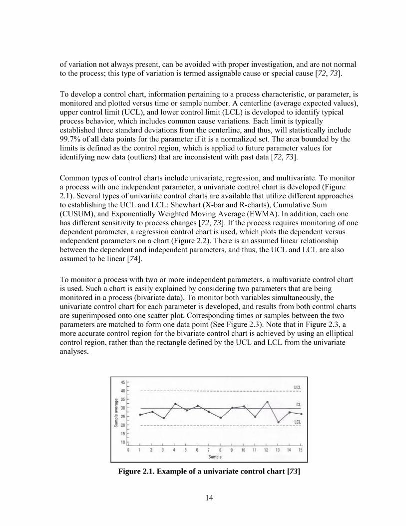
Common types of control charts include univariate, regression, and multivariate. To monitor a process with one independent parameter, a univariate control chart is developed (Figure 2.1). Several types of univariate control charts are available that utilize different approaches to establishing the UCL and LCL: Shewhart (X-bar and R-charts), Cumulative Sum (CUSUM), and Exponentially Weighted Moving Average (EWMA). In addition, each one has different sensitivity to process changes [72, 73]. If the process requires monitoring of one dependent parameter, a regression control chart is used, which plots the dependent versus independent parameters on a chart (Figure 2.2). There is an assumed linear relationship between the dependent and independent parameters, and thus, the UCL and LCL are also assumed to be linear [74].

To monitor a process with two or more independent parameters, a multivariate control chart is used. Such a chart is easily explained by considering two parameters that are being monitored in a process (bivariate data). To monitor both variables simultaneously, the univariate control chart for each parameter is developed, and results from both control charts are superimposed onto one scatter plot. Corresponding times or samples between the two parameters are matched to form one data point (See Figure 2.3). Note that in Figure 2.3, a more accurate control region for the bivariate control chart is achieved by using an elliptical control region, rather than the rectangle defined by the UCL and LCL from the univariate analyses.

Figure 2.1. Example of a univariate control chart [73]

15

Figure 2.2. Example of a regression control chart [73]

Figure 2.3. Superimposed univariate control charts with elliptical control regions [73]

The ellipses and regions identified in Figure 2.3 represent the following [73]:

• Ellipse A: Control region for parameters that are not correlated • Ellipse B: Control region for parameters that are negatively correlated • Ellipse C: Control region for parameters that are positively correlated • Region E and Region F: Additional areas to the control region that results from

using an elliptical control region rather than rectangular region • Region G: Area removed from the control region due to an elliptical control

16

region rather than a rectangular control region

3. SHM TECHNOLOGY EXAMINATION AND SELECTION

During the design of a SHM system, the measured parameters for assessing the condition of the structure must first be determined, and then the hardware components can be selected to perform the measurement and to function with other system components. The proceeding sections of this chapter discuss this process for the developed system

3.1 Parameter Selection for Discrimination and Damage Detection

As previously mentioned, strain was selected as the parameter for discrimination and damage detection. Selection of this parameter was based on (1) ease of its measurement and collection while ambient traffic crosses the bridge and (2) flexibility in the formats that can be used to present the results. With these considerations, the SHM system was designed to measure and analyze a reliable parameter while maintaining usefulness and attractiveness.

As mentioned in Chapter 2, two primary parameters have been researched and investigated for use in SHM systems for damage detection: vibrations and strains. Vibrations have been utilized more frequently than strains in previous research. One attractive feature of vibration-based monitoring that has contributed to its popularity is that the dynamic properties of a bridge are generally not affected by the magnitude of the events (weight of traffic). This eliminates an unknown involved in any monitoring that utilizes ambient traffic loads. However, most literature discussing results from these SHM systems agrees that there are notable limitations of using vibration-based measurements and dynamic properties for bridge damage detection:

An unfavorable characteristic of FBG sensors, which were selected for the developed system, as previously mentioned, is that they are sensitive to temperature variations. Thus, for any event occurring simultaneously with temperature fluctuations, FBG sensors measure the thermal and mechanical strain of the host material as well as an apparent strain resulting from temperature effects on the sensor itself. Compensation for this issue was avoided in the FCB SHM system by utilizing only mechanical strain measurements resulting from vehicles traversing the bridge. These events occur too quickly for temperature variation to simultaneously occur.

The dependency of strain on magnitude of loading was previously considered to be favorable because it creates a large population of events for evaluation, but it also creates difficulties since the weights of the ambient traffic events are not known. This challenge, however, was overcome in the FCB SHM system by using relative relationships among the sensors on the bridge, rather than an analysis that utilizes independent measurements from each sensor. The SHM data reduction techniques will be discussed in further detail in Chapter 5.

17

3.2 Conceptual Equipment Specifications

Equipment specifications must be considered for both the data acquisition equipment and strain sensors together to ensure proper system operation. For fiber optic sensing, the interrogator performs the data acquisition and must be capable of sampling at adequate rates for the event being recorded. As discussed in Section 2.5.2, a DAR of 10–20 times the maximum frequency in the strain record is sufficient to avoid filter aliasing effects and to accurately determine peak strain values within the record. Strain records for measured bridge responses typically include both quasi-static and dynamic frequencies from traffic events; fundamental frequencies for highway bridges are usually within 2–5 Hz [77], and quasi-static frequencies are often slower than the dynamic frequencies. Thus, to capture quasi-static events and the fundamental dynamic responses of most typical highway bridges, a DAR of 50–100 Hz is adequate. The Micron Optics si425-500 interrogator has sampling capabilities as high as 250 Hz, and thus, was determined to be adequate for use in the FCB SHM system.

Sensor specifications were investigated to ensure accurate measurements. As presented in Section 2.2.2, the conversion of FBG reflected spectrums to strains requires an understanding of the strain field being imposed on the FBG. Standard FBGs with 10mm lengths are sufficient in relatively uniform strain fields, but shorter FBGs are required in non-uniform strain fields. As a result, locations for strain measurements in the FCBs were identified, and the corresponding structural responses were considered to determine sensors specifications. Keeping in mind that large and repeatable strain measurements are most the most dependable strains within a record, and thus desirable for use in SHM, five different sensor orientations and locations were identified:

• Vertical orientation: cut-back regions of the retrofits and stringer webs above floor beams

• Horizontal orientation: bottom flanges of girders, stringers, and floor beams

Horizontal strains on bottom flanges of structural members develop from global bridge responses, and thus, those regions were assumed to have uniform strain fields that were measurable with FBGs having 10mm lengths. However, vertical strains in the retrofit cut-back regions and stringer webs above floor beams measure local bridge responses. A uniform strain field was assumed for the local vertical response of the stringer webs, and thus, 10mm FBGs were again considered to be suitable. However, the reverse curvature condition in the retrofit cut-back regions was considered to create a non-uniform strain field that required shorter FBG lengths. Thus, 5mm FBGs were selected to measure strains in the retrofit cut-back regions.

Previous bridge research involving FBG sensors at ISU [3] utilized surface-mountable sensors (SMSs) that were manufactured by Avensys, Inc. A photograph of a 210x20 mm SMS is given in Figure 3.1. Each SMS consists of a 10mm FBG with polyimide recoating that was embedded within a 210x20x1 mm (length x width x thickness) CFRP packaging. The CFRP packaging protected the sensor and made it more robust for installation purposes, and at the same time, increased its bonding surface area. The fiber pigtails exiting from each

18

side of the packaging (entry fiber and exit fiber) consist of SMF simplex cable (3 mm jacketing) and FC/APC mechanical connectors. To bond the 210x20 mm SMS to the bridge, Loctite 392 adhesive with Loctite 7387 activator were used. The field installation and performance of this sensor was proven in the previous research, and as a result, was selected as the sensor for use in all strain fields identified as suitable for measurement with a 10 mm FBG.

Figure 3.1. The 210x20 mm SMS used for sensing in uniform strain fields

For sensing in the retrofit cut-back regions, the size of the FBG and packaging of the 210x20 mm SMS was determined to be unsuitable. It was desired to use 5 mm FBGs to measure strains every 2 in. (55 mm) along the height of two cut-back regions, as well as at the top and bottom of other cut-back regions. To achieve this sensing, two different types of SMSs were envisioned and designed: (1) a single 5 mm FBG encased in a small form factor (SFF) CFRP packaging, and (2) an array of 5 mm FBGs entirely encased in a single CFRP packaging. Once again, each FBG utilized polyimide recoating, but the SMF pigtails exiting from each side of the packaging had 900 µm furcation tube for protection and did not have mechanical connectors.

Laboratory validation testing was performed to ensure that the interrogator, sensors, adhesives, and accessory equipment were capable of achieving the desired measurements and to reduce the likelihood of hardware deficiencies and malfunctions after field installation. This testing which is not summarized herein in the interest of brevity, was deemed to successfully validate the operation of all selected components.

19

4. FCB SHM SYSTEM HARDWARE

The hardware components that were implemented in the FCB SHM system include a FOS network, data collection and management equipment, and wireless communication equipment. The proceeding sections present an overview of the system bridge components as well as field validation testing procedures that were performed.

4.1 SHM System Components

Section 3.4 briefly mentioned the hardware components that were selected for use in the FCB SHM system based on their performance during the laboratory validation testing. The following sections provide information regarding the configurations and abilities of the components to function together to achieve the strain-based monitoring process.

4.1.1 Fiber Optic Sensor (FOS) Network

Forty FBG-based FOSs (SMSs and SMAs) were strategically distributed in six cross sections of the US 30 bridge. Figure 4.1a identifies the six cross sections, and Figures 4.1b–g illustrate the locations and orientations of the sensors within each section. Each FOS has been assigned a label with the following format:

Section – Member – Part – Orientation where, BF = Bottom flange NS = North stringer CB = Cut-back region SG = South girder FB = Floor beam SS = South stringer H = Horizontal V = Vertical NG = North girder WB = Web The instrumentation layout was specifically designed to monitor the cut-back regions above the north and south floor beam connection plates of Section C for damage formation. Since the cut-back regions are the primary areas of concern with these FCBs, the FOSs could be placed near the critical damage areas.

20

a.

Lon

gitu

dina

l loc

atio

ns o

f the

six

inst

rum

ente

d cr

oss s

ectio

ns

Figu

re 4

.1. F

OS

layo

ut o

f the

FC

B S

HM

syst

em in

the

US

30 b

ridg

e

20

21

b. F

OS

Cro

ss S

ectio

n A

c

. FO

S C

ross

Sec

tion

B

d. F

OS

Cro

ss S

ectio

n C

e. F

OS

Cro

ss S

ectio

n D

f

. FO

S C

ross

Sec

tion

E

g

. FO

S C

ross

Sec

tion

F

Fig

ure

4.1.

Con

tinue

d

21

22

As discussed in Chapter 3, sensors installed horizontally on bottom flanges of members (girders, stringers, and floor beams) or vertically in the webs of the stringers utilized the 210x20mm SMS design with Loctite 392 adhesive. Within Section E of the FOS layout, sensors in the cut-back regions utilized the 15x20mm SMS design with Loctite H4500 adhesive to measure strains at the top and bottom of the cut-back region. Within Section C, FOSs in the cut-back regions utilized the 220x20mm SMA design with Loctite H4500 adhesive to measure strains at five evenly-spaced locations throughout the height of the cut-back region. As shown in Figure 4.2, the 15x20mm SMSs were installed vertically in each cut-back region to match the corresponding FOSs in Section C.

The 40 FOSs are distributed among three individual fiber optic leads, and each fiber was connected to one channel of the si425-500 interrogator. The FOSs within any one fiber were designed with approximately 5 nanometers (nm) of separation between adjacent center (reflected) wavelengths. Two methods were used to multiplex the FOSs: mechanical connectors and fusion splices. When FC/APC mechanical connectors were available on both fiber ends to be joined, the FOSs were mechanically multiplexed with mating sleeves. When mechanical connectors were not available on one or both fibers, the FOSs were multiplexed with fusion splices. Although fusion splices typically create lower optical loss in the fiber, the process requires more time and is nearly impractical for field use.

Figure 4.2. Alignment of the FOSs in the cut-back regions of Cross Sections C and E

4.1.2 Data Collection and Management Equipment

The data collection and management equipment consist of a si425-500 interrogator, a 1.7 GHz Dell desktop computer, and a Linksys wireless router. This equipment is stored in a temperature-controlled cabinet that is mounted on the north corner of the west abutment at the US 30 bridge; power to the cabinet and equipment is provided through direct feed from an underground line that conveniently preexisted in the area.

As previously discussed, the interrogator collects strain information at 125 Hz from the 40 FOSs. These data are relayed through the router to the Dell computer where it is stored and

23

immediately processed. After the data have been processed, summarized information is sent to the DOT personnel and ISU researchers via the internet.

4.1.3 Wireless Communication Equipment

Wireless communication equipment was installed at the ISU BEC and at the US 30 bridge site to provide network access to the SHM system. At the bridge, the antenna was mounted on an overhead sign frame located at the west end of the bridge. Electrical power wires and a Category 5e communication cable between the antenna and the equipment cabinet were installed through the inside of the sign frame and through underground conduit. The power wires terminated at the breaker box within the cabinet while the Category 5e cable was wired into the Linksys router. While the wireless transmission is only approximately two miles (3.2 km), other types of wireless communication could be used with the FCB SHM system for bridges in remote and/or secluded areas. Figure 4.3 presents a basic schematic of the SHM system discussed in this chapter.

Figure 4.3. Overview of the US 30 FCB SHM system components

24

4.2 In-Service Validation Testing of SHM System Components

Although each type of FOS/adhesive combination and the si425-500 interrogator that were used in the US 30 FCB SHM system were laboratory tested and verified to collect accurate strain measurements, field testing of the sensors was also conducted to validate their in-service performance. High river water made the east and middle spans of the bridge inaccessible at the time of testing, and thus, only FOSs in the west span of the bridge (Sections A and B) were included in the validation testing. In the testing procedure, Bridge Diagnostics, Inc. (BDI) strain transducers were installed next to the FOSs, and measured strains were compared between the technologies.

The testing procedure consisted of simultaneously recording FOS and BDI strains for randomly selected segments of ambient traffic for approximately two and one-half hours. During this time period, 45 traffic segments were recorded, and the length of time contained in the data files varied from 17-122 seconds. Sampling rates differed between the FOS (250 Hz) and BDI sensors (100 Hz), but both sets of data were reduced with methods identical to those that are used in the FCB SHM system (See Chapter 5). Extrema comparisons for all 45 traffic segments were conducted for the eight FOS/BDI pairs. With the exception of one location, measurement differences between FOSs and BDI sensors were less than five microstrain for the largest extrema measured; for the entire sample of approximately 2,100 extrema, the average measurement difference was less than one microstrain.

5. SHM SYSTEM SOFT.WARE AND EVALUATION PROCEDURES

The FCB SHM system software includes two groups of components: (1) graphical user interfaces (GUIs) that are required to configure and train the system for the bridge being monitored, and (2) the autonomous applications that perform the data collection, reduction, and evaluation procedures, as well as the report generation process. During the development of the system software, significant efforts were undertaken to address the obstacles that were identified in Section 2.4 that hinder the advancement of SHM. Specifically, attention was given to improve data management, mining, and storage procedures, and in addition, presentation of information to bridge owners for decision making.

In general, Section 5.1 presents explanations of the various elements included in the strain records of the FOSs, overviews of the basic procedures for preparing and analyzing the strain data, and brief introductions to the numerous procedures that are contained within the training and monitoring modes of the SHM system. Moreover, a brief review of the measured behavior occurring in the cut-back regions is presented. In Section 5.2, the procedures involved with the training process of the SHM system are presented, along with detailed discussions of the GUIs and algorithms that were developed for this mode of operation. Section 5.3 includes discussion of the autonomous applications that are used by the SHM system while it operates in monitoring mode. During discussion of the software in Sections 5.2 and 5.3, US 30 bridge data are used to help illustrate each process. In addition, examples of US 30 evaluation results are presented. Finally in Section 5.4, the overall

25

performance of the US 30 SHM system is summarized, and recommendations are given for the distribution of the SHM system software.

5.1 Overview of Bridge Behavior and Data Preparation, Reduction, and Interpretation

As previously discussed, the data collection equipment at the US 30 bridge record strains from the FOSs at 125 Hz, and thus, large amounts of data are available for analysis. However, analyzing every byte of the continuous data would not only required significant processing time and resources, but it would also be impractical since not every byte of data is useful. Thus, the FCB SHM system functions to identify, extract, and utilize only the useful strain information contained within each strain record for the evaluation process used in this approach.

As demonstrated in Sections 5.2 and 5.3, the useful information for the evaluation procedures in the FCB SHM system is the quasi-static response of the bridge to ambient traffic loads. Since the evaluation process is only as reliable as the data being evaluated, the data preparation, reduction, and extraction procedures are extremely important. As will be illustrated, raw strain data contains many components pertaining to the different elements of a bridge response. The basic approach in the data preparation and reduction process is to remove the unwanted elements from the strain data to produce consistent and accurate information that clearly represents the quasi-static response of the bridge to ambient traffic. The subsequent sections present introductions to the following topics related to data analysis and bridge behavior:

• Segmental analysis of continuous strain records • Data zeroing and filtering • Identification of vehicular events in strain records • Extraction of event extrema for evaluation • Review of bridge behavior from strain records

The details of each process as well as the software procedures to accomplish each task are discussed in further detail in Sections 5.2 and 5.3.

5.1.1 Segmental Analysis of Continuous Strain Records

Continuous strain measurements are affected by many components, but in general, the two primary components are as follows: (1) mechanical strains in the substrate material, and (2) environmental factors causing thermal expansion and contraction in the substrate material, bonding adhesive, sensor packaging, and/or sensor. For highway bridges, mechanical strains resulting from traffic loadings occur at much higher frequencies than those that those of temperature-induced strains. Figure 5.1 presents 24-hr continuous strain records for six selected FOSs that provide evidence of this behavior. In each 24-hr record, the long rolling movement of the sensor baseline is the result of environmental temperature fluctuations, while the short vertical spikes extending from each baseline are mechanical strains resulting

26

from the ambient traffic. Note that in Figures 5.1a-f, the baseline changes are different in shape and magnitude for each FOS, which indicates that each FOS experienced different temperature fluctuations during the same time period.

As was discussed in Section 3.3, changes in reflected wavelengths for each sensor are converted to strains in the SHM system by using the traditional conversion factor for mechanical strains: 1.2 pm = 1.0 με. Since temperature influences have been neglected in the conversion, only relative mechanical strain measurements occurring during a time period with essentially constant temperature, and thus constant baseline strain, are accurate and useful. To address this condition and to properly use the developed data reduction algorithms, the strain data at the US 30 bridge are saved in data segments that maintain an essentially constant baseline strain.

The data segmentation process is illustrated in Figure 5.2. Figure 5.2a presents a continuous 24-hr. strain record for B-SG-BF-H; Figures 5.2b-c present data segments that are approximately ten megabytes (MB) of data (270 seconds) in size; and Figures 5.2d-e display data segments that are approximately one MB of data (27 seconds) in size. From Figure 5.2a, it is evident that the baseline rate of change is much greater for the segment presented in Figure 5.2b than the segment in Figure 5.2c. As a result, dividing the 24-hr continuous data into 270-second segments was sufficient to maintain a constant baseline in Figure 5.2c, but baseline variation was still evident in Figure 5.2b. However, it is has been shown that dividing the data into 27-second segments was sufficient to maintain constant baselines in both Figures 5.2d-e. As a result, the strain data at the US 30 bridge is saved in files approximately one MB in size, where each file contains the raw strain data for every FOS for the same 27-second time period.

27

a. B-SG-BF-H b. F-SG-BF-H

c. C-FB(SS)-BF-H d. F-SG-CB(5)-V

e. D-SS-BF-H f. E-SS-WB-V

Figure 5.1. Continuous 24-hr time history strain plots for selected FOSs

28

a. Continuous 24-hr time history

b. Ten MB segment with a varying baseline c. Ten MB segment with a constant baseline (See Figure 5.1a) (See Figure 5.1a)

d. One MB segment with a constant baseline e. One MB segment with a constant baseline (See Figure 5.1b) (See Figure 5.1b) Figure 5.2. Identification of B-SG-BF-H raw data file segments with constant baselines

Figure 5.1b

Figure 5.1c

Figure 5.1d

Figure 5.1e

29

5.1.2 Data Zeroing and Filtering

The baseline strain for each sensor does not contain information related to the quasi-static response of the bridge to traffic loads, and thus, it is removed from each sensor strain record through a process referred to as zeroing the data. For a given strain record in this process, the baseline strain is determined and subtracted from all measurements, and the resulting segmented strain data represents a relative measurement. This process is repeated for every strain record in the data file. In the resulting data, all significant deviations from zero are assumed to be mechanical responses of the bridge to traffic, which were previously identified to be the most useful information in a record.

Presented in Figure 5.3 are zeroed data for the raw data segments previously introduced in Figures 5.2b–e. Even more obvious are the constant baselines for the data segments in Figures 5.3b–e and the variation in the baseline in Figure 5.3a. Note that by zeroing the data, the magnitudes of the mechanical strain response are more easily obtained.

The measured mechanical response remaining in the data file after the zeroing process is composed of three main elements: (1) noise in the data file, (2) a quasi-static bridge response resulting from the traffic loads, and (3) dynamic responses that include dynamic influence from the vehicles as well as structural dynamics of the bridge. The quasi-static response of the bridge has been identified as the strains that would have developed if the vehicles were moving very slowly (crawl speed) rather that at the speed limit. Assuming that the frequencies of the quasi-static responses are significantly different than those of the dynamic responses and the data noise, a frequency filter can be used to remove the dynamic response and noise from the data file. After such removal, the remaining information in the data file is the quasi-static bridge response to ambient traffic loads. Presented in Figure 5.4 are the zeroed and filtered data for the largest mechanical response recorded in Figure 5.3b. As illustrated, the quasi-static response of the bridge occurred at a frequency that was much lower than that of the dynamic response and noise that were filtered out of the data. More details for the data zeroing and filtering processes are presented in Section 5.2.3.

30

a. Ten MB segment with a varying baseline b. Ten MB segment with a constant baseline (See Figure 5.2b) (See Figure 5.2c)

c. One MB segment with a constant baseline d. One MB segment with a constant baseline (See Figure 5.2d) (See Figure 5.2e)

Figure 5.3. Zeroed B-SG-BF-H data file segments

Figure 5.4

31

Figure 5.4. Zeroed and filtered strain data for B-SG-BF-H (See Figure 5.3b)

5.1.3 Vehicular Events in Strain Records

The pattern and magnitudes of the mechanical bridge strains that are generated when a vehicle traverses the bridge are dependent on several factors, and the major contributing factors are as follows:

• Static vehicular weight • Bridge geometry • Vehicle geometry • Sensor location and orientation • Vehicle(s) transverse location in the bridge • Dynamic properties of the vehicular suspension systems

For a SHM system that has been installed in a bridge, the bridge geometry as well as the locations and orientations of the sensors cannot be changed. The remaining listed factors are characteristics of the vehicles traveling on the bridge. As a result, each type of vehicle traversing the bridge should theoretically produce a unique pattern of mechanical strains in the strain record of the sensor. These patterns of mechanical strains have been referred to in literature as vehicular events, footprints, fingerprints, and signatures; in this report, they will be referred to as vehicular events.

Comparing vehicular events within a sensor strain record, pattern variations are primarily affected by vehicle geometry while magnitude variations are dominated by the weight of the vehicle. In addition, dynamic effects in the strain record influence both the pattern and magnitude of the events. However, assuming an essentially elastic bridge response, the quasi-static events produced from each type of vehicle (i.e. car, straight truck, semi truck, utility vehicle, etc.) are repeatable.

32

Since the proposed SHM system utilizes the quasi-static events within strain records for evaluation and analysis of the bridge, the variation in the events must be minimized in order to produce a reliable and consistent system. The largest sources of variation presented thus far for vehicular events are dynamic responses in the data file that were previously shown to be removable through use of an appropriate filter. Since dynamic effects in a response are removable sources of variation in vehicular events, they are examples of assignable causes of variation in the monitoring process (See Section 2.3.4). All other factors causing variation are inherent characteristics of ambient traffic and are not capable of being removed from the data, and thus, are unassignable causes of variation in the monitoring process. As a result, the SHM system must account for these variable factors in the evaluation process.

Prior to software development, it was necessary to obtain a general understanding of the changes in event patterns that result from variations in the geometries of the vehicles. For this investigation, analytical models of the US 30 bridge were developed and subjected to various moving loads. Independent models were constructed for the girders and stringers in STAAD.Pro 2005; in each model, the girder or stringer was represented with two-dimensional (2-D) prismatic beam elements, the west pier was considered to be a pinned support, and both abutments as well as the east pier were represented by roller supports. For the stringer models, the floor beam supports were modeled as elastic vertical springs. Composite girder or stringer section properties were calculated and assigned to prismatic beam elements; nonprismatic regions of the girders were modeled as a series of 6-in. (152-mm)-long prismatic beam elements with section properties that were determined by averaging those at the beginning and end of the tapering segment. In addition to the nodes required to model the geometry of each member, additional nodes were inserted into the models at FOS locations.

In each model, the girder or stringer was subjected to moving loads that traveled across the entire length of the bridge. The moving loads utilized in the analyses consisted of a unit concentrated force, as well as load patterns representing the geometries of Iowa Group One truck loads that are presented in Figure 5.5. In Figures 5.5a, 5.5c, and 5.5e, the geometries and legal axle loads are presented for the straight truck (Type 3), semi (Type 3S2A), and semi (Type 3S2B), respectively. However, the actual moving truck loads that were applied to the models are displayed in Figures 5.5b, 5.5d, and 5.5f, where the total weight of each truck was reduced to unity while retaining the original axle weight ratios. These vehicles will be individually referred to as the unit straight truck (Type 3), unit semi (Type 3S2A), and unit semi (Type 3S2B); in general, they will be referred to as the unit trucks. Because the total weight for all moving loads was unity, differences in results for analyses that utilize different moving loads could be directly attributed to changes in vehicle geometry.

Figures 5.6 and 5.7 present schematics of the south girder and stringer models, respectively. In addition, the beginning and ending positions of the moving loads in each analysis are displayed. With each of the four analyses starting when the load was positioned immediately prior to entering the bridge, they were moved across the structure in 6-in. (152-mm) increments until they were entirely off of the structure. For each load position, a static analysis was performed. As shown, the position of the unit concentrated load, x, during the

33

analysis was measured from the west abutment; for the analyses involving unit trucks, the position of the truck, x, was recorded as the distance between the west abutment and the front axle load of the vehicle.

a. Straight Truck (Type 3) b. Unit Straight Truck (Type 3) c. Semi (Type 3S2A) d. Unit Semi (Type 3S2A) e. Semi (Type 3S2B) f. Unit Semi (Type 3S2B)

Figure 5.5. Iowa legal truck loads (Group 1) and unit equivalencies for the moving load analyses

16 k

(71.2 kN) 17 k EA.

(75.6 kN EA.)

15.0 ft. (4.6 m)

4.0 ft. (1.2 m)

11 k(48.9 kN)

15.5 k EA. (68.9 kN EA.)

10.0 ft.

(3.0 m)

4.0 ft. (1.2 m)

15.5 k EA. (68.9 kN EA.)

22.0 ft.

(6.7 m)

4.0 ft. (1.2 m)

12 k(53.4 kN)

17 k EA. (75.6 kN EA.)

10.0 ft.

(3.0 m)

4.0 ft. (1.2 m)

17 k EA. (75.6 kN EA.)

33.0 ft.

(10.1 m)

4.0 ft. (1.2 m)

0.32 k

(1.42 kN) 0.34 k EA.

(1.51 kN EA.)

15.0 ft. (4.6 m)

4.0 ft. (1.2 m)

0.1507 k(0.670 kN)

0.2123 k EA. (0.944 kN EA.)

10.0 ft.

(3.0 m)

4.0 ft. (1.2 m)

0.2123 k EA. (0.944 kN EA.)

22.0 ft.

(6.7 m)

4.0 ft. (1.2 m)

0.15 k(0.667 kN)

0.2125 k EA. (0.945 kN EA.)

10.0 ft.

(3.0 m)

4.0 ft. (1.2 m)

0.2125 k EA. (0.945 kN EA.)

33.0 ft.

(10.1 m)

4.0 ft. (1.2 m)

34

a.

Uni

t con

cent

rate

d lo

ad

b.

Uni

t stra

ight

truc

k

c.

Uni

t sem

i (Ty

pe 3

S2A

)

d. U

nit s

emi (

Type

3S2

B)

Figu

re 5

.6. P

ositi

onin

g an

d le

ngth

of t

rave

l for

the

unit

conc

entr

ated

load

and

uni

t tru

cks i

n th

e so

uth

gird

er st

atic

an

alys

es

97.5

ft. (

29.7

m)

97.5

ft. (

29.7

m)

125.

0 ft.

(38.

1 m

) W

. Abu

t. W

. Pie

r E.

Pie

r E.

Abu

t.

X [0

.0 ft

. (0.

0 m

) to

320.

0 ft.

(97.

5 m

)]

1.0

k D

irect

ion

of T

rave

l 1.

0 k

(Sta

rt)

(End

)

97.5

ft. (

29.7

m)

97.5

ft. (

29.7

m)

125.

0 ft.

(38.

1 m

) W

. Abu

t. W

. Pie

r E.

Pie

r E.

Abu

t.

X [0

.0 ft

. (0.

0 m

) to

339.

0 ft.

(103

.3 m

)]

Dire

ctio

n of

Tra

vel

(Sta

rt)

(End

)

1.0

k 1.

0 k

19.0

ft.

(5.8

m)

97.5

ft. (

29.7

m)

97.5

ft. (

29.7

m)

125.

0 ft.

(38.

1 m

) W

. Abu

t. W

. Pie

r E.

Pie

r E.

Abu

t.

X [0

.0 ft

. (0.

0 m

) to

360.

0 ft.

(109

.7 m

)]

Dire

ctio

n of

Tra

vel

(Sta

rt)

(End

)

1.0

k 1.

0 k

40.0

ft. (

12.2

m)

97.5

ft. (

29.7

m)

97.5

ft. (

29.7

m)

125.

0 ft.

(38.

1 m

) W

. Abu

t. W

. Pie

r E.

Pie

r E.

Abu

t.

X [0

.0 ft

. (0.

0 m

) to

371.

0 ft.

(113

.1 m

)]

Dire

ctio

n of

Tra

vel

(Sta

rt)

(End

)

51.0

ft. (

15.5

m)

1.0

k 1.

0 k

34

35

a. U

nit c

once

ntra

ted

load

b.

Uni

t stra

ight

truc

k

c. U

nit s

emi (

Type

3S2

A)

d.

Uni

t sem

i (Ty

pe 3

S2B

)

Figu

re 5

.7. P

ositi

onin

g an

d le

ngth

of t

rave

l for

the

unit

conc

entr

ated

load

and

uni

t tru

cks i

n th

e so

uth

stri

nger

stat

ic

anal

yses

[spr

ing

flexi

bilit

y, f s

= 8

69.6

k/in

(152

.29

kN/m

m fo

r al

l spr

ings

)]

97.5

ft. (

29.7

m)

97.5

ft. (

29.7

m)

125.

0 ft.

(38.

1 m

)

X [0

.0 ft

. (0.

0 m

) to

360.

0 ft.

(109

.7 m

)]

Dire

ctio

n of

Tra

vel

(Sta

rt)

(End

)

1.0

k

1.0

k

40.0

ft. (

12.2

m)

X [0

.0 ft

. (0.

0 m

) to

320.

0 ft.

(97.

5 m

)]

97.5

ft. (

29.7

m)

97.5

ft. (

29.7

m)

125.

0 ft.

(38.

1 m

)

1.0

k D

irect

ion

of T

rave

l 1.

0 k

(Sta

rt)

(End

)

W. A

but.

W. P

ier

E. P

ier

E. A

but.

97.5

ft. (

29.7

m)

97.5

ft. (

29.7

m)

125.

0 ft.

(38.

1 m

)

X [0

.0 ft

. (0.

0 m

) to

339.

0 ft.

(103

.3 m

)]

Dire

ctio

n of

Tra

vel

(Sta

rt)

(End

)

1.0

k 1.

0 k

19.0

ft.

(5.8

m)

W. A

but.

W. P

ier

E. P

ier

E. A

but.

W. A

but.

W. P

ier

E. P

ier

E. A

but.

97.5

ft. (

29.7

m)

97.5

ft. (

29.7

m)

125.

0 ft.

(38.

1 m

)

X [0

.0 ft

. (0.

0 m

) to

371.

0 ft.

(113

.1 m

)]

Dire

ctio

n of

Tra

vel

(Sta

rt)

(End

)

51.0

ft. (

15.5

m)

1.0

k 1.

0 k

W. A

but.

W. P

ier

E. P

ier

E. A

but.

35

36

The desired results from each analysis were the beam end forces and nodal reactions that corresponded to the measured strains at each FOS location. With these results, plots were generated for each sensor in the form of force versus moving load position. For the analyses utilizing a unit concentrated moving load, the resulting plot was an influence line. For each unit truck analysis, the resulting plot was essentially a force history for the girder or stringer section as the truck traversed the bridge. It was predicted that the force history patterns and relative magnitudes would resemble those of actual events obtained from FOS strain records at the US 30 bridge. Review of these analyses reveals the following observations and conclusions about the forces generated at each member section and the predicted corresponding strains that develop in the FOSs:

• The total weight of each moving load was unity in each analysis, but the geometry of the moving load was variable. As a result, pattern changes among the influence line and force histories for a given girder or stringer section are the result of changes in the moving load geometry. Therefore, these pattern changes also reflect how the vehicular events in sensor strain records will change as the geometries of the vehicles traversing the bridge change.

• Forces in girder sections continually change as the position of the moving load changes throughout the entire length of the bridge. Therefore, measured strains at these girder sections will also continually change as the ambient traffic traverses the bridge.

• Forces in stringer sections change only when the moving load is in close proximity of the stringer section under investigation. Thus, measured strains at these locations will only change when ambient traffic is near the location of the sensor. As a result, the patterns of corresponding vehicular events in strain records will be shorter in FOSs that are installed on stringers than those that are installed on girders.

• The pattern differences among the influence line and three force history for a given stringer section are much greater than those of a girder section. Therefore, there will be more variability in vehicular event patterns within a FOS strain record that is installed on a stringer than for a sensor that is installed on a girder.

• For both girders and stringers, the maximum absolute response in each section force history decreases as the distances between the axles within the moving loads increase. Thus, for two vehicles that have essentially identical weights but different geometric lengths, the strains produced by the longer vehicle could be smaller than those produced by the shorter vehicle.

• For both girders and stringers, the influence lines predict that the maximum absolute response in each section force history is obtained when the unit concentrated force is positioned at the same longitudinal location as the section under investigation. While actual vehicles are not single concentrated forces, this conclusion suggests that the maximum strains for a section are produced when the ambient traffic passes over that region of the bridge. Since the FOSs are positioned at several longitudinal locations in the bridge, the maximum absolute response for an event will occur at different times in the strain records of the sensors.

37

• Expanding on the previous conclusion, for analyses involving unit truck moving loads, the peaks and valleys producing extreme values in the force histories generally shift. to the right. ♦ As the unit truck geometry length increases, the shift. distance increases. ♦ For a given unit truck geometry, the shift. distance is relatively constant

among all section force histories.

The force history plots were viewed as functions of the moving load position. These plots were useful for gaining a conceptual understanding of the patterns and relative magnitudes of the vehicular events in a sensor strain record, but in order to validate the patterns of the analytical results, it was necessary to compare them to actual events recorded by the US 30 SHM system. Measured strains at the US 30 bridge site are saved as functions of time (or index position). Thus, the moving loads utilized in the analytical models were assumed to be traveling 60 mph (97 kph), and the force histories were converted to be functions of time. For a comparison with the analytical results, the vehicular event presented in Figure 5.4 was identified in the strain record of every sensor. For each of the eleven FOSs considered, all analytical force history patterns from the unit trucks were compared with that of the experimental vehicular event, and it was determined that the unit semi (Type 3S2A) analytical patterns agreed most closely with the experimental patterns in most cases. To illustrate the similarities, unit semi (Type 3S2A) analytical force history patterns are displayed along with the corresponding experimental vehicular event patterns in Figures 5.8–5.18. For these figures, note that for A-SS-WB-V, C-SS-WB-V, and E-SS-WB-V, the sign convention that was used in the analyses was opposite of that in the experimental results; for all other comparisons, the sign conventions were the same.

Review of Figures 5.8–5.18 reveals that in many cases, the vehicular event in the zeroed strain record was significantly different than the event in the filtered data, and the patterns of the analytical events agreed much more closely with the filtered experimental data than with the zeroed data. This was expected since static analyses were performed, and the resulting data after filtering are the quasi-static response of the bridge to the ambient traffic. As a result, the need to filter the dynamic response and noise from the data file to reveal the quasi-static vehicular event was further reinforced.

38

a. Analytical vertical reaction history

b. Experimental vehicular event

Figure 5.8. A-SS-WB-V: experimental vehicular event and corresponding analytical

reaction history

39

a. Analytical nodal moment history

b. Experimental vehicular event

Figure 5.9. B-SS-BF-H: experimental vehicular event and corresponding analytical

moment history

40

a. Analytical nodal moment history

b. Experimental vehicular event

Figure 5.10. B-SG-BF-H: experimental vehicular event and corresponding analytical

moment history

41

a. Analytical nodal moment history

b. Experimental vehicular event

Figure 5.11. C-SG-BF-H: experimental vehicular event and corresponding analytical

moment history

42

a. Analytical vertical reaction history

b. Experimental vehicular event

Figure 5.12. C-SS-WB-V: experimental vehicular event and corresponding analytical

reaction history

43

a. Analytical nodal moment history

b. Experimental vehicular event

Figure 5.13. D-SS-BF-H: experimental vehicular event and corresponding analytical

moment history

44

a. Analytical nodal moment history

b. Experimental vehicular event

Figure 5.14. D-SG-BF-H: experimental vehicular event and corresponding analytical

moment history

45

a. Analytical vertical reaction history

b. Experimental vehicular event

Figure 5.15. E-SS-WB-V: experimental vehicular event and corresponding analytical

reaction history

46

a. Analytical nodal moment history

b. Experimental vehicular event

Figure 5.16. E-SG-BF-H: experimental vehicular event and corresponding analytical

moment history

47

a. Analytical nodal moment history

b. Experimental vehicular event

Figure 5.17. F-SS-BF-H: experimental vehicular event and corresponding analytical

moment history

48

a. Analytical nodal moment history

b. Experimental vehicular event

Figure 5.18. F-SG-BF-H: experimental vehicular event and corresponding analytical moment history

Comparison of the static analytical and quasi-static experimental event patterns of Figures 5.8–5.18 revealed two main observations: (1) the discontinuities in the analytical event patterns were not present in the experimental event patterns, and (2) the relative magnitudes of the experimental event patterns are not always in agreement with those of the analytical results. These observations are explainable when considering the differences between the modeled structure and the actual structure. One large difference is that the model did not include the load distributing capabilities of the bridge deck or influence of the bridge overhands and guardrails on the member section properties. In addition, because 2-D analyses were performed, the transverse stiffness of the bridge was neglected. As a result of the simplified analysis, exact agreement in the event patterns between the analysis and the experimental results did not exist and was not expected. However, the analyses were performed to obtain a general understanding of the factors that affect vehicular events in strain records, and the objective was achieved. Since analytical and experimental results are similar in most cases, the conclusions determined from the analytical results have been proven to be applicable for the strain data recorded at the US 30 bridge. An understanding of vehicular events in strain records is essential for understanding the operations performed by the data reduction, extraction, and evaluation algorithms presented in Sections 5.2 and 5.3.

49

5.1.4 Feature Extraction, Relationship Development, and Evaluation Procedures

After zeroed strain data have been filtered and all events have been identified in the resulting data, the maximum and minimum strain values for each peak and valley, respectively, are identified in the strain records. These values are referred to as the event extrema, and they are the extracted from the data sets. Figure 5.19 illustrates the identification of event extrema from the filtered data previously introduced in Figure 5.4. Note that five extrema have been identified for the presented data. The first three extrema apply to the actual event and are the most important. However, the last two have been identified as part of the free vibration response of the structure, and since they are not part of the actual event, they are not useful. While these two unwanted extrema have been identified from the free vibration response, many more could have been identified if the zeroed data had been used instead of the filtered data. As will be shown, procedures have been developed to help find and eliminate the unwanted extrema before the evaluation process. The details of the algorithm that identifies and extracts event extrema from strain records is discussed in Section 5.2.3.

Figure 5.19. Identified extrema for a vehicular event in the B-SG-BF-H strain record

(See Figure 5.4)

The event extrema are extremely important in the evaluation process utilized by the SHM system. The event extrema alone, however, cannot be used to analyze the condition of a bridge or bridge component because the characteristics of the ambient traffic causing the bridge response are not known. Without knowledge of such characteristics, it would be difficult to perform a classical structural evaluation of the bridge. For example, if abnormal behavior was detected in the strain record of a sensor and only that sensor was used to diagnose the situation, it would not be known if the change in behavior was the result of damage formation or if it was the result of a change in a characteristic of the ambient traffic.

The uncertainties of the previous discussion can be overcome, however, if multiple sensors were used to diagnose the situation. Except for extreme instances, damage is a localized phenomenon. Therefore, sensors in the area of damage, which are referred to as target sensors (TSs), may detect strain changes caused to the formation of damage; sensors farther

50

away from the damage, referred to as non-target sensors (NTSs), would not likely detect the bridge behavior change. Therefore, if changes in event extrema were detected in TSs and NTSs, then the cause of such a change would likely be a change in the ambient traffic. However, if changes in event extrema were detected in TSs but not in NTSs, then the cause of such a change could be the result of damage formation in the location of the TS. If such relationships between sensors are known, then pattern recognition techniques can be used to detect the outliers that are indicative of damage.

The FCB SHM system utilizes methods of pattern recognition and analysis similar to the control chart procedures that were previously discussed for bivariate data, but deviations from these methods have been incorporated to address specific needs of the proposed system. In the system, each sensor is classified as a TS or a NTS. The cut-back regions in the US 30 bridge are the known problematic areas that are susceptible to crack formation. Thus, the cut-back regions in Section C (See Figure 4.1d) were selected as demonstration target regions. As a result, the ten FOSs within these regions have been classified as TSs and are listed as follows:

• C-NG-CB(1)-V • C-NG-CB(2)-V • C-NG-CB(3)-V • C-NG-CB(4)-V • C-NG-CB(5)-V

• C-SG-CB(1)-V • C-SG-CB(2)-V • C-SG-CB(3)-V • C-SG-CB(4)-V • C-SG-CB(5)-V

The remaining 30 FOSs have been classified as NTSs. Considering two FOSs (one TS and one NTS) at a time, the extrema from corresponding quasi-static vehicular events are matched to form an (x,y) pair on a scatter plot. As data are continuously collected through the training process, the matched event extrema form relationships on the x–y plot.

After completion of extrema matching, limit sets that are comparable to elliptical control regions are manually established via a graphical user interface (GUI) to define the “typical” region for each relationship. The initial process of matching event extrema to identify and define relationships with limits sets is referred to as the training process. When the training process has been completed for all applicable and desired sensor pairs, the defined relationships are used with newly collected strain data to evaluate the TS extrema and determine if their values are typical (within the limit sets) or atypical (outside of the limit sets) to that of the trained behavior. After evaluation is complete, a report is autonomously generated that summarizes the results.

In summary, by establishing relationships among the event extrema captured by all of the sensors, knowledge of variable parameters associated with ambient traffic such as such as the weights and geometries of vehicles, longitudinal and transverse combinations of traffic, paths of the vehicles as they traverse the bridge, etc., is not required to evaluate the structural condition of the bridge. More details and results of the extrema matching process, evaluation process, and report generation process are described in Section 5.2 and 5.3.

51

The two modes of operation for the SHM system process include: (1) training mode, which is described in Section 5.2, and (2) monitoring mode, which is presented in Section 5.3. Figure 5.20 presents a general flowchart for the order of procedures that are undertaken in each mode. The training mode includes procedures that are required for configuring the SHM system software for the bridge and sensor network. The monitoring mode uses the relationships that were established in the training mode to evaluate performance data as soon as they have been saved, and in addition, to ultimately generate a report that summarizes the performance of the bridge for a given period of time.

5.1.5 Review of Measured Behavior in Cut-back Regions

An understanding of the behavior causing TS strains in the cut-back regions is important prior to the detailed discussions of the evaluation methods that have been developed. For the vehicle that traveled across the bridge and generated the NTS events displayed in Figures 5.8–5.28, the same event was identified in the strain records of the TSs. Figure 5.21 presents zeroed and filtered data for the event in the TSs that are located in the north cut-back region of Section C (See Figure 4.1d). Similarly, Figure 5.22 presents zeroed and filtered data for the same event within the TS strain records of the south cut-back region. Note once again that removal of dynamic responses from the data significantly changed the shape of the event in all sensors. Moreover, all FOSs have three identified extrema from the event, which corresponds to one extrema per span that was traversed by the vehicle.

Review of Figures 5.21 and 5.22 reveals that out-of-plane bending occurred in both cut-back regions. In addition, results between sensors corresponding to the same vertical position in the cut-back regions have opposite signs. For example, event extrema for C-SG-CB(1)-V in Figure 5.21b were approximately 54.3 µε, -108 µε, and 19 µε. However, the corresponding event extrema in C-SG-CB(1)-V were approximately -55µε, 67 µε, and -17 µε. Since the sensors in both regions were installed on the inner faces of the webs, it can be concluded that both regions experienced the same reverse curvature behavior, but at different magnitudes. This out-of-plane behavior is depicted in Figure 5.23, and for illustration purposes, the out-of-plane bending has been extremely exaggerated. Due to the relative girder displacement, δ, the floor beam experienced a rotation, θ; as a result of the floor beam rotation, the connection plates also rotated and were subjected to a lateral displacement, Δ. The combined effect of the rotation and lateral displacement produced the out-of-plane bending in the cut-back regions [2]. From the results presented in Figures 5.21–5.22, it is evident that the inflection point for the reverse curvature consistently occurred between FOSs #3 and #4 in each region.

52

Figure 5.20. General flowchart for setup and monitoring modes of the FCB SHM system

53

a. Zeroed data

b. Filtered data with identified event extrema

Figure 5.21. Out-of-plane bending measured by FOSs in the north cut-back region in the US 30 bridge

54

a. Zeroed data

b. Filtered data with identified event extrema

Figure 5.22. Out-of-plane bending measured by FOSs in the south cut-back region in the US 30 bridge

55

5.2 SHM System Training Mode Procedures

As mentioned in Section 5.1, measured performance data are used to help the SHM system learn how to identify typical bridge performance. As briefly illustrated in Figure 5.20, this process is accomplished while the system is in training mode. After the training process is complete, the SHM system is switched to monitoring mode where the information learned during training is applied to measured data in the future. The information presented in this section provides detailed information pertaining to system training.

Figure 5.23 displays a detailed schematic of the procedures involved with SHM system training. As illustrated in Figures 5.20 and 5.23, six processes are performed:

1. Collection of raw strain data from which training information is developed 2. Identification of frequencies for quasi-static vehicular events 3. Configuration of a lowpass frequency filter to remove noise and dynamic responses

from strain records 4. Defining sensor classification and longitudinal location within the bridge 5. Generation of training information from matched event extrema 6. Defining limit sets for relationships between TSs and NTSs

For ease of operation for the user, GUIs were developed to control the execution sequence of the algorithms that perform the processes listed above with minimized user interaction. Each GUI and algorithm that was developed in this research and is used in the training process is discussed in detail in the proceeding sections. All software applications that were created in this work were developed in LabVIEW, which is a graphical programming language that uses icons instead of text to create applications. Programs that are developed in LabVIEW are called virtual instruments (VIs). A VI that is called by another VI is referred to as a subVI, which is comparable to a subroutine in a text-based programming language.

56

Figu

re 5

.23.

Ove

rvie

w o

f the

step

s inc

lude

d in

the

FCB

SH

M tr

aini

ng p

roce

ss

56

57

5.2.1 Training Mode Data Collection and Storage

All completely autonomous operations that are performed by the FCB SHM software are performed within the VI, Master FCB SHM System.vi, and the font panel for this VI is presented in Figure 5.24. Note that this front panel contains two displays of controls and indicators: one display controlling the data collection and storage operations (Figure 5.24a), and one display controlling the data reduction, extraction, evaluation, and report generation (Figure 5.24b). While only Figure 5.24a applies to the discussion in Section 5.2, Figure 5.24b has also been presented to show the front panel in entirety and also for future reference in Section 5.3. As illustrated, selected controls and indicators have been labeled in Figure 5.24, and a brief description of each labeled item follows.

58

a. Display for data collection and storage

Figure 5.24. Front controls and indicators of FCB SHM system while operating in training mode (Master FCB SHM System.vi)

1

2 3

4

8 9 10

11

12

13

14

15

16

17

18

5

6

7

59

b.

Dis

play

for d

ata

redu

ctio

n, e

xtra

ctio

n, e

valu

atio

n, a

nd re

port

gene

ratio

n

Figu

re 5

.24.

(Con

tinue

d)

19

20

21

2223

24

25

26

27

28

29

30

31

32

33

34

59

60

1. si425 IP Address Control: Internet protocol (IP) address for the si425-500, which is required for networking purposes.

2. Data Acquisition Rate Indicator: Number of samples per second that strain data are saved for a sensor.

3. Buffer Indicator (%): Percentage of overflow storage that is available. 4. Timestamp and Sensor Indicator: Table that presents the current timestamp along

with the selected parameter (strains or wavelengths) for each sensor. 5. Parameter Control: The parameter to be displayed and saved, either strains or

wavelengths (either absolute or relative). 6. Set References Control: If depressed, the current wavelength values for each sensor

are stored as reference wavelengths. 7. References Control: If depressed (as shown), the si425-500 uses stored reference

wavelengths to calculate and return relative wavelength changes (nm) for each sensor. Otherwise, absolute sensor wavelengths are reported.

8. Save Strain Data Control: If depressed (as shown), data is continuously written to the temporary directory. Otherwise, data is not saved at all.

9. Mode Control: If depressed, the system operates in monitoring mode. Otherwise (as shown), the system operates in training mode.

10. File Size Limit Control: The desired data file size (bytes).\ 11. Temporary Base Path Control: Directory for the data to which sensor information

is currently being written. 12. Intermediate Base Path Control: Directory to which temporary files are moved

when they have exceeded the file size limit and are awaiting evaluation. 13. Compressed File Path Control: Directory in which data files are stored after they

have been evaluated (if system is in monitoring mode) and compressed. 14. M. Extrema Path Control: Directory in which the matched event extrema are stored

after the data file contents have been evaluated. 15. Report Path Control: Directory in which all evaluation reports are stored after they

have been generated. 16. Current File Size Indicator: Reports the size (bytes) of the file to which data is

currently being written. 17. Current File Path Indicator: Reports the path of the file to which data is currently

being written. 18. Evaluating Extrema Indicator: Turns green when the evaluation process is being

conducted for a data file. 19. Physical Number of Sensors Control: The actual number of sensors in the fiber of

each channel. 20. Apply Wavelength Filter? Control: If set to true (depressed as shown), the

wavelength filter is applied to the data in the file. Otherwise, the filter is not applied. 21. Last Filtered Values Control: Last known wavelength values for each sensor, which

are used in the first iteration of the wavelength filter. 22. Lower Bandwidth Limits Control: Lowest wavelength values considered to be

achievable by the sensors. 23. Upper Bandwidth Limits Control: Highest wavelength values considered to be

achievable by the sensors.

61

24. Filter Type Control: The type of lowpass frequency filter, Chebyshev or Butterworth, to be applied to the data file.

25. Speed (mph) Control: Expected average speed for a representative sample of traffic. 26. Speed Deviation (± mph) Control: Deviation (mph) to be used with the expected

average speed to define the expected speed range for a representative sample of traffic.

27. Save Matched Extrema? Control: If set to true (depressed as shown), the matched extrema are saved after the data file is analyzed. Otherwise, the matched event extrema are deleted after the data file is evaluated.

28. Limit Sets Directory Control: Directory to the folders that contain the limit sets for the defined TS-NTS relationships.

29. Filter File Path Control: Path to the file that contains the settings for selected lowpass frequency filter.

30. Sensor Classification File Path Control: Path to the file that defines each sensor as a TS or NTS.

31. Sensor Locations File Path Control: Path to the file that contains the longitudinal location of each sensor within the bridge.

32. Time Duration for Report (s) Control: Time limit in seconds for each evaluation report that is generated.

33. Target and Non-Target Threshold Control: Minimum absolute value of an event extrema in order to be included in the evaluation process.

34. Save Strain Data after Evaluation? Control: If set to true, data is compressed and saved after it is evaluated. If set to false (as shown), the original data file is deleted after evaluation.

Figure 5.24a illustrates the data collection and storage settings while the SHM system was operating in training mode and collecting strain data. The si425-500 was configured for the static IP address 129.186.1.100 on the private network behind the Linksys router, and thus, this address was set as default in control #1. In addition, indicator #2 verifies data acquisition is being performed at 125 Hz. As displayed in indicator #3, the buffer was running at 100%, which means that all overflow storage was available because the SHM software is receiving data at the same rate as they are being collected by the si425-500. If the SHM software is unable to maintain an adequate receiving rate, data overflows to the buffer and the indicator level drops; if the buffer level reaches zero, all overflow storage is cleared, and data are lost.

The timestamp and sensors strain values (as specified in control #5) are displayed in indicator #4. To convert between sensor wavelengths and strains, the sensor references (control #7) must be activated as shown, which prompts the si425-500 to use previously stored sensor references to directly output relative wavelength changes rather than absolute wavelengths for each sensor. The subVI, Convert to Strain.vi, is called to convert the given wavelength changes to strain values for each sensor with the conversion factor provided in Sections 3.3.1.2 and 5.1.1. Reviewing the contents of indicator #4, the number of FOSs that are installed in channel one, channel two, and channel three are 14, 12, and 14, respectively.

62

To set the SHM system to training mode (as shown), control #9 was released. In addition, to begin storing data, control #8 was depressed. Upon execution, the subVI Create File Name.vi is called and used to autonomously generate a file name from the date and time of the local computer system in the following format:

FCB#MMDDYYY#hhmmss.dat

where, FCB = fracture-critical bridge (constant) MM = two digit month (00-12)

DD = two digit day (1-31) YYYY = four digit year hh = hour of the day (00-23) mm = minutes of the hour (00-59) ss = seconds of the minute (00-59) .dat = file extension A data file with this file name is created in the temporary directory, which is specified in control #11. As data are written to the file, its running size and path are displayed in indicators #16 and #17, respectively. When the data file size limitation (control #10) is exceeded, the data file is closed and moved to the intermediate directory specified in control #12. After the move is complete, the subVI, Compress, Move, Delete Data File.vi, is called to compress the completed data file through use of CompressDataXP.dll, to move the compressed file (now named FCB#MMDDYYYY#hhmmss.zip) to the directory specified in control #13, and to delete the original uncompressed data file that remained in the intermediate directory. Meanwhile, a new data file was created in the temporary directory, and the collection and storage procedure was repeated.

As illustrated in Figure 5.24a, the data file size limitation was set to 1.0 MB, which is approximately 27 seconds of data for every FOS. This file size was selected because it was previously proven to have an approximately constant baseline, which is a requirement for segmental analysis of continuous data in this study. Since knowledge of a suitable file size may not be known prior to data collection and storage, determination of such a size may be a repetitive process involving data collection, storage, and review.

With the wavelength detection algorithms incorporated into the si425-500, sensor side lobes were sometimes intermittently misinterpreted as sensor center wavelengths. When this error occurred, more FOSs were detected by the interrogator than the number that physically existed in the system, and as a result, several columns of data shifted and caused severe problems within the saved data file. To correct such complications, the wavelength filter subVI, Wavelength Filter - ISU BEC.vi, was created and incorporated into the data collection and storage procedure. For use with this filter, a wavelength bandwidth was defined for each sensor via controls #22 (lower limits) and #23 (upper limits); only one wavelength should exist within each bandwidth in each channel. Prior to writing data to a file, the system calls this subVI and checks the number of detected sensors in each channel with those specified in

63

control #19. If the sensor numbers match, the data are written to the file. If the sensor numbers do not match, the channel or channels having extra sensors are identified, and wavelengths from the previous software iteration are recalled for each sensor. If a defined bandwidth contains more than one wavelength, the correct wavelength is determined to be the one that is closest to the wavelength from the previous software iteration. After all correct wavelengths have been identified, the data are written to the file and also saved for comparison with the next iteration, if needed.

If the parameter (control #5) is set for strain values, the wavelength filtering procedure operates differently. In this setup, the si425-500 provides relative wavelength changes for each FOS instead of absolute wavelengths. As a result, Wavelength Filter - ISU BEC.vi, cannot use the defined bandwidths to eliminate side lobe values from the data. Rather, if the incorrect number of sensors is detected in a channel, the wavelength filter writes zero strain values for all sensors in the channel. Since this phenomenon is intermittent (usually lasts less than 0.04 seconds), the sections of zeroes written to the data file appears as “flickers” in each sensor strain record. The flickers are easily identified and corrected after the data file has been saved, and this procedure is discussed in Section 5.2.2.

The formatting and organization of information within all data files are exactly the same. Each file consists of 42 columns of tab delimited data. The timestamp and buffer are located in columns zero and one, respectively, and each column thereafter (columns 2–41) contains the strain record for one sensor. Channel one sensor readings are first written to the file, followed by channel two and channel three, respectively, with the sensors in each channel arranged according to increasing center wavelengths.

When the US 30 SHM system was functioning in training mode, data were saved data for approximately one week, which was found to be more than sufficient time for capturing a representative sample of bridge responses from ambient traffic. It should be noted that the file naming scheme and compression of data files in the collection and storage procedure are a first step in addressing data management and storage issues in SHM. With the file naming scheme that is used, the absolute time of the data file is known without opening and reviewing the file, and the 90% average compression achieved for each data file makes better use of hard drive space.

With measured performance data collected, the remaining five procedures of the training process are able to be completed through use of the following programs that have been developed:

• 1 - Perform FCB FFT. PSD Analysis.vi • 2 - Configure FCB Filter.vi • 3 - Input Sensor Locations.vi • 4 - Select Target Sensors.vi • 5 - Develop SHM Training Files.vi • 6 - Assemble SHM Training Files.vi

64

• 7 - View Results - Assembled SHM Training Files.vi • 8 - Define Limits.vi • 9 - View Results - Defined Limits.vi

Each program must be manually executed. For convenience, the order in which they must be executed is included in the name of the VI. Note that execution of programs 1, 2, 3, 4, 5, 6, and 8 are required to develop all necessary training information, while programs 7 and 9 are optional and only useful for viewing the results of the previously executed program. The operations performed by each program are discussed in Sections 5.2.2–5.2.6 along with operating procedure for each GUI.

5.2.2 Identification of Frequencies for Quasi-Static Vehicular Events

Identification of the quasi-static vehicular event in a strain record through use a frequency filter was illustrated in Section 5.1.2 and Figure 5.4. As mentioned, the frequencies of the quasi-static vehicular events in FOS strain records are much lower than those of the dynamic bridge responses and noise in the data file. As a result, a lowpass frequency filter was selected for use in the SHM system. As described in Section 2.5.2, a digital filter of this type alters the frequency content of the record by blocking high frequencies and passing low frequencies, where high and low frequencies are defined according to a specified cut-off frequency.

To determine the frequencies of the quasi-static events for each sensor, a sample of data for each sensor must be investigated. With this sample data, a Fast Fourier Transform (FFT.) is computed and used to develop a power spectral density (PSD) plot for each strain record. From the PSD plots, the dominant frequencies within a record are identifiable along with their relative contribution to the responses within the results. Considering frequencies with significant contributions in strain record for a typical highway bridge, the vehicular events will have lower frequencies but larger contribution than the natural frequencies of the bridge.

The VI, 1 - Perform FCB FFT. PSD Analysis.vi, was developed to perform the FFT. analyses and generate PSD plots for all sensors in the FCB SHM system. The front panel for this VI is presented in Figure 5.25. All controls and indicators in Figure 5.25 have been labeled, and a brief description of each follows.

65

Figure 5.25. Front panel controls and indicators for program generating PSD plots (1 -

Perform FCB FFT. PSD Analysis.vi)

1. Raw Data Files Source Directory Control: Directory containing the compressed raw data files that are to be used in the FFT. analysis.

2. Temporary Save Directory Control: Directory to be used for temporary storage of the data files after they have been extracted from the compressed files in control #1.

3. FFT. PSD Analysis File Save Path Control: Desired file path to which PSD information is written.

4. Window for FFT. PSD Analysis Control: The time-domain window to be used in the analysis.

5. File Progress Indicator: Progress of the file combination process. 6. FFT. PSD Analysis Progress: Progress of the FFT. analyses and PSD plot

development.

Before the program is started, a sample of data files must be selected from those that were saved and copied to the directory that is specified in control #1. For the FFT. analyses and generation of the PSD plots, it was determined that the entire week of raw data was not required. Rather, the amount of data that was selected was that which was collected while a representative sample of vehicles and traffic combinations traversed the bridge. For the US 30 SHM system, one hour of data that was collected during dense traffic was used to generate PSD plots.

After the program is activated, the individual data files contained in the data file directory are combined into one data file. As this process is conducted one file at a time, several operations are performed on each individual data file prior to adding it to the combined file:

1

2

3

4

5

6

66

• Data are extracted from the compressed file. • The DAR is determined from the timestamp. • File continuity is checked through use of the buffer data. • Data are checked for flickers that were created during the wavelength filtering

process of data collection. • Baselines are determined and the raw data are zeroed for each sensor.

The program calls the subVI, WindowsXP Unzip Data.vi, to unzip the data file through use of UnzipDataXP.dll, and the extracted data file is moved to the temporary directory specified in control #2 of Figure 5.25. The timestamp and buffer values are removed from the 2-D array in order to calculate the DAR and check file continuity. As a result, only sensor data remains in the 2-D array (40 columns with one sensor per column); this array of sensor data will be referred to as the sensor array. All subVIs that perform operations on sensor strain records expect the 2-D sensor array, not the aggregate array that includes the timestamp and buffer.

File continuity is accomplished by the subVI, Check File Continuity.vi. In this subVI, the 1-D array of buffer values is scanned and checked for any sequences that cross zero. If the buffer crosses zero one or more times, the data are assumed to be discontinuous. In this case, the data are discarded and the program moves on to the next data file in the directory. If the file is determined to be continuous, the program continues with the current data set.

The timestamp values are used to compute the DAR that was used to collect the data, which is required to perform the FFT. analysis. In this process, two consecutive timestamp values are subtracted, and the reciprocal of the difference results in the DAR. This procedure is repeated for all successive timestamp values, and results are averaged at the end to give an average DAR.

As mentioned in Section 5.2.1, when the measurement parameter is set to strain and the wavelength filtering process detects an incorrect number of sensors in a channel during data collection, zero values are stored for all sensors in the channel. The resulting flickers in the data, if any, must be identified and removed, and the subVI, Remove Zero Flicker.vi, is called to perform this operation. When the 2-D sensor array is read by the subVI, it is separated into subsets, and each subset contains all of the strain records for one channel. Each subset is scanned row by row to identify those that have all zero strain values (flickers). When a flicker occurs, the row of strain values immediately prior to the start of the flicker is averaged with the with row of strain values immediately after the flicker, and the resulting average values are written to all rows of the flicker that are enclosed within the averaged rows. This process is repeated for the entire array. If a flicker occurs at the beginning of an array, the row of strain values immediately after the flicker is written to all prior rows. Similarly, if the flicker occurs at the end of an array, the row of strain values immediately prior to the flicker are written to the all remaining rows. The assumption for this approach is that the time duration of each flicker is short such that minimal strain change occurred in the record during the flicker. Instances disproving this assumption have not occurred.

67

With all flickers removed from the sensor array, baselines are established for all sensors with the subVI, Determine Baselines.vi. The underlying assumption for this subVI is that the baseline value within a strain record is the mode, or most frequent value. With this subVI, the mode is taken to be the center value of the bin in a histogram that contains the most values, and therefore, this approach is most accurate when the bin with the most values contains only baseline values. Such a histogram requires extremely small bin sizes, but it is not likely that a predetermined bin size would be successful for every strain record. As a result, the subVI uses an iterative process to determine when a satisfactory mode value has been calculated. For a given strain record, a histogram is generated several times, and in each iteration, the number of bins used is increased by five (increasing the number of bins results in smaller bin sizes). The determined mode value is compared among the iterations until its value change for five consecutive iterations is less than 0.05 µε. At this point, it is assumed that the mode has converged and the last value obtained is the baseline for the strain record. If 10,000 iterations are performed and convergence criteria have not been satisfied, the baseline is reported as “not a number” (NaN), which signals to future calculations that a baseline was not established and that the corresponding strain record is not useable. After this process is completed for all strain records, the baselines are returned from the subVI in a 1-D array. For convenience, the bin increment, the convergence value, and maximum number of iterations performed before termination are required input values for the subVI, and thus, can be changed by the user.

After all baselines have been established, the raw strain record for each sensor is zeroed by subtracting the determined baseline value from each strain value in the raw record. Following this procedure, the zeroed array of strain records is added to the end of the combined data file. All of the procedures previously discussed are performed for each data file that is in the source directory. As displayed in Figure 5.25, the progress of creating the combined data file is displayed in indicator #5.

After generation of the combined data file is complete, the LabVIEW subVI, FFT. Power Spectral Density.vi, is called to perform the FFT. and generate a PSD plot for each combined strain record. Vector averaging, exponential weighting, and the time-domain window specified in control #4 define the procedures to be performed in the FFT. analyses and PSD plot development. The progress of the PSD plot development is displayed in indicator #6 (See Figure 5.25). After all plots have been developed, the results are compiled into a 3-D array, are saved in binary format to the file path specified in control #3, and are recalled and used to configure a digital filter in the next step of the training process (Section 5.2.3). Presented in Figure 5.26 is the PSD plot that was generated for B-SG-BF-H. Note that the frequency for the quasi-static response has been identified as well as the fundamental frequency of the west span. As illustrated, the frequency for the quasi-static response is lower than the fundamental frequency, and in addition, has a larger contribution to the measured responses in the strain records. The selected frequencies for quasi-static events for all sensors are presented in Section 5.2.3.

68

Figure 5.26. B-SG-BF-H: power spectral density (PSD) plot with identified frequencies

5.2.3 Configuration of a Lowpass Frequency Filter

PSD plots are used to configure a lowpass frequency filter that removes dynamic responses and noise from each strain record. Review of the data for the US 30 bridge reveals variety in the PSD plots among the FOSs, and as a result, the configuration of the filter for each FOS strain record was different. In order to effectively use the results of the PSD plots in the filter configuration, the program, 2 - Configure FCB Filter.vi, was developed. This front panel of this VI is presented in Figure 5.27, and a brief description of the labeled controls and indicators follows.

Fundamental Frequency

Frequency of quasi-static responses

69

a.

PSD

plo

t dis

play

for t

he se

lect

ed F

OS

Figu

re 5

.27.

Fro

nt p

anel

con

trol

s and

indi

cato

rs fo

r co

nfig

urin

g th

e lo

wpa

ss fr

eque

ncy

filte

r (2

- C

onfig

ure

FC

B F

ilter

.vi)

1 2 3 4 5

6 7

10 119

8

69

70

b.

Stra

in re

cord

dis

play

for t

he se

lect

ed F

OS

Figu

re 5

.27.

(Con

tinue

d)

12

13

14

15 16 17 18 19

2223

2021

70

71

1. Demonstration Data File Source Path Control: Path to the data file that is to be used for demonstration.

2. FFT. PSD File Source Path Control: File path to the saved PSD plot results (control #3 in Figure 5.25).

3. Temporary Save Directory Control: Directory to be used for temporary storage of the demonstration data file after it is extracted from the compressed file in control #1.

4. Sensor Labels Control: The labels to be used for each sensor, which are listed in the order of appearance in control #6.

5. Sensor Indexes Control: Sensor array indexes for the corresponding sensors listed in control #4.

6. Select Sensor Control: Activated sensor for which information is displayed and configuration settings are applied/written.

7. Display Tab Control: Tab control for the information display (PSD plot or strain record).

8. Preparation Complete Indicator: Displays true (green) when all data is ready for display.

9. PSD Plot Indicator: PSD plot display for the activated sensor. 10. Frequency Cursor Control: Frequency cursor value and cut-off value for displayed

filtered data. 11. Y-Scale Maximum Control: Maximum y-scale value for PSD plot display. 12. Select Data Control: Data to be included in the strain record display. 13. File Continuous Indicator: Indicates true (green) if the demonstration file was

determined to be continuous. 14. Filter Type Control: Filter type for the parameters that are written to the filter file. 15. Low Cut-off Frequency Control: Cut-off frequency that is applied to the displayed

data and written to the filter file. 16. Filter Order Control: Filter order that is applied to displayed data and written to the

filter file. 17. Passband Allowable Error Control: Acceptable passband error in the displayed

data and written to the filter file. 18. Maxima Threshold Control: Maxima threshold that is applied to the displayed data

and written to the filter file. 19. Minima Threshold Control: Minima threshold that is applied to the displayed data

and written to the filter file. 20. Zoom Control: Allows for different types of zooming to change the display view. 21. Filter File Save Path Control: Desired file path to which filter parameters are

written. 22. Set Sensor Parameters Control: If button is depressed, current filter settings are

temporarily stored in the program memory but not written to the file specified in control #21.

23. Save Sensor Parameters Control: If button is depressed, filter settings that are stored in the program memory are written to the file specified in control #21.

72

In general, this VI allows the user to view the PSD plot for a selected sensor, use controls to set temporary filter settings, view the effects of the filtering on the selected strain record, make alterations to the filter settings if desired, and save the filter setting for future application. Four main parameters must be defined to configure a filter for a sensor:

• Filter type • Cut-off frequency • Filter order • Passband allowable error (%)

After all parameters have been defined for each sensor, they are saved to a filter file and used by the SHM system during the monitoring process. The information presented in this section pertains to the use of this VI to configure the filtering process for each sensor. Explanations and suggested values for each filter parameter are discussed in LabVIEW Analysis Concepts [78], The Scientist and Engineer’s Guide to Digital Signal Processing [79], and many other resources discussing digital filters.

When the VI is activated, the previously discussed operations are immediately performed to prepare the data for the configuration process:

• Data is extracted from the compressed file (WindowsXP Unzip Data.vi and UnzipDataXP.dll) specified in control #1 and read into LabVIEW memory as a 2-D array.

• The timestamp and buffer columns are removed from the array. The DAR is determined from the timestamp, and file continuity is verified through use of the buffer values (Check File Continuity.vi).

• Data are checked for flickers (Remove Zero Flicker.vi). • Baselines are determined (Determine Baselines.vi) and the raw strain record is

zeroed for each sensor.

Moreover, the PSD results file specified in control #2, which were generated in Section 5.2.2, are read into LabVIEW memory. After these primary procedures are completed, indicator #8 displays green to notify that the data are ready to be viewed. At this point, the user has the ability to select a sensor (control #6) and use the display tab control (#7) to view the corresponding PSD plot and strain record. By default, the PSD plot for the active sensor is displayed first since its use is required to determine the cut-off frequency for the lowpass filter. In this display, the user is able to use control #10 to move the frequency cursor on the PSD plot to select desired cut-off frequency for the filter. As illustrated in Figure 5.27a, B-SG-BF-H was selected as the active sensor, and the cursor was moved to 0.35 Hz for the cut-off frequency, which was demonstrated in Figure 5.26 to be the frequency for the quasi-static vehicular events for that sensor.

After a frequency for the quasi-static response has been selected with the PSD plot display, the strain record display is used to further configure the filter, to set parameters for event

73

extrema identification, to view the impact of the settings on the demonstration file, and to write the desired settings to a file that is used when the SHM system is in monitoring mode. Two types of infinite impulse response (IIR) lowpass frequency filters are available and accomplished with LabVIEW subVIs: Butterworth (Butterworth Filter.vi) and Chebyshev (Chebyshev Filter.vi) Type 1; brief advantages and disadvantages of each filter type are described in Section 2.5.2. The filter control (#14) specifies the type of filter being configured, and in the US 30 SHM system, the Chebyshev filter was selected based on its ability to minimize peak detection error while also using less processing time than the Butterworth filter (and other filters capable of accomplishing the same procedures). The cut-off frequency control (#15) is automatically set to the frequency cursor value in the PSD plot display, but the control can still be changed; if the cut-off frequency is changed in the strain record display, the frequency cursor is also updated on the PSD plot display. Filter order and passband ripple are set by controls #16 and #17, respectively. The passband ripple is only required if a Chebyshev filter is selected, and as required by the subVI, Chebyshev Filter.vi, the ripple must be greater than zero and expressed in decibels (dB). Thus, the passband allowable error (PAE) specified in control #17 is converted as follows [78]:

⎟⎠

⎞⎜⎝

⎛ −=

100PAE100log20(dB) ripple (5.1)

After controls #14-17 have been configured, the VI filters the demonstration strain record for the active sensor according to the selected filter type. Due to the pattern of noise in the strain record, the filtered data often has a slight offset from zero. Thus, the resulting 1-D array of filtered data is zeroed with the subVI, Determine Baselines - One Sensor.vi; this subVI performs the exact same data operations as those in Determine Baselines.vi, except it has been configured for only one strain record. After the filtered data has been zeroed, the resulting 1-D array is passed to the subVI, Determine Extrema - One Sensor.vi, to identify the events and corresponding extrema within the filtered strain record based on the maxima and minima thresholds specified in controls #18 and #19, respectively. Due to the autonomous data storage, three situations are considered by the subVI to identify vehicular events in a strain record as illustrated in Figure 5.28:

1. All events are entirely captured within the data file (Figure 5.28a). 2. The file starts within an event peak or valley (Figures 5.28b–c). 3. The file ends within an event peak or valley (Figures 5.28d–e).

Based on the point-by-point bases that are illustrated for each situation in Figure 5.28, the subVI locates the start and end of each peak or valley, as well as the resulting extrema, based on their array index within the strain record. More specifically, the subVI determines the extreme value start index (ESI), extreme value end index (EEI), and extreme value index (EI) for each event peak and valley and corresponding maxima and minima, respectively, within a strain record. If the entire event is captured within the data file Figure 5.28a, the subVI examines four consecutive strain values to determine ESI and EEI as follows:

74

• Peak start: For the four data points being considered, the one with array index, i, must be less than or equal to the maxima threshold, and the three with indexes i+1, i+2, and i+3 must be greater than the maxima threshold. The ESI is determined to be index = i (See Detail A in Figure 5.28a).

• Peak end: For the four data points being considered, the one with array index, i, must be greater than or equal to the maxima threshold, and the three with indexes i+1, i+2, and i+3 must be less than the maxima threshold. The EEI is determined to be index = i (See Detail B in Figure 5.28a).

• Valley start: For the four data points being considered, the one with array index, i, must be greater than or equal to the minima threshold, and the three with indexes i+1, i+2, and i+3 must be less than the minima threshold. The ESI is determined to be index = i (See Detail C in Figure 5.28a).

• Valley end: For the four data points being considered, the one with array index, i, must be less than or equal to the minima threshold, and the three with indexes i+1, i+2, and i+3 must be greater than the minima threshold. The EEI is determined to be index = i (See Detail D in Figure 5.28a).

Figures 5.28b–c illustrate the determination of ESI when the file starts within a peak or valley, respectively. If the first three data points of the strain record are all greater than the maxima threshold and consecutively increasing in value (Figure 5.28b), or if the first three data points of the strain record are all less than the minima threshold and consecutively decreasing in value (Figure 5.28c), then ESI is recorded as index, i = 0. Similarly, Figures 5.28d-e illustrate the determination of EEI when the file ends within a peak or valley, respectively. If the last three data points of the strain record are all greater than the maxima threshold and consecutively decreasing in value (Figure 5.28d), or if the first three data points of the strain record are all less than the minima threshold and consecutively increasing in value (Figure 5.28e), then ESI is recorded as index, i = n-1, where n is equal to the number of data points in the strain record.

75

a.

Ful

l eve

nt w

ithin

one

dat

a fil

e

Figu

re 5

.28.

Det

ails

of d

eter

min

ing

even

t ext

rem

a in

a st

rain

rec

ord

with

the

subV

I, D

eter

min

e E

xtre

ma

– O

ne S

enso

r.vi

75

76

b.

File

star

ts w

ithin

a p

eak

c.

File

star

ts w

ithin

a v

alle

y

d.

File

end

s with

in a

pea

k

e. F

ile e

nds w

ithin

a v

alle

y

Figu

re 5

.28.

(Con

tinue

d)

76

77

After the entire sensor strain history has been considered and all ESI and EEI identified, the event extrema values are recorded as the maximum and minimum values between each set of ESI and EEI, where peaks produce maximum values and valleys produce minimum values. For every extrema value, the EI is also recorded. Input to the subVI, Determine Extrema - One Sensor.vi, are as follows:

• Array of Sensor Data: The strain record for one sensor (1-D array). • Maxima Threshold (+): The minimum value to be achieved for an event extrema

to be considered an event maximum (scalar). • Minima Threshold (-): The maximum value to be achieved for an event extrema

to be considered an event minimum (scalar). • Output from the subVI, Determine Extrema - One Sensor.vi, are as follows: • Maxima-Extrema Indexes: Indexes for the maxima values that were identified

(1-D array). • Maxima Values: The maxima values that were identified in the strain record (1-

D array). • Minima-Extrema Indexes: Indexes for the minima values that were identified

(1-D array). • Minima Values: The minima values that were identified in the strain record (1-D

array).

For future use with the SHM system in monitoring mode, Determine Extrema.vi, was created to identify extrema in multiple strain records that are passed to the subVI. The 2-D array of strain data must be passed into the subVI with each row of the array corresponding to one strain record. Input to the subVI, Determine Extrema.vi, are as follows:

• Array of Sensor Data: The strain records for multiple sensors (2-D array with each sensor strain record in one row of the array).

• Maxima Threshold Array (+): The minimum value to be achieved for an event extrema to be considered an event maximum (1-D array with indexes of the thresholds matching those of the corresponding strain record in the sensor array).

• Minima Threshold (-): The maximum value to be achieved for an event extrema to be considered an event minimum (1-D array with indexes of the thresholds matching those of the corresponding strain record in the sensor array).

Output from the subVI, Determine Extrema.vi, are as follows:

• Maxima Detected (T/F): Reports true or false depending on whether or not a maxima was detected in the strain record (1-D array with indexes of the values matching those of the corresponding strain record in the sensor array).

• Count of Maxima: Number of maxima determined in each strain record (1-D array with indexes of the values matching those of the corresponding strain record in the sensor array).

• Maxima Values: The maxima values that were identified in each strain record (2-

78

D array with the row indexes matching those of the sensor array). • Maxima-Extrema Start Indexes: Extrema start indexes (ESIs) for each peak

within each strain record (2-D array with the row indexes matching those of the sensor array).

• Maxima-Extrema Indexes: Indexes for the maxima values that were identified (2-D array with the row indexes matching those of the sensor array).

• Maxima-Extrema End Indexes: Extrema end indexes (EEIs) for each peak within each strain record (2-D array with the row indexes matching those of the sensor array).

• Data Points between Maxima: Number of data points between adjacent maxima in a strain record (2-D array with the row indexes matching those of the sensor array).

• Minima Detected (T/F): Reports true or false depending on whether or not a minima was detected in the strain record (1-D array with indexes of the values matching those of the corresponding strain record in the sensor array).

• Count of Maxima: Number of minima determined in each strain record (1-D array with indexes of the values matching those of the corresponding strain record in the sensor array).

• Minima Values: Minima values that were identified in each strain record (2-D array with the row indexes matching those of the sensor array).

• Minima-Extrema Start Indexes: Extrema start indexes (ESIs) for each valley within each strain record (2-D array with the row indexes matching those of the sensor array).

• Minima-Extrema Indexes: Indexes for the minima values that were identified (2-D array with the row indexes matching those of the sensor array).

• Minima-Extrema End Indexes: Extrema end indexes (EEIs) for each valley within each strain record (2-D array with the row indexes matching those of the sensor array).

• Data Points between Minima: Number of data points between adjacent minima in a strain record (2-D array with the row indexes matching those of the sensor array).

The subVI, Determine Extrema.vi, has much more information that is exported than the subVI, Determine Extrema – One Sensor.vi. The subVIs were designed in this way because Determine Extrema.vi is only used in the in the VI, 2 - Configure FCB Filter.vi, which only requires information pertaining to extrema values and locations for use in the strain record display. However, the subVI, Determine Extrema.vi, is used in the extrema matching process that is discussed Section 5.2.5 as well as the monitoring mode of the SHM system, which is discussed in Section 5.3; both of these applications require much more information about the strain record of each sensor.

After event extrema are identified for the filtered data by Determine Extrema – One Sensor.vi, all data are ready for the strain record display. Through use of the data selection control (#15) the user is able to simultaneously display one more of the following data sets for the active sensor: (1) raw data, (2) zeroed data, (3) the filtered strain record resulting from

79

the Chebyshev filter, (4) extrema identified in the Chebyshev data, (5) the filtered strain record resulting from the Butterworth filter, and (6) extrema identified in the Butterworth data. Figure 5.27b illustrates the strain record display that was used during configuration the filter settings of B-SG-BF-H of the US 30 SHM system. Presented in the display are the control configurations and resulting zeroed data, Chebyshev filtered data with event extrema, and Butterworth filtered data with event extrema. Review of the presented data reveals the followings:

• Comparison of zeroed and filtered data to illustrate the frequencies that were removed from the strain record.

• Comparison of filtered data to illustrate the significant differences that result from differing filtering types.

• The slight time delay of the filtered data records that develop during the filtering processes.

In both filtering procedures, the dynamic responses and noise in strain record have been removed to produce smooth vehicular events. Note, however, that the extrema values differ significantly between the Butterworth filtered data and the Chebyshev filtered data; the Butterworth identified extrema are much lower than that of the Chebyshev, and in addition, have a poor fit to the zeroed data. This reinforces the information presented in Section 2.5.2 of the literature review where the Butterworth filter was presented as being maximally flat with higher peak detection error than that produced by the Chebyshev filter. The error of the Butterworth filter could potentially be reduced by increasing the order of the filter, but since the Chebyshev filter accomplishes accurate filtering at the lower filter order (which requires less processor resources), it was selected for use in the US 30 SHM system. The causes of the brief time delay of the filtered data are concisely addressed in literature [78, 79], but the slight delay is inherent to the process with IIR filters. The strain record displayed in Figure 5.27b was used to generated Figures 5.4 and 5.19, and the time delay of the filtered data in those figures, as well as Figures 5.8–5.18, was removed for illustrative purposes.

The program, 2 - Configure FCB Filter.vi, was written to allow the user to scan through multiple configurations of the filtering process as well as the thresholds for extrema identification. If changes are made to controls #6, 10, 12, or 14–19, the strain record display is immediately updated to reveal the impact of those changes on the demonstration data. The user is also able to use the zoom features (control #20) to change the view of the strain record for more detailed display of the zeroed and filtered data, which is especially useful when attempting to visually determine the frequencies that remain in the filtered strain record. When the final configuration for an active sensor is reached, the user must depress control #22 to temporarily store the filter configuration in LabVIEW memory; to save the temporarily stored configurations to the filter file save path specified in control #21, the user must depress control #23. The resulting filter file is a 2-D array of data that contains filtering configurations as well as extrema identification parameters. Each row represents the settings for one sensor (according to the sensor array indexes specified in control #5), and columns zero, one, two, three, and four are the cut-off frequency (Hz), filter order, passband ripple

80

(dB), maxima threshold, and minima threshold, respectively, for each sensor. This process may be repeated as many times as desired until the user manually stops the program.

Because the stringer frequencies for quasi-static vehicular events (2.0–2.5 Hz) were close to the fundamental frequency of the bridge spans (approximately 2.9 Hz), selection of cut-off frequencies for the stringers required more investigation than those of the girders. Figure 5.29a presents the identified extrema for an event in the strain record of D-SS-BF-H (previously displayed in Figure 5.13b) when the filter cut-off frequency was set to 2.5 Hz and the extrema thresholds were set to ± 2 με. As illustrated, the resulting filtered data and identified extrema consisted of a local vehicular event as well as the free vibration response following the event. Since the objective of the filtering process is to remove all frequencies except that of the quasi-static response, this configuration was not suitable. As a result, two options were available: (1) adjust the thresholds such that the free vibration extrema were not detected, or (2) decrease the filter cut-off frequency to remove all frequencies except those resulting from the global response of the bridge (girder frequencies for the quasi-static response). Since adjusting the extrema thresholds would also affect the identification of extrema from smaller vehicles such as cars and small trucks, it was decided to lower the cut-off frequency for filtering the strain records of sensors installed on stringers and floor beams. Figure 5.29b illustrates the identified extrema in D-SS-BF-H for the lower cut-off frequency, 0.40 Hz, which matched the cut-off frequency for D-SG-BF-H.

The cause of the 3.9 Hz frequency in the PSD plots of cut-back region sensors was not identified. Potential sources of this frequency include out-of-phase free vibration of the north and south girders or coupling of free vibration modes for differing degrees of freedom. Regardless of the source(s), the frequency is removed during the filtering process.

81

a. 2.5 Hz cut-off frequency

b. 0.40 Hz cut-off frequency

Figure 5.29. D-SS-BF-H: comparison of filtered data and identified extrema for

different cut-off frequencies

5.2.4 Defining Sensor Classifications and Longitudinal Locations

As illustrated in Figure 5.23, after the filtering configurations have been established for all sensors in the SHM system, sensor information must be input into the system to classify each sensor as a TS or NTS. In addition, the longitudinal location of each sensor within the bridge must be specified, which is required for the extrema matching process. To accomplish these relatively simple tasks, two different programs were developed: 3 - Input Sensor Locations.vi and 4 - Select Target Sensors.vi.

The front panel for the program, 3 - Input Sensor Locations.vi, is presented in Figure 5.30, and a brief description of the labeled controls and indicators follows.

82

Figure 5.30. Front panel controls for inputting sensor longitudinal locations (3 - Input Sensor Locations.vi)

1

2 3

4

5

83

1. Sensor Locations File Save Path Control: Path to the data file that is to be used for demonstration.

2. Sensor Labels Control: The labels to be used for each sensor, which are listed in the order of appearance in control #4.

3. Sensor Indexes Control: Sensor array indexes for the corresponding sensors listed in control #2.

4. Sensor Locations Control: Listbox for entering sensor longitudinal locations.

5. Save Locations Control: If depressed, the listed longitudinal locations are saved to the file specified in control #1.

When the VI is activated, the sensor labels in control #2 are automatically displayed in the left. column of control #4. The user must simply enter the corresponding sensor longitudinal locations in the right column of control #4, as displayed in Figure 5.30 for the US 30 SHM system. Since the longitudinal locations of the sensors are used on a relative basis in the extrema matching process, the origin for determining the location of each sensor was arbitrarily chosen as the west end of the north girder in the US 30 bridge. After control #5 is depressed, the 1-D array of sensor locations is written to the file specified in control #1 according to the array indexes specified in control #3.

The front panel for the program, 4 - Select Target Sensors.vi, is presented in Figure 5.31, and a brief description of the labeled controls and indicators follows.

84

Figure 5.31. Front panel controls for defining sensor classifications (4 - Select Target Sensors.vi)

1

2 3

4

5

85

1. Sensor Classification File Save Path Control: Path to the data file that is to be used for demonstration.

2. Sensor Labels Control: The labels to be used for each sensor, which are listed in the order of appearance in control #4.

3. Sensor Indexes Control: Sensor array indexes for the corresponding sensors listed in control #2.

4. Select Target Sensors Control: Listbox for selecting the TSs in the SHM system. 5. Save Selection Control: If depressed, the selected sensors are classified as TSs and

all unselected sensors are saved as NTSs to the file specified in control #1.

When the program is activated, the sensor labels in control #2 are automatically displayed in control #4 and are available for selection. As displayed in Figure 5.31, a check mark is placed by all sensors that have been selected for TS classification in the US 30 SHM system, which were previously listed in Section 5.1.4. After control #5 is depressed, the 1-D array of classifications is written to the file specified in control #1 according to the array indexes specified in control #3. Table 5.1 lists the sensor longitudinal locations and classifications as specified in the US 30 SHM system.

5.2.5 Generation of Training Information

As illustrated in Figure 5.23, after the SHM system is configured to reduce strain records and extract event extrema, training data are generated to develop relationships among TSs and NTSs. To achieve this task, three programs were developed:

• 5 - Develop SHM Training Files.vi • 6 - Assemble SHM Training Files.vi • 7 - View Results - Assembled SHM Training Files.vi

The first two programs are used to generated and organize the training data, while the third program is used to review the relationships that were developed from the system configurations. If necessary, the SHM system configuration may be changed and training data regenerated until relationships are determined to be satisfactory.

It was discussed in Section 5.1.4 that extrema corresponding to the same vehicular events between one TS and one NTS are matched to form (x,y) data points on a plot. As the extrema matching procedure is applied to continuous data for specified time, the matched event extrema form relationships on the x–y plot. Because extrema can be maxima or minima and because two sensors are considered at one time, up to four relationships can be established for each TS-NTS combination (See Figure 5.23):

1. TS maxima matched with NTS maxima relationship (MAMAR) 2. TS maxima matched with NTS minima relationship (MAMIR) 3. TS minima matched with NTS maxima relationship (MIMAR) 4. TS minima matched with NTS minima relationship (MIMIR)

86

The program, 5 - Develop SHM Training Files.vi, was developed to perform the matching process for a collection of raw data files that have been selected for use in the training process. The front panel for this VI is presented in Figure 5.32, and a brief description of the labeled controls and indicators follows.

87

Table 5.1. Sensor array indexes, longitudinal locations, and classifications

Aggregate Sensor Longitudinal Classification Array Index Array Index Location (ft) (0 = NTS, 1 = TS)

2 0 47.650 03 1 51.256 04 2 54.461 05 3 58.067 06 4 121.078 07 5 123.078 08 6 123.078 09 7 123.078 110 8 123.078 111 9 123.078 112 10 123.078 113 11 123.078 114 12 19.000 015 13 19.000 016 14 172.558 017 15 167.149 018 16 162.341 019 17 156.932 020 18 121.078 021 19 123.078 022 20 123.078 023 21 123.078 124 22 123.078 125 23 123.078 126 24 123.078 127 25 123.078 128 26 208.412 029 27 206.412 030 28 206.412 031 29 206.412 032 30 206.412 033 31 206.412 034 32 206.412 035 33 206.412 036 34 206.412 037 35 208.412 038 36 281.840 039 37 278.234 040 38 275.029 041 39 271.423 0

Note: denotes information written to the file, Sensor Longitudinal Locations.txt denotes information written to the file, FCB Sensor Classifications.txt

F-NG-BF-H

Sensor

E-SG-BF-HF-SG-BF-HF-SS-BF-HF-NS-BF-H

E-FB(SS)-BF-HE-SS-WB-VE-SG-CB(5)-VE-SG-CB(1)-V

E-NG-CB(5)-VE-NG-CB(1)-VE-NS-WB-VE-FB(NS)-BF-H

C-NG-CB(3)-VC-NG-CB(2)-VC-NG-CB(1)-VE-NG-BF-H

C-FB(NS)-BF-HC-NS-WB-VC-NG-CB(5)-VC-NG-CB(4)-V

D-SS-BF-HD-NS-BF-HD-NG-BF-HC-NG-BF-H

C-SG-CB(1)-VA-NS-WB-VA-SS-WB-VD-SG-BF-H

C-SG-CB(5)-VC-SG-CB(4)-VC-SG-CB(3)-VC-SG-CB(2)-V

B-SG-BF-HC-SG-BF-HC-FB(SS)-BF-HC-SS-WB-V

B-NG-BF-HB-NS-BF-HB-SS-BF-H

88

Figure 5.32. Front panel controls for developing training files from raw data files (5 -

Develop SHM Training Files.vi)

1. Data Files Directory Source Path Control: Directory containing the raw data files to be used in the training process.

2. Training Files Directory Save Path Control: Top-level directory to which training folders/files are written.

3. FOS Filter File Source Path Control: Path to the file containing filter configurations and extrema identification parameters for each sensor (file generated with the VI, 2 - Configure FCB Filter.vi).

4. Sensor Classification File Source Path Control: Path to the file containing sensor classifications (file generated with the VI, 4 - Select Target Sensors.vi).

5. Sensor Locations File Source Path: Path to the file containing sensor longitudinal locations within the bridge (file generated with the VI, 3 - Input Sensor Locations.vi).

6. Speed (mph) Control: Expected average speed for a representative sample of traffic. 7. Speed Deviation (± mph) Control: Deviation (mph) to be used with the expected

average speed to define the expected speed range for a representative sample of traffic.

8. Filter Type Control: Specifies the type of lowpass frequency filter, Chebyshev or Butterworth, to be applied to the data file.

9. Progress Indicator: Progress of the training file generation process. 10. Current File Indicator: Name of the current file in the process.

1

2

3

4

5

6 7 8

9

10

89

The primary objectives of the program are to reduce the data, extract the event extrema, and form all four relationships for every possible TS-NTS combination for every data file in the source directory (control #1). In this process, several previously discussed operations are performed on every data file to extract event extrema for matching:

• Data are extracted from the compressed file (WindowsXP Unzip Data.vi and UnzipDataXP.dll) and read into LabVIEW memory as a 2-D array.

• The timestamp and buffer columns are removed from the 2-D array. The DAR is determined from the timestamp, and file continuity is verified through use of the buffer (Check File Continuity.vi).

• Data are checked for flickers (Remove Zero Flicker.vi). • Baselines are determined (Determine Baselines.vi) and the raw strain record is

zeroed for each sensor. • Filter configurations and extrema identification parameters are read into

LabVIEW memory from the filter file specified in control #3. For each strain record in the file, the data are filtered according to control #8 (Butterworth Filter.vi or Chebyshev Filter.vi), and extrema information is extracted (Determine Extrema.vi).

After all extrema information has been determined (i.e. extrema values, ESIs, EIs, and EEIs) in all strain records, the extrema matching process is performed by the subVI, Match Extrema.vi. In this subVI, a windowing procedure is used to match the maximum absolute strain values between corresponding events in TSs and NTSs records. This extreme value was selected because it theoretically always occurs when a vehicle is in the vicinity of a sensor. In addition, it is also theoretically the largest magnitude that is achieved during an event, and thus, it is reliable and repeatable. However, since the sensors have different longitudinal locations, the maximum absolute strain value does not occur at the same time within the strain records of all sensors in a data file. As a result, the extrema matching process must compensate for the time difference in order to accurately identify corresponding extrema between two strain records.

Since it was previously shown that vehicular events occur in many patterns and magnitudes within strain records, the general matching procedure was developed by using influence lines. Presented in Figure 5.33 are three influence lines that have been conceptually converted to strain records to illustrate the windowing procedure that is used for extrema matching. The strain records represent those of B-SG-BF-H, D-SG-BF-H, and F-SG-BF-H that have been classified as NTS, TS, and NTS, respectively, for this example. As illustrated, the maximum absolute strains in each record (i.e. E1B, E2D, and E3F) occur at different times, or array indexes. In the matching subVI, the extrema information for one TS and one NTS are simultaneously considered.

90

Fi

gure

5.3

3. F

unda

men

tal a

ppro

ach

to e

xtre

ma

mat

chin

g pr

oces

s (M

atch

Ext

rem

a.vi

)

90

91

Using the extrema information determined by the subVI, Determine Extrema.vi, the TS window is first identified for E2D by using ESITS,D and EEITS,D; EITS,D is also located within the window. This window is resized and projected to the general location in the NTS records where the corresponding extrema is expected to be located; projected along with the window projection is the expected exact location of the extrema match. Note that the TS window was projected to lower array indexes for NTS,B and to higher array indexes for NTS,F.

For the procedures illustrated in Figure 5.33 and performed by Match Extrema.vi, the projections were accomplished as follows:

ESIPESIWSI TSNTS += (5.2) EEIPEEIWEI TSNTS += (5.3)

EIPEIEI TSNTS += (5.4)

where, WSINTS = Projected start index of the NTS window

WEINTS = Projected end index of the NTS window EINTS = Projected extreme value index within the NTS window ESITS = Extreme value start index for the TS EEITS = Extreme value end index for the TS EITS = Extreme value index for the TS

ESIP = Extreme value start index projection shift. (indexes) EEIP = Extreme value end index projection shift. (indexes) EIP = Extreme value index projection shift. (indexes)

The projection shift’s are determined through use of the specified speed range, use of the relative distance between the TS and NTS, and utilization of the DAR. For determination of speed range values:

SDSLS −= (5.5) SAS = (5.6)

SDSHS += (5.7)

where, LS = Low speed for traffic traversing the bridge (ft./s) AS = Average speed for traffic traversing the bridge (ft./s) HS = High speed for traffic traversing the bridge (ft./s) S = Converted speed specified in control #6 of Figure 5.32 (ft./s) SD = Converted speed deviation specified in control #7 of Figure 5.32 (ft./s) For determination of the relative locations of the TS and NTS:

TSNTS LLD −= (5.8)

92

where, D = Relative distance between the TS and NTS (ft.)

LNTS = Longitudinal location of the NTS (ft.) LTS = Longitudinal location of the TS (ft.) Review of values in Table 5.1 illustrates that calculation of the relative distance between the TS and NTS, D, can be positive or negative, which ultimately controls the direction of the window projection. The window projection shift’s are calculated as follows:

For all D:

[ ]DARASDEIP = (5.9)

where,

DAR = Data acquisition rate (samples/s)

For D < 0 (projection to lower NTS array indexes):

( )DARLSDESIP = (5.10)

( )DARHSDEEIP = (5.11)

For D > 0 (projection to the same or higher NTS array indexes),

( )DARHSDESIP = (5.12)

( )DARLSDEEIP = (5.13)

Note that the only difference among Equations 5.9–5.13 are the speeds that were used in the calculations. The calculation of EIP utilized AS to achieve an accurate estimate for the NTS extreme value index, while ESIP and EEIP were calculated to determine a conservative window width, and thus, switched LS and HS in the calculations. If an extreme value is located within the projected NTS window, the TS and NTS extrema are matched to form a (x,y) pair for the corresponding relationship (i.e. MAMAR, MAMIR, MIMAR, or MIMIR). If multiple NTS extrema of the same type (i.e. maxima or minima) are within the NTS window, then the extrema value with the array index that is closest to EINTS is selected for the match. Note in Figure 5.33 that the matching process was performed for only the TS extreme value that was determined to be the maximum absolute strain in the record. The subVIs performing the data operations, however, are only able to determine the extrema

93

values and indexes in a strain record and do not have knowledge of vehicle position on the bridge.

As illustrated in Figure 5.34, the matching subVI performs the matching procedure for every identified TS extrema rather than for only the maximum absolute strain; if a NTS extreme value is windowed, it is automatically assumed to be a correct match. Because of this approach, three types of matches can be formed: direct matches, indirect matches, and mismatches (See Figure 5.34). Direct matches are defined to be those that developed between TS and NTS maximum absolute strain values (as expected) and ultimately formed a distinguishable relationship (i.e. E2D-E1B and E2D-E3F). Indirect matches are defined to be those that developed but not between TS and NTS maximum absolute strain values; because the indirect matches developed repeatedly and consistently, however, a distinguishable relationship is still formed (i.e. E3D-E2B and E1D-E2F). Because of the occurrence of indirect matches, it is possible for more than one useable relationship to form between a TS and NTS. Finally, mismatches are defined to be those that developed but not between TS and NTS maximum absolute strain values, and in addition, did not form a relationship.

It was demonstrated in previously that the pattern and magnitudes of vehicular events are different due to variety in the geometries of the vehicles that traverse the bridge. However, use of the matching approach has been proven to be applicable to actual strain records obtained from the US 30 bridge, which are significantly more complex than the strain records that were developed from influence lines in Figure 5.33. The matching process for approximately 270 seconds of data for B-SG-BF-H and C-NG-CB(1)-V is illustrated in Figure 5.35. Figure 5.35a presents the reduced, filtered data with extrema identified for the TS and NTS. To help illustrate the matching that occurred, four (of the 46 existing) matched extrema pairs have been identified. In Figure 5.35b, a close up is displayed for one event from Figure 5.35a, and the TS and NTS windows used in the matching process are included. For the TS minima that has been windowed, two extrema are encompassed within the corresponding NTS window and form Match B and Match C, which are direct and indirect matches, respectively. The matching results for all extrema in Figure 5.35a are presented in Figures 5.35c-f in the form of TS extrema versus NTS extrema. Successful matching for the MIMAR and MIMIR, but not the MAMAR or MAMIR, reinforces that the matching patterns that are illustrated in Figure 5.35b are repeatable and consistent.

94

Fi

gure

5.3

4. Il

lust

ratio

n of

dir

ect m

atch

es a

nd in

dire

ct e

xtre

ma

mat

ches

(mis

mat

ches

not

pre

sent

ed)

94

95

a. Filtered strain records and identified extrema b. Close up view of Figure 5.35a and the for C-NG-CB(1)-V and B-SG-BF-H windows used in extrema matching

c. MAMAR matched extrema (mismatch) d. MAMIR matched extrema (mismatch)

e. MIMAR matched extrema (direct match) f. MIMIR matched extrema (indirect match)

Figure 5.35. Example of extrema matching for 270 seconds of data from the US 30 SHM System

Match A

Match B

Match D

Match C

Match D

Match B Match A

Match C

See Figure 5.51b

Match B

Match C

96

Having discussed the operations performed by Match Extrema.vi, the following inputs that are required by the subVI are as follows:

• Sensor Classifications: Values (1 or 0) representing the classification of each sensor (1-D array developed by the VI, 4 - Select Target Sensors.vi).

• Speed (mph): Expected average speed for a representative sample of traffic (scalar).

• Speed Deviation (± mph): Deviation (mph) to be used with the expected average speed to define the expected speed range for a representative sample of traffic (scalar).

• Target-Extrema Values: Either Maxima Values or Minima Values, which are direct outputs from the subVI, Determine Extrema.vi (2-D array). Selection is based on the desired relationship formed in the matching process.

• Target-Extrema Start Indexes: Either Maxima-Extrema Start Indexes or Minima-Extrema Start Indexes, which are direct outputs from the subVI, Determine Extrema.vi (2-D array). Selection is based on the desired relationship formed in the matching process.

• Target-Extrema Indexes: Either Maxima-Extrema Indexes or Minima-Extrema Indexes, which are direct outputs from the subVI, Determine Extrema.vi (2-D array). Selection is based on the desired relationship formed in the matching process.

• Target-Extrema End Indexes: Either Maxima-Extrema End Indexes or Minima-Extrema End Indexes, which are direct outputs from the subVI, Determine Extrema.vi (2-D array). Selection is based on the desired relationship formed in the matching process.

• Non-Target-Extrema Values: Either Maxima Values or Minima Values, which are direct outputs from the subVI, Determine Extrema.vi (2-D array). Selection is based on the desired relationship formed in the matching process.

• Non-Target-Extrema Indexes: Either Maxima-Extrema Indexes or Minima-Extrema Indexes, which are direct outputs from the subVI, Determine Extrema.vi (2-D array). Selection is based on the desired relationship formed in the matching process.

• Data Acquisition Rate (Hz): The DAR of the data collection (scalar). • Sensor Longitudinal Locations: Longitudinal locations for all sensors (1-D

array developed by the VI, 3 - Input Sensor Locations.vi). • Outputs from the subVI, Match Extrema.vi, are as follows: • Matched Target Extrema: The TS extrema values that have been matched (3-D

array with one TS per page, one NTS per row, and on extreme value per column). • Matched Non-Target Extrema: The NTS extrema values that have been

matched (3-D array with one TS per page, one NTS per row, and on extreme value per column).

Note that the inputs control the relationship that is formed by the operations of the matching subVI. Therefore, Match Extrema.vi, is called four times by the VI, 5 - Develop SHM

97

Training Files.vi, to attempt for form all four relationships for every TS-NTS combination. After the matching subVI has exported the two 3-D arrays of matched extrema for each relationship, the two arrays are combined into one 4-D array, where the volume (fourth dimension) index applies to the classification of the extrema, either TS extrema (volume = 0) or NTS extrema (volume = 1). Each 4-D array is then flattened into a string and saved as a binary file in a folder that has been created for the data file being considered. As a result, for each data file contained in the source directory of control #1 of Figure 5.32, a folder is generated in the save directory (control #2) with four binary files (one per relationship). The names of the new folder and files maintain the original file name along with additional information to identify each folder and its contents.

As depicted in Figure 5.23, after the training files have been created for every raw data file being used in the training process, the individual training files for each relationship type must be assembled into a common directory structure that organizes the training data by TS-NTS combinations and relationship types. This process is accomplished by the program, 6 - Assemble SHM Training Files.vi. The front panel for this VI is presented in Figure 5.36, and brief descriptions of the labeled controls and indicators follow.

Figure 5.36. Front panel controls and indicators for assembling the training files (6 -

Assemble SHM Training Files.vi)

11. Training Files Source Directory Control: Directory containing the folders with training files (directory to which results were written by the VI, 5 - Develop SHM Training Files.vi).

12. Assembled Training Files Save Directory Control: Directory to which assembled training data is written.

13. Non-Target Sensor Labels Control: NTS labels that are listed in the order that they appear in the sensor array.

1

2

3 4

5

6

98

14. Target Sensor Labels Control: TS labels that are listed in the order that they appear in the sensor array.

15. Creating Directory Indicator: Indicates green when the assembled training data directory is being created in the source directory (control #1).

16. Progress Indicator: Progress of the training file generation process.

Within the primary saved directory (control #2 in Figure 5.36), the assembled relationship files for each TS-NTS combination are achieved by opening the desired TS and NTS directories. Note that the file sizes are considerably different, which indicates that some relationships have many more matched extrema than others. As a result, the relationship file sizes may be useful indicators pertaining to the relative strength and reliability of the relationships.

After all training data has been created and assembled, the program, 7 - View Results - Assembled SHM Training Files.vi, was developed to load the data and determine if the matching procedures were successful. In addition, the program can be used to compare multiple sets of training data in order to determine the amount that is sufficient for training the SHM system. The front panel for this VI is presented in Figure 5.37, and brief descriptions of the labeled controls and indicators follow.

99

Fi

gure

5.3

7. F

ront

pan

el c

ontr

ols a

nd in

dica

tors

for

revi

ewin

g as

sem

bled

trai

ning

dat

a fr

om o

ne d

irec

tory

(7 -

Vie

w R

esul

ts

- Ass

embl

ed S

HM

Tra

inin

g F

iles.v

i)

1 2 4 5

6 7

8

3

99

100

1. Assembled Training Files Source Directory(s) Path Control: Top level directory containing the assembled training files (directory to which results were written by the VI, 6 - Assemble SHM Training Files.vi). More than one directory may be specified for comparison of multiple sets of assembled training data.

2. Non-Target Sensor Labels Control: NTS labels that are listed in the order that they appear in the sensor array.

3. Target Sensor Labels Control: TS labels that are listed in the order that they appear in the sensor array.

4. Target Sensor Selection Control: Selected TS for the plotted relationship. 5. Non-Target Sensor Selection Control: Selected NTS for the plotted relationship. 6. Assembled Training Files Available for Display Control: Listbox of relationship

files that are available for display for the selected sensors. 7. Clear Graph Control: If depressed, the graph is cleared prior to selection of a new

file from control #6. Otherwise, a new file selection is overlaid on the existing plot. 8. Matched Extrema Indicator: Scatter plot of the training data (matched extrema) for

the selected sensor combination and relationship(s).

When the program is activated, controls #1–5 are used to assemble the correct directory path which contains the four training files for the active TS-NTS combination. This action is performed for each source directory listed in control #1. All training files within these directories are collected and displayed for selection in control #6 along with the file size. As previously mentioned, the largest data file within the group of four for the selected TS-NTS combination is usually the most reliable relationship that formed during training data generation. When a file is selected, the matched extrema within are displayed on the graph (indicator #8) in the form of TS extrema versus NTS extrema. As more training files are selected, they are added to the displayed data set in a unique color. To clear the graph prior to file selection, control #7 must be depressed.

Figure 5.38 illustrates the use of the program to determine the amount of training data that was required to sufficiently train the SHM system. To perform this comparison, the individual training files corresponding to day one, day two, day three, and day four (from the original week of individual training files) were separately assembled into training data. Each top level directory of the assembled data sets was included in the source directory control (#1) of the program, and for the displayed sensor, the assembled training data for each time segment was displayed as illustrated in Figure 5.38. By comparing the four individual days of training data with that of one week, it is evident that no new characteristics of the relationship were introduced by the weekly data. As a result, it is expected that four days of data would have been sufficient to train the SHM system. To be conservative, however, an entire week of training data was utilized to train the system.

Figures 5.39a–f present selected relationships that developed between TSs and NTSs during the training process of the US 30 SHM system. Review of these figures reveals the following observations and conclusions:

101

• Each plot includes clusters of data points that shape the existing relationship, and in addition, outliers that do not closely agree with the cluster.

• In some figures, such as Figures 5.39a and 5.39d-f, two clusters of data points are evident, whereas one cluster is evident in other figures. The number of clusters in a plot has been determined to depend on the sensitivity of the strains in the sensors to the transverse position of the vehicle traversing the bridge.

• The compactness of the clusters differs among the plots. Factors causing compactness variability have been primarily related to the sensitivity of the strains in the sensors to traffic variability such as the transverse positions of the vehicles as well as the patterns and combinations of the vehicles as they traverse the bridge.

• The presence and occurrence of outliers differs among the plots. Outliers have been proven to be either the result of uncommon traffic events or mismatches that occur during the extrema matching process.

10

2

Fi

gure

5.3

8. C

ompa

riso

n of

trai

ning

dat

a fo

r va

riou

s tim

e pe

riod

s (7

- Vie

w R

esul

ts -

Ass

embl

ed S

HM

Tra

inin

g F

iles.v

i)

102

103

a. MAMIR b. MAMAR

c. MIMIR d. MIMAR

e. MAMAR f. MAMIR Figure 5.39. Selected relationships that formed during training from one week of US 30

bridge data

104

The filter configurations for sensors in the SHM system were determined to be factors that significantly affect the development of relationships among the sensors in the SHM system. As discussed previously, investigation was required in order to determine suitable cut-off frequencies for filtering the strain records from sensors installed on the stringers. As part of this investigation, the training process was completed for two different filter configurations: one configuration included cut-off frequencies for stringer and floor beam sensors in the range of 2.0–2.5 Hz, and the cut-off frequencies for sensors on stringers and floor beams in the other configuration were in the range of 0.275–0.65 Hz. The cut-off frequencies for girder sensors remained the same in both configurations.

In general, when comparing results from the high cut-off frequencies with those of the low cut-off frequencies within each relationship, the clusters were nearly always more disperse in the results from the high cut-off frequencies. Two drastic examples of this change are illustrated in Figures 5.40a–b. With the high cut-off frequency settings, the free vibration response of the bridge was not removed from the strain record. As a result, many extrema were identified in the strain records that did not correspond to quasi-static vehicular events. Consequently, successful extrema matching significantly decreased, and the relationship plot was dominated by mismatched events. In some cases, relationships that formed with the low cut-off frequency configuration hardly developed or did not develop with the high frequency configuration; an example of this case is presented in Figure 5.40c. Three possible causes of this situation were identified: (1) The presence of high frequencies in the strain record decreased the success rate of identifying event extrema, (2) the change in event patterns with the high cut-off frequencies resulted in identified extrema that were not within the NTS window used in the matching procedure, and (3) higher occurrence of mismatched events as previously discussed.

105

a. B-SS-BF-H: filter cut-off frequencies 2.5 Hz (left.) and 0.35 Hz (right)

b. D-SS-BF-H: filter cut-off frequencies 2.5 Hz (left.) and 0.40 Hz (right)

c. E-SS-WB-V: filter cut-off frequencies 2.0 Hz (left.) and 0.325 Hz (right) Figure 5.40. Comparison of changes in training relationships by altering the NTS cut-

off frequency

106

Because of the obviously problems associated with high cut-off frequencies for the stringer and floor beam sensors, it was determined to use the lower cut-off frequencies in the training and monitoring phases of the system.

5.2.6 Establishment of Limit Sets

As illustrated in Figure 5.23, after training data has been generated and relationships have visually been identified, each relationship must be defined by limit sets. Limit sets are similar to the elliptical control regions of the bivariate control charts discussed in Section 2.3.4 (See Figure 2.3), and just as the control regions identify when a process is in control, the limits sets simply define typical bridge behavior based on the condition of the bridge when training data was collected. Two programs were developed to assist the user in the process of defining relationships:

• 8 - Define Limits.vi • 9 - View Results - Defined Limits.vi

The first program is used to define the limits, and the second program is used to review the limit sets after they have been defined.

Through use of the VI, 8 - Define Limits.vi, training data for a selected relationship is displayed and the user outlines the cluster(s) of data points with upper and lower limits that define typical behavior. A manual approach was used in this system for the following reasons:

• A manual approach involves the user much more than an autonomous mathematical approach. As a result, the user has more knowledge of how the system operates, and as a result, may develop a higher comfort level with the use of the system.

• As illustrated in Figure 5.39, some relationships have two clusters, and thus, require two limit sets to define the relationship. Recognizing the need for and performing operations to establish two limits sets would be difficult to autonomously perform mathematically.

• Four sets of training data have been developed, but not all sets are useful for bridge analysis. Identification of useful and useless data sets would be hard to define mathematically.

The front panel display with labeled controls and indicators for this VI is presented in Figure 5.41, and brief descriptions of the labeled controls and indicators follow.

107

Figure 5.41. Front panel controls and indicators for establishing limit sets to define

relationships (8 - Define Limits.vi)

1

2

3 4

5

6

7

8

9

10 11

12

13

14

108

1. Assembled Training Files Source Directory Path Control: Top level directory containing the assembled training files (directory to which results were written by the VI, 6 - Assemble SHM Training Files.vi).

2. Limit Files Save Directory Path Control: Top level directory to which limit sets are written.

3. Non-Target Sensor Labels Control: NTS labels that are listed in the order that they appear in the sensor array.

4. Target Sensor Labels Control: TS labels that are listed in the order that they appear in the sensor array.

5. Create New Directory? Control: If true (depressed), a directory structure is created in the top level directory (control #2) for organizing the limit sets by TS-NTS combinations. If false, the program resumes with a previously created directory structure.

6. Clear Undefined Relationships on Stop? Control: If true (depressed), all undefined limit files are deleted when the program is stopped. If false, the limit files remain in order to be established in the future.

7. Target Sensor Selection Control: Active TS for the plotted training data and limits sets being defined.

8. Non-Target Sensor Selection Control: Active NTS for the plotted training data and limits sets being defined.

9. Directory Ready Indicator: When true (green), the directory structure is ready and the program is ready to begin defining limits.

10. Assembled Training Files Available for Display Control: Listbox of files available for display based on the active TS-NTS combination.

11. Limit Set Controls: Controls for creating and saving defined limits. Limit Type (upper or lower) registers the limit in the correct array, Clear Limit erases the limit currently being defined, Store Limit registers the limit in temporary memory, Clear All Limits erases all limits in the temporary memory, and Save All Limits writes all limit sets in the temporary memory to the proper file in the save directory (control #2).

12. Training Data Indicator and Limit Sets Control: Graph that displays training data while the user outlines the desired relationship with the mouse.

13. Lower Limits Indicator: Lists the data points that define a lower limit that has been stored in temporary memory.

14. Upper Limits Indicator: Lists the data points that define an upper limit that has been stored in temporary memory.

When the program is executed and control #5 is set to true, a new directory structure is created within the primary save directory specified in control #2 in order to organize the storage of defined limit sets by TS-NTS combinations. When indicator #9 displays true, creation of the directory structure is complete, and the program is ready for the user to select a desired TS and NTS. The assembled training data files for the selected sensor combination are displayed in the listbox control (#10), and when one is selected as displayed in Figure 5.41, the training data are displayed on the graph (indicator #12).

109

Each limit within a set is defined by data points with linear interpolation between two adjacent points. One limit at a time, the user must use the mouse to click on the graph at the desire locations of data points, and a line is automatically drawn between the previous point and the current point. When all points for a limit have been established, the user must select the appropriate type of limit and store the limit in temporary memory. After all desired limits for one TS-NTS relationship have been defined and stored in temporary memory, the save button must be activated to write the limit sets to an automatically created file path within the directory structure that was previously discussed.

As illustrated in Figure 5.41, relationships are displayed in black while they are being defined. When a limit is stored in the temporary memory, however, it is converted to blue color, and the data points defining the limit are added to indicators #13 or #14. If the user wishes to end the program before all relationships have been defined, control #6 must be set to false before the program is terminated. Upon re-entry, control #5 must be set to false to prevent the previously saved limits from being overwritten. After all relationships have been defined by limit sets and the user is ready to terminate the program, control #6 must be set to true; when the stop button is depressed, the VI clears all empty limit set files from the save directory.

The program, 9 - View Results - Defined Limits.vi, was developed to review limit sets after they have been saved. The front panel display with labeled controls and indicators for this VI is presented in Figure 5.42, and brief descriptions of the labeled controls and indicators follow.

110

Figure 5.42. Front panel controls and indicators for establishing limit sets to define relationships (9 - View Results - Defined Limits.vi)

1

2

3 4

5

6 7

8

9

10

Array Place Holders

111

1. Assembled Training Files Source Directory Path Control: Top level directory containing the assembled training files (directory to which results were written by the VI, 6 - Assemble SHM Training Files.vi).

2. Limit Files Source Directory Path Control: Top level directory containing defined limit sets (directory to which results were written by the VI, 8 - Define Limits.vi).

3. Target Sensor Labels Control: TS labels that are listed in the order that they appear in the sensor array.

4. Target Sensor Selection Control: Active TS for the plotted training data and limits sets.

5. Non-Target Sensor Selection Control: Active NTS for the plotted training data and limits sets.

6. Non-Target Sensor Labels Control: NTS labels that are listed in the order that they appear in the sensor array.

7. Limit Sets Available for Display Control: Listbox of limit set files that are available for display based on the active TS-NTS combination.

8. Training Data and Limit Sets Indicator: Graph that displays training data and defined limit sets for the active TS-NTS combination and specified relationship from control #7.

9. Lower Limits Indicator: Lists the data points that define the displayed lower limit(s).

10. Upper Limits Indicator: Lists the data points that define the displayed upper limit(s).

The front panel displayed in Figure 5.42 is very similar to that in Figure 5.41, except it does not have save controls to create or alter limit sets. However, for controls and indicators that are common to both VIs, the operations are exactly the same. If the limit sets are reviewed and revisions are required, the user must re-enter the VI, 8 - Define Limits.vi, create new limits sets for those requiring revision, and resave the limit sets.

Figure 5.43 presents limit sets that were established to define the selected relationships presented in Figures 5.39–5.40. Notice that the limit sets defining each relationship are unique. Some relationships required two limit sets to complete define the relationship, whereas others only required one set. In addition, the widths of the limits sets vary among the examples, making some relationships more sensitive to changes in bridge behavior than others that were developed. However, all relationships were developed by using US 30 bridge measured performance data, and thus, define the structural behavior of the bridge at the time when the data was collected. This state of condition could be a damaged or undamaged state, but in either case, the data is useable in training as long as the measured behavior is consistent and repeatable.

112

While the training process attempts to form four relationships for every TS-NTS combination, Table 5.2 presents a summary of all relationships that were actually defined for use in the US 30 SHM system. Review of Table 5.2 reveals the following observations:

• There were 415 relationships that were defined among all TS-NTS combinations, which amounted to an average of 41.5 defined relationships per TS and 1.4 relationships per TS-NTS combination.

• Each TS-NTS combination had at least one defined relationship. • There was tremendous consistency in the relationships that were defined for

corresponding TSs in the north and south cut-back regions. • The TS-NTS combinations with the most defined relationships were those that

were developed with a NTS in the cut-back region of Section E (i.e. E-NG-CB(1)-V, E-NG-CB(5)-V, E-SG-CB(1)-V, or E-NG-CB(5)-V).

113

a. MAMIR b. MAMAR

c. MIMIR d. MIMAR

e. MAMAR f. MAMIR

Figure 5.43. Selected limit sets that define relationships in the US 30 SHM system

114

g. MIMIR h. MIMAR

i. MAMIR

Figure 5.43. (continued)

The results in Table 5.2 illustrate that even though the training process attempts to develop four relationships for every TS-NTS combination, not all of the relationships are formed or are useable in the SHM system. In addition, the results also prove that more than one relationship can be formed between a TS and NTS due to indirect matching, which was initially suggested by the results of Figure5.35. Moreover, fact that the highest number of relationships per TS-NTS combination were achieved when the NTS was a cut-back region sensor suggests that the success of the matching process increases as the similarity between event patterns in TS and NTS strain records increases.

11

5

Tab

le 5

.2. S

umm

ary

of d

efin

ed r

elat

ions

hips

for

TS-

NT

S co

mbi

natio

ns in

the

US

30 S

HM

syst

em

B-N

G-B

F-H

B-N

S-B

F-H

B-S

S-B

F-H

B-S

G-B

F-H

C-S

G-B

F-H

C-F

B(S

S)-B

F-H

C-S

S-W

B-V

A-N

S-W

B-V

A-S

S-W

B-V

D-S

G-B

F-H

D-S

S-B

F-H

D-N

S-B

F-H

D-N

G-B

F-H

C-N

G-B

F-H

C-F

B(N

S)-

BF-

H

C-N

S-W

B-V

E-N

G-B

F-H

E-N

G-C

B(5

)-V

E-N

G-C

B(1

)-V

E-N

S-W

B-V

E-FB

(NS)

-BF-

H

E-FB

(SS)

-BF-

H

E-S

S-W

B-V

E-S

G-C

B(5

)-V

E-S

G-C

B(1

)-V

E-S

G-B

F-H

F-SG

-BF-

H

F-SS

-BF-

H

F-N

S-B

F-H

F-N

G-B

F-H

Tota

ls b

y Ty

pe19

125

518

12-

-2

318

126

418

136

620

1321

172

519

11-

-3

721

165

621

175

722

18

Ove

rall

Tota

ls Not

e:M

AMAR

MAM

IRM

IMAR

MIM

IR

Targ

et S

enso

rN

on-T

arge

t Sen

sor

C-N

G-C

B(2)

-VC

-NG

-CB(

1)-V

C-S

G-C

B(5

)-V

C-S

G-C

B(4

)-V

C-S

G-C

B(3

)-V

C-S

G-C

B(2

)-V

C-S

G-C

B(1)

-VC

-NG

-CB

(5)-

VC

-NG

-CB

(4)-

VC

-NG

-CB(

3)-V

4130

3541

4952

4545

3047

115

116

Recalling that the type of extrema (i.e. maxima or minima) that are generated in a TS strain record when vehicles are in close proximity of the sensor depends on the transverse position of the vehicle in the bridge, it is not possible to determine with absolute certainty which defined relationships in Table 5.2 are developed from direct or indirect matching. However, knowledge of the matching that produced a relationship is not important to the functionality of the SHM system. The matching process producing the relationships must merely be consistent and repeatable, which describes both direct and indirect matching. As illustrated in Figure 5.23, the training process for the SHM system is complete after all limit sets have been defined for the training data.

5.3 SHM System Monitoring Mode Procedures

After the training process is complete, the SHM system is ready to operate in monitoring mode. As will be presented in the proceeding sections, four pieces of information that were generated during the training process are necessary for the operations that are conducted when the system is in monitoring mode:

• the filter file that contains filter configurations and extrema identification parameters

• the file containing sensor classifications • the file containing sensor longitudinal locations • the directory that contains the limits sets for each defined relationship

A detailed schematic of the procedures involved in mode is provided in Figure 5.44, and as illustrated, six phases are completed to collect and assess the bridge performance data:

1. Data collection and storage 2. Preliminary reduction 3. Primary reduction 4. Extrema matching 5. Extrema evaluation 6. Report generation

Unlike the training process, the monitoring mode is completely autonomous and requires no user intervention after it has been configured and started. The operations performed by the monitoring mode software algorithms are described in detail in the subsequent sections.

5.3.1 Phase One: Data Collection and Storage

The front panel for the FCB SHM system, Master FCB SHM System.vi, during monitoring mode is displayed in Figure 5.45. Comparison of Figure 5.45 and Figure 5.24a reveals that only control #8 (See Figure 5.24) was changed to switch the FCB SHM system into monitoring mode.

11

7

Figu

re 5

.44.

Ove

rvie

w o

f the

pha

ses i

n th

e FC

B S

HM

mon

itori

ng p

roce

ss th

at a

re p

erfo

rmed

for

each

dat

a fil

e

117

118

Figure 5.45. Front controls and indicators of FCB SHM system while operating in

monitoring mode (Master FCB SHM System.vi)

119

Data collection and storage with the system in monitoring mode is very similar to that which was performed with the system in training mode. Strain data are collected and written to a file in the temporary directory (control #11 in Figure 5.24) with the same format that was discussed in Section 5.2.1. When the data file size exceeds the allowed limit (control #10), the data file is closed and moved to the intermediate folder (control #12). Rather than compressing the data as would be performed with the system in training mode, notification of a new file is sent to the subVI, Synchronized Evaluation and Report Generation.vi. Meanwhile, data collection continues and data are written to a new data file in the temporary directory. This repetitive process continues until the system is terminated.

The subVI, Synchronized Evaluation and Report Generation.vi, operates in parallel with the data collection and storage procedures. Essentially, this subVI remains dormant until it receives notification that a new data file has been created, closed, and moved into the intermediate folder. Upon notification, the subVI becomes active and autonomously performs all operations required to assess the bridge data and to generate a report that summarizes the evaluations. The required input, which is primarily composed of previously determined parameters, is as follows:

• Filter Type Control: The type of lowpass frequency filter, Chebyshev or Butterworth, to be applied to the data file (scalar).

• Time Duration for Report Control: Time limit in seconds for each evaluation report that is generated (scalar).

• Speed (mph) Control: Expected average speed for a representative sample of traffic (scalar).

• Speed Deviation (± mph) Control: Deviation (mph) to be used with the expected average speed to define the expected speed range for a representative sample of traffic (scalar).

• Save Matched Extrema?/Save Original Strain Data Control: For each set of data, if set to true, the data are saved after the evaluation process. Otherwise, the data are deleted after the evaluation process (cluster of two Boolean values).

• Data File Source Directory Path Control: Directory containing data files to be evaluated.

• Compressed File Save Directory Path Control: Directory in which data files are stored after they have been evaluated and compressed.

• Matched Extrema Save Directory Path Control: Directory in which the matched event extrema are stored after the data file contents have been evaluated.

• Evaluation Report Save Directory Path Control: Directory in which all evaluation reports are stored after they have been generated and compressed.

• Limit Sets Source Directory Path Control: Directory to the folders that contain the limit sets for the defined TS-NTS relationships.

• Filter File Source Path Control: Path to the file that contains the settings for the selected lowpass frequency filter.

• Sensor Classification File Path Control: Path to the file that defines each sensor as a TS or NTS.

• Sensor Locations File Path Control: Path to the file that contains the longitudinal location of each sensor within the bridge.

• New Evaluation Path? (IN) Control: Specifies whether or not a new evaluation

120

report is to be started prior to execution (Boolean). • Evaluation Path (IN) Control: File path to which RPP values are being written for

the current evaluation report. • Time Reference (IN) Control: Timestamp reference corresponding to the time that

the SHM system was switched to monitoring mode (scalar). • Iteration Number (IN) Control: The number of times that the subVI has been called

since the VI, Master FCB SHM System.vi, has been started (scalar). • Time Increment (IN) Control: The numerical count of evaluation reports that have

been created since the very first time that the SHM system was switched to monitoring mode (scalar).

• A list of the output information from the subVI is as follows: • Evaluation reports and accessory information written to the specified report directory • New Evaluation Path? (OUT) Indicator: Specifies whether or not a new evaluation

report is to be started prior to the next execution (Boolean). • Evaluation Path (OUT) Indicator: File path to which RPP values are being written

for the current evaluation report. • Time Reference (OUT) Control: Timestamp reference corresponding to the time

that the SHM system was switched to monitoring mode (scalar). • Time Increment (OUT): The numerical count of evaluation reports that have been

created since the very first time that the SHM system was switched to monitoring mode (scalar).

Nearly all input information is specified in the labeled controls in Figure 5.24b, and the primary outputs are the evaluation reports that summarize results from the evaluation process. All other input and output information is developed and used internally by the system to determine when reports must be generated, and in addition, to recover from power outages at the US 30 bridge. The subsequent paragraphs in Section 5.3 discuss the procedures performed by the subVI, Synchronized Evaluation and Report Generation.vi.

5.3.2 Phase Two: Preliminary Reduction

When the subVI, Synchronized Evaluation and Report Generation.vi, receives notification of a new data file in the intermediate directory, it automatically retrieves the file and reads it into LabVIEW memory. If control #34 in Figure 5-24 is set to true, the subVI compresses the data file and moves it to the compressed file directory (control #13 in Figure 5.24); if the control is set to false, the data file is closed and deleted.

With the data file in memory, the timestamp (column 0) and buffer (column 1) are removed, and thus, the remaining 2-D array of data is the sensor array. In preliminary reduction, the formatting and completeness of the data file is checked to make sure that it is useful and will not cause error in the operations within the proceeding phases. Thus, the following procedures are performed through use of the previously discussed subVIs:

• The number of sensors are verified to be correct, and zero value flickers that are created by the wavelength filter are removed. The number of sensors in the data file is

121

technically assured to be correct during data collection (Wavelength Filter – ISU BEC.vi), but the count is confirmed as zero flicker values, if any, are removed (Remove Flicker.vi).

• The DAR is determined from the timestamp. • Continuity of the file is confirmed (Check File Continuity.vi). • The establishment of a baseline for each strain record is confirmed (Determine

Baselines.vi).

If the data file fails to pass any of the previously listed confirmations, the data are erased from LabVIEW memory, and the evaluation process is terminated for that data. If all confirmations are passed, the data are passed on to the next phase.

5.3.3 Phase Three: Primary Reduction

In primary reduction, data are prepared for the extrema matching process. The procedures in this phase require the information that was written to the frequency filter file, which was developed and saved during the training process. Thus, this filter file is first read into LabVIEW memory as a 2-D array from the file path specified in control #29 in Figure 5.24; the columns of the array are separated and dispersed accordingly to the subVIs that perform the following operations:

• Each raw data strain record is zeroed with the baselines determined in preliminary reduction.

• Each strain record is filtered with the type of filter specified in control #24 in Figure 5.24. For the US 30 bridge, a Chebyshev (Type 1) IIR digital lowpass frequency filter (Chebyshev Filter.vi) is used according to the filter configurations that were established in the training process.

• All event extrema information is determined for every strain record (Determine Extrema.vi) according to the extrema identification parameters that were established in the training process.

Only the extracted extrema information is passed on to the next phase of reduction and evaluation, and all other information is discarded.

5.3.4 Phase Four: Extrema Matching

As illustrated in Figure 5.44, the extrema information is separated according to TS and NTS classification and used in attempt to form the four types of relationship matches with the subVI, Match Extrema.vi. Thus, the procedures in this phase require information pertaining to sensor classifications and longitudinal locations in the bridge, which were determined and saved to files in the training process. Thus, these files are read into LabVIEW memory as 1-D arrays from the file paths specified in controls #30 and #31 in Figure 5.24. The expected average speed and speed deviation are also required for the extrema matching process, which are specified in controls #25 and #26, respectively, in Figure 5.24. With this information, the matching process is completed for all TS-NTS combinations (Match Extrema.vi) in the exact same way as it was accomplished during the training process. If control #27 of Figure 5.24 is set to save matched

122

extrema, which is the case for the US 30 SHM system, the 4-D array of matched extrema is flattened into a binary string and saved to the directory specified in control #14 in Figure 5.24.

5.3.5 Phase Five: Extrema Evaluation

After the matching process has been completed for all TS-NTS combinations, all TS extrema are assessed based on the relationships and limit sets that were established during the training process. Extrema are only evaluated, however, if their absolute values are greater than the thresholds specified in control #33 (Figure 5.24b), and in addition, if the NTS value is within the range defined in each relationship. The evaluation process is completed through use of the subVI, Evaluate Extrema.vi. For one TS extrema (maximum or minimum value) at a time, all applicable matches and relationships are gathered. For each relationship, if the matched extrema pair is within one or more limit sets (between the upper and lower limits), a “pass” assessment is assigned; for outliers, a “fail” assessment is assigned (See Figure 5.46). As illustrated in Figure 5.44, when all assessments for one type of relationship have been completed, a relationship pass percentage (RPP) is computed from the output information from the subVI as follows:

)100(sassessmentofnumberTotalsassessment"pass"ofNumber(%)RPP = (5.14)

Figure 5.46. Identification of “pass” and “fail” relationship assessments for matched

extrema

For the TS extreme value being evaluated, one RPP is computed for every applicable relationship type (i.e. MAMAR and MAMIR RPPs for TS maxima and MIMAR and MIMIR RPPs for TS minima). Thus, it is possible to develop two RPPs for each TS extrema evaluation. For example, suppose a maximum value is being evaluated for C-NG-CB(5)-V, which has 45 defined extrema relationships. Assuming that all NTSs had matches to the TS maximum value,

123

21 MAMARs and 17 MAMIRs are applicable for the evaluation. If the number of “pass” assessments for each relationship type is 19 and 16, the corresponding MAMAR and MAMIR RPPs are 90.5% and 94.1%, respectively.

After this process has been completed for all extrema pertaining to one TS, the RPPs are grouped and written to one column of an autonomously created data file within the directory defined in control #15 in Figure 5.24. This process is repeated for every TS in the bridge, and the product of this monitoring phase is a data file that contains one column of data for each TS in the SHM system; each column contains RPPs that are no longer identifiable by their relationship type. If control #34 (Figure 5.24) is set to save data after evaluation, the raw data file is compressed and moved to the directory defined in control #13 of Figure 5.24.

Having discussed the operations performed by Evaluate Extrema.vi, the following inputs that are required by the subVI are as follows:

• Limit Files Source Directory Path: Top level directory containing defined limit sets (directory to which results were written by the VI, 8 - Define Limits.vi).

• Relationship Type: The type of relationship (MAMAR, MAMIR, MIMAR, or MIMIR) to be used in the assessment (scalar).

• Matched Target Extrema: The TS extrema values that have been matched (3-D array with one page per TS, one row per NTS, and one column per extreme value.

• Matched Non-Target Extrema: The NTS extrema values that have been matched (3-D array with one page per TS, one row per NTS, and one column per extreme value.

• Target Threshold for Evaluation: The value that must be exceeded by the TS extrema in order for it to be evaluated (scalar).

• Non-Target Threshold for Evaluation: The value that must be exceeded by the absolute value of the NTS extrema in order for it to be evaluated (scalar).

• Target Sensor Labels: TS labels that are listed in the order that they appear in the sensor array (1-D array).

• Non-Target Sensor Labels: NTS labels that are listed in the order that they appear in the sensor array (1-D array).

• Output from the subVI is as follows: • Number of Pass Assessments: Number of pass assessments for evaluations (2-D

array where each row is a TS and each column is an evaluation). • Number of Fail Assessments: Number of fail assessments for evaluations (2-D array

where each row is a TS and each column is an evaluation). • Total Number of Assessments: Total number of assessments for evaluations (2-D

array where each row is a TS and each column is an evaluation).

Since the number of extrema among the sensors may not be the same, the arrays containing extrema that are input into the subVI may contain zero value place holders. As a result, the subVI, Remove Training Zero Values.vi, was developed. This subVI is used to remove the place holders from 1-D arrays.

124

5.3.6 Phase Six: Report Generation

As soon as the data collection and extrema evaluation procedures have operated for a time duration that is longer that that which has been specified in control #32 in Figure 5.24, which is one day (86,400 seconds) for the US 30 SHM system, a report is autonomously created that summarizes the extrema evaluations that have been performed during that time period. This task is achieved by the subVI, Generate FCB Report.vi, which reads the RPPs from the file to which they were being saved. From these RPPs, two histograms are created for each TS. The first histogram that is created reports the numerical count of evaluations in each bin, where each bin is a five percent RPP range, and the second histogram reports the evaluations in each bin as a percentage of the total number of evaluations that have been performed during that particular time period. The results in the second histogram are standardized, and thus, allow for direct comparison of evaluation results for multiple time periods. After report generation is complete, the subVI compresses the report folder by utilizing the subVI, WindowsXP Zip Files in Folder.vi, which calls ZipFilesXP.dll to perform the compression. This procedure is repeated for every report that is generated by the SHM system. With the US 30 SHM system, a file transfer protocol (FT.P) utility automatically removes the compressed report file and delivers it to the bridge engineer for review at the end of each day.

In Figures 5.47a-g, the daily evaluation reports for all TSs for one week of monitoring have been displayed. The seven histograms were combined on each chart to aid day-to-day comparisons of TS behavior. Review of Figures 5.47a–g reveals the following observations:

• The RPPs are not 100% for all extrema evaluations. • Each histogram contains one dominant bin with high RPPs. • Then number of evaluations for a given TS varies from day to day. • Relatively comparing charts that report numerical counts of evaluations, fewer

evaluations were performed for TSs located near the cut-back region inflection point than for those located farther away from the inflection point.

• Relatively comparing charts with standardized histograms, the variation among the dominant bins within one chart is larger for TSs that are located near the inflection point of the cut-back region than for those that are located father away from the inflection point. This variation appears to be similar for corresponding TSs between the two cut-back regions.

• Relatively comparing all types of charts, the distribution of the histogram to the inferior bins is much more noticeable for TSs that are located near the inflection point of each cut-back region than for those that are located father away from the inflection point.

• Comparing histograms that report numerical counts of evaluations within one chart, there is remarkable variation among the dominant bins. The pattern of the variation, however, is not consistent among all TSs.

• There are typically more evaluations performed for TSs in the north cut-back region than for those in the south cut-back region.

• Within each chart for all TSs, there were no significant changes in histogram patterns among the seven days of evaluation results.

125

a. C-NG-CB(1)-V

b. C-NG-CB(2)-V

c. C-NG-CB(3)-V

Figure 5.47. Comparison of daily evaluation reports for TSs in the US 30 SHM system

126

d. C-NG-CB(4)-V

e. C-NG-CB(5)-V

f. C-SG-CB(1)-V

Figure 5.47. (Continued)

127

g. C-SG-CB(2)-V

h. C-SG-CB(3)-V

i. C-SG-CB(4)-V

Figure 5.47. (Continued)

128

j. C-SG-CB(5)-V

Figure 5.47. (Continued)

The fact that not all RPPs equal 100% is easily explained by reviewing Figure 5.43 and noting that not all of the training data points are within the limits sets defining the relationships. In addition, the observed high variation in the number of daily evaluations within one chart is directly related to the volume of traffic traversing the bridge each day; in general, the weekday volumes of traffic are higher than those for the weekend days. Moreover, the observed differences among the charts are explained by reviewing the cut-back region structural responses illustrated in Figure 5.21b and Figure 5.22b. For sensors near the inflection points, strain values are smaller and less likely to exceed the required thresholds for extrema identification. As a result, fewer extrema are available for evaluation. In such a situation, the identified extrema may not constitute a representative sample, and histogram patterns may be skewed. Similarly, strains in the north cut-back region are larger than those in the south cut-back region when traffic travels in the south lane. Since the south lane is the driving lane, it is expected to be the popular lane for traffic traversing the bridge. Therefore, more extrema for evaluation are produced in the TS strain records of the north cut-back region. Finally, strain records containing small extrema are much flatter than those with high extrema. As a result, higher error is expected when locating the indexes of event extrema. As a result, the occurrence of mismatches will increase and cause lower RPPs to form, which explains the wider distribution of histogram patterns for TSs near the cut-back region inflection points.

In Figures 5.48a–g, the weekly evaluation reports for all TSs for seven weeks of monitoring have been displayed. Each week of results was generated by combining RPP files from seven daily evaluation reports, and week one within each chart was formed by combining the results in Figures 5.47a–g. In general, review of Figures 5.48a–g reveals observations very similar to those previously listed for Figures 5.47a–g. As a result, it can be concluded that the training process was performed for a suitable sample of traffic. However, one major difference exists between the daily and weekly evaluation results; the variation in numerical counts of weekly evaluations within one chart is much less than that which exists within one chart containing daily results. This was expected, however, since day-to-day traffic patterns fluctuate much more than week-to-week traffic patterns.

129

One unexpected result was the occurrence of the small inferior bin that developed during week four and is most obvious in the charts for C-SG-CB(3)-V, C-SG-CB(4)-V , and C-NG-CB(4)-V. The cause of this development is unknown. However, because it consistently developed in the results for corresponding sensors between the two cut-back regions, it is expected to be a related to a change in traffic, rather than a sensor or software malfunction. Fortunately, the bin disappeared and did not return. It is important reiterate, however, that there no major changes in the standardized histogram distributions for the 33 weeks of monitoring that has been performed. Thus, the ability of the SHM system to identify and evaluate repeatable bridge behavior has been proven. It has been demonstrated that not all RPPs equal 100% during a time of constant bridge condition, and as a result, the FCB SHM system was not configured to identify damage based on an individual extreme value basis because of the highly likelihood of false alarms. Rather, damage is predicted to be identifiable based on changes in histogram patterns. If gradual damage begins to form in a cut-back region, the structural response similarly changes. Such a localized change will affect extrema that are recorded by TSs, which are close to the damage, but not by the NTSs that are farther away from the damage. As a result, fewer relationships will report “pass” for extrema evaluations, and the dominant bins displayed in Figures 5.47–5.48 will become significantly distributed across several bins.

As the damage continues to grow, the dominant bin in each histogram is expected to return in the bin with RPP range of 0–5%. At this point, all relationships are reporting RPPs essentially equal to 0%, and the SHM system is longer able to illustrate damage growth. An example illustrating the expected histogram pattern changes for gradual damage formation and growth is presented for C-SG-CB(1)-V in Figure 5.49a. If sudden and extreme damage occurs in a cut-back region, most relationships are expected to immediately report “fail” assessments, and thus, the dominant bin is expected to remain dominant, but will be shifted to a bin with significantly lower RPPs (i.e. 5-10% or 0-5%). Predicted histogram changes for sudden damage formation and growth are illustrated for C-SG-CB(1)-V in Figure 5.49b.

130

a. C-NG-CB(1)-V

b. C-NG-CB(2)-V

c. C-NG-CB(3)-V

Figure 5.48. Comparison of weekly evaluation reports for TSs in the US 30 SHM system

131

d. C-NG-CB(4)-V

e. C-NG-CB(5)-V

f. C-SG-CB(1)-V

Figure 5.48. (Continued)

132

g. C-SG-CB(2)-V

h. C-SG-CB(3)-V

i. C-SG-CB(4)-V

Figure 5.48. (Continued)

133

j. C-SG-CB(5)-V

Figure 5.48. (Continued) Reviewing comparative histogram charts such as those presented in Figures 5.47–5.49 for each TS allows one to estimate the location of the damage within a cut-back region. The TSs closest to the damage are expected to have the largest and most obvious changes in their histogram patterns, and those farther away from the damage will experience less change or perhaps no change at all. Thus, from the preceding discussion, it is predicted that three characteristics of damage are detectable through use of the evaluation reports:

• The presence of damage through identification of a change in the histogram patterns of one or more TSs.

• The growth of damage through continued changes in histogram patterns among several sequential histograms for one or more TSs.

• The location of damage through identification of TSs that experienced histogram changes.

To determine the damage characteristics, however, the evaluation results must be reviewed and correctly interpreted by the bridge owner. As a result of presenting information in this way, the owner is able to decide when behavior has changed in the cut-back region and if there is the possibility of structural damage. Not only does this approach essentially eliminate the possibility of false alarms, but it also addresses criticisms of SHM that were presented Section 2.4. First, the visual format of the evaluation reports allows for easier interpretation of results by owners and managers for decision making on maintenance and management. Secondly, the presentation of the evaluation results is standardized, and the consistency of diagnostic methods depends on the owner that interprets the results.

134

a. Gradual damage development and growth

b. Sudden damage development and growth

Figure 5.49. C-SG-CB(1)-V: Predicted changes in histogram patterns damage formation and growth

Reviewing the four levels of damage detection presented in Section 2.3.1, proper use and interpretation of evaluation results from the FCB SHM system is predicted to allow for level two damage detection. This level of damage detection, and the success of the system as a whole, depends on the ability to identify and install TSs in damage-prone regions of the bridge and NTSs in locations of the bridge that are not prone to damage. While its ability to measure behavior change due to damage formation has not been proved, evaluation results presented in Figures 5.48a-g have proven that the system has been stable and has recorded repeatable bridge behavior for more than 33 weeks of monitoring.

5.4 SHM System Performance and Distribution

The FCB SHM software, Master FCB SHM System.vi, is installed as a service on the local computer at the US 30 bridge. By operating as a service, the program is able to restart if there is a power outage at the bridge site. Every time the program starts, it pauses for two minutes to

135

allow the si425-500 to initialize, and then the monitoring process automatically begins. When the subVI, Synchronized Evaluation and Report Generation.vi, is called to evaluate a data file, it checks for the existence of the needed text files. If the files do not exist, the subVI assumes that the SHM system has just started the monitoring process, and thus, autonomously creates the files. If the files already exist, information is retrieved from the files to determine the point from which to resume in the evaluation and report generation process. With this configuration, the SHM system is able to resume from any intentional or unintentional system shut down.

Typical statistics for the FCB SHM system at the US 30 bridge during 33 weeks of operation are as follows:

• Raw strain data are saved in approximately one MB file sizes, and approximately 3.4 gigabytes (GB) of raw strain data are collected in 24 hours.

• The average time that is required to complete phases 2–6 of the reduction and evaluation process for each data file has been approximately 1.68 seconds. The time ranges from one to seven seconds, depending on the number of extrema that are extracted from within the data file.

• The average time that is required to generate a daily report from a RPP data file is has been approximately 8.7 seconds. The time required to generate a report has been observed to be essentially independent of the day of week for which it is being created.

• The extrema that are extracted from the data files and evaluated to assess the structural behavior of the bridge constitute, on average, 0.13% of the raw data that are collected. Percentages range from 0.01% to 0.38%, depending on the number of extrema that are extracted from within the data file.

• Matched extrema are saved following evaluation, but raw data files are deleted. The matched extrema files that are saved constitute approximately 5.5% of the uncompressed data size.

Based on the time requirements to perform each of the operations, the processing of one data file and potential report generation thereafter should always be finished before a new data file is created. The success of this rapid evaluation can be attributed to the fact that only the event extrema are being evaluated, rather than the entire data set. However, if there is unexpected overlap with processing and file creation, the software is designed to allow for file backup in the intermediate save directory until the normal one-to-one sequencing resumes.

As illustrated in Figure 5.24b, controls are set in the US 30 SHM system to save only the matched extrema and not the raw data. With this storage format, the available storage space on the local computer system is extended by approximately 94.5%. This option was included to address the data management and storage criticism of SHM, which was previously mentioned in Section 2.4.

The SHM system software, Master FCB SHM System.vi, performs as one system, but as previously presented, it is essentially composed of two components. The first component is the software that communicates with the data acquisition equipment to collect and store data, which is usually supplied by the equipment manufacturer. The second component is the subVI,

136

Synchronized Evaluation and Report Generation.vi, which is called by the data collection component to reduce and evaluate a data file after it has been created. In addition, all programs that are used to train the SHM system were designed to be independent of the hardware that collects the data. With this software design, the VIs and subVIs that were developed in this research are usable with any data acquisition system and software as long as they are programmed to autonomously perform the following:

• Save continuous strain data in files with specified sizes • Save data files in columns with tab delimited format, where the column zero is the

timestamp, column one is the buffer, and all remaining columns compose the sensor array

• Use the subVI, Create File Name.vi, to name the saved data files, or develop code to name that data files in a format that is identical to that which is created by Create File Name.vi

• Be able to call the subVI, Synchronized Evaluation and Report Generation.vi, to perform the data reduction, evaluation, and report generation procedures after a data file has been saved.

Since the subVI, Remove Zero Flicker.vi, was specifically created to address filtering needs in the data collection utility of the si425-500 for this project, it is recommended that this subVI be removed from the SHM system software if it is used with other data acquisition systems.