“Evaluation of the ATLAS Transition Radiation Tracker...

Bachelor Thesis

“Evaluation of the ATLAS Transition Radiation Tracker calibration”

by Till Handel

Supervisor: Alejandro Alonso, Else Lytken

Department of Particle PhysicsLund University

Professorsgatan 1223 63 Lund, Sweden

March 28, 2012

Table of Contents

Abstract.......................................................................................................................................3

Introduction.................................................................................................................................4The Large Hadron Collider experiment (LHC)......................................................................4The ATLAS detector:.............................................................................................................7Transition Radiation Tracker (TRT)....................................................................................10

Procedure..................................................................................................................................12

Calibration of the TRT..............................................................................................................13The r-t relation......................................................................................................................14The time- and space-residuals..............................................................................................18The number of primary vertices ..........................................................................................21Performance of the time-over-threshold correction.............................................................29

Conclusion................................................................................................................................30

Sources......................................................................................................................................31Literature..............................................................................................................................31Illustrations...........................................................................................................................32

Appendix...................................................................................................................................33Additional Figures................................................................................................................33Tube-hits...............................................................................................................................43Computer code used for the analysis....................................................................................47

2

AbstractThe aim of this thesis was to gain a greater understanding of the processes involved with detecting high-energy particles in a drift-tube detector. It is based on an analysis using real data from the transition radiation tracker (TRT) of the ATLAS experiment located at CERN.

In the beginning of this analysis the r-t relation of the detector gas was determined. A 3rd

degree polynomial approximation was plotted to the r-t relation and distributions of time-residuals and track-to-wire distance residuals were obtained. These steps were performed analogous to the way it is done in the actual TRT-calibration currently implemented at ATLAS.

However, the aim of this project was to not simply copy existing code but rather to complement the TRT-calibration by looking at a number of factors which might have an influence on TRT-calibration constants but have been neglected so far. Thus the residual width and mean were plotted as function of the number of primary vertices. It was found that the number of primary vertices has an effect of about 1/30 th of the total width on the time-residual width and that the peak-position varies similarly little. The effect of the number of primary vertices can thus be neglected provided a pt-cut is introduced that excludes all tracks <4 GeV.

Further the dependence of the time-residual on time-over-threshold was looked at. It showed that the time-residual varies by up to 1 ns with the time-over-threshold, independent of the number of primary vertices and detector occupancy. It was thus concluded that this variation has to be due to the time-over-threshold correction constant. Such large variation suggests that it may be possible to improve this calibration constant in the future.

3

Introduction

The Large Hadron Collider experiment (LHC)

The Large Hadron Collider is the currently largest particle accelerator in operation. It is located at the CERN site (Organisation Européenne pour la Recherche Nucléaire) near Geneva. Up to 175 m underground it is housed in the 27 km long, circular tunnel which formerly contained the LEP (Large Electron-Positron) collider.

Figure 1: shematic of the LHC accelerator chain, picture taken from: http://en.wikipedia.org/wiki/File:LHC.svg

The need for the LHC arose out of the wish of the particle physics community to probe energy ranges not accessible to previous collider experiments like Tevatron and LEP. The construction of the LHC was considered crucial to the advance of particle physics, because it probes an energy range that has been inaccessible so far. One reason why probing these energy scales is so important to physics is that limits from previous experiments, expect to find or exclude the Higgs- boson there.

The Higgs-mechanism is a model that was incorporated into the current 'standart model of particle physics'. It describes how, through spontaneous, electroweak symmetry-breaking and Yukawa coupling, gauge bosons and fermions respectively, acquire mass. The Higgs-boson would be the easiest way to complete the Higgs-mechanism, but Higgsless models are possible, too. Except for its mass, all properties of the standard-model Higgs are fixed. Hence possible decay/production channels of the Higgs could be predicted and verified against experiment. LEP statistics set a lower limit for the Higgs-mass at MH>58 GeV/c2 because the following decays could not be observed.

(1) Z0 → H0 + l+ + l-

(2) Z0 → H0 + νl + νl

4

This lower limit was further raised to MH>114 GeV/c2. Fermion colliders tried to observe mainly the so-called Higgs-radiation

(3) e+ + e- → Z0 → H0 + Z0

whereas hadron colliders try to produce Higgs by two gluons via a quark loop (mostly top-quark):

(4) g + g → t + t → H0

Other modes contribute as well.

An upper limit of the standard model Higgs-mass is generally thought to be ~1TeV/c2 since at higher energies the Higgs would have higher order loop contributions to processes like e.g. the scattering of W and Z bosons which would lead to deviations in the observed cross-sections from perturbative calculations.

The LHC allows to produce Higgs-bosons at energies of up to 1TeV. Dominant for MH > 2MZ

would be the channels

(5) H0 → Z0 + Z0 and

(6) H0 → W- + W+

This decay is most clearly visible when the two Z0's decay into two lepton pairs:

(7) H0 → Z0 + Z0 → l++l-+l++l-

Below MH < 2MW the most dominant channel would be

(8) H0 → b + b {1}{3}

On December 13th 2011 it was announced that the combined data collected by ATLAS and CMS make a discovery of the Higgs boson most likely in the range of 124-126 GeV. However, by that time there was not enough data to claim a discovery. {14}{15}

Another predicted model one hopes to verify with the LHC is Supersymmetry (SUSY). Supersymmetry is actually a whole set of possible models that attempt to (at least partially) solve open physics problems such as the hierarchy problem, proton lifetime, weak mixing angles, dark matter (WIMPs) and grand unification of all forces (including gravity) at the Planck mass of ~1019 GeV/c2. It predicts a relation between bosons and fermions, so that each boson has a fermionic 'partner' and vice versa. These so called 'super partners' have the same internal quantum numbers as their counterpart, but a spin different by 1/2. This implies a whole new set of particles, which obviously have to exist at higher energies than previously accessible for probing, since none have been found so far. Hence Supersymmetry must be broken – how and why depends on the specific model. {4}

The LHC will be used to further research in a great number of other fields like heavy-ion physics, including the study of the quark-gluon plasma. Furthermore it is looking for clues on string theory and extra dimensions as well as CP-violation.

The accelerator is a storage-ring type accelerator. It is capable of accelerating two counter rotating proton beams to collide with a nominal center-of-mass energy √s of up to 14 TeV (7

5

TeV per proton beam). Besides proton-proton (p-p) collisions it is designed to perform lead-lead (Pb-Pb) collisions as well as lead-proton (Pb-p) collisions, where lead ions can be accelerated up to 5.5 TeV per nucleon pair.

Before injection into the LHC, protons are being accelerated by a successive chain of other accelerators: the LINear ACcelerator LINAC-2 (up to 50 MeV), Proton Synchrotron Booster PSB (up to 1.4 GeV), the Proton Synchrotron PS (up to 26 GeV) and the Super Proton Synchrotron SPS (up to 450 GeV). Lead-ions undergo similar stages of acceleration, except that they originate in LINAC-3. (see figure 1)

There are four beam-crossing points with seven scientific experiments located around the detector

The main storage ring consists of 1 232 superconductive dipole bending-magnets that keep the particles in a circular path, as well as 392 quadrupole magnets for beam-focusing and beam- position fine adjustment. Nominal bunch-crossing interval is every 25 ns with 2 808 bunches at any one time in the ring. The nominal luminosity for p-p collisions is 1034 cm-2s-1, for Pb-Pb collisions it is 1027 cm-2s-1. These extreme values are necessary to produce sufficiently many particle collisions so that statistical uncertainties become smaller. This is necessary because hadron collisions are intrinsically very 'messy'; meaning that due to the composite nature of the hadrons, every collision produces an enormous background of 'unwanted' collisions/decays. This introduces, as opposed to single fermion collisions, huge statistical errors which can only be ruled out by a much increased quantity of collisions.

A luminosity-upgrade for the LHC called ther Super LHC is proposed for the time after 2018. It would mainly involve upgrades of the injection system and a better fixation of the LHC dipole magnets. The upgrade has been widely studied, but has not been approved jet.

6

The ATLAS detector:

The ATLAS (A Toroidal LHC ApparatuS) is a multi-purpose particle detector of 44 m length, 25 m height and an approximate weight of 7000 t.

It was primarily designed for proton-proton collisions but is also being used for heavy-ion research. Together with the Compact Muon Solenoid (CMS), which is of radically different design, the two detectors carry the main load of high energy particle physics research at the LHC. A major reason why CMS and ATLAS were designed so differently while focusing on the same research is because, in case of a discovery (or exclusion), one detector can independently verify the other's results. Meanwhile both can complement each other's statistics in the early low-luminosity phase as well as for low-probability events.

The ATLAS machine consists of a great many different kinds of particle-detectors, data acquisition-, power supply-, magnet- and cooling-systems. It is divided into three sub-detectors: the inner detector, the calorimeter system and the muon system (ordered by increasing distance from the collision-point).

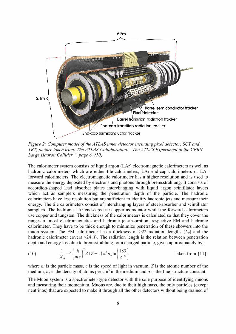
The inner detector consists of a semiconductor pixel detector, a silicon micro-strip detector (SCT) and a transition radiation drift-tube detector (TRT). The pixel- and micro-strip detectors deliver more accurate tracking information but lower hit-rates (~ 3 hits/detector/track). The pixel detector has an accuracy of 10 μm (φ) and 115 μm (z & R) , the SCT has an accuracy of 17 μm (φ) and 580 μm (z & R) . The semiconductor detectors are rather expensive. The TRT is cheaper, could thus be built bigger and delivers more hits per track (~36 hits/track), which compensates for its lower accuracy of ~130 μm (φ) per straw . A precise tracking system is of great importance, especially when dealing with hadron- and heavy-ion collisions which produce a lot more secondary particles than single lepton collisions and thus require more accurate track-reconstruction. The transition radiation allows for a better electron-identification and the precise measurement of the pixel detectors at close proximity to the collision-point allows for primary vertex measurement. In order to enable momentum and charge measurement, the inner detector is immersed in a 2 T strong magnetic field. This field is produced by a toroidal solenoid around the inner detector, which makes it fairly homogeneous and parallel to the beam axis in the barrel-region (less so in the end-cap region). Charge and momentum are measured by determining the handedness and curvature of a track.

(9) F=q (E+v×B)=m v2

R⋅R

One can determine the particle velocity by measuring the particle energy in the calorimeters and subsequently infer the mass using the above equation for the Lorentz-force.

7

Figure 2: Computer model of the ATLAS inner detector including pixel detector, SCT and TRT, picture taken from: The ATLAS-Collaboration: “The ATLAS Experiment at the CERN Large Hadron Collider ”, page 6, {10}

The calorimeter system consists of liquid argon (LAr) electromagnetic calorimeters as well as hadronic calorimeters which are either tile-calorimeters, LAr end-cap calorimeters or LAr forward calorimeters. The electromagnetic calorimeter has a higher resolution and is used to measure the energy deposited by electrons and photons through bremsstrahlung. It consists of accordion-shaped lead absorber plates interchanging with liquid argon scintillator layers which act as samplers measuring the penetration depth of the particle. The hadronic calorimeters have less resolution but are sufficient to identify hadronic jets and measure their energy. The tile calorimeters consist of interchanging layers of steel-absorber and scintillator samplers. The hadronic LAr end-caps use copper as radiator while the forward calorimeters use copper and tungsten. The thickness of the calorimeters is calculated so that they cover the ranges of most electromagnetic- and hadronic jet-absorption, respective EM and hadronic calorimeter. They have to be thick enough to minimize penetration of these showers into the muon system. The EM calorimeter has a thickness of >22 radiation lengths (X0) and the hadronic calorimeter covers >24 X0. The radiation length is the relation between penetration depth and energy loss due to bremsstrahlung for a charged particle, given approximately by:

(10) 1X 0

=4 ( ℏm c )

2

Z (Z+1)α3 na ln( 183

Z1 /3 ) taken from {11}

where m is the particle mass, c is the speed of light in vacuum, Z is the atomic number of the medium, na is the density of atoms per cm3 in the medium and α is the fine-structure constant.

The Muon system is a spectrometer-type detector with the sole purpose of identifying muons and measuring their momentum. Muons are, due to their high mass, the only particles (except neutrinos) that are expected to make it through all the other detectors without being drained of

8

their kinetic energy. Since they are vital in order to determine energy losses in the original collision and to deduce the decay of the primary reactants they have to be identified. Three superconducting toroidal solenoids around the muon system provide a very strong magnetic field which bends the muon path in a circular motion. Within the solenoids four layers of monitored drift tubes (MDT), cathode strip chambers (CSC), resistive plate chambers (RPC) and thin gap chambers (TGC) provide position measurement and triggering.

Important for the later consideration of the ATLAS inner detector is the coordinate system applied to the detector.

• origo = nominal collision point / beam crossing point• positive x-axis points radially towards centre of LHC-ring• positive y-axis points upwards• z axis = beam-axis• azimuthal axis = x-axis• azimuthal angle φ rotates around beam-axis• inclination θ is angle from beam-axis {10}

Figure 3: Computer model of the ATLAS detector including inner detector, EM- and hadronic calorimeters and the muon spectrometer, shows ATLAS coordinate system, picture taken from: The ATLAS-Collaboration: “The ATLAS Experiment at the CERN Large Hadron Collider ”, page 4, {10}

9

Transition Radiation Tracker (TRT)

The ATLAS TRT is a kind of drift-tube detector. The feature that distinguishes it from earlier models is that it consists of drift tubes (straws) which are surrounded by polypropylene fibres and foils. In a conventional drift tube detector, the faster particles traverse it, the lower the interaction cross-section gets and the less ionization-electrons are created in the gas. On the polypropylene surface however, highly relativistic charged particles emit transition-radiation. By passing an interface between two materials with different dielectric permittivity, the particle wave-function has to change homogeneously from one inhomogeneous solution to Maxwell's equations in the first material to another in the second material. The difference in homogeneous and inhomogeneous solution is emitted as transition radiation. The transition radiation intensity is roughly proportional to the particle gamma factor:

(11) I ≈ mrest⋅γ=mrest

√1−( vc )

2 taken from {6}

The transition radiation photons then cause secondary ionisation in the drift tubes. Measuring the charge and ionization-time allows already for a limited momentum, charge and particle identification in the inner tracking detector.

The TRT is made of 298304 straws which are bunched together and arranged so that 52544 of them form a cylinder around the collision point. The straws are oriented parallel to the beam axis and split in the middle forming two segments. Each side of the straw is read out separately so that there are 105088 read-out channels in the barrel-section. One segment stretches from the collision point over the positive part of the beam axis (barrel A) and the other covers the negative part of the beam axis (barrel C). The barrels each have 3 layers, radially stacked on top of each other, counting outwards from 0-6 (0-2 upper half, 3-6 lower half). Each layer is further subdivided into 32 triangular modules per layer and 73 cylindrical straw layers in total.

The other straws are arranged in end-caps A & C each containing 122880 straws. In the end-caps, the straws are oriented orthogonal to the beam axis pointing radially outward from it. Each end-cap consists of 20 wheels (layers) with 8 straw-layers each. That makes 160 consecutive straw layers per end-cap. The layers are counted from the inside-out 0-19.

In the entire detector each straw is made of a carbon-fibre and Aluminium reinforced polimide-tube with an inner diameter of 4 mm. It holds a 31 μm thick gold-plated tungsten wire at its centre. The wire acts as anode and there is an electric potential of –1530V between it and the conductive inner coating of the straw. The used ionization gas mixture is 70% Xe, 27% CO2 and 3% O2. It promotes the detection of low-energy transition radiation photons which allows for better electron-muon distinction and high gain, resulting in more hits.

{5}{7}{8}

10

Figure 4: Section through the ATLAS inner detector showing the position of barrel-sections and end-caps of the pixel detector, SCT and TRT, picture taken from: The ATLAS-Collaboration: “The ATLAS Experiment at the CERN Large Hadron Collider ”, page 54, {10}

Read-out of the 350848 TRT -channels is performed by two subsequent radiation hard chips. The first one (ASDBLR) performs amplification, shaping and baseline restoration and contains two discriminators that register if the energy deposited in the straw exceeds a low threshold of ~250 eV and a high threshold of ~6 keV. The low threshold will be triggered by particles with lower speeds (usually the ones with higher mass due to conservation of momentum, e.g. hadrons), the high threshold is triggered by particles with highly relativistic speeds (low mass, e.g. electrons/positrons) that create a lot of transition radiation. Measuring the threshold is thus an additional (rough) tool for particle identification.

The second chip (DMTROC) measures drift-time. It has 24 bins each of 3.125 ns length so that it covers a total of 75 ns. {2}{9}{8}

Figure 5: working schematic of the TRT front-end electronics, picture taken from: http://www.hep.lu.se/atlas/electronics/trt/electronics_images/trt_electronics_block.gif

11

ProcedureThe analysis and figures that will be presented in the following chapters are based on so called “ntuple-files”. “ntuple-files” contain data dumped from the ATLAS-TRT track-fitter, assigning to each hit registered in the TRT, information about the event number, straw-, chip-, module- and detector-location, which track it belongs to, measured drift-time, drift-radius, unbiased drift-time and drift-radius from the fitted track, calibration constants and all sorts of information about the respective track it was assigned to.

Two datasets were used containing 7.6 GB track data from run 186923 and 10.5 GB from run 187219.

Looping over such large amounts of data requires a simple intermediate or low-level programming language like C++ or perhaps Python. The here used analysis was written by the author in C++ and compiled with GCC 4.6.2 20111027 (Red Hat 4.6.2-1). It utilized the ROOT 5.30/06 analysis framework which was developed by a department at CERN that is uniquely dedicated to the creation of tools for efficient data processing, analysis and storage in high-energy particle physics.

Because looping over the data in one of the files requires about 20 min, the task was split in two parts. First the program (“analysis1.cpp”) fills all required histograms with data from the “ntuple-files” and saves the histograms in a ROOT-tree file. This step has to be performed only once for each dataset. Then a number of other programs import the histograms and common variables from the tree file and further process and plot the data, each focusing on another aspect of the analysis. Because reading histograms goes rather fast the second step can be repeated more often, thus saving time when doing adjustments to the program.

The following C++ programs were used and can be found in the appendix:

• “analysis1.cpp” - program which loops over all track-data, fills and saves histograms and common variables

• “analysis_rt.cpp” - program to fit 3rd degree polynomials to the r-t relation and plot results

• “analysis_res.cpp” - program which finds and plots the time-and space-residuals

• “analysis_nvx.cpp” - program that plots sigma and peak of residuals as function of nvx

• “analysis_tot.cpp” - program that plots the time-residual peak as function of time-over-threshold and nvx

• “analysis_rtnvx.cpp” - program that plots the derivative of the r-t relation at point [18,1] as function of nvx

• “pt_nvx.cpp” - program that plots pt vs. nvx and the mean of pt vs. nvx

12

Calibration of the TRTThe ATLAS-TRT is part of the inner detector, which was predominantly built as tracking device. Hence the most important information gained from the TRT is the reconstruction of all particle paths in spatial coordinates as well as a timing of the same. It is of utmost importance to deliver these quantities as precise as possible in order to later derive the exact point of origin of the particle, its mass, momentum, charge, etc. The straws themselves have a diameter of 4 mm. This spatial uncertainty can be vastly improved upon by measuring drift-time. Drift-time is the time it takes the ionisation-electrons to drift from their point of creation in the straw to the anode wire. The primary electrons get accelerated by the strong, radial electric field between anode-wire and tube wall. They create secondary electrons on the way by scattering on the gas atoms. This avalanche effect only occurs at sufficient electric field strengths. Since the electric field-strength is proportional to the inverse of the distance to the anode wire, this effect only occurs at a distance < 0.2 mm from the anode wire. The avalanche effect further amplifies the signal in a way that the resultant charge depends linearly on field-strength and exponentially on the number of primary electrons and drift length (in the avalanche region).

At distances > 0.2 mm to the wire, the drift-time is almost linearly dependent on drift length. This is because the constant acceleration by the E-field and deceleration by scattering leads to a fairly constant drift-speed that depends on field-strength and the electron mean-free-path in the used gas-mixture. The relation between drift-time and drift-length is called r-t relation. By measuring the drift-time and knowing the r-t relation very well, it is possible to calculate a radius around the anode wire that should in principle have the ionisation-track as tangent. After calculating these radii for all hit straws, one can best-fit a track through the radii which are ideally identical to the original particle track. This method of track reconstruction is used in the ATLAS-TRT and reduces the spatial uncertainty to about 0.12 mm.

The way this uncertainty is determined, is by calculating the time- and space-residuals: Once the 'best fit' track is determined one can calculate its minimum distance to each of the anode-wires at the centre of the straw. This 'ideal drift-length' is compared to the drift length obtained from the measured drift-time and r-t relation. Their absolute difference is the space-residual. Equivalently one can determine an 'ideal drift-time' using the r-t relation and the calculated 'ideal drift-length'. The absolute difference between measured drift-time and calculated drift time constitutes the time-residual. The space- and time-residuals can be determined for each straw. This gives a statistical distribution which should be centred around zero and possess ideally Gaussian shape. The FWHM (Full Width at Half Maximum) of the space-residual and time-residual distributions is defined to be the spatial and temporal resolution of the detector respectively. The calculation of the residuals will be explained more thoroughly in the next two chapters.

13

The r-t relation

The r-t relation is not precisely the same for all straws. Small variations in the making, alignment and front-end electronics of the straws as well as variations in the magnetic field (especially in the end-caps) lead to slightly different relations for every one of the 298304 straws. It is possible to calibrate the r-t relation for every read-out chip, each typically serving 16 straws.

The r-t relation (figure 6) is determined by plotting all hits of a run on a 2-dimensional histogram. Conventionally outliers are then removed from the histogram if the error in drift-radius exceeds 0.5 mm. The histogram is then sliced in vertical slices parallel to the track-to-wire distance axis. Each slice has the width of a histogram-bin (1 ns). Then a Gaussian function is fitted to each slice and the maximum is plotted on a scatter-graph. A 3rd order polynomial can be fitted through the maxima in the scatter-graph which gives the best approximation of the r-t relation.

Figure 6: r-t histogram for run 187219 (entire detector); plotted on top are the maxima of the Gaussian fits to each vertical slice and a 3rd order polynomial fitted to the maxima

However, fitting a Gaussian to these slices might be difficult especially for drift times shorter than 10 ns. If the particle passed close to the anode-wire, the primary ionisation vertexes may lie at very different distances to the anode-wire. This in turn leads to very different drift times and thus a large drift-time uncertainty for short drift-lengths. In addition, for short drift-lengths the ion-velocity does not behave quite as linearly as in the rest of the drift-tube due to the avalanche effect. The result being that slices through the r-t histogram at drift-times below ~10 ns are less Gaussian-shaped. Thus slices below 10 ns are iteratively fitted with a Gaussian in the range of ±0.8×σ to fit the peak more accurately (figure 7), while the slices above 10 ns drift-time are fitted to ±1.5×σ (figure 8).

To later accurately fit the polynomial through the scatter-graph of the peak-positions, an uncertainty has to be associated with each peak. In my analysis this is the χ2 fit-uncertainty of the Gaussian. Formally more correct would be to choose the sigma of the Gaussian. However

14

this uncertainty is way too large and leads to bad fits of the polynomial. In the ATLAS calibration code this is circumvented by a complicated analysis of the variance of the r-t relation under a change of circumstance such as time, run, straw selection, etc. For this analysis the fit-error shall suffice, keeping in mind that at very short and very long drift-times the error is probably larger than shown in the graphs.

Figure 7: slice at drift-time = 6 ns through rt-histogram (see figure ), fitted Gaussian to ±0.8×σ

Figure 8: slice at drift-time = 20 ns through rt-histogram (see figure ), fitted Gaussian to ±1.5×σ

To compare the different r-t relations of different detector sections, the 3rd order polynomials were plotted on the same graph and shifted so that they meet in the point [18 ns,1 mm]. This point was chosen because it lies in the fairly linear central region of the r-t relation which represents the average gradient and has the best statistics (most hits).

Figure 9: 3rd order polynomials obtained from the rt-relations of different detector sections, polynomials are shifted to intersect in point [18,1], run 187219

15

From the above figure the following constants were obtained describing the polynomial:

(12) f (x )=b0+b1⋅x+b2⋅x2+b3 x3

detector section

b0 b1 b2 b3 Derivative at point [18,1]

barrel A 0.0589517 0.0551607 -8.73151e-05 -4.03892e-06 0.0480916

barrel C 0.0589063 0.0552515 -9.49279e-05 -3.88835e-06 0.0480546

inner end-cap A (layer 0-5)

0.0307229 0.0562958 -5.24595e-05 -4.63816e-06 0.0498989

inner end-cap C (layer 0-5)

0.0369077 0.0554797 -1.81009e-05 -5.08879e-06 0.0498818

outer end-cap A (layer 6-13)

0.0148576 0.0543889 0.000158332 -7.743e-06 0.0525626

outer end-cap C (layer 6-13)

0.03427 0.0516473 0.000279416 -9.33683e-06 0.0526309

From figure 9 it is apparent, that for the same track-to-wire distance the electrons drift longest in the barrel region, less long in the inner end-cap region and shortest in the outer end-caps. The magnetic field causes the electron-clusters not to drift directly towards the anode-wire but rather to describe a slight circular motion due to the Lorentz force. Hence the actual drift-length is longer than the perpendicular track-to-wire distance. This circular motion is strongest in the barrel-region where electric field and magnetic field are always orthogonal to each other (Lorentz force acting on electrons is always maximum).

The curvature of the electron path and thus the increase in drift length depends on the angle of the magnetic field in respect to the electric field in the drift-tube. The dependency can be derived from the equation of motion:

(13) m∂ v∂ t

=q ( E+ v×B)−k v (eq. 2.1 in {12})

where m is the electron mass, v is the electron velocity vector, t is time, q is the electron charge, E is the electric field, B is the magnetic field and k is the friction constant of the electrons in the gas.

Since it is known that the electron-velocity is fairly constant in this case, the acceleration due to electric field and the friction can be assumed to balance each other. What remains is the

16

v×B term. This is the force component causing the path curvature. It is proportional to the field strength (|B|) and the sinus of the angle between E-field (nominally v||E) and B-field.

In the end-caps the drift tube is orthogonal to the z-axis. This means that the electric field can be at any angle to the magnetic field, depending on where the track goes through the drift tube. The further out an end-cap wheel lies and the further away the hit is situated from the beam axis, the more the solenoid field is inclined to the plane of the E-field in the tube. Hence statistically drift-times should increase the further out an end-cap is and the further the hit is away from the beam-axis. However the solenoid field also becomes less uniform and thus less strong the further out the end-cap lies. This leads to a smaller curvature and counteracts, apparently dominating the previous effect.

What should be kept in mind from this is that the magnetic field has an influence on the r-t relation and that the position and orientation of the straw tube in the field leads to variations in drift-length. Hence it is advisable to calibrate detector layers or if possible single straws individually.

17

The time- and space-residuals

The time between a triggered event and the first 0→1 transition of the low threshold of a straw-tube is called the leading-edge time (tLE). This is a quantity actually measured in the TRT. It comprises of:

• the time between collision and actual event triggering (tcollision)

• time-of-flight of the particle from the collision to the straw-tube (tToF)

• the time it takes the signal to propagate along the anode wire (tSP)

• drift time of electrons in the straw-tube (t)

The first three quantities are about the same for all straws and thus are combined to the quantity T0. Subtracting T0 from the leading-edge time gives the desired drift-time. In addition two corrections have to be applied: the high-threshold correction and the time-over-threshold correction. They assume a common shape for the charge-time distribution measured at the anode-wire. This allows to correct the leading edge time so that one obtains not the time when the distribution reaches the lower threshold but the actual beginning of the pulse (first root).

Because the signal propagates along the anode wire in both directions and gets reflected off the end which is not connected to the read-out electronics, the detected signal is actually a superposition of two Gaussians. The long tail comes from the slow drift-speed of the positive ions. This gives a pulse shape as shown in figure 10. The pulse-shaper removes the tail to avoid pileup of consecutive pulses.

Figure 10: sketch showing how the ToT- correction value is obtained for a common charge vs time distribution

Figure 11: sketch showing how the HT- correction value is obtained for a common charge vs time distribution

The projected drift-time (ttrackunbias) is the drift-time calculated from a track fit through all hits except the one which the value is being calculated for and the r-t relation. Excluding the current hit from the fit excludes a possible bias if the current hit is an 'outlier' or noise. Subtracting the measured and corrected drift-time from ttrackunbias gives the time-residual.

18

Because the time-residual is the statistical uncertainty of the drift-time measurement, it should be normally distributed and centred around zero. By incrementally changing the calibration constants (T0, HT-correction, ToT-correction) and checking the time- and space-residuals one can minimize their variance and move the peaks to zero. This is the method to verify and optimize the calibration constants.

Figure 12: time-residuals for different detector sections, y-axis drawn normalized, HT and ToT correction are applied, peak and σ determined by iteratively fitting Gaussians to a range of peak ± 1.5 σ, run 187219

From figure 12 it is apparent that the high-threshold residual has a greater uncertainty than the low-threshold one. This is because there are more than two orders of magnitude more low-threshold hits than high-threshold hits. This means there is a much better signal-to-noise ratio for low-threshold hits, which in turn means their r-t relation can be determined with greater accuracy.

19

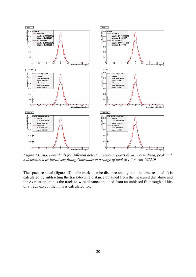
Figure 13: space-residuals for different detector sections, y-axis drawn normalized, peak and σ determined by iteratively fitting Gaussians to a range of peak ± 1.5 σ, run 187219

The space-residual (figure 13) is the track-to-wire distance analogue to the time-residual. It is calculated by subtracting the track-to-wire distance obtained from the measured drift-time and the r-t relation, minus the track-to-wire distance obtained from an unbiased fit through all hits of a track except the hit it is calculated for.

20

The number of primary vertices

An important part of the ATLAS analysis framework “Athena” is the primary vertex reconstruction. This algorithm uses the previously reconstructed tracks and jets of an event to find their common point of origin in the beam-crossing area. This is extremely important because many of the particles ATLAS is looking for are extremely short-lived high-mass particles (H, Z, W, exotics, etc.). These particles will have decayed long before they reach the tracker or calorimeters leaving only secondary decay-products to identify. By tracing the tracks to common clusters of origin one can then infer the nature of the primary particles or perhaps realize where momentum was 'lost' to non-interacting ('invisible') particles.

Because not single protons but rather bunches of protons (~1011 protons/bunch) are collided at the LHC, often several protons will interact in the same bunch crossing.

Multiple short-lived decay-products and the number of p-p interactions per event both contribute to the number of primary vertices (nvx).

Figure 14: dependence of TRT occupance on number of primary vertices, picture taken from: “Public TRT Plots for Collision Data” https://twiki.cern.ch/twiki/bin/view/AtlasPublic/TRTPublicResults {13}

The number of primary vertices can have an effect on the track-fitter performance, because hit-occupancy varies linearly with the number of primary vertices (figure 14).

21

The hit-occupancy is the average number of straws registering a hit divided by the total number of straws for an event. High occupancy thus means it becomes increasingly difficult for the track-fitter to assign single hits to the right track and to recognize and remove noise.

The difference in the slope between data and simulation in figure 14 represents the vertex-finding efficiency. Obviously the vertex finding efficiency is a lot worse for the highest occupancy both in barrel and end-caps than for the lowest occupancy.

Figure 15: distribution of number of hits as function of the number of primary vertices, logarithmic scale, run 187219

For this dataset the number of primary vertices culminates around 5 per event and sufficient statistics to evaluate detector performance exists in the range of approximately 2 ≤ nvx ≤ 11.

22

Figure 16: sigma of time-residual as a function of number of primary vertices, separate for detector sections, no pt-cut, run 187219

Plotting the sigma of the time-residual in this range shows that there is a significant, linear increase of width and thus uncertainty in the drift-time measurement with increasing number of primary vertices. (figure 16) However this is only valid if no pt-cut is introduced.

pt is the transverse momentum - the momentum of particles measured in the x-y plane transverse to the beam axis. Due to conservation of momentum the transverse momentum vectors of all particles originating in the same collision have to cancel each other. Missing pt

in some direction can point to non-interacting particles. If the two protons collide head-on this will usually yield a maximum pt. This also means that a maximum of energy was available for reactions at the collision-point, making high-pt particles generally the more interesting ones. Low pt can be due to edge-on scattering of the protons where only a small fraction of the protons (few partons) was involved in the scattering. This type of collisions will usually lead to jets which retain a high longitudinal momentum, where the risk is high for particles to escape the detector due to a small θ. These events are thus not favoured for further analysis. Low pt can also be because the particles originate from a low-momentum primary collision product, which is not so interesting either.

However, low-momentum particles interact differently with the ionization gas than high-momentum ones. High-momentum particles scatter on single points in the gas (ionization clusters), loosing energy very slowly, retaining most of their momentum and thus also the track direction (unless bent by B-field). The low-momentum particles undergo multiple-scattering, leading to larger deviations from a free-flight path. This makes it impossible for the track-fitter to accurately fit their path, leading to much larger residuals (figure 17). Since low pt particles introduce such large errors they have to be purged from parts of the analysis.

23

A pt-cut at 4 GeV narrowly excludes all those particles with extremely high residuals > 0.118 mm.

Figure 17: dependence of the space-residual width on transverse-momentum, barrel-region, picture taken from: “Public TRT Plots for Collision Data” https://twiki.cern.ch/twiki/bin/view/AtlasPublic/TRTPublicResults {13}

24

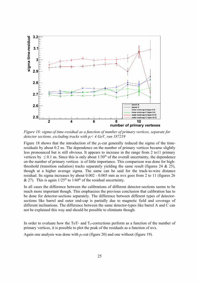
Figure 18: sigma of time-residual as a function of number of primary vertices, separate for detector sections, excluding tracks with pt< 4 GeV, run 187219

Figure 18 shows that the introduction of the pt-cut generally reduced the sigma of the time-residuals by about 0.2 ns. The dependence on the number of primary vertices became slightly less pronounced but is still obvious. It appears to increase in the range from 2 to11 primary vertices by ≤ 0.1 ns. Since this is only about 1/30th of the overall uncertainty, the dependence on the number of primary vertices is of little importance. This comparison was done for high-threshold (transition radiation) tracks separately yielding the same result (figures 24 & 25), though at a higher average sigma. The same can be said for the track-to-wire distance residual. Its sigma increases by about 0.002 - 0.005 mm as nvx goes from 2 to 11 (figures 26 & 27). This is again 1/25th to 1/60th of the residual uncertainty.

In all cases the difference between the calibrations of different detector-sections seems to be much more important though. This emphasizes the previous conclusion that calibration has to be done for detector-sections separately. The difference between different types of detector-sections like barrel and outer end-cap is partially due to magnetic field and coverage of different inclinations. The difference between the same detector-types like barrel A and C can not be explained this way and should be possible to eliminate though.

In order to evaluate how the ToT- and T0-corrections perform as a function of the number of primary vertices, it is possible to plot the peak of the residuals as a function of nvx.

Again one analysis was done with pt-cut (figure 20) and one without (figure 19).

25

Figure 19: peak of time-residual as a function of number of primary vertices, separate for detector sections, no pt-cut, run 187219

Figure 20: peak of time-residual as a function of number of primary vertices, separate for detector sections, excluding tracks with pt< 4 GeV, run 187219

26

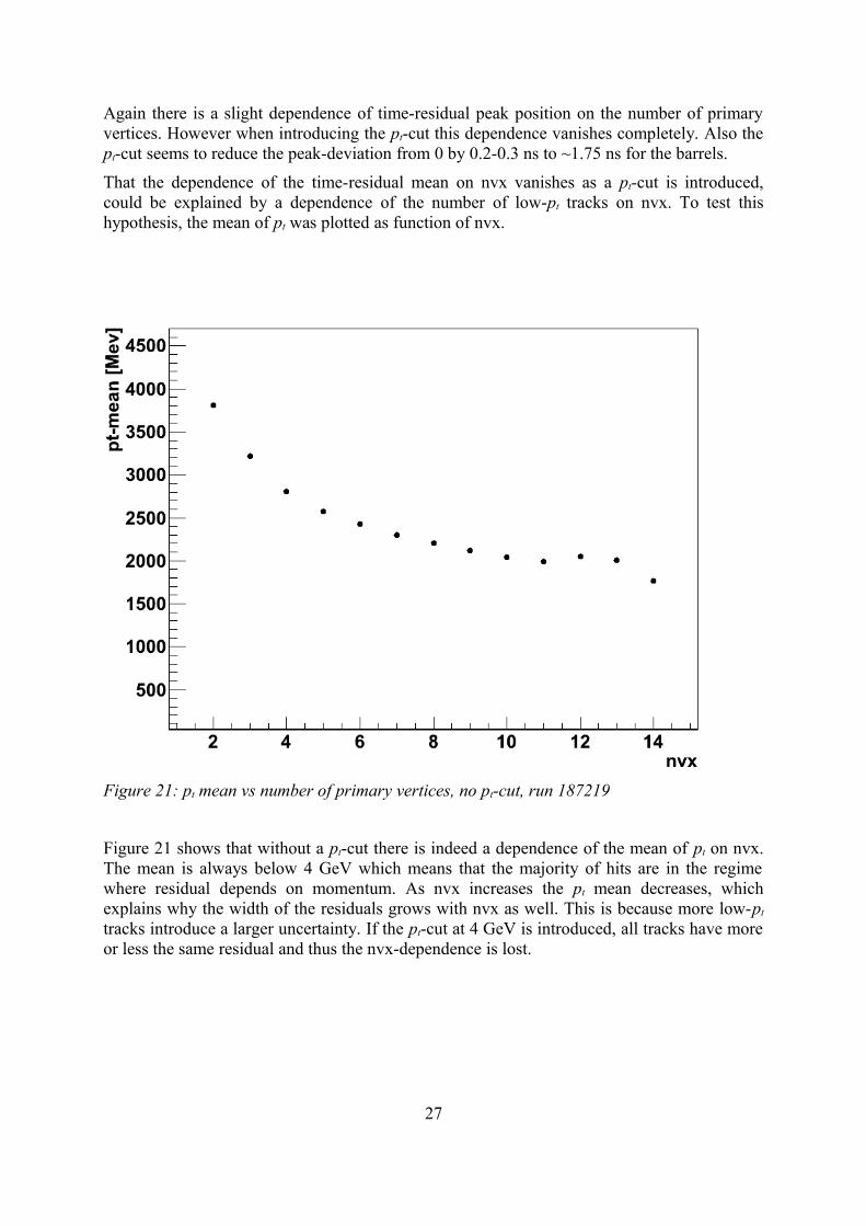
Again there is a slight dependence of time-residual peak position on the number of primary vertices. However when introducing the pt-cut this dependence vanishes completely. Also the pt-cut seems to reduce the peak-deviation from 0 by 0.2-0.3 ns to ~1.75 ns for the barrels.

That the dependence of the time-residual mean on nvx vanishes as a pt-cut is introduced, could be explained by a dependence of the number of low-pt tracks on nvx. To test this hypothesis, the mean of pt was plotted as function of nvx.

Figure 21: pt mean vs number of primary vertices, no pt-cut, run 187219

Figure 21 shows that without a pt-cut there is indeed a dependence of the mean of pt on nvx. The mean is always below 4 GeV which means that the majority of hits are in the regime where residual depends on momentum. As nvx increases the pt mean decreases, which explains why the width of the residuals grows with nvx as well. This is because more low-pt

tracks introduce a larger uncertainty. If the pt-cut at 4 GeV is introduced, all tracks have more or less the same residual and thus the nvx-dependence is lost.

27

Another property one could test against the number of primary vertices is the inclination of the r-t relation in the central section.

Figure 22: first derivative of the r-t relation at point [18,1] as function of the number of primary vertices, no pt-cut, run 187219

The above figure does not reveal any dependence on the number of primary vertices whatsoever and looks the same with a pt-cut introduced.

It is good that there is no such relation, because the number of primary vertices or the transverse-momentum which was previously linked to nvx should not have an influence on the diffusion properties of the detector gas.

28

Performance of the time-over-threshold correction

As explained in the chapter about residuals, the time-over-threshold correction should compensate for a change in ion-pulse shape at different pulse-lengths. The performance of this correction can be readily evaluated by plotting the peak of the time-residual as a function of time-over-threshold.

Figure 23: time-residual mean as a function of time-over-threshold in barrel A, separately plotted for each number of primary vertices, run 187219, pt -cut at pt > 4GeV

Apparently the time-over-threshold correction works best for intermediate pulse-lengths of 8 ns. However in the region of ~ 18 ns the time-residual is shifted by 0.5 to 1 ns. As a reminder: The peak of the time-residual should be at 0. A shifted peak means there is a bias to the error in drift-time measurements. It should be possible to remove this bias by a better calibration of the ToT-correction. In this case the drift-time measurements tend to be longer than projected. The fact that the shift is about the same for each number of primary vertices indicates that this shift is indeed due to the performance of the ToT-correction and has nothing to do with detector occupancy. Because a pt-cut was applied at pt > 4 GeV, the behaviour is not likely to come from the different scattering behaviour of low-momentum tracks, either.

29

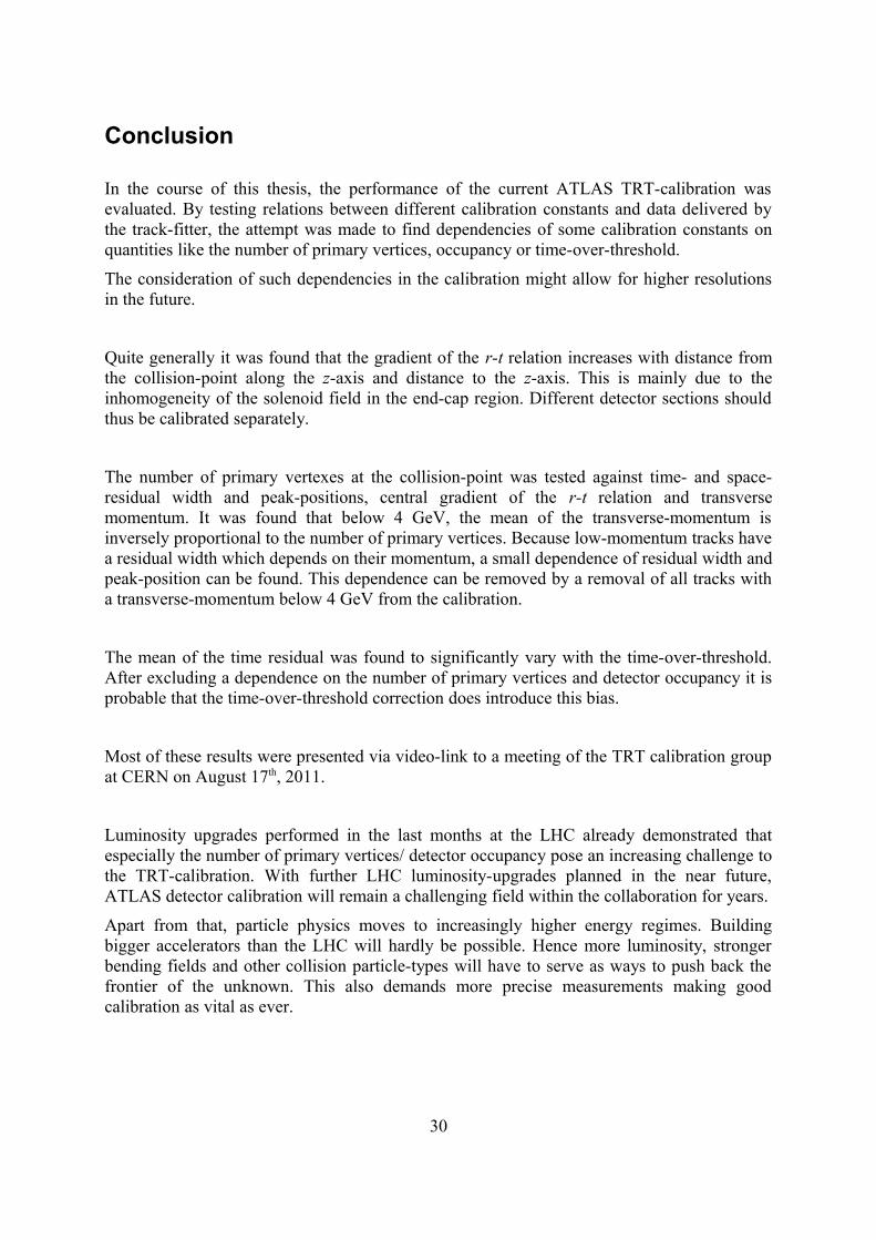
Conclusion

In the course of this thesis, the performance of the current ATLAS TRT-calibration was evaluated. By testing relations between different calibration constants and data delivered by the track-fitter, the attempt was made to find dependencies of some calibration constants on quantities like the number of primary vertices, occupancy or time-over-threshold.

The consideration of such dependencies in the calibration might allow for higher resolutions in the future.

Quite generally it was found that the gradient of the r-t relation increases with distance from the collision-point along the z-axis and distance to the z-axis. This is mainly due to the inhomogeneity of the solenoid field in the end-cap region. Different detector sections should thus be calibrated separately.

The number of primary vertexes at the collision-point was tested against time- and space-residual width and peak-positions, central gradient of the r-t relation and transverse momentum. It was found that below 4 GeV, the mean of the transverse-momentum is inversely proportional to the number of primary vertices. Because low-momentum tracks have a residual width which depends on their momentum, a small dependence of residual width and peak-position can be found. This dependence can be removed by a removal of all tracks with a transverse-momentum below 4 GeV from the calibration.

The mean of the time residual was found to significantly vary with the time-over-threshold. After excluding a dependence on the number of primary vertices and detector occupancy it is probable that the time-over-threshold correction does introduce this bias.

Most of these results were presented via video-link to a meeting of the TRT calibration group at CERN on August 17th, 2011.

Luminosity upgrades performed in the last months at the LHC already demonstrated that especially the number of primary vertices/ detector occupancy pose an increasing challenge to the TRT-calibration. With further LHC luminosity-upgrades planned in the near future, ATLAS detector calibration will remain a challenging field within the collaboration for years.

Apart from that, particle physics moves to increasingly higher energy regimes. Building bigger accelerators than the LHC will hardly be possible. Hence more luminosity, stronger bending fields and other collision particle-types will have to serve as ways to push back the frontier of the unknown. This also demands more precise measurements making good calibration as vital as ever.

30

Sources

Literature

{1} Oxana Smirnova: “Particle Physics – experimental insight”, p.209-214,

lecture notes, Lunds Universitet, 2001

{2} The ATLAS Collaboration: “ATLAS NOTE: Calibration of the ATLAS Transition Radiation Tracker”, ATLAS-CONF-2011-006, February 21st, 2011

{3} David Griffiths: “Introduction to Elementary Particles – Second, Revised Edition”, p. 401-405, Wiley-VCH Verlag, 2008

{4} Gordon Kane: “Modern Elementary Particle Physics – The Fundamental Particles And Forces? - Updated Edition”, Perseus Publishing, 1993

{5} http://www.hep.lu.se/atlas/TRTCalib.html

{6} http://rkb.home.cern.ch/rkb/PH14pp/node194.html

{7} Ben Campbell Smith : “Measurement of the transverse momentum spectrum of W bosons produced at √s = 7 TeV using the ATLAS detector ”, PhD disertation, Harvard University ,Cambridge Massachusetts, May 2011

{8} “The ATLAS Experiment at the CERN Large Hadron Collider ”,

p.59,68-71,76-77, IOP publishing and SISSA , 2008 JINST 3 S08003, 2008

{9} The ATLAS-Collaboration: “ATLAS DETECTOR AND PHYSICS PERFORMANCE – Technical Design Report Volume I” p.10-11,

{10} The ATLAS-Collaboration: “The ATLAS Experiment at the CERN Large Hadron Collider ”, chapt. 1,4,5,6, IOP publishing and SISSA , 2008 JINST 3 S08003, 2008

{11} Oxana Smirnova: “Particle Physics – experimental insight”, p.62, lecture notes, Lunds Universitet, 2001

{12} W. Blum, W. Riegler, L. Rolandi: “Particle Detection with Drift Chambers”, chapter 2, Springer-Verlag, Berlin, Heidelberg, 2008

{13} “Public TRT Plots for Collision Data”

https://twiki.cern.ch/twiki/bin/view/AtlasPublic/TRTPublicResults

{14} http://press.web.cern.ch/press/PressReleases/Releases2011/PR25.11E.html

{15} The ATLAS Collaboration : “Combined search for the Standard Model Higgs boson using up to 4.9 fb−1 of pp collision data at √s = 7 TeV with the ATLAS detector at the LHC ”, arXiv:1202.1408v3 [hep-ex], March 21st, 2012

31

Illustrations

• Figure 1: http://en.wikipedia.org/wiki/File:LHC.svg

• Figure 2: taken from {10} page 6



• Figure 5:

http://www.hep.lu.se/atlas/electronics/trt/electronics_images/trt_electronics_block.gif

• Figure 10 & 11 were created by the author with LibreOffice v3.4.5 Draw

• Figure 14 & 17: taken from {13}

• All other figures were created by the author with ROOT 5.30/06 (http://root.cern.ch ) and C++ compiler: GCC 4.6.2 20111027 (Red Hat 4.6.2-1)

32

Appendix

Additional Figures

Figure 24: sigma of high-threshold time-residual as a function of number of primary vertices, separate for detector sections, no pt-cut, run 187219

Figure 25: sigma of high-threshold time-residual as a function of number of primary vertices, separate for detector sections, excluding tracks with pt< 4 GeV, run 187219

33

Figure 26: sigma of space-residual as a function of number of primary vertices, separate for detector sections, no pt-cut, run 187219

Figure 27: sigma of space-residual as a function of number of primary vertices, separate for detector sections, excluding tracks with pt< 4 GeV, run 187219

34

Figure 28: sigma of high-threshold space-residual as a function of number of primary vertices, separate for detector sections, no pt-cut, run 187219

Figure 29: sigma of high-threshold spacee-residual as a function of number of primary vertices, separate for detector sections, excluding tracks with pt< 4 GeV, run 187219

35

Figure 30: peak of space-residual as a function of number of primary vertices, separate for detector sections, no pt-cut, run 187219

Figure 31: peak of space-residual as a function of number of primary vertices, separate for detector sections, excluding tracks with pt< 4 GeV, run 187219

36

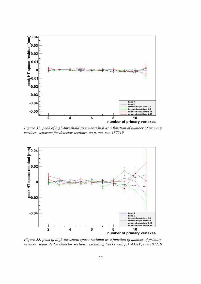
Figure 32: peak of high-threshold space-residual as a function of number of primary vertices, separate for detector sections, no pt-cut, run 187219

Figure 33: peak of high-threshold space-residual as a function of number of primary vertices, separate for detector sections, excluding tracks with pt< 4 GeV, run 187219

37

Figure 34: peak of high-threshold time-residual as a function of number of primary vertices, separate for detector sections, no pt-cut, run 187219

Figure 35: peak of high-threshold time-residual as a function of number of primary vertices, separate for detector sections, excluding tracks with pt< 4 GeV, run 187219

38

Figure 36: transverse-momentum vs. number of primary vertices in the lower pt region, no pt-cut, run 187219

39

Figure 37: time-residual mean as a function of time-over-threshold in barrel A, separately plotted for each number of primary vertices, run 187219, pt -cut at pt > 4GeV

Figure 38: time-residual mean as a function of time-over-threshold in barrel C, separately plotted for each number of primary vertices, run 187219, pt -cut at pt > 4GeV

40

Figure 39: time-residual mean as a function of time-over-threshold in inner end-cap A, separately plotted for each number of primary vertices, run 187219, pt -cut at pt > 4GeV

Figure 40: time-residual mean as a function of time-over-threshold in inner end-cap C, separately plotted for each number of primary vertices, run 187219, pt -cut at pt > 4GeV

41

Figure 41: time-residual mean as a function of time-over-threshold in outer end-cap A, separately plotted for each number of primary vertices, run 187219, pt -cut at pt > 4GeV

Figure 42: time-residual mean as a function of time-over-threshold in outer end-cap C, separately plotted for each number of primary vertices, run 187219, pt -cut at pt > 4GeV

42

Figure 43: time-over-threshold distribution, run 187219, pt -cut at pt > 4GeV

Tube-hits

Tube-hits are by definition hits where the difference between measured track-to-wire distance and track-to-wire distance calculated by the track-fitter exceeds 2.5×σ of the space-residual (~0.5 mm). These hits are considered 'outliers' and are not used for calibration. In the track-fitter their drift-radius measurement is discarded and replaced by the straw-centre position. They are assigned a large error of 4mm/√2 so that they do not bias the track-fitter.The following figures 44-47 show the difference between drift-time and time-residual distribution for tube-hits and non-tube-hits in the region close to the anode-wire where the avalanche effect becomes relevant (changing the r-t relation). Figure 48 shows the tube-hit distribution over the bins of the DTMROC close to the anode-wire. These distributions are as expected and were only created as extra assignment to check how things behave in the avalanche region.Figure 49 shows the distribution of the ratio of tube-hits by total number of hits as a function of primary vertices. This figure is interesting because the fraction of tube-hits can be an indication of track-fitter performance but it bares little relevance to the calibration since tube-hits are generally excluded from the calibration.

43

Figure 44: drift-time distribution (t) for hits close to anode-wire but no tube-hits, no corrections applied, run 187219, no pt -cut

Figure 45: drift-time distribution (t) for hits close to anode-wire but only tube-hits, no corrections applied, run 187219, no pt -cut

44

Figure 46: time-residual distribution for hits close to anode-wire but no tube-hits, run 187219, no pt -cut

Figure 47: time-residual distribution for hits close to anode-wire but only tube-hits, run 187219, no pt -cut

45

Figure 48: time-bin distribution (t+ephase) only for tube-hits, run 187219, no pt -cut

Figure 49: fraction of tube-hits by total number of hits as function of the number of primary vertices, run 187219, no pt -cut

46

Computer code used for the analysis

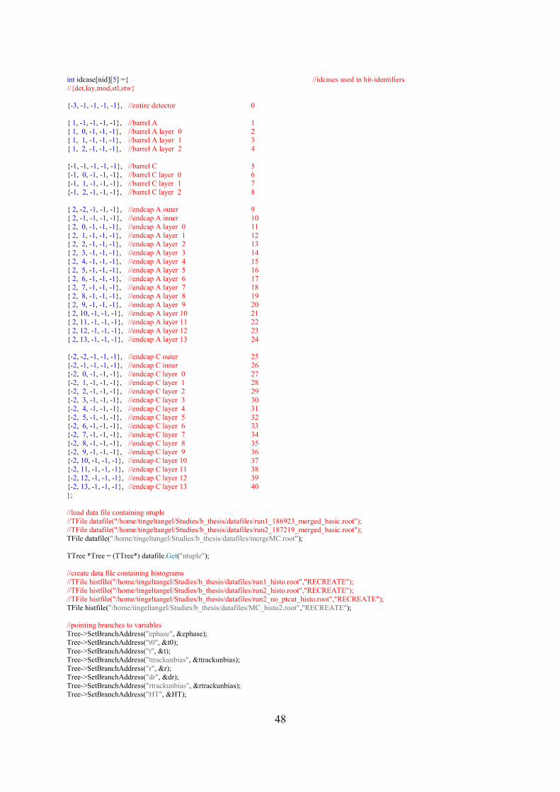
“analysis1.cpp” - program which loops over all track-data, fills and saves histograms and common variables:

#include <math.h> #include <vector> #include <stdio.h> #include <iostream> #include <fstream> #include <string> #include <TH2F.h> #include <TF1.h> #include <TROOT.h> #include <TStyle.h> #include <TChain.h> #include <TFile.h> #include <TTree.h> #include <TCanvas.h> #include <TPad.h> #include <TColor.h> #include <TGraph.h> #include <TGraphErrors.h> #include <TTimeStamp.h> #include <TObjArray.h>

using namespace std;

//###secondary functions###

//###main function### void analysis1(){ //reset CINT gROOT->Reset(); gROOT->SetStyle("Plain"); gStyle->SetOptFit(1111); gStyle->SetPalette(1);

//declare constants const int nid = 41; //# of id cases const float frac = 1; //fraction of data to be read const bool q_htcor = 1; //ht-correction on/off const bool q_totcor = 1; //ToT-correction on/off const bool q_ptcut = 1; //pt-cut on/off const int n_nvx = 14; //max # of primary vertexes to be analyzed

//declare variables TTimeStamp time1; //get starting time float r_drift,t_drift,r_res,t_res; float ephase,t0,t,ttrackunbias,r,dr,rtrackunbias; //variables imported from ntuple float HT,HTCorrection,ToT,ToTCorrection,nvx,pt; //variables imported from ntuple float det, lay, mod, brd, chp; //identifiers imported from ntuple int i,j; //iterators used in loops int iterations; int xbound [3]= {50,0,50}; //bounds of histograms int ybound [3]= {100,0,2}; int rresbound [3]= {200,-2,2}; int tresbound [3]= {200,-20,20}; int totbound [3]= {24,0,75}; //tot bin width is 3.125ns char buf[50]; //textbuffer for naming

vector <TH2F*> rt_vec(nid); //vectors storing histograms vector <TH1F*> rres_vec(nid), tres_vec(nid), htrres_vec(nid), httres_vec(nid); vector <TH2F*> rres_nvx_vec(n_nvx), tres_nvx_vec(n_nvx), htrres_nvx_vec(n_nvx), httres_nvx_vec(n_nvx); vector<vector<TH2F*> > tres_tot_vec(n_nvx,vector<TH2F*>(nid)); vector<vector<TH2F*> > rt_nvx_vec(n_nvx,vector<TH2F*>(nid));

47

int idcase[nid][5] ={ //idcases used in hit-identifiers //{det,lay,mod,stl,stw}

{-3, -1, -1, -1, -1}, //entire detector 0

{ 1, -1, -1, -1, -1}, //barrel A 1 { 1, 0, -1, -1, -1}, //barrel A layer 0 2 { 1, 1, -1, -1, -1}, //barrel A layer 1 3 { 1, 2, -1, -1, -1}, //barrel A layer 2 4

{-1, -1, -1, -1, -1}, //barrel C 5 {-1, 0, -1, -1, -1}, //barrel C layer 0 6 {-1, 1, -1, -1, -1}, //barrel C layer 1 7 {-1, 2, -1, -1, -1}, //barrel C layer 2 8

{ 2, -2, -1, -1, -1}, //endcap A outer 9 { 2, -1, -1, -1, -1}, //endcap A inner 10 { 2, 0, -1, -1, -1}, //endcap A layer 0 11 { 2, 1, -1, -1, -1}, //endcap A layer 1 12 { 2, 2, -1, -1, -1}, //endcap A layer 2 13 { 2, 3, -1, -1, -1}, //endcap A layer 3 14 { 2, 4, -1, -1, -1}, //endcap A layer 4 15 { 2, 5, -1, -1, -1}, //endcap A layer 5 16 { 2, 6, -1, -1, -1}, //endcap A layer 6 17 { 2, 7, -1, -1, -1}, //endcap A layer 7 18 { 2, 8, -1, -1, -1}, //endcap A layer 8 19 { 2, 9, -1, -1, -1}, //endcap A layer 9 20 { 2, 10, -1, -1, -1}, //endcap A layer 10 21 { 2, 11, -1, -1, -1}, //endcap A layer 11 22 { 2, 12, -1, -1, -1}, //endcap A layer 12 23 { 2, 13, -1, -1, -1}, //endcap A layer 13 24

{-2, -2, -1, -1, -1}, //endcap C outer 25 {-2, -1, -1, -1, -1}, //endcap C inner 26 {-2, 0, -1, -1, -1}, //endcap C layer 0 27 {-2, 1, -1, -1, -1}, //endcap C layer 1 28 {-2, 2, -1, -1, -1}, //endcap C layer 2 29 {-2, 3, -1, -1, -1}, //endcap C layer 3 30 {-2, 4, -1, -1, -1}, //endcap C layer 4 31 {-2, 5, -1, -1, -1}, //endcap C layer 5 32 {-2, 6, -1, -1, -1}, //endcap C layer 6 33 {-2, 7, -1, -1, -1}, //endcap C layer 7 34 {-2, 8, -1, -1, -1}, //endcap C layer 8 35 {-2, 9, -1, -1, -1}, //endcap C layer 9 36 {-2, 10, -1, -1, -1}, //endcap C layer 10 37 {-2, 11, -1, -1, -1}, //endcap C layer 11 38 {-2, 12, -1, -1, -1}, //endcap C layer 12 39 {-2, 13, -1, -1, -1}, //endcap C layer 13 40 };

//load data file containing ntuple //TFile datafile("/home/tingeltangel/Studies/b_thesis/datafiles/run1_186923_merged_basic.root"); //TFile datafile("/home/tingeltangel/Studies/b_thesis/datafiles/run2_187219_merged_basic.root"); TFile datafile("/home/tingeltangel/Studies/b_thesis/datafiles/mergeMC.root");

TTree *Tree = (TTree*) datafile.Get("ntuple");

//create data file containing histograms //TFile histfile("/home/tingeltangel/Studies/b_thesis/datafiles/run1_histo.root","RECREATE"); //TFile histfile("/home/tingeltangel/Studies/b_thesis/datafiles/run2_histo.root","RECREATE"); //TFile histfile("/home/tingeltangel/Studies/b_thesis/datafiles/run2_no_ptcut_histo.root","RECREATE"); TFile histfile("/home/tingeltangel/Studies/b_thesis/datafiles/MC_histo2.root","RECREATE");

//pointing branches to variables Tree->SetBranchAddress("ephase", &ephase); Tree->SetBranchAddress("t0", &t0); Tree->SetBranchAddress("t", &t); Tree->SetBranchAddress("ttrackunbias", &ttrackunbias); Tree->SetBranchAddress("r", &r); Tree->SetBranchAddress("dr", &dr); Tree->SetBranchAddress("rtrackunbias", &rtrackunbias); Tree->SetBranchAddress("HT", &HT);

48

Tree->SetBranchAddress("ToT", &ToT); Tree->SetBranchAddress("HTCorrection", &HTCorrection); Tree->SetBranchAddress("ToTCorrection", &ToTCorrection); Tree->SetBranchAddress("pt", &pt); Tree->SetBranchAddress("nvx", &nvx); Tree->SetBranchAddress("det", &det); Tree->SetBranchAddress("lay", &lay); Tree->SetBranchAddress("mod", &mod); Tree->SetBranchAddress("brd", &brd); Tree->SetBranchAddress("chp", &chp);

//create text output-file ofstream ofile; ofile.open ("/home/tingeltangel/Studies/b_thesis/datafiles/rt_output.txt");

//preparing vectors of histograms for(i=0;i<nid;i++){

sprintf(buf,"rt %d",i); rt_vec[i]= new TH2F (buf,buf,xbound[0],xbound[1],xbound[2],ybound[0],ybound[1],ybound[2]); sprintf(buf,"rres %d",i); rres_vec[i]= new TH1F (buf,buf,rresbound[0],rresbound[1],rresbound[2]); sprintf(buf,"tres %d",i); tres_vec[i]= new TH1F (buf,buf,tresbound[0],tresbound[1],tresbound[2]); sprintf(buf,"ht rres %d",i); htrres_vec[i]= new TH1F (buf,buf,rresbound[0],rresbound[1],rresbound[2]); sprintf(buf,"ht tres %d",i); httres_vec[i]= new TH1F (buf,buf,tresbound[0],tresbound[1],tresbound[2]);

}

//preparing vectors of histograms for nvx dependence for(i=0;i<n_nvx;i++){

sprintf(buf,"rres_nvx %d",i); rres_nvx_vec[i]= new TH2F (buf,buf,nid+1,0,nid+1,rresbound[0],rresbound[1],rresbound[2]); sprintf(buf,"tres_nvx %d",i); tres_nvx_vec[i]= new TH2F (buf,buf,nid+1,0,nid+1,tresbound[0],tresbound[1],tresbound[2]); sprintf(buf,"htrres_nvx %d",i); htrres_nvx_vec[i]= new TH2F (buf,buf,nid+1,0,nid+1,rresbound[0],rresbound[1],rresbound[2]); sprintf(buf,"httres_nvx %d",i); httres_nvx_vec[i]= new TH2F (buf,buf,nid+1,0,nid+1,tresbound[0],tresbound[1],tresbound[2]);

//preparing 2d vector for tres vs tot dependence for(j=0;j<nid;j++){ sprintf(buf,"tres_ToT %d %d",i,j); tres_tot_vec[i][j]= new TH2F (buf,buf,totbound[0],totbound[1],totbound[2],tresbound[0],tresbound[1],tresbound[2]);

//preparing 2d vector for dr/dt vs nvx dependence sprintf(buf,"rt_nvx %d %d",i,j); rt_nvx_vec[i][j]= new TH2F (buf,buf,xbound[0],xbound[1],xbound[2],ybound[0],ybound[1],ybound[2]);

}}

//fetch entries from tree and put them into histogram iterations = round(Tree->GetEntries()*frac); for(i=0; i<= iterations; i++){

Tree->GetEntry(i); //remove outliers if ((dr<0.5)&&(pt>4000*q_ptcut)){ //loop over all id-cases for(j=0;j<nid;j++){

if(((idcase[j][0]==det)&&(idcase[j][1]==lay))|| //det fits && lay fits ((idcase[j][0]==det)&&(fabs(idcase[j][0])==1)&&(idcase[j][1]==-1))|| //det fits && det is barrel && lay is

whole barrel ((idcase[j][0]==det)&&(fabs(idcase[j][0])==2)&&(idcase[j][1]==-1)&&(lay<6))| //det fits && det is

endcap && lay is inner endcap ((idcase[j][0]==det)&&(fabs(idcase[j][0])==2)&&(idcase[j][1]==-2)&&(lay>=6))||//det fits && det is endcap && lay is

outer endcap (idcase[j][0]==-3)){ //all detectors together

//calculate drift-time/radius & residuals

49

t_drift = t+ephase-t0-ToTCorrection*q_totcor+HTCorrection*q_htcor; t_res = t+ephase-t0-ttrackunbias-ToTCorrection*q_totcor+HTCorrection*q_htcor; r_drift = fabs(rtrackunbias); r_res = r-rtrackunbias;

//fill r-t histo rt_vec[j]->Fill(t_drift,r_drift); //fill rt histos in respect to nvx if(nvx<=n_nvx){ rt_nvx_vec[nvx-1][j]->Fill(t_drift,r_drift); }

//fill tres vs tot histogram if(nvx<=n_nvx){ tres_tot_vec[nvx-1][j]->Fill(ToT,t_res); }

if(HT){ //fill HT space-residual histograms htrres_vec[j]->Fill(r_res); //fill HT time -residual histograms; httres_vec[j]->Fill(t_res); //fill htrres_nvx and httres_nvx histograms if(nvx<=n_nvx){

htrres_nvx_vec[nvx-1]->Fill(j+0.5,r_res);

httres_nvx_vec[nvx-1]->Fill(j+0.5,t_res); } }else{ //fill space-residual histograms rres_vec[j]->Fill(r_res); //fill time -residual histograms tres_vec[j]->Fill(t_res); //fill rres_nvx and tres_nvx histograms if(nvx<=n_nvx){ rres_nvx_vec[nvx-1]->Fill(j+0.5,r_res); tres_nvx_vec[nvx-1]->Fill(j+0.5,t_res); } }}}}

}

datafile.Close();

//dump histos & constants in root-file i=nid; j=n_nvx; TTree *c_tree = new TTree("c_tree","constants from analysis1"); c_tree->Branch("nid", &i); c_tree->Branch("n_nvx", &j); c_tree->Branch("xbound", xbound,"xbound[3]/I"); c_tree->Branch("ybound", ybound,"ybound[3]/I"); c_tree->Branch("rresbound", rresbound,"rresbound[3]/I"); c_tree->Branch("tresbound", tresbound,"tresbound[3]/I"); c_tree->Branch("totbound", totbound,"totbound[3]/I"); c_tree->Branch("idcase", idcase,"idcase[nid][5]/I"); c_tree->Fill();

histfile.Write(); histfile.Close();

//get & print runtime TTimeStamp time2; cout<<"runtime [min]:"<<(time2.GetSec() - time1.GetSec())/60<<endl;

}

50

“analysis_rt.cpp” - Program to fit 3 rd degree polynomials to the r-t relation and plot results:

#include <math.h> #include <vector> #include <stdio.h> #include <iostream> #include <fstream> #include <string> #include <TH2F.h> #include <TF1.h> #include <TROOT.h> #include <TStyle.h> #include <TChain.h> #include <TFile.h> #include <TTree.h> #include <TCanvas.h> #include <TPad.h> #include <TColor.h> #include <TGraph.h> #include <TGraphErrors.h> #include <TLegend.h>


//###secondary functions### //fit gauss to histogram void itgausfit(TH1F &histo,float &peak,float &peakerror,float &sigma,float &sigmaerror,float &range){

peak = histo.GetMean();//starting-values for iterative gauss fit sigma = histo.GetRMS(); int n = 0; TF1* ffit = new TF1("ffit","gaus"); for(n=0;n<10;n++){

histo.Fit("ffit", "Q","",peak-range*sigma,peak+range*sigma); peak = ffit->GetParameter(1); sigma = ffit->GetParameter(2); n++;

} peak = ffit->GetParameter(1); peakerror = ffit->GetParError(1); sigma = ffit->GetParameter(2); sigmaerror = ffit->GetParError(2); cout<<ffit->GetChisquare()<<endl;

}

//###main function### void analysis_rt() { //reset CINT gROOT->Reset(); gROOT->SetStyle("Plain"); gStyle->SetOptFit(1111); gStyle->SetPalette(1);

//declare constants const int nid = 41; const float polyfix[2] ={18,1}; //point at which rt-fits are shifted to intersect

//declare variables int i,x,y; int xbound [3]; int ybound [3]; int rresbound [3]; int tresbound [3]; int totbound [3]; int idcase[nid][5]; int nslice = 6; //bin no. of the slice which is shown float x_curr;

51

float a0,a1,a2,a3,b0,b1,b2,b3,s; float peak,peakerror,sigma,sigmaerror,range; char buf[50]; char printout[900];

vector <TH2F*> rt_vec(nid); vector <TGraphErrors*> max_vec(nid); vector <TF1*> fitfunc(nid);

TH1F *slice;

//load data file //TFile histfile("/home/tingeltangel/Studies/b_thesis/datafiles/run1_histo.root"); TFile histfile("/home/tingeltangel/Studies/b_thesis/datafiles/run2_histo.root"); //TFile histfile("/home/tingeltangel/Studies/b_thesis/datafiles/run2_no_ptcut_histo.root"); //TFile histfile("/home/tingeltangel/Studies/b_thesis/datafiles/MC_histo.root"); TTree *c_tree = (TTree*) histfile.Get("c_tree");

//set branch addresses & extract variables from tree c_tree->SetBranchAddress("xbound", xbound); c_tree->SetBranchAddress("ybound", ybound); c_tree->SetBranchAddress("rresbound", rresbound); c_tree->SetBranchAddress("tresbound", tresbound); c_tree->SetBranchAddress("totbound", totbound); c_tree->SetBranchAddress("idcase", idcase); c_tree->GetEntry(0);

//fill rtvec with histograms for(i=0;i<nid;i++){

sprintf(buf,"rt %d",i); rt_vec[i] = (TH2F*)histfile.Get(buf); max_vec[i]= new TGraphErrors(); sprintf(buf,"fitfunc %d",i); fitfunc[i]= new TF1(buf,"pol3",xbound[1],xbound[2]);

}

//create canvas TCanvas *canvas1 = new TCanvas("canvas1","rt-histogram",1300,800);

TCanvas *canvas2 = new TCanvas("canvas2","fitted rt's for all detectors",1300,800); TLegend *legend2 = new TLegend(0.1,0.75,0.3,0.9);

TCanvas *canvas3 = new TCanvas("canvas3","rt's for all detectors with errors",1500,800); canvas3->Divide(3,2); TPad* canvas3_1 = (TPad*)(canvas3->GetPrimitive("canvas3_1")); TPad* canvas3_2 = (TPad*)(canvas3->GetPrimitive("canvas3_2")); TPad* canvas3_3 = (TPad*)(canvas3->GetPrimitive("canvas3_3")); TPad* canvas3_4 = (TPad*)(canvas3->GetPrimitive("canvas3_4")); TPad* canvas3_5 = (TPad*)(canvas3->GetPrimitive("canvas3_5")); TPad* canvas3_6 = (TPad*)(canvas3->GetPrimitive("canvas3_6")); TCanvas *canvas4 = new TCanvas("canvas4","slice through rt-histogram",800,600);

//draw rt histo canvas1->cd(); rt_vec[0]->SetXTitle("drift time [ns]"); rt_vec[0]->SetYTitle("track-to-wire distance [mm]"); rt_vec[0]->SetDirectory(0); rt_vec[0]->Draw("COLZ");

//textoutput ofstream ofile; ofile.open ("/home/tingeltangel/Studies/b_thesis/datafiles/rt_output.txt");

//slicing rt histo parallel to y and fitting gauss iteratively to slices TH1F *sliceHisto = new TH1F ("sliceHisto","sliceHisto",ybound[0],ybound[1],ybound[2]);

canvas2->cd();

52

for (i=0; i<nid;i++){ //loop over id-cases for(x=1;x<=xbound[0];x++){ //loop over drift-time bins

for(y=1;y<=ybound[0];y++){ //loop over drift-length bins sliceHisto->SetBinContent(y,rt_vec.at(i)->GetBinContent(x,y));

}

if(sliceHisto->GetEntries() > 0){ //set range for gauss-fit (1.5; 0.8 close to origo) if(x<10){

range = 0.8; }else{

range = 1.5; }

//iteratively fit gaussian to slice itgausfit(*sliceHisto,peak,peakerror,sigma,sigmaerror,range); x_curr = xbound[1]+x*(xbound[2]-xbound[1])/xbound[0]; max_vec[i]->SetPoint(x-1,x_curr,peak); max_vec[i]->SetPointError(x-1,0,peakerror);

} //copy selected slice if((x==nslice)&&(idcase[i][0]==-3)){

slice = (TH1F*)sliceHisto->Clone(); slice->SetName("slice");

}

sliceHisto->Reset(); }

fitfunc[i]->SetLineWidth(1); fitfunc[i]->SetLineColor(kBlack); sprintf(buf,"fitfunc %d",i); max_vec[i]->Fit(buf,"QSame"); max_vec[i]->SetMinimum(ybound[1]); max_vec[i]->SetMaximum(ybound[2]); max_vec[i]->GetHistogram()->GetXaxis()->SetTitle("drift-time [ns]"); max_vec[i]->GetHistogram()->GetYaxis()->SetTitle("track-to-wire distance [mm]");

//maxGraph->SaveAs("/home/tingeltangel/Studies/b_thesis/root_thesis_project/rotplot.root"); //maxGraph->SaveAs("/home/tingeltangel/Studies/b_thesis/root_thesis_project/rotplot_excllow7.root"); sprintf(printout,"id: % 3d % 3d % 3d % 3d % 3d pol3 param: % 5g % 5g % 5g % 5g entries: % 5g",idcase[i]

[0],idcase[i][1],idcase[i][2],idcase[i][3],idcase[i][4],fitfunc[i]->GetParameter(0),fitfunc[i]->GetParameter(1),fitfunc[i]->GetParameter(2),fitfunc[i]->GetParameter(3),rt_vec[i]->GetEntries());

ofile <<printout<<endl; }

//create canvas with rt-fits for inner & outer endcaps as well as barrels canvas2->cd(); fitfunc[1]->SetLineColor(kBlue-4); fitfunc[1]->Draw(); fitfunc[5]->SetLineColor(kBlue+2); fitfunc[5]->Draw("Same"); fitfunc[10]->SetLineColor(kGreen-4); fitfunc[10]->Draw("Same"); fitfunc[26]->SetLineColor(kGreen+2); fitfunc[26]->Draw("Same"); fitfunc[9]->SetLineColor(kRed-4); fitfunc[9]->Draw("Same"); fitfunc[25]->SetLineColor(kRed+2); fitfunc[25]->Draw("Same");

legend2->SetHeader("pol3 fits shiftet to pass [18,1]"); legend2->AddEntry(fitfunc[ 1],"barrel A","L"); legend2->AddEntry(fitfunc[ 5],"barrel C","L"); legend2->AddEntry(fitfunc[10],"inner endcap A","L"); legend2->AddEntry(fitfunc[26],"inner endcap C","L"); legend2->AddEntry(fitfunc[ 9],"outer endcap A","L");

53

legend2->AddEntry(fitfunc[25],"outer endcap C","L"); legend2->Draw();

//create canvas with rtfits with errors canvas3_1->cd(); max_vec[1]->Draw("A*"); max_vec[1]->SetMarkerStyle(1); max_vec[1]->SetTitle("barrel A"); canvas3_4->cd(); max_vec[5]->Draw("A*"); max_vec[5]->SetMarkerStyle(1); max_vec[5]->SetTitle("barrel C"); canvas3_3->cd(); max_vec[9]->Draw("A*"); max_vec[9]->SetMarkerStyle(1); max_vec[9]->SetTitle("outer endcap A"); canvas3_2->cd(); max_vec[10]->Draw("A*"); max_vec[10]->SetMarkerStyle(1); max_vec[10]->SetTitle("inner endcap A"); canvas3_6->cd(); max_vec[25]->Draw("A*"); max_vec[25]->SetMarkerStyle(1); max_vec[25]->SetTitle("outer endcap C"); canvas3_5->cd(); max_vec[26]->Draw("A*"); max_vec[26]->SetMarkerStyle(1); max_vec[26]->SetTitle("inner endcap C");

//shifting rt-functions on canvas 2 so that they meet in polyfix={18,1} for(i=0;i<nid;i++){

a0= fitfunc[i]->GetParameter(0); a1= fitfunc[i]->GetParameter(1); a2= fitfunc[i]->GetParameter(2); a3= fitfunc[i]->GetParameter(3);

s= fitfunc[i]->GetX(polyfix[1],xbound[1],xbound[2])-polyfix[0]; b0= a0+a1*s+a2*pow(s,2)+a3*pow(s,3); b1= a1+2*s*a2+3*pow(s,2)*a3; b2= a2+3*s*a3; b3= a3; cout<<"fitfunc"<<i<<" b0:"<<b0<<" b1:"<<b1<<" b2:"<<b2<<" b3:"<<b3;

fitfunc[i]->SetParameter(0,b0); fitfunc[i]->SetParameter(1,b1); fitfunc[i]->SetParameter(2,b2); fitfunc[i]->SetParameter(3,b3); fitfunc[i]->GetHistogram()->GetXaxis()->SetTitle("drift-time [ns]"); fitfunc[i]->GetHistogram()->GetYaxis()->SetTitle("track-to-wire distance [mm]");

cout<<" derivative at [18,1]"<<fitfunc[i]->Derivative(polyfix[0])<<endl; }

//draw selected slice canvas4->cd(); slice->SetDirectory(0); slice->Draw(); slice->GetXaxis()->SetTitle("track-to-wire distance [mm]"); slice->GetYaxis()->SetTitle("# of hits");

//draw fit plot on color histo canvas1->cd(); max_vec[0]->Draw("PSame");

}

54

“analysis_res.cpp” - Program which finds and plots the time-and space-residuals:





histo.Fit("ffit", "NQ","",peak-range*sigma,peak+range*sigma); peak = ffit->GetParameter(1); sigma = ffit->GetParameter(2); n++;

} peak = ffit->GetParameter(1); peakerror = ffit->GetParError(1); sigma = ffit->GetParameter(2); sigmaerror = ffit->GetParError(2); cout<<ffit->GetChisquare()<<endl;

}

//###main function### void analysis_res() { //reset CINT gROOT->Reset(); gROOT->SetStyle("Plain"); gStyle->SetOptFit(1111); gStyle->SetOptStat(0); gStyle->SetPalette(1);

//declare constants const int nid = 41;

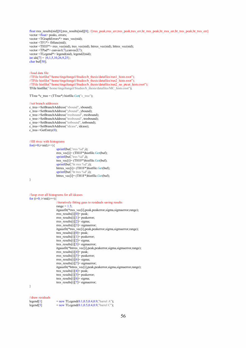
//declare variables int i; int xbound [3]; int ybound [3]; int rresbound [3]; int tresbound [3]; int totbound [3]; int idcase[nid][5]; float peak,peakerror,sigma,sigmaerror,range;

55

float rres_results[nid][8],tres_results[nid][8]; //[rres_peak,rres_err,tres_peak,tres_err,ht_rres_peak,ht_rres_err,ht_tres_peak,ht_tres_err] vector <float> peaks, errors; vector <TGraphErrors*> max_vec(nid); vector <TF1*> fitfunc(nid); vector <TH1F*> rres_vec(nid), tres_vec(nid), htrres_vec(nid), httres_vec(nid); vector <TPad*> canvas1(7),canvas2(7); vector <TLegend*> legend(nid), legend2(nid); int ids[7] = {0,1,5,10,26,9,25}; char buf[50];

//load data file //TFile histfile("/home/tingeltangel/Studies/b_thesis/datafiles/run1_histo.root"); //TFile histfile("/home/tingeltangel/Studies/b_thesis/datafiles/run2_histo.root"); //TFile histfile("/home/tingeltangel/Studies/b_thesis/datafiles/run2_no_ptcut_histo.root"); TFile histfile("/home/tingeltangel/Studies/b_thesis/datafiles/MC_histo.root");

TTree *c_tree = (TTree*) histfile.Get("c_tree");

//set branch addresses c_tree->SetBranchAddress("xbound", xbound); c_tree->SetBranchAddress("ybound", ybound); c_tree->SetBranchAddress("rresbound", rresbound); c_tree->SetBranchAddress("tresbound", tresbound); c_tree->SetBranchAddress("totbound", totbound); c_tree->SetBranchAddress("idcase", idcase); c_tree->GetEntry(0);

//fill rtvec with histograms for(i=0;i<nid;i++){

sprintf(buf,"rres %d",i); rres_vec[i]= (TH1F*)histfile.Get(buf); sprintf(buf,"tres %d",i); tres_vec[i]= (TH1F*)histfile.Get(buf); sprintf(buf,"ht rres %d",i); htrres_vec[i]= (TH1F*)histfile.Get(buf); sprintf(buf,"ht tres %d",i); httres_vec[i]= (TH1F*)histfile.Get(buf);

}

//loop over all histograms for all idcases for (i=0; i<nid;i++){

//iteratively fitting gaus to residuals saving results range = 1.5; itgausfit(*rres_vec[i],peak,peakerror,sigma,sigmaerror,range); rres_results[i][0]= peak; rres_results[i][1]= peakerror; rres_results[i][2]= sigma; rres_results[i][3]= sigmaerror; itgausfit(*tres_vec[i],peak,peakerror,sigma,sigmaerror,range); tres_results[i][0]= peak; tres_results[i][1]= peakerror; tres_results[i][2]= sigma; tres_results[i][3]= sigmaerror; itgausfit(*htrres_vec[i],peak,peakerror,sigma,sigmaerror,range); rres_results[i][4]= peak; rres_results[i][5]= peakerror; rres_results[i][6]= sigma; rres_results[i][7]= sigmaerror; itgausfit(*httres_vec[i],peak,peakerror,sigma,sigmaerror,range); tres_results[i][4]= peak; tres_results[i][5]= peakerror; tres_results[i][6]= sigma; tres_results[i][7]= sigmaerror;

}

//draw residuals legend[1] = new TLegend(0.1,0.5,0.4,0.9,"barrel A"); legend[5] = new TLegend(0.1,0.5,0.4,0.9,"barrel C");

56

legend[10] = new TLegend(0.1,0.5,0.4,0.9,"inner endcap A (layer 0-5)"); legend[26] = new TLegend(0.1,0.5,0.4,0.9,"inner endcap C (layer 0-5)"); legend[9] = new TLegend(0.1,0.5,0.4,0.9,"outer endcap A (layer 6-13)"); legend[25] = new TLegend(0.1,0.5,0.4,0.9,"outer endcap C (layer 6-13)"); legend2[1] = new TLegend(0.1,0.5,0.4,0.9,"barrel A"); legend2[5] = new TLegend(0.1,0.5,0.4,0.9,"barrel C"); legend2[10] = new TLegend(0.1,0.5,0.4,0.9,"inner endcap A (layer 0-5)"); legend2[26] = new TLegend(0.1,0.5,0.4,0.9,"inner endcap C (layer 0-5)"); legend2[9] = new TLegend(0.1,0.5,0.4,0.9,"outer endcap A (layer 6-13)"); legend2[25] = new TLegend(0.1,0.5,0.4,0.9,"outer endcap C (layer 6-13)");

TCanvas *canv1 = new TCanvas("canv1","track-to-wire distance residuals",800,1000); canv1->Divide(2,3); TCanvas *canv2 = new TCanvas("canv2","drift-time residuals",800,1000); canv2->Divide(2,3); for(i=1;i<=6;i++){

sprintf(buf,"canv1_%d",i); canvas1[i] = (TPad*) (canv1->GetPrimitive(buf)); sprintf(buf,"canv2_%d",i); canvas2[i] = (TPad*) (canv2->GetPrimitive(buf)); }

for(i=1;i<=6;i++){ canvas1[i]->cd();

rres_vec[ids[i]]->SetXTitle("r-r_trackunbias [mm]"); rres_vec[ids[i]]->SetYTitle("normalized # of hits");

rres_vec[ids[i]]->SetDirectory(0); rres_vec[ids[i]]->SetLineColor(kRed-4); rres_vec[ids[i]]->DrawNormalized();

htrres_vec[ids[i]]->SetDirectory(0); htrres_vec[ids[i]]->SetLineColor(kRed+2); htrres_vec[ids[i]]->DrawNormalized("Same");

legend[ids[i]]->AddEntry(rres_vec[ids[i]],"residual","L"); sprintf(buf,"peak: % 5g",rres_results[ids[i]][0]); legend[ids[i]]->AddEntry(rres_vec[ids[i]],buf,""); sprintf(buf,"sigma: % 5g",rres_results[ids[i]][2]); legend[ids[i]]->AddEntry(rres_vec[ids[i]],buf,""); legend[ids[i]]->AddEntry(htrres_vec[ids[i]],"HT residual","L"); sprintf(buf,"peak: % 5g",rres_results[ids[i]][4]); legend[ids[i]]->AddEntry(htrres_vec[ids[i]],buf,""); sprintf(buf,"sigma: % 5g",rres_results[ids[i]][6]); legend[ids[i]]->AddEntry(htrres_vec[ids[i]],buf,""); legend[ids[i]]->Draw();

canvas2[i]->cd();

tres_vec[ids[i]]->SetXTitle("T0-T_trackunbias + HT & ToT correction [ns]"); tres_vec[ids[i]]->SetYTitle("normalized # of hits");

tres_vec[ids[i]]->SetDirectory(0); tres_vec[ids[i]]->SetLineColor(kGreen-4); tres_vec[ids[i]]->DrawNormalized();

httres_vec[ids[i]]->SetDirectory(0); httres_vec[ids[i]]->SetLineColor(kGreen+2); httres_vec[ids[i]]->DrawNormalized("Same");

legend2[ids[i]]->AddEntry(tres_vec[ids[i]],"time-residual","L"); sprintf(buf,"peak: % 5g",tres_results[ids[i]][0]); legend2[ids[i]]->AddEntry(tres_vec[ids[i]],buf,""); sprintf(buf,"sigma: % 5g",tres_results[ids[i]][2]); legend2[ids[i]]->AddEntry(tres_vec[ids[i]],buf,""); legend2[ids[i]]->AddEntry(httres_vec[ids[i]],"HT time-residual","L"); sprintf(buf,"peak: % 5g",tres_results[ids[i]][4]); legend2[ids[i]]->AddEntry(httres_vec[ids[i]],buf,""); sprintf(buf,"sigma: % 5g",tres_results[ids[i]][6]); legend2[ids[i]]->AddEntry(httres_vec[ids[i]],buf,""); legend2[ids[i]]->Draw();

57

} }

“analysis_nvx.cpp” - Program that plots sigma and peak of residuals as function of nvx:






} peak = ffit->GetParameter(1); peakerror = ffit->GetParError(1); sigma = ffit->GetParameter(2); sigmaerror = ffit->GetParError(2);

// cout<<ffit->GetChisquare()<<endl;

}

//###main function### void analysis_nvx() { //reset CINT gROOT->Reset(); gROOT->SetStyle("Plain"); gStyle->SetOptFit(1111); gStyle->SetOptStat(0); gStyle->SetPalette(1);

//declare constants const int nid = 41; const int nvxbound [2] = {1,11}; //1<nvx<=12; range of primary vertexes considered

//declare variables int i,j,x,y; int xbound [3]; int ybound [3];

58

int rresbound [3]; int tresbound [3]; int totbound [3]; int idcase[nid][5]; int ids[6] = {1,5,10,26,9,25}; Color_t idscol[6] = {kBlue-4,kBlue+2,kGreen-4,kGreen+2,kRed-4,kRed+2}; float range = 1.5; //fitting gaussian to +- range × sigma float peak,peakerror,sigma,sigmaerror; vector<vector<TGraphErrors*> > max_vec(nid,vector<TGraphErrors*>(8)); vector <vector<TH2F*> > res_nvx_vec(nvxbound[1],vector<TH2F*>(4)); vector <TCanvas*> canvas(8); vector <TH1F*> sliceHisto(4); char buf[50];

//load data file //TFile histfile("/home/tingeltangel/Studies/b_thesis/datafiles/run1_histo.root"); TFile histfile("/home/tingeltangel/Studies/b_thesis/datafiles/run2_histo.root"); //TFile histfile("/home/tingeltangel/Studies/b_thesis/datafiles/run2_no_ptcut_histo.root"); //TFile histfile("/home/tingeltangel/Studies/b_thesis/datafiles/MC_histo.root");



//fill vectors of 2d residual histograms for nvx dependence; [# of prim. vertex][rres,tres,htrres,httres] for(i=nvxbound[0];i<nvxbound[1];i++){

sprintf(buf,"rres_nvx %d",i); res_nvx_vec[i][0]= (TH2F*)histfile.Get(buf); sprintf(buf,"tres_nvx %d",i); res_nvx_vec[i][1]= (TH2F*)histfile.Get(buf); sprintf(buf,"htrres_nvx %d",i); res_nvx_vec[i][2]= (TH2F*)histfile.Get(buf); sprintf(buf,"httres_nvx %d",i); res_nvx_vec[i][3]= (TH2F*)histfile.Get(buf);

}

//create vector of graphs; [detector id][peak rres, sigma rres, peak tres,...] for(i=0;i<nid;i++){

for(j=0;j<8;j++){ max_vec[i][j] = new TGraphErrors();

} }

for(i=0;i<2;i++){ sprintf(buf,"sliceHisto %d",i*2); sliceHisto[i*2] = new TH1F (buf,buf,rresbound[0],rresbound[1],rresbound[2]); sprintf(buf,"sliceHisto %d",i*2+1); sliceHisto[i*2+1] = new TH1F (buf,buf,tresbound[0],tresbound[1],tresbound[2]);

}

//get residuals for all detectors in relation to nvx //loop over all # of primary vertexes for (i=nvxbound[0]; i<nvxbound[1];i++){

//loop over all detector idcases for (x=0;x<nid;x++){

//loop over all y - filling slice histograms for(y=1;y<=rresbound[0];y++){ for(j=0;j<2;j++){ sliceHisto[j*2]->SetBinContent(y,res_nvx_vec[i][j*2]->GetBinContent(x+1,y)); }}

59

for(y=1;y<=tresbound[0];y++){ for(j=0;j<2;j++){ sliceHisto[j*2+1]->SetBinContent(y,res_nvx_vec[i][j*2+1]->GetBinContent(x+1,y)); }} //iteratively fitting gaus to residuals saving results for(j=0;j<2;j++){

itgausfit(*sliceHisto[j*2],peak,peakerror,sigma,sigmaerror,range); max_vec[x][j*4]->SetPoint(i-nvxbound[0],i+1,peak); max_vec[x][j*4]->SetPointError(i-nvxbound[0],0,peakerror); max_vec[x][j*4+1]->SetPoint(i-nvxbound[0],i+1,sigma); max_vec[x][j*4+1]->SetPointError(i-nvxbound[0],0,sigmaerror); itgausfit(*sliceHisto[j*2+1],peak,peakerror,sigma,sigmaerror,range); max_vec[x][j*4+2]->SetPoint(i-nvxbound[0],i+1,peak); max_vec[x][j*4+2]->SetPointError(i-nvxbound[0],0,peakerror); max_vec[x][j*4+3]->SetPoint(i-nvxbound[0],i+1,sigma); max_vec[x][j*4+3]->SetPointError(i-nvxbound[0],0,sigmaerror); sliceHisto[j*2]->Reset(); sliceHisto[j*2+1]->Reset();

} }}

canvas[0] = new TCanvas("canvas1","peak of space residual vs. nvx",1000,800); canvas[1] = new TCanvas("canvas2","sigma of space residual vs. nvx",1000,800); canvas[2] = new TCanvas("canvas3","peak of time residual vs. nvx",1000,800); canvas[3] = new TCanvas("canvas4","sigma of time residual vs. nvx",1000,800); canvas[4] = new TCanvas("canvas5","peak of HT space residual vs. nvx",1000,800); canvas[5] = new TCanvas("canvas6","sigma of HT space residual vs. nvx",1000,800); canvas[6] = new TCanvas("canvas7","peak of HT time residual vs. nvx",1000,800); canvas[7] = new TCanvas("canvas8","sigma of HT time residual vs. nvx",1000,800);

TLegend* legend = new TLegend(0.65,0.1,0.9,0.25,""); legend->AddEntry(max_vec[ids[0]][0],"barrel A","L"); legend->AddEntry(max_vec[ids[1]][0],"barrel C","L"); legend->AddEntry(max_vec[ids[2]][0],"inner end-cap A layer 0-5","L"); legend->AddEntry(max_vec[ids[3]][0],"inner end-cap C layer 0-5","L"); legend->AddEntry(max_vec[ids[4]][0],"outer end-cap A layer 6-13","L"); legend->AddEntry(max_vec[ids[5]][0],"outer end-cap C layer 6-13","L");

max_vec[ids[0]][0]->GetHistogram()->GetYaxis()->SetTitle("peak space-residual [mm]"); max_vec[ids[0]][1]->GetHistogram()->GetYaxis()->SetTitle("sigma space-residual"); max_vec[ids[0]][2]->GetHistogram()->GetYaxis()->SetTitle("peak time-residual [ns]"); max_vec[ids[0]][3]->GetHistogram()->GetYaxis()->SetTitle("sigma time-residual"); max_vec[ids[0]][4]->GetHistogram()->GetYaxis()->SetTitle("peak HT space-residual [mm]"); max_vec[ids[0]][5]->GetHistogram()->GetYaxis()->SetTitle("sigma HT space-residual"); max_vec[ids[0]][6]->GetHistogram()->GetYaxis()->SetTitle("peak HT time-residual [ns]"); max_vec[ids[0]][7]->GetHistogram()->GetYaxis()->SetTitle("sigma HT time-residual");

for(i=0;i<8;i++){ canvas[i]->cd(); max_vec[ids[0]][i]->GetHistogram()->GetXaxis()->SetTitle("number of primary vertexes"); max_vec[ids[0]][i]->SetLineColor(idscol[0]); max_vec[ids[0]][i]->SetMarkerColor(idscol[0]); max_vec[ids[0]][i]->Draw("AL*"); for(j=1;j<6;j++){

max_vec[ids[j]][i]->SetLineColor(idscol[j]); max_vec[ids[j]][i]->SetMarkerColor(idscol[j]); max_vec[ids[j]][i]->Draw("L*");

} legend->Draw();

}

for(i=0;i<nid;i++){ for(j=0;j<8;j++){

max_vec[i][j]->SetMinimum(-10);

60

max_vec[i][j]->SetMaximum(10); }

} }

“analysis_tot.cpp” - Program that plots the time-residual peak as function of time-over-threshold and nvx:






} peak = ffit->GetParameter(1); peakerror = ffit->GetParError(1); sigma = ffit->GetParameter(2); sigmaerror = ffit->GetParError(2);


}

//###main function### void analysis_tot(){ //reset CINT gROOT->Reset(); gROOT->SetStyle("Plain"); gStyle->SetOptFit(1111); gStyle->SetOptStat(0); gStyle->SetPalette(1);

//declare constants const int nid = 41; const int nvxbound [2] = {1,11}; //1<nvx<=12; range of primary vertexes considered

//declare variables int i,j,x,y;

61

Color_t colors[24] = {kPink,kRed,kOrange,kYellow,kSpring,kGreen,kTeal,kCyan,kAzure,kBlue,kViolet,kMagenta,kPink+2,kRed+2,kOrange+2,kYellow+2,kSpring+2,kGreen+2,kTeal+2,kCyan+2,kAzure+2,kBlue+2,kViolet+2,kMagenta+2}; int xbound [3]; int ybound [3]; int rresbound [3]; int tresbound [3]; int totbound [3]; int idcase[nid][5]; int ids[6] = {1,5,10,26,9,25}; //idcases used for graphical output float peak,peakerror,sigma,sigmaerror,range; vector <float> peaks,errors; vector<vector<TH2F*> > trestot_vec(nvxbound[1],vector<TH2F*>(nid)); vector<vector<TGraphErrors*> > max_vec(nvxbound[1],vector<TGraphErrors*>(nid)); vector <TCanvas*> canvas(6); vector <TLegend*> legend(6); char buf[50];

//load data file //TFile histfile("/home/tingeltangel/Studies/b_thesis/datafiles/run1_histo.root"); TFile histfile("/home/tingeltangel/Studies/b_thesis/datafiles/run2_histo.root"); //TFile histfile("/home/tingeltangel/Studies/b_thesis/datafiles/run2_no_ptcut_histo.root"); //TFile histfile("/home/tingeltangel/Studies/b_thesis/datafiles/MC_histo.root"); TTree *c_tree = (TTree*) histfile.Get("c_tree");


//fill vectors with histograms of tres vs tot dependence for(i=nvxbound[0];i<nvxbound[1];i++){

for(j=0;j<nid;j++){ sprintf(buf,"tres_ToT %d %d",i,j); trestot_vec[i][j]= (TH2F*)histfile.Get(buf); max_vec[i][j] = new TGraphErrors();

}}

canvas[0] = new TCanvas("canvas0","tres vs. ToT barrel A",1000,800); canvas[1] = new TCanvas("canvas1","tres vs. ToT barrel C",1000,800); canvas[2] = new TCanvas("canvas2","tres vs. ToT inner endcap A layer 0-5",1000,800); canvas[3] = new TCanvas("canvas3","tres vs. ToT inner endcap C layer 0-5",1000,800); canvas[4] = new TCanvas("canvas4","tres vs. ToT outer endcap A layer 6-13",1000,800); canvas[5] = new TCanvas("canvas5","tres vs. ToT outer endcap C layer 6-13",1000,800);

// slicing rotated histo parallel to y and fitting gauss to slices TH1F *sliceHisto = new TH1F ("sliceHisto","sliceHisto",tresbound[0],tresbound[1],tresbound[2]); //loop over all histograms for all idcases range = 1.5; for (i=nvxbound[0]; i<nvxbound[1];i++){

for(j=0;j<nid;j++){ for(x=1;x<=totbound[0];x++){

for(y=1;y<=tresbound[0];y++){ sliceHisto->SetBinContent(y,trestot_vec[i][j]-

>GetBinContent(x,y)); }

itgausfit(*sliceHisto,peak,peakerror,sigma,sigmaerror,range); max_vec[i][j]->SetPoint(x,x,peak); max_vec[i][j]->SetPointError(x,0,peakerror); sliceHisto->Reset();

}}}

62

legend[0] = new TLegend(0.9,0.5,1,0.9,"barrel A"); legend[1] = new TLegend(0.9,0.5,1,0.9,"barrel C"); legend[2] = new TLegend(0.9,0.5,1,0.9,"inner endcap A layer 0-5"); legend[3] = new TLegend(0.9,0.5,1,0.9,"inner endcap C layer 0-5"); legend[4] = new TLegend(0.9,0.5,1,0.9,"outer endcap A layer 6-13"); legend[5] = new TLegend(0.9,0.5,1,0.9,"outer endcap C layer 6-13");

for(j=0;j<6;j++){ canvas[j]->cd();

for(i=nvxbound[0];i<nvxbound[1];i++){ max_vec[i][ids[j]]->SetLineColor(colors[i]); max_vec[i][ids[j]]->SetMarkerColor(colors[i]); sprintf(buf,"nvx %d",i+1); legend[j]->AddEntry(max_vec[i][ids[j]],buf,"P"); if(i==nvxbound[0]){ max_vec[i][ids[j]]->Draw("AL*"); max_vec[i][ids[j]]->GetHistogram()->GetXaxis()->SetTitle("ToT [ns]"); max_vec[i][ids[j]]->GetHistogram()->GetYaxis()->SetTitle("time residual

[ns]"); max_vec[i][ids[j]]->SetMinimum(-10); max_vec[i][ids[j]]->SetMaximum(10); } max_vec[i][ids[j]]->Draw("L*"); legend[j]->Draw();

}}

}

“analysis_rtnvx.cpp” - program that plots the derivative of the r-t relation at point [18,1] as function of nvx:


using namespace std; //###secondary functions### //fit gauss to histogram void itgausfit(TH1F &histo,float &peak,float &peakerror,float &sigma,float &sigmaerror,float &range){


histo.Fit("ffit", "NQ","",peak-range*sigma,peak+range*sigma); peak = ffit->GetParameter(1); sigma = ffit->GetParameter(2); n++;

} peak = ffit->GetParameter(1); peakerror = ffit->GetParError(1);

63

sigma = ffit->GetParameter(2); sigmaerror = ffit->GetParError(2);


}

//###main function### void analysis_rtnvx() { //reset CINT gROOT->Reset(); gROOT->SetStyle("Plain"); gStyle->SetOptFit(1111); gStyle->SetPalette(1);

//declare constants const int nid = 41; const int nvxbound [2] = {1,11}; //1<nvx<=12; range of primary vertexes considered const float polyfix[2] ={18,1};

//declare variables int i,j,x,y; int xbound [3]; int ybound [3]; int rresbound [3]; int tresbound [3]; int totbound [3]; int idcase[nid][5]; int ids[6] = {1,5,10,26,9,25}; float x_curr; float a0,a1,a2,a3,b0,b1,b2,b3,s; float peak,peakerror,sigma,sigmaerror,range; char buf[50]; Color_t idscol[6] = {kBlue-4,kBlue+2,kGreen-4,kGreen+2,kRed-4,kRed+2};

vector<vector<TH2F*> > rt_nvx_vec(nvxbound[1],vector<TH2F*>(nid)); vector<vector<TGraphErrors*> > max_vec(nvxbound[1],vector<TGraphErrors*>(nid)); vector<vector<TF1*> > fitfunc(nvxbound[1],vector<TF1*>(nid)); vector<TGraphErrors*> drdt_vec(nid);

//load data file //TFile histfile("/home/tingeltangel/Studies/b_thesis/datafiles/run1_histo.root"); //TFile histfile("/home/tingeltangel/Studies/b_thesis/datafiles/run2_histo.root"); TFile histfile("/home/tingeltangel/Studies/b_thesis/datafiles/run2_no_ptcut_histo.root"); //TFile histfile("/home/tingeltangel/Studies/b_thesis/datafiles/MC_histo.root");



//fill vectors with histogram pointers for(i=nvxbound[0];i<nvxbound[1];i++){

for(j=0;j<nid;j++){ //preparing 2d vector for dr/dt vs nvx dependence sprintf(buf,"rt_nvx %d %d",i,j); rt_nvx_vec[i][j]= (TH2F*)histfile.Get(buf); max_vec[i][j] = new TGraphErrors();

64

sprintf(buf,"fitfunc %d %d",i,j); fitfunc[i][j] = new TF1(buf,"pol3",xbound[1],xbound[2]);

} }

for(i=0;i<nid;i++){ drdt_vec[i]= new TGraphErrors(); }

// slicing rt histo parallel to y and fitting gauss to slices TH1F *sliceHisto = new TH1F ("sliceHisto","sliceHisto",ybound[0],ybound[1],ybound[2]); //loop over all histograms for all idcases for (i=nvxbound[0];i<nvxbound[1];i++){

for(j=0;j<nid;j++){ for(x=1;x<=xbound[0];x++){ for(y=1;y<=ybound[0];y++){ sliceHisto->SetBinContent(y,rt_nvx_vec[i][j]->GetBinContent(x,y)); } if(sliceHisto->GetEntries() > 0){ //set range for gauss-fit (1.5; 0.8 close to origo) if(x<10){

range = 0.8; }else{

range = 1.5; } //iteratively fit gaussian to slice itgausfit(*sliceHisto,peak,peakerror,sigma,sigmaerror,range);

x_curr = xbound[1]+x*(xbound[2]-xbound[1])/xbound[0]; max_vec[i][j]->SetPoint(x-1,x_curr,peak); max_vec[i][j]->SetPointError(x-1,0,peakerror);

} sliceHisto->Reset(); }

fitfunc[i][j]->SetLineWidth(1); fitfunc[i][j]->SetLineColor(kGreen); sprintf(buf,"fitfunc %d %d",i,j); max_vec[i][j]->Fit(buf,"QSame"); max_vec[i][j]->SetMinimum(ybound[1]); max_vec[i][j]->SetMaximum(ybound[2]); max_vec[i][j]->GetHistogram()->GetXaxis()->SetTitle("drift time [ns]"); max_vec[i][j]->GetHistogram()->GetYaxis()->SetTitle("trackt-to-wire distance [mm]");

} }

//shifting rt-functions on canvas 2 so that they meet in polyfix={18,1} for(i=nvxbound[0];i<nvxbound[1];i++){

for(j=0;j<nid;j++){ a0= fitfunc[i][j]->GetParameter(0); a1= fitfunc[i][j]->GetParameter(1); a2= fitfunc[i][j]->GetParameter(2); a3= fitfunc[i][j]->GetParameter(3);

s= fitfunc[i][j]->GetX(polyfix[1],xbound[1],xbound[2])-polyfix[0]; b0= a0+a1*s+a2*pow(s,2)+a3*pow(s,3); b1= a1+2*s*a2+3*pow(s,2)*a3; b2= a2+3*s*a3; b3= a3;

peakerror = max_vec[i][j]->GetErrorY(round(fitfunc[i][j]->GetX(polyfix[1],xbound[1],xbound[2])));

fitfunc[i][j]->SetParameter(0,b0); fitfunc[i][j]->SetParameter(1,b1); fitfunc[i][j]->SetParameter(2,b2);

65

fitfunc[i][j]->SetParameter(3,b3); fitfunc[i][j]->GetHistogram()->GetXaxis()->SetTitle("measured drit time [ns]"); fitfunc[i][j]->GetHistogram()->GetYaxis()->SetTitle("trackt-to-wire distance [mm]");

//get derivative at point polyfix drdt_vec[j]->SetPoint(i-nvxbound[0],i+1,fitfunc[i][j]->Derivative(polyfix[0])); drdt_vec[j]->SetPointError(i-nvxbound[0],0,peakerror);

// cout<<i<<" "<<j<<" "<<fitfunc[i][j]->Derivative(polyfix[0])<<endl; }

}

//create canvas TCanvas *canvas1 = new TCanvas("canvas1","d(rres)/d(tdrift) vs nvx",1300,800); canvas1->cd();

drdt_vec[ids[0]]->SetLineColor(idscol[0]); drdt_vec[ids[0]]->SetMarkerColor(idscol[0]); drdt_vec[ids[0]]->Draw("AL*"); drdt_vec[ids[0]]->GetHistogram()->GetXaxis()->SetTitle("nvx"); drdt_vec[ids[0]]->GetHistogram()->GetYaxis()->SetTitle("d(rres)/d(tdrift) at point [18,1]"); drdt_vec[ids[0]]->SetMinimum(0.04); drdt_vec[ids[0]]->SetMaximum(0.08);

for(i=1;i<6;i++){ drdt_vec[ids[i]]->SetLineColor(idscol[i]); drdt_vec[ids[i]]->SetMarkerColor(idscol[i]); drdt_vec[ids[i]]->Draw("*L");

}

TLegend* legend = new TLegend(0.1,0.75,0.3,0.9); legend->AddEntry(drdt_vec[ids[0]],"barrel A","L"); legend->AddEntry(drdt_vec[ids[1]],"barrel C","L"); legend->AddEntry(drdt_vec[ids[2]],"inner end-cap A layer 0-5","L"); legend->AddEntry(drdt_vec[ids[3]],"inner end-cap C layer 0-5","L"); legend->AddEntry(drdt_vec[ids[4]],"outer end-cap A layer 6-13","L"); legend->AddEntry(drdt_vec[ids[5]],"outer end-cap C layer 6-13","L"); legend->Draw();

}

“pt_nvx.cpp” - Program that plots pt vs. nvx and the mean of pt vs. nvx:

#include <math.h> #include <vector> #include <stdio.h> #include <iostream> #include <fstream> #include <string> #include <TH2F.h> #include <TF1.h> #include <TROOT.h> #include <TStyle.h> #include <TChain.h> #include <TFile.h> #include <TTree.h> #include <TCanvas.h> #include <TPad.h> #include <TColor.h> #include <TGraph.h> #include <TGraphErrors.h> #include <TTimeStamp.h> #include <TObjArray.h>

66

#include <TLegend.h>


//###main function### void pt_nvx(){ //reset CINT gROOT->Reset(); gROOT->SetStyle("Plain"); gStyle->SetOptFit(1111); gStyle->SetPalette(1);

float ephase,t0,t,ttrackunbias,r,dr,rtrackunbias,HT,ToT,HTCorrection,ToTCorrection,nvx,pt; //variables imported from ntuple float det, lay, mod, brd, chp; //identifiers imported from ntuple float frac = 1;

//TFile datafile("/home/tingeltangel/Studies/b_thesis/datafiles/run1_186923_merged_basic.root"); TFile datafile("/home/tingeltangel/Studies/b_thesis/datafiles/run2_187219_merged_basic.root"); //TFile datafile("/home/tingeltangel/Studies/b_thesis/datafiles/mergeMC.root");

TTree *Tree = (TTree*) datafile.Get("ntuple");

//point branches to variables Tree->SetBranchAddress("ephase", &ephase); Tree->SetBranchAddress("t0", &t0); Tree->SetBranchAddress("t", &t); Tree->SetBranchAddress("ttrackunbias", &ttrackunbias); Tree->SetBranchAddress("r", &r); Tree->SetBranchAddress("dr", &dr); Tree->SetBranchAddress("rtrackunbias", &rtrackunbias); Tree->SetBranchAddress("HT", &HT); Tree->SetBranchAddress("ToT", &ToT); Tree->SetBranchAddress("HTCorrection", &HTCorrection); Tree->SetBranchAddress("ToTCorrection", &ToTCorrection); Tree->SetBranchAddress("pt", &pt); Tree->SetBranchAddress("nvx", &nvx); Tree->SetBranchAddress("det", &det); Tree->SetBranchAddress("lay", &lay); Tree->SetBranchAddress("mod", &mod); Tree->SetBranchAddress("brd", &brd); Tree->SetBranchAddress("chp", &chp);

TGraphErrors *mean = new TGraphErrors (); TGraphErrors *meanptcut = new TGraphErrors (); TH2F *histo = new TH2F ("histo","pt vs nvx",14,1,15,600,0,60000); TH2F *histoptcut = new TH2F ("histoptcut","pt vs nvx (ptcut at 4GeV)",14,1,15,600,0,60000);

for(int i =0;i<Tree->GetEntries()*frac;i++){ Tree->GetEntry(i); histo->Fill(nvx,pt); if(pt>4000){

histoptcut->Fill(nvx,pt); }

}

for(int j=1;j<15;j++){ mean->SetPoint(j-1,j,histo->ProjectionY("_py",j,j,"")->GetMean()); meanptcut->SetPoint(j-1,j,histoptcut->ProjectionY("_py",j,j,"")->GetMean());

}

TCanvas* canvas = new TCanvas("canvas1","pt vs nvx distribution",900,800); canvas->cd();

histo->SetXTitle("nvx");

67

histo->SetYTitle("pt [Mev]"); histo->SetDirectory(0); histo->Draw("COLZ");

TCanvas* canvas2 = new TCanvas("canvas2","pt-mean vs nvx distribution",900,800); canvas2->cd();

TLegend* legend = new TLegend(0.7,0.75,0.9,0.9); //legend->SetHeader("mean of pt vs nvx:"); legend->AddEntry(mean,"without pt-cut","P"); legend->AddEntry(meanptcut,"with pt>4GeV","P");

mean->GetHistogram()->GetXaxis()->SetTitle("nvx"); mean->GetHistogram()->GetYaxis()->SetTitle("pt-mean [Mev]"); mean->SetMinimum(0); mean->SetMaximum(20000); mean->Draw("A*"); mean->SetMarkerStyle(20); //meanptcut->Draw("*"); meanptcut->SetMarkerStyle(20); meanptcut->SetMarkerColor(kRed); //legend->Draw(); }

68

Date post:	04-Aug-2018
Category:	Documents
Upload:	vudiep
View:	217 times
Download:	0 times

“Evaluation of the ATLAS Transition Radiation Tracker...

Documents