Not to be quoted without prior reference to the authors Fisheries Research Services Internal Report No 04/03 EVALUATION OF THE SAMPLING AND ANALYTICAL TECHNIQUE FOR THE MEASUREMENT OF INORGANIC NUTRIENTS IN SEA WATER C Shaw, R Fryer, J McKie and L Webster March 2003 Fisheries Research Services Marine Laboratory Victoria Road Aberdeen AB11 9DB
Transcript
Not to be quoted without prior reference to the authors
Fisheries Research Services Internal Report No 04/03
EVALUATION OF THE SAMPLING AND ANALYTICAL TECHNIQUE FOR THE MEASUREMENT OF INORGANIC NUTRIENTS IN SEA WATER
C Shaw, R Fryer, J McKie and L Webster
March 2003
Fisheries Research Services Marine Laboratory Victoria Road Aberdeen AB11 9DB
Evaluation of the Sampling and Analytical Technique
1
EVALUATION OF THE SAMPLING AND ANALYTICAL TECHNIQUE FOR THE MEASUREMENT OF INORGANIC NUTRIENTS IN SEA WATER
C Shaw, R Fryer, J McKie and L Webster
Fisheries Research Services, Marine Laboratory,
375 Victoria Road, Aberdeen, AB11 9DB
SUMMARY 1. The precision of measurements of inorganic nutrient concentrations (total oxidised
nitrogen, phosphate, and silicate) in seawater, obtained using a Rosette sampler and a Skalar SAN+ continuous flow analyser, was evaluated in a series of experiments at different concentrations.
2. Total oxidised nitrogen measurements showed severe problems of drift and shifts in
baseline level. 3. The overall precision of phosphate and silicate measurements was between 3 and
4%. Between-batch analytical variation was the largest component of the overall variance, but within-batch analytical variation and variation due to the use of the Rosette were also important.
4. A separate experiment investigated the carryover between samples during an
analytical run of the Skalar. There was significant carryover for phosphate and silicate. Evidence for any carryover of total oxidised nitrogen was difficult to assess due to the effects of drift and shifts in baseline level.
INTRODUCTION Nutrients such as nitrate, nitrite, silicate and phosphate are essential for primary production. Phytoplankton in the euphotic zone of the sea (the part penetrated by light) require nutrients for healthy growth. Phytoplankton are utilised by zooplankton which in turn support pelagic stocks. Nutrient concentrations vary seasonally, with concentrations being lowest in the spring and highest in winter. Phytoplankton numbers increase in the spring due to the increase in light and temperature and therefore nutrient concentrations decrease. As sunlight and temperature decrease in winter, phytoplankton numbers decrease and nutrient concentrations increase. Anthropogenic discharges over the past century have resulted in the nutrient enrichment of coastal waters. Nutrients can enter the marine environment from a number of sources including domestic waste disposal, agriculture run-off, and atmospheric discharges. Increased nutrient levels can lead to phytoplankton blooms, which can be toxic to marine life, and, to coastal eutrophication where waters have low dissolved oxygen and poor quality.1 The monitoring of nutrients in coastal waters is required under several Directives to help assess the eutrophication status of Scottish waters. The Directives include the OSPAR Common Procedure, the EC Nitrates Directive, the EC Urban Waste Water Treatment Directive (UWWD) and the Water Framework Directive (WFD). The OSPAR Common Procedure requires water bodies to be classified as Non-Problem Areas (NPA), Potential Problem Areas (PPA) or Problem Areas (PA), depending on their eutrophication status.2 The overall aim is to achieve a healthy marine environment where eutrophication does not occur by 2010. In Scotland, all coastlines except the upper Firth of Clyde, the Solway Firth
Evaluation of the Sampling and Analytical Technique
2
and the entire east coast south of Peterhead have been classed as NPAs. OSPAR requested the establishment of the eutrophication status for the whole OSPAR area by 2002.2 However, a revision of the Joint Assessment and Monitoring Programme (JAMP) requires the assessment of the eutrophication status by 2003.3 The UWWD and the Nitrate Directive require the eutrophication status of waters up to the 12 mile limit to be assessed every 4 years. The WFD will require the quality of water bodies to be categorised as High, Good, Moderate, Poor or Bad.4,5 Nutrient concentrations are amongst the physico-chemical quality elements that are required to describe water quality. To achieve a High status nutrient levels must be within background ranges. The target date for achieving a Good or High status for all water bodies is 2015. Nutrient levels are also monitored in oceanic areas. Oceanographers use nutrient data, combined with salinity and temperature measurements, to identify how bodies of water interact and move within our seas.6 The precision and accuracy of nutrient measurements is critical in oceanic waters, where concentrations are much lower than in coastal waters. Highly sensitive and precise techniques are therefore required. The analysis of inorganic nutrients (nitrite, nitrate, phosphate and silicate) in both oceanic and coastal waters is carried out at FRS using a continuous flow analyser (CFA). Normally, total oxidised nitrogen (ToxN), the sum of the nitrate and nitrite, is measured. In oceanic waters, ToxN is effectively the nitrate concentration, since the nitrite concentration is negligible. A Skalar SAN+ CFA was used until recently, but this was regarded as outdated and has now been replaced by a Bran & Luebbe CFA. CFAs were the first automated instruments available for nutrient analysis and were adapted from the manual methods previously used. Several other methods have been used for nutrient analysis, most frequently the Flow Injection Analysis (FIA) which has faster analysis times and requires simpler, less expensive equipment. However, CFA is still the preferred method as limits of detection are lower and peaks are easier to quantify. Achieving adequate precision with the CFA is clearly essential if nutrient measurements are to be fit for purpose. However, the chemical analysis is not the only source of variation in nutrient measurements. In particular, the process by which the nutrient samples are collected and prepared can also introduce variation. At FRS, a Rosette is used to take water samples for nutrient analysis on annual hydrographic cruises to monitor chemical and biological parameters along the Jonsis, Fair Isle Munken and Nolsa Flugga lines (Fig. 1). Any ‘handling’ variation in the use of the sampler bottles in the Rosette or in the taking of subsamples for analysis will add to the overall variation in the nutrient measurements. This report describes a series of experiments to estimate the variance components that contribute to the overall precision of nutrient measurements obtained using the Rosette and the Skalar CFA. As well as estimating the overall precision of nutrient measurements, these experiments help to identify the sources of variation which, if controlled, would lead to the greatest improvement in precision. The typical sampling and chemical procedures used to obtain nutrient measurements are described first, since an understanding of these is necessary to understand the description of the variance component experiments that follows. This report also describes a separate experiment to estimate the instrument carryover associated with the Skalar, an effect that occurs when the residue from one sample contaminates a subsequent sample during an analytical run. Significant carryover is highly undesirable and would require the order of chemical analysis to be incorporated in any statistical analysis of nutrient data. Both the variance component experiments and the carryover experiment were repeated using the new Bran & Luebbe analyser, but these experiments will be reported separately.
Evaluation of the Sampling and Analytical Technique
3
Sampling and Chemical Analysis Procedures This section describes the procedures used to measure nutrient concentrations along the Jonsis, Fair Isle Munken and Nolsa Flugga lines in May 1999 on the FRV Scotia. The few modifications required for the variance component experiments are described later. Sample Collection The Rosette consisted of Seabird SBE 32 standard carousel with 12 sampling positions and a Seabird SBE911 CTD (conductivity, temperature and depth sensor). Water samples were collected by attaching twelve sampler bottles (1.7 l; Ocean Test Equipment Inc) to the carousel, lowering the Rosette to the required depth and filling one or more of the sampler bottles. Typically, samples were taken from several depths in a single deployment or ‘dip’ of the Rosette. Once the Rosette was recovered, sub-sample bottles (250 ml plastic bottles with polypropylene caps) were filled from each sampler bottle. The sub-sample bottles were then left to come to room temperature, after which aliquots (~8 ml) from each sub-sample bottle were transferred into sample cups for chemical analysis. Preparation of Standards Stock standards for individual nutrients were purchased from Aldrich Chemical Company (Gillingham, Dorset, UK) and Merck (Lutterworth, Leicestershire, UK). Mixed calibration standards were prepared in plastic volumetric flasks by dilution of the stock solutions using Low Nutrient Sea Water (LNSW). Determination of ToxN, Phosphate and Silicate in Sea Water ToxN, phosphate and silicate were determined simultaneously in seawater using a Skalar SAN+ autoanalyser. Aliquots of each sample (~8 ml) were aspirated using an auto-sampler and transmitted through the complete system by a peristaltic pump. The sample was split three ways and the pump continuously added the reagents required to each sample stream by means of tubes of a certain internal diameter. Air bubbles were evenly pumped through each stream to reduce inter sample dispersion and improve sample throughput. Once the reaction was complete each stream flowed through a colorimeter with the wavelengths set at 540 nm for ToxN, 880 nm for phosphate and 810 nm for silicate and the concentration determined photometrically. Data was collected as an analogue voltage that was fed through a digitising interface to a computer with the Skalar data processing package Version 6. No sample pre-preparation was required. Total oxidised Nitrogen (ToxN) Samples were diluted with ammonium chloride buffer and pumped through a copper coated cadmium column to reduce nitrate to nitrite.7 The nitrite ion was then coupled with sulphanilamide and napthylethylene-diaminehydrochloride (NEDH) to form a pink coloured diazo complex which was determined colorimetrically at a wavelength of 540 nm.8 Interferences from the sample matrix were electronically corrected by optical measurement at 630 nm. Phosphate A mixed reagent containing ammonium molybdate, 2.5M sulphuric acid and antimony potassium tartrate was added to each sample to form an antimonyphosphomolybdate complex with the orthophosphate in the samples. The complex was then reduced by ascorbic acid at 70oC to give a blue colour, which was determined colorimetrically at a
Evaluation of the Sampling and Analytical Technique
4
wavelength of 880 nm.9 Transmission interferences from the sample matrix were electronically corrected by optical measurement at 500 nm. Silicate Each sample was acidified and mixed with ammonium molybdate to form molybdosilic acid.10 This was then reduced with ascorbic acid to form a blue dye, which was determined colorimetrically at a wavelength of 810 nm.11 Oxalic acid was also added to the flowing stream to avoid phosphate interference.12 Calibration and Quality Control Measures A system suitability standard (highest calibration standard) was analysed each day. Calibration standards, covering the range 0.5 µM to 19.3 µM for nitrate, 0.20 µM to 13.3 µM for silicate and 0.04 µM to 1.65 µM for phosphate were analysed at the start and end of each batch and the responses used to compute the calibration curve. Correlation figures of at least 0.999 were achieved for all nutrients. The limit of detection, based on 4.65 times the standard deviation of the mean value from repeat analysis of ten low standards, was 0.5 µM for nitrate, 0.03 µM for phosphate, 0.2 µM for silicate.13 A laboratory reference material (LRM) was included in each batch of samples. In addition Sagami certified reference materials (CRM), obtained from Promochem Ltd, were analysed once at the start of each day. The data obtained from the CRM and LRM were transferred onto NWA Quality Analyst and Shewhart charts produced with warning and action limits being drawn at ± 2 x and ± 3 x the standard deviation of results. Further quality control was assured through successful participation in the nutrient programme of QUASIMEME (Quality Assurance of Information for Marine Environmental Monitoring in Europe). These methods are accredited by the United Kingdom Accreditation Services (UKAS). Variance Component Experiments Sources of variation The measurement of nutrient concentrations described above has four main potential sources of variation. Two of these are associated with the chemical analysis: the • between-analysis variance 2
analysisσ , the variation between replicate analyses (i.e. between measurements from different aliquots taken from the same sub-sample bottle)
• between-batch variance 2
batchσ , the variation introduced by analysing the same material but in different analytical batches
The other two sources of variation are associated with the use of the Rosette: the • between-bottle variance 2
bottleσ , the variation introduced through the use of sub-sample bottles
• between-sampler variance 2
samplerσ , the variation introduced through the use of sampler bottles
The overall variance of a nutrient measurement 2
nutrientσ is the sum of these four components 22222samplerbottlebatchanalysisnutrient σ+σ+σ+σ=σ
Evaluation of the Sampling and Analytical Technique
5
Of course, there is also a fifth and very important variance component that has nothing to do with the measurement process: • the field variance 2
fieldσ , the natural variation in nutrient concentrations. The precise definition of the field variance will depend on the experimental context. Here it is taken to be the natural variation in nutrient concentrations between different dips of the Rosette at the same nominal position and depth made within the space of a few hours. Experimental design The variance component experiments were designed to estimate 2
analysisσ , 2bottleσ , and 2
samplerσ
and to provide limited information on the combined effect of 2batchσ and 2
fieldσ . Each experiment consisted of five dips with the Rosette at the same nominal position and depth. On each dip, twelve water sampler bottles were attached to the carousel, the Rosette was lowered to the required depth, and the samplers were filled. Once recovered, 9 of the 12 samplers were chosen at random. Two sub-sample bottles were then filled from each of the 9 samplers and labelled a and b; e.g. 1a and 1b if they came from sampler 1, etc. One of each pair of sub-sample bottles was then randomly chosen and labelled with a star; e.g. 1a*. Due to constraints on the total number of analyses possible in any one analytical batch, one of the starred sub-sample bottles was randomly discarded, leaving 17 sub-sample bottles. The sub-sample bottles were then left to come to room temperature, after which two aliquots (~8 ml) from each of the starred sub-sample bottles and one aliquot from each of the non-starred sub-sample bottles were transferred into sample cups for analysis. These 25 cups, combined with those filled with standards and laboratory reference material, filled all 40 positions in the Skalar auto-sampler tray. The sample cups were placed at random in the auto-sampler and analysed. The idea behind the design is that the between-analysis variance 2
analysisσ can be estimated by comparing the nutrient measurements from the different aliquots taken from the same sub-sample bottle. Similarly, the between-bottle variance 2
bottleσ can be estimated by comparing the measurements from different sub-sample bottles but the same sampler. And the between-sampler variance 2
samplerσ can be estimated by comparing the measurements from different samplers but the same dip. The somewhat complex mechanism for choosing samplers, sub-sample bottles and aliquots was necessary, partly because only 40 analyses were possible in each batch, and partly to ensure there were the same number of degrees of freedom for estimating each of 2
analysisσ , 2bottleσ , and 2
samplerσ (eight per dip). For logistic reasons, the samples from each dip were analysed in separate batches of the CFA. This means that 2
batchσ and 2fieldσ could not be estimated separately; only their sum 22
fieldbatch σ+σ was estimable from the data. More information on the chemical variance components 2
analysisσ and 2batchσ was obtained
from the analyses of Certified and Laboratory Reference materials (CRMs and LRMs) that were run randomly during each analytical batch. There were few replicate analyses of the CRMs and LRMs in each batch, so 2
analysisσ and 2batchσ could not be estimated separately;
only their sum 22batchanalysis σ+σ was estimable from the data.
Evaluation of the Sampling and Analytical Technique
6
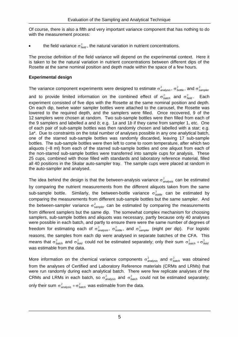
Sample collection and preparation Three variance component experiments were conducted on the FRV Scotia in May 1999. The first two were conducted at depths of 50 and 410 m respectively at a station on the Fair Isle Munken line. The third experiment was at a depth of 900 m from a station in the Rockall trough. The three depths were chosen to provide a range of typical oceanic nutrient concentrations. Inorganic nutrient concentrations usually increase with depth since dead phytoplankton sink from the upper ocean to the sea bed releasing nutrients as they fall. Five dips were made at 50 and 410 m as planned, but only one dip was possible at 900 m. Unfortunately, samples from the fifth dip at 50 m were contaminated through user error. The samples from 50 m took approximately one hour to reach room temperature. However, the samples from 410 m and 900 m were much colder, so were placed in a water bath at 35-40oC for 45 minutes and then left at room temperature for 15 minutes before analysis. Statistical methods The variance components were estimated by residual maximum likelihood, with the constraint that all variances had to be non-negative.14 The significance of the variance components was assessed by likelihood ratio tests. No attempt was made to model the order of chemical analysis to account for the effects of drift. Although this would have been desirable, there is no simple way of modelling the shifts in baseline level that accompany drift. Results The data are plotted in Figures 2 and 3 and estimates of the variance components are given in Tables 1 and 2. ToxN measurements from all three depths showed severe problems of downward drift and shifts in baseline level (approximately ±2 µM) within each analytical batch (i.e. within each dip) (Fig. 2). The downward drift was due to deterioration in the cadmium reduction column.15 The shifts in baseline level occurred as the Skalar software corrected for the drift. The drift and shifts in baseline level were so severe that little can be taken from the variance estimates in Tables 1 and 2. Phosphate and silicate measurements showed no severe problems of drift or shift in baseline level (Fig. 2). Variation in phosphate and silicate measurements was dominated by variation between dips (i.e. the combined effect of 2
batchσ and 2fieldσ ) particularly at 50 m
(Table 1, Fig. 2). This indicates large between-batch variance at low concentrations and / or large field variation at this depth. For phosphate, the between-analysis variance 2
analysisσ , the
between-bottle variance 2bottleσ , and the between-sampler variance 2
samplerσ were all statistically significant (p < 0.05) and, more importantly, of monitoring significance with estimated coefficients of variation of around 1 to 2% (Table 1, Fig. 3). For silicate, the between-bottle variation 2
bottleσ was negligible, but the between-analysis variation 2analysisσ and
between-sampler variation 2samplerσ were both statistically significant (p < 0.05) and of
monitoring significance with estimated coefficients of variation of around 1 to 2% (Table 1, Fig. 3). The estimates in Tables 1 and 2 were combined to estimate 2
batchσ (see Appendix for details) and hence to estimate the overall variance of a nutrient measurement 2
nutrientσ (Table 3). The overall coefficient of variation of phosphate and silicate measurements was between 3 and
Evaluation of the Sampling and Analytical Technique
7
4%. In general, the between-batch analytical variance 2batchσ was the largest component of
the overall variance with an estimated coefficient of variation of between 2.5 and 3.5%. Carryover Experiment Experimental design Water samples were prepared by adding aliquots of concentrated stock solution of each nutrient to Low Nutrient Sea water (LNSW). LNSW is collected from the North Sea in the summer months in 25L plastic carboys and has nutrient concentrations from 0.7–1.5 µM for silicate, 1.7–2.7 µM for ToxN, and 0.10–0.20 µM for phosphate. Two solutions were prepared in plastic volumetric flasks, one at a low concentration of each nutrient (ToxN, 5.0 µM; phosphate, 0.40 µM; and silicate, 4.0 µM) and one at a high concentration (ToxN, 10.0 µM; phosphate, 0.80µM; and silicate, 8.0 µM). The concentrations were chosen so as not to cause any limit of detection problems. 25 aliquots of the low and high concentration solutions were transferred to cups on the auto-sampler in the following manner: aliquot position concentration
1 high 2 low 3 low 4 high 5 high 6 low etc. These were then analysed using the CFA. This process was conducted four times. The idea behind this design was that the measured concentrations of e.g. aliquots 3 and 5 should be unaffected by any carryover effect as they directly follow a solution of the same concentration. However, the measured concentrations of e.g. aliquots 2 and 4 might be affected by carryover as they follow a solution of a different concentration. Therefore, the difference in the measured concentrations of two successive ‘low’ or ‘high’ solutions will be a measure of the carryover effect of moving from high to low concentrations and from low to high respectively. Statistical methods Let bax be the measured concentration from aliquot a in batch b. Then
23226762321 bbbbbbbbb xxyxxyxxy −=−=−= ... , , are the six differences from each batch that provide information on the carryover from high to low concentrations. Similarly,
25246982541 bbbbbbbbb xxzxxzxxz −=−=−= ... , , are the six differences from each batch that provide information on the carryover from low to high concentrations. The derived data biy , i = 1…6, b = 1,2,4,5, and biz , i = 1…6, b = 1,2,4,5, were both assessed for evidence of differences between batches by analysis of variance. No differences were found (p > 0.05) so the data were pooled over batches.
Evaluation of the Sampling and Analytical Technique
8
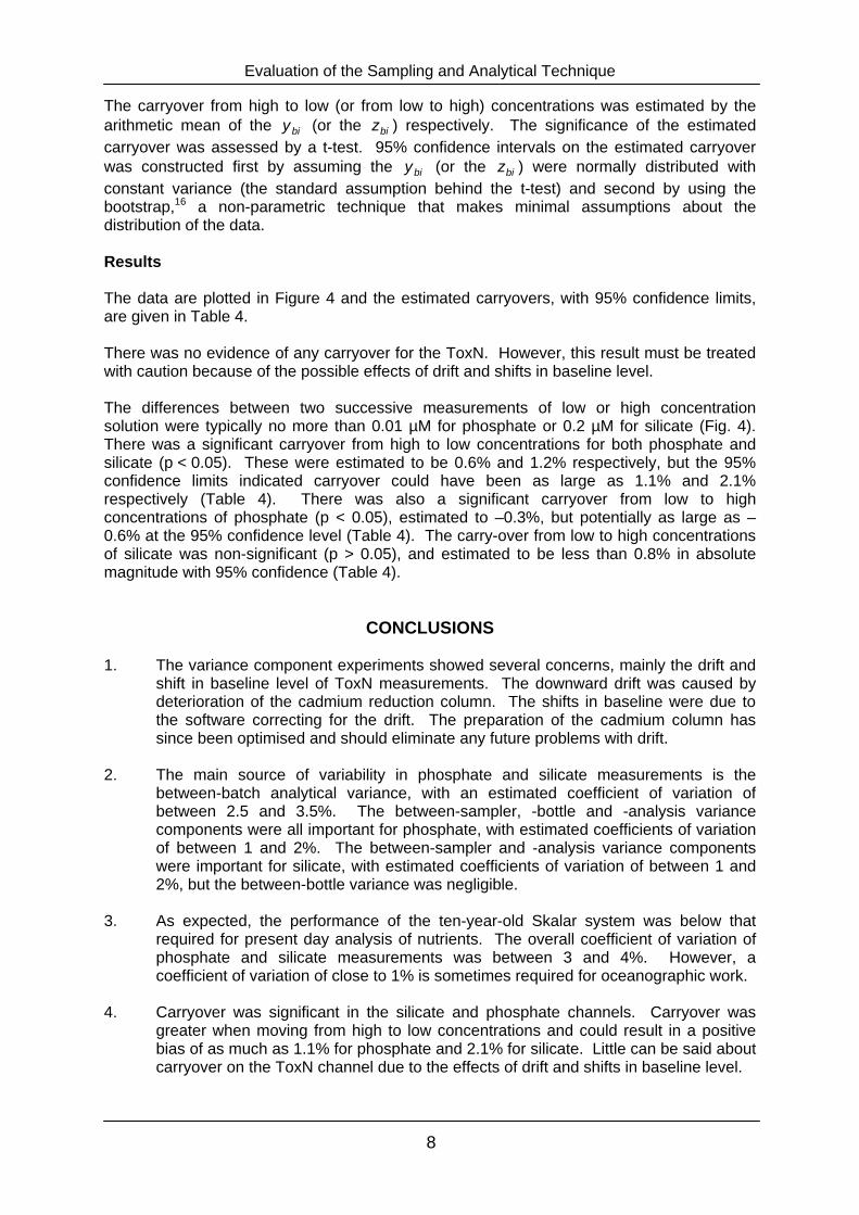
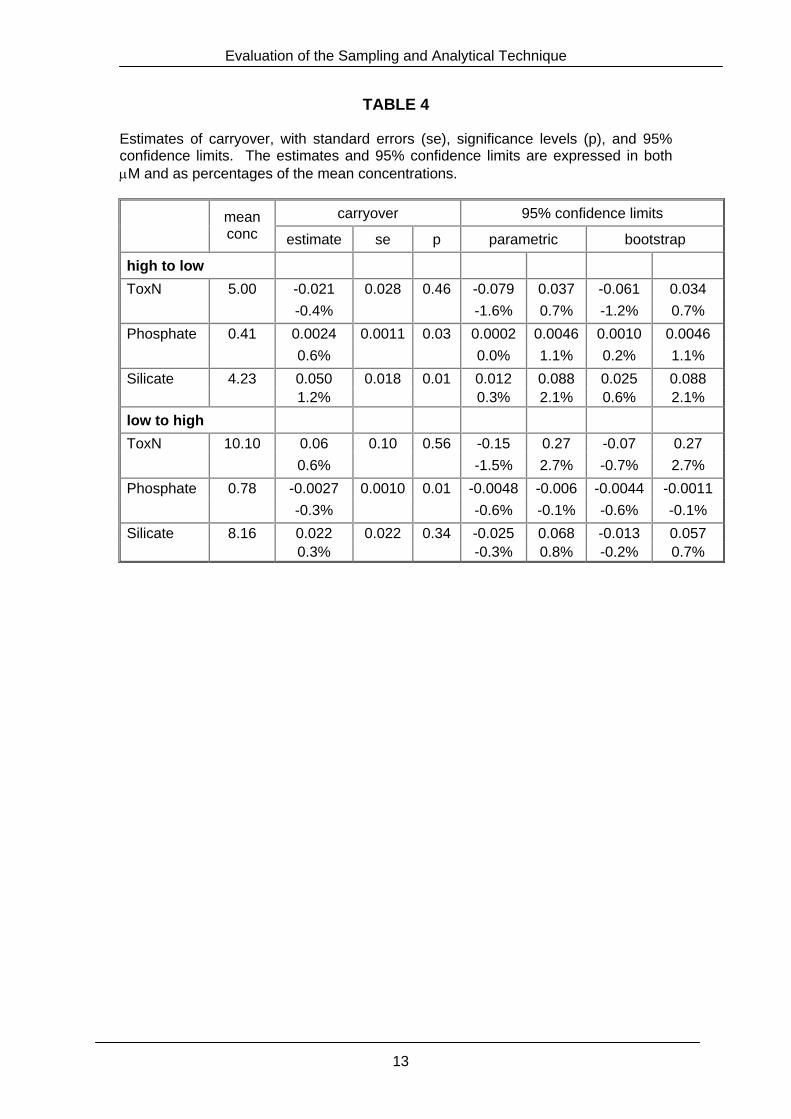
The carryover from high to low (or from low to high) concentrations was estimated by the arithmetic mean of the biy (or the biz ) respectively. The significance of the estimated carryover was assessed by a t-test. 95% confidence intervals on the estimated carryover was constructed first by assuming the biy (or the biz ) were normally distributed with constant variance (the standard assumption behind the t-test) and second by using the bootstrap,16 a non-parametric technique that makes minimal assumptions about the distribution of the data. Results The data are plotted in Figure 4 and the estimated carryovers, with 95% confidence limits, are given in Table 4. There was no evidence of any carryover for the ToxN. However, this result must be treated with caution because of the possible effects of drift and shifts in baseline level. The differences between two successive measurements of low or high concentration solution were typically no more than 0.01 µM for phosphate or 0.2 µM for silicate (Fig. 4). There was a significant carryover from high to low concentrations for both phosphate and silicate (p < 0.05). These were estimated to be 0.6% and 1.2% respectively, but the 95% confidence limits indicated carryover could have been as large as 1.1% and 2.1% respectively (Table 4). There was also a significant carryover from low to high concentrations of phosphate (p < 0.05), estimated to –0.3%, but potentially as large as –0.6% at the 95% confidence level (Table 4). The carry-over from low to high concentrations of silicate was non-significant (p > 0.05), and estimated to be less than 0.8% in absolute magnitude with 95% confidence (Table 4).
CONCLUSIONS 1. The variance component experiments showed several concerns, mainly the drift and
shift in baseline level of ToxN measurements. The downward drift was caused by deterioration of the cadmium reduction column. The shifts in baseline were due to the software correcting for the drift. The preparation of the cadmium column has since been optimised and should eliminate any future problems with drift.
2. The main source of variability in phosphate and silicate measurements is the
between-batch analytical variance, with an estimated coefficient of variation of between 2.5 and 3.5%. The between-sampler, -bottle and -analysis variance components were all important for phosphate, with estimated coefficients of variation of between 1 and 2%. The between-sampler and -analysis variance components were important for silicate, with estimated coefficients of variation of between 1 and 2%, but the between-bottle variance was negligible.
3. As expected, the performance of the ten-year-old Skalar system was below that
required for present day analysis of nutrients. The overall coefficient of variation of phosphate and silicate measurements was between 3 and 4%. However, a coefficient of variation of close to 1% is sometimes required for oceanographic work.
4. Carryover was significant in the silicate and phosphate channels. Carryover was
greater when moving from high to low concentrations and could result in a positive bias of as much as 1.1% for phosphate and 2.1% for silicate. Little can be said about carryover on the ToxN channel due to the effects of drift and shifts in baseline level.
Evaluation of the Sampling and Analytical Technique
9
5. FRS Marine Laboratory has introduced the Bran & Luebbe continuous flow analyser for the determination of nutrients in seawater and data on the variance and carryover will be presented in a separate report.
REFERENCES 1. OSPAR Quality Status Report 2000. Chapter 4-Chemistry. 2. OSPAR Strategy to Combat eutrophication, 1998, 1998-18. 3. OSPAR, The revision of the Joint Assessment and Monitoring Programme (JAMP),
2003, INPUT 03/2/1-E. 4. Water Framework Directive, Directive 2000/60.EC of the European Parliament and of
the Council, 2000. 5. OSPAR, Point of departure for discussions on integrating the OSPAR Common
Procedure and the Water Framework Directive with respect to eutrophication, 2001, ref 5.10c.
6. Redfield A.C, Ketchum B.H and Richards F.A, 1963, The Sea , 2, Wiley-Interscience,
New York, 26-76. 7. Wood, E.D, Armstrong, F.A.J. and Richards, F.A., 1967. Determination of nitrate in
sea water By cadmium copper reduction to nitrite, J. Mar. Biol. Ass. U.K., 47, 23-31.
8. Bendschneider, K. and Robinson, R.J., 1952. A new spectrophotometric method for
the determination of nitrite in sea water, J. Mar. Res., 11, 87. 9. Murphy, J. and Riley, J.P., 1958. J. Mar. Biol. Ass. UK., 37, 9. 10. Atkins, W.R.G., 1923. The silica content of some natural waters and of culture
media, J. Mar. Biol. Ass. U.K, Vol X111, 151-159. 11. Koreloff, F., ICES C.M. 1971/C:43 (mimeo) 12. Armstrong, F. A. J., 1951. The determination of silicate in sea water, J. Mar. Biol.
Ass. U.K., 30, 149. 13. Cheeseman, R.V. and Wilson, A.L., A Manual on Analytical Quality Control For The
Water Industry, 1989, 21. 14. Robinson, D.L., 1987. Estimation and the use of variance components. The
Statistician, 36, 3-14. 15. Garside, C., 1993. Nitrate reductor efficiency as an error source in seawater
analysis, Mar. Chem., 44, 25-30. 16. Efron, B. and Tibishirani, R.J., 1993. An Introduction to the bootstrap. Chapman
and Hall. New York.
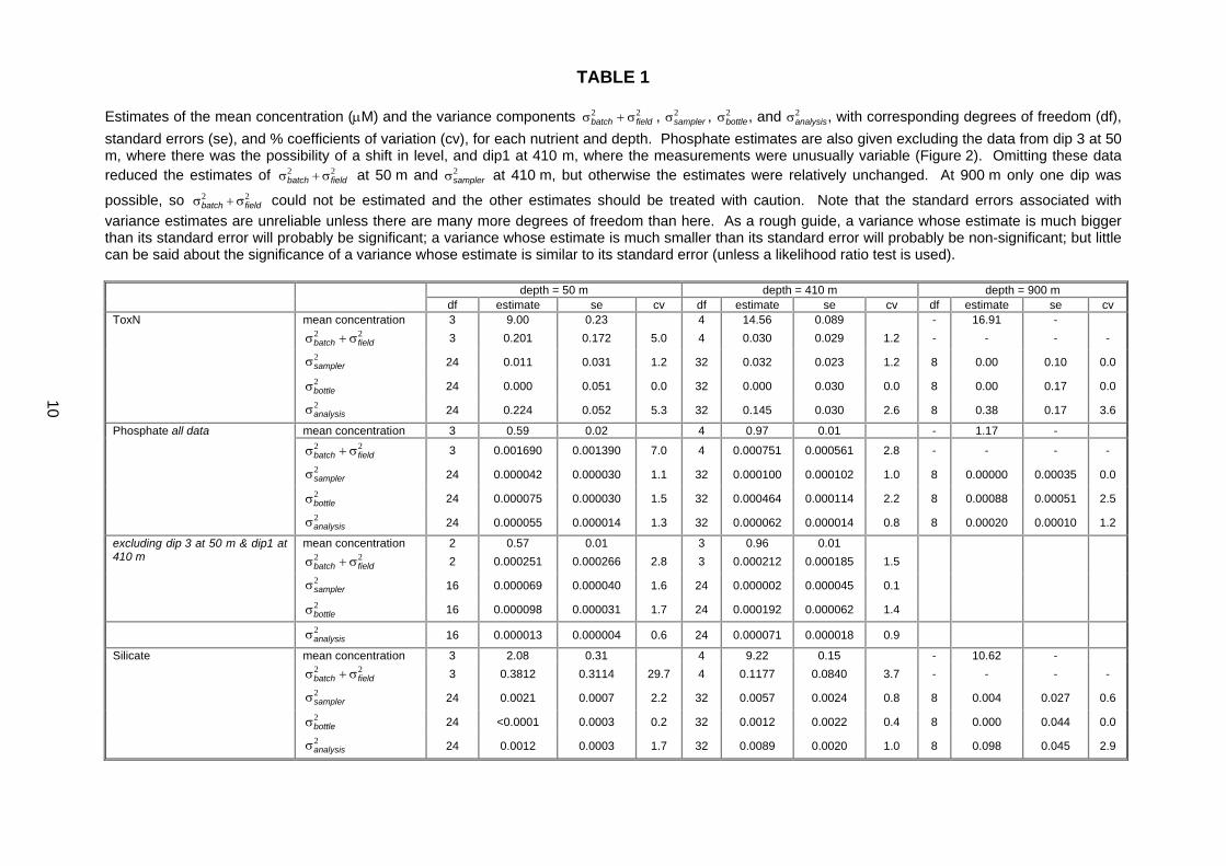
TABLE 1 Estimates of the mean concentration (µM) and the variance components 22
fieldbatch σ+σ , 2samplerσ , 2
bottleσ , and 2analysisσ , with corresponding degrees of freedom (df),
standard errors (se), and % coefficients of variation (cv), for each nutrient and depth. Phosphate estimates are also given excluding the data from dip 3 at 50 m, where there was the possibility of a shift in level, and dip1 at 410 m, where the measurements were unusually variable (Figure 2). Omitting these data reduced the estimates of 22
fieldbatch σ+σ at 50 m and 2samplerσ at 410 m, but otherwise the estimates were relatively unchanged. At 900 m only one dip was
possible, so 22fieldbatch σ+σ could not be estimated and the other estimates should be treated with caution. Note that the standard errors associated with
variance estimates are unreliable unless there are many more degrees of freedom than here. As a rough guide, a variance whose estimate is much bigger than its standard error will probably be significant; a variance whose estimate is much smaller than its standard error will probably be non-significant; but little can be said about the significance of a variance whose estimate is similar to its standard error (unless a likelihood ratio test is used).
depth = 50 m depth = 410 m depth = 900 m df estimate se cv df estimate se cv df estimate se cv
Evaluation of the Sampling and Analytical Technique
11
TABLE 2 Estimates of the mean concentration (µM) and the combined between-analysis and between-batch variance 22
batchanalysis σ+σ , with its corresponding % coefficient of variation (% cv), for certified and laboratory reference materials. A certified reference material was not available for silicate. All laboratory reference materials analysed with each batch were within the Shewhart chart limits and the system suitability checks were acceptable.
certified reference material laboratory reference material 22batchanalysis σ+σ 22
TABLE 3 Estimates of the mean concentration (µM) and the variance components 2
samplerσ , 2bottleσ , 2
batchσ , and 2analysisσ with their corresponding %
coefficients of variation (% cv) for phosphate and silicate, obtained by combining the information from Tables 1 and 2 (see Appendix 1). The table also gives estimates of the overall variance of a nutrient measurement 22222
samplerbottlebatchanalysisnutrient σ+σ+σ+σ=σ and the % contribution of each variance component to the overall variance. Note that estimates for ToxN are not presented, as these would be distorted by the effects of drift and shifts in baseline level; the estimates for phosphate are based on the data from all dips; the estimates at 900 m are based on only one dip, so should be treated with caution; and the laboratory reference material variance estimates in Table 2 were used to estimate 2
batchσ .
depth = 50 m depth = 410 m depth = 900 m
estimate % of total variance % cv estimate % of total
Evaluation of the Sampling and Analytical Technique
13
TABLE 4 Estimates of carryover, with standard errors (se), significance levels (p), and 95% confidence limits. The estimates and 95% confidence limits are expressed in both µM and as percentages of the mean concentrations.
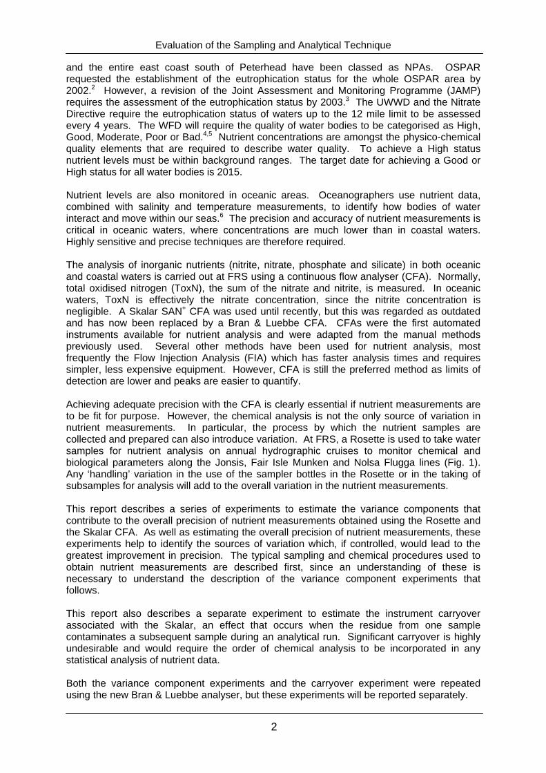
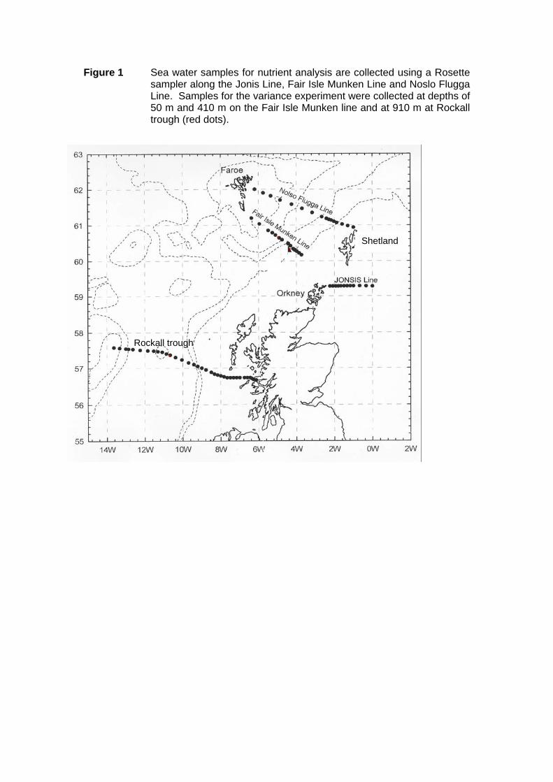
Figure 1 Sea water samples for nutrient analysis are collected using a Rosette sampler along the Jonis Line, Fair Isle Munken Line and Noslo Flugga Line. Samples for the variance experiment were collected at depths of 50 m and 410 m on the Fair Isle Munken line and at 910 m at Rockall trough (red dots).
Rockall
· Shetland
Rockall trough
·
·
Figure 2a Measurements of ToxN concentration (µM) in order of chemical analysis (1-25) for each dip at each depth. The plotting symbol
denotes the sampler number (between 1 and 12), with the absence / presence of a dash denoting a sub-sample bottle from which one / two aliquots was / were taken. There was severe downward drift and shifts in baseline level at all depths.
16.0
16.5
17.0
17.5
18.0
1
96
6
9 51 11
2
2
11
5
1
410
104
11'
2'
4'
6'
5'
1'
10'9'
12'
14.0
14.5
15.0
15.5
1
8 2 3116 4
4
6
2
9
118
5 3
95
4' 5'
7' 6'
9' 2'11'
8'3'
2
6 39
7
12
6 19
11 712 10
1
11
103
1'6' 3' 7'
12'10' 9'
2'11'
3
8 57
7 5
611
44
221212
11
8
6
4'5'
2'12'
10'8'
11'
7'6'
4
5 91 9
14
23
74 2
3
10
7 105
5' 7'
2'
10'
3'11'
9'
4'1'
5
310
16 4
10
4 2 112
83
212
6 8
6'2' 1'
8'4'
10'5'
3' 12'
8.0
8.5
9.0
9.5
10.0
10.5
5 10 15 20 25
1
114 4
116
59
5 1012
109 16
121
11'4'
10'9'
2' 6'12' 1'
5'
5 10 15 20 25
2
11
912
7
45
8
8 912
410
10
57
115'
12'4'
9'
3'7'
8'
10'
11'
5 10 15 20 25
3
104 8 7 8
122 5
121
1
74
52
10
2'
12'8'
7' 1' 4'10'
5'
11'
5 10 15 20 25
4
8610 3
11
6
1083 9 9 1112
7
7 1211'
7' 8'
10' 12'
6'3'
9'1'
depth = 900 m
depth = 410 m
depth = 50 m
order of chemical analysis
ToxN
con
cent
ratio
n (u
M)
Figure 2b Measurements of phosphate concentration (µM) in order of chemical analysis. There was no evidence of severe downward drift
or shifts in baseline level, although closer inspection revealed some possible concerns; for example, the possible shift in level in dip 3 at 50 m. There was large variation between dips at 50 m, indicating large field and / or between-batch variation. The measurements for dip 1 at 410 m were more variable that those for the other dips at this depth.
1.12
1.14
1.16
1.18
1.20
1.22
1
9
6
69
5
1
11
2 2
11
5
1
4
10 10
4
11'2'
4'6'
5'1' 10'
9'
12'
0.90
0.95
1.00
1.05
1.10
18
2
3
11
6 4 46
2
9
11
8
5 3
9
5
4' 5'7' 6'
9'
2'
11'
8'
3'
2
63
97 12
6 19
11 712 10 11110
31' 6'3'
7'
12'10' 9'
2'11'
3
8
5 7 7 5 611
4 42 2
1212
118
64'5' 2'
12' 10'
8'11'7'
6'
4
59 1 9 1 4
2 37 4
2 310
7105
5' 7'2'10'
3'
11' 9'4'
1'
5
3
101
6
4
10
4
2
1
12
83
2
12
6 86'2' 1'8' 4'10' 5'
3' 12'
0.55
0.60
0.65
5 10 15 20 25
1
114 4116
59 5 10
12109 1 6
12111'4' 10'
9' 2'6'
12'1'
5'
5 10 15 20 25
2
119
127
4 5 8 8 912
410
105
7 11
5'
12'4' 9'
3'
7'
8'
10' 11'
5 10 15 20 25
3
104 8 78
122 512
1 1 7 4 5 210
2' 12'
8' 7'
1'
4' 10'5'11'
5 10 15 20 25
4
8 6
10
311
6
10
83
9 911
127
7 1211'
7' 8'10' 12'
6'
3'9' 1'
depth = 900 m
depth = 410 m
depth = 50 m
order of chemical analysis
phos
phat
e co
ncen
tratio
n (u
M)
Figure 2c Measurements of silicate concentration (µM) in order of chemical analysis. There was no evidence of severe downward drift or
shifts in baseline level. There was large variation between dips, particularly at 50 m, indicating large field and / or between-batch variation.
10.2
10.4
10.6
10.8
11.0
1
96
6
9
5
1
11
22
11
5
14
10
10
4
11'2'
4'
6'
5'
1' 10'
9'
12'
8.6
8.8
9.0
9.2
9.4
9.6
9.8
1
8
23
116 44
62
9
118 5 3
9 5
4'5' 7'
6'9' 2' 11'8'
3'
2
6
39
712
61
911
7
12 10
1
11
103
1'
6'3'
7'12' 10' 9'
2'
11'
3
85 7 7
5 611
44
2212
12
118
6
4'
5' 2'12'
10'8'
11'7'
6'
4
59 1
91
42
37
4
2 310
710
5
5'
7'
2'
10' 3' 11'
9'4'
1'
5
3101
6
410
4 2 1
12
83
2
12
68
6'2' 1'
8' 4'
10' 5'
3'
12'
1.5
2.0
2.5
3.0
5 10 15 20 25
1
114 4116 5 9 5 1012 109 1 6 12111' 4'
10'9' 2' 6' 12'1' 5'
5 10 15 20 25
2
119
12 74 5 8 8 9
12
410 10
57
115'
12'4'
9'3'
7'8'
10' 11'
5 10 15 20 25
310
4 8 7 8 122 5121 1 7 4 5 2 102'
12'8' 7' 1' 4' 10'5'11'
5 10 15 20 25
4
8610
3116 108
39 9 11127 7 1211' 7' 8' 10' 12' 6'3'
9' 1'
depth = 900 m
depth = 410 m
depth = 50 m
order of chemical analysis
silic
ate
conc
entra
tion
(uM
)
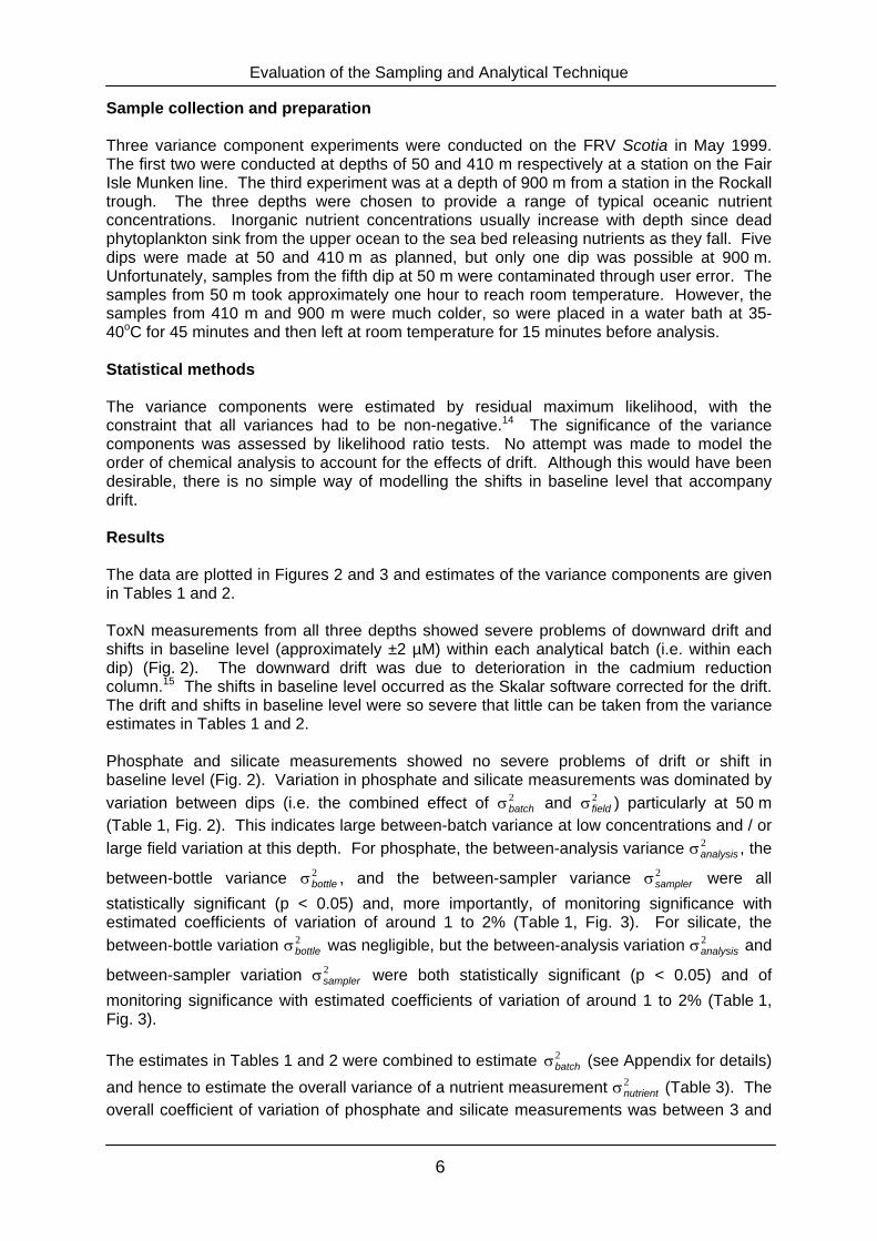
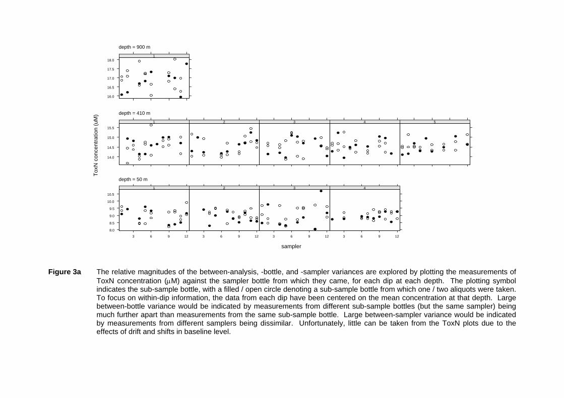
Figure 3a The relative magnitudes of the between-analysis, -bottle, and -sampler variances are explored by plotting the measurements of
ToxN concentration (µM) against the sampler bottle from which they came, for each dip at each depth. The plotting symbol indicates the sub-sample bottle, with a filled / open circle denoting a sub-sample bottle from which one / two aliquots were taken. To focus on within-dip information, the data from each dip have been centered on the mean concentration at that depth. Large between-bottle variance would be indicated by measurements from different sub-sample bottles (but the same sampler) being much further apart than measurements from the same sub-sample bottle. Large between-sampler variance would be indicated by measurements from different samplers being dissimilar. Unfortunately, little can be taken from the ToxN plots due to the effects of drift and shifts in baseline level.
16.0
16.5
17.0
17.5
18.0
1
14.0
14.5
15.0
15.5
1
2
3
4
5
8.0
8.5
9.0
9.5
10.0
10.5
3 6 9 12
1
3 6 9 12
2
3 6 9 12
3
3 6 9 12
4
depth = 900 m
depth = 410 m
depth = 50 m
sampler
ToxN
con
cent
ratio
n (u
M)
1.12
1.14
1.16
1.18
1.20
1.22
1
0.90
0.95
1.00
1.05
1
2
3
4
5
0.56
0.58
0.60
0.62
3 6 9 12
1
3 6 9 12
2
3 6 9 12
3
3 6 9 12
4
depth = 900 m
depth = 410 m
depth = 50 m
sampler
phos
phat
e co
ncen
tratio
n (u
M)
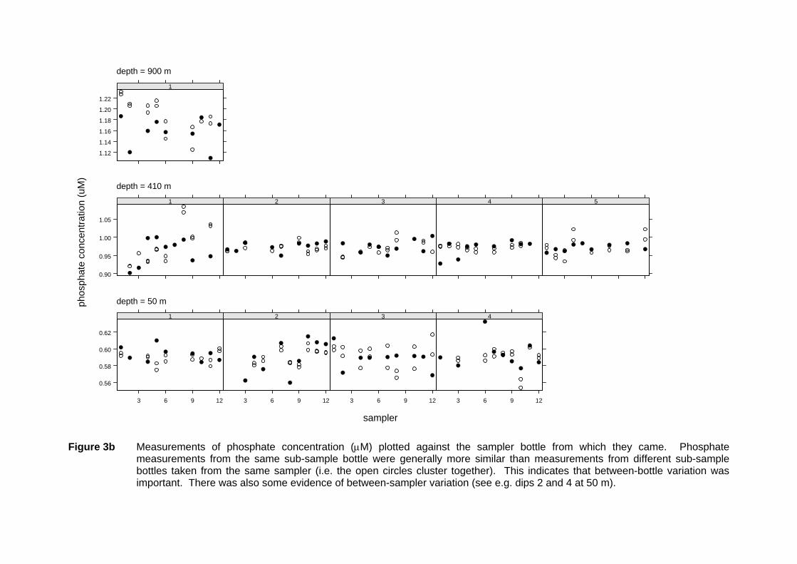
Figure 3b Measurements of phosphate concentration (µM) plotted against the sampler bottle from which they came. Phosphate
measurements from the same sub-sample bottle were generally more similar than measurements from different sub-sample bottles taken from the same sampler (i.e. the open circles cluster together). This indicates that between-bottle variation was important. There was also some evidence of between-sampler variation (see e.g. dips 2 and 4 at 50 m).
10.2
10.4
10.6
10.8
11.0
1
9.0
9.2
9.4
9.6
1
2
3
4
5
2.00
2.05
2.10
2.15
2.20
3 6 9 12
1
3 6 9 12
2
3 6 9 12
3
3 6 9 12
4
depth = 900 m
depth = 410 m
depth = 50 m
sampler
silic
ate
conc
entra
tion
(uM
)
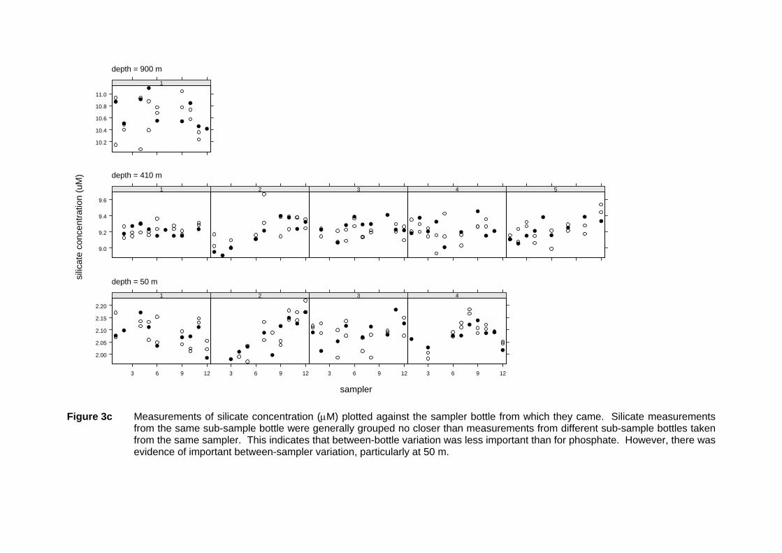
Figure 3c Measurements of silicate concentration (µM) plotted against the sampler bottle from which they came. Silicate measurements
from the same sub-sample bottle were generally grouped no closer than measurements from different sub-sample bottles taken from the same sampler. This indicates that between-bottle variation was less important than for phosphate. However, there was evidence of important between-sampler variation, particularly at 50 m.
ToxN carryover (uM)
-1.5 -1.0 -0.5 0.0 0.5 1.0 1.5
high to low
low to high
phosphate carryover (uM)
-0.010 -0.005 0.0 0.005 0.010
high to low
low to high
silicate carryover (uM)
-0.2 -0.1 0.0 0.1 0.2
high to low
low to high
Figure 4 Box and whisker plots of the differences between 2 successive
measurements of low concentration solution, measuring carryover when moving from high to low concentrations, and the differences between 2 successive measurements of high concentration solution, measuring carryover when from low to high concentration. The filled circles denote the median difference; the open circles show ‘extreme’ differences that were at least 1.5 times the inter-quartile range from the median. The dashed vertical lines indicate zero carryover.
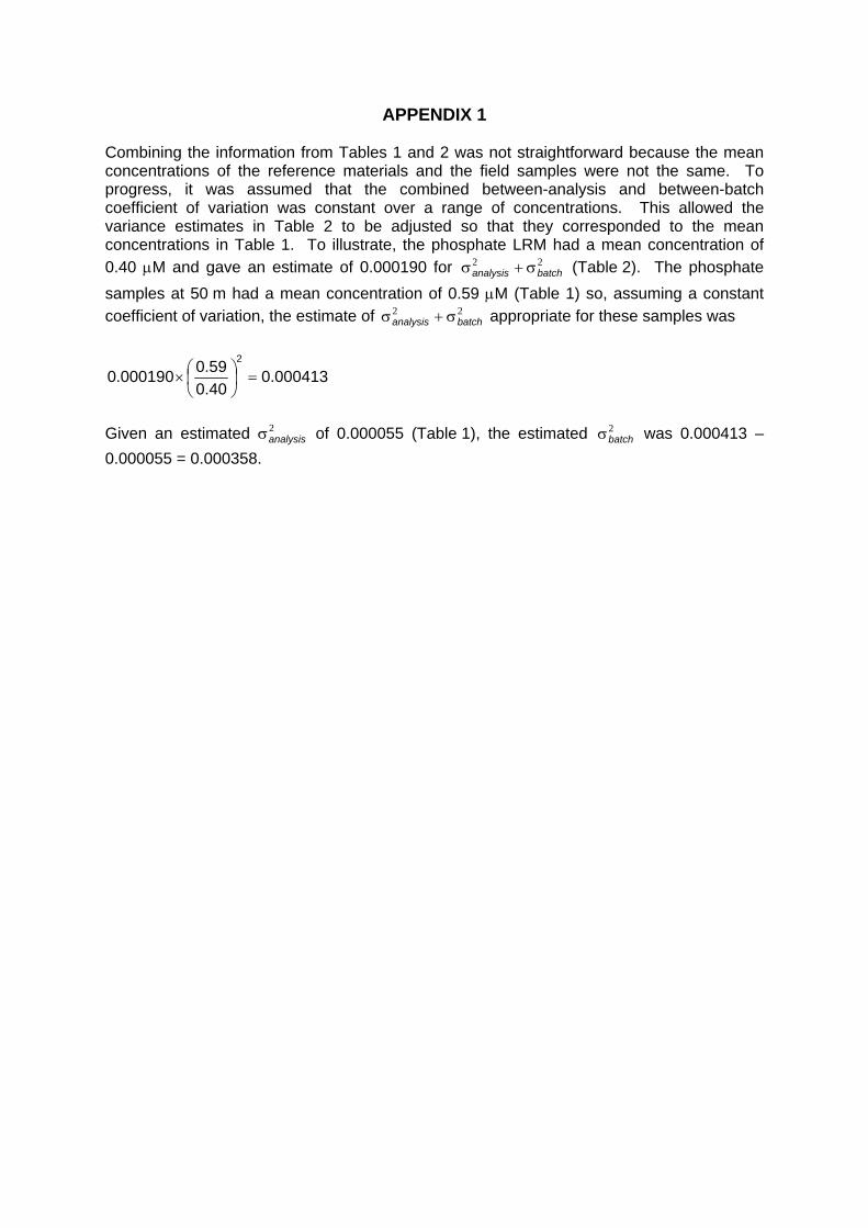
APPENDIX 1 Combining the information from Tables 1 and 2 was not straightforward because the mean concentrations of the reference materials and the field samples were not the same. To progress, it was assumed that the combined between-analysis and between-batch coefficient of variation was constant over a range of concentrations. This allowed the variance estimates in Table 2 to be adjusted so that they corresponded to the mean concentrations in Table 1. To illustrate, the phosphate LRM had a mean concentration of 0.40 µM and gave an estimate of 0.000190 for 22
batchanalysis σ+σ (Table 2). The phosphate samples at 50 m had a mean concentration of 0.59 µM (Table 1) so, assuming a constant coefficient of variation, the estimate of 22
batchanalysis σ+σ appropriate for these samples was
000413.040.059.0000190.0
2
=⎟⎠⎞
⎜⎝⎛×
Given an estimated 2
analysisσ of 0.000055 (Table 1), the estimated 2batchσ was 0.000413 –