Evaluation of Traffic Control Devices, Year 3...Traffic Control Devices, Retroreflective Sign...

Technical Report Documentation Page 1. Report No.

FHWA/TX-12/9-1001-2

2. Government Accession No.

3. Recipient's Catalog No.

4. Title and Subtitle

EVALUATION OF TRAFFIC CONTROL DEVICES, YEAR 3

5. Report Date

Published: March 2012 6. Performing Organization Code

7. Author(s)

Paul J. Carlson, Adam M. Pike, Jeff D. Miles, Brooke R. Ullman, and Darrell W. Borchardt

8. Performing Organization Report No.

Report 9-1001-2

9. Performing Organization Name and Address

Texas Transportation Institute The Texas A&M University System College Station, Texas 77843-3135

10. Work Unit No. (TRAIS)

11. Contract or Grant No.

Project 9-1001 12. Sponsoring Agency Name and Address

Texas Department of Transportation Research and Technology Implementation Office P.O. Box 5080 Austin, Texas 78763-5080

13. Type of Report and Period Covered

Technical Report: September 2010–August 2011 14. Sponsoring Agency Code

15. Supplementary Notes

Project performed in cooperation with the Texas Department of Transportation and the Federal Highway Administration. Project Title: Traffic Control Device Evaluation and Development Program URL: http://tti.tamu.edu/documents/9-1001-2.pdf 16. Abstract

This project was established to provide a means of conducting small-scale research activities on an as-needed basis so that the results could be available within months of starting the specific research. This report summarizes the research activities that were conducted between September 2010 and August 2011. There were five primary activities and five secondary activities. The five primary activities were evaluating nighttime visibility along rural highways with bright signs, continuing the evaluation of lead-free thermoplastic pavement markings, evaluating contrast pavement marking layouts, continuing the evaluation of accelerated pavement marking test decks, and providing district support for hurricane evacuation routing. In addition, the researchers also started to evaluated criteria for setting 80 mph and 85 mph speed limits, evaluated bridge clearance signing, narrowed the focus of a rotational sign sheeting study, provided technical support for the Texas Manual on Uniform Traffic Control Devices (MUTCD), and provided technical support for the Texas Department of Transportation (TxDOT) sign sheeting specification. 17. Key Words

Traffic Control Devices, Retroreflective Sign Sheeting, Hurricane Evacuation, Pavement Marking Retroreflectivity, Contrast Marking

18. Distribution Statement

No restrictions. This document is available to the public through NTIS: National Technical Information Service Alexandria, Virginia 22312 http://www.ntis.gov

19. Security Classif.(of this report)

Unclassified

20. Security Classif.(of this page)

Unclassified 21. No. of Pages

126 22. Price

Form DOT F 1700.7 (8-72) Reproduction of completed page authorized

EVALUATION OF TRAFFIC CONTROL DEVICES, YEAR 3

by

Paul J. Carlson, Ph.D., P.E.

Research Engineer Texas Transportation Institute

Adam M. Pike, P.E.

Assistant Research Engineer Texas Transportation Institute

Jeff D. Miles, P.E.


Brooke R. Ullman, P.E.


Darrell W. Borchardt, P.E. Senior Research Engineer

Texas Transportation Institute

Report 9-1001-2 Project 9-1001

Project Title: Traffic Control Device Evaluation and Development Program

Performed in cooperation with the Texas Department of Transportation

and the Federal Highway Administration

Published: March 2012

TEXAS TRANSPORTATION INSTITUTE The Texas A&M University System College Station, Texas 77843-3135

v

DISCLAIMER

This research was performed in cooperation with the Texas Department of Transportation

(TxDOT) and the Federal Highway Administration (FHWA). The contents of this report reflect

the views of the authors, who are responsible for the facts and the accuracy of the data presented

herein. The contents do not necessarily reflect the official view or policies of the FHWA or

TxDOT. This report does not constitute a standard, specification, or regulation. The engineer in

charge of this project was Paul J. Carlson, P.E. #85402.

vi

ACKNOWLEDGMENTS

This project was conducted in cooperation with TxDOT and FHWA. The authors would

like to thank the project director, Michael Chacon of the TxDOT Traffic Operations Division, for

providing guidance and expertise on this project. Wade Odell of the TxDOT Research and

Technology Implementation Office was the research engineer. The other members of the project

monitoring committee included the following project advisors:

• Ricardo Castaneda, TxDOT San Antonio District.

• John Gianotti, TxDOT San Antonio District.

• Carlos Ibarra, TxDOT Atlanta District.

• Sylvester Onwas, TxDOT Houston District.

• Ismael Soto, TxDOT Corpus Christi District.

• Roy Wright, TxDOT Abilene District.

vii

TABLE OF CONTENTS

Page

LIST OF FIGURES ..................................................................................................................... ix

LIST OF TABLES ....................................................................................................................... xi

CHAPTER 1: OVERVIEW ......................................................................................................... 1

CHAPTER 2: NIGHTTIME VISIBILITY ON RURAL HIGHWAYS WITH BRIGHT SIGNS............................................................................................................................................. 3

OBJECTIVE ............................................................................................................................... 3 Experimental Design ............................................................................................................... 3 Object Detection Task............................................................................................................. 3 Course ..................................................................................................................................... 4 Equipment ............................................................................................................................... 6 Participants .............................................................................................................................. 7 Participant Characteristics ...................................................................................................... 7 Procedure ................................................................................................................................ 7

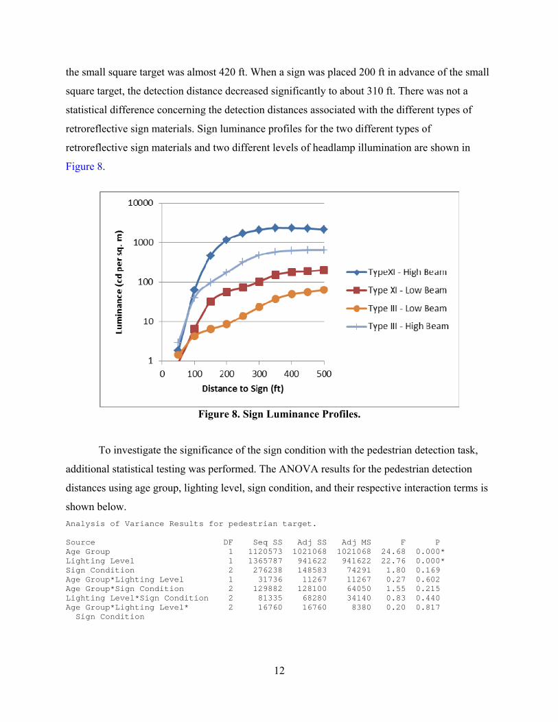
Data Cleaning and Reduction ..................................................................................................... 9 DATA ANALYSIS ..................................................................................................................... 9

Comparison to Previous Work .............................................................................................. 13 Comparison of Results to Design Stopping Sight Distances ................................................ 14

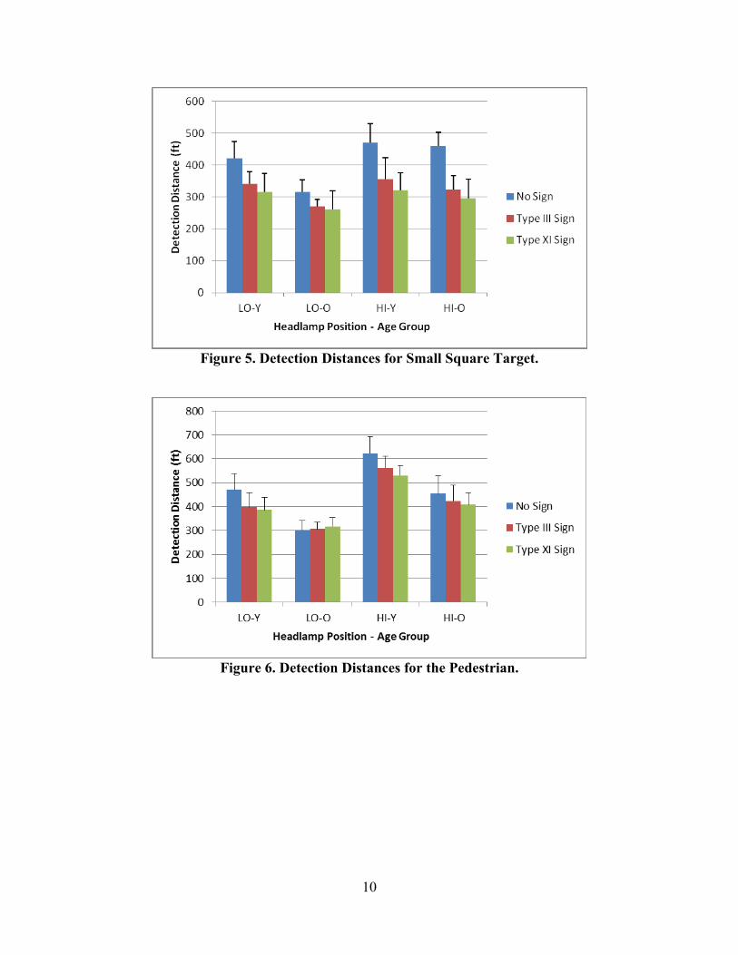
DISCUSSION OF RESULTS................................................................................................... 16 Recommended Follow-Up Research .................................................................................... 18

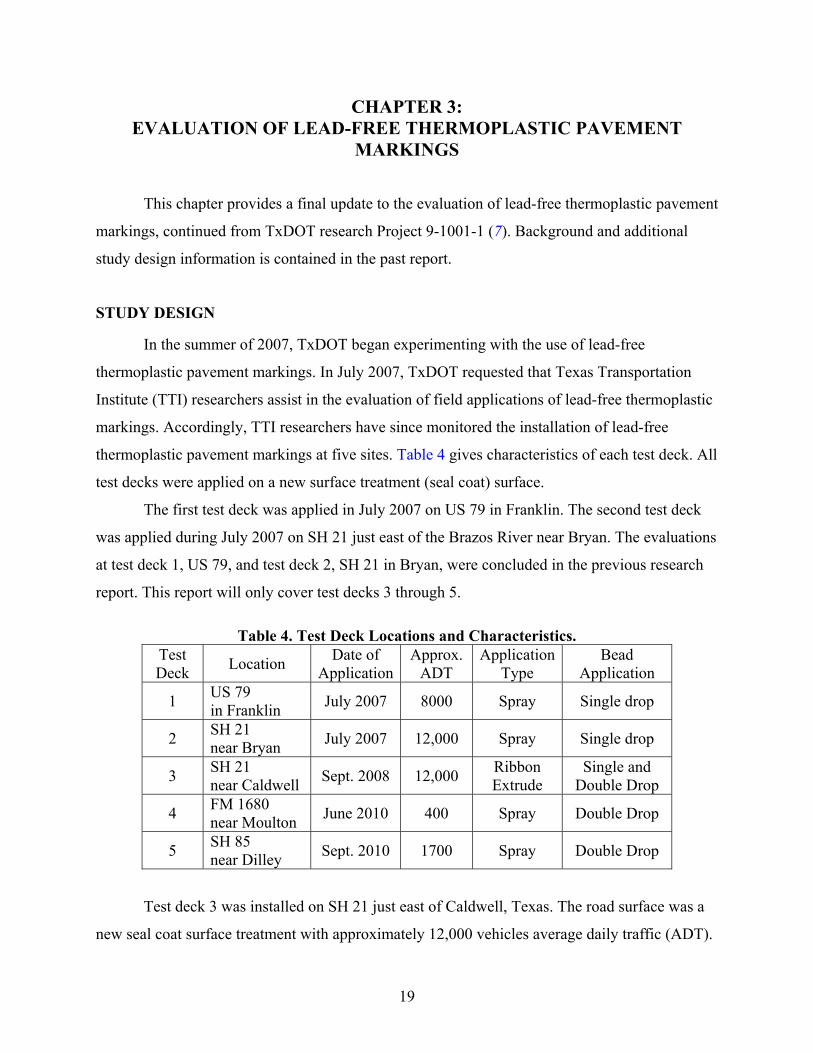
CHAPTER 3: EVALUATION OF LEAD-FREE THERMOPLASTIC PAVEMENT MARKINGS ................................................................................................................................ 19

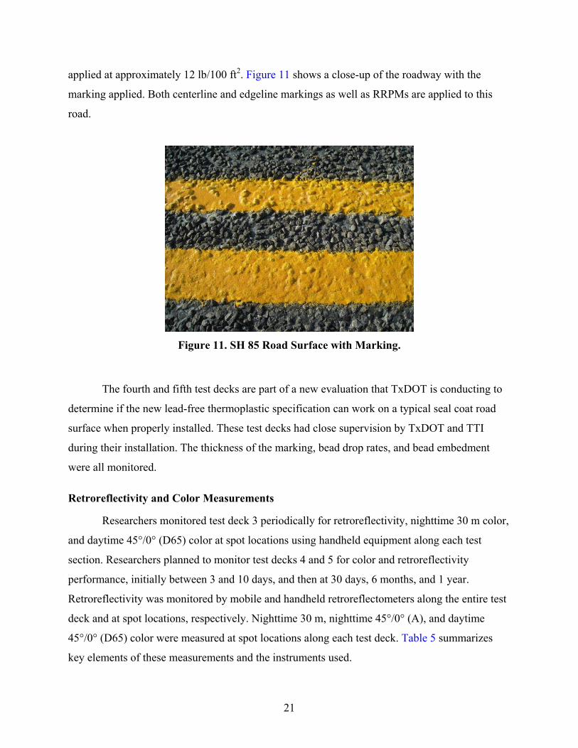
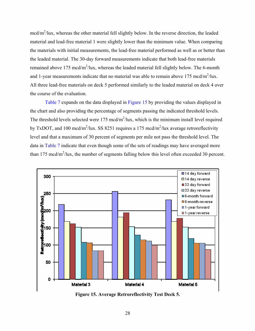
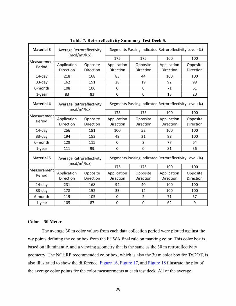
Study Design ............................................................................................................................. 19 Retroreflectivity and Color Measurements ........................................................................... 21

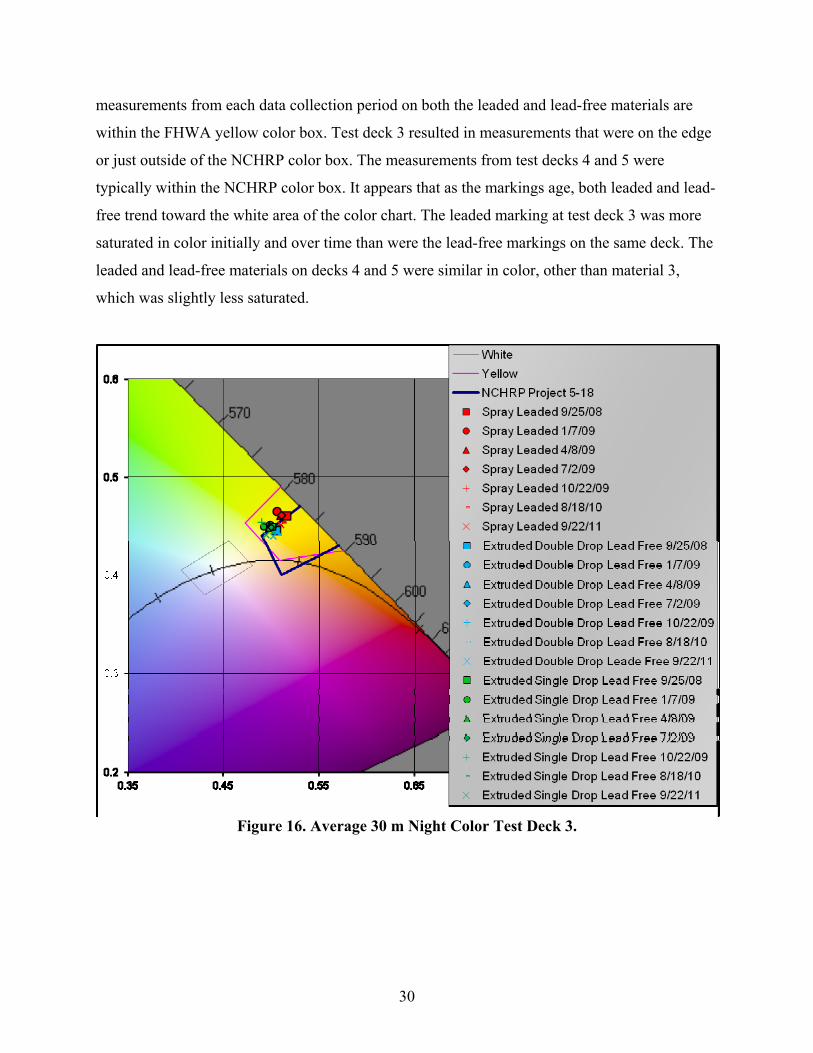
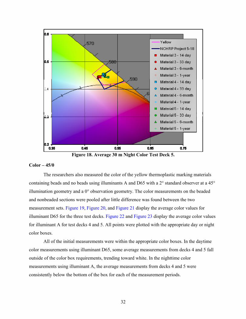
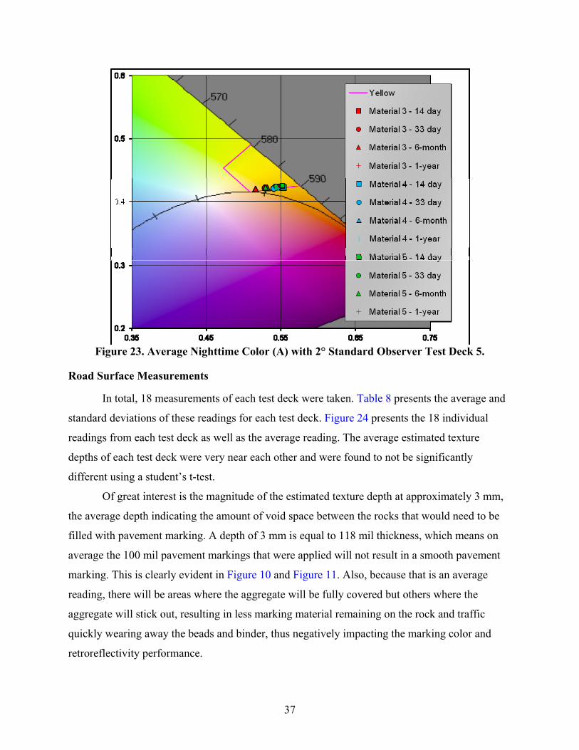
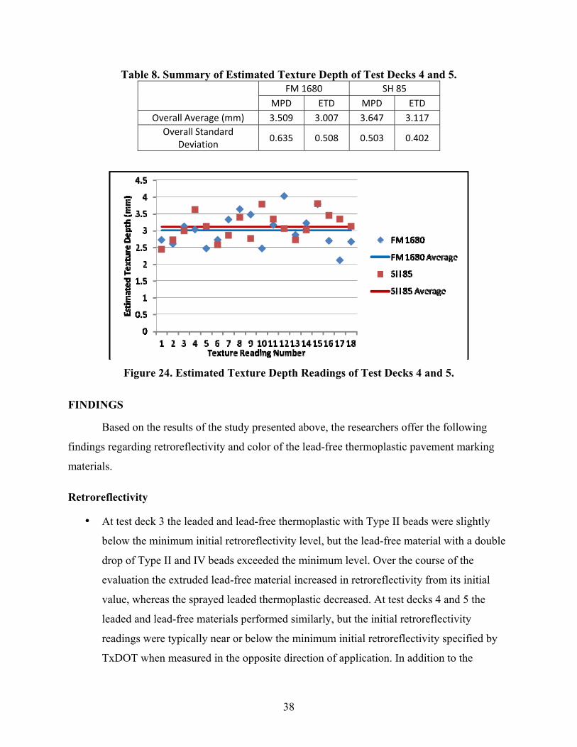
Results ....................................................................................................................................... 23 Retroreflectivity .................................................................................................................... 23 Color – 30 Meter ................................................................................................................... 29 Color – 45/0 .......................................................................................................................... 32 Road Surface Measurements ................................................................................................. 37

Findings..................................................................................................................................... 38 Retroreflectivity .................................................................................................................... 38 30 Meter Nighttime Color ..................................................................................................... 39 45/0 Color ............................................................................................................................. 40

Summary ................................................................................................................................... 40

CHAPTER 4: CONTRAST PAVEMENT MARKING EVALUATION .............................. 43 INTRODUCTION .................................................................................................................... 43 TREATMENTS ........................................................................................................................ 43 STUDY DESIGN...................................................................................................................... 44

Expert Panel Protocol ........................................................................................................... 44

viii

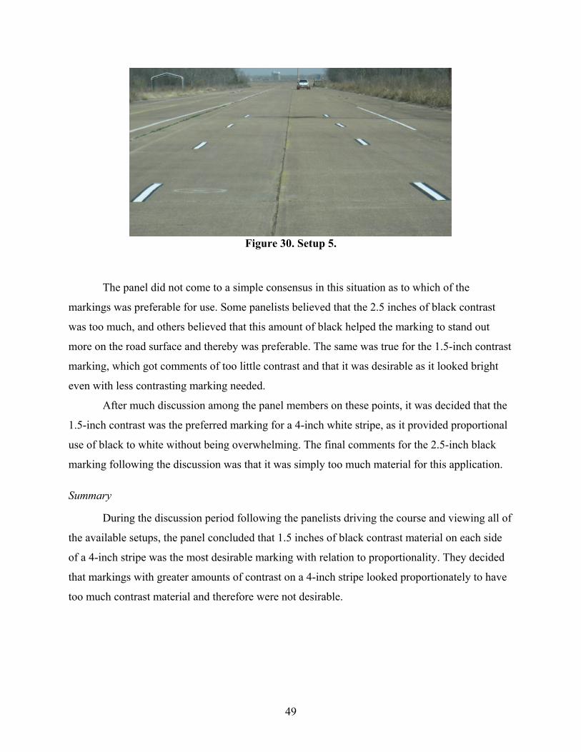
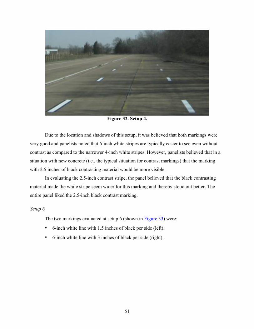
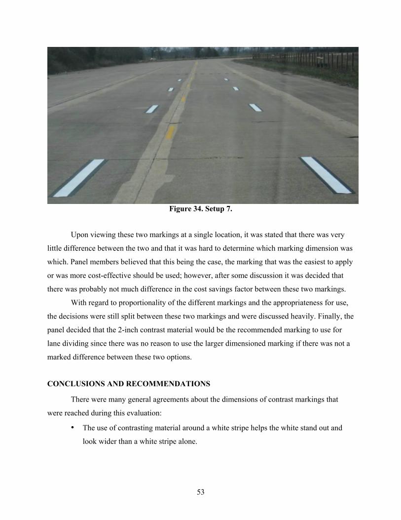
RESULTS ................................................................................................................................. 46 Contrast Markings with Four-Inch White Marking .............................................................. 46 Contrast Markings with Six-Inch White Marking ................................................................ 50

CONCLUSIONS AND RECOMMENDATIONS ................................................................... 53 Recommendations ................................................................................................................. 54

CHAPTER 5: CONTINUED EVALUATION OF PROJECT 0-5548 PAVEMENT MARKING TEST DECKS ........................................................................................................ 55

Background ............................................................................................................................... 55 Research Objectives .................................................................................................................. 55 Test Deck Design ...................................................................................................................... 56

Test Deck Configuration ....................................................................................................... 56 Benefits and Rationales for the Deck Configuration ............................................................ 57

Selection of Test Deck Locations .............................................................................................. 58 Criteria Considered for the Selection of Location ................................................................ 58 Test Deck Locations .............................................................................................................. 59 Products Tested ..................................................................................................................... 59 Test Deck Installation ........................................................................................................... 59 Installation Data by Location ................................................................................................ 60 Data Collection Plan ............................................................................................................. 62

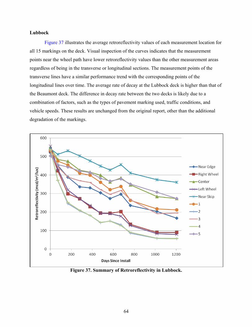
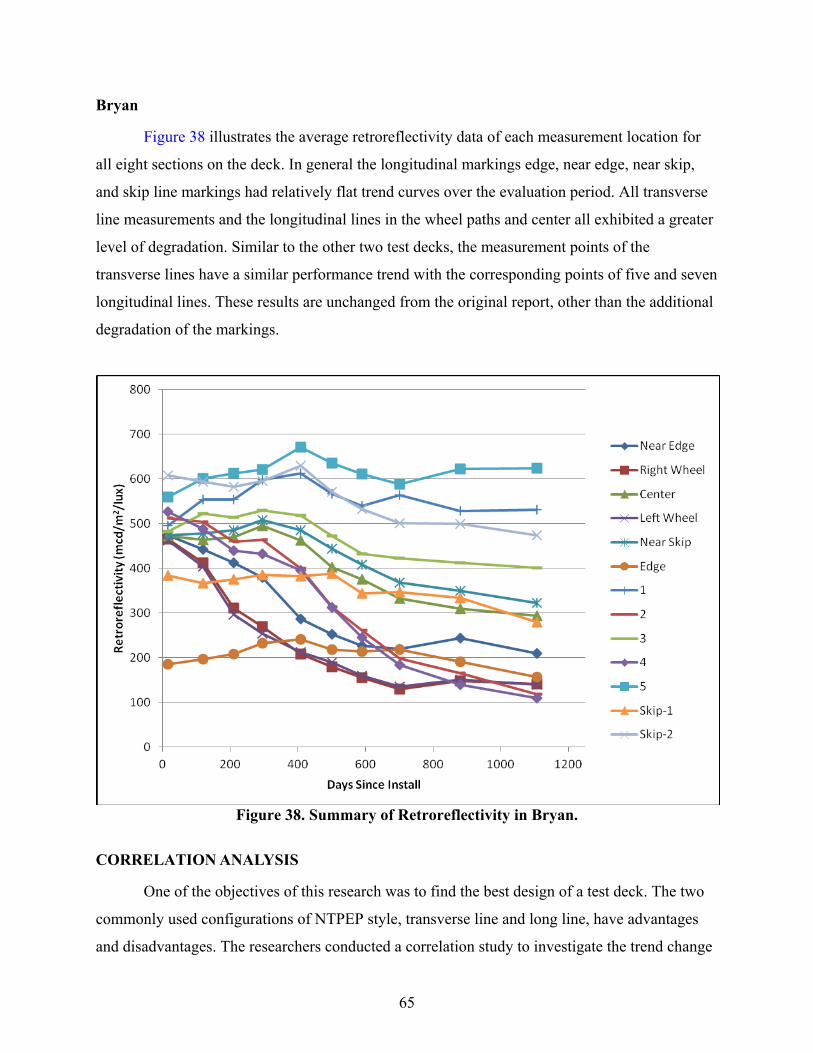
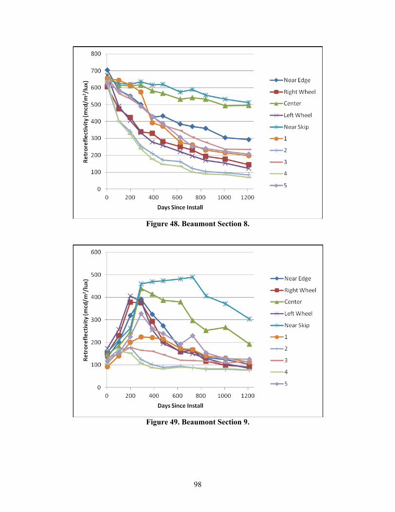
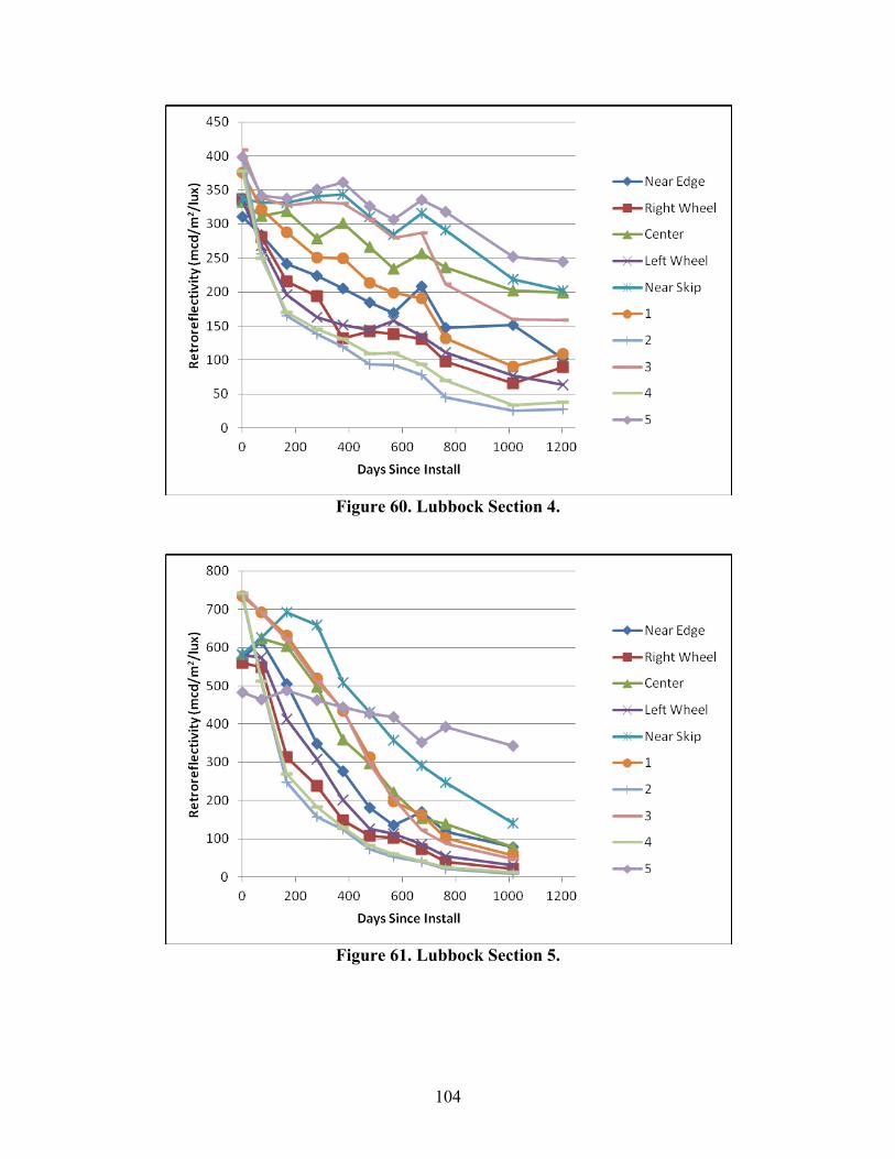
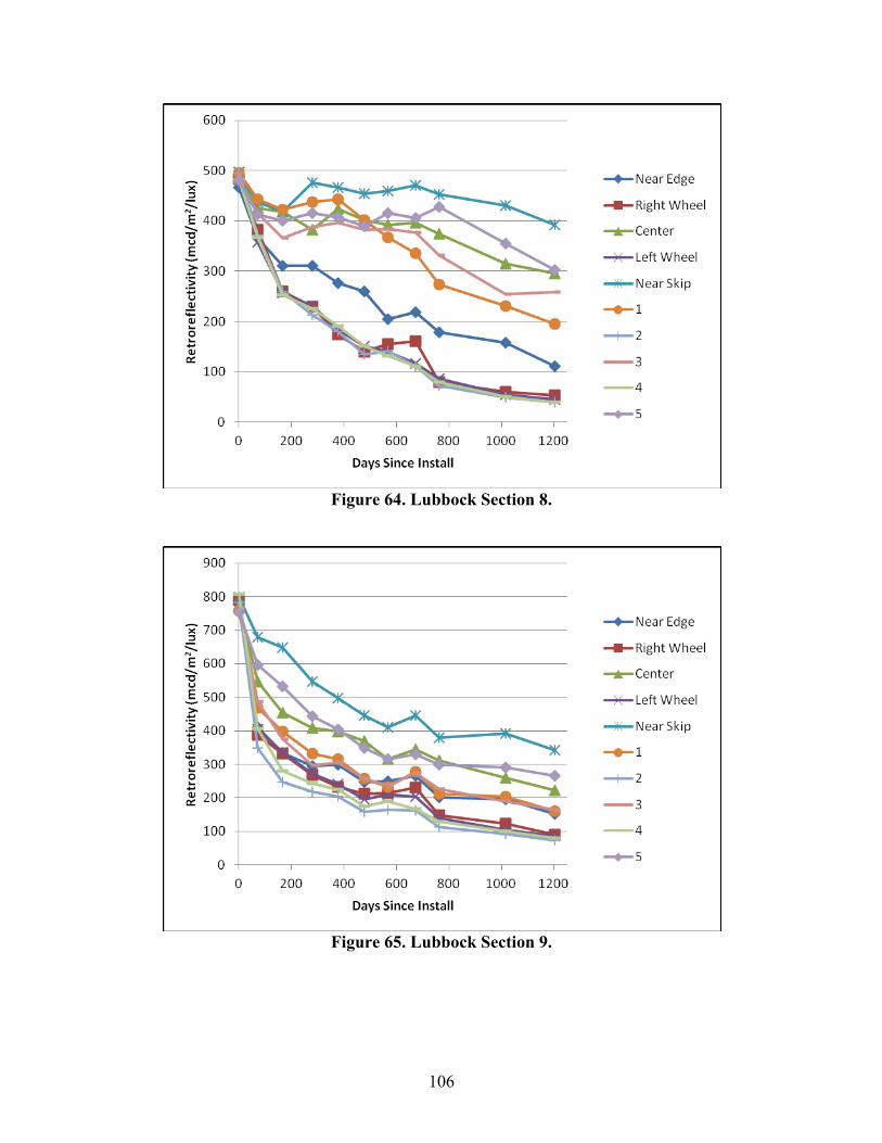
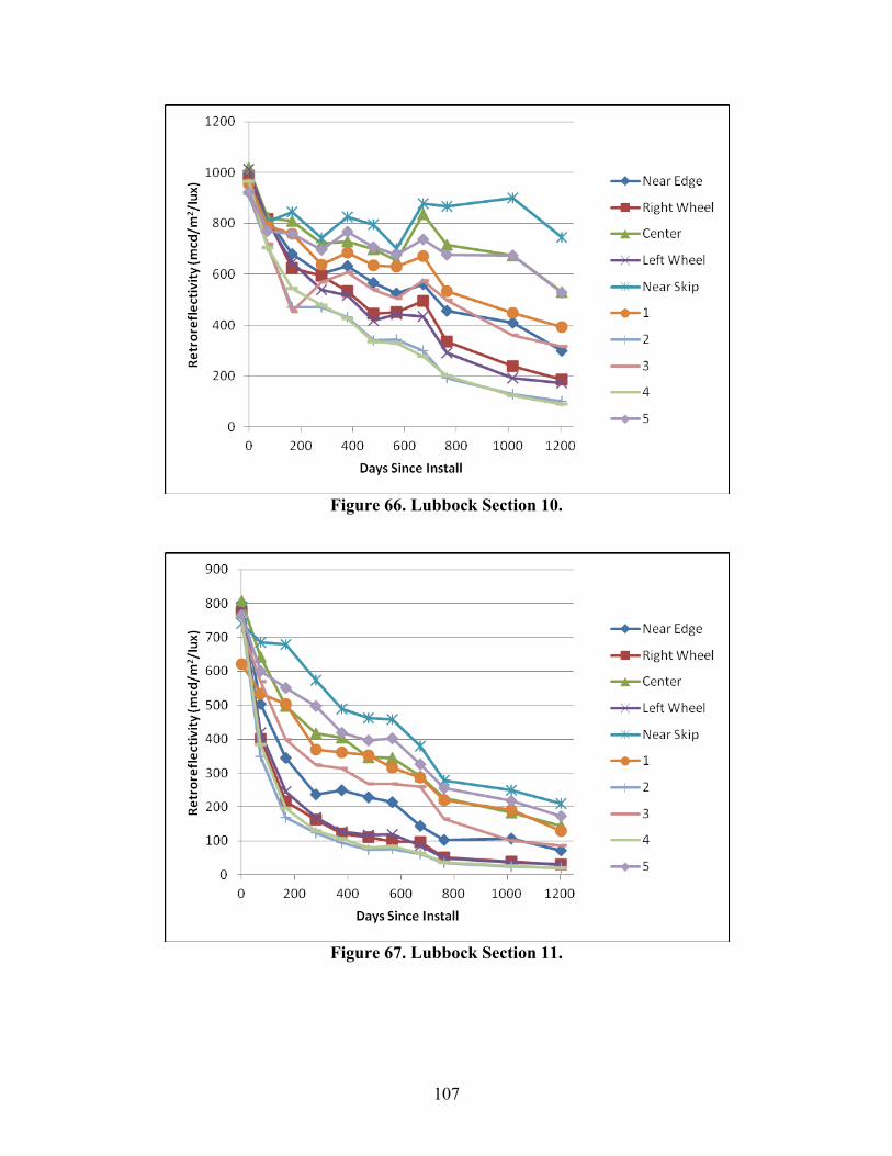
General Performance of Pavement Markings ........................................................................... 62 Beaumont .............................................................................................................................. 63 Lubbock ................................................................................................................................ 64 Bryan ..................................................................................................................................... 65

Correlation Analysis.................................................................................................................. 65 Beaumont .............................................................................................................................. 67 Lubbock ................................................................................................................................ 67 Bryan ..................................................................................................................................... 68

Findings..................................................................................................................................... 68 Recommendations ..................................................................................................................... 70

CHAPTER 6: PROVIDE DISTRICT SUPPORT FOR HURRICANE EVACUATION ROUTING ................................................................................................................................... 73

Development of Hurricane Evacuation Animation Maps for CRP .......................................... 73

CHAPTER 7: ADDITIONAL RESEARCH ACTIVITIES .................................................... 77 85 mph Speed Limit Evaluation ............................................................................................... 77 Bridge Clearance Signing ......................................................................................................... 77 Rotational Sign Sheeting Study ................................................................................................ 82 Technical Support for the Texas MUTCD................................................................................ 84 Technical Support for Texas Sign Sheeting Specification ....................................................... 84

REFERENCES ............................................................................................................................ 95

APPENDIX:................................................................................................................................. 97 Retroreflectivity Degredation Curves for All Pavement Marking Test Decks ......................... 97

ix

LIST OF FIGURES

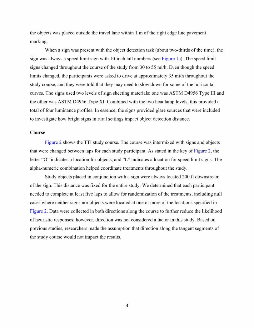
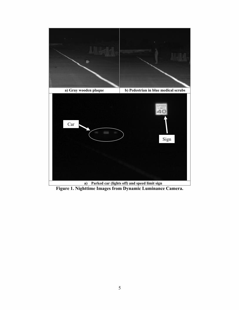
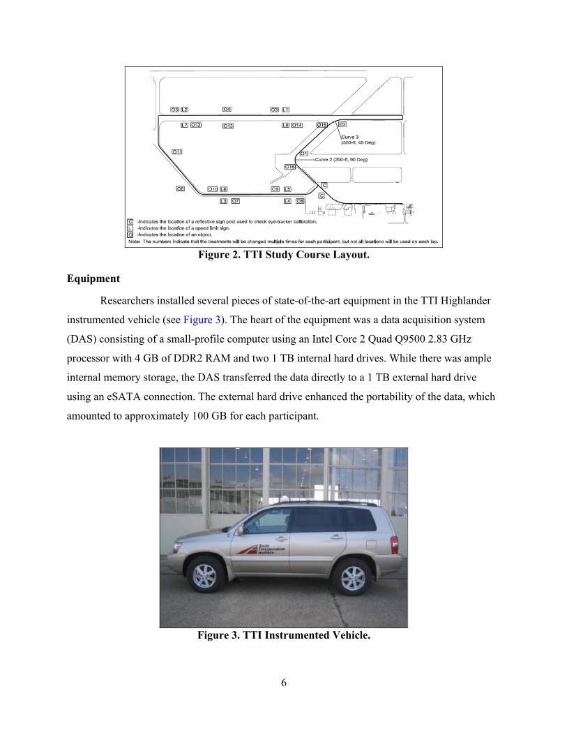
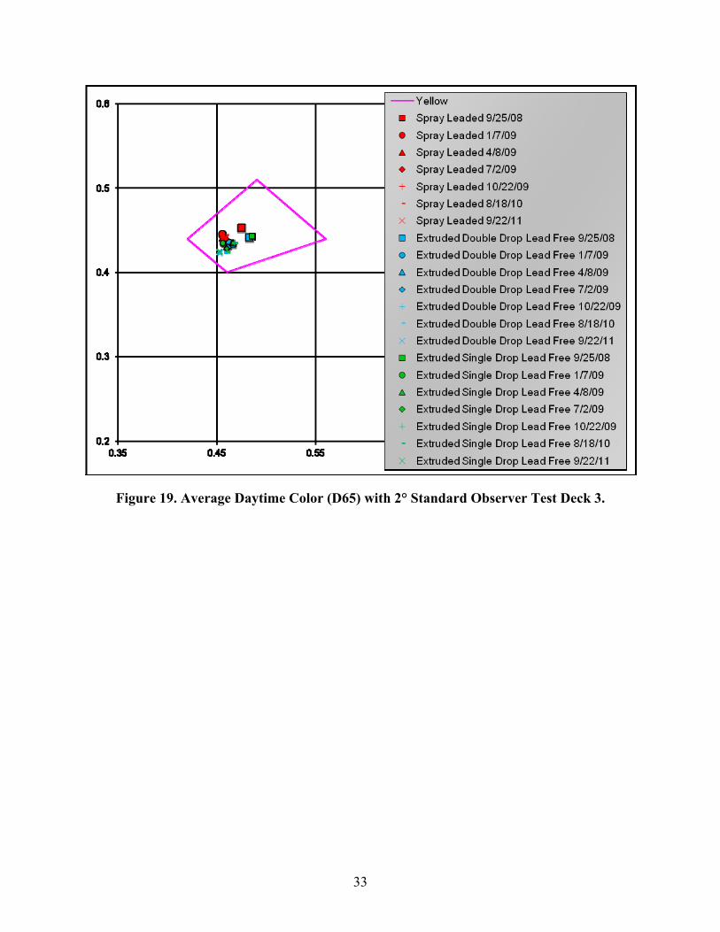
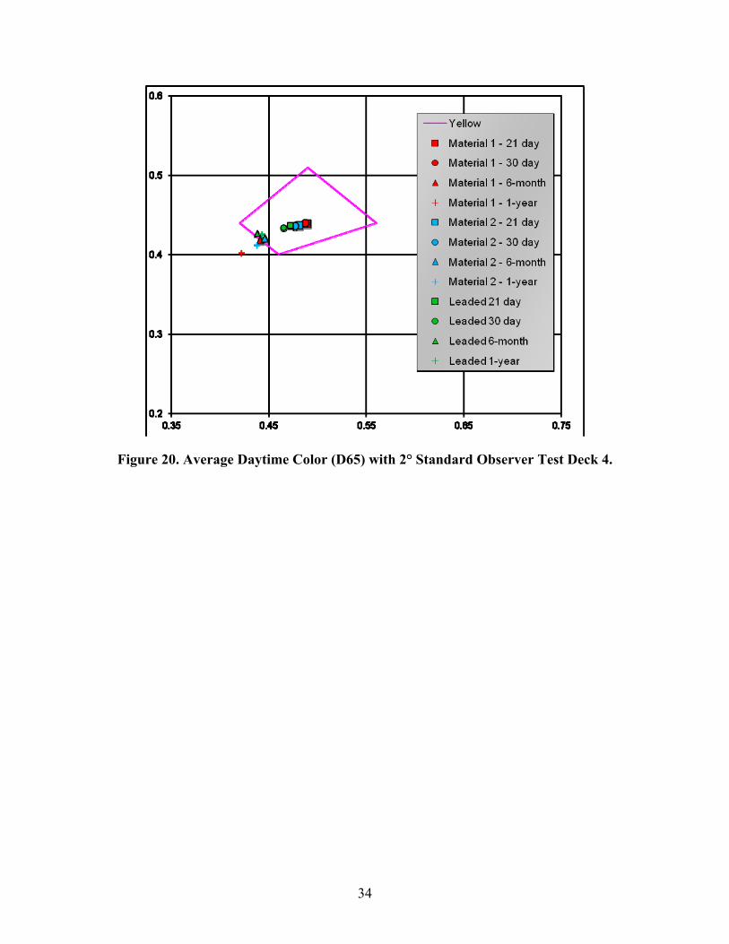
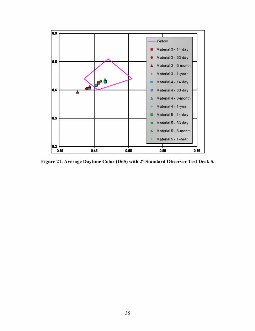
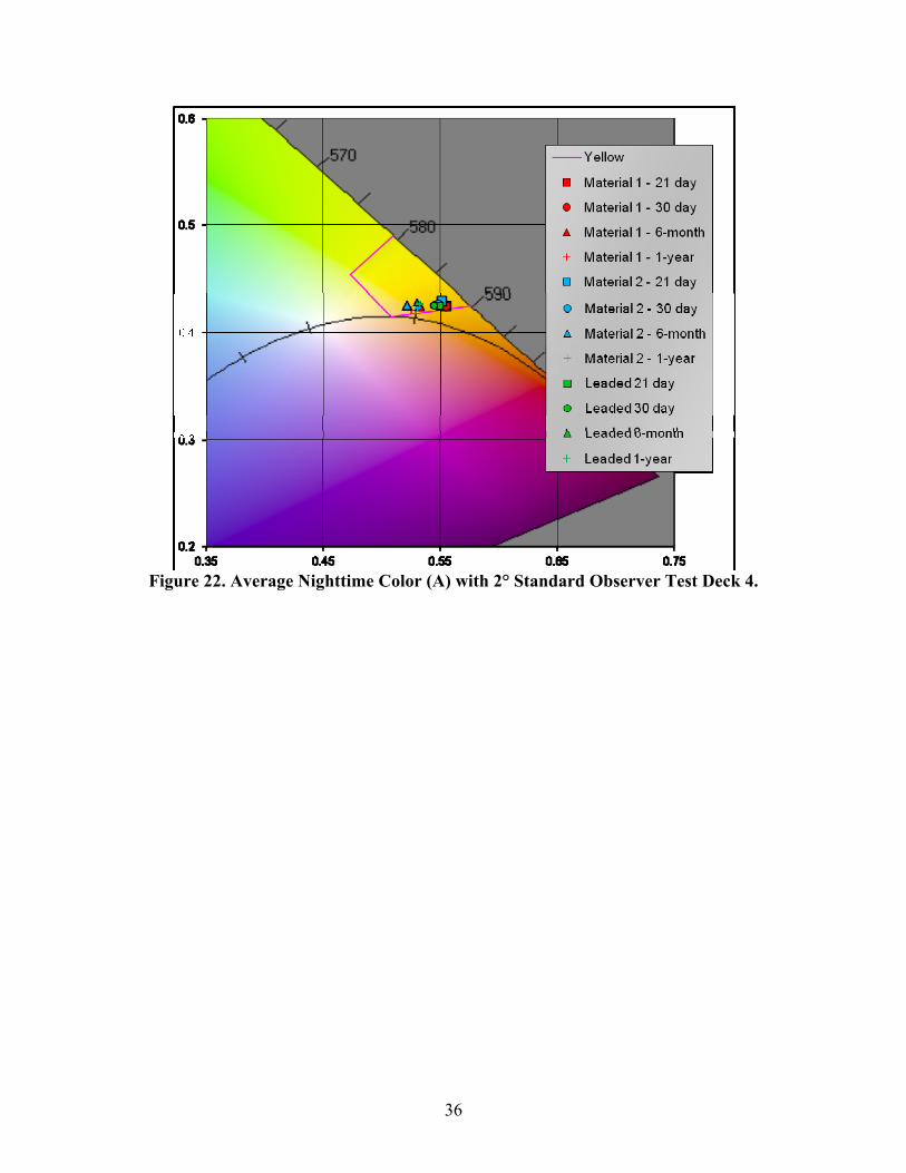
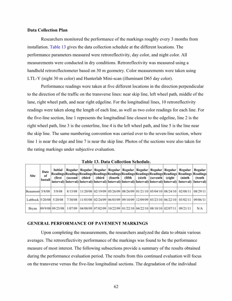
Page Figure 1. Nighttime Images from Dynamic Luminance Camera. .................................................. 5 Figure 2. TTI Study Course Layout. ............................................................................................... 6 Figure 3. TTI Instrumented Vehicle. .............................................................................................. 6 Figure 4. Riverside Campus Test Facility. ...................................................................................... 8 Figure 5. Detection Distances for Small Square Target. .............................................................. 10 Figure 6. Detection Distances for the Pedestrian. ......................................................................... 10 Figure 7. Detection Distances for the Vehicle. ............................................................................. 11 Figure 8. Sign Luminance Profiles. .............................................................................................. 12 Figure 9. Comparison of Detection Distance Data. ...................................................................... 14 Figure 10. FM 1680 Road Surface with Marking ......................................................................... 20 Figure 11. SH 85 Road Surface with Marking ............................................................................. 21 Figure 12. Laser Texture Scanner Taking a Reading. .................................................................. 23 Figure 13. Average Retroreflectivity Test Deck 3. ....................................................................... 24 Figure 14. Average Retroreflectivity Test Deck 4. ....................................................................... 26 Figure 15. Average Retroreflectivity Test Deck 5. ....................................................................... 28 Figure 16. Average 30 Meter Night Color Test Deck 3. .............................................................. 30 Figure 17. Average 30 Meter Night Color Test Deck 4. .............................................................. 31 Figure 18. Average 30 Meter Night Color Test Deck 5. .............................................................. 32 Figure 19. Average Daytime Color (D65) with 2 Degree Standard Observer Test Deck 3. ........ 33 Figure 20. Average Daytime Color (D65) with 2 Degree Standard Observer Test Deck 4. ........ 34 Figure 21. Average Daytime Color (D65) with 2 Degree Standard Observer Test Deck 5. ........ 35 Figure 22. Average Nighttime Color (A) with 2 Degree Standard Observer Test Deck 4. .......... 36 Figure 23. Average Nighttime Color (A) with 2 Degree Standard Observer Test Deck 5. .......... 37 Figure 24. Estimated Texture Depth Readings of Test Deck 4 and 5. .......................................... 38 Figure 25. Contrast Marking Example.......................................................................................... 43 Figure 26. Setup Example. ............................................................................................................ 45 Figure 27. Rating Scales. .............................................................................................................. 45 Figure 28. Setup 1 ......................................................................................................................... 47 Figure 29. Setup 3 ......................................................................................................................... 48 Figure 30. Setup 5 ......................................................................................................................... 49 Figure 31. Setup 2 ......................................................................................................................... 50 Figure 32. Setup 4 ......................................................................................................................... 51 Figure 33. Setup 6 ......................................................................................................................... 52 Figure 34. Setup 7 ......................................................................................................................... 53 Figure 35. Test Deck Configuration. ............................................................................................ 57 Figure 36. Summary of Retroreflectivity in Beaumont. ............................................................... 63 Figure 37. Summary of Retroreflectivity in Lubbock. ................................................................. 64 Figure 38. Summary of Retroreflectivity in Bryan. ...................................................................... 65 Figure 39. Evacuation Routes from Corpus Christi District ......................................................... 75 Figure 40. Initial SH 123 Evacuation Route Overview from PowerPoint .................................... 75 Figure 41. Example of Detailed Routing to Encourage Motorists to Avoid Congestion ............. 76 Figure 42. Example of Inset Map to Provide Turning Directions ................................................ 76

x

Figure 43. Beaumont Section 7. .................................................................................................... 97 Figure 44. Beaumont Section 8. .................................................................................................... 98 Figure 45. Beaumont Section 9. .................................................................................................... 98 Figure 46. Beaumont Section 10. .................................................................................................. 99 Figure 47. Beaumont Section 11. .................................................................................................. 99 Figure 48. Beaumont Section 12. ................................................................................................ 100 Figure 49. Beaumont Section 13. ................................................................................................ 100 Figure 50. Beaumont Section 14. ................................................................................................ 101 Figure 51. Beaumont Section 15. ................................................................................................ 101 Figure 52. Beaumont Section 16. ................................................................................................ 102 Figure 53. Lubbock Section 1. .................................................................................................... 102 Figure 54. Lubbock Section 2. .................................................................................................... 103 Figure 55. Lubbock Section 3. .................................................................................................... 103 Figure 56. Lubbock Section 4. .................................................................................................... 104 Figure 57. Lubbock Section 5. .................................................................................................... 104 Figure 58. Lubbock Section 6. .................................................................................................... 105 Figure 59. Lubbock Section 7. .................................................................................................... 105 Figure 60. Lubbock Section 8. .................................................................................................... 106 Figure 61. Lubbock Section 9. .................................................................................................... 106 Figure 62. Lubbock Section 10. .................................................................................................. 107 Figure 63. Lubbock Section 11. .................................................................................................. 107 Figure 64. Lubbock Section 12. .................................................................................................. 108 Figure 65. Lubbock Section 13. .................................................................................................. 108 Figure 66. Lubbock Section 14. .................................................................................................. 109 Figure 67. Lubbock Section 15. .................................................................................................. 109 Figure 68. Bryan Section 1. ........................................................................................................ 110 Figure 69. Bryan Section 2. ........................................................................................................ 110 Figure 70. Bryan Section 3. ........................................................................................................ 111 Figure 71. Bryan Section 4. ........................................................................................................ 111 Figure 72. Bryan Section 5. ........................................................................................................ 112 Figure 73. Bryan Section 6. ........................................................................................................ 112 Figure 74. Bryan Section 7. ........................................................................................................ 113 Figure 75. Bryan Section 8. ........................................................................................................ 113

xi

LIST OF TABLES

Page Table 1. TTI Experimental Design. ................................................................................................ 3 Table 2. Demographic Data of TTI Participants. ............................................................................ 7 Table 3. Stopping Sight Distances. ............................................................................................... 16 Table 4. Test Deck Locations and Characteristics. ....................................................................... 19 Table 5. Lead-Free Yellow Thermoplastic Pavement Marking Measurements. .......................... 22 Table 6. Retroreflectivity Summary Test Deck 4. ........................................................................ 27 Table 7. Retroreflectivity Summary Test Deck 5. ........................................................................ 29 Table 8. Summary of Estimated Texture Depth of Test Deck 4 and 5. ........................................ 38 Table 9. Study Treatments. ........................................................................................................... 44 Table 10. Beaumont Test Deck Information................................................................................. 60 Table 11. Lubbock Test Deck Information. .................................................................................. 61 Table 12. Bryan Test Deck Information. ...................................................................................... 61 Table 13. Data Collection Schedule. ............................................................................................. 62 Table 14. Correlation between Transverse and Longitudinal Lines. ............................................ 67 Table 15. Correlation between Transverse and Longitudinal Lines in Lubbock. ......................... 67 Table 16. Correlation between Transverse and Longitudinal Lines in Bryan. ............................. 68

1

CHAPTER 1: OVERVIEW

This research project was established as a mechanism for obtaining quick research results

on high-priority traffic control device topics that cannot be programmed in the traditional

research program because of the need for a smaller scope and quicker turnaround time. This

project originally began as TxDOT Project 0-4701, which was active for 5 years (1-5). Upon the

completion of Project 0-4701, a new TxDOT project was started with a similar objective, Project

0-6384, later renumbered Project 9-1001 (6, 7). This report presents the year three activities of

the project.

3

CHAPTER 2: NIGHTTIME VISIBILITY ON RURAL HIGHWAYS WITH BRIGHT

SIGNS

OBJECTIVE

Texas Transportation Institute (TTI) conducted a study to investigate nighttime detection

distances of various objects. The objective of the study was to investigate whether very bright

traffic signs in rural conditions caused limited sight distance beyond the sign. The study included

observations using both low-beam and high-beam headlamp illumination. It also included

detection tasks without a sign present and with signs made of different retroreflective materials.

TTI measured the object detection distance under these different conditions.

Experimental Design

The TTI experimental design investigated the relationship of nighttime visibility and

object detection distance using a 2 × 3 × 2 × 3 experimental design. Table 1 lists the

experiment’s variable conditions.

Table 1. TTI Experimental Design. Variable Levels Participant Age 2: Younger (18–34 years), older (65+ years)

Sign 3: None, ASTM D4956 Type III, and ASTM D4956 Type XI

OEM Headlamps 2: High beam and low beam

Detection Objects 3: Small wood square, static pedestrian, rear of a parked vehicle

OEM = original equipment manufacturer.

Two different age groups participated in the experiment: a younger age group from 18 to

34 years old and an older age group with participants 65 years old and older. The study was

designed to have equal representation of male and female participants, though researchers did not

use gender as a variable in the analysis.

Object Detection Task

For the detection task, researchers used a small gray wooden plaque, a pedestrian in blue

medical scrubs, and the rear of a parked car for the objects (see Figure 1). These objects

replicated previous detection research so that we could compare and contrast the results. Each of

4

the objects was placed outside the travel lane within 1 m of the right edge line pavement

marking.

When a sign was present with the object detection task (about two-thirds of the time), the

sign was always a speed limit sign with 10-inch tall numbers (see Figure 1c). The speed limit

signs changed throughout the course of the study from 30 to 55 mi/h. Even though the speed

limits changed, the participants were asked to drive at approximately 35 mi/h throughout the

study course, and they were told that they may need to slow down for some of the horizontal

curves. The signs used two levels of sign sheeting materials: one was ASTM D4956 Type III and

the other was ASTM D4956 Type XI. Combined with the two headlamp levels, this provided a

total of four luminance profiles. In essence, the signs provided glare sources that were included

to investigate how bright signs in rural settings impact object detection distance.

Course

Figure 2 shows the TTI study course. The course was intermixed with signs and objects

that were changed between laps for each study participant. As stated in the key of Figure 2, the

letter “O” indicates a location for objects, and “L” indicates a location for speed limit signs. The

alpha-numeric combination helped coordinate treatments throughout the study.

Study objects placed in conjunction with a sign were always located 200 ft downstream

of the sign. This distance was fixed for the entire study. We determined that each participant

needed to complete at least five laps to allow for randomization of the treatments, including null

cases where neither signs nor objects were located at one or more of the locations specified in

Figure 2. Data were collected in both directions along the course to further reduce the likelihood

of heuristic responses; however, direction was not considered a factor in this study. Based on

previous studies, researchers made the assumption that direction along the tangent segments of

the study course would not impact the results.

5

a) Gray wooden plaque b) Pedestrian in blue medical scrubs

a) Parked car (lights off) and speed limit sign

Figure 1. Nighttime Images from Dynamic Luminance Camera.

Sign

Car

6

Figure 2. TTI Study Course Layout.

Equipment

Researchers installed several pieces of state-of-the-art equipment in the TTI Highlander

instrumented vehicle (see Figure 3). The heart of the equipment was a data acquisition system

(DAS) consisting of a small-profile computer using an Intel Core 2 Quad Q9500 2.83 GHz

processor with 4 GB of DDR2 RAM and two 1 TB internal hard drives. While there was ample

internal memory storage, the DAS transferred the data directly to a 1 TB external hard drive

using an eSATA connection. The external hard drive enhanced the portability of the data, which

amounted to approximately 100 GB for each participant.

Figure 3. TTI Instrumented Vehicle.

7

Global Positioning System (GPS) data recorded at 5 Hz were used to determine the

detection distances. Researchers developed a separate software package to record GPS data at

5 Hz and export and process those data into X, Y, and Z coordinates with respect to the radius of

the Earth. Each coordinate had an associated time code accurate to within 200 ms, used to select

the GPS location of each object detection reported by each participant. Prior to the start of the

study, the researchers recorded all of the GPS locations of the object and sign locations, and the

resultant distance formula was used during the data reduction to calculate detection distances.

Participants

A total of 31 participants were evaluated in this study with one to two participants studied

each night. All of the participants had 20/40 vision or better and were not color-blind. The

original goal for the distribution of participants was to have six men and six women in age

groups 18–34 and 65 and older, for a total of 24 participants. There were actually five additional

male participants in the age group 18–34. Researchers intended to gather data from at least one

to two more participants within each group to account for any lost data by other participants, but

this did not occur due to scheduling conflicts with the older age group and cancellation or

rescheduling issues that resulted from weather and/or equipment failures.

Participant Characteristics

Table 2 presents the background screening questionnaire that identified participant

demographics and visual acuity information and reflects the average and standard deviation.

Table 2. Demographic Data of TTI Participants. Measure Age Group

18–34 65 +

Mean Age Years (SD) 22.75 (2.5) 73 (4.6)

Mean Visual Acuity (SD) 20.6 (3.9) 22.8 (5.7)

Procedure

Participants drove through a closed-course route at the Texas A&M University Riverside

Campus (see Figure 4) at night. The participants were met at the entrance to the Riverside

8

Campus by TTI staff and then escorted to an office where they completed an informed consent

form, a demographics questionnaire, a Snellen visual-acuity test, and a color-blindness test.

Figure 4. Riverside Campus Test Facility.

Each participant was given some brief instructions about what was required of them.

Provided the participant did not have any reservations about conducting the required tasks, an

experimenter escorted her/him to the instrumented vehicle. Once in the vehicle, each participant

was given an opportunity to familiarize him/herself with the controls of the vehicle and adjust

the vehicle seat to his/her preferences. The participant was instructed to wear a seat belt at all

times during the testing and to alert the researcher to any concerns throughout the study. The

participant was also instructed to stop the vehicle at any point that he/she felt it was necessary.

Researchers designed the on-course study tasks to be similar to typical night driving

activities, such as identifying speed limits for speed adjustments and detecting potential objects

along the roadway that could affect the intended drive path. Prior to starting the study, each

participant was instructed to alert the researcher the instant that he/she detected an object. For the

speed limit signs, the participant was instructed to state the speed limit once it became clear. The

participant was instructed to correct him/herself as soon as possible if he/she incorrectly stated an

observation.

To minimize confusion and response time between the participant and the researcher, the

researcher suggested terms for each object that the participant could consistently use throughout

the data collection: “wood” or “box” for the wooden plaque, “pedestrian” for the pedestrian in

9

blue medical scrubs, “car” for the parked car, and “55” for the sign. Participants used “box” most

often because many of them thought the wooden plaque resembled a gray electrical box like the

ones used in buildings. On the first lap, the participant used either a portion or the entire lap to

become familiar with the procedure.

The in-vehicle researcher guided each participant throughout the driving course. For the

majority of the data collection, the researcher remained silent and allowed the participant to

follow the directions of the pavement markings. Red, retroreflective raised pavement markers

(RRPM) were also placed throughout the course at key turning points and stop locations. Cones

marked an 80-ft radius U-turn. At the end of each lap, the researcher asked the participant to

indicate if she/he had any general or specific comments about the visibility of any of the objects

or signs along the study course during the previous lap.

DATA CLEANING AND REDUCTION

Prior to analyzing the data collected, the research team reduced and cleaned the data.

Data were first transferred from the DAS hard drives and placed on a secure TTI server. Each

data set was then checked for missing data and any errors. Button press corrections and any

anomalies were noted by the in-vehicle experimenter and were also reviewed in conjunction with

the data cleaning process. At this stage, the data were then passed to data specialists for an initial

data cleaning, which included correcting any anomalies noted and verifying button presses.

Ambiguous data were excluded from the overall analysis.

In all, 655 valid detection distances were recorded throughout the project. These

detection distances represent three different objects with and without Speed Limit signs. They

also include observations from both low-beam and high-beam headlamp illumination patterns.

DATA ANALYSIS

The average detection distances for the detection targets are shown in Figure 5 through

Figure 7. The x-axis includes four sets of data. LO represents the vehicle low-beam headlamp

pattern, while HI represents the vehicle high-beam headlamp pattern. Y represents the young

participant age group, and O represents the older participant age group. The T-bars represent one

standard deviation.

10

Figure 5. Detection Distances for Small Square Target.

Figure 6. Detection Distances for the Pedestrian.

11

Figure 7. Detection Distances for the Vehicle.

For all three target types, the results are mostly consistent. In other words, the

participants in the young age group have longer detection distances than those in the old age

group and high-beam vehicle illumination provides longer detection distances than low-beam

vehicle headlamp illumination. The study factor that was not as consistent was the sign condition

(i.e., presence of a sign and what type of retroreflective material was used). In order to study the

data further, statistical testing was implemented using analysis of variance (ANOVA) with

repeated measures. The ANOVA results for small square detection distance using age group,

lighting level, sign condition, and their respective interaction terms is shown below.

Analysis of Variance Results for small square target. Source DF Seq SS Adj SS Adj MS F P Age Group 1 302594 163891 163891 4.52 0.034* Lighting Level 1 229905 200306 200306 5.52 0.019* Sign Condition 2 471076 425187 212594 5.86 0.003* Age Group*Lighting Level 1 11671 395 395 0.01 0.917 Age Group*Sign Condition 2 4016 656 328 0.01 0.991 Lighting Level*Sign Condition 2 24954 39256 19628 0.54 0.583 Age Group*Lighting Level* 2 120761 120761 60380 1.67 0.191 Sign Condition

For the small square target, the main effects of age group, lighting level, and sign

condition are all significant, but no interaction term is significant (factors marked with * are

significant with a p-value < 0.05). With respect to the objective of this study, the sign condition

factor is fundamental. Here sign condition (i.e., no sign, ASTM D4956 Type III sign, or ASTM

D4956 Type XI sign) was significant. The average detection distance with no sign in advance of

12

the small square target was almost 420 ft. When a sign was placed 200 ft in advance of the small

square target, the detection distance decreased significantly to about 310 ft. There was not a

statistical difference concerning the detection distances associated with the different types of

retroreflective sign materials. Sign luminance profiles for the two different types of

retroreflective sign materials and two different levels of headlamp illumination are shown in

Figure 8.

Figure 8. Sign Luminance Profiles.

To investigate the significance of the sign condition with the pedestrian detection task,

additional statistical testing was performed. The ANOVA results for the pedestrian detection

distances using age group, lighting level, sign condition, and their respective interaction terms is

shown below.

Analysis of Variance Results for pedestrian target. Source DF Seq SS Adj SS Adj MS F P Age Group 1 1120573 1021068 1021068 24.68 0.000* Lighting Level 1 1365787 941622 941622 22.76 0.000* Sign Condition 2 276238 148583 74291 1.80 0.169 Age Group*Lighting Level 1 31736 11267 11267 0.27 0.602 Age Group*Sign Condition 2 129882 128100 64050 1.55 0.215 Lighting Level*Sign Condition 2 81335 68280 34140 0.83 0.440 Age Group*Lighting Level* 2 16760 16760 8380 0.20 0.817 Sign Condition

13

Unlike before, the sign condition factor is not significant for the pedestrian. However,

both the age group and lighting level factors were significant (factors marked with * are

significant with a p-value < 0.05).

Statistical testing was also performed with the detection distances from the vehicle

detection task. The ANOVA results for the vehicle detection distances using age group, lighting

level, sign condition, and their respective interaction terms is shown below.

Analysis of Variance Results for vehicle target. Source DF Seq SS Adj SS Adj MS F P Age Group 1 6511576 6406648 6406648 34.12 0.000* Lighting Level 1 2413867 2227208 2227208 11.86 0.001* Sign Condition 2 1759787 1287153 643577 3.43 0.035* Age Group*Lighting Level 1 36474 17460 17460 0.09 0.761 Age Group*Sign Condition 2 251839 242503 121252 0.65 0.525 Lighting Level*Sign Condition 2 53643 50500 25250 0.13 0.874 Age Group*Lighting Level* 2 80987 80987 40493 0.22 0.806 Sign Condition

For the vehicle target, the main effects of age group, lighting level, and sign condition are

all significant, but no interaction term is significant (factors marked with * are significant with a

p-value < 0.05). Interestingly, when the a sign was placed 200 ft in front of the parked vehicle,

the participants were able to detect the vehicle significantly further than without the sign (about

1220 ft without a sign, 1420 ft with the ASTM D4956 Type III sign, and 1350 ft with the ASTM

D4956 Type XI sign).

Comparison to Previous Work

In National Cooperative Highway Research Program (NCHRP) Report 400, similar

research findings are published for nighttime detection distances. With low-beam headlamp

illumination the researchers found that the rear of a vehicle was detected at a range of 550 to

725 ft and then recognized between 725 and 1000 ft. For high-beam illumination, the recognition

distances started at about 1100 ft and the detection distances extended to almost 1800 ft. For

their pedestrian, who was dressed in dark clothing, recognition under low-beam headlamp

illumination was about 100 ft and the detection distance was about 225 ft. Under high-beam

headlamp illumination, the recognition distance was about 300 ft and the detection distance

maxed out at almost 500 ft. A comparison of the detection distance data is shown in Figure 9

(using the data without signs present).

14

Figure 9. Comparison of Detection Distance Data.

The vehicle detection results look quite similar, whereas the pedestrian detection

distances from the report described herein are slightly longer than those found in NCHRP Report

400. There are two likely causes. One is that the description of the pedestrian used for the

NCHRP Report 400 work described dark clothing, while we used blue medical scrubs in this

study, which are not as dark. Another reason could be the evolution of headlamp technologies.

More likely, the longer detection distances found here are based on a combination of the clothing

used in each study and the difference in headlamp flux and patterns.

A key difference of the NCHRP Report 400 work and the work presented in this report is

the evolution of vehicle headlamps. The NCHRP Report 400 work was conducted with a vehicle

with sealed beam headlamps, while the work presented in this report was completed with

modern-day tungsten-halogen headlamps. Another key difference is that we placed objects 1 m

outside of the lane of travel, and the NCHRP Report 400 authors placed objects 1m within the

lane of travel, as measured from the left edgeline of the travel lane. Again, the only description

of the pedestrian was that it was a mannequin dressed in dark clothing.

Comparison of Results to Design Stopping Sight Distances

Sight distance is the length of roadway ahead that is visible to the driver. According to

the TxDOT Design Manual, the available sight distance on a roadway should be sufficiently long

to enable a vehicle traveling at or a near the design speed to stop before reaching a stationary

object in its path. Although greater lengths of visible roadway are desirable, the sight distance at

15

every point along a roadway should be at least that needed for a below-average driver or vehicle

to stop.

Stopping sight distance (SSD) is the sum of two distances: (1) the distance traversed by

the vehicle from the instant the driver sights an object necessitating a stop to the instant the

brakes are applied; and (2) the distance needed to stop the vehicle from the instant brake

application begins. These are referred to as brake reaction distance and braking distance,

respectively.

In computing and measuring SSDs, the height of the driver’s eye is estimated to be 3.5 ft

and the height of the object to be seen by the driver is 2.0 ft, equivalent to the taillight height of a

passenger car. The calculated and design SSDs are shown in Table 3.

Under all conditions studied in this project, the measured detection distance of the parked

vehicle was, on average, greater than the SSD for 80 mph. However, this was the only detection

target with such long detection distances. The small square target and the pedestrian were diffuse

reflectance targets of different sizes and much more difficult to see.

While the pedestrian target was a diffuse reflector, the size was relatively large. The

ANOVA results presented earlier showed that for the pedestrian target the sign condition factor

was not significant. Therefore, the average pedestrian detection under low-beam vehicle

illumination was 363 ft, which would meet the SSD criteria for 45 mph. For high-beam vehicle

illumination, the average pedestrian detection distance was 500 ft, meeting the SSD criteria for a

maximum of 55 mph.

The small square target was also a diffuse reflector but much smaller than the pedestrian

target. The ANOVA results showed that the presence of a sign in front of the small square target

was significant. Therefore, when no sign was present, the small square target had an average

detection distance of 368 ft under low-beam headlamp illumination (adequate for speeds up to 45

mph) and 465 ft under high-beam headlamp illumination (adequate for speeds up to 50 mph).

With a sign located 200 ft before the small square target, the average detection distance was only

297 ft under low-beam headlamp illumination (adequate for speeds up to 35 mph) and 314 ft

under high-beam headlamp illumination (adequate for speeds up to 40 mph).

16

Table 3. Stopping Sight Distances. Design

Speed

(mi/h)

Brake reaction

distance

(ft)

Braking distance on

level

(ft)

Calculated SSD

(ft)

Design SSD

(ft)

15 55.1 21.6 76.7 80

20 73.5 38.4 111.9 115

25 91.9 60.0 151.9 155

30 110.3 86.4 196.7 200

35 128.6 117.6 246.2 250

40 147.0 153.6 300.6 305

45 165.4 194.4 359.8 360

50 183.8 240.0 423.8 425

55 202.1 290.3 492.4 495

60 220.5 345.5 566.0 570

65 238.9 405.5 644.4 645

70 257.3 470.3 727.6 730

75 275.6 539.9 815.5 820

80 294.0 614.3 908.3 910

DISCUSSION OF RESULTS

To summarize, nighttime detection distances of three different objects (a small square

target, a pedestrian, and a parked vehicle) were obtained under two different vehicle headlamp

illumination patterns. The study also included a sign condition factor made up of three levels: no

sign present, a white speed limit sign made with ASTM D4956 Type III retroreflective sheeting

material, and a white speed limit sign made with ASTM D4956 Type XI retroreflective sheeting

material. When the signs were present, they were always 200 ft in advance of the objects. The

sign condition factor was added to study the impact of sight distance along dark rural roads when

bright signs are present.

Of the three objects, the parked vehicle was most easily detected, regardless of the

headlamp illumination setting or presence of an upstream sign. The average detection distances

17

were beyond the 80 mph SSD criteria. The parked vehicle was the only detection target with

retroreflective elements. The other detection targets were diffuse reflective and produced much

more interesting results.

Two sizes of diffuse reflective targets were used: a small square target (measuring 7 by

7 inch) and a stationary pedestrian dressed in blue medical scrubs. The different sizes of these

detection targets appear to have been a major factor in the results.

For the larger target, the stationary pedestrian, the detection distances were not

statistically impacted by the presence or type of upstream sign (p-value = 0.169). However, for

the smaller and more difficult to see target, the small square, the detection distances were

statistically significantly lower when the upstream sign was present compared to when it was not

present. Even though the detection distances were slightly longer under high-beam vehicle

illumination, this difference between no sign and sign present was doubled under high-beam

vehicle illumination compared to low-beam vehicle illumination (70 ft reduction versus 141 ft

reduction). This can create an unsafe driving environment at night because of violated driver

expectancy of longer visibility under high-beam illumination conditions. Under these conditions,

the detection distances were only adequate for speeds up to 40 mph (compared to 50 mph

without a sign present).

The presence of bright signs along a rural highway appears to have increasing impact as

the detection task becomes harder. For the easy-to-see parked vehicle, the presence or brightness

of the sign is not of concern since the detection distances were beyond 80 mph SSD criteria. For

the harder-to-see pedestrian, the presence or brightness of the sign has no statistically significant

impact. However, for the hardest-to-see small square target, the presence of the sign statistically

significantly lowered the detection distance. This impact was doubled under high-beam vehicle

headlamp illumination.

The findings imply that nighttime rural highway drivers do not have the visual

capabilities or illumination levels needed to detect small- to medium-sized objects beyond

minimum stopping sight distances for 55 mph under best-scenario conditions or 35 mph under

worst-case-scenario conditions. Of course, detection does not necessarily require stopping. A

driver must be able to recognize an object as a hazard in time to safely stop or maneuver around

it. Given the detection distances in this study, drivers would have between 2.6 (310 ft detection

18

at 80 mi/h) and 5.2 (420 ft detection at 55 mi/h) seconds to react to the small low-contrast objects

along highways in Texas, depending on the speed limit.

The average detection distance findings were compared to SSD criteria. The results are

somewhat alarming knowing that TxDOT highways will soon be posted with a speed limit of

75 mph that is applicable to both day and nighttime conditions. The results would have even

worse if the 15th percentile detection distances were used rather than the average detection

distances. It is reasonable to use the 15th percentile levels to accommodate the majority of the

drivers.

Recommended Follow-Up Research

This study was conducted as an investigative study into the impacts on object detection

distances of bright signs on rural highways. A goal of the study was to determine if there is

justification for setting maximum levels of sign retroreflectivity for rural highways. It has been

reported by several transportation officials that the newer prismatic signs along dark rural

stretches of highway appear too bright. While anecdotal comments have also been reported on

previous research studies such as TxDOT Project 0-5235, no research study has focused on the

question of whether under some conditions traffic signs can be too bright.

A follow-up study is recommended that will include different objects (a deer rather than

the parked vehicle) and various distances between the objects and the sign. An inspection of the

luminance curves shown in Figure 8 and the average detection distances reveals that objects

closer to the sign would be even harder to detect than those placed 200 ft downstream of the

sign. In addition, the research team proposes that follow-up research consider different pavement

types. This study was conducted on concrete pavement, which provides different contrast ratios

than asphalt or seal-coat pavements, which are much more common in Texas.

19

CHAPTER 3: EVALUATION OF LEAD-FREE THERMOPLASTIC PAVEMENT

MARKINGS

This chapter provides a final update to the evaluation of lead-free thermoplastic pavement

markings, continued from TxDOT research Project 9-1001-1 (7). Background and additional

study design information is contained in the past report.

STUDY DESIGN

In the summer of 2007, TxDOT began experimenting with the use of lead-free

thermoplastic pavement markings. In July 2007, TxDOT requested that Texas Transportation

Institute (TTI) researchers assist in the evaluation of field applications of lead-free thermoplastic

markings. Accordingly, TTI researchers have since monitored the installation of lead-free

thermoplastic pavement markings at five sites. Table 4 gives characteristics of each test deck. All

test decks were applied on a new surface treatment (seal coat) surface.

The first test deck was applied in July 2007 on US 79 in Franklin. The second test deck

was applied during July 2007 on SH 21 just east of the Brazos River near Bryan. The evaluations

at test deck 1, US 79, and test deck 2, SH 21 in Bryan, were concluded in the previous research

report. This report will only cover test decks 3 through 5.

Table 4. Test Deck Locations and Characteristics. Test Deck

Location Date of

ApplicationApprox.

ADT Application

Type Bead

Application

1 US 79 in Franklin

July 2007 8000 Spray Single drop

2 SH 21 near Bryan

July 2007 12,000 Spray Single drop

3 SH 21 near Caldwell

Sept. 2008 12,000 Ribbon Extrude

Single and Double Drop

4 FM 1680 near Moulton

June 2010 400 Spray Double Drop

5 SH 85 near Dilley

Sept. 2010 1700 Spray Double Drop

Test deck 3 was installed on SH 21 just east of Caldwell, Texas. The road surface was a

new seal coat surface treatment with approximately 12,000 vehicles average daily traffic (ADT).

20

Contractors applied standard spray-applied thermoplastic with Type II beads along the road as

part of the contract to resurface the road. A portion of road was left without edgeline markings so

that the test markings could be installed. The test marking installed was a lead-free thermoplastic

applied by ribbon extrusion. Two different sections were applied: one section had a double drop

of Type II and Type IV beads, and the second section had only Type II beads for comparison to

the standard marking. This section of roadway is a grass median-divided four-lane highway with

both yellow and white edge markings and white lane line markings supplemented with RRPMs.

Test deck 4 was installed in June 2010 on FM 1680 near Moulton, Texas. The road

surface was a new seal coat surface treatment with approximately 400 ADT. This section

compared two lead-free materials to an adjacent leaded material. Each of the three materials was

spray applied for approximately 4 miles. The markings were applied at approximately 100 mil

thick and had a double drop of Type II and III beads each applied at approximately 12 lb/100 ft2.

Figure 10 shows a typical section of the roadway with the marking applied. Only centerline

markings and RRPMs are applied to this road.

Figure 10. FM 1680 Road Surface with Marking.

Test deck 5 was installed in September 2010 on SH 85 near Dilley, Texas. The road

surface was a new seal coat surface treatment with approximately 1700 ADT. Three different

marking materials were applied; each test section is approximately 4 miles long. The markings

were applied at approximately 100 mil thick and had a double drop of Type II and III beads, each

21

applied at approximately 12 lb/100 ft2. Figure 11 shows a close-up of the roadway with the

marking applied. Both centerline and edgeline markings as well as RRPMs are applied to this

road.

Figure 11. SH 85 Road Surface with Marking.

The fourth and fifth test decks are part of a new evaluation that TxDOT is conducting to

determine if the new lead-free thermoplastic specification can work on a typical seal coat road

surface when properly installed. These test decks had close supervision by TxDOT and TTI

during their installation. The thickness of the marking, bead drop rates, and bead embedment

were all monitored.

Retroreflectivity and Color Measurements

Researchers monitored test deck 3 periodically for retroreflectivity, nighttime 30 m color,

and daytime 45°/0° (D65) color at spot locations using handheld equipment along each test

section. Researchers planned to monitor test decks 4 and 5 for color and retroreflectivity

performance, initially between 3 and 10 days, and then at 30 days, 6 months, and 1 year.

Retroreflectivity was monitored by mobile and handheld retroreflectometers along the entire test

deck and at spot locations, respectively. Nighttime 30 m, nighttime 45°/0° (A), and daytime

45°/0° (D65) color were measured at spot locations along each test deck. Table 5 summarizes

key elements of these measurements and the instruments used.

22

The measurements were compared to minimum retroreflectivity levels and color boxes

where appropriate. The minimum initial retroreflectivity level of 175 mcd/m2/lux for yellow

pavement markings is contained in Special Specification (SS) 8251, Reflectorized Pavement

Markings with Retroreflective Requirements (8). Several different chromaticity coordinate boxes

exist for pavement markings. The TxDOT chromaticity coordinate boxes for yellow markings

are contained in DMS-8220, Hot Applied Thermoplastic (9). The July 31, 2002, Final Rule by

the Federal Highway Administration (FHWA), also established daytime (45/0) 2° standard

observer and nighttime (30 m) chromaticity coordinate boxes for traffic materials (10).

Table 5. Lead-Free Yellow Thermoplastic Pavement Marking Measurements.

Attribute Measurement Geometry Instrument Description

Retro-reflectivity

30 m LTL 2000SY A measure of the amount of light retroreflected to the driver from the pavement marking.

30 m Laserlux Mobile readings of retroreflectivity.

Nighttime Color

30 m LTL 2000SY A measure of the nighttime color of the pavement marking as viewed by the driver.

45/0 Hunterlab MiniScan

XE Plus

A measure of color using Illuminant A and the standard color measurement geometry. The 2° standard observer was used for all measurements.

Daytime Color

45/0 Hunterlab MiniScan

XE Plus

A measure of color using Illuminant D65 and the standard color measurement geometry. The 2° standard observers were used.

Road Surface Measurements

To evaluate the roadway surface characteristics on the two new test decks (decks 4 and 5)

the texture depth of the road surface was measured using a laser texture scanner to measure the

road surface at several locations near where the handheld color and retroreflectivity

measurements were made. The scanner, while in a stationary position, uses a laser to measure an

area of the road surface. Once the scan is complete, the device outputs several values that

indicate the average depth of the pavement surface macrotexture. The laser scanner outputs the

mean profile depth (MPD), as well as the estimated texture depth (ETD). Based on ASTM

E1845-09 (11) the device uses the MPD to calculate the ETD using the following formula.

23

ETD = 0.2 + 0.8 × MPD

The ETD calculated by measuring the MPD with a laser device has been found to closely

relate to the mean texture depth (MTD) values measured using ASTM E965 (12). ASTM E965 is

often referred to as the “sand patch method.”

Figure 12. Laser Texture Scanner Taking a Reading.

RESULTS

A summary of the results for each test deck are described in the following sections.

Retroreflectivity

Figure 13 displays the average retroreflectivity vales of each marking type on test deck 3.

Only the double-drop lead-free extruded section on deck 3 exceeded the 175 mcd/m2/lux

minimum retroreflectivity level required by TxDOT SS 8251. The leaded section with the

standard Type II beads and the lead-free section with the single drop of standard Type II beads

were slightly below the minimum installation value. It appears that the bead type(s) used has a

larger impact on retroreflectivity than does the presence of lead in the yellow thermoplastic.

24

As seen in Figure 13, the retroreflectivity at each location varied somewhat as the

markings aged. The extruded lead-free pavement markings on deck 3 generally increased in

retroreflectivity as they aged. This is interesting in that the single-drop extruded marking was

slightly below the minimum retroreflectivity level initially, but 1, 2, and 3 years later it was

above the minimum level. The leaded sprayed thermoplastic generally decreased in

retroreflectivity over the 3-year study period.

Figure 13. Average Retroreflectivity Test Deck 3.

Four sets of data were collected at the FM 1680 site over the 1-year study period (see

Figure 14). The first set of data was collected 21 days after the markings were installed, slightly

after the 3 to 10 day window specified in SS 8251. As can be seen in Figure 14, when measured

in the direction of application (forward), both lead-free materials 1 and 2 as well as the leaded

material met the SS 8251 minimum retroreflectivity level of 175 mcd/m2/lux for yellow

pavement markings when measured any time after 3 days but not later than 10 days after

application. In the reverse direction the leaded material and lead-free material 1 were slightly

25

lower than the minimum value. Since these initial measurements were taken slightly after 10

days, it is hard to know if they would have met the minimum retroreflectivity value in the

opposite direction if they had been measured sooner. When comparing the materials with initial

measurements, the lead-free material performed as well as or better than the leaded material. The

30-day forward measurements indicate that both lead-free materials remained above

175 mcd/m2/lux, whereas the leaded material fell slightly below. The 6-month measurements

indicate that only lead-free material 2 was able to stay above 175 mcd/m2/lux in the forward

direction. The 1-year measurements indicate that no material was able to remain above

175 mcd/m2/lux. Lead-free material 1 and the leaded material both performed similarly over the

course of the evaluation.

Table 6 expands on the data displayed in Figure 14 by providing the values displayed in

the chart and also providing the percentage of segments passing the indicated threshold levels.

The threshold levels selected were 175 mcd/m2/lux, which is the minimum install level required

by TxDOT and 100 mcd/m2/lux. SS 8251 requires a 175 mcd/m2/lux average retroreflectivity

level and that a maximum of 30 percent of segments per mile not pass the threshold level. The

data in Table 6 indicate that even though some of the sets of readings may have averaged more

than 175 mcd/m2/lux, the number of segments falling below this level often exceeded 30 percent.

26


27

Table 6. Retroreflectivity Summary Test Deck 4. Material 1 Average

Retroreflectivity (mcd/m2/lux)

Segments Passing Indicated Retroreflectivity Level (%)

Measurement Period

175 175 100 100

Application Direction

Opposite Direction


Opposite Direction


Opposite Direction

21‐day 193 166 48 40 96 96

30‐day 180 156 63 25 100 96

6‐month 95 96 0 0 47 45

1‐year 79 78 0 0 5 9

Material 2 Average Retroreflectivity (mcd/m2/lux)


Measurement Period

175 175 100 100


Opposite Direction


Opposite Direction


Opposite Direction

21‐day 312 246 100 98 100 100

30‐day 278 223 100 95 100 100

6‐month 195 163 77 28 98 98

1‐year 130 119 7 2 93 80

Leaded Material

Average Retroreflectivity (mcd/m2/lux)


Measurement Period

175 175 100 100


Opposite Direction


Opposite Direction


Opposite Direction

21‐day 184 160 61 42 100 100

30‐day 165 139 33 21 100 100

6‐month 107 98 0 0 62 56

1‐year 77 76 0 0 0 4

Four sets of data were collected at the SH 85 site over the 1-year study period (see Figure 15).

The first set of data was collected 14 days after the markings were installed, slightly after the 3 to

10 day window as specified in SS 8251. As seen in Figure 15, when measured in the direction of

application (forward) all three materials met the SS 8251 minimum retroreflectivity level of

175 mcd/m2/lux. In the reverse direction all three materials were close, but only one exceeded

the 175 mcd/m2/lux minimum value. Since these initial measurements were slightly after 10

days, it is hard to know if they would have all met the minimum retroreflectivity value in the

opposite direction if they had been measured sooner. Comparatively though, all three products

performed similarly to the leaded material placed on test deck 4, FM 1680. The 33-day forward

measurements indicated that two of the three lead-free materials remained above 175

28

mcd/m2/lux, whereas the other material fell slightly below. In the reverse direction, the leaded

material and lead-free material 1 were slightly lower than the minimum value. When comparing

the materials with initial measurements, the lead-free material performed as well as or better than

the leaded material. The 30-day forward measurements indicate that both lead-free materials

remained above 175 mcd/m2/lux, whereas the leaded material fell slightly below. The 6-month

and 1-year measurements indicate that no material was able to remain above 175 mcd/m2/lux.

All three lead-free materials on deck 5 performed similarly to the leaded material on deck 4 over

the course of the evaluation.

Table 7 expands on the data displayed in Figure 15 by providing the values displayed in

the chart and also providing the percentage of segments passing the indicated threshold levels.

The threshold levels selected were 175 mcd/m2/lux, which is the minimum install level required

by TxDOT, and 100 mcd/m2/lux. SS 8251 requires a 175 mcd/m2/lux average retroreflectivity

level and that a maximum of 30 percent of segments per mile not pass the threshold level. The

data in Table 7 indicate that even though some of the sets of readings may have averaged more

than 175 mcd/m2/lux, the number of segments falling below this level often exceeded 30 percent.


29

Table 7. Retroreflectivity Summary Test Deck 5.



Measurement Period

175 175 100 100


Opposite Direction


Opposite Direction


Opposite Direction

14‐day 218 168 83 44 100 100

33‐day 162 151 28 19 92 98

6‐month 108 106 0 0 71 61

1‐year 83 83 0 0 15 20



Measurement Period

175 175 100 100


Opposite Direction


Opposite Direction


Opposite Direction

14‐day 256 181 100 52 100 100

33‐day 194 153 49 21 98 100

6‐month 129 115 0 2 77 64

1‐year 111 99 0 0 81 36



Measurement Period

175 175 100 100


Opposite Direction


Opposite Direction


Opposite Direction

14‐day 231 168 94 40 100 100

33‐day 178 152 35 14 100 100

6‐month 119 105 0 2 71 57

1‐year 105 87 0 0 62 9

Color – 30 Meter

The average 30 m color values from each data collection period were plotted against the

x-y points defining the color box from the FHWA final rule on marking color. This color box is

based on illuminant A and a viewing geometry that is the same as the 30 m retroreflectivity

geometry. The NCHRP recommended color box, which is also the 30 m color box for TxDOT, is

also illustrated to show the difference. Figure 16, Figure 17, and Figure 18 illustrate the plot of

the average color points for the color measurements at each test deck. All of the average

30

measurements from each data collection period on both the leaded and lead-free materials are

within the FHWA yellow color box. Test deck 3 resulted in measurements that were on the edge

or just outside of the NCHRP color box. The measurements from test decks 4 and 5 were

typically within the NCHRP color box. It appears that as the markings age, both leaded and lead-

free trend toward the white area of the color chart. The leaded marking at test deck 3 was more

saturated in color initially and over time than were the lead-free markings on the same deck. The

leaded and lead-free materials on decks 4 and 5 were similar in color, other than material 3,

which was slightly less saturated.

Figure 16. Average 30 m Night Color Test Deck 3.

31


32


Color – 45/0

The researchers also measured the color of the yellow thermoplastic marking materials

containing beads and no beads using illuminants A and D65 with a 2° standard observer at a 45°

illumination geometry and a 0° observation geometry. The color measurements on the beaded

and nonbeaded sections were pooled after little difference was found between the two

measurement sets. Figure 19, Figure 20, and Figure 21 display the average color values for

illuminant D65 for the three test decks. Figure 22 and Figure 23 display the average color values

for illuminant A for test decks 4 and 5. All points were plotted with the appropriate day or night

color boxes.

All of the initial measurements were within the appropriate color boxes. In the daytime

color measurements using illuminant D65, some average measurements from decks 4 and 5 fall

outside of the color box requirements, trending toward white. In the nighttime color

measurements using illuminant A, the average measurements from decks 4 and 5 were

consistently below the bottom of the box for each of the measurement periods.

33

Figure 19. Average Daytime Color (D65) with 2° Standard Observer Test Deck 3.

34


35


36

Figure 22. Average Nighttime Color (A) with 2° Standard Observer Test Deck 4.

37

Figure 23. Average Nighttime Color (A) with 2° Standard Observer Test Deck 5.

Road Surface Measurements

In total, 18 measurements of each test deck were taken. Table 8 presents the average and

standard deviations of these readings for each test deck. Figure 24 presents the 18 individual

readings from each test deck as well as the average reading. The average estimated texture

depths of each test deck were very near each other and were found to not be significantly

different using a student’s t-test.

Of great interest is the magnitude of the estimated texture depth at approximately 3 mm,

the average depth indicating the amount of void space between the rocks that would need to be

filled with pavement marking. A depth of 3 mm is equal to 118 mil thickness, which means on

average the 100 mil pavement markings that were applied will not result in a smooth pavement

marking. This is clearly evident in Figure 10 and Figure 11. Also, because that is an average

reading, there will be areas where the aggregate will be fully covered but others where the

aggregate will stick out, resulting in less marking material remaining on the rock and traffic

quickly wearing away the beads and binder, thus negatively impacting the marking color and

retroreflectivity performance.

38

Table 8. Summary of Estimated Texture Depth of Test Decks 4 and 5.

FM 1680 SH 85

MPD ETD MPD ETD

Overall Average (mm) 3.509 3.007 3.647 3.117

Overall Standard Deviation

0.635 0.508 0.503 0.402

Figure 24. Estimated Texture Depth Readings of Test Decks 4 and 5.

FINDINGS

Based on the results of the study presented above, the researchers offer the following

findings regarding retroreflectivity and color of the lead-free thermoplastic pavement marking

materials.

Retroreflectivity

• At test deck 3 the leaded and lead-free thermoplastic with Type II beads were slightly

below the minimum initial retroreflectivity level, but the lead-free material with a double

drop of Type II and IV beads exceeded the minimum level. Over the course of the

evaluation the extruded lead-free material increased in retroreflectivity from its initial

value, whereas the sprayed leaded thermoplastic decreased. At test decks 4 and 5 the

leaded and lead-free materials performed similarly, but the initial retroreflectivity

readings were typically near or below the minimum initial retroreflectivity specified by

TxDOT when measured in the opposite direction of application. In addition to the

39

average retroreflectivity values being near or below the minimum value, the number of

segments falling below the value often exceeded the TxDOT requirement.

• The retroreflectivity of the lead-free thermoplastic over the study period indicates that

material behaves similarly to leaded thermoplastic. The 3-year retroreflectivity for the

extruded lead-free thermoplastic on test deck 3 performed as well or better than the

sprayed leaded material. The initial retroreflectivity and degradation of the

retroreflectivity at test decks 4 and 5 were similar for the leaded and lead-free materials.

• Extruded applications experienced an increase in retroreflectivity over the course of the

study, while the retroreflectivity of sprayed applications decreased over time.

• Retroreflectivity values can vary significantly from one location to another. A few of the

factors that can cause variation in measured retroreflectivity include marking pigment;

difference in pavement surface smoothness; type, density, and embedment of the beads;

marking thickness; and the accumulation of dirt on the marking. Differences in

retroreflectivity between the leaded and lead-free marking samples may be due to factors

other than the pigment.

• The large texture depth of the seal coat surfaces often make it difficult to apply a good

marking, especially in the direction opposite that of application. The texture readings at

decks 4 and 5 indicate that the thickness of the material applied may not be sufficient to

apply a smooth marking that would give optimum retroreflectivity in both directions.

• The quality of the marking installation and the beads used seems to be a more significant

factor in initial marking retroreflectivity than whether the marking has lead in it or not.

The lead-free thermoplastic appears to be able to provide initial retroreflectivity levels

similar to that of lead-free material, if not better.

30 Meter Nighttime Color

• All of the average measurements from each data collection period on both the leaded and

lead-free markings are within the FHWA color box and were near or within the NCHRP

color box.

• The initial 30 m nighttime color of the lead-free thermoplastic marking material appears

to be acceptable. It appears from all test decks that as the markings age (both the leaded

and the lead-free) they trend toward the white area of the color box. The leaded marking

40

at test deck 3 was both more saturated in color initially and over time than were the lead-

free markings. The 30 m nighttime color of the lead-free thermoplastic marking material

appears to compare acceptably to the leaded material.

45/0 Color

• The standard color measurements using illuminants D65 and A of the leaded and lead-

free material were initially found to be within the FHWA and TxDOT color boxes for

yellow markings. The initial 45/0 color of the lead-free marking material appears to be

acceptable.

• The 45/0 illuminant D65 color of the lead-free marking over the 3-year study period at

deck 3 resulted in similar D65 color changes between the leaded and lead-free materials,

all remaining within the color box. The D65 data for decks 4 and 5 started within the

color box but trended out of the box toward white as the markings aged. The leaded and

lead-free material performed similarly.

• The 45/0 illuminant A color of decks 4 and 5 indicate that lead-free thermoplastic over

the study period performed similarly to the leaded material. All readings remained within

the color box, which is acceptable for the lead-free material.

SUMMARY

Initial measurements of the lead-free yellow thermoplastic pavement marking material at

the three test deck locations compared favorably to the leaded material.

The 3-year evaluation at test deck 3 indicated that the extruded lead-free thermoplastic

compared favorably with the leaded spray applied thermoplastic. The biggest differences were

that the addition of larger beads on the lead-free material provided better retroreflectivity, the

retroreflectivity of extruded lead-free materials increased over the study period whereas the

sprayed leaded material decreased, and the leaded material provided a more saturated nighttime

30 m yellow than the lead-free marking.

The 1-year evaluation at test decks 4 and 5 indicated that the five lead-free materials

compared favorably to the single leaded material. The retroreflectivity and color measurements

were similar in initial value and degraded at similar levels.

41

The texture of the seal coat road surfaces makes it difficult to attain the required

minimum retroreflectivity levels in the opposite direction of application with the standard

pavement marking application techniques.

43

CHAPTER 4: CONTRAST PAVEMENT MARKING EVALUATION

INTRODUCTION

Contrast markings are used to improve the visibility of a white pavement marking by

applying a contrasting black marking surrounding or near the white marking. In this study

researchers evaluated the potential benefits of different sizes of contrast markings where the

contrasting black is applied to the left and right sides of a white skip marking (Figure 25).

Figure 25. Contrast Marking Example.

TREATMENTS

Researchers began their determination of possible treatments for this study by identifying

what marking dimensions have previously been used by TxDOT. The information gathered from

this effort is included in Table 9, where the T represents the treatments that TxDOT has used.

Based on this information researchers decided to evaluate treatments indicated by blue

cells in the table. Researchers based the decision of including contrast borders of dimensions

from 1 inch to 3 inches in this study on the information from TxDOT that indicated these

dimensions were within the range of what practitioners would desire to use. Additionally,

researchers included an evaluation of traditional (or white only) markings in each of the three

white marking dimensions (4, 6, and 8 inches) as a comparison to the contrast markings.

44

Table 9. Study Treatments. White Marking

Dimension (inch)

Black Contrast Dimensions (inches per side)

1 1.5 2 2.5 3

4 T T 6 T T T 8

T = previous TxDOT applications.

STUDY DESIGN

Researchers initially planned to conduct a visibility distance study with participants

selected from the driving community to identify both how far away the markings could be seen

and to evaluate if drivers are able to perceive a difference between markings with different

measurements. However, when researchers began pilot testing for this study, it was determined

that the identification of a difference in visibility distance was not feasible within the limits of

this study. The factors that researchers believe have a greater impact than a traditional visibility

distance are peripheral vision identification at close range and the contrast with very light

colored, new concrete installations. These factors could not be fully replicated and measured for

the closed-course evaluation that was proposed for the evaluation of the contrast markings.

After researchers made this realization, a mini-demonstration was set up for the project

director to explain the encountered problems and to evaluate new options for the study. At this

demonstration it was decided that an expert panel of TxDOT and TTI employees could identify

of the marking dimensions under consideration they believed to be most appropriate for field

applications. It was also discussed during this demonstration that the use of 8-inch white

markings as skip line striping is not typical or desirable, and therefore these treatments were

removed from the study.

Expert Panel Protocol

The expert panel met at Texas A&M Univeristy Riverside Campus to view the treatments

in this study. For this activity, a TTI researcher rode with two expert panel members from

TxDOT in each test vehicle. Each vehicle drove past six setup locations. Each setup location had

contrast markings on both the left- and right-hand sides of the vehicle as it passed (Figure 26).

45

Figure 26. Setup Example.

The panel members rated each of these markings for how well they believed that marking

provided lane-keeping guidance to a motorist and if the marking had appropriate dimensions for

lane-dividing applications. The rating scales used during this evaluation are shown in Figure 27.

Figure 27. Rating Scales.

The TTI researcher in the vehicle recorded comments from the panel members and rated

the markings to provide a more robust data set. Once the panel had reviewed all of the markings,

the entire group convened in a conference room to discuss the markings. Pictures were provided

of each setup location to facilitate this discussion and for the benefit of TxDOT members

participating via conference call. The goal of this discussion was to assist researchers in

identifying consensus among panel members as to appropriate dimensions for contrast markings.

46

Following this discussion, rating results were tabulated and the field of options for the

markings were narrowed. The field course was reset with a few specific markings for panel

members to be able to re-review final selections.

RESULTS

The discussion documented here addresses the treatments evaluated for both 4- and 6-

inch white markings. The results are divided based on the width of the white markings. Although

numerical ratings were collected during the drive-through of the markings, these numbers are not

specifically discussed in this report, as during the discussion of the markings after these ratings

were given many panelists changed their feelings and thereby the ratings they would have

applied to the different treatments.

Contrast Markings with 4-Inch White Marking

Three evaluation setups had a 4-inch white stripe as the base marking. The comments for

each of these setups are presented in the following section. The setups will not be discussed in

numerical order, as the different sizes of markings alternated along the driving course. The

panelists believed that the identification of appropriate ratings was difficult without having the

other markings available as alternative applications and that the identification of acceptable

proportionality relied upon the knowledge of how the other alternatives looked.

Setup 1

The two markings evaluated at setup 1 (shown in Figure 28) were:

• 4-inch white line alone.

• 4-inch white line with 2 inches of black on each side.

47

Figure 28. Setup 1.

The significant contrast of a treatment with and without contrast highlights the visibility

of the contrast markings. Panel members noted that without the black contrast the white marking

looked dull. All of the members agreed that the 4-inch white line with 2 inches of black per side

stood out well as a lane-dividing pavement marking. With the black borders the white portion of

the strip actually looked wider compared to the noncontrast marking, even though the two white

portions are the same size.

Setup 3


• 4-inch white line with 3 inches of black per side (left).

• 4-inch white line with 1 inch of black per side (right).

48

Figure 29. Setup 3.

The panel came quickly to a consensus that the left marking with 3-inch black contrast

was too much black contrast material for the pavement marking. Additionally, the panel agreed

that the right marking with only 1 inch of black contrast material on each side of the white

marking did not provide enough contrast. One panelist disagreed with this assessment of having

too little black material, believing that the 1-inch black stripe provided contrast without being a

distracting element of the pavement marking. However, none of the participants believed these

were the most desirable of the markings viewed for lane-dividing contrast pavement markings.

Setup 5


• 4-inch white line with 1.5 inches of black per side (left).

• 4-inch white line with 2.5 inches of black per side (right).

49

Figure 30. Setup 5.

The panel did not come to a simple consensus in this situation as to which of the

markings was preferable for use. Some panelists believed that the 2.5 inches of black contrast

was too much, and others believed that this amount of black helped the marking to stand out

more on the road surface and thereby was preferable. The same was true for the 1.5-inch contrast

marking, which got comments of too little contrast and that it was desirable as it looked bright

even with less contrasting marking needed.

After much discussion among the panel members on these points, it was decided that the

1.5-inch contrast was the preferred marking for a 4-inch white stripe, as it provided proportional

use of black to white without being overwhelming. The final comments for the 2.5-inch black

marking following the discussion was that it was simply too much material for this application.

Summary

During the discussion period following the panelists driving the course and viewing all of

the available setups, the panel concluded that 1.5 inches of black contrast material on each side

of a 4-inch stripe was the most desirable marking with relation to proportionality. They decided

that markings with greater amounts of contrast on a 4-inch stripe looked proportionately to have

too much contrast material and therefore were not desirable.

50

Contrast Markings with 6-Inch White Marking

Setup 2


• 6-inch white line with 2 inches of black per side (right).

• 6-inch white line with 1 inch of black per side (left).

Figure 31. Setup 2.

Panelists felt the 6-inch white marking with 1-inch of black contrast was too thin to

adequately provide the contrast desired for lane-dividing applications and almost went unnoticed

compared to the white. It was stated that if there was no more black contrast than this it was not

worth having a contrast marking as compared to a typical white stripe.

All of the panel members believed that the contrast marking with 2 inches of black

material provided good contrast to make the marking stand out and was adequate proportionally

for lane-dividing applications.

Setup 4


• 6-inch white line alone.

• 6-inch white line with 2.5 inches of black per side.

51

Figure 32. Setup 4.

Due to the location and shadows of this setup, it was believed that both markings were

very good and panelists noted that 6-inch white stripes are typically easier to see even without

contrast as compared to the narrower 4-inch white stripes. However, panelists believed that in a

situation with new concrete (i.e., the typical situation for contrast markings) that the marking

with 2.5 inches of black contrasting material would be more visible.

In evaluating the 2.5-inch contrast stripe, the panel believed that the black contrasting

material made the white stripe seem wider for this marking and thereby stood out better. The

entire panel liked the 2.5-inch black contrast marking.

Setup 6


• 6-inch white line with 1.5 inches of black per side (left).

• 6-inch white line with 3 inches of black per side (right).

52

Figure 33. Setup 6.

The panel agreed that both treatments were adequately visible and provided contrast for

the white marking but that the 3-inch contrasting black material was better than the 1.5-inch

contrast, which was believed to be too narrow to appear adequately proportioned. This being

stated, many of the panel members believed that although the 3-inch black did provide the

contrast desired, it was too much black material and therefore was not appropriate for application

as a lane-dividing pavement marking. Overall, panelists did not believe that either of these

markings were appropriate with regard to proportionality for use.

Setup 7

After the initial drive-through and discussion of the contrast markings, panel members

desired to see one final setup to provide a visual comparison of the 6-inch white markings with 2

and 2.5 inches of black contrasting material on each side. These were selected as the most

appropriate markings from the treatments evaluated with the 6-inch white stripe; however, there

was much debate among the panelists that made it necessary to see the markings in a closer side-

by-side comparison to make a final decision on which they believed was the better

proportionally. This setup is shown in Figure 34, with 2.5 inches of contrast on the left and 2

inches of contrast on the right.

53

Figure 34. Setup 7.

Upon viewing these two markings at a single location, it was stated that there was very

little difference between the two and that it was hard to determine which marking dimension was

which. Panel members believed that this being the case, the marking that was the easiest to apply

or was more cost-effective should be used; however, after some discussion it was decided that

there was probably not much difference in the cost savings factor between these two markings.

With regard to proportionality of the different markings and the appropriateness for use,

the decisions were still split between these two markings and were discussed heavily. Finally, the

panel decided that the 2-inch contrast material would be the recommended marking to use for

lane dividing since there was no reason to use the larger dimensioned marking if there was not a

marked difference between these two options.

CONCLUSIONS AND RECOMMENDATIONS

There were many general agreements about the dimensions of contrast markings that

were reached during this evaluation:

• The use of contrasting material around a white stripe helps the white stand out and

look wider than a white stripe alone.

54

• 3 inches of black contrast on each side of a white strip is too much contrast for either

a 4- or 6-inch stripe.

• 1 inch of black contrast on each side of a white strip did not provide enough contrast

for either a 4- or 6-inch stripe and looked too narrow when viewed in the field.

• On a 4-inch stripe, 2.5 inches of contrast on each side was too wide and was

distracting.

• With a 6-inch white stripe, a contrast marking of 1.5 inches on each side did not

provide enough contrast.

• All of the panel members liked a 6-inch white stripe with either 2 or 2.5 inches of

black material on each side.

Recommendations

Based on the discussions of the panel of experts, researchers make the following

recommendations as to the standard dimensions that should be used when applying contrasting

markings to divide lanes:

• If a 4-inch white stripe is used, 1.5 inches of black contrast should be applied on

either side of the white marking.

• If a 6-inch white stripe is used, 2 inches of black contrast should be applied on either

side of the white marking.

Researchers also believe that the use of these markings should be limited to locations

where the pavement is new concrete or very light surfacing, as the benefit of a contrast marking

is not realized on a darker pavement where the white stripe has adequate contrast against the

pavement without the black border.

55

CHAPTER 5: CONTINUED EVALUATION OF PROJECT 0-5548 PAVEMENT

MARKING TEST DECKS

This chapter provides the results of the continued evaluation of the TxDOT Project

0-5548 pavement marking test decks for an additional year (13). Portions of the study design

information from the Project 0-5548 report have been incorporated into this chapter to provide

the information needed to fully understand the work that was done without requiring both

documents.

BACKGROUND

Historically, prequalification or selection of pavement marking materials (PMMs) is

mainly based on product specifications and laboratory testing, which do not always correlate

well with the field performance of the products. On the other hand, there is no consensus on a

recommended procedure to design field test decks and conduct field performance testing. The

objective of Project 0-5548 was to investigate field evaluation plans and procedures and develop

field performance-based evaluation procedures for PMMs. Researchers designed field pavement

marking test decks incorporating regular long lines, long line in the travel lane, and transverse

lines for accelerated testing, while also considering different pavement marking installation

procedures. They selected three different test field deck sites across the state considering area

climate, roadway surface type, and traffic conditions. After installation, the PMMs were

monitored for their field performance over the course of the project. Researchers used correlation

analysis to evaluate the relationships between the transverse and longitudinal test decks. Analysis

results indicate that the points on transverse lines have high correlation with the corresponding

five or seven longitudinal long lines in the travel lane when retroreflectivity values of all

products on a test deck are averaged. For individual products, the correlations between transverse

line locations and corresponding long lines in the travel lane exist, albeit at a lower level.

RESEARCH OBJECTIVES

Project 0-5548 evaluated the pavement marking materials for approximately 2 years after

installation. At the conclusion of the project the majority of the markings still had adequate

56

retroreflectivity remaining. This continued evaluation of the products for an additional year may

provide additional benefit to the previous research by either supporting the findings and

recommendation that were developed or possibly revealing a change in the results due to the

additional wear on the markings.

TEST DECK DESIGN

The final test deck design is a combination of markings installed in transverse and

longitudinal directions. With this design, the test decks not only have the element of accelerated

testing to shorten the evaluation duration and to save resources but also provide data for

correlating field performance between transverse lines and longitudinal lines. While transverse

line testing uses the protocol established in ASTM D 713 (14), which is also a part of the

National Transportation Product Evaluation Program (NTPEP) test deck plan, no standards exist

for the execution of longitudinal line test decks. Therefore, researchers investigated several

configurations for the longitudinal lines in the travel lane to simulate the actual field performance

of PMMs and to allow accelerated testing. One other significant feature of the design is

flexibility in method of application. This step aimed to encourage vendor participation; it also

gives an added advantage to test multiple pavement marking systems that are defined by a

distinct combination of binder, bead type, bead rate, color, or method of application (e.g., single-

drop and double-drop application of beads of the same product). In conclusion, this setup had

many added advantages for an extensive evaluation from all perspectives with efficient use of

material, labor, and time and to provide data to establish correlations between lines at different

locations/orientations.

Test Deck Configuration

The section shown in Figure 35 is an example of typical configuration of a test deck on

an outside lane of a multilane highway with transverse and longitudinal lines (five and seven

lines).

The configuration of transverse lines are as follows:

• Transverse lines are laid across the lane.

• Six lines are applied for each marking system.

• Transverse lines are laid with handcart on all decks for each marking system.

57

The configurations of longitudinal lines are as follows:

• Longitudinal lines are installed in two patterns of five and seven lines equally spaced

across the lane, as shown in Figure 35.

• The length of the longitudinal lines is 20 ft with a gap of 20 ft between the two sets.

• Longitudinal lines are either applied by truck or handcart on all decks for each

marking system.

Figure 35. Test Deck Configuration.

Benefits and Rationales for the Deck Configuration

The benefits of this deck configuration are multiple. It will provide data to correlate

various results and to recommend efficient testing criteria. The main purposes are as listed

below:

• To correlate the results obtained from truck-laid longitudinal lines versus handcart-

laid longitudinal lines.

• To gather data from different transverse locations: near skip line, left wheel path,

middle of the lane, right wheel path, and near right edgeline.

• To correlate the results obtained from wheel path, near edgelines, and near skip line

locations both from longitudinal and transverse lines. The result could potentially

invalidate, revise, or approve accelerated performance testing.

58

• Different configurations for the wheel path longitudinal lines (five equally spaced

skips or seven equally spaced skips) are included to assess the influence of the

markings patterns on driver’s behavior (whether they will maneuver to avoid hitting

markings in the wheel path area) and to identify best locations for wheel path lines.

• The configuration will provide data for optimal test deck design in the future. It may

potentially provide quantitative performance criteria for test lines under a

recommended deck configuration. In the past, material performance evaluation was

done in a comparative sense and setting standards was almost impossible without an

identified relationship between real-world readings and readings from materials on

test decks.

SELECTION OF TEST DECK LOCATIONS

The test deck locations were selected at three sites across the state of Texas described in

the next section to account for the vast environmental and geographical differences of the state

and also to evaluate on different pavement surfaces.

Criteria Considered for the Selection of Location

Specific rules for selecting locations to install test decks are as follows:

• Moderate to high ADT, with a speed limit between 50 and 70 mph.

• Multilane or access-controlled freeway facility.

• Segment should be generally free of horizontal or vertical curves and significant

grades.

• Segment should be away from access points or intersections to avoid excessive

braking or turning movements.

• Pavement surface should be representative of the same type in the area and should not

require crack sealing or extensive patching during the evaluation period.

• The seal coat locations should not have excessive aggregate loss or flushing.

• The segment will not be resurfaced in the next 3 years.

• Wide shoulder area is desirable to serve as a staging area for vehicles and equipment

during installation.

59

Test Deck Locations

Based on discussions with the project panel and TxDOT, the following field deck

locations were identified.

Beaumont District

The test deck is on a concrete pavement in the city of Beaumont, Texas. The test deck is

located between US 90 and I-10 with an ADT of 13,000.

Lubbock District

The test deck is on asphalt pavement in the city of Lubbock, Texas. It is located on

US 62/82 Hockley County with an ADT of 9,000.

Bryan District

The test deck is on a newly seal-coated road between Bryan and Caldwell. It is located on

State Highway 21 with an ADT of 11,000. The Bryan deck had a unique configuration compared

to the other two test decks. Being that this was a newly surfaced road the newly applied markings

were also studied as part of this research. In addition to studying the normal marking on the road,

an additional 10 ft long skip line of the test materials was applied immediately after the standard

skip line.

Products Tested

The majority of the binder materials tested included high-performance materials like

thermoplastics, preformed thermoplastic, methyl methacrylate (MMA), tape, modified urethane,

epoxy, and polyurea. High build and water-based paints were also tested. A variety of bead

combinations and drop rates were applied to the different binder materials.

Test Deck Installation

Test deck installation is crucial in determining the field performance of the products.

Various combinations are executed in the installation process to evaluate the performance of the

same products, by altering binder, bead type, and the method of installation.

60

Installation Data by Location

Beaumont

The Beaumont test deck was installed on May 8, 2008, with 10 sections. Vendors carried

out the installation for their respective products at all the sections. Table 10 gives an overview of

the pavement markings installed.

Table 10. Beaumont Test Deck Information. Section

No. Material Type Color Beads

7 Preformed Thermoplastic White Pre-applied

8 Tape White Pre-applied

9 MMA White Type I

10 Modified Polyurethane White Element and Type I

11 Modified Polyurethane White Type IV and I

12 Polyurea White Type IV and I

13 Polyurea White Type IV and High Index

14 MMA White Type I

15 Thermoplastic contrast

marking White thermo on

black thermo Element and Type IV and I

16 Thermoplastic White Type IV and I

Lubbock

The Lubbock test deck was installed on May 20, 2008, with 15 sections. Vendors

installed the sections except for the first six sections, for which a contractor performed the

installation. Table 11 gives an overview of the pavement markings installed.

61

Table 11. Lubbock Test Deck Information.

Section No. Material Type Color Beads

1 Epoxy White Type IV and II

2 Epoxy Yellow Type IV and II

3 Epoxy White Type IV and II

4 Epoxy Yellow Type IV and II

5 Modified Urethane White Type IV and II

6 Modified Urethane Yellow Type IV and II

7 High Build Paint White Type IV and I

8 High Build Paint White Type IV

9 High Build Paint White Element and Type I

10 High Build Paint White Type IV and High Index

11 Waterborne Paint Yellow High Index

12 Waterborne Paint Yellow High Index




Bryan

The Bryan test deck was installed on September 9, 2008, with eight sections. A hired

contractor installed all the products. Table 12 gives an overview of the pavement markings

installed.

Table 12. Bryan Test Deck Information. Section No. Material Type Color Beads

1 Thermoplastic (extruded) White Type IV and II

2 Thermoplastic (sprayed) White Type IV and II







62

Data Collection Plan

Researchers monitored the performance of the markings roughly every 3 months from

installation. Table 13 gives the data collection schedule at the different locations. The

performance parameters measured were retroreflectivity, day color, and night color. All

measurements were conducted in dry conditions. Retroreflectivity was measured using a

handheld retroreflectometer based on 30 m geometry. Color measurements were taken using

LTL-Y (night 30 m color) and Hunterlab Mini-scan (illuminant D65 day color).

Performance readings were taken at five different locations in the direction perpendicular

to the direction of the traffic on the transverse lines: near skip line, left wheel path, middle of the

lane, right wheel path, and near right edgeline. For the longitudinal lines, 10 retroreflectivity

readings were taken along the length of each line, as well as two color readings for each line. For

the five-line section, line 1 represents the longitudinal line closest to the edgeline, line 2 is the

right wheel path, line 3 is the centerline, line 4 is the left wheel path, and line 5 is the line near

the skip line. The same numbering convention was carried over to the seven-line section, where

line 1 is near the edge and line 7 is near the skip line. Photos of the sections were also taken for

the rating markings under subjective evaluation.

Table 13. Data Collection Schedule.

Site Date

of Install

Initial Readings

(first interval)

Regular Readings (second

Interval)

Regular Readings

(third Interval)

Regular Readings

(third Interval)

Regular Readings(fourth

Interval)

Regular Readings

(fifth Interval)

Regular Readings

(sixth Interval)

Regular Readings (seventh Interval)

Regular Readings

(eight Interval)

Regular Readings

(ninth Interval)

Regular Readings

(tenth Interval)

Beaumont 5/8/08 5/8/08 8/15/08 11/20/08 02/19/09 05/26/09 08/26/09 01/21/10 05/04/10 08/24/10 02/08/11 08/29/11

Lubbock 5/20/08 5/20/08 7/30/08 11/03/08 02/24/09 06/03/09 09/10/09 12/09/09 03/23/10 06/22/10 03/02/11 09/06/11

Bryan 09/9/08 09/25/08 1/07/09 04/08/09 07/02/09 10/22/09 01/22/10 04/22/10 08/10/10 02/07/11 09/21/11 N/A

GENERAL PERFORMANCE OF PAVEMENT MARKINGS

Upon completing the measurements, the researchers analyzed the data to obtain various

averages. The retroreflectivity performance of the markings was found to be the performance

measure of most interest. The following subsections provide a summary of the results obtained

during the performance evaluation period. The results from this continued evaluation will focus

on the transverse versus the five-line longitudinal sections. The degradation of the individual

63

pavement marking test sections at each test deck can be found in the Appendix, titled

Retroreflectivity Degredation Curves For All Pavement Marking Test Decks.

Beaumont

Figure 36 illustrates the average retroreflectivity data of each measurement location for

all 10 markings on the deck. Visual inspection of the curves shown in Figure 36 indicates that the

measurement points near the wheel path have lower retroreflectivity values than the other

measurement areas regardless of being in the transverse or longitudinal sections. The

measurement points of the transverse lines have a similar performance trend with the

corresponding points of the five-line section over time. These results are unchanged from the

original report, other than the additional degradation of the markings.

Figure 36. Summary of Retroreflectivity in Beaumont.

64

Lubbock

Figure 37 illustrates the average retroreflectivity values of each measurement location for

all 15 markings on the deck. Visual inspection of the curves indicates that the measurement

points near the wheel path have lower retroreflectivity values than the other measurement areas

regardless of being in the transverse or longitudinal sections. The measurement points of the

transverse lines have a similar performance trend with the corresponding points of the

longitudinal lines over time. The average rate of decay at the Lubbock deck is higher than that of

the Beaumont deck. The difference in decay rate between the two decks is likely due to a

combination of factors, such as the types of pavement marking used, traffic conditions, and

vehicle speeds. These results are unchanged from the original report, other than the additional

degradation of the markings.

Figure 37. Summary of Retroreflectivity in Lubbock.

65

Bryan

Figure 38 illustrates the average retroreflectivity data of each measurement location for

all eight sections on the deck. In general the longitudinal markings edge, near edge, near skip,

and skip line markings had relatively flat trend curves over the evaluation period. All transverse

line measurements and the longitudinal lines in the wheel paths and center all exhibited a greater

level of degradation. Similar to the other two test decks, the measurement points of the

transverse lines have a similar performance trend with the corresponding points of five and seven

longitudinal lines. These results are unchanged from the original report, other than the additional

degradation of the markings.

Figure 38. Summary of Retroreflectivity in Bryan.

CORRELATION ANALYSIS

One of the objectives of this research was to find the best design of a test deck. The two

commonly used configurations of NTPEP style, transverse line and long line, have advantages

and disadvantages. The researchers conducted a correlation study to investigate the trend change

66

of retroreflectivity between points on different lines. The idea is if a measurement point on a

transverse line correlates well with a measurement point on a long line, then we can make a case

that using a transverse line is valid since it can predict actual performance of a marking in an

accelerated manner.

In statistics, correlation means a departure from independence between two random

variables. Correlation is useful because it can indicate a predictive relationship that can be used

in practice. Pearson correlation coefficient is the most widely used, which is mainly sensitive to a

linear relationship between two variables. It is obtained by dividing the covariance of the two

variables by the product of their standard deviations as shown in the following equation:

where,

, = the retroreflectivity data of the time series of two different measurement points.

= the expected value.

= covariance.

, = the mean of time series and .

, = standard deviation of time series and .

The correlation coefficient may take any value between −1.0 and +1.0. Positive 1 means

a perfect increasing linear relationship; negative 1 means a perfect decreasing linear relationship.

The value between −1.0 and +1.0 represents the degree of linear dependence between two

variables. The closer the coefficient is either −1.0 or +1.0, the stronger the correlation between

two variables. The correlation analysis is used to evaluate and investigate the relationship

between different line configurations in this study. All statistical tests are conducted at 95

percent confidence level.

67

Beaumont

According to the correlation analysis, the measurements on the transverse lines generally

have very good correlations with the corresponding measurement points of the five longitudinal

lines and seven longitudinal lines, as shown in Table 14. The highlighted boxes indicate

measurements at similar positions, i.e., right wheel path of the transverse line correlated with the

right wheel path of the five-line longitudinal section. The results from the additional data

collection at the Beaumont test deck are very similar to those found in the full report.

Table 14. Correlation between Transverse and Longitudinal Lines.

Beaumont 5 Longitudinal Lines 7 Longitudinal Lines

1 2 3 4 5 1 2 3 4 5 6 7

Transverse Lines

Near Edge 0.98 0.97 0.98 0.95 0.93 0.97 0.97 0.99 0.97 0.98 0.99 0.91 Right Wheel 0.97 0.99 0.99 0.97 0.92 0.97 0.99 0.99 0.96 0.99 1.00 0.90

Center 0.96 0.82 0.95 0.78 0.96 0.96 0.84 0.89 0.96 0.86 0.89 0.95

Left Wheel 0.96 0.99 0.98 0.98 0.91 0.95 1.00 0.99 0.95 1.00 1.00 0.88

Near Skip 0.92 0.73 0.90 0.68 0.97 0.93 0.75 0.82 0.94 0.77 0.81 0.97

Lubbock

The result of the correlation analysis provided in Table 15 also strongly supports the

visual inspection conclusion, which shows that the points of the transverse lines have very good

correlations with the corresponding points of the five longitudinal lines and seven longitudinal

lines. The results from the additional data collection at the Lubbock test deck are very similar to

those found in the full report.

Table 15. Correlation between Transverse and Longitudinal Lines in Lubbock.

Lubbock 5 Longitudinal Lines 7 Longitudinal Lines

1 2 3 4 5 1 2 3 4 5 6 7

Transverse Lines

Near Edge 0.98 0.96 0.99 0.96 0.98 0.98 0.97 0.99 0.99 0.98 0.99 0.97 Right Wheel 0.95 0.99 0.97 0.99 0.94 0.95 1.00 1.00 0.97 1.00 1.00 0.94

Center 0.99 0.92 0.99 0.92 0.99 0.99 0.94 0.96 0.99 0.94 0.96 0.99

Left Wheel 0.95 0.99 0.97 0.99 0.94 0.95 1.00 1.00 0.97 1.00 1.00 0.95

Near Skip 0.98 0.84 0.95 0.84 0.98 0.98 0.87 0.90 0.96 0.87 0.90 0.99

68

Bryan

According to the correlation analysis results in Table 16, the points of the transverse line

near edgeline and near skip line had very poor correlations with the corresponding points of the

five and seven longitudinal line sections. Good correlation could not be found between near skip

five/seven lines and lines in the actual skip location, or between near edge five/seven lines and

actual edgelines. However, the wheel path readings on transverse lines generally had good

correlation with the corresponding five and seven longitudinal lines near the wheel path. The

poor correlation is likely due to the fact that the retroreflectivity at/near the skip line and

edgelines stayed rather flat, and the fluctuation led to poor correlation. The poor correlation may

also be due to the fact that the transverse lines were all hand applied, whereas the long lines were

truck applied, even though the same issue did not exist for other long lines in the middle of the

lane. These results from the additional data collection at the Bryan test deck are very similar to

those found in the full report.

Table 16. Correlation between Transverse and Longitudinal Lines in Bryan.

Bryan

5 Longitudinal Lines 7 Longitudinal Lines

Edge Line 1 2 3 4 5 Skip

Line Edge Line 1 2 3 4 5 6 7 Skip

Line

Near Edge 0.00 -0.15 0.92 0.75 0.92 -0.44 0.60 -0.13 -0.32 0.93 0.86 0.70 0.90 0.86 -0.70 0.64

Right Wheel -0.11 -0.27 0.88 0.66 0.89 -0.51 0.53 -0.26 -0.46 0.88 0.80 0.60 0.86 0.81 -0.74 0.57

Center 0.50 0.34 0.97 0.96 0.96 -0.03 0.85 0.38 0.09 0.97 0.98 0.96 0.98 0.98 -0.36 0.88

Left Wheel -0.11 -0.29 0.87 0.64 0.88 -0.51 0.54 -0.26 -0.48 0.88 0.79 0.59 0.85 0.81 -0.74 0.58

Near Skip 0.58 0.42 0.95 0.97 0.94 0.05 0.89 0.47 0.16 0.94 0.98 0.98 0.96 0.97 -0.29 0.91

FINDINGS

This study uses a unique test deck design in order to identify the best design of pavement

marking field test decks. In particular, the correlation of transverse lines and long lines are

investigated. A number of findings were obtained through the process of the research described

in this report. The statistical analysis results of the retroreflectivity data were obtained based on

data collected over a 3-year evaluation period from three pavement marking field test decks

specially designed for the purpose of identify the correlation between transverse lines and long

lines. The findings presented herein build on those presented in the full project report (12) based

on the additional year of data collection.

69

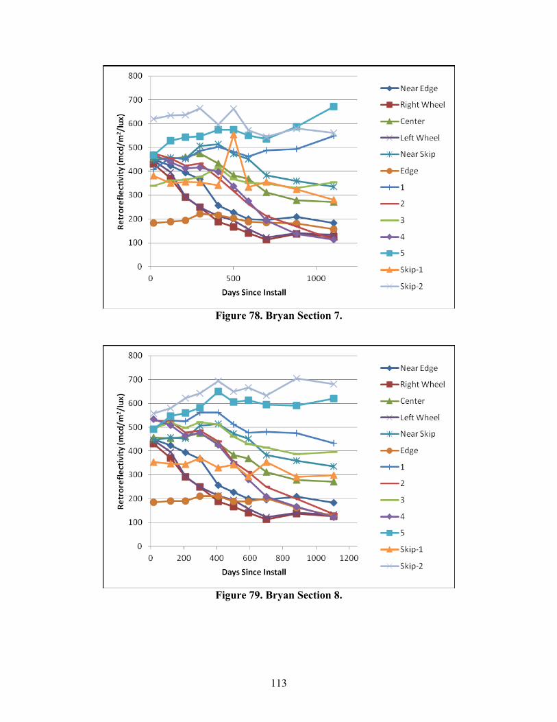
• The longline markings applied at the Bryan deck, other than those in the wheel paths

or center, did not show large changes in retroreflectivity over the duration of

evaluation. The decay rate was small, and in some cases the final retroreflectivity was

higher than the initial. This is likely the outcome of low traffic volume at the test deck

location and the fact that the service lives of the installed products are typically longer

than the evaluation period. Also, the thermoplastic materials at this deck and others

typically showed the most variation in retroreflectivity readings from one data

collection period to the other. This may be due to the nature of the intermix beads in

this pavement marking type that results in greater variations in retroreflectivity

performance as the markings age.

• Retroreflectivity data analysis indicates that the measurement points near the wheel

path have lower retroreflectivity values than the other measurement areas regardless

of being in the transverse or five- or seven-line longitudinal measurement sections for

all test decks.

• Different products have markedly different performance, which signifies the need for

field evaluation. The final retroreflectivity values are related to initial values and the

rate of decay; both vary from product to product.

• The data analysis indicated that when long lines are installed in the travel lane,

drivers did not appear to change lateral positions to avoid hitting longitudinal test

markings because of the lower retroreflectivity values on the wheel path than those on

other measurement positions. The setups of seven lines and five lines did not appear

to affect the driving path either.

• The average transverse test deck performed similarly to the average longitudinal test

deck over the 3-year evaluation period due to the fact that the points of the transverse

lines generally have high correlation with the corresponding points of the five and

seven longitudinal lines. This is particularly true when the long lines are also applied

with handcarts (transverse lines are all applied with handcarts). When long lines are

applied with long-line trucks, the correlation weakens to some degree, as found on the

Bryan deck. For the most part the individual test sections exhibited a high correlation

as well, but there were several test sections that did not show very good correlation.

70

These were typically the thermoplastic test sections that exhibited higher variability

in their retroreflectivity curves.

• At the Bryan deck, the correlation between near edge (both on transverse line or long

lines) and actual edgeline, or between near skip (both on transverse line or long lines)

and actual skip is inconclusive, with poor correlation. The poor correlation between

values from near skip locations and the actual skip location and between near edge

and actual edge could be due to the result of the slow decay in retroreflectivity values.

A positive correlation may be found when the values further decrease as the markings

age past 3 years.

RECOMMENDATIONS

Based on the results from this research, we make the following recommendations:

• If an in-lane longline test deck is to be used, the five-line design should be used. The

seven-line design does not provide additional advantages and does not capture wheel

path locations as well. This recommendation is based on strong correlation and

similar retroreflectivity values between corresponding lines.

• Transverse line decks can produce results similar to those of in-lane longline test

decks because not only are the correlations strong but the retroreflectivity values

between locations on transverse lines and corresponding long lines are similar.

• When installing field decks, comparison should be made between products that are

installed with the same application methods. This study revealed that different

application methods, extruded vs. sprayed, or handcart vs. longline truck, may affect

field performance for some PMMs.

• At the Bryan deck, results for some correlation analyses were inconclusive because

readings were rather flat during the evaluation period. When designing a test deck, a

higher ADT value is preferred. Otherwise, a longer evaluation period will need to be

adopted for durable products.

• Installation quality critically affects field performance of the PMMs. This is very

evident when comparing the performance of the same product installed by a regular

71

contract and by the research group. Quality control of installation is highly

recommended.

73

CHAPTER 6: PROVIDE DISTRICT SUPPORT FOR HURRICANE EVACUATION

ROUTING

DEVELOPMENT OF HURRICANE EVACUATION ANIMATION MAPS FOR CRP

This task concentrated on the development of animated evacuation maps for the Corpus

Christi District to facilitate the dissemination of evacuation-related information by the local print

and broadcast media. The overall goal of this effort was to provide information to the media to

facilitate improved communication of the importance of using alternate routes to I-37 in the

event of a hurricane evacuation from the region. The diversion of traffic from I-37 to alternate

routes during either an evacuation under normal traffic control, EvacuLane operation, or full

contraflow operations will result in an overall improvement in region-wide evacuation traffic

flows and reduce motorist delays. In the previous year’s activity, TTI staff developed maps that

highlighted the alternate routes to I-37 during an evacuation event. This year’s effort used those

route maps, with updates, to deliver each of the maps into animation files. These files will be

posted on TxDOT websites (such as the statewide hurricane evacuation page as well as the

District Facebook page and Twitter feeds) and can easily be uploaded to other websites as well,

such as those maintained by the local media. Corpus Christi is the first district in the state to

develop the maps in this animation format.

A unique feature of this map development is that in addition to providing an animation of

the overall evacuation trip, the maps provide zoomed-in views highlighting turns along each of

the alternate routes. As the alternate routes are different than traveling along the primary

designated evacuation route of I-37 to San Antonio, trips along the alternate routes may pass

through small towns as well as turns and roadway changes; using these routes may be

challenging to the unfamiliar motorist. The animation maps were developed for each of the five

recommended alternate routes as well as for I-37 (Figure 39).

In order to simplify the process of animation map development and to provide for

multiple uses of the route maps, the background maps were initially placed into individual slides

of PowerPoint presentations for each of the six routes. Each map identified the designated

evacuation route as highlighted; animation tools available within PowerPoint were used to move

a colored ball along the route that should be followed by the evacuating traffic. Each route was

initially shown with an overview of the route (Figure 40); the ball moves along the entire route

74

trip providing a general overview of the complete route. In some cases, route-specific

information has been provided to encourage motorists to take nonconventional routing to avoid

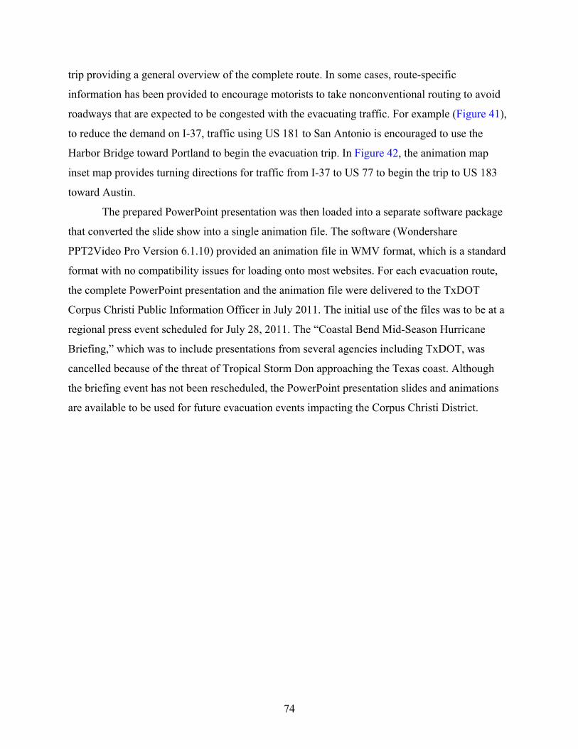
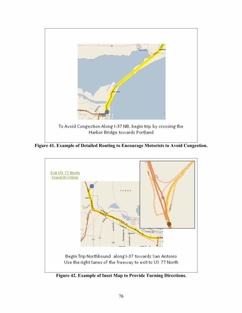
roadways that are expected to be congested with the evacuating traffic. For example (Figure 41),

to reduce the demand on I-37, traffic using US 181 to San Antonio is encouraged to use the

Harbor Bridge toward Portland to begin the evacuation trip. In Figure 42, the animation map

inset map provides turning directions for traffic from I-37 to US 77 to begin the trip to US 183

toward Austin.

The prepared PowerPoint presentation was then loaded into a separate software package

that converted the slide show into a single animation file. The software (Wondershare

PPT2Video Pro Version 6.1.10) provided an animation file in WMV format, which is a standard

format with no compatibility issues for loading onto most websites. For each evacuation route,

the complete PowerPoint presentation and the animation file were delivered to the TxDOT

Corpus Christi Public Information Officer in July 2011. The initial use of the files was to be at a

regional press event scheduled for July 28, 2011. The “Coastal Bend Mid-Season Hurricane

Briefing,” which was to include presentations from several agencies including TxDOT, was

cancelled because of the threat of Tropical Storm Don approaching the Texas coast. Although

the briefing event has not been rescheduled, the PowerPoint presentation slides and animations

are available to be used for future evacuation events impacting the Corpus Christi District.

75

Figure 39. Evacuation Routes from Corpus Christi District.

Figure 40. Initial SH 123 Evacuation Route Overview from PowerPoint.

76

Figure 41. Example of Detailed Routing to Encourage Motorists to Avoid Congestion.

Figure 42. Example of Inset Map to Provide Turning Directions.

77

CHAPTER 7: ADDITIONAL RESEARCH ACTIVITIES

85 MPH SPEED LIMIT EVALUATION

Toward the end of the fiscal year, TxDOT sought assistance in establishing criteria to

determine whether highways were designed to accommodate 80 and 85 mph posted speed limits.

This work was started and continues to be an ongoing effort that is expected to be completed

before the end of the 2011. Preliminary criteria have been selected for controlled-access

highways and conventional highways.

BRIDGE CLEARANCE SIGNING

TxDOT personnel identified the concern that sometimes a bridge clearance sign is needed

to identify a bridge that is currently not visible to a driver due to distance and is also beyond

another bridge of higher height that is within the view of the driver. The reason for needing to

identify this distant bridge at the earlier point is that it is the last exit before vehicles will

encounter this height restriction. Figure 43 shows an illustration of this situation.

78

Figure 43. Situation Illustration.

Researchers were tasked with identifying signing that would be understood by large

and/or high-profile vehicles that they needed to exit due to the height restriction at the second

bridge. Additionally, signing for use on the frontage road to discourage vehicles from entering or

re-entering the highway at the immediate downstream entrance ramp before the height restriction

was considered for this situation.

Expert Panel

To begin the process of identifying appropriate signing for the height restriction concern,

an expert panel of researchers involved in signing and human factors areas was assembled.

During the panel meetings, researchers discussed alternative information elements that would

need to be included in the sign and identified possible sign layouts. The following are the critical

information elements identified by the panel:

79

Lowest bridge height.

Distance or location information.

Action statement.

Although researchers believed that all three of these information elements were important

to drivers, there was also discussion that not all of the element may be needed to convey the

critical point to a driver. To illustrate this point, Figure 44 shows the information combinations

created within sign designs for use on the highway. Note that in some cases a distance is used on

the sign without an action (exit now) and vice versa. Researchers believed that it may be possible

for drivers to infer the need to exit without both of these information elements. However, in all

signing alternatives researchers felt that the height information was not mandatory to ensure

correct audience for the action.

Figure 44. Expert Panel Sign Alternatives.

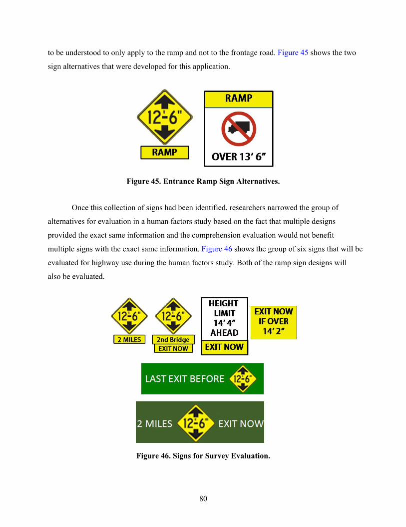
With respect to the concern of vehicles not using a specific entrance ramp to enter or re-

enter the highway, researchers developed two signing alternatives. The primary information

difference for this signing as compared to typical bridge height signing was that the sign needed

80

to be understood to only apply to the ramp and not to the frontage road. Figure 45 shows the two

sign alternatives that were developed for this application.

Figure 45. Entrance Ramp Sign Alternatives.

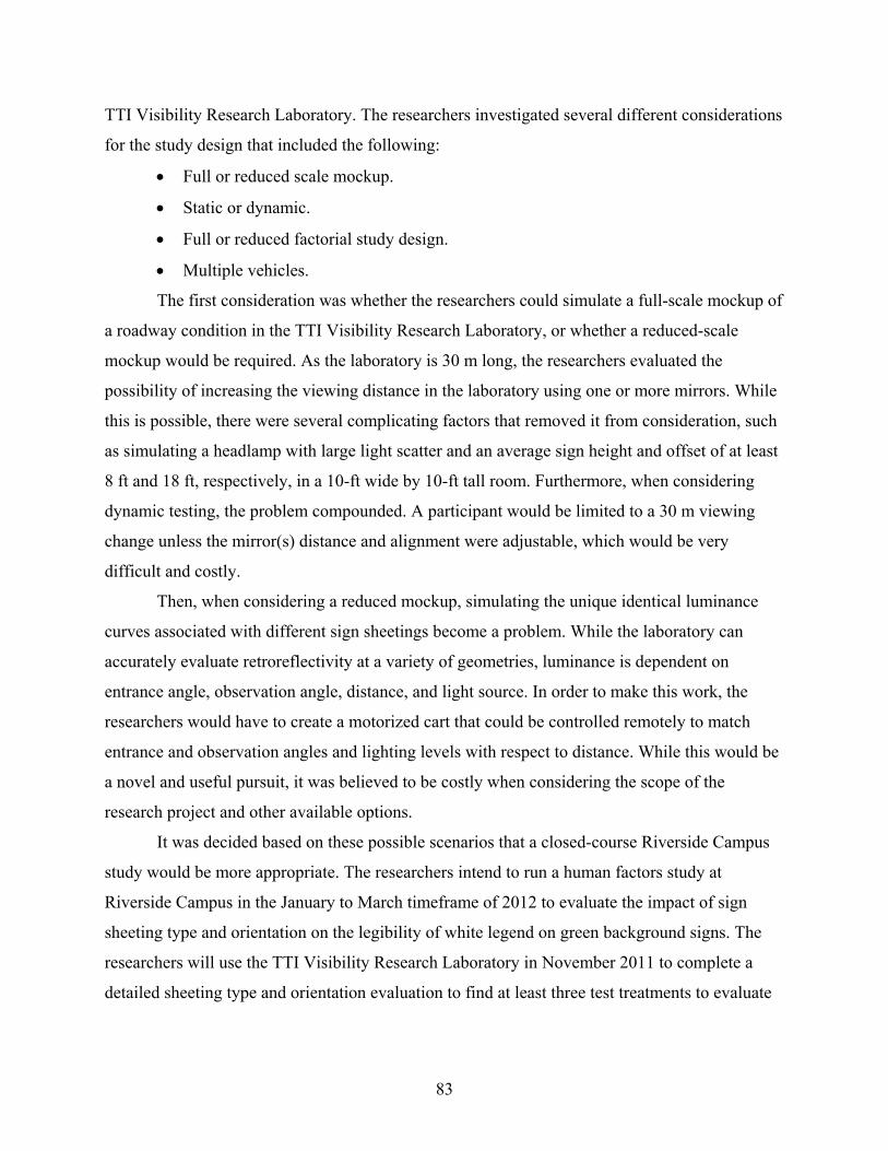
Once this collection of signs had been identified, researchers narrowed the group of

alternatives for evaluation in a human factors study based on the fact that multiple designs

provided the exact same information and the comprehension evaluation would not benefit

multiple signs with the exact same information. Figure 46 shows the group of six signs that will be

evaluated for highway use during the human factors study. Both of the ramp sign designs will

also be evaluated.

Figure 46. Signs for Survey Evaluation.

81

Experimental Design

Once the signing alternatives had been identified, researchers developed a human factors

survey experimental plan to evaluate the signs for driver comprehension and preference.

Researchers will focus on recruiting commercial drivers during this survey since they are the

primary audience of bridge height information signing.

Comprehension

Each of the sign alternatives will be displayed as a typical highway sign within a picture

showing a highway section with an exit just ahead of the driver’s current location and will have a

bridge shown in the near distance of the exit. The bridge height given on the structure using the

Texas Manual on Uniform Traffic Control Devices (MUTCD) placard sign W12-3T will be the

bridge height for the nearer structure and therefore will not match sign being evaluated. Each of

the signs being evaluated in this survey will display different heights and distances for the

downstream bridge to provide greater variety within the survey and thereby reduce redundancy

to the participant.

Each participant will view four signs to determine comprehension. This will include three

main route signs and one ramp sign. For each of these signs, participants will be asked the

following questions.

1. What information is this sign trying to tell drivers?

2. As a truck driver, what would you do if you saw this sign? Why?

Preference

At the beginning of the preference section, the survey administrator will show the

participant a diagram similar to that in Figure 43. When showing this diagram, the survey

administrator will explain to the participant the intent of the sign information to identify the

height of a downstream bridge and that they will need to exit now due to height restrictions.

Researchers will determine a preference of the participant through the use of several yes/no

questions such as “does the sign provide you with this information.” For the main line signs, the

following questions will be used.

1. There is no exit between the bridges.

2. There is no exit before the lower bridge.

82

3. You need to exit now if your truck is taller than the second bridge.

4. The information on the sign shown is not for the first bridge.

A second diagram will be used to illustrate that the vehicle is now traveling on the

frontage road as they approach an entrance onto the highway. Again, yes/no questions will be

asked to identify if the given sign provides information on the following points.

1. You should continue on the frontage road.

2. You cannot pass under a bridge on the highway.

Finally, participants will be asked if they have any suggestions to improve the signing

options they viewed during the survey.

Participant Recruitment

Researchers will recruit only commercial truck drivers for this survey. These drivers must

have a valid driver’s license and be over 18 years of age. During this survey effort researchers

plan to recruit approximately 120 surveys (60 per survey version).

Participant recruitment will be conducted at large truck stops to ensure a significant

population available of commercial drivers. The first recruitment site will be in Bryan/College

Station, Texas, on Texas Highway 6 to allow for easy access by researchers during initial data

collection and revision of survey process if necessary. Second, researchers will travel to a truck

stop near San Antonio, Texas, on I-35 to recruit a more robust population of experienced long-

haul truck drivers.

Current Task Status

Researchers have currently completed the experimental survey design and are finishing

up graphics for use during the survey. The forms to allow researchers to conduct the intended

survey task have been submitted to the Texas A&M University System Institutional Review

Board for approval. Researchers intend to conduct data collection in November/December 2011

depending upon approval timing.

ROTATIONAL SIGN SHEETING STUDY

TTI investigated the feasibility of conducting a human factors study on the impact of sign

sheeting type and orientation on the legibility of white legend on green background signs in the

83

TTI Visibility Research Laboratory. The researchers investigated several different considerations

for the study design that included the following:

Full or reduced scale mockup.

Static or dynamic.

Full or reduced factorial study design.

Multiple vehicles.

The first consideration was whether the researchers could simulate a full-scale mockup of

a roadway condition in the TTI Visibility Research Laboratory, or whether a reduced-scale

mockup would be required. As the laboratory is 30 m long, the researchers evaluated the

possibility of increasing the viewing distance in the laboratory using one or more mirrors. While

this is possible, there were several complicating factors that removed it from consideration, such

as simulating a headlamp with large light scatter and an average sign height and offset of at least

8 ft and 18 ft, respectively, in a 10-ft wide by 10-ft tall room. Furthermore, when considering

dynamic testing, the problem compounded. A participant would be limited to a 30 m viewing

change unless the mirror(s) distance and alignment were adjustable, which would be very

difficult and costly.

Then, when considering a reduced mockup, simulating the unique identical luminance

curves associated with different sign sheetings become a problem. While the laboratory can

accurately evaluate retroreflectivity at a variety of geometries, luminance is dependent on

entrance angle, observation angle, distance, and light source. In order to make this work, the

researchers would have to create a motorized cart that could be controlled remotely to match

entrance and observation angles and lighting levels with respect to distance. While this would be

a novel and useful pursuit, it was believed to be costly when considering the scope of the

research project and other available options.

It was decided based on these possible scenarios that a closed-course Riverside Campus

study would be more appropriate. The researchers intend to run a human factors study at

Riverside Campus in the January to March timeframe of 2012 to evaluate the impact of sign

sheeting type and orientation on the legibility of white legend on green background signs. The

researchers will use the TTI Visibility Research Laboratory in November 2011 to complete a

detailed sheeting type and orientation evaluation to find at least three test treatments to evaluate

84

at Riverside. The research team will provide a detailed study design in December 2011 for

review by the TxDOT project panel.

TECHNICAL SUPPORT FOR THE TEXAS MUTCD

During the development of the 2011 edition of the Texas MUTCD, TxDOT sought

technical support on several items that were identified as different from the 2009 edition of the

National MUTCD. TTI researchers provided TxDOT synthesized research results and analyses

to help support the approval of the 2011 edition of the Texas MUTCD.

TECHNICAL SUPPORT FOR TEXAS SIGN SHEETING SPECIFICATION

As a follow up to work conducted on Project 0-6384, TxDOT started to implement a

change to Department Material Specifications (DMS) 8300 to move it from an American Society

of Testing Materials (ASTM)-based specification to an American Association of State Highway

Transportation Officials (AASHTO)-based specification. As TxDOT started to make these

modifications, they sought the assistance of TTI. TTI researchers helped identify the major

AASHTO issues that would need to be addressed in a revised DMS 8300 (such as color

specifications, Type C retroreflectivity thresholds, etc.). TTI provided a set of initial

recommendations and later reviewed the specification as it was under review within the

department. The latest DRAFT specification is included below.

DMS - 8300 SIGN FACE MATERIALS

EFFECTIVE DATE: DRAFT

8300.1. Description. This Specification establishes pre-qualification, warranty, material and testing requirements, and approval procedures for the following sign face materials: • reflective sheeting, • conformable reflective sheeting, • screen inks, • colored transparent films and non-reflective black films, and • anti-graffiti films and coatings. 8300.2. Units of Measurements. The values given in parentheses (if provided) are not standard and may not be exact mathematical conversions. Use each system of units separately. Combining values from the two systems may result in nonconformance with the standard.

85

8300.3. Material Producer List. The Materials and Pavements Section of the Construction Division (CST/M&P) maintains the Material Producer List (MPL) of all materials that have demonstrated the ability to conform to the requirements of this Specification. Materials appearing on the MPL, entitled “Sign Face Materials,” do not require sampling and testing before use, but the Department may periodically sample materials to ensure conformance to this Specification and may also sample if material quality is suspect. 8300.4. Bidders’ and Suppliers’ Requirements. The Department will only purchase or allow on projects those products listed by manufacturer and product code or designation shown on the MPL. Use of pre-qualified materials does not relieve the contractor of the responsibility to provide materials that meet the specifications. 8300.5. Pre-Qualification Procedure.

A. Pre-Qualification Request. Prospective producers interested in submitting their product for evaluation must send a written request to the Texas Department of Transportation, Construction Division, Materials and Pavements Section (CP-51), 125 East 11th Street, Austin, Texas 78701-2483.

Include the following information in the request: • company name, • physical and mailing addresses, • type of material, • company material designation (product name, style number, etc.), and • contact person and telephone number. For sign sheeting submissions, include: • AASTHO M 268 sheeting type, • a test report with actual test data showing the material complies with the requirements

of AASHTO M 268 for the sheeting type proposed, and • the warranty statement required in Article 8300.6, ‘Comprehensive Manufacturer’s

Warranty Requirements.’ B. Pre-Qualification Sample. For all proposed products, provide pre-qualification sample quantities at no cost to the Department in accordance with Tex-720-I. The Department reserves the right to perform any or all tests in this Specification as a check on the tests reported by the manufacturer. In the case of any variance, the Department’s tests will govern. The Department will charge suppliers for the cost of sampling and testing of materials that do not meet the requirements of this specification in accordance with Section 8300.7.

86

C. Evaluation.

1. Qualification. The Department will list materials meeting the requirements of this Specification on the MPL.

The Department may grant provisional pre-qualification approval after successful completion of the accelerated weathering requirements; or for materials that have undergone a full evaluation by the National Transportation Product Evaluation Program, and whose test results meet the minimum durability values required by this Specification.

The Department will grant full pre-qualification after successful completion of the exterior exposure requirements. Failure to complete all exterior exposure requirements successfully is grounds for cancellation of provisional pre-qualification.

Report changes in the composition or in the manufacturing process of any material to CST/M&P at the address shown in Article 8300.4.

The Department will review significant changes reported and the material may require a re-evaluation. The Department reserves the right to conduct whatever tests deemed necessary to identify a pre-qualified material and determine if there is a change in the composition, manufacturing process, or quality, which may affect its durability or performance.

2. Failure. Producers not qualified under this Specification or removed from the MPL

may not furnish materials for Department projects and must show evidence of correction of all deficiencies before reconsideration for qualification.

Costs of sampling and testing are normally borne by the Department; however, the costs to sample and test materials failing to conform to the requirements of this Specification are borne by the supplier. This cost will be assessed at the rate established by the Director of CST/M&P and in effect at the time of testing.

Amounts due the Department will be deducted from monthly or final estimates on Contracts or from partial or final payments on direct purchases by the State.

D. Periodic Evaluation. The Department reserves the right to randomly sample and

evaluate pre-qualified materials for conformance to this Specification and to perform random audits of documentation. Department representatives may sample material from the manufacturing plant, the project site, and the warehouse. Failure of materials to comply with the requirements of this Specification as a result of periodic evaluation may be cause for removal of those materials from the MPL.

E. Disqualification. Disqualification and removal from the MPL may occur if one of the following infractions occurs:

87

• material fails to meet the requirements stated in this Specification, • the producer fails to report changes in the formulation or production process of the

material to CST/M&P, • the producer has unpaid charges for failing samples, or • the producer has unresolved warranty issues.

F. Re-Qualification. A manufacturer or supplier may submit material for re-evaluation after

one year has elapsed from the date of removal from the MPL and after documenting the problem and its resolution. Submit documentation identifying the cause and corrective action taken.

8300.6. Comprehensive Manufacturer’s Warranty Requirements. Sign face material manufacturers must comply with all requirements of the following warranty. Failure to comply with the requirements of this warranty is cause for removal from the MPL. Submit a statement indicating understanding and compliance with the provisions of the warranty and willingness to abide by the provisions to the address shown in Article 8300.4.A, ‘Pre-Qualification Request.’ Include the name, address, and telephone number of the person to contact regarding potential claims under the warranty provisions. The warranty must include the use of one manufacturer’s sign face material directly applied to a different manufacturer’s sign face material. If a failure occurs, assignment of warranty responsibility is to the manufacturer of the sign face material that fails. (Example: If the base sheeting, defined as the sheeting attached to the substrate, separates from the sign substrate, the manufacturer of the base sheeting will be responsible. If the sheeting or film used for legend detaches from the base sheeting, the manufacturer of the legend material will be responsible for the failure.)

A. Certification. Submit a certification with each lot or shipment, which states that the material supplied meets the requirements listed. Show individual lot numbers on the certification.

B. Field Performance. Sign face materials processed, applied, stored, and handled

according to the manufacturer’s recommendations (or as required in this Specification when there is an exception to the manufacturer’s recommendations), must perform satisfactorily for the number of years stated in Section 8300.6.C, “Minimum Performance Period,” for that sign face material. The performance period begins at the time of application of the base sign face material to the sign. The warranty requirements go into effect upon final acceptance by the Department. The Department will adjust the performance period to deduct the time between application of the base sign face material to the sign and Department acceptance.

The sign face material is unsatisfactory if: • it deteriorates due to natural causes to the extent that the sign is ineffective for its

intended purpose (Example: When the sign is viewed from a moving vehicle under normal day and night driving conditions), or

88

• shows any of the following defects: ▪ cracks discernible with the unaided eye from the driver’s position while in an

outside lane at a distance of 50 ft. (15 m) or greater from the sign ▪ peeling in excess of 1/4 in. (6.4 mm) ▪ shrinkage in excess of 1/8 in. (3.2 mm) total per 48 in. (1.2 m) of sheeting width ▪ fading, loss of color, or loss of reflectivity to the extent that color or reflectivity

fails to meet the requirements of AASHTO M 268. Provide the applicators with manuals, training videos, or both describing the proper application method. Submit, to the address shown in Article 8300.4.A, “Pre-Qualification Request,” a copy of the current training materials provided with any updates as they occur. Include recommended procedures for the storage and handling of materials after application to the sign face up to final installation. The sign face material manufacturer’s warranty does not relieve the Contractor for unacceptable work or improper handling, storage, or installation. The Contractor is fully responsible for all materials and work until final acceptance by the Department.

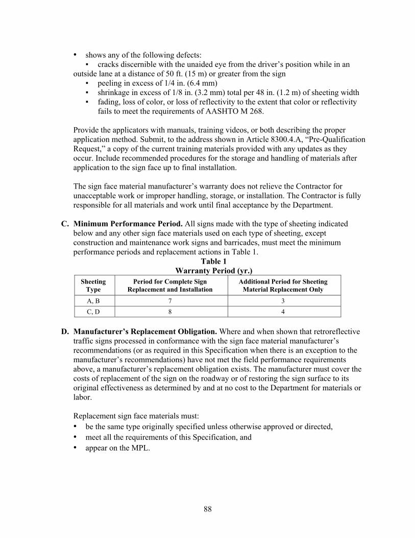
C. Minimum Performance Period. All signs made with the type of sheeting indicated

below and any other sign face materials used on each type of sheeting, except construction and maintenance work signs and barricades, must meet the minimum performance periods and replacement actions in Table 1.

Table 1 Warranty Period (yr.)

Sheeting Type

Period for Complete Sign Replacement and Installation

Additional Period for Sheeting Material Replacement Only

A, B 7 3

C, D 8 4

D. Manufacturer’s Replacement Obligation. Where and when shown that retroreflective

traffic signs processed in conformance with the sign face material manufacturer’s recommendations (or as required in this Specification when there is an exception to the manufacturer’s recommendations) have not met the field performance requirements above, a manufacturer’s replacement obligation exists. The manufacturer must cover the costs of replacement of the sign on the roadway or of restoring the sign surface to its original effectiveness as determined by and at no cost to the Department for materials or labor.

Replacement sign face materials must: • be the same type originally specified unless otherwise approved or directed, • meet all the requirements of this Specification, and • appear on the MPL.

89

Schedule with designated Department personnel, within 30 days of notification of potential replacement obligation, an on-site investigation to determine if the sign face material manufacturer’s obligation exists. Fulfill all obligations within 120 days after determination of obligations are made. The Department may replace signs where uncompleted obligations occur and may bill the manufacturer for all Department costs in performing the manufacturer’s replacement obligation. When in the judgment of the Department deteriorated signs present a traffic hazard, the Department reserves the right to remove the signs from the roadway and place them in storage for the manufacturer's inspection. Reimburse the Department for all costs, including labor for removal and replacement, when inspection reveals that a material manufacturer’s obligation exists. The materials manufacturer may use an independent Contractor to fulfill obligations to replace or refurbish signs on the roadway. Terms of the Contract must be in conformance with the provisions of Contracts used by the Department for this type work, be approved by the Department, and save harmless the Department from any liability that may arise out of the Contractor's operations. The Department can provide a sample Contract to the manufacturer upon the manufacturer’s request. The Department reserves the right to place a representative on the job to ensure that the signs are replaced or refurbished in conformance with Department standards. The Department will test all sign face materials used to fulfill the manufacturer’s obligations to ensure compliance with this Specification. Replacement material assumes the remaining warranty period of the material it replaces.

E. Sign Processors’ Obligations. Submit the following with each shipment of signs or sign

faces: • Department Contract or purchase order number and • a copy of the certification, as required in Section 8300.6.A, ‘Certification,’ showing

the lot number of all sign face materials from which the completed signs or sign faces were processed.

8300.7. Material Requirements for Reflective Sheeting. This Specification covers the general and specific requirements for the four types of reflective sheeting materials listed in AASHTO M 268—Types A, B, C, and D. The Department conducts outdoor weathering at the Department’s test site in Austin, Texas or at other locations as deemed necessary by the Director of CST/M&P.

90

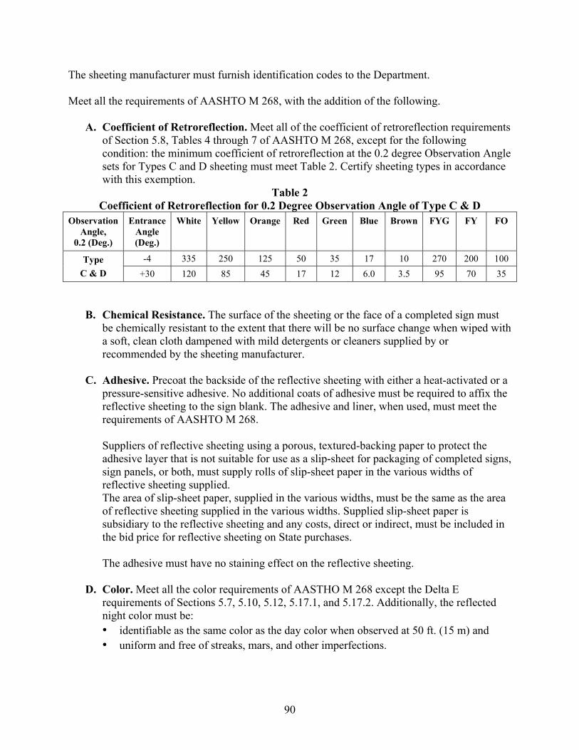
The sheeting manufacturer must furnish identification codes to the Department. Meet all the requirements of AASHTO M 268, with the addition of the following.

A. Coefficient of Retroreflection. Meet all of the coefficient of retroreflection requirements of Section 5.8, Tables 4 through 7 of AASHTO M 268, except for the following condition: the minimum coefficient of retroreflection at the 0.2 degree Observation Angle sets for Types C and D sheeting must meet Table 2. Certify sheeting types in accordance with this exemption.

Table 2 Coefficient of Retroreflection for 0.2 Degree Observation Angle of Type C & D

Observation Angle,

0.2 (Deg.)

Entrance Angle (Deg.)

White Yellow Orange Red Green Blue Brown FYG FY FO

Type C & D

-4 335 250 125 50 35 17 10 270 200 100

+30 120 85 45 17 12 6.0 3.5 95 70 35

B. Chemical Resistance. The surface of the sheeting or the face of a completed sign must be chemically resistant to the extent that there will be no surface change when wiped with a soft, clean cloth dampened with mild detergents or cleaners supplied by or recommended by the sheeting manufacturer.

C. Adhesive. Precoat the backside of the reflective sheeting with either a heat-activated or a

pressure-sensitive adhesive. No additional coats of adhesive must be required to affix the reflective sheeting to the sign blank. The adhesive and liner, when used, must meet the requirements of AASHTO M 268. Suppliers of reflective sheeting using a porous, textured-backing paper to protect the adhesive layer that is not suitable for use as a slip-sheet for packaging of completed signs, sign panels, or both, must supply rolls of slip-sheet paper in the various widths of reflective sheeting supplied. The area of slip-sheet paper, supplied in the various widths, must be the same as the area of reflective sheeting supplied in the various widths. Supplied slip-sheet paper is subsidiary to the reflective sheeting and any costs, direct or indirect, must be included in the bid price for reflective sheeting on State purchases. The adhesive must have no staining effect on the reflective sheeting.

D. Color. Meet all the color requirements of AASTHO M 268 except the Delta E

requirements of Sections 5.7, 5.10, 5.12, 5.17.1, and 5.17.2. Additionally, the reflected night color must be: • identifiable as the same color as the day color when observed at 50 ft. (15 m) and • uniform and free of streaks, mars, and other imperfections.

91

E. Screened Sheeting Optical Performance. Before exterior exposure or Weather-Ometer (WOM) exposure, sheeting reverse screened with transparent ink must have the minimum co-efficient of retroreflectivity values specified in AASHTO M 268.

(NOTE: Retroreflectivity will be determined in accordance with Tex-842-B.)

F. Material Identification. Mark each container, carton, or box containing reflective

sheeting with the information listed in AASHTO M 268. The identification numbers must also appear on the inside of the sheeting roll core. The identification number on the outside of the box and on the inside of the core must match. The mismatch of these numbers may be cause for rejection.

G. Sign Fabrication. Follow the sign fabrication requirements of AASHTO M 268,

Section 3.3.2. 8300.8. Material Requirements for Conformable Reflective Sheeting.

A. General Requirements. Conformable reflective sheeting is intended for use on both flat surface and round plastic or metal posts. Meet all the requirements of AASHTO M 268 for reflective sheeting, except when otherwise specified. In addition to the AASHTO requirements, meet the requirements of Tex-843-B.

8300.9. Material Requirements for Screen Inks.

A. General Requirements. Meet the requirements of AASHTO M 268, except when otherwise specified.

B. Color. Screen inks, when screened onto any pre-qualified white reflective sheeting, must

produce a color within the color requirements specified for the various colors of reflective sheeting in AASHTO M 268.

Use the type of screen recommended by the manufacturer. Use screen inks as supplied or thinned according to the manufacturer’s recommendations. Color will be determined by using ink from sealed, unopened containers as received from the manufacturer and according to manufacturer’s recommendations for thinning.

C. Durability. Screen inks, recommended by the ink manufacturer for use on any of the

types of reflective sheeting, must exhibit the same durability as specified for that type of reflective sheeting. When tested according to Federal Test Method 6301, “Adhesion (Wet) Tape Test,” the results must show no process inks removed after processing a minimum of 96 hr. or after exposure of the sheeting types to durability and weathering tests specified.

92

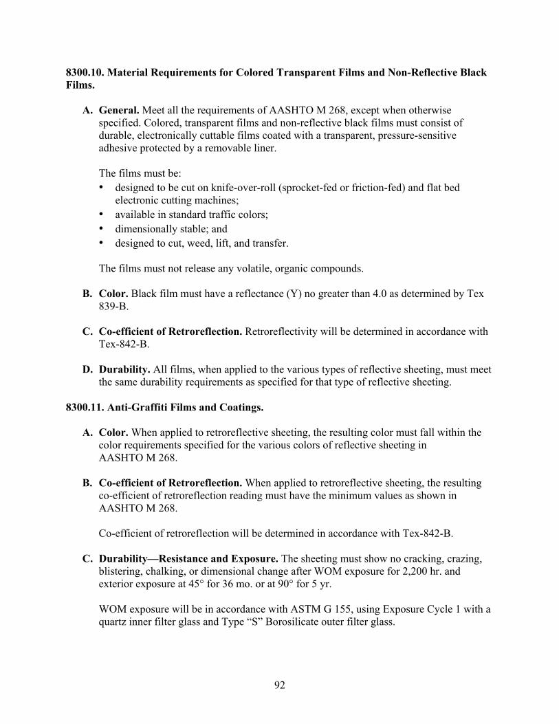
8300.10. Material Requirements for Colored Transparent Films and Non-Reflective Black Films.

A. General. Meet all the requirements of AASHTO M 268, except when otherwise specified. Colored, transparent films and non-reflective black films must consist of durable, electronically cuttable films coated with a transparent, pressure-sensitive adhesive protected by a removable liner.

The films must be: • designed to be cut on knife-over-roll (sprocket-fed or friction-fed) and flat bed

electronic cutting machines; • available in standard traffic colors; • dimensionally stable; and • designed to cut, weed, lift, and transfer. The films must not release any volatile, organic compounds.

B. Color. Black film must have a reflectance (Y) no greater than 4.0 as determined by Tex

839-B. C. Co-efficient of Retroreflection. Retroreflectivity will be determined in accordance with

Tex-842-B. D. Durability. All films, when applied to the various types of reflective sheeting, must meet

the same durability requirements as specified for that type of reflective sheeting. 8300.11. Anti-Graffiti Films and Coatings.

A. Color. When applied to retroreflective sheeting, the resulting color must fall within the color requirements specified for the various colors of reflective sheeting in AASHTO M 268.

B. Co-efficient of Retroreflection. When applied to retroreflective sheeting, the resulting

co-efficient of retroreflection reading must have the minimum values as shown in AASHTO M 268. Co-efficient of retroreflection will be determined in accordance with Tex-842-B.

C. Durability—Resistance and Exposure. The sheeting must show no cracking, crazing,

blistering, chalking, or dimensional change after WOM exposure for 2,200 hr. and exterior exposure at 45° for 36 mo. or at 90° for 5 yr. WOM exposure will be in accordance with ASTM G 155, using Exposure Cycle 1 with a quartz inner filter glass and Type “S” Borosilicate outer filter glass.

93

Exterior exposure will be facing south at the Department’s exterior exposure test site in Austin, Texas or other locations as deemed necessary by the Director of CST/M&P.

8300.12. Contrast Ratio of Sign Faces and Completed Signs. For all sign faces and completed signs using transparent screen inks or transparent films, the ‘Contrast Ratio’ is the quotient obtained when the co-efficient of retroreflection of the white is divided by the co efficient of retroreflection of the other color. The contrast ratio will be determined at an observation angle of 0.2° and an entrance angle of -4°. For all signs, which use white and red reflective sheeting, the contrast ratio must not be less than 4.0 or greater than 15.0. For all other signs, sign panels, sign faces, and traffic control devices, the contrast ratio must not be less than 4.0. 8300.13. Packaging. Package the materials in containers that will permit normal shipping and storage without the material sustaining damage or becoming difficult to apply. Roll material must contain no more than three splices per 50 yd. (46 m). The length of the roll core must not be less than the width of the material.

A. Pressure-Sensitive Material. The ends of the material must be cut square with an overlap splice of 3/8 ±1/8 in. in width (9.5 ±3.2 mm). Edges of the overlap splice are to be straight and square.

B. Heat-Activated Material. Cut the ends of the material square, but jointed closely

together and held securely in place with a removable tape.

8300.14. Archived Versions. Archived versions are available.

95

REFERENCES

1. Rose, E.R., H.G. Hawkins, Jr., A.J. Holick, and R.P. Bligh. Evaluation of Traffic Control Devices: First-Year Activities. FHWA/TX-05/0-4701-1, Texas Transportation Institute, The Texas A&M University System, College Station, Texas, October 2004.

2. Hawkins Jr., H.G., R. Garg, P.J. Carlson, and A.J. Holick. Evaluation of Traffic Control Devices: Second-Year Activities. FHWA/TX-06/0-4701-2, Texas Transportation Institute, The Texas A&M University System, College Station, Texas, October 2005.

3. Hawkins Jr., H.G., M.A. Sneed, and C.L. Williams. Evaluation of Traffic Control Devices: Third-Year Activities. FHWA/TX-07/0-4701-3, Texas Transportation Institute, The Texas A&M University System, College Station, Texas, October 2006.

4. Hawkins Jr., H.G., C.L. Williams, and S. Sunkari. Evaluation of Traffic Control Devices: Fourth-Year Activities. FHWA/TX-08/0-4701-4, Texas Transportation Institute, The Texas A&M University System, College Station, Texas, October 2007.

5. Hawkins Jr., H.G., A.M. Pike, and M. Azimi. Evaluation of Traffic Control Devices: Fifth-Year Activities. FHWA/TX-09/0-4701-5, Texas Transportation Institute, The Texas A&M University System, College Station, Texas, October 2008.

6. Carlson, P.J., R.P. Bligh, A.M. Pike, J.D. Miles, W.L. Menges, and S.C. Paulus. On-Going Evaluation of Traffic Control Devices. 0-6384-1. Texas Transportation Institute, College Station, Texas. September 2010.

7. Carlson, P.J., A.M. Pike, J.D. Miles, B.R. Ullman, R. Stevens, and D.W. Borchardt. Evaluation of Traffic Control Devices, Year 2. 9-1001-1. Texas Transportation Institute, College Station, Texas. March 2011.

8. Special Specification 8251, Reflectorized Pavement Markings with Retroreflective Requirements. Texas Department of Transportation, Austin, Texas, April 2009.

9. DMS-8220, Hot Applied Thermoplastic. Texas Department of Transportation, Austin, Texas, May 2009.

10. Traffic Control Devices on Federal-Aid and Other Streets and Highways; Color Specifications for Retroreflective Traffic Signs and Pavement Marking Materials. Federal Register, Vol 67, No. 147, Docket FHWA-99-6190, U.S. Government Printing Office, Washington, D.C., July 31, 2002, pages 49569-49575.

11. “ASTM E 1845-09 Standard Practice for Calculating Pavement Macrotexture Mean Profile Depth.” ASTM International. 2009.

12. “ASTM E 965-96 Standard Test Method for Measuring Pavement Macrotexture Depth Using a Volumetric Technique.” ASTM International. Reapproved 2006.

13. Zhang, Y., H. Ge, A.M. Pike, and P.J. Carlson. Development of Field Performance Evaluation Tools and Program for Pavement Marking Materials: Technical Report. 0-5548-1. Texas Transportation Institute, College Station, Texas. March 2011.

14. “ASTM D 713-90 Standard Practice for Conducting Road Service Tests on Fluid Traffic Marking Materials.” ASTM International. Reapproved 2010.

97

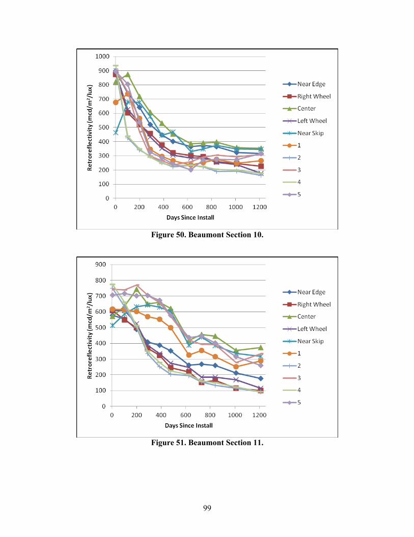
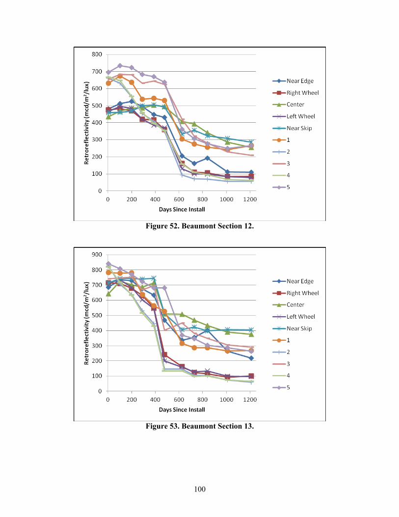
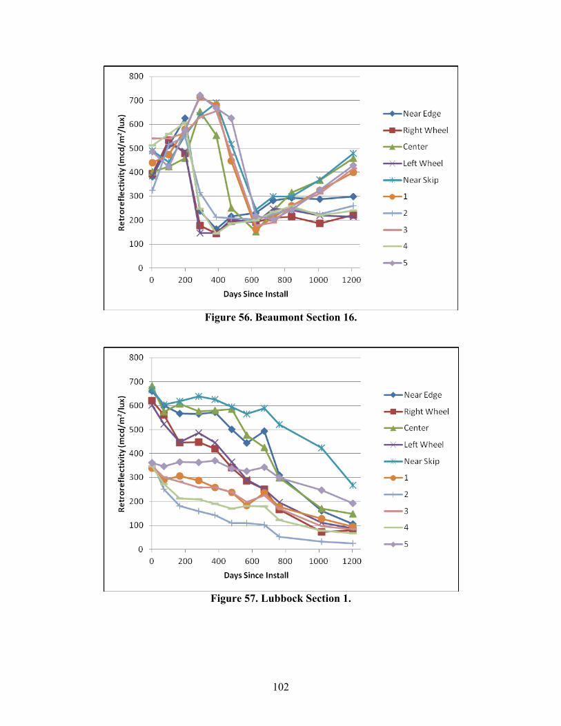
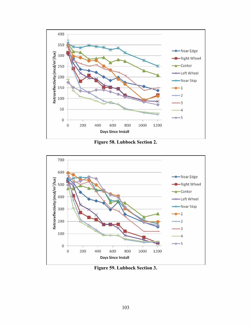
APPENDIX:

RETROREFLECTIVITY DEGREDATION CURVES FOR ALL PAVEMENT MARKING TEST DECKS

Figure 47. Beaumont Section 7.

98



99



100



101



102


Figure 57. Lubbock Section 1.

103



104



105



106



107



108



109



110

Figure 72. Bryan Section 1.


111



112



113



Date post:	05-Jul-2020
Category:	Documents
Upload:	others
View:	3 times
Download:	0 times

Evaluation of Traffic Control Devices, Year 3...Traffic Control Devices, Retroreflective Sign...

Documents