Event-triggered control: application tomobile robots

Monografia submetida a Universidade Federal de Santa Catarina

como requisito para a aprovacao da disciplina:

DAS 5511: Projeto de Fim de Curso

Marcos Cesar Bragagnolo

Florianopolis, Julho 2012

Event-triggered control: application to mobile robots

Marcos Cesar Bragagnolo

Esta monografia foi julgada no contexto da disciplinaDAS 5511: Projeto de Fim de Curso

e aprovada na sua forma final peloCurso de Engenharia de Controle e Automacao Industrial

Banca Examinadora:

Dr Romain PostoyanOrientador do Laboratorio

Professor Eugenio de Bona Castelan Neto, Dr.Orientador do curso

Acknowledge

I would like to thank my family for being so supportive during these months while

I was doing this project. To stay for such a long time away from the people we love is

not an easy task. Thank you all for the support.

I would also like to thank both my supervisors, Prof. Eugenio de Bona Castelan

and Dr. Romain Postoyan. Without their help, I would still be there trying to figure out

what to do next. It was pleasure working with you.

I would also like to thank my girlfriend, Thaise Damo. Your support during the

last weeks was amazing, and helped me keep going. I’m looking forward to see what

the future has to offer. I love you.

At last, but not least, I would like to thank all my friends. The new ones I’ve made

during my internship, the ones that showed up at my presentation, and even the ones

that couldn’t make it. You all very important to me.

This project is dedicated to all of you.

Abstract

This document presents the implementation of the event-triggered control ap-proach to a mobile robot with a nonholonomic system. Event-triggered control is atopic with great interest in the research community. Even so, there are few articlesconcerning event-triggered control applied to trajectory tracking of nonlinear systems.In this document we show this implementation, called event-triggered tracking control.

At first, we introduce the concept of a mobile robot with a nonholonomic sys-tem, explaining what a nonholonomic system is and providing the system model usedduring the project. We then define the reference system and present three different tra-jectories used during the simulations and the experiments at SAMI Benchmark. Later,we provide a bibliography study on nonholonomic systems and present Jiang and Nij-meijer’s controller, the nonlinear controller used in this project. We provide simulationsresults that shows the asymptotical convergence to the origin.

The main focus of this document is given to the event-triggered control. We startby showing a quick presentation of the event-triggered approach. Instead of using acontinuous system, we define a hybrid system where the dynamics of the robot remaincontinuous but the control inputs are sampled. This occurs because the controller isdigitally implemented and communicate with the robot via a wireless network. Withthe hybrid system, we proceed to the design of the triggering condition using Jiangand Nijmeijer’s Lyapunov function. Then, we show the proof that system does notasymptotically converge to the origin, but to a neighbourhood of the origin whose sizedepends of the parameter ε. We show the simulation results for the event-triggeredapproach validating our proof.

We finish this document providing experimental results to the control proposed.First, a time-triggered approach is implemented to serve as reference to the event-triggered approach. Later, we show the event-triggered results as well as comparisonbetween different values of σ, showing that the event-triggered approach has a goodtracking capability with much less transmissions.

Resumo Estendido

A utilizacao de sistemas de controle torna-se cada dia mais indispensavel. Seja

em uma planta quımica, uma plataforma de prospeccao de petroleo ou em um sistema

embarcado, controladores sao usados para garantir uma operacao estavel e aprimorar

a performance, em comparacao a sistemas malha aberta.

Atualmente, a grande maioria dos controladores no mercado sao implementa-

dos digitalmente. Esses controladores geralmente usam um modelo periodico, onde

tanto as medicoes quanto o sinal de controle sao atualizados a cada T segundos.

Essa abordagem tornou-se dominante pois possui analises e teoria extensivas, garan-

tindo assim robustez e performance. Ha, no entanto, uma alternativa a esse metodo

chamada Event-Triggered Control (ETC).

Event-triggered control e uma abordagem diferente do tradicional time-triggered

control pois os instantes em que o controle e atualizado nao sao mais ditados por um

perıodo, mas sim por um evento. Esse evento pode ser sinalizado de diversas manei-

ras, como por exemplo: a diferenca entre a variavel atual e o valor desejado, chegada

de uma informacao no sensor ou perturbacoes no sistema. Em geral, a grande maio-

ria dos artigos que se utilizam do ETC abordam sistemas lineares, e utilizam o event-

triggered control como um regulador de setpoint ou para seguimento de referencia.

O escopo desse projeto, no entanto, e o uso do event-triggered para seguimento de

referencia de robos nao holonomicos.

No inıcio desse projeto foi realizada uma pesquisa bibliografica, inicialmente

sobre o controle de robos moveis nao holonomicos. O objetivo dessa pesquisa ini-

cial serviu para encontrar na literatura um controlador que pudesse ser adaptado a

abordagem do ETC. Foi adotado entao o controlador projetado por Jiang e Nijmeijer,

onde utilizamos uma mudanca nas variaveis do sistema para transformar o problema

de seguimento da trajetoria em um problema de estabilizacao dos estados do sistema.

Esse controlador foi escolhido por garantir globalmente a convergencia dos estados do

robo para a referencia e por ter uma funcao de Lyapunov explıcita, a qual ajudaria na

implementacao do event-triggered. O controlador foi testado em simulacao, provando

a convergencia global dos estados do robo para a referencia.

Com o controlador escolhido, a atencao se voltou para o projeto de uma trig-

gering condition. Novamente, uma pesquisa bibliografica foi realizada para auxiliar no

projeto de uma triggering condition. Para tanto, realizar uma mudanca no nosso sis-

tema, considerando-lo um sistema hıbrido. O nosso sistema se torna hıbrido devido

a amostragem dos estados do robo. Escolheu-se entao usar duas condicoes para

decidir o evento. A primeira utiliza-se da funcao V , comparando-a com uma funcao Σ.

A segunda condicao compara uma funcao λ com uma constante ε definida durante o

projeto. Embora essa condicao nao assegura convergencia assintotica para a origem,

podemos garantir a convergencia para uma regiao proxima a origem.

Ao termino do projeto, foi a realizada a implementacao das tecnicas de controle

estudadas. O controlador projetado por Jiang e Nijmeijer foi implementado e testado

no SAMI Benchmark, e posteriormente a abordagem proposta pelo event-triggered

control foi implementada. Percebeu-se entao, uma relacao entre o numero de trans-

missoes e o valor da constante ε, onde o aumento do valor ε provoca uma diminuicao

na transmissao com o trade off de um erro maior no seguimento da referencia.

Contents

List of Figures 9

List of Tables 11

1 Introduction 12

1.1 Motivation and objectives . . . . . . . . . . . . . . . . . . . . . . . . . . 13

1.1.1 Trajectory tracking . . . . . . . . . . . . . . . . . . . . . . . . . . 13

1.1.2 Event-triggered control . . . . . . . . . . . . . . . . . . . . . . . . 13

1.2 Methodology . . . . . . . . . . . . . . . . . . . . . . . . . . . . . . . . . 14

1.3 Control and Automation Engineering Course Context . . . . . . . . . . . 14

1.4 Laboratory . . . . . . . . . . . . . . . . . . . . . . . . . . . . . . . . . . 15

1.5 Document Organization . . . . . . . . . . . . . . . . . . . . . . . . . . . 15

2 Tracking control of mobile robots 17

2.1 System Models . . . . . . . . . . . . . . . . . . . . . . . . . . . . . . . . 17

2.1.1 Robot Model . . . . . . . . . . . . . . . . . . . . . . . . . . . . . 17

2.1.2 The desired trajectory . . . . . . . . . . . . . . . . . . . . . . . . 18

2.1.2.1 The reference system . . . . . . . . . . . . . . . . . . . 18

2.1.2.2 Examples . . . . . . . . . . . . . . . . . . . . . . . . . . 19

2.2 Bibliographic Study . . . . . . . . . . . . . . . . . . . . . . . . . . . . . . 21

2.2.1 Stabilization of an equilibrium point . . . . . . . . . . . . . . . . . 22

2.2.2 Stabilization of time-varying trajectory . . . . . . . . . . . . . . . 22

2.3 Jiang and Nijmeijer’s controllers [1] . . . . . . . . . . . . . . . . . . . . . 22

2.3.1 Error system . . . . . . . . . . . . . . . . . . . . . . . . . . . . . 22

2.3.2 Controller . . . . . . . . . . . . . . . . . . . . . . . . . . . . . . . 23

2.4 Simulations . . . . . . . . . . . . . . . . . . . . . . . . . . . . . . . . . . 25

2.5 Conclusion . . . . . . . . . . . . . . . . . . . . . . . . . . . . . . . . . . 27

3 Event-triggered tracking control 28

3.1 Presentation . . . . . . . . . . . . . . . . . . . . . . . . . . . . . . . . . 28

3.2 Design of the triggering condition . . . . . . . . . . . . . . . . . . . . . . 29

3.2.1 Hybrid model . . . . . . . . . . . . . . . . . . . . . . . . . . . . . 29

3.2.2 The triggering condition . . . . . . . . . . . . . . . . . . . . . . . 30

3.3 Simulations . . . . . . . . . . . . . . . . . . . . . . . . . . . . . . . . . . 33

3.4 Conclusion . . . . . . . . . . . . . . . . . . . . . . . . . . . . . . . . . . 36

4 Implementation and experimental results 37

4.1 The SAMI benchmark . . . . . . . . . . . . . . . . . . . . . . . . . . . . 37

4.1.1 Robot: Khepera III . . . . . . . . . . . . . . . . . . . . . . . . . . 37

4.1.2 Controller-robot communication . . . . . . . . . . . . . . . . . . . 38

4.1.2.1 Orientation and Position measurement . . . . . . . . . 38

4.1.2.2 Control input . . . . . . . . . . . . . . . . . . . . . . . . 39

4.1.3 Motion Analysis . . . . . . . . . . . . . . . . . . . . . . . . . . . . 40

4.2 Implementation . . . . . . . . . . . . . . . . . . . . . . . . . . . . . . . . 40

4.3 Time-triggered controller . . . . . . . . . . . . . . . . . . . . . . . . . . . 41

4.4 Event-triggered controller . . . . . . . . . . . . . . . . . . . . . . . . . . 43

4.5 Conclusion . . . . . . . . . . . . . . . . . . . . . . . . . . . . . . . . . . 47

5 Conclusions and perspectives 48

References 49

Appendix A -- Lemmas 51

A.1 Barbalat’s lemma . . . . . . . . . . . . . . . . . . . . . . . . . . . . . . . 51

A.2 Lemma 2 . . . . . . . . . . . . . . . . . . . . . . . . . . . . . . . . . . . 51

Appendix B -- Definitions 52

B.1 L1 definition . . . . . . . . . . . . . . . . . . . . . . . . . . . . . . . . . . 52

Appendix C -- Equations 53

C.1 Equations of vr and wr for the lemniscate trajectory . . . . . . . . . . . . 53

List of Figures

1.1 Cran Logo . . . . . . . . . . . . . . . . . . . . . . . . . . . . . . . . . . . 15

2.1 A nonholonomic mechanical system . . . . . . . . . . . . . . . . . . . . 18

2.2 A diagram showing the circular trajectory . . . . . . . . . . . . . . . . . 19

2.3 A diagram showing the ellipsoidal trajectory . . . . . . . . . . . . . . . . 20

2.4 A diagram showing the lemniscate trajectory . . . . . . . . . . . . . . . 21

2.5 Trajectory and control for the circular trajectory . . . . . . . . . . . . . . 26

2.6 Trajectory and control for the ellipsoidal trajectory . . . . . . . . . . . . . 26

2.7 Trajectory and control for the lemniscate trajectory . . . . . . . . . . . . 26

3.1 Trajectory for the circular and the ellipsoidal trajectory using ETC . . . . 34

3.2 Control inputs for the circular and the ellipsoidal trajectory using ETC . . 34

3.3 Triggering condition for the circular and the ellipsoidal trajectory using ETC 35

3.4 Trajectory and control for the lemniscate trajectory using ETC . . . . . . 35

3.5 Triggering condition for the lemniscate trajectory . . . . . . . . . . . . . 35

4.1 Khepera III . . . . . . . . . . . . . . . . . . . . . . . . . . . . . . . . . . 38

4.2 Communication setup for the Khepera III . . . . . . . . . . . . . . . . . . 39

4.3 Diagram showing the time sequence of the controller . . . . . . . . . . . 40

4.4 Plot of the robot states (xe, ye, θ) of the lemniscate trajectory . . . . . . 42

4.5 Trajectory and control inputs for the circular trajectory using time-triggered

control . . . . . . . . . . . . . . . . . . . . . . . . . . . . . . . . . . . . . 42

4.6 Trajectory and control inputs for the ellipsoidal trajectory using time-

triggered control . . . . . . . . . . . . . . . . . . . . . . . . . . . . . . . 43

4.7 Trajectory and control inputs for the lemniscate trajectory using time-

triggered control . . . . . . . . . . . . . . . . . . . . . . . . . . . . . . . 43

4.8 Trajectory for the circular and the ellipsoidal trajectory using ETC . . . . 45

4.9 Control inputs for the circular and the ellipsoidal trajectory using ETC . . 45

4.10 Triggering condition for the circular and the ellipsoidal trajectory using ETC 46

4.11 Trajectory and control for the lemniscate trajectory using ETC . . . . . . 46

4.12 Triggering condition for the lemniscate trajectory . . . . . . . . . . . . . 47

List of Tables

2.1 Simulation parameters . . . . . . . . . . . . . . . . . . . . . . . . . . . . 25

3.1 Simulation parameters . . . . . . . . . . . . . . . . . . . . . . . . . . . . 33

4.1 Time-triggered control parameters . . . . . . . . . . . . . . . . . . . . . 41

4.2 Usage of the wireless transmission channel . . . . . . . . . . . . . . . . 44

12

1 Introduction

Control systems are indispensable in many high-tech systems. Whether the ap-

plication is a copier, electron microscope or oil cracker, controllers are used to guaran-

tee stable operation and enhance performance with respect to the uncontrolled, open-

loop system. The main benefits of closing the control loop are disturbance rejection

and tracking of setpoints.

Nowadays, control systems are typically digitally implemented. Mostly, time-

triggered implementations are used, in which the control task is executed periodically

in time, since for this class of control systems an extensive analysis and design theory

is available and robustness and performance criteria are well developed. Together

with the presence of programming and scheduling techniques on real-time hardware

platforms, this has become the dominating framework for digital control systems. An

alternative to this time-triggered control setup can be found in event-triggered control

systems.

In this case, signals are sampled or new control inputs are generated after the

occurrence of events, rather than after the elapse of a certain amount of time. The

underlying idea to update the control input only when it is needed. In that way, the

need for communication is expected to be significantly reduced compared to a periodic

setup. In general, the source of such an event can be based on anything. This project

presents a triggering condition based on a Lyapunov function provided by Jiang and

Nijmeijer’s controller [1] for the trajectory tracking of a nonholonomic robot.

In this chapter, the motivation and the objectives of this project are presented, as

well as the methodology used. Then, a brief description of the laboratory is provided

along with an explanation of which classes of the Control and Automation Engineer-

ing Course were essential to this project. At the end of this chapter, we provide an

explanation on how this document is organized.

13

1.1: Motivation and objectives

In the following subsections we will talk about the main topics that have motivated

this project starting with the trajectory tracking of a mobile robot. In the sequel, we talk

about the communication constraint problem and after that the main topic of interest in

this project: the event-triggered control.

1.1.1: Trajectory tracking

The control of mechanical systems with nonholonomic constraints is of great

importance for numerous practical applications, especially in the robotics field where

nonholonomics systems describe the dynamics of mobile robots and robot manipu-

lators. The control of nonholonomic systems has been the subject of considerable

research effort over the years. There are three main reasons for this trend:

• There are a large number of mechanical systems such as robot manipulators,

mobile robots, wheeled vehicles, and space and underwater robots which can be

modeled by nonholonomic dynamics;

• There is considerable challenge in the synthesis of control laws for nonholonomic

systems;

• Nonholonomic systems cannot be stabilized by continuous time-invariant control

laws.

Concerning the trajectory tracking of mobile robots, our objective is to apply

Jiang and Nijmeijer’s controller [1] to the practical experiment.

1.1.2: Event-triggered control

As technology evolves, we need to use more sensors and more actuators in a

network resulting in a increase of the required bandwidth. The classical implementation

in digital controllers uses a periodic strategy, receiving data from sensors and updating

the control every T units of time. This approach usually leads to an excessive usage

of the communication channel, which could be used more efficiently. It would be better

to close the feedback loop when needed according to the plant’s state, an approach

called event-triggered control, rather than send the control input every T units of time.

14

The main objective of this project is the implementation of the event-triggered

tracking control (ETTC) in a real nonholonomic robotic system. Using the event-

triggered approach leads to:

• Less transmissions required to stablize the system;

• Reduction in energy consumption;

• Reduce network load.

1.2: Methodology

The methodology used in the developing of this project was:

• Study of papers on Event-Triggered Control and on the tracking control of mobile

robots with nonholonomic models;

• Selection of a nonlinear feeback law and design of the associated event-triggering

condition;

• Validation of the results on simulations using Matlab;

• Implementation of the Event-Triggered Control on the mobile robot Khepera III;

• Results analysis.

The program that will be used to run the simulations is MATLAB. The interface

used to communicate with the mobile robot is implemented via a MATLAB file, making

it simpler to transfer the control used on the simulations to the real system.

1.3: Control and Automation Engineering Course Con-text

Several classes were important during the execution of this project. The control

classes like signals and linear systems, feedback systems and nonlinear systems were

very important during the study of the nonholonomic systems and the event-triggered

control, providing concepts for the development of a triggering condition and the imple-

mentation of a nonlinear controller.

15

During the implementation phase, disciplines like Computer Networks for Indus-

trial Automation and Distributed Systems were essential for the understanding of the

communication between the robot and the computer. Disciplines like Introduction to

Industrial Robotics helped the understanding of the behavior of the robot and in the

field of trajectory tracking.

1.4: Laboratory

The internship took place in the laboratory CRAN - Centre de Recherche en

Automatique de Nancy - with the supervision of Dr. Romain Postoyan, from Febru-

ary 2012 to July 2012. In this section we will present some informations about the

laboratory.

Figure 1.1: Cran Logo

Created in 1980, the CRAN is a mixed unity of research, common to the Henri

Poincare University, to the National Polytechnic Institute of Lorraine - INPL - and to the

CNRS - Centre National de la Recherche Scientifique - and it is located in the city of

Vandoeuvre, at the region of Nancy, France. Due to its multidisciplinary characteristics,

its installations are spread in several units [2].

The main lines of research at CRAN are the science of the modeling, analysis,

command and supervision of dynamic systems, signal treatment and informatics en-

gineering as well as studies in healthy engineering and system security. Today, the

laboratory has 76 professors, 6 researchers, 71 PhD students and 23 engineers.

1.5: Document Organization

In this section, the organization of this document is going to be presented.

16

In Chapter 2 we present the trajectory tracking control of mobile robots. In this

chapter the robot model is presented, as well as the theory behind nonholonomic sys-

tems, the bibliographic survey concerning linear and nonlinear controllers as well as

the theory supporting our chosen controller. Last, the simulations results of the chosen

controller are presented and commented.

In Chapter 3 the Event-Triggered Control is presented. We provide a biblio-

graphic study concerning ETC as well as the design of the triggering condition. At

the end of this chapter, simulations of the system using event-triggered control are

presented.

In Chapter 4 we present the implementation of the time-triggered and the event-

triggered approaches and compare them. We then give an overview of the hardware

and software used. We will present informations about the robot used, the type of com-

munication implemented between the robot and the computer as well as the software

and hardware used for the motion analysis of the robot. Later in this chapter, the results

of the time-triggered and event-triggered approachs are presented and compared.

In the last chapter, a conclusion for this report is provided.

17

2 Tracking control of mobilerobots

The objective of this chapter is to provide some information about the trajectory

tracking control of mobile robots. In the first section, we present the system model i. e.

the robot model and the reference system which generates the desired trajectory. In

the subsequent section, we propose a brief bibliographic study on the existing methods

for the tracking control of nonholonomic systems. Afterwards, we present the selected

control strategy and we give the main lines of the technical proof. We will end this

section with some conclusions as well as some simulation results.

2.1: System Models

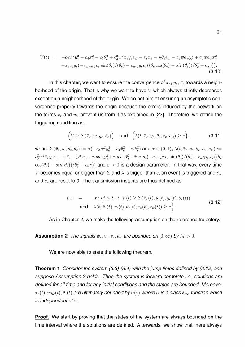
2.1.1: Robot Model

The robot dynamics are described by the following dynamical equations (as in

[3] for instance):

x = v cos(θ)

y = v sin(θ)

θ = w,

(2.1)

where (x, y) are the Cartesian coordinates and θ is the angle between the heading

direction and the x-axis. The control inputs are (v, w) and respectively represents the

linear and angular velocities. A diagram of the system is depicted in Figure 2.1.

System (2.1) is said to be nonholonomic as the controllable degrees of freedom

(DoF) are less than the total degrees of freedom of the system. That means that the

robot cannot move in a arbitrary direction because the displacement is bounded by the

orientation.

18

Figure 2.1: A nonholonomic mechanical system

2.1.2: The desired trajectory

2.1.2.1: The reference system

Our objective is to make the states of the system (2.1) track a given trajectory.

We focus on trajectories which satisfy the robot dynamics (2.1) in order to be able to

ensure asymptotic tracking properties. In that way, the desired trajectory needs to be

a solution of the following system, which we call the reference system:

xr = vr cos(θr)

yr = vr sin(θr)

θr = wr.

(2.2)

In practice, the desired trajectory is usually given as xr(t), yr(t). To show that the

trajectory satisfies (2.2), we need to find appropriate vr(t) and wr(t). With the functions

of (xr, yr) we can find their velocities (xr, yr) (provided they are differentiable) which

are vectors aligned with the x-axis and the y-axis respectively. The linear velocity vr is

found using the Pythagorean theorem, seeing that the linear velocity is the hypotenuse

while (xr, yr) are the sides of the triangle. We can find θr as a arctan() function of xrand yr while wr is the time derivative of θr. This is summarized below.

19

θr(t) = arctan( yrxr

)

vr(t) =√x2r + y2

r

wr(t) = θr,

(2.3)

2.1.2.2: Examples

We now provide examples of reference trajectories which will be considered in

the sequel.

• Circle

Figure 2.2: A diagram showing the circular trajectory

We consider a circular trajectory given as xr = xc + R sin(et) and yr = yc −R cos(et) where (xc, yc) are the coordinates of the center, R is the radius of the circle,

e is a parameter which controls the speed of the trajectory. It can be shown that the

trajectory (2.4) satisfies the equations (2.2) with

20

xr(t) = xc +R sin(et)

yr(t) = yc −R cos(et)

θr(t) = et

vr(t) = eR

wr(t) = e.

(2.4)

• Ellipse

Figure 2.3: A diagram showing the ellipsoidal trajectory

For the ellipse trajectory, we consider the following equations: xr = xc + b sin(αt)

and yr = yc− a cos(αt) where (xc, yc) are the coordinates of the center of the trajectory,

a and b are parameters used to define the semi-axis of the ellipse and α is a parameter

related to the speed of the trajectory. We can notice that if a = b the resulting function

is the same as the circular trajectory. We can see in (2.5) the remaining equations of

the ellipse:

xr(t) = xc + b sin(αt)

yr(t) = yc − a cos(αt)

θr(t) = arctan(a sin(αt)/b cos(αt))

vr(t) =√

(a2α2 sin(αt)2 + α2b2 cos(αt)2)

wr(t) =αba

+αb cos(αt)2

a sin(αt)2

b2 cos(αt)2

a2 sin(αt)2+1

.

(2.5)

21

• Lemniscate

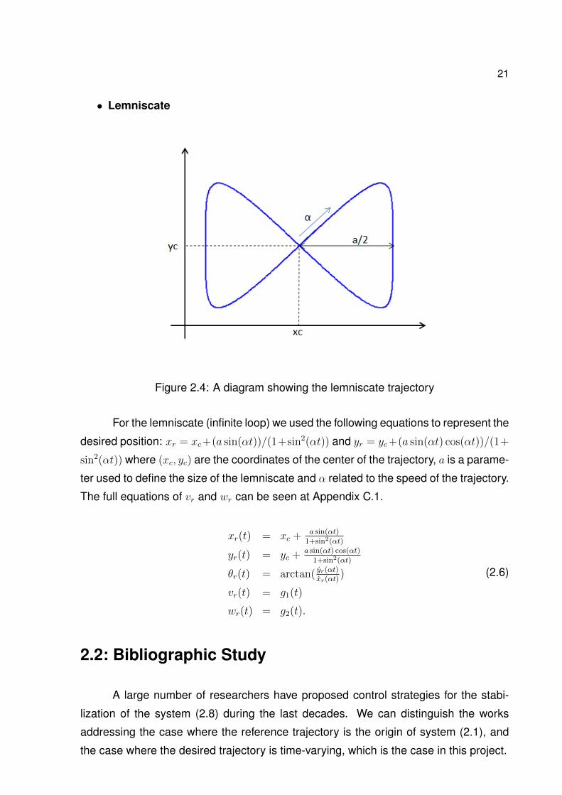
Figure 2.4: A diagram showing the lemniscate trajectory

For the lemniscate (infinite loop) we used the following equations to represent the

desired position: xr = xc+(a sin(αt))/(1+sin2(αt)) and yr = yc+(a sin(αt) cos(αt))/(1+

sin2(αt)) where (xc, yc) are the coordinates of the center of the trajectory, a is a parame-

ter used to define the size of the lemniscate and α related to the speed of the trajectory.

The full equations of vr and wr can be seen at Appendix C.1.

xr(t) = xc + a sin(αt)

1+sin2(αt)

yr(t) = yc + a sin(αt) cos(αt)

1+sin2(αt)

θr(t) = arctan( yr(αt)xr(αt)

)

vr(t) = g1(t)

wr(t) = g2(t).

(2.6)

2.2: Bibliographic Study

A large number of researchers have proposed control strategies for the stabi-

lization of the system (2.8) during the last decades. We can distinguish the works

addressing the case where the reference trajectory is the origin of system (2.1), and

the case where the desired trajectory is time-varying, which is the case in this project.

22

2.2.1: Stabilization of an equilibrium point

In some particular papers, the main objective is the stabilization of an equilibrium

point. The robot variables should thus converge to a reference position, meaning that

xr, yr and θr are constants. It has been shown that this cannot be achieved by means

of a continuous feedback, see [4], when xr, yr, θr = 0. As a consequence, a number

of techniques based on time-varying controllers and discontinuous feedbacks have

been proposed, see [5], [6], [7] and the references therein. We do not consider these

techniques because we are interested in tracking of time-varying trajectories.

2.2.2: Stabilization of time-varying trajectory

While studying the existing works on the stabilization of time-varying trajecto-

ries, it appears that a large number of articles are available (see [8], [9], [10] and the

references therein). However, very few ensures global properties (i.e. the convergence

of the robot (2.8) towards the reference system (2.2) is guaranteed for every initial

condition) together with an explicit Lyapunov function [11], [1]. We have chosen to

consider the technique in [1] because its Lyapunov-based analysis seems to be more

appropriate for the design of event-triggering condition compared to [11].

2.3: Jiang and Nijmeijer’s controllers [1]

2.3.1: Error system

As our objective is to ensure the convergence of (x, y, θ) towards (xr, yr, θr), we

naturally introduce the error variables (x − xr, y − yr, θ − θr). It has been shown in [4]

that the following change of coordinates may help for designing the controller:

xe

ye

θe

=

cos(θ) sin(θ) 0

− sin(θ) cos(θ) 0

0 0 1

xr − xyr − yθr − θ

. (2.7)

23

In that way, we derive the error system:

xe = wye − v + vr cos(θe)

ye = −wxe + vr sin(θe)

θe = wr − w.

(2.8)

Note that to write the problem using the coordinates (xe, ye, θe) is equivalent to

(xr, yr, θr) since the transformation matrix in 2.7 is invertible. On the other hand, our

tracking problem for system (2.1) has now become a stabilization one for the time-

varying system (2.8) since when (xe, ye, θe) = 0, we have x = xr, y = yr and θ = θr.

With that in mind, we will stabilize the system (2.8).

2.3.2: Controller

Before we can find a suitable controller, some variable changes are needed.

First, we define a new variable called xe:

xe := xe − c3wye, (2.9)

where c3 is a positive constant. With this new variable, we have in view of (2.8) and

(2.9)

˙xe = wye − v + vr cos(θe)− c3wye − c3w(−wxe + vr sin(θe)). (2.10)

For notational simplicity, we introduce a new variable called v1:

v1 := wye + vr cos(θe)− c3wye − c3w(−wxe + vr sin(θe)). (2.11)

We can now focus on the Lyapunov function. Let consider the following function

[1, equation (37)] with γ > 0:

V (t, xe, ye, θe) =1

2x2e +

1

2y2e +

1

2γθ2e . (2.12)

Along the solution of (2.8) and (2.10), we have:

V (t) = −c3w2y2e + xe(−yew + v1 − v) +

1

γθe[γyevr

sin(θe)

θe+ wr − w]. (2.13)

24

We can choose (v, w) as:

v = v1 + yew + c4xe, (2.14)

w = wr − γyevrsin(θe)

θe+ c5γθe, (2.15)

where c4, c5 > 0 are some design parameters. We therefore have:

V (t) = −c3w2y2e − c4x

2e − c5θ

2e . (2.16)

We cannot use (2.16) to directly conclude about the stability of the origin of

system (2.8) as V is not strictly negative when (xe, ye, θe) 6= 0.

We need to make the following assumption.

Assumption 1 Assume that vr, vr, wr, and wr are bounded on [0,∞). Furthermore,

vr(t) does not converge to zero or wr(t) does not converge to zero.

It has to be noticed that Assumption 1 is satisfied by the three examples of

reference trajectories given in Section 3.1.2.2.

We can notice that (2.16) yields the property that w(t)2ye(t)2, xe(t)2, θe(t)2 ∈

L1(0,∞) (see Appendix B.1). By assumption, the derivatives of these signals are

bounded. Hence w(t)2ye(t)2, xe(t)2 and θe(t)2 are uniformly continuous on [0,∞). With

the help of Barbalat’s lemma (see Appendix A.1), it follows that w(t)ye(t), xe(t) and θe(t)

converges to 0 as t goes to ∞. From the definition of xe in (2.9), it follows that xe(t)

goes to 0.

It remains to prove that ye(t) goes to 0. Setting η1(t) = sin(θe(t))/θe(t), we have

η1(t) going to 1 when θe = 0. In the closed-loop system , the θe system equation

becomes

θe = −c5γθe − γye(t)vr(t)η1(t). (2.17)

A direct application of Lemma 2 (see Appendix A.2) gives that γye(t)vr(t)η1(t) tends to

0. Then, we conclude that ye(t) must converge to 0.

We can then state the following proposition.

Proposition 1 (Proposition 2 in [1]) Consider system 2.8 and suppose Assumption

1 holds. Then the closed-loop solutions converge to zero i.e.

25

limt→∞

(|xe(t)|+ |ye(t)|+ |θe(t)|) = 0. (2.18)

2.4: Simulations

We provide simulation results to illustrate the efficiency of the controllers pre-

sented in Section 2.3.2. The parameters shown in this section are the same ones used

in Chapter 4 for the implementation. The reason of this choice is to make it easier for

the reader to compare the simulations with the practical results.

Circle Ellipse Lemniscate

tf 35 s 45 s 90 s

α 0 0.2 rad/s 0.1 rad/s

R 0.6 m 0 0

e 0.2 rad/s 0 0

a 0 0.8 m 1.2 m

b 0 0.5 m 0

(xc, yc) (0, 0.66) (0, 0) (0, 0)

(x(0), y(0), θ(0)) (0, 0, 0.1) (0,−0.96, 0.1) (0, 0, 0.1)

(xr(0), yr(0), θr(0)) (0, 0.066, 0) (0,−0.8, 0) (0, 0, 0.7854)

(γ, c3, c4, c5) (1, 0.7, 0.5, 0.8) (1, 0.7, 0.5, 0.8) (1, 0.7, 0.5, 0.8)

Table 2.1: Simulation parameters

As we can see in Figures 2.5, 2.6 and 2.7 the states of the robot (2.1) do asymp-

totically converge to the considered reference trajectory as ensured by Proposition 1.

In all cases we can see the control inputs (v, w) converge towards the reference veloc-

ities (vr, wr).

26

Figure 2.5: Trajectory and control for the circular trajectory

Figure 2.6: Trajectory and control for the ellipsoidal trajectory

Figure 2.7: Trajectory and control for the lemniscate trajectory

27

2.5: Conclusion

In this chapter, we have presented details about the trajectory tracking control

of class of nonholonomic systems. In the first section, the robot model was presented

along with the trajectory model and the error model, which turned the tracking prob-

lem into a stabilization problem of a time-varying system. In the subsequent section,

we have presented the bibliographic study for the trajectory tracking control problem,

showing later the controller chosen and how it was designed. At the end of this chap-

ter, we have shown the simulations results of this controller for three different reference

trajectories.

28

3 Event-triggered tracking control

In this chapter, we present the triggering condition we have developed for the

tracking control of mobile robots. In the first section, we recall the main idea of event-

triggered control and we provide a brief survey. In the subsequent section, we present

the hybrid model of the system and the triggering condition. We end this section with

some simulation results as well as some conclusions.

3.1: Presentation

Event-triggered control (ETC) consists in closing the loop according to a state-

dependent criterion. The idea is to update the control input when it is needed, as

opposed to the traditional periodic implementation. In that way, it is expected to signif-

icantly reduce the amount of transmissions needed for stabilizing the system. When

the event-triggering mechanism is designed properly, this ensures that control tasks

are executed only when necessary. Therefore, we can decrease the load in certain

resources, like a wireless network, while maintaining a desired level of performance.

Being a topic of great interest lately, ETC has been investigated for linear and nonlin-

ear systems in [12], [13], [14], [15] [16], [17]. There are fewer results which propose

a solution for the trajectory tracking problem, which is the main focus of this project.

Until this date, we are only aware of the work in [18]. As a consequence, we need to

develop an appropriate triggering condition for our problem. To solve this, we will rely

on the following articles [19], [20], [21].

29

3.2: Design of the triggering condition

3.2.1: Hybrid model

In Chapter 2, we considered the trajectory tracking control of a nonholonomic

system assuming that the control input is continuously updated. However, due to the

facts that the controller is implemented on a computer and communicate with the robot

via a wireless network, transmissions will only occur at some instants. We then have

a hybrid system i.e. a dynamical system which exhibits both continuous and discrete

dynamics. In our case, the dynamics of the robot depicted in Chapter 2 remain con-

tinuous, but the control inputs are sampled. Considering the sampling of the control

inputs at the instant t1, i ∈ Z > 0, the equation (2.8) turns into

xe(t) = w(ti)ye(t)− v(ti) + vr(t) cos(θe(t))

ye(t) = −w(ti)xe(t) + vr(t) sin(θe(t)) ∀t ∈ [ti, ti+1] .

θe(t) = wr(t)− w(ti).

(3.1)

The errors on the control input caused by the network are modelled by the following

variable

ev := v(ti)− v(t) ∀t ∈ [ti, ti+1]

ew := w(ti)− w(t).(3.2)

We can now write equation (3.1) as a full system, taking in account the dynamics

of the error (ev, ew) caused by the network:

xe = (w + ew)ye − v − ev + vr cos(θe)

ye = −(w + ew)xe + vr sin(θe)

θe = wr − w − ew ∀t ∈ [ti, ti+1]

ev = g1(t, xe, ye)

ew = g2(t, ye, θe),

(3.3)

where g1 and g2 can be deduced using (3.1) and (3.2). Traditionally, the sequence

{ti}i∈τ≥0 is defined periodically. In this project, we define it accordly to a state-dependent

criterion.

When an event is triggered, the system states (xe, ye, θe) stay the same but the

errors ev and ew on the control input are set to 0. This means an update of the control

30

input. We can see this on the following equations:

xe(t+i+1) = xe(ti+1)

ye(t+i+1) = ye(ti+1)

θe(t+i+1) = θe(ti+1)

ev(t+i+1) = 0

ew(t+i+1) = 0.

(3.4)

3.2.2: The triggering condition

To find the triggering condition for our system we now consider the hybrid system

(3.3). Consider the same function as in (2.12)

V (xe, ye, θe) =1

2x2e +

1

2y2e +

1

2γθ2e , (3.5)

where, as in (2.9)

xe = xe − c3wye, (3.6)

where c3 is a positive constant. In view of (2.10) and (3.3), we have, for t ∈ [ti, ti+1]

˙xe = wye + ewye − v − ev + vr cos(θe)− c3wye − c3w(−wxe − ewxe + vr sin(θe)). (3.7)

For notational simplicity, we are introduce the v1:

v1 = wye + vr cos(θe) + c3wye − c3w(−wxe + vr sin(θe)) (3.8)

We have, along solutions to (3.3)-(3.4), for t ∈ [ti, ti+1]

V (t) = −c3w2y2e + xe(−yew + v1 − v) + 1

γθe[γyevr

sin(θe)θe

+ wr − w]

+xe(ewye − ev + c3wew(xe) + c3wye)− yeew(xe + c3wye)− 1γθeew

+xec3ye(−ewxeγvr sin(θe)/(θe)− ewγyevr((θe cos(θe)− sin(θe))/θ2e + c5γ)

(3.9)

where (v, w) are defined by v = v1 − yew + c4xe and w = wr + γyevrsin(θe)θe

+ c5γθe as in

(2.14) and (2.15) where c4, c5 > 0 are some design parameters.

31

V (t) = −c3w2y2e − c4x

2e − c5θ

2e + c2

3w2xeyeew − evxe − 1

γθeew − c3wewy

2e + c3wewx

2e

+xec3ye(−ewxeγvr sin(θe)/(θe)− ewγyevr((θe cos(θe)− sin(θe))/θ2e + c5γ)).

(3.10)

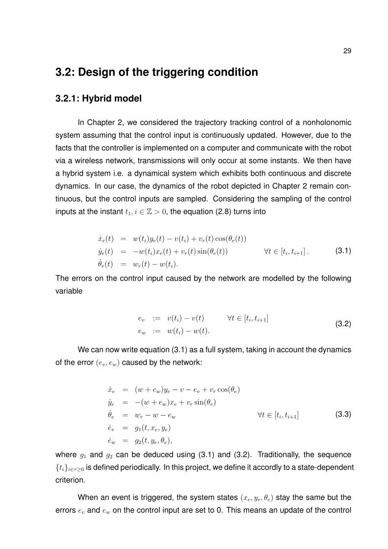
In this chapter, we want to ensure the convergence of xe, ye, θe towards a neigh-

borhood of the origin. That is why we want to have V which always strictly decreases

except on a neighborhood of the origin. We do not aim at ensuring an asymptotic con-

vergence property towards the origin because the errors induced by the network on

the terms vr and wr prevent us from it as explained in [22]. Therefore, we define the

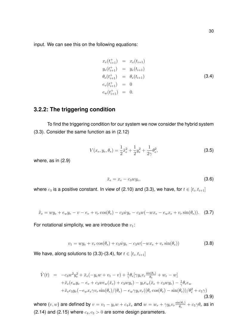
triggering condition as:(V ≥ Σ(xe, w, ye, θe)

)and

(λ(t, xe, ye, θe, ev, ew) ≥ ε

), (3.11)

where Σ(xe, w, ye, θe) := σ(−c3w2y2e − c4x

2e − c5θ

2e) and σ ∈ (0, 1), λ(t, xe, ye, θe, ev, ew) :=

c23w

2xeyeew−evxe− 1γθeew−c3wewy

2e+c3wewx

2e+xec3ye(−ewxeγvr sin(θe)/(θe)−ewγyevr((θe

cos(θe) − sin(θe))/θ2e + c5γ)) and ε > 0 is a design parameter. In that way, every time

V becomes equal or bigger than Σ and λ is bigger than ε, an event is triggered and ewand ev are reset to 0. The transmission instants are thus defined as

ti+1 = inf{t > ti : V (t) ≥ Σ(xe(t), w(t), ye(t), θe(t))

and λ(t, xe(t), ye(t), θe(t), ev(t), ew(t)) ≥ ε}.

(3.12)

As in Chapter 2, we make the following assumption on the reference trajectory.

Assumption 2 The signals wr, vr, vr, wr are bounded on [0,∞) by M > 0.

We are now able to state the following theorem.

Theorem 1 Consider the system (3.3)-(3.4) with the jump times defined by (3.12) and

suppose Assumption 2 holds. Then the system is forward complete i.e. solutions are

defined for all time and for any initial conditions and the states are bounded. Moreover

xe(t), wye(t), θe(t) are ultimately bounded by α(ε) where α is a class K∞ function which

is independent of ε.

Proof. We start by proving that the states of the system are always bounded on the

time interval where the solutions are defined. Afterwards, we show that there always

32

exists a minimum amount of time between two jumps. Then, we show that the system

is forward complete. Finally, we prove that the desired convergence property holds.

Let t0 ∈ R≥0 be the initial time and (xe(t0), ye(t0), θe(t0), ev(t0), ew(t0)) ∈ R5 be the

initial conditions. Solutions are then defined for all t ∈ [t0, t∗] where t∗ ∈ R≥0 ∪ {∞}.Consider ∆ > 0 such that |(xe(t0), ye(t0), θe(t0))| ≤ ∆. According to (3.12), we have

that, for t ∈ [ti, ti+1] ∩ [t0, t∗] with i ∈ Z≥0 (we write Σ as a function of the time for the

purpose of convenience only)

V (t) ≤ max{Σ(t), σ−1Σ(t) + ε}≤ max{Σ(t),Σ(t) + ε} = Σ(t) + ε.

(3.13)

Hence, since V (t+i ) = V (ti) for ti ∈ [0, t∗], the variables xe, ye and θe asymptotically

converge towards the set S := {(xe, w, ye, θe, ev, ew) : |Σ(xe, w, ye, θe)| ≤ ε}. As a

consequence, xe, ye and θe are bounded on [t0, t∗] by a constant which depends on

∆ and ε. By invoking the definition of w and Assumption 2, we obtain that w is also

bounded by a constant ∆ which depends on ∆, ε and M (the bound on vr and wr).

As a consequence, since ew = w(ti) − w(t), we have that ew is always bounded by

2∆. Hence, by using the facts that vr and wr are also bounded by M , we then deduce

that v is bounded by some constant ∆ which depends on ∆, ε and M and so ev is

always bounded by 2∆ in view of its definition. In that way, we have shown that for any

t ∈ [0, t∗], the states of the system (3.3)-(3.4) with the jump times defined by (3.12) are

bounded.

We now prove that there always a minimum inter-execution time τ∆,ε > 0 be-

tween two jumps. First, note that t∗ is necessarily strictly bigger t1 and t2 as the sys-

tem cannot explode before. We note that after the jump at t1, λ(t+1 ) = 0. Hence,

the next jump cannot not occur before λ increases from 0 to ε. By using the fact

that λ is continuously differentiable and that wr, wr, vr, vr are bounded by M and that

xe, ye, θe, w, v, ew, ev are all bounded by a constant N which depends on ∆, ε and M ,

we deduce that there exists N which also depends on ∆, ε and M such that for all

t ∈ [t1, t2]

|λ(t)| ≤ N . (3.14)

In that way, we see that the jump at t2 cannot occur before τ∆,ε := Nε seconds have

elapsed. In other words, t2 − t1 ≥ Nε. By iteration, we deduce that ti+1 − ti ≥ τ∆,ε for

all ti+1 ≤ t∗.

We can then show by contradiction that the system is forward complete as no

33

Zeno phenomenon can occur and all the states of the system are bounded.

Using the fact that limt→∞

sup|Σ(t)| ≤ ε, we derive, from the definition of xe, that

|xe(t)|, |wye(t)|, |θe(t)| are ultimately bounded by α(ε) where α is a class K∞ function

which is independent of ε. 2

It has to be noted that Theorem 1 does not guarantee the convergence of yetowards a neighborhood of the origin which depends on ε. We conjecture that is true

but proving it requires further investigations.

3.3: Simulations

We provide simulation results to illustrate the efficiency of the controllers using

the event-triggered condition presented in Section 3.2.2. The parameters are the same

as those used in Chapters 2 and 4, see Table 3.1. The reason of this choice is to make

it easier for the reader to compare the simulations with the experimental results. As

in practice, we will not have acess to the states of the robot at any instant, we verify

the triggering condition every T = 30 ms only, as in Chapter 4, but we only update

the control input when 3.11 holds. We acknowledge that there is a lack in our analysis.

However, the efficiency of our approach has been verified in simulations and in practice.

Circle Ellipse Lemniscate

tf 35 s 45 s 90 s

ε 0.00015 0.00015 0.00015

α 0 0.2 rad/s 0.1 rad/s

σ 0.5 0.5 0.5

R 0.6 m 0 0

e 0.2 rad/s 0 0

a 0 0.8 m 1.2 m

b 0 0.5 m 0

(xc, yc) (0, 0.66) (0, 0) (0, 0)

(x(0), y(0), θ(0)) (0, 0, 0.1) (0,−0.96, 0.1) (0, 0, 0.1)

(xr(0), yr(0), θr(0)) (0, 0.066, 0) (0,−0.8, 0) (0, 0, 0.7854)

(γ, c3, c4, c5) (1, 0.7, 0.5, 0.8) (1, 0.7, 0.5, 0.8) (1, 0.7, 0.5, 0.8)

Table 3.1: Simulation parameters

34

As we can see in Figures 3.1 and 3.4, the states of the robot (2.1) do asymptot-

ically converge to the considered reference trajectory. We can see on Figures 3.2 and

3.4 that the control inputs (v, w) are held until the next event. Figures 3.3 and 3.5 show

the instant when the transmission are triggered.

Figure 3.1: Trajectory for the circular and the ellipsoidal trajectory using ETC

Figure 3.2: Control inputs for the circular and the ellipsoidal trajectory using ETC

35

Figure 3.3: Triggering condition for the circular and the ellipsoidal trajectory using ETC

Figure 3.4: Trajectory and control for the lemniscate trajectory using ETC

Figure 3.5: Triggering condition for the lemniscate trajectory

36

3.4: Conclusion

In this chapter, we have presented details of the event-triggering condition for

the trajectory control of a mobile robot. In the first section, the main idea of event-

triggered technique was presented, and some relevant references were provided. In

the subsequent sections, we have presented the new hybrid system, showing later

the triggering condition we designed. At the end of this chapter, we have shown the

simulations results of our technique for three different reference trajectories. We are

ready to implement our event-triggered controller on the SAMI benchmark.

37

4 Implementation andexperimental results

In this chapter, we show the experimental results we have obtained. In the first

section, we present the robot, Khepera III, and its communication setup. In the next

section, we present details about the implementation, such as the time sequence of

the program executions. The next sections present the results of the time-triggered

and event-triggered approaches. We end this chapter with a comparison between

these approaches and some conclusions as well.

4.1: The SAMI benchmark

4.1.1: Robot: Khepera III

The robot we consider is the Khepera III, produced by K-Team Corporation, a

Swiss company. This robot is available in the SAMI Benchmark for educational and

research activities [3] for quite some time, proving itself to be reliable and easy to use.

This type of robot is used in more than five hundred universities and research centers

due to its modularity and multiple possibilities for control.

The model used at the ENSEM has two independent motors, five ultrasonic sen-

sors, a camera, a wireless card and a battery. We can see the details of the assembly

in Figure 4.1. Each DC motor is equipped with an incremental encoder for speed sen-

soring and is locally driven by a PID controller (responsible for tracking a given speed

reference) implemented in a PIC18F4431, using a PWM (pulse width modulation) out-

put.

The main controller (in charge of the trajectory tracking control, see Chapter 3) of

the robot is implemented on a remote computer using Matlab. This is possible thanks

to a middleware, a software layer between the operating system and the applications

38

Figure 4.1: Khepera III

on each side of a network. Using a MATLAB class called @Khepera3, the position

and the orientation of the robot are retrieved and we can set the linear and angular

velocities of the robot. In the next subsection, we explain how the remote controller

and the robot communicate.

4.1.2: Controller-robot communication

The communication between the robot and the controller happens in two dif-

ferent ways, whether measurements or control inputs are transmitted. The setup is

depicted in Figure 4.2.

4.1.2.1: Orientation and Position measurement

The sampling of the position and the orientation of the robot occurs in real

time and is sent to the controller via Ethernet and stored in a buffer (see Figure 4.2).

This buffer is located in the computer where the remote controller which we have de-

signed is located and can be acessed whenever it is required via the functions my-

39

Robot.GetXYPosition() and myRobot.GetOrientation(). This operation usually takes

less than 4 milliseconds to return the value. Given that this is actually very fast, we

consider the operating time of this function as instanteneous.

4.1.2.2: Control input

The control input (which consists of the linear velocity and angular velocity) is

sent to the robot via a Wi-Fi connection. This is done by calling the function myRobot.

-SetVelocity(v,w) on MATLAB. The robot then receives new values for v and w and

sends an acknowledgement to the computer allowing it to continue it is execution. The

main problem of this kind of transmission is that it is highly sensitive to interferences,

collisions and errors in the message.

Figure 4.2: Communication setup for the Khepera III

40

4.1.3: Motion Analysis

The robot variables (Position and Orientation) are measured thanks to the po-

sitioning system which consists of six digital cameras (called Eagle) and the motion

capture software Cortex. The software provides an interface with the cameras, allow-

ing the user to set up an environment, calibrate it and capture the motion in real-time.

The system provides a three dimensional coordinate of a marker - a high reflective

object located in the body of interest. Using the Cortex software, we can identify a set

of markers and track them in real time. The coordinates of the robot are relative to the

origin defined in the calibration step.

4.2: Implementation

As shown on Section 4.1.2, the robot and the computer have two methods of

communication. Asking for the position and the orientation of the robot takes almost

no time, while sending the control inputs to the robot takes some time. In practice, the

execution of the program on the computer is kept in a holding state until an acknowl-

edge is received. Because of this situation, we have a soft real time implementation,

in the sense that we cannot assure that each interation of the program will be finished

before a given deadline. To counter this, we measure the time elapsed between two

interactions of the program, so we can find the time elapsed between ti and ti+1, where

ti is the instant when a interaction of the program start and ti+1 the instant when this

interaction ends and another starts, even if it was not defined beforehand. Figure 4.3

shows a diagram representing this process. We consider that the start of a new inter-

ation ti is also the instant where the acknowledge was received.

Figure 4.3: Diagram showing the time sequence of the controller

41

4.3: Time-triggered controller

In this section we have implemented the Jiang and Nijmeijer’s controller pre-

sented in Chapter 2 and in a classical time-triggered fashion. The parameters used

during the experiment can be found in Table 4.1. We can see on Figures 4.5, 4.6 and

4.7 that the results obtained during the practical part are similar to the simulations in

Section 2.4.

Circle Ellipse Lemniscate

tf 35 s 45 s 90 s

α 0 0.2 rad/s 0.1 rad/s

R 0.6 m 0 0

e 0.2 rad/s 0 0

a 0 0.8 m 1.2 m

b 0 0.5 m 0

(xc, yc) (0, 0.66) (0, 0) (0, 0)

(xr(0), yr(0), θr(0)) (0, 0.066, 0) (0,−0.8, 0) (0, 0, 0.7854)

(γ, c3, c4, c5) (1, 0.7, 0.5, 0.8) (1, 0.7, 0.5, 0.8) (1, 0.7, 0.5, 0.8)

Table 4.1: Time-triggered control parameters

Once again, we can see on Figures 4.5, 4.6 and 4.7 that the states of the robot

(xe, ye, θe) asymptotically converge to a neighbourhood of the reference trajectory. We

can see in the plots to the right of Figures 4.5, 4.6 and 4.7 that the control inputs have

a lot of noise. This happens because of a measurement noise which we can see in

Figure 4.4 for the robot states (xe, ye, θ).

42

Figure 4.4: Plot of the robot states (xe, ye, θ) of the lemniscate trajectory

Figure 4.5: Trajectory and control inputs for the circular trajectory using time-triggeredcontrol

43

Figure 4.6: Trajectory and control inputs for the ellipsoidal trajectory using time-triggered control

Figure 4.7: Trajectory and control inputs for the lemniscate trajectory using time-triggered control

4.4: Event-triggered controller

In this section, we present the results given by the event-triggered controller de-

signed in Chapter 3. The parameters used can be found in Table 4.1 with the exception

of the triggering condition parameter σ. As defined in Section 3.2.2, the parameter σ

acts on the amount of transmission where σ ∈ (0, 1). As σ gets closer to 1 we expect

more transmissions compared to the case where σ is close to 0. In order to compare

the number of transmissions between each value, we define the following equation

44

usage =number of transmissions

time length. (4.1)

In Table 4.2 we can see the usage values for different σ and the values of usage

in the time-triggered implementation

Circle (tf = 35 s) Ellipse (tf = 45 s) Lemniscate (tf = 90 s)

Time-triggered 18.4571 8.8222 10.2000

σ = 0.1 0.6571 1.0889 1.4889

σ = 0.5 0.8000 1.1111 2.1000

σ = 0.9 0.9143 1.0667 2.2778

Table 4.2: Usage of the wireless transmission channel

Every real system is prone to noise, and this is the case here. In this case we

have a measurement noise (see Figure 4.4) and even though this noise does not keep

the controller from tracking the reference trajectory, it may cause unnecessary updates

of the control inputs (v, w). On the other hand, the event-triggered approach proved to

be less affected by the noises because our triggering condition λ(t, xe, ye, θe, ev, ew) ≥ ε

defined in Equation 3.11 allows us to be less sensitive to noises.

We can see in Table 4.2 that the usage grows bigger as σ approaches 1. We can

also see that the relation between the parameter σ and the usage depends highly on

the trajectory. The circular trajectory was less affected by this parameter change than

the lemniscate trajectory. The practical results provided below (Figures 4.8 and 4.11)

uses σ = 0.9 and shows a similar response compared to the time-triggered control,

correctly tracking the reference trajectory. We can also verify that the control inputs are

similar to the ones obtained during the simulations.

45

Figure 4.8: Trajectory for the circular and the ellipsoidal trajectory using ETC

Figure 4.9: Control inputs for the circular and the ellipsoidal trajectory using ETC

46

Figure 4.10: Triggering condition for the circular and the ellipsoidal trajectory usingETC

Figure 4.11: Trajectory and control for the lemniscate trajectory using ETC

47

Figure 4.12: Triggering condition for the lemniscate trajectory

In Table 4.2 we show a comparison between the four different implementations

of each trajectory. We can observe that the event-triggered approach presents the best

results regarding the usage of the wireless transmission while still maintaining a good

tracking of the reference trajectory as seen is Figures 4.8 and 4.11.

4.5: Conclusion

In this chapter, we have presented the implementation and the results for both

the time-triggered and the event-triggered implementation of Jiang and Nijmeijer’s con-

troller. In the first section, we have introduce the robot, and its details used during the

implementations. In subsequent sections, we have presented both the time-triggered

as well as the event-triggered controller. At the end of this chapter, we compare the

different values of the usage equation for each trajectory, showing the advantages of

the event-triggered approach over the time-triggered approach.

48

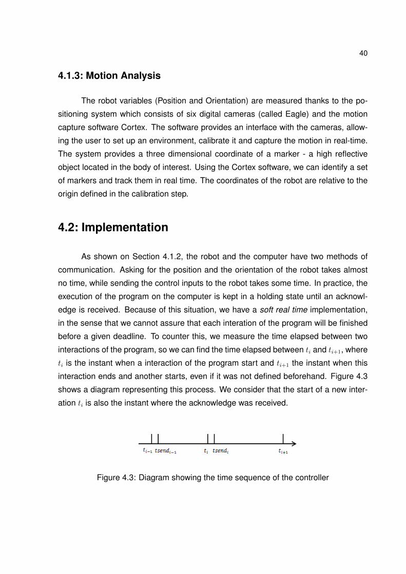
5 Conclusions and perspectives

This document has presented the implementation of the event-triggered con-

troller for a nonholonomic mobile robot on the SAMI Benchmark. The experimentation

results showed that we can maintain a good tracking property of the reference trajec-

tory with less use of the transmission channel. The triggering condition also proved to

be less sensitive to the measurement noise present at the experimentation, compared

to the time-triggered approach.

To the author of this document, the research activities developed during this

project were extremely useful to give an insight in the research world. At the start of

this project, event-triggered control was a new concept that was never treated before

during the Control and Automation Engineering Course. The same thing can be said

about the trajectory tracking control. Even though the author of this report had some

experience with path following of robotic manipulators, applying the trajectory tracking

control in a mobile robot presented its challenges.

The perspective of future work, in short term, is to redesign the triggering condi-

tion using a model-based approach. This approach was supposed to be studied during

the project, but because of the time limit of the project this approach will be studied in

a future work.

Another possible future project is to apply the knowledge acquired in this project

to the trajectory tracking control of the AR.Drone Parrot, also available at the SAMI

Benchmark. The AR.Drone Parrot is a quadricopter capable of hovering at small

heights, making it possible to track a 3 dimensional trajectory. Giving its flight ca-

pabilities, the robot model would be a more complex one with model uncertainties.

The addition of more mobile robots, turning the system into a multi-agent system,

could also provide a good background for future works. Multiple robots sharing the

same communication channel could give a useful insight on how an event-triggered

approach manages a busy multi-agent system.

49

References

[1] JIANG, Z.-P.; NIJMEIJER, H. Tracking control of mobile robots: a case study inbackstepping. Automatica, v. 33, n. 7, p. 1393–1399, 1997.

[2] CRAN, w. Serveur du CRAN. 2012. Available from internet: <http://www.cran.uhp-nancy.fr/index.html>.

[3] PIRES, L. C. A Mutiple Mobile Robots Testbed and a Game Theory Approach forCooperative Problems. 2010. UFSC.

[4] KANAYAMA, Y. et al. A stable tracking control method for an autonomous mobilerobot. In: ICRA (IEEE International Conference on Robotics and Automation). [S.l.:s.n.]. p. 384–389.

[5] KOLMANOVSKY, I.; MCCLAMROCH, N. Developments in nonholonomic controlproblems. Control Systems, IEEE, v. 15, n. 6, p. 20–36, 1995.

[6] BLOCH, A.; MCCLAMROCH, N.; REYHANOGLU, M. Controllability and stabiliz-ability properties of a nonholonomic control system. In: CDC (IEEE Conference onDecision and Control) Honolulu, U.S.A. [S.l.: s.n.]. p. 1312–1314.

[7] HESPANHA, J.; LIBERZON, D.; MORSE, A. S. Towards the supervisory controlof uncertain nonholonomic systems. In: American Control Conference. [S.l.: s.n.],1999. p. 3520–3524.

[8] BICCHI, A. et al. Closed loop smooth steering of unicycle-like vehicles. In: CDC(IEEE Conference on Decision & Control. Lake Buena Vista, FL: [s.n.], 1994. p.2455–2458.

[9] AGUIAR, A.; ATASSI, A. N.; PASCOAL, A. M. Regulation of a nonholonomic dy-namic wheeled mobile robot with parametric modeling uncertainty using lyapunovfunctions. In: CDC (IEEE Conference on Decision & Control. Sydney, Australia:[s.n.], 2000. p. 1–6.

[10] PANTELEY, E. et al. Exponential tracking control of a mobile car using a cascadedapproach. In: IFAC Workshop on Motion Control, Grenoble, France. [S.l.: s.n.]. p.221–226.

[11] LEE, T.-C. et al. Tracking control of unicycle-modeled mobile robots using a satu-ration feedback controller. IEEE Transactions on Control Systems Technology, v. 9,n. 2, p. 305–318, 2001.

[12] ARZEN, K. A simple event-based PID controller. In: 14th IFAC World Congress,Beijing, China. [S.l.: s.n.], 1999.

50

[13] ASTROM, K.; BERNHARDSSON, B. Comparison of Riemann and Lebesguesampling for first order stochastic systems. In: CDC (IEEE Conference on Decisionand Control), Las Vegas, U.S.A. [S.l.: s.n.], 2002.

[14] HEEMELS, W.; SANDEE, J.; BOSCH, P. van den. Analysis of event-driven con-trollers for linear systems. International Journal of Control, v. 81, n. 4, p. 571–590,2009.

[15] OTANEZ, G.; MOYNE, J.; TILBURY, D. Using deadbands to reduce communica-tion in networked control systems. In: ACC (American Control Conference). [S.l.:s.n.], 2002.

[16] TABUADA, P. Event-triggered real-time scheduling of stabilizing control tasks.IEEE Transactions on Automatic Control, v. 52, n. 9, p. 1680–1685, 2007.

[17] WANG, X.; LEMMON, M. Event design in event-triggered feedback control sys-tems. In: ACC (American Control Conference) Seattle, U.S.A. [S.l.: s.n.], 2008. p.3139–3144.

[18] TALLAPRAGADA, P.; CHOPRA, N. On event triggered trajectory tracking forcontrol affine nonlinear systems. In: Decision and Control and European ControlConference (CDC-ECC), 2011 50th IEEE Conference on. [S.l.: s.n.], 2011. p. 5377– 5382.

[19] ANTA, A.; TABUADA, P. Exploiting isochrony in self-triggered control. Provisionallyaccepted for publication. arXiv 1009.5208, 2011.

[20] FORNI, F. et al. Lazy sensors for the scheduling of measurement samples trans-mission in linear closed loops over networks. In: Decision and Control (CDC), 201049th IEEE Conference on. [S.l.: s.n.], 2010. p. 6469 – 6474.

[21] POSTOYAN, R. et al. A unifying Lyapunov-based framework for the event-triggered control of nonlinear systems. In: CDC / ECC (IEEE Conference on Decisionand Control and European Control Conference) Orlando, U.S.A. [S.l.: s.n.], 2011.

[22] POSTOYAN, R. et al. Emulation-based tracking solutions for nonlinear networkedcontrol systems. In: CDC (IEEE Conference on Decision and Control). Hawai,U.S.A.: [s.n.], 2012.

51

APPENDIX A -- Lemmas

A.1: Barbalat’s lemma

Lemma 1 If ϕ : R+ → R is uniformly continuous and if the limit of the integralt∫

0

ϕ(τ)dτ

exists as t→∞ and is finite then

limt→∞

ϕ(t) = 0. (A.1)

Proof 1 See Popov (1973,p. 211).

A.2: Lemma 2

Lemma 2 Consider a scalar system

x = −cx+ p(t), (A.2)

where c > 0 and p(t) is a bounded and uniformly continuous function. If, for any initial

time t0 ≥ 0 and any initial condition x(t0), the solution x(t) is bounded and converges

to 0 as t→∞ then

limt→∞

p(t) = 0. (A.3)

Proof 2 See Jiang and Nijmeijer (1996).

52

APPENDIX B -- Definitions

B.1: L1 definition

Definition 1 The set L1[0,∞) = L1 consists of all functions f : R+ → R(R+ = [0,∞)),

which are measurable and satisfy

∫ ∞0

|f(t)|1 dt <∞ (B.1)

53

APPENDIX C -- Equations

C.1: Equations of vr and wr for the lemniscate trajectory

54

v r(t

)=

√ ( aα

sin(αt)

2

sin(αt)

2+

1−

aα

cos(αt)

2

sin(αt)

2+

1+

2aα

cos(αt)

2si

n(αt)

2

(sin

(αt)

2+

1)2

) 2 +

( aα

cos(αt)

sin(αt)

2+

1−

2aα

cos(αt)

sin(αt)

2

(sin

(αt)

2+

1)2

) 2

wr(t

)=

8aα2cos(αt)3sin(αt)3

(sin(αt)2+1)3

−4aα2

cos(αt)

sin(αt)

sin(αt)2+1

+6aα2

cos(αt)

sin(αt)3

(sin(αt)2+1)2

−6aα2cos(αt)3

sin(αt)

(sin(αt)2+1)2

aα

cos(αt)

sin(αt)2+1−

2aα

cos(αt)

sin(αt)2

(sin(αt)2+1)2

aα

sin(αt)2

sin(αt)2+1−aα

cos(αt)2

sin(αt)2+1

+2aα

cos(αt)2sin(αt)2

(sin(αt)2+1)2

2

aα

cos(αt)

sin(αt)2+1−

2aα

cos(αt)

sin(αt)2

(sin(αt)2+1)2

2+

1

+

aα

sin(αt)2

sin(αt)2+1−aα

cos(αt)2

sin(αt)2+1

+2aα

cos(αt)2sin(αt)2

(sin(αt)2+1)2

2aα2sin(αt)3

(sin(αt)2+1)2

−aα2

sin(αt)

sin(αt)2+1

+8aα2cos(αt)2sin(αt)3

(sin(a

lphat)2+1)3

−6aα2cos(αt)2

sin(αt)

(sin(αt)2+1)2

a

αcos(αt)

sin(αt)2+1−

2aα

cos(αt)

sin(αt)2

(sin(αt)2+1)2

2

aα

sin(αt)2

sin(αt)2+1−aα

cos(αt)2

sin(αt)2+1

+2aα

cos(αt)2sin(αt)2

(sin(αt)2+1)2

2

aα

cos(αt)

sin(αt)2+1−

2aα

cos(αt)

sin(αt)2

(sin(αt)2+1)2

2+

1

.

(C.1

)