Abstract We show that every n × n matrix is generically a product of �n/2� + 1Toeplitz matrices and always a product of at most 2n + 5 Toeplitz matrices. Thesame result holds true if the word ‘Toeplitz’ is replaced by ‘Hankel,’ and the genericbound �n/2� + 1 is sharp. We will see that these decompositions into Toeplitz orHankel factors are unusual: We may not, in general, replace the subspace of Toeplitzor Hankel matrices by an arbitrary (2n−1)-dimensional subspace of n × n matrices.Furthermore, suchdecompositions donot exist ifwe require the factors to be symmetricToeplitz or persymmetric Hankel, even if we allow an infinite number of factors.
Keywords Toeplitz decomposition · Hankel decomposition · Linear algebraicgeometry
One of the top ten algorithms of the twentieth century [1] is the ‘decompositionalapproach to matrix computation’ [47]. The fact that a matrix may be expressed as a
Communicated by Nicholas Higham.
K. YeDepartment of Mathematics, University of Chicago, Chicago, IL 60637-1514, USAe-mail: [email protected]
L.-H. Lim (B)Computational and Applied Mathematics Initiative, Department of Statistics,University of Chicago, Chicago, IL 60637-1514, USAe-mail: [email protected]
product of a lower-triangular with an upper-triangular matrix (LU), or of an orthogonalwith an upper-triangular matrix (QR), or of two orthogonal matrices with a diagonalone (SVD) is a cornerstone of modern numerical computations. As aptly described in[47], such matrix decompositions provide a platform on which a variety of scientificand engineering problems can be solved. Once computed, they may be reused repeat-edly to solve new problems involving the original matrix and may often be updatedor downdated with respect to small changes in the original matrix. Furthermore, theypermit reasonably simple rounding-error analysis and afford high-quality softwareimplementations.
In this article, we describe a new class of matrix decompositions that differs fromthe classical ones mentioned above, but are similar in spirit. Recall that a Toeplitzmatrix is one whose entries are constant along the diagonals and a Hankel matrix isone whose entries are constant along the reverse diagonals:
T =
⎡⎢⎢⎢⎣
t0 t1 tn
t−1 t0. . .
. . .. . . t1
t−n t−1 t0
⎤⎥⎥⎥⎦ , H =
⎡⎢⎢⎢⎣
hn h1 h0. .
. h0 h−1
h1 . ..
. ..
h0 h−1 h−n
⎤⎥⎥⎥⎦
Given any n × n matrix A over C, we will show that
A = T1T2 · · · Tr , (1)
where T1, . . . , Tr are all Toeplitz matrices, and
A = H1H2 · · · Hr , (2)
where H1, . . . , Hr are all Hankel matrices. We shall call (1) a Toeplitz decompositionand (2) aHankel decomposition of A. The number r is �n/2�+1 for almost all n × nmatrices (in fact, holds generically) and is at most 4�n/2� + 5 ≤ 2n + 5 for all n × nmatrices. So every matrix can be approximated to arbitrary accuracy by a product of�n/2� + 1 Toeplitz (resp. Hankel) matrices since the set of products of �n/2� + 1Toeplitz (resp. Hankel) matrices forms a generic subset and is therefore dense (withrespect to the norm topology) in the space of n×n matrices. Furthermore, the genericbound �n/2� + 1 is sharp—by dimension counting, we see that one can do no betterthan �n/2� + 1.
The perpetual value of matrix decompositions alluded to in the first para-graph deserves some elaboration. A Toeplitz or a Hankel decomposition of agiven matrix A may not be as easily computable as LU or QR, but once com-puted, these decompositions can be reused ad infinitum for any problem involv-ing A. If A has a known Toeplitz decomposition with r factors, one can solvelinear systems in A within O(rn log2 n) time via any of the superfast algo-rithms in [2,8,17,20,27,34,36,48,56]. Nonetheless, we profess that we do notknow how to compute Toeplitz or Hankel decompositions efficiently (or stably)
123
Found Comput Math (2016) 16:577–598 579
enough for them to be practically useful. We discuss two rudimentary approachesin Sect. 7.
2 Why Toeplitz
The choice of Toeplitz factors is natural for two reasons. Firstly, Toeplitz matrices areubiquitous and are one of the most well-studied and understood classes of structuredmatrices. They arise in pure mathematics: algebra [6], algebraic geometry [46], analy-sis [31], combinatorics [35], differential geometry [40], graph theory [26], integralequations [5], operator algebra [23], partial differential equations [50], probability[45], representation theory [25], topology [42], as well as in applied mathematics:approximation theory [54], compressive sensing [32], numerical integral equations[39], numerical integration [51], numerical partial differential equations [52], imageprocessing [19], optimal control [44], quantum mechanics [24], queueing networks[7], signal processing [53], statistics [22], time series analysis [18], and among otherareas.
Furthermore, studies of related objects such as Toeplitz determinants [21], Toeplitzkernels [41], q-deformed Toeplitz matrices [29], and Toeplitz operators [12] have ledto much recent success and were behind some major developments in mathematics(e.g., Borodin–Okounkov formula for Toeplitz determinant [11]) and in physics (e.g.,Toeplitz quantization [9]).
Secondly, Toeplitz matrices have some of the most attractive computational prop-erties and are amenable to a wide range of disparate algorithms. Multiplication,inversion, determinant computation, and LU and QR decompositions of n × nToeplitz matrices may all be computed in O(n2) time and in numerically sta-ble ways. Contrast this with the usual O(n3) complexity for arbitrary matrices. Inan astounding article [8], Bitmead and Anderson first showed that Toeplitz sys-tems may in fact be solved in O(n log2 n) via the use of displacement rank; lateradvances have achieved essentially the same complexity [possibly O(n log3 n)],but are practically more efficient. These algorithms are based on a variety of dif-ferent techniques: Bareiss algorithm [20], generalized Schur algorithm [2], FFTand Hadamard product [56], Schur complement [48], semiseparable matrices [17],divide-and-concur technique [27]—the last three have the added advantage of math-ematically proven numerical stability. One can also find algorithms based on moreunusual techniques, e.g., number theoretic transforms [34] or syzygy reduction[36].
In parallel to these direct methods, we should also mention the equally substantialbody of work in iterative methods for Toeplitz matrices (cf [13,14,43] and referencestherein). These are based in part on an elegant theory of optimal circulant precondi-tioners [15,16,55], which are the most complete and well-understood class of precon-ditioners in iterative matrix computations. In short, there is a rich plethora of highlyefficient algorithms for Toeplitz matrices and the Toeplitz decomposition in (1) wouldoften (but not always) allow one to take advantage of these algorithms for generalmatrices.
123
580 Found Comput Math (2016) 16:577–598
3 Algebraic Geometry
The classical matrix decompositions1 LU, QR, and SVD correspond to the Bruhat,Iwasawa, and Cartan decompositions of Lie groups [33,37]. In this sense, LU, QR,SVD already exhaust the standard decompositions of Lie groups, and to go beyondthese, we will have to look beyond Lie theory. The Toeplitz decomposition describedin this article represents a new class of matrix decompositions that do not arise fromLie theoretic considerations, but from algebraic geometric ones.
As such, the results in this article will rely on some very basic algebraic geometry.Since we are writing for an applied and computational mathematics readership, wewill not assume any familiarity with algebraic geometry and will introduce some basicterminologies in this section. Readers interested in the details may refer to [49] forfurther information. We will assume that we are working over C.
Let C[x1, . . . , xn] denote the ring of polynomials in x1, . . . , xn with coefficients inC. For f1, . . . , fr ∈ C[x1, . . . , xn], the set
is called an algebraic set in Cn defined by f1, . . . , fr . If I is the ideal generated by
f1, . . . , fr , we also say that X is an algebraic set defined by I .It is easy to see that the collection of all algebraic sets inC
n is closed under arbitraryintersection and finite union and contains both∅ andC
n . In other words, the algebraicsets form the closed sets of a topology on C
n that we will call the Zariski topology. Itis a topology that is much coaser than the usual Euclidean or norm topology on C
n .All topological notions appearing in this article, unless otherwise specified, will bewith respect to the Zariski topology.
For an algebraic set X in Cn defined by an ideal I , the coordinate ring C[X ] of
X is the quotient ring C[x1, . . . , xn]/I ; the dimension of X , denoted dim(X), is thedimension of C[X ] as a ring. Note that dim(Cn) = n, agreeing with the usual notionof dimension. A single-point set has dimension zero.
A subset Z of an algebraic set X , which is itself also an algebraic set, is called aclosed subset of X ; it is called a proper closed subset if Z � X . An algebraic set issaid to be irreducible if it is not the union of two proper closed subsets. In this paper,an algebraic variety will mean an irreducible algebraic set and a subvariety will meanan irreducible closed subset of some algebraic set.
Let X and Y be algebraic varieties and ϕ : C[Y ] → C[X ] be a homomorphism ofC-algebras. Then, we have an induced map f : X → Y defined by
In general, a map f : X → Y between two algebraic varieties X and Y is said to be amorphism if f is induced by a homomorphism of rings ϕ : C[Y ] → C[X ]. Let f be
1 We restrict our attention to decompositions that exist for arbitrary matrices over both R and C. Of the sixdecompositions described in [47], we discounted the Cholesky (only for positive definite matrices), Schur(only over C), and spectral decompositions (only for normal matrices).
123
Found Comput Math (2016) 16:577–598 581
a morphism between X and Y . If its image is Zariski dense, i.e., f (X) = Y , then fis called a dominant morphism. If f is bijective and f −1 is also a morphism, then wesay that X and Y are isomorphic, denoted X � Y , and f is called an isomorphism.
An algebraic group is a group that is also an algebraic variety where the multipli-cation and inversion operations are morphisms.
For algebraic varieties, we have the following analogue of the open mapping the-orem in complex analysis with dominant morphisms playing the role of open maps[49].
Theorem 1 Let f : X → Y be a morphism of algebraic varieties. If f is dominant,then f (X) contains an open dense subset of Y .
A property P is said to be generic in an algebraic variety X if the points in X thatdo not have property P are contained in a proper subvariety Z of X . When we use theterm generic without specifying X , it just means that X = C
n . Formally, let Z ⊂ Xbe the subset consisting of points that do not satisfy P . If Z is a proper closed subsetof X , then we say that a point x ∈ X − Z is a generic point with respect to the propertyP , or just ‘x ∈ X − Z is a generic point,’ if the property being discussed is understoodin context. The following is an elementary, but useful fact regarding generic points.
Lemma 1 Let f : X → Y be a morphism of algebraic varieties where dim(X) ≥dim(Y ). If there is a point x ∈ X such that d fx , the differential at x, has the maximalrank dim(Y ), then d fx ′ will also have the maximal rank dim(Y ) for any generic pointx ′ ∈ X.
Proof It is obvious that d fx is of full-rank if and only if the Jacobian determinant off is nonzero at the point x . Since the Jacobian determinant of f at x is a polynomial,this means for a generic point x ′ ∈ X, d fx ′ is also of full-rank dim(Y ). ��
All notions in this section apply verbatim to the space of n × n matrices Cn×n
by simply regarding it as Cn2 , or, to be pedantic, C
n×n � Cn2 . Note that C
n×n isan algebraic variety of dimension n2 and matrix multiplication C
n×n × Cn×n →
Cn×n, (A, B) → AB, is a morphism of algebraic varieties C
2n2 and Cn2 .
4 Toeplitz Decomposition of Generic Matrices
Let Toepn(C) be the set of all n × n Toeplitz matrices with entries inC, i.e., the subsetof A = (ai, j )ni, j=1 ∈ C
n×n defined by equations
ai,i+r = a j, j+r ,
where−n+1 ≤ r ≤ n−1 and 1 ≤ r+i, r+ j, i, j ≤ n. Note that Toepn(C) � C2n−1
and that Toepn(C) is a subvariety ofCn×n . In fact, it is a linear algebraic variety definedby linear polynomials.
123
582 Found Comput Math (2016) 16:577–598
Toepn(C), being a linear subspace ofCn×n , has a natural basis Bk := (δi, j+k)
ni, j=1,
k = −n + 1,−n + 2, . . . , n − 1, i.e.,
B1 =
⎡⎢⎢⎢⎢⎣
0 1 00 1 . . .
0 . . . 0. . . 1
0
⎤⎥⎥⎥⎥⎦
, B2 =
⎡⎢⎢⎢⎢⎣
0 0 10 0 . . .
0 . . . 1. . . 0
0
⎤⎥⎥⎥⎥⎦
, . . . ,
Bn−1 =
⎡⎢⎢⎢⎢⎣
0 0 0 10 0 . . .
0 . . . 0. . . 0
0
⎤⎥⎥⎥⎥⎦
.
Note that B−k = BTk and B0 = I . A Toeplitz matrix T may thus be expressed as
T =∑n−1
j=−n+1t j B j .
Let A = (as,t ) ∈ Cn×n be arbitrary. Suppose j is a positive integer such that
j ≤ n − 1. Then, it is easy to see the effect of left- and right-multiplications of A byBj :
Bj A =
⎡⎢⎢⎢⎢⎢⎢⎢⎢⎢⎣
a j+1,1 a j+1,2 · · · a j+1,na j+2,1 a j+2,2 · · · a j+2,n
......
. . ....
an,1 an,2 · · · an,n
0 0 · · · 0...
.... . .
...
0 0 · · · 0
⎤⎥⎥⎥⎥⎥⎥⎥⎥⎥⎦
,
ABj =
⎡⎢⎢⎢⎢⎢⎢⎣
0 · · · 0 a1,1 · · · a1,n− j
0 · · · 0 a2,1 · · · a2,n− j
0 · · · 0 a3,1 · · · a3,n− j
0 · · · 0 a4,1 · · · a4,n− j. . .
......
...
0 · · · 0 an,1 · · · an,n− j
⎤⎥⎥⎥⎥⎥⎥⎦
.
Multiplying by Bj on the left has the effect of shifting a matrix up (if j is positive)or down (if j is negative) by | j | rows, whereas multiplying by Bj on the right has theeffect of shifting a matrix to right (if j is positive) or to left (if j is negative) by | j |columns.
We will denote r -tuples of n × n Toeplitz matrices by
This is an algebraic variety in Crn2 (endowed with the Zariski topology) under the
subspace topology.
Theorem 2 Let ρr : Toeprn(C) → Cn×n be the map defined by ρr (Tn−r , . . . , Tn−1) =
Tn−r · · · Tn−1. When r ≥ �n/2� + 1, for a generic point τ = (Tn−r , . . . , Tn−1) ∈Toeprn(C), the differential of ρr at τ is of full-rank n2. Therefore, for a generic A ∈Cn×n, there exists r = �n/2�+1 Toeplitz matrices T1, . . . , Tr such that A = T1 · · · Tr .
To prove this theorem, we first fix some notations. Let r = �n/2� + 1 and denote theToeplitz matrix occuring in the i th argument of ρr by
Xn−i :=∑n−1
j=−n+1xn−i, j B j , i = 1, . . . , r.
The differential of ρr at a point τ = (Tn−r , . . . , Tn−1) ∈ Toeprn(C) is the linear map(dρr )τ : Toeprn(C) → C
n × n ,
(dρr )τ (Xn−r , . . . , Xn−1) =∑r
i=1Tn−r · · · Tn−i−1Xn−i Tn−i+1 · · · Tn−1,
where Xn−i ∈ Toepn(C), i=1, . . . , r . For anygiven τ , observe that (dρr )τ (Xn−r , . . . ,
Xn−1) is an n×nmatrixwith entries that are linear forms in the xn−i, j ’s. Let L p,q be thelinear form in the (p, q)-th entry of this matrix. The statement of the theorem says thatwe can find a point τ ∈ Toeprn(C), so that these linear forms are linearly independent.For any given τ , since (dρr )τ is a linear map from the r(2n−1)-dimensional Toeprn(C)
to the n2-dimensional Cn×n , we may also regard it as an n2 × (2n − 1)r matrix M .
Hence, our goal is to find a point τ , so that this rectangular matrix M has full-rank n2;or equivalently, M has a nonzero n2 × n2 minor.
The idea of the proof of Theorem 2 is that we explicitly find such a point τ =(Tn−r , . . . , Tn−1), where the differential (dρr )τ of ρr at τ is surjective. This impliesthat the differential of ρr at a generic point is surjective, allowing us to conclude thatρr is dominant. We then apply Theorem 1 to deduce that the image of ρr contains anopen dense subset of C
n×n .As will be clear later, our choice of τ = (Tn−r , . . . , Tn−1) will take the form
where tn−i ’s are indeterminates. We will start by computing
Yn−i := Tn−r · · · Tn−i−1Xn−i Tn−i+1 · · · Tn−1.
To avoid clutter in the subsequent discussions, we adopt the following abbreviation:When we write x’s, we will mean “xn−i, j , i = 1, . . . , r, j = −n + 1, . . . , n − 1,”and when we write t’s, we will mean “tn−i , i = 1, . . . , r .” This convention will alsoapply to other lists of variables.
123
584 Found Comput Math (2016) 16:577–598
Lemma 2 For τ = (Tn−r , . . . , Tn−1) as in (3), we have
where Ω(t2) means terms of degrees at least two in t’s.
By our choice of Tn− j ’s, L p,q is a linear form in x’s with coefficients that arepolynomials in t’s. Note that L p,q has the form:
L p,q =∑r
i=1xn−i,q−p + Ω(t),
where Ω(t) denotes terms of degrees at least one in t’s.By our choice of Tn− j ’s, entries of the coefficient matrix M are also polynomials in
t’s, which implies that any n2 × n2 minor of M is a polynomial in t’s. Furthermore,observe that the constant entries (i.e., entries without t’s) in M are all 1’s. Let usexamine the coefficient of the lowest degree term of these minors.
Lemma 3 For τ = (Tn−r , . . . , Tn−1) as in (3), any n2 × n2 minor P of M is apolynomial in t’s of degree at least (n − 1)2.
Proof Let d ≤ (n − 1)2 − 1 be a positive integer. It suffices to show that any term ofdegree d in P is zero. To see this, note that theminor P is the determinant of a submatrixobtained from choosing n2 columns of M . Hence, terms of degree d < (n−1)2 comefrom taking at least 2n 1’s in M ; otherwise, the degree would be larger than or equalto (n − 1)2. If we take 2n 1’s from M , then there exist (p, q) and (p′, q ′) such thatq − p = q ′ − p′ with two of the 1’s coming from L p,q and L p′,q ′ . But terms arisingthis way must be zero because the terms determined by (p, q) and (p′, q ′) differ onlyin sign. One can see this clearly in the example immediately following this proof. ��To illustrate the proof, we consider the case n = 3 and thus r = �3/2� + 1 = 2. Inthis case,
where the rows correspond to the L p,q ’s and the columns correspond to the xn−i, j ’s.We have marked the locations of the 1’s and used ∗ to denote entries of the formΩ(t).It is easy to see in this case that if we take a 9× 9 minor of M , the degree in t’s of thisminor will be at least four. Indeed, it is also not hard to see that there exists a minorof degree exactly four—this is the content of our next lemma.
Since a linear change of variables does not change the rank of a matrix, to simplifyour calculations, we will change our x’s to y’s linearly as follows:
y j = xn−r, j + . . . + xn−1, j ,
yn−1, j = xn−r, j + . . . + xn−2, j ,
...
yn−(r−1), j = xn−r, j ,
for each −(n − 1) ≤ j ≤ n − 1.
Lemma 4 For τ = (Tn−r , . . . , Tn−1) as in (3), there exists an n2 × n2 minor P of Mthat contains a monomial term of degree exactly (n − 1)2 in t’s and whose coefficientis nonzero. It follows that rank(M) = n2 for this particular choice of τ .
Proof If we use more than 2n − 1 1’s from M to form monomials in P , then wemust obtain that coefficients of these monomials are zero. Therefore, the only way toobtain a nonzero coefficient for the degree (n − 1)2 term is to take exactly 2n − 1 1’sand (n − 1)2 terms involving t’s to the first power. We may thus ignore the Ω(t2) inLemma 2. We claim that there exists a minor of M such that it contains the monomialt2n−2n−1 t2n−2
n−2 · · · t2n−2n−r+2t
2r−3n−r+1 if n is even and t2n−2
n−1 t2n−2n−2 · · · t2n−2
n−r+2t2n−2n−r+1 if n is odd.
We will prove the odd case. The even case can be proved in the same manner. Letn = 2k + 1. Then, r = �n/2�+ 1 = k + 1 and n− r + 1 = k + 1. Upon transformingto the new coordinates y’s defined before this lemma, L p,q takes the form:
where we have adopted the convention that ti := 0 if it is not of the form tn− j withj = 1, . . . , r . The ‘· · · ’ in (4) denotes the trailing terms that play no role in theformation of the required minor P . For example, the trailing terms after tq−1y1−p,q−1are tq−2y2−p,q−2 + tq−3y3−p,q−3 + · · · + tn−r yp−q+r−n,n−r . By (4), we have tochoose exactly one 1 from the linear forms L1,q−p+1, L2,q−p+2, . . . , Ln,q−p+n , where1 ≤ q − p + j ≤ n and j = 1, . . . , n. Now, it is obvious that there is only oneway to obtain a monomial containing t2n−2
n−1 , because tn−1 only appears in L j,1 and
L j,n for j = 1, . . . , n. By the same reasoning, the monomial containing t2n−2n−1 t2n−2
n−2is unique. Continuing this procedure, we arrive at the conclusion that the monomialt2n−2n−1 t2n−2
n−2 · · · t2n−2n−r+1 is unique in P and, in particular, the coefficient of this monomial
is not zero. ��
123
586 Found Comput Math (2016) 16:577–598
To illustrate the proof of Lemma 4, we work out the case n = 5 explicitly. In thiscase, there are 25 linear forms Li, j where i, j = 1, . . . , 5. The coefficients of theselinear forms Li, j determine a matrix M of size 25 × 27. Each 25 × 25 minors of Mis a polynomial in t’s. Our goal is to find a nonzero minor P of M , and we achievethis by finding a nonzero monomial in P . Since r = �5/2� + 1 = 3, the monomialwe seek is t84 t
83 . If we backtrack the way we calculate minors of M , we would see that
to obtain a particular monomial, we need to take one coefficient from each Li, j in anappropriate way.
It is easy to see that t4 appears in L j,1 and L j,5 for j = 1, . . . , 5. Notice that we haveto take exactly one 1 from each linear form in {L p,q : −4 ≤ q − p ≤ 4} and so we areonly allowed to take eight t4’s from the ten linear forms L j,1 and L j,5, j = 1, . . . , 5,because the set {L p,q : q− p = s} contains only one element when s = −4 or 4. Next,we need to choose t3, and t3 appears only in L1, j , L2, j , L4, j , L5, j , L j,1, L j,2, L j,4as well as in L j,5. Since we have already used L j,1 and L j,5 in the previous step, weare only allowed to take t3 from L j,2, L j,4 and L1, j , L2, j , L4, j , L5, j . But by (4), they’s in L1, j , L2, j , L4, j , L5, j with coefficients involving t3 have also been used in theprevious step, compelling us to choose L j,2, L j,4.
Again, we have to take 1’s from each linear form in {L p,q : −4 ≤ q − p ≤ 4}.Therefore, we obtain t83 . Now there are five Li, j ’s left, they are L j,3 for 1 ≤ j ≤ 5,and we have to take 1 for each L j,3 since we need nine 1’s. Thus, we obtain t84 t
83 in
the unique way.The following summarizes the procedure explained above. The three tables below
are intended to show how we obtain the monomial t84 t83 . The (i, j)th entry of the three
tables indicates the term we pick from Li, j . For example, the (1, 1)th entry of thosetables means that we would pick t4 from L1,1 and the (5, 3)th entry means that wewould pick 1 from L5,3. The ‘×’ in the (1, 2)th entry of the first table indicate that wehave yet to pick an entry from L1,2. In case it is not clear, we caution the reader thatthese tables are neither matrices nor determinants.
1. We pick eight t4’s from Li,1 and L j,5 where i = 1, . . . , 4, j = 2, . . . , 5, and wepick two 1’s from L5,1 and L1,5. This yields a factor of t84 .
2. We pick eight t3’s from Li,2 and L j,4 where i = 1, . . . , 4, j = 2, . . . , 5, and wepick two 1’s from L5,2 and L4,5. This yields the factor t84 t
83 .
Li, j 1 2 3 4 51 t4 t3 × 1 12 t4 t3 × t3 t43 t4 t3 × t3 t44 t4 t3 × t3 t45 1 1 × t3 t4
123
Found Comput Math (2016) 16:577–598 587
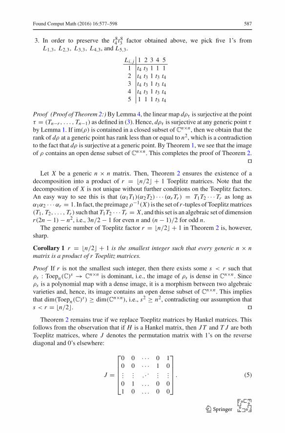
3. In order to preserve the t84 t83 factor obtained above, we pick five 1’s from
L1,3, L2,3, L3,3, L4,3, and L5,3.
Li, j 1 2 3 4 51 t4 t3 1 1 12 t4 t3 1 t3 t43 t4 t3 1 t3 t44 t4 t3 1 t3 t45 1 1 1 t3 t4
Proof (Proof of Theorem 2:)By Lemma 4, the linear map dρτ is surjective at the pointτ = (Tn−r , . . . , Tn−1) as defined in (3). Hence, dρτ is surjective at any generic point τby Lemma 1. If im(ρ) is contained in a closed subset of C
n×n , then we obtain that therank of dρ at a generic point has rank less than or equal to n2, which is a contradictionto the fact that dρ is surjective at a generic point. By Theorem 1, we see that the imageof ρ contains an open dense subset of C
n×n . This completes the proof of Theorem 2.��
Let X be a generic n × n matrix. Then, Theorem 2 ensures the existence of adecomposition into a product of r = �n/2� + 1 Toeplitz matrices. Note that thedecomposition of X is not unique without further conditions on the Toeplitz factors.An easy way to see this is that (α1T1)(α2T2) · · · (αr Tr ) = T1T2 · · · Tr as long asα1α2 · · ·αr = 1. In fact, the preimageρ−1(X) is the set of r -tuples of Toeplitzmatrices(T1, T2, . . . , Tr ) such that T1T2 · · · Tr = X , and this set is an algebraic set of dimensionr(2n − 1) − n2, i.e., 3n/2 − 1 for even n and (n − 1)/2 for odd n.
The generic number of Toeplitz factor r = �n/2� + 1 in Theorem 2 is, however,sharp.
Corollary 1 r = �n/2� + 1 is the smallest integer such that every generic n × nmatrix is a product of r Toeplitz matrices.
Proof If r is not the smallest such integer, then there exists some s < r such thatρs : Toepn(C)s → C
n×n is dominant, i.e., the image of ρs is dense in Cn×n . Since
ρs is a polynomial map with a dense image, it is a morphism between two algebraicvarieties and, hence, its image contains an open dense subset of C
n×n . This impliesthat dim(Toepn(C)s) ≥ dim(Cn×n), i.e., s2 ≥ n2, contradicting our assumption thats < r = �n/2�. ��
Theorem 2 remains true if we replace Toeplitz matrices by Hankel matrices. Thisfollows from the observation that if H is a Hankel matrix, then JT and T J are bothToeplitz matrices, where J denotes the permutation matrix with 1’s on the reversediagonal and 0’s elsewhere:
J =
⎡⎢⎢⎢⎢⎣
0 0 · · · 0 10 0 · · · 1 0...
... . .. ...
...
0 1 . . . 0 01 0 . . . 0 0
⎤⎥⎥⎥⎥⎦
. (5)
123
588 Found Comput Math (2016) 16:577–598
Note that J 2 = I . Let X = T1 · · · Tr be a Toeplitz decomposition of a genericmatrix X . If r is even, then
X = (T1 J )(JT2) · · · (Tr−1 J )(JTr )
is a Hankel decomposition of X . If r is odd, then
J X = (JT1)(T2 J )(JT3) · · · (Tr−1 J )(JTr )
is a Hankel decomposition of J X . Since J is invertible, ifU ⊆ Cn×n is a Zariski open
subset, then so is the set JU . This implies that a generic matrix may always be writtenas a product of r Hankel matrices. We would like to thank an anonymous referee ofthis paper for providing this argument, vastly simplifying our original proof.
Although we have been working over C for convenience, Theorem 2 and Corol-lary 1 (as well as their Hankel analogues) hold over any algebraically closed field, forexample, the algebraic numbers Q or the field of Puiseux series over C. Indeed, Theo-rem 1 is true for any morphism of schemes over an integral domain (see, for example,[49]) and Lemma 1 is true over any infinite perfect field (see, for example, [28]). Inother words, the two results that we use in our proofs here hold over algebraicallyclosed fields.
Moreover, even though the proof of Theorem 2 requires algebraic closure, if weonly consider the dominance and surjectivity of ρr as a morphism of schemes, thenour results are true over any infinite field of characteristic zero since Theorem 1 andLemma 1 hold in this case. For example, it is true that the image of ρr contains anopen subscheme of C
n×n , but this does not imply that a generic matrix is the productof r Toeplitz matrices. The reason being that for a non-algebraically field k, thereis no one-to-one correspondence between closed points of Spec(k[x1, . . . , xn]) andelements of k
n (such a correspondence exists for an algebraically closed field).
5 Toeplitz Decomposition of Arbitrary Matrices
We now show that every invertible n × n matrix is a product of 2r Toeplitz matricesand every matrix is a product of 4r + 1 Toeplitz matrices, where r = �n/2� + 1.
We make use of the following property of algebraic groups [10].
Lemma 5 Let G be an algebraic group and U, V be two open dense subsets of G.Then, UV = G.
Proposition 1 Let W be a subspace of Cn × n such that the map ρ : Wr → C
n × n isdominant. Then, every invertible n × n matrix can be expressed as the product of 2melements in W.
Proof Since ρ is dominant, im(ρ) contains an open dense subset ofCn×n . On the other
hand, GLn(C) is an open dense subset of Cn×n ; therefore, im(ρ) contains an open
dense subset of GLn(C). Let U be such an open dense subset. Then, by Lemma 5,we see that UU = GLn(C). Hence, every invertible matrix A can be expressed as a
123
Found Comput Math (2016) 16:577–598 589
product of two matrices in U and so A can be expressed as a product of 2m matricesin W . ��Corollary 2 Every invertible n×n matrix can be expressed as a product of 2r Toeplitzmatrices.
Proof By Theorem 2, we have seen that the map ρ is dominant. Hence, by Proposi-tion 1, every invertible matrix is a product of 2r Toeplitz matrices. ��Lemma 6 Let W be a linear subspace of C
n×n such that ρ : Wr → Cn×n is
dominant. Let A ∈ Cn×n and suppose the orbit of A under the action of GLn(C) ×
GLn(C), acting by left and right matrix multiplication, intersects W. Then, A can beexpressed as a product of 4m + 1 matrices in W.
Proof By assumption, there exist invertiblematrices P, Q such that A = PBQ, whereB ∈ W . By Proposition 2, we know that P, Q can be decomposed into a product of rmatrices in W . Hence, A can be expressed as a product of 4m + 1 matrices in W . ��Theorem 3 Every n × n matrix can be expressed as a product of 4r + 1 Toeplitzmatrices for r = �n/2� + 1.
Proof It remains to consider the rank-deficient case. Let A be an n× n matrix of rankm < n. Then, there exist invertible matrices P, Q such that A = PBn−mQ, whereBk = (δi+k, j ) for k = 1, . . . , n − 1. By Lemma 6, A is a product of 4r + 1 Toeplitzmatrices. ��
It is easy to see that 4r +1 is not the smallest integer p such that every n×n matrixis a product of p Toeplitz matrices. For example, consider the case n = 2. If we set
[x yz x
] [s tu s
]=
[a bc d
],
where x, y, z, s, t , and u are unknowns; a simple calculation shows that when c =b = 0, we have a solution
Hence, any 2 × 2 matrix requires two Toeplitz factors to decompose.While the generic bound r = �n/2�+1 is sharp by Corollaries 1, we see no reason
that the bound 4r + 1 in Theorem 3 should also be sharp. In fact, we are optimisticthat the generic bound r holds always:
123
590 Found Comput Math (2016) 16:577–598
Conjecture 1 Every matrix A ∈ Cn×n is a product of at most �n/2� + 1 Toeplitz
matrices.
The discussion in this section clearly also applies to Hankel decomposition.
6 Toeplitz Decomposition is Special
We will see in this section that the Toeplitz decomposition studied above are excep-tional in two ways: (1) The Toeplitz structure of the factors cannot be extended toarbitrary structured matrices that form a (2n−1)-dimensional subspace of C
n × n , and(2) the Toeplitz structure of the factors cannot be further restricted to circulant, sym-metric Toeplitz, or persymmetric Hankel. Moreover, (1) and (2) hold even if we allowan infinite number of factors in the decomposition. For (2), one may immediately ruleout circulant matrices since these are closed under multiplication although the othertwo structures might seem plausible at first.
Noting that Toepn(C) is a (2n − 1)-dimensional subspaces of Cn × n , one might
suspect that such decompositions are nothing special and would hold for any subspaceW ⊆ C
n × n of dimension 2n−1. This is not the case. In fact, for any d = 1, . . . , n2−n + 1, we may easily construct a d-dimensional subspace W ⊆ C
n × n such that adecomposition of an arbitrary matrix into products of r elements of W does not existfor any r ∈ N. For example, W could be taken to be any d-dimensional subspace ofCn×n consisting of matrices of the form
⎡⎢⎢⎣
∗ ∗ · · · ∗0 ∗ · · · ∗...
.... . .
...
0 ∗ · · · ∗
⎤⎥⎥⎦ ,
i.e., with zeros below the (1, 1)th entry. Since such a structure is preserved undermatrix product, the semigroup generated byW , i.e., the set of all products of matricesfrom W , could never be equal to all of C
n×n .While here we are primarily concern with the semigroup generated by a subspace,
it is interesting to also observe the following.
Proposition 2 Let W be a proper associative subalgebra (with identity) of Cn × n.
Then, dimW ≤ n2 − n + 1.
Proof Every associative algebra can be made into a Lie algebra by defining the Liebracket as [X,Y ] = XY − Y X . So W may be taken to be a Lie algebra. Let sln(C)
be the Lie algebra of traceless matrices. For any X ∈ W , we can write
X = X0 + tr(X)
nI,
where tr(X) is the trace of X , X0 is an element in sln(C), and I is the identity matrix.In particular, X0 ∈ W since both I and X are in W . Hence, we have
W = (W ∩ sln(C)) ⊕ C · I.
123
Found Comput Math (2016) 16:577–598 591
Since W ∩ sln(C) is a proper Lie subalgebra of sln(C) and the dimension of aproper Lie subalgebra of sln(C) cannot exceed n2 − n [3], we must have
dimW ≤ n2 − n + 1.
��On the other hand, onemight perhaps think that any n × nmatrix is expressible as a
product of n symmetric Toeplitz matrices (note that these require exactly n parametersto specify and form an n-dimensional linear subspace of Toepn(C)). We see belowthat this is false.
Theorem 4 Let n ≥ 2. There exists A ∈ Cn×n that cannot be expressed as a product
of r symmetric Toeplitz matrices for any r ∈ N.
Proof Weexhibit a subset S � Cn × n that contains all symmetric Toeplitzmatrices but
also matrices that are neither symmetric nor Toeplitz. The desired result then followsby observing that there are n × n matrices that cannot be expressed as a product ofelements from S.
Let the entries of X,Y ∈ Cn × n satisfy xi j = xn−i+1,n− j+1 and yi j =
Let Z = (zi j ) = XY . Then, it is easy to see that zi j = zn−i+1,n− j+1 since
zi j =n∑
k=1
xik yk j =n∑
k=1
xn−i+1,n−k+1yn−k+1,n− j+1 = zn−i+1,n− j+1.
Let S be the variety of matrices defined by equations xi j = xn−i+1,n− j+1, where1 ≤ i, j ≤ n. It is obvious that S is a proper subvariety of C
n × n and we just saw thatit is closed under matrix product, i.e., X,Y ∈ S implies XY ∈ S.
123
592 Found Comput Math (2016) 16:577–598
Since symmetric Toeplitz matrices are contained in S, product of any r symmetricToeplitz matrices must also be in S. Therefore, for any r ∈ N and A /∈ S, it is notpossible to express A as a product of r symmetric Toeplitz matrices. ��Recall that an n × n matrix X = (xi j ) is persymmetric if xi j = xn− j+1,n−i+1 for all1 ≤ i, j ≤ n. Since the map X → J X , with J as defined in (5), sends a persym-metric matrix to a symmetric matrix and vice versa, one may deduce the analogue ofTheorem 4 for persymmetric Hankel matrices.
7 Computing the Toeplitz Decomposition
Wewill discuss two approaches toward computingToeplitz decompositions for genericmatrices. The first uses numerical algebraic geometry and yields a decomposition withthe minimal number, i.e., r = �n/2� + 1, of factors, but is difficult to compute inpractice. The second uses numerical linear algebra and is O(n3) in time complexity,but requires an additional n permutation matrices and yields a decomposition with 2nToeplitz factors.
These proposed methods are intended to: (1) provide an idea of how the purelyexistential discussions in the Sect. 4 may be made constructive and (2) shed lighton the computational complexity of such decompositions (e.g., the second methodis clearly polynomial time). Important issues like backward numerical stability havebeen omitted from our considerations. Further developments are necessary beforethese methods can become practical for large n, and these will be explored in [57].
7.1 Solving a System of Linear and Quadratic Equations
For notational convenience later, we drop the subscript r and write
ρ : Toeprn(C) → Cn×n
for the map ρr introduced in Theorem 2. We observe that Toepn(C) � C2n−1 and,
therefore, we may embed Toeprn(C), being a product of r copies of Toepn(C), via theSegre embedding [38] into (C2n−1)⊗r . It is easy to see that we then have the followingfactorization of ρ:
Here, i denotes the Segre embedding of Toeprn(C) into (C2n−1)⊗r
and π is a
linear projection from (C2n−1)⊗r
onto Cn × n . The image of the Segre embedding is
the well-known Segre variety. Note that like ρ, both i and π depend on r , but weomitted subscripts to avoid notational clutter. An explicit expression for i is as anouter product i(t1, . . . , tr ) = t1 ⊗ . . .⊗ tr , where t1, . . . , tr ∈ C
2n−1 are the vectors of
123
Found Comput Math (2016) 16:577–598 593
parameters (e.g., first column and row) that determine theToeplitzmatrices T1, . . . , Tr ,respectively. There is no general expression for π , but for a fixed r , one can determineπ iteratively.
For example, if n = 2, we set r = 2 so that ρ is dominant by Theorem 2. Let X,Ybe two Toeplitz matrices. Then,
Now, given a 2 × 2 matrix A, a decomposition of A into the product of two Toeplitzmatrices is equivalent to finding an intersection of the Segre variety V = i(Toep2(C)×Toep2(C)) with the affine linear space π−1(A). It is well known that the Segre varietyV is cut out by quadratic equations given by the vanishing of 2 × 2 minors of
These nine quadratic equations defined by the vanishing of 2 × 2minors, together withthe four linear equations that defineπ−1(A), can beused to calculate the decompositionof A. In summary, the problemof computing aToeplitz decomposition of a 2× 2matrixreduces to the problem of computing a solution to a system of nine quadratic and fourlinear equations. More generally, this extends to arbitrary dimensions—computing aToeplitz decomposition of an n × n matrix is equivalent to computing a solution to alinear quadratic system
cTi x = di , i = 1, . . . , l, xTE j x = 0, j = 1, . . . , q. (6)
123
594 Found Comput Math (2016) 16:577–598
The l linear equations form a linear systemCTx = d, where c1, . . . , cl are the columnsof the matrix C and d = [d1, . . . , dl ]T; these define the linear variety π−1(A). The qquadratic equations define the Segre variety V . By Theorem 2, the two varieties musthave a non-empty intersection, i.e., a solution to (6) must necessarily exist, for anygeneric A (and for all A if Conjecture 1 is true). Observe that d depends on the entriesof the input matrix A but the matrixC and the symmetric matrices E1, . . . , Eq dependonly on r and are the same regardless of the input matrix A.
Such a system may be solved symbolically using computer algebra techniques(e.g., Macaulay2 [30]) or numerically via homotopy continuation techniques (e.g.,Bertini [4]). The complexity of solving (6) evidently depends on both l and q, but isdominated by q, the number of quadratic equations. It turns out that q may often bereduced, i.e., some of the quadratic equations may be dropped from (6). For example,suppose that the entries of X and Y are all nonzero in the 2 × 2 example above.Observe that the linear equations defining π−1(A) do not involve z−1,−1 and z1,1. Soinstead of the original system of nine quadratic and four linear equations, we just needto consider a reduced system of two quadratic equations z−1,0z0,1 − z0,0z−1,1 = 0,z0,−1z1,0 − z0,0z1,−1 = 0 and four linear equations.
In the 3 × 3 case, ρ factorizes as
Denoting the Toeplitz factors by X = [x j−i ],Y = [y j−i ] ∈ Toep3(C), the maps iand π are given by
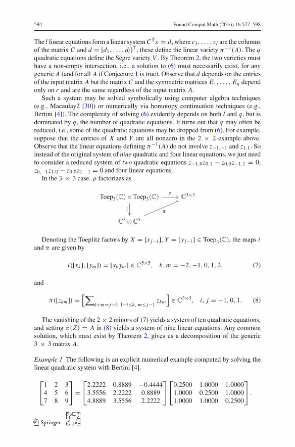
The vanishing of the 2 × 2minors of (7) yields a system of ten quadratic equations,and setting π(Z) = A in (8) yields a system of nine linear equations. Any commonsolution, which must exist by Theorem 2, gives us a decomposition of the generic3 × 3 matrix A.
Example 1 The following is an explicit numerical example computed by solving thelinear quadratic system with Bertini [4].
If we allow 2n Toeplitz matrices T1, . . . , T2n and n permutation matrices P1, . . . , Pn ,then a generic n × n matrix A may be decomposed as
A = T1T2P1T3T4P2 · · · T2n−1T2n Pn . (9)
While this is not strictly speaking a Toeplitz decomposition, it can nonetheless becomputed in polynomial time in exact arithmetic without regard to numerical stability.For a generic matrix A ∈ C
n × n , we may perform Gaussian elimination withoutpivoting to get
A = (I + v1eT1 )(I + v2e
T2 ) · · · (I + vne
Tn ),
where e j is the j th standard basis vector of Cn . If we write I + vkeTk = Πk(I +
wkeT1 )Πk where Πk is the permutation matrix corresponding to the permutation(1 � k) ∈ Sn and wk = Πkvk , then I + wkeT1 = Wk(W
−1k + eneT1 ) where
wk = [wk1, wk2, . . . , wkn]T,
Wk =
⎡⎢⎢⎢⎢⎣
wkn wk,n−1 · · · wk2 wk10 wkn · · · wk3 wk2...
.... . .
......
0 0 · · · wkn wk,n−10 0 · · · 0 wkn
⎤⎥⎥⎥⎥⎦
, eneT1 =
⎡⎢⎢⎢⎢⎣
0 0 · · · 0 00 0 · · · 0 0...
.... . .
......
0 0 · · · 0 01 0 · · · 0 0
⎤⎥⎥⎥⎥⎦
.
Now we may take Tk = Wk and Tk+1 = W−1k + eneT1 to be the required Toeplitz
factors and Pk := ΠkΠk+1 to be the permutation factors, k = 1, . . . , n. The matricesTk and Tk+1 are Toeplitz since Wk is an upper-triangular Toeplitz matrices and theinverse of such a matrix is again an upper-triangular Toeplitz matrix. As the inversionof an upper-triangular Toeplitz matrix requires only O(n log n) arithmetic steps (cfSect. 2), computational cost is at most O(n3), dominated by the arithmetic stepsrequired in Gaussian elimination.
Example 2 Applying the above to a random 5 × 5 matrix with small integer entries
A =
⎡⎢⎢⎢⎢⎣
2 5 2 5 34 5 5 2 22 3 2 1 53 1 5 2 34 1 2 4 3
⎤⎥⎥⎥⎥⎦
,
we obtain A = T1T2P1T3T4P2T5T6P3T7T8P4T9T10P5, where
Here T (v,w) denotes the Toeplitzmatrixwhose first row is v ∈ Cn and first column
is w ∈ Cn .
Acknowledgments We thank Professor T. Y. Lam for inspiring this work. This article is dedicated to his70th birthday. We would also like to thank the anonymous referees for their invaluable comments, particu-larly for the argument after Corollary 1 that substantially simplifies our deduction of Hankel decompositionfrom Toeplitz decomposition. LHL’s work is partially supported by AFOSR FA9550-13-1-0133, NSF DMS1209136, and NSF DMS 1057064. KY’s work is partially supported by NSF DMS 1057064 and NSF CCF1017760.
References
1. “Algorithms for the ages,” Science, 287 (2000), no. 5454, p. 799.2. G. S. Ammar and W. B. Gragg, “Superfast solution of real positive definite Toeplitz systems,” SIAM
J. Matrix Anal. Appl., 9 (1988), no. 1, pp. 61–76.3. Y. Barnea and A. Shalev, “Hausdorff dimension, pro-p groups, and Kac–Moody algebras,” Trans.
Amer. Math. Soc., 349 (1997), no. 12, pp. 5073–5091.4. D. J. Bates, J. D. Hauenstein, A. J. Sommese, and C. W. Wampler, Numerically Solving Polynomial
Systems with Bertini, Software, Environments, and Tools, 25, SIAM, Philadelphia, PA, 2013.5. H. Bart, I. Gohberg, and M. A. Kaashoek, “Wiener-Hopf integral equations, Toeplitz matrices and
linear systems,” pp. 85–135, Operator Theory: Adv. Appl., 4, Birkhäuser, Boston, MA, 1982.6. J. Bernik, R. Drnovšek, D. Kokol Bukovšek, T. Košir, M. Omladic, and H. Radjavi, “On semitransitive
Jordan algebras of matrices,” J. Algebra Appl., 10 (2011), no. 2, pp. 319–333.7. D. Bini and B. Meini, “Solving certain queueing problems modelled by Toeplitz matrices,” Calcolo,
30 (1993), no. 4, pp. 395–420.8. R. B. Bitmead and B. D. O. Anderson, “Asymptotically fast solution of Toeplitz and related systems
of linear equations,” Linear Algebra Appl., 34 (1980), pp. 103–116.9. M. Bordemann, E. Meinrenken, and M. Schlichenmaier, “Toeplitz quantization of Kähler manifolds
and gl(N ), N → ∞ limits,” Comm. Math. Phys., 165 (1994), no. 2, pp. 281–296.10. A. Borel, Linear Algebraic Groups, 2nd Ed., Graduate Texts in Mathematics, 126, Springer-Verlag,
New York, NY, 1991.11. A. Borodin and A. Okounkov, “A Fredholm determinant formula for Toeplitz determinants,” Integral
Equations Operator Theory, 37 (2000), no. 4, pp. 386–396.12. D. Burns and V. Guillemin, “The Tian–Yau–Zelditch theorem and Toeplitz operators,” J. Inst. Math.
Jussieu, 10 (2011), no. 3, pp. 449–461.13. R. H. Chan and X.-Q. Jin, An Introduction to Iterative Toeplitz Solvers, Fundamentals of Algorithms,
5, SIAM, Philadelphia, PA, 2007.14. R. H. Chan and M. K. Ng, “Conjugate gradient methods for Toeplitz systems,” SIAM Rev., 38 (1996),
no. 3, pp. 427–482.
123
Found Comput Math (2016) 16:577–598 597
15. R. H. Chan and G. Strang, “Toeplitz equations by conjugate gradients with circulant preconditioner,”SIAM J. Sci. Statist. Comput., 10 (1989), no. 1, pp. 104–119.
16. T. F. Chan, “An optimal circulant preconditioner for Toeplitz systems,” SIAM J. Sci. Statist. Comput.,9 (1988), no. 4, pp. 766–771.
17. S. Chandrasekaran, M. Gu, X. Sun, J. Xia, and J. Zhu, “A superfast algorithm for Toeplitz systems oflinear equations,” SIAM J. Matrix Anal. Appl., 29 (2007), no. 4, pp. 1247–1266.
18. W. W. Chen, C. M. Hurvich, and Y. Lu, “On the correlation matrix of the discrete Fourier transformand the fast solution of large Toeplitz systems for long-memory time series,” J. Amer. Statist. Assoc.,101 (2006), no. 474, pp. 812–822.
19. W. K. Cochran, R. J. Plemmons, and T. C. Torgersen, “Exploiting Toeplitz structure in atmosphericimage restoration,” pp. 177–189, Structured Matrices in Mathematics, Computer Science, and Engi-neering I, Contemp. Math., 280, AMS, Providence, RI, 2001.
20. F. de Hoog, “A new algorithm for solving Toeplitz systems of equations,” Linear Algebra Appl., 88/89(1987), pp. 123–138.
21. P. Deift, A. Its, and I. Krasovsky, “Asymptotics of Toeplitz, Hankel, and Toeplitz+Hankel determinantswith Fisher–Hartwig singularities,” Ann. Math., 174 (2011), no. 2, pp. 1243–1299.
22. A. Dembo, C. L. Mallows, and L. A. Shepp, “Embedding nonnegative definite Toeplitz matrices innonnegative definite circulantmatrices,with application to covariance estimation,” IEEETrans. Inform.Theory, 35 (1989), no. 6, pp. 1206–1212.
23. R. G. Douglas and R. Howe, “On the C∗-algebra of Toeplitz operators on the quarterplane,” Trans.Amer. Math. Soc., 158 (1971), pp. 203–217.
24. E. Eisenberg, A. Baram, and M. Baer, “Calculation of the density of states using discrete variablerepresentation and Toeplitz matrices,” J. Phys. A, 28 (1995), no. 16, pp. L433–L438.
25. M. Engliš, “Toeplitz operators and group representations,” J. Fourier Anal. Appl., 13 (2007), no. 3, pp.243–265.
27. P. Favati, G. Lotti, and O. Menchi, “A divide and conquer algorithm for the superfast solution ofToeplitz-like systems,” SIAM J. Matrix Anal. Appl., 33 (2012), no. 4, pp. 1039–1056.
28. M. Geck, An Introduction to Algebraic Geometry and Algebraic Groups, Oxford Graduate Texts inMathematics, 10, Oxford University Press, Oxford, 2003.
29. V. Gorin, “The q-Gelfand-Tsetlin graph, Gibbs measures and q-Toeplitz matrices,” Adv. Math., 229(2012), no. 1, pp. 201–266.
30. D. R. Grayson and M. E. Stillman,Macaulay2: A software system for research in algebraic geometry,available at http://www.math.uiuc.edu/Macaulay2/, 2002.
31. U. Grenander and G. Szegö, Toeplitz Forms and Their Applications, 2nd Ed., Chelsea Publishing, NewYork, NY, 1984.
32. J. Haupt,W.U. Bajwa, G. Raz, andR.Nowak, “Toeplitz compressed sensingmatrices with applicationsto sparse channel estimation,” IEEE Trans. Inform. Theory, 56 (2010), no. 11, pp. 5862–5875.
33. R. Howe, “Very basic Lie theory,” Amer. Math. Monthly, 90 (1983), no. 9, pp. 600–623.34. J.-J. Hsue and A. E. Yagle, “Fast algorithms for solving Toeplitz systems of equations using number-
theoretic transforms,” Signal Process., 44 (1995), no. 1, pp. 89–101.35. M. Kac, “Some combinatorial aspects of the theory of Toeplitz matrices,” pp. 199–208, Proc. IBM Sci.
Comput. Sympos. Combinatorial Problems, IBM Data Process. Division, White Plains, NY, 1964.36. H. Khalil, B. Mourrain, and M. Schatzman, “Superfast solution of Toeplitz systems based on syzygy
reduction,” Linear Algebra Appl., 438 (2013), no. 9, pp. 3563–3575.37. A. W. Knapp, Lie Groups Beyond an Introduction, 2nd Ed., Progress in Mathematics, 140, Birkhäuser,
Boston, MA, 2002.38. J. M. Landsberg, Tensors: Geometry and Applications, AMS, Providence, RI, 2012.39. F.-R. Lin, M. K. Ng, and R. H. Chan, “Preconditioners for Wiener-Hopf equations with high-order
quadrature rules,” SIAM J. Numer. Anal., 34 (1997), no. 4, pp. 1418–1431.40. X. Ma and G. Marinescu, “Toeplitz operators on symplectic manifolds,” J. Geom. Anal., 18 (2008),
no. 2, pp. 565–611.41. N. Makarov and A. Poltoratski, “Beurling–Malliavin theory for Toeplitz kernels,” Invent. Math., 180
(2010), no. 3, pp. 443–480.42. R. J. Milgram, “The structure of spaces of Toeplitz matrices,” Topology, 36 (1997), no. 5, pp. 1155–
43. M. K. Ng, Iterative Methods for Toeplitz Systems, Oxford University Press, New York, NY, 2004.44. H. Özbay and A. Tannenbaum, “A skew Toeplitz approach to the H∞ optimal control of multivariable
distributed systems,” SIAM J. Control Optim., 28 (1990), no. 3, pp. 653–670.45. D. Poland, “Toeplitz matrices and random walks with memory,” Phys. A, 223 (1996), no. 1–2, pp.
113–124.46. K. Rietsch, “Totally positive Toeplitz matrices and quantum cohomology of partial flag varieties,” J.
Amer. Math. Soc., 16 (2003), no. 2, pp. 363–392.47. G. W. Stewart, “The decompositional approach to matrix computation,” Comput. Sci. Eng., 2 (2000),
no. 1, pp. 50–59.48. M. Stewart, “A superfast Toeplitz solver with improved numerical stability,” SIAM J. Matrix Anal.
Appl., 25 (2003), no. 3, pp. 669–693.49. J. L. Taylor, Several Complex Variables with Connections to Algebraic Geometry and Lie groups,
Graduate Studies in Mathematics, 46, AMS, Providence, RI, 2002.50. J. Toft, “The Bargmann transform on modulation and Gelfand–Shilov spaces, with applications to
Toeplitz and pseudo-differential operators,” J. Pseudo-Differ. Oper. Appl., 3 (2012), no. 2, pp. 145–227.
51. E. E. Tyrtyshnikov, “Fast computation of Toeplitz forms and somemultidimensional integrals,”RussianJ. Numer. Anal. Math. Modelling, 20 (2005), no. 4, pp. 383–390.
52. S. Serra, “The rate of convergence of Toeplitz based PCGmethods for second order nonlinear boundaryvalue problems,” Numer. Math., 81 (1999), no. 3, pp. 461–495.
53. U. Steimel, “Fast computation of Toeplitz forms under narrowband conditions with applications tostatistical signal processing,” Signal Process., 1 (1979), no. 2, pp. 141–158.
54. G. Strang, “The discrete cosine transform, block Toeplitz matrices, and wavelets,” pp. 517–536,Advances in Computational Mathematics, Lecture Notes in Pure and Applied Mathematics, 202,Dekker, New York, NY, 1999.
55. G. Strang, “A proposal for Toeplitz matrix calculations,” Stud. Appl. Math., 74 (1986), no. 2, pp.171–176.
56. M. Van Barel, G. Heinig, and P. Kravanja, “A stabilized superfast solver for nonsymmetric Toeplitzsystems,” SIAM J. Matrix Anal. Appl., 23 (2001), no. 2, pp. 494–510.
57. K. Ye and L.-H. Lim, “New classes of matrix decompositions,” preprint, (2015).