Evidence for ice flow prior to trough formation in the martian north polarlayered deposits
Dale P. Winebrenner a,b,∗, Michelle R. Koutnik b, Edwin D. Waddington b, Asmin V. Pathare c,d,Bruce C. Murray d, Shane Byrne e, Jonathan L. Bamber f
a Applied Physics Laboratory, Box 355640, University of Washington, Seattle, WA 98195, USAb Department of Earth and Space Sciences, Box 351310, University of Washington, Seattle, WA 98195, USA
c Planetary Science Institute, 1700 E. Ft. Lowell, Suite 106, Tucson, AZ 85719, USAd Division of Geological and Planetary Sciences, California Institute of Technology, Pasadena, CA 91125, USA
e Lunar and Planetary Laboratory, The University of Arizona, Tucson, AZ 85721, USAf Bristol Glaciology Centre, University of Bristol, Bristol BS8 1SS, UK
The north polar layered deposits (NPLD) are the largest sur-face reservoir of martian water ice that actively exchanges withthe atmosphere. Their nearly complete lack of impact craterssuggests that their surface is geologically young, or has been re-cently and extensively modified (Herkenhoff and Plaut, 2000).Alternating bright and dark layers can be seen along the wallsof arcuate troughs that cut through the NPLD. This layered
structure likely reflects deposition during orbitally-driven cli-mate changes (Touma and Wisdom, 1993; Laskar et al., 2002;Levrard et al., 2007), which may have been modified subse-quently, both within and between troughs. Hence, understand-ing the mechanics and evolution of the NPLD is necessary todecipher any evolution of martian climate recorded in the lay-ers.
It is generally assumed that topography and layering of theNPLD are governed by two processes: ice deposition and loss atthe surface (mass balance), and ice flow. However, the relativeimportance of these processes in shaping the NPLD, now or inthe past, remains a fundamental and open question.
Evidence for ice flow prior to trough formation in the martian NPLD 91
To set a framework in which to discuss this question, weintroduce two characteristic time scales. The first is the timerequired to build up an ice sheet through accumulation aloneat some characteristic accumulation rate, or equivalently, to re-move it by ablation alone at some characteristic ablation rate.The second is the time for material to move a characteris-tic distance, such as the length of the ice mass, by flow atsome characteristic speed. The ratio of these two characteris-tic times gives a nondimensional number F , which we call aflow number. In Appendix A, we use conservation laws formass and momentum together with a temperature-dependentconstitutive relation for ice to derive expressions for both ofthese characteristic time scales and for F in terms of char-acteristic values of accumulation rate, temperature, and ice-mass dimensions. When F � 1, mass exchange with the at-mosphere alone controls surface topography, and the ice massis stagnant. When F is of order unity, both surface mass ex-change and ice flow influence the surface shape, and the icemass can be in a near-equilibrium state. When F � 1, iceflow alone controls surface-elevation changes, and surface massexchanges are negligible. On Earth, surging glaciers (Kambet al., 1985) fall in this regime. However, most terrestrialice masses are in a near-equilibrium regime with F of orderunity.
Some researchers have modeled the NPLD as a near-equilibrium regime with F of order unity. Budd et al. (1986)first modeled the NPLD as a large-scale, steady-state flow sys-tem. Zuber et al. (1998) and Zwally et al. (2000) interpretedMars Orbiter Laser Altimeter (MOLA) data from the NPLD assupporting that view. Fisher (1993, 2000) developed a model toexplain more detailed NPLD topography by incorporating flowwith an alternating pattern of accumulation and sublimationresulting from local radiative effects of troughs (i.e., “accubla-tion”). Fisher et al. (2002) found evidence in the directionalityof NPLD surface texture for flow in the directions expectedfrom large-scale topography. Modeling by Hvidberg (2003) andby Pathare and Paige (2005) also supports a role for ice flow inshaping the NPLD, especially near troughs. Nye (2000) evenconsidered martian ice caps shaped entirely by flow in the ab-sence of surface mass fluxes (F � 1).
However, modeled ice flow speeds on Mars are generallyvery slow, even during high obliquity and during NPLD for-mation, so surface mass balance can easily dominate flow inproducing the modeled shape (Greve et al., 2004; Greve andMahajan, 2005). Ivanov and Muhleman (2000), in fact, arguethat the observed NPLD topography can be explained by sub-limation alone. Fishbaugh and Hvidberg (2006) conclude thatinternal layers in the upper portion of the NPLD show no ev-idence of flow, i.e., that the NPLD are currently in a stagnantregime with F � 1.
Thus there is presently no consensus on the roles of surfacemass fluxes and ice flow in shaping the NPLD as a whole. Thissuggests investigation of new alternatives, including a searchfor parts of the NPLD on which effects of relatively recentprocesses may be most evident. Our investigation is motivatedby an examination of MOLA data shaded to emphasize re-gions that are simultaneously high in elevation and low in slope
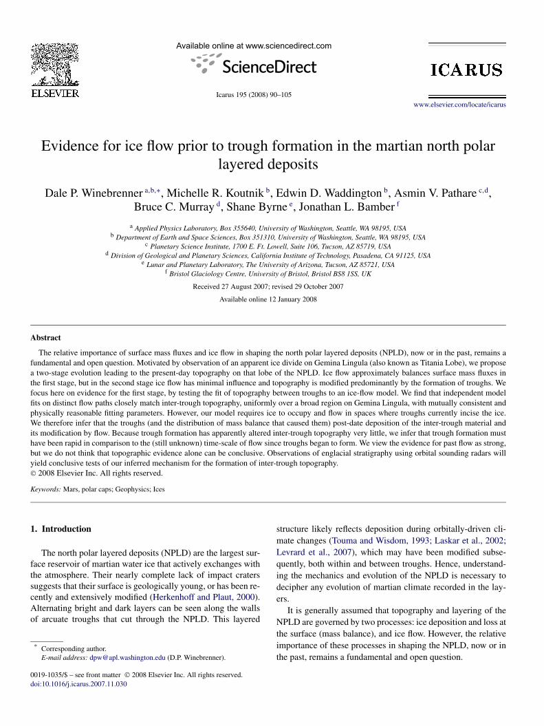
Fig. 1. (a) Digital elevation data for Antarctica, shaded to highlight areas thatare both high in elevation and low in slope (Bamber, 2004). The arrow indi-cates one ice divide among several visible. (b) Digital elevation data from theMOLA laser altimeter for the NPLD. Here we use the 512-point-per-degreeDEM, which does not include data for locations poleward of 87◦ N (Smith etal., 2003). Shading in this presentation is identical to that in (a). Arrows in-dicate a contiguous topographic feature that appears similar to ice divides onEarth.
(Bamber, 2004; Ekholm et al., 1998). On Earth, such shadingeffectively highlights ice divides, which are boundaries sepa-rating regions of flow in different directions. The locations, orabsence, of ice divides are key features on any ice cap. Sur-face slopes on terrestrial ice divides tend to be low and slowlyvarying, and divides tend to be lines with low curvature inmap view. Fig. 1 shows digital elevation models (DEMs) for
92 D.P. Winebrenner et al. / Icarus 195 (2008) 90–105
Antarctica and the NPLD, shaded identically and as describedabove. We focus here on the lobe of the NPLD that boundsChasma Boreale to the south and east, which has recentlybeen named Gemina Lingula by the International AstronomicalUnion. Here we refer to this feature as Titania Lobe (Pathareand Paige, 2005). A ridge running along the lobe resembles icedivides on both Antarctica and Greenland (Ekholm et al., 1998;Bamber, 2004).
While resemblance does not establish analogous ice dynam-ics on Earth and Mars, it does suggest quantitative tests basedon topography. The relative lack of troughs cutting the candi-date divide suggests to us that present-day topography betweentroughs may preserve evidence of ice flow in a previous era.The layering observed along PLD trough walls also clearly in-dicates that troughs formed after the inter-trough topography bycutting into pre-existing ice (Cutts, 1973; Howard et al., 1982;Thomas et al., 1992).
We therefore consider a new approach to the question ofwhether ice flow has influenced NPLD structure, at least on Ti-tania Lobe. Rather than trying to explain topography on thislobe with one set of processes acting at all times (with orwithout flow), we propose a two-stage evolution leading to thepresent-day NPLD. Ice flow and surface mass exchanges wereapproximately balanced in the first stage (i.e., F ∼1), but a sec-ond stage followed and continues up to the present in whichF � 1; ice flow has had minimal influence in this second stageand topography has been modified predominately by the forma-tion of troughs.
We begin testing this scenario by ignoring the troughs (fornow), and testing current topography on Titania Lobe, betweenthe troughs (cf. Section 2.1, Fig. 4) for evidence that the firststage of evolution actually occurred. Specifically, we solve anice-flow inverse problem by fitting an ice-flow model to ob-servations, thus estimating mass balance and flow parameterswithin the model scenario. (This stands in contrast to solu-tion of a forward problem, in which parameters and forcing areprescribed and the ice-flow model predicts observables.) Expe-rience with analogous inverse problems on terrestrial ice caps(Waddington et al., 2007; see also Section 4) indicates that ifno flow has occurred, solutions of the inverse problem will fitobserved topography poorly, or solutions on distinct parts ofthe topography will yield inconsistent and unphysical parame-ter inferences. Solutions that agree with the actual topography,using mutually consistent and physically reasonable parame-ters, would be evidence that a balance between mass fluxes andflow did in fact govern formation of the topography betweentroughs.
We find that independent model fits on distinct flow pathsin fact closely match inter-trough topography, uniformly overa broad region on Titania Lobe. The parameters inferred fromdistinct fits are mutually consistent across the region. The previ-ous ice extent inferred from fitted parameters closely tracks thepresent margin of the lobe, except in part of Chasma Boreale(where it diverges plausibly). The inferred pattern of mass bal-ance is plausible, and the inferred ice-flow law coincides withthat commonly found in flowing ice masses on Earth.
While we do not think that topographic evidence alone canbe conclusive, we interpret our results as strong evidence forthe occurrence of the first stage in our scenario.
In that first stage, however, ice would have occupied andflowed in spaces where troughs currently incise Titania Lobe.We therefore infer that the troughs post-date deposition of theinter-trough material and its modification by flow—i.e., theconsistency of fits is evidence that the second stage of our sce-nario also occurred (though we do not attempt to model thatsecond stage here). Because our assumed spatial distributionof mass balance differs strongly from that necessary to ex-plain troughs, we also infer a fundamental change in the mass-balance distribution on Titania Lobe. Finally, because troughformation has apparently altered inter-trough topography verylittle, we infer that trough formation must have been rapidin comparison to the (still unknown) time-scale of flow sincetroughs began to form.
This remainder of this paper is organized as follows: Be-cause the particular methods employed here are not explicitin literature on terrestrial ice masses, we present our methodsin Section 2, with details in Appendix A. Section 3 presentsnumerical results of our analysis on individual topographic pro-files as well as the statistics of parameters inferred from 40profiles covering a broad swath on Titania Lobe. We discussinterpretation of the numerical results in Section 4. Section 5presents conclusions and our views on further work, partic-ularly with regard to radar-observed stratigraphy within theNPLD which could conclusively test our inferences, and couldyield more detailed information on past and present flow dy-namics and mass balance.
2. Methods
Throughout this work, we use the 512-point-per-degree(ppd), polar-stereographic projection of the MOLA DEM ofthe NPLD, which is composed of square pixels measuring ap-proximately 115.09 m on a side (Smith et al., 2003).
The geometrical specification of our problem requires an as-sumption for the basal topography beneath Titania Lobe. Weassume that topography is constant in elevation at −5100 mrelative to the martian geoid, consistent with the exceptionalflatness of surrounding topography and with a recent radar ob-servation showing no evidence for lithospheric deflection be-neath the NPLD near Titania Lobe (Picardi et al., 2005).
Our methods then divide naturally into two parts: (1) opera-tions on the MOLA DEM to specify surface elevation data foruse in an ice-flow inverse problem; and (2) specification andsolution of the inverse problem.
2.1. Delineation of inter-trough topography, candidate flowlines and flow bands
To compare MOLA data with an ice-flow model, we mustfirst delineate objectively topography that would preserve infor-mation about flow. According to our hypothesis, this is topog-raphy between troughs. Topography on Titania Lobe outsideof troughs generally has small slopes compared to slopes on
Evidence for ice flow prior to trough formation in the martian NPLD 93
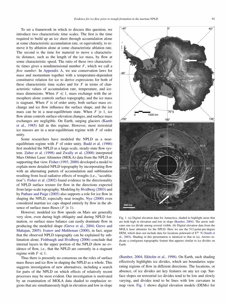
Fig. 2. Elevation contours with 300 m spacing on the MOLA DEM (red) and on the interpolated, smoothed surface derived from inter-trough topography (yellow).The underlying shaded-relief is the MOLA DEM (with shading identical to that in Fig. 1b) restricted to inter-trough topography as delineated by our procedure.Gradient paths orthogonal to the yellow contours thus coincide with prospective ice flow paths on inter-trough topography, and they traverse troughs on paths thatice flow would have taken prior to trough formation (i.e., at a previous time when the now-empty troughs were filled with ice).
trough walls. Empirically, we find that topography with eleva-tion gradients less than 0.015 rad (0.86◦) in magnitude coin-cides with inter-trough topography as determined by inspec-tion, except in small areas at the bottoms of troughs wherethe dominant slopes change sign. After removal of such ar-eas, the remaining low-slope DEM pixels constitute our esti-mate of inter-trough topography. (For quantitative details seeAppendix A.)
Next, we identify prospective flow lines as elevation gra-dients on a smooth surface that we derive from inter-troughtopography by bridging the troughs across their tops andsmoothing the result. Elevation contours on the interpolated,smoothed surface closely match those of the original MOLAdata for locations on the inter-trough topography (Fig. 2). Gra-dient lines on the smoothed surface therefore coincide withthose derived purely from MOLA data on inter-trough topog-raphy, but span the troughs on paths that ice flow would take,were the troughs filled with ice.
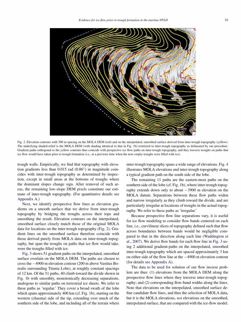
Fig. 3 shows 51 gradient paths on the interpolated, smoothedsurface overlain on the MOLA DEM. The paths are chosen tocross the −4900 m elevation contour (200 m above Vastitas Bo-realis surrounding Titania Lobe), at roughly constant spacingsof 12 km. Of the 51 paths, 40 climb toward the divide shown inFig. 1b with smoothly, monotonically decreasing separations,analogous to similar paths on terrestrial ice sheets. We refer tothese paths as ‘regular.’ They cover a broad swath of the lobewhich spans approximately 400 km (cf. Fig. 1b), starting on thewestern (chasma) side of the tip, extending over much of thesouthern side of the lobe, and including all of the terrain where
inter-trough topography spans a wide range of elevations. Fig. 4illustrates MOLA elevations and inter-trough topography alonga typical gradient path on the south side of the lobe.
The remaining 11 paths are the eastern-most paths on thesouthern side of the lobe (cf. Fig. 1b), where inter-trough topog-raphy extends down only to about −3900 m elevation on theMOLA datum. Separations between these flow paths widenand narrow irregularly as they climb toward the divide, and areparticularly irregular at locations of troughs in the actual topog-raphy. We refer to these paths as ‘irregular.’
Because prospective flow line separations vary, it is usefulfor ice flow modeling to consider flow bands centered on eachline, i.e., curvilinear slices of topography defined such that flowacross boundaries between bands would be negligible com-pared to that in the direction along each line (Waddington etal., 2007). We derive flow bands for each flow line in Fig. 3 us-ing 2 additional gradient-paths on the interpolated, smoothedinter-trough topography which are spaced approximately 3 kmon either side of the flow line at the −4900 m elevation contour(for details see Appendix A).
The data to be used for solution of our flow inverse prob-lem are thus: (1) elevations from the MOLA DEM along theprospective flow lines where they traverse inter-trough topog-raphy; and (2) corresponding flow-band widths along the lines.Note that elevations on the interpolated, smoothed surface de-fine candidate flow lines, and thus the selection of MOLA data,but it is the MOLA elevations, not elevations on the smoothed,interpolated surface, that are compared with the ice-flow model.
94 D.P. Winebrenner et al. / Icarus 195 (2008) 90–105
Fig. 3. Paths along elevation gradients on the smoothed, interpolated surface derived from inter-trough topography, superimposed on the MOLA DEM of TitaniaLobe. Two elevation contours are also shown, the lower at −4900 m (200 m above the part of Vastitas Borealis surrounding Titania Lobe) and the higher at −3900 m.Eleven of the paths (shown in blue) are ‘irregular,’ as defined in the text. The remaining 40 (shown in red and white) are ‘regular’; these paths constitute our estimatesof ice flow lines, if and when ice actually did flow on Titania Lobe. (We number the regular, paths starting with the westernmost path on the side of the tip in ChasmaBoreale, for reference. Paths 1, 11, 21, and 31 are shown in white for reference.) We use the pixel locations that constitute regular paths to select elevation data fromthe MOLA DEM for comparison with an ice-flow model. Elevations from the smoothed, interpolated surface are not compared with the model.
2.2. Specification and solution of an ice-flow inverse problem
Next, we specify a model for the topography of a flow-ing ice mass with a parameterized distribution of surface massfluxes. Large-scale topography is more sensitive to ice dynam-ics than to the spatial distribution of surface mass balance, andthus by itself can yield information only on the gross patternof balance (Paterson, 1994). Even the gross mass-flux patternon the surface of Titania Lobe is highly uncertain (observa-tions are lacking and mechanisms responsible for the balanceare poorly known). However, the overall shape of inter-troughtopography—decreasing slope with increasing elevation—andthe position of the apparent ice divide suggest to us a patternof accumulation at higher elevations and ablation (via sublima-tion) at lower elevations at the time when inter-trough topogra-phy formed. Such a pattern would be somewhat similar to thatproposed by Fisher (1993), who argued that the presence of asecond spreading center in Titania Lobe distinct from the maincap could explain the overall spiral pattern of troughs on theNPLD.
Thus, without speculating on what physics would producesuch an Earth-like pattern on Mars, we assume a steady-statesurface mass balance rate (units ice volume area−1 time−1) withuniform (spatially constant) accumulation along a given flowline, starting at the ice divide and extending downhill to anequilibrium-line location, which is to be determined by themodel fit. Mass balance at the equilibrium line changes dis-continuously from accumulation to ablation. We then assume
a uniform ablation rate between the equilibrium line locationand the terminus of the flow line (see Fig. 4b). The assumptionof a steady state implies that the equilibrium-line location de-pends only on the geometry of the flow band and on the ratioof accumulation and ablation rates, rather than on their absolutevalues.
Maintenance of steady-state topography requires ice to flowfrom regions of accumulation to regions of ablation. (A quanti-tative version of this requirement is given in Appendix A.) Weassume that the ice in Titania Lobe is, and has always been,frozen to its bed, so that there is no mass flux across its lowerboundary. Then at each point, P , along the flow line, the massflux due to flow through a vertical cross-section of the flow bandmust balance the surface mass flux into the band integratedfrom P up to the ice divide (where the flow-band width, andtherefore surface mass flux into the band, decreases to zero).We link this kinematic balance to the surface slope at P byassuming that the driving stress is determined solely by the sur-face slope and ice thickness at P , and that there is no slidingat the bed (consistent with the frozen-bed assumption). We ex-press the mass flux through the flow-band cross section in termsof a depth-averaged velocity. The latter can be derived from theassumptions on driving stress and bed elevations, together witha flow law to relate strain rate to stress in the ice. We assume apower-law form for the flow law, with exponent n (Glen, 1955;Goldsby and Kohlstedt, 2001), which we take as a parameter.We take the temperature-dependent factor in the flow law, andthus temperature, to be constant over depth and over the flow
Evidence for ice flow prior to trough formation in the martian NPLD 95
Fig. 4. (a) MOLA elevation data along regular gradient path 29, on the southside of Titania Lobe, with elevations given as meters above −5100 m. Eleva-tions located on inter-trough topography, as shown in Fig. 2, are denoted byheavy black lines. (b) A generic example of the spatial pattern of surface massbalance rate (units ice volume area−1 time−1) along the gradient path, as as-sumed in our model (cf. Section 2.2). The mass balance is positive (onto theice mass) and uniform (spatially constant) from the ice divide to an equilib-rium-line location, which is to be determined by model fitting. Mass balanceat the equilibrium line changes discontinuously from positive (accumulation)to negative (ablation due to sublimation). The ablation rate is then uniformbetween the equilibrium-line location and the terminus of the flow line. Ourmodel fits determine only relative magnitudes of accumulation and ablation(cf. Section 2.2 and Appendix A)—hence rates in this plot are relative ratherthan absolute, and would be multiplied by the ablation rate (were it known) toobtain absolute rates.
lines. Integration of surface slope along the flow line then yieldsthe surface-elevation profile. We give a mathematical formula-tion of this model in Appendix A. Our model is, however, onlya slight generalization of that given by Paterson (1972), and itreduces to that model for a flow band of uniform width.
As in Paterson’s model, the equilibrium-line position setsthe spatial pattern of ice velocities, but not their absolutemagnitudes—the steady-state condition equally allows slowflow with small surface fluxes, or faster flow with larger fluxes.The model fits shown below therefore provide no informa-tion on rates at the time that inter-trough topography formed.Our model does, however, couple ice temperature near the bed(where most strain occurs) to flow speeds and absolute massflux rates. Thus a combination of this work with englacial tem-perature modeling (e.g., through obliquity cycles) will provideestimates of absolute rates and characteristic time-scales for theformation of inter-trough topography by flow. We discuss suchfuture work in the final section of this paper, but our aim here isfirst to address the question of whether inter-trough topographyin fact preserves evidence of flow.
The final element of our method is a particular algorithm tosolve the inverse problem. Note that all topographies that can be
generated by our model vary slowly on the scale of the ice thick-ness. We seek to interpret the large-scale topography of TitaniaLobe, rather than the fine-scale topography observed betweentroughs (which is presumably due to more complex patternsof mass balance, or perhaps bed topography, than can be di-agnosed from surface topography alone). The smoothness ofall model topographies relative to the data, and the small num-ber of model parameters relative to independent data points,prevents over-fitting; thus constraining fits (using, for example,Lagrange multipliers) proves to be unnecessary. Moreover, forthis initial work, we seek a very straightforward inverse method,even at the cost of quantitative information on uncertainties inour fitted parameters (i.e., resolving power).
We therefore fit our model to inter-trough topography sim-ply by minimizing the mismatch between model and data, in theleast-squares sense, as we vary 4 model parameters: (1) the icethickness, H , at the highest point on the flow line, i.e., wherethe flow band width decreases to zero on the ice divide; (2) theextent, L, of the model topography along the flow line; (3) theposition of the equilibrium line along the flow line; and (4) theflow-law exponent, n. We fit the model on each flow line inde-pendently of fits along any other flow lines, so each fit yieldsindependent parameter estimates. Consistency between para-meter estimates from distinct flow lines indicates consistencyin the physics contained in the model and the topography at dif-ferent locations on Titania Lobe.
3. Results
On 39 of the 40 regular paths (cf. Section 2.1), the ice-flowmodel fits the observed inter-trough topography to within aroot-mean-square (RMS) mismatch of 10–26 m, which is 1–2% of the range of inter-trough topography elevations along theflow lines. The remaining path, on which the RMS mismatch is32 m, is the path most closely neighboring the irregular paths(path 40). We show below that these fitted model topographies,i.e., fits, closely track both the elevations and slopes of inter-trough topography over the entire region of regular paths. Thequestion is therefore whether the inferred model parameters areconsistent and physically reasonable.
Because topography is more sensitive to flow dynamics thanto the spatial pattern of mass balance, consider first consistencywith respect to the ice flow-law exponent, n. Fig. 5 shows his-tograms of the RMS mismatches for several values of n. Thevalue n = 1 corresponds to linear, viscous (Newtonian) flow,such as may occur in ice at very low strain rates (e.g., Pettitand Waddington, 2003). The value n = 1.8 occurs for ice withgrain sizes on the order of microns and under cold conditions(Goldsby and Kohlstedt, 2001), and thus might be expected toapply on Mars (Pathare and Paige, 2005). Values of n = 3 to4 are characteristic of ice flow on Earth at relatively high strainrates, with grain sizes on the order of millimeters and basal tem-peratures greater than about −12 ◦C, while n = 6 approximatesthe flow law for perfectly plastic material (Paterson, 1994).
Perhaps surprisingly, fits with the smaller exponents yieldconsiderably poorer fits than those obtained with n = 3 andn = 4—the distributions of best-fit RMS mismatches for n =
96 D.P. Winebrenner et al. / Icarus 195 (2008) 90–105
Fig. 5. Histograms of RMS mismatches between the MOLA DEM on inter-trough topography and best-fit model elevations, on the 40 flow lines shown in red inFig. 3, for 5 values of the flow-law exponent, n. Relative frequencies sum to 1, and the dashed and solid lines indicate the median and mean values, respectively, foreach value of n. RMS mismatches are smallest, and the distributions most compact, for n = 3 and n = 4, with little to distinguish distributions for those values of n.Larger values of n yield the lowest values of RMS mismatch in some cases, but are generally not optimal and yield larger numbers of large RMS mismatches thando n = 3 and n = 4.
3–4 have the smallest means and nearly the smallest medians.They include the smallest mismatches observed for any valuesof n, and they include the fewest large mismatches in any ofthe distributions. Fits with n = 6 yield the lowest median RMSmismatch, but also yield more large mismatches than those withn = 3–4. We show below that those profiles that are fit well withn = 6 may yield some additional insight. However, flow-law ex-ponents of 3–4 clearly yield excellent fits to all of the 40 regularprofiles and are the best values overall for fitting that set.
Inspection of individual fits shows that the fits are accuratenot only statistically, but also point by point along each profile.The flow-line elevations in Fig. 6a are from the southern sideof Titania Lobe, where inter-trough topography occurs over abroad range of elevations. The flow line is one of the regularpaths, and the fit is representative of those from the southernside of the lobe. In this case, the best-fit profile with n = 3 fitsthe data slightly better than that with n = 4 (RMS mismatchesof 10.5 m vs 12.7 m), but both fits follow the actual shape ofinter-trough topography very closely. Estimates of equilibrium-line positions differ somewhat between values of n, but thedifference is similar to the widths of the minima in RMS mis-matches between model and data (Fig. 6b).
By contrast, our model fails to fit accurately the elevationsalong paths on parts of Titania Lobe with (apparently) little re-maining inter-trough topography, as shown in Fig. 7. The flowline in Fig. 7 is one of the 11 irregular lines, along which most
inter-trough topography is confined to high elevations. RMSmismatches for this and neighboring flow lines exceed 44 m(and are not included in the histograms in Fig. 5). Moreover,modeled and observed topographies differ even qualitatively(except at the highest elevations). Thus consistency between re-sults on various paths is not somehow inherent in our model, butrather indicates a physically consistent explanation in those lo-cations where it occurs.
Fig. 8 shows fits from a spatially extensive sample from the40 regular profiles in Fig. 3, spanning the area from the tip ofTitania Lobe around to the region of irregular profiles. Fits inall of these cases, as well as that shown in Fig. 10 and the 30remaining regular cases not plotted here, are much more similarto those in Fig. 6 than to those in Fig. 7—fits with flow-lawexponents of 3 and 4 closely track inter-trough topography from400 m to 1900 m above Vastitas Borealis (i.e., from −4700 to−3200 m).
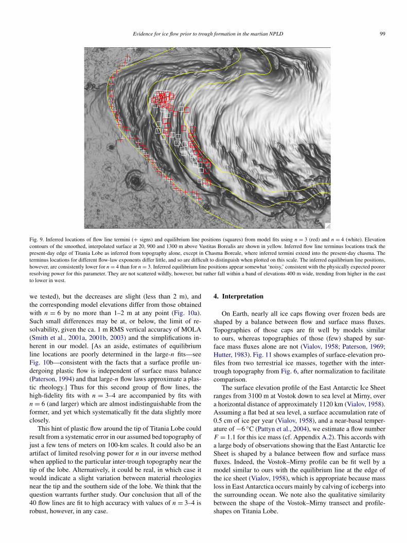
There is also consistency between the other model parame-ters inferred from individual flow lines. Fig. 9 shows for all40 profiles the inferred termini of the flow lines, i.e., the in-ferred extent of the ice cap at the time of flow; results for fitswith n = 3 and n = 4 are shown in red and white, respectively.Estimates of terminus positions are tightly determined by thefits and differ little for the two flow law exponents. They aremutually consistent between independent flow lines, and more-over they track the present-day extent of Titania Lobe closely
Evidence for ice flow prior to trough formation in the martian NPLD 97
Fig. 6. (a) Representative data and model fits from path 29, on the southernside of Titania Lingula away from the tip. MOLA data along the flow line areshown by the thin black line, with elevations given as meters above −5100 m.Inter-trough topography is shown by the thick black line. (The data and flow linefor this figure are identical to those in Fig. 4.) The dashed curve is the result ofminimizing the RMS mismatch between inter-trough elevations and the modelover all values of H , L, and equilibrium position, R, while holding the flow-lawexponent, n equal to 3. The estimated position of the equilibrium line is markedby the dashed vertical line. The minimized RMS mismatch is 10.5 m. Dottedlines show the corresponding fit and estimate of equilibrium line position withn = 4, for which the RMS mismatch is 12.7 m The fit with n = 4 is difficultto distinguish from that with n = 3 at this scale. (b) Plots of RMS mismatchesbetween inter-trough elevations and fits as position of the equilibrium line isallowed to vary (and best-fit values H and L are chosen separately for eachequilibrium line position). Mismatches for fixed n = 3 and n = 4 are plotted asdashed and dotted lines, respectively.
(though flow lines terminating in Chasma Boreale suggest anearlier extension of the ice into that feature). Our procedure in-fers the ice thickness at the divide (i.e., at the head of the flowband) as well. The inferences are strongly constrained by ourassumption for basal topography and the MOLA-observed ele-vations on the divide. They therefore closely and consistentlytrack the divide elevations, though mainly by virtue of theirstrong constraint by the data.
The fourth and final set of inferred parameters are the po-sitions of equilibrium lines. The solution of our inverse prob-lem yields the least resolution for those positions (cf. Figs. 6band 10b), consistent with the relative insensitivity of topogra-phy to mass-balance distributions. Equilibrium-line positionsfrom fits with n = 3 (in red) and n = 4 (in white) in Fig. 9 dis-play some pseudo-random variability, and fits with the largerexponent yield slightly lower-elevation positions. All of the es-
Fig. 7. Data and model fits from one of the flow lines that converge irregularlytoward the divide on the southern side of Titania Lingula (cf. Fig. 3—this pathis number 42 if we extend the numbering of regular paths into the irregularpaths). Fits are for flow law exponents n = 3 (dashed, RMS mismatch betweenmodel and data of 44.5 m) and n = 4 (dotted, 51.6 m RMS mismatch). The fitshere are not only quantitatively less accurate than those in Fig. 6, but also differqualitatively in shape from the data.
timates, however, lie between −3900 and −4300 m, generallytrending from higher in the east to lower in the west. Sucha trend could plausibly result from atmospheric (or perhapsradiation-driven) processes, and certainly stands in contrast touncorrelated variations over a large region on the lobe. Theinferred equilibrium-line positions therefore also appear to beconsistent, within the apparent limits on our resolving powerfor that variable.
Thus, the high-fidelity model fits to inter-trough topography,on 40 independent profiles covering a broad area on TitaniaLobe, are obtained with mutually consistent values for all in-ferred parameters. This is our primary result.
There may, in addition, be some insight available from aslight, but systematic, difference in fits on different parts ofthe lobe. Specifically, the 40 regular flow lines divide into twospatially contiguous groups, distinguished by the behavior ofRMS mismatches of fits versus n: (1) a group of 22 lines onthe southern side of the lobe, which starts at the boundary withthe irregular lines and extends westward toward (but does notreach) the tip of the lobe; and (2) a group of 18 lines, which cov-ers the tip of the lobe on both its northern and southern sides. Inthe first group, the RMS mismatches of fits attain their globalminima for values of n = 3–4; RMS mismatches of the bestpossible fits holding n = 6 exceed those with n = 3–4 by a fewmeters up to a maximum of 13 m. Thus fits on the southern sideof Titania Lobe clearly favor flow-law exponents in the range3–4 over all other flow law exponents tested.
Fits in the second group with n = 3 to 4 also track inter-trough topography very closely (see Figs. 8 and 10), withRMS mismatches in the range 20–26 m. Fits with n = 6 inthis group, however, yield model elevations which differ byno more than a few meters, anywhere along the flow line,from those obtained with n = 3–4. The minimum RMS mis-matches with n = 6 are 0–3.5 m lower those for n = 4. Infact, minimum RMS mismatches decrease yet further with in-creasing n, up to at least n = 7.5 (the largest value of n that
98 D.P. Winebrenner et al. / Icarus 195 (2008) 90–105
Fig. 8. Eight additional representative topographic profiles and model fits analogous to those in Figs. 6 and 7. (Left to right, and row by row starting at the top, thesequence of path numbers is 3, 12, 18, 26, 30, 31, 33, 39—cf. Fig. 3.) Fits using n = 3 are again denoted by dashed lines, and fits n = 4 are denoted by dotted lines.The quality of fits is very similar to that observed on the other 30 regular profiles that are not shown in this paper. In most cases, it is difficult to distinguish the fitsvisually on the scale plotted here—the primary differences are in the inferred positions of equilibrium lines.
Evidence for ice flow prior to trough formation in the martian NPLD 99
Fig. 9. Inferred locations of flow line termini (+ signs) and equilibrium line positions (squares) from model fits using n = 3 (red) and n = 4 (white). Elevationcontours of the smoothed, interpolated surface at 20, 900 and 1300 m above Vastitas Borealis are shown in yellow. Inferred flow line terminus locations track thepresent-day edge of Titania Lobe as inferred from topography alone, except in Chasma Boreale, where inferred termini extend into the present-day chasma. Theterminus locations for different flow-law exponents differ little, and so are difficult to distinguish when plotted on this scale. The inferred equilibrium line positions,however, are consistently lower for n = 4 than for n = 3. Inferred equilibrium line positions appear somewhat ‘noisy,’ consistent with the physically expected poorerresolving power for this parameter. They are not scattered wildly, however, but rather fall within a band of elevations 400 m wide, trending from higher in the eastto lower in west.
we tested), but the decreases are slight (less than 2 m), andthe corresponding model elevations differ from those obtainedwith n = 6 by no more than 1–2 m at any point (Fig. 10a).Such small differences may be at, or below, the limit of re-solvability, given the ca. 1 m RMS vertical accuracy of MOLA(Smith et al., 2001a, 2001b, 2003) and the simplifications in-herent in our model. [As an aside, estimates of equilibriumline locations are poorly determined in the large-n fits—seeFig. 10b—consistent with the facts that a surface profile un-dergoing plastic flow is independent of surface mass balance(Paterson, 1994) and that large-n flow laws approximate a plas-tic rheology.] Thus for this second group of flow lines, thehigh-fidelity fits with n = 3–4 are accompanied by fits withn = 6 (and larger) which are almost indistinguishable from theformer, and yet which systematically fit the data slightly moreclosely.
This hint of plastic flow around the tip of Titania Lobe couldresult from a systematic error in our assumed bed topography ofjust a few tens of meters on 100-km scales. It could also be anartifact of limited resolving power for n in our inverse methodwhen applied to the particular inter-trough topography near thetip of the lobe. Alternatively, it could be real, in which case itwould indicate a slight variation between material rheologiesnear the tip and the southern side of the lobe. We think that thequestion warrants further study. Our conclusion that all of the40 flow lines are fit to high accuracy with values of n = 3–4 isrobust, however, in any case.
4. Interpretation
On Earth, nearly all ice caps flowing over frozen beds areshaped by a balance between flow and surface mass fluxes.Topographies of those caps are fit well by models similarto ours, whereas topographies of those (few) shaped by sur-face mass fluxes alone are not (Vialov, 1958; Paterson, 1969;Hutter, 1983). Fig. 11 shows examples of surface-elevation pro-files from two terrestrial ice masses, together with the inter-trough topography from Fig. 6, after normalization to facilitatecomparison.
The surface elevation profile of the East Antarctic Ice Sheetranges from 3100 m at Vostok down to sea level at Mirny, overa horizontal distance of approximately 1120 km (Vialov, 1958).Assuming a flat bed at sea level, a surface accumulation rate of0.5 cm of ice per year (Vialov, 1958), and a near-basal temper-ature of −6 ◦C (Pattyn et al., 2004), we estimate a flow numberF = 1.1 for this ice mass (cf. Appendix A.2). This accords witha large body of observations showing that the East Antarctic IceSheet is shaped by a balance between flow and surface massfluxes. Indeed, the Vostok–Mirny profile can be fit well by amodel similar to ours with the equilibrium line at the edge ofthe ice sheet (Vialov, 1958), which is appropriate because massloss in East Antarctica occurs mainly by calving of icebergs intothe surrounding ocean. We note also the qualitative similaritybetween the shape of the Vostok–Mirny transect and profile-shapes on Titania Lobe.
100 D.P. Winebrenner et al. / Icarus 195 (2008) 90–105
Fig. 10. (a) Representative data and model fits from path 4, on the tip of Tita-nia Lobe, for flow law exponents n = 3 (dashed line, RMS difference betweenmodel and data of 25.9 m), n = 4 (solid line, 22.4 m RMS difference), andn = 6 (dotted line, 19.0 m RMS difference). (b) Plots of RMS differences forn = 3 (dashed line), n = 4 (solid line), and n = 6 (dotted line) vs equilibriumline position, as in Fig. 6b. Inferred positions of the equilibrium line differ lit-tle between fits with n = 3 and n = 4 in this case (and generally near the tip ofthe lobe, cf. Fig. 8), but the minima in RMS differences are broader than thosefor profiles on the southern side of the lobe. The minimum in RMS differencefor n = 6 is very broad, suggesting that the profile is nearly independent of sur-face mass balance. Such independence would be consistent with a plastic flowlaw, in which n approaches infinity (Paterson, 1994).
By contrast, the shape of the Meighen Ice Cap in the Cana-dian Arctic differs qualitatively from any that we observe onTitania Lobe. The shape of Meighen Ice Cap is controlled bysurface mass fluxes rather than by flow (Hutter, 1983). Thisis in accord with our estimate of F = 0.01 for this ice cap,based on dimensions reported by Paterson (1969), a surface ab-lation rate of 0.1 m per year (Koerner, 2005), and an assumednear-basal temperature of −5 ◦C. It is also consistent with theinability of our ice-flow model to fit the Meighen thickness pro-file accurately—the slopes of all model profiles are largest nearthe terminus and decrease monotonically with increasing icethickness toward the divide, whereas the slope of the Meighenthickness profile is maximum at intermediate thicknesses. Con-versely, there is no known ice mass on Earth whose shape isdominated by surface mass fluxes but which mimics the shapeof ice masses that are shaped by balance between flow and sur-face mass fluxes.
Likewise on Titania Lobe, we consider it implausible to pos-tulate ad hoc variations of surface mass fluxes (in space andtime) so as to yield current topography that mimics that shaped
Fig. 11. Profiles of normalized ice thickness versus normalized horizontal dis-tance for the Meighen Ice Cap in the Canadian Arctic (1), the East Antarctic IceSheet between Vostok and Mirny Stations (+), and Titania Lobe (specifically,the profile shown in Fig. 6, denoted by solid black lines). The normalization forice thickness is the maximum ice thickness on the profile (for each profile sep-arately). The normalization for horizontal distance is the length of the profile.The Meighen Ice Cap is the smallest of the three, with a maximum thicknessof 85 m and extent of 2.5 km. The Vostok–Mirny traverse attains a thicknessof 3100 m near Vostok and extends 1122 km. The data from Titania Lobe havebeen normalized by the thickness at the divide (1900 m) and extent of the flowline (320 km) inferred from the best fit of our ice-flow model to inter-troughtopography using flow-law parameter n = 3 (using n = 4 yields a nearly iden-tical plot). The dashed lines show the best fit model profile for n = 3 in thecase of Titania Lobe, and the model of Vialov (1958) in the case of the EastAntarctic data.
by balance between flow and surface fluxes—and moreoverdoes so only for topography between troughs. We thereforeknow of no physical mechanism other than flow that couldproduce the inter-trough topography on Titania Lobe so consis-tently. We interpret the consistency and fidelity of fits on widelyseparated profiles as evidence that our ice-flow model capturesthe essential physics responsible for the topography.
Our interpretation requires, however, that the troughs wereoccupied by flowing ice at the time that the inter-trough topog-raphy formed. We infer that the troughs must post-date theinter-trough topography, which in turn requires a significantchange in the distribution, and perhaps magnitude, of surfacemass balances on Titania Lobe.
The ice-flow model fits inter-trough topography closely overnearly the full range of elevation (cf. Figs. 6, 8, 10, and 11).This indicates that troughs have incised the prior surface sorapidly, compared to the time-scale of ice flow during troughformation, that the record preserved in the inter-trough topogra-phy remained nearly undisturbed. Neither has flow subsequentto trough formation had sufficient time to deform inter-troughtopography very much, either because flow has been slow, ortime has been short, or both.
5. Conclusions
We have presented strong evidence that ice flow has shapedthe topography of the NPLD, at least on Titania Lobe, duringsome time in the past. We derive the evidence for flow frominter-trough topography that (we infer) survives from a previ-ous era. Inspection of Fig. 1b suggests that much less ‘relict’
Evidence for ice flow prior to trough formation in the martian NPLD 101
topography survives elsewhere on the NPLD, and thus that Ti-tania Lobe may have been glaciologically active more recentlythan other regions of the NPLD, or that ‘relict’ topographyhas been better preserved there. Either of these conclusions, ifconfirmed, would have broad and significant implications forwhere to seek, and how to analyze, martian climate records pre-served in the NPLD. We therefore regard not merely strong, butconclusive tests of our scenario to be a priority for our futurework.
Recent and continuing observations of internal stratigraphyin the NPLD using radar (Picardi et al., 2005; Phillips et al.,2007; Holt et al., 2007) will allow conclusive tests of our sce-nario. In particular, internal layers in our scenario must in-tersect the (inter-trough) surface of the ice at all elevationsin the inferred ablation zone, whereas layers in the accumu-lation zone can never intersect the ice surface (Fisher, 2000;Siegert and Fisher, 2002; Koutnik et al., 2006).
If our scenario survives conclusive testing, a key questionwould clearly be when the inferred change in the mass bal-ance regime occurred. Because our model fits imply no ab-solute time scale, we cannot yet constrain the timing of thechange in mass balance regime or the age of the inter-troughsurface. The path toward such constraint is clear, however, andit again involves radar stratigraphic observations. During thepostulated era of flow, internal layers shaped by deposition andflow would have extended unbroken across spaces now occu-pied by troughs. Later alteration of the surface by trough for-mation must have resulted in new stresses that strained ice, andso deformed layers, in the vicinity of trough walls. The spatialextent and shape of layer deformation would depend on the sur-face temperature history and time over which the new stresseshave acted. Thus radar observations of layering near troughs,in combination with flow modeling under current and recentlypast temperature-conditions (cf. Pathare and Paige, 2005), mayyield an upper bound on the time since the onset of trough for-mation.
Finally, the time-scales of variations in martian climate(whether due to obliquity or other variations) imply limits onthe time available to establish a (near-)steady-state topographyduring the past era of flow. Those limits can be linked, via atransient analysis based on our flow model, to lower limits onflow speeds, and thus on temperatures, near the base of TitaniaLobe (Koutnik et al., 2007; cf. also Appendix A). Such tem-perature information would have implications for temperaturesover a wide area on Vastitas Borealis and, in combination withtiming information, could yield significant new insight into re-cent martian climate history.
Acknowledgments
We thank I.R. Joughin for helpful conversations on flow-linedelineation and for providing to us his gradient-finding routine.This work was supported by NASA grant NNX06AD99G andNSF grant OPP 0440666.
Appendix A
A.1. Selection of surface-elevation data
Here we detail our delineation of inter-trough topographyand construction of flow paths and bands during the postulatedera of ice flow, prior to formation of the present-day troughs(at which time the spaces currently occupied by troughs wouldhave contained flowing ice).
As discussed in Section 2.1, exclusion of parts of the sur-face where the slope exceeds a low threshold (0.015 rad) yieldsa surface that largely corresponds to the inter-trough topogra-phy we would infer from inspection of the MOLA DEM. Thin,curvilinear strips of topography near the bottoms of troughremain after thresholding, however, because slopes along thebottoms of the troughs are generally small—those orthogonalto the local axis of a trough are near the point where theychange sign, and slopes along the axis are typically small. Toremove such strips from our estimate of inter-trough topog-raphy, we perform a two-step operation. First, we smooth thethresholded, fragmentary surface by averaging on the scale oftrough widths (pixel-locations where thresholding has excludeddata are assigned the value not-a-number, i.e., NaN). Empiri-cally, we find the scale of trough widths to be approximately40 km. We then exclude DEM pixels on the thresholded sur-face whose elevations differ from corresponding pixels on thesmoothed surface by more than 200 m, which we find, againempirically, to reliably exclude nearly all trough bottoms. Theremaining thresholded (low-slope) MOLA data constitute ourestimate of inter-trough topography as shown in Fig. 3.
Next we construct a surface from which to estimate flowpaths and corresponding flow bands around each path. We useDelauney triangulation on the inter-trough topography to forman interpolation grid in locations occupied by troughs. We theninterpolate linearly across gaps in the inter-trough topographyand smooth the result on scales up to that of typical troughwidths (again, roughly 40 km).
We use a gradient-finding routine, seeded at points on the−4900 m elevation contour, to find pixel locations both down-and up-hill along prospective flow paths and flow-band edges.The latter are merely flow paths seeded near the central path oneither side. The flow band width at a given point on the flow lineis the length of a line segment through that point, orthogonal tothe flow-line direction, and with its endpoints on the flow band-boundaries. We estimate the local flow line direction by fittinga line to points near the point in question. We computed flowbands around the lines in Fig. 4 with typical widths of about6 km wide at elevations near the planum (which we observed tolimit elevation variations across the flow band to about 25 m).For regular paths, widths decrease almost monotonically as theflow lines climb onto the apparent ice divide. Empirically, widthestimates become numerically unreliable for estimates less thanone-tenth of the DEM pixel spacing, i.e., 11.5 m for the DEMused here. We therefore terminate flow bands (i.e., taper themrapidly to zero-width) at the point where their widths decreaseto that value.
102 D.P. Winebrenner et al. / Icarus 195 (2008) 90–105
Our final step in data selection is to extract actual MOLAelevations along the flow lines where those lines traverse inter-trough topography (not elevations on the surface used to derivethe flow lines). Together with the flow band widths, these dataare the input to our inverse problem.
A.2. Characterizing flow regimes in ice masses
An ice mass can fall into one of three distinct regimes. In astagnant regime, surface mass exchange alone controls surfacetopography. In a near-equilibrium regime, both surface massexchange and flow control surface shape. In a surging regime,ice flow alone controls surface elevation change. Here, we usecharacteristic values of accumulation rate, temperature, and ice-mass shape to derive a single, nondimensional flow number,F , which identifies which regime is in effect for any ice massfrozen to its bed.
Consider first a three-dimensional ice mass that does notvary in time. In such an ice mass, ice flows along paths froman ice divide to the ice-sheet margin, where (by definition) theice thickness decreases to zero. Along a given flow path, thepath length x ranges from 0 at the divide to L at the mar-gin. We take z as the vertical coordinate. The ice-flow velocitycomponents in directions x and z are u and w, respectively.The ice thickness, h(x), ranges from h(0) = H at the divide toh(L) = 0 at the margin. Flow paths tend to follow surface gradi-ents, so they are generally curvilinear (projected onto the planeof the bed). Commonly, however, closely spaced flow paths dif-fer only slightly in direction at any point along their length.A pair of such flow paths, separated by distance W(x) [alongwith the surface and bed elevations S(x) and B(x)] define avolume of ice with zero flow across the bounding lateral flowpaths, i.e., a flow band. We choose flow bands defined by pairsof narrowly separated flow paths, such that the horizontal veloc-ity u(x, z, t) can be taken to be uniform across the flow band.(In practice, the velocity field is unknown a priori, so we choosepairs of flow paths such that the change in ice thickness acrossthe width of the flow band is small compared to the thicknessat the center of the band, for each x—cf. Appendix A.1.) Inthis case, we say the width, W(x) is ‘small,’ and ice flow canbe well-approximated using a 2-dimensional ice-flow model inplace of a full, 3-dimensional model.
Now suppose the ice mass is allowed to vary in time,though in such a way that flow paths and flow band widthsremain constant in time (i.e., perturbatively). Let the net sur-face mass-balance rate (units of ice volume area−1 time−1)along the flow line be b(x, t), where b(x, t) > 0 denotes anet accumulation rate and b(x, t) < 0 denotes a net ablationrate. For martian PLD, we assume that there is no verticalmass flux at the base of the ice (i.e., no melting or freez-ing).
When W(x) is small as defined above, the dynamic flux ofice through any cross-section across the flow band can be writ-ten as
(A.1)qd(x, t) = h(x, t)W(x)u(x, t),
where h(x, t) is the time-dependent ice thickness at location x,and u(x, t) is the vertical average of the horizontal-velocitycomponent u(x, z, t). This velocity u(x, t) depends on the rhe-ological properties of the ice, and on the stress to which it issubjected.
The shear stress τxz acting horizontally on horizontal planesin the ice at depth S − z, is given by
(A.2)τxz(x, z, t) = −ρg[S(x, t) − z
]∂S(x, t)
∂x,
where ρ is the ice density (taken to be constant over depthand x), g is the acceleration due to gravity on Mars, and ∂S/∂x
is the surface slope at x. When ice thickness, slope, and velocityvary slowly on length scales much larger than the ice thick-ness, this shear stress is much more important than longitudinalstresses, and ∂u/∂z is much larger than other velocity gradients.In the shallow-ice approximation (SIA) (e.g., Paterson, 1994,p. 262), longitudinal stresses and these other velocity gradientsare neglected. Experiments show that shear stress τxz is relatedto shear strain rate εxz = 1/2(∂u/∂z + ∂w/∂x), by a flow lawof the form (Glen, 1955; Goldsby and Kohlstedt, 2001)
(A.3)εxz = A(θ)τn−1eff τxz,
where θ is (absolute) temperature, A(θ) is a temperature-dependent pre-factor, τeff is the second invariant of the devia-toric stress tensor (Paterson, 1994, p. 91), and n is the flow-lawexponent. In the SIA, this reduces to
(A.4)εxz = 1
2
∂u
∂z= A(θ)τn
xz.
The pre-factor, A(θ), depends on temperature through an Ar-rhenius relation,
(A.5)A(θ) = A0 exp
(Q
kBNAθ
),
where A0 depends on the deformation mechanisms at the crys-tal scale (and thus on ice characteristics such as grain size) butnot on temperature, Q is the activation energy for the mecha-nism(s), kB is Boltzmann constant, and NA is Avogadro num-ber. We assume that A(θ) does not vary with depth or betweenflow lines, which is effectively an assumption that the temper-ature of basal ice, where most of the strain occurs, is uniformover our model domain.
When the ice is everywhere frozen to its bed, the horizontalvelocity u(x,B(x)) is zero at z = B(x), and Eq. (A.4) can beintegrated from the bed to give
u(x, z, t) = 2A(θ)
(n + 1)(ρg)nhn+1
∣∣∣∣∂S
∂x
∣∣∣∣n−1
(A.6)×(
−∂S
∂x
)(1 −
[1 − z − B(x)
h
]n+1).
A second vertical integration (Paterson, 1994, Chap. 11, Eqs.20–22) gives the depth-averaged velocity
(A.7)u(x, t) = 2A(θ)
n + 2(ρg)nhn+1
∣∣∣∣∂S
∂x
∣∣∣∣n−1(
−∂S
∂x
).
Evidence for ice flow prior to trough formation in the martian NPLD 103
Letting over-dots represent rates of change, or partial deriv-atives with respect to time, conservation of mass allows us towrite an evolution equation for ice surface S(x, t),
(A.8)W(x)S(x, t) = W(x)b(x, t) − ∂qd(x, t)
∂x.
Equation (A.8) shows that surface evolution S is driven by ei-ther mass exchange b at the surface, or by flow divergence∂qd/∂x, or by both.
Writing qd(x, t) in terms of ice-mass thickness, slope, andtemperature using Eq. (A.7),
W(x)S(x, t) = W(x)b(x, t) − ∂
∂x
[W(x)
2A(θ)
n + 2(ρg)nhn+2
(A.9)×∣∣∣∣∂S
∂x
∣∣∣∣n−1(
−∂S
∂x
)].
In order to understand the order of magnitude of the var-ious terms, we nondimensionalize Eq. (A.9), using character-istic values H0, L0, W0, and b0, for ice thickness, flow-bandlength, width, and surface mass-balance rate, respectively. Let-ting tildes indicate nondimensional variables of order unity,
x = x/L0, t = t/(H0/b0),
˜b(x, t ) = b(x, t)/b0, h(x, t ) = h(x, t)/H0,
(A.10)S(x, t ) = S(x, t)/H0, W (x) = W(x)/W0.
Substituting the expressions in Eq. (A.10) into Eq. (A.9)yields a dimensionless continuity equation,
˜S(x, t ) − ˜b(x, t )
= −F1
W (x)
∂
∂x
[W (x)
[h(x, t )
]n+2∣∣∣∣∂S(x, t )
∂x
∣∣∣∣n−1
(A.11)×(
−∂S(x, t )
∂x
)],
where the nondimensional variables ˜b, W , and h are all O(1)
by construction. With the additional assumption that any trendin bed elevation B(x) is much smaller than the trend in theice surface elevation S(x), the surface slope ∂S/∂x and theflux divergence ∂/∂x[(1/W )(h)n+2(∂S/∂x)n] are also O(1).All units and orders of magnitude are absorbed by the nondi-mensional constant F , which we call the flow number, givenby
(A.12)F =[
2A(θ)
n + 2(ρgH0)
n
(H0
L0
)n+1(H0
b0
)].
First we recognize that Tb = H0/b0 is a characteristic timefor surface mass exchange, i.e., the time to build a stagnant icemass to characteristic thickness H0 at the characteristic accu-mulation rate b0. Second, we recognize that a characteristicflow speed u0 can be defined by using (H0/L0) as a charac-teristic surface slope, and inserting characteristic numbers intoEq. (A.7) to get
(A.13)u0 = 2A(θ)
n + 2
(ρg
H0
L0
)n
Hn+10 .
This characteristic flow speed can be used to form a character-istic flow time
(A.14)Tu = L0
u0=
[2A(θ)
n + 2(ρgH0)
n
(H0
L0
)n+1]−1
which is the time for ice to move the length L0 of the flow bandat speed u0. Now the nondimensional number F can be writtenas the ratio of these two characteristic times,
(A.15)F = Tb
Tu
.
Now we can characterize the three regimes of flow in termsof flow number F . First, if F � 1, the right side of Eq. (A.11)is negligibly small because all other factors are O(1). Equa-tion (A.11) reduces to
(A.16)˜S(x, t ) − ˜b(x, t ) = 0
which shows that mass exchange ˜b at the surface is the onlyprocess shaping the surface topography, i.e., the ice mass isstagnant.
Second, if F is O(1), then both the surface-exchangeterm on the left and the flow-divergence term on the right in
Eq. (A.11) are O(1). The surface-evolution term ˜S then mustalso be O(1), or smaller if the other two terms tend to canceleach other, creating a steady state of flow. This equilibrium ornear-equilibrium between surface mass exchange and flow isthe regime in which most terrestrial glaciers and ice sheets arefound.
Finally, if F � 1, then the flow-divergence term on the rightin Eq. (A.11) is very large. In order to balance the equation, the
surface-evolution term ˜S on the left side must also be very large,
because ˜b is only O(1). As a result, surface mass exchange ˜b isnegligible by comparison to flow divergence,
˜S(x, t ) = −F1
W (x)
∂
∂x
[W (x)
[h(x, t )
]n+2∣∣∣∣∂S(x, t )
∂x
∣∣∣∣n−1
(A.17)×(
−∂S(x, t )
∂x
)],
and the surface evolves entirely in response to flow (Nye, 2000).This regime also operates in surging terrestrial glaciers (e.g.,Kamb et al., 1985), although in those glaciers, the fast flow isdue to fast basal sliding, a process not explicitly included in ouranalysis here.
A.3. Surface-elevation modeling based on steady-state ice flow
The ice-flow model in our inverse problem applies in thecase where F is O(1), i.e., where mass balance and flow arein equilibrium (or nearly so) and together control the surface-elevation profile. Here we derive the ice-flow model and displaythe resulting equation for the surface-elevation profile.
We now assume that the bed B(x) is flat, and is situated atlevel z = 0, so that S(x, t) = h(x, t). To represent a steady state,we set S(x, t) = 0 in Eq. (A.8). By integrating Eq. (A.8) fromthe ice divide at x = 0 to a position x, we find the kinematic
104 D.P. Winebrenner et al. / Icarus 195 (2008) 90–105
flux qk(x),
(A.18)qk(x) =x∫
0
b(x′)W(x′)dx′,
which is the net ice volume that must move through the cross-section of the flow band at x in unit time. The dynamic fluxqd(x) (no longer a function of time) is given by Eq. (A.1)with the depth-averaged velocity u(x) given by Eq. (A.7). Forequilibrium (i.e., steady-state), the dynamic flux must transportexactly the kinematic flux. Equating qk(x) and qd(x) gives
(A.19)
qk(x) =[
2A(θ)
n + 2
](ρg
)nW(x)
[h(x)
]n+2∣∣∣∣dh
dx
∣∣∣∣n−1(
−dh
dx
),
where A(θ) is the only factor that depends on temperature.Equation (A.19) is a first-order differential equation for h(x)
which can be solved simply by quadrature. Integration using theterminus as the lower limit yields
(A.20)1
ρg
[n + 2
2A(θ)
] 1n
L∫x
[qk(x
′)W(x′)
] 1n
dx′ = n
2n + 2
[h(x)
]2+ 2n .
Using the fact h(x) = H at x = 0, Eq. (A.20) can be nondimen-sionalized by dividing both sides by the corresponding expres-sions at x = 0:
(A.21)1
β
L∫x
[qk(x
′)W(x′)
] 1n
dx′ =[h(x)
H
]2+ 2n
,
where β is a constant on a given flow line and is determined bythe flow-band geometry and mass-balance distribution:
(A.22)β =L∫
0
[qk(x
′)W(x′)
] 1n
dx′.
Note that the temperature-dependence of the ice flow law hascanceled out of Eq. (A.21), as has any scalar factor multiplyingthe accumulation-rate pattern b(x) in qk(x).
Our model for the steady-state mass-balance distribution is
(A.23)b(x) ={
c, 0 � x < R,
−a, R � x � L,
where c > 0 is the accumulation rate, a > 0 is the ablation rate,and R is the position of the equilibrium line. The steady-statecondition requires that
(A.24)1 + c
a=
∫ L
0 W(x′)dx′∫ R
0 W(x′)dx′ .
Using this particular mass-balance distribution in Eq. (A.18),the kinematic flux through the flow-band cross section at x is
(A.25)
qk(x) = a
{ca
∫ x
0 W(x′)dx′, 0 � x < R,
ca
∫ R
0 W(x′)dx′ − ∫ x
RW(x′)dx′, R � x � L.
From Eqs. (A.21), (A.22), and (A.25), it is clear that both β and
the integral it multiplies in Eq. (A.21) are proportional to a1n .
Thus the absolute ablation rate also cancels out of Eq. (A.21),leaving our model dependent only on the ratio of accumulationand ablation rates, or equivalently on the equilibrium line po-sition [cf. Eq. (A.24)]. Together with the cancellation of A(θ),this leaves no information in the model on absolute flow or massflux rates—the computed surface elevations can equally well re-sult from small surface mass fluxes and slow flow, or from largefluxes and fast flow.
We fit the model surface given by Eq. (A.21), with qk(x)
given by Eq. (A.25), to inter-trough topography by varying H ,L, R, and n.
The solution of Paterson (1994, Chap. 11, Eqs. 12 and 13)can be recovered exactly from ours by setting W(x) equal toany finite constant for all x.
References
Bamber, J.L., 2004. Modeling ice sheet dynamics with the aid of satellite-derived topography. In: Kelly, R.J., Drake, N., Barr, S. (Eds.), Spatial Mod-eling of the Terrestrial Environment. John Wiley, New York, pp. 13–34.
Budd, W.F., Jenssen, D., Leach, J.H.I., Smith, I.N., Radok, U., 1986. The northpolar ice cap of Mars as a steady-state system. Polarforschung 56, 46–63.
Cutts, J.A, 1973. Nature and origin of layered deposits of the martian polarregions. J. Geophys. Res. 78, 4231–4249.
Ekholm, S., Keller, K., Bamber, J.L., Gogineni, S.P., 1998. Unusual surfacemorphology from digital elevation models of the Greenland ice sheet. Geo-phys. Res. Lett. 25, 3623–3626.
Fishbaugh, K.E., Hvidberg, C.S., 2006. Martian north polar layered depositsstratigraphy: Implications for accumulation rates and flow. J. Geophys.Res. 111, doi:10.1029/2005JE002571.
Fisher, D.A., 1993. If martian ice caps flow: Ablation mechanisms and appear-ance. Icarus 105, 501–511.
Fisher, D.A., 2000. Internal layers in an “accublation” ice cap: A test for flow.Icarus 144, 289–294.
Fisher, D.A., Winebrenner, D.P., Stern, H., 2002. Lineations on the “white”accumulation areas of the residual northern ice cap of Mars: Their relationto the “accublation” and ice flow hypothesis. Icarus 159, 39–52.
Glen, J.W., 1955. The creep of polycrystalline ice. Proc. R. Soc. London A 228(1175), 519–538.
Goldsby, D.L., Kohlstedt, D.L., 2001. Superplastic deformation of ice: Experi-mental observations. J. Geophys. Res. 106 (B6), 11017–11030.
Greve, R., Mahajan, R., 2005. Influence of ice rheology and dust content on thedynamics of the north polar cap of Mars. Icarus 174, 475–485.
Greve, R., Mahajan, R.A., Segschneider, J., Grieger, B., 2004. Evolution of thenorth-polar cap of Mars: A modeling study. Planet. Space Sci. 52, 775–787.
Herkenhoff, K., Plaut, J.J., 2000. Surface ages and resurfacing rates of the polarlayered deposits on Mars. Icarus 144, 243–255.
Holt, J.W., and 15 colleagues, 2007. Initial SHARAD observations of internallayers in the uppermost north pole layered deposits of Mars. In: 7th Inter-national Conference on Mars. Abstract 3372.
Evidence for ice flow prior to trough formation in the martian NPLD 105
Koerner, R.M., 2005. Mass balance of glaciers in the Queen Elizabeth Islands,Nunavut, Canada. Ann. Glaciol. 42 (1), 417–423.
Koutnik, M., Waddington, E., Winebrenner, D., 2006. Inferring spatial patternsof accumulation from radar internal layers. In: Fourth International Confer-ence on Mars Polar Science and Exploration. Abstract 8036.
Koutnik, M.R., Waddington, E.D., Neumann, T.A., Winebrenner, D.P., 2007.Response time-scales for martian ice masses. In: 7th International Confer-ence on Mars. Abstract 3189.
Laskar, J., Levrard, B., Mustard, J., 2002. Orbital forcing of the martian polarlayered deposits. Nature 419, 375–377.
Levrard, B., Forget, F., Montmessin, F., Laskar, J., 2007. Recent formationand evolution of northern martian polar layered deposits as inferred from aGlobal Climate Model. J. Geophys. Res. 112, doi:10.1029/2006JE002772.E06012.
Nye, J.F., 2000. A flow model for the polar caps of Mars. J. Glaciol. 46 (154),438–444.
Paterson, W.S.B., 1969. The Meighen ice cap, Arctic Canada: Accumulation,ablation and flow. J. Glaciol. 8 (51), 341–352.
Paterson, W.S.B., 1972. Laurentide ice sheet: Estimated volumes during lateWisconsin. Rev. Geophys. Space Phys. 10, 885–917.
Paterson, W.S.B., 1994. The Physics of Glaciers, fourth ed. Pergamon, Oxford.Pathare, A.V., Paige, D.A., 2005. The effects of martian orbital variations upon
the sublimation and relaxation of north polar troughs and scarps. Icarus 174,419–443.
Pattyn, F., De Smet, B., Souchez, R., 2004. Influence of subglacial Vostok lakeon the regional ice dynamics of the Antarctic ice sheet: A model study.J. Glaciol. 50 (171), 583–589.
Phillips, R.J., and 17 colleagues, 2007. Stratigraphy of the north polar depositsas mapped by sounding radars. In: 7th International Conference on Mars,Abstract 3042.
Picardi, G., and 33 colleagues, 2005. Radar soundings of the subsurface ofMars. Science 310, 1925–1928.
Siegert, M.J., Fisher, D.A., 2002. A terrestrial analogy for martian accublationzones revealed by airborne ice-penetrating radar from the East Antarctic icesheet. Icarus 157, 264–267.
Smith, D.E., and 23 colleagues, 2001a. Mars Orbiter Laser Altimeter: Experi-ment summary after the first year of global mapping of Mars. J. Geophys.Res. 106 (E10), 23689–23722.
Smith, D.E., Zuber, M.T., Neumann, G.A., 2001b. Seasonal variations of snowdepth on Mars. Science 294, 2141–2146.
Smith, D., Neumann, G., Arvidson, R.E., Guinness, E.A., Slavney, S., 2003.Mars Global Surveyor Laser Altimeter Mission Experiment Gridded DataRecord. NASA Planetary Data System, MGS-M-MOLA-5-MEGDR-L3-V1.0.
Thomas, P., Squyres, S., Herkenhoff, K., Howard, A., Murray, B., 1992. Polardeposits of Mars. In: Kieffer, H.H., Jakosky, B.M., Snyder, C.W., Matthews,M.S. (Eds.), Mars. University of Arizona Press, Tucson, AZ, pp. 767–795.
Touma, J., Wisdom, J., 1993. The chaotic obliquity of Mars. Science 259, 1294–1297.
Vialov, S.S., 1958. Regularities of glacial shield movements and the theory ofplastic viscous flow. J. Int. Assoc. Sci. Hydrol. 47, 266–275.
Waddington, E.D., Neumann, T.A., Koutnik, M.R., Marshall, H.-P., Morse,D.L., 2007. Inference of accumulation-rate patterns from deep radar lay-ers in glaciers and ice sheets. J. Glaciol. 53 (183), 694–712.
Zuber, M.T., and 20 colleagues, 1998. Observations of the north polar regionof Mars from the Mars Orbiter Laser Altimeter. Science 282 (5396), 2053–2060.
Zwally, H.J., Fountain, A., Kargel, J., Kouvaris, L., Lewis, K., MacAyeal, D.,Pfeffer, T., Saba, J.L., 2000. Morphology of Mars north polar ice cap. In:2nd International Conference on Mars Polar Science and Exploration. Ab-stract 1057.


![Groundwater flow with energy transport and water–ice phase ...mckenzie/reprint/mckenzieetal2007SUTR… · the HYDRUS-1D model [19]. Ippisch [20] simulated water and vapor flow](https://static.documents.pub/doc/80x56/5f5ca7ce3a9a6265f5379b6c/groundwater-iow-with-energy-transport-and-wateraice-phase-mckenziereprintmckenzieetal2007sutr.jpg)


