EVIDENCE OF ACCRETION-GENERATED X-RAYS IN THE YOUNG, ERUPTING STARS V1647 ORI AND EX LUPI By William Kenneth Teets Dissertation Submitted to the Faculty of the Graduate School of Vanderbilt University in partial fulfillment of the requirements for the degree of DOCTOR OF PHILOSOPHY in Physics May, 2012 Nashville, Tennessee Approved: Professor David A. Weintraub Professor Andreas A. Berlind Professor Jocelyn K. Holley-Bockelmann Professor Keivan G. Stassun Professor David J. Furbish
Transcript
EVIDENCE OF ACCRETION-GENERATED X-RAYS IN THE YOUNG,
30. Periodograms of the 2008 Optical Light Curve of EX Lupi . . . . . 125
31. Periodogram of the Optically-Quiescent Light Curve of EX Lupi . . 127
viii
CHAPTER I
INTRODUCTION
Why should we be interested in star formation? The obvious answer is that in
several ways we owe our existence to stars. One reason is that our very own star, the
Sun, makes its appearance each day in our lives. For humans, the direct, everyday
influence of the Sun comes in the form of literally lighting our path, providing a
warm environment in which we live our lives and giving us a source of power. The
Sun drives Earth’s climate and local weather patterns, indirectly providing us with
necessities like food and water. This seemingly ordinary star is important to every
living creature on Earth in one way or another. This alone is reason enough to ponder
the mysteries of this star as well as the rest of the stars that we gaze at each night
or observe with a telescope.
We also owe a debt of gratitude to other stars, specifically the stars that are
no more – the previous generations of stars that long ago died out even before our
solar system began to take shape. These stars forged the heavier elements in the
nuclear furnaces of their cores or in the explosive processes that took place when they
died. At the ends of their lives, they either obliterated themselves in the spectacular
cataclysms of supernovae or swelled into large planetary nebulae of sublime beauty.
In their death throws, they expelled into space the building blocks that ultimately
led to our existence: the oxygen that we breathe, the phosphorus that forms the
backbone of our DNA, and the silicates that form the crust of our planet. All life
1
on Earth, nay, the entire solar system, owes its existence to these element factories.
That alone is reason enough to study and try to understand how these objects form,
tick, and evolve.
With the requirement that X-ray astronomy be done with orbiting X-ray obser-
vatories because X-rays do not penetrate Earth’s atmosphere, the amount of under-
standing gained through X-ray observations of young stellar objects (YSOs), when
compared to what we know about stars and star formation from observations in, say,
optical and infrared wavelengths, is not as plentiful. Yet, we find that young stars
often produce copious amounts of X-rays, especially when compared to our Sun. In
order to more fully understand the lives of stars, we must determine why this is.
With so much energy being produced by young stars in the form of X-ray photons,
this high-energy flux is likely to have a strong influence on the local environments
of the stars. Not only will understanding X-ray generation in YSOs be beneficial to
our understanding of how stars work, but it will also be important for understand-
ing how other things, such as planet formation, are influenced by X-ray production.
By studying young, solar-like stars characterized by strong X-ray emission, we are
e↵ectively able to look back in time and get a glimpse of what our early Sun looked
like and what e↵ects it had on the nascent solar system that would eventually be our
home.
In the last few decades, as X-ray observations have become possible and technology
has advanced to increase the sensitivity of our observations, much work has been done
on this subject. As with virtually all facets of the sciences, there is almost never a
single reason or explanation for an observed phenomenon, and this is also the case
2
for X-ray production in young stars. The focus of this dissertation is to explore some
of the aspects of X-ray production in young stars. Specifically, we will use examples
of erupting young stars as a testbed for one possible X-ray generation mechanism:
accretion of circumstellar material. In §1, I present an overview of star formation. In
§2, I describe the types of objects that are used as the focus of my X-ray analysis and
present what is known and not well understood regarding these particular objects.
I also discuss how these objects are related to the formation of stars like our Sun.
In §3, I begin by presenting an overview of previous work regarding X-ray studies of
young stars and the types of information that have been gleaned. Afterward, I focus
on the tools of X-ray astronomy, namely the Chandra X-ray Observatory (CXO) and
its instruments and capabilities. I also discuss the software tools that I used to reduce
and model the data. §4 concerns my own X-ray work done with CXO observations of
the young, erupting star V1647 Ori during the optical eruptions that were observed
to begin in 2003 and 2008, while §5 deals with X-ray observations of another young,
erupting star, EX Lupi, during its optical eruption of 2008. Finally, in §6 I discuss the
overall results of the X-ray studies of V1647 Ori and EX Lupi and their implications.
I conclude with a brief summary of the questions that the work of this dissertation
has helped answer regarding X-ray production in young stars and what questions still
remain unanswered.
1.1 An Overview of Star Formation
In order for star formation to occur, several ingredients must be present. First, the
building blocks of the future star have to be present, i.e., a large cloud of gas and dust
3
known as a molecular cloud. These stellar nurseries usually consist (by mass) of 90%
hydrogen, 10% helium, and less than 1% heavier elements; the heavy elements are
mostly the products of previous generations of stars. Second, the environment has to
have the correct conditions to support the formation of a star. Most notably, the local
temperature has to be cool, no more than a few tens of Kelvins. At temperatures
higher than this, the internal gas pressure is too strong to allow for core collapse.
Infrared observations of dark nebulae, clouds of dust and gas that are thick enough
to be opaque to visible light, show that young stars are forming within the confines of
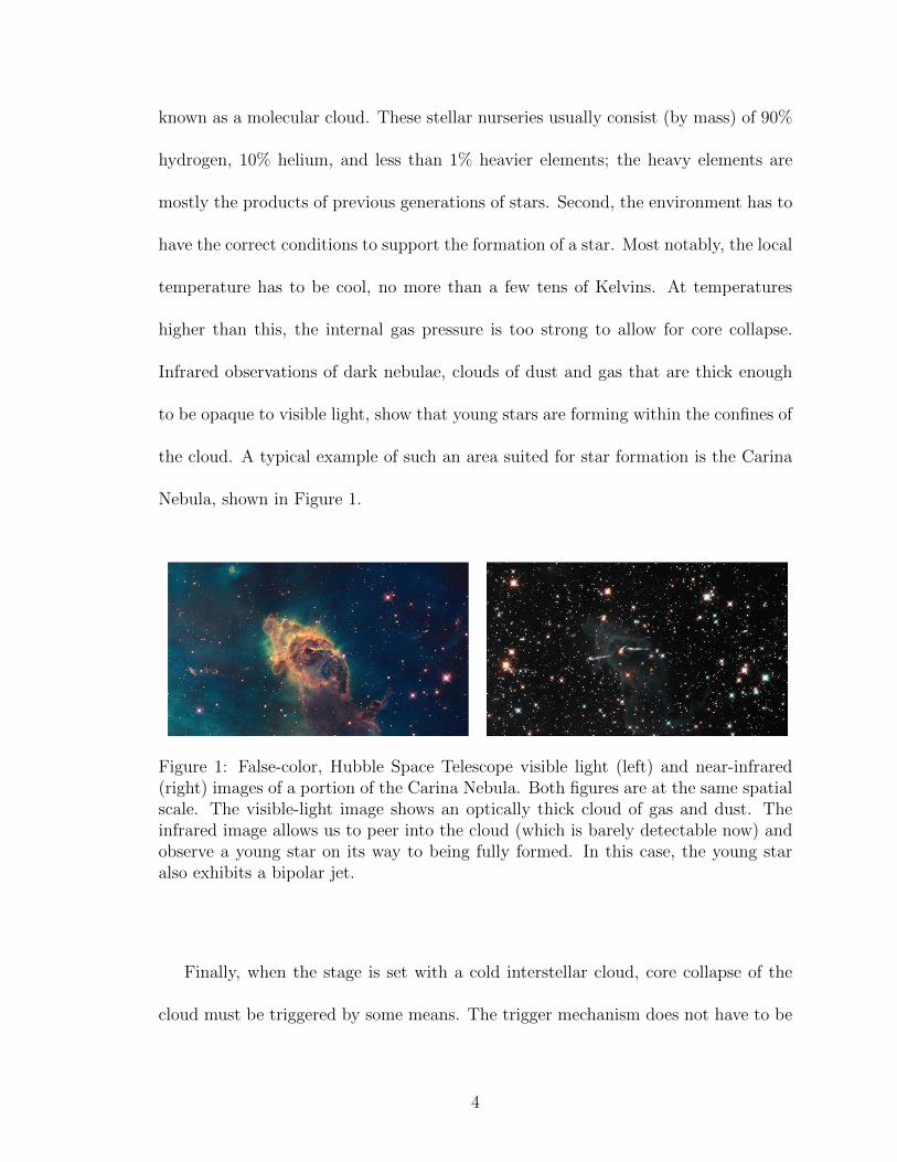
the cloud. A typical example of such an area suited for star formation is the Carina
Nebula, shown in Figure 1.
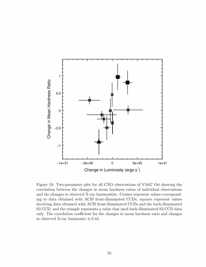
Figure 1: False-color, Hubble Space Telescope visible light (left) and near-infrared(right) images of a portion of the Carina Nebula. Both figures are at the same spatialscale. The visible-light image shows an optically thick cloud of gas and dust. Theinfrared image allows us to peer into the cloud (which is barely detectable now) andobserve a young star on its way to being fully formed. In this case, the young staralso exhibits a bipolar jet.
Finally, when the stage is set with a cold interstellar cloud, core collapse of the
cloud must be triggered by some means. The trigger mechanism does not have to be
4
violent. For example, radiation pressure of nearby stars can compress gas to create
an over-density of material in part of the cloud, which can start the collapse of part or
all of the cloud. Supernovae send out shockwaves that ripple through the interstellar
medium. When a pressure wave comes in contact with an interstellar cloud, a shock
forms as the high-speed wave slams into the slower-moving cloud, creating a region
of high over-density. Gravitational encounters between galaxies can lead to large
amounts of gas being stripped from each galaxy as they perform their gravitational
tango, leading to tidal tails millions of light-years long. As the gas clouds of one
galaxy are stretched and compressed by the gravitational influence of the interacting
galaxies, over-densities arise in the gas. This often gives rise to massive amounts of
star formation all at once, prompting astronomers to know many of these interacting
bodies as “starburst galaxies.”
In order to start the process of core collapse, even with all of the listed ingredients
and trigger mechanisms, the Jean’s stability must be overcome (Eq. 1.1).
dP
dr=
G⇢Menc
r2(1.1)
Equation 1.1 shows that the outward pressure P in a volume over a given distance
r is determined by the gravitational force that is trying to collapse the mass enclosed
inside the given volume (Menc) with a certain density ⇢. In an “inert” cloud, the
thermal pressure (and other internal forces such as support from a magnetic field) of
the material is in balance with the gravitational force. In order to start the collapse
of the cloud, the external trigger mechanism must apply enough force so that the
5
internal pressure will be overcome. Once this occurs, the resulting over-density in the
cloud has a stronger gravitational field, and a run-away process of contraction can
start.
As an interstellar cloud collapses in on itself, the original cloud begins to fragment
into separate clumps that each form a star. This is the main reason why, when sam-
pling a stellar population, one finds that most stars are not single. Much work has
been done to try and determine what factors lead to single or multiple-star forma-
tion. For example, Boss (2009) found through his three-dimensional hydrodynamic
modeling that the strength of the magnetic field that pervades the cloud, as well as
whether the initial rotating molecular cloud was prolate or oblate, has a significant
impact on whether single or multiple protostellar cores are formed during collapse.
However, the fragmentation process remains poorly understood.
1.1.1 Circumstellar Disks
In 1755, the German philosopher Immanuel Kant hypothesized that many of the
“fuzzy” celestial objects observed via telescopes were dusty clouds in the process of
forming stars and planets. In 1796, the French mathematician and astronomer Pierre-
Simon Laplace proposed a similar model, arguing that the nearly-circular orbits of
the planets were a direct result of the formation process (Woolfson, 1993). Today,
the general model put forth by Kant and Laplace is accepted as the formation the-
ory for the solar system. Usually known by names such as the Solar Nebula Disk
Theory, this model starts with a protostellar clump that is on its way to becoming a
fully-fledged star. Once a protostellar clump has formed within an interstellar cloud
6
and is contracting, its rotation speed as it collapses increases due to conservation of
angular momentum. The roughly spherical cloud begins to flatten as the centrifugal
force on the particles begins to counteract the gravitational force component that
is perpendicular to the spin axis; however, the remaining gravitational force compo-
nent, parallel to the spin axis, is not a↵ected. The particles begin to settle towards
a central plane perpendicular to the spin axis of the system. Over time, the once
roughly-spherical cloud becomes a central mass surrounded by a disk. Numerical
modeling of protostellar clumps indicates that this collapse phase lasts on the order
of ⇠106 years (Yorke & Bodenheimer, 1999).
The Laplace model of solar system formation, while successful at explaining the
overall structure of a solar system, was unable to fully explain how the Sun, with
over 99% of the mass of the solar system, accounts for less than 1% of the total
solar system angular momentum. Attempts had been made in the following years
at modifying this model, but each attempt usually gave rise to other unexplainable
issues. Prentice (1978) modified this formation model in such a way that the “Modern
Laplace Model” was able to correctly predict many of the observed properties of the
solar system including the angular momentum distribution. This model takes into
account the formation of dust grains in the center of the cold disk which impart drag
onto the collapsing disk. The gas at the center of the disk loses momentum and
further collapses to form a slowly-rotating sun which, in the end, has one-hundredth
of the total angular momentum of the disk. As the protostar’s temperature increases,
the dust grains evaporate while the planets continue to form in the faster-rotating
disk.
7
With advancements in telescope and detector technology, the Solar Nebula Disk
Theory has gained significant support, especially through direct observations of disks
around some objects. Figure 2 shows several prime examples of young stars with
disks seen both edge-on and face-on to our line of sight. Due to the substantial
amount of material orbiting the central stars, these circumstellar disks appear mostly
in silhouette with some reflected starlight illuminating the tops and bottoms of the
disks. In some of the image panes, bipolar jets associated with accretion are observed.
Figure 2: Edge-on circumstellar disks (left pane) and nearly face-on circumstellardisks (right pane) are observed mostly in silhouette around eight young stars. Im-age Credits: Chris Burrows (STScI), John Krist (STScI), Karl Stapelfeldt (JPL)and colleagues, the WFPC2 Science Team and NASA (left pane); Mark McCaugh-rean (Max-Planck-Institute for Astronomy), C. Robert O’Dell (Rice University), andNASA (right pane).
In many cases, especially when a target is very distant, direct observations of the
disks are not possible. However, the signatures of circumstellar disks can be found
8
in the spectra of star-disk systems. Modeling of stellar spectra allows astronomers
to determine many properties of stars. To nail down stellar parameters to within a
high confidence level, the observed spectrum of the star has to match a synthesized
spectrum very well. In the case of an “ordinary” star, the observed spectrum is usually
modeled fairly easily, especially if the star is not extremely faint and if there are no
peculiarities associated with the star’s spectrum. The observed spectrum of a star
surrounded by a circumstellar disk can be dramatically di↵erent, however, especially
when one observes the system at infrared and longer wavelengths. Figure 3 shows
the spectral energy distribution (SED) of the star GM Auriga, a star that is known
to have a circumstellar disk. The SED of a system such as GM Auriga exhibits a
flux contribution from the disk as well as from the star. The shorter wavelength
flux of the SED, primarily those of the optical, are contributed mostly by the star
itself. Longer wavelength data provide evidence of the disk. Instead of observing
the expected decline in flux past the optical wavelength regime, the flux actually
decreases much less due to the circumstellar material, which is radiating at infrared
wavelengths after being warmed by its star or by accretionary growth of the disk
itself. This “infrared excess” is the contribution of the disk to the SED. The bluer
wavelengths, which are contributed by the star, provide the spectral information that
allow one to model the stellar spectrum. This is not always an easy task as the more
heavily-embedded the object is, the redder it appears due to scattering of the bluer
wavelengths by intervening dust. If enough visible light emerges from the star-disk
system, then a stellar spectrum can be derived. With that, then by carefully studying
and modeling the shape of the infrared excess, one can determine many aspects of
9
the circumstellar disk, such as the inner disk radius, the vertical geometry of the disk,
and the inclination of the disk to our line of sight.
2003MNRAS.342...79R
Figure 3: Spectral energy distribution (squares) of GM Auriga overlaid with themodeled SED of the stellar photosphere (dotted line) and the combined modeledstellar and circumstellar disk SEDs (solid line) with the disk viewed at an inclinationof 50�. The disk begins 0.05 AU from the star and extends outwards to about 300AU. The dashed line represents the same SED but with the disk extending inward towithin 7 stellar radii instead of a having a large gap between the star and the innerdisk boundary. Figure adapted from Figure 3 of Rice et al. (2003).
When considering the life of a star, the presence of a circumstellar disk can be
considered a transient phase of a star’s evolution. By observing a multitude of stars
of various ages, each star gives us a snapshot into the stellar life cycle and allows
us to determine the expected circumstellar disk lifetimes. Haisch et al. (2001) used
measurements of infrared fluxes to determine the infrared colors of stars in six young
10
clusters. They found a strong correlation between the age of the cluster and the
fraction of stars in each of the clusters that show infrared excesses characteristic of the
presence of circumstellar disks. Starting with the youngest observed cluster (�80%
of cluster members possessed circumstellar disks), Haisch et al. (2001) found that the
cluster disk fraction decreased to 50% with an increase in age of approximately 3
Myr, suggesting that the overall disk lifetime of young stars is roughly 6 Myr.
Wolk & Walter (1996) observed 39 stars with strong infrared excesses and found
that some appeared to have “transition disks,” circumstellar disks that are in the
process of dispersal and that are transitioning from optically thick to optically thin.
By multiplying the fraction of stars observed to have transition disks with the mean
age of the stars, they deduced that circumstellar disks have an optically-thick lifetime
(the time it takes for the disk to go from optically thick to optically thin) of ⇠105 years.
After that, the disks are dominated by micron-size dust grains. The presence of disks
around stars older than a few million years is thought to be due to collisions of larger
bodies within the disks. If these debris disks were primordial, then the detected dust
out to ⇠10 AU should have been depleted in ⇠105 years due to Poynting-Robertson
drag (Mamajeck et al., 2004). The lifetimes of optically thick and optically thin disks
help to constrain planet formation theories in that we now know the typical periods
of time during which there are reservoirs of material out of which planets can form.
1.1.2 Circumstellar Accretion
On occasion, material will be perturbed in the circumstellar disk and accrete
onto the parent star through various mechanisms possibly involving gravitiational
11
perturbations or disk instabilities (e.g., see works by Clarke et al. (1989); Bell et al.
from the inner portion of the circumstellar disk. Such accretion is likely controlled
by magnetic flux tubes that connect the star to the disk.
YSOs are known to be quite magnetically active, as is often indicated by pro-
nounced CaII emission as well as observations of periodic transits of starspots (direct
manifestations of magnetic activity), which are derived from the observed modula-
tion of light curves (Stassun et al., 2006). Donati et al. (2007) have shown through
three-dimensional modeling that the stellar magnetic fields are intimately linked with
the magnetic fields of the circumstellar disk. During accretion, circumstellar material
is funneled along magnetic field lines and deposited at high stellar latitudes, where it
is shock-heated as it impacts the photosphere. The accretion footprint emits at ul-
traviolet and X-ray wavelengths. The accreting material above the footprint absorbs
and thermalizes radiation given o↵ at the shock, causing it to re-radiate this energy
at longer wavelengths. Since the material density is high near the accretion footprint,
this plasma often radiates more as a blackbody than as an optically thin gas. The
ultraviolet and optical emission thus comes in the form of a continuum overlaid on
top of the stellar spectrum. This accounts for the ultraviolet excess observed in the
spectra of many known accreting stars. In addition, the spectral features of accreting
stars are often “veiled;” that is, the absorption features, here mostly in the optical
wavelength regime, are e↵ectively filled in due to the presence of continuum emission.
Hydrogen-balmer emission lines are observed in the spectra of T Tauri stars and
are thought to result from absorption and re-emission of flux in the stellar atmosphere
12
produced by the accretion footprint. The hydrogen gas is excited and/or ionized, and
recombination of the ionized hydrogen and spontaneous emission from excited atoms
produces the characteristic observed hydrogen emission lines.
13
CHAPTER II
ERUPTING YOUNG STARS
2.1 T Tauri Stars
There are literally dozens of variable star classes. The majority of these, however,
involve fully formed main-sequence stars or, as in the case of many single star systems,
stars that have evolved o↵ the main sequence. Some of these variable star classes
consist of binary systems in which the components are physically interacting with
one another, typically causing the total observed flux to vary sporadically or quasi-
periodically. Other binary systems have components that are distant enough from
one another that they only interact gravitationally with one another. In these cases,
the stars’ orbital geometry causes them to eclipse one another, periodically varying
the observed flux. Still other variable star classes involve single, evolved stars that
pulsate. There are fewer variable star classes that exist which consist of very young
objects that have not reached the main sequence. This is often because these objects
are still deeply embedded in dusty regions, making many of them very di�cult to
observe or even notice in the first place.
When discussing the final formation of low-mass (2M� and smaller) stars, these
objects are often grouped into a category of stars known as T Tauri stars (TTSs),
named after the prototype T Taurus. T Taurus, or “T Tau”, was first noted in
1852 by John Russel Hind (Barnard, 1895). Joy (1945) suggested that this star,
along with ten others, should comprise a separate class of variable stars based on
14
spectroscopic and photometric characteristics. TTSs were found to vary irregularly
by several magnitudes, showed strong emission features in their spectra, had spectral
types that were indicative of lower mass stars, and were associated with nebulosity.
T Tauri stars are further categorized into “classical” T Tauri stars (cTTSs) and
“weak-line” T Tauri stars (wTTSs) based on the strengths of emission lines in their
spectra. WTTSs are considered by some to be in a later stage of TTS evolution and
may have shed most or virtually all of their disks. Walter (1986) suggested that these
stars are not post-T Tauri stars but should instead be considered “naked TTSs. One
of the major problems in the field of studying T Tauri stars is how to classify these
objects based on their spectral characteristics. In earlier work, a rule-of-thumb for
separating these stellar classes concerned the equivalent width of the hydrogen-alpha
emission line: if the equivalent width of the hydrogen-alpha emission line at 6563A
was greater than 10A for a TTS, then the star was considered a cTTS. If the hydrogen-
alpha equivalent width was less than 10A or in absorption), then the star was classified
as a (wTTS). As many have found, this classification scheme is not extremely robust.
For instance, it can be di�cult to determine, based on the hydrogen-alpha line pro-
file, whether or not the star is accreting even though the hydrogen-alpha spectral
line is in emission. Kurosawa et al. (2006) used several di↵erent models to simulate
classical T Tauri stars that were exhibiting hydrogen-alpha emission. They found,
for example, that some scenarios could produce the required hydrogen-alpha equiva-
lent width through magnetospheric accretion, but other models that were dominated
by disk-wind emission produced similar equivalent widths. A more robust classifica-
tion method that makes use of the hydrogen-alpha cuto↵ was suggested by Martın
15
(1997). Once the TTS spectral classification has been determined, the equivalent
width corresponding to the maximum amount of hydrogen-alpha emission that can
be produced by the star solely from an active chromosphere (excluding things such
as flares) is modeled. The amount of hydrogen-alpha emission above the calculated
maximum value is therefore likely a product of accretion. For instance, equivalent
widths greater than ⇠10A for early-M and ⇠20A for late-M spectral types would be
indicative that accretion is occurring.
WTTSs do not possess strong emission features like their cTTS counterparts,
so they have fewer spectral characteristics that set them apart from regular main
sequence stars. In the case where circumstellar accretion has decreased such that
emission lines are no longer present in the stellar spectrum, a wTTS would be di�cult
to distinguish from a main sequence star. Since these stars are very young, the 7Li
absorption feature at 6708A1 has been found by some to be a good indicator that
a star might be a wTTS. Martın (1997) assumed that all TTSs will have an initial
lithium abundance and that the abundance should not be significantly a↵ected for
stars younger than 10 Myr. He then calculated the minimum lithium equivalent
width that these stars should have, which is mostly dependent on the stellar e↵ective
temperature, and found that the predicted equivalent widths are indeed higher than
what is observed for young clusters, such as the Pleiades (age ⇡ 100 Myr).
Due to the young ages of these stars, most TTSs still possess circumstellar disks,
1As stars age, convection e↵ectively mixes their outer layers, and the lithium is transported intothe lower convective layers where it is photo-dissociated by the higher temperatures. Thus, as starsage and the lithium in the outer part of the star is depleted, the equivalent width of the lithiumspectral features decreases.
16
which provide mass reservoirs from which the stars can grow through circumstellar
accretion. Typical mass accretion rates for T Tauri stars are around 10�9–10�8 M�
yr�1 (Calvet et al., 2004), though this value can vary widely. Accretion of circumstel-
lar material onto the central star results in flux increases in the X-ray through infrared
wavelength regimes and also causes the star to appear variable as the accretion rate
fluctuates or the accretion stream geometry changes. In addition, infalling material
absorbs some of the bluer flux from the emission line, reducing the overall amount of
the blue-wing emission of some emission features. In cases where the absorption is
strong enough, the emission line blue wings go into absorption while the remainder
of the feature stays in emission, producing what is known as an inverse P-Cygni pro-
file.As material impacts the photosphere, the energy generated also ejects material
from the star, generating a wind. The signature of this wind is observed in cTTS as
a P-Cygni profile in the prominent emission lines. Though a wind would be expected
to be produced in any direction (such that a redshifted and blueshifted component
should be observed), the blueshifted wind component is observed most due to the
optically thick circumstellar disk blocking our view of the redshifted component.
2.2 FUors and EXors
There are two prominent classes of cTTSs that are known to erupt because of
sudden, large-scale accretion events: FUors and EXors. In general, it is thought
that the main di↵erence between these types of stars is the level of their “quiescent”
accretion rates and the duration and magnitude of the large accretion episodes that
they experience. Figure 4 illustrates they physical setup of these types stars and how
17
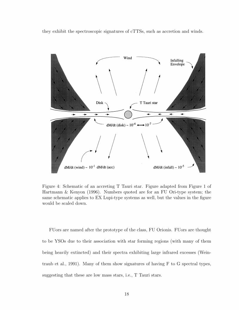
they exhibit the spectroscopic signatures of cTTSs, such as accretion and winds.
July 24, 1996 14:50 Annual Reviews HARTTEX1 AR12-06
208 HARTMANN & KENYON
accreted in FU Ori outbursts reinforce the notion that disk accretion plays amajor role in the formation of stars and not just their associated planetary sys-tems. FUOri outbursts also demonstrate that accretion rates through such diskscan be highly time variable and unexpectedly large at times, with implicationsfor disk physics and grain processing. Finally, the powerful winds of FU Oriobjects have important implications for understanding the production of bipolaroutflows and jets.Figure 1 summarizes the current picture of a typical FU Ori object. A young,
low-mass (TTauri) star is surroundedby a disk normally accreting at⇠ 10�7 M�
yr�1. This slow accretion is punctuated by occasional, brief FUOri outbursts, inwhich the inner disk erupts, resulting in an accretion rate⇠ 10�4 M
�yr�1. The
disk becomes hot enough to radiate most of its energy at optical wavelengths,and it dumps as much as 0.01 M
�onto the central star during the century-long
Figure 1 Schematic picture of FU Ori objects. FU Ori outbursts are caused by disk accretionincreasing from ⇠ 10�7 M� yr�1 to ⇠ 10�4 M� yr�1, adding ⇠ 10�2 M� to the central T Tauristar during the event. Mass is fed into the disk by the remanant collapsing protostellar envelopewith an infall rate <
⇠10�5 M� yr�1; the disk ejects roughly 10% of the accreted material in a
high-velocity wind.
Ann
u. R
ev. A
stro
. Ast
roph
ys. 1
996.
34:2
07-2
40. D
ownl
oade
d fr
om w
ww
.ann
ualre
view
s.org
by V
ande
rbilt
Uni
vers
ity o
n 01
/18/
11. F
or p
erso
nal u
se o
nly.
Figure 4: Schematic of an accreting T Tauri star. Figure adapted from Figure 1 ofHartmann & Kenyon (1996). Numbers quoted are for an FU Ori-type system; thesame schematic applies to EX Lupi-type systems as well, but the values in the figurewould be scaled down.
FUors are named after the prototype of the class, FU Orionis. FUors are thought
to be YSOs due to their association with star forming regions (with many of them
being heavily extincted) and their spectra exhibiting large infrared excesses (Wein-
traub et al., 1991). Many of them show signatures of having F to G spectral types,
suggesting that these are low mass stars, i.e., T Tauri stars.
18
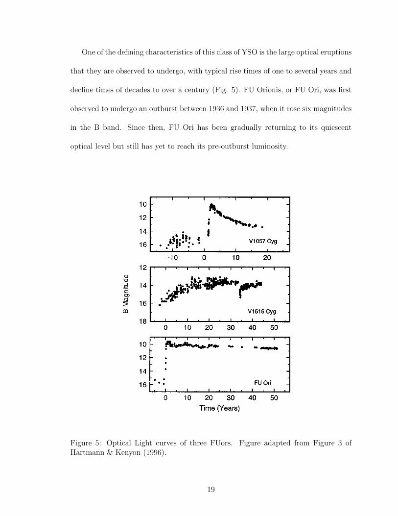
One of the defining characteristics of this class of YSO is the large optical eruptions
that they are observed to undergo, with typical rise times of one to several years and
decline times of decades to over a century (Fig. 5). FU Orionis, or FU Ori, was first
observed to undergo an outburst between 1936 and 1937, when it rose six magnitudes
in the B band. Since then, FU Ori has been gradually returning to its quiescent
optical level but still has yet to reach its pre-outburst luminosity.
July 24, 1996 14:50 Annual Reviews HARTTEX1 AR12-06
FU ORIONIS PHENOMENON 211
kilometers per second, is typically observed in the Balmer lines, especially inH↵. The Na I resonance lines also show broad blueshifted absorption, some-times in distinct velocity components or “shells.” The emission component inthe P Cygni H↵ profile is often absent; when present, this emission extendsto much smaller velocities redward than the blueshifted absorption. Infraredspectra of FUOris show strong CO absorption at 2.2µm and water vapor bandsin the near-infrared (⇠ 1–2 µm) region. The near-infrared spectral character-istics are inconsistent with the optical spectra, if interpreted in terms of stellarphotospheric emission; the infrared features are best matched with K–M giant-supergiant atmospheres (effective temperatures of ⇠ 2000–3000 K). FGKMsupergiants are rare in any case and are not commonly found in star formationregions; thus, optical and near-infrared spectra serve to identify FUOri systemsuniquely.
Figure 3 Optical (B) photometry of outbursts in three FU Ori objects. The FU Ori photometryis taken from Herbig (1977), Kolotilov & Petrov (1985), and Kenyon et al (1988); the V1057Cyg photometric references are contained in Kenyon & Hartmann (1991); and the V1515 Cygphotometry is taken fromLandolt (1975, 1977), Herbig (1977), Gottlieb&Liller (1978), Tsvetkova(1982), Kolotilov & Petrov (1983), and Kenyon et al (1991b).
Ann
u. R
ev. A
stro
. Ast
roph
ys. 1
996.
34:2
07-2
40. D
ownl
oade
d fr
om w
ww
.ann
ualre
view
s.org
by V
ande
rbilt
Uni
vers
ity o
n 01
/18/
11. F
or p
erso
nal u
se o
nly.
Figure 5: Optical Light curves of three FUors. Figure adapted from Figure 3 ofHartmann & Kenyon (1996).
19
FUors have typical accretion rates of 10�7 M� yr�1, but the accretion rate rises
by up to three orders of magnitude during large optical outbursts. During these
large outbursts, the disk radiates most at optical wavelengths and can easily outshine
its companion star (Hartmann & Kenyon, 1996). The eruptions are not thought
to be due to dramatic changes in intervening extinction since the spectral features
change when observing the star going from its minimum to its maximum optical level
or visa versa (Herbig, 1977). However, with strong evidence to suggest that FUors
are surrounded by circumstellar disks, it is thought that the observed eruptions are
due to massive accretion events from the circumstellar disk. FUors were some of
the first objects to have their outbursts explained successfully with a disk-accretion
model (Lin & Papaloizou, 1985). Spectroscopic observations show absorption feature
doublets (i.e., red-shifted and blue-shifted absorption lines), which are not character-
istic of line broadening due to a fast-rotating star but are instead characteristic of
material orbiting the star (Fig. 6). As one examines absorption features at longer
wavelengths, the spread of the double-features decreases. Material (which is radiating
as a blackbody in an optically-thick disk) would be cooler, orbiting at a slower rate,
and radiating in longer wavelengths the farther out in the disk it is located. Thus,
the longer-wavelength spectral doublets are indicative of material orbiting farther out
from the star.
Hartmann & Kenyon (1996) determined that if one low-mass star were formed ev-
ery 100 years for a 1kpc cylinder centered on the Sun, then given that there have been
approximately five FUor outbursts in 60 years (as of 1996), then FU Ori outbursts
should occur approximately 10 times for each low-mass star. Therefore, if the out-
20
July 24, 1996 14:50 Annual Reviews HARTTEX1 AR12-06
FU ORIONIS PHENOMENON 221
to accomplish this spectrum synthesis by using standard supergiant stars. Thecomparison between the spectra of disk models constructed in this way and theFU Ori spectra is remarkably good (Kenyon et al 1988).Not all absorption lines in FU Ori are doubled, particularly those in the
blue spectral region (Petrov & Herbig 1992). As discussed in Section 5, theobservations suggest that the line doubling is masked by the expansion of thedisk surface in an accelerating wind (Hartmann & Kenyon 1985, 1987a; Calvetet al 1993).
3.1.4 ROTATION VSWAVELENGTH The disk model predicts that the rotationalvelocity line broadening observed at infrared wavelengths should be very largein comparison with typical evolved stars, which are slowly rotating, but smallerthan the optical line broadening, because the optical lines are produced in morerapidly rotating inner disk regions. In Figure 7, the uppermost spectrum isthat of the M giant HR 867, which exhibits strong, sharp CO vibration-rotationabsorption lines. Even though the spectra of the FU Ori objects V1057 Cygand FU Ori are noisier, their larger velocity broadening is apparent, especiallyfrom the shape of the bandhead. The dotted line is a model disk spectrum, inwhich the rotational broadening is calculated by scaling the disk model rotation
Figure 6 High-resolution optical spectra of three FU Ori objects, showing line profile doublingat different velocity widths. The dotted curve illustrates the spectrum synthesized for a disk modelconstructed for comparison with FU Ori (see text).
Ann
u. R
ev. A
stro
. Ast
roph
ys. 1
996.
34:2
07-2
40. D
ownl
oade
d fr
om w
ww
.ann
ualre
view
s.org
by V
ande
rbilt
Uni
vers
ity o
n 01
/18/
11. F
or p
erso
nal u
se o
nly.
Figure 6: Portions of spectra of three FUors. The prominent absorption featuresshow line-doubling. The thinner line under the spectrum of FU Ori represents a diskspectrum model for FU Ori. Figure adapted from Figure 6 of Hartmann & Kenyon(1996).
burst lasts a century, as appears to be the case for FU Ori itself, then low-mass stars
could gain a significant amount of their final mass through these outburst episodes.
This amount could be much higher, especially given that FUors tend to be located
in heavily-reddened locations so that we may not be able to observe these eruptions
very often.
Calvet et al. (1991) was able to successfully model the spectral contribution of the
circumstellar disk for FUors. They assumed that the disk was in vertical hydrostatic
21
and radiative equilibrium and that the temperature varied as a function of radius
in the disk. Calvet et al. (1991) then split up the disk into many concentric annuli
and modeled each annulus in a stellar atmosphere radiative transfer method. From
each model, an e↵ective temperature and surface gravity were derived. They then
combined the modeled spectral contributions from each annulus to determine the
total spectral contribution of the disk. The spectrum of FU Ori was also modeled
in this manner, and they were able to use the disk contribution to account for the
optical spectral energy distribution of FU Ori itself, strongly suggesting that the disk
of FU Ori outshines FU Ori. In addition, they found that the contribution of FU
Ori to the heating of the disk is negligible (it was neglected in the modeling and not
needed to get the modeled spectrum to fit the data) and that the presence of the
strong absorption features indicates that the disk is also very optically thick.
EXors comprise another class of erupting star that is named after the prototypical
star, EX Lupi. EXors are similar in some aspects to FUors, but they also have
their di↵erences that set them apart from FUors. EXors, however, have much lower
maximum accretion rates as compared to FUors, and the rise times and subsequent
decline times of optical outbursts are on the order of weeks and months to a few
years, respectively. EXors are also observed to undergo optical outbursts much more
frequently than FUors. EX Lupi, for example, was first observed to erupt in in 1901,
with six later eruptions through 2008. Thus, EX Lupi has erupted nearly as many
times during the typical span of one FUor outburst as what is predicted for a typical
FUor.
During the 2008 “extreme” outburst of EX Lupi, the veiling-corrected accretion
22
rate was found to be 2 ⇥ 10�7 M� yr�1, which is approximately 40 times greater than
the accretion rate during optical quiescence (Aspin et al., 2010). As compared with
the quiescent accretion rate 10�7 M� yr�1 for FU Ori, the accretion rates of EXors
are found to be on the order of the quiescent accretion rates of FUors even when
undergoing major outbursts.
23
CHAPTER III
X-RAY ASTRONOMY: A TOOL FOR STUDYING YOUNG STARS
3.1 Previous X-ray Work
The most obvious feature of the night sky is the thousands of stars that one
can observe with the naked eye. Once the science of astronomy had evolved to the
point of trying to use scientific means to derive information about the world and
the universe itself, we naturally asked questions about these shimmering nighttime
visitors. We began by observing what we could with our eyes, noting things such as
brightness, color, and whether the stars appeared to vary in any way over time. With
the invention of the optical telescope in 1609, we were able to increase our observing
capabilities, as well as our understanding of stars, by many orders of magnitude.
With the discovery of other types of light, such as infrared and ultraviolet, we began
to ponder if these other forms of light might be tools to investigate other aspects of
stars. We discovered in the twentieth century that our understanding of the lives of
stars, and not just physical measurements of stars, would be greatly expanded with
the use of infrared light, which allowed us to see into the dark, invisible portions of the
celestial sphere and peer into dark molecular clouds and witness some of the earliest
moments of a star’s birth and development. A tremendous amount of work done
in observing young stars in the optical and infrared wavelength regimes; however,
the volume of literature regarding X-ray studies of young stars, especially cTTSs
and wTTSs, is smaller. With optical and infrared light revealing so many secrets
24
of the lives of stars, what information could X-ray astronomy provide us, especially
with regards to the lives of young stars? One of the big questions that is still not
well answered is why many young stars, especially lower mass stars, are such strong
sources of X-rays. X-ray studies of such objects are important for improving our
understanding of the evolution of a star as well as of its circumstellar environment,
in which planetary systems may be forming. Thus, X-ray observations of stars give
us a glimpse into how the X-ray behavior of T Tauri stars like our nascent Sun a↵ect
the evolution of stellar systems.
The first observations of X-ray emission from T Tauri stars were made by the
Einstein X-ray Observatory. Feigelson & DeCampli (1981) found eight sources in the
Taurus and Orion star-forming regions that had X-ray luminosities of ⇠1030–1031 ergs
s�1, roughly three to four orders of magnitude greater than the Sun’s X-ray luminosity
of ⇠1027 ergs s�1 (Orlando et al., 2001). They concluded that due to the rapid X-
ray variability of some of these stars (e.g., a ⇠4-minute significant increase in X-ray
luminosity in DG Tau), the high X-ray luminosity was likely produced near the stellar
photosphere. Since then, astronomers who study X-rays from TTSs have identified
di↵erent X-ray generation mechanisms, including solar-like coronal loops that are
larger than the radius of the star, accretion shocks, and magnetic reconnection in
accretion streams.
3.1.1 X-ray Production & Rotation
Previous work has found that there is sometimes a correlation between the rota-
tion period of a non-accreting star and its X-ray luminosity. Specifically, the ratio
25
of the X-ray luminosity (LX) to the bolometric luminosity (Lbol) increases with de-
creasing rotation period. Vilhu & Rucinski (1983) found that there also appears to
be a “saturation level” of LX/Lbol ' 10�3 for G-K type stars with rotation periods
shorter than 2–3 days. Wright et al. (2011) found that this may be due to the way
that X-rays are generated via dynamo mechanisms inside the star (Fig. 7). Their
findings suggest that the dominant X-ray generating mechanism for fast rotators is a
convective (turbulent) dynamo and, as the stars age and their rotation periods have
increased to a certain point (⇠2–3 days), the dominant dynamo mechanism switches
to an interface-type dynamo. Therefore, once the rotation period of a “saturated”
star has decreased past ⇠2–3 days as the star ages, it appears that the dynamo mech-
anism changes and the value of LX/Lbol decreases such that the star then falls into
the “unsaturated” X-ray regime.
For the Sun, X-ray activity is the result of magnetic activity heating the coronal
plasma to X-ray-emitting temperatures. The complex magnetic field of the Sun is
thought to be a combination of e↵ects, primarily from an “↵!-dynamo.” In this
picture, the di↵erential rotation of the Sun will cause the once-poloidal magnetic field
lines to be e↵ectively wrapped around the Sun (the “!” e↵ect), while these wrapped
magnetic field lines themselves twist due to rotation e↵ects on magnetic flux tubes
rising from deep within the Sun (the “↵ e↵ect”). The Sun, however, is di↵erent
from T Tauri stars in terms of internal structure. The Sun has a radiative zone
that extends from the core to roughly three-fourths of the solar radius, while the
remaining outer portion of the Sun transports the bulk of the generated energy via
convection. This structure allows for the creation of an “interface dynamo” at the
26
6
Fig. 2.— X-ray to bolometric luminosity ratio plotted against rotation period (left panel) and the Rossby number, Ro = Prot/� (rightpanel), for all stars in our sample with X-ray luminosities and photometric rotation periods. Stars known to be binaries are shown as plussymbols, and the Sun is indicated with a solar symbol. The best-fitting saturated and non-saturated activity–rotation relations describedin the text are shown as a dashed red line in the right-hand panel.
log C+� log Ro to all stars with Ro � 0.2 using the di↵er-ent types of linear regression fits in Isobe et al. (1990).We find a good agreement between the slopes derivedfrom these di↵erent fits, suggesting that the fits are allfairly linear in the log RX – log Ro plane. We favorthe Ordinary Least Squares (OLS) bisector since theobjective of the fit is to estimate the underlying func-tional relation between the variables, as recommendedby Isobe et al. (1990), and this method also factors in thescatter of the line in both variables. The fit gives a slopeof � = �2.55 ± 0.15 (valid in the range 0.2 < Ro < 3,or �3.75 > log(LX/Lbol) > �6.3), significantly steeperthan both the canonical value and that found from ourtwo-part fit. Mamajek & Hillenbrand (2008) fit a log-linear function to the RX � Ro distribution, with thegoal of empirically deriving a correlation that would al-low age estimates to be derived from X-ray luminosities(via rotation periods). Their fit does not connect withthe level of saturated X-ray emission for very fast rota-tors but, as they note, it o↵ers a good fit to many of theslow rotators such as the Sun.
The sample used here su↵ers from a number of biasesdue to the selection of only sources with measured X-ray fluxes and photometric rotation periods. While thebiases stemming from the detectability of rotation pe-riods are myriad and complex, the luminosity bias in-duced by only using sources with measured X-ray fluxesis clear. This bias will be most prominent in the unsat-urated regime where X-ray luminosity ratios may reachas low as ⇠ 10�7 or lower. This sample could there-fore be missing some of the faintest sources at a givenRossby number, possibly resulting in a larger spread inthe RX � Ro diagram than is currently observed. Sucha spread could easily be induced by the increased am-plitude of stellar coronal cycles that has been suggestedto occur as stars age (e.g. Micela & Marino 2003). Atthe largest Rossby numbers it is likely that many of thefaintest X-ray sources are not detected, inducing a strongbias in our sample that will a↵ect the fits derived here.
3.1.1. Probing the dynamo e�ciency with an X-rayunbiased sample
To overcome the biases in our large sample we haveattempted to compile from within our sample a smaller,X-ray unbiased sample that covers a large range in X-ray luminosity ratios and rotation periods. For this weuse the list of 36 Mt. Wilson stars with rotation periodsfrom the study by Donahue et al. (1996), all of whichwere detected by ROSAT and therefore do not su↵erfrom X-ray luminosity biases. These 36 stars are thesubsample of their entire sample of 100 observed starswith measurable rotation periods over five or more sea-sons. The authors discuss a number of possible biases intheir sample resulting from e↵ects such as active regiongrowth and decay, multiple active regions, and latitudi-nal bands. They conclude that the resulting biases a↵ectonly �P , not the period itself, and are either small or actto reduce the measured value of �P . Therefore we be-lieve that this sample of 36 stars with measured rotationperiods and and X-ray luminosities is free from the ma-jority of biases. These stars were included in our sampleas part of the compilations of Pizzolato et al. (2003) andMamajek & Hillenbrand (2008), and in Figure 3 we showtheir distribution in the RX–Ro diagram, all of which fallin the unsaturated regime of coronal emission.
We fitted a simple single-part power law of the formlog RX = log C + � log Ro to these points, using an OLSbisector (Isobe et al. 1990), though the slopes derivedfrom all the di↵erent fitting methods are in good agree-ment. The fit gives a slope of � = �2.70 ± 0.13 (valid inthe range 0.3 < Ro < 3, or �4 > log(LX/Lbol) > �6.3),steeper than that found from our larger sample, in agree-ment with our predictions of the uncertainties induced bythe biases of that sample. This slope is even steeper thanthe canonical value of � = �2 as well as the slope foundby Pallavicini et al. (1981) of � = �1.9 ± 0.5, thoughtheir use of projected rotational velocities instead of ro-tation periods represents a di↵erent relationship thanthat fitted here. However this slope is in good agree-ment with Gudel et al. (1997) who derive a similar slope,
Figure 7: Figure 2 adapted from Wright et al. (2011) displaying X-ray to bolometricluminosity ratio (RX) plotted against rotation period (Prot)(left panel) and the Rossbynumber (Ro)(right panel) for all stars in the Wright et al. (2011) sample with X-rayluminosities and photometric rotation periods. Stars known to be binaries are shownas plus symbols, and the Sun is indicated with a solar symbol. These data show that(RX) increases with decreasing (Prot) and decreasing (Ro) up to a limit, at whichpoint (RX) saturates. The best-fitting saturated and non-saturated activity-rotationrelations are shown as a dashed red line in the right-hand panel.
boundary between the radiative and convective zone which can generate a magnetic
field. T Tauri stars, on the other hand, are fully convective, and thus are unable to
create an ↵!-dynamo. As a result, theorists now believe that fully convective stars
are able to generate magnetic fields via a “turbulent” dynamo that is only weakly
dependent on the rotation of the star.
Flaccomio et al. (2005) reanalyzed the results of Chandra Orion UltraDeep Project
(COUP), a 2003 survey consisting of an 850 ks Chandra observation of the Orion
Nebula Cluster (ONC). Flaccomio et al. (2005) specifically searched for clues as to
how X-ray emission of ONC stars is related, if at all, to rotation. Restricting their
analysis to stars with known rotation periods as well as using both unfiltered and
27
filtered light curves (which had large flares removed), they found that only 10% of
their sample of stars showed evidence for X-ray modulation from rotation. In addition,
they determined that the “X-ray saturation” that was observed in some of the sample
is not due to the filling of the stellar photosphere with active regions and that the
dominant X-ray emitting structures are smaller than the stellar radii.
3.1.2 X-ray Production & Coronal Structures
Surveys of the emission measure2-temperature distribution of many active binary
stars (e.g., Sanz-Forcada et al. (2003)) found that there is often a prominent hot
plasma component, at roughly 10 MK, along with a cooler plasma component similar
to that found in the solar corona. Cargill & Klimchuk (2006) determined from their
modeling results that the 10 MK plasma component is likely due to the presence of
numerous small (loop height ⇠ few thousand km), dense (electron densities ⇠ 1012
cm�3) coronal loops that are similar to, but much denser than, those found in the
Sun.
Favata et al. (2005) found that a number of YSOs in the ONC produced large
flares during the COUP observations. Models of these flares showed that many of
them had loop heights that were on the order of at least 10 times the radius of the
host star. With such large loop heights, Favata et al. (2005) concluded that these
coronal loops, which confine the plasma responsible for the observed X-ray flares, also
connect the stellar photosphere and accretion disk, allowing them to channel material
falling from the circumstellar disk to the star during accretion.
2Emission measure is a determination of the amount of plasma contributing to observed emission.
28
3.1.3 X-ray Production & Accretion
One of the possible X-ray generation mechanisms is accretion of material from a
circumstellar disk. Calvet & Gullbring (1998) determined that material near free-fall
velocity can be shock-heated due to the large velocity gradient. They find that the
plasma temperature, according to strong-shock theory, is given by
TS ⇡ 3.5M
M�
✓R
R�
◆�1
[MK]. (3.1)
Substituting values for the radius and mass of typical TTSs (M = 0.1–1 M� and R
= 0.5–2 R�) into Equation 3.1, the expected shock temperature is TS ⇡ 0.4–4 MK,
which corresponds to an X-ray temperature of kTX ⇡ 0.035–0.35 keV.
Stassun et al. (2006) searched for a possible link between X-ray production and
accretion using COUP data and time-correlated BVRI photometry of young stars
in the ONC. With accretion known to produce increases in optical flux, variability
in optical flux (due to accretion) that is correlated with variability in X-ray flux
would suggest that both flux variations are the result of accretion. Stassun et al.
(2006) found that only 5% of their sample showed any correlation/anti-correlation
between X-ray and optical variations, suggesting that accretion hotspots in the stellar
photosphere are not dominant sites of X-ray production. However, it is still unclear
as to why there is sometimes a correlation between optical and X-ray flux in some
objects and not others when there are no observable characteristics that distinguish
the stars in the 95% group from those in the 5% group.
29
3.1.4 Gleaning Other Information from X-rays
X-ray line profiles have also been used to determine characteristics of stars. Helium-
like triplets (spectral features usually comprised of three spectral lines - a forbid-
den, an intercombination, and a resonance feature) can be used to determine plasma
characteristics such as electron temperature and density. For example, the K-shell
helium-like3 transitions consist of a resonance line, two intercombination lines, and a
forbidden line. The forbidden transition, which is observed to occur only at very low
densities, can be collisionally excited to the excitation level of the intercombination
lines. As density increases, the likelihood that an electron in the excited forbidden
state will be excited to an intercombination energy state increases as the likelihood
that an electron in the excited forbidden level will radiate spontaneously before be-
ing collisionally excited/de-excited decreases. Thus, the ratio of the forbidden to
intercombination line strengths provides a proxy for density.
Kastner et al. (2002) observed the wTTs TW Hydra in 2000 with the Chandra
X-ray Observatory using the High Energy Transmission Grating System and ACIS-S
(CXO instruments will be in §3.2) . TW Hydra is known to be accreting due to the
presence of hydrogen-balmer emission; however, determining the accretion rate from
this line profile alone is often di�cult to do with low uncertainty. The He-like Ne IX
was observed in the high-resolution X-ray spectrum, and the relative line strengths
were used to determine the electron density. After modeling the X-ray spectrum and
deriving other plasma parameters such as emission measure, Kastner et al. (2002)
were able to determine that the filling factor (the percentage of the stellar surface
3Helium-like refers to ions that have only have two bound electrons.
30
exhibiting this plasma) was much smaller than what is observed for normal coronal
X-ray sources. They concluded that the plasma generating these spectral features
likely arises from accretion hotspot(s) on the stellar photosphere. With the derived
electron density and using an assumed filling factor and accretion stream velocity, the
accretion rate was calculated for this object.
The X-ray spectrum of YSOs can also yield information about the circumstellar
environment. The most notable example is the fluorescence of “cold” iron (iron that
is weakly ionized) in the cirumstellar disk. Iron emission lines are often observed
in the X-ray spectra of YSOs in the 6.7–7.0 keV range. This feature is the He-like
Fe K↵-line triplet at 6.64, 6.67, and 6.70 keV. More recently, a neutral iron K-↵
doublet at 6.4 keV has been observed in the spectra of some YSOs, including those
that are heavily embedded. These emission lines are the result of higher-energy X-ray
photons (energy�7.11 keV) weakly ionizing iron atoms or ions through the removal
of a 1s electron. Imanishi et al. (2001) provided the first detection of the neutral iron
doublet in the X-ray spectrum of a deeply embedded YSO when observing YLW 16A
in ⇢ Ophichus (Fig. 8), and this feature was also detected in the X-ray spectrum of
objects, such as V1647 Ori (Grosso et al., 2005; Teets et al., 2011) and seven sources
in the ONC (Tsujimoto et al., 2005).
31
~6.4 keV
~6.7 keV
758 IMANISHI, KOYAMA, & TSUBOI Vol. 557
Fig. 9a
Fig. 9b
FIG. 9.È(a) Light curve of YLW 16A (No. 57 ; upper) and time pro!le ofthe best-!t temperature (middle) and the emission measure (lower). (b) Spec-trum of YLW 16A in phases 7È9. The upper panel shows data points(crosses) and the best-!t model (solid line), while the lower panel showsresiduals from the best-!t model. Line structures are seen at 6.4 and 6.7keV.
brightest Ñare seen in YLW 16A (see ° 4.8.5) but may not beextraordinary. Subsequent ASCA observation discoveredthree quasi-periodic X-ray Ñares with an interval of D20 hr(Tsuboi et al. 2000). These Ñares are interpreted with a star-disk arcade conjecture (Montmerle et al. 2000), with anX-ray emission mechanism somehow di†erent from that of
Fig. 10a
Fig. 10b
FIG. 10.È(a) Light curve of ROX 21 (No. 40) for the total X-ray band.The solid line represents the best-!t (exponential]constant) model. (b)Spectra of ROX 21 (No. 40) in the Ñare (black) and quiescent (gray) phases.
class II]IIIs, which may have magnetic arcades within thestar. Although Chandra con!rms the hard X-ray emissionand !nds a typical Ñare from YLW 15A (Fig. 2h), no multi-ple Ñares are found. Thus, quasi-periodic Ñares are notalways present but rather occasional phenomena.
4.8.5. Y L W 16A (No. 57)
The light curve of YLW 16A seems to be comprised oftwo Ñares : the !rst is rather complex with several spikelikestructures, and the second is a giant Ñare of unusual pro!le(Fig. 9a). We examine the spectral evolution by slicing thedata in time as shown in Figure 9a. In phases 7È9, weextract the spectra from the same region (a radius2A.5È7A.5annulus) as the light curve data because these phases su†erfrom the pileup e†ect (see ° 3.3). We !rst !t the spectra witha thin thermal model allowing the abundance and to beNHfree for all the phases, and we !nd no signi!cant variationfrom phase to phase in both abundance (0.3 solar) and NH.We hence !x the abundance to be 0.3 solar and !t thespectra assuming that is consistent in all the phases. TheNHbest-!t parameters for each time interval are shown inTable 3. As seen in Figure 9a, the temperature (kT ) and EM
Figure 8: X-ray spectrum of YLW 16A (crosses) and the best-fit model (solid line),while the lower panel shows residuals from the best-fit model. The 6.4 and 6.7 keVspectral features are accounted for with the addition of two Gaussians (shown by thedot-dashed and dotted lines, respectively. Figure adapted from Figure 9b of Imanishiet al. (2001).
32
3.2 The Chandra X-ray Observatory
Launched from the Space Shuttle Columbia on July 23, 1999, the 45-foot long
Chandra X-ray Observatory (CXO) is an orbiting X-ray telescope and the third of
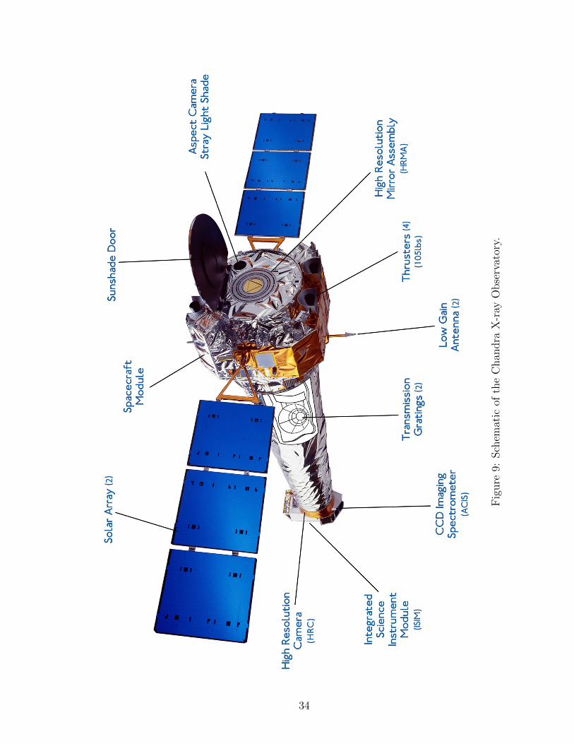
NASA’s four “Great Observatories.” CXO (Fig. 9) is named after Subrahmanyan
Chandrasekhar, the Nobel prize-winning physicist most noted for first calculating the
mass limit of a white dwarf. Chandra’s rather eccentric orbit takes it into a high Earth
orbit, putting it above the Van Allen belts for most of its 64.3-hour orbital period and
allowing for roughly 55 hours of continuous observation time. The Chandra X-ray
Observatory is unique in that it has the highest spectral and spatial resolutions thus
far of any orbiting X-ray observatory – up to 0.012A (or 1 eV) at Full Width Half
Maximum (FWHM) and up to to 0.500 at FWHM, respectively. Chandra’s spectral
range is 0.3–10 keV, and though other X-ray observatories such as XMM-Newton
provide a wider calibrated spectral energy range, they have a lower spectral resolution.
The Chandra X-ray Observatory has a suite of instruments and components, including
the High Resolution Mirror Assembly (HRMA), the High Resolution Camera (HRC),
the Advanced CCD Imaging Spectrometer (ACIS), and the Low- and High-Energy
Transmission Gratings (LETG/HETG), which allow it to make a number of various
types of X-ray observations.
33
Figure
9:Schem
atic
oftheChan
dra
X-ray
Observatory.
34
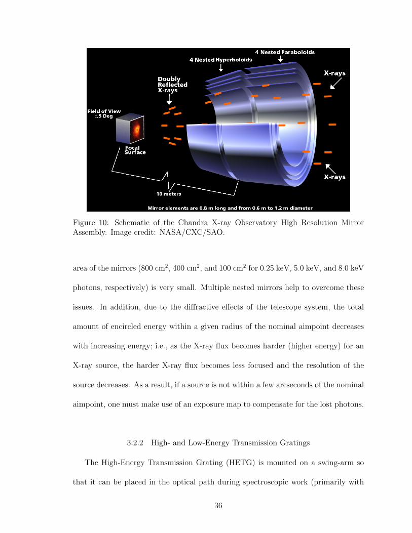
3.2.1 The High Resolution Mirror Assembly
The Chandra X-ray Observatory’s telescope consists of four pairs of nested iridium-
coated mirrors (Fig. 10) known as the High Resolution Mirror Assembly (HRMA).
The mirrors of an X-ray telescope are cylindrical in shape, and Chandra’s mirrors
have diameters that range from 0.65 to 1.23 meters. A spherical mirror, such as
that found in an optical telescope, would be unable to reflect and focus X-ray pho-
tons since X-ray wavelengths are on the order of the size of the atomic/molecular
spacing of the material that makes up the mirror; i.e., the photons would typically
pass through the mirror. To overcome this problem, mirrors make use of “grazing
incidence” in which the surfaces of the mirrors are nearly (within a couple of degrees
of) parallel to the path of the incoming X-ray photons. The photons are first in-
tercepted by four nested mirrors that have a slight parabolic curvature. Afterwards,
the photons are intercepted by a second set of mirrors, located behind the first set,
which have a slight hyperbolic curvature. In e↵ect, these mirrors gradually alter the
trajectory of the photons, requiring the telescope to have a long focal length. As a
result, the detectors have to be placed a large distance from the mirror assembly –
the distance from the Central Aperture Plate (CAP), which separates the parabolic
and hyperbolic mirrors of Chandra, to the focal point of the HRMA is 10.23 meters.
As with all telescopes, light gathering power and resolution are two of the major
design concerns. How e↵ectively the mirrors are able to reflect and focus incoming X-
ray photons depends on the incoming X-ray photon energy as well as the grazing angle
of the mirrors. Due to the cylindrical shape of Chandra’s mirrors, the overall e↵ective
35
Figure 10: Schematic of the Chandra X-ray Observatory High Resolution MirrorAssembly. Image credit: NASA/CXC/SAO.
area of the mirrors (800 cm2, 400 cm2, and 100 cm2 for 0.25 keV, 5.0 keV, and 8.0 keV
photons, respectively) is very small. Multiple nested mirrors help to overcome these
issues. In addition, due to the di↵ractive e↵ects of the telescope system, the total
amount of encircled energy within a given radius of the nominal aimpoint decreases
with increasing energy; i.e., as the X-ray flux becomes harder (higher energy) for an
X-ray source, the harder X-ray flux becomes less focused and the resolution of the
source decreases. As a result, if a source is not within a few arcseconds of the nominal
aimpoint, one must make use of an exposure map to compensate for the lost photons.
3.2.2 High- and Low-Energy Transmission Gratings
The High-Energy Transmission Grating (HETG) is mounted on a swing-arm so
that it can be placed in the optical path during spectroscopic work (primarily with
36
one set of ACIS CCDs) and later retracted during imaging observations. The HETG
(Fig. 11) is composed of two sets of gratings, with each set employing a di↵erent
grating spacing. One set comprises the Medium-Energy Gratings (MEG), which are
used in conjunction with the outer two pairs of mirrors and deal with the lower-
energy (0.4–5.0 keV) X-ray photons, while the other set comprises the High-Energy
Gratings (HEG), which are used in conjunction with the inner two mirror sets that
focus the higher-energy (0.8–10.0 keV) X-rays. The MEG and HEG systems are
composed of 336 individual gratings (144 HEG and 192 MEG) arranged on the HETG
Support Structure (HESS), which places them in proper position behind the HRMA.
The gratings themselves are composed of gold bars electroplated onto a polyimide
substrate, with the bars and corresponding spacings roughly 0.1µm for the HEG
and 0.2µm for the MEG. The rulings of the two sets of gratings are angled ⇠10
degrees to one another so that the medium- and high-energy spectra are separated
from one another. This results in the dispersed X-ray spectrum appearing as an
“X”. Due to multiple gratings needing to focus dispersed spectra onto a single focal
plane, the gratings are arranged in several planes coinciding with the Rowland circle
geometry while the detectors are placed on the opposite portion of the Rowland circle
to intercept the focused spectra.
The Low-Energy Transmission Grating (LETG) is mounted on another swing-arm
and operates in a similar manner to the HETG. The LETG is used primarily with the
HRC-S array (energy range is 0.07 keV–10.0 keV), though it can be used with ACIS-S
(energy range is 0.2–10 keV) with reduced quantum e�ciency. Much like the HETG,
the LETG gratings are mounted on a circular support structure, in this case known
37
!
!
!
Op
tica
l A
xis
On
-ax
is d
etec
tor
loca
tio
n
Det
ecto
r o
ffse
t to
Ro
wla
nd
fo
cus
On
-ax
is
gra
tin
g l
oca
tio
n
Ro
wla
nd
Cir
cle
Dis
per
sio
n d
irec
tio
n
X-r
ay
s
Gra
tin
g f
ace
ts
Cro
ss-d
isp
ersi
on
dir
ecto
n
Ima
gin
g
focu
s
Ro
wla
nd
focu
s
To
p V
iew
Sid
e V
iew
Figure
11:Schem
atic
oftheHighEnergy
Transm
ission
Gratingview
edfrom
face-on(top
-left)
andfrom
theside(bottom-left).
TheRow
landgeom
etry
ofthegratings
anddetectorplacementisshow
nin
therigh
tpan
el.Im
agecredits:
NASA/C
XC/S
AO.
38
as the Grating Element Support Structure (GESS), which places the gratings behind
the HRMA when in use. The GESS supports a system of 180 grating modules, each
of which has three grating facets that each contain 80 grating elements. In the case of
LETG, the grating elements are triangular in shape and are composed of individual
fine gold wires supported by coarser gold wires. Due to the triangular shape of the
coarse support structure, the dispersed spectrum of an X-ray target is star-shaped at
zeroth-order.
3.2.3 HRC
The High Resolution Camera (HRC) is one of two primary imaging instruments
on the integrated Science Instrument Module (SIM) of Chandra. This camera is an
imaging-optimized microchannel plate (MCP) detector (as opposed to the traditional
CCD detector). The HRC, like ACIS, is composed of two sets of detectors. The
HRC-I has the largest field of view of any of the science instruments (300 by 300), and
is optimized for imaging. HRC-S is optimized for spectroscopic work, has a field of
view of 60 by 300, and is used in conjunction with the LETG.
A MCP works on the basis of photoemission. The HRC consists of two MCPs,
each with millions of angled channels that are on the order of 10 microns in diameter.
As an incoming X-ray photon intercepts the MCP, the photon enters a microchannel
and, due to the angle of the channels, strikes the channel wall, which results in the
ejection of an electron. Due to the bias charge between the two plates, the electron
is accelerated down the channel, striking the wall again and releasing more electrons.
This cascade e↵ect continues through the channel, and a shower of several million
39
electrons eventually exits the output microchannel plate where they are intercepted
by an array of detectors that record both the position and charge of an incoming
signal. As multiple photons strike the MCP and the resulting electron showers are
recorded by the position-charge detectors, an image is built up.
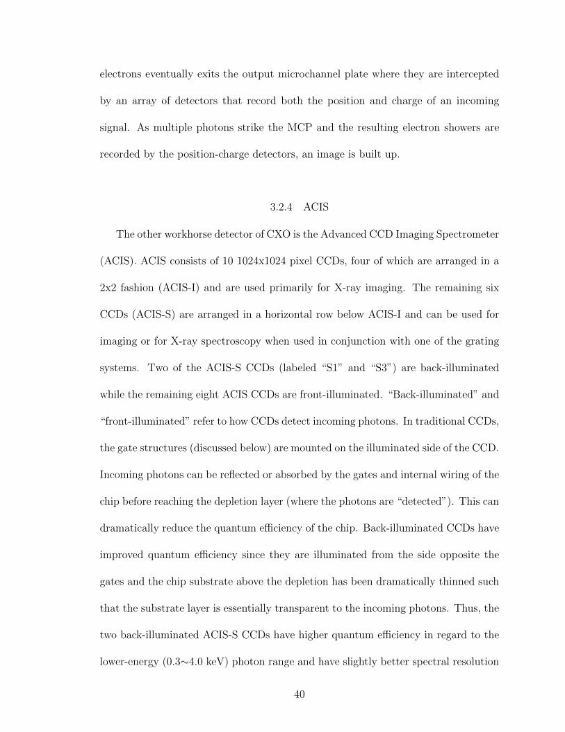
3.2.4 ACIS
The other workhorse detector of CXO is the Advanced CCD Imaging Spectrometer
(ACIS). ACIS consists of 10 1024x1024 pixel CCDs, four of which are arranged in a
2x2 fashion (ACIS-I) and are used primarily for X-ray imaging. The remaining six
CCDs (ACIS-S) are arranged in a horizontal row below ACIS-I and can be used for
imaging or for X-ray spectroscopy when used in conjunction with one of the grating
systems. Two of the ACIS-S CCDs (labeled “S1” and “S3”) are back-illuminated
while the remaining eight ACIS CCDs are front-illuminated. “Back-illuminated” and
“front-illuminated” refer to how CCDs detect incoming photons. In traditional CCDs,
the gate structures (discussed below) are mounted on the illuminated side of the CCD.
Incoming photons can be reflected or absorbed by the gates and internal wiring of the
chip before reaching the depletion layer (where the photons are “detected”). This can
dramatically reduce the quantum e�ciency of the chip. Back-illuminated CCDs have
improved quantum e�ciency since they are illuminated from the side opposite the
gates and the chip substrate above the depletion has been dramatically thinned such
that the substrate layer is essentially transparent to the incoming photons. Thus, the
two back-illuminated ACIS-S CCDs have higher quantum e�ciency in regard to the
lower-energy (0.3⇠4.0 keV) photon range and have slightly better spectral resolution
40
than the front-illuminated CCDs.
Each of the 10 ACIS CCDs has square pixels 0.4900 on a side, giving each CCD
a field of view of 8.30. The total field of view is 16.90 by 16.90 for ACIS-I and 8.30
by 50.60 for ACIS-S. A maximum of six CCDs may be used simultaneously during
an observation. A typical configuration uses all six of the ACIS-S CCDs or all four
ACIS-I CCDs along with the S2 and S3 CCDs (either to maximize the imaging area
for spatially extended X-ray sources or to increase the likelihood of serendipitous
observations of other X-ray events).
When an X-ray photon (with an energy of at least 3.7 eV) strikes the (mostly)
silicon CCD and is absorbed, electrons are liberated. The number of ejected electrons
depends upon the energy of the incident X-ray photon. Due to the removal of an
electron from a silicon atom, a net positive charge – a “hole” – is left behind. The
freed electrons are then confined close to the interaction site via an electric field so
as not to recombine with the holes. After an exposure, the confined charges are
then transferred via “gate structures,” each of which consists of three electrodes that
e↵ectively transfer confined charge from one pixel to another by rapidly varying the
voltages in the electrodes. The gates are also what actually define the pixel boundaries
in the CCD. When the transferred charge reaches the edge of the CCD, the charge
is then transferred to a serial readout that then transfers each pixel charge to a local
processor to determine the position and amplitude of any detected X-rays. Each full
frame exposure lasts 3.2 seconds, e↵ectively giving ACIS a cadence of ⇠3.2 seconds.
As opposed to a typical observation with an optical CCD where the user only sees a
total flux in one filter after an entire observation, the high candence of ACIS allows
41
one to e↵ectively determine the energy of each incoming photon and its corresponding
time of arrival. With the e↵ective energy and arrival time of each individual X-ray
photon recorded, one can build up a crude spectrum as well as a light curve of an
X-ray target; however, additional processing is required for high-flux X-ray sources
that generate “pile-up,” i.e., multiple photons can strike a single part of the CCD
during the 3.2 second frame exposure and mimic the signal of a single, higher-energy
photon.
3.2.5 Other Instruments of Note
Chandra is also equipped with an 11.2 cm Ritchey-Chretien optical telescope and
CCD system mounted to the front of the observatory, which is part of the aspect con-
trol system known as the Aspect Camera Assembly (ACA). The primary function of
the ACA is to monitor a fiducial LED system mounted around the Science Instrument
Module (SIM). The system can also monitor up to five bright stars while simultane-
ously monitoring the fiducial LED system, providing possible optical monitoring of
X-ray targets during an observation.
3.3 From the Telescope to Science Results -CXO Data Reduction
After the raw X-ray data are downloaded from the Chandra X-ray Observatory,
they go through a standard data processing pipeline, carried out by the Chandra X-
ray Center (CXC), in order to begin standard calibration of the raw data and ensure
scientifically usable results. The processing pipeline goes through several stages,
or“levels,” in which various calibrations are applied. Afterward, the end products go
42
through “Verification and Validation” by CXC scientists to ensure the data quality
and investigate any anomalies. Once the calibrated data are ready, the user then
employs data reduction software to extract data from the science files.
The Chandra Interactive Analysis of Observations (CIAO) software was written to
facilitate the analysis of Chandra X-ray data as well as data from other X-ray missions.
This software allows the user to further reduce the data products to his/her individual
scientific needs. In order to generate the final reduced data file, CIAO makes use of
several data products that are produced via the CXC calibration pipeline. Numerous
data files are available if the end user needs to re-reduce the final pipeline products,
but the standard files needed are:
• Observation Fits File – This is the main file which contains all of the observation
data (i.e., target and background data) that will be extracted and used to create
X-ray spectra for analysis.
• Aspect Solution File – This file contains telemetry data concerning the orienta-
tion of the telescope throughout an observation. This file is used in combination
with the events data file to determine the precise celestial position associated
with a detected X-ray event. During an observation, Chandra is dithered, i.e.,
the spacecraft’s aimpoint does not remain fixed throughout the observation but
rather follows a Lissajous pattern. The main purpose of dithering is to smooth
out pixel-to-pixel variations in the detectors, and the aspect solution file ac-
counts for this motion.
• Bad Pixels File – As the name suggests, this file contains a list of known bad
43
pixels or pixel columns.
• Parameter Block File – This file contains information concerning how long each
pixel of the given chip was exposed before being read out.
• Dead Area Correction Files – This standard set of calibration files is used to
account for cosmic rays striking an ACIS CCD and rendering portions of it
unusable during an entire frame.
• Mask File – This telemetry file denotes which parts of a CCD were active
during an observation, and, thus, from which pixels are usable to extract events
data. The active “window” of a CCD is determined by factors such as the pixel
clocking mode.
With these calibration files, one of the typical routines used for extracting point-
source spectra is the CIAO routine specextract (or psextract in previous versions of
CIAO). This program utilizes several tools built into CIAO to apply the calibration
files to the events file and produce reduced data products such as:
• Response Matrix File (RMF) – This file contains information concerning the
detector response; i.e., it correlates the response of the detector with the pulse
height read out by the CCD in order to determine the properties of the incoming
photons, such as the photon energies.
• Ancillary Response File (ARF) – This file contains the e↵ective area versus
energy for the detector and telescope configuration of a given observation.
44
• Pulse Height Amplitude (PHA) or Pulse Invariant (PI) Files – This FITS file
contains tabulated data regarding X-ray events detected during an observation.
Mainly pertinent to the end-user is the “data” block of the file, which includes
the detector channels, their corresponding energies, event count rates and the
associated count rate errors, and the group that each channel belongs to in
instances when the data are binned. PI files are essentially PHA files that
have the RMF applied, i.e., the pulse-height amplitude has been converted to
a corresponding energy using the detector response stored in the RMF file. A
background PI file is created in addition to a source (target) PI file to allow
the spectral modeling software to estimate the source spectrum contamination
from background X-ray flux. One also typically uses CIAO to create a back-
ground light curve to determine if the X-ray background underwent any flaring
during the observation, which could drastically a↵ect the analysis of the target
spectrum if not properly accounted for.
Once the spectrum files and their corresponding RMF and ARF files are created,
spectral modeling can begin. The typical X-ray analysis packages used to model
CXO X-ray data are XSPEC, X-ray spectral modeling software produced by the
High Energy Astrophysics Science Archive Research Center (HEASARC) (Arnaud,
1996), or Sherpa, CIAO’s built-in modeling and fitting software package (Freeman et
al., 2001). These packages are mission-independent, meaning that even though they
were written for analyzing CXO data they are also capable of modeling data from
other X-ray missions such as XMM-Newton and Suzaku. These packages have a great
45
deal of built-in flexibility in how they can be used to model data. For example, one
can model a single spectrum with a single model, simultaneously fit multiple spectra
to the same model, or simultaneously fit multiple spectra to a single model but allow
some parameters to vary per spectrum.
46
CHAPTER IV
X-RAY PRODUCTION BY V1647 ORI DURING OPTICAL OUTBURSTS
In this chapter, I present a manuscript that was published in the Astrophysical
Journal in November 2011, which deals with analysis of the X-ray observations ob-
tained of the young, erupting star V1647 Ori during its 2008 optical outburst. This
paper, in which I am first author, is listed in the references of this dissertation as
Teets et al. (2011).
4.1 Introduction
The young stellar object (YSO) V1647 Ori was first noted to be an erupting
source when it brightened suddenly in November 2003, illuminating a new nebula
now known as McNeil’s Nebula. This deeply embedded, low-mass YSO is typically
considered to be an EX Lupi-type object (an “EXor”) though it shares some spectral
characteristics with FU Orionis (Vacca et al., 2004), the prototype of a similar class of
erupting pre-main sequence (PMS) stars (“FUors”). EXors are observed to brighten
irregularly at optical wavelengths up to several times per decade; these outbursts
persist for weeks to months (Herbig, 2001). FUors are YSOs that erupt less often than
EXors, perhaps only once per century, and fade much more slowly, i.e., on timescales
of years to decades (Herbig, 1977). The general consensus is that these eruptions
are the result of massive accretion events that occur irregularly as young protostars
grow; such accretion episodes may be the primary process through which young stars
47
accrete most of their mass (Hartmann & Kenyon, 1996). The mechanisms underlying
EXor and FUor outbursts remain very poorly understood; however, models generally
invoke the rapid onset of disk instabilities that lead to sudden inward migration of
the inner disk truncation radius and dramatic changes in the star/disk magnetic field
configuration (e.g., Zhu et al. (2009); Konigl et al. (2011)).
Soft X-ray (⇠0.3 keV) generation via shock-heating of plasma at the bases of PMS
accretion streams has been proposed for some objects from X-ray grating observations
(see review by Gudel & Naze, 2009) using plasma diagnostics based on helium-like
ions (see review by Porquet et al., 2010), a prime example being TW Hydrae (Kastner
et al., 2002; Brickhouse et al., 2010). On the other hand, studies such as the Chandra
Orion Ultradeep Project (COUP) indicate that coronal activity, and not accretion, is
likely the primary production mechanism for the harder X-rays that are characteristic
of most pre-main sequence stars (Preibisch et al., 2005; Stassun et al., 2006). Debate
still lingers as to the primary X-ray generation mechanism in YSOs during optical
outbursts.
Since 2003, V1647 Ori has been observed to undergo two distinct outbursts that
have been detected in the optical and near-infrared (McNeil, 2003; Itagaki et al.,
2008) as well as at X-ray wavelengths (Kastner et al., 2004, 2006; Grosso et al., 2005;
Grosso, 2006; Hamaguchi et al., 2010). The magnitudes and timescales for brightening
and fading displayed by V1647 Ori do not match those of EXors. Furthermore, the
duration of the initial outburst was shorter than those of FUors (Kastner et al., 2006;
Aspin, Beck, & Reipurth, 2008). However, spectroscopic data do show signatures of
accretion, such as strong H↵ and Br� emission (Reipurth & Aspin, 2004; Brittain et
48
al., 2010), confirming that the eruptions of V1647 Ori do resemble those of FUors
and EXors.
V1647 Ori has been observed in X-rays before and during both of the eruptions (as
well as after the first of the two eruptions) detected in the optical/near-infrared since
2003. Although other FUor- or EXor-like YSOs have been observed in X-rays (V1118
Ori (Audard et al., 2010); EX Lup (Grosso et al., 2010); Z CMa (Stelzer et al., 2009);
FU Ori (Skinner et al., 2006); V1735 Cyg (Skinner et al., 2009)), V1647 Ori is the only
eruptive YSO to undergo such extensive X-ray monitoring. During the 2003 eruption,
the sudden rise in flux and subsequent decline in both the optical and near-infrared
correlated strongly with a sharp increase and then decline in the X-ray flux, which
suggests a common origin (Kastner et al., 2004, 2006). In this paper, we present and
analyze X-ray spectra obtained with the Chandra X-ray Observatory (CXO) during
the 2008–2009 outburst. In §4.2, we describe the observations and data reduction. In
§4.3, we examine the trends and patterns seen in the X-ray emission from V1647 Ori
over the past two outbursts, present modeling results for each of the five recent CXO
observations, and compare these results to those obtained from previous (2003–2005)
CXO and XMM-Newton observations. Finally, in §4.4 we discuss the implications
of the results, and we argue that the measured properties of the X-ray emitting
plasma are best understood within the framework of the accretion-generated X-ray
hypothesis.
49
4.2 Observations & Data Reduction
Observations of V1647 Ori made with the Chandra X-ray Observatory (CXO)
were triggered in 2008 September with a 20 ks observation (CXO Cycle 10, PI: D.
Weintraub, ObsID 9915), after V1647 Ori was reported to have undergone a new op-
tical outburst between early 2008 January and late 2008 August (Itagaki et al., 2008).
Subsequent 20 ks observations were initiated in 2009 January and April (ObsIDs 9916
and 9917, PI: D. Weintraub). In addition, in 2008 November, two observations (Ob-
sIDs 10763 and 8585; PI: N. Calvet) were made of the NGC 2068/2071 region that
serendipitously included V1647 Ori. Together, these five CXO pointings yield an ex-
tended sequence of observations of this source over a seven-month period immediately
following the onset of the optical outburst in 2008.
Fortuitously, a field of view that includes V1647 Ori was observed in 2002 Novem-
ber, a full year before the start of the 2003 outburst (Simon et al., 2004); subsequent
CXO observations targeting V1647 Ori were obtained in 2004 March and April, 2005
August and December, and 2006 May and August (Kastner et al., 2004, 2006). In
addition, targeted XMM-Newton observations were obtained in 2004 April (Grosso et
al., 2005) and 2005 March (Grosso, 2006), and a targeted Suzaku observation was ob-
tained in 2008 October (Hamaguchi et al., 2010). The 2004–2006 observations cover
a two-year period during which V1647 Ori more or less faded steadily from a strong
YSO X-ray source into a very faint one, albeit with large X-ray flux variability. For
direct comparison with our analysis of the 2008–2009 epoch datasets, we have re-
reduced and analyzed all of the 2002–2006 CXO datasets, using the same techniques
50
and software packages that we have used for the latest (2008–2009) datasets.
For all Chandra observations, the Advanced CCD Imaging Spectrometer (ACIS)
was used in one of two imaging configurations. ACIS detectors have a pixel size of
0.4900 and each ACIS-I and ACIS-S CCD has a field of view of 8.30 ⇥ 8.30. CXO/ACIS
has significant sensitivity over the energy range 0.3–10 keV, with the soft (<1 keV)
X-ray sensitivity dependent on whether a back-illuminated or front-illuminated CCD
serves as the detector (see below). The CIAO v4.1 software package and CALDB
v4.1.0–4.1.4 calibration files were used to reduce the data and extract pulse-invariant
(PI) spectra. Observation details are given in Table 1. To compare X-ray luminosities
from 2008–2009 with those obtained from previous observations, source spectra were
extracted from 2.500 radius regions (making sure the aperture was positioned so as to
encompass as many source photons as possible, even when V1647 Ori is 40 o↵-axis)
while background spectra were extracted from regions near but beyond 2.500 from the
target, on the same chip, using 2000 outer radius extraction apertures. Inspection of
background light curves reveals background levels to be fairly constant with no evi-
dence of large fluctuations, such as flares, occurring during the observations. Spectra
were also re-extracted from previous Chandra observations using the same apertures
to ensure that direct comparisons of results from di↵erent observation epochs could
be performed reliably. For observations in which the primary target was not V1647
Ori (ObsIDs 2539, 10763, and 8585), exposure maps were generated to investigate
o↵-axis position e↵ects. In all three of these observations, the net count and mean
count rate corrections due to o↵-axis source positions were insignificant, on the order
of a few percent. The resultant spectral data points of the five recent observations
51
were grouped into energy bins with a minimum of five counts per bin before spectral
modeling was done. The count rates were high enough and durations long enough
for each of the 2008–2009 observations that this bin size yielded PI spectra with
good statistics. For the 2002–2006 observations, we employed single-count-minimum
binning for very low-count observations and five-count-minimum binning for higher-
count observations so as to yield spectra suitable for modeling. Because no events
with energies less than 0.5 keV and few events with energies greater than 8.0 keV
were detected from V1647 Ori, we limited our modeling to the 0.5–8.0 keV energy
range.
52
Tab
le1.
2002–2009ACIS
Observationsof
V1647
Ori.
ObsI
DO
bse
rvat
ion
JD
AC
ISE
xpos
ure
Net
Cou
nts
Mea
nC
ount
Med
ian
Phot
onM
ean
Har
dnes
saH
ardnes
sR
atio
b
Dat
eC
hip
(ks)
(0.5
–8.0
keV
)R
ate
(ks�
1)
Ener
gy(k
eV)
Rat
ioof
Tot
alC
ounts
2539
c20
02N
ov14
2452
593
S2
62.8
170.
3±
0.1
2.0±
0.3
�0.
34±
0.31
�0.
28±
0.28
5307
d20
04M
ar07
2453
072
S3
5.5
6411
.7±
1.5
3.6±
0.3
0.46
±0.
150.
45±
0.14
5308
d20
04M
ar22
2453
087
S3
4.9
122.
5±
0.8
2.0±
0.5
�0.
45±
0.33
�0.
46±
0.33
5382
2005
Apr
1124
5347
2I3
18.2
864.
8±
0.5
3.5±
0.1
0.51
±0.
190.
46±
0.12
5383
2005
Aug
2724
5361
0I3
19.9
180.
9±
0.2
3.0±
0.8
0.01
±0.
290.
34±
0.25
5384
2005
Dec
0924
5371
4I3
19.7
20.
1±
0.1
2.2±
1.1
0.0±
0.20
�0.
07±
0.92
6413
2005
Dec
1424
5371
9I3
18.1
40.
2±
0.1
1.7±
0.3
�0.
36±
0.26
�1.
0±
0.75
6414
2006
May
0124
5385
7I3
21.6
30.
1±
0.1
1.3±
0.3
0.09
±0.
230.
07±
0.92
6415
2006
Aug
0724
5395
5I3
20.5
40.
2±
0.1
2.4±
0.4
�0.
27±
0.21
�1.
0±
0.73
9915
2008
Sep
1824
5472
8I3
19.9
466
23.6
±1.
13.
5±
0.1
0.36
±0.
070.
37±
0.05
1076
3c20
08N
ov27
2454
798
I219
.721
711
.0±
0.7
3.9±
0.1
0.65
±0.
090.
64±
0.08
8585
c20
08N
ov28
2454
799
I228
.516
05.
8±
0.4
3.4±
0.1
0.40
±0.
100.
43±
0.09
9916
2009
Jan
2324
5485
5I3
18.4
245
13.6
±0.
93.
7±
0.2
0.41
±0.
080.
43±
0.07
9917
2009
Apr
2124
5494
3I3
29.8
260
8.8±
0.5
3.5±
0.2
0.28
±0.
080.
37±
0.07
aA
vera
geof
har
dnes
sra
tios
com
pute
dfr
om2
ks
ligh
tcu
rve
dat
abin
s(O
bsI
D25
39use
s10
ks
ligh
tcu
rve
dat
abin
s).
bH
ardnes
sra
tio
com
pute
dusi
ng
the
tota
lnum
ber
sof
har
dan
dso
ftX
-ray
phot
ons
from
the
entire
obse
rvat
ion.
cV
1647
Ori
was
not
the
targ
etof
the
obse
rvat
ion,an
dgi
ven
valu
eshav
ebee
nad
just
edto
com
pen
sate
for
the
40o↵
-axis
pos
itio
nof
V16
47O
ri.
Expos
ure
map
sin
dic
ated
net
counts
and
mea
nco
unt
rate
sfo
rO
bsI
D25
39sh
ould
be
incr
ease
dby
8%w
hile
thos
efo
rO
bsI
Ds
1076
3an
d85
85re
quir
eda
3%in
crea
se.
dT
he
bac
k-illum
inat
edA
CIS
-S3
CC
Dis
mor
ese
nsi
tive
toX
-ray
sfr
ompla
sma
inth
ete
mper
ature
regi
me
char
acte
rist
icof
V16
47O
rith
anar
eth
efr
ont-
illu
min
ated
AC
ISC
CD
s.Val
ues
dis
pla
yed
for
net
counts
and
mea
nco
unt
rate
s,an
dth
eir
asso
ciat
eder
rors
,fo
rO
bsI
Ds
5307
and
5308
hav
ebee
nad
just
eddow
nw
ard
by
10%
,bas
edon
spec
tral
sim
ula
tion
sin
order
tom
ake
net
counts
and
mea
nco
unt
rate
sdir
ectl
yco
mpar
able
bet
wee
nal
lch
ips.
Not
e.—
All
erro
rsar
e1�.
The
net
counts
for
each
obse
rvat
ion
are
the
tota
lnum
ber
ofco
unts
wit
hin
the
0.5–
8.0
keV
range
.M
edia
nphot
onen
ergy
unce
rtai
nti
esw
ere
calc
ula
ted
via
the
hal
f-sa
mple
met
hod
use
din
Kas
tner
etal
.(2
006)
.M
ean
count
rate
sw
ere
det
erm
ined
by
div
idin
gth
enet
counts
by
expos
ure
tim
es.
Unce
rtai
nti
esfo
rm
ean
count
rate
san
dhar
dnes
sra
tios
ofto
talco
unts
follow
Poi
sson
stat
isti
cs.
The
unce
rtai
nty
for
the
har
dnes
sra
tio
ofth
eto
talco
unts
for
ObsI
D53
84co
uld
not
be
calc
ula
ted
due
toth
eev
endis
trib
ution
ofth
eve
rylo
wnum
ber
ofco
unts
53
Since V1647 Ori was imaged with both front- and back-illuminated CCDs in the
exposure sequence under analysis, we generated synthetic spectra and convolved these
spectra with the instrument responses to determine whether mean, broadband (0.5–
8.0 keV) count rates were directly comparable for all observations of V1647 Ori. The
simulations (Table 2) showed that, for the plasma temperature regimes considered
here, the back-illuminated S3 CCD is ⇠10% more sensitive to incoming flux than
the front-illuminated ACIS-I CCDs. Net counts and mean count rates in the energy
range 0.5–8.0 keV (Table 1) were therefore adjusted downward accordingly for the
two observations (ObsIDs 5307 and 5308) that used the S3 CCD in order to remove
this sensitivity bias.
54
Tab
le2.
Com
parison
ofSim
ulatedFront-an
dBack-Illuminated
ACIS
Chip
Exp
osures
Pla
sma
S3/
I3S3
I3H
RTem
per
ature
(kev
)C
ount
Rat
ioH
RH
RD
i↵er
ence
21.
210.
020.
120.
105
1.14
0.30
0.38
0.08
71.
110.
400.
480.
08
Not
e.—
Net
count
and
har
dnes
sra
tio
(of
tota
lco
unt
s)co
mpar
ison
sfo
rsi
mula
ted
spec
tra
conv
olve
dw
ith
inst
rum
entre
spon
sesfr
omO
bsI
Ds53
07an
d99
15,w
hic
huse
dth
ebac
k-illu
min
ated
S3
CC
Dan
dfr
ont-
illu
min
ated
I3C
CD
,re
spec
tive
ly.
Eac
hof
the
1-ks
spec
tra
wer
esi
mula
ted
usi
ng
thefakeit
com
man
din
XSP
EC
wit
hth
ein
terv
enin
ghy
dro
gen
colu
mn
den
sity
and
chem
ical
abundan
cefixe
dat
4.0
⇥10
22cm
�2
and
0.8
sola
r,re
spec
tive
ly.
The
fron
t-illu
min
ated
chip
det
ects
rough
ly85
%of
the
net
count
sof
the
bac
k-illu
min
ated
chip
,w
ith
agr
eate
rdro
pin
sensi
tivi
tyfo
rso
ftve
rsus
har
dX
-ray
s.
55
4.3 Results
4.3.1 Short-Term and Long-Term Variability
We calculated the median photon energies, mean count rates, and mean hardness
ratios for all 14 CXO observations of V1647 Ori. These results are reported in Table 1.
In calculating the hardness ratios, the hard (H) X-rays are defined as those in the
range from 2.8 to 8.0 keV and the soft (S) X-rays as those with energies from 0.5
to 2.8 keV (Grosso et al., 2005). The hardness ratio is then HR = (H-S)/(H+S),
such that negative values of HR indicate softer spectra, and positive values indicate
harder spectra. The recalculated values and error ranges of the mean count rates and
median photon energies for the 2004–2006 observations di↵er only marginally from
those reported by Kastner et al. (2006). With data from only three epochs in hand,
Kastner et al. (2004) reported that the X-ray flux brightened and hardened during the
outburst (2002 November 14 to 2004 March 07) and then quickly faded and softened
post-outburst (2004 March 07 to 2004 March 22). With data from additional epochs
available, however, Kastner et al. (2006) reinterpreted the late 2004 March data as a
short-term downward fluctuation, not as a quick end to the original outburst. They
interpret the observed pattern of changes in the median photon energy as evidence
that the X-ray spectrum hardened during outburst, remained somewhat hard for at
least one year, and then softened after 2005 August 27 as both the optical and X-ray
flux from V1647 Ori returned to pre-outburst levels. The results obtained here (for
hardness ratio) confirm this general trend. This hardening and softening (the mean
hardness ratios (with 1� uncertainties) changed from �0.34 ± 0.31 (soft) to +0.46
56
± 0.15 (hard) and back to �0.45 ± 0.33 (very soft) over the course of three years,
from 2002 November through 2005 December) took place over a timescale of months,
with V1647 Ori remaining near peak outburst X-ray luminosity and hardness for
more than one year - with the notable exception of the 2004 March 22 data. V1647
Ori likely remained in its soft X-ray, low X-ray luminosity phase for almost three
years, from late 2005 until its latest optical outburst in 2008 August. The five CXO
observations covering the interval from 2008 September through 2009 April all show
V1647 Ori in a hard X-ray, high X-ray luminosity state. As was the case during the
2002–2006 observations, the source remained near peak X-ray luminosity for at least
seven months (Fig. 22, figure to be discussed in Section 4.4). As of 2009 December
18, V1647 Ori appeared to still be in an outburst phase with J-, H-, and K-band
photometric magnitudes near values measured at the brightest phase of outburst
during 2008 September (Venkat & Anandarao, 2009). Thus, it appears that V1647
Ori remained near peak luminosity for at least one year.4
X-ray light curves and hardness ratios as a function of time were extracted for each
observation to examine the properties of any possible short-term X-ray variability. In
particular, these time series data permit us to investigate whether the trends in X-ray
flux and hardness ratio seen in 2002–2006 were repeated during the recent outburst
that began around 2008 August. The extracted X-ray light curves and hardness
ratio time series for six of the nine observations from 2002–2006 are presented in
Figure 12. X-ray light curves and hardness ratio curves for the five 2008–2009 Chandra
observations are presented in Figures 13–17, which show (from top to bottom) the
4As of submission of this paper, the outburst appears to be ongoing.
57
overall X-ray light curve, the soft (0.5–2.8 keV) light curve, the hard (2.8–8.0 keV)
light curve, and the hardness ratio time series. Energy ranges for the soft and hard
X-ray bands follow those defined in Grosso et al. (2005), and plotted uncertainties in
mean hardness ratios and count rates are 1�.
58
2002 N
ove
mber
14
Ela
pse
d O
bse
rva
tion
Tim
e (
ks)
010
20
30
40
50
60
70
Count Rate (cts/s)
0
0.0
001
0.0
002
0.0
003
0.0
004
0.0
005
0.0
006
Hardness Ratio (H!S/H+S)
!2
!101
2004 M
arc
h 0
7
Ela
pse
d O
bse
rva
tion
Tim
e (
ks)
02
46
Count Rate (cts/s)
0.0
06
0.0
08
0.0
1
0.0
12
0.0
14
0.0
16
Hardness Ratio (H!S/H+S)
0
0.2
0.4
0.6
0.81
2004 M
arc
h 2
2
Ela
pse
d O
bse
rva
tion
Tim
e (
ks)
02
46
Count Rate (cts/s)
0.0
01
0.0
02
0.0
03
0.0
04
0.0
05
Hardness Ratio (H!S/H+S)
!2
!101
2005 A
pril 1
1
Ela
pse
d O
bse
rva
tion
Tim
e (
ks)
05
10
15
20
Count Rate (cts/s)
0
0.0
02
0.0
04
0.0
06
0.0
08
0.0
1
0.0
12
Hardness Ratio (H!S/H+S)
!0.50
0.51
1.5
2005 A
ugust
27
Ela
pse
d O
bse
rva
tion
Tim
e (
ks)
05
10
15
20
Count Rate (cts/s)
0
0.0
01
0.0
02
0.0
03
Hardness Ratio (H!S/H+S)
!1.5!1
!0.50
0.51
1.5
2005 D
ece
mber
14
Ela
pse
d O
bse
rva
tion
Tim
e (
ks)
05
10
15
20
Count Rate (cts/s)
0
0.0
002
0.0
004
0.0
006
0.0
008
0.0
01
Hardness Ratio (H!S/H+S)
!1.5!1
!0.50
0.51
Figure
12:Backg
round-subtractedX-ray
ligh
tcurves
for2002-2006ep
ochob
servations.
Tim
ebinsare2ks
foreach
observation
(except2002
Novem
ber
14,whichuses10
ksbinsdueto
thevery
low
count
rate)an
dcontaincounts(0.5–8.0
keV)per
total
timeassociated
witheach
bin,not
thetotaltimeassociated
withtheob
servation.Observationsfor2005
Decem
ber
09,2006
May
01,an
d2006
Augu
st07
donot
detectV1647
Ori,so
theirligh
tcurves
arenot
presented.Uncertaintiesin
meanhardness
ratios
andcount
ratesare1�
.
59
2008 September 18
Elapsed Observation Time (ks)
0 5 10 15 20
Count R
ate
(ct
s/s)
0
0.01
0.02
0.03C
ount R
ate
(ct
s/s)
0
0.01
0.02
0.03
Count R
ate
(ct
s/s)
0
0.01
0.02
0.03
Hard
ness
Ratio
(H
!S
/ H
+S
)
!0.5
0
0.5
1
Energ
y Range (2
.8 !
8.0
keV
)E
nerg
y Range (0
.5 !
2.8
keV
)E
nerg
y Range (0
.5 !
8.0
keV
)
Figure 13: X-ray light curves and hardness ratio of V1647 Ori during observation9915. The top panel light curve covers the 0.5–8.0 keV energy range, the secondpanel down spans the lower energy range of 0.5–2.8 keV, and the third panel downcovers the higher 2.8–8.0 keV energies. The bottom panel displays the hardness ratiofor each of the bins. Counts were binned into 2 ks bins. Uncertainties in meanhardness ratios and count rates are 1�. Apparent “X-ray bright” time intervals areindicated by the shaded regions in the figure (4–8 ks and 16–20 ks) and in Figures14–17.
60
2008 November 27
Elapsed Observation Time (ks)
0 5 10 15 20
Co
un
t R
ate
(ct
s/s)
0
0.005
0.01
0.015
0.02
Co
un
t R
ate
(ct
s/s)
0
0.005
0.01
0.015
0.02
Co
un
t R
ate
(ct
s/s)
0
0.005
0.01
0.015
0.02
Ha
rdn
ess
Ra
tio (
H!
S /
H+
S)
!0.5
0
0.5
1
1.5
En
erg
y Ra
ng
e (2
.8 !
8.0
keV
)E
ne
rgy R
an
ge
(0.5
! 2
.8 ke
V)
En
erg
y Ra
ng
e (0
.5 !
8.0
keV
)
Figure 14: X-ray light curves and hardness ratio of V1647 Ori during observation10763. See Figure 13 for description of panels. Counts were binned into 2 ks bins.Uncertainties in mean hardness ratios and count rates are 1�. V1647 Ori had aslightly elevated X-ray flux, seen best in the hard X-ray band, from 8–10 ks.
61
2008 November 28
Elapsed Observation Time (ks)
0 10 20 30
Co
un
t R
ate
(ct
s/s)
0
0.005
0.01
0.015
Co
un
t R
ate
(ct
s/s)
0
0.005
0.01
0.015
Co
un
t R
ate
(ct
s/s)
0
0.005
0.01
0.015
Ha
rdn
ess
Ra
tio (
H!
S /
H+
S)
!1
!0.5
0
0.5
1
1.5
En
erg
y Ra
ng
e (2
.8 !
8.0
keV
)E
ne
rgy R
an
ge
(0.5
! 2
.8 ke
V)
En
erg
y Ra
ng
e (0
.5 !
8.0
keV
)
Figure 15: X-ray light curves and hardness ratio of V1647 Ori during observation8585. Counts were binned into 2 ks bins. Uncertainties in mean hardness ratiosand count rates are 1�. The hard and broad-band X-ray light curves show that thehard X-ray flux from V1647 Ori increased sharply at 20 ks into the observation andremained elevated for ⇠10 ks. During this period of elevated X-ray flux, the soft-bandflux remained more or less constant.
62
2009 January 23
Elapsed Observation Time (ks)
0 5 10 15 20
Count R
ate
(ct
s/s)
0
0.01
0.02
0.03
Count R
ate
(ct
s/s)
0
0.01
0.02
0.03
Count R
ate
(ct
s/s)
0
0.01
0.02
0.03
Hard
ness
Ratio
(H
!S
/ H
+S
)
!0.5
0
0.5
1
Energ
y Range (2
.8 !
8.0
keV
)E
nerg
y Range (0
.5 !
2.8
keV
)E
nerg
y Range (0
.5 !
8.0
keV
)
Figure 16: X-ray light curves and hardness ratio of V1647 Ori during observation9916. Counts were binned into 2 ks bins. Uncertainties in mean hardness ratios andcount rates are 1�. The X-ray light curve shows that V1647 Ori began increasing inhard-band and, possibly, soft-band flux about 8 ks into the observation, and the fluxremained elevated for ⇠12 ks.
63
2009 April 21
Elapsed Observation Time (ks)
0 10 20 30
Count R
ate
(ct
s/s)
0
0.01
0.02
0.03
Count R
ate
(ct
s/s)
0
0.01
0.02
0.03
Count R
ate
(ct
s/s)
0
0.01
0.02
0.03
Hard
ness
Ratio
(H
!S
/ H
+S
)
!1
!0.5
0
0.5
1
Energ
y Range (2
.8 !
8.0
keV
)E
nerg
y Range (0
.5 !
2.8
keV
)E
nerg
y Range (0
.5 !
8.0
keV
)
Figure 17: X-ray light curves and hardness ratio of V1647 Ori during observation9917. Counts were binned into 2 ks bins. Uncertainties in mean hardness ratios andcount rates are 1�. V1647 Ori appeared to be in an elevated hard X-ray flux state atthe onset of the observation, with the X-ray count rate remaining elevated for ⇠8 ks.
64
The X-ray count rate for V1647 Ori was intrinsically lower during most of the
2002-2006 observations (the count rate was >5 ks�1 only on 2004 March 07) than in
2008–2009 (the count rate was >5 ks�1 during all five observations). Also, in some
cases like ObsIDs 5307 and 5308 (both from 2004), the observations were on the order
of only a few kiloseconds in duration. The low count rates in most of the 2002–2006
data and the short exposure times in two of these observations make comparisons with
the more recent datasets, in terms of the presence or absence of 2–10 ks timescale
variations, fairly di�cult. However, observations 5382 and 5383, obtained in 2005
April and August, respectively – more than a year after the initial optical outburst
of V1647 Ori in 2003 November – yielded enough counts that we can compare these
two light curves with the more recent observations with some confidence. As seen in
these two light curves from 2005 (Fig. 12, lower-left panel, beginning at ⇠10 ks, and
lower-middle panel, beginning at ⇠5 ks), the X-ray count rate again varied by a factor
of ⇠4 on a timescale of 2–10 ks, a level and duration of short-term variability very
similar to that seen in the more recent (2008–2009) observations. We conclude that
kilosecond-timescale variations are seen in all observations of V1647 Ori in which the
signal is strong enough and the observing window long enough for us to search for such
events, and that the amplitude duty cycle and duration of these few-kilosecond X-ray
variations were stable over the five-year period from 2005 to 2009. Such variability
appears to be part of the normal X-ray pattern for this object, at least when the count
rate is elevated. One therefore needs to interpret the overall flux levels observed during
the 2004 March 07 and 2004 March 22 observations, which, respectively, are only 5.5
ks and 4.9 ks in duration, with caution.
65
The highest measured X-ray mean count rate following the latest (2008) optical
outburst of V1647 Ori is higher (23.6 ks�1; one month post-outburst) than the highest
level (11.7 ks�1; four months post-outburst) observed during its 2003–2005 outburst
(Table 1). In addition, with the exception of the 2004 March 07 observation, the
2008–2009 observations (a period spanning seven months) show V1647 Ori to be
consistently brighter than it was during the 2003–2005 outburst. We find that in
2008–2009 the X-ray spectrum stays relatively hard, as is shown by the median photon
energies, which in 2008–2009 are consistently about twice the energy (3.4 to 3.9 keV)
that was observed before the first eruption (2.0 keV in 2002) and after V1647 Ori had
returned to its quiescent state in late 2005 (1.7 keV). Also, while the mean hardness
ratios were negative both before (2002 November) and after (2005 December) the
first eruption, the mean hardness ratios in 2008–2009 stay consistently around ⇠0.3
or greater.
These results also reveal that V1647 Ori exhibited a very interesting sequence of
changes of state, beginning in 2004 March. V1647 Ori had switched from its elevated
state on 2004 March 07 (11.7 counts ks�1, median photon energy of 3.6 keV, mean
hardness ratio of +0.46) to what appears to be a quiescent state on 2004 March 22 (2.5
cts ks�1, median photon energy of 2.0 keV, �0.45 mean hardness ratio) but then was
again in an elevated state one year later on 2005 April 11 (4.8 cts ks�1, median photon
energy of 3.5 keV, mean hardness ratio of +0.51). Yet by 2005 August 27, V1647
Ori was again returning to quiescence (0.9 cts ks�1, 3.0 keV median photon energy,
+0.01 mean hardness ratio) and by 2005 December was fully back to quiescence.
At least three explanations are plausible for the observed changes we have de-
66
scribed in the X-ray emission from V1647 Ori that occurred between 2004 March 07
and 2004 March 22 and between 2004 March 22 and 2005 April 11. One: the outbursts
generate both hard and soft X-rays; most of the time (2004 March 07 and 2005 April
11), the hard X-ray plasma is dominant in the X-ray spectrum as observed by CXO,
but at certain times (2004 March 22) the soft X-ray plasma component is seen more
clearly. Two: the first major outburst (2003 November through early 2004 March)
had ended, at least in the X-ray regime, after only a few months. By 2005 April,
the source was again in an elevated state and by 2005 August, four months later,
was again returning to quiescence. Three: the 2004 March 22 observation caught
V1647 Ori during a short duration (2–10 ks) quiescent moment during the extended
(months long) outburst phase. However, the XMM-Newton observation obtained on
2004 April 4 showed a low X-ray flux level at the beginning of the observation that is
consistent with the quiescent level observed by CXO that increased in the second part
of the observation (Grosso et al., 2005). Moreover, the supporting evidence from ob-
servations made at optical and near-infrared wavelengths for the first outburst ending
in 2004 mid-March and for a second outburst beginning later that year (explanation
“Two”) is weak, at best. Of the remaining two possibilities, we will argue in §4 that
explanation “One” is more likely.
A comparison of the count rates (Figs. 13–17, top panels) and hardness ratios
(Figs. 13–17, bottom panels) during the ⇠2–10 ks variability periods suggests that
the X-ray spectrum of V1647 Ori may harden as it brightens and soften as the source
fades during these few-kilosecond variations. This appearance of a correlation between
the changing count rate and the changing hardness ratio on a few kilosecond timescale
67
during short-term variability, however, is not consistent. In fact, we find a weak anti-
correlation between these properties (correlation coe�cient = �0.18) on these short
timescales; however, we do find a strong, positive correlation over much longer periods
of time between the X-ray luminosity (calculated in our spectral modeling; see Section
4.3.2) and hardness ratio, as shown in Figure 18. In this figure, the top panels show
the seven-year X-ray luminosity curve of V1647 Ori while the middle panels show
the corresponding hardness ratios with a single, average measurement plotted for
each observation epoch. A more direct demonstration of this correlation is shown in
Figure 19 where we plot the change in mean hardness ratio versus the change in X-ray
luminosity between observations of V1647 Ori. We derive a correlation coe�cient of
0.44 for these two parameters.
68
2002!2006 V1647 Ori Chandra Observations
Julian Date ! 2450000
2750 3000 3250 3500 3750 4000
Lum
inosi
ty (
erg
s s!
1 )
1e+28
1e+29
1e+30
1e+31
Hard
ness
Ratio
(H
!S
/ H
+S
)
!1
!0.5
0
0.5
1
Pla
sma T
em
pera
ture
(ke
V)
0
5
10
15
2003 2004 2005 2006
2008!2009 V1647 Ori Chandra Observations
Julian Date ! 2450000
4700 4750 4800 4850 4900 4950
Lu
min
osi
ty (
erg
s s!
1 )
1e+28
1e+29
1e+30
1e+31
Ha
rdn
ess
Ra
tio (
H!
S /
H+
S)
!1
!0.5
0
0.5
1
Pla
sma
Te
mp
era
ture
(ke
V)
0
5
10
15
Sep 08 Nov 08 Jan 09 Mar 09 May 09
Figure 18: Time series of observed X-ray luminosity (top panels), mean hardness ra-tio (middle panels), and plasma temperature (bottom panels) for V1647 Ori. Crossesrepresent data obtained with ACIS front-illuminated CCDs, and squares representdata obtained with the ACIS back-illuminated S3 CCD. Plotted uncertainties forthe hardness ratios and luminosities represent the 68% confidence interval (1�) andplotted uncertainties for the plasma temperatures represent the 90% confidence inter-val (1.6�). The modeled plasma temperatures for the 2005 December through 2006May observations are not shown because this parameter was not well constrained byspectral fitting.
69
Change in Luminosity (ergs s!1
)
!1e+31 !5e+30 0 5e+30 1e+31
Change in
Mean H
ard
ness
Ratio
!1
!0.5
0
0.5
1
Figure 19: Two-parameter plot for all CXO observations of V1647 Ori showing thecorrelation between the changes in mean hardness ratios of individual observationsand the changes in observed X-ray luminosities. Crosses represent values correspond-ing to data obtained with ACIS front-illuminated CCDs, squares represent valuesinvolving data obtained with ACIS front-illuminated CCDs and the back-illuminatedS3 CCD, and the triangle represents a value that used back-illuminated S3 CCD dataonly. The correlation coe�cient for the changes in mean hardness ratio and changesin observed X-ray luminosity is 0.44.
70
As seen in the top and middle left-hand panels of Figure 18, from the first Chandra
observation in 2002 to the first observation of V1647 Ori in 2004, the luminosity
increased by ⇠2 orders of magnitude while the mean hardness ratio increased from
a relatively soft value of �0.34 to a hard value of 0.46. From the second to the
third observation, the X-ray luminosity dropped by an order of magnitude while the
mean hardness ratio softened to a much lower value of �0.45, much lower than that
seen in the 2002 observation of V1647 Ori when it was seen to be in quiescence.
When the fourth Chandra observation occurred in 2005, the luminosity had risen
back to outburst levels again while the mean hardness ratio increased again to +0.51,
the highest observed to that date. In subsequent Chandra observations through early
2006, the X-ray luminosity of V1647 Ori diminished while the hardness ratio dropped.
In the top and middle righthand panels of Figure 18, we present the X-ray lumi-
nosity and mean hardness ratio versus time for most recent Chandra observations of
V1647 Ori. The same correlation between changes in X-ray luminosity and changes
in the mean hardness ratio seen in the 2002 through 2006 observations is evident in
all observations from 2008 through 2009. From 2008 September 18 to 2008 November
27, there appears to be an anti-correlation with the luminosity decreasing slightly
between these observations while the hardness ratio increases. We note, though,
that in both of these epochs, the luminosity is high and the spectrum is quite hard.
Since the short-period light curves of each observation show that there is typically X-
ray variability on timescales of kiloseconds, with X-ray flux sometimes increasing by
several factors, this apparent anti-correlation might be attributed to short-duration
variability.
71
These results suggest that we can identify two states for V1647 Ori, as seen in
time-averaged data on a 5–30 ks timescale:
• In its quiescent state, V1647 Ori has a low count rate (<1 ct ks�1), low median
photon energy (.2.5 keV), and negative (soft X-ray dominated) hardness ratio.
• In its elevated state, the count rate is at least 25–50 times greater, the median
photon energy doubles, and the hardness ratio becomes strongly positive (hard
X-ray dominated).
The X-ray evidence shows that when V1647 Ori enters a major optical/near-infrared
outburst, the X-ray profile switches from quiescent to elevated, and when the outburst
phase ends, the X-ray profile switches from elevated to quiescent.
4.3.2 Spectral Modeling
Procedure & Results Modeling of the spectra employed XSPEC v12.4. For those
spectra with single-count binning, XSPEC was set to use the Cash-statistic instead
of the �2 statistic to assess the goodness of fit. All models at first assumed a thin,
single-temperature plasma (APEC model) subject to absorption by an intervening
column of hydrogen (WABS component). From the 2004 April XMM-Newton ob-
servations, single-component thermal plasma models of the V1647 X-ray spectrum
yield a hydrogen column density, chemical abundance, and plasma temperature of
NH = 4.1⇥1022 cm�2, Z = 0.8 solar, and kTX = 4.2 keV, respectively (Grosso et al.,
2005), and recent Suzaku observations yield similar results (Hamaguchi et al., 2010).
Therefore, initially, NH , Z, and kTX were set approximately to the aforementioned
72
values (NH = 4.0 ⇥ 1022 cm�2, Z = 0.8 solar, and kTX = 4.0 keV). As our initial test
indicated that Z is poorly constrained by the Chandra data, only NH and kTX were
left free to vary during the fitting procedure. For four of the five 2008–2009 obser-
vations, the models converged to best-fit solutions with column density and plasma
temperature within a 90% confidence interval of their initial values; however, the 2008
November 27 spectrum model was unable to converge to a physically-meaningful fit,
so the plasma temperature was fixed at kTX = 4.0 keV (Table 3).
A similar fitting method was used for the 2002–2006 observations (Table 4). Ini-
tially, the first five of these spectra spectra were modeled with freely varying hydrogen
column densities and plasma temperatures, while the chemical abundance was fixed
at 0.8 solar. These spectral models, however, were unable to constrain plasma tem-
peratures or X-ray fluxes and luminosities, so the hydrogen column density was then
fixed at NH = 4.1 ⇥ 1022 cm�2, and the models were refit. The remaining four
spectra, obtained when V1647 Ori was reverting to an optical/X-ray quiescent state,
were modeled with the hydrogen column density and plasma temperature fixed at
NH = 4.1 ⇥ 1022 cm�2 and kTX = 0.86 keV, respectively. Given the small number
of counts in these four spectra, the associated error ranges for these X-ray fluxes and
luminosities were obtained by multiplying the error ranges for the mean count rates
of these observations with an appropriate energy conversion factor (ECF), where the
ECF for each observation epoch was obtained by dividing the derived X-ray flux by
the mean count rate.
73
Tab
le3.
Mod
elFitsfor2008–2009Chan
dra
Observationsof
V1647
Ori.
ObsI
DO
bse
rvat
ion
Red
uce
dD
egre
esof
NH
kT
XE
MO
bse
rved
FX
Obse
rved
LX
Dat
e�2
Fre
edom
(⇥10
22
cm�2)
(keV
)(⇥
1053
cm�3)
(⇥10
�13
ergs
cm�2
s�1)
(⇥10
30
ergs
s�1)
9915
2008
Sep
180.
8577
4.1+0.9
�0.7
3.7+2.3
�1.0
15.0
+6.3
�4.4
4.2+0.3
�1.1
8.1+0.5
�2.1
1076
320
08N
ov27
1.24
394.
1(F
ixed
)4.
0(F
ixed
)6.
1+0.8
�0.8
1.8+0.3
�0.3
3.5+0.5
�0.5
8585
2008
Nov
280.
7126
5.9+2.4
�1.4
2.0+1.0
�0.6
8.2+9.5
�3.7
1.0+0.1
�0.7
1.8+0.3
�1.3
9916
2009
Jan
230.
7942
4.1+1.1
�0.8
6.0+7.4
�2.6
6.8+3.5
�1.6
2.6+0.2
�1.4
5.0+0.3
�2.7
9917
2009
Apr
210.
8844
4.1+1.3
�0.9
3.4+2.1
�1.1
5.9+4.1
�2.0
1.5+0.2
�0.7
2.9+0.3
�1.3
Not
e.—
Unce
rtai
nties
give
nfo
rhydro
gen
colu
mn
den
sity
,pla
sma
tem
per
ature
,an
dch
emic
alab
undan
ceco
rres
pon
dto
the
90%
confiden
cein
terv
als,
wher
eas
the
obse
rved
X-r
aylu
min
osit
ies
are
give
nw
ith
thei
rco
rres
pon
din
g68
%co
nfiden
cein
terv
als.
Chem
ical
abundan
cew
asfixed
at0.
8so
lar.
For
ObsI
D10
763,
inor
der
toco
nst
rain
the
obse
rved
X-r
ayflux
and
lum
inos
ity,
the
hydro
gen
colu
mn
den
sity
and
pla
sma
tem
per
ature
wer
efixed
atth
egi
ven
valu
es.
Em
issi
onm
easu
res
and
lum
inos
itie
sas
sum
ea
dis
tance
of40
0pc
toV
1647
Ori
.
74
Tab
le4.
Mod
elFitsfor2002–2006Chan
dra
Observationsof
V1647
Ori.
ObsI
DO
bse
rvat
ion
Red
uce
dD
egre
esof
kT
XE
MO
bse
rved
FX
Obse
rved
LX
Dat
eSta
tist
icFre
edom
(keV
)(⇥
1053
cm�3)
(⇥10
�13
ergs
cm�2
s�1)
(⇥10
30
ergs
s�1)
2539
2002
Nov
141.
3713
0.9+1.1
�0.5
0.6+1.9
�0.6
0.03
+0.01
�0.02
0.05
+0.01
�0.04
5307
2004
Mar
71.
19a
104.
0(F
)5.
4±
1.3
1.6±
0.5
3.1±
0.9
5308
2004
Mar
221.
4510
1.1+1.0
�0.5
3.9+6.9
�3.9
0.2±
0.1b
0.4±
0.1
5382
2005
Apr
110.
98a
143.
4+3.0
�1.1
3.1+1.2
�1.0
0.8+0.1
�0.3
1.5+0.2
�0.6
5383
2005
Aug
271.
9916
3.2+10.1
�1.7
0.8+0.8
�0.4
0.2+0.1
�0.2
0.4+0.1
�0.3
5384
2005
Dec
91.
671
0.86
(F)
0.2+0.6
�0.2
0.01
±0.
01b
0.01
±0.
01
6413
2005
Dec
140.
873
0.86
(F)
0.9+0.8
�0.5
0.02
±0.
01b
0.05
±0.
03
6414
2006
May
12.
832
0.86
(F)
0.3+0.6
�0.3
0.01
±0.
01b
0.02
±0.
02
6415
2006
Aug
71.
453
0.86
(F)
0.9+0.6
�0.3
0.01
±0.
01b
0.01
±0.
01
aVal
ue
isth
ere
duce
d-�
2va
lue.
bO
bse
rved
X-r
ayflux
erro
rsan
dco
rres
pon
din
gX
-ray
lum
inos
ity
erro
rsw
ere
der
ived
by
mult
iply
ing
the
mea
nco
unt
rate
erro
rsfr
omTab
le1
by
anen
ergy
conve
rsio
nfa
ctor
(EC
F).
Not
e.—
Unce
rtai
nties
give
nfo
rhydro
gen
colu
mn
den
sity
and
pla
sma
tem
per
ature
corr
espon
dto
the
90%
confiden
cein
terv
als,
wher
eas
the
obse
rved
X-r
aylu
min
osit
ies
are
give
nw
ith
thei
rco
rres
pon
din
g68
%co
nfiden
cein
terv
als.
All
model
suse
afixed
hydro
gen
colu
mn
den
sity
ofN
H=
4.1⇥
1022
cm�2
and
ach
emic
alab
undan
cefixed
at0.
8so
lar.
For
ObsI
D53
07,th
epla
sma
tem
per
ature
was
fixed
(“F”)
ata
typic
alpos
t-ou
tburs
tpla
sma
tem
per
ature
ofkT
X=
4.0
keV
inor
der
toco
nst
rain
the
rem
ainin
gm
odel
par
amet
ers.
For
ObsI
Ds
5384
,64
13,64
14,an
d64
15,th
eve
rylo
wnum
ber
ofco
unts
did
not
per
mit
spec
tral
fitt
ing
wit
hfr
eely
-var
yin
gpla
sma
tem
per
ature
,so
the
pla
sma
tem
per
ature
was
fixed
ata
pre
-outb
urs
tva
lue
asdis
cuss
edin
Kas
tner
etal
.(2
004)
.O
bse
rved
fluxes
and
emis
sion
mea
sure
sw
ere
der
ived
from
the
resu
ltin
gm
odel
fits
,an
ener
gyco
nve
rsio
nfa
ctor
(EC
F)
was
calc
ula
ted
for
each
obse
rvat
ion,
and
the
mea
nco
unt
rate
unce
rtai
nties
wer
em
ultip
lied
with
the
EC
Fto
bet
ter
const
rain
the
sourc
efluxes
dis
pla
yed.
All
model
s,unle
ssot
her
wis
enot
ed,
use
the
Cas
hst
atis
tic
todet
erm
ine
goodnes
sof
fit,
and
the
reduce
dst
atis
tic
isth
eC
ash-s
tati
stic
or�2
valu
ediv
ided
by
the
num
ber
ofdeg
rees
offr
eedom
.E
mis
sion
mea
sure
san
dob
serv
edlu
min
ositie
sas
sum
ea
dis
tance
of40
0pc
toV
1647
Ori
.
75
For the CXO observations of V1647 Ori with su�cient total counts (ObsIDs 9915
and 9917), we performed fits of a two-component thermal plasma model with param-
eters for hydrogen column density set to 4.0 ⇥ 1022 cm�2, plasma temperatures set
to kTX = 0.5 keV and 2.0 keV, and chemical abundance fixed at 0.8 solar. Visual
inspection of the spectral models shows that there is a negligible di↵erence between
the best-fit single- and two-component models, F-test results suggest that there is
no statistical improvement in the model fits with the addition of a second plasma
component; i.e., the best-fit parameters for the latter model converge on values such
that the contribution of the lower-temperature component is negligible. We conclude,
therefore, that all of the 2008–2009 CXO data are best fit with a single-component
model.
Best-fit models for each of the five recent Chandra observations are shown in
Figure 20. The overall trend of the spectral models is to converge to fits with param-
eters similar to those of the best-fit single-component model reported by Grosso et
al. (2005). Intervening hydrogen column densities do vary from model to model but
remain in the NH ⇠ 4–6 ⇥ 1022 cm�2 range, and plasma temperatures are kTX ⇠ 2–6
keV, slightly higher than but still within the range of uncertainty found by Kastner
et al. (2006).
76
10!4
10!3
0.01
norm
aliz
ed c
ounts
s!
1 k
eV
!1
2008 September 18
10.5 2 5
!2
!1
0
1
2
!S
"2
Energy (keV)
Figure 20: Best-fit XSPEC models of spectra obtained from 2008 September to 2009April, with observations in chronological order from top to bottom. The top frame ineach panel displays the data (binned to five-count-minimum bins) in black overlaidwith the model in blue.
77
10!4
10!3
0.01
norm
aliz
ed c
ounts
s!
1 k
eV
!1
2008 November 27
10.5 2 5!2
!1
0
1
!S
"2
Energy (keV)
10!4
10!3
0.01
norm
aliz
ed c
ounts
s!
1 k
eV
!1
2008 November 28
10.5 2 5
!1
0
1
!S
"2
Energy (keV)
Figure 20: Best-Fit XSPEC Models of 2008–2009 V1647 Ori Spectra (cont.)
78
10!4
10!3
0.01
norm
aliz
ed c
ounts
s!
1 k
eV
!1
2009 January 23
10.5 2 5
!1
0
1
!S
"2
Energy (keV)
10!4
10!3
0.01
norm
aliz
ed c
ounts
s!
1 k
eV
!1
2009 April 21
10.5 2 5
!2
!1
0
1
!S
"2
Energy (keV)
Figure 20: Best-Fit XSPEC Models of 2008–2009 V1647 Ori Spectra (cont.)
79
Determining a robust model for the last three recent epochs was more challenging
than for the first two epochs, especially for ObsID 9916 (2009 January 23). A major
concern for us was to assess whether the flux and hardness variability seen in the light
curves for these observations (Figs. 15–17) contributes to the di�culty of fitting a
unique model to the spectral data. To assess the e↵ects of variability on the robustness
of our spectral analysis, we divided each of these the spectra into two phases, one
in which the X-ray flux was relatively lower and one in which the flux was elevated.
Each of these spectra was then modeled independently. Though the hardness ratios
suggest that the spectra did harden marginally as V1647 Ori went from X-ray-dim to
X-ray-bright during these observations, the spectral modeling yields no measurable
changes in hydrogen column density or plasma temperature. Thus, it appears that
the changes in the light curves are likely due only to changes in the plasma emission
measure.
Iron Line Emission Analysis Our initial modeling of the V1647 spectra from
2008 and 2009 suggests the presence of line emission from near-neutral iron at 6.4
keV as well as from the (unresolved) helium-like iron K↵-line triplet at 6.64, 6.67, and
6.70 keV. The neutral iron line emission at 6.4 keV is often seen in accretion-powered
sources and is usually attributed to the fluorescence of cold gas in the presence of a
nearby X-ray continuum emission (Tsujimoto et al., 2005). Thus, the presence of this
line in some of the V1647 Ori spectra could be attributed to fluorescence of (neutral)
circumstellar disk material by accretion-generated X-rays. It would not be surprising
to detect this emission in the spectra of V1647 Ori given that the environment of this
80
YSO does appear to contain the necessary ingredients for the formation of 6.4 keV
emission, namely a strong, relatively hard X-ray source illuminating cold circumstellar
material. Observations of other YSOs, including roughly a half-dozen sources in the
COUP survey, with these environmental components have also shown this feature.
Following Grosso et al. (2005), we added a Gaussian component centered at 6.4
keV to the spectral models in order to account for the neutral line component. Models
of two observations (2008 September 18 and 2009 April 21) appear to be well fit
with the addition of a 6.4 keV line with equivalent widths of ⇠200 and ⇠500 eV,
respectively, while the 2008 November 27-28 and 2009 January 23 are fit well without
the additional neutral iron line emission component (Fig. 21). On the other hand, it is
possible that the 6.4 keV emission is present during all of the 2008–2009 observations
from CXO but that its spectral signature is mu✏ed by noise in the 2008 November
and 2009 January observations. While it appears that we have detected 6.4 keV
iron emission in the 2008 September 18 and 2009 April 21 observations, we cannot
conclude definitively that these “detections” are real. We note that the best-fit 6.4
keV equivalent widths are poorly constrained with error ranges extending from zero to
roughly twice the equivalent width values. Given this range of uncertainty, we cannot
exclude the possibility that there is no 6.4 keV iron line. We feel confident, however,
that these detections are real given that visual and quantitative comparisons of our
findings with those detections found by Tsujimoto et al. (2005) are very similar.
We have compared the intensities/appearances of this line in the various obser-
vations of V1647 Ori by CXO, XMM-Newton, and Suzaku. The equivalent widths
of this emission feature are very similar to those found in the spectra of the 2004
81
April 4 XMM observation (109 eV) and in the 2008 October 8 Suzaku observation
(⇠600 eV). We are unable to clearly determine whether there is a correlation between
the strength and appearance of the 6.4 keV line and any of the associated plasma
characteristics.
Figure 21: Spectrum of the 2009 April 21 observation (black) overlaid with the single-component plasma model (blue) and the model with the additional Gaussian com-ponent (red) centered at 6.4 keV (equivalent width of 510 eV) added to account forneutral iron emission. The entire modeled wavelength range (0.5–8.0 keV) is shownin the top panel, and the bottom panel displays the 5.0–8.0 keV energy range to moreeasily show the iron emission and the Gaussian component. Spectral data pointsemploy a three-count-minimum bin size.
82
4.4 Discussion
Figure 22 suggests that the overall X-ray flux of V1647 Ori is strongly correlated
with optical/near-infrared flux. This correlation is revealed more clearly in Figure
23, in which we plot the X-ray luminosity versus the IC-band luminosity. We inter-
polated IC-band luminosities for the 2002–2005 X-ray observation dates. We did not
extrapolate IC-band luminosities for the two 2006 X-ray observation dates due to the
highly uncertain flux behavior of V1647 Ori. Of the 2008-2009 X-ray observations,
we could only interpolate an IC-band luminosity for ObsID 9916. With these eight in-
terpolated luminosities, we derived a correlation coe�cient between X-ray luminosity
and IC-band luminosity of 0.65.
Dramatic increases in optical/near-infrared flux for YSOs, such as FU Ori, have
long been thought to be associated with enhanced accretion (Hartmann & Kenyon,
1996). In such an environment, material is channeled through magnetic funnels from
the co-rotation radius of the circumstellar disk down to the photosphere (Shu et
al., 1994). Hence, when the X-ray flux from a pre-main-sequence star or protostar
is elevated and the rapid rise in X-ray emission is directly correlated with large-
scale optical outbursts, the correlation itself strongly suggests that accretion is the
mechanism responsible for generating the increase in X-ray output (Kastner et al.,
2006).
One way in which accretion-generated X-ray emission could be identified observa-
tionally would be through the relatively soft X-rays emitted by the plasma when it
plunges onto the stellar surface at free-fall velocities and is shock heated to tempera-
83
V1647 Ori X!ray, Optical, and Infrared Variability
Julian Date ! 2450000
2500 3000 3500 4000 4500 5000 5500
Lo
g O
bse
rve
d F
lux
(erg
s cm
!2 s
!1)
!10
!11
!12
!13
!14
!15
Lo
g O
bse
rved
Lu
min
osity (e
rgs s
!1)29
30
31
32
33
2003 2004 2005 2006 2007 2008 2009 2010 2011
Figure 22: Near-infrared and X-ray light curves of V1647 Ori. Chandra X-ray dataare shown as crosses; the Ic-band data are shown as squares, and the H-band dataare shown as circles. I-band Goddard Robotic Telescope (GRT) (Sakamoto et al.,2011) data (Michael Richmond, personal communication) were obtained in 2009. Forthe published I- and H-band data, error bar size is on the order of the data pointsize (data are from: Briceno et al. (2004), McGehee et al. (2004), Reipurth & Aspin(2004), Semkov (2004), Ojha et al. (2005), Ojha et al. (2006), Semkov (2006), Venkat& Anandarao (2006), Acosta-Pulido et al. (2007), Fedele et al. (2007), Aspin, Beck,& Reipurth (2008), Ojha et al. (2008), Aspin et al. (2009), and Venkat & Anandarao(2011)). The uncertainties for the GRT data and CXO data are 1�. Calendar yearis indicated along the top horizontal axis.
84
Observed X!ray Luminosity (ergs s!1
)
1e+28 1e+29 1e+30 1e+31
Ob
serv
ed
I C!
Ba
nd
Lu
min
osi
ty (
erg
s s!
1 )
1e+30
1e+31
1e+32
Figure 23: Two-parameter plot for all CXO observations of V1647 Ori showingthe correlation between the observed Ic-band near-infrared and X-ray luminosities.Crosses represent data obtained with ACIS front-illuminated CCDs, and squares rep-resent data obtained with the ACIS back-illuminated S3 CCD. Errors for Ic-bandluminosities that were interpolated at X-ray observation dates were calculated by av-eraging the errors of the Ic-band luminosities of the five observations made nearestto the interpolation date. Circles represent four observations (ObsIDs 9915, 10763,8585, and 9917) in which the interpolated Ic-band luminosity of ObsID 9916 wasassumed to be the correlated Ic-band luminosity. The correlation coe�cient for theIc-band and X-ray luminosities without the circle values is 0.65, while the correlationcoe�cient using all values is 0.67.
85
tures of a few million Kelvin (kTX ⇠0.3 keV) (Kastner et al., 2002; Stelzer & Schmitt,
2004; Raassen, 2009; Brickhouse et al., 2010). We can speculate that a second such
signature would be much hotter (kTX ⇠few to tens of keV) and harder X-rays gen-
erated in magnetic reconnection events (Shibata & Yokoyama, 2002; Brickhouse et
al., 2010) within the accretion streams. Whether the soft or hard X-ray generating
plasma is observable likely depends on the observing geometry. If we have an unob-
scured line of sight to the footprint of the accretion column, our observations should
be sensitive to the cooler plasma; if the accretion column obscures our view of the
accretion-column footprint, our observations should be sensitive only to the hotter
plasma in the accretion stream; and if the obscuration of the accretion footprint is
partial, we might detect both plasmas. In between periods of dramatically enhanced
accretion, previous studies such as COUP (Preibisch et al., 2005; Stassun et al., 2006)
and the XMM-Newton Extended Survey of the Taurus molecular cloud (XEST) (Au-
dard et al., 2007), suggest that the X-ray signature of young stars should be that of
normal coronal emission. Such emission would be similar to but much fainter than
the hot, hard plasma seen from reconnection events in the accretion funnel.
During quiescence, the X-ray flux of V1647 Ori has a low count rate, low median
photon energy, and negative hardness ratio; in contrast, when the X-ray flux is ele-
vated, the count rate increases by a factor of 25 or greater, the median photon energy
doubles, and the hardness ratio becomes strongly positive. Most of the V1647 Ori
light curves reveal that this YSO also experiences what appear to be short-term (few
kilosecond) variability in its X-ray flux.
86
4.4.1 Observations of Hotter and Cooler X-ray-Generating Plasmas
Since most of the CXO observations show this short-duration variability when
the X-ray count rate is high, the short-term variations are likely part of the normal
behavior for V1647 Ori. For all 2008–2009 CXO observations, the X-ray variability
is almost entirely seen in hard (>2.8 keV) X-rays. Our model fits of the V1647 Ori
spectra indicate that the X-ray signature of the plasma we observe from this source
during optical eruptions is predominantly a bright, hot, hard, single-temperature
plasma heated to temperatures of 2–6 keV, which is also consistent with X-rays gen-
erated from reconnection events in an accretion funnel (Isobe et al., 2003; Brickhouse
et al., 2010).
We must keep in mind, however, that the intervening hydrogen column density
will play a significant role in our ability to detect X-ray flux from accretion hotspots at
temperatures of a few million Kelvin, especially when dealing with column densities
as high as those modeled in V1647 Ori observations. An accretion-footprint (shocked)
plasma at a temperature of kTX ⇠ 0.3 keV subject to an intervening absorbing column
density of a few times 1022 cm�2 would have ⇠98% of its X-ray flux extinguished.
Even given the smallest hydrogen column density found via spectral modeling of the
2004–2005 V1647 Ori observations when the hydrogen column density was allowed
to vary freely (⇠1 ⇥ 1022 cm�2), such a soft component still has ⇠96% of its X-ray
flux absorbed. If the hydrogen column density decreased dramatically — to NH of
a few times 1021 cm�2 — the accretion shock emission could dominate the observed
flux. This seems a plausible scenario to explain the softer plasma detected in late
87
2004 March, especially if the large intervening hydrogen column density inferred at
other observing epochs was due mostly to the accretion streams.
An alternative explanation is that we observed V1647 Ori when it was in the
midst of a large accretion episode that pushed the star-disk boundary inward to the
point where the accretion became non-magnetospheric (Hartmann, 1998), e↵ectively
reducing the amount of hard X-ray flux produced by magnetic reconnection events in
the accretion stream.
During the 2008–2009 epoch, when the X-ray luminosity of V1647 Ori increased,
the spectrum hardened and the emitting plasma increased in temperature (Fig. 18,
right panel); also, when the overall X-ray luminosity decreased, the X-ray spectrum
softened and the X-ray generating plasma cooled. These correlations are also seen
in the Chandra observations following the 2003 eruption (Fig. 18, left panel). How-
ever, between 2008 September and 2008 November, the spectrum appeared to harden
slightly as the X-ray luminosity decreased slightly. If we are observing X-rays gener-
ated predominantly by the ⇠1 keV plasma in the accretion footprint, then a decline in
accretion should result in a decline in total X-ray luminosity, particularly in the lower
energy flux, resulting in a hardening of the spectrum. Therefore, the hardening of the
spectrum and decrease in X-ray luminosity observed between 2008 September and
November might be a time when CXO was able to see plasma closer to the protostel-
lar surface. In fact, this epoch showed a low temperature (⇠2 keV) plasma, consistent
with what could be a mixture of hotter (4–6 keV) and cooler (1 keV) plasmas. These
data may o↵er evidence that the X-ray flux includes an emission component from the
cooler plasma in the footprint of the accretion funnel located in the stellar photo-
88
sphere. Because the cooler plasma su↵ers greater extinction and because CXO is less
sensitive to softer X-ray emission than XMM-Newton, CXO would likely only detect
the cooler plasma when the viewing geometry is favorable.
Intervening Hydrogen Column Density Our modeling work for the X-ray ob-
servations obtained in 2004–2005 and 2008–2009, when the mean X-ray count rates
were greater than 1 cts ks�1 yield a best fit value for NH of about 4.1 ⇥ 1022 cm�2,
consistent with the results derived by Grosso et al. (2005) and a visual extinction of
AV ⇠ 20 (Vuong et al., 2003). We were unable to fit NH in our modeling work for
the low count-rate observations during the quiescent period in 2005–2006; however,
Aspin, Beck, & Reipurth (2008) obtained a best fit value for AV of 19 ± 2, based on
their optical, near-infrared, and mid-infrared observations obtained in February 2007,
which was also during the quiescent period (based on the optical and near-infrared
photometry reported by Aspin, Beck, & Reipurth (2008)). The observed value of
AV for February 2007 lends strong support to our use of NH = 4.1 ⇥ 1022 cm�2 for
our modeling of the quiescent epoch observations. In addition, together these data
suggest that NH and, by implication, AV , remained essentially unchanged as inferred
from the X-ray observations, whether V1647 Ori was in the quiescent or elevated
X-ray state.
On the other hand, as seen at longer wavelengths, the extinction toward V1647 Ori
has changed. Abraham et al. (2004) derive AV = 13 from near-infrared data obtained
in 1998 by 2MASS. During the outburst in 2004–2005, Briceno et al. (2004) found AV
= 8–10 on 2004 February 18, Reipurth & Aspin (2004) found AJ = 1.26, AH = 0.81,
89
and AK = 0.5 on 2004 Feburary 18, all of which are consistent with AV of ⇠5 (Becklin
et al., 1978), Vacca et al. (2004) obtained AV = 11 from measurements of the 3.1 µm
water band on 2004 March 9, and Ojha et al. (2006), who made optical and near-
infrared observations from 2004 into very late 2005, reported AV of ⇠5 during the
2004 outburst. Ojha et al. (2006) then report that AV increased to ⇠10 by the end of
2005, when V1647 Ori had dramatically faded, and Aspin, Beck, & Reipurth (2008)
reported AV was as high as 19 by early 2007. Clearly, the extinction, as measured via
optical and near-infrared measurements, changed first from quiescence to outburst
and then from outburst back to quiescence.
These apparently discordant results have a straightforward and consistent expla-
nation in the context of an accretion episode. In X-rays, we are essentially detecting
V1647 Ori along a direct line of sight to the stellar photosphere. Our results therefore
indicate that the absorption along this direct line of sight — which likely includes at
least part of a thick circumstellar disk that is tilted about 30 degrees from edge-on
(Acosta-Pulido et al., 2007) — does not change significantly as a function of time,
despite the evident changes in X-ray luminosity. The optical and near-infrared pho-
tons we observe, however, emerge from the near-photosphere environment of V1647
Ori along two paths. One path, along our direct line of sight to the photosphere, pro-
duces heavily reddened and extincted light. The second path takes photons nearly
perpendicular to our line of sight, through an evacuated polar cavity, where they
then scatter into our line of sight (Acosta-Pulido et al., 2007). These photons are
bluer and much less heavily extincted than the line-of-sight photons. When V1647
Ori is in the quiescent state (1998, late 2005–2007), we see a faint, reddened, heavily
90
extincted source because the contribution from scattered light is minimal. During
the outburst state (2004–2005; 2008–2009), we see a brighter, bluer source because
the contribution to the continuum of scattered photons is large.
4.4.2 Possibility of a Second Plasma
Though the plasma temperature of V1647 Ori strongly correlates with the X-ray
luminosity and hardness ratio (Fig. 18), it is unclear whether we are observing a single-
component plasma that increases or decreases in temperature and thus causes the
observed changes in X-ray luminosity or if a second, lower-temperature plasma is also
present and whose contribution to the total spectrum is overwhelmed by the hotter
temperature plasma during outbursts. Other sources, such as V710 Tau (Shukla et
al., 2008) and EX Lupi (Grosso et al., 2010) have spectra that can be modeled as
two-temperature plasmas, with one component fading as the star returns to quiescent
levels. Grosso et al. (2005) was able to model the XMM-Newton observation of V1647
Ori in 2004 April with a single-temperature plasma but also found a better fit using
a two-component model. However, this observation of V1647 Ori was at least twice
as long as most of the Chandra observations from 2004–2009. In addition, XMM-
Newton is more sensitive to lower-energy photons than CXO/ACIS. Therefore, it
may be the case that V1647 Ori does have two plasmas that contribute to the X-
ray spectra but that ACIS was unable to consistently detect the lower-temperature
component due to the inherit limitations of its design, the shorter observation times
of the CXO observations, and the high degree of softer X-ray absorption by the
intervening hydrogen column.
91
In order to test whether CXO would be able to detect two distinct plasma tem-
peratures in 5 ks and 20 ks observations, we simulated a two-component plasma
(using fakeit) with a normalization ratio and plasma temperatures identical to those
found by Grosso et al. (2005) and su↵ering extinction by the same hydrogen col-
umn density. The simulated spectra were then convolved with the responses of the
front-illuminated ACIS-I3 and back-illuminated ACIS-S3 CCDs. The simulations in-
corporated appropriately-scaled normalization parameters so that the resultant count
rates were comparable to those of the 2005 and 2008–2009 CXO observations. Each
of the simulated spectra was first fit with a single-component model and then with
a two-component model. All of the 20 ks observations were found to be fit better
using two-component models with each fit yielding values for plasma temperatures
and normalization that were close to the original simulation parameters. F-tests also
suggested a slight improvement in the model fits if the 75%/25% normalization ra-
tio between the low/high components, as found by Grosso et al. (2005), was forced.
When fit with a two-component model, the simulated 5 ks observation of the more
sensitive ACIS-S3 CCD yielded a best fit (using the 75%/25% normalization ratio)
that converged to a model with two nearly-identical temperature plasmas, i.e., to
a single-temperature plasma, and thus does not lead to a better fit. Thus, it ap-
pears that CXO should have the sensitivity to detect a two-component plasma such
as that found by Grosso et al. (2005) if the observations are long enough and the
lower-temperature plasma flux is strong enough compared to the higher-temperature
plasma flux.
The spectral models for each of the five Chandra observations obtained in 2008–
92
2009 consistently converge to fits with a single-temperature plasma that, to within
the errors, is ⇠4 keV. As seen with the correlation between X-ray luminosity and the
mean hardness ratio, median photon energy, and mean count rate, we also find that
when the X-ray luminosity increases or decreases, so does the plasma temperature.
This single-component model is consistent with the single-component model of the
2005 April 11 XMM-Newton data (Grosso et al., 2005).
4.4.3 Similarity of the 2003 and 2008 Eruptions
Finally, the second (2008) eruption of V1647 Ori has very similar spectral char-
acteristics to that of the first (2003–2005) eruption. From Tables 1, 3, and 4, the five
2008–2009 observations of V1647 Ori, which span a period of approximately seven
months, show
• mean hardness ratios that are consistently as hard (to within the errors) as the
hardest value of any observation following the previous eruption;
• median photon energies at levels that are very similar to the greatest median
photon energy of any observation from the previous eruption;
• mean count rates that are 20–50 times higher than those observed during X-ray
quiescence and that are typically 1–2 times the highest mean count rate of the
2003–2006 observations;
• plasma emission measures that are usually 1–2 times greater than any modeled
from the 2003-2005 observations;
93
• and X-ray luminosities that are consistently greater than 1.5 ⇥ 1030 ergs s�1,
1–2 times the X-ray luminosity of V1647 Ori during any of the 2003-2005 CXO
observations.
Given that the spectral characteristics of V1647 Ori are so similar in observations
in which the X-ray flux is elevated above the X-ray quiescent level, it appears that the
same X-ray generation mechanism was at work during both eruptions and that the
plasma characteristics were very similar during the two eruption epochs. The derived
X-ray luminosities suggest that the second eruption was more energetic than the
first, and given that the modeled emission measures are greater for the observations
following the second eruption, it is reasonable to conclude that we observed the same
phenomenon in both eruptions but that a larger mass of X-ray emitting plasma was
active during the outburst that began in 2008.
4.5 Summary
Our X-ray monitoring demonstrates that the two optical/near-IR outbursts un-
dergone by the enigmatic V1647 Ori in less than a decade were accompanied by strong
X-ray outbursts. During these two outbursts (2003–2005 and 2008–present), we see
that the X-ray flux rose to peak luminosity over a span of a few weeks and then re-
mained elevated for approximately two years during the first eruption and for at least
one year during the second eruption. Given that there is very strong evidence that the
outbursts observed in the optical and near-infrared regimes are driven by accretion,
we conclude that the correlated outbursts in X-rays are also driven by accretion.
94
We find that all of the CXO spectra of V1647 Ori are best modeled with a single,
moderate-temperature (2–6 keV) plasma. In almost all cases, the plasma tempera-
ture that emerges from models of the CXO spectra is too high to be generated via
accretion hotspots on the stellar photosphere but is reasonable for a plasma generated
via magnetic reconnection events. However, the X-ray-emitting plasma could also be
located in a strongly enhanced stellar corona, or at the inner edge of the circumstel-
lar disk. Given that accretion is ongoing, lower-temperature plasma generated by
shocks at the accretion footprint is very likely present; however, during these CXO
observations, any such soft component contributed much less flux than the moderate-
temperature plasma and so usually did not leave a distinct signature in the X-ray
spectra. With the elevated hard X-ray flux lasting the duration of the 2008–2009
epochs, we conclude that the X-ray flux is not the result of typical coronal flares gen-
erated via reconnection events. We believe that since the optical/near-infrared flux
remains elevated throughout this observation epoch, we are instead observing the
X-rays generated from reconnection events in the accretion stream, with the softer
X-ray flux possibly being generated by accretion hotspots at the stellar photosphere.
We find no significant change in X-ray absorbing column, indicating that varying
optical/IR color measurements, which have previously been interpreted as evidence
for variable reddening toward V1647 Ori, may instead be indicative of varying con-
tributions from scattered vs. direct photospheric emission from the YSO. Two of the
spectra obtained during the most recent (2008) outburst appear to show the 6.4 keV
neutral iron feature indicating fluorescence from cold (presumably circumstellar disk)
gas surrounding V1647 Ori.
95
With V1647 Ori being observed intensely during both outbursts at X-ray, optical,
and infrared wavelengths, this objects stands as one of the best characterized systems
that exhibits such a close correspondence between X-ray output and accretion rate.
As a result of intense monitoring at X-ray, optical, and infrared wavelengths during
two successive accretion-driven outbursts, V1647 Ori stands as the best characterized
YSO in terms of the correspondence between X-ray output and accretion rate. We
have shown, furthermore, that this YSO exhibited strikingly similar X-ray behavior
and spectral properties during its recent accretion bursts. These results underscore
the need for X-ray monitoring of additional eruptive YSOs, so as to evaluate whether
the remarkable consistency of V1647 Ori is the exception or the norm.
We thank Nuria Calvet for providing early access to the data in CXO ObsIDs
10763 and 8585. This research was supported via awards numbers GO8-9016X and
GO9-0006X to Vanderbilt University issued by the Chandra X-ray Observatory Cen-
ter, which is operated by the Smithsonian Astrophysical Observatory for and on behalf
of NASA under contract NAS8-03060.
96
CHAPTER V
DETECTION OF A COOL, ACCRETION SHOCK-GENERATED X-RAYPLASMA IN EX LUPI DURING THE 2008 OPTICAL ERUPTION
In this chapter, I present the current version of a manuscript that has been sub-
mitted for publication. This paper deals with analysis of the X-ray observations
obtained of the young, erupting star EX Lupi during its 2008 optical outburst. This
paper, in which I am first author, is a collaboration between myself, my advisor David
Weintraub, and the following individuals:
• Nicolas Grosso - Observatoire Astronomique de Strasbourg, Universite de Stras-
bourg
• Joel Kastner and Michael Richmond - Rochester Institute of Technology
• Kenji Hamaguchi - Goddard Space Flight Center
5.1 Introduction
The classical T Tauri star (cTTs) EX Lupi is the prototype of a class of young,
heavily embedded, pre-main sequence (PMS) stars known as “EXors” that are ob-
served to undergo irregular optical outbursts (Herbig, 2001), with each outburst con-
tinuing for up to a few years. EX Lupi was first observed to undergo a large optical
outburst in 1955, brightening by nearly five magnitudes from a typical quiescent op-
tical magnitude of 13.2 to a peak magnitude of 8.4 before fading back to its quiescent
97
level approximately one year after the onset of the outburst (Herbig, 1977). EX
Lupi had erupted five times prior since the 1890s; however, these eruptions typically
increased the optical brightness of EX Lupi by only one or two magnitudes (McLaugh-
lin, 1946). With considerable gaps in the observing data, it is unclear what the peak
outburst magnitudes were or how long these outbursts lasted. It does appear clear,
however, that the 1934 eruption lasted much longer (at least six years) than what
is typically observed for EX Lupi. In 1994, almost 40 years after its 1955 outburst,
EX Lupi was observed to erupt again, brightening to a peak magnitude of 11.4 in
the V band and remaining brighter than magnitude 13.0 for approximately 1.5 years
(Herbig, 2001). Three similar small eruptions occurred during the next eight years
with EX Lupi reaching a peak magnitude of 11.3, 11.1, and 10.8 in the V band in 1998
June, 1999 July-July, and 2002 July-August, respectively (Herbig, 2007). The most
recent eruption began in 2008 January when EX Lupi was observed to brighten to
a peak visual magnitude of ⇠8 at the end of the month (Jones, 2008) and remained
in an elevated optical-flux state for approximately 8 months. This latest eruption
therefore appears to rival the 1955 “extreme” outburst, though the 1955 outburst
appears to have lasted a few months longer.
During an EXor outburst, the underlying spectrum is veiled by hot continuum
emission and some emission features show an inverse P-Cygni profile (Herbig, 2001),
signifying an infall of circumstellar material. Consequently, the large-scale variability
of EXors is attributed to short-lived increases of the mass accretion rate (e.g., from a
quiescent value of 6⇥10�9 to 2⇥10�7 M� yr�1 for the 2008 optical outburst, accord-
ing to Aspin et al. 2010). Proposed mechanisms for eruptive young stellar objects
98
(YSOs), such as EXors, include circumstellar disk instabilities that arise because
of the gravitational influence of a nearby (unseen) companion (Bonnell & Bastien,
1992), thermal instabilities in the circumstellar disk (Bell et al., 1991; Clarke et al.,
1989), and magnetohydrodynamic instabilities within the disk (Armitage et al., 2001;
D’Angelo & Spruit, 2012). EXors are similar in behavior to another class of young,
erupting stars known as “FUors.” These stars are also thought to erupt due to sud-
den, massive accretion events. The main di↵erences between the two classes are that
FUors have higher accretion rates (roughly 10�4 M� yr�1) during outbursts, result-
ing in the visible flux levels being elevated by several more magnitudes than what is
found in EXor outbursts, and that the durations of the FUor outbursts are typically
decades whereas EXor outbursts are, at most, a few years in duration (Hartmann &
Kenyon, 1996).
PMS stars are known to produce a significant amount of flux as X-rays (LX/Lbol
⇠ 10�4–10�3, compared with LX/Lbol ⇠ 10�7–10�6 for the Sun), although the origin
of the X-ray flux is not well understood. The hard (E & 1.0 keV) X-ray flux is
generally attributed to coronal activity, as in the analysis by Preibisch et al. (2005) of
observations of a large sample of young stars in Orion in the Chandra Orion Ultradeep
Project (COUP). Others have found that accretion of material onto the star could be
another source of soft (E . 1.0 keV) X-rays. Circumstellar material that is accreted
onto the stellar photosphere at near free-fall velocity is capable of generating soft
X-rays as it is heated to a temperature as high as a few million degrees Kelvin (kTX
⇠ 0.04 to 0.4 keV) (Sacco et al., 2010). This emission can be now identified via
X-ray spectroscopy (see, e.g., review by Gudel & Naze (2009)). An excellent example
99
of an object in which this process appears to be occurring is the nearby, relatively
evolved (age ⇠ 10 Myr) cTTs TW Hydrae (Kastner et al., 2002; Brickhouse et al.,
2010; Dupree et al., 2012). Brickhouse et al. (2010) modeled the accretion onto a
stellar photosphere and found that there arise two regions where soft X-ray emission
could arise: an inner shock front, where material first impacts the photosphere, and
a outer post-shock region that is heated by energy transfer from the shock region
to coronal material at temperatures of over 1MK. To further complicate the issue,
some accreting stars may have their X-ray production, specifically the softer X-rays,
quenched during accretion episodes (Gregory et al., 2007). Quenching could occur if
the hydrogen column density in the accretion column absorbs the accretion shock-
generated X-rays originating from the accretion footprint in the stellar photosphere.
The PMS star V1647 Ori exhibited di↵erent behavior when it was observed during
its optical/NIR outbursts from 2002–2006 (where the mass accretion rate varied from
a quiescent value of 6⇥10�7 to 2⇥10�5 M� yr�1 Muzerolle et al. 2005) and again from
2008–2009 by CXO and XMM-Newton (Kastner et al., 2004, 2006; Grosso et al., 2005;
Grosso, 2006; Hamaguchi et al., 2010; Teets et al., 2011). During the optical outbursts
of V1647 Ori in these two epochs, the X-ray flux correspondingly increased by up to
two orders of magnitude; however, the increases in X-ray flux were primarily detected
in the harder (2.8–8.0 keV) energy range. The spectral characteristics of V1647
Ori during both outbursts were remarkably similar and best modeled as plasma at
temperatures on the order of 2–6 keV, too high to be produced by an accretion shock
but in the range expected from magnetic reconnection events in the accretion streams
(Teets et al., 2011). The high local hydrogen column density around V1647 Ori
100
makes it nearly opaque to lower-energy X-ray photons generated in the photosphere,
making the direct detection of X-ray flux from shocks at accretion hotspots di�cult;
however, direct evidence of the existence of such hotspots may be present in the form
of a rotational modulation signature observed in the X-ray light curve of V1647 Ori
(Hamaguchi et al., 2012).
EX Lupi was observed in the UV and X-ray regimes with XMM-Newton during
a 78 ks observation beginning on 2008 August 10. Grosso et al. (2010) found the
X-ray spectrum of EX Lupi to be best modeled as a two-component plasma with
one component at a temperature of kTX ⇠ 0.5 keV su↵ering very low extinction
from a hydrogen column density of 3.6 ⇥1020 cm�2 and the other, which dominated
the intrinsic X-ray emission, at a temperature of kTX ⇠ 4.6 keV su↵ering very high
extinction from a hydrogen column density of 2.7 ⇥1022 cm�2. The cooler component
was determined to likely be associated with X-ray emission from accretion shocks due
to its low X-ray temperature, and the UV activity observed was found by Grosso et
al. (2010) to be typical of accretion events and dominated by emission from accretion
hotspots covering about one percent of the stellar surface.
In this paper, we present three periods of X-ray observations of EX Lupi obtained
with the Chandra X-ray Observatory (CXO). The first X-ray dataset was obtained
approximately two months after the peak of optical outburst, the second was collected
three months later, and the third about seven months after the first observation.
These three observation epochs, along with the XMM-Newton observation in 2008
August, allow us to follow the X-ray evolution of this object as it faded back toward
quiescence at optical wavelengths. In §2, we describe the observations and data
101
reduction. In §3, we discuss the results and their implications in the context of
accretion shock-generated X-ray production.
5.2 Observations & Data Reduction of X-ray Data
A 20.1 ks exposure observation of EX Lupi was triggered on 2008 March 25 (CXO
Cycle 9; PI: D. Weintraub, ObsID 8923) with CXO after EX Lupi was observed to be
in optical outburst in 2008 January (Jones, 2008). Subsequent anticipated target-of-
opportunity observations were initiated on 2008 June 16 (ObsID 8924, 20.1 ks), 2008
October 6 (ObsIDs 8925 and 10789 with durations of 10.6 and 15.4 ks, respectively),
and 2008 October 9 (ObsID 10791, 4.1 ks). The 2008 October observation was split
into three separate exposures due to CXO scheduling constraints. ObsIDs 8925 and
10789 were both obtained on 2008 October 6 while ObsID 10791 was obtained on
2008 October 9. Together, these five pointings yield an observing sequence, spanning
approximately seven months, that follow the X-ray evolution of EX Lupi from two
months after the start until after the conclusion of the optical outburst. During this
same seven-month period (specifically in 2008 August), a 78 ks anticipated target-
of-opportunity observation of EX Lupi was also obtained by XMM-Newton (Grosso
et al., 2010). For all Chandra observations, the Advanced CCD Imaging Spectrom-
eter Imaging (ACIS-I) array was used in faint telemetry mode with EX Lupi at the
aimpoint of the I3 CCD.
CIAO v4.1 and CALDB v4.1.0–4.1.4 were used to reduce the data and extract
pulse-invariant (PI) spectra. Observation details are given in Table 5. CXO/ACIS
has a calibrated energy range of 0.3–10 keV, so the observation event files were first
102
filtered to only include events with nominal energies that fell within this range. Source
spectra were then extracted from 2.500 radius regions (making sure the aperture size
was appropriate to encompass &90% of the photons) while background spectra were
extracted from regions near but beyond 2.500 from the target, on the same CCD (I3),
using 2000 outer radius extraction apertures. The light curves for all of these CXO
observations are shown in Figure 24. The light curves for the three October observa-
tions (Fig. 24, bottom panel) show that the X-ray count rate appears to be at roughly
the same level for all three observations, the hardness ratios do not change in any
significant way, and no flaring events appear in these data. In addition, the median
photon energy (not shown) is statistically indistinguishable in these three data sets.
Finally, these three observations were obtained close enough in time to one another
that the detector characteristics/responses of ACIS should not have changed in any
significant way. Therefore, we used CIAO to extract and combine the spectra of the
three October observations and present the composite X-ray spectrum characteris-
tics, along with those of the 2008 March and June spectra, in Table 5. The resultant
spectral data points for each of the three observation epochs were grouped into energy
bins with a minimum of five counts per bin prior to spectral modeling. The count
rates were high enough and durations long enough for each of the observations that
this bin size yielded PI spectra with good statistics.
103
Tab
le5.
Chan
dra
ACIS
Observationsof
EX
LupiFollowingthe2008
Outburst
ObsI
DO
bse
rvat
ion
JDE
xpos
ure
Net
Mea
nC
ount
Med
ian
Phot
onH
ardnes
sR
atio
a
Dat
e(k
s)C
ount
sR
ate
(ks�
1)
Ener
gy(k
eV)
(H–S
/H+
S)
8923
2008
Mar
2524
5455
120
.194
447
.6±
1.6
1.15
±0.
02�
0.06
±0.
0389
2420
08Ju
n16
2454
634
20.1
318
16.0
±0.
91.
09±
0.03
�0.
13±
0.06
8925
b20
08O
ct6
2454
746
30.1
232
7.7
±0.
51.
69±
0.06
0.55
±0.
0510
789b
2008
Oct
624
5474
610
791b
2008
Oct
924
5474
9
aH
ardnes
sra
tio
com
pute
dusi
ng
the
tota
lnu
mber
sof
har
dan
dso
ftX
-ray
phot
ons
from
the
enti
reob
serv
atio
n.
bPar
amet
erva
lues
are
der
ived
from
the
com
bin
edsp
ectr
aof
the
thre
e20
08O
ctob
erob
serv
atio
ns
(ObsI
Ds
8925
,10
789,
and
1079
1.
Not
e.—
All
erro
rsar
e1�
.T
he
net
count
sfo
rea
chob
serv
atio
nar
eth
eto
talnu
mber
ofco
unt
sw
ithin
the
0.3–
10.0
keV
range
.M
edia
nphot
onen
ergy
unce
rtai
ntie
sw
ere
calc
ula
ted
via
the
hal
f-sa
mple
met
hod
use
din
Kas
tner
etal
.(2
006)
.M
ean
count
rate
sw
ere
det
erm
ined
bydiv
idin
gth
enet
count
sby
expos
ure
tim
es.
Unce
rtai
ntie
sfo
rm
ean
count
rate
san
dhar
dnes
sra
tios
ofto
talco
unt
sfo
llow
Poi
sson
stat
isti
cs.
104
2008 March 25
Time from Observation Start (ks)
0 5 10 15 20
Co
un
t R
ate
(ct
s/s)
(0
.3 !
10
.0 k
eV
)
0
0.01
0.02
0.03
0.04
0.05
0.06
0.07
Ha
rdn
ess
Ra
tio (
H!
S /
H+
S)
!1
!0.5
0
0.5
1
2008 June 16
Time from Observation Start (ks)
0 5 10 15 20
Co
un
t R
ate
(ct
s/s)
(0
.3 !
10
.0 k
eV
)
0
0.01
0.02
0.03
0.04
0.05
0.06
0.07
Ha
rdn
ess
Ra
tio (
H!
S /
H+
S)
!1
!0.5
0
0.5
1
2008 October 6 2008 October 6 2008 October 9
Time from Observation Start (ks)
0 5 10 0 5 10 15 0 5
Co
un
t R
ate
(ct
s/s)
(0
.3 !
10
.0 k
eV
)
0
0.01
0.02
0.03
0.04
0.05
0.06
0.07
Ha
rdn
ess
Ra
tio (
H!
S /
H+
S)
!1
!0.5
0
0.5
1
Figure 24: Background-subtracted X-ray light curves (top panes of each panel) andhardness ratio curves (bottom panes of each panel) for the 2008 CXO observations ofEX Lupi. Time bins are 1 ks each, and the soft and hard energy bands are 0.3–1.2keV and 1.2–10 keV, respectively. Plotted uncertainties in hardness ratios and countrates are 1�. The light curves and hardness ratio curves for the three 2008 Octoberobservations have been concatenated in the bottom panel with arbitrary time gapsbetween observations.
105
5.3 Results from X-ray Observations
5.3.1 General Spectral Characteristics Indicating Accretion
The data indicate that X-ray spectrum of EX Lupi consisted of a bright source
of relatively soft X-rays immediately after the outburst but had changed to a faint
source of harder X-rays by the end of the outburst. Table 5 gives the mean count rates,
median photon energies, and hardness ratios of the spectra of EX Lupi for the 2008
CXO observations, and Figure 25 illustrates the temporal changes in these properties
of the X-ray spectra and the correlation between the decline in the V band and the
decrease in X-ray flux. Immediately following the onset of the optical outburst, the
X-ray count rate is high, the median photon energy is soft, and the hardness ratio5
is modestly negative. Approximately three months later, the X-ray count rate had
decreased by a factor of ⇠3, and the median photon energy and hardness ratio were
roughly unchanged. In 2008 October, approximately six months after the first X-
ray observation of EX Lupi and roughly eight months after the onset of the optical
outburst, the X-ray count rate had declined to roughly one-sixth of its 2008 March 25
value, the median photon energy had increased by a factor of ⇠1.5, and the hardness
ratio had become significantly positive.
5.3.2 Spectral Modeling
In modeling the EX Lupi spectra, we employed XSPEC v12.4. First, we computed
models with a thin, single-temperature plasma (APEC model) subject to absorption
5Hardness ratio = (H–S/H+S), where S is defined as the soft X-ray band (0.3–1.2 keV) and H isthe hard X-ray band (1.2–10.0 keV).
106
Julia
n D
ate
! 2
450000
43
50
44
50
45
50
46
50
47
50
Log Observed X!ray Luminosity (ergs s!1
)
29
30
31
Log Observed V!band Luminosity (ergs s!1
)
31
32
33
34
Se
p 0
7O
ct 0
7N
ov
07
De
c 0
7Ja
n 0
8F
eb
08
Ma
r 0
8A
pr
08
Ma
y 0
8Ju
n 0
8Ju
l 08
Au
g 0
8S
ep
08
Oct
08
No
v 0
8
AA
VS
O
AS
AS
Figure
25:Opticalan
dX-ray
ligh
tcurves
ofEX
Lupiduringthe2008
outburst.
After
theon
setof
theop
ticalou
tburstof
EX
Lupi,theob
served
X-ray
(crosses)luminositydecreased
astheV-ban
d(bluean
dgreencircles)
luminositydecreased.Error
bars(onesigm
a)aretypically
smallerthan
theplotted
symbols.
Duringthe2008
outburst,theop
ticalligh
tcurveshow
sstrong
evidence
fora
⇠37
day
periodicity.
107
by an intervening column of hydrogen (WABS component). Parameters for the hy-
drogen column density (“HCD”) and the plasma temperature were initially set to
NH = 1⇥1022 cm�2 and kTX = 0.5 keV, respectively, while the chemical abundances
were set to values found in the XEST survey (Gudel et al., 2007), consistent with the
approach in Grosso et al. (2010). Next, we fit the data with a two-component model,
using these same starting parameters for the first plasma, but with the second plasma
component (subject to the same hydrogen column density) initially set to kTX = 2.0
keV. Finally, we again reset the two-component plasma model to the same starting
parameters and incorporated a second intervening hydrogen column initially set to
NH = 1⇥1022 cm�2. In all three models, the hydrogen column densities and plasma
temperatures were allowed to vary while the chemical abundances remained fixed.
Initial model parameter values were chosen to lie within the parameter range found
by Grosso et al. (2010).
2008 March The spectrum of ObsID 8923 (Fig. 26) was obtained approximately
two months after EX Lupi was first observed to be in an eruptive state. The single-
component plasma (“1T”) model can account for the X-ray emission at energies below
2 keV but is unable to account for most of the X-ray emission from ⇠2 to 6 keV.
We find that this spectrum is fit best (F-test probability6 = 4.5 ⇥10�6) with the
two-component plasma (“2T”) model (Table 6) with temperatures of 0.4 keV and 1.7
keV su↵ering extinction from a single intervening absorbing column of NH=0.4 ⇥1022
6F-test probability provides an assessment of the improvement in using one model versus anotherand is calculated from the chi-squared and degrees-of-freedom values of the two model fits using theXSPEC ftest command. An F-test probability much less than unity (usually .0.05) suggests thatit is very to add the additional model component.
108
cm�2. The lower-temperature component contributes roughly four times more X-
ray flux (as derived from absorption-corrected models) than the higher-temperature
component and accounts for most of the emission up to energies of ⇠1.5 keV. The
addition of another parameter describing the absorption toward the second (hotter)
plasma component does not improve the fit (F-test probability = 0.92) for this par-
ticular observation, as the value of the second hydrogen column density converges to
the same value as the first.
109
Tab
le6.
Best-FitMod
elsforEX
LupiObservations
ObsI
DO
bse
rvat
ion
Obse
rvat
ion
Red
uce
dD
egre
esof
NH
kT
XE
MP
lasm
aC
ompon
ent
FX
Tot
alO
bse
rved
LX
Dat
eT
ime
�2
Fre
edom
(⇥10
22
cm�2)
(keV
)(⇥
1053
cm�3)
(⇥10
�13
ergs
cm�2
s�1)
(⇥10
29
ergs
s�1)
8923
2008
Mar
2522
:29:
380.
9290
0.4+0.2
�0.2
0.4+0.3
�0.1
3.1+4.9
�2.0
9.8
8.5
···
1.7+0.6
�0.4
0.7+0.4
�0.2
2.5
8924
2008
Jun
1622
:06:
060.
9042
0.01
+0.13
�0.01
0.5+0.1
�0.1
0.2+0.1
�0.1
0.8
4.6
1.7+3.5
�0.8
0.7+1.0
�0.4
0.9+17.6
�0.7
3.2
⇠40
⇠4
⇠1
5.7
XM
Ma
2008
Aug
100.
8712
0.04
+0.11
�0.04
0.4+0.3
�0.1
0.04
+0.04
�0.01
0.1
1.6
2.7+4.6
�2.3
4.6+
N/A
�3.0
0.2+1.0
�0.1
1.1
8925
b20
08O
ct6
00:0
1:53
0.92
350.
9+0.4
�0.4
0.9+0.3
�0.4
0.5+1.0
�0.4
1.8
1.9
1078
9b20
08O
ct6
17:3
2:36
3.8+13.5
�3.0
2.3+27.1
�1.4
0.3+1.1
�0.3
1.4
1079
1b20
08O
ct9
12:0
8:54
aH
ere
we
only
repor
tth
esp
ectr
alm
odel
ofth
elo
w-lev
elper
iod
(firs
tro
wof
Tab
le1
ofG
ross
oet
al.(2
010)
).
bPar
amet
erva
lues
are
der
ived
from
the
com
bin
edsp
ectr
aof
the
thre
e20
08O
ctob
erob
serv
atio
ns.
Not
e.—
Unce
rtai
nti
esgi
ven
for
hydro
gen
colu
mn
den
sity
and
pla
sma
tem
per
ature
corr
espon
dto
the
90%
confiden
cein
terv
als.
Em
issi
onm
easu
res
and
lum
inos
itie
sas
sum
ea
dis
tance
of15
5pc
toE
XLupi.
X-r
ayfluxes
forea
chof
the
pla
sma
com
pon
ents
hav
ebee
nco
rrec
ted
forab
sorp
tion
;how
ever
,th
eto
talob
serv
edX
-ray
lum
inos
itie
sar
enot
corr
ecte
dfo
rab
sorp
tion
and
give
the
tota
lX
-ray
flux
der
ived
from
the
model
ing
pro
cedure
.X
-ray
fluxes
and
lum
inos
itie
sar
eder
ived
for
the
0.2–
10.0
keV
ener
gyra
nge
.A
llch
emic
alab
undan
ces
are
fixed
atX
EST
valu
es.
Due
topoor
const
rain
tson
the
thir
dpla
sma
com
pon
ent
ofth
e20
08June
spec
trum
model
,th
eer
ror
range
shav
ebee
nom
itte
dan
dth
ebes
t-fit
valu
esar
egi
ven
only
.
110
10!4
10!3
0.01
0.1
norm
aliz
ed c
ounts
s!
1 k
eV
!1
0.1 1 10
!1
0
1
2
!S
"2
Energy (keV)
Figure 26: The best-fit two-component XSPEC model of the 2008 March EX Lupispectrum (data binned to five-count-minimum bins) is displayed (blue line) in thetop panel. The horizontal lines for each of the data points represent the bin widths,and the vertical lines represent the one-sigma error bars. The dotted and dashedlines represent the absorbed contributions from the lower-temperature and higher-temperature plasma components, respectively.
2008 June The spectrum of ObsID 8924 (Fig. 27), when compared to the other
two CXO observations of EX Lupi, appears to have “excess” X-ray flux at energies
above ⇠4 keV (see §3.3). This emission does not appear to be present in the 2008
August XMM-Newton observation (Grosso et al., 2010) either. Like the 2008 March
spectrum, we first fit this spectrum with a single-component plasma, but the model
was unable to account for emission above ⇠2 keV. Fitting the spectrum to a two-
111
component plasma, subject to a single hydrogen column density, resulted in a better
fit of the spectrum past ⇠2 keV but a poor fit to the spectrum beyond ⇠4 keV. We
note that this model converged to a fit with a very low hydrogen column density (0.05
⇥1022 cm�2) in comparison to the hydrogen column density that provided the best fit
to the 2008 March spectrum, though this low column density is very similar to one of
the hydrogen column densities found by Grosso et al. (2010) for the 2008 August X-ray
spectrum. The temperature of the hotter plasma component in this model (0.5 keV
and 11.6 keV) is not well constrained, and we find that the emission beyond ⇠4 keV
is not well accounted for. The addition of a second hydrogen column density resulted
in the fit of the hotter plasma component diverging to an unrealistic temperature. We
conclude that this two-component model is not adequate for modeling this spectrum.
We then fit the spectrum with a three-component plasma model with each plasma
component subject to a separate hydrogen column density (Table 6). In order to
have some control over the fitting algorithm, we first modeled the spectrum up to
the ⇠4.5 keV energy range (the portion of this X-ray spectrum that was visually
similar to the 2008 March spectrum) with a two-temperature/two-hydrogen column
density model, which yielded a good fit to this portion of the spectrum. We then fixed
those parameter values, reset the modeled energy range to include all of the energy
spectrum, and added the third hydrogen column density and plasma components to
the model. We held the chemical abundances fixed but allowed all other parameters
to vary and reran the model, allowing the parameters to adjust to find the best fit.
The addition of the third plasma component improved the fit for the entire spectrum
(F-test probabilities, when going from a 1HCD/2T model and a 2HCD/2T model to a
112
10!4
10!3
0.01norm
aliz
ed c
ounts
s!
1 k
eV
!1
0.1 1 10
!1
0
1
!S
"2
Energy (keV)
Figure 27: The best-fit three-component XSPEC model of the 2008 June EX Lupispectrum (data binned to five-count-minimum bins) is displayed (blue line) in the toppanel. Residuals to the fit are given in the bottom panel. The emission above ⇠4keV does not appear to be present in the other X-ray observations of EX Lupi duringthe 2008 outburst. The remaining lines represent the absorbed contributions fromthe 0.5 keV (dotted line), 0.7 keV (dashed line), and ⇠4 keV (dash-dotted) plasmacomponents.
3HCD/3T model, are 0.08 and 0.05, respectively, which suggests that the 3HCD/3T
model is an improvement over the 1HCD/2T or the 2HCD/2T model). The ⇠4 keV
plasma component does not have a well-constrained temperature or hydrogen column
density, but we find that the higher-energy portion of the 2008 June spectrum is
not adequately fit without the additional plasma component and hydrogen column
density. Therefore, we conclude that our 2HCD/2T model fits the 2008 June 16
spectrum well up to energies of ⇠4 keV; however, the models show that this spectrum
113
does require a third, heavily-absorbed plasma component in order to characterize it
more completely.
As shown in Figure 27, the prominent emission past ⇠4.5 keV is contributed by
the most heavily-absorbed plasma component with a plasma temperature of ⇠4 keV.
The additional hydrogen column density, which is over an order of magnitude greater
than the second-highest column density of this observation, is required to quench
the lower-energy portion of the spectrum of the ⇠4 keV plasma such that only the
higher-energy portion is able to contribute to the 2008 June spectrum. We also find
that the light curve of ObsID 8924 (Fig. 24, top right panel) did not indicate any
large-scale variability during the 20 ks observing period, and the spectrum hardness
ratio throughout this observation remained at a constant level. Therefore, it does not
appear that there were any flaring events that might have contributed to the appear-
ance of the third plasma component during only a short portion of the observation.
One interpretation of this spectral behavior is that the accretion rate had decreased
enough by 2008 June 16 that we were able to detect the X-ray signature of the corona
itself; this interpretation is discussed later in Section 5.3.3.
2008 October We find that the best-fit model for the 2008 October combined
spectrum of EX Lupi (Fig. 28) is a two-component plasma with each component
subject to absorption from a di↵erent hydrogen column density (Table 3). The F-
test probabilities of using a 2HCD/2T model instead of 1HCD/1T and 1HCD/2T
models were 0.08 and 0.05, respectively. The best-fit model includes both a low-
temperature plasma with a modest column density and a high-temperature plasma
114
with a larger column density. The emission measures and unabsorbed plasma X-
ray fluxes are comparable for the two components; however, the best-fit values of
these parameters are significantly higher than those of the cooler plasma component
during the 2008 August 10 observation and roughly twice as high as those of the
hotter plasma component during that exposure.
10!5
10!4
10!3
0.01
norm
aliz
ed c
ounts
s!
1 k
eV
!1
0.1 1 10
!1
0
1
!S
"2
Energy (keV)
Figure 28: The best-fit XSPEC model of the 2008 October EX Lupi composite spec-trum data (binned to five-count-minimum bins) is displayed (blue line) in the toppanel. Residuals to the fit are given in the bottom panel. The dotted and dashedlines represent the absorbed contributions from the lower-temperature and higher-temperature plasma components, respectively.
115
5.3.3 The Temporal Evolution of the Post-Outburst X-ray Plasma
From Figure 25, we see that EX Lupi began to gradually fade back toward quies-
cent optical levels immediately after the onset of the optical outburst in 2008 January.
Comparing this trend to what was observed in the X-ray spectral characteristics as EX
Lupi returned to optical quiescence (Tables 1 and 3), we see correlations that strongly
suggest that the X-ray evolution and optical evolution of EX Lupi are linked. In 2008
March, when we observed that EX Lupi had a high X-ray count rate, the median
photon energy was soft and the hardness ratio was modestly negative. In addition,
the spectrum is best modeled by two plasmas, one with a temperature of kTX=0.4
keV and another with a higher temperature of kTX=1.7 keV. The lower-temperature
component has an absorption-corrected flux that is roughly four times higher than
the flux associated with the higher-temperature component, and its temperature is
characteristic of plasma heated in shocks due to accretion of circumstellar material
onto the stellar photosphere.
Roughly three months later, EX Lupi had declined modestly (⇠0.05 magnitudes)
in optical flux while the X-ray count-rate had dropped to roughly one-third of the
2008 March level. The X-ray emitting plasma is best modeled by three di↵erent
components, two of which were of similar low temperature but subject to absorption
by di↵erent hydrogen column densities. Given their derived 90% confidence intervals,
the lowest temperature plasma (kTX=0.5 keV) could have been generated via an
accretion hotspot, but the second, low-temperature plasma (kTX=0.7 keV) is too
hot to have been generated by an accretion hotspot. This plasma temperature is
116
consistent with the cooler plasma component found by Preibisch et al. (2005) in their
X-ray spectral fits of many of the COUP sources. They found that for nearly all
stars in their “optical sample” the cooler plasma components of their two-component
plasma models had temperatures of ⇡8–10 MK (kTX ⇡ 0.7–0.9 keV). Brickhouse et
al. (2010) also found evidence of a similar plasma component in TW Hya from the
presence and ratios of certain emission lines; they interpreted that this component
was possibly due to “accretion-fed coronal loops” with temperatures around 10 MK.
The third plasma component had an X-ray temperature of ⇠4 keV, which is too
high to be generated at an accretion hotspot; however, it is possible that this hotter
plasma could be due to magnetic reconnection events in the accretion stream, as
we proposed for V1647 Ori (Teets et al., 2011). We find that the coolest plasma of
the 2008 June 16 observation had an emission measure that was approximately one-
fourth that of the other, hotter plasmas. This is in stark contrast to the results of
the 2008 March 25 spectral model, which showed a cooler plasma with roughly four
times the emission measure and absorption-corrected X-ray flux as that of the hotter
plasma. This suggests that the amount of accretion shock-generated X-ray plasma
had decreased significantly over a span of three months; however, since there had only
been a very modest decrease in the optical flux of EX Lupi by 2008 June 16, accretion
apparently was still occurring during this CXO observation. Though there had been a
sharp decline in softer X-ray flux (by a factor of ⇠3) since 2008 March 25, the overall
level of X-ray flux remained quite high (as shown by the absorption-corrected flux
levels), including a significant contribution from the heavily-absorbed third plasma
component.
117
Figure 29 shows the three CXO spectra of EX Lupi overlaid with a simulated
spectrum of the 2008 August XMM-Newton (low-level period in Table 1 of Grosso et
al. (2010)) after being convolved with a CXO response. We see that over time the
softer portion (.4 keV) of the X-ray spectrum of EX Lupi diminishes as the accretion
rate decreases; however, the harder portion remains at roughly the same level. Thus,
while it appears that there is an X-ray “excess” at energies above (&4 keV) in the
2008 June X-ray spectrum of EX Lupi, it appears that the excess is actually the
X-ray signature of the active coronal plasma, which is otherwise present at a nearly
constant level during all observing epochs.
118
0.1 1 1010
!5
10
!4
10
!3
0.0
10
.1
no
rma
lize
d c
ou
nts
s!
1 k
eV
!1
Energy (keV)
Figure 29: Overlay of the three 2008 EX Lupi CXO spectra (March - black, June- red, and October - green) and the 2008 August XMM-Newton spectral model ofthe low-level period (blue) from Grosso et al. (2010) convolved with a CXO response.While the softer portion of the spectrum of EX Lupi decreases over time as accretiondiminishes, the 4–10 keV range appears mostly unchanged over the same time interval(i.e., the 2008 June 16 X-ray spectrum does not seem to have an excess above ⇠4keV). Thus, it appears that we are detecting the X-ray emission from the activecorona of EX Lupi in this spectral range.
119
From 2008 June to August, the plasma temperature appears to have remained
largely unchanged, although the emission measure dropped dramatically. Grosso et
al. (2010) found evidence for two X-ray plasmas in the 2008 August spectrum, one of
which (0.4 keV) is nearly identical to the 0.4 keV plasma seen in March and the 0.5
keV plasma seen in June, which we have already identified as likely generated at an
accretion footprint. The emission measure of this low-temperature plasma, however,
which had dropped by two-thirds from March to June, by August had dropped to
about one percent of the original (March) value. The accretion phase for EX Lupi,
as seen in X-rays, apparently was nearing its end. This conclusion is supported by
the optical measurements, in which the V band magnitude had dropped at least 1.5
magnitudes from March to August and was in the middle of a precipitous descent
back to its quiescent magnitude, which it would reach in only ten more days (Fig.
25).
In August, during the low-level period observed with XMM-Newton, the hotter
plasma component had a temperature and emission measure (within the 90% confi-
dence intervals) very similar to the hotter plasma component that was observed in
the 2008 March 25 spectrum of EX Lupi. Given that its temperature is too high to
be generated by an accretion shock and the optical flux had returned to its quies-
cent level, the hotter plasma component is most likely associated with coronal activity.
Moreover, in August, this hotter plasma component exhibited flaring activity (Grosso
et al., 2010).
By October, when the V-band flux had returned to the pre-outburst level, the
X-ray count rate of EX Lupi had declined by another factor of two, the median X-
120
ray photon energy had jumped by ⇠0.6 keV, and the hardness ratio had become
significantly positive. The 2008 October spectrum of EX Lupi is best modeled with
two plasma components; however, even taking into consideration the 90% confidence
intervals of the modeled plasma temperatures, we find that the two plasmas are too
hot to be generated by an accretion hotspot. Thus, the hotspot plasma signature
detected in the spectrum of EX Lupi in the months prior had declined to levels below
the detection threshold, supporting the conclusion that once the optical eruption had
ended, the X-ray flux had returned to levels typical for EX Lupi in a low accretion
state. The higher-temperature plasma component and its associated column density
are similar to the high temperature plasma component seen in June and in August.
The total emission measure in October is only about 20% that of March. These
results suggest that the several-keV plasma that is associated with a total emission
measure of about ⇠8 ⇥ 1023 cm�3 is the recovered X-ray signature of the quiescent
corona of EX Lupi and that its spectrum likely includes a “quiescent mass accretion
rate” component that is too low to produce a large observable excess in the CXO
X-ray spectrum.
The fits of the 2008 June, August, and October observations of EX Lupi all im-
prove with spectral models that have more than one hydrogen column density compo-
nent. It is likely the case that the contribution of the lower-temperature plasma during
the 2008 March 25 observation overwhelmed the signal at the lower end of the energy
spectrum for the second, higher-temperature plasma and that, coupled with the level
of noise in the spectrum during the observation, the derived single X-ray-absorbing
column was adequate to account for the absorption su↵ered by both plasmas. By 2008
121
June, however, the X-ray flux from the dominant, lower-temperature plasma had de-
creased enough that the lower-energy end of the spectrum of the higher-temperature
plasma became noticeable and our modeling was sensitive enough so as to require
the presence of a second parameter in order to account for the intervening absorbing
column toward the hotter component.
The X-ray behavior of EX Lupi during the 2008 outburst is similar to what was
observed in the X-ray and optical/near-infrared behavior during the 2005 optical
outburst of V1118 Ori. For the duration of the 2005 optical outburst, the optical
and near-infrared fluxes of V1118 Ori varied by a factor of 2–10 while the X-ray flux
was found to vary only by a factor of 2. In addition, the X-ray-emitting plasma of
V1118 Ori was shown to be cooler during the outburst than during optical quiescence,
suggesting that the X-ray plasma temperature change was likely due to enhanced
accretion onto the star (Audard et al., 2005, 2010). During the 2008 outburst of
EX Lupi, we observed that the optical flux varied by a factor of 50–100 while the
X-ray flux changed by a factor of 4–5. As EX Lupi returned to optical quiescence,
the X-ray plasma temperature generally increased. Once EX Lupi had returned to
optical quiescence, the X-ray plasma temperature was similar to that observed for
V1118 during optical quiescence.
These observed trends are in sharp contrast to what was observed during multiple
X-ray and optical/near-infrared observations of the erupting pre-main sequence star,
V1647 Ori. During the 2003 and 2008 optical eruptions, X-ray observations of V1647
Ori revealed that the X-ray plasma temperature was on the order of ⇠4 keV while
the X-ray plasma temperature was significantly cooler during optical quiescence (⇠1
122
keV) (Teets et al., 2011). In addition, the optical flux of V1647 Ori varied by a factor
of 60–100 between quiescent and eruptive phases while the X-ray flux varied more
by a factor of 150–500, suggesting that although X-rays are the result of accretion
in both cases, the X-ray generation mechanisms themselves were di↵erent for these
two eruptive pre-main sequence stars. The estimate of the mass accretion rate of
EX Lupi during the 2008 optical outburst is very similar to the value of (4–7)⇥10�7
M� yr�1 derived by Lorenzetti et al. (2009) for V1118 Ori (on 2005 September 10,
i.e., during the outburst) from the luminosities of emission line Pa� and Br�. By
contrast, the outburst mass accretion rate of V1647 Ori was about 1,000 times larger.
Therefore, we propose that the X-ray flux is enhanced as the mass accretion rate
is enhanced during the optical outburst. During the optical outburst of V1647 Ori,
the high level of accretion should have generated a large number of accretion-fed
loops, which are reservoirs of hotter plasma than what would be found in accretion
footprints (Brickhouse et al., 2010) and are locations in which magnetic reconnection
events would occur.
5.4 Optical Variability During the 2008 Outburst
Figure 25 shows V-band data from the All-Sky Automated Survey (ASAS) tele-
scope and the American Association of Variable Star Observers (AAVSO) database.
ASAS data used in the figure were only those data flagged as photometric. Close
inspection of the EX Lupi optical light curve during the 2008 outburst reveals that
EX Lupi appears to have exhibited a periodic variation in its optical flux, with a
period of approximately 35 to 40 days. We constructed Lomb-Scargle periodograms
123
to test this light curve for possible periodicities and determine which, if any, period-
icities are likely real via their corresponding false-alarm probabilities (Scargle, 1982).
With the ASAS magnitudes in our optical data set being of higher quality than the
AAVSO magnitudes (since AAVSO data were obtained through visual estimations of
the magnitude of EX Lupi), we first used only the ASAS data (48 data points from
JD 2454504.8 to 2454697.6) in the periodicity analysis. We subjected the data to the
IDL routine linfit, calculated a linear fit, and then ran the linear-fit-subtracted data
through an IDL Lomb-Scargle periodogram routine7 to search through 2500 possible
periods. The results reveal a 37 day period that appears to be much more significant
than all other possible periods identified in this analysis. From the possible identified
periods (Fig. 30, top panel), only a period of 37 days has a false-alarm probability
(“FAP”) of less than 0.01, which corresponds to a confidence level of 99%. The next
strongest period had a FAP greater than 0.99 and so is almost certainly not real. We
reran the same analysis using both the ASAS and AAVSO data (the AAVSO data
was selected to be within the same time range as that of the ASAS data). In the
resultant periodogram (Fig. 30, bottom panel), the strongest signal corresponds to
a period of 36.5 days and a FAP of less than 0.01. The second strongest signal (a
period of ⇠28 days) had a very high FAP of 0.88. It therefore appears that the ⇠37
day period, and only the ⇠37 day period, is real.
7The IDL routine is available from Institut fur Astronomie und Astrophysik at http://astro.uni-tuebingen.de/software/idl/aitlib/timing/scargle.html
124
Figure 30: Periodograms of the optical light curve of EX Lupi derived from dataobtained during the 2008 outburst. The top panel uses ASAS data only, and thebottom panel uses both ASAS and AAVSO data. In each panel, the strongest signalcorresponds to a period of ⇠ 37 days and is within the 99% confidence interval (FAP< 0.01).
125
We note that in the above analysis, we searched for a periodicity in the optical
light curve of EX Lupi only during the outburst phase, from 2008 January through
October. If this periodicity is present only during the outburst phase, it is probably
associated in some way with accretion. As a check for this, we applied the same
analysis procedures to optical magnitudes of EX Lupi obtained from the AAVSO
database over a period beginning about five years before the outburst and ending
almost two years before the outburst (Julian dates 2451999.204 to 2453915). Due to
the greater length of time these observations span, we increased the period search
number from 2500 to 20000.
The Lomb-Scargle periodogram analysis reveals hundreds of insignificant potential
periods (FAP values greater than 0.995, meaning they have at least a 99.5% chance of
being random in this data set) at virtually all time periods from a day to hundreds of
days. None of these are likely real. For the time frame of greatest interest to us, as we
are trying to determine whether the 37 day period detected during the outburst is also
present before the eruption, we present in Figure 31 the Lomb-Scargle periodogram
analysis for periods ranging from 28 to 50 days, centered approximately on the known
37 day period. The plot reveals a dozen or more peaks, all of weak strength, with
periods between 28 and 48 days. The peak closest to 37 days lies at 36.8 days and
has a FAP value of 0.999; therefore, this peak is not significant, and neither are any
of the other peaks seen in this periodogram. Thus, the data shows that the 37 day
period that was present during the outburst, from January through October of 2008,
did not exist prior to the outburst.
D’Angelo & Spruit (2012) interpreted the timescale of periodicity found in the
126
light curve of this class of object (eruptive, rapidly-accreting pre-main sequence stars)
in the context of mass possibly becoming “trapped” at the corotation radius of the
accretion disk and cyclically accreting onto the star. D’Angelo & Spruit (2012) noted
the ⇠30 day periodicity during the outburst of EX Lupi, citing it as evidence for such
“mass trapping.” Our analysis supports their assertion and further refines the likely
periodicity timescale.
Figure 31: Periodogram of the light curve of EX Lupi obtained during the opticallyquiescent period before the 2008 eruption. All of the peaks lie well below the 0.1%confidence level (equivalent to a power spectral density value of 8), except for thepeak at ⇠41 days, which is roughly at the 10% confidence level.
127
5.5 Discussion & Conclusions
The optical outbursts of eruptive objects, such as EXors and FUors, are thought
to be the result of sudden, large-scale accretion events. Accretion of circumstellar
gas should result in the production of a relatively low-temperature, X-ray-generating
plasma as free-falling material impacts the stellar photosphere and is shock-heated
to temperatures of a few million Kelvin at the accretion stream footprint in the
stellar photosphere. If the intervening hydrogen column density is low enough and
the emission measure of the shock-heated plasma is large enough, then we should be
able to detect this X-ray flux component – as is clearly the case for EX Lupi – as well
as the hotter coronal X-ray emission resulting from non-accretion-related magnetic
activity (see Grosso et al., 2010). As the accretion subsides and the X-ray output
of the accretion footprint diminishes, the softer X-ray flux should decrease, resulting
in the median photon energy increasing, the hardness ratio becoming less negative,
and an overall decrease in X-ray flux. Given that all three of these correlations are
observed in the X-ray spectrum as time progresses and the optical flux levels of EX
Lupi return to quiescent levels as the accretion event subsides, the hypothesis that the
elevated X-ray flux observed during the 2008 outburst was generated via circumstellar
accretion onto the stellar photosphere is strongly supported.
Similar correlations were documented in optical, near-infrared, and X-ray obser-
vations of the young, PMS V1647 Ori when it was observed to erupt in 2003 and
then again in 2008 (Teets et al., 2011). In the case of V1647 Ori, however, the CXO
spectra showed no evidence for the soft X-ray component that should be generated by
128
accretion. Teets et al. (2011) interpreted the large increase and subsequent decrease
in hard X-ray flux from V1647 Ori to be the result of accretion and explained the
absence of an observed soft X-ray component during the accretion episode as a con-
sequence of very high intervening hydrogen column density. The observed increase in
the hard X-ray flux was thought to originate in the accretion funnels from magnetic
reconnection events. As accretion subsided, the hard X-ray flux decreased as well.
During the 2008 outburst of EX Lupi, we first observed a two-component plasma,
with one component consisting of a plasma with a temperature characteristic of shock-
heated accreting material and the other component consisting of a plasma with a tem-
perature much higher and characteristic of those temperatures found in the V1647 Ori
observations by CXO (Kastner et al., 2004, 2006; Teets et al., 2011), XMM-Newton
(Grosso et al., 2005), and Suzaku (Hamaguchi et al., 2010). As time passed and
the accretion subsided, the X-ray spectrum of EX Lupi changed such that the lower-
temperature component emission measure and flux level decreased while the hotter
plasma component’s emission measure and flux level generally decreased as well. Af-
ter the accretion episode ended, the spectrum was characterized by faint emission
from hotter plasma characteristic of coronal activity. This sequence of changes fol-
lows the expected pattern of spectral changes if the elevated X-ray flux is accretion
shock-generated and the column density is low enough that we can detect soft X-rays
generated in or near the photosphere. In addition, an elevated level of harder X-rays
during the optical outburst may also be associated with magnetic reconnection events
in or near the accretion-fed loops and/or the accretion funnels.
129
CHAPTER VI
DISCUSSION AND CONCLUSIONS
Our analysis of the X-ray observations of V1647 Ori and EX Lupi have given us
insight into how young stars, still in the final formation phases, are able to generate
copious amounts of X-ray flux. Using optical and infrared flux measurements obtained
during the optical outbursts of these objects, I have been able to show that there are
strong correlations between the increases and decreases in X-ray flux and increases
and decreases in optical and/or near-infrared for these two YSOs when they undergo
large optical outbursts. These correlations strongly suggest that accretion, which
is already well established as the cause of the substantial variations observed in the
visible and near-infrared fluxes, is also the driver for the observed correlated increases
and decreases in X-ray flux.
In the case of V1647 Ori, we found that the X-ray spectrum of this YSO is best
modeled with a single, high-temperature plasma component that is too hot to be
generated by an accretion footprint. In addition, the X-ray plasma temperature of
V1647 Ori increased significantly during the optical outbursts as compared to its
pre-outburst level. The large increase in X-ray flux, as well as the hardening of the
X-ray spectrum, is so well temporally correlated with the changes observed in the
optical and near-infrared flux that we can only conclude that the behavior observed
in these three wavelength regimes is the result of accretion. In addition, we have
observed this same correlation during the two observed outbursts of this object. The
130
high hydrogen column density for this object would have absorbed X-ray emission
from a low-temperature plasma coming from below it (i.e., the photosphere), so it is
not surprising that we were not able to detect the accretion footprint signature in the
X-ray spectra.
Unlike V1647 Ori, EX Lupi has been observed to undergo many optical outbursts.
We were fortunate to be able to use CXO to monitor this star in X-rays during its
last observed optical outburst, starting soon after the onset of the outburst until
shortly after it had returned to a quiescent state. We found that shortly after the
onset of the optical outburst, the X-ray spectrum was characterized by two plasma
components: a brighter, cooler component characteristic of an accretion footprint and
a cooler, hotter component characteristic of coronal emission. As EX Lupi returned
to a more quiescent optical level, the cooler component faded, which is exactly what
was expected when the accretion event ended. Finally, once EX Lupi returned to
quiescence, the X-ray spectrum was characterized by hot plasmas typical of normal
coronal emission.
In the case of EX Lupi, we do have the smoking gun of accretion-generated X-
rays – X-ray emission from a source with a temperature characteristic of an accretion
hotspot that fades as accretion subsides. With V1647 Ori, we still have a strong
X-ray/optical/near-infrared correlation, but the case made for accretion-generated
X-ray emission would be firmer if other observations could disentangle coronal X-
ray emission from X-rays produced from magnetic reconnection events in accretion
streams. One possible means would be high-resolution X-ray spectroscopy of a source
like V1647 Ori during an optical outburst. Line profiles might permit temperature-
131
sensitive line diagnostics that would allow us to probe for lower-temperature X-ray
plasma signatures that are heavily extincted by high column densities.
As is usually the case with all targets of interest, more observations these objects
will enable us to learn more, especially about how and where X-rays are generated
via accretion. Obtaining additional X-ray data that can provide us with a di↵erent
perspective of accretion-generated X-rays, such as HETGS data, might enable us
to determine other factors about accretion, such as calculating accretion rates and
luminosities. We can only hope that we catch enigmatic objects, such as V1647 Ori
and EX Lupi, at the onset of future eruptions so that further X-ray observations can
be obtained.
132
REFERENCES
Abraham, P., Kospal, A., Csizmadia, S., Moor, A., Kun, M., & Stringfellow, G. 2004,
A&A, 419, L39
Acosta-Pulido, J. A., et al. 2007, AJ, 133, 2020
Anthony-Twarog, B.J. The H-beta distance scale for B stars - The Orion association,
AJ, 87, 1213-1222 (1982)
Armitage, P. J., Livio, M., & Pringle, J. E. 2001, MNRAS, 324, 705
Arnaud, K.A., 1996, Astronomical Data Analysis Software and Systems V, eds. Ja-
coby G. and Barnes J., p17, ASP Conf. Series volume 101
Aspin, C., Beck, T. L., & Reipurth, B. 2008, ApJ, 135, 423
Aspin, C., et al. 2009, ApJ, 692, L67
Aspin, C., Reipurth, B., Herczeg, G. J., & Capak, P. 2010, ApJ, 719, L50
Audard, M. et al. 2005, ApJ, 635, L81
Audard, M., Briggs, K. R., Grosso, N., Gudel, M., Scelsi, L., Bouvier, J., & Telleschi,
A. 2007, A&A, 468, 379
Audard, M., et al. 2010, A&A, 511, A63
Barnard, E. E. 1895, MNRAS, 55, 442
Becklin, E. E., Matthews, K., Neugebauer, G., & Willner, S. P. 1978, ApJ, 220, 83
133
Bell, K. R., Lin, D. N. C., & Ruden, S. P. 1991, ApJ, 372, 633
Bonnell, I., & Bastien, P. 1992, ApJ, 401, L31
Boss, A. P. 2009, ApJ, 697, 1940
Briceno, C., et al. 2004, ApJ, 606, L123
Brittain, S., Rettig, T., Simon, T., Gibb, E., & Liskowsky, J. 2010, ApJ, 708, 109
Brickhouse, N. S., Cranmer, S. R., Dupree, A. K., Luna, G. J. M., & Wolk, S. 2010,
ApJ, 710, 1835
Calvet, N., Hartmann, L., & Kenyon, S. J. 1991, ApJ, 383, 752