Evolution of Self-Organised Division of Labour in Social Insects Erwin Scholtens August 2010 Master’s Thesis Artificial Intelligence Department of Artificial Intelligence University of Groningen, The Netherlands Internal supervisors: Prof. dr. L.R.B. Schomaker (Artificial Intelligence, University of Groningen) dr. C.M. van der Zant (Inserm U846, Lyon, France) External supervisors: prof. dr. F.J. Weissing, (Theoretical Biology, University of Groningen) prof. dr. I. Pen, (Theoretical Biology, University of Groningen) drs. A.L.F. Duarte (Theoretical Biology, University of Groningen)
Transcript
Evolution of Self-Organised Division of
Labour in Social Insects
Erwin ScholtensAugust 2010
Master’s Thesis
Artificial Intelligence
Department of Artificial IntelligenceUniversity of Groningen, The Netherlands
Internal supervisors:Prof. dr. L.R.B. Schomaker(Artificial Intelligence, University of Groningen)
dr. C.M. van der Zant(Inserm U846, Lyon, France)
External supervisors:prof. dr. F.J. Weissing,(Theoretical Biology, University of Groningen)
prof. dr. I. Pen,(Theoretical Biology, University of Groningen)
drs. A.L.F. Duarte(Theoretical Biology, University of Groningen)
iv
Summary
One of the factors attributed to the success of humans is the ability to dividework among specialised groups. This division of work between (specialised)groups is known as division of labour and can lead to a large efficiency increasefor the whole group. The level of division of labour is determined by the degreeto which individuals stick to tasks over time. Division of labour is found inhumans, ants, social bees, wasps, and naked mole rats among others. Currentmodels on division of labour in insects focus on how interactions of individualslead to division of labour by self-organisation.In this thesis two critiques on current models are given. First, often the ability ofa colony to change worker-ratios is not investigated. Second, hardly any modellooks at how self-organised behaviours, leading to division of labour, could havebeen shaped by evolution. These two points are the focus of this thesis. The firstmodel that is investigated is the response-threshold model. Although divisionof labour is obtained, it is not an emergent property, but a result of a designedmechanism. The second model is an evolutionary model, where individualshave preferences, which determine the probability that an individual will workin response to external stimuli. When this model is investigated a surprisingproperty of the model is uncovered. In equilibrium, workers cannot influence thetasks they work at, despite their preferences. This is a consequence of assuminga closed world, with a tight coupling between a colony and the resources. Athird model is presented with a behaviour mechanism based on a feed-forwardneural network, where weights are evolved instead of being chosen by a designer.This mechanism is more flexible and decreases the coupling between a colonyand the resources. A fitness function is chosen that rewards certain workerratios within a colony. Optimal work-allocation ratios are quickly evolved, butwith low levels of division of labour. If a switching cost is introduced, highlevels of division of labour evolve. In this scenario, it turns out that the modeof inheritance becomes a factor. Colonies with linked genes are not able toevolve the required ratios, while colonies with full recombination are able toevolve optimal work ratios, despite disruptive recombination. In conclusion, themodels show that the mode of inheritance is a key factor for evolving specificworker ratios and that division of labour could have evolved due to a switchingcost, that is naturally present in a spatial setting.
keywords: cooperation, self-organisation, response-threshold, neural net-works, multi-agent systems
Contents
1 Introduction 1
1.1 Division of labour in human societies . . . . . . . . . . . . . . . . 1
1.2 Division of labour in natural systems . . . . . . . . . . . . . . . . 2
Stick to your task until it sticks to you,Beginners are many but enders are few.Honor, power, place and praise,Will always come to the one who stays.
Author Unknown
viii CONTENTS
Chapter 1
Introduction
1.1 Division of labour in human societies
In our increasingly complex economies, there is a trend of increasing speciali-sation. In almost all sectors (for example, silicon-chip development, medicineindustry, the food industry and science) this trend can be observed. This trendin specialisation is a global phenomenon, which necessitates trade between coun-tries and increases dependency between economies [49]. Economies are no longerrestricted to national boundaries, and a global economy is formed. This can beseen in the current situation where the economies of China, Europe and Amer-ica are increasingly dependent on each other. On a smaller scale, specialisationinfluences what jobs are available and where. There are many jobs nowadaysthat could not have existed before, thanks to industrialisation and specialisa-tion. Needless to say, this trend of specialisation has significant consequencesfor the way we live.
The trend of increased specialisation is not a recent phenomenon, it was alreadynoted by Adam Smith in 1776 [51]. He illustrated the phenomenon with theexample of a pin-maker.
An untrained pin-maker could on his own produce about one pin a day, andcertainly no more than twenty pins. When the job was divided among a groupof ten people, each doing a small subtask, the output of this team increasedto 48.000 pins a day. In other words, by dividing the work between specialisedworkers, the efficiency per worker was at least 240 times higher. Althoughthis is only one example, the advantages of division of labour have been welldocumented since then. This division of work is referred to as division of labourand in this thesis the following definition is used:
Division of labour is the division of work among (specialised) sub-groups, where individuals have a tendency to keep working on theirtasks.
2 Introduction
In this definition an increase in efficiency is not required, but in practice divisionof labour usually increases the efficiency of the population. To explain thisincrease in efficiency a number of attributing factors have been found. One ofthese, is that division of labour allows workers to focus on tasks they are mostproficient at. Another attributing factor is, that the learning curve for a subsetof tasks is much less steep than learning the complete set. This allows moretime to be spent on creating a deeper understanding of a subtask. And finally,with division of labour, movement between tasks is reduced, wasting less time.
1.2 Division of labour in natural systems
Division of labour has proved to be a highly advantageous method to increaseproduction, and can be considered one of the driving forces of economic growth.However, our society is neither the only, nor the first, society that divides labouramong workers. There are species that have successfully divided labour amongit’s workers for thousands of years. The most well known are social insects. Thegreat success of the social insects (ants, social bees, social wasps and termites)can be seen by the fact that although social insects represent only 2% of theknown insect species they may make up 75% of the worlds insect biomass andoften surpass vertebrates in their biomass in a habitat [28]. To illustrate someof the perplexing behaviours of social insects, some examples from ant societiesare given.
Driver ants (genus Dorylus) built temporary nests, but seasonally leave thenest when food is in short supply and form exceptionally large raiding coloniesthat can surpass 20 million individuals. Another type of army ants (Ecitonburchelli), form living nests and living bridges with their bodies (Figure 1.1).Leafcutter ants have extremely complex societies, where they collect leaves fortheir fungus gardens (Figure 1.2). These fungus gardens are protected, cleanedand carefully controlled. There are ants herding aphids (also known as plantlice), as humans herd cattle. The complexity of ant behaviours is reflected in thecomplexity of their nests, that can have active temperature control, nurseries,graveyards, food storages, gardens and guards protecting the entrances.
These complicated behaviours are possible because each individual performsa specific role in the whole system. These roles allow a complex task to besubdivided into more manageable subtasks, which can again be subdivided untilthe subproblems are solvable by individuals. Division of labour is credited asone of the prime reasons for the success of social insects [28, 43].
Division of labour has also been found in other species. These species includethrips (order Thysanoptera) [11], aphids (order Hemiptera), sponge dwellingshrimps [16] and two mammalian species; naked mole-rats and the Damaralandmole rat. The enormous success of species that use division of labour can bereadily seen, but unfortunately the mechanism that leads to division of labourin natural systems is still largely unknown.
1.3 Background 3
Figure 1.1: Eciton Burchelli army-ants building a living bridge. Photographyby Alexander Wild.
(a) (b)
Figure 1.2: Leafcutters ants transporting leaves for their fungus gardens. Pho-tography by Alexander Wild (Figure 1.2(a)).
1.3 Background
This master’s thesis is a mix of two disciplines, Artificial Intelligence and (The-oretical) Biology. Each discipline has different goals and different approachesto modelling. In theoretical biology (a modern branch of biology), the goalis to capture real-world biological systems in mathematical and computationalmodels and therefore the models stay true to natural phenomena. In contrast,in Artificial Intelligence an engineering approach is used where the results are
4 Introduction
more important than biological realism, although biological inspiration is oftensought. In this thesis a balance between these two different approaches is soughtby combining modelling natural phenomena with experimental modelling.
1.4 Goals for this project
The main goal of this thesis is to better understand the mechanism that leadsto division of labour in insects. Existing models1 on division of labour in insectsfocus on how local interactions of individuals lead to either specialisation ordivision of labour by self-organisation. Although this is one important aspect ofdivision of labour, two other aspects have not been given as much consideration.
The first is the flexibility of the allocation of workers within a colony. This canbe studied in two time-scales: within one generation, and across generations. Inthis thesis the emphasis is on the latter part, although the former is consideredas important. The question of whether a colony is able to evolve a beneficialworker ratio is central. The ability to adapt worker ratios over generationsreflects the ability to deal with variations over larger time scales.
The second overlooked aspect is the evolution of division of labour. The currentmodels are designed mechanisms for explaining division of labour in insects asseen today. Designed mechanisms are useful as a proof of concept, but they ig-nore the fact that insect societies are the product of millions of years of evolution.Therefore, without an evolutionary perspective, important aspects of divisionof labour are likely to be missed. The requirements for evolving a mechanismfor division of labour are different from designing one. When evolving a mech-anism for dividing work among individuals, it must attribute to the fitness ofthe colony and should be evolutionary stable. Using an evolutionary perspec-tive allows new questions to be formulated. For example, how could division oflabour have evolved and what are the required conditions? Could the existingmechanisms for explaining division of labour have evolved? The primary goalwith this evolutionary perspective is to investigate whether the considered mod-els lead to the evolution of division of labour and what the necessary conditionsfor the evolution of division of labour are.
Research questions
1. Does rewarding specific worker distributions in an evolutionary fixed-threshold model lead to division of labour?
The first evolutionary model tests if by rewarding certain worker distribu-tions division of labour can evolve. Certain worker distributions over taskswill result in a high fitness for the colony, while deviations from these ra-tios will get a substantially lower fitness score for the colony. For examplea colony might get a high fitness score if a colony works on two tasks with
1For a an overview on current models on division of labour in insects, see section 3
1.5 Structure of this thesis 5
30% and 70% of it’s workers respectively. By rewarding certain workerdistributions it is possible that a colony will form groups that specialiseon each task. High levels of division of labour are not required however,since the desired worker distributions can also be attained if individualsswitch often between tasks with a preference, that matches the desiredworker distribution. In this example it would mean that each individualhas a preference of 30% for the first task and 70% for the latter, resultingin low levels of division of labour. This research question is addressed insection 5.
2. Does rewarding specific worker distributions in an evolutionary neuralnetwork model lead to division of labour?
What is primarily studied is the ability of colonies to evolve toward aspecified worker distribution (as defined by the fitness function), with aneural network as the cognitive architecture. With neural networks theexpectation is that colonies will be able to evolve the worker distributionsin such a way that they will maximise the fitness of the colony. Thisresearch question is addressed in section 6.
3. Does a penalty for switching between tasks lead to the evolution of divisionof labour?
In the model that is used, there is no intrinsic advantage to dividing labour.This means that without adding some motivation for minimising switch-ing, division of labour is not expected to evolve. By adding a switchingcost colonies should try to limit switching to keep the overall work levelshigh and therefore division of labour is expected to occur. This researchquestion is addressed in section 6.
1.5 Structure of this thesis
The next chapter is devoted to explaining essential concepts from Biology andArtificial Intelligence, that are used throughout the text. In chapter 3 anoverview is given of existing models on division of labour. In chapter 4 themost popular existing model on division of labour is investigated, which mod-els a colony within one generation. Chapter 5 describes an evolutionary modelwith response thresholds. Chapter 6 describes an evolutionary model, where thebehaviour of individuals is determined by neural networks. The final chapterconcludes this thesis with a discussion and conclusion.
6 Introduction
Chapter 2
Explanation of key concepts
This chapter is meant to get the reader familiarised with the terms used. It isnot necessary to read the whole chapter.
2.1 Social insects
For modelling, the life cycle of social insects can be generalised to the followingsteps. The cycle begins with a queen, that mates with males from other coloniesand searches for a nest site. There, she lays eggs that produce workers, whichdivide into castes. If a colony reaches mature size, the queen lays fertilised eggs,that produce the next generation of queens, which form the next generation.For an example of such a life cycle see Figure 2.1.
Figure 2.1: Cycle of brood devel-opment in Myrmica ruginodis. Thequeen lays eggs through spring andsummer. Most larvae that hatchearly in the season are able to com-plete development by the end of thesummer and become workers (fastbrood). Others persist as larvaethrough winter and become work-ers or queens the following spring(slow brood), printed with permis-sion from [29].
8 Explanation of key concepts
Brain architecture in insects
With the discovery of the mushroom bodies in the nervous system of ants byDujardin in 1850 [17] the study on insect brains began. The mushroom bod-ies were quickly linked to intelligence and learning of insects, but their role isnow considered to be broader. Now mushroom bodies are linked to patternrecognition, integrating sensory and motor signals, and learning [57]. Individ-ual neurons in the mushroom body were first described by Kenyon [33]. Sincethen, the interest for the mushroom bodies and the brains of insects has greatlyincreased. The general structure of the brain and of individual neurons in antsis described in [21]. For the purposes of modelling, a generalised insect brainarchitecture is proposed in [57].
The insect brain consists of ganglia (large aggregates of neurons) and connec-tives (bundles of axons). The insect brain consists of two ganglia: the supraoe-sophageal and the suboesophageal ganglia. The supraoesophageal ganglia canbe subdivided into proto-, deuto and tritocerebra and are connected to thesuboesophageal ganglion and connected via the nerve cord linking the thoracicand abdominal ganglia. The protocerebrum processes visual input, but also in-cludes higher cognitive functions and includes the mushroom bodies and centralcomplex. The mushroom bodies and central complex are associated with learn-ing and combining information from multiple modalities. The deutocerebrumprocesses information from the antennae, while the tritocerebrum and suboe-sophageal ganglion are linked to taste perception and sensing and motor controlof the mouthparts. Note that the insect nervous system is decentralised. Somebehaviours are controlled by body ganglia instead of the brain, similar to whatis found in vertebrates [57].
2.2 Emergence and self-organisation
The concepts of emergence and self-organisation are sufficiently similar to betreated as equal in this thesis. The exact difference between the two seems tobe a philosophical issue, although one can generally say that emergence em-phasises novelty where self-organisation emphasises the forming of structure.The concept of self-organisation was described as early as 1637 by Descartes inthe fifth part of his Discourse on the Method [14]. The term self-organisationrefers to a range of pattern-formation processes in both physical and biologicalsystems. Some examples from physics are sand grains forming rippled dunes,superconductivity, crystallisation and the laser. Examples from biology includefish swimming in schools, birds flying in flocks and cells making highly struc-tured tissues. Although there is no single definition yet that includes all systemsof self-organisation a possible definition given in [9] is:
Self-organization is a process in which patterns at the global levelof a system emerge solely from numerous interactions among the
2.3 Specialisation and division of labour 9
lower-level components of a system. Moreover the rules specifyinginteractions among the system’s components are executed using onlylocal information, without reference to the global pattern.
This definition emphasises emergence as a property of self-organisation. Emer-gent properties can be described as properties that could not be expected whenlooking only at the system’s components in isolation. Emergent properties re-quire looking at the interaction of the system’s components to explain the dy-namics of the whole system. A classical example of an emergent property isfluidity. One molecule of water does not have the properties that are associatedwith a fluid, it is only when many water molecules interact that fluidity emerges.
2.2.1 Agent-based modelling
Also known as individual-based modelling or multi-agent systems and is an al-ternative to holistic modelling. Instead of modelling a whole system, either byhand or with machine learning, this approach models individual agents. Indi-vidual agents are modelled, and these agents interact with each other and theenvironment. Modelling individual interacting agents provides the opportunityto study the whole system from a new perspective. Agent-based modelling isclosely coupled with self-organisation, since self-organisation requires interactingsubparts (or individuals).
2.3 Specialisation and division of labour
Specialisation
Specialisation can be subdivided into individual specialisation and task special-isation. Individual specialisation is high, if, for any task, it is easy to predictwhat individual is performing it. Task specialisation is high, if, for any in-dividual, it is easy to predict what task the individual is doing. In generalspecialisation is higher if individuals stick to their tasks. Specialisation can bemaximal, without having division of labour. This is the case, if all individualsof a colony work on one task exclusively. In that case no work is divided, butall individuals are highly specialised. In this scenario the individual specialisa-tion is low, since knowing the task does not give any information about whichindividual is working on it. On the other hand task specialisation is high, sinceknowing the individual, the task can be perfectly predicted.
Measuring specialisation
An intuitive measure for task specialisation for two tasks is mentioned in [20].This measures how specialised an individual is when performing tasks. Themore it sticks with one task, the more specialised it is. The measure is based
10 Explanation of key concepts
on the proportion of times a worker has switched between tasks, relative to thetotal opportunities the worker has had to switch. The measure for two tasks isdefined as:
F = 1− 2 ∗ switches
opportunities to switch(2.1)
A switch occurs whenever an individual starts working on a task that is differentfrom the last task that the individual was working on. This means that a periodof inactivity, for example due to shortage of work, does not count as a switch.If, after a period of inactivity, an individual starts working on a different task,it is counted as a switch. To encode the tasks that an individual performs in atime period, a sequence of numbers can be used, where each number represents atask. For example, a completely unspecialised individual could have an sequencelike (1,2,1,2,1,2,1,2), where switches occur at every possible opportunity. In thiscase F = −1. On the other hand a completely specialised worker would havea sequence like (1,1,1,1,1,1,1,1), where F = 1. The intermediate value whereF = 0, can be expected if a worker switches with an equal probability foreach task. In that case, the number of switches would be about half of thetotal number of opportunities to switch. Unfortunately this measure does notgeneralise well to more than two tasks. If a measure is needed for more thantwo tasks, conditional entropy as shown in [25] can be used.
Division of labour
Informally one could say that division of labour is a consistent dividing of tasksover time between specialised individuals within a population. Conceptuallydivision of labour can only be applied to a population and not to individu-als. This in contrast to specialisation, which can be applied to individuals andpopulations. Note that division of labour is different from cooperation. For co-operating, individuals do not need to have identifiable roles. Division of labourcan therefore be considered a special case of cooperation.
Measuring division of labour
In [24] a measure is proposed for quantifying division of labour based on entropy,which is a measure of the uncertainty associated with a random variable. TheShannon entropy of a discrete random variable (X ∈ {x1, ..., xn})is defined as:
H(X) = E(I(X))
Which is the expected value (E) of the information content (I) of X. If p denotesthe probability mass function of X then p(xi) is the probability of X taking thevalue xi. The equation can now be written as:
Table 2.1: Probabilities for individuals 1,2 to be engaged in tasks 1,2. In themargins are the cumulative probabilities for individuals (pi) and tasks (pj).
Where b is the base of the logarithm used. Unless otherwise noted, a value of2 for the base of the logarithm is used, which results in a measure of entropyin bits. In the case of p(xi) = 0 for some i, the value of the correspondingsummand 0 logb 0 is taken to be 0, which is consistent with the limit:
limp→0+
p logb p = 0
According to [24] the most common measure of division of labour in biologyis known as Shannon’s index, which is Shannon’s entropy (2.2), with p(xi) asmarginal probability, for either individuals (i ∈ m) or tasks (j ∈ n). A marginalprobability of an individual is the probability that the worker is active. Amarginal probability of a task is the probability that the task is being performed.The marginal probability functions are defined as:
pind(i) =∑j
pij ptask(j) =∑i
pij
Where pij is the joint probability distribution function of I and J, which meansthat
∑ij pij = 1. pij is the probability that individual i is working on task j.
The problem with using these marginal probabilities is that it gives a maximalvalue if all individuals specialise on the same task. For example, consider acolony consisting of two individuals working on two tasks. The individualswork exclusively on task 1, while task 2 is never done. This is summarized inTable 2.1.
In the situation of Table 2.1 the Shannon entropy using marginal probabilitiesfor individuals equals −0.5 log2(0.5)−0.5 log2(0.5) = 1 and for tasks −1 log2(1)−0 log2(0) = 0, but there is no work divided!
In [24] it is suggested to use a measure based on mutual entropy for division oflabour:
I(X;Y ) =
m,n∑i=1,j=1
pij log2(pij
pind(i).ptask(j)) (2.3)
An additional advantage of using mutual entropy is that it quantifies interdepen-dency between rows and columns of the matrix. Mutual entropy is symmetricwith respect to rows and columns. For the example shown in Table 2.1, the
12 Explanation of key concepts
mutual entropy is now:
I(X;Y ) = 0.5 log2(0.5
0.5 ∗ 1) ∗ 2 = 0
The mutual entropy is zero because knowing the task does not give any clue towhich individual is performing that task. This solves the problem that a colony,performing only one task, does not have maximum entropy. This shows that ifone task is not being performed at all that this can have a large impact on mutualentropy. If each individual would work on a different task the mutual entropywould be maximal (1 in this case). If there are more than two individuals andtasks, the mutual entropy measure can be higher than one. An example is givenin Table 2.2. In this table the mutual entropy is:
Table 2.2: Probabilities for six individuals and three tasks. In the margins arethe cumulative (marginal) probabilities for individuals i and tasks j
To normalise the measure, mutual entropy can divided by Shannon entropy withmarginal probabilities for tasks:
D =I(X;Y )
H(Y )(2.4)
The normalised measure of division of labour for Table 2.2 is:
D =I(X;Y )
H(Y )=
log2(3)
−∑mj=1 p(xj) log2 p(xj)
=log2(3)
− log2(1/3)= 1
This normalised mutual entropy [24] is the measure of choice for division oflabour in this thesis. This measure is chosen, because it captures individualand task specialisation and requires work to be divided among more than onegroup. For the simulations, periods of inactivity of individuals do not decreasethe level of division of labour, since idling is not considered a separate task.
Chapter 3
Models on division oflabour
3.1 Models of division of labour in insects
Division of labour models in both Biology and Artificial Intelligence have beenmostly based on research on insects, particularly social bees, ants and termites.For an overview of models on division of labour in insects see [3]. The models canbe divided into three main categories: Response Threshold, Forage For Work,and network models. The first two are the most often used and are explainedbelow. Network models [22], based on a Hopfield net and more mathematicalmodels [44], are not further discussed here.
3.1.1 Threshold models
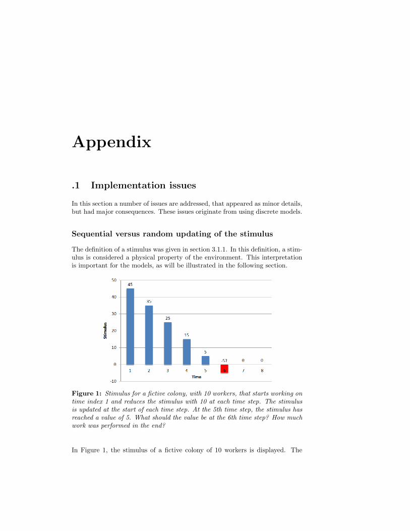
A threshold function is a function that takes the value 1 if a specified functionof the arguments exceeds a given threshold and 0 otherwise. Such a functionwas used for the first artificial neuron. This artificial neuron, was the ThresholdLogic Unit and was introduced in [38]. The input of a threshold function canbe interpreted as stimulus for a creature and the output as the binary response.The definition of a stimulus, as used in this paper, is:
A stimulus is a physical property of the environment, which is per-ceived and might trigger some behavioural response.
In this definition of a stimulus, it is not required that a worker reacts to thestimulus, merely the perception of the stimulus is enough. In the threshold mod-els a stochastic version of the threshold function is used and not the thresholdfunction as described above. In this stochastic version the probability that
14 Models on division of labour
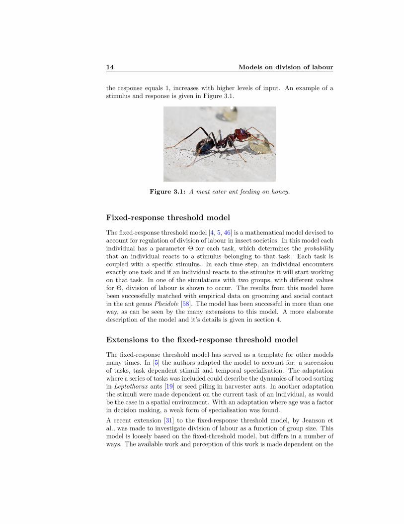
the response equals 1, increases with higher levels of input. An example of astimulus and response is given in Figure 3.1.
Figure 3.1: A meat eater ant feeding on honey.
Fixed-response threshold model
The fixed-response threshold model [4, 5, 46] is a mathematical model devised toaccount for regulation of division of labour in insect societies. In this model eachindividual has a parameter Θ for each task, which determines the probabilitythat an individual reacts to a stimulus belonging to that task. Each task iscoupled with a specific stimulus. In each time step, an individual encountersexactly one task and if an individual reacts to the stimulus it will start workingon that task. In one of the simulations with two groups, with different valuesfor Θ, division of labour is shown to occur. The results from this model havebeen successfully matched with empirical data on grooming and social contactin the ant genus Pheidole [58]. The model has been successful in more than oneway, as can be seen by the many extensions to this model. A more elaboratedescription of the model and it’s details is given in section 4.
Extensions to the fixed-response threshold model
The fixed-response threshold model has served as a template for other modelsmany times. In [5] the authors adapted the model to account for: a successionof tasks, task dependent stimuli and temporal specialisation. The adaptationwhere a series of tasks was included could describe the dynamics of brood sortingin Leptothorax ants [19] or seed piling in harvester ants. In another adaptationthe stimuli were made dependent on the current task of an individual, as wouldbe the case in a spatial environment. With an adaptation where age was a factorin decision making, a weak form of specialisation was found.
A recent extension [31] to the fixed-response threshold model, by Jeanson etal., was made to investigate division of labour as a function of group size. Thismodel is loosely based on the fixed-threshold model, but differs in a number ofways. The available work and perception of this work is made dependent on the
3.1 Models of division of labour in insects 15
colony size. Individuals encounter all tasks (instead of one at a time) and startworking on the first task, whose stimulus exceeds its thresholds. Individualsperceive the total stimulus divided by the number of workers, instead of thetotal. In this model division of labour was found to be increasing with colonysize.
Self-reinforcing response threshold models
From the fixed-response threshold models a number of self-reinforcement mod-els were derived. One of the first was [53], where the probability to performa specific task in the future is increased if a worker performs that task anddecreased if not working on that task. The parameter Θ of a task decreaseswhen working on that task, and is increased if not working on that task. Thismechanism leads to specialisation of individuals in tasks, since working on atask is a self-reinforcing act.
In a similar model [20], specialisation is an emergent property as a consequenceof colony size. This model has been extended again in [39] where the extensionsare: variable demands for work, an age-dependent parameter Θ and a finitelife span of the individuals. In this new model specialists occur as an emergentphenomenon dependent on the colony size.
3.1.2 Forage for work model
The forage for work model [55, 54] differs in several aspects from the ResponseModels. The first, is that workers are considered identical for this model, al-though this is not required. The second, is the explicit modelling of a spatialaspect of colony work. The main idea is that individuals work on a productionline (displayed in Figure 3.2), where work comes from the outside and is linearlyprocessed towards the center of the colony.
Figure 3.2: A production line of workers for three successive tasks. Individualscan move to a neighbouring patch or keep working on the current.
In each step, individuals will accept a task from their neighbour, process it, andgive the result to the other neighbour. Workers watch their neighbours, to seeif help is needed and move if required. In this way, each task will be done by
16 Models on division of labour
sufficient workers and the work load is evenly distributed among workers. Theseresults are robust; if a task needs change, the correct number of workers moveto regain the balance. The results of this model are in agreement with empiricalwork from [50]. The model received criticism (e.g. [56]), because of the lackof idle workers, the fact that all workers are identical and because only weaktemporal specialisation occurs.
3.2 Division of labour with (simulated) robots
3.2.1 The stick pulling experiment
A nice example of an experiment with division of labour, is the stick pullingexperiment [1, 30, 36]. In this experiment, workers have to work in pairs to beable lift sticks out of the floor, see Figure 3.3. The experiments were comparedto results from simulations and found to give qualitatively similar results. In [1]three threshold based allocation algorithms are compared in simulations, onebased on the fixed-threshold model, one where the thresholds are set by estima-tions of the agents, and one where agents could communicate global information.No difference in efficiency between these three mechanisms was found.
Figure 3.3: Arena with Khepera bots equipped with grippers. Because of thelength of the sticks, a single robot cannot pull a stick out of the ground.
3.2.2 Collecting food items with up to 12 mobile robots
A multi-robot system based on the fixed-response threshold model is given in[34], where up to 12 robots explored an area to find food. The robots inter-acted in the area mostly by staying out of each others way, which increased theefficiency in exploration. The efficiency of collecting food was measured for auniform distribution of food and for clustered food patches, while varying thegroup size. What they found for a uniform distribution was that a middle-sizedgroup had the best performance, because a small group repels other agentsenough to increase the efficiency of exploration, but not so much that robots
3.3 Summary of existing models 17
begin to hinder each other. For clustered food this effect was not significant.Information transfer between workers was implemented in a method similar totandem calling (tandem calling involves ants recruiting ants one at a time).When the food was clustered, tandem calling increased the efficiency of thecollection of food.
3.2.3 Strategies for energy optimisation
In [35] a simple adaptation mechanism to automatically adjust the ratio offoragers to resters in a swarm of foraging robots is introduced. Three adaptationrules were tested, internal rules (success of the robot itself), environmental cues(collisions with other robots) and social cues (success of other robots). What isfound is that social cues work best and have the most impact when food densityis low.
3.2.4 Transport through self-assembly
A recent paper where the way food is transported by individuals is evolved is[26]. Here it has been found that self-assembly can provide adaptive value forindividuals that compete in an artificial evolution based on task performance.This shows how group transport could have evolved from solitary transport.
3.2.5 Complex foraging with multiple sub goals
How up to 12 mobile robots solve a complex foraging task is described in [42].The task requires group coordination at several stages. Food is localised byforming a chain from the nest to a food item. After a chain is formed and enoughrobots have been gathered at the food location, the food is collectively broughtback to the nest. Because the food item is too heavy for an individual robot,the robots have to cooperate. The robots used for this experiment are identicalswarm-bots, with identical control mechanisms. The control mechanism is ahand crafted finite state machine, where some underlying behaviours have neuralnetwork controllers, with weights that are evolved by a genetic algorithm.
3.3 Summary of existing models
The current models on insects show designed mechanisms that lead to speciali-sation through self-organisation, which gives insight about how individual andcolony-level behaviour could be related. The self-organisational models thathave been found, are often robust to internal and environmental changes e.g.[55, 54]. None of these models can explain how division of labour could haveevolved, which is the main critique of the author on these models.
18 Models on division of labour
The research with robots shows great promise for finding mechanisms for di-vision of labour, but a problem with real robots is that it usually is too time-consuming to use evolutionary approaches. Modelling division of labour insimulations allow an evolutionary approach, but care should be taken to avoidoversimplifying the environment and or workers. In summary, the existing mod-els could greatly benefit from using an evolutionary perspective and from theinsights gained from robots and simulations thereof.
Chapter 4
Fixed-response thresholdmodel
4.1 Introduction
The fixed-response threshold model [4, 46] is the most popular model on divisionof labour in insect societies. This model simulates the dividing of work ofa colony within one generation. Because the model serves as a basis for thefollowing models, the dynamics of this model are explored first. By rebuildingan existing model, the properties of the model can be investigated and comparedto the other models in this thesis.
4.2 Methods
Each individuals has a parameter Θ for each task, which determines the proba-bility that an individual reacts to a stimulus belonging to that task. A stimulustriggers exactly one behaviour and the probability of reacting increases with theintensity of the stimulus. If a stimulus is not strong enough to trigger an action,a worker does nothing. The probability that an individual i, with parameter Θ,reacts to a stimulus s is given by:
T (s) = Pi(X = 0→ X = 1) =s2
s2 + Θ2i
(4.1)
Where X is the state of an individual (X = 0 equals inactivity and X = 1is equal to performing a task), and Θi is the parameter that influences thesensitivity of a worker i to a stimulus (s). This function is a sigmoid, where theparameter Θ displaces the graph horizontally, as can be seen in Figure 4.1.
Individuals encounter one of two tasks at random with probability 0.5. In each
20 Fixed-response threshold model
Figure 4.1: The probability T that an individual starts working on a task, as afunction of the stimulus s for that task, for different values of Θ. The probabilityof reacting to a stimulus level decreases with higher values of Θ.
time step an individual can work on that task, or do nothing. Once working, theindividual will continue to perform a task, until it quits with a fixed probabilityp. Note that the quitting probability is independent of the stimulus level. Afteran individual stops working on a task, it can only start working again in the nexttime step. Stimuli increase with a fixed amount δ per time step. Working ona task, decreases the stimulus of that task with a fixed amount per individual.The environment is only affected by the colony and not by outside influences(closed world assumption). There are two tasks and two groups of individuals(castes), which differ in their value of Θ. The settings for the simulations aregiven below.
Parameter Value Parameter Valueindividuals (N) 100000 Θtask0 group 0 1work per individual 1/N Θtask1 group 0 8individuals group 0 50000 Θtask0 group 1 8individuals group 1 50000 Θtask1 group 1 1stimulus increase (δ) 0.1 probability to quit (p) 1time steps 140 tasks 2
Table 4.1: Parameter settings for the simulations. Note that the increase of thestimulus is defined in terms of the maximum amount of work that a colony cando at each time step. The stimulus increase is less than the maximum of whata colony can do, otherwise stimulus levels continue to increase. The probabilityto quit is equal to 1, since this results in individuals choosing their actions ateach time step. This set of parameters is chosen, because with different groupsdivision of labour is expected to occur.
4.3 Results 21
4.3 Results
The results with a quitting probability of 1 are shown in Figure 4.2.
(a) Percentage of active workers of 2 castes, where each caste prefers a differ-ent task. An equilibrium is reached after approximately 50 time steps, when10% of the colony works on each task, matching the stimulus increase.
(b) Stimulus levels of the 2 tasks. Stimulus levels increase, until the increaseis matched with the work of the colony.
Figure 4.2: Percentage of workers and stimuli for 2 groups and 2 tasks, withp = 1. In equilibrium workers divide the 2 tasks among the 2 castes.
It is clear from Figure 4.2(a) that each caste works predominantly on their pre-ferred task. The non-preferred task has a low probability of being performed,but is not equal to zero. The active workers of each caste reach an equilibriumquite soon. For the preferred tasks the equilibrium is near 10% of the total num-ber of workers. This percentage is no surprise, since the increase of the stimulus
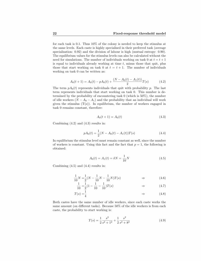
22 Fixed-response threshold model
for each task is 0.1. Thus 10% of the colony is needed to keep the stimulus atthe same levels. Each caste is highly specialised in their preferred task (averagespecialisation: 0.92) and the division of labour is high (mutual entropy: 0.90).The equilibrium values for the stimulus levels can also be calculated without theneed for simulations. The number of individuals working on task 0 at t = t+ 1is equal to individuals already working at time t, minus those that quit, plusthose that start working on task 0 at t = t + 1. The number of individualsworking on task 0 can be written as:
A0(t+ 1) = A0(t)− pA0(t) +(N −A0(t)−A1(t))
2T (s) (4.2)
The term pA0(t) represents individuals that quit with probability p. The lastterm represents individuals that start working on task 0. This number is de-termined by the probability of encountering task 0 (which is 50%), the numberof idle workers (N −A0 −A1) and the probability that an individual will workgiven the stimulus (T(s)). In equilibrium, the number of workers engaged intask 0 remains constant, therefore:
A0(t+ 1) = A0(t) (4.3)
Combining (4.2) and (4.3) results in:
pA0(t) =1
2(N −A0(t)−A1(t))T (s) (4.4)
In equilibrium the stimulus level must remain constant as well, since the numberof workers is constant. Using this fact and the fact that p = 1, the following isobtained:
A0(t) = A1(t) = δN =1
10N (4.5)
Combining (4.5) and (4.4) results in:
1
10N =
1
2(N − 1
10N − 1
10N)T (s) ⇒ (4.6)
1
10=
1
2(1− 1
10− 1
10)T (s) ⇒ (4.7)
T (s) =1
4⇒ (4.8)
Both castes have the same number of idle workers, since each caste works thesame amount (on different tasks). Because 50% of the idle workers is from eachcaste, the probability to start working is:
T (s) =1
2
s2
s2 + 12+
1
2
s2
s2 + 82(4.9)
4.3 Results 23
The last equation is obtained by combining (4.8) and (4.9):
T (s) =1
2
s2
s2 + 12+
1
2
s2
s2 + 82=
1
4⇒ s ≈ 0.98 (4.10)
This matches the results obtained from the simulations (see Figure 4.2(b)).
In the next simulation, parameter p is changed to 0.2, which changes the dy-namics slightly, see Figure 4.3.
(a) Percentage of active workers of two castes for 2 tasks. Around t = 15there is an overshoot of workers, which quickly decreases in amplitude.
(b) Stimulus levels of two castes (roles) for two tasks. The Oscillations dueto the delay in the system can be clearly seen.
Figure 4.3: Percentage of active workers and stimuli for two castes, withp = 0.2. Work is divided between the castes. The quitting probability causes adelay in the response and results in an overshoot of assigned workers.
24 Fixed-response threshold model
By changing the parameter p to 0.2, the system shows a delay. This delay can beclearly seen in graphs 4.3(a) and 4.3(b). It can be seen that the stimulus peaksfirst and after a short delay the workers (over)react. The delay is caused by thefact that individuals continue working independent of the stimulus levels. Theequilibrium for the active workers is not changed by the quitting probability,but the equilibrium for the stimulus levels is. The equilibrium can be derivedanalogous to the previous simulation. This is because workers perform a task fora period of 5 time steps on average, independent of the stimulus levels. Thus,much lower stimulus levels are needed to get the required number of workers.
4.4 Discussion
What can be seen in this model is that division of labour is quite high (mutualentropy = 0.90). There are two groups (castes) within a colony, with fixedvalues for Θ, working on two different tasks. The colony reaches an equilibriumafter about 30 time steps, when the actions of the colony match the increase ofthe stimuli. The quitting probability affects the response time in the colony, itcan be seen as a delay in the system response. These results match the resultsas found in [4].
Although this model shows division of labour, the results are not surprising. Bycreating two groups, each with a preferred task, division of labour is built intothe model. Furthermore, p < 1 guarantees some level of specialisation, sinceindividuals are forced to stick with their tasks. This model does show that withthese settings division of labour is possible and this provides a starting point forfurther investigations. These results do not show how division of labour couldhave evolved, or how division of labour could be an emergent property. Toconclude, this model shows division of labour can be obtained with a designedmechanism, but cannot explain division of labour as an emergent property.
Chapter 5
Evolutionary fixed-responsethreshold model
5.1 Introduction
In the previous section, the fixed-response threshold model [4] was explored.High levels of division of labour were obtained in the simulations, but only as aconsequence of designed mechanisms. This provides a starting point for furtherinvestigations, but leaves many questions unanswered. In this model, division oflabour is studied as an emergent property. By studying division of labour as anemergent property, it is possible to study the conditions, that lead to division oflabour. The focus of this chapter is the evolution of division of labour. Divisionof labour is not directly rewarded and there is no designed mechanism thatensures division of labour. The main idea of the model is that evolutionarypressure could exist to work on multiple tasks in a specific ratio. An examplecould be an ant colony that needs to forage for two kinds of food in a ratiothat is optimal for their nutritional needs. The question for this model is: Doesevolutionary pressure for performing tasks in a specified ratio lead to divisionof labour?
5.2 Methods
Within one generation, this model is identical to the fixed-response thresholdmodel of the previous section 1. Individuals encounter one task at a time and candecide whether they react to the stimulus and start working on the task. Stimuliincrease with a fixed amount δ per time step. The difference with the previousmodel is that the preference of individuals to work on a task is hereditary. The
1For details of the fixed-response threshold model, see section 4.2
26 Evolutionary fixed-response threshold model
probability that an individual i, with parameter Θ, reacts to a stimulus s is thesame as in the previous model and is defined as:
T (s) = Pi(X = 0→ X = 1) =s2
s2 + Θ2i
In this model the parameter Θ is hereditary. By inheriting this parameter anindividual has inherited a preference for working on tasks. A general overviewof the model is given below. Each of these steps is explained in detail in thefollowing sections.
0) 2N haploid individuals (parents) are initialised
For each generation:
1) N colonies are formed from 2N haploid parents
2) Colony is simulated during one season:
For each colony:
For each time step:
For each worker in colony:
2.1) Worker chooses behaviour based on stimuli
2.2) If possible worker performs chosen behaviour
2.3) Stimulus is updated
3) Fitness of each colony is calculated
4) 2N new parents are selected based on colony fitness
5) Back to step 1 until end of simulation
Step 0: Initialise 2N haploid parents
In the first generation of the simulation 2N parents are initialised, each witha set of genes. Parents are haploid and have exactly one gene for each task.Note that in nature workers are diploid (two of each gene), but for simplicitythis model assumes haploidy. Genes encode parameter (Θ). The genes areinitialised by randomly drawing a value from a uniform distribution between 0and 10. Although a uniform distribution is used to create initial variation inthe genes, any distribution that introduces variation suffices.
Step 1: Create N colonies from 2N haploid parents
At the start of a generation two parents from the previous generation form a newcolony. A colony has a fixed number of haploid workers, that are formed by fullrecombination of the parents. This means that workers have a probability of 0.5per gene to inherit the gene from either parent. In addition to recombination,each gene has a probability to mutate. The size of the mutation is drawn froma normal distribution.
5.2 Methods 27
Step 2: Colony is simulated during one season
During a simulation a colony is simulated for one season. This means that eachcolony is simulated for a fixed number of time steps. At each time step, all theindividuals of a colony get a chance to work. The order at which individualswork is randomised. Working can be divided into three parts:
Step 2.1: Worker chooses behaviour
Each non-active worker encounters a random task, with an equal probability foreach task. When a worker encounters a task it can either work on that task ordo nothing this round. The probability that a worker will react to a stimulus isdetermined by equation 5.2. Once an individual is working on a task it has afixed probability p to quit, and will not re-evaluate stimulus levels during work.
Step 2.2: Worker performs chosen behaviour
After a worker has chosen a behaviour, it will try to perform the chosen be-haviour, and normally this is allowed. Only if the act of working on the chosenbehaviour would lead to a negative stimulus level, the work is not allowed. Ifthe chosen behaviour is not allowed, the worker must skip this turn.
Step 2.3: Stimulus is updated
The stimulus is updated after each worker has performed an action. By updatingafter each action, each worker perceives current value of the stimulus. Thereforethe stimulus is not the same for each ant. This way of updating does make theorder of the workers a factor. The last selected member of a colony perceives amuch lower stimulus than the first. To prevent the order of working influencingthe results, the order is randomised.
Step 4: Calculating fitness
A fitness function is crucial in an evolutionary simulation, since it (indirectly)determines what will evolve. For this model colony-level selection was chosen, sothat colonies receive a fitness value, but not the individuals within a colony. Thefitness of a colony is based on it’s worker distributions. To obtain a high fitness,a colony should assign worker to the tasks in a proportion that is specified inthe fitness function. In this model, the fitness function described in [15] waschosen, in which the fitness of a colony c is defined as:
F (c) =
m∏t=0
pγtt where∑t
γt = 1 (5.1)
28 Evolutionary fixed-response threshold model
Where pt is the proportion of work done for task t, relative to the capacity ofthe colony. The number of tasks is m and γt is an exponent that determines theoptimal worker distribution. This function has the property that it maximizeswhen a colony has the worker distribution that equals γt for each task t. Forexample if there are two tasks with γ1 = 0.2 and γ2 = 0.8, then the maximumof the fitness function is when a colony has worked on task 1 with 20% of it’sworkers and 80% on task 2.
Step 5: Create 2N haploid parents from selected colonies
Relative fitness-proportional selection is used to select the colonies that mayreproduce. The probability that a colony c from K colonies may reproduce is:
pc =fc − fminΣKc=1fc
(5.2)
Where fc is the fitness of colony c and fmin is the fitness of the colony with thelowest fitness. This means that the colony, with the lowest fitness, cannot haveoffspring. For the other colonies the probability to have offspring increases withtheir fitness. If a colony is selected, a random worker from the colony is selectedto be a parent for a new colony.
Step 6: End of a generation
If the number of generations does not exceed the total number of generationsspecified for the simulation, the cycle is repeated from step 2. If the maximumspecified number of generations is reached, the simulation is ended.
Settings
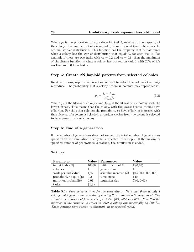
Parameter Value Parameter Valueindividuals (N) 10000 initial distr. of Θ U(0,10)colonies 1 generations 1work per individual 1/N stimulus increase (δ) {0.2, 0.4, 0.6, 0.8}probability to quit (p) 0.2 time steps 140mutation probability 0.01 mutation size N(0, 0.01)tasks {1,2}
Table 5.1: Parameter settings for the simulations. Note that there is only 1colony and 1 generation, essentially making this a non-evolutionary model. Thestimulus is increased at four levels of δ, 20%, 40%, 60% and 80%. Note that theincrease of the stimulus is scaled to what a colony can maximally do (100%).These settings were chosen to illustrate an unexpected result.
5.3 Results 29
5.3 Results
The first result (Figure 5.3) shows the resulting fitness for different values ofΘ for one task. There are four different simulations, which differ only in therate of increase (δ) of a task. The perhaps surprising result is that the fitnessis completely independent of the preference of individuals (i.e. parameter Θ).
Figure 5.1: Different simulations for four levels of growth of the stimulus (20%,40%, 60% and 80%) as a function of the threshold (Θ). The fitness levels aredependent on the stimulus increase, but not on parameter Θ.
5.3.1 Damped stimulus growth
A different function for the stimulus increase was chosen so that (Θ) has an effecton the fitness. Contrary to the previous simulation the stimulus is not increasedby a fixed amount per round, but the increase of the stimulus is dependent onthe stimulus itself. This stimulus increase is defined as:
s(t) = s(t− 1) + gmax ∗(smax − s(t− 1))
smax(5.3)
Where smax is the maximum value of the stimulus and gmax is the maximumgrowth of the stimulus. This results in an initial rapid stimulus increase, butdeclines as the total stimulus level increases. When the stimulus level reachesthe maximum value, the growth is zero.
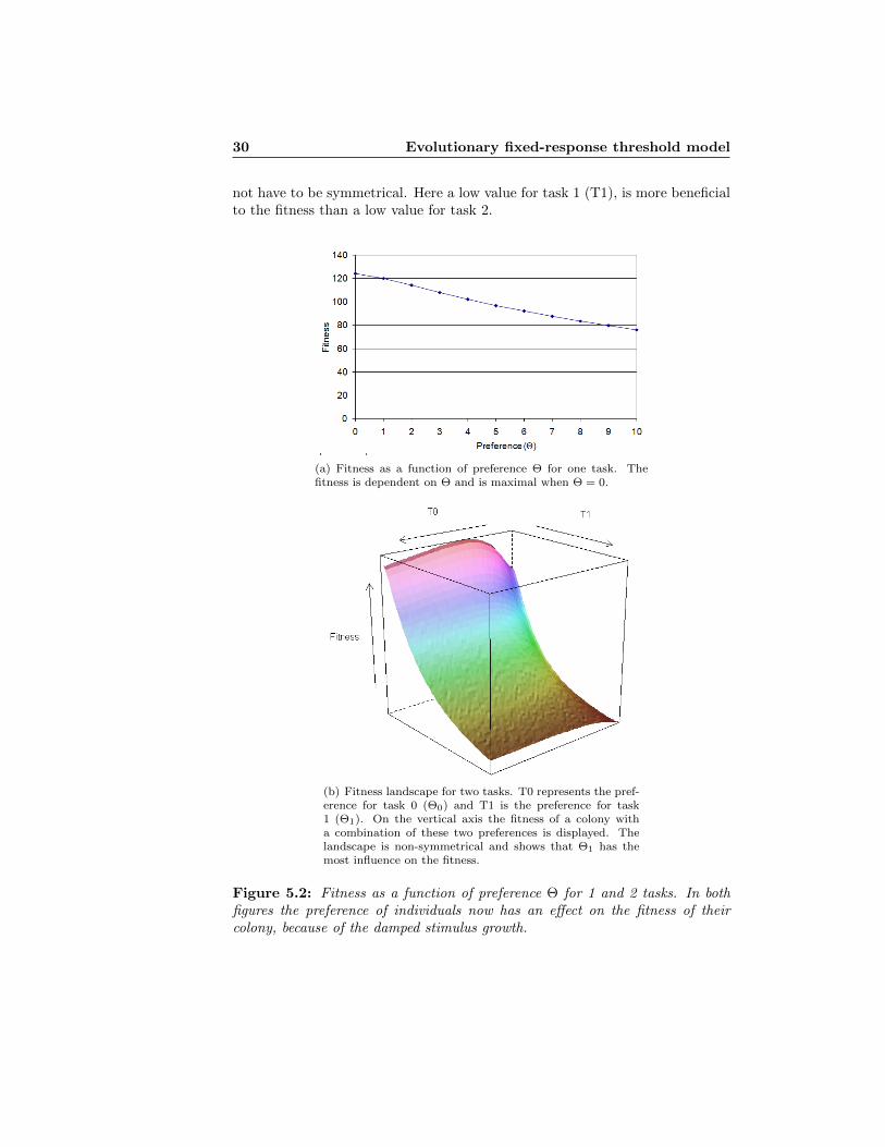
The effect of this function on the fitness landscape can be seen in Figures 5.2(a),5.2(b) for 1 and 2 tasks respectively. In both figures the fitness clearly dependson the thresholds. From Figure 5.2(b) it is clear that the fitness landscape does
30 Evolutionary fixed-response threshold model
not have to be symmetrical. Here a low value for task 1 (T1), is more beneficialto the fitness than a low value for task 2.
(a) Fitness as a function of preference Θ for one task. Thefitness is dependent on Θ and is maximal when Θ = 0.
(b) Fitness landscape for two tasks. T0 represents the pref-erence for task 0 (Θ0) and T1 is the preference for task1 (Θ1). On the vertical axis the fitness of a colony witha combination of these two preferences is displayed. Thelandscape is non-symmetrical and shows that Θ1 has themost influence on the fitness.
Figure 5.2: Fitness as a function of preference Θ for 1 and 2 tasks. In bothfigures the preference of individuals now has an effect on the fitness of theircolony, because of the damped stimulus growth.
5.4 Discussion 31
5.4 Discussion
The results show a surprising property of the evolutionary fixed-response thresh-old model. The fitness is clearly independent of the preference of individuals (i.e.parameter Θ). Parameter Θ does not have any effect on the number of workersassigned to each task. This is because at equilibrium the colony will work asmuch per time step as the increase of the stimulus. This can be explained bythe following rationale.
If a colony would work less than the amount at which a stimulusincreases at each time step, then the level of the stimulus increases.The increase of the stimulus causes more workers to be assignedto the associated task, since higher values of the stimulus increasesthe chance that insects start working on the task. As long as thestimulus increase is not larger than the total number of workers ina colony, an equilibrium is eventually reached and the colony worksat exactly the same pace as the increase of the task.
On the other hand, if a colony would do more work than the amountat which a stimulus for some task increases at each time step, thestimulus level for that task is reduced. Reduction of the stimulusresults in less workers for the task. Until eventually an equilibriumis reached, where the number of workers is equal to the stimulusincrease.
It can be seen that the preferences do not matter at all. Whatever the prefer-ences of a colony, in the end the stimulus will get high enough (or low enough)so that a colony will perform exactly the same amount of work as the increase ofwork. Colonies are completely inflexible in choosing their work ratios in reactionto stimuli. This is a surprising, but important result, that gives new insightsabout the dynamics in these types of models. It is an important result, sincemany of the current models have dynamics very similar to the model discussedin this chapter.
The results from using a damped stimulus increase show that a colony can haveinfluence on its fitness (by changing their preferences). The colony can havean influence on the fitness because the total stimulus level affects the stimulusincrease. If a colony can keep stimulus levels low, then the increase is maximaland more work can be done. However the mechanics in this simulation are quiteinflexible and largely determined by the growth rate of the stimulus. In essence,the colony is almost as inflexible as it was. Furthermore, the stimulus dynamicsnow model only a small subset of the stimuli, as can be expected in the realworld. Clearly, changing the stimulus dynamics in this way cannot be used asa general model for division of labour in insects.
In conclusion, unexpectedly the preference of individuals does not have anyinfluence in this model, which places many existing models on division of labour,with the same kind of dynamics in a new light.
32 Evolutionary fixed-response threshold model
Chapter 6
Evolutionary non-spatialneural network model
6.1 Introduction
In the evolutionary fixed-response threshold model, the results showed that acolony was unable to choose work ratios given the stimulus increase of tasks.Because of this, specialisation and division of labour could not evolve in themodel. In this model a new and more open behaviour mechanism is chosen.The model in this section is an adaptation of the previous model, where thebehaviour mechanism is changed to a feed-forward neural network (A neuralnetwork, where information flows in one direction only). The neural network iskept simple (i.e. no learning and no recurrent connections), to make it possibleto understand these dynamics in full, within the time frame of this thesis. Themodel is meant as a stepping stone for more complicated models, and is designedfor future expansions (such as including learning, modelling spatial settings,and the implementation of more complex interactions). The main questionfor this evolutionary neural network model is: Does rewarding specific workerdistributions lead to division of labour?
6.2 Methods
The simulation is based on the evolutionary fixed-response threshold model ofthe previous chapter. The first stimulus update function of the previous chapteris used, where the stimulus is updated with a fixed amount (δ) per time step.This model is exactly the same model as the one discussed in the previous
34 Evolutionary non-spatial neural network model
section, with the exception of two changes1:
1. After quitting a task, workers no longer have to skip a turn.
2. The behaviour mechanism is replaced by a feed-forward neural network.
The first change is a minor one. The probability to quit remains, but afterquitting to work on a task, a worker can immediately begin on a new one. Atthe start of a time step, a worker has to decide if it wants to continue workingon the current task. In this way, workers can never perform more than one taskin each time step. This change is more a simplification, than a change, since thismakes workers act in a similar way each round. This makes the model easierto understand and does not give qualitatively different results. This is a minorchange of the model, but the model has a more significant change, which is anew behaviour mechanism.
6.2.1 Feed-forward neural network
This model uses a simple kind of artificial neural network, where informationis passed in one direction only, from stimuli, via hidden neurons, to behaviourneurons. These types of artificial neural networks are also called linear thresholdunits or perceptrons and are described in [38, 41, 47]. Artificial neural networksare based on biological neurons such as those described in ants in [21]. Anillustration of a possible network structure is given in Figure 6.1.
The network from the illustration consists of three layers. Each layer is fullyconnected to the next layer and each of these connections has a weight associatedwith it. The first layer is the input layer, where the inputs are stimuli that arepotentially associated with tasks. The number of inputs to the first layer is equalto the number of stimuli. The inputs are connected to the next layer, each ofthese connections has a weight wij associated with it. The next layer is a hiddenlayer and consists of a series of neurons, each of which receives inputs from itsincoming connections. Each neuron sums up all of the inputs it receives. Theseinputs are stimuli multiplied by the weights of the connections and a bias. Thefollowing equations for the feed-forward network are obtained from standardliterature on neural networks [27, 48]. The neurons calculate their activationsaccording to the following equation:
a = bi +
n∑i
xiwij (6.1)
The activation a of a neuron is the sum of all the inputs to that neuron. Theinputs are products of the weights multiplied by the outputs of the previouslayer(stimulus), plus the bias. The bias bi can be different for each neuron
1Actually a third change is that this model has been written using an object orientedprogramming style for maintainability and understandability[6].
6.2 Methods 35
Figure 6.1: Feed-forward network with 2 inputs (stimuli), 1 hidden layer (with2 neurons), and 3 output neurons (behaviours). Each neuron receives inputsfrom the previous layer and one input from the bias. A bias is a clamped valuethat is independent of the input. Note that the input layer does not consist ofneurons, only of inputs, and is therefore not connected to the bias.
due to the connection weights. The output of neurons from the hidden layeris calculated by applying the sigmoid function to these activation values. Theoutput of a neuron is defined as:
P (a) =1
1 + e−a(6.2)
Note that the output is always positive, even though the weights, bias andactivation can be negative. These outputs are multiplied by weights (wjk) andare inputs for the next layer. These neurons calculate their outputs accordingto equations (6.1) and (6.2). The number of inputs and outputs varies with thenumber of tasks. The number of hidden layers can be zero or higher, without ahidden layer the inputs are fully connected to the outputs. Note that the inputlayer does not consist of neurons unlike the hidden and output layers.
For this model, the choice was made that output levels determine the probabil-ities of the behaviours. The relative output level of a neuron, compared to theother neurons, determines the probability of firing. This method was selected,since it resembles the mechanism of the fixed-threshold model, which makes iteasier to compare the different models. With this implementation the stimulusintensity determines the probability of an individual to engage in that task, aswas the case in the response model.
36 Evolutionary non-spatial neural network model
Inheritance
Genes encode the weights of the neural network and the bias. When genes areinherited from the parents, there is a probability of 0.01 of a mutation per gene.If a gene is mutated, the size of the mutation is drawn from a normal distributionN(0, 0.01). Two modes of inheritance are tested: full (uniform) recombinationand linked genes. With full recombination, each gene has a probability of 0.5 tobe inherited from either parent. With linked genes each worker gets all genesfrom one parent, with a probability of 0.5 for either parent. In this case, allgenes are inherited as one package. Inheriting all genes from one parent resultsin offspring that is very similar to the parents. If a colony is successful, itis likely that the offspring is successful too. When colonies reproduce with fullrecombination, the offspring is likely to be very different from the parent colony.Depending on the variation within a population, full recombination can be verydisruptive [12].
Replicates
The simulations were performed with 5 replicates. Each replicate is an evo-lutionary run of a population of colonies. Each replicate is executed with adifferent seed, but otherwise with the same simulation parameters. For practi-cal purposes replicates can be viewed as being completely independent simula-tions, although the simulations use the same random number generator (Witha different seed.).
6.2.2 Settings
Parameter Value Parameter Valuetime steps 100 mutation probability 0.01incr. food 1 100% mutation size N(0, 0.01)incr. food 2 101% tasks 3colonies 1000 goal ratio of tasks {0,1,2} {0, 7
10 ,310}
generations 1000 prob. to quit 1hidden layers 0 workers per colony 100
Table 6.1: Parameter settings for the simulations. The increase of the stimulusper time step is defined in terms of the work capacity of a colony. With thesesettings stimulus values keep increasing and are never depleted. The probabilityto quit at each time step is set to 1, which makes individuals select a behaviour ateach time step. Lower values do not result in qualitatively different results, butdo affect the measure of division of labour. This is because lower probabilitiesforce individuals to stick to tasks and this is exactly what is measured for divisionof labour.
6.3 Results 37
There are 3 tasks, the first of these does not contribute to the fitness and hasno associated fitness. This first task represents a task as moving between tasks,which usually does not directly contribute to the fitness. The fitness functionwith these parameters is:
F = p00 × p7101 × p
3102 (6.3)
Where p0,1,2 represent the proportion of work on tasks {0,1,2}, relative to thecolony capacity. The optimal worker ratios can be calculated by realising thatno effort should be spend on task zero, since it does not count for the fitnessfunction. Thus all the work should be divided over task 1 and task 2. Now 6.3can be rewritten to:
F = p00 × p7101 × p
3102 = 1× p
7101 × (1− p1)
310
This is maximal when the derivative is equal to zero, thus:
0 =dF
p1(p
7101 × (1− p1)
310 ) ⇒
0 =7
10p
−3101 (1− p1)
310−3
10p
7101 (1− p1)
−710 ⇒
0 = 1−310p
7101 (1− p1)
−710
710p
−3101 (1− p1)
310
⇒
0 = 1− 3
7p1(1− p1)−1 ⇒
p1 =7
10⇒ p2 =
3
10(6.4)
6.3 Results
In the first section, the ability to evolve worker ratios, that result in high fitnesslevels, is investigated.
6.3.1 Worker ratios
With recombination the results for the evolution of worker ratios are displayedin Figure 6.2(a). It can be seen that for each task the optimal ratio, as definedby the fitness function, is found. The optimal ratios are found within 300generations and soon there is no variation left.
With linked genes the optimal proportions are also found, although at a slightlyslower pace (Figure 6.2(b)) The results are quite similar to Figure (a), in bothcases the optimal ratios are found quite fast.
38 Evolutionary non-spatial neural network model
(a) Average task ratios for three tasks of colonies, with recombination. Afterapproximately 300 generations the optimal proportions are found.
(b) Average task proportion of three tasks of colonies, with linked genes.After approximately 300 generations the optimal proportions are found.
Figure 6.2: Average worker ratios. Tasks are represented by color, task 1 isprinted in blue (top), task 2 in green (middle) and task 0 in red (bottom). Errorbars show one standard deviation, visible as a cloud. Optimal task proportionsfor all three tasks are quickly found with recombination and with linked genes.
6.3 Results 39
6.3.2 Division of labour
The measure used for division of labour is mutual entropy (see section 2.3). Inessence, the measure captures individual and task specialisation and is thereforewell-suited as a measure for division of labour. In Figure 6.3 the average levelsof division of labour are shown for five populations.
(a) Average division of labour of colonies with recombination. One replicatehas relatively higher values for division of labour(0.3), compared to the otherreplicates.
(b) Average division of labour of colonies with linked genes.
Figure 6.3: Average division of labour of five replicates with 1000 colonies.Error bars show one standard deviation, visible as a cloud. Levels of division oflabour decline, but variation remains high, since division of labour is indirectlyevolved and does not appear to influence fitness much at these levels.
40 Evolutionary non-spatial neural network model
With both modes of inheritance, the level of division of labour that is evolvedis low. Interestingly, one population of colonies evolves toward a significantlyhigher rate of division of labour compared to the other populations, althoughthe level of division of labour that is reached (0.3) is low in the absolute sense.This population did have recombination, but other simulations show this alsohappens with linked genes. Varying levels of division of labour can be evolved,because division of labour has no direct influence on the fitness of colonies. Allof the populations reach near optimal fitness levels, even though division oflabour levels are low.
The evolved level of division of labour shows what type of strategies are easiestto evolve. With these forward neural networks and a stochastic method to selecttasks, the easiest solution is to let workers switch often. Switching between tasksis easier, since it allows all workers to be genetically similar and this makes themless susceptible to disruptive recombination.
6.3.3 Adding a switching cost
Workers from insect colonies usually have some cost associated with switchingbetween tasks. For example, in any spatial environment, switching betweentwo separate locations takes some time. Another possible switching cost is themental cost for switching between tasks, since switching might require memoryand a cognitive architecture that can perform two different task shortly aftereach other. In this model, a switching cost is implemented as a time penaltyfor switching between tasks. Although the model is non-spatial, this choicefor a switching cost is a first step towards a spatial model. During a timepenalty workers cannot perform any action. Because the fitness function rewardsthe proportion of workers that work, this time penalty decreases the fitness ofcolonies that switch often.
Division of labour with a switching cost
When introducing a switching cost of 1 the level of division of labour thatis evolved is quite different. Both with recombination and with linked genesdivision of labour is evolved to quite high values (Figures 6.4(a), 6.4(b)).
There are some differences between the two graphs, the division of labour at-tained with linked genes is slightly higher, and has a much higher standarderror. Increasing the switching cost to 3, 5, 7 or 9 does not change the resultssignificantly.
6.3 Results 41
(a) Average division of labour of colonies with recombination.
(b) Average division of labour of colonies with linked genes.
Figure 6.4: Average division of labour of colonies, with switching cost = 1.Error bars show one standard deviation, visible as a cloud. With linked genes theaverage division of labour reaches a higher value (0.8) than with recombination(0.75), although the standard deviation with linked genes is much higher. Inboth graphs division of labour is clearly favoured when a switching cost is added.
Worker ratio flexibility with a switching cost
When looking again at the worker ratio flexibility, but now with a switchingcost, a new pattern emerges. Average proportions of work, with recombinationand with linked genes, are displayed in Figures 6.5(a) and 6.5(b).
42 Evolutionary non-spatial neural network model
(a) Average task proportions for three tasks, with recombination. Near op-timal values are found within 200 generations.
(b) Average task proportions for three tasks, with linked genes. The ratioof task 0 reaches near optimal value of 0, but task 1 and task 2 have clearlysuboptimal proportions. The ratio of task 1 is about 0.5, while task 2 iscloser to 0.4.
Figure 6.5: Average task ratios with switching cost = 1. Tasks are repre-sented by color, task 1 in blue (top), task 2 in green (middle) and task 0 inred (bottom). Error bars show one standard deviation, visible as a cloud. Withrecombination near optimal values are found, while with linked genes ratios areclearly suboptimal.
Recombination leads to optimal ratios, but with linked genes these ratios arenot reached. This pattern repeats itself when the switching cost is increased to3, 5, 7 and 9. With linked genes (no recombination) the correct worker ratioscannot be evolved. With linked genes all the genes of workers are inherited from
6.3 Results 43
either parent. If one parent prefers to work on one task and the other parenton another, this leads to the situation where 50% of the workers prefers thefirst task and 50% preferring the other task. The 50/50 ratio is a consequenceof the fact that each worker has a probability of 0.5 to inherite all genes fromeither parent. Thus if both parents prefer a different task, the colony will notbe able to work with the optimal ratios. An even worse problem exists whenboth parents prefer the same task. In that situation the entire colony will preferto work on one task, which leads to specialisation, but not division of labour. Ifa colony works only on one task, the colony is severely puninshed with a fitnessof 0. These two problems illustrate the limitations of full linkage of the genes.
Fitness levels with a switching cost
The fitness measure, that is used here is a normalised version of the fitnessfunction (F(c)) in the previous chapter (equation 5.1). This normalised fitnessfunction is:
Fn(c) =F (c)
Max(F (c))where F (c) =
m∏t=0
pγtt and∑t
γt = 1 (6.5)
From Figure 6.6 it can be seen that the failure to evolve the specified workerratios with linked genes is reflected in the fitness of the colonies. This can beexpected since the fitness function specifically rewards worker ratios. With re-combination (fig 6.6(a)) the fitness levels that are reached are significantly higherthan with linked genes (fig 6.6(b)) with (p < 0.01 for generation 1000 using theWilcoxon signed rank test). The difference in fitness between recombinationand linked genes increases with higher switching costs.
44 Evolutionary non-spatial neural network model
(a) Average fitness values for colonies with recombination. An equilibriumfor a fitness value of 0.9 is reached within 100 generations.
(b) Average fitness values for colonies with linked genes. An equilibrium fora fitness value of 0.8 is reached within a 100 generations
Figure 6.6: Average normalised fitness (switching cost = 1). Error bars show1 standard deviation, visible as a cloud. The average fitness with recombinationis higher and has significantly less variation.
6.3 Results 45
Fitness levels within a colony
A problem for colonies with linked genes is when two parents both prefer thesame task. Throughout the simulations the colonies with linked genes sufferfrom combinations of too similar parents and fitness levels of low levels continueto exist in the population (see fig. 6.7).
(a) With recombination all evolved colonies quickly reach high fit-ness values
(b) With linked genes a significant portion of the population suffersfrom a bad combination of two similar parents, resulting in lowfitness values.
Figure 6.7: Individual fitness levels and average (red line) of a population ofa 1000 colonies for switching cost = 5. This switching cost was selected, sinceit shows the horizontal bands most clearly, but the effect is visible as well withother switching costs.
46 Evolutionary non-spatial neural network model
Individual colony behaviour
With recombination and a switching cost, division of labour and optimal workratios can be evolved, but what is the behaviour of individuals?
Without a switching cost the evolved strategy is to let each ant have a prob-ability of 0.7 to work on task 1 and 0.3 to work on task 2. Thus without aswitching cost behaviour is not really interesting, but with a cost to switchingdifferent strategies are required. Displayed below are the individual colony workratios over time. With a switching cost and with recombination the colonies stillmanage work ratios, close to the optimum, with slight oscillations (see Figure6.8).
Figure 6.8: Actions of one colony, with switching cost = 1, with recombination.Top (orange) line is the sum of all actions, green (second from top) = task 1,blue = task 2, red (bottom) is task 0, dashed line = ’waiting due to switching’.Behaviours oscillate around optimal ratios.
With linked genes the strategies are similar but now with completely straightlines (see fig. 6.9(a)). Furthermore oscillations are generally stronger in colonieswith linked genes (see fig. 6.9(b)).
6.3 Results 47
(a) Actions of one colony with linked genes. After the initial phasework ratios are completely constant.
(b) Actions of one colony with linked genes. Heavy oscillations canbe seen between task 1 and task 2
Figure 6.9: Actions of one colony, with switching cost = 1, with recombination.Top (orange) line is the sum of all actions, green (second from top) = task 1,blue = task 2, red (bottom) is task 0, dashed line = ’waiting due to switching’.
48 Evolutionary non-spatial neural network model
6.4 Discussion 49
6.4 Discussion
Without a switching cost it is clear that this type of network quickly evolvesoptimal worker ratios. The easiest path for the networks is to evolve the be-haviour preferences of individuals, that matches the worker ratios of the fitnessfunction. For example, if the fitness function rewards ratios close to 0.7 and 0.3,then workers could evolve a probability of 0.7 to work on the first task and aprobability of 0.3 to work on the second, per time step. In this way, individualsswitch often, but the worker ratios are easily achieved. This easy solution waspossible because each individual has a probabilty to work on a task, given it’sstimuli. This type of solution might be specific for this model, due to the choiceof stochastic behaviour selection.
With a switching cost the previous strategy no longer works, because switchingis penalised by the fitness function. Evolving optimal work ratios within a colonyis much harder, because workers have to systematically perform behaviours andtherefore the reproduction mechanism becomes an important factor. Workerscannot be identical as they could without switching costs, because they have toact differently with the same stimuli.
With linked genes and a switching cost, colonies evolve clearly sub-optimalworker ratios. Due to the mode of inheritance and because switching is pe-nalised, colonies with linked genes can only work on tasks, with a ratio close to(0, 1), (1, 0) or (0.50, 0.50).
With recombination high fitness values can be found even with a switching cost,although the networks suffer a little from disruptive recombination. Here thenetworks evolve so that even after recombination workers have a 70% probabilityto work on one task and a 30% probability to work on another (given optimalratios of 0.7 and 0.3).
From the individual behaviour it can be seen that the networks can maintainan equilibrium around a ratio of stimuli, and this is an often evolved strategy.By maintaining a specific ratio between the stimuli, the colony is guaranteedto have achieved correct worker ratios, due to the closed world assumption.This solution is not trivial, because recombination makes it difficult to get thecorrect ratios, while the switching cost enforces genetic differences within thepopulation.
This neural network model shows that division of labour can be studied withmodels in an evolutionary perspective and that division of labour might haveevolved due to a switching cost, that is naturally present in a spatial setting.From the model it has also become clear that the mode of inheritance can bekey for evolving certain worker ratios and that even with full recombination anda switching cost optimal worker ratios can evolve.
50 Evolutionary non-spatial neural network model
Chapter 7
Conclusion and discussion
Three models on division of labour in social insects have been presented. Thefirst is a reimplementation of the fixed-response threshold model [4, 46]. Thismodel was used to investigate the properties of the fixed-response thresholdmodel and served as a comparison for two new models. The results from thismodel matched the results found in [4]. The main critique for this model isthat division of labour was obtained with specific settings, using a designedmechanism, but not as an emergent property.
The second, is an evolutionary fixed-response threshold model. While the fitnessfunction rewarded specific worker ratios and the total amount of work, thecolonies were unable to affect either. The fact that the preference of individualsdid not have any influence, is a rather unexpected result. This inability to affectthe worker ratios and the total amount of work is caused by assuming a closedworld and a tight coupling between resources and the reaction of individuals tothe stimuli of these resources. This is an important result, since it gives newinsights about the dynamics of this type of model, with the current assumptions.
In the same model, an alternative stimulus update mechanism was investigated,that introduced damped stimulus growth. Although preferences did have aninfluence on the fitness of colonies, the resulting dynamics were still quite in-flexible and largely determined by the growth rate of the stimulus. Moreover,this damped stimulus growth models only a subset of expected stimulus patternsin natural systems.
The last model introduces a new behaviour model, that replaces replaces thresh-olds with a feed-forward neural network. In evolutionary runs all populationsof colonies quickly evolve optimal worker ratios. These results can be explainedby the fact that the output of the neural networks is not a behaviour, but aprobability to engage in a behaviour. This allowed the networks to find a solu-tion where each worker switches with the same proportions as the goal ratios.This type of solution might be specific for this model, and other mechanismsfor selecting the winning output neuron should be tried as well.
52 Conclusion and discussion
If a penalty is introduced for switching between tasks, switching between tasksall the time is no longer viable. Colonies that inherit all genes from one of theparents (linked genes) are not able to attain high fitness levels, since they areunable to evolve the required worker ratios. Colonies that have a probability of0.5 to inherit each gene from either parent, can evolve high fitness levels, despitedisruptive recombination. From the third model it has become clear, that themode of inheritance is a key factor for evolving specific worker ratios. The modelalso shows that studying division of labour in an evolutionary perspective cancreate new insights and that division of labour might have evolved due to aswitching cost, that is naturally present in a spatial setting.
7.1 Future work
In the last model the choice was made to stochastically select behaviours basedon the output levels of the neurons. With hindsight, it might have been better toevolve such a mechanism, than to introduce a hand-crafted mechanism. Some ofthe results were clearly influenced by this choice, and this shows the importanceof this mechanism. A first step for improving the last model would therefore beto add a mechanism that can evolve the selection mechanism.
Apart from this improvement there are several directions upon which the currentmodels can be improved:
7.1.1 Spatial environment
In the classical Artificial Intelligence paradigm, the importance of the envi-ronment was very underestimated. In the first 30 years, Artificial Intelligenceemphasized the abstract manipulation of symbols, without grounding in phys-ical reality. This initially led to great successes, most notably Deep Blue [10],but the successes did not carry over to robotic systems. The robots built withthis paradigm were generally slow and unresponsive to changes in the real world.Until the end of the 80’s when the realisation came that the environment is a vi-tal part for understanding behaviours of intelligent systems. The new paradigmwas nicely captured by Brooks [8], where he emphasized ongoing physical inter-action with the environment as the primary source of constraint on the designof intelligent systems.
This lesson from Artificial Intelligence should be taken to heart for modellingdivision of labour in insects. Modelling a spatial environment, instead of mod-elling the environment as a set of variables, is a logical step for the currentmodel. Division of labour is likely to be influenced in many ways by an explicitspatial environment. A list of effects of a spatial environment on division oflabour is given below:
• Switching between spatially separate tasks requires time, introducing anatural switching cost.
7.1 Future work 53
• Stimuli are likely to be encountered simultaneously.
• Stimuli are location dependent.
• Movement costs energy, introducing a trade-off between exploration andexploitation.
7.1.2 Learning within generations
Learning has been shown to have a significant effect on division of labour ininsects [18, 32, 45]. Expanding the model to incorporate learning could bekey to understanding division of labour in current insects. The current neuralnetwork model can easily be expanded to incorporate learning, for example withback propagation and or recurrent nets (e.g. Hopfield networks).
7.1.3 Evolving the behaviour architecture
The architecture of the neural network can be evolved as well for further im-provements, with techniques such as NEAT [52] or EANT [2]. Coevolving thearchitecture for evolutionary models on division of labour could decrease therequired assumptions for these models and allow a broader range of models tobe investigated.
7.1.4 Interaction between workers
It has been observed that ants can regulate their encounter patterns actively [23].This regulation is done by antennal contact, where, in low nest mate density,ants aggregate more and in high densities they tend to avoid other nest mates.Another interaction that regularly happens in real ant colonies is recruiting ofnest mates. This means that an ant can recruit other ants of a colony to assistin a task. This task can be bringing in a prey that is too large to carry, or fordefending the nest [28]. Furthermore ants communicate often with pheromonetrails [13], which is a form of indirect communication, through signals in theenvironment (known as stygmergy). Tandem calling is another form of commu-nication that is thought to be a precursor to pheromone trails, and involves antsrecruiting other ants one at a time [40]. In current models, communication isusually done through the environment alone, but direct communication mightbe even more important for division of labour models.
7.1.5 Levels of selection
Although it is well known that multiple levels of selection operate in insect soci-eties , multiple selection is currently not used in division of labour models. Fora colony there are always multiple levels of selection, selection on an individual
54 Conclusion and discussion
level, on a colony level and even on groups of colonies (e.g. with geneticallyrelated groups). Allowing multiple levels of selection is computationally ex-pensive, but technology is evolving so fast, that with current technology suchmodels would be possible.
7.1.6 Matching results with empirical data
Unfortunately the new models, presented in this thesis, were not comparedwith empirical data. For future models, comparing results with empirical datais essential. For example, the models presented in this thesis have haploid in-dividuals, however ants living today are all haplo-diploid. It would be veryinteresting to build a model with haplodiploidy and compare the results withcurrent ants, especially since it has been shown that the inheritance mechanismcan have great influence on division of labour. To allow comparison with empir-ical data, a possible improvement for current models would be to create morerealistic (more mechanistic) models.
Acknowledgements
I would like to express my sincere gratitude to everyone who has supportedme during this project. First I would like to thank my supervisors for theircontinuing support and for sharing their collective wisdom. I would like tothank Lambert Schomaker for the feedback I received and for his insight onvarious topics regarding Artificial Intelligence and doing science in general. Mythanks also go to Tijn van der Zant, who has helped me keep a focus on theproject and has given valuable advice on writing a thesis. I would also liketo thank everybody from the ’afstudeerkamer’ at Artificial Intelligence, for thegreat atmosphere, fun, and discussions.
I’m honoured to have been a part of the Theoretical Biology group for manymonths and have enjoyed the great discussions on various topics, as well as thebarbecues. From Theoretical Biology, I would like to thank Franjo Weissing,for many valuable discussions and for his extensive feedback on my thesis. Iwould like to thank Ido Pen, for his valuable insights on mutual entropy andhis sharp observations during discussions. Last, but not least of the supervisorsfrom Theoretical Biology, my thanks go to Ana Duarte for the many insightsregarding the fixed-threshold model, continuous feedback on all my work, andfor the friendship, while I worked at the Biological center.
My thanks also go to my parents, for their support and encouragement. Finally,I would very much like to thank my girlfriend, Lise Pijl, for understanding,helping, giving feedback and keeping faith in the project.
56 Acknowledgements
Bibliography
[1] W. Agassounon and A. Martinoli, “Efficiency and robustness of thresholdbased distributed allocation algorithms in multi-agent systems,” in Pro-ceedings of the first International Joint Conference on Autonomous Agentsand Multi-Agent Systems., 2002, pp. 1090–1097.
[2] P. J. Angeline, G. M. Saunders, and J. B. Pollack, “An evolutionary algo-rithm that constructs recurrent neural networks,” IEEE Transactions OnNeural Networks, vol. 5, no. 1, pp. 54–65, 1994.
[3] S. N. Beshers and J. H. Fewell, “Models of division of labor in social in-sects,” Annual Review Of Entomology, vol. 46, pp. 413–440, 2001.
[4] E. Bonabeau, G. Theraulaz, and J. L. Deneubourg, “Quantitative study ofthe fixed threshold model for the regulation of division of labour in insectsocieties,” Proceedings Of The Royal Society Of London Series B-BiologicalSciences, vol. 263, no. 1376, pp. 1565–1569, 1996.
[5] ——, “Fixed response thresholds and the regulation of division of laborin insect societies,” Bulletin Of Mathematical Biology, vol. 60, no. 4, pp.753–807, 1998.
[6] G. Booch, “Object-oriented development,” IEEE Transactions On SoftwareEngineering, vol. 12, no. 2, pp. 211–221, Feb. 1986.
[7] G. E. P. Box and M. E. Muller, “A note on the generation of random normaldeviates,” Annals Of Mathematical Statistics, vol. 29, no. 2, pp. 610–611,1958.
[8] R. A. Brooks, “Elephants don’t play chess,” Robotics and AutonomousSystems, pp. 3–15, 1990.
[9] S. Camazine, J. Deneubourg, N. Franks, J. Sneyd, G. Theraulaz, andE. Bonabeau, Self-organization in biological systems. Princeton UniversityPress, 2001.
58 BIBLIOGRAPHY
[10] M. Campbell, A. J. Hoane, and F.-h. Hsu, “Deep blue,” ArtificialIntelligence, vol. 134, no. 1-2, pp. 57–83, Jan. 2002. [Online]. Avail-able: http://www.sciencedirect.com/science/article/B6TYF-43PHC49-2/2/3d966c5b91fcde91f2b299a82423c348
[11] B. J. Crespi, “Eusociality in Australian gall thrips,” Nature, vol.359, no. 6397, pp. 724–726, Oct. 1992. [Online]. Available: http://dx.doi.org/10.1038/359724a0
[12] K. De Jong, Evolutionary computation: A unified approach. The MITPress, Cambridge, Ma, 2006.
[13] J. L. Deneubourg, S. Aron, S. Goss, and J. M. Pasteels, “The self-organizingexploratory pattern of the Argentine ant,” Journal Of Insect Behavior,vol. 3, no. 2, pp. 159–168, 1990.
[14] R. Descartes, Discours de la me thode pour bien conduire sa raison, etchercher la verite dans les sciences., Leiden (1637), 1637, vol. 1.
[15] Duarte, “Division of labour in social insects - a novel approach integratingself-organization and evolution.”
[16] J. E. Duffy, “Eusociality in a coral-reef shrimp,” Nature, vol. 381, no. 6582,pp. 512–514, June 1996.
[17] Dujardin, “Memoire sur le systme nerveux des insects.” Annales Des Sci-ences Naturelles, vol. 3, pp. 195–205, 1850.
[18] F. Dupuy, J.-C. Sandoz, M. Giurfa, and R. Josens, “In-dividual olfactory learning in camponotus ants,” Animal Be-haviour, vol. 72, no. 5, pp. 1081–1091, Nov. 2006.[Online]. Available: http://www.sciencedirect.com/science/article/B6W9W-4KPX8XY-4/2/73968183bca8b629cd82339755d0e40d
[19] N. R. Franks and A. B. Sendova-Franks, “Brood sorting by ants - distribut-ing the workload over the work-surface,” Behavioral Ecology And Sociobi-ology, vol. 30, no. 2, pp. 109–123, 1992.
[20] J. Gautrais, G. Theraulaz, J. Deneubourg, and C. Anderson, “Emergentpolyethism as a consequence of increased colony size in insect societies,”Journal of Theoretical Biology, vol. 215, no. 3, pp. 363–373, Apr.2002. [Online]. Available: http://www.sciencedirect.com/science/article/B6WMD-461K6TC-M/2/7fd911b792253100b04a99778c2fa287
[21] W. Goll, “Strukturuntersuchungen am gehirn von formica,” Zoomor-phology, vol. 59, no. 2, pp. 143–210, June 1967. [Online]. Available:http://dx.doi.org/10.1007/BF00407612
[22] D. M. Gordon, B. C. Goodwin, and L. Trainor, “A paral-lel distributed model of the behaviour of ant colonies,” Jour-nal of Theoretical Biology, vol. 156, no. 3, pp. 293–307, June1992. [Online]. Available: http://www.sciencedirect.com/science/article/B6WMD-4KFMD12-2/2/46c77c10cff92b85bdc03be0c1401563
[23] D. M. Gordon, R. E. Paul, and K. Thorpe, “What isthe function of encounter patterns in ant colonies?” An-imal Behaviour, vol. 45, no. 6, pp. 1083–1100, June 1993.[Online]. Available: http://www.sciencedirect.com/science/article/B6W9W-45R7F9J-71/2/7a159c2af5f9c165b43cd249212fe90e
[24] R. Gorelick and S. M. Bertram, “Quantifying division of labor: borrowingtools from sociology, sociobiology, information theory, landscape ecology,and biogeography,” Insectes Sociaux, vol. 54, no. 2, pp. 105–112, May 2007.
[25] R. Gorelick, S. M. Bertram, P. R. Killeen, and J. H. Fewell, “Normal-ized mutual entropy in biology: Quantifying division of labor,” AmericanNaturalist, vol. 164, no. 5, pp. 677–682, 2004.
[26] R. Gross and M. Dorigo, “Evolution of solitary and group transport behav-iors for autonomous robots capable of self-assembling,” Adaptive Behavior,vol. 16, no. 5, pp. 285–305, 2008.
[27] K. Gurney, An introduction to neural networks. UCL Press, 1997.
[28] B. Holldobler and E. O. Wilson, The ants. Cambridge, MA: The BelkapPress of Harvard University Press, 1990.
[29] ——, The super organism. W. W. Norton & Company, Inc., 2009.
[30] A. IJspeert, A. Martinoli, A. Billard, and L. Gambardella, “Collaborationthrough the exploitation of local interactions in autonomous collectiverobotics: The stick pulling experiment,” Autonomous Robots, vol. 11, no. 2,pp. 149–171, Sept. 2001. [Online]. Available: http://dx.doi.org/10.1023/A:1011227210047
[31] R. Jeanson, J. H. Fewell, R. Gorelick, and S. M. Bertram, “Emergence ofincreased division of labor as a function of group size,” Behavioral EcologyAnd Sociobiology, vol. 62, no. 2, pp. 289–298, Dec. 2007.
[32] R. A. Johnson, “Learning, memory, and foraging efficiency in two speciesof desert seed-harvester ants,” Ecology, vol. 72, no. 4, pp. 1408–1419,Aug., 1991. [Online]. Available: http://www.jstor.org/stable/1941112
[33] F. Kenyon, “The brain of the bee. a preliminary contribution to the mor-phology of the nervous system of the arthropoda.” The Journal of Com-parative Neurology, vol. 6, pp. 133–210, 1896.
[34] M. J. B. Krieger and J. B. Billeter, “The call of duty: Self-organised taskallocation in a population of up to twelve mobile robots,” Robotics AndAutonomous Systems, vol. 30, no. 1-2, pp. 65–84, 2000.
[35] W. Liu, Winfield, J. Sa, J. Chen, and L. Dou, “Strategies for energy opti-misation in a swarm of foraging robots,” pp. 14–26, 2007.
[36] A. Martinoli, K. Easton, and W. Agassounon, “Modeling swarm roboticsystems: A case study in collaborative distributed manipulation,” Interna-tional Journal Of Robotics Research, vol. 23, no. 4-5, pp. 415–436, 2004.
[37] M. Matsumoto and T. Nishimura, “Mersenne twister: a 623-dimensionallyequidistributed uniform pseudo-random number generator,” ACM Trans.Model. Comput. Simul., vol. 8, no. 1, pp. 3–30, 1998.
[38] W. S. McCulloch and W. Pitts, “A logical calculus of ideas immanent innervous activity,” Bulletin of Mathematical Biophysics, vol. 5, pp. 115–133,1943.
[39] D. Merkle and M. Middendorf, “Dynamic polyethism and competition fortasks in threshold reinforcement models of social insects,” Adaptive Behav-ior, vol. 12, no. 3-4, pp. 251–262, 2004.
[40] M. Mglich, U. Maschwitz, and B. Hlldobler, “Tandem calling: A new kindof signal in ant communication,” Science, vol. 186, no. 4168, pp. 1046–1047,Dec. 13, 1974. [Online]. Available: http://www.jstor.org/stable/1739235
[41] M. Minsky and S. Papert, Perceptrons. MIT Press, 1969.
[42] S. Nouyan, R. Gross, M. Bonani, F. Mondada, and M. Dorigo, “Team-work in self-organized robot colonies,” IEEE Transactions On EvolutionaryComputation, vol. 13, no. 4, pp. 695–711, Aug. 2009.
[43] G. Oster and E. O. Wilson, Caste and Ecology in the social insects. Prince-ton, N.J. : Princeton University Press, 1978.
[44] S. W. Pacala, D. M. Gordon, and H. C. J. Godfray, “Effects of social groupsize on information transfer and task allocation,” Evolutionary Ecology,vol. 10, no. 2, pp. 127–165, Mar. 1996.
[45] F. Ravary, E. Lecoutey, G. Kaminski, N. Chaline, and P. Jaisson, “Individ-ual experience alone can generate lasting division of labor in ants,” CurrentBiology, vol. 17, no. 15, pp. 1308–1312, 2007.
[46] G. E. Robinson and R. Page, Genetic basis for division of labor in aninsect society. Westview Press, Boulder,, 1989, ch. The Genetics of SocialEvolution, pp. 61–80.
[47] F. Rosenblatt, “The perceptron - a probabilistic model for information-storage and organization in the brain,” Psychological Review, vol. 65, no. 6,pp. 386–408, 1958.
[48] S. Russel and P. Norvig, Artificial Intelligence a modern approach. PearsonEducation Inc, New Jersey, 2003.
[49] A. J. Scott, “Regional motors of the global econ-omy,” Futures, vol. 28, no. 5, pp. 391–411, June 1996.[Online]. Available: http://www.sciencedirect.com/science/article/B6V65-3VW8MGJ-1/2/be8d26c03f33af90297659048977892e
[50] A. Sendova-Franks and N. R. Franks, “Task allocation in ant colonies withinvariable environments (a study of temporal polyethism, experimental),”Bulletin Of Mathematical Biology, vol. 55, no. 1, pp. 75–96, 1993.
[51] A. Smith, The Wealth of Nations. Random House, Inc., 1776.
[52] K. O. Stanley and R. Miikkulainen, “Evolving neural networks throughaugmenting topologies,” Evolutionary Computation, vol. 10, no. 2, pp. 99–127, 2002.
[53] G. Theraulaz, E. Bonabeau, and J. L. Deneubourg, “Response thresholdreinforcement and division of labour in insect societies,” Proceedings OfThe Royal Society Of London Series B-Biological Sciences, vol. 265, no.1393, pp. 327–332, 1998.
[54] C. Tofts, “Algorithms for task allocation in ants. (a studyof temporal polyethism: Theory),” Bulletin of Mathematical Biol-ogy, vol. 55, no. 5, pp. 891–918, Sept. 1993. [Online]. Avail-able: http://www.sciencedirect.com/science/article/B6WC7-4GP25K4-2/2/8560d67e0031f32a54fb486cd7e24d7f
[55] C. Tofts and N. R. Franks, “Doing the right thing:Ants, honeybees and naked mole-rats,” Trends in Ecology &Evolution, vol. 7, no. 10, pp. 346–349, Oct. 1992.[Online]. Available: http://www.sciencedirect.com/science/article/B6VJ1-4B0P9NT-1G/2/fd383e8e8c201010add3c48b81549a99
[56] J. F. A. Traniello and R. B. Rosengaus, “Ecology, evolution and divisionof labour in social insects,” Animal Behaviour, vol. 53, no. 1, pp. 209–213,Jan. 1997. [Online]. Available: http://www.sciencedirect.com/science/article/B6W9W-45N4RJX-8P/2/2201b09208b8ac205ac3941d751c136f
[57] J. Wessnitzer and B. Webb, “Multimodal sensory integration in insects-towards insect brain control architectures,” Bioinspiration & Biomimetics,vol. 1, no. 3, pp. 63–75, Sept. 2006.
[58] E. O. Wilson, “The relation between caste ratios and division of laborin the ant genus pheidole (hymenoptera, formicidae),” Behavioral EcologyAnd Sociobiology, vol. 16, no. 1, pp. 89–98, 1984.
In this section a number of issues are addressed, that appeared as minor details,but had major consequences. These issues originate from using discrete models.
Sequential versus random updating of the stimulus
The definition of a stimulus was given in section 3.1.1. In this definition, a stim-ulus is considered a physical property of the environment. This interpretationis important for the models, as will be illustrated in the following section.
Figure 1: Stimulus for a fictive colony, with 10 workers, that starts working ontime index 1 and reduces the stimulus with 10 at each time step. The stimulusis updated at the start of each time step. At the 5th time step, the stimulus hasreached a value of 5. What should the value be at the 6th time step? How muchwork was performed in the end?
In Figure 1, the stimulus of a fictive colony of 10 workers is displayed. The
64 Appendix
colony works on the task of the stimulus and the stimulus decreases with 10per time step. The stimulus is not increased and is sequentially updated, whichmeans that all individuals of the population will get the same stimulus valuesat each time step. The issue occurs between time index 5 and 6. At timeindex 5, the stimulus might be high enough for all workers to continue working.Only when the stimulus is updated in the next time index, the stimulus hasbecome negative. Since the stimulus is considered a physical property, a negativestimulus level is somewhat dubious. However, the negative stimulus level is notthe only issue. The question is: How much work has the colony performed inthe end? This is particularly important, in an evolutionary simulation, if thefitness function rewards work of the colony. By counting the acts of individuals,the performed work adds up to 50, while the stimulus at the start was only 45!
There are several solutions for this issue. The first option is to only countwork of an individual, if that work did not create negative stimulus levels. Thisoption, would only count 5 of 10 workers at time step 6. The total work of thecolony would then equal 45. This solves the problem of determining the sumof the performed work. As an effect of sequential updating, there are 5 workersthat performed a job, that did not count. These workers worked on a task, dueto an outdated stimulus. The influence of this effect depends on the colony sizeand behaviour of the individuals. Depending on the interpretation of the model,this can be acceptable. To summarise, this first option resembles a colony thatreacts as a whole to some stimulus, which can lead to an overreaction.
A second option is to update the stimulus after each action of individuals.Negative stimulus levels can be avoided, by not allowing individuals to work ona stimulus, if that leads to negative stimulus levels. Updating after each actionintroduces a new problem: Due to the stimulus updating between actions ofworkers, workers perceive stimulus values depending on the order in which theywork. This effect of order can be negated by randomising the work order. Thisoption also leads to a total performed work of 45. No workers have workedon a task, that did not count. The second option resembles a colony, whereeach individual reacts separately to a stimulus. This option was chosen for allsimulations in this thesis.
Writing data: It’s all about timing
When writing the data from the simulations, one detail proved to be crucial inmatching the results from simulations with calculated equilibria. The equilibriathat were calculated were averages for some value of the models. Initially, thesevalues were compared with data, that was written to a file, at the end of eachtime step. The problem was that the values of interest declined during a timestep. Therefore, when the values were written to the file, the values were attheir lowest and did not match with the expected averages. The chosen solutionwas to write averages to the file.
.2 Technical specifications 65
.2 Technical specifications
The simulations were written in C++, and compiled with the GNU C++ com-piler under Microsoft Windows and Linux. Replicates were run in parallel onseveral computer clusters, among them the Millipede-cluster (with 3280 cores)from the University of Groningen. Graphs from chapter 6 and figure 5.2(b) weremade in R, while the other graphs were made in Microsoft Excel.
Configuration file reader
For reading configuration files a free C++ program1 of Rick Wagner was used.
Neural network implementation
For the evolutionary feed-forward neural network implementation, parts of anonline neural network tutorial2 from Mat Buckland were used.
Random generator
The uniform distributed random numbers were generated with a MersenneTwister pseudo-random number generator (mtrand) freely available on the web3,that has a period of 219937−1. [37].
To generate normal distributed random numbers, the Box-Muller transform[7] was used to convert the uniform distributed random numbers to normaldistributed random numbers.
1Available at http://www-personal.umich.edu/~wagnerr/ConfigFile.html2Available at http://www.ai-junkie.com/ann/evolved/nnt1.html3Available at http://www.bedaux.net/mtrand