Available online at www.sciencedirect.com Physics of Life Reviews 9 (2012) 219–263 www.elsevier.com/locate/plrev Review Evolutionary dynamics of RNA-like replicator systems: A bioinformatic approach to the origin of life ✩ Nobuto Takeuchi a,b,∗ , Paulien Hogeweg b a National Center for Biotechnology Information, National Library of Medicine, National Institutes of Health, 8600 Rockville Pike, Bethesda, MD 20894, USA b Theoretical Biology and Bioinformatics Group, Utrecht University, Padualaan 8, 3584CH Utrecht, The Netherlands Received 26 February 2012; accepted 4 June 2012 Available online 13 June 2012 Communicated by J. Fontanari Abstract We review computational studies on prebiotic evolution, focusing on informatic processes in RNA-like replicator systems. In particular, we consider the following processes: the maintenance of information by replicators with and without interactions, the acquisition of information by replicators having a complex genotype–phenotype map, the generation of information by replica- tors having a complex genotype–phenotype–interaction map, and the storage of information by replicators serving as dedicated templates. Focusing on these informatic aspects, we review studies on quasi-species, error threshold, RNA-folding genotype– phenotype map, hypercycle, multilevel selection (including spatial self-organization, classical group selection, and compartmen- talization), and the origin of DNA-like replicators. In conclusion, we pose a future question for theoretical studies on the origin of life. Published by Elsevier B.V. Keywords: RNA world; Early evolution; What is life?; Protocell; Mathematical modeling; Computational modeling 1. Introduction This paper is centered on one question: How can a system of simple RNA-like replicators increase its complexity through evolution? Our motivation is two fold. The question is crucial to the RNA world hypothesis as explained in the next section. Moreover, the simplicity of RNA-like replicator systems makes it easier to investigate evolution as a process of pattern formation operating at multiple levels of organization such as genotypes, phenotypes, interactions, and spatiotemporal distributions of individuals. We approach the above question from the viewpoint of bioinformatics in a wide sense, namely, the study of informatic processes in living systems [1]. From this viewpoint, we will review ✩ This paper is based on the PhD thesis of the first author. * Corresponding author at: National Center for Biotechnology Information, National Library of Medicine, National Institutes of Health, 8600 Rockville Pike, Bethesda, MD 20894, USA. E-mail addresses: [email protected], [email protected](N. Takeuchi). 1571-0645/$ – see front matter Published by Elsevier B.V. http://dx.doi.org/10.1016/j.plrev.2012.06.001
Transcript
Available online at www.sciencedirect.com
Physics of Life Reviews 9 (2012) 219–263
www.elsevier.com/locate/plrev
Review
Evolutionary dynamics of RNA-like replicator systems:A bioinformatic approach to the origin of life ✩
Nobuto Takeuchi a,b,∗, Paulien Hogeweg b
a National Center for Biotechnology Information, National Library of Medicine, National Institutes of Health, 8600 Rockville Pike,Bethesda, MD 20894, USA
b Theoretical Biology and Bioinformatics Group, Utrecht University, Padualaan 8, 3584CH Utrecht, The Netherlands
Received 26 February 2012; accepted 4 June 2012
Available online 13 June 2012
Communicated by J. Fontanari
Abstract
We review computational studies on prebiotic evolution, focusing on informatic processes in RNA-like replicator systems. Inparticular, we consider the following processes: the maintenance of information by replicators with and without interactions, theacquisition of information by replicators having a complex genotype–phenotype map, the generation of information by replica-tors having a complex genotype–phenotype–interaction map, and the storage of information by replicators serving as dedicatedtemplates. Focusing on these informatic aspects, we review studies on quasi-species, error threshold, RNA-folding genotype–phenotype map, hypercycle, multilevel selection (including spatial self-organization, classical group selection, and compartmen-talization), and the origin of DNA-like replicators. In conclusion, we pose a future question for theoretical studies on the origin oflife.Published by Elsevier B.V.
Keywords: RNA world; Early evolution; What is life?; Protocell; Mathematical modeling; Computational modeling
1. Introduction
This paper is centered on one question: How can a system of simple RNA-like replicators increase its complexitythrough evolution? Our motivation is two fold. The question is crucial to the RNA world hypothesis as explained inthe next section. Moreover, the simplicity of RNA-like replicator systems makes it easier to investigate evolution as aprocess of pattern formation operating at multiple levels of organization such as genotypes, phenotypes, interactions,and spatiotemporal distributions of individuals. We approach the above question from the viewpoint of bioinformaticsin a wide sense, namely, the study of informatic processes in living systems [1]. From this viewpoint, we will review
✩ This paper is based on the PhD thesis of the first author.* Corresponding author at: National Center for Biotechnology Information, National Library of Medicine, National Institutes of Health, 8600
220 N. Takeuchi, P. Hogeweg / Physics of Life Reviews 9 (2012) 219–263
a variety of mathematical or computational models of RNA-like replicator systems. Emphasis will be placed on theuse of models as a tool to discover the unforeseen rather than a tool to confirm the preconceptions.
1.1. Organization of this paper
In Section 2, we briefly review the RNA world hypothesis and motivate the central question of this paper.In Section 3, we review the evolutionary dynamics of replicators that do not interact with each other. We first
describe the quasi-species theory as an improvement on the “survival of the fittest” principle. We next show thatthere is a severe limit on the amount of information that can be maintained by evolution (the problem of informationmaintenance). In addition, we discuss error thresholds.
In Section 4, we review the evolutionary dynamics of replicators that have a complex genotype–phenotype map(no interactions assumed as in Section 3). We show that high redundancy in the genotype–phenotype map facilitatesevolution toward a target phenotype. We also show that such high redundancy, however, does not solve the problemof information maintenance (phenotypic error threshold). In addition, we describe neutral evolution of mutationalrobustness.
In Section 5, we review the evolutionary dynamics of replicators that interact with each other. We first describe areplicator network known as a hypercycle and its limitation, namely, the problem of parasites. We then show how thisproblem can be solved by the consideration of spatial self-organization and discrete populations. We next introduce asimpler replicator network (one-replicase one-parasite system) and describe the phenomenon of multilevel evolution.In addition, we describe the effect of complex formation on the evolutionary dynamics of replicators.
In Section 6, we review the evolutionary dynamics of replicators that have a complex genotype–phenotype–interaction map. We show how complexity can evolve in an RNA-like replicator system through a positive feedbackbetween the evolution of sequences and the evolution of ecosystems.
In Section 7, we review the evolutionary dynamics of compartmentalized replicators. We first describe the classicaltheory of group selection as applied to RNA-like replicator systems. We then describe a model of protocells andmultilevel evolution that occurs in this model. We show that this multilevel evolution differs from that mentionedabove and explain how this difference arises.
In Section 8, we review the evolutionary dynamics of DNA-like replicators (i.e., replicators that can serve astemplates, but not as catalysts, of replication). We describe how the division of labor between templates and catalystscan emerge through the evolution of DNA-like replicators in RNA-like replicator systems.
In Section 9, after briefly summarizing the preceding sections, we suggest a possible direction for future researchon the origin of life from the viewpoint of bioinformatics.
2. The RNA world hypothesis
Living systems are amusingly diverse at a glance, beautifully sophisticated on inspection, and staggeringly complexon reflection. Yet, in thinking about the origin of life, one can ask a question: What would be the simplest systemconceivable if one simplified current living systems as much as possible? Then, the conjugate question is, How couldthis simplest system evolve into systems as complex as life as we know it?
A basic unit of biological systems is the cell (ignoring viruses for a moment). Very roughly speaking, half the drymass of an E. coli cell is proteins, a quarter RNA, an eighth phospholipid, and a sixteenth DNA [2]. Proteins catalyzevarious chemical reactions essential to cells including the synthesis of lipids, DNA, and RNA. Proteins are synthesizedby the translation of mRNAs, which are, in turn, synthesized by the transcription of DNA. DNA molecules are (nearly)always synthesized by the replication of already existing DNA molecules as templates (except, e.g., telomeres). Inother words, information flows from DNA to proteins (or more precisely, from nucleic acids to proteins), but not viceversa—i.e., the central dogma of molecular biology [3,4]. It, therefore, appears that proteins and DNA are the essentialcomponents of living systems.
However, a great surprise came from studies on ribosomes. These studies revealed that rRNAs, rather than riboso-mal proteins, catalyze the synthesis of proteins (i.e., the polymerization of amino acids), discriminate between correctand incorrect codon–anticodon pairs, and prevent the premature hydrolysis of peptidyl-tRNAs (see, e.g., Ref. [5], forreview). Therefore, “the ribosome is a ribozyme” [6]. These findings have two implications. First, it is conceivablethat proteins can also catalyze the synthesis of proteins; in fact, proteins are the common catalysts of various chemical
N. Takeuchi, P. Hogeweg / Physics of Life Reviews 9 (2012) 219–263 221
reactions occurring in the cell. Nevertheless, RNA molecules are the actual catalyst of protein synthesis, one of themost vital reactions for life. It seems as if this role of RNA is a historical contingency. The second implication isthat not only proteins, but also RNA can function as an efficient catalyst. In addition, in vitro evolution experimentshave shown that RNA molecules can catalyze a variety of chemical reactions relevant to biological processes such asRNA replication, nucleotide synthesis, thymidylate synthesis, lipid synthesis, and sugar metabolism (see Ref. [7], forpioneering work; see, e.g., Refs. [8,9], for review). Therefore, RNA molecules can perform functions equivalent tothose performed by proteins (at least partially).
Interestingly, a similar situation exists in RNA and DNA. RNA and DNA are chemically very similar to each other,the only difference being the presence or absence of one oxygen atom per nucleotide. Although RNA molecules arethe only templates from which proteins are translated in the cell, DNA can also serve as such templates under suitableconditions in vitro [10]. Although DNA is the major carrier of genetic information in living systems, RNA can alsocarry genetic information as exemplified by RNA viruses. Moreover, in vitro evolution experiments have shown thatnot only RNA but also DNA can catalyze various chemical reactions including RNA ligation, RNA cleavage, andDNA ligation (see Ref. [11], for pioneering work; see, e.g., Ref. [12], for review). The range of reactions catalyzed by“deoxyribozymes” is currently limited in comparison with those catalyzed by ribozymes (22 reactions are catalyzed bydeoxyribozymes, whereas 44 by ribozymes, according to Ref. [12]). However, there is currently no clear experimentalevidence indicating that DNA is less competent than RNA at providing chemical catalysis [13].
Despite the chemical similarity, RNA and DNA are biologically distinct from each other. The function of DNA inliving systems is essentially the storage of genetic information. RNA, in contrast, has various functions in many bio-logical processes besides protein synthesis and information storage. For example, RNA appears in numerous cofactorsessential for metabolism, such as ATP, nicotinamide adenine dinucleotide, and flavin adenine dinucleotide [14]; RNAserves as the precursor of DNA (i.e., DNA monomers are synthesized from RNA monomers [15]); the other functionsof RNA include gene regulation, metabolite sensing, and defense against viruses [16].
The above observations can be summarized in two points: the functional equivalence (at least in principle) betweenRNA and proteins and between RNA and DNA; the involvement of RNA in various important processes of currentliving systems despite the aforementioned equivalence. These points each lead to a hypothesis (implication). First,a simpler form of “life” might be possible, in which both information storage and chemical catalysis are provided bya single type of molecules, RNA. Second, the ancestors of current living systems might have actually taken such asimpler form; and DNA and protein are the evolutionary “latecomers”, which took over most of the functions of RNAand beyond. These hypotheses (implications) are truly remarkable especially in view of the essentiality of proteinsand DNA in current living systems.
These hypotheses are called the RNA world hypothesis [17] (see Ref. [18], for more extensive reviews). In itsconceptually simplest form, an RNA world consists of RNA molecules that can replicate themselves, that is, RNAreplicators [19–21]. Thus, the question naturally arises: How can a system of RNA replicators evolve into life aswe know it? To put it in a more manageable form, How can a system of simple RNA-like replicators increase itscomplexity through evolution?
To consider this question, we analyze and compare a multitude of mathematical or computational models of RNA-like replicator systems. Before starting, however, let us first clarify what kind of insights we seek to obtain fromsuch investigation. To this end, two facts are relevant. First, whether the ancestry of life can be traced back to RNAreplicators is far from established, nor is it likely to be established in the near future. Second, the kinds of replicators weconsider do not exist in reality though it might be a matter of time before they are synthesized in the laboratory [22–27].Thus, our aim is neither the reconstruction of the history nor the theoretical reproduction of particular RNA replicatorsystems existing in reality. Rather, our aim is to investigate what one can (or cannot) expect from the evolutionarydynamics of RNA-like replicator systems conceived in the simplest forms. From this investigation, we also aim tolearn what one should (or should not) conceive of RNA-like replicator systems if these systems are to display theevolution of complexity. Thereby, we seek to obtain general insights into the origin of biological complexity. To theseends, it is important to construct models without explicitly aiming at the production of preconceived output [28].Instead, the behavior of models are to be explored and discovered [29]: “We want models that talk back to us, modelsthat have a mind of their own” [30, p. 142]. We then compare different models to identify general principles and todetermine causal relations.
Besides the above question, another question that is equally important must be mentioned: Can such RNA repli-cators actually exist (on early Earth)? Many scientists are striving to answer this question by laboratory experiments.
222 N. Takeuchi, P. Hogeweg / Physics of Life Reviews 9 (2012) 219–263
Admittedly, however, the experimental work and theoretical work have been following a rather independent line of de-velopment, probably owing to this very difference in the questions.1 Yet, the two questions are obviously related, andmany of the theoretical studies are motivated by the experimental studies in one way or another. For the experimentalstudies, readers are referred to recent reviews and papers [18,26,27,32].
3. Replicators without interactions
3.1. Essence of evolution
Evolution is based on the two types of variations [33]:
1. In a population, variations are generated between individuals in their heritable characters.2. There are variations between individuals in the number of descendants.
From these variations, it follows that the characters of a population change (evolve) over generations. In other words,evolution is accounted for by the conversion of “spatial” variations in a population (i.e., variations between individuals)into temporal variation of a population [34].
The above formulation of evolution does not by itself determine any particular evolutionary dynamics. Three pointsmust be further considered: the nature of variations in heritable characters; the nature of variations in the number ofdescendants; and the relationship between the two. One must specify all three points, explicitly or implicitly, in orderto construct a model of evolutionary processes. In the next section, we will consider the simplest such specification(assumption) in a model of RNA-like replicator systems.
In addition, evolution, as formulated above, includes what is sometimes called non-Darwinian evolution such asneutral evolution, inheritance of acquired characters, and evolution of evolvability. First, variations in the number ofdescendants can be uncorrelated with variations in heritable characters—hence neutral evolution (see also Section 4.1).Second, variations in heritable characters need not be produced randomly. Individuals may actively acquire heritablecharacters through interactions with the environments, as exemplified by the CRISPR-Cas.2 Third, it is conceivablethat the relationship (mapping) between the two kinds of variations (or more precisely, variability [36]) itself is aheritable character [37], variations of which can again be subject to evolution (see, e.g., Refs. [38,39]). These processesenrich, rather than contradict, the framework of evolution.
3.2. Quasi-species theory
The simplest assumption for evolution is that heritable variations are the numbers of descendants. Under thisassumption, we construct the simplest model of an RNA-like replicator system and analyze its evolutionary dynamics.This model will show that, contrary to intuition, “survival of the fittest” does not necessarily ensue.
We make the following assumptions about a replicator system [40–42]:
• Each replicator is represented by a sequence of 0s and 1s of length ν (which we call a genotype). (All possiblegenotypes compose a genotype space.)
• Each replicator replicates itself at a rate Ai (fitness). Ai is a function of a replicator’s genotype denoted by i
(a genotype–fitness map).• Mutations can happen during replication with a probability 1 − q per digit in a genotype. A mutation changes 0
to 1 or 1 to 0 (i.e., flips one bit). Let Qji be the probability that replication of genotype i produces genotype j . Ifj = i, Qii = qν . By definition,
∑j Qji = 1. (For simplicity, we ignore insertion, deletion, and recombination.)
• The population size of replicators is infinitely large, and the system is well mixed.
1 For example, Orgel [31] says, “It may be claimed, without too much exaggeration, that the problem of the origin of life is the problem of theorigin of the RNA World, and that everything that followed is in the domain of natural selection”.
2 The CRISPR-Cas is an adaptive immune system of prokaryotes [16,35]. It allows a host cell to acquire information about invading infectiousagents, store this information in the host genome, and thereby transmit it to the progeny (provided the host cell survives the infection).
N. Takeuchi, P. Hogeweg / Physics of Life Reviews 9 (2012) 219–263 223
• Replicators flow out of the system at a rate φ in such a way that the total concentration is kept constant. (Thisoutflow introduces competition between replicators.)
From the above assumptions, we can construct the following ordinary differential equation (ODE) model:
xi = AiQiixi +∑j �=i
AjQij xj − φxi (1)
where xi denotes the concentration of replicators with genotype i (a dot above a variable indicates time derivative).Eq. (1) describes the population dynamics of replicators under mutation and selection. The first term on the right-hand side represents the multiplication by exact replication; the second term, mutation fluxes; and the third term, theoutflow. To specify the expression of φ, we sum up Eq. (1) over i and obtain c = ∑
i Aixi − φc where c = ∑i xi
(∑
j Qji = 1 is used). Based on this expression of c, we assume φ = ∑i Aixi/c (i.e., φ is the population average of
Ai ) so that the total concentration c is kept constant.3 Eq. (1) is known as the quasi-species equation [42].Before presenting the results of the model, let us add a few parenthetical remarks. To obtain Eq. (1) we did not con-
sider decay of replicators because such consideration does not substantially modify the arguments described below.4
Moreover, replication in Eq. (1) can be either direct replication or complementary replication depending on a valueof q . If 1/2 < q , replication is direct; if q < 1/2, replication is complementary. In what follows, we only consider thecase of direct replication by assuming 1/2 � q (see Ref. [43], for complementary replication).
We next analyze the equilibrium behavior of Eq. (1) to investigate the outcomes of evolution. Let us begin with thesimplest case, in which replication is exact. If q = 1, Eq. (1) becomes
xi = (Ai − φ)xi (2)
The equation indicates that the genotypes whose replication rates (Ai ) are higher than the population average (φ) willincrease their concentrations; those that do not will decrease their concentrations. Consequently, φ will increase untilthe population eventually consists entirely of the genotype whose value of Ai is the greatest. Therefore, the survivalof the fittest ensues.
We next consider the case in which q < 1. Eq. (1) can be written in a matrix form:
�x = QA�x − φ�x (3)
where A is a diagonal matrix whose diagonal elements are Ai , and Q is a matrix whose elements are Qij . Thisnotation suggests the diagonalization of QA. We thus consider the transformation of variables with �x = B�y where Bis a matrix whose columns are the eigenvectors of QA (denoted by �vi ). Using the variable �y, we can transform Eq. (3)into
yi = (λi − φ)yi (4)
where λi is an eigenvalue of QA. Likewise, we can also transform φ = ∑i Aixi/c into φ = ∑
i λiyi/∑
i yi . Eq. (4)has the same form as Eq. (2). In Eq. (4), �x is decomposed into distributions (�vi ) whose dynamics (yi ) are independentof each other. Alternatively, Eq. (4) can be interpreted as describing the dynamics of competition between differentstable distributions of xi (viz. �vi ) whose “concentrations” are yi and whose “replication rates” are λi (φ is again thepopulation average of replication rates). Eq. (4) shows that �vi whose λi value is greater than the population average(φ) will increase its concentration. Consequently, φ increases until the entire population consists of the “fittest” �vi .This result can be intuitively understood as follows. The normalization term −φ�x in Eq. (3) does not modify thedirection of �x because it is parallel to �x; therefore, the final state must be the scaled dominant eigenvector of QA.
3 We can introduce a variable ξi = xi/c (i.e., fraction). From Eq. (1), we obtain ξi = ∑j Aj Qij ξj − φ′ξi where φ′ = ∑
i Aiξi . ξi and xi havean identical form; thus, we do not have to distinguish between xi and ξi (but see footnote 4).
4 To include decay of replicators, we subtract a decay term Dixi from the right-hand side of Eq. (1) (Di is a function of genotypes because thefitness of replicators is assumed to be heritable) and assume φ = ∑
i (Ai − Di)xi/c. We can then make almost the same arguments as described inthe main text. The inclusion of decay, however, can render the assumption of a constant c unreasonable because it makes φ < 0 possible. At anyrate, survival of a replicator system is a precondition for the arguments described in the main text.
224 N. Takeuchi, P. Hogeweg / Physics of Life Reviews 9 (2012) 219–263
Fig. 1. Survival of a non-fittest. A: The equilibrium concentrations of genotype classes (zd ) are plotted against the mutation rate per digit (1 − q).The thick broken line represents the fittest genotype class (z0); the thick solid line, the second fittest genotype class (zν ); the thin solid line, the thirdfittest genotype class (zν−1); the dotted lines, the other genotype classes. The parameters were as follows: ν = 50; Ai∈G0 = 10; Ai∈Gν = 9.9;Ai∈Gν−1 = 2; Ai∈Gd
= 1 where 0 < d < ν − 1. The results were obtained by numerically calculating the dominant eigenvector of the matrix(Bij ) where Bij = Ak∈Gj
Mij . The total concentration is scaled to 1 (this is always the case unless otherwise stated; see also footnote 3). B: The
equilibrium concentrations of genotypes (xi ) are plotted against the mutation rate (1 − q). xi is calculated as xi∈Gd= zd/
(νd
)where
(νd
)is the
number of genotypes in a genotype class Gd . The parameters were the same as in A.
Because QA is non-negative and primitive,5 the Perron–Frobenius theorem holds [45]. The theorem states that(1) there is unique �vM whose λM is real and satisfies λM > |λi | for all i �= M and that (2) the elements of �vM areall positive [44] (see Ref. [46], for a more special case). Using this theorem, we can infer that evolution transforms apopulation into a unique distribution (of genotypes) whose multiplication rate λ is the greatest. The theorem, however,also states that (3) �vM is the only eigenvector whose elements are all positive. This fact renders the biological meaningof �vi other than �vM less concrete (see Ref. [47], for how this is resolved by the finiteness of a population). Eigen et al.define �vM as the quasi-species and refer to it as the target of evolution [42].
Let us consider the following simplistic, yet illuminating example of a genotype–fitness map [48]. This genotype–fitness map defines a unique genotype whose Ai value is the greatest among all genotypes (the exact sequence patternof the fittest genotype does not matter). The genotype differing from the fittest genotype by the greatest Hammingdistance has the second greatest value of Ai (there is only one such genotype). The one-step mutants of the secondfittest genotype—i.e., those differing from it by the Hamming distance of 1—have the third greatest value of Ai .All the other genotypes have the smallest value of Ai . For a pseudo-visual aid, it is illustrative to imagine a fitnesslandscape [49] in which there are two peaks in the “corners” of the genotype space and a valley between these peaks.Given that Ai is a function of the Hamming distance from the fittest genotype, it is convenient to consider a genotypeclass (denoted by Gd ) that consists of the genotypes whose Hamming distance from the fittest genotype is d . Let zd
be the concentration of Gd (zd = ∑i∈Gd
xi ). Then, we can transform Eq. (1) into
zd = Ai∈GdMddzd +
∑e �=d
Ai∈GeMdeze − φzd (5)
which has the same form as that of the original equation except that Mde = ∑i Qij where i ∈ Gd and j ∈ Ge [50].
The equilibrium values of zd and xd exhibit a sharp transition at some critical mutation rate 1 − q ≈ 0.036 (Fig. 1).If 1 − q exceeds this value, the dominant genotype switches from the fittest to the second fittest. After this switch,the concentration of the fittest genotype becomes nearly 0. This result shows that which genotype evolves dependsnot only on the fitness of individual genotypes, but also on the fitness of genotype neighborhoods (i.e., genotypes andtheir respective close mutants) and the mutation rate. (The other transition at a greater mutation rate will be discussedin Section 3.3.)
The above example indicates that survival of the fittest does not necessarily hold. Nevertheless, simplifying evo-lution as maximization of fitness is useful, so let us reformulate this maximization principle as follows (hereafterreferred to as the quasi-species theory). Evolution operates not on individual genotypes, but on genotype neighbor-hoods (or more simply, quasi-species), that is, local subspaces of the genotype space.6 The outcome of evolution
5 A matrix M is primitive if there is a k > 0 for which all elements of Mk is positive [44]. Intuitively, QA is primitive because all genotypes canbe generated by (successive) mutations.
6 We deliberately use the word evolution instead of selection because “evolution” implies mutation, which is essential for the quasi-species theory.
N. Takeuchi, P. Hogeweg / Physics of Life Reviews 9 (2012) 219–263 225
is determined by the (weighted average) fitness of genotype neighborhoods—hence survival of the fittest genotypeneighborhood (which does not necessarily include the fittest genotype). The size of genotype neighborhoods onwhich evolution operates increases as the mutation rate or the sequence length increases. Stated differently, evolu-tion depends (or “detects”) not only on an individual’s fitness, but also on an individual’s genotype, that is, on howan individual’s fitness (or phenotype) is “coded” in its genotype. This is because this coding influences the fitnessof the individual’s close mutants (i.e., genotype neighborhood) [51]. The cases in which evolution depends on suchcoding are seen in extremely diverse types of evolutionary models [52–60] (often with a different terminology suchas the evolution of mutational robustness). A few of these models will be reviewed later in this paper (Sections 4.1and 7.2.2).
3.3. Information threshold
We examine how much information can be maintained by evolution in the replicator system described above.To this end, let us consider the following genotype–fitness map (known as a sharply peaked fitness landscape): onegenotype has the highest fitness A0, and all the other genotypes have an identical fitness Am (Am < A0) [40]. Wecategorize genotypes in two classes: the class G0 consisting of the fittest genotype and the class Gm = {Gi | i > 0}consisting of all the other 2ν − 1 genotypes (i.e., all mutants). Because of this asymmetric distribution of genotypes,a mutation occurring to every genotype in Gm is likely to produce another genotype in Gm. We thus ignore mutationsfrom Gm to G0 (called back mutations). Then, Eq. (5) is simplified into
z0 = A0Q0z0 − z0φ
˙zm = Amzm + A0(1 − Q0)z0 − zmφ (6)
where zm = ∑i>0 zi , Q0 = qν , and φ = A0z0 + Amzm (z0 + zm is normalized to 1) [61]. Let us find under what
condition G0 survives. To this end, we use the trick called “invasion experiment”, which examines whether G0 caninvade the system that is occupied by Gm. For such invasion to be possible, the replication rate per unit amount ofG0 must be positive (i.e., z0/z0 > 0) when z0 ≈ 0, ˙zm = 0, and zm > 0. If this invasion criterion is fulfilled, z0 > 0 islikely at equilibrium. z0/z0 > 0 can be simplified into
A0Q0 > Am
that is, the effective multiplication rate of G0 must be greater than the multiplication rate of Gm. Since Q0 = qν ≈e−ν(1−q), we obtain
ν <lnσ
1 − q(7)
where σ = A0/Am, which represents the relative fitness advantage of G0. Importantly, σ appears as its logarithm inEq. (7) and so has a minor effect as compared with 1 − q (mutation rate) and ν (length). If Eq. (7) is violated, G0cannot maintain itself through its own multiplication. Stated differently, if ν or 1 − q or both are too large, the systemloses the “information” contained in G0.
We next take back mutations into account. Mutations from Gm into G0 keep z0 positive even if the condition (7)is violated (this is indicated by the Perron–Frobenius theorem; see Section 3.2). However, the fact that z0 > 0 doesnot necessarily mean that the information contained in G0 is maintained by evolution as described below. First, ifEq. (7) is violated,7 the population distribution in the genotype space becomes almost uniform (Fig. 2A) [42]. Thatis, evolution hardly reflects any differences between genotypes. (If the population size is finite, the uniform distri-bution corresponds to genetic drift.) Second, let us consider a useful concept called the ancestor distribution [62].Let a′
d(τ, t) be the fraction of the population at time t + τ (τ > 0) whose lineage is traced back to individuals ex-isting at time t whose genotypes belong to Gd . Then, the ancestor distribution is defined as ad = limt→∞
τ→∞ a′d(τ, t)
[62]. If Eq. (7) is fulfilled, the lineage of almost an entire population can be traced back to ancestors whose geno-types belong to G0, no matter how small the equilibrium value of z0 may be (Fig. 2B). Stated differently, onlythe lineage of G0 can continue in a long run. If, however, Eq. (7) is violated, the lineage of a population is traced
7 The value of the maximum allowable 1 − q or ν when back mutations are taken into account is well approximated by Eq. (7).
226 N. Takeuchi, P. Hogeweg / Physics of Life Reviews 9 (2012) 219–263
Fig. 2. Error threshold. A: The equilibrium concentrations of genotype classes (zd ) are plotted against the mutation rate (1 − q). The thick linerepresents the fittest genotype (z0); the thin lines, the mutant genotype classes (zd>0). The inset shows the equilibrium concentrations of genotypes(xi ). In the inset, the thick line represents the fittest genotype; the thin lines, the mutant genotypes. xi was calculated as zd/
(νd
)where
(νd
)is the
number of genotypes in a genotype class Gd . The parameters were as follows: ν = 50; Ai∈G0 = 10; Ai∈Gd �=0 = 1. B: The ancestor distribution
(ad ) is plotted against the mutation rate (1 − q). The inset shows the ancestor distribution with respect to genotypes (ad/(νd
)) rather than genotype
classes. The parameters were the same as in A.
Fig. 3. No error threshold. A: The equilibrium concentrations of genotype classes (zd ) are plotted against the mutation rate (1 − q). The thickline represents the fittest genotype (z0), the thin lines, the mutant genotype classes (zd>0). The inset shows the equilibrium concentrations ofgenotypes (xi ). In the inset, the thick solid line represents the fittest genotype; the dotted lines, the mutant genotypes. xi was calculated as zi/
(νi
).
The parameters were as follows: ν = 50; Ai∈Gd= 1.05−d . B: The ancestor distribution (ad ) is plotted against the mutation rate (1 − q). The inset
shows the average Hamming distance of the ancestor distribution from the fittest genotype 〈d〉ad= ∑
d add as a function of the mutation rate. Theparameters were the same as in A.
back almost equally to ancestors of any genotype (Fig. 2B). That is, evolutionary history hardly reflects any differ-ences between genotypes. (See Ref. [63], for how ancestor distributions can be defined for finite population systems.)Therefore, even if back mutations are taken into account, the information contained in G0 is lost if Eq. (7) is vio-lated.
Condition (7) is commonly known as the error threshold (maximum allowable 1 − q) or the information threshold(maximum allowable ν). This is because, for fitness landscapes with sharp peaks, the population composition atequilibrium exhibits a sharp transition at such a threshold (Fig. 1, 1 − q ≈ 0.045; Fig. 2). However, whether thesystem displays such a sharp transition (whether it has such a threshold) is actually irrelevant to the conclusion thatthe amount of information that can be maintained by evolution is limited [63]. To illustrate this point, let us considerthe genotype–fitness map in which the fitness is defined as Ai∈Gd
= s−d where s is a constant and s > 1 (known as themultiplicative fitness landscape). In this fitness landscape, the system displays no sharp transitions and so has no errorthreshold (Fig. 3) [64]. Nevertheless, if the mutation rate is sufficiently high, evolution does not reflect any differencesbetween genotypes (Fig. 3B, inset). Therefore, the system can lose information contained in G0 because of erroneousreplication. The absence of an error threshold only makes it difficult to say exactly at what point the information islost.
Next, we slightly modify Eq. (6) as follows. Let us suppose that G0 is a sequence pattern embedded in a longsequence (hereafter referred to as the background sequence). If the background sequence contains a certain “correct”pattern (background pattern), G0 increases the fitness of its carrier by a factor of σ (= A0/Am). If the backgroundsequence contains wrong patterns, G0 gives no effect. We assume that the mutant class Gm has the correct backgroundpattern, and another mutant class (denoted by Gn) does not. In this new setup, Eq. (6) is modified into
N. Takeuchi, P. Hogeweg / Physics of Life Reviews 9 (2012) 219–263 227
where Q0 = qν as before; Qm = qη where η denotes the length of the background sequence pattern; zn denotes theconcentration of Gn; and An, the fitness of Gn. Under what condition can G0 survive through its own multiplication?The invasion criterion for z0 is σAmQ0Qm > φ. φ can be obtained from the steady state in which z0 = 0, as follows.If z0 = 0, Eq. (8) reduces to Eq. (6) except that the subscripts 0 and m are replaced by m and n, respectively. We nowassume that AmQm > An (i.e., evolution can maintain the background sequence pattern in Gm). Then, the steady statecondition ˙zm = 0 yields AmQm −φ = 0. Therefore, the invasion criterion for z0 is σAmQ0Qm > AmQm, which boilsdown to the same expression as Eq. (7). This result suggests a re-interpretation of Eq. (7) as follows. Let us supposethat some sequence pattern, if contained in a genotype, increases the fitness of its carrier by a factor of σ . For thissequence pattern to be maintained by evolution, the length of this pattern—i.e., the amount of information—must besmaller than lnσ/(1 − q) for the mutation rate 1 − q .
To illustrate why the limitation described by Eq. (7) arises, let us consider a model that does not show any suchlimitation [65]. In this model, we disregard the internal structure of genotypes and, instead, directly conceive a geno-type space as follows. Genotypes are ordered by their fitness Ai such that Ai > Ai+1 where the subscripts denotegenotypes (0 � i � n). A mutation happens with a probability 1 − Q per genome per replication. It damages thereplicators’ genomes such that their fitness is decreased from Ai to Ai+1. We assume that mutations have no effecton the n-th genotype because this genotype is completely destroyed (back mutations are ignored). We then obtain thefollowing equations:
x0 = A0Qx0 − φx0
xi = AiQxi + Ai−1(1 − Q)xi−1 − φxi
xn = Anxn + An−1(1 − Q)xn−1 − φxn (9)
where 0 < i < n and φ = ∑j Ajxj . It can be shown that the condition for the survival of the fittest genotype is
A0Q > An (apply invasion experiments consecutively). Thus, the fittest genotype always survives unless An > 0.An > 0 means that the completely destroyed genotype has a positive fitness (i.e., no lethal mutants exist). Sinceassuming An > 0 is unrealistic, there seems no limit on the amount of information that can be maintained by evolution(except under the unrealistic assumption) [65].
Eq. (9) is almost identical to Eq. (6) (they are identical if n = 1). The condition A0Q > An from Eq. (9) corre-sponds to the condition σQ0 > 1 from Eq. (6). Hence, the almost identical models have been used to draw the totallyopposite conclusions. This paradox arises from the different interpretations of the parameters: An > 0 is consideredunreasonable in Eq. (9), whereas σ = ∞ is considered unreasonable in Eq. (6). How does this difference arise? Twosituations are possible in which σ = ∞ (σ = A0/Am): either A0 = ∞ or Am = 0. The former is obviously unnatural.The latter, however, is true if the sequence pattern in question (G0) is essential for replication. In this case, thereappears to be no limit on ν or q for the information to be maintained. This conclusion, however, no longer holdsif we remove the unrealistic assumption (made through the definition of φ) that the total population size is alwaysmaintained at a positive value (e.g., consider the effect of spontaneous decay of replicators). Therefore, Eq. (7) is anecessary (but not sufficient) condition for the maintenance of information. It only describes the condition imposedby competition from mutants.
Eq. (9) has led to the odd conclusion that the survival of the fittest genotype depends on the fitness of the least fitmutant (i.e., A0Q > An). This conclusion is derived from the assumption that the mutation rate per genome 1 − Q isidentical for every genotype (except for the n-th genotype). This assumption, however, is unnatural. Let us supposethat the genomes of mutants are intact in some parts and broken in some other parts. Mutations in these broken partsshould have no or reduced effects on the fitness. Thus, mutation rates should be effectively smaller for mutants than forthe fittest genotype. This effect, however, is neglected in the present model because the internal structure of genotypesis disregarded. By contrast, it is incorporated in the model described by Eq. (6), where replication is (effectively)error-free for the mutant class (Gm). This is because mutations that convert genotypes within Gm cancel each otherout. This canceling effect enables mutants to out-compete G0 for high mutation rates, hence leading to the limitation
228 N. Takeuchi, P. Hogeweg / Physics of Life Reviews 9 (2012) 219–263
described by Eq. (7). To sum up, the model of Eq. (9), though unrealistic, helps pinpoint why the limitation describedby Eq. (7) arises: the mutant class has reduced effective mutation rates as compared with the fittest genotype.
The results described above can be restated with the quasi-species theory (Section 3.2). Let us suppose there aretwo classes of genotypes: ones carrying certain sequence patterns that increase the fitness and the others carrying nosuch patterns. We compare these two classes in terms of the average fitness of genotype neighborhoods. If the mutationrate is sufficiently high, the sizes of genotype neighborhoods are so large that the fitter genotypes make no differenceto the average fitness of their respective genotype neighborhoods. In this case, evolution cannot “distinguish” betweenthese two classes, hence the loss of information.
Using Eq. (7), we can obtain a rough idea about the length of sequence patterns that can be maintained by evolutionin a system of self-replicating RNA molecules [40]. RNA-based polymerization has a high mutation rate, for example,1 − q = 0.033 [22]. Assuming that some sequence pattern increases the replication rate by 10 fold as compared withrandom patterns, we obtain νmax ≈ 70. This number seems too small to contain information about complex machineryof current living systems (e.g., the translation system). To increase νmax, replicators must acquire additional machineryto increase the accuracy of replication (e.g., a protein polymerase with proof-reading mechanisms, which, however,requires the translation system). To implement such additional machinery, however, a greater amount of informationthan permitted by νmax would be needed [40]—hence the catch-22 of prebiotic evolution (also known as Eigen’sparadox) [61,66].
To sum up, there is a severe limit on the amount of information that can be maintained by evolution in simpleRNA-like replicator systems. Moreover, selection pressure (σ ) plays a minor role as compared with the mutation rate(1 − q) and the amount of information (ν) because σ appears as its logarithm in Eq. (7). This limitation poses animportant question to the evolution of complexity in RNA-like replicator systems: How can an RNA-like replicatorsystem increase the amount of information it contains by evolution? We will consider this question in Section 5.1.
4. Replicators with genotypes and phenotypes
4.1. RNA folding genotype–phenotype map
To illustrate the topic discussed in this section, let us return to Eq. (1). In Eq. (1) the population size is assumed tobe infinitely large. Consequently, xi > 0 for any genotype i at any time t > 0. That is, a population instantaneously“discovers” all possible genotypes, which is unrealistic. If this assumption is relaxed, there is no guarantee that apopulation can reach the fittest genotype (e.g., consider how a population can cross the valley in the fitness landscapedescribed in Section 3.2). If the fitness landscape contains many local optima, evolution can stall at these optima,failing to discover the global optimum (see also Ref. [67]). Therefore, the structure of a genotype–phenotype–fitnessmap is crucial for the attainability of information by evolution.
What is the genotype–phenotype map of RNA-like replicators like? To consider this question, let us introducethe RNA-folding genotype–phenotype map. The secondary structures of RNA molecules can be computationallypredicted from their sequences by free energy minimization (Fig. 4) [68]. This prediction can be viewed as a map fromthe genotype (sequence) of an RNA molecule to its phenotype (structure). The RNA-folding genotype–phenotype maphas three advantages: the algorithm is efficient (O(ν3) in time and O(ν2) in storage); secondary structures capture themajor component of folding energy in tertiary structures; secondary structures are important for biological functions.
Let us now consider the impact of the RNA folding genotype–phenotype map on the evolutionary dynamics ofreplicators. To this end, we consider the following model of an RNA replicator system [51,70,71]. The replicationrates (i.e., fitness) of RNA molecules are defined as s−d where s is a parameter (s > 1), and d is the distance betweenthe secondary structures of RNA molecules and a predefined target structure (the distance is defined in Fig. 5). Bydefining such a target, evolution is here conceived as an optimization process.
How well can a target be achieved in the above model? The dynamics of the model was simulated with a MonteCarlo method (Fig. 5). Simulations showed that the system evolved target structures, on average, within a few thousandgenerations with the sequence length of 300 and the population size of 1000 (Fig. 5). With these figures, the numberof genotypes “searched” by the system during evolution is bounded above by ∼106 (population size × number ofgenerations). Thus, the fraction of the sequence space searched was as small as 106/4300 ≈ 10−174. Moreover, therequired number of generations was proportional to the length of sequences (Fig. 5). This result is remarkable, giventhat the size of sequence space is an exponential function of the sequence length.
N. Takeuchi, P. Hogeweg / Physics of Life Reviews 9 (2012) 219–263 229
Fig. 4. An example of RNA secondary structures. The RNA molecule depicted in this figure is the most abundant one at the end of the evolu-tionary simulation shown in Fig. 6 (time = 417 650). The secondary structure was obtained with VIENNA RNA PACKAGE [69]. The sequence issuperimposed to the secondary structure.
Fig. 5. Evolution in the RNA folding genotype–phenotype map. The number of generations required for the system to discover a target structureis plotted against the length of RNA sequences (the error bars show SD). One generation is defined as the total number of replication eventsdivided by the (target) total population size (1000). The graph also shows the average Hamming distance between initial sequences and the firstmolecules that achieved target structures. Each data point was obtained from 100 simulation runs. For each run, two RNA sequences were randomlygenerated (each base with an equal chance). One sequence was used to define the target structure; the other sequence, the initial population of RNAmolecules. In each time step, every molecule replicated with a probability proportional to its fitness and was removed from the system with aprobability proportional to φ defined in a way similar to the definition of φ in Eq. (1) (φ = (1/c0)
∑i fi where fi denotes the fitness of an RNA
molecule i, c0 the target population size (c0 = 1000)). The fitness of molecules was defined as 1.5−d where d is the structural distance betweentheir secondary structures and the target structure. The structural distance was defined as the number of base pairs that must be opened and closedto transform one structure into another. The mutation rate was set such that (1 − q)ν = 0.5 where ν denotes sequence length, and 1 − q a mutationrate per base.
How can the system evolve target structures so well? We here review only the essential points required to answerthis question (see, e.g., Refs. [51,70,71], for more information).
(1) The RNA-folding genotype–phenotype map is a highly asymmetric many-to-one map. The number of all pos-sible RNA sequences of a length ν is 4ν . The corresponding number of all possible secondary structures is calculatedas 1.4848ν−3/21.8488ν , which is an overestimate of the number of all structures that can actually be realized [72].Therefore, as ν increases, structure/sequence ratio decreases rapidly. Exhaustive computation of secondary structuresfrom all possible sequences consisting of Gs and Cs with ν = 30 gives the following numbers [73]:
230 N. Takeuchi, P. Hogeweg / Physics of Life Reviews 9 (2012) 219–263
number of all possible sequences 109
number of all realized structures 2 × 10⁵
number of typical structures 2 × 10⁴
sequences folding into typical structures 93%
(the typical structures are defined as follows: the number of sequences folding into any given typical structure isgreater than the average number of sequences folding into one realized structure). The table shows that more than90% of sequences fold into only 10% of realized structures. Therefore, the “coding” of structures by sequences isextremely redundant [51].
(2) The RNA-folding genotype–phenotype map has a feature called shape-space covering [72]. Namely, a smallhypersphere located in an arbitrary position in a sequence space covers nearly an entire (typical) structure space. Forexample, the above exhaustive computation shows that sequences within any hypersphere of a radius 8 (Hammingdistance) in the sequence space fold into, on average, 90% of the typical structures [74]. Moreover, the Hammingdistance required for such high coverage of structures is almost proportional to ν (at least up to ν = 100) [74]. Thisresult parallels the linear relationship seen in Fig. 5.
(3) The RNA-folding genotype–phenotype map has a feature called neutral networks [72]. Namely, sequencesfolding into an identical typical secondary structure form a network of genotypes connected by a unit mutation (i.e.,substitution of one base or substitution of two bases that form a base pair in a structure; e.g., a G–C substitutes foran A–U). In addition, such neutral networks extensively percolate through a sequence space. For example, for morethan 20% of randomly chosen sequences (ν = 100), the following holds: A sequence can be changed, with step-by-step unit mutations, into one differing from it in every position without ever changing its secondary structure [72].Moreover, sequences that are “off” the neutral network by a unit mutation (i.e., one-step mutants) fold into a greatvariety of secondary structures [75]. Hence, a random walk in a sequence space results in “perpetual innovation alongthe neutral net(work)” [75].
These properties of the RNA folding genotype–phenotype map are extremely advantageous for evolution toward atarget structure. For example, they indicate that RNA molecules having distinct secondary structures are interconvert-ible mostly with neutral mutations (i.e., two neutral networks “touch” each other in a sequence space). In fact, suchinterconvertibility has been experimentally demonstrated for actual ribozymes [76].
Now, let us closely examine the evolutionary dynamics of the above model. The typical dynamics consists of cyclesof the following events (Fig. 6). A mutant appears whose secondary structure is closer to the target than those of a“wild-type” population (Fig. 6A, e.g., at the time indicated by the arrow). Such a mutant has increased fitness and socan out-compete the wild-type population. This succession is characterized by an abrupt drop in the average structuraldistance toward the target (Fig. 6A), a peak in the rate of sequence evolution (Fig. 6D, MSD/time), and a suddendecrease in the genetic heterogeneity of a population (Fig. 6B). Despite these abrupt changes, the succession leavesno clear mark on the long-term dynamics of the Hamming distance from the initial sequence (Fig. 6C).
After such succession, a population gradually spreads through a neutral network, whereby its genetic heterogeneityincreases (Fig. 6B). During this process, the consensus sequence of a population constantly changes while the con-sensus secondary structure remains unchanged (i.e., neutral evolution) (Fig. 6A, C).8 Moreover, robustness againstmutations (i.e., the average neutrality 〈λ〉) increases as well (Fig. 6D) [52]. This increase indicates that a popula-tion moves toward an increasingly densely connected part of a neutral network (see Ref. [54], for a mathematicaltreatment).
After such neutral evolution, a new mutant appears whose secondary structure is closer to the target than thosefound in a (new) wild-type population (e.g., at time ≈ 0.65×10⁵). That is, a population discovers a “portal” to anotherneutral network that has an improved secondary structure [47]. Then, another round of the cycle begins. As the systemundergoes these cycles, it discovers a secondary structure that is increasingly close to the target structure. During thisprocess, 〈λ〉 decreases in a step-wise manner (Fig. 6D). That is, an increasing number of sequence positions becomeunable to mutate for sequences to fold into their structures. In other words, the system accumulates information.
8 In addition, during this process, a population divides into separated clusters in the sequence space [70,77] (see also Refs. [30, pp. 84–87] and[78]). These clusters undergo random walk on the neutral network, occasionally splitting and disappearing. This cluster dynamics increases thegenetic heterogeneity of a population (Fig. 6B). Also, it accelerates the rate of neutral evolution (Fig. 6D, MSD/time)—note that the populationheterogeneity correlates with MSD/time better than 〈λ〉 does.
N. Takeuchi, P. Hogeweg / Physics of Life Reviews 9 (2012) 219–263 231
Fig. 6. Dynamics of RNA evolution toward a target structure. A simulation was done with the model described in Fig. 5 (ν = 76; q = 0.999).The target structure was the same as shown in Fig. 4. A: The structural distance of a current population to the target structure (population mean andpopulation minimum). B: The mean Hamming distance between all sequences in a population (i.e. genetic heterogeneity). C: The mean Hammingdistance between a current population and the initial population (gray). The Hamming distance between the fittest sequence in a current populationand the initial sequence (black). D: λ is the fraction of neutral substitutions in all possible single-base substitutions in a sequence; 〈λ〉 is itspopulation mean. MSD/time is the mean square displacement of the consensus sequence per generation [77]. The “running ave.” is the runningaverage of MSD/time.
To sum up, the evolutionary dynamics in this model is characterized by cycles of the two processes: nearly random“search” on a neutral network9 and adaptive transition to another neutral network [77].10 Through these cycles thesystem accumulates information.
Let us also comment on the evolution of mutational robustness described above. This evolution is neutral becauseno adaptive changes occur in phenotypes during this evolution [54]. Also, the increase of mutational robustness addsnothing to the fitness of individual genotypes. The term “neutral”, however, should not be interpreted as indicating thatthis evolution is due to genetic drift (i.e., random walk in a genotype space). In fact, the average population neutrality〈λ〉 can be greater than expected when a population randomly (i.e., uniformly) spreads through a neutral network [54].Therefore, this evolution is neither due to selective advantage of individual genotypes nor due to genetic drift—howcould it be? This apparent paradox disappears if we apply the quasi-species theory (Section 3.2). Simply, the greaterthe neutrality of a genotype, the greater the fitness of the neighborhood around this genotype. Then, the evolution ofmutational robustness is actually adaptive, for it increases the fitness of a genotype neighborhood (see Ref. [54], forthe importance of population sizes and mutation rates). Therefore, the distinction between neutral and adaptive maynot always be sensible or, at least, not trivial.
Finally, we consider how mutational robustness is actually achieved in an RNA molecule [53]. Fig. 4 depicts anRNA molecule that has evolved in one of the simulations. Its three stacks have three distinct sequence patterns, whichhelp avoid the formation of wrong stacks. Namely, the upper stack largely consists of G–C pairs; the middle stack,A–U pairs; the bottom stack, alternating G–C and A–U pairs. Moreover, one of the internal loops consists largely ofCs, which also helps avoid the formation of wrong stacks. It is remarkable that evolution can generate such a “smart”genotype although there is no explicit selection pressure for it.
9 This search is not entirely random as described in Ref. [54].10 This type of dynamics is relevant to the neutralist–adaptationist debate [79]. Also, it may be compared to the punctuated equilibria [80].
232 N. Takeuchi, P. Hogeweg / Physics of Life Reviews 9 (2012) 219–263
4.2. Phenotypic information threshold
In Section 3.3, we estimated the amount of information that can be maintained by evolution. To this end, weexamined survival of the fittest genotype. However, if there is percolating neutrality in a genotype–phenotype map,the fittest genotypes are not unique. In this case, we must instead consider the fittest phenotype as follows [77].
Let us suppose there are two phenotypes, xP and yP. The replication rate of xP is σ (> 1); that of yP is normalizedto 1. Genotypes are categorized by their phenotypes: xG and yG. We again ignore back mutations from yG to xG. Bysumming Eq. (1) separately for each phenotype [54,81], we obtain the following equations [82]:
x = σQx + σΛ(1 − Q)x − φx
y = y + σ(1 − Λ)(1 − Q)x − φy
where x denotes the concentration of xP; y, that of yP; Λ, the probability that a mutation occurring in a genotype inxG is neutral (only base substitutions are considered); Q = qν and φ = σx + y as before (x + y is normalized to 1).For xP to survive (through its own multiplication), its effective replication rate must be greater than that of yP; thus,the condition is
σ[Q + Λ(1 − Q)
]> 1 (10)
To calculate Q+Λ(1 −Q), we make the simplest possible assumption: base substitutions are independent of eachother (i.e., no epistasis) [82]. All possible single-base substitutions can be classified either as neutral or as deleterious.By the assumption, a mutant is neutral if and only if it has no deleterious substitution. The probability that replicationintroduces no deleterious substitution is Q + Λ(1 − Q) = [1 − (1 − q)(1 − λ)]ν where λ is the fraction (probability)of neutral single-base substitutions. Because (1 − q)(1 − λ) corresponds to 1 − q in Eq. (7), we obtain the conditionfor the survival of xP as follows:
ν <lnσ
(1 − q)(1 − λ)(11)
Three points are notable in Eq. (11). First, neutrality increases the maximum permissible sequence length of repli-cators (νmax) by a factor of 1/(1 −λ). Likewise, it can also increase the maximum permissible mutation rate 1 − qmin.However, λ in the RNA folding genotype–phenotype map turns out to be a decreasing function of ν [82]. In addition,its values are not very high (between 0.2 and 0.5). Therefore, these increases are limited. Second, Eq. (11) closelyapproximates the survival condition of the fittest phenotype in a more complex model incorporating the RNA foldinggenotype–phenotype map [82]. This result is surprising because RNA folding involves many non-local interactionsbetween bases [52,83]. However, it can actually make intuitive sense as follows. The number of substitutions persequence per replication ν(1 − q) cannot be very large despite neutrality (see above).11 In such a case, epistasis can-not cause a large effect. Finally, although neutrality increases νmax, it does not necessarily increase the amount ofinformation that can be maintained by evolution. This is because the greater the neutrality is, the more randomness ispermitted in sequence patterns coding a certain phenotype.
5. Replicators with interactions
5.1. Hypercycles
Evolution operates on genotype neighborhoods, that is, genotypes that are genetically close to each other (Sec-tion 3.2). It, therefore, does not permit the coexistence of genetically distant replicators, as far as replicator systemssimilar to Eq. (1) are concerned (also known as competitive exclusion). Moreover, there is a severe limit on the amountof information that can be maintained in such systems (Section 3.3). Taken together, this problem of information main-tenance presents a severe obstacle to the evolution of complexity.
However, Eq. (1) makes a simplistic assumption that the fitness of replicators is completely determined by theirrespective genotypes. Instead, we here assume that the fitness is determined by interactions between replicators.
11 Nevertheless, we must taken into account mutations involving multiple substitutions to derive Eq. (11) [82].
N. Takeuchi, P. Hogeweg / Physics of Life Reviews 9 (2012) 219–263 233
This assumption makes possible the coexistence of genetically distant replicators (i.e., replicator “ecosystem”). Suchcoexistence is a potential solution to the problem described above. That is, we consider population-based maintenanceof information (as opposed to individual-based maintenance of information) [84].
We consider the simplest kind of interaction, namely, the replication interaction. Replicators are assumed to cat-alyze replication of other replicators: Ri + Rj → Ri + 2Rj where Ri serves as a catalyst, and Rj as a template. Theseinteractions form a network of replicators. We first consider the short-term dynamics of such a network by ignoringmutations in replicators. We can formulate the following equations describing the population dynamics of replicators(cf. Eq. (1)) [41]:
xi =∑j
kij xj xi − φxi (12)
where xi denotes the concentration of the i-th replicator type (or “species”) Ri ; kij , the catalytic activity of Rj repli-cating Ri ; and φ keeps the total concentration constant (φ = ∑
i,j kij xixj /∑
i xi ).12 Eq. (12) is known as replicatorequation [44]. The multiplication is hyperbolic in Eq. (12), whereas it is exponential in Eq. (1) (see Refs. [85–87], forsub-exponential multiplication).
We consider the simplest network consisting of two replicator species:
x1 = (k11x1 + k12x2)x1 − φx1
x2 = (k21x1 + k22x2)x2 − φx2 (13)
Under what condition can the two species coexist? Since x1 + x2 is constant (denoted by c0), we can substitutex2 = c0 − x1 in Eq. (13) [88,89] and obtain
x1 = c−10 x1(c0 − x1)
[(α + β)x1 − c0β
](14)
where α = k11 − k21 and β = k22 − k12, each representing the specificity of catalysis. For the coexistence, Eq. (14)must have a steady state x1 = x1 that satisfies 0 < x1 < c0 and is stable. These two conditions respectively correspondto
0 <β
α + β< 1 and α + β < 0 (15)
From Eq. (15), we obtain k21 > k11 and k12 > k22. This result makes intuitive sense. If x1 is in a majority, k21 > k11causes x2 to increase faster than x1, hence a negative feedback to x1. Likewise, k12 > k22 provides a negative feedbackto x2. Therefore, the two species must be mutualistically coupled to coexist stably [41].
The simplest network with mutual coupling is obtained by setting k11 = k22 = 0 and k12, k21 > 0. Likewise, wecan conceive a network with n species: kij > 0 if i = j + 1 (1 � j � n − 1) or if i = 1 and j = n; kij = 0 if i
and j take any other values. This type of a replicator network is called a hypercycle [41]. Numerical solutions ofEq. (12) (Fig. 7) indicate that hypercycles permit the stable coexistence of all member species (see Ref. [44] for amathematical proof). Thus, a hypercycle can maintain the amount of information that is greater than permitted inone (quasi-)species. Therefore, it has been suggested that hypercycles are an essential intermediate stage of prebioticevolution [41].
However, hypercycles involve a positive feedback loop (with delay), which is a source of instability. Their dynamicsthus displays oscillation, whose amplitude enlarges as n increases (Fig. 7C, D). Therefore, if n is large, the totalpopulation size must be extremely large to prevent the system’s extinction, which can be caused by the stochastic lossof any member [90] (this issue is ignored in Eq. (12), which assumes an infinitely large population size).
Let us next consider competition between two 1-member hypercycles. In Eq. (14), we set k12 = k21 = 0 andk11, k22 > 0. In this case, the steady state that satisfies 0 < x1 < c0 is unstable (Eq. (15)). In addition, the two steadystates at x1 = 0 and x1 = c0 are stable. Thus, the winner of the competition depends on the initial abundance of thetwo hypercycles. This result is expected because the two hypercycles, each behaving as a positive feedback loop, arenegatively coupled through competition. This result indicates that once one hypercycle establishes itself, it excludes
12 We can introduce a variable ξi = xi/c where c = ∑i xi (footnote 3). From Eq. (12), we obtain ξi = c(
∑j kij ξj ξi − φ′ξi ) where φ′ =∑
i,j kij ξi ξj . Therefore, we do not have to distinguish between xi and ξi (but see footnote 4).
234 N. Takeuchi, P. Hogeweg / Physics of Life Reviews 9 (2012) 219–263
Fig. 7. Dynamics of well-mixed hypercycle systems. Numerical solutions of Eq. (12) are shown for hypercycles with various numbers of members.The coordinate is the concentration xi of a hypercycle member (
∑i xi is normalized to 1), and the abscissa is time. A: 3-member hypercycle.
The dynamics has a stable steady state. B: 4-member hypercycle. The dynamics has an asymptotically stable steady state (the real part of thedominant eigenvalue is 0). The inset shows dynamics for longer duration. C: 5-member hypercycle. The dynamics displays oscillation. D: 9-member hypercycle. The amplitude of oscillations is greater than that in C. The parameters were as follows: kij = 1 if i = j + 1 (1 � j � n − 1)or if i = 1 and j = n; otherwise, kij = 0. xi (0) = 0.1 for i �= n, and xn(0) = 1 − ∑
i �=n xi (0).
the establishment of the other hypercycles—that is, it prevents further evolution (but see Section 5.2). This situationis called once-for-ever selection [41] (also known as interference competition [91]).
The idea of hypercycles raises two questions [92]: How can a hypercycle originate? How will it evolve? Let us firstconsider the latter. We can conceive two types of mutations that “improve” a hypercycle: those improving a mutant asa template; those improving a mutant as a catalyst. The former increases the mutant’s fitness; the latter does not. Thus,selection favors improved templates, but does not favor improved catalysts [92] (this issue is actually even worse asdescribed in Section 5.3.2). Let us consider a mutation that improves a mutant as a template, but completely destroysit as a catalyst. Such a mutant (or a “parasite”) will out-compete the species (say R1) from which it has originated.Then, R2 is no more replicated and so goes extinct next. Eventually, the whole system goes extinct (Eq. (12) ignoresthis issue because it assumes a constant total population size). Therefore, hypercycles are evolutionary unstable (seealso Section 5.2). Given this instability, it is difficult to conceive how hypercycles can originate through evolution.
5.2. Hypercycle and spatial self-organization
Eqs. (1) and (12) make two implicit assumptions: all replicators instantaneously interact with each other; popula-tions are continuous. These assumptions are made, not because they are natural, but because they allow us to use ODEsas a modeling framework. These assumptions, though merely ad hoc simplifications, significantly affect the dynamicsof replicator systems, as will be seen soon. In this section, we consider an alternative modeling framework, namely,stochastic cellular automata (CA). CA models also make two implicit assumptions, which contrast with the two men-tioned above: replicators interact only locally (i.e., only with those that are spatially close to them); populations arediscrete [30,93]. Using CA as a model, we reconsider the dynamics of hypercycles [94,95].
A CA model of a hypercycle can be formulated as follows. Briefly, the model consists of a finite, two-dimen-sional square lattice. A single lattice point either contains one individual replicator or is empty. Empty points are
N. Takeuchi, P. Hogeweg / Physics of Life Reviews 9 (2012) 219–263 235
assumed to represent “resources” required for replication (e.g., substances and space). This assumption locally limitsthe population size of replicators. The dynamics of the model is driven by randomly selecting a lattice point andapplying an algorithm that simulates reaction and diffusion in the vicinity of this point.13 We assume two kinds of
reactions: replication Xi + Xi+1 + ∅ ki+1 i−−−→Xi + 2Xi+1, and decay Xid−→∅ where ∅ represents an empty lattice point
(resources). Diffusion is treated as a second-order reaction. When it happens, it swaps the contents (including ∅) oftwo adjacent lattice points. Each reaction happens with a probability proportional to its rate constant determined byparameters. (See Ref. [60], for details; see Ref. [94], for the original work.)
The dynamics of the above model is distinct from that of the corresponding ODE model (Fig. 8). If the numberof hypercycle members n exceeds 4, the spatiotemporal distributions of replicators self-organize into rotating spiralwaves [94]. The spiral-wave formation requires other conditions; for example, all members must have similar param-eters [95] (see below). The spiral-wave formation solves one problem of hypercycles: The system as a whole does notoscillate anymore (oscillations are spatially localized).
The spiral-wave formation causes the following asymmetry: Only replicators forming the cores (centers) of spiralwaves can leave descendants; the others forming the peripheries eventually go extinct. This asymmetry arises becausereplicators composing spiral waves propagate outward toward the boundaries of spiral waves as the dynamics proceeds(Fig. 9). This biased movement arises because interactions between individuals are spatially structured (of course, notbecause the movement of individuals itself is directional).
This asymmetry between cores and peripheries makes hypercycles resistant against parasites [94]. Let us supposethat the system depicted in Fig. 9 is inoculated with parasites. If parasites are placed in the periphery of a spiral wave,they will be driven toward the boundary of the spiral wave. Being “pushed” into the boundary, parasites eventuallygo extinct, provided, for example, that the value of n is sufficiently large.14 If the parasites are placed in a core ofa spiral wave, they drive this spiral wave to extinction. They, however, will still be in the peripheries of the otherspiral waves. This resistance against parasites requires an important condition: populations must be discrete [90].Discreteness allows the population size of parasites to become strictly zero. If, by contrast, populations are continuous(e.g., as in partial differential equations), the concentration of parasites never becomes zero (unless initially zero), notonly globally, but also locally. In this case, hypercycles inevitably go extinct because every spiral-wave core containsa small amount of parasites.
A more striking consequence of the spiral-wave formation is that selection operates between spiral waves [95]. Ifthere are multiple spiral waves each consisting of a distinct hypercycle, one that rotates fastest out-competes all theothers, taking over the entire system [95,98]. This rotation can be accelerated by increasing the reaction rates suchas the replication rate (ki+1 i ) and the decay rate (d) [95]. Therefore, between-spiral-wave selection favors improvedcatalysts (i.e., increased ki+1 i ) and even replicators that decay quickly. This selection tendency is in stark contrastto that in the ODE model (Section 5.1). However, between-spiral-wave selection also poses a problem, in that therotation decelerates as n increases.15 Thus, the selection tends toward decreasing the amount of information containedin hypercycles [95].
In addition, the spiral wave formation makes competition between hypercycles independent of their initial abun-dance (cf. Section 5.1). Because of this independence, a nascent hypercycle does not suffer from its small populationsize (provided it develops a spiral wave, e.g., by stochasticity). Thus, the spiral-wave formation circumvents the prob-lem of once-for-ever selection, which is inherent in hyperbolic replicator systems (see Ref. [99], for an alternativetreatment of this problem).
So far, we have considered the selection dynamics of hypercycles. Is the evolutionary dynamics of hypercyclesstable as well? Unfortunately, the answer turns out to be “no” for two reasons [100]. First, there is a dilemma. If ahypercycle can form stable spiral waves, once spiral waves are established, new waves cannot easily be generated.By contrast, if a hypercycle cannot form stable spiral waves, spiral waves are continuously generated and destroyed.However, the lack of stable spiral waves makes the hypercycle vulnerable to parasites [90]. Second, the core–peripheryasymmetry is a double-edged sword. Mutants appearing in the core of a spiral wave are likely to spread through theentire wave. Such frequent fixation of mutants can increase heterogeneity in the characters (such as ki+1 i and d) of
13 The dynamics generated by this algorithm approaches to that of the Gillespie algorithm [96] in the limit of infinite diffusion with a lattice sizekept constant [97].14 Another condition, for example, is that the replication of parasites is not too much faster than that of a hypercycle member.15 This is suggested by the fact that the oscillation decelerates as n increases from 5 to 9 in the ODE model (Fig. 8).
236N
.Takeuchi,P.Hogew
eg/P
hysicsofL
ifeR
eviews
9(2012)
219–263
different members of a hypercycle. The parametersr i > 2, x1(0) = 0.11 and x2(0) = 0.11. The lowere prohibited to occur across the lattice boundaries.is true unless otherwise stated). (For interpretation
Fig. 8. Spiral wave formation in hypercycles. The upper panels show the dynamics of hypercycles obtained with Eq. (12). Colors representwere the same as in Fig. 7. For n < 5 (the number of members), the initial condition was also the same as in Fig. 7. For n � 5, xi (0) = 0.1 fopanels show snapshots of simulations with the CA model. Colors correspond to those in the upper panels. Reactions (including diffusion) werThe rate constants were the same as in Fig. 7. The diffusion rate was set to 1 (see Ref. [60]). The lattice size was 512 × 512 points (hereafter thisof the references to color in this figure legend, the reader is referred to the web version of this article.)
N. Takeuchi, P. Hogeweg / Physics of Life Reviews 9 (2012) 219–263 237
Fig. 9. Core–periphery differentiation. The spatiotemporal dynamics of rotating spiral waves is depicted by consecutive snapshots of a simulation(n = 9). At t = 0, the replicators in the core of one spiral wave were colored yellow; those around the core, blue. In this blue–yellow region, onemember of the hypercycle was colored red. Replicators in the other regions were colored in gray-scale. The darkest replicators and the red replicatorsbelong to the same hypercycle member. During the simulation, every replicator “inherited” the color of the replicator from which it is replicated.The parameters were the same as in Fig. 8. (For interpretation of the references to color in this figure legend, the reader is referred to the webversion of this article.)
hypercycle members. This heterogeneity, however, is detrimental to the stability of spiral waves as described above(see Refs. [90,101], on spatial heterogeneity). Moreover, the mutants that appear in the cores can also be parasites.In this case, they destroy spiral waves in whose core they appear. These two problems together render hypercyclesevolutionarily unstable [100].
The last conclusion, however, should not blind us to the important insight obtained from hypercycles: Spatialself-organization can strongly impact the direction of selection.
5.3. Spatial self-organization and multilevel evolution
In this section, we describe how the insights obtained from hypercycles can be generalized and extended by con-sidering a simpler replicator network.
5.3.1. Traveling wavesWe consider a minimal replicator network consisting of one replicase and one parasite species (RP system, for
short). We formulate an ODE model describing the RP system as follows:
R = kRR2θ − dR
P = kP RPθ − dP (16)
where R denotes the concentration of replicases; P , that of parasites; θ , the amount of resources required for replica-tion; kR and kP , replication rate constants; d , a decay rate. For simplicity, we set θ = 1 − R − P (θ , defined in thisway, corresponds to empty lattice points in the CA model described in Section 5.2).
If kR < kP (i.e., parasites serve as better templates than replicases do), parasites out-compete replicases and so drivethe system to extinction. Does this conclusion also hold in a spatially extended system with discrete populations?To address this question, we consider a CA model describing the RP system. Such a model can be formulated inessentially the same way as explained in the previous section [97]. The CA model shows that the spatiotemporaldistributions of replicators self-organize into traveling wave patterns (Fig. 10). The formation of traveling wavesdepends on two conditions: the diffusion rate is sufficiently low; and parasites are sufficiently strong (i.e., kP is
238 N. Takeuchi, P. Hogeweg / Physics of Life Reviews 9 (2012) 219–263
Fig. 10. Traveling-wave formation. Snapshots depict the result of a CA model simulating the dynamics the RP system. The color coding is asfollows: replicases are white; parasites, black; empty points, gray. The kP /kR ratio was chosen to be the maximum possible value for which thesystem can survive for a fixed value of kR (viz., kR = 0.39). The value of d is indicated in the figure. The diffusion rate was set to 0.01. The modelalso assumed rare mutations that transform a replicase into a parasite (10−4 per replication event). The CA was toroidal (i.e., no boundary). Thelattice size was 512 × 512 points.
Fig. 11. Generation of a new traveling wave. Consecutive snapshots depict the spatiotemporal dynamics of the CA model describing the RPsystem. The colors and the parameters are the same as in Fig. 10. Time goes from left to right. Only a part of the CA field is shown (75 × 75 latticepoints). The second panel from left shows that replicases are left behind a propagating layer of parasites. These isolated replicases then increasetheir population size; concomitantly, they are infected by nearby parasites.
sufficiently greater than kR). The traveling waves display the following dynamics. The “front” side of a traveling waveconsists of replicases (Fig. 10, white pixels), and the “back” side of it consists of parasites (Fig. 10, black pixels). Inthe wave front, replicases propagate into an empty area. In the wave back, parasites out-compete replicases (becausekR < kP ) and cause local extinction, leaving an empty area behind (this process can be called parasite propagation).Through such continuous propagation and extinction, waves travel and rotate. Traveling waves often collide witheach other, in which case they get annihilated. This collision limits the lifetime of traveling waves (collision canalso happen with the system’s boundary depending on the boundary condition). Importantly, traveling waves cangenerate new traveling waves. The generation of a new wave typically begins with a process by which replicases ofan existing wave are isolated (i.e., “escape”) from parasites of the same wave (Fig. 11). The isolated replicases canstart a new local population. While this population expands, it is “infected” by nearby parasites and so becomes a newtraveling wave [97]. Because this wave generation continually happens, the system as a whole can persist despite localextinction of replicases and frequent annihilation of traveling waves [100]. In more general terms, the dynamics ofmesoscopic entities (waves) enables the system’s macroscopic stability despite its microscopic (i.e., local) instability.
At this point, a difference between the RP system and hypercycles is worth noting. For a hypercycle to be resistantagainst parasites, it must first self-organize into spiral waves before being infected by parasites. Moreover, spiralwaves cannot generate new spiral waves (if they are stable). In the RP system, by contrast, replicases do not form anyspatial patterns by themselves. Rather, their interactions with parasites generate traveling-wave patterns. Moreover,traveling waves can continually generate new traveling waves, and this continual generation makes the RP systemmacroscopically stable.
The stability of the RP system critically depends on the dynamics of spatial patterns. The system can survive theinfection of strong parasites (the strength measured by kP /kR) if it contains many traveling waves of moderate sizes(Fig. 10). Whether this condition holds depends on various parameters in an intricate manner [97]. The importantpoint, however, is simple: the very existence of this intricacy. The system’s macroscopic stability depends not onlyon the strength of parasites (kP /kR), but also on various other factors that influence the size and number of travelingwaves. In the ODE model, by contrast, the system’s stability depends solely on a single parameter, kP /kR .
N. Takeuchi, P. Hogeweg / Physics of Life Reviews 9 (2012) 219–263 239
We next illustrate the importance of discrete populations. To this end, we compare the above CA model to a corre-sponding partial differential equation (PDE) model. The latter can be constructed by extending Eq. (16) as follows:
∂tR = R2θ − dR + ∇2R
∂tP = kRP θ − dP + ∇2P (17)
where R, P , and θ are the functions of t , x, y, where x and y are spatial coordinates; k = kP /kR . As before, weassume that k > 1. To determine whether replicases and parasites can coexist, we introduce the following variables[102]:
u = R
R + P
v = R + P
Using these variables, we can transform Eq. (17) into
u = (1 − k)u2(1 − u)v(1 − v) + ∇2u + 2
v∇u · ∇v
v = u[u + k(1 − u)
]v2(1 − v) − dv + ∇2v (18)
At the coordinates (x, y) where u is maximum, ∇u = �0 and ∇2u < 0 hold. That is, diffusion always decreases themaximum value of u. This result makes intuitive sense since what diffusion does is to average things out. Thus, whereu is maximum, u < 0 must hold. Therefore, u → 0 must hold everywhere. When u becomes sufficiently small, v < 0must also hold. Consequently, the whole system goes extinct. To sum up, discrete populations are necessary for thestability of the RP system (whether it is sufficient is described in Section 7.1; see Ref. [60] (Text S1) for what happensthrough a transition from discrete to continuous populations).
5.3.2. Complex formationEq. (16) describes replication as a second-order reaction, which amounts to the assumption that replication is an
instantaneous process (the same holds for Eq. (12)). The following consideration shows that relaxing this assumptiongives a selective advantage to parasites [97]. A single molecule cannot serve both as a replicase and as a template atexactly the same moment. Thus, if replication is not instantaneous, catalyzing replication inhibits the own replicationof replicases. Parasites, in contrast, do not waste any time catalyzing replication and so have a selective advantage overreplicases. In Section 5.1, we stated that selection favors improved templates, but does not favor improved replicases.It is even worse—selection actually disfavors molecules serving as replicases.
Let us consider this advantage of parasites with a mathematical model. To incorporate non-instantaneous replicationinto Eq. (16), we consider complex formation between replicases and templates as follows [97,103]:
2RakR
——⇀↽——a(1−kR)
CRκθ−→3R
R + PakP
——⇀↽——a(1−kP )
CPκθ−→R + 2P (19)
where R denotes a replicase; P, a parasite; CR, a complex between two Rs; CP, a complex between R and P; a, theoverall speed of the association–dissociation reaction; kR and kP , the affinity of molecules toward replicases (0 �kR � 1 and 0 � kP � 1); κ , a replication rate constant; d , a decay rate; θ represents resources required for replication(θ = 1 − R − P − 2(CR + CP ) as before).
What is the effect of complex formation on the competition between replicases and parasites? In a well-mixedsystem, the outcome of the competition is determined by the relative concentrations of CR and CP because the multi-plication rates of R and P are proportional to these quantities. For simplicity, we assume a � κ (see Ref. [97], for thecase where κ � a). We consider the following two extreme situations:
(i) kR ≈ 0 and kP ≈ 0. In this case, the concentrations of CR and CP are negligible in comparison with those of Rand P. By using the equilibrium assumption, the concentrations of complexes can be approximated as
240 N. Takeuchi, P. Hogeweg / Physics of Life Reviews 9 (2012) 219–263
CR = kRR2t
CP = kP RtPt
where Rt denotes the total concentration of R; Pt , that of P (Rt = R +2CR +CP and Pt = P +CP ). Thus, the systemreduces to that described by Eq. (16) as expected.
(ii) kR ≈ 1 and kP ≈ 1. In this case, the concentrations of complexes are non-negligible. To approximate CR andCP , we assume κ = 0 and CR = CP = 0 at t = 0 and then determine the equilibrium of the following reactions:2R � CR and R + P � CP. We then obtain the following equations [104, Section 4.8]:
CR = 1
2
R2t
Rt + Pt
CP = RtPt
Rt + Pt
These equations show that parasites have two fold advantage in comparison with replicases.If kR and kP take values between 0 and 1, the effect of complex formation, too, lies between the above two cases.
That is, parasites have a (less than two fold) selective advantage over replicases. This advantage enables parasitesto out-compete replicases even if they serve as worse templates than replicases do (i.e., kR > kP ) [97]. This resultimplies that mutations can easily convert replicases into parasites; mutations only have to destroy the catalytic abilityof replicases. Therefore, the evolution of parasites is very likely [105].
5.3.3. Evolution at the level of traveling wavesSo far, we have considered the dynamics of the RP system with the parameters kept constant. If the parameters are
allowed to evolve, do they remain in the range for which the system survives? To answer this question, let us makea slight modification to Eq. (19). We assume that a parasite P switches between two conformations: the folded state(denoted by Pf) and the template state (Pt). Pf cannot serve as a template and so cannot be replicated, whereas Pt canbe replicated. For simplicity, we assume that the reaction Pt � Pf is so fast that it is always in equilibrium. Let K bethe equilibrium constant of this reaction. Then, the concentration of P in the folded state and that in the template statecan be expressed as Pf = lP and Pt = (1 − l)P , respectively, where l = K/(1 + K). Hence, we now have
R + P(1−l)kP——⇀↽——
1−kP
CPκθ−→R + 2P (20)
where a has been set to 1 for simplicity (cf. Eq. (19)).We consider the evolution of the parameters kP and l (all the other parameters are fixed). In a well-mixed system,
parasites are expected to evolve toward maximizing their own multiplication. That is, they evolve toward increasingkP and decreasing l (i.e., increasing the affinity toward R and decreasing the ratio Pf/P , respectively). Because ofthis evolution, the system will eventually go extinct even if these parameters are initially set such that the system cansurvive.
Does this conclusion also hold in a spatially extended system with discrete populations? To address this question,we consider a CA model describing the above RP system. Such a model can be formulated in essentially the sameway as explained in Section 5.2 [60]. In the CA model, each individual parasite is assigned the parameters kP and l.Each parasite copies the values of these parameters from the parental individual from which it is replicated. Whenthe values are copied, a mutation can slightly modify them with a certain probability (mutation rate) (see Fig. 12,for details). The model shows that the values of kP and l evolve in a direction that is unexpected in the ODE model(Fig. 12, solid line). The evolutionary trajectory of kP and l can be separated into two phases: the short-term evolutionand the long-term evolution. During the short-term evolution, the trajectory goes toward a contour given by a certainfunctional relationship f (kP , l) = 0. This contour indicates a constraint in the values of kP and l parasites can take.During the long-term evolution, the trajectory goes along the contour in the direction in which l and kP increase theirvalues. This trend might appear puzzling because parasites do not gain any obvious selective advantage from being inthe folded state.
N. Takeuchi, P. Hogeweg / Physics of Life Reviews 9 (2012) 219–263 241
Fig. 12. Evolutionary trajectories of kP and l. The lines represent the trajectories of kP and l (population averages) during evolution. Thearrows indicate the values of kP and l at the beginning of simulations. The black solid line is for the model of the spatially extended RP system.The numbers beside it indicate the time points at which the snapshots of the simulation shown in Fig. 14 were taken. The dotted line and thegray line are for the model of the compartmentalized RP system and for the modification thereof, respectively (these models are described inSection 7.2.2). The parameters were as follows: kR = 0.6; κ = 1; d = 0.02. The value of kP was slightly changed (i.e., mutated) with a probability0.01 per replication. The size of this change was uniformly distributed in the range [−0.05,0.05]. Likewise, l was mutated as well. The two types ofmutations were mutually exclusive during one replication event. In the spatially extended RP system, D = 0.1 (diffusion). In the compartmentalizedRP system, D = 1 and vT = 1000 (division volume). The boundaries of the system had no flux. The lattice size was 512 × 512 points.
The model does not explicitly assume any constraint in the values of kP and l parasites can take. Thus, the observedconstraint can be referred to as “emergent” trade-off.16 Increasing kP and decreasing l accelerates the multiplicationof parasites (see above). Given this fact, the slope of the contour f (kP , l) = 0 indicates that the multiplication rates(or “fitness”) of parasites are maintained at a more or less constant level during the evolution. Thus, we obtain thefirst conclusion: In contrast to the well-mixed system, the spatially extended RP system is stable even if parasites canevolve their parameters (provided that mutation rates are not too high; see Ref. [60], for details).
How does the spatially extended RP system achieve the evolutionary stability? For simplicity, we consider a modelin which only l is allowed to evolve. This model displays the following spatiotemporal dynamics. If each travelingwave is observed over time, parasites, which compose the back side of a traveling wave, evolve toward decreasingthe value of l (i.e., the ratio Pf/P ) (Fig. 13; the colors of the traveling waves change from cyan to yellow over time).That is, as far as individual waves are concerned, parasites evolve toward maximizing their multiplication, the sametrend as expected in the well-mixed system. Nevertheless, at the level of the whole system, this maximization doesnot ensue; that is, the average value of l is maintained at a constant level. How is this possible?
As described before, the traveling waves can multiply by generating new traveling waves. Because diffusion isfinite, the parasites of a newly generated wave are mostly descended from the parasites of the wave that has generatedthe new wave. That is, newly generated waves inherit their parasites from the parental waves. Moreover, variationsexist in the character (l) of parasites both between and within traveling waves (Fig. 13). These variations are causedby finite diffusion and stochasticity, both of which reduce the effect of local competition between parasites. Travelingwaves, therefore, display multiplication, inheritance, and variation, the three features required for evolution.
The generation of new waves is triggered by the stochastic isolation (i.e., “escape”) of replicases from parasites(Section 5.3.1). The probability of this isolation increases as the multiplication rate of parasites decreases (Fig. 13;newly generated waves, which are identifiable by their size, contain parasites having relatively great values of l). In thisway, the character of parasites can modulate the frequencies at which waves generate new waves (i.e., the “fecundity”of waves). Each wave decreases its fecundity over time because its constituent parasites evolve toward maximizingtheir multiplication (i.e., waves undergo an aging-like process, so to speak). However, waves with higher fecunditycan out-compete those with lower fecundity because collision between waves results in the annihilation of waves (wesaw a similar dynamics for hypercycles as well; see Section 5.2). Therefore, evolution happening at the level of wavestends toward decreasing the multiplication rate of parasites. It thus counteracts the evolution of parasites happening
16 “Trade-off” in biology usually refers to a situation wherein characters of an organism cannot change independently of each other owing toinnate constraints (e.g., a thermodynamic constraint, which leads to the trade-off between rate and yield in biochemical pathways). We use theword emergent to indicate a difference from this common use of the word (see also Ref. [106]).
242 N. Takeuchi, P. Hogeweg / Physics of Life Reviews 9 (2012) 219–263
Fig. 13. Life history of traveling waves. The figure shows consecutive snapshots of a simulation with the CA model with only l allowed to evolve(kP was fixed at 1). The numbers in the snapshots identify individual traveling waves. The time was reset to zero when the first snapshot was taken.The parameters were the same as in Fig. 12, except that the mutation rate of l was increased to 0.19 per replication event and that the lattice sizewas 1536 × 1536 points. (For interpretation of the references to color in this figure legend, the reader is referred to the web version of this article.)
Fig. 14. Evolution of traveling waves. Snapshots of the simulation taken at the three points along the evolutionary trajectory shown in Fig. 12(black solid line). (For interpretation of the references to color in this figure legend, the reader is referred to the web version of this article.)
within each wave (i.e., the maximization of the multiplication). Consequently, the multiplication rates of parasites arekept more or less constant at the level of the whole system. With the multiplication rate kept constant, the possiblecombinations of values in kP and l are limited, hence the emergence of the trade-off between kP and l.
The next question is why the values of kP and l increase through the long-term evolution. It turns out that increasesin these parameters coincide with an increase in the number of traveling waves in the system (Fig. 14). This correlationimplies that increasing these parameters along the trade-off curve increases the fecundity of traveling waves. Let usconsider whether this implication is true. The generation of a new wave is initiated by the replicases that are isolatedfrom parasites. To generate a new wave successfully, these replicases must quickly increase their population to avoidbeing eradicated through re-infection by parasites. To what extent replicases can increase their population after beingisolated from parasites? This question can be addressed with the ODE model describing the RP system (to this end,Eq. (16) are extended to incorporate Eq. (20) [60]). To simulate the situation where replicases have just been isolatedfrom parasites, we set the model’s initial condition to R � 1, P � 1, and CR = CP = 0. We then assess how fastreplicases can multiply in the face of competition from parasites. Since the system is largely empty (θ ≈ 1), the
limiting process of multiplication is complex formation (i.e., 2RkR−→CR and R+P
(1−l)kP−−−−−→CP) rather than replication(i.e., CR
κθ−→3R and CPκθ−→2P + R). Thus, decreasing the complex formation rate of parasites (1 − l)kP increases the
multiplication rate of replicases by reducing competition. Indeed, the value of (1 − l)kP decreases as the values of kP
and l increase along the trade-off curve. Thus, the implication described above is confirmed: The increase of kP andl through the long-term evolution increases the fecundity of traveling waves. Therefore, this long-term evolutionarytrend is caused by the evolution happening at the level between traveling waves [60].
N. Takeuchi, P. Hogeweg / Physics of Life Reviews 9 (2012) 219–263 243
5.3.4. ConclusionIn the RP system, traveling waves can generate new traveling waves. This ability of “multiplication” enables
traveling waves to undergo evolution that further improves this ability (cf. hypercycles). The evolution of waves ismanifested in the evolution of constituent parasites, through which, however, parasites themselves gain no immediateselective advantage (the instantaneous multiplication rates of parasites are maintained at a more or less constant level).Actually, this kind of phenomenon is familiar to all biologists: Selection acts on phenotypes; phenotypes are generatedthrough the dynamics of microscopic entities that constitute organisms (such as DNA molecules); heritability residesin these microscopic entities. In short, evolution is a multilevel process. To sum up: the RP system, one of the simplestreplicator systems, can display such multilevel evolution if spatial self-organization and discrete populations are takeninto consideration.
6. Replicators with genotypes, phenotypes, and interactions
In Section 4, we considered how information can be acquired through evolution. There, we analyzed a modelthat incorporates a complex genotype–phenotype map of replicators. In that model, what phenotype provides thefunctionality of self-replication is predetermined, that is, what is informational is predefined. Such a model has anobvious limitation that one cannot investigate how novel (i.e., non-predefined) information can be generated throughevolution. In Section 5, on the other hand, we considered whether information can be maintained by the coexistenceof distinct replicator species (i.e., replicator ecosystems). There, we analyzed a model in which the structures ofreplicator networks are predefined, that is, replicator ecosystems are presupposed. Again, such a model has a limitationthat one cannot investigate the origin and evolution of replicator ecosystems. These limitations can be transcended bycombining the two models to complement each other. Namely, we consider a model in which
• the sequences of replicators determine the structures of replicators,• the structures determine the interactions between replicators,• the interactions produce a dynamic feedback onto the spatiotemporal distributions of the sequences of replicators,
that is, a model that incorporates a genotype–phenotype–interaction map of replicators [105]. Such a model allows usto consider the generation of novel information and the evolution of a complex replicator ecosystem simultaneously.Considering both of these issues at the same time is, as will be explained in this section, not mere complication, but akey to understanding the evolution of complexity.
A model seems to require two features to simulate the evolution of a complex replicator ecosystem. First, it shouldincorporate both a large degree of freedom and a complex biological structure in the genotypes and phenotypes ofreplicators. This feature can be implemented with the RNA-folding genotype–phenotype map (Section 4). Second,a model should also incorporate biological constraints that not every RNA molecule can catalyze replication andthat not every RNA molecule can be recognized as a template by an RNA replicase. Clearly, a model cannot bechemically precise in this regard. This is not only because of the lack of knowledge about real RNA replicators(such replicators currently do not exist), but also because of the problem of “over-materialization” (as opposed tooversimplification). The over-materialization makes a model intractable, and it also renders the realism intended inassumptions spurious because the assumptions always contain insufficiency and inaccuracy. Rather, we shall considera model that is artificial for the sake of simplicity, yet biologically relevant.
Let us consider the following model, which embodies the two features described above [105]. Each individualreplicator has its sequence and secondary structure (determined by the RNA folding). As before, replication occurs intwo steps: complex formation and replication reaction (Section 5.3.2). Complex formation occurs by binding betweenthe 5′ dangling end of one replicator and the 3′ dangling end of another replicator.17 The binding affinity is determinedby the number of complementary base-pair matches between the two dangling ends (thus, not every replicator can berecognized as a template). Replication reaction is assumed to be catalyzed by the replicators that have a catalytic sec-ondary structure (thus, not every replicator can catalyze replication). The catalytic structure is arbitrary defined as thatwhich consists of two hairpin loops that are joined by one multi-loop (see Ref. [105], for a graphical representation).
17 A dangling end is a terminus (of an RNA molecule) that does not form base pairs with the other parts of the same molecule.
244 N. Takeuchi, P. Hogeweg / Physics of Life Reviews 9 (2012) 219–263
Defining a catalytic structure does not translate into defining what is informational (at least not completely) as will beseen below. Finally, complex formation and replication reaction are coupled as follows. A replicator can be replicatedif its 3′ dangling end is binding to the 5′ dangling end of another replicator that has the catalytic structure. In otherwords, the 5′ dangling end and 3′ dangling end are the motif to recognize a template and the motif to be recognizedby a replicase, respectively. In addition, replication reaction is assumed to produce a complementary sequence of atemplate and can introduce base substitutions (mutations) into a product. Finally, replicators also decay at a certainrate.
To summarize, the model has the following reaction scheme:
X + Yk1�k2
CX5′∼ 3′ Y andk′
1�k′
2
CY5′∼ 3′ X
CX5′∼ 3′ Y + θκ→ X + Y + Yc
Xd→ θ
where X and Y denote replicators; C, a complex formed between X and Y (the subscripts indicate which danglingend binds to which dangling end); Yc, a complementary copy of Y (but it can carry mutations); θ represents resourcesrequired for replication. The complex formation and dissociate rates k1 and k2 are, respectively, an increasing anddecreasing functions of the number of complementary base pairs between the 5′ dangling end of X and the 3′ danglingend of Y (energetic differences between base pairs are taken into account). The replication rate κ is positive only if Xhas the catalytic structure (κ is independent of all other factors). Finally, the decay rate d is assumed to be identicalfor all replicators (see Ref. [105], for more details).
In the above model, evolution has neither a predefined goal nor a presupposed ecosystem to maintain (as in reality).Rather, evolution is modeled as a process of pattern formation at multiple levels of organization such as the genotypes,phenotypes, interactions, and spatiotemporal distributions of replicators. Although this is the most important featureof the model, it inevitably generates an observational issue too. The absence of a predefined goal translates into thelack of search images for the observers of the model. It also translates into the absence of predefined observables inthe model. Consequently, the observation of the model becomes a highly non-trivial issue [29]. In the current case,pattern detection methods commonly used in bioinformatics turn out to be extremely useful, if not essential, to analyzethe model.
Let us now consider how a simple replicator system can evolve into a complex replicator ecosystem with themodel described above [105]. To start a simulation, the system is inoculated with a population of replicators havingan identical sequence. The sequence is chosen such that replicators can replicate both their exact and complementarycopies, so that the initial population can survive (see Ref. [105], on how the sequence was chosen). As it proceeds, thesimulation generates (as output) millions of sequences that have been present in the system through evolution. Thislarge amount of data is not directly informative by itself (see the last paragraph). However, we can use phylogenetictrees to examine whether there is any pattern in these populations of sequences. Fig. 15 shows a phylogenetic treeconstructed from sequences sampled from the system at some time step. The tree clearly indicates the existence offour distinct groups of sequences. Once these groups are recognized, we can use sequence logos [108] to analyzespecific patterns of sequences in each sequence group (Fig. 16). The common secondary structure of each group canalso be visualized with a simple statistical representation (Fig. 16, below the logos). These pattern analyses enable usto infer possible interactions between the four sequence groups as described below.18
The replicator system has evolved four distinct groups of replicators (Fig. 15). Two of these groups have the cat-alytic structure and are distinguished by their distinct sequence patterns (Fig. 16). Based on the sequence compositionof their 5′ dangling ends (the motif to recognize templates), they can be called C-catalysts or A-catalysts. C-catalystsand A-catalysts can each replicate themselves because their 3′ dangling ends are enriched with the respective com-plementary bases (i.e., G for C-catalysts, U for A-catalysts). The other two groups, which are non-catalytic, can becalled G-parasites or U-parasites based on the sequence composition of their 3′ dangling ends (the motif recognized
18 The word possible is used to reflect the fact that interactions between replicators depend not only on their sequence and structure, but also ontheir spatial distributions.
N. Takeuchi, P. Hogeweg / Physics of Life Reviews 9 (2012) 219–263 245
Fig. 15. Phylogenetic tree of replicators. The tree was built from the genotypes (sequences) of 2000 replicators sampled from a simulation withthe model explained in the main text (1 − q = 0.004). The leaves of the tree are color-coded based on the sequence composition in the danglingends of the respective replicators. Each replicator, however, has up to four dangling ends (two ends in each of two complementary strands). Thus,one dangling end was chosen for each replicator as follows. If replicators are a replicase (i.e., if they have the catalytic structure), the 5′ danglingends that recognize templates are chosen (i.e., the 5′ dangling end of the strands that actually fold into the catalytic structure). (Most replicases havethe catalytic structure only in one strand.) The fraction of Cs and As in these dangling ends determine the colors of the corresponding leaves (thecolor scale is shown in the inset). If replicators are not a replicase, the 3′ dangling ends that have the most extreme sequence composition is chosenfor each replicator. In this case, the colors are set to a function of the fraction of Gs and Us in these dangling ends (the color scale is shown in theinset). According to the above coloring scheme, each sequence class tends to appear as follows: C-catalysts tend to be cyan; A-catalysts, magenta;G-parasites, red; U-parasites, green. However, there are exceptions: The red leaves appearing in the clades of C-catalysts are not G-parasites, butare mutants (of C-catalysts) that have lost the catalytic structure. Thus, they belong to the C-catalyst quasi-species. Likewise, the green leaves in theclades of A-catalysts belong to the A-catalyst quasi-species. The tree was constructed with a maximum likelihood method implemented in PHYML[107]. However, owing to great divergence among sequences, the constructed tree does not necessarily depict evolutionary relationships betweenreplicators. (For interpretation of the references to color in this figure legend, the reader is referred to the web version of this article.)
246 N. Takeuchi, P. Hogeweg / Physics of Life Reviews 9 (2012) 219–263
Fig. 16. Typical sequence and structure of each sequence class. A sequence logo was obtained for each sequence class detected in the phyloge-netic tree shown in Fig. 15. In sequence logos [108], the sizes of nucleotide characters (positively) correlate with the degree of conservation of thecorresponding nucleotides in respective sequence positions. The sequence logos were generated with WEBLOGO [109]. The secondary structuresbeneath the sequence logos statistically represent the typical secondary structures in each sequence class (the structures are in the dot–bracket no-tation [110]). The colors of brackets indicate the frequencies of brackets in an alignment of secondary structures: the more red, the more frequent.A structure immediately beneath each sequence logo corresponds to the structure of the sequence represented by the respective logo. Below thisstructure is the structure of the complementary strand. (For interpretation of the references to color in this figure legend, the reader is referred to theweb version of this article.)
N. Takeuchi, P. Hogeweg / Physics of Life Reviews 9 (2012) 219–263 247
Fig. 17. Visualization of the model system. The snapshot depicts mutually invading traveling wave patterns. Each replicator is colored in the sameway as the leaves of the phylogenetic tree in Fig. 15. In this coloring scheme, each sequence class appears as follows: C-catalyst (cyan); A-catalyst(magenta); G-parasite (red); U-parasite (green). The arrows represent the direction of the propagation of wave fronts: the C-catalyst fronts (black);the A-catalyst fronts (white). The CA was toroidal. The lattice size was 512 × 512 points. (A movie is also available [105].) (For interpretation ofthe references to color in this figure legend, the reader is referred to the web version of this article.)
by replicases). G-parasites and U-parasites are replicated by C-catalysts and A-catalysts, respectively, as seen fromthe base composition of their dangling ends.
How do replicators achieve the interactions described above? For example, both of the two complementary se-quences of U-parasites have a 3′ region enriched with Us and a 5′ region enriched with As (hereafter referred to asrecognition regions) (Fig. 16, logo). Whichever of the complementary sequences is folded, this 3′ region always formsa part of the 3′ dangling end, so that it can serve as a motif to be recognized by A-catalysts (Fig. 16, structure). The 5′region, in contrast, always forms a part of a hairpin loop. Thus, it is prevented from causing a complex formation thatmakes U-parasites unavailable as templates. These structural features are achieved by alternative stacking of three re-gions enriched with Gs and Cs (hereafter referred to as structural regions). Stacking between these GC-rich structuralregions, which prevents stacking between the AU-rich recognition regions, relies on the fact that the bond betweenGC pairs is stronger than that between AU pairs (GC pairs have a greater energetic contribution than AU pairs).
G-parasites have basically the same strategy as that of U-parasites. In addition, G-parasites have evolved a way tosolve the problem that they cannot rely on the energetic difference between AU pairs and GC pairs to prevent stack-ing between their GC-rich recognition regions.19 As a solution to this problem, G-parasites have evolved repeatingCA (CpA) patterns in one of their recognition regions. Because of the intervening As, stacking between the recogni-tion regions requires the formation of many bulges, which is, however, energetically disfavored. Therefore, stackingbetween the structural regions is favored to stacking between the recognition regions despite the fact both of theseregions are enriched with Gs and Cs. (For brevity, we omit to describe C-catalysts and A-catalysts; see Ref. [105], forthe description.)
Once we have recognized the existence of meaningful entities in the system, the four sequence groups describedabove, we can device a way to visualize the system’s dynamics.20 The simplest way is to color-code every individualreplicator according to the characteristics that can be used to distinguish which sequence group a replicator belongsto (or more precisely, which sequence group it is more closely associated with—for the sequence groups do not havedefinite boundaries). Such visualization enables the characterization of the spatiotemporal dynamics of the system asfollows.
The four groups of replicators generate mutually invading, traveling wave patterns (Fig. 17). There are two typesof waves: the waves whose front sides consist of C-catalysts (Fig. 17, cyan) and back sides consist of G-parasites
19 This “problem” is, of course, not predefined in the model: it emerges as a consequence of the system’s evolution.20 The “meaning” of these entities has a subjective component, in that these entities are not defined by the model, but the recognition thereof helpsus understand the dynamics of the model.
248 N. Takeuchi, P. Hogeweg / Physics of Life Reviews 9 (2012) 219–263
(red) (henceforth, CG-waves); the waves whose front sides consist of A-catalysts (magenta) and back sides consistof U-parasites (green) (henceforth, AU-wave). The front of CG-waves can invade AU-waves because C-catalysts canreplicate faster than A-catalysts. Conversely, the front of AU-waves can invade the back of CG-waves because A-catalysts are not affected by G-parasites. Because of this mutual invasion, both types of waves can persist indefinitely.Therefore, the four groups of replicators can coexist with each other (despite the fact that they all share identicalresources θ ).
How does the above replicator ecosystem evolve? The same visualization allows us to characterize the evolution-ary dynamics of the system as follows (see also Ref. [105], for a movie, which is available from the publisher’swebsite). As an inevitable consequence of a birth-and-death process, the population is under selection for fasterreplication. Consequently, a highly optimized species of replicators evolve, which turn out to be C-catalysts (thespecific sequences and structures of C-catalysts that evolve depends on the initial condition; see Ref. [105], for de-tails). The evolution of C-catalysts entails the generation of a new ecological role (i.e., a niche) for a species that canparasitize C-catalysts. The generation of this new niche leads to the evolution of the second species, G-parasites,which arise through the speciation from C-catalysts (catalysts only have to destroy their 5′ dangling ends to beconverted into parasites (Section 5.1)). Once the system evolves into the ecosystem consisting of C-catalysts andG-parasites, another new niche is generated, namely, a niche for a species that can escape from G-parasites (this es-caping is distinct from that initiates wave generation (Section 5.3.1)). The ability to escape from G-parasites, that is,to not recognize G-parasites as templates, gives a selective advantage over C-catalysts in the presence of G-parasites.Consequently, A-catalysts evolve from C-catalysts through speciation. Finally, the evolution of A-catalysts, in turn,generates yet another niche for a species that can parasitize A-catalysts. This niche generation leads to the evolutionof U-parasites.
To sum up: An existing, simpler ecosystem generates a novel niche. The generation of a novel niche leads tothe evolution of a species that can occupy this niche. The evolution of a new species results in the development ofa more complex ecosystem, which, in turn, generates another niche. In this way, a complex ecosystem can evolvethrough a chain reaction of niche generation and speciation. In addition, all these species with distinct niches are notpredefined in the model. Rather, they evolved as patterns in the genotypes, phenotypes, interactions, spatiotemporaldistributions, and ecological functions of replicators. Importantly, understanding of the system’s dynamics hingeson the concepts derived from the analyses of these patterns, which include, but are not limited to, the very conceptof species. In this particular sense, the organization that has evolved in the system, be it genetic or ecological, areemergent [28].
This bootstrapping-like mechanism for the evolution of a complex ecosystem can be extended to the evolution ofnovel information, the other topic of this section. In fact, the evolution of novel information is inseparable from theevolution of a complex ecosystem in this model. The ecological functions of replicators depend on the genotypesof replicators (the functions are “coded” in the sequences). However, these functions (niche) are made possible bythe ecosystem as already discussed. In other words, the ecosystem supplies a context in which the sequences gainfunctionality. Moreover, this ecosystem itself is a product of evolution. In short, evolution can generate informationfrom within the system.
Taken together, the above bootstrapping-like mechanism can be restated as follows. An emergent ecosystem sup-plies a context in which a new species has a function (niche). The generation of a new niche leads to the evolution ofsequences that can realize this function, that is, the evolution of novel information. The evolution of novel information,in turn, leads to the evolution of a more complex ecosystem. In short, the evolution of complexity is possible owingto the positive feedback loop between the evolution of information and that of organization.
Finally, let us consider the above results from the perspective of the previous section, where we described hypercy-cles. Hypercycles have been originally suggested as the simplest replicator network permitting the stable coexistenceof multiple replicator species. This suggestion is based on the fact that such coexistence requires mutualistic couplingin well-mixed systems (Section 5.1). This requirement, however, is unnecessary in spatially extended systems withdiscrete populations, as indicated by the survival of the RP system (Section 5.3). The results described in this sectionfurther suggest that suppressive interactions such as parasitism and competition, rather than cooperation, underlie theevolutionary origin of complex replicator ecosystems (note that parasitism and competition decrease the diversity ofwell-mixed replicator systems as described in Sections 5.1 and 3.2, respectively). (See Ref. [111], on a possible roleof parasites for the evolution of new catalytic functions.)
N. Takeuchi, P. Hogeweg / Physics of Life Reviews 9 (2012) 219–263 249
7. Replicators with compartmentalization
In Section 5, we saw that spatial self-organization gives rise to selection operating at two levels of entities,namely, individual replicators and traveling waves (or spiral waves). This type of selection is generally known asmultilevel selection. In the context of prebiotic evolution, a more obvious mechanism of multilevel selection is com-partmentalization whereby replicators are enclosed in vesicle-like compartments that can grow, split, and decay. Incompartmentalized replicator systems, selection operates not only between replicators but also between compart-ments.
Multilevel selection caused by compartmentalization is similar to that caused by self-organization. In both cases,selection operates on mesoscopic entities (waves or compartments), each consisting of a population of microscopicentities (replicators), which themselves are subject to selection. However, these two multilevel selection mechanismscritically differ in one respect. In compartmentalization, mesoscopic entities and the dynamics thereof are externallyimposed upon replicators by boundaries such as vesicle membranes. In self-organization, by contrast, mesoscopicentities spontaneously arise from the dynamics of replicators. To indicate this difference, multilevel selection causedby compartmentalization may be called explicit multilevel selection, whereas that caused by spatial self-organizationimplicit multilevel selection.
In this section, we illustrate the effect of compartmentalization on the evolutionary dynamics of interacting replica-tors. Furthermore, we compare explicit multilevel selection with implicit multilevel selection to illustrate the generalfeatures of multilevel selection. We also contrast explicit and implicit multilevel selection in terms of the selectionpressure they generate on respective mesoscopic entities.
7.1. Classical model of group selection
The classical model of group selection is the simplest example of explicit multilevel selection. In this model,a replicator system is partitioned into subsystems (i.e., groups) that are independent of each other within the generationtime of replicators [112,113]. How such partition is achieved is ignored in this model (this issue is revisited later).Each subsystem has n sites, each of which can contain at most one individual. Let us suppose there are two competingtypes of replicators, X and Y . X produces some sort of metabolite required for replication. The produced metabolite isavailable only within the subsystem where it is produced, and its amount is proportional to the population size of X inthis subsystem (denoted by xi where i denotes a subsystem). Based on these assumptions, the fitness of X in the i-thsubsystem is set to fxi
= bxi −c, and that of Y to fyi= bxi where c represents the cost of metabolite production, and b
the benefit of the produced metabolite (this model is a slightly modified version of the model described in Ref. [113]).fxi
< fyiholds in every subsystem. Therefore, the metabolite producer (X) is out-competed by the non-producer (Y )
if the distributions of replicators over subsystems (xi and yi ) are uniform. The same conclusion, of course, holds ifthe system consists of only one subsystem.
If the distributions of replicators over subsystems are not uniform, can X out-compete Y ? For X to be selected, theaverage fitness of X must be greater than that of Y [112]. That is,
〈fxixi〉
〈xi〉 >〈fyi
yi〉〈yi〉
where 〈 〉 denotes the average over all subsystems. This inequality can be simplified into
b
( 〈x2i 〉
〈xi〉 − 〈xiyi〉〈yi〉
)> c
or, equivalently, into
b
(σ 2
x − γxy)
> c (21)
〈xi〉 〈yi〉
250 N. Takeuchi, P. Hogeweg / Physics of Life Reviews 9 (2012) 219–263
where σ 2x denotes the variance of xi , and γxy the covariance between xi and yi . Eq. (21) encapsulates the essence of
the group-selection theory [112].21 It is also analogous to Hamilton’s rule in the theory of kin selection [114] (seeRef. [115], for when this analogy breaks down).
As the simplest case, let us assume that the distributions of replicators over subsystems are random.22 If the numberof individuals and that of subsystems are infinitely large, xi and yi follow the multinomial distribution. In this case,we have σ 2
x = npx(1 − px) and γxy = −npxpy where px = 〈xi〉/n and py = 〈yi〉/n. By substituting these equations,Eq. (21) is transformed into b > c [112,113]. This result can be intuitively understood as follows. Because the dis-tributions of replicators are random, the environments of individuals are statistically identical between X and Y (the“environment” of an individual here refers to the population size of X and Y in the subsystem where the individual islocated excluding this individual). The only statistical difference between the factors affecting the fitness of X and Y
is the effect an individual causes to itself.23 Therefore, if the metabolite production benefits the producer itself (i.e.,b − c > 0), the producer can out-compete the non-producer. To summarize, although the fitness of the metabolite pro-ducer is lower than that of the non-producer in every subsystem (i.e., fxi
< fyi), the random distribution of individuals
into many subsystems permits the evolution of the metabolite producer (see also Ref. [116]).We next assume that X is a replicase that can replicate other individuals using them as a template (X can also serve
as a template). The fitness of X is set to fxi= kx(xi − 1) where −1 represents the fact that a replicase cannot replicate
itself (replication requires at least two individuals). The fitness of Y is set to fyi= kyxi (Y is a parasite). If we further
assume that kx = ky (denoted by k), the current setup boils down to the previous setup with b = k and c = k. Theequation b − c = 0 indicates the fact that an individual gains nothing from replicating other individuals (replication ishere assumed to be instantaneous, but see Section 5.3.2). In this case, even if the populations of X and Y are randomlydistributed over subsystems, X will not be selected (the condition b− c > 0 is not fulfilled). In fact, the average fitnessof X is the same as that of Y . Thus, if kx < ky (i.e., if Y serves as a better template than X), Y out-competes X.
Let us contrast the above result with the result described in Section 5.3.1 (Eq. (17)). There, we saw that if popu-lations are treated as continuous quantities, parasites out-compete replicases even if diffusion is finite (parasites areassumed to serve as better templates than replicases). This result can be restated as follows: If local population sizesare infinitely large, parasites out-compete replicases even if the spatial distributions of replicators may be non-random(to treat populations as continuous quantities, the number of individuals must be infinitely large). To make a con-trast, we restate the result described in the previous paragraph as follows: If the spatial distributions of replicators arerandom, parasites out-compete replicases even if local population sizes (i.e., n) are finite.
In Section 5.3, we saw that both discrete populations and spatial self-organization together allow the stable coexis-tence of replicases and parasites. To conceive a similar situation in the above group-selection model, we could assumethe distributions of replicators are such that replicases tend to co-occur with their own kind (i.e., σ 2
x > γxy ). Althoughthis assumption itself is reasonable [117], there is a fundamental problem in this line of thought. Namely, σ 2
x and γxy
are parameters of the model and so independent of the population dynamics of replicators. However, how the spatialdistributions of replicators are—which include the values of σ 2
x and γxy—is exactly what the population dynamics ofreplicators is all about. In the next section, we will consider a model that is free of this problem.
21 The basic idea behind group selection can also be stated as follows. The fitness cost of being altruistic (e.g., being a metabolite producer)in terms of within-group selection can be outweighed by the fitness benefit of being altruistic in terms of between-group selection. This fitnessbenefit arises from the fact that groups containing more altruists have greater average fitness (per group member) than that of groups containingless altruists.22 Although random distributions appear similar to well-mixed conditions, there is a significant difference. In the group-selection model, interac-tions between individuals within each subsystem determine the absolute fitness of individuals. Such a situation is impossible if the system is wellmixed within a timescale shorter than the generation time of individuals.23 In footnote 21, the group selection was described in terms of the within-group cost and between-group benefit. The random distributiondiscussed in the main text is a special case, in that this cost and benefit exactly cancel each other out (it can thus be viewed as a sort of separatrix).To see this, we convert b and c into Fr = b and Fd = b − c where Fr denotes a fitness change caused by one individual of X to all the other groupmembers (receivers), and Fd denotes a fitness change caused by this individual to itself (donor) [112]. Fd − Fr being negative indicates that an X
individual decreases its relative fitness within a group (i.e., it incurs a within-group cost) by being altruistic. In this new notation, the condition forX to be selected becomes Fd > 0, which is independent of Fr . That is, the effect an individual of X causes to the other individuals (Fr ) neitherincreases nor decreases the average fitness of X relative to Y at the level of the whole system. This independence indicates the aforementionedcancellation of the cost and benefit. Consequently, what remains is only the effect X causes to itself at the single-individual level (i.e., Fd ), hencethe condition Fd > 0.
N. Takeuchi, P. Hogeweg / Physics of Life Reviews 9 (2012) 219–263 251
7.2. Compartmentalization and multilevel evolution
7.2.1. Problem of parasitesSpatial self-organization is not the only way to circumvent the problem of parasites (Section 5.3): it can be cir-
cumvented by compartmentalization as well [60,118–120]. By compartmentalization is meant that replicators arepartitioned into compartments that can multiply and decay depending on replicators within each compartment (suchcompartments can be considered primordial cells or “protocells”).
The mechanism by which compartmentalization circumvents the problem of parasites is simple (at least theoreti-cally). To examine this mechanism in detail, however, let us consider the model of the compartmentalized RP systemas follows [60] (see Section 5.3.3, for the description of the RP system itself). The model contains the Cellular PottsModel (CPM, for short) to simulate the dynamics of compartments, or more precisely, the dynamics of boundaries thatdemarcate compartments [121,122]. The CPM is a two-scale, stochastic CA model. It defines compartments as sets ofone or more lattice points that are in a state uniquely corresponding to each compartment (the definition of the statesis arbitrary). The dynamics of the CPM is defined by an algorithm that stochastically updates the state of the CA. Atthe microscopic level, the algorithm tends to minimize the area of contact between different compartments, leadingto the shrinkage of compartments. At the mesoscopic level, however, it tends to maintain the volume of each com-partment (i.e., the number of lattice points constituting each compartment) at some target value (denoted by V ). Theequilibrium between these two opposing tendencies determines the shape and size of compartments (see Ref. [122],for full details of the CPM).
The dynamics of replicators is simulated by a CA as described in Section 5. The size of this CA is set identicalto the size of the CA that implements the CPM. The two CA are superimposed on each other [100], and their dy-namics are coupled with the following assumptions [60]. First, both replicases and parasites cannot diffuse acrosscompartment boundaries. Second, parasites that are in the folded state (see Eq. (20)) can increase the target volume(V ) of the compartment in which they reside (e.g., by synthesizing the components of the compartment boundary). V
also decays spontaneously at a constant rate (denoted by dV ). Taken together, the dynamics of V can be expressed asV = lP − dV V , where l is the fraction of parasites in the folded state. Third, a compartment divides into two com-partments when its volume (denoted by v) exceeds a threshold (denoted by vT ). A compartment is divided along theline perpendicular to the main axis of the compartment (the axis is calculated by the principle component analysis).The internal replicators are distributed between the daughter compartments depending on which compartment thereplicators reside at the moment of division. The target volume of the mother compartment is also distributed betweenthe daughter compartments in proportion to their volumes right after the division.
As can be seen from the above description, V plays a crucial role for competition between compartments. A com-partment with a greater value of V has a greater chance of growing (i.e., increasing v) and so a greater chance ofdividing. In addition to division, a compartment can also die either because its target volume decreases to zero (e.g.,because it loses all internal parasites) or because it is squeezed by other compartments that have greater target vol-umes. Because the death of compartments can happen as a consequence of the model’s assumptions described above,it need not be explicitly implemented.
For simplicity, we first consider the evolution of kP in the above model with all the other parameters kept con-stant (kP is the affinity of parasites toward replicases; see Eq. (20)). Simulations show that evolution tends towardincreasing the average value of kP in every compartment (Fig. 18, black lines). This tendency is expected becauseevolution within each compartment tends toward maximizing the multiplication of parasites. However, all compart-ments that exist at any given moment are descended from compartments in which the average value of kP was small(Fig. 18, color lines). This result indicates that compartments with smaller values of kP have a selective advantageover compartments with larger values of kP .
Each compartment decreases its selective advantage over time because its internal parasites evolve toward increas-ing the value of kP (compartments undergo an aging-like process; see also Section 5.3.3). Despite this clear trend,the evolutionary dynamics of parasites within each compartment is highly stochastic as indicated by its zigzag tra-jectory (Fig. 18). This high stochasticity arises from the fact that internal replicator systems of compartments havesmall population sizes [119]. This stochasticity generates variations between compartments, which are subject to se-lection at the between-compartment level. Since this selection favors compartments with small kP values (see above),the resultant evolution tends toward decreasing the value of kP . Thus, evolution at the between-compartment levelcounteracts evolution at the within-compartment level. Consequently, the average kP value of the whole system is
252 N. Takeuchi, P. Hogeweg / Physics of Life Reviews 9 (2012) 219–263
Fig. 18. Evolutionary dynamics within and between compartments. Plotted is the value of kP averaged over all parasites within each compart-ment as a function of time. The colored squares indicate the compartments that existed in the system at the designated time. The ancestral lineagesof these compartments are indicated by colored lines. The other lineages are shown by black lines. (For visibility, the values of kP are not plottedbetween the moments at which compartments died and those at which their last division happened.) The parameters were as follows: the value ofl was fixed to 0.5; the diffusion rate was set to 1 so that a system within each compartment was relatively well mixed; kR = 0.6; κ = 1; d = 0.02;vT = 1000 (with this value of vT the total number of replicators within a compartment was on average about 200); the lattice size, 150 × 150points. (For interpretation of the references to color in this figure legend, the reader is referred to the web version of this article.)
maintained at a moderate level; hence, the system can survive. This mechanisms of multilevel selection is basicallyidentical to that involving traveling waves (Section 5.3) despite the obvious difference in mesoscopic entities (wecome back to this point later). The mechanism of multilevel selection described above is also known as “stochasticcorrector” mechanism [119].
7.2.2. Emergence of a novel evolutionary trendSpatial self-organization gives rise to a novel evolutionary trend in the spatially extended RP system (Section 5.3.3).
Can compartmentalization also cause such a novel evolutionary trend? To address this question, we now allow notonly kP but also l to evolve in the CA model described above. With both parameters allowed to evolve, the modeldisplays dynamics similar to that displayed by the model of the spatially extended RP system (Fig. 12, dotted line).Namely, the evolutionary trajectory of kP and l can again be separated into a short-term and a long-term evolution.During the short-term evolution, the trajectory goes toward a contour given by a function f (kP , l) = 0, indicatingthat compartmentalization, too, leads to the emergence of trade-off between kP and l. This trade-off arises fromthe balance between within-compartment evolution and between-compartment evolution described in the previoussection. During the long-term evolution, parasites evolve toward increasing kP and l. This trend, however, is neithernovel nor unexpected since the model explicitly assumes that the folded state of parasites has a functionality topromote the compartment growth (cf. Section 5.3.3).
Whether this functionality is indeed the actual cause of the long-term evolutionary trend can be checked by re-moving this functionality. To this end, we modify the model by assuming that V is constant and greater than vT
(V = 1.1vT ) if a compartment contains at least one parasite, but V is zero otherwise.24 Since V is fixed, all compart-ments are identical to each other in terms of their tendency to grow and divide; the only difference lies in their tendencyto die. Compartment death results from a complete loss of parasites or replicases and so depends on the stability ofthe coexistence between replicases and parasites within each compartment. Consequently, between-compartment se-lection now operates exclusively on this stability.
24 Requiring at least one parasite per compartment is needed to prevent the extinction of parasites, the very subject of the evolution we areinterested in. This is because the current model ignores mutations of replicases into parasites (for simplicity’s sake) although such mutations arelikely as discussed in Section 5.1.
N. Takeuchi, P. Hogeweg / Physics of Life Reviews 9 (2012) 219–263 253
Fig. 19. The death rate of compartments as a function of the stability of internal replicator systems. The death rate (i.e., the inverse of thelongevity) of compartments is plotted as a function of l for various values of kP (inset, magnified view). The abscissa �l is defined as l − lH . If�l < 0, the coexistence of replicases and parasites is deterministically stable (the value of lH was obtained from an ODE model). If �l > 0, thecoexistence is deterministically unstable. The abscissa is set to �l in order to center the curves around l = lH (lH is an increasing function of kP ).
Despite the removal of the functionality, a long-term evolutionary trend still emerges in the modified model (Fig. 12,gray line). Moreover, the direction of this trend depends on the mutation rates of kP and l (i.e., the probabilities perreplication of changing these parameters) as follows. If the mutation rates are sufficiently high, kP and l decrease(Fig. 12); if they are sufficiently low, kP and l increase (data not shown; see Ref. [60]). In the original model, by con-trast, kP and l increase independently of the mutation rates. Taken together, these results indicate that the evolutionarytrend in the original model is caused, at least partly, by the functionality of parasites. Moreover, compartmentalizationby itself causes long-term evolutionary trends independently of this functionality.
The longevity of compartments plays a key role for the emergence of long-term evolutionary trends (as expectedsince only this is subject to between-compartment selection). The longevity of compartments is a function of kP and l
(Fig. 19). The shape of this function depends on whether coexistence between replicases and parasites inside com-partments is deterministically stable. The deterministically stable coexistence refers to the case where the replicatordynamics requires no interventions (such as stochastic corrector mechanism) to enable the coexistence. If the coexis-tence is deterministically stable, increasing the values of kP and l increases the longevity (Fig. 19). Conversely, if thecoexistence is deterministically unstable, decreasing the values of kP and l increases the longevity.
The deterministic stability of the coexistence between replicases and parasites inside compartments depends onthe mutation rates of kP and l. Increasing these mutation rates increases the variability of parasites within eachcompartment and so accelerates within-compartment evolution. This acceleration reduces the relative impact ofbetween-compartment evolution. Consequently, the balance between within- and between-compartment evolutionis shifted toward destabilizing the coexistence. Let us suppose that such a shift renders the coexistence deterministi-cally unstable. In this case, between-compartment evolution tends toward decreasing the values of kP and l (Fig. 12,gray line), so that compartments increase their longevity (Fig. 19). Conversely, decreasing these mutation rates shiftsthis balance toward stabilizing the coexistence. If the coexistence is deterministically stable, between-compartmentevolution tends toward increasing the values of kP and l [60].
This dependency of the evolution on the mutation rates can also be explained by the quasi-species theory (Sec-tion 3.2). To this end, let us define the genotype of each compartment as the average values of kP and l within eachcompartment. Reducing mutation rates decreases the size of a genotype neighborhood that affects evolution (Sec-tion 3.2). If mutation rates are sufficiently low, this size shrinks to a single genotype. In this case, compartmentsevolve toward the fittest genotype, the values of kP and l that minimize the death rate of compartments (Fig. 19). Bycontrast, if the mutation rates are sufficiently high, this size is greater than a single genotype. In this case, compart-ments evolve toward a region of the genotype space that has the highest average fitness. This region corresponds tothe values of kP and l for which a change in these values leads to a small increase in the death rate of compartments(i.e., where the death-rate curve is flat (Fig. 19)).
The remaining question is how to relate the deterministic stability of the coexistence, the longevity of compart-ments, and the values of kP and l. Briefly, since kP and l determine reaction rates (Eq. (20)), increasing theseparameters turns out to strengthen the deterministic flows of the replicator dynamics [60]. The stronger the deter-ministic flows, the weaker the relative impact of stochasticity on the dynamics. Stochasticity only jeopardizes the
254 N. Takeuchi, P. Hogeweg / Physics of Life Reviews 9 (2012) 219–263
coexistence if the coexistence is deterministically stable. If, however, the coexistence is deterministically unstable,stochasticity can actually promote the coexistence because it can disrupt the deterministic progression of the dynam-ics toward extinction.
To sum up: compartmentalization causes selection at the between-compartment level, which leads to evolutionaryadaptation of compartments toward increased longevity. This adaptation is manifested in the long-term evolution ofparasites.
Although the above mechanism of multilevel evolution is basically identical to that involving traveling waves(Section 5.3), there is a notable difference. Namely, traveling waves evolve toward increased fecundity, whereas com-partments, by default, evolve toward increased longevity. This difference arises from a difference in the nature ofmesoscopic entities. Traveling waves are a consequence of spatial self-organization. Thus, each wave is stable byitself and is annihilated only by external perturbations such as collision with other waves (such annihilation cannot beavoided in the current model, but see Section 6). The generation of new waves, however, rests on rare stochastic eventsand subsequent amplification thereof (viz., escape and multiplication of replicases). Thus, room for improvement byevolution lies in the success probability of these processes. Contrastingly, compartments are imposed on replicatorsby external boundaries, which also dictate compartment multiplication. Each compartment is unstable by itself be-cause it is eventually destroyed by evolving parasites inside it. Thus, the stability of internal replicator systems is theAchilles heel of compartments. Accordingly, evolution tends toward stabilizing the internal replicator systems (unlessthis tendency is overwritten owing to coupling between compartment multiplication and internal replicator systems,e.g., via the functionality of parasites to promote compartment multiplication).
Finally, there is an interesting difference between compartments (i.e., protocells) and modern cells. This differencerelates to the concept of genotypes as applied to these two kinds of “cells”. In modern cells, the genotype of a cell is aninvariant character during the lifetime of the cell. In the compartments, however, internal replicators of a compartment,which can be viewed as the genome of the compartment, rapidly evolve over time comparable to the lifetime of thecompartment (compare Fig. 18 and Fig. 19). Thus, compartments do not have stable genotypes as conceived in moderncells. The next section describes how such stable genotypes can arise through evolution (see also Refs. [123–125]).
8. Replicators with DNA-like function
At the core of all living systems lies the division of labor between the storage of genetic information (DNA) andthe phenotypic implementation of genetic information (proteins). The RNA world hypothesis, however, posits that inprimordial replicating systems, RNA molecules have both stored genetic information and provided chemical catalysis.This co-embodiment of a template and catalyst in one type of molecules is one of the fundamental characteristics thatdistinguish the RNA world from modern living systems (Section 2).
How can the division of labor between templates and catalysts evolve in RNA-like replicator systems? One way toapproach this question is to ask whether RNA-like replicator systems can evolve replicators whose only function isto store information, that is, to serve as templates. Such replicators are functionally equivalent to DNA molecules inmodern living systems.
The simplest possible model of a replicator system that includes DNA-like replicators can be conceived as follows[126]. The model assumes two types of molecules: RNA and DNA. They are identical to each other except in onerespect: RNA molecules can serve both as replicases and as templates, whereas DNA molecules can only serve astemplates (but a DNA template can store information about a replicase; see below). The two types of molecules allowfor four different replication reactions, each specified by the molecular types of templates and products:
• RNA-dependent RNA polymerization (i.e., RNA replication),• RNA-dependent DNA polymerization (i.e., reverse transcription),• DNA-dependent RNA polymerization (i.e., transcription),• DNA-dependent DNA polymerization (i.e., DNA replication).
A replicase is assumed to be either an RNA polymerase or a DNA polymerase (Rp or Dp, respectively, for short).The type of a polymerase, however, can be converted from one to the other as a result of rare mutations (see below).Replicases have a potential to discriminate between an RNA molecule and a DNA molecule as a template. They,however, cannot discriminate between different DNA molecules and between different RNA molecules as a template
N. Takeuchi, P. Hogeweg / Physics of Life Reviews 9 (2012) 219–263 255
Fig. 20. Schematic of possible replication cycles in a replicator system with or without DNA-like replicators. RdRp denotes the RNA-dependent RNA polymerase (RNA replicase); DdRp, the DNA-dependent RNA polymerase (transcriptase); DdDp, the DNA-dependent DNApolymerase (DNA replicase); RdDp, the RNA-dependent DNA polymerase (reverse transcriptase); dual-Rp, the RNA polymerase that recognizesboth RNA and DNA as templates; dual-Dp, the DNA polymerase that recognizes both RNA and DNA as templates. Superscripts indicate whethermolecules are RNA or DNA.
(such discrimination is omitted for simplicity, but see Section 6). Although a replicase is always an RNA molecule bydefinition, the information about a replicase can be stored both in an RNA molecule (RNA template), which itself alsoserves as a catalyst, and in a DNA molecule, which, however, can only serve as a template. To distinguish betweenthe RNA form and the DNA form of a replicase, we use superscripts as follows: RpRNA, RpDNA, DpRNA, and DpDNA.When it is preferred not to distinguish between these forms, these superscripts are omitted.
Before describing details of the model, let us first consider the replicator system described above in general terms.The four replication reactions listed above allow for several replication cycles (Fig. 20). The simplest among thesecycles consists of a single type of molecules, namely, RNA molecules that can replicate RNA molecules as templates(hereafter referred to as RdRpRNA where Rd stands for “RNA dependent”) (Fig. 20A). This RNA-only system capturesthe essence of the RNA world: a single type of molecules embodies both catalyst and template. The replication cyclethat most closely resembles that of modern cells consists of four types of molecules: DdRpRNA, DdRpDNA, DdDpRNA,and DdDpDNA (hereafter referred to as the transcription system). RNA molecules in this cycle serve only as catalysts,delegating the role of templates to DNA molecules (Fig. 20B). Thus, this cycle establishes the division of laborbetween templates and catalysts.
The comparison between these two cycles reveals that DNA molecules bring an obvious disadvantage to a replica-tion cycle: a reduction in the replication efficiency. The inclusion of DNA molecules into a replication cycle requiresjoint action of four distinct types of molecules (viz. RpRNA, RpRNA, RpDNA, and DpDNA) to complete a replicationcycle (e.g., Fig. 20B). This increase of complexity entails a decrease in the concentration of each molecular type,assuming that the total concentration of replicators is constant. Consequently, the rate of multiplication is reduced incomparison with the RNA-only system.
The inclusion of DNA molecules, however, also brings a potential advantage; namely, it can reduce the harmfulnessof parasites. In the RNA-only system, RNA molecules must serve not only as catalysts but also as templates in orderto complete the replication cycle. A molecule, however, cannot serve as a template while replicating another molecule(since replication is not an instantaneous process; see also Section 5.3.2). Therefore, RNA molecules face the trade-off between serving as a catalyst and serving as a template. This trade-off brings an advantage to parasites becauseparasites spend all of their lifetime serving as templates (Section 5.1). In the transcription system, by contrast, RNAmolecules do not serve as templates because they are produced by the transcription of DNA molecules. Therefore,RNA molecules are free of the aforementioned trade-off. This absence of the trade-off puts parasites at a relativedisadvantage as compared with the case where the trade-off is present. In this sense, the transcription system is moreresistant to parasites than the RNA-only system is (more on this point later).
The evolutionary dynamics of the replicator system defined above can be simulated by a CA model as follows.Replication is modeled as a two-step process as follows:
R + Tk
——⇀↽——1−k
C
C + θκ→ R + T + T′
256 N. Takeuchi, P. Hogeweg / Physics of Life Reviews 9 (2012) 219–263
Fig. 21. Two-dimensional frequency histograms of Rrec and Drec . The frequencies are shown separately for the population of Rp (left panel)and the population of Dp (right panel) (populations include both RNA and DNA molecules). The gray scale is indicated in the inset. The numberof bins are 20 × 20 with an equally bin size. A: the RNA-only system (Fig. 20A). The data were obtained from a simulation where the evolution ofDNA molecules was disabled (i.e., with no Dp initially present in the system and μRp→Dp = 0). The parameters were as follows: κ = 1; d = 0.02;
μRrec = 0.01; μDrec = 0.01; μP = 10−5; μDp→Rp = 0; vT = 500; f = 1.3 (V = f v); the diffusion rate was 1; the boundaries had no flux, thelattice size was 512 × 512. The values of Rrec and Drec were mutated in the same manner as described in Fig. 12. B: the transcription-like system(Fig. 20C). The data were obtained from a continuation of the simulation depicted in A with the evolution of DNA molecules enabled (i.e., withμRp→Dp increased to 10−5).
where R denotes a replicase, T a template, C a complex between R and T, T′ a newly produced copy of T, and θ
represents resources required for replication. T′ is either RNA or DNA depending on whether the replicase R is Rpor Dp. Each replicase is assigned parameters Rrec and Drec defining its template specificity (Rrec and Drec standfor RNA recognition and DNA recognition, respectively). The template specificity determines the rate constant ofcomplex formation as follows: k = Rrec if T is RNA; k = Drec if T is DNA. Rrec and Drec assume values between0 and 1, ranging from the case of no complex formation to that of no complex dissociation, respectively. The rateconstant of replication reaction κ is assumed to be identical regardless of the type of a replicase and a template thatform a complex.
In addition to replication, the decay reaction can occur that converts molecules into the resources θ : Rd→ θ and
Td→ θ . The decay rate d is assumed to be identical to all molecules. The decay of complexes is treated as independent
decay of each constituent molecule as follows: C2d→ X + θ where X is either R or T with an equal chance.
T′ inherits the characters of T from which it is produced. The inherited characters, however, can be modified by amutation, which occurs with a certain probability during replication. There are four types of mutations, among whichat most one can occur during replication: a change in the value of Rrec (its probability is μRrec), a change in the valueof Drec (μDrec), conversion of the type of a replicase (μRp→Dp and μDp→Rp), and the conversion of a replicase intoa parasite, which is defined as an RNA or DNA molecule that cannot serve as a catalyst but can serve as a templatewith increased affinity toward replicases (μP). These mutations can happen whether a replicase is in an RNA or DNAform.
The model described above can be formulated as a surface model in which replicators are attached to surfaces withlimited diffusion or as a compartment model in which replicators are compartmentalized by vesicle-like boundaries(see Ref. [126], for details; see also Section 5.2 (surface) and Section 7.2 (compartment), for the brief descriptionsof similar models). To formulate a compartment model one must specify how compartment dynamics and replicatordynamics are coupled together. For simplicity, we here assume that the target volume V of a compartment is propor-tional to the total number of RNA and DNA molecules within the compartment with a factor of proportionality f . Inaddition, replicators cannot diffuse across compartment boundaries.
For the sake of continuity with the previous section, we here review the results of the compartment model (thoseof the surface model will be briefly mentioned later). Before describing the main results, let us first describe theevolutionary dynamics of the RNA-only system with the evolution of DNA molecules disabled (i.e., with μRp→Dp
set to zero). The replicator system, after reaching an equilibrium, displays the following characteristics. The values ofDrec are uniformly distributed (a trivial consequence of the absence of DNA molecules). The values of Rrec show aunimodal distribution whose peak is at an intermediate value (Fig. 21A).
The distribution of Rrec is maintained by the balance between two opposing evolutionary tendencies as follows.RNA molecules increase the chance of their own replication by increasing the time they spend serving as templates
N. Takeuchi, P. Hogeweg / Physics of Life Reviews 9 (2012) 219–263 257
Fig. 22. Evolutionary dynamics of well-mixed replicator systems with or without DNA molecules. The model was modified such that interac-tions between molecules happen independently of the location of molecules (i.e., interactions are global). At the beginning of simulations, everypopulation of RNA and DNA molecules was set in equal proportion. The initial values of Rrec and Drec were as indicated in the figure (time = 0).The parameters were the same as in Fig. 21. A: the RNA-only system (Fig. 20A). This system contains no DNA molecules; hence, Drec undergoesneutral evolution. Rrec decreases faster than Drec , that is, faster than expected for neutral evolution. B: the transcription-like system (Fig. 20C).The curves are indistinguishable from that of Drec in A, that is, from a curve expected for neutral evolution. C: the all-replicate-all system (i.e., thetranscription-like system plus reverse transcription; Fig. 20D). Rrec and Drec decrease faster than Drec in A (i.e., faster than neutral evolution).
(i.e., by becoming more and more parasitic25). Therefore, evolution within each compartment tends toward decreasingthe value of Rrec (Fig. 22A). Conversely, the multiplication of compartments is accelerated if their internal RNAmolecules increase the time they spend serving as catalysts. Therefore, evolution at the between-compartment leveltends toward increasing the value of Rrec.
Do DNA molecules evolve in the RNA-only system? With DNA evolution enabled (i.e., with μRp→Dp increased to10−5), the model shows that the RNA-only system evolves (after a long transient) into a system that consists of DdDpand Rp recognizing both RNA and DNA as templates (Fig. 21B). This system is schematically depicted in Fig. 20C(hereafter referred to as the transcription-like system). The evolution of the RNA-only system into the transcription-like system requires sufficiently high mutation rates (μRrec and μDrec) [126] (cf. Section 7.2.2).
To elucidate the evolution of DNA molecules (in the form of the transcription-like system), we consider the effectof DNA molecules on the tendency of within-compartment evolution. To this end, we compare the RNA-only systemand the transcription system depicted in Fig. 20A and B, respectively (we will consider the transcription-like systemlater). In the RNA-only system, RNA molecules tend to evolve into parasites through within-compartment evolution(see above). In the transcription system, by contrast, RNA molecules do not serve as templates and so gain no selective
25 Parasites arising through this process are not the same as those arising from one-step mutations (μP). The latter type of parasites turns out toplay a negligible role in the compartment model (though this is not the case in the surface model; see below).
258 N. Takeuchi, P. Hogeweg / Physics of Life Reviews 9 (2012) 219–263
advantage from increasing the time they spend serving as templates. Therefore, they do not tend to evolve into parasitesthrough within-compartment evolution (nor do they evolve toward serving more and more as catalysts). This enhancedevolutionary stability of RNA molecules serving as catalysts gives a selective advantage to compartments containingthe transcription system. This advantage, however, is offset by the disadvantage, namely, a reduction in the efficiencyof multiplication (see above).
The relative significance of these advantage and disadvantage depends on the speed of within-compartment evolu-tion. Accelerating within-compartment evolution exacerbates the evolutionary instability of catalysts in the RNA-onlysystem. Thus, it increases the relative advantage of the transcription system. By contrast, the disadvantage of the tran-scription system is an inevitable consequence of increased complexity in the replication cycle. Hence, it is independentof within-compartment evolution. Therefore, if within-compartment evolution is sufficiently rapid, the advantage canmost likely outweigh the disadvantage.
However, the above explanation is based on the consideration of the transcription system. Can the transcription-likesystem, the system that evolves in the model, also cause such evolutionary stabilization of catalysts? This question canbe addressed by simulating the system that is completely devoid of between-compartment selection. Such a simulationshows that, in the transcription-like system, RNA molecules serving as catalysts are so stable that their evolutionarydeterioration is indistinguishable from neutral evolution (Fig. 22B).
How does the transcription-like system, in which RNA molecules also serve as templates, cause the evolutionarystabilization of catalysts? The key to understanding the mechanisms of this stabilization is the direction of informationflow. Both in the transcription system and in the transcription-like system (Fig. 20BC), information flows from DNA toRNA (transcription), but not from RNA to DNA (reverse transcription). If the latter flow is added to the transcription-like system (Fig. 20D), the evolutionary stabilization of catalysts is lost. The evolution of RNA molecules into parasitesis much accelerated, with its speed approaching that of the RNA-only system (Fig. 22C). Therefore, the presence orabsence of reverse transcription plays a critical role for the evolutionary stabilization of catalysts. The reason for thisrole is explained below.
In the transcription system, the relative frequencies of different RNA molecules are completely determined bythose of the corresponding DNA molecules that “encode” them (replicases do not distinguish between different DNAmolecules). Thus, even though RNA molecules increase the time they spend serving as templates, no difference ismade to their relative frequencies.
In the transcription-like system, the relative frequencies of different RNA molecules are determined by the com-bination of two factors: the transcription of DNA molecules and the replication of RNA molecules. Because ofRNA replication, RNA molecules can increase their relative frequencies by increasing the time they spend servingas templates—thus, parasitic RNA molecules have a selective advantage. This advantage, however, causes no dif-ference to the relative frequencies of the DNA molecules because no reverse transcription happens. In addition, thetranscription of DNA molecules tends to bring the relative frequencies of RNA molecules toward those of the cor-responding DNA molecules. Thus, the population of DNA molecules serves as a buffer to the population of RNAmolecules. In this way, DNA molecules can stabilize RNA molecules serving as catalysts.
If reverse transcription happens as well as transcription, they together form a positive feedback loop (as in theall-replicate-all replication cycle depicted in Fig. 20D). This feedback loop amplifies the aforementioned advantageof parasitic RNA molecules. Therefore, reverse transcription nullifies the stabilizing effect of DNA molecules.
Taken together, these arguments show that the evolutionary stabilization of catalysts requires both presence oftranscription and absence of reverse transcription. That is, the flow of information must be from DNA (dedicatedtemplates) to RNA (which serves as catalysts), but not vice versa. This unidirectionality in the flow of informationindicates the division of labor between templates and catalysts.
Reverse transcription is nevertheless required for the emergence of DNA molecules. If a system contains no DNAmolecules to begin with, it must perform reverse transcription to generate them. However, this fact, of course, doesnot contradict with the above conclusion since reverse transcription can happen during the transient phase of evolu-tion before the establishment of the transcription-like system.26 Although reverse transcription is necessary for theemergence of DNA molecules, it becomes inhibitory for their evolutionary maintenance.
26 In addition, the affinity of replicases toward RNA templates (Rrec) cannot be strictly zero because mutations constantly modify it (μRrec > 0).
N. Takeuchi, P. Hogeweg / Physics of Life Reviews 9 (2012) 219–263 259
To sum up: The inclusion of DNA molecules into a replication cycle allows the division of labor between dedi-cated templates (DNA) and molecules serving as catalysts (RNA). This division of labor evolutionarily stabilizes themolecules serving as catalysts and thereby brings a selective advantage to compartments. Because of this advantage,DNA-like replicators can evolve in a compartmentalized RNA-like replicator system. The ensuing stabilization ofreplicator systems within compartments can be considered a step toward the evolution of stable genotypes in proto-cells (see Section 7.2.2, for the discussion on genotypes of protocells).
The evolution of DNA and the resultant division of labor between templates and catalysts mark one of the ma-jor transitions in the way in which genetic information is transmitted between generations. It has been said that thistransition, as well as the other major transitions, must be explained in terms of immediate selective advantage to indi-vidual replicators [66]. This restriction is beneficial in preventing explanation from going astray, given the difficultyof predicting non-immediate effects (especially without explicitly simulating evolutionary dynamics). However, as wesaw above, DNA molecules can stabilize the genotypes of compartments, and this stabilization is advantageous onlyon a timescale longer than the lifetime of compartments, let alone that of replicators. Such an advantage may thus becalled evolutionary advantage to distinguish it from immediate selective advantage. Such non-immediate, evolutionaryadvantage might play a significant role for the other major transitions in evolution as well.
Finally, let us briefly describe the surface model. DNA-like replicators also evolve in this model, and the underlyingprinciple is again the division of labor between templates and catalysts [126]. The model, however, displays dynamicsmarkedly different from that of the compartment model and thereby provides extra insights. In the surface model,the transcription system evolves (rather than the transcription-like system). Moreover, it coexists with the RNA-onlysystem despite the fact that it multiplies more slowly than the latter (owing to its reduced replication efficiency; seeabove). This coexistence is mediated by parasites (arising from one-step mutations), which mainly target the RNA-only system because their population largely consists of RNA molecules (their role resembles that of G-parasites,which mediate the coexistence between C-catalysts and A-catalysts as described in Section 6). It, therefore, seemsthat the presence of parasites causes the evolution of the transcription system; however, this is only one side of thestory. Even if the evolution of parasites is disabled (i.e., if no parasite is initially present in the system and μP = 0),the transcription system nonetheless evolves. Moreover, in this case, the RNA-only system undergoes speciation,whereby two sub-populations emerge: molecules with active replicase function (Rrec > 0 and Drec ≈ 0) and moleculeswithout such function (Rrec ≈ 0 and Drec ≈ 0). The latter molecules serve only as templates and are thus effectivelyparasites. This speciation happens only if the transcription system is present. Therefore, not only can parasites causethe evolution of the transcription system, but also the transcription system can cause the evolution of parasites. Becauseof this bidirectionality in the cause-and-effect relationship, “which causes which” in the evolution is only historicallydecidable, but logically undetermined.
9. Summary and discussion
The results reviewed in this paper can be summarized as follows:
• The amount of information that can be maintained by evolution in one quasi-species is severely limited by erro-neous replication—the problem of information maintenance, for short (Sections 3.2 and 3.3).
• Neutrality in the genotype–phenotype map of replicators helps the acquisition of information through evolution(Section 4.1). This neutrality, however, does not help to solve the problem of information maintenance (Sec-tion 4.2).
• The population-based maintenance of information (i.e., coexistence of cooperatively coupled replicators) isseverely hampered by the evolution of parasites—the problem of parasites, for short (Section 5.1).
• Spatial self-organization of replicators causes implicit multilevel selection, which can solve the problem of par-asites (Sections 5.2 and 5.3).27 Moreover, it leads to multilevel evolution, whereby novel evolutionary trendsemerge in replicators (Section 5.3.3).
• Spatial self-organization can not only render parasites harmless, but also make them contribute to the evolutionarygeneration of novel information (Section 6).
27 We omitted to review the effects of multilevel selection on the problem of information maintenance (see Refs. [100,127–131], on this topic;see, e.g., Ref. [104, Section 1.6.4], for a review).
260 N. Takeuchi, P. Hogeweg / Physics of Life Reviews 9 (2012) 219–263
• Compartmentalization of replicators causes explicit multilevel selection, which can also solve the problem ofparasites (Section 7.2.1). However, explicit multilevel selection can cause an evolutionary trend that is oppositeto that caused by implicit multilevel selection (Section 7.2.2).
• With multilevel selection, the division of labor between templates and catalysts can emerge through the evolutionof DNA-like replicators, which serve as dedicated information storage (Section 8).
As summarized above, we surveyed the evolutionary dynamics of RNA-like replicator systems from the viewpointof bioinformatics. In particular, we considered the maintenance, acquisition, generation, and storage of informationin RNA-like replicator systems. Given these lines of research, a possible next step is to consider whether (and how)RNA-like replicator systems evolve the processing of information, for example, in the form of metabolic regulation.Let us explain why this question is worth addressing. To this end, we return to the question of the origin of life, thatis, how non-life can become life. This question immediately raises another question that needs to be answered beforeaddressing the first; namely, What is life? Although such a question might defy any definite answer, let us considerthe following possibility [1,132–134]: Life is an information-processing system or a symbol-processing system (butnot vice versa; e.g., consider computers). For example, the translation of an mRNA involves processing of “symbols”whereby codons correspond to specific amino acids. There is no direct physicochemical affinity between codons andamino acids; the correspondence is mediated by tRNAs and aminoacyl-tRNA synthetases. Another example is found inthe relationship between heat given to an organism and proteins produced in response to it. This relationship contrastswith that between heat given to a gas and a resultant increase of its volume. Life is, in fact, full of such examples—information processing is manifest in adaptability, excitability, regulation, signal transduction, taxes, immunity, andso forth. These processes, we think, are the hallmarks of living systems [123]. This answer to “What is life?” is worthconsidering, not because it is the correct answer to the question,28 but because it renders the origin-of-life questioninteresting and concrete—the origin of an information-processing system. Thus, future research might be directedtoward addressing how information processing can evolve in RNA-like replicator systems.
Acknowledgements
This research was in part supported by the Netherlands Organization for Scientific Research, exact sciences(612.060.522), by the Intramural Research Program of the NIH, National Library of Medicine, and by the JSPSResearch Fellowship for Japanese Biomedical and Behavioral Researchers at the NIH.
References
[1] Hogeweg P. The roots of bioinformatics in theoretical biology. PLoS Computational Biology 2011;7:e1002021.[2] Phillips R, Kondev J, Theriot J. Physical biology of the cell. New York (NY, USA): Garland Science; 2009.[3] Crick FHC. On protein synthesis. Symposia of the Society for Experimental Biology 1958;12:138–63.[4] Crick F. Central dogma of molecular biology. Nature 1970;227:561–3.[5] Moore PB, Steiz TA. The role of RNA in the synthesis of proteins. In: Gesteland RF, Cech TR, Atkins JF, editors. The RNA world. 3rd
edition. Cold Spring Harbor (NY, USA): Cold Spring Harbor Laboratory Press; 2005. p. 257–85.[6] Steitz TA, Moore PB. RNA, the first macromolecular catalyst: the ribosome is a ribozyme. Trends in Biochemical Sciences 2003;28:411–8.[7] Robertson DL, Joyce GF. Selection in vitro of an RNA enzyme that specifically cleaves single-stranded DNA. Nature 1990;344:467–8.[8] Chen X, Li N, Ellington A. Ribozyme catalysis of metabolism in the RNA world. Chemistry & Biodiversity 2007;4:633–55.[9] Ellington AD, Chen X, Robertson M, Syrett A. Evolutionary origins and directed evolution of RNA. The International Journal of Biochem-
istry & Cell Biology 2009;41:254–65.[10] McCarthy BJ, Holland JJ. Denatured DNA as a direct template for in vitro protein synthesis. Proceedings of the National Academy of
Sciences of the United States of America 1965;54:880–6.[11] Breaker RR, Joyce GF. A DNA enzyme that cleaves RNA. Chemistry & Biology 1994;1:223–9.[12] Silverman SK. Nucleic acid enzymes (ribozymes and deoxyribozymes): in vitro selection and application. In: Begley TP, editor. Wiley
encyclopedia of chemical biology. Hoboken (NJ, USA): John Wiley & Sons; 2008.[13] Silverman SK. Catalytic DNA (deoxyribozymes) for synthetic applications—current abilities and future prospects. Chemical Communica-
tions 2008:3467–85.
28 For example, Joyce [135] gives the following alternative answer: “Among biologists and biochemists a current working definition of ‘life’ is:‘a self-sustained chemical system capable of undergoing darwinian evolution’.” This answer, too, renders the origin-of-life question interesting andconcrete (see footnote 1).
N. Takeuchi, P. Hogeweg / Physics of Life Reviews 9 (2012) 219–263 261
[14] White III HB. Coenzymes as fossils of an earlier metabolic state. Journal of Molecular Evolution 1976;7:101–4.[15] Nelson DL, Cox MM. Lehninger principles of biochemistry. 4th edition. New York (NY, USA): W.H. Freeman; 2004.[16] Waters LS, Storz G. Regulatory RNAs in bacteria. Cell 2009;136:615–28.[17] Gilbert W. Origin of life: the RNA world. Nature 1986;319:618.[18] Atkins JF, Gesteland RF, Cech TR, editors. The RNA worlds: from life’s origins to diversity in gene regulation. Cold Spring Harbor (NY,
USA): Cold Spring Harbor Laboratory Press; 2011.[19] Pace NR, Marsh TL. RNA catalysis and the origin of life. Origins of Life and Evolution of Biospheres 1985;16:97–116.[20] Sharp PA. On the origin of RNA splicing and introns. Cell 1985;42:397–400.[21] Cech TR. A model for the RNA-catalyzed replication of RNA. Proceedings of the National Academy of Sciences of the United States of
America 1986;83:4360–3.[22] Johnston WK, Unrau PJ, Lawrence MS, Glasner ME, Bartel DP. RNA-catalyzed RNA polymerization: accurate and general RNA-templated
primer extension. Science 2001;292:1319–25.[23] Lawrence MS, Bartel DP. New ligase-derived RNA polymerase ribozymes. RNA 2005;11:1173–80.[24] Zaher HS, Unrau PJ. Selection of an improved RNA polymerase ribozyme with superior extension and fidelity. RNA 2007;13:1017–26.[25] Müller UF, Bartel DP. Improved polymerase ribozyme efficiency on hydrophobic assemblies. RNA 2008;14:552–62.[26] Yao C, Müller UF. Polymerase ribozyme efficiency increased by G/T-rich DNA oligonucleotides. RNA 2011;17:1274–81.[27] Wochner A, Attwater J, Coulson A, Holliger P. Ribozyme-catalyzed transcription of an active ribozyme. Science 2011;332:209–12.[28] Hogeweg P, Hesper B. An adaptive, selfmodifying, non goal directed modelling methodology. In: Elzas MS, Ören TI, Zeigler BP, editors.
Modelling and simulation methodology: knowledge systems paradigms. Amsterdam (The Netherlands): Elsevier Science Publishers; 1989.p. 77–92.
[29] Hogeweg P, Hesper B. Knowledge seeking in variable structure models. In: Elzas MS, Ören TI, Zeigler BP, editors. Modelling and simulationin the artificial intelligence era. Amsterdam (The Netherlands): Elsevier Science Publishers; 1986. p. 227–43.
[30] Toffoli T, Margolus N. Cellular automata machines: a new environment for modeling. Cambridge (MA, USA): The MIT Press; 1987.[31] Orgel LE. Prebiotic chemistry and the origin of the RNA world. Critical Reviews in Biochemistry and Molecular Biology 2004;39:99–123.[32] Trevino SG, Zhang N, Elenko MP, Lupták A, Szostak JW. Evolution of functional nucleic acids in the presence of nonheritable backbone
heterogeneity. Proceedings of the national academy of sciences 2011;108:13492–7.[33] Darwin C. The origin of species by means of natural selection, or the preservation of favoured races in the struggle for life. 6th edition.
London (UK): John Murray; 1872.[34] Lewontin RC. The organism as the subject and object of evolution. Scientia 1983;118:65–95.[35] Bhaya D, Davison M, Barrangou R. CRISPR-Cas systems in bacteria and archaea: versatile small RNAs for adaptive defense and regulation.
Annual Review of Genetics 2011;45:273–97.[36] Wagner GP, Altenberg L. Complex adaptations and the evolution of evolvability. Evolution 1996;50:967–76.[37] Waddington CH. The strategy of the genes: a discussion of some aspects of theoretical biology. Sydney (Australia): George Allen & Unwin;
1957.[38] Huynen MA. Selection for change: evolution of the potential to evolve in a predator-prey model. In: Evolutionary dynamics and pattern
generation in the sequence and secondary structure of RNA—a bioinformatic approach. PhD thesis, Utrecht University; 1993. p. 65–82.[39] Crombach A, Hogeweg P. Evolution of evolvability in gene regulatory networks. PLoS Computational Biology 2008;4:e1000112.[40] Eigen M. Selforganization of matter and the evolution of biological macromolecules. Naturwissenschaften 1971;58:465–523.[41] Eigen M, Schuster P. The hypercycle: a principle of natural self organization. Berlin (Germany): Springer-Verlag; 1979.[42] Eigen M, McCaskill J, Schuster P. The molecular quasi-species. Advances in Chemical Physics 1989;75:149–263.[43] Stadler PF. Complementary replication. Mathematical Biosciences 1991;107:83–109.[44] Hofbauer J, Sigmund K. The theory of evolution and dynamical systems: mathematical aspects of selection. West Nyack (NY, USA): Cam-
bridge University Press; 1988.[45] Schuster P, Stadler PF. Early replicons: origin and evolution. In: Domingo E, Parrish CR, Holland JJ, editors. Origin and evolution of viruses.
2nd edition. Maryland Heights (MO, USA): Academic Press; 2008. p. 1–41.[46] Rumschitzki DS. Spectral properties of Eigen evolution matrices. Journal of Mathematical Biology 1987;24:667–80.[47] van Nimwegen E. The statistical dynamics of epochal evolution. PhD thesis, Utrecht University; 1999 [available from the author’s web site].[48] Schuster P, Swetina J. Stationary mutant distributions and evolutionary optimization. Bulletin of Mathematical Biology 1988;50:635–60.[49] Wright S. The roles of mutation, inbreeding, crossbreeding, and selection in evolution. In: Proceedings of the sixth international congress on
genetics, vol. 1; 1932. p. 356–66.[50] Swetina J, Schuster P. Self-replication with errors: a model for polynucleotide replication. Biophysical Chemistry 1982;16:329–45.[51] Hogeweg P. From bioinformatic pattern analysis to evolutionary dynamics. Nieuw Archief voor Wiskunde 2002;3:132–6 [published by
Royal Dutch Mathematical Society].[52] Huynen MA, Konings DAM, Hogeweg P. Multiple coding and the evolutionary properties of RNA secondary structure. Journal of Theoretical
Biology 1993;165:251–67.[53] Huynen MA, Hogeweg P. Pattern generation in molecular evolution: exploitation of the variation in RNA landscapes. Journal of Molecular
Evolution 1994;39:71–9.[54] van Nimwegen E, Crutchfield JP, Huynen M. Neutral evolution of mutational robustness. Proceedings of the National Academy of Sciences
of the United States of America 1999;96:9716–20.[55] Wilke CO. Selection for fitness versus selection for robustness in RNA secondary structure folding. Evolution 2001;55:2412–20.[56] Hogeweg P, Hesper B. Evolutionary dynamics and the coding structure of sequences: multiple coding as a consequence of crossover and
high mutation rates. Computers & Chemistry 1992;16:171–82.
262 N. Takeuchi, P. Hogeweg / Physics of Life Reviews 9 (2012) 219–263
[57] Hogeweg P. Shapes in the shadow: evolutionary dynamics of morphogenesis. Artificial Life 2000;6:85–101.[58] Wilke CO, Wang JL, Ofria C, Lenski RE, Adami C. Evolution of digital organisms at high mutation rates leads to survival of the flattest.
Nature 2001;412:331–3.[59] Knibbe C, Coulon A, Mazet O, Fayard J, Beslon G. A long-term evolutionary pressure on the amount of noncoding DNA. Molecular Biology
and Evolution 2007;24:2344–53.[60] Takeuchi N, Hogeweg P. Multilevel selection in models of prebiotic evolution II: a direct comparison of compartmentalization and spatial
self-organization. PLoS Computational Biology 2009;5:e1000542.[61] Maynard Smith J. Models of evolution. Proceedings of the Royal Society of London Series B 1983;219:315–25.[62] Hermisson J, Redner O, Wagner H, Baake E. Mutation–selection balance: ancestry, load, and maximum principle. Theoretical Population
Biology 2002;62:9–46.[63] Takeuchi N, Hogeweg P. Error-threshold exists in fitness landscapes with lethal mutants. BMC Evolutionary Biology 2007;7:15.[64] Woodcock G, Higgs PG. Population evolution on a multiplicative single-peak fitness landscape. Journal of Theoretical Biology 1996;179:61–
73.[65] Wagner GP, Krall P. What is the difference between models of error thresholds and Muller’s ratchet? Journal of Mathematical Biology
1993;32:33–44.[66] Maynard Smith J, Szathmáry E. The major transitions in evolution. New York (NY, USA): Oxford University Press; 1997.[67] van Nimwegen E, Crutchfield JP. Metastable evolutionary dynamics: crossing fitness barriers or escaping via neutral paths? Bulletin of
Mathematical Biology 2000;62:799–848.[68] Zuker M, Sankoff D. RNA secondary structures and their prediction. Bulletin of Mathematical Biology 1984;46:591–621.[69] Hofacker IL, Fontana W, Stadler PF, Bonhoeffer LS, Tacker M, Schuster P. Fast folding and comparison of RNA secondary structures.
Monatshefte für Chemie 1994;125:167–88.[70] Schuster P. Evolution in silico and in vitro: the RNA model. Biological Chemistry 2001;382:1301–14.[71] Fontana W. Modelling ‘evo–devo’ with RNA. BioEssays 2002;24:1164–77.[72] Schuster P, Fontana W, Stadler PF, Hofacker IL. From sequences to shapes and back: a case study in RNA secondary structures. Proceedings
of the Royal Society of London Series B 1994;255:279–84.[73] Grüner W, Giegerich R, Strothmann D, Reidys C, Weber J, Hofacker IL, et al. Analysis of RNA sequence structure maps by exhaustive
enumeration I. Neutral networks. Monatshefte für Chemie 1996;127:355–74.[74] Grüner W, Giegerich R, Strothmann D, Reidys C, Weber J, Hofacker IL, et al. Analysis of RNA sequence structure maps by exhaustive
enumeration II. Structures of neutral networks and shape space covering. Monatshefte für Chemie 1996;127:375–89.[75] Huynen MA. Exploring phenotype space through neutral evolution. Journal of Molecular Evolution 1996;43:165–9.[76] Schultes EA, Bartel DP. One sequence, two ribozymes: implications for the emergence of new ribozyme folds. Science 2000;289:448–52.[77] Huynen MA, Stadler PF, Fontana W. Smoothness within ruggedness: the role of neutrality in adaptation. Proceedings of the National
Academy of Sciences of the United States of America 1996;93:397–401.[78] Derrida B, Peliti L. Evolution in a flat fitness landscape. Bulletin of Mathematical Biology 1991;53:355–82.[79] Zuckerkandl E. Neutral and nonneutral mutations: the creative mix—evolution of complexity in gene interaction systems. Journal of Molec-
ular Evolution 1997;44:S2–8.[80] Gould SJ, Eldredge N. Punctuated equilibria: the tempo and mode of evolution reconsidered. Paleobiology 1977;3:115–51.[81] Reidys C, Forst C, Schuster P. Replication and mutation on neutral networks. Bulletin of Mathematical Biology 2001;63:57–94.[82] Takeuchi N, Poorthuis PH, Hogeweg P. Phenotypic error threshold; additivity and epistasis in RNA evolution. BMC Evolutionary Biology
2005;5:9.[83] Fontana W, Konings DAM, Stadler PF, Schuster P. Statistics of RNA secondary structures. Biopolymers 1993;33:1389–404.[84] Hogeweg P. From population dynamics to ecoinformatics: ecosystems as multilevel information processing systems. Ecological Informatics
2007;2:103–11.[85] Szathmáry E, Gladkih I. Sub-exponential growth and coexistence of non-enzymatically replicating templates. Journal of Theoretical Biology
1989;138:55–8.[86] Lifson S, Lifson H. A model of prebiotic replication: survival of the fittest versus extinction of the unfittest. Journal of Theoretical Biology
1999;199:425–33.[87] Scheuring I, Szathmáry E. Survival of replicators with parabolic growth tendency and exponential decay. Journal of Theoretical Biology
2001;212:99–105.[88] Szathmáry E. The integration of the earliest genetic information. Trends in Ecology & Evolution 1989;4:200–4.[89] Szathmáry E. The emergence, maintenance, and transitions of the earliest evolutionary units. Oxford Surveys in Evolutionary Biology
1989;6:169–205.[90] Boerlijst MC, Hogeweg P. Spatial gradients enhance persistence of hypercycles. Physica D 1995;88:29–39.[91] Yodzis P. Introduction to theoretical ecology. New York (NY, USA): Harper & Row; 1989.[92] Maynard Smith J. Hypercycles and the origin of life. Nature 1979;280:445–6.[93] Hogeweg P. Cellular automata as a paradigm for ecological modeling. Applied Mathematics and Computation 1988;27:81–100.[94] Boerlijst MC, Hogeweg P. Spiral wave structure in pre-biotic evolution: hypercycles stable against parasites. Physica D 1991;48:17–28.[95] Boerlijst MC, Hogeweg P. Self-structuring and selection: spiral waves as a substrate for evolution. In: Langton CG, Taylor C, Farmer JD,
Rasmussen S, editors. Artificial life II. Boston (MA, USA): Addison–Wesley; 1991. p. 255–76.[96] Gillespie DT. A general method for numerically simulating the stochastic time evolution of coupled chemical reactions. Journal of Compu-
tational Physics 1976;22:403–34.[97] Takeuchi N, Hogeweg P. The role of complex formation and deleterious mutations for the stability of RNA-like replicator systems. Journal
of Molecular Evolution 2007;65:668–86.
N. Takeuchi, P. Hogeweg / Physics of Life Reviews 9 (2012) 219–263 263
[98] Zaikin AN, Zhabotinsky AM. Concentration wave propagation in two-dimensional liquid-phase self-oscillating system. Nature1970;225:535–7.
[99] Pagie L, Hogeweg P. Colicin diversity: a result of eco-evolutionary dynamics. Journal of Theoretical Biology 1999;196:251–61.[100] Hogeweg P, Takeuchi N. Multilevel selection in models of prebiotic evolution: compartments and spatial self-organization. Origins of Life
and Evolution of Biospheres 2003;33:375–403.[101] Scheuring I, Czárán T, Szabó P, Károlyi G, Toroczkai Z. Spatial models of prebiotic evolution: soup before pizza? Origins of Life and
Evolution of Biospheres 2003;33:319–55.[102] Durrett R, Levin S. The importance of being discrete (and spatial). Theoretical Population Biology 1994;46:363–94.[103] Füchslin RM, Altmeyer S, McCaskill JS. Evolutionary stabilization of generous replicases by complex formation. The European Physical
Journal B 2004;38:103–10.[104] Takeuchi N. Evolutionary dynamics of RNA-like replicators—a bioinformatic approach to the origin of life. PhD thesis, Utrecht University;
2010 [available from Igitur Archive, Utrecht University].[105] Takeuchi N, Hogeweg P. Evolution of complexity in RNA-like replicator systems. Biology Direct 2008;3:11.[106] van Ballegooijen WM, Boerlijst MC. Emergent trade-offs and selection for outbreak frequency in spatial epidemics. Proceedings of the
National Academy of Sciences of the United States of America 2004;101:18246–50.[107] Guindon S, Gascuel O. A simple, fast, and accurate algorithm to estimate large phylogenies by maximum likelihood. Systematic Biology
2003;52:696–704.[108] Schneider TD, Stephens RM. Sequence logos: a new way to display consensus sequences. Nucleic Acids Research 1990;18:6097–100.[109] Crooks GE, Hon G, Chandonia JM, Brenner SE. WebLogo: a sequence logo generator. Genome Research 2004;14:1188–90.[110] Konings DAM, Hogeweg P. Pattern analysis of RNA secondary structure: similarity and consensus of minimal-energy folding. Journal of
Molecular Biology 1989;207:597–614.[111] Könnyu B, Czárán T, Szathmáry E. Prebiotic replicase evolution in a surface-bound metabolic system: parasites as a source of adaptive
evolution. BMC Evolutionary Biology 2008;8:267.[112] Wilson DS. A theory of group selection. Proceedings of the National Academy of Sciences of the United States of America 1975;72:143–6.[113] Michod RE. Population biology of the first replicators: on the origin of the genotype, phenotype and organism. American Zoologist
1983;23:5–14.[114] Hamilton WD. The genetical evolution of social behaviour. I. Journal of Theoretical Biology 1964;7:1–16.[115] van Veelen M. Group selection, kin selection, altruism and cooperation: when inclusive fitness is right and when it can be wrong. Journal of
Theoretical Biology 2009;259:589–600.[116] Czárán T, Szathmáry E. Coexistence of replicators in prebiotic evolution. In: Dieckmann U, Law R, Metz JAJ, editors. The geometry of
ecological interactions: simplifying spatial complexity. West Nyack (NY, USA): Cambridge University Press; 2000. p. 116–34.[117] Takeuchi N, Salazar L, Poole AM, Hogeweg P. The evolution of strand preference in simulated RNA replicators with strand displacement:
implications for the origin of transcription. Biology Direct 2008;3:33.[118] Niesert U, Harnasch D, Bresch C. Origin of life between Scylla and Charybdis. Journal of Molecular Evolution 1981;17:348–53.[119] Szathmáry E, Demeter L. Group selection of early replicators and the origin of life. Journal of Theoretical Biology 1987;128:463–86.[120] Silvestre DAMM, Fontanari JF. Package models and the information crisis of prebiotic evolution. Journal of Theoretical Biology
2008;252:326–37.[121] Graner F, Glazier JA. Simulation of biological cell sorting using a two-dimensional extended Potts model. Physical Review Letters
1992;69:2013–6.[122] Anderson ARA, Chaplain KA, Rejniak MA, editors. Single-cell-based models in biology and medicine. Basel (Switzerland): Birkhäuser;
2007. p. 77–167 [Ch. 2].[123] Hogeweg P. Multilevel evolution: replicators and the evolution of diversity. Physica D 1994;75:275–91.[124] Hogeweg P. On the potential role of DNA in an RNA world: pattern generation and information accumulation in replicator systems. Berichte
der Bunsen-Gesellschaft 1994;98:1135–9.[125] Kaneko K, Yomo T. On a kinetic origin of heredity: minority control in a replicating system with mutually catalytic molecules. Journal of
Theoretical Biology 2002;214:563–76.[126] Takeuchi N, Hogeweg P, Koonin EV. On the origin of DNA genomes: evolution of the division of labor between template and catalyst in
model replicator systems. PLoS Computational Biology 2011;7:e1002024.[127] Nowak M, Schuster P. Error thresholds of replication in finite populations mutation frequencies and the onset of Muller’s ratchet. Journal of
Theoretical Biology 1989;137:375–95.[128] Campos PRA, Fontanari JF. Finite-size scaling of the error threshold transition in finite populations. Journal of Physics A 1999;32:L1–7.[129] van Nimwegen E, Crutchfield JP, Mitchell M. Statistical dynamics of the royal road genetic algorithm. Theoretical Computer Science
1999;229:41–102.[130] Altmeyer S, McCaskill JS. Error threshold for spatially resolved evolution in the quasispecies model. Physical Review Letters 2001;86:5819–
22.[131] Silvestre DGM, Fontanari JF. Template coexistence in prebiotic vesicle models. The European Physical Journal B 2005;47:423–9.[132] Monod J. Chance and necessity: an essay on the natural philosophy of modern biology. New York (NY, USA): Alfred A. Knopf; 1971
[English translation by Austryn Wainhouse].[133] Simon HA. The sciences of the artificial. 3rd edition. Cambridge (MA, USA): The MIT Press; 1996.[134] Maynard Smith J. The concept of information in biology. Philosophy of Science 2000;67:177–94.[135] Joyce GF. The RNA world: life before DNA and protein. In: Zuckerman B, Hart MM, editors. Extraterrestrials: where are they? 2nd edition.
West Nyack (NY, USA): Cambridge University Press; 1995. p. 139–51.


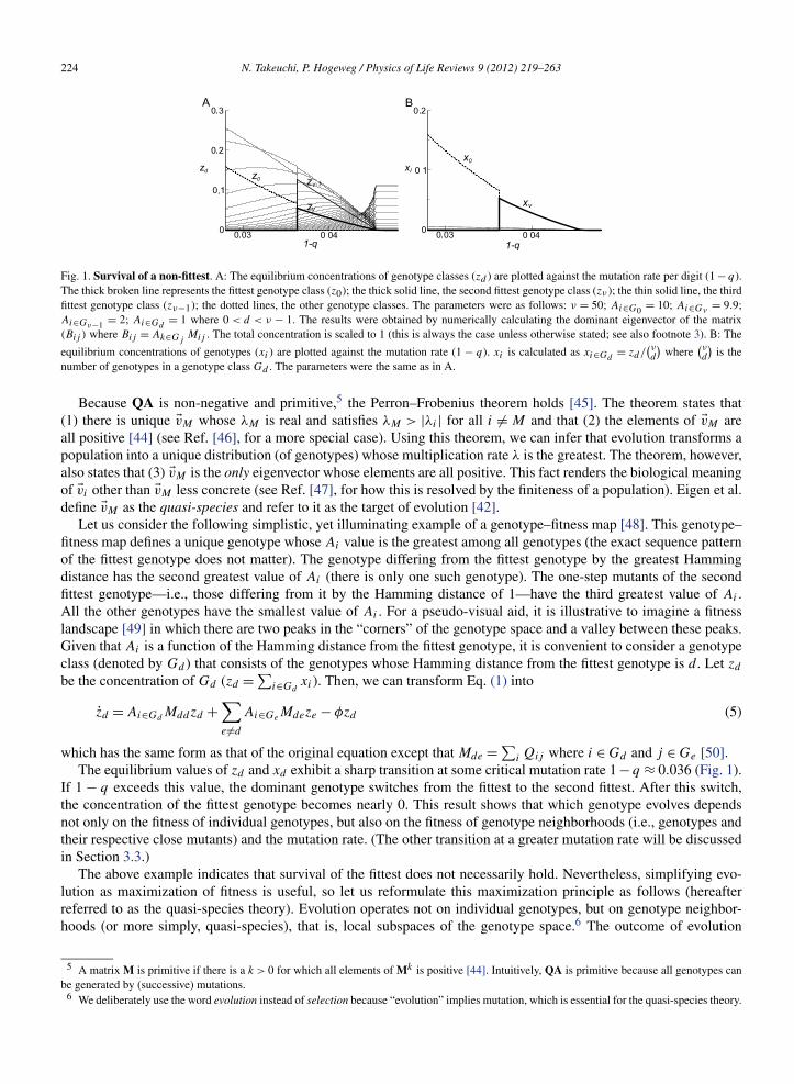


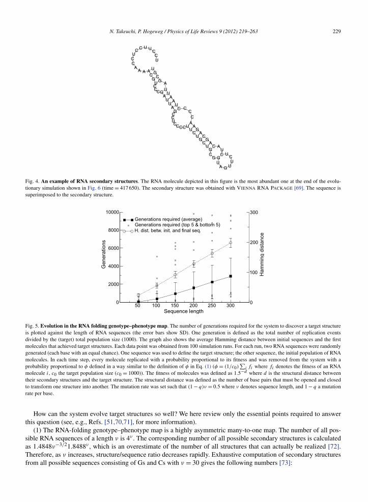
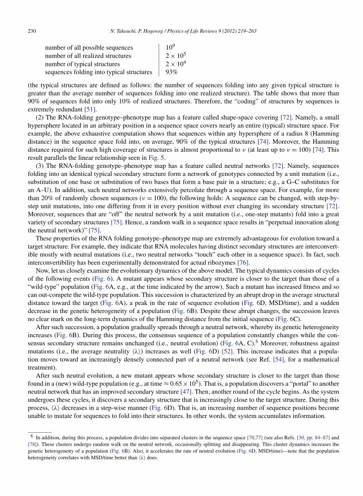


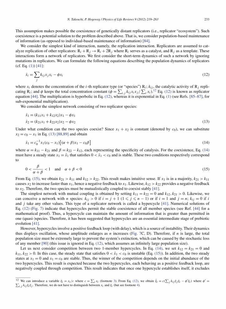

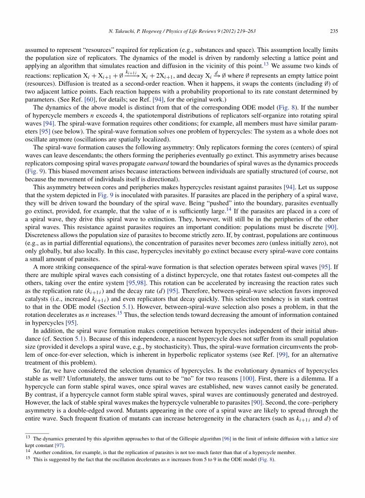


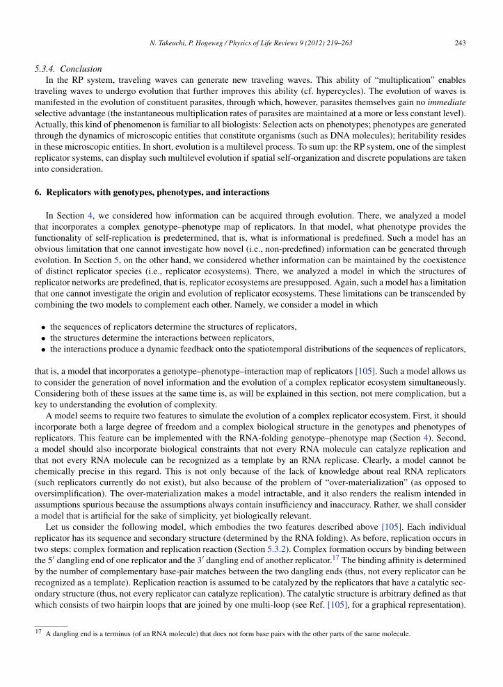


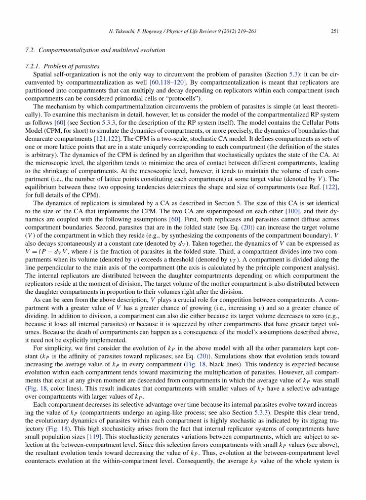


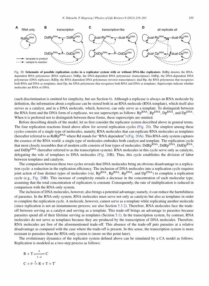
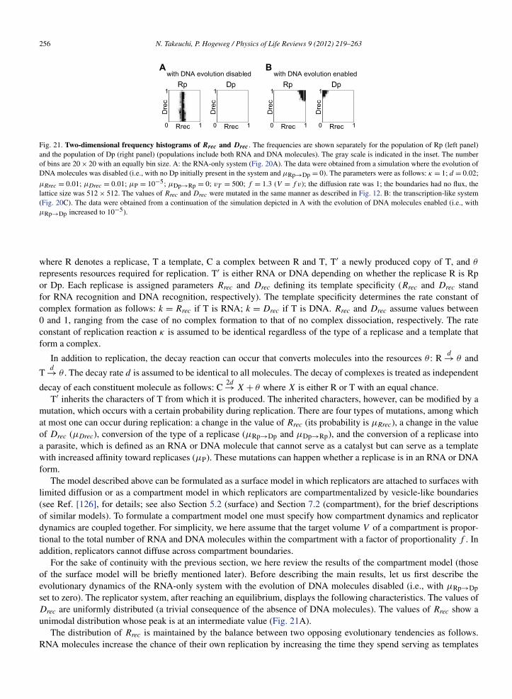
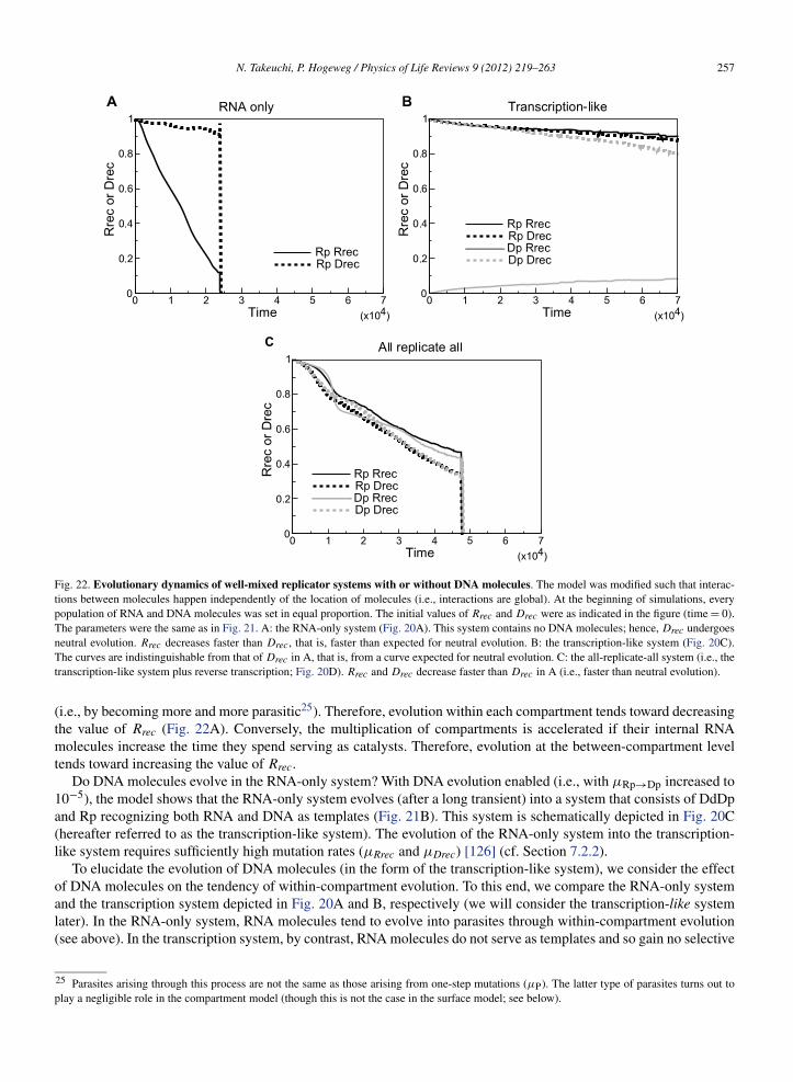

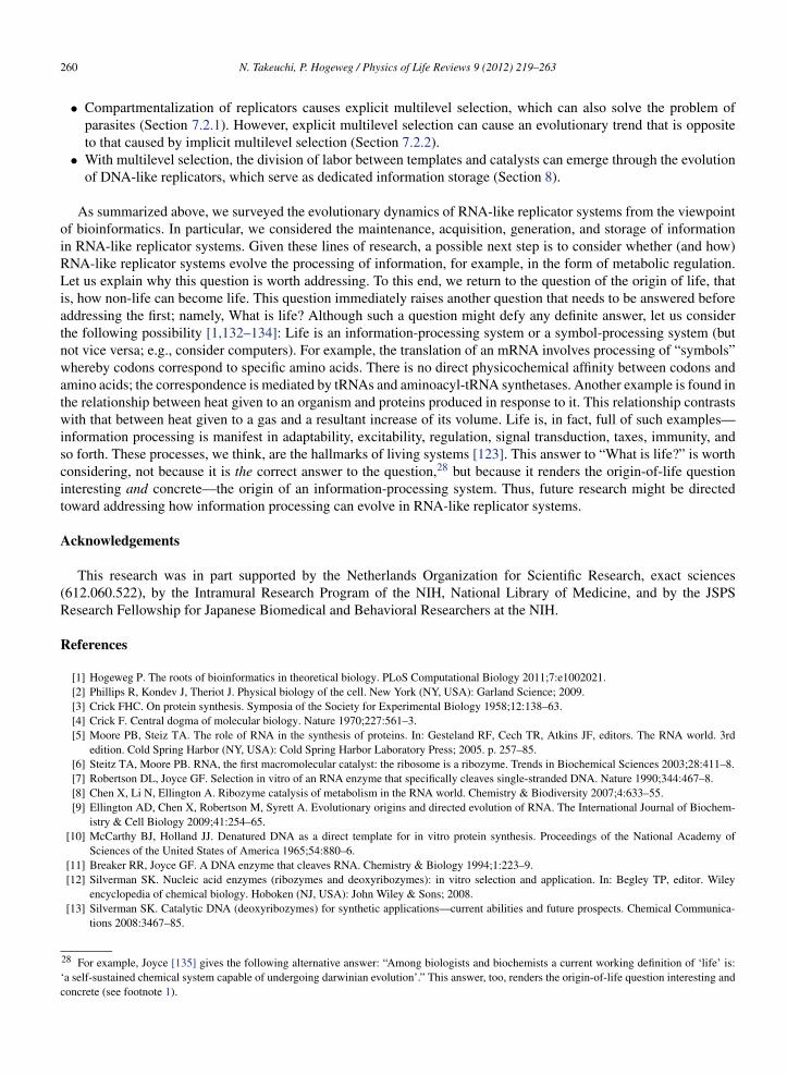


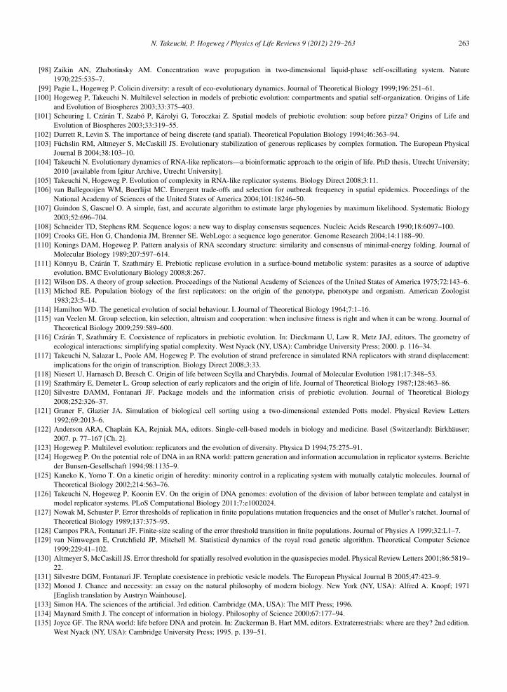


![arXiv:1403.3885v5 [cs.GT] 6 Nov 2015 fileThe golden standard typically is the behavior of learning dynamics in potential games, where many evolutionary dynamics, e.g., replicator,](https://static.documents.pub/doc/80x56/5cb6b59388c9930d3b8ba5c3/arxiv14033885v5-csgt-6-nov-2015-golden-standard-typically-is-the-behavior-of.jpg)


