220


INSTITUTO DE INVESTIGAÇÃO E FORMAÇÃO AVANÇADA
ÉVORA, 2015
ORIENTADORES: Prof.ª Dr.ª Maria Madalena Vitório Moreira Vasconcelos
Prof. Dr. João Alexandre Medina Corte-Real
Tese apresentada à Universidade de Évora
para obtenção do Grau de Doutor em
Ciências da Engenharia do Território e Ambiente
Especialidade: Engenharia Civil
Rong Zhang
INTEGRATED MODELLING FOR EVALUATION OF CLIMATE CHANGE
IMPACTS ON AGRICULTURAL DOMINATED BASIN


Tese de Doutoramento financiada pelo Ministério da Educação e Ciência
Fundação para a Ciência e a Tecnologia
Bolsa de Doutoramento SFRH/BD/48820/2008
Centro de Investigação da Universidade de Évora, de acolhimento da Bolseira


致我父亲和母亲:感谢您们让我的梦想变成了现实
致我叔叔和婶婶:感谢您们永无止境的支持和鼓励
To Professors Cui GuangBai and João Corte-Real:
Thank you for having opened a door to a wonderful world
Ao meu amor Sandro:
Obrigada por fazer parte da minha vida


Acknowledgments
I would like to thank my supervisors, Prof. Madalena Moreira and Prof. João Corte-
Real, for their invaluable guidance and support throughout the period of this research.
This thesis was made possible by a PhD grant of Portuguese national funding agency
for science, research and technology (SFRH/BD/48820/2008). I am very grateful to
Prof. Francisco Sepúlveda Texeira, vice-president of FCT in 2008, and Mrs. Gertrudes
Almeida for the opportunity of fellowship.
I wish to thank the support from the projects ERLAND (PTDC/AAC-AMB/100520/2008),
CLIPE (PTDC/AAC-CLI/111733/2009) and KLIMHIST (PTDC/AAC-CLI/119078/2010),
the observed data from SNIRH, SAGRA/COTR and IPMA and the climate model data
provided by the EU-FP6 project ENSEMBLES.
I am deeply grateful to Prof. Cui Guangbai, my previous supervisor in Hohai University,
China, for his great advice, encouragement and support to the opportunity of this
research.
I very much appreciate the twice opportunities offered by Prof. Chris Kilsby for me to
visit Newcastle University to have training courses on SHETRAN model and
development of weather generator applications. I would like to thank him and his
colleagues, Dr. James Bathurst, Prof. John Ewen, Dr. Stephen Birkinshaw, Dr. Isabella
Bovolo, Prof. Hayley Fowler, Dr. Aidan Burton, Dr. Stephen Blenkinsop, Dr. Greg
O’Donnell and Dr. Nathan Forsythe, for the observed data, great assistance and helpful
discussions.
I would like to thank Prof. Celso Santos and Dr. Paula Freire for their valuable visit to
University of Évora. The collaboration was very helpful and fruitful.
I would further like to thank Prof. Ricardo Serralheiro, Prof. Lúcio Santos, Prof. Elsa
Sampaio, Prof. Shakib Shahidian, Dr. Qian Budong, Dr. Sandra Mourato, Dr. Célia
Toureiro and Dr. Júlio Lima for help, comments and scientific discussions during the
elaboration of this thesis.
I would like to thank my friends at University of Évora, Hohai University and Newcastle
University for making my stay so enjoyable. Special Thanks go to Prof. José Peça,
Regina Corte-Real, Isilda Menezes, Susana Mendes, Luiz Tadeu Silva, Cláudia
Vicente, Clarisse Brígido, Guilhermina Pias, Maria João Vila Viçosa, Ana Canas, Lígia
Justo, Elisete Macedo, Véronica Moreno, Cláudia Furtado, Marco Machado, Amaia
Nogales, Daniel Malet and Lemos Djata.
I want to thank my family for all their love and support. I would like to thank Sandro
Veiga and his family for all the encouragement and support.


i
Integrated Modelling for Evaluation of Climate
Change Impacts on Agricultural Dominated
Basin
Abstract
This study evaluated future climate change impacts on water resources, extreme
discharges and sediment yields for the medium-sized (705-km2) agriculture dominated
Cobres basin, Portugal, in the context of anti-desertification strategies. We applied the
physically-based spatially-distributed hydrological model—SHETRAN, obtaining the
optimized parameters and spatial resolution by using the Modified Shuffled Complex
Evolution (MSCE) method and the Non-dominated Sorting Genetic Algorithm II (NSGA-
II), to simulate the hydrological processes of runoff and sediment transport. We used
the model RanSim V3, the rainfall conditioned weather generator—ICAAM-WG,
developed in this study, based on the modified Climate Research Unit daily Weather
Generator (CRU-WG), and SHETRAN, to downscale projections of change for 2041–
2070, from the RCM HadRM3Q0 with boundary conditions provided by the AOGCM
HadCM3Q0, provided by the ENSEMBLES project, under SRES A1B emission
scenario.
We found future climate with increased meteorological, agricultural and hydrological
droughts. The future mean annual rainfall, actual evapotranspiration, runoff and
sediment yield are projected to decrease by the orders of magnitude of respectively
~88 mm (19%), ~41 mm (11%), ~48 mm (50%) and ~1.06 t/ha/year (45%). We also
found reductions in extreme runoff and sediment discharges, for return periods smaller
than 20 years; however for return periods in the range of 20–50 years, future extremes
are of the same order of magnitude of those in the reference climate.

ii

iii
Modelação integrada para avaliação dos
impactos das alterações climáticas sobre
bacias hidrográficas com uso
predominantemente agrícola
Resumo
Neste estudo são avaliados os impactos futuros das alterações climáticas nos
recursos hídricos e em extremos do escoamento e transporte de sedimentos, na bacia
hidrográfica do rio Cobres, Portugal, agrícola, de dimensão média (705 Km2), no
contexto do combate à desertificação. Foi aplicado o modelo hidrológico fisicamente
baseado e espacialmente distribuído SHETRAN, tendo sido obtidos os valores
optimizados de parâmetros e da resolução espacial, utilizando o método “Modified
Shuffled Complex Evolution” (MSCE) e o algoritmo “Non-dominated Sorting Genetic
Algorithm II” (NSGA-II), para simular os processos hidrológicos de escoamento e
transportes de sedimentos. Foram utilizados o modelo de RainSim V3, o gerador de
tempo ICAAM-WG, desenvolvido neste estudo, baseado no CRU-WG, e o SHETRAN,
para o “downscaling” das projecções climáticas para 2041 – 2070, geradas pelo MRC
HadRM3Q0 com condições de fronteira fornecida pelo MCG HadCM3Q0, projecto
ENSEMBLES, sob o cenário SRES A1B.
O clima futuro é caracterizado por um número crescente de secas meteorológicas,
agrícolas e hidrológicas. Os valores médios anuais da precipitação, evapotranspiração
real, escoamento superficial e transporte de sedimentos, revelam decréscimos com
ordens de grandeza respectivamente de ~88 mm (19%), ~41 mm (11%), ~48 mm
(50%) e ~1.06 t/há/ano (45%). Encontraram-se ainda reduções nos valores extremos
do escoamento superficial e do transporte de sedimentos para períodos de retorno
inferiores a 20 anos; contudo, para períodos de retorno no intervalo 20–50 anos, os
valores extremos futuros apresentam a mesma ordem de grandeza que os relativos ao
período de referência mas mantendo níveis equivalentes para os com 20–50 anos.

iv

v
气候变化对农业为主流域的影响的综合模拟
摘要
水资源短缺和沙漠化是葡萄牙南部地区面临的主要问题。为了给沙漠化防治对策提供科
学依据,本文评估了气候变化对葡萄牙南部以农业为主的科布热斯流域(Cobres,面积约
705 km2)的水资源、暴雨径流和泥沙流失的影响。采用基于物理机制的分布式水文模型
SHETRAN 模拟径流和泥沙迁移的水文过程,并运用 MSCE(Modified Shuffled Complex
Evolution)方法和 NSGA-II(Non-dominated Sorting Genetic Algorithm II)算法优化
模型参数和空间步长.采用奈曼–斯科特时空矩形脉冲(STNSRP)模型 RainSimV3,本研
究开发的基于改进的英国气候研究所(Climate Research Unit)天气发生器(CRU-WG)的
雨控天气发生器 ICAAM-WG,对由 ENSEMBLES 项目提供的基于 SRES A1B 温室气体排放情
景下由全球气候模式 HadCM3Q0 提供边界条件的区域气候模式 HadRM3Q0 所模拟的 2041-
2070 年间的气候变化情景做降尺度分析。结果表明,未来该地区的气象干旱、农业干旱
和水文干旱都有加重趋势。未来平均年降雨、蒸散发量、径流和产沙量预计将比现在分
别减少数量级约 88 毫米(19%)、41 毫米(11%)、48 毫米(50%)和 1.06 吨/公顷/年
(45%)。并且,我们预计重现期在 20 年以下的极端径流和输沙量都将减少,重现期在
20–50 年范围内极端径流和输沙量将保持与基准气候模式相同数量级。

vi

vii
Index
Abstract ........................................................................................................................ i
Resumo ...................................................................................................................... iii
摘要 .............................................................................................................................. v
List of Figures ............................................................................................................ xi
List of Tables............................................................................................................ xix
List of Symbols and Abbreviations ........................................................................ xxi
1. Introduction and Objectives ................................................................................... 1
2. Scientific Background ............................................................................................ 3
2.1 Problems of Southern Portugal...................................................................................... 3
2.2 Hydrological Impacts Assessments .............................................................................. 4
2.3 Problems Involved in the Use of Physically-Based Spatially-Distributed
Hydrological Models ............................................................................................................... 6
3. Cobres Basin ........................................................................................................... 9
3.1 Geographical and Climatological Context .................................................................... 9
3.2 Hydrological Data ........................................................................................................... 10
3.3 Sediment Data ................................................................................................................ 12
4. SHETRAN Modelling System ............................................................................... 15
4.1 Water Flow Component ................................................................................................ 15
4.1.1 Interception and Evapotranspiration Module ...................................................... 15
4.1.2 Overland and Channel Flow Module ................................................................... 16
4.1.3 Variably Saturated Subsurface Module............................................................... 17
4.2 Sediment Transport Component ................................................................................. 18
4.2.1 Hillslope Sediment Transport Module ................................................................. 18
4.2.2 Channel Sediment Transport Module .................................................................. 20
5. Calibration of SHETRAN Model ........................................................................... 23
5.1 Introduction ..................................................................................................................... 23

viii
5.2 Calibration Parameters ................................................................................................. 25
5.3 SHETRAN Model Set-Up.............................................................................................. 25
5.4 The Objective Function ................................................................................................. 29
5.5 Automatic Calibration of SHETRAN Model by MSCE .............................................. 32
5.5.1 The MSCE Optimization Algorithm ...................................................................... 32
5.5.2 MSCE Calibration of SHETRAN Hydrological Parameters .............................. 33
5.6 Multi-Objective Calibration of SHETRAN Model by NSGA-II .................................. 42
5.6.1 The NSGA-II Optimization Algorithm ................................................................... 42
5.6.2 Performance Metrics of NSGA-II Algorithm ........................................................ 44
5.6.3 NSGA-II Calibration of SHETRAN Hydrological Parameters .......................... 45
5.6.4 NSGA-II Calibration of SHETRAN Sediment Parameters................................ 53
5.7 Discussion ....................................................................................................................... 60
6. Impacts of Spatial Scale on the SHETRAN Model .............................................. 63
6.1 Introduction ..................................................................................................................... 63
6.2 Methods and Data ......................................................................................................... 64
6.3 Impacts of Spatial Scale on the SHETRAN Model Input ......................................... 66
6.4 Impacts of Spatial Scale on the SHETRAN Model Performance ........................... 70
6.4.1 Introduction .............................................................................................................. 70
6.4.2 Impacts of Spatial Scale on Long-Term Runoff Simulation ............................. 70
6.4.3 Impacts of Spatial Scale on Storm-Runoff Generation ..................................... 84
6.5 Discussion ....................................................................................................................... 89
7. Downscaling of Climate Change Scenarios ........................................................ 91
7.1 Introduction ..................................................................................................................... 91
7.2 Methodology and Data .................................................................................................. 93
7.2.1 Data Preparation ..................................................................................................... 93
7.2.2 Multi-Site Daily Precipitation Time Series: the RainSim V3 Model ................. 98
7.2.3 Daily Temperature and Evapotranspiration Time Series: the Weather
Generator (ICAAM-WG) Model ...................................................................................... 99
7.2.4 Change Factors Calculation for Future Time Slice 2041–2070 .................... 101
7.2.5 Outline of the Climate Downscaling Method .................................................... 104
7.3 Results of Control Climate Simulations .................................................................... 104
7.3.1 Validation of the RainSim V3 Model .................................................................. 104
7.3.2 Validation of the ICAAM-WG Model .................................................................. 109

ix
7.4 Results of Future Climate Simulations ..................................................................... 111
7.4.1 Simulation of Future Precipitation ...................................................................... 111
7.4.2 Simulation of Future PET .................................................................................... 121
7.5 Discussion ..................................................................................................................... 122
8. Assessment of Future Climate Change Impacts .............................................. 125
8.1 Introduction ................................................................................................................... 125
8.2 Methodology ................................................................................................................. 126
8.2.1 SHETRAN Model Simulation .............................................................................. 126
8.2.2 Statistical Methods ............................................................................................... 127
8.3 Assessment of Future Climate Change Impacts..................................................... 129
8.3.1 Future Climate Change Impacts on Water Availability and Sediment Yield 130
8.3.2 Future Climate Change Impacts on Extreme Events ...................................... 135
8.4 Discussion ..................................................................................................................... 141
9. Conclusions and Expectations .......................................................................... 145
9.1 Summary ....................................................................................................................... 145
9.2 Main Achievements ..................................................................................................... 146
9.3 Main Limitations of the Work ...................................................................................... 147
9.4 Further Research ......................................................................................................... 147
10. References ........................................................................................................ 149
Appendices ............................................................................................................. 163
Appendix 1: Sensitivity Analysis for the SHETRAN Simulation at Cobres Basin with
Spatial Resolution of 2.0 Km and Temporal Resolution of 1.0 Km ............................. 163
Appendix 2: The Proposed Autoregressive Processes in the ICAAM-WG Model ... 166
Appendix 3: Schematic Summary of the Procedure to Downscale the Climate
Change Scenarios. ............................................................................................................. 167
Appendix 4: Plots for Control and Future Rainfall Simulations ................................... 171
Appendix 5: Frequency Distribution of GEV, Gamma and Three-Parameter
Lognormal Distributions ..................................................................................................... 175
A5.1 GEV Distribution: ................................................................................................... 175
A5.2 Gamma Distribution: ............................................................................................. 175
A5.3 Three-Parameter Lognormal Distribution: ......................................................... 175

x

xi
List of Figures
Fig. 3.1 Map showing elevations, gauging stations, rainfall stations and watercourses of the Cobres basin. ....................................................................................................................... 9
Fig. 3.2 Data availability analysis for hourly rainfall series at stations in the Cobres basin (SAO MDA denotes the São Marcos da Ataboeira station). ................................... 11
Fig. 3.3 Double mass curve for monthly rainfall of 6 stations from January 2001 to September 2009. ...................................................................................................................... 11
Fig. 3.4 Plot for comparison between linear and quadratic regressions. ......................... 14
Fig. 5.1 Location map, SHETRAN grid network (abscissa and ordinate indicate grid cell number) and channel system (the heavy blue lines, representing all channel links, and the light blue lines, representing the links used to extract simulated discharges at basin outlet and internal gauging stations) for the Cobres basin, showing the rain gauges (the red circles) and gauging stations (the blue circles at outlet, northern and central parts of the basin, are respectively Monte da Ponte, Albernoa and Entradas gauging stations). The grid squares have dimensions 2 × 2.0 km2. ................................................................. 26
Fig. 5.2 Soil water retention curve for Px soil in Cobres basin (result from MSCE calibration scenario IV). ........................................................................................................... 35
Fig. 5.3 Comparison of observed and simulated discharges from MSCE calibration scenario IV for the Cobres basin with spatial resolution of 2.0 km grid and temporal resolution of 1.0 hour, for main periods of (a) calibration and (b) validation processes.38
Fig. 5.4 Water balance analysis of MSCE calibration scenario IV for calibration and validation periods; P –precipitation, AET – actual evapotranspiration, ΔS – change of subsurface water storage, R – total runoff. .......................................................................... 39
Fig. 5.5 Comparison of observed and simulated discharges from MSCE calibration scenario IV for the Cobres basin with spatial resolution of 2.0 km grid and temporal resolution of 1.0 hour: (a) Storm No.1 at basin outlet; (b) Storm No.4 at basin outlet; (c) Storm No.4 at internal gauging station Albernoa; (d) Storm No.4 at internal gauging station Entradas. ....................................................................................................................... 40
Fig. 5.6 (a) The ensemble of approximation sets obtained from the last generation of the 90 trial runs of NSGA-II algorithm for SHETRAN calibration where RMSE, LOGE and NSE are respectively root mean square errors, log-transformed errors and Nash-Sutcliffe Efficiency. The asterisks in red, blue and light blue colors respectively represent (ηc, ηm) with values (0.5, 0.5), (2.0, 0.5) and (20., 20.). Two-dimensional presentations of figure (a) are shown in (b), (c) and (d). .................................................... 46
Fig. 5.7 (a) The best known approximation sets derived from 30 trial runs of NSGA-II algorithm with (ηc, ηm) of (0.5, 0.5), (2.0, 0.5) and (20., 20.) are respectively shown in small black squares, filled blue circles and filled purplish red circles. The final one derived from all trial runs is shown in filled red circles. (b) The final best known approximation set is made up of solutions from trial runs of NSGA-II algorithm with (ηc, ηm) of (0.5, 0.5) and (2.0, 0.5), respectively showing in filled red and blue circles. The false front, in small black squares, is an example of the approximation set derived from a trapped trial run of the NSGA-II algorithm. ........................................................................ 47

xii
Fig. 5.8 Plots of dynamic performance results of NSGA-II algorithm, namely hypervolume (a, b and c), Ԑ-indicator (d, e and f), generational distance (g, h and i) and opt-indicator (j, k and l), versus total number of SHETRAN model runs. Mean performance is indicated by a solid line, the standard deviation by a dashed line, and the range of performance by the shaded region. The left, middle and right columns of plots were respectively generated from 30 trial runs of NSGA-II with (ηc, ηm) of (0.5, 0.5), (2.0, 0.5) and (20., 20.). .................................................................................................. 48
Fig. 5.9 Plots of dynamic performance results of NSGA-II algorithm, namely hypervolume (a), Ԑ-indicator (b), generational distance (c) and opt-indicator (d), versus total number of SHETRAN evaluations. The 50th and 95th percentiles of performance are respectively indicated in dash and bold solid lines. The red, blue and light blue lines were respectively generated from 30 trial runs of NSGA-II with (ηc, ηm) of (0.5, 0.5), (2.0, 0.5) and (20., 20.). .................................................................................................................... 49
Fig. 5.10 Plots of SHETRAN model performance indicators, namely RMSE, LOGE and NSE, at basin outlet Monte da Ponte (a, d, g and j) and internal gauging stations Albernoa (b, e, h and k) and Entradas (c, f, i and l). The results for the calibration period are denoted by “(calib)” and those for the validation period by “(valid)”. The filled red triangles, blue squares and black circles respectively represent the solutions of best known approximation sets derived from 30 trial runs of NSGA-II with (ηc, ηm) of (0.5, 0.5), (2.0, 0.5) and (20., 20.). ......................................................................................... 50
Fig. 5.11 Comparison between observed and simulated discharges from solutions obtained from automatic calibration of SHETRAN model by NSGA-II algorithm: (a) Storm No.1 at basin outlet; (b) Storm No.4 at basin outlet; (c) Storm No.4 at internal gauging station Albernoa; (d) Storm No.4 at internal gauging station Entradas. “Qsim1”, “Qsim2”, “Qsim3” and “Qsim4” are SHETRAN simulations, for the calibration period (2004-2006), with objective functions (RMSE, LOGE, NSE) at basin outlet of respective values (2.81, 2.74, 0.87), (3.81, 2.53, 0.77), (4.85, 2.49, 0.63) and (5.85, 2.46, 0.46). 52
Fig. 5.12 Comparisons between observed and simulated hourly discharges and sediment discharges for the solution obtained from automatic calibration of sediment parameters by NSGA-II. “Qobs”, “Qsim”, “Qsedobs” and “Qsedsim” respectively represent observed discharge, simulated discharge, observed sediment discharge and simulated sediment discharge. Time is shown in the “MM/DD/YY” format. ...................................... 60
Fig. 6.1 Maps of land-use distribution for Cobres basin with respective spatial resolutions of 0.5, 1.0, 1.5 and 2.0 km. ................................................................................. 67
Fig. 6.2 Maps of soil type distribution for Cobres basin with respective spatial resolutions of 0.5, 1.0, 1.5 and 2.0 km. ................................................................................. 68
Fig. 6.3 Maps of river links distribution for Cobres basin with respective spatial resolutions of 0.5, 1.0, 1.5 and 2.0 km. The red lines represent river links, introduced by the non-standard set-up, developed in the thesis, in the SHETRAN simulations, and the purple ones indicate those provided by SNIRH. .................................................................. 69
Fig. 6.4 Plots showing the comparisons of SHETRAN performances resulting from different spatial discretizations. The black (and light blue), blue and red asterisks represent the ensembles of elite solutions derived from the processes of SHETRAN calibration for Cobres basin with respective spatial resolutions of 2.0, 1.0 and 0.5 km. The subscripts LHS1 and LHSall respectively represent the 1st and all the 30 initial parameter settings generated by the LHS technique. The NSGA-II algorithm with (ηc, ηm) of (0.5, 0.5) was used for calibration. ............................................................................. 71

xiii
Fig. 6.5 The best known approximation sets shown in filled black squares (and filled purplish red circles), filled blue and red circles respectively for spatial discretization schemes of 2.0, 1.0 and 0.5 km. The subscripts LHS1 and LHSall respectively represent the 1st and all the 30 initial parameter settings generated by the LHS technique. The NSGA-II algorithm with (ηc, ηm) of (0.5, 0.5) was used for calibration. . 72
Fig. 6.6 Plots of dynamic performance results of NSGA-II algorithm, namely hypervolume (a), Ԑ-indicator (b), generational distance (c) and opt-indicator (d), versus total number of SHETRAN evaluations. The black (grey shadow area), blue and red solid lines refer to respective spatial discretization schemes of 2, 1.0 and 0.5 km. The subscripts LHS1 and LHSall respectively represent the 1st and all the 30 initial parameter settings generated by the LHS technique. ........................................................ 73
Fig. 6.7 Plots of SHETRAN model performance indicators, namely RMSE, LOGE and NSE, at basin outlet Monte da Ponte (a, d, g and j) and internal gauging stations Albernoa (b, e, h and k) and Entradas (c, f, i and l). The results for the calibration period (2004‒2006) are denoted by “(calib)” and those for the validation period (2006‒2008) by “(valid)”. The filled red triangles and blue squares represent the solutions with NSE values higher or equal to 0.85, for calibration, derived respectively from the spatial discretization schemes of 1.0 and 2.0 km. The subscript LHS1 represents the 1st initial parameter setting generated by the LHS technique. .......................................................... 79
Fig. 6.8 Plots of SHETRAN model performance indicators, namely RMSE, LOGE and NSE, at basin outlet Monte da Ponte gauging station. The results are for the validation period 1977‒1979. The filled red triangles and blue squares represent the solutions with NSE values higher or equal to 0.85, for calibration, derived respectively from the spatial discretization schemes of 1.0 and 2.0 km. The subscript LHS1 denotes the initial parameter setting used in model calibration. ............................................................. 80
Fig. 6.9 Plots of SHETRAN model performance indicators, namely RMSE, LOGE and NSE, at basin outlet Albernoa (a, c, e and g) and internal gauging station Entradas (b, d, f and h). The results for the validation period (2004‒2006) are denoted by “(valid2004to06)” and those for the validation period (2006‒2008) by “(valid2006to08)”. The filled red triangles and blue squares represent the solutions with NSE values higher or equal to 0.85, for SHETRAN calibration, at Cobres basin with respective spatial resolutions of 1.0 and 2.0 km. The subscript LHS1 denotes the initial parameter setting used in model calibration. ........................................................................................... 80
Fig. 6.10 Comparisons of observed and simulated hourly discharges from the SHETRAN calibrations for Cobres basin with respective spatial resolutions of 2.0 and 1.0 km during the main periods of simulations. ................................................................... 82
Fig. 6.11 Plots of monthly precipitation (P), potential evapotranspiration (PET) and runoff (R) for the calibration period 2004‒2006 (a), the validation periods 2006‒2008 (b) and 1977‒1979 (c). .................................................................................................................. 83
Fig. 6.12 Comparisons of accumulated monthly runoff at Monte da Ponte gauging station between observations (OBS) and the simulations by SHETRAN model, with respective spatial resolutions of 2.0 km (2kmLHS1) and 1.0 km (1kmLHS1), shown in thick black and normal red and blue lines. For the spatial discretization schemes of 1.0 and 2.0 km, the 8 and 25 solutions with values of NSE higher or equal to 0.85, for calibration, are displayed; for SHETRAN calibration, the NSGA-II algorithm with (ηc, ηm) of (0.5, 0.5) and initial parameter setting of LHS1 was used. ............................................ 84

xiv
Fig. 6.13 NSE indicators for the SHETRAN simulations of the storms No.1, 4, I, II, III, IV, V, VI, VII, VIII and IX at Cobres basin with spatial resolutions of 1.0 and 2.0 km respectively shown in red and blue filled circles. The abscissa tick marks of 4, 4a and 4e are for storm No.4, showing results respectively evaluated at basin outlet and internal gauging stations Albernoa and Entradas; the others are for the respective storms evaluated at basin outlet. For the spatial discretization schemes of 1.0 and 2.0 km, the 8 and 25 solutions with values of NSE higher or equal to 0.85, for calibration, are displayed; for SHETRAN calibration, the NSGA-II algorithm with (ηc, ηm) of (0.5, 0.5) and initial parameter setting of LHS1 was used. ................................................................. 85
Fig. 6.14 MBE and PKE indicators for the SHETRAN simulations of the storms No.1, 4, I, II, III, IV, V, VI, VII, VIII and IX at Cobres basin with spatial resolutions of 1.0 and 2.0 km respectively shown in filled red and blue circles. .......................................................... 86
Fig. 6.15 Observed and simulated discharges from the SHETRAN calibrations by the NSGA-II algorithm with (ηc, ηm) of (0.5, 0.5) for the Cobres basin with spatial resolutions of 2.0 and 1.0 km: (a) Storm No.1 at basin outlet; (b) Storm No.4 at basin outlet; (c) Storm No.4 at internal gauging station Albernoa; (d) Storm No.4 at internal gauging station Entradas. ....................................................................................................................... 87
Fig. 6.16 Observed and simulated discharges at basin outlet from the SHETRAN calibrations by the NSGA-II algorithm with (ηc, ηm) of (0.5, 0.5) for the Cobres basin with spatial resolutions of 2.0 and 1.0 km: (a) Storm No.I; (b) Storm No.II; (c) Storm No.III and (d) Storm No.IV. ..................................................................................................... 88
Fig. 6.17 Observed and simulated discharges at basin outlet from the SHETRAN calibrations by the NSGA-II algorithm with (ηc, ηm) of (0.5, 0.5) for the Cobres basin with spatial resolutions of 2.0 and 1.0 km: (a) Storm No.V; (b) Storm No.VI; (c) Storm No.VII; (d) Storm No.VIII and (e) Storm No.IX. .................................................................... 89
Fig. 7.1 Location map of the Cobres basin with climatological station (black triangle), rain gauges (blue dots) and the selected regional climate model grid cells’ centers (red circles) ........................................................................................................................................ 95
Fig. 7.2 Annual cycles of mean daily precipitation (Pbej), potential evapotranspiration (PETbej), daily maximum (Tmaxbej) and daily minimum 2-m air temperature (Tminbej) for Beja station, mean daily precipitation for each station (Pcobstatns), and basin average precipitation (Pcobavg) at Cobres basin. All are derived from the observations over the period from 1981–2010 except PETbej, which is from 1981–2004. ................................... 96
Fig. 7.3 Relationships between hourly and daily rainfall statistics, (a) variance, (b) skewness and (c) proportion dry, derived from pairs of the monthly statistics of the 62 stations located in the Guadiana basin (744 observed statistics). The 84 observed statistics, shown in red filled circles, are for the 7 stations of the Cobres basin located in the Guadiana basin .............................................................................................................. 97
Fig. 7.4 Annual cycles of CFs for (a) mean MDP, (b) variance VarDP, (c) skewness SkewDP, (d) transformed proportion of dry days X(PdryDP1.0) and (e) transformed lag-1 autocorrelation Y(L1ACDP) of daily rainfall, (f) mean MDT and (g) variance VarDT of daily mean temperature and (h) mean M∆T and (i) variance Var∆T of daily temperature range, for the 6 RCM grid cells overlying Cobres basin; the average CF, shown in red colour, is the average of CFs from the 6 RCM grid cells. .............................................................. 103
Fig. 7.5 Comparison of the annual cycles of observed (solid lines), fitted (circles) and simulated (crosses) daily (a1, a2 and a3) mean, (b1, b2 and b3) variance, (c1, c2 and c3)

xv
skewness, (d1, d2 and d3) proportion of dry days and (e1, e2 and e3) lag-1 autocorrelation and hourly (f1, f2 and f3) variance, (g1, g2 and g3) skewness and (h1, h2 and h3) proportion dry hours during the control period (1981−2010) for the 7 rain gauges at the Cobres basin with each colour representing one site. The first (Figs. a1, b1, c1, d1, e1, f1, g1 and h1), second (Figs. a2, b2, c2, d2, e2, f2, g2 and h2) and third (Figs. a3, b3, c3, d3, e3, f3, g3 and h3) column of figures respectively represents results from the 1st, 2nd and 3rd 1000-year synthetic hourly rainfall. ............................................................ 107
Fig. 7.6 Observed (solid blue lines), fitted (red circles) and simulated (black crosses) cross-correlations against separation for January (a1, a2 and a3) and July (b1, b2 and b3). The first (Figs. a1 and b1), second (Figs. a2 and b2) and third (Figs. a3 and b3) columns respectively represent results from the 1st, 2nd and 3rd series of 1000-year synthetic hourly rainfall. .......................................................................................................................... 108
Fig. 7.7 Validation of weather generator (ICAAM-WG) for simulated daily (a) maximum temperature (Tmax), (b) minimum temperature (Tmin) ), (c) vapour pressure (VP), (d) wind speed (WS), (e) sunshine duration and (f) potential evapotranspiration (PET) at Beja station during the control period (1981–2010); the circles indicate the observed weather statistics, the crosses represent the simulated means of corresponding values and the error bars represent variability denoted by two standard deviations of the simulated 100 annual means. ............................................................................................... 112
Fig. 7.8 Annual cycles of daily (a1, a2 and a3) mean, (b1, b2 and b3) variance, (c1, c2 and c3) skewness, (d1, d2 and d3) proportion of dry days and (e1, e2 and e3) lag-1 autocorrelation and hourly (f1, f2 and f3) variance, (g1, g2 and g3) skewness and (h1, h2 and h3) proportion dry hours for precipitation at the Beja station from the three 1000-year simulations of the future period (2041–2070) compared to the control period (1981–2010). The observed (OBS) or projected (PRJ), fitted (EXP) and simulated (SIM) statistics are respectively shown in solid lines, circles and crosses and in respective colors of blue and red for the control (CTL) and future (FUT) periods. .......................... 114
Fig. 7.9 Annual cycles of daily (a1, a2 and a3) mean, (b1, b2 and b3) variance, (c1, c2 and c3) skewness, (d1, d2 and d3) proportion of dry days and (e1, e2 and e3) lag-1 autocorrelation and hourly (f1, f2 and f3) variance, (g1, g2 and g3) skewness and (h1, h2 and h3) proportion dry hours for precipitation at the Castro verde station from the three 1000-year simulations of the future period (2041–2070) compared to the control period (1981–2010). The observed (OBS) or projected (PRJ), fitted (EXP) and simulated (SIM) statistics are respectively shown in solid lines, circles and crosses and in respective blue and red colors for the control (CTL) and future (FUT) periods. .............................. 116
Fig. 7.10 Gumbel plots comparing observed and simulated extreme daily rainfall for (a) Beja, (b) Castro verde, (c) Almodôvar and (d) Trindade. The observed rainfall, shown in black solid squares, is for 1961–2010 at Beja station provided by IPMA and for 1931−2011 at stations Castro Verde, Almodôvar and Trindade provided by SNIRH; the simulated rainfall was generated by the RainSim V3 model, shown in respective blue and red solid lines for the control (1981−2010) and future (2041−2070) periods. ....... 119
Fig. 7.11 Comparison of the annual cycless of observed (1981–2010: blue circles) and future (1981–2010: red crosses, black circles) daily (a) maximum temperature (Tmax) and (b) minimum temperature (Tmin), (c) vapour pressure (VP), (d) wind speed (WS), (e) sunshine duration (SS) and (f) potential evapotranspiration (PET) at Beja station; the circles indicate the observed or expected future weather statistics, the crosses represent the simulated means of corresponding values and the error bars represent variability denoted by two standard deviations of the simulated 100 annual means. .. 122

xvi
Fig. 8.1 Boxplots showing the annual cycles of monthly rainfall (a), PET (b), change of subsurface storage (∆S) (c), AET (d), runoff (e) and sediment yield (f) under control (blue) and future (red) climate conditions. The small circles embedded with black dots represent the median value for each month, the lower (upper) limits of the compacted boxes represent the first quartile q0.25 (third quartile q0.75), the lower (upper) limits of the whiskers represent the “q0.25 – 1.5 × (q0.75 – q0.25)” (“q0.75 + 1.5 × (q0.75 – q0.25)”) and the circles below the lower whiskers (above the upper whiskers) represent outliers. . 131
Fig. 8.2 Flow duration curves derived from the three 1000-year SHETRAN hydrological simulations under the (a) control and (b) future conditions, which are shown in blue, green, black, purplish-red and red colors respectively for the whole year, autumn, winter, spring and summer. Comparisons are shown in (c), (d), (e) and (f), with blue representing control and red for future, respectively for the whole year, autumn, winter and spring. The abscissa shows the percentage of flow exceeded and the ordinate indicates flows at outlet of the Cobres basin in a natural log-scale. ............................... 134
Fig. 8.3 Gumbel plots comparing annual maximum daily (a) discharge and (b) sediment discharge for Monte da Ponte gauging station (basin outlet) in blue and red colors respectively under control (1981−2010) and future (2041−2070) conditions. 5%, 50% and 95% represent the 5th, 50th and 95th percentile of the extremes. ............................. 135
Fig. 8.4 Empirical cumulative frequency distribution functions for (a) the annual maximum daily discharge and (c) the annual maximum daily sediment discharge under control (CTL) and future (FUT) conditions. Empirical extreme plots for comparison of (b) annual maximum daily discharge and (d) annual maximum daily sediment discharge under control and future conditions. The 3000-year synthetic daily discharge and sediment discharge series were used to derive the plots. ............................................... 137
Fig. 8.5 Probability distributions of annual maximum daily discharge under (a) control and (b) future conditions and annual maximum daily sediment discharge under (c) control and (d) future conditions. The red circles are derived from SHETRAN model simulations; the blue and black lines are fitted, by using the R functions of the lmom package (version 2.1), based on postulated distributions, namely generalized extreme value (GEV), Gumbel or extreme value (EV), gamma and three-parameter lognormal (ln3) distributions. The blue lines are corresponding best fits. ........................................ 138
Fig. 8.6 L-moment diagram indicating relationships among L-skewness and L-Kurtosis for the generalized logistic (GLO), generalized extreme value (GEV), generalized Pareto (GPA), generalized normal (GNO), Pearson type III (PE3), exponential (E), Gumbel (G), logistic (L), normal (N) and uniform (U) and the distribution of the 3000-year annual maximum daily discharge under control (blue circle) and future (red circle) conditions and the 3000-year annual maximum daily sediment discharge under control (blue cross) and future (red cross) conditions. .................................................................. 139
Fig. 8.7 Histograms of fitted distributions for (a) annual maximum daily discharge and (b) annual maximum daily sediment discharge under control (CTL) and future (FUT) conditions. ................................................................................................................................ 140
Fig. A3.1 Schematic chart of validation of the RainSim V3 model with numbering corresponding to the steps directed in black arrows. ........................................................ 167
Fig. A3.2 Schematic chart of future rainfall simulation by using the RainSim V3 model with numbering corresponding to the steps directed in black arrows............................. 168

xvii
Fig. A3.3 Schematic chart of validation of the ICAAM-WG model with numbering corresponding to the steps directed in black arrows. ........................................................ 169
Fig. A3.4 Schematic chart of future PET simulation by using the ICAAM-WG model with numbering corresponding to the steps directed in black arrows. .................................... 170
Fig. A4.1 Annual cycles of daily (a1, a2 and a3) mean, (b1, b2 and b3) variance, (c1, c2 and c3) skewness, (d1, d2 and d3) proportion of dry days and (e1, e2 and e3) lag-1 autocorrelation and hourly (f1, f2 and f3) variance, (g1, g2 and g3) skewness and (h1, h2 and h3) proportion dry hours for precipitation at the Almodôvar station from the three 1000-year simulations of the future period (2041–2070) compared to the control period (1981–2010). The observed (OBS) or projected (PRJ), fitted (EXP) and simulated (SIM) statistics are respectively shown in solid lines, circles and crosses and in respective blue and red colors for the control (CTL) and future (FUT) periods. .............................. 172
Fig. A4.2 Annual cycles of daily (a1, a2 and a3) mean, (b1, b2 and b3) variance, (c1, c2 and c3) skewness, (d1, d2 and d3) proportion of dry days and (e1, e2 and e3) lag-1 autocorrelation and hourly (f1, f2 and f3) variance, (g1, g2 and g3) skewness and (h1, h2 and h3) proportion dry hours for precipitation at the Trindade station from the three 1000-year simulations of the future period (2041–2070) compared to the control period (1981–2010). The observed (OBS) or projected (PRJ), fitted (EXP) and simulated (SIM) statistics are respectively shown in solid lines, circles and crosses and in respective blue and red colors for the control (CTL) and future (FUT) periods. .............................. 174

xviii

xix
List of Tables
Table 3.1 Available TSS, turbidity and hourly discharge at Monte da Ponte gauging station ......................................................................................................................................... 13
Table 3.2 Summary statistics for the data sets shown in Table 3.1 ................................. 14
Table 5.1 Comparison of model performances from manual and MSCE calibrations at basin outlet (Monte da Ponte gauging station) .................................................................... 29
Table 5.2 Description of SHETRAN key hydrological parameters, feasible ranges, baseline setting (in bracket) and values derived from manual and MSCE calibrations for different scenarios (I, II, III and IV) as explained in the Section 5.5.2 .............................. 31
Table 5.3 Comparison of model performances from manual and MSCE calibrations at basin outlet (Monte da Ponte gauging station) .................................................................... 36
Table 5.4 Statistics for the MSCE calibration scenario IV at Cobres basin ..................... 37
Table 5.5 Vegetation parameters for sediment transport simulations of Cobres basin . 54
Table 5.6 Soil textural data from Cardoso (1965) for soil types in Cobres basin ........... 54
Table 5.7 Soil particle-size distribution for soil types in Cobres basin ............................. 55
Table 5.8 Mass fraction for sediment particle-size distribution of soil types in Cobres basin ........................................................................................................................................... 55
Table 5.9 Preliminary sediment simulations of Cobres basin for the period from October, 2004 to November, 2006 ......................................................................................................... 57
Table 5.10 Statistics of annual rainfall and runoff at Cobres basin .................................. 58
Table 6.1 Area, total river length and drainage density of the Cobres basin .................. 69
Table 6.2 The SHETRAN key hydrological parameters derived from calibrations at Cobres basin with spatial resolution of 1.0 km and 2.0 km ................................................ 75
Table 6.3 Comparison of the model performances for the SHETRAN simulations at Cobres basin with spatial resolutions of 1.0 km and 2.0 km .............................................. 81
Table 6.4 Comparison of model performances for SHETRAN validation simulations at Albernoa basin with spatial resolutions of 1.0 km and 2.0 km ........................................... 83
Table 6.5 Observed characteristics of the 11 selected “large storm events” at Cobres basin ........................................................................................................................................... 85
Table 7.1 Characteristics of the stations located in the study area .................................. 94
Table 7.2 The Regional Climate Model (RCM) experiment used from the RT3 ENSEMBLES ............................................................................................................................ 98

xx
Table 7.3a Climate change impacts on moderate precipitation extreme indices (5th percentile) ................................................................................................................................ 119
Table 7.3b Climate change impacts on moderate precipitation extreme indices (50th percentile) ................................................................................................................................ 120
Table 7.3c Climate change impacts on moderate precipitation extreme indices (95th percentile) ................................................................................................................................ 120
Table 7.3d Climate change impacts on moderate precipitation extreme indices (98th percentile) ................................................................................................................................ 120
Table 8.1 Statistics for evaluation of climate change impacts on catchment: average changes in mean, standard deviation (STD), coefficient of variation (CV), 5th, 50th, 95th 98th and 99th percentiles (q0.05, q0.50, q0.95, q0.98 and q0.99) for annual rainfall (P), PET, AET, subsurface storage (∆S), runoff (R) and sediment yield (SY) ............................... 130
Table 8.2a Lilliefors test for annual maximum daily discharge under CTL and FUT conditions ................................................................................................................................. 141
Table 8.2b Filliben test for annual maximum daily discharge under CTL and FUT conditions ................................................................................................................................. 141
Table 8.3a Lilliefors test for annual max daily sediment discharge under CTL and FUT conditions ................................................................................................................................. 141
Table 8.3b Filliben test for annual max daily sediment discharge under CTL and FUT conditions ................................................................................................................................. 141
Table A1.1 Description of SHETRAN key hydrological parameters for the simulations of the baseline and scenarios for sensitivity analysis ............................................................ 164
Table A1.2 Comparison of model performances from the SHETRAN simulations of the baseline and scenarios, with key parameters indicated in the Table A1.1 .................... 165

xxi
List of Symbols and Abbreviations
List of Symbols
a Coefficient of the Yalin equation
A Flow cross sectional area (m2)
AET Actual Evapotranspiration (mm) or (mm/s)
AETPETFC1 The AET/PET ratio at field capacity for crop
AETPETFC2 The AET/PET ratio at field capacity for agroforestry
AII Average dry day precipitation (DP < 10 mm) (mm)
α van Genuchten α parameter (cm-1)
α1 van Genuchten α parameter of Vx soil (cm-1)
α2 van Genuchten α parameter of Px soil (cm-1)
α3 van Genuchten α parameter of Ex soil (cm-1)
αg,i Change factor for the statistic g and the calendar month i
αT,i Change factor for the temperature statistic T and the calendar
month i
b Drainage parameter
B Channel flow width (m) or active bed width for which there is
sediment transport (m)
ci Sediment concentration in size group i (m3/m3)
cP Specific heat of air at constant pressure (J/kg/K)
C Depth of water on canopy (mm)
CDD Maximum number of consecutive dry days (DP < 1.0 mm) (day)
Cc Percentage canopy cover (%)
Cg Proportion of ground shielded by near ground cover (decimal
fraction) or percentage ground cover (%)
Cr Proportion of ground shielded by ground level cover (decimal
fraction)
CR Storm runoff coefficient (%)
D50 Sediment particle diameter greater than the diameter of 50% of
the particles (m);
Dn The largest absolute difference between empirical and fitted
cumulative probabilities
δ Coefficient of the Yalin equation
δe Vapour pressure deficit of air (Pa)

xxii
Δ Rate of increase with temperature of the saturation vapour
pressure of water at air temperature (Pa/K)
ΔS Change of subsurface water storage (mm)
Di Representative sediment particle diameter for the size group i
(m).
DP Daily precipitation (mm)
Dq Rate of detachment of soil per unit area (kg/m2/s)
Dr Rate of detachment of soil (kg/m2/s);
ei White noise on the day i for the equations 7.10─7.24 and
A2.1─A2.13
η Storage coefficient (m-1)
ηc Crossover distribution index
ηm Mutation distribution index
Eb Rate of detachment of material per unit area of river bank
(kg/m2/s)
Ex Lithosols from semi-arid and sub-humid climate of Schist or
Greywacke origin
FDD Number of dry spells (consecutive period with at least 8 dry days,
DP < 1.0 mm) (freq.)
ηc Crossover distribution index
ηm Mutation distribution index
ϕ Bed sediment porosity (m3/m3)
Fw Effect of surface water layer in protecting the soil from raindrop
impact (dimensionless)
g Acceleration due to gravity (m/s2)
γ Psychrometric constant (~66 Pa/K)
𝑔𝑖𝐹𝑢𝑡, 𝑔𝑖
𝐶𝑜𝑛 The statistic g for the calender month i under the future (Fut) and
control (Con) conditions
𝑔𝑖𝑂𝑏𝑠, 𝑔𝑖
𝐸𝑠𝑡 The observed (Obs) and estimated (Est) statistic g for the calender
month i
Ggr,i Dimensionless sediment transport rate for sediment size group i
Gi Volumetric sediment transport rate for particles in size group i
(m3/s)
Gtot The capacity particulate transport rate for overland flow (including
all sediment size groups) (m3/s)
gx, gy Volumetric sediment transport rates per unit width in the x and y
directions respectively (m3/s/m)

xxiii
h Water depth (m) or top soil depth (m)
H Flow depth of channel flow (m)
HP Hourly precipitation (mm)
Imean Mean rainfall intensity (mm/h)
Imax Max rainfall intensity (mm/h)
k Drainage parameter
kb Bank erodibility coefficient (kg/m2/s)
kf Overland flow soil erodibility coefficient (kg/m2/s)
kr Raindrop impact soil erodibility coefficient (J-1) or relative
hydraulic conductivity (-)
K1 (m1/3/s) Strickler overland flow resistance coefficient for crops
K2 (m1/3/s) Strickler overland flow resistance coefficient for agroforestry
Ks Saturated hydraulic conductivity (m/day)
Ks1 Saturated hydraulic conductivity of Vx soil (m/day)
Ks2 Saturated hydraulic conductivity of Px soil (m/day)
Ks3 Saturated hydraulic conductivity of Ex soil (m/day)
Kx, Ky and Kl Strickler coefficients (m1/3/s), which are the inverse of the
Manning coefficient, in the x, y and l directions
Kx, Ky and Kz Saturated hydraulic conductivities in the x, y and z directions (m/s)
l Width of the flow (m)
L1ACDP Lag-1 autocorrelation (-)
λ Loose sediment porosity (decimal fraction) or latent heat of
vaporization of water (J/g)
Md Momentum squared of leaf drips reaching the ground per unit
time per unit area (kg2/s3)
MDP Daily mean rainfall for a specified month (mm)
MDT Mean of daily mean 2-m air temperature for a specified month
(°C)
M∆DT Mean of daily 2-m air temperature range for a specified month
(°C)
Mr Momentum squared of raindrops reaching the ground per unit
time per unit area (kg2/s3)
n Porosity (m3/m3) or van Genuchten n parameter (-)
n1 van Genuchten n parameter of Vx soil (-)
n2 van Genuchten n parameter of Px soil (-)
n3 van Genuchten n parameter of Ex soil (-)

xxiv
ni The transition exponent for sediment size group i for the Ackers-
White equation for Channel flow sediment transport
Oi Observed watershed responses at time point i
�̅� The mean values of observed watershed responses
PET Potential Evapotranspiration (mm)
Ψ Soil moisture tension (m)
Ψw Soil moisture tension at wilting point (m)
ΨL Soil moisture tension at which soil water begins to limit plant
growth and water uptake is considered to take place at the
potential rate (m)
P Precipitation (mm) or non-exceedance probabilities (-)
PdryDP1.0 Proportion of dry days (less than 1.0 mm) (-)
PdryHP0.1 Proportion of dry hours (less than 0.1 mm) (-)
Pi Daily precipitation (mm) for the day i
Pobs Observed precipitation (mm)
Px Brown Mediterranean soil of Schist or Greywacke origin
q Specific volumetric flow rate out of the medium (s-1)
qsi Sediment input from bank erosion and overland flow supplies per
unit channel length for size fraction i (m3/s/m)
qw, qsp and qt Specific volumetric fluxes (s-1) out of abstraction well, spring
discharges and transpiration losses respectively
Q Net rate of rainfall supply to canopy (mm/hour) or water flow rate
(m3/s)
Qb Baseflow ( at the start of the flood) (m3/s)
Qi Lateral influx (m3/s)
Qobs Observed discharge (m3/s)
Qp Peakflow (maximum peakflow for processes with multiple peaks)
(m3/s)
QR Net vertical input to the element (m3/s)
Qobs Observed discharge (m3/s)
Qsim Simulated discharge (m3/s)
𝑄𝑜𝑏𝑠𝑝𝑘
Observed peak discharges (m3/s)
𝑄𝑠𝑖𝑚𝑝𝑘
Simulated peak discharges (m3/s)
ra Aerodynamic resistence to water vapour transport (s/m)
rc Canopy resistance to water vapour transport (s/m).
ρ Water density (kg/m3) or density of air (kg/m3)

xxv
ρs Density of sediment particles (kg/m3)
R Daily 2-m air temperature range (°C) or runoff (mm) or Pearson
correlation coefficient (-)
R5D Highest consecutive 5-day precipitation total (mm)
R30 Number of days with daily precipitation totals above or equal to
30 mm (day)
Ri Daily 2-m air temperature range for the day i (°C)
Rn Net radiation (W/m2)
Robs Observed runoff (mm)
Rsim Simulated runoff (mm)
s Sediment specific gravity (decimal fraction)
S Water surface slope in the direction of flow (m/m) or canopy
storage capacity (mm)
Si Simulated watershed responses at time point i
𝑆̅ The mean values of simulated watershed responses
SDII Average wet day precipitation (DP >= 1.0 mm) (mm)
Sfx, Sfy and Sfl Friction slopes in the x, y and l directions respectively (m/m)
σe Standard deviation of the white noise on the day i for the
equations 7.10─7.24 and A2.1─A2.13
SkewDP Skewness of daily rainfall for a specified month (-)
SkewHP Skewness of hourly rainfall for a specified month (-)
Ss Specific storage (m-1)
SS Sunshine duration (hours)
SSi Sunshine duration for the day i (hours)
SY Sediment Yield (t ha-1 year-1)
t Time (hour or second)
T Daily mean 2-m air temperature (°C) or return period (year)
θ Volumetric soil water content (m3/m3)
θs Saturated soil water content (m3/m3)
θs1 Saturated soil water content of Vx soil (m3/m3)
θs2 Saturated soil water content of Px soil (m3/m3)
θs3 Saturated soil water content of Ex soil (m3/m3)
θr Residual soil water content (m3/m3)
θr1 Residual soil water content of Vx soil (m3/m3)
θr2 Residual soil water content of Px soil (m3/m3)
θr3 Residual soil water content of Ex soil (m3/m3)
Ti Daily mean 2-m air temperature for the day i (°C)

xxvi
𝑇𝑖𝐹𝑢𝑡, 𝑇𝑖
𝐶𝑜𝑛 The temperature statistic T for the calender month i under the
future (Fut) and control (Con) conditions
𝑇𝑖𝑂𝑏𝑠, 𝑇𝑖
𝐸𝑠𝑡 The observed (Obs) and estimated (Est) temperature statistic T for
the calender month i
Tmax Daily maximum 2-m air temperature (°C)
Tmin Daily minimum 2-m air temperature (°C)
τ Shear stress due to overland flow (N/m2)
τb Shear stress acting on the bank (N/m2);
τbc Critical shear stress for initiation of motion of bank material (N/m2)
τec Critical shear stress for initiation of sediment motion (N/m2)
TSS Total suspended solid (mg/l)
Turb Turbidity (NTU)
ux, uy and ul Flow velocities in the x, y and l directions (m/s)
u* Shear velocity of channel flow (m/s)
U Water velocity of channel flow (m/s)
VarDP Variance of daily rainfall for a specified month (mm2)
VarDT Variance of daily mean 2-m air temperature for a specified month
(°C2)
Var∆DT Variance (Var∆DT) of daily 2-m air temperature range for a
specified month (°C2)
VarHP Variance of hourly rainfall for a specified month (mm2)
VP Vapour pressure (kPa)
VPi Vapour pressure for the day i (kPa)
Vx Yellow Mediterranean soil of Schist origin
WS Wind speed (m/s)
WSi Wind speed for the day i (m/s)
XCDP Spatial cross correlation between the rain gauges (-)
X(Pdry) The invertible transformation X that can be applied to the
proportional dry variable Pdry
Y(L1AC) The invertible transformation Y that can be applied to the lag-1
autocorrelation variable L1AC
z Depth of loose soil (m) or z = depth of bed sediment (m)
zg Ground or channel bed level (m)
List of Abbreviations
A1B A balanced emphasis on all energy sources

xxvii
Additive Ɛ-indicator The largest distance required to translate the approximation set
solution to dominate its nearest neighbor in the best known
approximation set
Alb Albernoa
Alm Almodôvar
AOGCM Atmposphere-ocean coupled general circulation model
Bej Beja
Cas Castro verde
CDF Cumulative distribution function
CF Change Factor
CLEMDES Clearing house mechanism on desertification for the Northern
Mediterranean region, an European project with the aim of
setting up an Internet based network devoted to the improvement
of the diffusion of information among public.
CORDEX COordinated Regional climate Downscaling Experiment, a
WCRP (World Climate Research Programme) sponsored
program to produce regional climate change scenarios globally,
contributing to the IPCC’s fifth Assessment Report (AR5) and to
the climate community beyond the AR5.
CORINE Coordination of information on the environment
Crit0.05 The critical value at a significance level of 5%
CRU-WG Climate Research Unit daily Weather Generator
CTL Control
CV Coefficient of Variation
DEM Digital Elevation Model
DesertWATCH An European Space Agency (ESA) project aiming at developing
a user-oriented Information System based on EO technology to
support national and local authorities in responding to the
reporting obligations of the UNCCD and in monitoring land
degradation trends over time.
DESERTLINKS An European, international and interdisciplinary research project
funded by the European Commission under Framework
Programme 5, with the aim of developing a desertification
indicator system for Mediterranean Europe
DeSurvey A project funded by the European Commission under the
Framework Programme 6 and contributing to the implementation
of the actions 'Mechanisms of desertification' and 'Assessment of

xxviii
the vulnerability to desertification and early warning options'
within the 'Global Change and Ecosystems priority'
DISMED Desertification Information System for the Mediterranean, an
European project to improve the capacity of national
administrations of Mediterranean countries to effectively program
measures and policies to combat desertification and the effects
of drought.
E Exponential distribution
EEA European Environment Agency, www.esa.int
ENSEMBLES An EU-FP6 financed project. The value, and core, of the
ENSEMBLES project is in running multiple climate models
(‘ensembles’); a method known to improve the accuracy and
reliability of forecasts.
ERLAND A research project financed by FCT for estimating the impacts of
climate change on soil erosion in representative Portuguese
agroforestry watersheds, due to changes in rainfall, runoff
generation and vegetation cover.
ESA European Space Agency
EU-FP6 European Union Sixth Framework Programme,
http://ec.europa.eu/research/fp6/index_en.cfm
EV Gumbel or Extreme Value distribution
EXP Expected
FAO Food and Agriculture Organization, www.fao.org
FCT Fundação para a Ciência e a Tecnologia, http://www.fct.pt/,
(Portuguese national funding agency for science, research and
technology)
FUT Future
G Gumbel distribution
GA Genetic Algorithm
GCM Global Climate Model
GDP Gross domestic product
Generational distance The average Euclidean distance of points in an
approximation set to their nearest corresponding points in the
best known approximation set.
GEV Generalized Extreme Value
GHGs Green House Gases
GLO The generalized logistic distribution

xxix
GNO The generalized normal distribution
GPA The generalized Pareto distribution
GW Groundwater model
HydroGeoSphere A fully integrated, physically based hydrological model
Hypervolume The ratio of volume of objective space dominated by an
approximation set to that dominated by the best known
approximation set
HH:MM Hours:Minutes
ICAAM-WG The Institute of Mediterranean Agricultural and Environmental
Sciences daily Weather Generator
IHERA Instituto de Hidráulica, Engenharia Rural e Ambiente (Institute of
Hydraulics, Rural Engineering and Environment)
ln3 Three-parameter lognormal distribution
IOA Index of agreement
IP Iberian Peninsula
IPCC Intergovernmental Panel on Climate Change, http://www.ipcc.ch/
IPMA Instituto Português do Mar e da Atmosfera, www.ipma.pt,
(Portuguese Institute for the Ocean and Atmosphere)
IQRs Interquartile Ranges
ISD Indicator of Susceptibility to Desertification
L Logistic distribution
LADAMER Land Degradation Assessment in Mediterranean Europe, an
European project with the aim of providing an assessment of the
degradation status of Mediterranean lands on small scales, and
the identification of Hot Spot areas subject to high desertification
and land degradation risk
LAMs Limited-area models
LHS Latin hypercube sampling
LOG Logarithm
LOGE LOG transformed Error
LUCINDA Land care in desertification affected areas: from science towards
application, an European project with aim of promoting and
facilitating the dissemination, transfer, exploitation and broad
take-up of past and present research programme results in the
theme of combating desertification in Mediterranean Europe.
MBE Mass Balance Error
MCCE Modified Competitive Complex Evolution

xxx
MEDACTION An European Commission funded 5th Framework Program
research project that aims to address the main issues underlying
the causes, effects and mitigation options for managing land
degradation and desertification in the North Mediterranean region
of Europe.
MEDALUS Mediterranean Desertification and Land Use, an international
research project with the general aim to investigate the
relationship between desertification and land use in
Mediterranean Europe.
MCCE Modified Competitive Complex Evolution
METO-HC_HadRM3Q0 The Met Office Hadley Centre regional climate model
HadRM3Q0 with normal sensibility
MIKE SHE An integrated hydrological modelling system for building and
simulating surface water flow and groundwater flow
MOEA Multi-Objective Evolutionary Algorithms
Monte Ponte Monte da Ponte gauging station
MOSCEM-UA Multi-Objective Shuffled Complex Evolution Metropolis global
optimization algorithm
MRC Modelo Regional Climático
MSCE Modified Shuffled Complex Evolution
N Normal distribution
NAO North Atlantic Oscillation
NOPT The number of optimization parameters
NSE Nash-Sutcliffe Efficiency
NSGA-II Non-dominated sorting genetic algorithm II
OBS Observation or observed
Opt-indicator The smallest distance required to translate the approximation set
solution to dominate its nearest neighbor in the best known
approximation set
PBSD Physically-based spatially-distributed
PDF Probability density function
PE3 The Pearson type III distribution
PKE Peak Error
PM Polynomial mutation
PMCC Coefficient of determination
PRJ Projected

xxxi
PRUDENCE Prediction of Regional scenarios and Uncertainties for Defining
EuropeaN Climate change risks and Effects, an European Union
project with the aim of providing high resolution climate change
scenarios for Europe at the end of the twenty-first century by
means of dynamic downscaling (regional climate modelling) of
global climate simulations.
q0.05, q0.25, q0.50, q0.75, q0.95 q0.98 and q0.99 5th, 25th, 50th, 75th, 95th, 98th and 99th
percentile
RainSim V3 Rainfall simulation version 3 model
RCM Regional Climate Model
RCPs Representative Concentration Pathways, which are four
greenhouse gas concentration trajectories adopted by the IPCC
for its fifth Assessment Report (AR5) in 2014
REACTION Restoration actions to combat desertification in the Northern
Mediterranean, an European project with its general objective of
facilitating access to high quality information for forest managers,
scientists, policy-makers and other stakeholders, providing tools
for the promotion of techniques and initiatives for sustainable
mitigation actions
RMSE Root Mean Square Error
SAC-SMA Sacramento Soil Moisture Accounting model, a conceptual
hydrological model that attempts to represent soil moisture
characteristics to effectively simulate runoff that may become
streamflow in a channel
SAGRA/COTR Sistema Agrometeorológico para a Gestão da Rega no Alentejo/
Centro Operativo e de Tecnologia de Regadio,
http://www.cotr.pt/cotr/sagra.asp, (the Portuguese
Agrometeorological System for the Management of Irrigation in
the Alentejo/Irrigation Technology and Operative Center)
Sao São Marcos da Ataboeira
SAO MDA São Marcos da Ataboeira station
Sbp Santa Barbara de Padrões
SBX Simulated binary crossover
SCE Shuffled Complex Evolution
SCE-UA Shuffled Complex Evolution method developed at the University
of Arizona
SHE Système Hydrologique Européen

xxxii
SHETRAN Système Hydrologique Européen TRANsport, a physically-based
spatially-distributed modelling system for water flow and
sediment and contaminant transports in river catchments,
http://research.ncl.ac.uk/shetran/
SIM Simulation or simulated
SNIRH Sistema Nacional de Informação de Recursos Hídricos,
www.snirh.pt, (Portuguese national water resources information
system)
SPEA2 The Strength Pareto Evolutionary Algorithm 2
SRES Special Report on Emissions Scenarios
STD Standard deviation
STNSRP Spatial Temporal Neyman-Scott Rectangular Pulse
SWAT Soil and Water Assessment Tool, a river basin scale model
developed to quantify the impact of land management practices
in large, complex watersheds
Trindade Tri
U Uniform distribution
UNCCD United Nations Convention to Combat Desertification,
www.unccd.int
Vdc Vale de Camelos
WESP Watershed Erosion Simulation Program
WetSpa Water and Energy Transfer between Soil, Plants and
Atmosphere, a distributed hydrological model for prediction of
river discharges
WS Wind speed
Ԑ-NSGA-II Epsilon dominance non-dominated sorting genetic algorithm II

1
1. Introduction and Objectives
Semi-arid (EEA 2012), large intra- and inter-annual variability in precipitation (Corte-
Real et al., 1998; Mourato et al., 2010; Guerreiro et al., 2014), drought (Santos et al.,
2010), land abandonment, land degradation (Pereira et al., 2006) and desertification
(Rubio and Recatalà 2006) have been the highlights of southern Portugal since the
early 1990s (Bathurst et al., 1996; Thornes 1998). Water shortage and desertification
processes are the main problems the region is confronting. The persistence of
temperature rise and precipitation decrease has exacerbated the situation (EEA 2012;
IPCC 2013), which will continue to be at stake in the 21st century (Kilsby and Tellier
et al., 2007; Mourato 2010; EEA 2012; IPCC 2013). Mitigation strategies are urgently
required to make the region sustainable for the future climate change impacts (IPCC
2012); and a step of utmost importance is the accurate quantification of water
availability and extreme events for both current and future climates. Recent studies
from EEA 2012, Feyen et al. (2012), Rojas et al. (2012), Rojas et al. (2013), Rajczak
et al. (2013) and Schneider et al. (2013) have dealt with the issues at a spatial level of
European continent; however, their results cannot be extracted for a direct use at a
catchment scale of southern Portugal due to the considered coarse spatial resolutions.
Among investigations on climate change impacts of the region, some regarded only the
changes in precipitation (Corte-Real et al. 1995b, 1998, 1999a and 1999b), and others
have not included recent progresses in regional climate modelling, downscaling
methods and hydrological models as well as observation data with temporal resolution
higher than a day (Bathurst et al., 1996; Bathurst and Bovolo 2004; Kilsby and Tellier
et al., 2007; Mourato 2010). The present study attempts to fill the mentioned gaps.
The objective of this study is to investigate the climate change impacts on the
agricultural dominated Cobres basin in southern Portugal in terms of water resources,
extreme events as well as sediment transport, considering the importance of sediment
yield in the risk of desertification which has been demonstrated by Vanmaercke et al.
(2011). The selection of Cobres basin as the study area can be justified by the
problems of southern Portugal described in Section 2.1 as well as by previous studies
of MEDALUS and MEDACTION projects. The study, sets 1981–2010 as the control
period, due to the data availability, and 2041–2070 as the future period for practical
purpose. Considering the size and topography of the Cobres basin, hourly precipitation
and daily potential evapotranspiration (PET) are enough for getting better
representation of hydrological and sediment transport processes under both control

2
and future climates. The state-of-the-art climate projections derived from the RCM
HadRM3Q0 output, provided by the ENSEMBLES project (van der Linden et al., 2009),
together with the advanced version of the Spatial-Temporal Neyman-Scott Rectangular
Pulses (STNSRP) model RainSim V3 (Burton et al., 2008) are used to downscale
synthetic hourly precipitation series. Daily PET is calculated based on the FAO
Penman-Monteith equation (Allen et al., 1998) and the variables, namely daily
maximum and minimum 2-m air temperatures, sunshine duration hours, vapour
pressure and wind speed, are generated by the rainfall conditioned weather
generator—ICAAM-WG, developed in this study, based on the modified Climate
Research Unit daily Weather Generator (CRU-WG) (Kilsby and Jones et al., 2007).
Temperature variables are projected to change based on the RCM HadRM3Q0 output;
other variables are assumed not to change for future, because maximum sunshine
duration cannot increase, and vapour pressure and wind speed are projected with large
uncertainties, differing largely from the different RCM integrations (van der Linden et al.,
2009). Bias of RCMs statistics for precipitation and temperature are corrected based on
the change factor approach described in Kilsby and Jones et al. (2007) and Jones et al.
(2009). The physically-based spatially-distributed model SHETRAN (Ewen et al., 2000)
is used for the simulations of hydrological and sediment transport processes. A global
optimization method is used for automatically getting the best parameter setting in their
physically constrained ranges; and the effects of spatial resolutions on SHETRAN
performance are also investigated. Finally, three series of 1000-year hydrological and
sediment transport processes are developed, respectively for control and future
climates, to provide a robust conclusion.
The structure of the thesis is as follows: Chapter 2 shows the scientific background of
the present study. Chapters 3 and 4 respectively introduce the study area and data
preparation processes and the SHETRAN hydrological modelling system. Chapters 5
and 6 provide the bases of SHETRAN model set-up. To be specific, Chapter 5
demonstrates automatic calibrations of SHETRAN model by using two global
optimization methods; and Chapter 6 investigates the effects of spatial resolution on
SHETRAN model performance. Chapter 7 is dedicated to prepare the series of
synthetic hourly precipitation and daily PET for both control and future climates.
Chapter 8 assesses future climate change impacts on Cobres basin. Finally, Chapter 9
concludes the study and suggests recommendations for further research.

3
2. Scientific Background
A short review of relevant literature and state-of-the-art, which motivated the
researches of the present study are introduced in this chapter. First, the problems of
southern Portugal are presented together with the justifications for the hydrological
impacts assessments of climate change for an agricultural dominated basin of the
region; then, a review of hydrological impacts assessments is given as well as the
cutting-edge climate model data, downscaling methods and hydrological models; and
finally, problems involved in the use of physically-based spatially-distributed (PBSD)
hydrological models, such as determinations of model parameters and spatial
resolution, are also described. This review has a general character, since the detailed
reviews are given in the following chapters for individual subjects.
2.1 Problems of Southern Portugal
Previous studies from observation (Corte-Real et al., 1998; Rodrigo and Trigo 2007;
IPCC 2007; de Lima et al., 2013; Guerreiro et al., 2014; IPCC 2013) and climate model
simulations (IPCC 2007; van der Linden et al., 2009; Costa et al., 2012; Majone et al.,
2012; Rajczak et al., 2013; IPCC 2013) have unequivocally indicated a substantial
temperature rise and rainfall decrease over the Iberian Peninsula for the recent past
and projected the same changes or worse for future decades. Vicente-Serrano et al.
(2014) have concluded that the drought severity in the Iberian Peninsula (IP) has
increased in the past five decades due to the greater atmospheric evaporative demand
resulting from temperature rise. These changes of climate can exacerbate the
desertification processes in the region to a great extent (Nunes 2007). According to
UNCCD 2004, around 60% of the land in Portugal has been identified with the risk of
desertification due to the semi-arid climatic condition, seasonal droughts, very high
rainfall variability, and sudden and high-intensity rainfall (Rubio and Recatalà 2006).
The DesertWATCH project applied the Indicator of Susceptibility to Desertification (ISD)
to the mainland Portugal for the year of 2005 and confirmed that one third of the
country was suffering from desertification processes which mainly occur in the southern
part of the country (ESA 2012).
Southern Portugal, particularly the Alentejo region, is a drought prone area with rainfall
of ~400–800 mm/year and runoff or water availability of <200 mm/year (Ramos and
Reis 2002; Pereira et al., 2006). The factors associated with desertification in the
region are high frequency of moderate to extreme droughts (~3.6 years, Santos et al.,

4
2010), increase of aridity and extreme rainfall variability (Costa and Soares 2009) along
with others such as land abandonment and soil degradation (Pereira et al., 2006; ESA
2012). Studies related to the combat of desertification in southern Europe can be found
from projects such as MEDALUS, MEDACTION, DESERTLINKS, DeSurvey, DISMED,
LADAMER, REACTION, CLEMDES, LUCINDA and DesertWATCH; a literature review
of desertification and land degradation can be found in Baartman et al. (2007). These
studies have started the monitoring evaluation or surveillance of the desertification
processes, establishing indicators considering climate, soil, vegetation and land
management and the assessments for impacts of climate and land-use changes by
using hydrological and ecological modelling (Bathurst and Bovolo 2004). In the recent
30 years, the rapid development of microcomputer processing power has facilitated the
great leaps forward in the high-resolution climate simulations, the improvements in
techniques and technologies for downscaling GCM or RCM model to a catchment
scale and the physically based hydrologic modelling with high spatial and temporal
resolutions. Under the circumstances, this study is intended to update the hydrological
impacts assessments for an agricultural dominated basin in southern Portugal by using
state-of-the-art regional climate simulations, a statistic downscaling method and a fully
physically-based spatially-distributed hydrological model.
2.2 Hydrological Impacts Assessments
IPCC 2013 has concluded, with high confidence, that human influence has been one of
the causes of the observed temperature rise since 1950 and the increased
concentrations of greenhouse gases (GHGs) from anthropogenic activities have
contributed to the observed climate variations in the period. Solomon et al. (2009) has
demonstrated that climate change due to carbon dioxide emissions can be irreversible
for 1000 years after emissions stop. Climate anomalies has significantly affected the
global and regional hydrological cycles. In southern Europe, decrease in river flows and
increase in the frequency and intensity of droughts have already been observed (EEA
2012; IPCC 2013); climate model simulations have also suggested the continued
trends in the 21st century (Kilsby and Tellier et al., 2007; Hagemann et al., 2013; IPCC
2013; Rajczak et al., 2013). In this region, precipitation has displayed large intra- and
inter-annual variations (Corte-Real et al., 1998; Durão et al., 2009; Mourato et al., 2010;
Guerreiro et al., 2014; Santo et al., 2013), which have led to severe consequences
(Santos et al., 2007). Natural climate variability plays an important role in the
magnitude and frequency of extreme precipitation events (Corte-Real et al., 1995a and
1995b; Qian et al., 2000; Zhang et al., 1997; Santo et al., 2013) and the consequent

5
flood events (Benito et al., 2004; Ortega and Garzón 2004; Salgueiro et al., 2013;
Vaquero 2004). However, the temperature increase can enhance the water-holding
capacity of the atmosphere and evaporation into the atmosphere, which will increase
climate variability, with more intense precipitation and high frequent droughts
(Trenberth et al., 2003); as a result, the hydrological cycle accelerates (Huntington
2006; Kundzewicz et al., 2007). The higher water temperature and variations in runoff
can facilitate the adverse changes in water quality of rivers, lakes and reservoirs etc.
(Environment Canada 2001; Hall et al., 2002; Robarts et al., 2005; Kundzewicz et al.,
2007). Furthermore, the increased rainfall amounts and intensities can lead to larger
rates of erosion if none adaptation measures are made (Kundzewicz et al., 2007).
These aspects should be taken into consideration for the existing water quality
problems, e.g., for the Alqueva reservoir (Palma et al., 2014).
Simulations by atmosphere-ocean coupled general circulation models (AOGCMs) are
required to provide the long-term climate change projections to consider the possible
human activities and natural effects that may alter climate over decades and centuries.
Nakicenovic and Swart (2000) developed altogether 40 SRES scenarios (story lines),
based on the relationships between driving forces of GHGs and sulfur emissions, such
as demographic development, socio-economic development, technological changes,
and their evolutions are story lines, corresponding to the GHG emission scenarios (e.g.
A1, A2, B1 and B2). Recently, Representative Concentration Pathways (RCPs) were
developed (Moss et al., 2010) to supersede SRES projections for facilitating the
inclusion of climate change mitigation and adaptation measures in climate change
impacts studies. Outputs of AOGCMs cannot be directed used in hydrological impact
assessments because of the existence of model bias (Corte-Real et al., 1999a) and
discrepancies in spatial and temporal resolutions (Kilsby and Jones et al., 2007; Burton
et al., 2008). Therefore, downscaling is necessary to correct the bias on one hand and
to transform climate model data into hydrological model inputs on the other hand.
The AOGCMs output can be downscaled to a finer spatial resolution by two
fundamental approaches: dynamic downscaling and statistical-stochastic downscaling
(Fowler et al., 2007). Dynamical downscaling refers to the use of regional climate
models (RCMs), or limited-area models (LAMs) (Fowler et al., 2007), whose lateral
boundary conditions are provided by an AOGCM (Schoof 2013). Statistical-stochastic
downscaling can be classified as scaling methods, regression-based methods, weather
pattern-based methods and weather generators (Schoof 2013), which are based on the
assumption of a strong and stationary relationship between the predictor variable(s)

6
and the predictand. Both downscaling approaches have their own advantages and
disadvantages (Fowler et al., 2007), studies comparing the downscaling methods have
not reached a general consensus; instead, the end-users are suggested to combine
advantages of the two approaches and to choose the predictors and methods best
suitable for their applications (Burton et al. 2008; Maraun et al., 2010). For Europe, the
largest coordinated dynamical downscaling experiments have been the ended projects
PRUDENCE (Christensen et al., 2007) and ENSEMBLES (van der Linden and Mitchell
2009) and the on-going one CORDEX (Giorgi et al., 2009).
Hydrological impact assessments involve uncertainties from various aspects such as
GCMs (Chien et al., 2013; Demaria et al., 2013; Das et al., 2013; Li et al., 2013), RCMs
(van Vliet et al., 2012; Wang et al., 2013), GHGs emission scenario or RCPs
(Koutroulis et al., 2013; Xu et al., 2013), downscaling methods (Haylock et al., 2006;
Chen et al., 2012), hydrological models (Haddeland et al., 2011; Hagemann et al.,
2013) and observed data. Theoretically, all these uncertainties should be considered;
however, this is not the case due to the limitations of computational resources and the
availabilities of climate model data and observed data. In this thesis, the
aforementioned uncertainties are not considered being left for further study; instead,
more efforts are dedicated to get better simulations of synthetic rainfall series and
hydrological processes in accordance with the final objectives of the research. As
indicated in the beginning of this section, accurate evaluations of water resources and
extreme events are of highest importance for future hydrological impact assessments
in southern Europe. Therefore, the better simulations of synthetic rainfall series is
designed to be achieved by considering rainfall statistics most related to evaluations of
water resources and extreme events; and the better representations of hydrological
processes are to be realized by considering spatial resolution and parameter setting
best suitable for a PBSD model.
2.3 Problems Involved in the Use of Physically-Based Spatially-
Distributed Hydrological Models
Physically-based spatially-distributed hydrological models have been developed for
around 30 years with the aim of explicitly considering spatial variability to a level of
model grid scales (Abbott et al., 1986a,b; Beven et al., 1980; Ewen et al., 2000;
Therrien et al., 2006; Refsgaard et al., 2010; Brunner and Simmons 2012). Due to the
physically-based property, the model has the capacity for evaluations of climate and
land-use changes impacts (Bathurst and O’Connell 1992; Bathurst et al., 2004;

7
Bathurst et al., 2007; Goderniaux et al., 2009; Goderniaux et al., 2011; Bathurst 2011;
Birkinshaw et al., 2011); and it is also an indispensable tool for diffuse pollution controls
(Lutz et al., 2013) due to the spatially-distributed characteristics. However, these
models are difficult to apply due to the requirements of massive data input and large
number of parameters (Leavesley 1994); among others, model calibration and
overparameterization (Beven and O'Connell 1982; Bathurst 1986; Bathurst and
O’Connell 1992; Refsgaard 1997; Refsgaard et al., 2010), scaling problems (Beven
1989; Bathurst et al., 1996), spatial discretization (Bathurst and O’Connell 1992;
Refsgaard 1997; Wildemeersch et al., 2014) and uncertainties (Beven and Binley 1992;
Lukey et al., 2000; Nasr et al., 2007; Ewen et al., 2006) are the main problems.
Because of the high level of computational requirements, model calibration (Zhang
et al., 2013), spatial discretization and uncertainties cannot be tackled appropriately; as
a consequence, best model performances cannot be achieved. To avoid this situation,
global optimization algorithms are used in the study for model calibration and spatial
discretization to get best configuration of the PBSD model; and parameter uncertainties
are also considered by validating the optimized parameter settings with equally good
performances and comparing their validation results.

8

9
3. Cobres Basin
3.1 Geographical and Climatological Context
This study is carried out on the part of the Cobres river basin situated upstream of the
Monte da Ponte gauging station. The basin is, semi-arid, middle-sized with area of 705
km2, located in the Alentejo province of southern Portugal (37°28′N─37°57′N,
8°10′W─7°51′W, Fig. 3.1), an area suffering from desertification (Bathurst et al. 1996).
Fig. 3.1 Map showing elevations, gauging stations, rainfall stations and watercourses of
the Cobres basin.
It is a region of relatively low relief, with the elevation varying from 103 to 308 m above
sea level. Based on the 1:25000 soil map provided by the Institute of Hydraulics, Rural
Engineering and Environment (IHERA), nine types of soil are identified, of which the
main types are red or yellow Mediterranean soil of Schist origin (Vx soil), brown
Mediterranean soil of Schist or Greywacke origin (Px soil) and lithosols from semi-arid
and sub-humid climate of Schist or Greywacke origin (Ex soil), occupying respectively

10
20 %, 45 % and 26 % of the basin area. The soils are thin with depths varying from 10
to 50 cm. Based on the 1:100000 CORINE Land Cover 2006 (Caetano et al. 2009),
four types of land-use are identified, of which the predominant types are crop (70 %)
and agroforestry (27 %). Details of soil and land-use characteristics are shown in
Chapter 5. The climate in this region is characteristically Mediterranean and
Continental, with moderate winters and hot and dry summers, high daily temperature
range, and a weak and irregular precipitation regime; mean annual precipitation of rain
gauge stations in the region varies between 400 and 900 mm, with around 50 to 80
rainy days per year (Ramos and Reis 2002). The mean annual potential
evapotranspiration (PET) is around 1300 mm. For the control period 1981–2010, Table
7.1 (page 94) indicates the mean annual precipitation of rain gauge stations of Cobres
basin varying between 410 and 550 mm and Fig. 7.2 (page 96) displays the annual
cycle of mean daily precipitation, of daily maximum and daily minimum 2-m air
temperature, of FAO Penman-Monteith potential evapotranspiration. Details of
climatological characteristics, for the control period 1981–2010, can be found in
Chapter 7.
3.2 Hydrological Data
Hourly dischage and rainfall data were provided by SNIRH for the stations indicated in
Fig. 3.1 (page 9) respectively for the periods from October 2004 to September 2008
and from March 2001 to September 2008. The data gaps of hourly rainfall are required
to be filled in for SHETRAN hydrological simulations. Three steps are needed: (1)
analysis of data availability; (2) filling of the missing data; and (3) Validation of the filled
missing data. Two types of missing data are considered: no registration and no
consistency. No registration is a result of the data logger’s problems such as
breakdown and out of memory or battery, and no consistency means the data are not
consistent with those registered from the nearby stations, which is identified by the
double-mass curve method (Searcy and Hardison 1960) for this study. The results of
data availability analysis are indicated in Fig. 3.2 (page 11) for the 6 rainfall stations at
Cobres basin.

11
Fig. 3.2 Data availability analysis for hourly rainfall series at stations in the Cobres basin
(SAO MDA denotes the São Marcos da Ataboeira station).
The missing data are filled firstly at monthly scale and then at daily and hourly scales.
The monthly double-mass curves are applied to get monthly rainfalls; and the method
of fragments described in Srikanthan and Mcmahon (1980) is used to downscale the
filled monthly rainfall to daily, and further to hourly, scales. Fig. 3.3 indicates the
double-mass curves of monthly rainfall for the 6 stations after completion of the filling
procedure. The method of fragments is validated to 6 monthly rainfalls, with observed
values in the range of [13.3, 165.0] mm, to daily scale, and the root mean square errors
in the range of [0.8, 12.6] mm.
Fig. 3.3 Double mass curve for monthly rainfall of 6 stations from January 2001 to
September 2009.
Oct-2001 Oct-2003 Oct-2005 Oct-2007
ALBERNOA
ALMODOVAR
CASTRO VERDE
SAO MDA
TRINDADE
VALE DE CAMELOS
available data missing data doubtful data
0 500 1000 1500 2000 2500 3000 35000
500
1000
1500
2000
2500
3000
3500
Cumulative Precipitation for Pattern (average of other stations) (mm)
Cum
ula
tive P
recip
itation for
Indiv
idual S
tations (
mm
)
Almodovar
Albernoa
Castro Verde
trindade
Sao Marcos da Ataboeira
Vale de Camelos

12
3.3 Sediment Data
In this study, the observed sediment discharge data is not directly measured. Instead, it
is derived from the observed discharge and turbidity and the rating curve between
turbidity and sediment concentration. Hourly turbidity, hourly discharge and 29 samples
of total suspended solid (TSS) are available at the Portuguese national water
resources information system (SNIRH) respectively for the periods from July 2001 to
October 2006, from October 2004 to September 2008 and from July 2001 to March
2006 for the basin outlet Monte da Ponte gauging station. Table 3.1 (page 13) displays
the 29 time points with the available data of turbidity, TSS and discharge, and Table
3.2 (page 14) presents the summary statistics of these data. As one may see, the
hourly discharges showed in Table 3.1 are in the range of [0.4, 51.0] m3/s, so careful
interpretation should be made when the relationship between TSS and turbidity derived
from data of Table 3.1 is applied to discharges with values much higher than 51.0 m3/s.
However, since no other alternative sediment data was made available, Table 3.1 is
used to get the observed sediment discharges.
According to Sun et al. (2001) and Rasmussen et al. (2009), the relationship between
TSS and turbidity is often expressed as a linear regression equation, like equation 3.1,
a non-linear equation, like equation 3.2, or a polynomial function like equation 3.3.
𝑇𝑆𝑆 = 𝑎 × 𝑇𝑢𝑟𝑏 + 𝑏 (3.1)
𝑇𝑆𝑆 = 𝑎 × 𝑇𝑢𝑟𝑏𝑏 (3.2)
𝑇𝑆𝑆 = 𝑎0 + 𝑎1 × 𝑇𝑢𝑟𝑏 + 𝑎2 × 𝑇𝑢𝑟𝑏2 + 𝑎3 × 𝑇𝑢𝑟𝑏3 + ⋯ + 𝑎𝑛 × 𝑇𝑢𝑟𝑏𝑛 (3.3)
Where TSS is in mg/l, Turb is turbidity in NTU, with a, b, a0, a1, …, and an being
coefficient to be calculated.
Pearson and Kendall’s tau tests were conducted for the available pairs of TSS and
turbidity shown in Table 3.1. Pearson’s correlation test indicated strong positive relation
between TSS and turbidity (r = 0.96, α = 3.5986e-17) and Kendall’s tau test also
indicated a positive relation (r = 0.39, α = 0.0036) between TSS and turbidity. Three
regression analyses were carried out between TSS and turbidity by using matlab
R2012a: linear and quadratic regressions to original TSS and turbidity; linear
regression to log10TSS and log10turbidity. The results show that the linear regression
between log10TSS and log10turbidity produces larger residuals for high flows than
those from the linear and quadratic regressions between TSS and turbidity. From
Fig. 3.4 (page14), the quadratic regression “TSS = 0.32599 × Turb + 0.0011818 ×

13
Turb2” is adopted. The observed sediment discharges are then obtained by applying
the regression to the observed turbidity and discharge. Finally, the periods with
observed sediment transport discharges are: (1) From December 26th, 2005 15:00 to
December 29th, 2005 05:00; (2) From January 29th, 2006 22:00 to February 1st, 2006
02:00; (3) From March 18th, 2006 13:00 to March 23rd, 2006 17:00; (4) From October
23rd, 2006 05:00 to October 28th, 2006 07:00; and (5) From November 3rd, 2006 02:00
to November 4th, 2006 22:00.
Table 3.1 Available TSS, turbidity and hourly discharge at Monte da Ponte gauging station
Date HH:MM Turbidity
(NTU) TSS (mg/l)
Qobs (m
3/s)
10-07-2001 10:10 21.2 7.0 0.6
09-10-2001 09:45 44.0 5.0 0.6
13-11-2001 09:15 12.0 1.2 0.7
11-12-2001 09:55 40.0 2.6 0.7
15-01-2002 09:30 54.0 14.5 2.7
13-02-2002 09:40 29.0 7.0 2.5
12-03-2002 09:20 24.0 6.5 3.0
09-04-2002 09:30 266.0 148.0 27.0
14-05-2002 09:30 24.0 9.8 0.9
11-06-2002 09:30 17.0 7.0 0.8
05-11-2002 10:00 54.0 31.0 1.7
03-12-2002 10:30 19.5 9.7 7.2
14-01-2003 09:30 89.0 43.0 9.0
11-02-2003 09:30 40.5 2.6 4.7
11-03-2003 10:00 40.0 11.0 5.6
08-04-2003 09:45 6.3 7.5 2.7
13-05-2003 09:50 20.5 13.0 0.7
11-06-2003 09:50 7.2 9.4 0.4
11-11-2003 09:30 58.0 14.0 2.1
09-12-2003 10:00 237.0 172.0 51.0
20-01-2004 10:40 17.0 3.2 1.3
17-02-2004 10:00 28.0 3.1 1.2
16-03-2004 09:40 12.3 5.0 3.7
13-04-2004 10:00 27.0 8.2 0.7
11-05-2004 10:00 13.0 6.8 0.6
08-06-2004 09:30 5.0 3.1 0.5
17-01-2006 10:30 51.5 37.0 1.3
14-02-2006 10:00 14.0 6.0 0.7
14-03-2006 10:00 4.0 7.8 0.4
Data origin: SNIRH.

14
Table 3.2 Summary statistics for the data sets shown in Table 3.1
Statistica Turbidity (NTU) TSS (mg/l) Qobs (m
3/s)
Minimum 4.0 1.2 0.4
Mean 44.0 20.8 4.7
Maximum 266.0 172.0 51.0
N 29 29 29
STD 60.8 40.0 10.3
Note: aN is number of samples and STD is the standard deviation of samples.
Fig. 3.4 Plot for comparison between linear and quadratic regressions.
0 50 100 150 200 250 3000
20
40
60
80
100
120
140
160
180
200
Turbidity (NTU)
TS
S (
mg/l)
Observation
TSS = -7.1042 + 0.63378 * Turbidity
TSS = 0.32599 * Turbidity + 0.0011818*Turbidity2

15
4. SHETRAN Modelling System
SHETRAN (http://research.ncl.ac.uk/shetran/) is a Physically-based Spatially-
distributed modelling system for water flow and sediment and contaminant transports in
river catchments (Ewen et al. 2000; Birkinshaw et al. 2010). The physical processes
are modelled by finite difference representations of the partial differential equations of
mass, momentum and energy conservation and by empirical equations. The basin is
discretized by an orthogonal grid network in the horizontal view and by a column of
layers at each grid square in the vertical view; the river network is simplified as the links
run along the edges of the grid squares.
Herein, the present study considers the water flow component (v4.301) and sediment
transport component (v4.2.7) of SHETRAN. The model represents the physical
processes of the hydrological cycle through: (1) the interception calculated from the
modified Rutter model; (2) the actual evapotranspiration (AET) calculated from FAO
Penman-Monteith PET and a prescribed ratio of AET/PET as a function of soil water
potential; (3) the overland and channel flow processes based on the diffusive wave
approximation of the Saint-Venant equations and (4) the subsurface flow processes
calculated from 3D variably saturated flow equation. SHETRAN model simulates the
physical processes of sediment transport through: (1) soil detachment by raindrop
impact, leaf drip impact and overland flow; and (2) sediment transports by overland
flow and channel flow based on the comparisons between sediment transport
capacities and the available sediment loads (Wicks 1988; Bathurst et al., 1995; Lukey
et al., 1995; Wicks and Bathurst 1996).
4.1 Water Flow Component
4.1.1 Interception and Evapotranspiration Module
All vegetation (trees and grass) are considered to have a surface storage capacity,
which can receive intercepted rainfall and release it through evaporation and drainage.
A modified Rutter model (Rutter et al., 1971–1972 and 1975) is used to calculate net
rainfall reaching the ground through canopy. The rate of change of storage is
calculated as:
𝜕𝐶
𝜕𝑡= Q − k𝑒𝑏(𝐶−𝑆) 4.1

16
Where C = depth of water on canopy (mm); Q = net rate of rainfall supply to canopy
(mm/hour); S = canopy storage capacity (mm); k and b are drainage parameters; t =
time (hour).
AET is controlled by the soil/plant/atmosphere system. In this study, AET is calculated
by the approach presented by Feddes et al. (1976). Under conditions drier than wilting
point Ψw (where Ψ is soil moisture tension), plant cannot live and therefore does not
take up water from the soil and AET is 0; under conditions wetter than the pressure
head ΨL at which soil water begins to limit plant growth, water uptake is considered to
take place at the potential rate, so AET is equal to PET; and for Ψw < Ψ < ΨL it is
assumed that AET varies linearly as a proportion of the PET according to soil moisture
tension Ψ. In SHETRAN model, other options are allowed for calculating the
evapotranspiration, such as using the Penman-Monteith equation (Monteith 1965).
𝐴𝐸𝑇 =𝑅𝑛∆+
𝜌𝑐𝑃𝛿𝑒𝑟𝑎
𝜆[∆+𝛾(1+𝑟𝑐𝑟𝑎
)] 4.2
Where AET = actual evapotranspiration (mm/s); Rn = net radiation (W/m2); ∆ = rate of
increase with temperature of the saturation vapour pressure of water at air temperature
(Pa/K); ρ = density of air (kg/m3); cP = specific heat of air at constant pressure (J/kg/K);
δe = vapour pressure deficit of air (Pa); ra = aerodynamic resistence to water vapour
transport (s/m); λ = latent heat of vaporization of water (J/g); γ = psychrometric
constant (~66 Pa/K); rc =canopy resistance to water vapour transport (s/m).
4.1.2 Overland and Channel Flow Module
Overland and channel flows are represented by the diffusion wave approximation of the
Saint-Venant equations. The involved equations are the mass conservation equation
4.3, the momentum conservation equations 4.4, 4.5 and 4.6 and the Manning-type law
formulas 4.7, 4.8 and 4.9 (SHETRAN water flow equations).
𝜕ℎ
𝜕𝑡=
1
𝐴(∑ 𝑄𝑖 + 𝑄𝑅
4𝑖=1 ) 4.3
Where h = water depth (m); A = surface area of the element (grid square, bank element,
or channel link) (m2); Qi = lateral influx (m3/s); QR = net vertical input to the element
(m3/s), which is calculated as net precipitation plus saturated flows to the surface less
infiltration and evaporation.
𝑆𝑓𝑥 +𝜕(𝑧𝑔+ℎ)
𝜕𝑥= 0 4.4

17
𝑆𝑓𝑦 +𝜕(𝑧𝑔+ℎ)
𝜕𝑦= 0 4.5
𝑆𝑓𝑙 +𝜕(𝑧𝑔+ℎ)
𝜕𝑙= 0 4.6
Where equations 4.4, 4.5 and 4.6 are respectively for overland flow at x and y
directions and channel flow; x and y = Cartesian coordinates; l =distance along the
channel; zg = ground or channel bed level (m); and Sfx, Sfy and Sfl = friction slopes
(Henderson 1966) in the x, y and l directions respectively (m/m).
𝑆𝑓𝑥 =𝑢𝑥
2
𝐾𝑥2ℎ4/3 4.7
𝑆𝑓𝑦 =𝑢𝑦
2
𝐾𝑦2ℎ4/3 4.8
𝑆𝑓𝑙 =𝑢𝑙
2
𝐾𝑙2ℎ4/3 4.9
Where ux, uy and ul = flow velocities in the x, y and l directions (m/s); Kx, Ky and Kl =
Strickler coefficients (m1/3/s), which are the inverse of the Manning coefficient, in the x,
y and l directions.
4.1.3 Variably Saturated Subsurface Module
The variably saturated subsurface flow is represented by equation 4.10 (Parkin 1996).
𝜂𝜕𝜓
𝜕𝑡=
𝜕
𝜕𝑥[𝐾𝑥𝑘𝑟
𝜕𝜓
𝜕𝑥] +
𝜕
𝜕𝑦[𝐾𝑦𝑘𝑟
𝜕𝜓
𝜕𝑦] +
𝜕
𝜕𝑧[𝐾𝑧𝑘𝑟
𝜕𝜓
𝜕𝑧] +
𝜕(𝑘𝑟𝐾𝑧)
𝜕𝑧− 𝑞 4.10
Where η = storage coefficient (m-1), which is defined by equation 4.11; ψ = pressure
potential (m); Kx, Ky and Kz are saturated hydraulic conductivities in the x, y and z
directions (m/s); kr = relative hydraulic conductivity (-); q = specific volumetric flow rate
out of the medium (s-1), given by equation 4.12.
𝜂 =𝜃𝑆𝑠
𝑛+
𝑑𝜃
𝑑𝜓 4.11
Where θ = volumetric soil water content (m3/m3); Ss = specific storage (m-1); and n =
porosity (m3/m3).
𝑞 = 𝑞𝑤 + 𝑞𝑠𝑝 + 𝑞𝑡 4.12
Where qw, qsp and qt are specific volumetric fluxes (s-1) out of abstraction well, spring
discharges and transpiration losses respectively.
Description of water flow component is based on Parkin (1996).

18
4.2 Sediment Transport Component
4.2.1 Hillslope Sediment Transport Module
Soil particles are assumed to be detached from soil mass composing the ground
mainly by raindrop, lead drip and overland flow; and then the eroded materials are
transported towards the basin outlet by overland flow.
Raindrop and Leaf Drip Impact Erosion
The rate of soil erosion by raindrop and leaf drip impact is determined by the following
empirical equation (Wicks 1988).
𝐷𝑟 = 𝑘𝑟𝐹𝑤(1 − 𝐶𝑔 − 𝐶𝑟)(𝑀𝑟 + 𝑀𝑑) 4.13
Where Dr = rate of detachment of soil (kg/m2/s); kr = raindrop impact soil erodibility
coefficient (J-1); Fw = effect of surface water layer in protecting the soil from raindrop
impact (dimensionless); Cg = proportion of ground shielded by near ground cover
(decimal fraction); Cr = proportion of ground shielded by ground level cover (decimal
fraction); Mr = momentum squared of raindrops reaching the ground per unit time per
unit area (kg2/s3); Md = momentum squared of leaf drips reaching the ground per unit
time per unit area (kg2/s3).
Overland Flow Erosion
Soil detachment by overland flow is determined by the approach of Ariathurai and
Arulanandan (1978), considering the uniform sheet erosion on the hillslopes of a
catchment.
𝐷𝑞 = {𝑘𝑓(1 − 𝐶𝑟) [
𝜏
𝜏𝑒𝑐− 1] 𝑖𝑓 𝜏 > 𝜏𝑒𝑐
0 𝑜𝑡ℎ𝑒𝑟𝑤𝑖𝑠𝑒 4.14
Where Dq = the rate of detachment of soil per unit area (kg/m2/s); kf = overland flow soil
erodibility coefficient (kg/m2/s); τ = shear stress due to overland flow (N/m2); τec =
critical shear stress for initiation of sediment motion (N/m2).
Capacity for Overland Transport
Both the Yalin equation (Yalin 1963, Equation 4.15) and the Engelund-Hansen
equation (Engelund and Hansen, 1967, Equation 4.16) are available in SHETRAN
model to be selected to calculate the total volumetric transport capacity of sediment

19
particles in the overland flow across the hillslope. These equations were recommended
by the studies of Julien and Simons (1985) and Park et al. (1982).
𝐺𝑡𝑜𝑡 = 0.635√𝜏
𝜌𝑙𝐷50𝛿 [1 −
1
𝑎𝛿𝑙𝑛(1 + 𝑎𝛿)] 4.15
𝐺𝑡𝑜𝑡 = {0.05𝑄2𝑆
32
√𝑔ℎ(𝜌𝑠𝜌
−1)2
𝐷50𝑙 𝑖𝑓 ℎ > 0
= 0 𝑜𝑡ℎ𝑒𝑟𝑤𝑖𝑠𝑒
4.16
Where Gtot = the capacity particulate transport rate for overland flow (including all
sediment size groups) (m3/s); ρ = water density (kg/m3); l = width of the flow; D50 =
sediment particle diameter greater than the diameter of 50% of the particles (m); δ and
a are defined in equations 4.17 and 4.18 respectively; Q = water flow rate (m3/s); g =
acceleration due to gravity (m/s2); S = water surface slope in the direction of flow (m/m);
ρs = density of sediment particles (kg/m3).
𝛿 = 𝑚𝑎𝑥 [0,𝜏
𝜏𝑒𝑐− 1] 4.17
𝑎 = 2.45√𝜏𝑒𝑐
[(𝜌𝑠−𝜌)𝑔𝐷50](
𝜌𝑠
𝜌)
−0.4 4.18
Routing Overland Sediment Transport
The following two-dimensional mass conservation equation is applied to each sediment
size fraction in turn to calculate overland sediment transport.
𝜕(𝑐𝑖ℎ)
𝜕𝑡+ (1 − 𝜆)
𝜕𝑧𝑖
𝜕𝑡+
𝜕𝑔𝑥𝑖
𝜕𝑥+
𝜕𝑔𝑦𝑖
𝜕𝑦= 0 4.19
Where h = water depth (m); c = sediment concentration (m3/m3); λ = loose sediment
porosity (decimal fraction); z = depth of loose soil (m); gx and gy = volumetric sediment
transport rates per unit width in the x and y directions respectively (m3/s/m); t = time (s);
and i = size fraction.
The actual rate of transport of sediment is limited by the carrying capacity determined
by equations 4.15 or 4.16, and the speed of sediment particles moving in the flow is
assumed to equal the speed of the water flow. The portion of the sediment that cannot
be carried by the flow is left on the hillslope as loose sediment. The hillslope process is
assumed to have no effect on sediment particle size distribution.

20
4.2.2 Channel Sediment Transport Module
Channel Bank Erosion
The rate of erosion by channel flow at one of the two channel banks is determined by
the following equation (Osman and Thorne 1988).
𝐸𝑏 = {𝑘𝑏 [
𝜏𝑏
𝜏𝑏𝑐− 1] 𝑖𝑓 𝜏𝑏 > 𝜏𝑏𝑐
0 𝑜𝑡ℎ𝑒𝑟𝑤𝑖𝑠𝑒 4.20
Where Eb = rate of detachment of material per unit area of river bank (kg/m2/s); kb =
bank erodibility coefficient (kg/m2/s); τb = shear stress acting on the bank (N/m2); and
τbc = critical shear stress for initiation of motion of bank material (N/m2).
Sediment load in channel link mainly comes from the channel bed material, eroded
sediment transported from the hillslopes by overland flow, bank erosion and sediment
transported from the upstream link. The available bed material for a time step is given
by the depth of active bed layer.
Capacity for Sediment Transport
The sediment particles with diameters less than 0.25 mm (fine sediment) are assumed
to travel at the speed of the water flow (Wicks 1988) and the transported quantities are
not constrained. For sediment particles with larger sizes (non-fine sediment), either the
Engelund-Hansen equation (Engelund and Hansen, 1967, Equation 4.21), the Ackers-
White equation (Ackers and White 1973, Equation 4.22) or the Day modified Ackers-
White equation (Day 1980, not shown) can be selected to calculate the transport
capacity.
𝐺𝑖 =0.05𝐵𝑈2𝐻1.5𝑆1.5
(𝑠−1)2𝐷𝑖𝑔0.5 4.21
Where Gi = volumetric sediment transport rate for particles in size group i (m3/s); B =
flow width (m); U = water velocity (m/s); H = flow depth (m); S = water surface slope
(m/m); s = sediment specific gravity (decimal fraction); Di = representative sediment
particle diameter for the size group i (m).
𝐺𝑖 = 𝑄𝐷𝑖
𝐻(
𝑈
𝑢∗)
𝑛𝑖𝐺𝑔𝑟,𝑖 4.22
Where u* = shear velocity (m/s); ni = the transition exponent for sediment size group i;
and Ggr,i = dimensionless sediment transport rate for sediment size group i.

21
Routing Channel Sediment Transport
The transport of both fine and non-fine sediment is simulated with the following one-
dimensional equation for conservation of sediment mass (Bennett 1974).
𝜕(𝐴𝑐𝑖)
𝜕𝑡+ (1 − 𝜙)𝐵
𝜕𝑧𝑖
𝜕𝑡+
𝜕𝐺𝑖
𝜕𝑥= 𝑞𝑠𝑖 4.23
Where A = flow cross sectional area (m2); ci = concentration of sediment particles in
size group i (m3/m3); ϕ = bed sediment porosity (m3/m3); B = active bed width for which
there is sediment transport (m); z = depth of bed sediment (m); Gi = volumetric
sediment transport rate for the sediment size fraction i (m3/s); qsi = sediment input from
bank erosion and overland flow supplies per unit channel length for size fraction I
(m3/s/m).
Description of sediment transport component is based on Wicks (1988).

22

23
5. Calibration of SHETRAN Model
The model set-up and calibration is described in this chapter. After a brief literature
review, this chapter firstly presents calibration parameters of SHETRAN model as well
as the model set-up and objective functions; secondly, it introduces the automatic
calibration of SHETRAN model by MSCE for a single objective function; then, it
describes multi-objective calibration of SHETRAN model by NSGA-II; finally, a short
discussion concludes this chapter.
5.1 Introduction
One of the major difficulties of applying SHETRAN model is the evaluation of the most
important parameters to represent a particular basin. Theoretically, these parameters
should be accessible from catchment data; however, in practice, this is not the case
due to unaffordable cost, experimental constraints or scaling problems (Beven et al.
1980). Calibration is necessary for river basin planning and management studies. Like
other PBSD models, the calibration of SHETRAN model is complex and expensive due
to the sophisticated model structure, heavy computation requirements and large
number of calibration parameters. Successful manual calibration requires rigorous and
purposeful parameterisation (Refsgaard 1997) and well-trained modeller. It is
subjective, tedious and very time-consuming, which makes an extensive analysis of the
model calibration quite difficult. This thesis therefore proposes the use of two automatic
methods (respectively based on the Shuffled Complex Evolution and the
non-dominated sorting genetic algorithm II) to calibrate the SHETRAN model.
Ewen and Parkin (1996) proposed a “blind” validation procedure for this model, with no
calibration allowed, to quantify the uncertainty of predicted features for a particular
application. In practice, there are various approximations in the model designs which
degrade the physical bases, so that some level of adjustment in the model parameters
is required. SHETRAN model is mostly calibrated manually by adjusting the principal
calibration parameters on the basis of physical reasoning (Lukey et al. 2000; Mourato
2010; Bathurst et al. 2011; Birkinshaw et al. 2011). This can be easily handled in
basins with homogenous characteristics respecting parameters, such as elevation,
slope, land-use, and soil type, and small size, but it would be much more complicated
for large basins with more heterogeneous characteristics.
Studies have shown that population-evolution-based algorithms might be the right
solutions due to their effectiveness and efficiency in complex optimization problems

24
involving nonlinear, non-convex, and noisy functions (Schwefel 1995; Madsen 2003;
Bekele and Nicklow, 2007). Because of their robustness and ease of implementation,
the shuffled complex evolution (SCE) algorithm (Madsen 2003; Santos et al., 2003;
Brath et al., 2004; Blasone et al., 2007; Francés et al., 2007) and non-dominated
sorting genetic algorithm II (NSGA-II) (Bekele and Nicklow, 2007; Zhang et al., 2008;
Shafii and Smedt, 2009; Dumedah et al., 2010; Zhang et al., 2010) are the most
popular global optimization methods and have been successfully applied to automatic
calibration of PBSD models like MIKE SHE, WESP and GW and semi physically based
model SWAT.
The SCE method has a great potential to solve the problems accompanying the
automatic calibration of PBSD models, due to its robustness in the presence of
different parameter sensitivities and parameter interdependence and its capacity for
handling high-parameter dimensionality. Santos et al. (2003) introduced new evolution
steps in SCE-UA, which speed up the parameter searching processes. They also
demonstrated that the final results from the Modified Shuffled Complex Evolution
(MSCE) are independent of the initial parameter values, which facilitates its application.
NSGA-II algorithm is one of the first Pareto-based multi-objective evolutionary
algorithms (MOEA) capable of searching for the entire Pareto front in a single run (Deb
et al. 2002). Although there are many improved versions available, the availability of its
source code, the ease of use and parallelization, and the success of its application in
multi-objective calibration of PBSD models still make it attractive for the first attempt of
multi-objective calibration of SHETRAN model.
This chapter aims to demonstrate the applicability and efficiency of the MSCE and
NSGA-II algorithms in calibration of SHETRAN model when applied to a semi-arid
middle-sized basin in an area of active desertification processes. The SHETRAN
simulations are considered with spatial resolution of 2.0 km and temporal resolution of
1.0 hour, taking into account the available data, computational resources as well as
size and reduced heterogeneity of the Cobres basin. To reduce the complexity, the
calibration parameters are split into hydrological parameters, which are the key
parameters that have great influences on runoff generation and transport processes,
and sediment parameters, which mainly control sediment erosion and transport
processes. The calibration starts with hydrological parameters and the results are used
in the following calibration of sediment parameters. As explained in Chapter 3, the
available observed sediment discharge data are not of high quality; therefore, the
automatic calibration of sediment parameters are carried out by the NSGA-II algorithm

25
only as a demonstration of the methodology. As for NSGA-II, the simulated binary
crossover (SBX) and polynomial mutation (PM) are used as GA operators; the
crossover distribution index (ηc) and mutation distribution index (ηm) are parameters to
be adjusted. In most hydrological applications, the (ηc, ηm) are normally configured with
values of (20., 20.) for NSGA-II during the optimization processes. In this study, two
settings of (ηc, ηm) smaller than (20., 20.) are proposed to find out the effect of their
values on the efficiencies of optimization. Considering the reasons explained in Section
5.6.4, the hydrological parameters calibrated by MSCE algorithm and the sediment
parameters optimized by NSGA-II method are used, in chapter 8, for projecting the
future climate change impacts on hydrology and soil erosion in the Cobres basin.
5.2 Calibration Parameters
Model parameterisation and choice of calibration parameters are based on model
structure and previous studies. Bathurst (1986) carried out sensitivity analysis of the
SHE model, SHETRAN’s precursor, for an upland catchment in mid-Wales and found
out that soil and Strickler overland flow resistance coefficients are the parameters to
which the runoff generation and transport processes are most sensitive. Studies by
Parkin et al. (1996), Bathurst et al. (2004, 2011), Mourato (2010) and Birkinshaw et al.
(2011) have indicated that parameters such as Strickler overland flow resistance
coefficient, AET/PET ratio and soil parameters namely top soil depth, saturated
hydraulic conductivity, soil water retention and hydraulic conductivity functions are the
key hydrological parameters required to be specified using field or calibrated data for
flow simulations. As for sediment parameters, studies from Wicks (1988), Wicks et al.
(1992), Wicks and Bathurst (1996) and Lukey et al. (2000) have shown that the soil
erodibility coefficients and sediment transport capacity equations are main parameters
contributing great uncertainties in sediment yield simulations. The selection of sediment
transport equations can be made based on trial-and-error method using the observed
sediment yield data (Wicks 1988; Wicks et al., 1992; Wicks and Bathurst 1996). The
raindrop impact erodibiliy and overland flow erodibility are sediment parameters to be
calibrated for sediment transport simulations (Bathurst et al., 1996; Bathurst et al.,
1998; Bathurst et al., 2002; Bathurst 2011; Birkinshaw et al., 2011; Elliott et al., 2012).
5.3 SHETRAN Model Set-Up
The input data comprise rainfall and PET, whilst the model parameters comprise rainfall
station distribution, ground surface elevations, land-use and soil type distributions as

26
well as river links with associated cross-section information. Hourly precipitation data
and basin runoff are available at SNIRH for the stations indicated in Fig. 5.1.
Fig. 5.1 Location map, SHETRAN grid network (abscissa and ordinate indicate grid cell number) and channel system (the heavy blue lines, representing all channel links, and the light blue lines, representing the links used to extract simulated discharges at basin outlet and internal gauging stations) for the Cobres basin, showing the rain gauges (the red circles) and gauging stations (the blue circles at outlet, northern and central parts of the basin, are respectively Monte da Ponte, Albernoa and Entradas gauging stations). The grid squares have dimensions 2 × 2.0 km
2.
Daily FAO Penman-Monteith PET from Quinta da Saúde meteorological station
(38°02′15″N, 07°53′06″W) at Beja is provided by the Agrometeorological System for the
Management of Irrigation in the Alentejo/Irrigation Technology and Operative Center
(SAGRA/COTR). Hourly PET is also available for Vale de Camelos station (37°48′43″N,
07°52′11″W) from SNIRH for the study period; however its annual PET is around 1000
mm, which seems to be too low for the region (semi-arid with hot summer); in fact
values reported in the literature are always higher (see Bathurst et al. 1996 where
values are higher by 200−300 mm and Ramos and Santos (2009) who reports value as
high as Bathurst et al. 1996). Preliminary analysis has indicated that the lower annual
PET might have resulted from the higher relative humidity and the lower wind velocity
measurements. Since hourly distribution of PET during the day is mainly influenced by
&
&
&
9
8
7
6
5
4
3
2
1
987654321
11
11
25
26
27
28
29
24
23
22
21
20
19
18
17
16
15
14
13
12
10
10 1615141312
0 2 41 km
Rain gauges
River links
Grid squares
& Gauging stations

27
solar radiation in the semi-arid southern Portugal region, hourly PET proportion during
the day from Vale de Camelos station may not have been affected much, and it is
assumed to be the same for stations under the same climate condition. Therefore, the
daily PET from Beja is disaggregated into hourly intervals, according to the proportions
of hourly PET at Vale de Camelos, to serve as input. A comprehensive geospatial
dataset is available including topographic data with a scale of 1:25000 at 10 m
intervals, digital maps of land-use type (Caetano et al. 2009) with a scale of 1:100000
and soil types (from Institute of Hydraulics, Rural Engineering and Environment,
IHERA) with a scale of 1:25000. Here, model calibration and validation are carried out
respectively from October 1st 2004 to September 30th 2006 and from October 1st 2006
to September 30th 2008. The calibration excludes the first 10 months considered as a
warm-up period; the validation excludes the period from November 4th 2006 to
November 8th 2006, due to the existence of missing data. SHETRAN is applied to the
study basin with spatial resolution of 2.0 km grid and temporal resolution of 1.0 hour.
However, we attempted the simulations of other resolutions, such as 0.5 and 1.0 km,
just for the purposes explained on page 34 and Chapter 6.
To effectively reduce the number of calibration parameters, the key parameters are
considered for calibration of only the two main types of land-use and the three main
types of soil, while those for the other types of land-use and soil maintain their baseline
values. AET is determined by PET, crop characteristics and soil water stress conditions
(Allen et al. 1998). The AET/PET ratio is considered to be maximal at soil field capacity
declining linearly with increasing soil suction. The AET/PET ratio at soil field capacity
and Strickler overland flow resistance coefficient are to be calibrated for the main types
of land-use. Anisotropy of soil physical properties is not considered, so vertical
saturated conductivity is assumed to be the same as the lateral saturated conductivity.
The soil water retention and hydraulic conductivity functions are defined by
van Genuchten et al. (1991). The saturated hydraulic conductivity, saturated water
content, residual water content, van Genuchten n and α parameters, and top soil depth
are to be calibrated for the main types of soil for the runoff generation and transport
processes. Consequently, twenty-two hydrological parameters are to be calibrated by
MSCE or NSGA-II algorithm. As for the sediment erosion and transport processes, six
parameters, derived from the raindrop impact erodibiliy and overland flow erodibility for
the main types of soil, are to be calibrated by NSGA-II method.
As automatic calibration does not use physical reasoning, the parameter values are
constrained within physically realistic ranges according to field measurements and

28
literature data to produce results that can be justified on physical grounds. The
measured and estimated soil parameters are shown in Table 5.1 (page 29). The key
hydrological parameters for automatic calibration of the SHETRAN model, with spatial
resolution of 2.0 km grid and temporal resolution of 1.0 hour, are finalized in Table 5.2
(page 31), with specified ranges and baseline values based on literature (Cardoso
1965; Bathurst et al. 1996, 2002; Saxton and Rawls 2006), sensitivity analysis
(Appendix 1) and personal communication with Dr. Birkinshaw at Newcastle University.
According to Allen et al. (1998), the AET/PET ratio at field capacity is considered to be
in the range of [0.5, 0.9] for crop and [0.6, 0.8] for agroforestry; it is set to 0.6 for crop
and 0.7 for agroforestry in baseline simulation. Ramos and Santos (2009) found that
the AET/PET ratio is around 0.7 at field capacity for olive orchard in southern Portugal,
which confirmed our AET/PET ratio setting. Based on Engman (1986) and Bathurst
et al. (1996, 2002), the Strickler overland flow resistance coefficient is set to be in the
ranges of [2.5, 10] and [0.5, 5.0] m1/3/s respectively for crop and agroforestry; it is set to
5.0 and 2.0 m1/3/s respectively for crop and agroforestry in baseline simulation. Based
on Chow (1959), the Strickler channel flow resistance coefficient is set to 30 m1/3/s. In
Appendix 1, sensitivity analysis is carried out on the key hydrological parameters in
terms of model outputs such as total runoff and Nash-Sutcliffe Efficiency (NSE). It is
shown that the results are most sensitive to top soil depth and van Genuchten α,
sensitive to AET/PET ratio, Strickler overland flow resistance coefficient, saturated
water content, van Genuchten n and residual water content, and not so much sensitive
to saturated hydraulic conductivity. As for sediment parameters, the raindrop impact
erodibiliy and overland flow erodibility are set to be in the respective ranges of [0.01,
10.0] J-1 and [0.01, 20.0] mg/m2/s, for all the three main types of soil, based on
previous studies of Bathurst (2011) and Birkinshaw et al. (2011). As described in
Section 5.6.4, further set-up of sediment parameters are based on the calibrated
hydrological parameters from MSCE optimization.

29
Table 5.1 Comparison of model performances from manual and MSCE calibrations at basin outlet (Monte da Ponte gauging station)
Soil type
Soil sample
Soil texture Ksa
(m/day) θs
a
(m3/m
3)
θra
(m3/m
3)
na
(-) α
a
(cm–1
) h
a
(m) Sand % Clay %
Vx Vx-459
b 17.3
b 46.8
b 0.110
b 0.506
b 0.065
c 1.221
c 0.0250
c 0.50
b
Vx-460b 28.0
b 38.5
b 0.192
b 0.517
b 0.073
c 1.403
c 0.0055
c 0.65
b
Px Px-455
b 58.3
b 20.6
b 0.191
b 0.418
b 0.041
c 1.345
c 0.0225
c 0.40
b
Px-457b 40.8
b 22.3
b 0.425
b 0.519
b 0.053
c 1.422
c 0.0075
c 0.35
b
Ex Ex-140
b 50.2
b 25.6
b 0.233
d 0.446
d 0.120
d,e 1.311
d,e 0.0250
d,e 0.10
b
Ex-144b 82.9
b 6.1
b 2.221
d 0.457
d 0.051
d,e 1.557
d,e 0.0690
d,e 0.10
b
Note: aKs, θs, θr, n, α and h are respectively saturated hydraulic conductivity, saturated water content,
residual water content, van Genuchten n, van Genuchten α and top soil depth; bMeasured by Cardoso
(1965); cFitted parameters of the Mualem-van Genuchten model for soil water retention and hydraulic
conductivity curves derived from field capacity and wilting point measured by Cardoso (1965); dParameters evaluated from soil texture based on Saxton et al. 2006;
eFitted parameters of the Mualem-
van Genuchten model for soil water retention and hydraulic conductivity curves derived from field capacity and wilting point evaluated from Saxton et al. 2006.
5.4 The Objective Function
The objective function of MSCE algorithm is the root mean square error (RMSE),
equation 5.1, between observed and simulated hourly discharges at basin outlet, which
must be minimized for calibration and validation of the SHETRAN model. Other
functions such as LOG transformed Error (LOGE) (Bekele and Nicklow 2007), equation
5.2, Nash-Sutcliffe Efficiency (NSE) (Nash and Sutcliffe 1970), equation 5.3, coefficient
of determination (PMCC) (Rodgers and Nicewander 1988), equation 5.4, and index of
agreement (IOA) (Willmott 1981), equation 5.5, are also calculated to evaluate
comprehensively the model performances. In addition, visual fitting of hydrographs is
performed in manual calibration.
n
SO
RMSE
n
i
ii
1
2)(
5.1
n
i i
i
S
OLog
nLOGE
1
2))((1
5.2
n
i
i
n
i
ii
OO
SO
NSE
1
2
1
2
)(
)(
0.1 5.3

30
n
i
i
n
i
i
n
i
ii
SSOO
SSOO
PMCC
1
2
1
2
1
)()(
))((
5.4
n
i
ii
n
i
ii
OOOS
SO
IOA
1
2
1
2
)(
)(
0.1 5.5
Where Oi and Si are respectively observed and simulated watershed responses; n is
the total number of data; O and S are respectively the mean values of observed and
simulated watershed responses.
RMSE emphasizes fitting of the higher or peak discharges due to the square of errors
greater than 1.0 and LOGE is designed to emphasize fitting of the lower discharges
through the introduction of logarithms. Both of them range between 0 (perfect match)
and +∞. NSE is a measure of goodness-of-fit and it ranges from −∞ to 1 (perfect fit).
NSE is linearly related to RMSE2 and the relation for the calibration of the study is
indicated in equation 5.6.
2
1
2
2
015934.0
)(
1 RMSE
OO
RMSEnNSE
n
i
i
5.6
PMCC measures the variability of observed flow that is explained by the model. It
ranges from −1 (fully negative correlation) to +1 (fully positive correlation). IOA makes
cross-comparisons between models or model performances and it varies between 0
and 1 (perfect fit). As for NSGA-II algorithm, the objective functions for calibration of
SHETRAN hydrological parameters are RMSE, LOGE and NSE. As NSE is commonly
used in the evaluations of hydrological simulations, the inclusion of it would facilitate
the comparison of the SHETRAN simulations from this study to previous studies.
Because our optimization intends to minimize errors, the NSE is introduced to the
objective of NSGA-II as “1-NSE”. The objective functions for calibration of SHETRAN
sediment parameters are RMSE and LOGE, derived from comparisons between
observed and simulated hourly sediment discharges.

31
T
ab
le 5
.2 D
escri
pti
on
of
SH
ET
RA
N k
ey h
yd
rolo
gic
al
pa
ram
ete
rs,
feasib
le r
an
ges,
baseli
ne s
ett
ing
(in
bra
cket)
an
d v
alu
es d
eri
ved
fro
m m
an
ual
an
d
MS
CE
calib
rati
on
s f
or
dif
fere
nt
scen
ari
os (
I, I
I, III
an
d IV
) as
exp
lain
ed
in
th
e S
ecti
on
5.5
.2
Para
met
ers
(un
it)
Des
crip
tio
n
Ran
ge
Man
ual
M
SCE
I II
I
II
III
IV
K1
(m1/
3/s
) St
rick
ler
ove
rlan
d f
low
re
sist
ance
co
effi
cien
t fo
r cr
op
s 2
.5–1
0.0
(5
.0)
10.0
a 10.0
a 10.0
b
10.0
b
10.0
b
10.0
b
K2
(m1/
3 /s)
Stri
ckle
r o
verl
and
flo
w r
esi
stan
ce c
oef
fici
ent
for
agro
fore
stry
0
.5–5
.0 (
2.0
) 5.0
a 5.0
a 5.0
b
5.0
b
3.7
b
4.9
b
Ks1
(m/d
ay)
Satu
rate
d h
ydra
ulic
co
nd
uct
ivit
y o
f V
x so
il 0
.11
0–
0.1
92
(0
.16
0)
0.1
60
0
.16
0
0.1
60
0
.16
0
0.1
60
0.168
b
θs1
(m3 /m
3 ) Sa
tura
ted
wat
er c
on
ten
t o
f V
x so
il 0
.50
6–
0.5
17
(0
.51
3)
0.5
13
0
.51
3
0.5
13
0
.51
3
0.5
13
0.513
b
θr1
(m3 /m
3)
Res
idu
al w
ater
co
nte
nt
of
Vx
soil
0.0
65
–0
.07
3 (
0.0
73
) 0
.07
3
0.0
73
0
.07
3
0.0
73
0
.07
3
0.068
b
n1
(-)
van
Gen
uch
ten
n o
f V
x so
il 1
.22
1–
1.4
03
(1
.32
4)
1.3
24
1
.32
4
1.3
24
1
.32
4
1.3
24
1.221
b
α1
(cm
-1)
van
Gen
uch
ten
α o
f V
x so
il 0
.00
55
–0
.02
50
(0
.01
40
) 0
.01
40
0
.01
40
0
.01
40
0
.01
40
0
.01
40
0.0123
b
h1
(m)
Top
so
il d
epth
of
Vx
soil
0.3
0–0
.65
(0
.40
) 0
.40
0
.40
0
.40
0
.40
0
.40
0.30
b
Ks2
(m
/day
) Sa
tura
ted
hyd
rau
lic c
on
du
ctiv
ity
of
Px
soil
0.1
91
–0
.42
5 (
0.2
00
) 0
.20
0
0.2
00
0
.20
0
0.2
00
0.353
b
0.215
b
θs2
(m3 /m
3 ) Sa
tura
ted
wat
er c
on
ten
t o
f P
x so
il 0
.41
8–
0.5
19
(0
.41
8)
0.4
18
0
.41
8
0.4
18
0
.41
8
0.418
b
0.418
b
θr2
(m3 /m
3)
Res
idu
al w
ater
co
nte
nt
of
Px
soil
0.0
41
–0
.05
3 (
0.0
53
) 0
.05
3
0.0
53
0
.05
3
0.0
53
0.051
b
0.052
b
n2
(-)
van
Gen
uch
ten
n o
f P
x so
il 1
.34
5–
1.4
22
(1
.34
5)
1.3
45
1
.34
5
1.3
45
1
.34
5
1.345
b
1.345
b
α2
(cm
-1)
van
Gen
uch
ten
α o
f P
x so
il 0
.00
75
–0
.02
25
(0
.00
75
) 0
.00
75
0
.00
75
0
.00
75
0
.00
75
0.0080
b
0.0080
b
h2
(m)
Top
so
il d
epth
of
Px
soil
0.3
0–0
.40
(0
.30
) 0
.30
0
.30
0
.30
0
.30
0.31
b
0.31
b
Ks3
(m
/day
) Sa
tura
ted
hyd
rau
lic c
on
du
ctiv
ity
of
Ex
soil
0.2
33
–2
.22
1 (
1.2
27
) 1
.22
7
1.2
27
1
.22
7
1.2
27
1
.22
7
0.679
b
θs3
(m3 /m
3 ) Sa
tura
ted
wat
er c
on
ten
t o
f E
x so
il 0
.44
6–
0.4
57
(0
.44
6)
0.4
46
0
.44
6
0.4
46
0
.44
6
0.4
46
0.446
b
θr3
(m3 /m
3)
Res
idu
al w
ater
co
nte
nt
of
Ex
soil
0.0
51
–0
.12
0 (
0.1
20
) 0
.12
0
0.1
20
0
.12
0
0.1
20
0
.12
0
0.079
b
n3
(-)
van
Gen
uch
ten
n o
f E
x so
il 1
.31
1–
1.5
57
(1
.31
1)
1.3
11
1
.31
1
1.3
11
1
.31
1
1.3
11
1.311
b
α3
(cm
-1)
van
Gen
uch
ten
α o
f E x
so
il 0
.02
50
–0
.06
90
(0
.02
50
) 0
.02
50
0
.02
50
0
.02
50
0
.02
50
0
.02
50
0.0250
b
h3
(m)
Top
so
il d
epth
of
Ex
soil
0.0
5–0
.10
(0
.10
) 0
.10
0
.10
0
.10
0
.10
0
.10
0.07
b
AET
PET
FC1 (
-)
The
AET
/PET
rat
io a
t fi
eld
cap
acit
y fo
r cr
op
0
.50
–0.9
0 (
0.6
0)
0.6
0
0.50
a 0
.60
0.50
b
0.50
b
0.50
b
AET
PET
FC2 (
-)
The
AET
/PET
rat
io a
t fi
eld
cap
acit
y fo
r ag
rofo
rest
ry
0.6
0–0
.80
(0
.70
) 0
.70
0.60
a 0
.70
0.60
b
0.60
b
0.60
b
No
te: a Th
e b
old
fig
ure
s ar
e d
eriv
ed f
rom
th
e re
spec
tive
man
ual
cal
ibra
tio
n in
th
e ex
pec
ted
ran
ges,
bTh
e b
old
fig
ure
s ar
e d
eriv
ed
fro
m t
he
resp
ecti
ve M
SCE
calib
rati
on
in t
he
exp
ecte
d r
ange
s;
oth
ers
are
fixe
d b
ase
line
valu
es
ind
icat
ed
in p
aren
thes
es.

32
We now describe the application of MSCE and NSGA-II optimization algorithms to the
automatic calibration of SHETRAN in the period from October 1st 2004 to September
30th 2006.
5.5 Automatic Calibration of SHETRAN Model by MSCE
5.5.1 The MSCE Optimization Algorithm
The SCE-UA method, proposed by Duan et al. (1992), is an effective and efficient
global optimization method in calibration of lumped and distributed models (Madsen
2000, 2003; Eckhardt and Arnold 2001; Blasone et al. 2007). It is based on the simplex
downhill search scheme (Nelder and Mead 1965). Santos et al. (2003) introduced new
evolution steps to improve its efficiency by making the simplex expand in a direction of
more favourable conditions, or contract if a move is taken in a direction of less
favourable conditions. The MSCE optimization algorithm was tested successfully for
calibration of the physically-based erosion model WESP in a semi-arid watershed in
Brazil (Santos et al., 2003).
MSCE is a population-based algorithm in the sense that offspring population is
generated by several parent populations together. It starts with random generation of
parent population of potential solutions. The parent population is then ranked from the
best solution to the worst solution and divided into several complexes (Duan et al.,
1992). Then complexes evolve independently according to the Modified Competitive
Complex Evolution (MCCE) algorithm (Santos et al., 2003). For each MCCE step, a
subcomplex is selected out of the complex and its worst solution is substituted by a
better one generated by at most five evolution steps. The evolution steps used in
original SCE-UA are based on Nelder and Mead (1965): reflection, contraction and
mutation. Based on this, Santos et al. (2003) introduced a new evolution step
expansion and extended old evolution step contraction to positive contraction and
negative contraction to efficiently accelerate the optimization process. After, the new
subcomplex is replaced into the complex, and the complex is arranged in order of
increasing function values for the following MCCE step. The MCCE step is to be
repeated until convergence criteria have been met. The complexes are then shuffled
and separated to start the new MCCE step if the convergence criteria are not satisfied.
In this study, the optimization is terminated if the model simulation has been tried
10 000 times, if the change of the best function value in 10 shuffling loops is less than
0.01% or if the normalized geometric mean of parameter ranges is less than 0.001.

33
The selection of algorithmic parameters is important, since otherwise it might lead to
the premature termination of the automatic program or it might delay the converging of
optimum parameter searching process (Madsen 2000; Santos et al. 2003). In this
study, the number of complexes is set to 2, considering the long-time requirement for a
single SHETRAN simulation (3 min). As suggested by Santos et al. (2003), the number
of populations in each complex is set to be 2NOPT+1, in which NOPT is the number of
optimization parameters, the number of populations in a subcomplex is set to be
NOPT+1, and the number of evolution steps required before complexes are shuffled is
set to be 2NOPT+1. The initial parameter values are selected randomly from the
feasible hypercube search space.
5.5.2 MSCE Calibration of SHETRAN Hydrological Parameters
To compare the difference of results between manual and automatic calibrations,
scenario I considers only calibration of Strickler overland flow resistance coefficient for
the two main types of land-use (two parameters), scenario II considers calibration of
Strickler overland flow resistance coefficient and the AET/PET ratio at field capacity for
the two main types of land-use (four parameters). The differences among MSCE
calibration schemes with different parameterizations are compared: scenarios I and II;
scenario III, considers key parameters for two main types of land-use and Px soil (ten
parameters), and scenario IV (the previously proposed MSCE calibration of 22
parameters).
MSCE Calibration of SHETRAN Model (Scenario IV)
Scenario IV provides the best set of hydrological parameters (Table 5.2, page 31). The
parameter values are well consistent with literature data. Bathurst et al. (1996) carried
out a SHETRAN simulation of the Cobres basin for the period from 1977 to 1985; they
characterized the basin land-use as crop (at least 90 % occupation) and the soil type
as a thin, poor quality, red Mediterranean soil overlying schists (corresponding to the Vx
soil of this study) with measured saturated hydraulic conductivity values between 0.03
and 0.4 m/day and depth of A and B horizons between 13 and 33 cm thick. Their
calibration indicated that the soil depth is 0.4 m, saturated hydraulic conductivity is 0.05
m/day and Strickler overland flow resistance coefficient is 6 m1/3/s. Here, we carried out
hydrological simulation for the period from 2004 to 2008, and characterized the basin
as two main types of land-use (crop and agroforestry) and three main types of soil (Vx,
Px and Ex soil). Scenario IV determined that soil depth is 0.30 m, saturated hydraulic
conductivity is 0.168 m/day for Vx soil, which is in agreement with Bathurst et al. (1996).

34
Strickler overland flow resistance coefficient for crop is 10 m1/3/s, which is larger than
that derived by Bathurst et al. (1996) and at the highest limit of its physically realistic
range. Experiment of scenario IV with spatial resolution of 1.0 km suggests a value of
7.0 m1/3/s, which indicates that by using the larger spatial resolution the resulting value
of Strickler overland flow resistance coefficient may become smaller than the highest
limit of its physically realistic range. However, further studies are required to clarify this
point.
The result of prescribed AET/PET ratio as a function of soil water potential can also be
properly interpreted by physical reasoning. Scenario IV suggests values of 0.50 and
0.60 respectively for crop and agroforestry at field capacity. The AET/PET ratio was
assigned to decline linearly with increasing soil suction. It is 0 at wilting point.
Specifically, we assumed −3.3 m at field capacity, −150.0 m at wilting point; then, the
AET/PET ratios for crop and agroforestry with soil water potential of −10.0 m are
respectively 0.165 and 0.198. Taking the Px soil as an example, the calibrated soil
water retention curve, Fig 5.2 (page 35), indicates that soil water contents at field
capacity, soil water potential of −10.0 m and wilting point are respectively 0.298, 0.228
and 0.122 m3/m3. The available water at field capacity and soil water potential of −10.0
m are respectively 0.176 and 0.106 m3/m3. To access the available water, plants need
to exert 3.3 and 10.0 m soil suction respectively at field capacity and soil water
potential of −10.0 m. Consequently, the AET/PET ratio at soil water potential of −10.0
m is 0.33 times at field capacity.

35
Fig. 5.2 Soil water retention curve for Px soil in Cobres basin (result from MSCE
calibration scenario IV).
Model performance under scenario IV is shown in Table 5.3 (page 36); annual mass
balance analysis of it is shown in Table 5.4 (page 37) for basin outlet and internal
gauging stations. For basin outlet, the NSE is 0.86 for calibration and 0.74 for validation;
the NSE is respectively 0.65 and 0.82 for calibration, 0.69 and 0.63 for validation,
respectively for internal gauging stations Albernoa and Entradas. The simulation
underestimated annual runoff at basin outlet, around 11 % (year 2007) to 35 % (year
2006). The graphical comparison between observed and simulated discharges at basin
outlet, displayed in Figs 5.3a−b (page 38) for the main runoff periods, during the
calibration and validation phases, indicates that the model could not catch well the
peak discharge for most of the storm events.
To find out the reason for this mismatch, we plotted the monthly water balance
components for the simulation in Fig 5.4 (page 39). It is shown that, during the entire
period, (1) rainfall mainly concentrates in the period from October to May of the
following year; (2) runoff mainly appeared in 4 months, namely November 2005,
October 2006, November 2006 and December 2006. It is clear that the two main runoff
generation periods are respectively preceded by 12 and 6 months’ drought. Therefore,
the runoff underestimation may also be explained by the reduced soil infiltration
0.05 0.1 0.15 0.2 0.25 0.3 0.35 0.4 0.4510
-2
10-1
100
101
102
103
104
105
106
Soil water content (m3 m-3)
Soil
wate
r pote
ntial h (
cm
)
Soil water retention curves for Px soil
Available water
between -1 000
and -15 000 cm
Available water
between -330
and -1 000 cm

36
resulting from the occurrence of surface sealing and crust formation, physical
processes that are not embodied in SHETRAN model, due to the existence of forcing
factors such as dry initial soil moisture content, gentle basin slope, Px and Ex soils
(loam and sandy loam) and moderate rainfall intensity. Studies conducted in this region
(Silva 2006; Pires et al., 2007) have shown that Mediterranean soils are characterized
by having crust formation problems and low infiltration capacity. Soil sealing and
crusting are recognized as common processes in cultivated soils of semi-arid and arid
regions. Since the study basin is mainly occupied by crops, the crusting formation
problems might have been very important in this region. However, the crust formation
problem is not considered in this study due to the lack of information for quantifying
how much infiltration would be reduced by soil crust considering the nature of the rain,
the soil’s physical and chemical properties of the Cobres basin during the study period.
Experiments show that the overall model performance would not be improved by
arbitrarily reducing saturated hydraulic conductivity for the whole simulation period.
Table 5.3 Comparison of model performances from manual and MSCE calibrations at basin outlet (Monte da Ponte gauging station)
Cobres simulation
Indicator
Manual MSCE
Scenario I
Scenario II
Scenario I
Scenario II
Scenario III Scenario IV
Calibration
RMSE (m
3/s)
3.48a 2.98
a 3.48
b 2.98
b 3.13
b 3.00
b
LOGE (-)
2.17 2.07 2.17 2.07 2.03 2.07
NSE (-)
0.81 0.86 0.81 0.86 0.84 0.86
PMCC (-)
0.93 0.94 0.93 0.94 0.93 0.94
IOA (-)
0.93 0.95 0.93 0.95 0.95 0.95
Validation
RMSE (m
3/s)
6.15a 5.60
a 6.15
b 5.60
b 5.71
b 4.96
b
LOGE (-)
2.71 2.69 2.71 2.69 2.67 2.70
NSE (-)
0.60 0.67 0.60 0.67 0.65 0.74
PMCC (-)
0.89 0.90 0.89 0.90 0.89 0.91
IOA (-)
0.80 0.85 0.80 0.85 0.84 0.90
Note: aThe bold figures are objective values from the respective manual calibration.
bThe bold figures are objective values from the respective MSCE calibration.

37
Tab
le 5
.4 S
tati
sti
cs
fo
r th
e M
SC
E c
alib
rati
on
scen
ari
o IV
at
Co
bre
s b
asin
Sim
ula
tio
n
Year
a R
ain
fall
(mm
)b
PET
(m
m)c
AET
(m
m)
ΔS
(mm
)d
Mo
nte
da
Pon
te
(Bas
in o
utl
et)
Alb
ern
oa
(In
tern
al g
augi
ng
stat
ion
) En
trad
as
(In
tern
al g
augi
ng
stat
ion
)
Ro
bs
Rsi
m
NSE
R
ob
s R
sim
N
SE
Ro
bs
Rsi
m
NSE
Cal
ibra
tio
n
20
04
-05
e
1.8
(1
94
.2)
35
8.2
(1
47
5.7
) 3
1.9
(2
56
.7)
-30
.1
(-6
4.5
) 0
.0
(11
.6)
0.0
(1
.9)
- 0
.0
(0.1
) 0
.0
(1.1
) -
0.0
(0
.0)
0.0
(1
.4)
-
20
05
-06
5
02
.5
13
45
.8
38
6.3
6
9.5
5
5.1
4
6.6
-
50
.5
36
.3
- 4
4.8
g 3
1.8
g -
20
04
-06
e
50
4.3
1
70
4.0
4
18
.2
39
.4
55
.1
46
.6
0.8
6
50
.5
36
.3
0.6
5
44
.8g
31
.8g
0.8
2g
Val
idat
ion
20
06
-07
f 4
47
.2
(53
2.2
) 1
26
7.6
(1
27
2.9
) 3
73
.2
(37
8.3
) 6
.0
(18
.2)
10
4.5
(-
) 6
8.0
(1
35
.5)
- 7
9.6
(-
) 7
1.6
(1
38
.4)
- 1
30
.1
(-)
10
4.0
(1
95
.1)
-
20
07
-08
4
21
.4
12
74
.1
38
3.4
1
4.4
2
5.6
2
2.9
-
12
.5
22
.8
- 5
.3
12
.3
-
20
06
-08
f 8
68
.7
25
41
.7
75
6.6
2
0.4
1
30
.1
90
.9
0.7
4
92
.1
94
.4
0.6
9
13
5.4
1
16
.3
0.6
3
No
te:
a Year
s ar
e d
efin
ed f
rom
Oct
ob
er t
o S
epte
mb
er.
bB
asin
mea
n r
ain
fall
bas
ed o
n s
ix r
ain
gau
ges
ind
icat
ed in
Fig
. 5.1
(p
age
26
) (S
NIR
H).
c FA
O P
enm
an-M
on
teit
h P
ET f
rom
th
e m
eteo
rolo
gica
l sta
tio
n a
t B
eja,
pro
vid
ed b
y SA
GR
A/C
OTR
. dC
han
ge o
f Su
bsu
rfac
e w
ater
sto
rage
cal
cula
ted
by
SHET
RA
N m
od
el.
e On
ly A
ugu
st a
nd
Sep
tem
ber
in 2
00
5 a
re c
on
sid
ered
fo
r ca
libra
tio
n, a
nd
an
nu
al s
tati
stic
s o
f th
e ye
ar a
re p
rese
nte
d in
par
enth
esis
. f D
ata
mis
sin
g p
erio
d, f
rom
No
vem
ber
4th
20
06
23
:00
to
No
vem
ber
8th
20
06
16
:00
, is
no
t in
clu
ded
, an
d a
nn
ual
sta
tist
ics
of
the
year
are
pre
sen
ted
in p
aren
thes
is.
g Dat
a m
issi
ng,
fro
m N
ove
mb
er
19
th 2
00
5 0
9:0
0 t
o N
ove
mb
er
25
th 2
00
5 0
9:0
0, i
s n
ot
incl
ud
ed.

38
(a)
(b)
Fig. 5.3 Comparison of observed and simulated discharges from MSCE calibration
scenario IV for the Cobres basin with spatial resolution of 2.0 km grid and temporal
resolution of 1.0 hour, for main periods of (a) calibration and (b) validation processes.

39
Fig. 5.4 Water balance analysis of MSCE calibration scenario IV for calibration and
validation periods; P –precipitation, AET – actual evapotranspiration, ΔS – change of
subsurface water storage, R – total runoff.
Figs 5.5a−d (page 40) are made to get a clear impression of SHETRAN’s ability to
reproduce the storm events No.1 and No.4 preceded by long periods of drought.
Storms No.1 and No.4 are the largest storm events respectively during the calibration
and validation periods. Figs 5.5a−b are respective comparisons of observed and
simulated hydrographs for storms No.1 and No.4 at basin outlet; Figs 5.5c−d are
comparisons of observed and simulated hydrographs for storm No.4 respectively at
internal gauging stations Albernoa and Entradas. The NSE is 0.87 and 0.64
respectively for Storms No.1 and No.4 at basin outlet; it is 0.69 and 0.65 for Storms
No.4 respectively at Albernoa and Entradas. It is shown that, for both storm events,
SHETRAN model reproduced well the qualitative evolutions of the hydrographs at
basin outlet, as well as at two internal gauging stations; however, it greatly
underestimated the peak discharges and the simulated hydrographs are much less
flashy than the observed ones.
Feb-2005 Jul-2005 Dec-2005 May-2006-50
0
50
100
150
P/A
ET
/ S
/R (
mm
)
Feb-2007 Jul-2007 Dec-2007 May-2008-50
0
50
100
150
200
Date
P/A
ET
/ S
/R (
mm
)
P AET S R
Warm-up period
validation
calibration

40
(a)
(b)
(c)
(d)
Fig. 5.5 Comparison of observed and simulated discharges from MSCE calibration
scenario IV for the Cobres basin with spatial resolution of 2.0 km grid and temporal
resolution of 1.0 hour: (a) Storm No.1 at basin outlet; (b) Storm No.4 at basin outlet; (c)
Storm No.4 at internal gauging station Albernoa; (d) Storm No.4 at internal gauging
station Entradas.
Comparison of Manual and MSCE Calibrations
To compare manual calibration with MSCE calibration, scenario I considers the most
frequently used calibration parameters—Strickler overland flow resistance coefficients;
based on scenario I, scenario II also considers the water balance controlling
parameters—the AET/PET ratios at field capacity. As shown in Tables 5.2 and 5.3
(pages 31 and 36), manual calibration can achieve the same parameter setting and
model performance as MSCE calibration for scenarios I and II. The success of manual
calibration may be attributed to: (1) the rigorous and deliberate parameterization; (2)
the narrow ranges of parameters set in this study; (3) the small number of calibration
parameters involved. For these two scenarios, the MSCE calibrations do not distinctly
11/19/05 11/20/05 11/21/05 11/22/05 11/23/05 11/24/05 11/25/050
60
120
180
240
Time (hour)
Ho
urly d
isch
arg
e (
m3/s
) NSE=0.87
0
10
20
30
40
Ho
urly r
ain
fall (
mm
)
observed Q simulated Q rainfall
10/21/06 10/23/06 10/25/06 10/27/06 10/29/060
75
150
225
300
Time (hour)
Ho
urly d
isch
arg
e (
m3/s
) NSE=0.64
0
10
20
30
40
Ho
urly r
ain
fall (
mm
)
observed Q simulated Q rainfall
10/21/06 10/23/06 10/25/06 10/27/06 10/29/060
15
30
45
60
Time (hour)
Ho
urly d
isch
arg
e (
m3/s
) NSE=0.69
0
10
20
30
40
Ho
urly r
ain
fall (
mm
)
observed Q simulated Q rainfall
10/21/06 10/23/06 10/25/06 10/27/06 10/29/060
6
12
18
24
Time (hour)
Ho
urly d
isch
arg
e (
m3/s
) NSE=0.65
0
10
20
30
40
Ho
urly r
ain
fall (
mm
)
observed Q simulated Q rainfall

41
surpass manual calibrations in terms of model performances. It is shown that scenario
IV considers 22 parameters obtaining satisfactory results in terms of calibration
parameters and model performance. For scenario IV, we did not consider to carry out
manual calibration due to its complexity and limitations. In summary, the advantages of
MSCE calibration stem from it being capable of taking a large number of parameters
into consideration, being objective, and excluding modeller’s subjective interference,
releasing them from monotonous laborious work.
Comparison of MSCE Calibrations
Scenarios I, II, III and IV involve respectively 2, 4, 10 and 22 calibration parameters; it
is shown in Table 5.2 (page 31) that for the majority of calibration parameters, we get
similar or even equal values, for all considered scenarios. This circumstance requires
further investigation, which is beyond the scope of this work. Table 5.3 (page 36)
displays that NSE is 0.81 and 0.60 respectively for calibration and validation of
scenario I; NSE is around 0.85 and 0.65 respectively for calibration and validation of
scenarios II and III; NSE is 0.86 and 0.74 respectively for calibration and validation of
scenario IV. Model performance of scenario IV is better than for all the other three
scenarios. By increasing number of considered key parameters, MSCE calibration
does not always improve, unless all the key parameters are considered.
Conclusions
The MSCE optimization algorithm, introduced by Santos et al. (2003) based on the
SCE-UA developed by Duan et al. (1992), is successfully applied to calibrate the
SHETRAN model in the semi-arid Cobres basin with spatial resolution of 2.0 km and
temporal resolution of 1 h. Twenty-two parameters are calibrated based on the two
main types of land-use and the three main types of soil, and no initial parameter setting
is selected. The calibrated parameters are within measured ranges of Cardoso (1965),
well consistent with previous work of Bathurst et al. (1996) and well explained by
physical reasoning. The results are very satisfactory. NSE is 0.86 for calibration and
0.74 for validation for basin outlet; it is respectively 0.65 and 0.82 for calibration, and
0.69 and 0.63 for validation of internal gauging stations Albernoa and Entradas; as for
storm events, NSE is 0.87 and 0.64 respectively for Storms No.1 (during the calibration
period) and No.4 (during the validation period) at basin outlet; it is 0.69 and 0.65 for
Storm No.4 respectively at Albernoa and Entradas. As a confirmation to the study of
Santos et al. (2003), the MSCE optimization algorithm is able to converge to the global
optimal values.

42
For SHETRAN model, manual calibration can be successful if the rigorous and
appropriate parameterization has been carried out and a few parameters are involved.
MSCE is recommended due to the following advantages: being capable of taking a
large number of parameters into consideration, being objective and excluding
modellers’ subjective interference and releasing them to other more important activities.
To get the best model performance, all key parameters should be considered in MSCE
calibration. Future studies should include other automatic calibration techniques, such
as simulated annealing (Santos et al., 2012) and consider the influence of catchment
discretization (Santos et al., 2011) especially when applying GIS and remote sensing
techniques (Silva et al., 2012).
The study of Section 5.5 has been published as Zhang et al. (2013).
5.6 Multi-Objective Calibration of SHETRAN Model by NSGA-II
5.6.1 The NSGA-II Optimization Algorithm
The NSGA-II is an elitist MOEA developed by Deb et al. (2002) and has been
successfully applied to multi-objective automatic calibration of semi physically based
model SWAT (Bekele and Nicklow, 2007) and PBSD model WetSpa (Shafii and Smedt,
2009). The optimization is mainly based on a fast non-dominated sorting approach and
an elitist evolution strategy. The non-dominated sorting approach is based on the
concept of Pareto dominance and optimality. Solutions that are not dominated by other
ones are put in the first front and assigned rank 1; then, solutions that are not
dominated by other ones except those in the first front are put in the second front and
assigned rank 2. In this way, all solutions are assigned to a specific front and rank
number. Solutions with smaller rank numbers are preferable; and for those with the
same rank number, NSGA-II uses crowding-distance to discriminate them and sets
higher priority to those with larger values. The crowding-distance of a solution is
defined as the sum of the absolute normalized differences in the objective function
values of its two adjacent solutions; in particular, the solution with any objective
function of smallest or largest values is assigned an infinite crowding-distance value.
The optimization starts with a parent population of size N (an even number), generated
randomly by Latin hypercube sampling (LHS) technique, in the feasible parameter
space and then followed by the listed steps: (1) performing non-dominated sorting and
crowding-distance calculation to get the fitness values (rank number and
crowding-distance) for each solution of the population; (2) extracting the first N

43
preferable solutions as the new parent population if the population is of size 2N,
otherwise skipping this step. (3) using binary tournament selection to form a mating
pool of size N/2 from the parent population; (4) using SBX (Deb and Agrawal, 1995)
and PM (Deb 2001) operators to create an offspring population of size N from the
mating pool; (5) combining parent and offspring populations to create a population of
size 2N; (6) repeating steps 1 to 6 until the convergence criteria are satisfied.
According to Deb and Agrawal (1995), Deb (2001) and Deb et al. (2007), the crossover
distribution index ηc influences the proximities between parent solutions and the
resulting offspring solutions. A selection of ηc with large value may result in offspring
solutions close to the parent solutions; contrarily, a selection of ηc with small value may
give solutions far away from parents. Therefore, the spread of offspring solutions may
be adjusted by the use of ηc with different magnitudes. According to Deb and Goyal
(1996), the mutation distribution index ηm has a similar effect in directly controlling the
spread of offspring solutions. As the automatic calibration of SHETRAN model is a non-
linear problem involving high dimensionality, the evolution of optimization with larger
spread of offspring solutions may lead to a quicker and thorough search through the full
feasible parameter space. Consequently the use of smaller values of ηc and ηm may be
preferable.
In this study, the NSGA-II parameters are selected based on literature and available
computing resources. The matlab codes from Seshadri (2009) and Lin (2011) are
adapted for this study and the “parfor” function is used to simultaneously perform 4
SHETRAN simulations. Considering the computational requirement, the population size
is set to 50 and a maximum of 30 generations (also considered as a convergence
criterion, around 16 hours required) is prescribed for each trial run; a total of 30 trial
runs are performed (nearly 20 days required with the use of the available computer
having Intel(R) Core(TM) i7-960 Processor 3.2 GHz) for each optimization to eliminate
the random seed effects (Reed et al., 2013). The probabilities of crossover and
mutation are set respectively as 0.9 and 0.1. The (ηc, ηm) is set as (0.5, 0.5), (2.0, 0.5)
or (20.0, 20.0). The sets of ηc with values of 20.0 and 2.0 are respectively based on
previous studies. Bekele and Nicklow (2007) applied NSGA-II for SWAT calibration with
(ηc, ηm) of (20.0, 20.0) and Zhang et al. (2010) used (15, 20). Deb and Agrawal (1995)
suggested ηc with values between 2.0 to 5.0 for real parameter optimization problems.
Since ηc can be any positive value (Deb and Agrawal 1995), a value of 0.5 is further
proposed. As for ηm, a value of 0.5 is proposed to create offspring solutions with larger
spread.

44
5.6.2 Performance Metrics of NSGA-II Algorithm
Four performance metrics, namely hypervolume, additive Ԑ–indicator, generational
distance and Opt-indicator, are used to compare the NSGA-II algorithm with different
sets of (ηc, ηm). The first three metrics are based on Reed et al. (2013) and the last one
is introduced in this study. The calculation of the metrics requires a reference Pareto
set or the best known approximation to the Pareto optimal set. As the reference Pareto
set is unknown in the study, the best known approximation set was generated by
collecting all of the non-dominated solutions generated from the 90 trial runs (Tang
et al., 2006). In addition, as the objective functions, namely RMSE, LOGE and 1-NSE,
have different units and magnitudes, they were normalized for the calculation of
performance metrics.
Hypervolume
Hypervolume measures the volume of objective space dominated by an approximation
set. The hypervolume indicator is calculated as the ratio of hypervolume for the
approximation set to that for the best known approximation set. It ranges from 0 to 1
(perfect) with larger value representing better performance.
Additive Ɛ-indicator
Additive Ɛ-indicator measures the worst case distance required to translate the
approximation set solution to dominate its nearest neighbor in the best known
approximation set. The distance of two solutions is defined as the maximum difference
between objective values. To calculate Ɛ-indicator, distances between solutions in the
best known approximation set and their closest solutions in the approximation set are
calculated, and the maximum distance is considered as the additive Ɛ-indicator. It
ranges from 0 (perfect) to +∞ with smaller values representing better performances.
Generational distance
Generational distance is defined by the average Euclidean distance of points in an
approximation set to their nearest corresponding points in the best known
approximation set. It ranges from 0 (perfect) to +∞ with smaller values representing
better performances.
Opt-indicator
Similar to the additive Ɛ-indicator, the Opt-indicator measures the best case distance

45
required to translate the approximation set solution to dominate its nearest neighbor in
the best known approximation set. It aims to distinguish the quality difference of the
best optimized solutions for different optimization algorithms; and all solutions in the
best known approximation set are considered as the best solutions. It ranges from 0
(perfect) to +∞ with smaller values representing better performances.
5.6.3 NSGA-II Calibration of SHETRAN Hydrological Parameters
There are 30 approximation sets for each generation of the optimization along the
evolution process. So, the comparisons of the optimizations by the NSGA-II algorithm
with (ηc, ηm) of (0.5, 0.5), (2.0, 0.5) and (20., 20.) were carried out in the following three
aspects: (1) Comparison of the 30 approximation sets obtained from the last generation
of each optimization; (2) Comparison of the means of performance metrics obtained
from the 30 approximation sets of each optimization for all the generations; (3)
Comparison of the 50th and 95th percentiles of performance metrics obtained from the
30 approximation sets of each optimization for all the generations. Moreover, the best
known approximation sets derived from all the three optimizations were applied to the
validation of SHETRAN simulations.
Comparison of the NSGA-II algorithm with (ηc, ηm) of (0.5, 0.5), (2.0, 0.5) and (20.,
20.)
Figs 5.6a─d (page 46) show the ensemble of approximation sets obtained from the last
(or 30th) generation of the 90 trial runs of NSGA-II algorithm for SHETRAN calibration.
The optimizations by the NSGA-II algorithm with (ηc, ηm) of (0.5, 0.5), (2.0, 0.5) and (20.,
20.) are respectively shown in red, blue and light blue asterisks. Fig 5.6a is the 3-D,
namely RMSE, LOGE and (1-NSE), display of the results and Figs 5.6b, c and d are
projections respectively in the 2-Ds spaces of RMSE.vs.LOGE, (1-NSE).vs.LOGE and
RMSE.vs.(1-NSE). It is clear from Figs 5.6a─d that (1) the results of the NSGA-II
algorithm with (ηc, ηm) of (0.5, 0.5) are mostly better than that of (2.0, 0.5) and both of
them are mostly better than that of (20., 20.), the three optimizations being clustered in
distinct different objective spaces; (2) As pointed out previously, the “three-objective
calibration” of SHETRAN model in this section is actually a “two-objective calibration”,
because the (1-NSE) is linearly related with the squared RMSE with no intercept.
Therefore, in the remaining of this section, comparisons of optimizations are based
only on 2-D displays of objectives, e.g. RMSE.vs.LOGE.
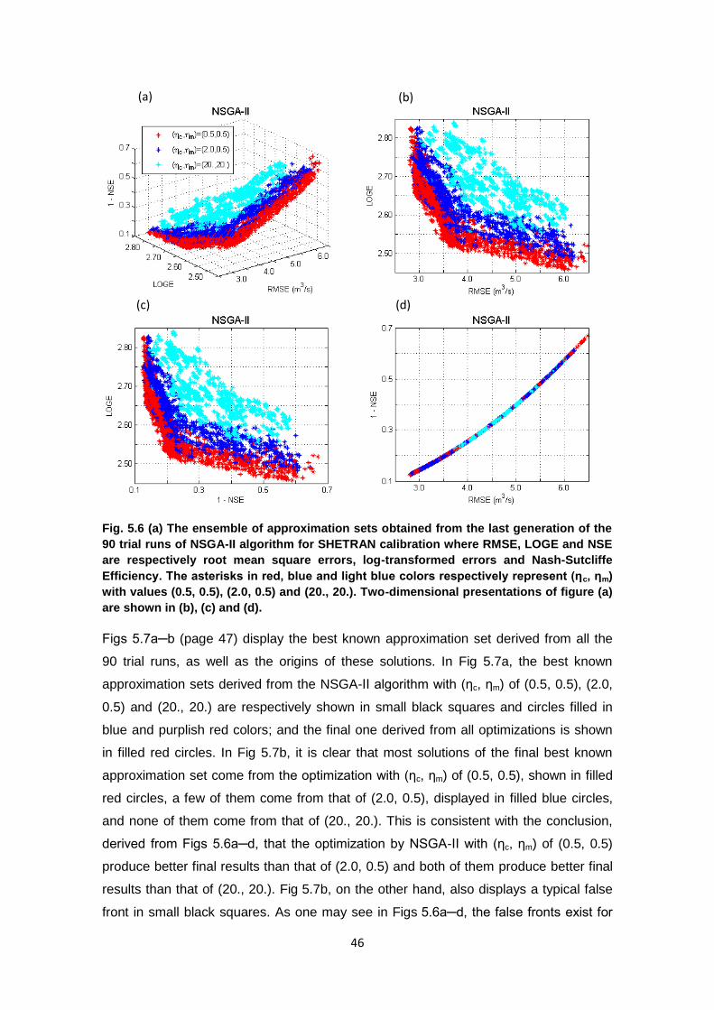
46
Fig. 5.6 (a) The ensemble of approximation sets obtained from the last generation of the
90 trial runs of NSGA-II algorithm for SHETRAN calibration where RMSE, LOGE and NSE
are respectively root mean square errors, log-transformed errors and Nash-Sutcliffe
Efficiency. The asterisks in red, blue and light blue colors respectively represent (ηc, ηm)
with values (0.5, 0.5), (2.0, 0.5) and (20., 20.). Two-dimensional presentations of figure (a)
are shown in (b), (c) and (d).
Figs 5.7a─b (page 47) display the best known approximation set derived from all the
90 trial runs, as well as the origins of these solutions. In Fig 5.7a, the best known
approximation sets derived from the NSGA-II algorithm with (ηc, ηm) of (0.5, 0.5), (2.0,
0.5) and (20., 20.) are respectively shown in small black squares and circles filled in
blue and purplish red colors; and the final one derived from all optimizations is shown
in filled red circles. In Fig 5.7b, it is clear that most solutions of the final best known
approximation set come from the optimization with (ηc, ηm) of (0.5, 0.5), shown in filled
red circles, a few of them come from that of (2.0, 0.5), displayed in filled blue circles,
and none of them come from that of (20., 20.). This is consistent with the conclusion,
derived from Figs 5.6a─d, that the optimization by NSGA-II with (ηc, ηm) of (0.5, 0.5)
produce better final results than that of (2.0, 0.5) and both of them produce better final
results than that of (20., 20.). Fig 5.7b, on the other hand, also displays a typical false
front in small black squares. As one may see in Figs 5.6a─d, the false fronts exist for
(a) (b)
(c) (d)

47
all the three optimizations, which have prevented them from reaching the best known
front. This phenomenon has been recognized by Tang et al. (2006) for multi-objective
calibration of the Leaf River SAC-SMA test by using the Ԑ-NSGA-II, SPEA2 and
MOSCEM-UA algorithms; this study displays the variability of the three optimizations’
performances of NSGA-II algorithm in Figs 5.8a─l (page 48) and Figs 5.9a─d (page
49).
Fig. 5.7 (a) The best known approximation sets derived from 30 trial runs of NSGA-II
algorithm with (ηc, ηm) of (0.5, 0.5), (2.0, 0.5) and (20., 20.) are respectively shown in small
black squares, filled blue circles and filled purplish red circles. The final one derived
from all trial runs is shown in filled red circles. (b) The final best known approximation
set is made up of solutions from trial runs of NSGA-II algorithm with (ηc, ηm) of (0.5, 0.5)
and (2.0, 0.5), respectively showing in filled red and blue circles. The false front, in small
black squares, is an example of the approximation set derived from a trapped trial run of
the NSGA-II algorithm.
Figs 5.8a─l (page 48) have shown the means and standard deviations of performance
metrics of NSGA-II with (ηc, ηm) of (0.5, 0.5), (2.0, 0.5) and (20., 20.) respectively in the
left, middle and right columns of plots; the means, standard deviations and variabilities
in performance are respectively shown in solid line, dash line and shaded area. From
the comparison of mean performances, it is clear that, for all the evolution processes,
the optimization by NSGA-II with (ηc, ηm) of (0.5, 0.5) produce better results than that of
(2.0, 0.5) and both of them lead to better final results than that of (20., 20.). To display
the significance of differences, for performances obtained by optimizations, the
Wilcoxon rank sum test was applied and the results show that performance metric
scores for all the three optimizations, are all significantly different from each other at
the 95% confidence level. From the comparison of the shaded areas, it is also shown
that there is large variability in performance, during all the 30 generations’ evolution
processes, for all the three optimizations; and the variability for NSGA-II with (ηc, ηm) of
(20., 20.) is always larger than the other two optimizations.
3.0 4.0 5.0 6.0
2.50
2.60
2.70
2.80
RMSE (m3/s)
LO
GE
(c,
m)=(0.5,0.5)
(c,
m)=(2.0,0.5)
False Front
3.0 4.0 5.0 6.0
2.50
2.60
2.70
2.80
RMSE (m3/s)
LO
GE
Final
(c,
m)=(0.5,0.5)
(c,
m)=(2.0,0.5)
(c,
m)=(20.,20.)
(a) (b)

48
Fig. 5.8 Plots of dynamic performance results of NSGA-II algorithm, namely hypervolume
(a, b and c), Ԑ-indicator (d, e and f), generational distance (g, h and i) and opt-indicator (j,
k and l), versus total number of SHETRAN model runs. Mean performance is indicated by
a solid line, the standard deviation by a dashed line, and the range of performance by the
shaded region. The left, middle and right columns of plots were respectively generated
from 30 trial runs of NSGA-II with (ηc, ηm) of (0.5, 0.5), (2.0, 0.5) and (20., 20.).
Figs5.9a─d (page 49) have shown the 50th and 95th percentiles of performance metrics
of NSGA-II with (ηc, ηm) of (0.5, 0.5), (2.0, 0.5) and (20., 20.) respectively in red, blue
and light blue colours; the 50th and 95th percentiles of performances are respectively
shown in dashed and bold solid lines and Figs 5.9a─d compare performances
respectively for hypervolume, Ԑ-indicator, generational distance and Opt-indicator. In
agreement with results shown in Figs 5.6a─d (page 46) and Figs 5.8a─l, for both 50th
and 95th percentiles of all four performance metrics and for nearly all the evolution
processes, the optimization by NSGA-II with (ηc, ηm) of (0.5, 0.5) produces better
0 5 10 150.0
0.3
0.6
0.9
Runs ( X 100)
Hyperv
olu
me
(a) (c,
m)=(0.5,0.5)
0 5 10 150.0
0.3
0.6
0.9
Runs ( X 100)
Hyperv
olu
me
(b) (c,
m)=(2.0,0.5)
0 5 10 150.0
0.3
0.6
0.9
Runs ( X 100)
Hyperv
olu
me
(c) (c,
m)=(20.,20.)
0 5 10 150.0
0.3
0.6
0.9
Runs ( X 100)
-In
dic
ato
r
(d) (c,
m)=(0.5,0.5)
0 5 10 150.0
0.3
0.6
0.9
Runs ( X 100)
-In
dic
ato
r
(e) (c,
m)=(2.0,0.5)
0 5 10 150.0
0.3
0.6
0.9
Runs ( X 100)
-In
dic
ato
r
(f ) (c,
m)=(20.,20.)
0 5 10 150.0
0.3
0.6
0.9
Runs ( X 100)
Genera
tional dis
tance
(g) (c,
m)=(0.5,0.5)
0 5 10 150.0
0.3
0.6
0.9
Runs ( X 100)
Genera
tional dis
tance
(h) (c,
m)=(2.0,0.5)
0 5 10 150.0
0.3
0.6
0.9
Runs ( X 100)G
enera
tional dis
tance
(i) (c,
m)=(20.,20.)
0 5 10 150.0
0.3
0.6
0.9
Runs ( X 100)
Opt-
Indic
ato
r
(j) (c,
m)=(0.5,0.5)
0 5 10 150.0
0.3
0.6
0.9
Runs ( X 100)
Opt-
Indic
ato
r
(k) (c,
m)=(2.0,0.5)
0 5 10 150.0
0.3
0.6
0.9
Runs ( X 100)
Opt-
Indic
ato
r
(l) (c,
m)=(20.,20.)

49
results than that of (2.0, 0.5) and both of them lead to better final results than that of
(20., 20.). This supports our proposal of using NSGA-II algorithm with (ηc, ηm) of (0.5,
0.5) for multi-objective automatic calibration of SHETRAN model for Cobres basin.
Fig. 5.9 Plots of dynamic performance results of NSGA-II algorithm, namely hypervolume
(a), Ԑ-indicator (b), generational distance (c) and opt-indicator (d), versus total number of
SHETRAN evaluations. The 50th
and 95th
percentiles of performance are respectively
indicated in dash and bold solid lines. The red, blue and light blue lines were respectively
generated from 30 trial runs of NSGA-II with (ηc, ηm) of (0.5, 0.5), (2.0, 0.5) and (20., 20.).
Validation of the best known approximation sets from the three optimizations
SHETRAN validation has been carried out for all the solutions of the best known
approximation sets derived from NSGA-II with (ηc, ηm) of (0.5, 0.5), (2.0, 0.5) and (20.,
20.). To make this a strong validation, results from the internal gauging stations
Albernoa and Entradas have also been evaluated. Figs 5.10a─l (page 50) display
SHETRAN model performance indicators, namely RMSE, LOGE and NSE, at basin
outlet Monte da Ponte and internal gauging stations Albernoa and Entradas
respectively in the left, middle and right columns of plots; results for the calibration
0 5 10 150.0
0.3
0.6
0.9
SHETRAN evaluations ( X 100)
Hyperv
olu
me
(a)
95% (c,
m)=(0.5,0.5) 95% (
c,
m)=(2.0,0.5) 95% (
c,
m)=(20.,20.)
0 5 10 150.0
0.3
0.6
0.9
SHETRAN evaluations ( X 100)
-In
dic
ato
r
(b)
50% (c,
m)=(0.5,0.5) 50% (
c,
m)=(2.0,0.5) 50% (
c,
m)=(20.,20.)
0 5 10 150.0
0.3
0.6
0.9
SHETRAN evaluations ( X 100)
Genera
tional d
ista
nce
(c)
0 5 10 150.0
0.3
0.6
0.9
SHETRAN evaluations ( X 100)
Opt-
Indic
ato
r
(d)

50
period are shown in the first two rows of plots and those for the validation period are
shown in the last two rows of plots; the filled red triangles, blue squares and black
circles respectively represent the solutions of the best known approximation sets
derived from optimizations by NSGA-II with (ηc, ηm) of (0.5, 0.5), (2.0, 0.5) and (20.,
20.).
Fig. 5.10 Plots of SHETRAN model performance indicators, namely RMSE, LOGE and
NSE, at basin outlet Monte da Ponte (a, d, g and j) and internal gauging stations Albernoa
(b, e, h and k) and Entradas (c, f, i and l). The results for the calibration period are
denoted by “(calib)” and those for the validation period by “(valid)”. The filled red
triangles, blue squares and black circles respectively represent the solutions of best
known approximation sets derived from 30 trial runs of NSGA-II with (ηc, ηm) of (0.5, 0.5),
(2.0, 0.5) and (20., 20.).
3.0 4.0 5.0 6.0
2.50
2.60
2.70
2.80
RMSE (m3/s)
LO
GE
(a) Monte da Ponte (calib)
(c,
m)=(0.5,0.5) (
c,
m)=(2.0,0.5) (
c,
m)=(20.,20.)
0.7 0.9 1.0 1.3 1.5
2.40
2.50
2.60
2.70
RMSE (m3/s)
LO
GE
(b) Albernoa (calib)
0.10 0.15 0.20
2.50
2.60
2.70
2.80
2.90
RMSE (m3/s)
LO
GE
(c) Entradas (calib)
0.1 0.3 0.5 0.7 0.9
2.50
2.60
2.70
2.80
NSE
LO
GE
(d) Monte da Ponte (calib)
0.1 0.3 0.5 0.7 0.9
2.40
2.50
2.60
2.70
NSE
LO
GE
(e) Albernoa (calib)
0.1 0.3 0.5 0.7 0.9
2.50
2.60
2.70
2.80
2.90
NSE
LO
GE
(f) Entradas (calib)
4.0 5.0 6.0 7.0 8.0
2.50
2.60
2.70
2.80
RMSE (m3/s)
LO
GE
(g) Monte da Ponte (valid)
1.1 1.3 1.5 1.7 1.9
2.80
2.90
3.00
RMSE (m3/s)
LO
GE
(h) Albernoa (valid)
0.50 0.60 0.70 0.80
2.30
2.40
2.50
2.60
2.70
RMSE (m3/s)
LO
GE
(i) Entradas (valid)
0.1 0.3 0.5 0.7 0.9
2.50
2.60
2.70
2.80
NSE
LO
GE
(j) Monte da Ponte (valid)
0.1 0.3 0.5 0.7 0.9
2.80
2.90
3.00
NSE
LO
GE
(k) Albernoa (valid)
0.1 0.3 0.5 0.7 0.9
2.30
2.40
2.50
2.60
2.70
NSE
LO
GE
(l) Entradas (valid)

51
For both the calibration (Figs 5.10a─f) and validation (Figs 5.10g─l) periods, it is shown
that the non-dominated solutions of the best known approximation set derived from
NSGA-II with (ηc, ηm) of (0.5, 0.5) dominate those from NSGA-II with (ηc, ηm) of (2.0, 0.5)
and (20., 20.) not only at basin outlet but also at internal gauging stations. The
dominance of the results from the optimization with (ηc, ηm) of (0.5, 0.5) is small relative
to those with (ηc, ηm) of (2.0, 0.5), as their non-dominated fronts overlap or locate near
each other, especially for the validation period; however, the dominance of results from
both optimizations with (ηc, ηm) of (0.5, 0.5) and (2.0, 0.5) are large compared to those
from optimization with (ηc, ηm) of (20., 20.), especially at basin outlet for the validation
period.
The results are very satisfactory in terms of NSE, as for the best simulation, the NSE,
for basin outlet, is 0.87 for calibration and 0.81 for validation; the NSE, for internal
gauging stations Albernoa and Entradas, is respectively 0.70 and 0.82 for calibration,
and 0.72 and 0.66 for validation. The Section 5.5.2 has shown that the study period
mainly consists of two main runoff generation periods, namely November 2005 and
October to December 2008, which are respectively preceded by 12 and 6 months’
droughts. Therefore, Figs 5.11a─d (page 52) have been made to display SHETRAN’s
capacity in reproducing storm events preceded by long periods of drought. Storms
No.1 and No.4 are the largest storm events respectively during the calibration and
validation periods. Figs 5.11a─b compare observed and simulated hydrographs for
storms No.1 and No.4 at basin outlet; Figs 5.11c─d compare observed and simulated
hydrographs for storm No.4 respectively at internal gauging stations Albernoa and
Entradas. The observed discharges are denoted as “Qobs” and shown in black line with
dots. The simulated discharges, denoted as “Qsim1”, “Qsim2”, “Qsim3” and “Qsim4” and
respectively shown in red, blue, purplish red, light blue lines, are from solutions with
respective objective functions (RMSE, LOGE, NSE), for basin outlet, of (2.81, 2.74,
0.87), (3.81, 2.53, 0.77), (4.85, 2.49, 0.63) and (5.85, 2.46, 0.46) for the calibration
period. The “Qsim1” simulation is the best solution, in terms of NSE or RMSE, from the
best known approximation set derived from the optimization by NSGA-II with (ηc, ηm) of
(0.5, 0.5). The NSE of “Qsim1”, for basin outlet, is 0.89 and 0.75 respectively for Storm
No.1 and No.4; for Albernoa and Entradas, they are respectively 0.74 and 0.66 for
Storm No.4. It is shown that the “Qsim1” reproduced very well the qualitative evolutions
of hydrographs at basin outlet, especially for Storm No.1, as well as at the two internal
gauging stations; however, it greatly underestimated the peak discharges, especially
for Storm No.4, and the simulated hydrographs are much less flashy than the observed
ones. As shown in Figs 5.11a─d, the other three simulations are solutions with larger

52
calibrated RMSEs (or smaller NSE), and their capacities of catching the storm peaks
are much smaller than “Qsim1”. In a sense, Figs 5.11a─d give a graphical impression on
the range of SHETRAN performances for storm events associated with the ranges of
RMSE or NSE for model calibration.
Fig. 5.11 Comparison between observed and simulated discharges from solutions
obtained from automatic calibration of SHETRAN model by NSGA-II algorithm: (a) Storm
No.1 at basin outlet; (b) Storm No.4 at basin outlet; (c) Storm No.4 at internal gauging
station Albernoa; (d) Storm No.4 at internal gauging station Entradas. “Qsim1”, “Qsim2”,
“Qsim3” and “Qsim4” are SHETRAN simulations, for the calibration period (2004-2006), with
objective functions (RMSE, LOGE, NSE) at basin outlet of respective values (2.81, 2.74,
0.87), (3.81, 2.53, 0.77), (4.85, 2.49, 0.63) and (5.85, 2.46, 0.46).
Conclusions
Multi-objective calibration of SHETRAN model has been carried out successfully to the
semi-arid Cobres basin with spatial resolution of 2.0 km and temporal resolution of 1 h
by using the NSGA-II algorithm. The SBX and PM were used as GA operators and
three optimizations were configured with (ηc, ηm) values of (0.5, 0.5), (2.0, 0.5) and (20.,
20.). The optimizations intend to simultaneously minimizing RMSE, LOGE and (1-NSE).
Each of them was repeated 30 times with initial parameter settings generated by the

53
LHS to eliminate the “random seed effects”. The results have shown that, as expected,
the RMSE function evolves in the same direction as (1-NSE) with the change of
proximity between observations and simulations. The calibration problem is actually a
two-objective optimization. By comparing the three optimizations, it is shown that the
one by NSGA-II with (ηc, ηm) of (0.5, 0.5) is the most efficient and achieved the best
final non-dominated set, and the one by NSGA-II with (ηc, ηm) of (20., 20.) is the least
efficient and achieved the worst final non-dominated set. This conclusion was made
from the comparison of all results, the mean performance and the 50th and 95th
percentile performances of the 30 trial runs among the three optimizations, as well as
the SHETRAN performances at basin outlet and internal gauging stations Albernoa and
Entradas, for solutions of the best known approximation sets, derived from the three
optimizations during both calibration and validation periods. Based on this, we
recommend values of the (ηc, ηm) of (0.5, 0.5), for NSGA-II in multi-objective calibration
of SHETRAN model, in basins with similar characteristics of climate, soil, land use and
topography. However, we cannot give a general conclusion on the use of smaller ηc
and ηm for accelerating the NSGA-II in multi-objective calibration of hydrological models,
as our study has used limited sets of ηc and ηm, our problem of optimization being a
very specific case.
5.6.4 NSGA-II Calibration of SHETRAN Sediment Parameters
Set-up of SHETRAN sediment parameters
The sediment parameters’ set-up is based on the results of hydrological parameters
calibration by using the MSCE scenario IV. It starts from the setting of vegetation
parameters shown in Table 5.5 (page 54), based on Wicks (1988), Lukey et al. (2000)
and a field survey of vegetation with similar climate condition. Then, soil particle size
distributions are estimated. Since there is no measurement available, the method of
Fooladmand and Sepaskhah (2006) is adopted to derive sediment particle-size
distribution from soil textural data. There are nine types of soil identified in SHETRAN
simulations with spatial resolution of 2.0 km for Cobres basin. Table 5.6 (page 54) has
shown their soil textural data extracted from Cardoso (1965). As shown, each type of
soil has one or two samples, and each sample has one to three horizons. Table 5.7
(page 55) has shown the sediment particle-size distribution, calculated by the method
of Fooladmand and Sepaskhah (2006), for all horizons of the soil samples. For each
soil type, the mass fraction of each sediment size group is an average, weighted by soil
depth, of the corresponding mass fractions from all the soil horizons and the final
results are displayed in Table 5.8 (page 55). Fooladmand and Sepaskhah (2006) have

54
indicated that their method is preferably applicable to soils with texture of silt content
less than 60% and particles with diameter larger than 0.05 mm. As shown in Table 5.6,
all soil types in Cobres basin are with texture of silt less than 60%. Since the particle
diameters for which the mass fractions are calculated are all larger than 0.05 mm, the
applicability of Fooladmand and Sepaskhah (2006) to our study is justified.
Table 5.5 Vegetation parameters for sediment transport simulations of Cobres basin
Parameter Crop Agroforestry Forest Bush
Percentage of canopy drainage falling as drips (%) 80 80 80 80
Drip diameter from canopy (mm) 5 5 5 5
Average drip fall height from canopy (m) 0.8 3.0 3.0 1.0
Percentage canopy cover (Cc) (%) 90 50 90 90
Percentage ground cover (Cg) (%) 90 50 90 90
Table 5.6 Soil textural data from Cardoso (1965) for soil types in Cobres basin
Soil type
Soil sample
Sample number
Horizon Soil depth
(m) Sand (%)
Silt (%)
Clay (%)
Vx
Vx-459 9382 A1 0.15 33.5 39.4 27.1
9383 B2 0.35 10.4 34.4 55.2
Vx-460 9385 Ap 0.18 28.7 41.0 30.3
9386 B2 0.47 27.8 30.6 41.6
Px
Px-455 9369 Ap 0.20 61.6 22.1 16.3
9370 B2 0.20 54.9 20.2 24.9
Px-457 9375 A1 0.15 47.3 36.0 16.7
9376 B2 0.20 35.9 37.6 26.5
Ex Ex-140 8500 Ap 0.10 50.2 24.2 25.6
Ex-144 8505 Ap 0.10 82.9 11.0 6.1
Bvc
Bvc-202 4687 Ap 0.25 23.9 22.2 53.9
4688 B 0.15 21.3 20.1 58.6
Bvc-204 5884 Ap 0.30 15.6 23.7 60.7
5885 B 0.50 15.4 24.8 59.8
Cb
Cb-10
7420 Ap 0.20 70.2 10.2 19.6
7421 A3 0.20 68.0 10.2 21.8
7422 B 0.20 65.5 10.3 24.2
Cb-334
8372 Ap 0.32 58.9 12.5 28.6
8373 B2 0.28 45.0 12.1 42.9
8374 B3 0.18 51.8 16.6 31.6
Ppm Consider it as the same as Cb soil
Sr
Sr*-229
8188 Ap 0.25 66.6 15.7 17.7
8189 A3 0.28 59.7 16.0 24.3
8190 B2 0.22 53.4 11.0 35.6
Sr*-4 9401 Ap 0.20 77.7 13.1 9.2
9402 B 0.15 71.5 16.0 12.5
Ppg Ppg-62 8318 Ap 0.20 74.8 13.1 12.1
8319 B 0.30 71.6 14.2 14.2
Ep Ep-148 8513 Ap 0.10 71.0 16.9 12.1

55
Table 5.7 Soil particle-size distribution for soil types in Cobres basin
Soil type
Soil sample
Sample number
Horizon
Mass fraction of sediment size groups (%)
0.10 (mm)
0.37 (mm)
0.89 (mm)
1.59 (mm)
2.00 (mm)
Vx
Vx-459 9382 A1 78.9 17.2 3.4 0.5 0.0
9383 B2 94.3 4.8 0.8 0.1 0.0
Vx-460 9385 Ap 82.5 14.4 2.7 0.4 0.0
9386 B2 82.0 14.4 3.2 0.4 0.0
Px
Px-455 9369 Ap 52.2 35.1 11.2 1.4 0.1
9370 B2 57.2 30.8 10.5 1.4 0.1
Px-457 9375 A1 68.2 25.5 5.5 0.7 0.1
9376 B2 76.9 18.7 3.8 0.5 0.1
Ex Ex-140 8500 Ap 62.6 28.0 8.2 1.1 0.1
Ex-144 8505 Ap 27.0 45.8 24.1 2.9 0.2
Bvc
Bvc-202 4687 Ap 83.9 12.6 3.0 0.4 0.1
4688 B 85.7 11.1 2.7 0.4 0.1
Bvc-204 5884 Ap 90.4 7.8 1.6 0.2 0.0
5885 B 90.6 7.6 1.6 0.2 0.0
Cb
Cb-10
7420 Ap 38.4 36.2 22.1 3.1 0.2
7421 A3 40.6 35.1 21.1 3.0 0.2
7422 B 43.0 33.9 20.0 2.9 0.2
Cb-334
8372 Ap 50.4 31.7 15.5 2.2 0.2
8373 B2 63.3 24.3 10.7 1.6 0.1
8374 B3 58.7 28.7 11.0 1.5 0.1
Ppm Consider it as the same as Cb soil
Sr
Sr*-229
8188 Ap 44.8 37.2 15.8 2.0 0.2
8189 A3 51.3 33.1 13.7 1.8 0.1
8190 B2 55.0 28.3 14.4 2.1 0.2
Sr*-4 9401 Ap 33.2 43.4 20.7 2.5 0.2
9402 B 40.5 40.5 16.7 2.1 0.2
Ppg Ppg-62 8318 Ap 35.8 41.2 20.2 2.6 0.2
8319 B 39.4 39.7 18.4 2.3 0.2
Ep Ep-148 8513 Ap 41.4 40.5 15.9 2.0 0.2
Table 5.8 Mass fraction for sediment particle-size distribution of soil types in Cobres basin
Particle diameter
(mm) 0.10 0.37 0.89 1.59 2.00
Mass
Fraction
(%)
Vx 85.4 11.8 2.4 0.3 0.1
Px 63.3 27.7 7.9 1.0 0.1
Ex 44.8 36.9 16.1 2.0 0.2
Bvc 88.5 9.2 2.0 0.3 0.0
Cb 49.9 31.3 16.3 2.3 0.2
Ppm 49.9 31.3 16.3 2.3 0.2
Sr 45.8 35.9 16.0 2.1 0.2
Ppg 37.9 40.3 19.1 2.5 0.2
Ep 41.4 40.5 15.9 2.0 0.2

56
Then, the overland flow sediment transport capacity equation is selected, based on the
results of simulations shown in Table 5.9 (page 57). Considering the possible variations
of rainfall impact erodibility and overland flow erodibility, the simulated suspended
sediment yield would be in the range of [0.029, 0.062] t/ha/year by using the Engelund-
Hansen equation; and it would be in the range of [0.052, 14.732] t/ha/year by using the
Yalin equation. The use of Yalin equation may provide a reasonable range of sediment
yields, taking the basin size and the literature studies into consideration. According to
Walling (1983), the observed sediment yields for catchments of around 1000 km2 are in
the range of [0.1, 10.0] t/ha/year. Bathurst et al. (1996) observed the sediment yields,
for the 167-m2 soil erosion plots at the Centro Experimental de Erosão de Vale
Formoso, just to the east of the Cobres basin, in the ranges of [0.44, 2.0], [1.10, 1.34]
and [0.24, 1.10] t/ha/year for the respective Wet (1977─1979), Dry (1980─1982) and
Mean (1983─1985) periods. Since Cobres basin is of area 705 km2, it is most probable
that the sediment yield with values larger than 0.1 t/ha/year. Consequently, this
excludes the eligibility of the Engelund-Hansen equation for the simulation of overland
flow sediment transport capacity. As for the channel flow sediment transport capacity,
three equations are available: the Engelund-Hansen equation, the Acker-White
equation and the Ackers-White-Day equation. Experiments, not shown in thesis, have
indicated that the sediment yield varies very little with the selection of different equation,
so the Engelund-Hansen equation is used.

57
Tab
le 5
.9 P
reli
min
ary
sed
imen
t sim
ula
tio
ns o
f C
ob
res b
asin
fo
r th
e p
eri
od
fro
m O
cto
ber,
2004
to
No
vem
ber,
200
6
Mo
del
ru
na
k r
(J-1
) k f
(m
g m
-2 s
-1)
k b
(mg
m-2
s-1
) IS
GSE
D
ISA
CK
W
FPC
RIT
(%
) D
LSM
AX
(m
m)
DC
BED
O
(mm
) D
LS
(mm
) Fi
ne
sed
yie
ld
t h
a-1·y
ear-1
To
tal s
ed y
ield
t
ha-1
·yea
r-1
No
.1
0.0
1
0.0
1
0.0
1
0
2
5
50
1
0
0.0
0
.02
86
0
.04
14
No
.2
0.0
1
0.1
0
.0
1
0
25
5
0
10
0
.0
0.0
59
4
0.0
82
7
No
.3
0.0
5
0.1
0
.0
1
0
25
5
0
10
0
.0
0.0
59
6
0.0
82
9
No
.4
0.1
0
.1
0.0
1
0
2
5
50
1
0
0.0
0
.05
97
0
.08
31
No
.5
1.0
1
.0
0.0
1
0
2
5
50
1
0
0.0
0
.06
19
0
.08
57
No
.7
2.0
2
.0
0.0
1
0
2
5
50
1
0
0.0
0
.06
19
0
.08
57
No
.6
2.0
2
0.0
0
.0
1
0
25
5
0
10
0
.0
0.0
61
9
0.0
85
7
No
.8
10
.0
20
.0
0.0
1
0
2
5
50
1
0
0.0
0
.06
19
0
.08
57
No
.9
0.0
1
0.0
1
0.0
0
0
2
5
50
1
0
0.0
0
.05
17
0
.07
18
No
.10
0
.01
0
.05
0
.0
0
0
25
5
0
10
0
.0
0.2
47
6
0.3
02
3
No
.11
0
.1
0.1
0
.0
0
0
25
5
0
10
0
.0
0.4
93
4
0.5
64
5
No
.12
0
.1
0.5
0
.0
0
0
25
5
0
10
0
.0
2.1
69
3
2.2
88
2
No
.13
1
.0
1.0
0
.0
0
0
25
5
0
10
0
.0
4.1
13
8
4.2
50
1
No
.14
2
.0
2.0
0
.0
0
0
25
5
0
10
0
.0
7.1
87
3
7.3
30
4
No
.15
2
.0
20
.0
0.0
0
0
2
5
50
1
0
0.0
1
4.6
85
6
14
.83
18
No
.16
1
0.0
2
0.0
0
.0
0
0
25
5
0
10
0
.0
14
.73
23
1
4.8
78
4
No
te:
a k r a
nd
kf a
re r
esp
ecti
vely
rai
nd
rop
imp
act
ero
dib
ility
an
d o
verl
and
flo
w e
rod
ibili
ty, k
b is
ban
k fl
ow
ero
dib
ility
. ISG
SED
wit
h v
alu
e o
f 1
(0
) m
ean
s th
e En
gelu
nd
-Han
sen
(Ya
lin)
equ
atio
n i
s se
lect
ed f
or
calc
ula
tio
n o
f o
verl
and
flo
w s
edim
ent
tran
spo
rt c
apac
ity.
ISA
CK
W w
ith
val
ue
of
0 m
ean
s En
gelu
nd
-Han
sen
eq
uat
ion
is
sele
cted
fo
r ca
lcu
lati
on
of
chan
nel
flo
w s
edim
ent
tran
spo
rt c
apac
ity.
FP
CR
IT is
use
r sp
ecif
ied
max
imu
m s
edim
ent
con
cen
trat
ion
th
at c
an b
e ca
rrie
d b
y fl
ow
, an
d 2
5 %
is s
et t
o p
relim
inar
y si
mu
lati
on
s
wh
ich
is e
qu
ival
ent
to 6
62
.5 g
/l.
DLS
MA
X w
ith
val
ue
of
50
mm
mea
ns
that
if t
he
dep
th o
f lo
ose
sed
imen
t th
at b
uild
s u
p o
n t
he
hill
slo
pe
reac
hes
50
mm
, th
e so
il u
nd
ern
eath
is a
ssu
med
to
be
pro
tect
ed a
nd
no
fu
rth
er e
rosi
on
tak
e p
lace
. D
CB
EDO
wit
h v
alu
e o
f 1
0m
m m
ean
s th
at t
he
dep
th o
f ac
tive
to
p b
ed
laye
r is
set
to
10
mm
. Fi
ne
sed
imen
t is
con
sid
ered
as
sed
imen
t w
ith
dia
met
er le
ss t
han
0.1
mm
.

58
Previous studies by Wicks et al. (1992), Wicks and Bathurst (1996), Adams and Elliott
(2006), and Bathurst (2011) have indicated that the soil erodibility coefficients increase
in value as the soil becomes easier to erode. The raindrop impact and overland flow
erodibility coefficients are not directly measurable soil properties and are therefore
required to be adjusted in calibration process according to model grid square scale, soil
texture, soil conditions such as moisture content, animal effects such as compaction by
grazing cattle, human effects such as tillage, and vegetation effects such as root
binding. Bathurst et al. (1996) found the erodibility coefficients need to be varied
between moderate rainfall events and extreme events. As for sediment transport
simulations at Cobres basin, they used a ‘normal’ set (kr = 0.13 J-1, kf = 1.3 mg/m2/s)
calibrated on all events other than the extreme event; and an ‘extreme’ set (kr = 2.0 J-1,
kf = 20.0 mg/m2/s) calibrated on the largest erosion event in the calibration period. In
this study, the simulation period is even drier than the dry period of Bathurst et al.
(1996), as one may see in Table 5.10. Therefore, the erodibility coefficients may be
smaller than the ‘normal’ set given by Bathurst et al. (1996), since in dry condition the
surface soils are harder and less erodible than those in wetter conditions as explained
in Adams and Elliott (2006). Preliminary simulations No.9 to No.13, shown in Table 5.9
(page 57), have indicated that simulated sediment yields could be in the range of
[0.052, 4.114] t/ha/year, which is in agreement with those derived from the plot
measurement of Bathurst et al. (1996), if the ranges of rainfall impact erodibility and
overland flow erodibility coefficients are respectively set as [0.01, 1.0] J-1 and [0.01, 1.0]
mg/m2/s. Thus, for sediment parameter calibration, the range of raindrop impact
erodibility and overland flow erodibility are respectively set as [0.01, 1.0] J-1 and [0.01,
1.0] mg/m2/s. For baseline simulations, the raindrop impact erodibility is set as 0.1, 0.2
and 1.0 J-1 and the overland flow erodibility is set as 0.05, 0.1 and 0.5 mg/m2/s
respectively for clay, loam and Sandy loam.
Table 5.10 Statistics of annual rainfall and runoff at Cobres basin
Description Yeara
Rainfall (mm)
Runoff (mm)
Dry period in Bathurst et al. (1996)
b
1980─1981 250 0
1981─1982 483 86
Calibration simulation period in Rong et al. (2013)
c
2004─2005 194 0
2005─2006 502 55
Note: aYears are defined October to September.
bData is extracted from Bathurst et al. (1996).
cData is extracted from Rong et al. (2013).

59
NSGA-II calibration of SHETRAN sediment parameters
The observed sediment discharge data for the period of Storm No.4, namely from
October 23rd, 2006 05:00 to October 27th, 2006 23:00, is used in the automatic
calibration of SHETRAN sediment parameters by NSGA-II algorithm with (ηc, ηm) of
(0.5, 0.5). In the calibration of sediment parameters, the NSGA-II was preferred to
MSCE since this last method is too time consuming. However, for the calibration of
hydrological parameters, we used the previously computed set obtained from MSCE.
Each SHETRAN simulation is carried out for the period from October 1st 2004 to
November 4th 2006, using the hydrological parameters calibrated by MSCE as
described in Section 5.5.2. The population size is set to 50; a maximum of 50
generations is prescribed for each trial run and only one trial run is performed. The
optimization produced a non-dominated set of solutions in terms of RMSE and LOGE,
from which the one with minimum RMSE was selected with the intention of getting
better performance for sediment transport simulation during high flow processes. The
calibrated (kr, kf), for the Vx, Px and Ex soils, are respectively (0.01 J-1, 0.01 mg/m2/s),
(0.01 J-1, 0.01 mg/m2/s) and (1.00 J-1, 0.58 mg/m2/s). The model performance
indicators, namely RMSE, LOGE and NSE, for comparison between observed and
simulated hourly sediment discharges are respectively 40.25 kg/s, 2.45 and 0.56.
Fig 5.12 (page 60) compares observed and simulated hourly discharges and sediment
discharges for Storm No.4. It can be seen that, for sediment discharge simulation,
SHETRAN model greatly underestimated the first peak and overestimated all the
recession process of the three peaks. After a long period of drought, the first peak of
Storm No.4 transported a large amount of sediment due to the abundant sediment
deposition, while the second and third peaks transported much less sediment than their
precedent peaks probably due to the lack of deposited sediment as well as the smaller
rainfall intensities as shown in Fig. 5.5b (page 40). And SHETRAN model did not
represent well this process. For Storm No.4, the simulation overestimated the observed
sediment yield (0.200 t/ha) by 78 %. Overall, the simulated sediment yield is 0.724
t/ha/year, which is in the range of [0.1, 10.0] t/ha/year, as suggested by Walling (1983).
The calibration is satisfactory considering the nature and quantity of the observed
sediment data.

60
Fig. 5.12 Comparisons between observed and simulated hourly discharges and sediment
discharges for the solution obtained from automatic calibration of sediment parameters
by NSGA-II. “Qobs”, “Qsim”, “Qsedobs” and “Qsedsim” respectively represent observed
discharge, simulated discharge, observed sediment discharge and simulated sediment
discharge. Time is shown in the “MM/DD/YY” format.
5.7 Discussion
Automatic calibration is preferred because it provides an objective and extensive
searching in the feasible parameter space. In this chapter, the applicability and
efficiency of the MSCE and NSGA-II algorithms have been demonstrated for automatic
calibration of SHETRAN model in the semi-arid Cobres basin with spatial resolution of
2.0 km and temporal resolution of 1 h. To simplify the process, we divided the
calibration parameters into hydrological parameters and sediment parameters. The
calibration started with the hydrological parameters and the results were used in
following calibration of sediment parameters. The entire calibration process can be
completed by either MSCE or NSGA-II independently. In this study, we calibrated the
hydrological parameters of SHETRAN model by MSCE with the objective of minimizing
RMSE; and then, using the obtained hydrological parameters, we calibrated the
sediment parameters by NSGA-II with the objective of minimizing RMSE and LOGE;
finally, the solution from the non-dominated set with minimum RMSE was selected.
For Cobres basin with spatial resolution of 2.0 km, twenty-two hydrological parameters
were identified to be calibrated considering the key parameters of the two main types of
10/21/06 10/23/06 10/25/06 10/27/06 10/29/060
100
200
300
400
Time (hour)
Qhrd
is (
m3/s
) NSEsim
=0.64
NSEsedsim
=0.56
0
100
200
300
400
Qhrs
eddis
(kg
/s)
Qobs
Qsim
Qsedobs
Qsedsim

61
land-use and the three main types of soil; and six sediment parameters were identified
for the main types of soil. The results are very satisfactory for both MSCE and NSGA-II
calibrations of hydrological processes. As for the MSCE (the best solution from NSGA-
II) calibration, NSE, for basin outlet, is 0.86 (0.87) for calibration and 0.74 (0.81) for
validation; NSE, for internal gauging stations Albernoa and Entradas, is respectively
0.65 (0.70) and 0.82 (0.82) for calibration, 0.69 (0.72) and 0.63 (0.66) for validation; as
for storm events, NSE, for basin outlet, is 0.87 (0.89) and 0.64 (0.75) respectively for
Storms No.1 (during the calibration period) and No.4 (during the validation period); for
Albernoa and Entradas, it is respectively 0.69 (0.74) and 0.65 (0.66) for Storm No.4.
For the MSCE and NSGA-II calibrations, trial runs of optimizations were performed
respectively once and ninety times, therefore no comparability exists between them.
For NSGA-II, the SBX and PM were used as GA operators. Three optimizations were
configured with (ηc, ηm) of respective values (0.5, 0.5), (2.0, 0.5) and (20., 20.); all of
them were repeated 30 times with initial parameters randomly generated by the LHS.
Comparisons have shown that the one with (ηc, ηm) of (0.5, 0.5) is the most efficient
and provides best final solutions. Thus, NSGA-II algorithm with (ηc, ηm) of (0.5, 0.5) is
recommended to multi-objective calibration of SHETRAN model in basins with similar
characteristics of climate, soil, land use and topography.
The sediment parameters were calibrated for Storm No.4 by NSGA-II algorithm with (ηc,
ηm) of (0.5, 0.5) and by using the hydrological parameters derived from the MSCE
calibration. The result is satisfactory considering the low quality of the observed
sediment data. For Storm No.4, the NSE, for basin outlet, is 0.56 for hourly sediment
discharges and the simulation overestimated the sediment yield by 78%. The simulated
sediment yield is 0.724 t/ha/year for the 25 months’ simulation period, which is in the
range, [0.1, 10.0] t/ha/year, given by Walling (1983). Therefore, the twenty-two
hydrological parameters calibrated by MSCE and the six sediment parameters
calibrated by NSGA-II are used in hydrological simulations of control and future climate
scenarios, in Chapter 8.

62

63
6. Impacts of Spatial Scale on the SHETRAN Model
The impacts of spatial scale on SHETRAN hydrological simulations are described in
this chapter. The objective of it is, based on the available data, to form a basis for the
selection of proper spatial resolution for the SHETRAN hydrological simulations, and
evaluating future climate change impacts. First, a concise introduction is presented;
then the methods and data are described; next, the impacts of spatial scale on long-
term runoff simulation and storm-runoff generation are respectively assessed; finally, a
short discussion concludes this chapter.
6.1 Introduction
Similarly to other PBSD models, the application of the SHETRAN model requires the
specification of spatial resolutions, both horizontally and vertically, for model
simulations. Usually, the selection of a proper spatial resolution is a compromise
among the availabilities of input data, such as DEM, maps of land-use and soil type,
computational resources and the modelling purposes (Ewen et al., 1996; Henriksen et
al., 2003). This is particularly true for basins with areas of middle to large sizes. The
use of coarse spatial discretization can simplify the model set-up and reduce the work
involved in data collecting and processing, as well as the execution time of model
simulation; however, it may also cause the loss or inaccurate representation of
information such as types of land-use and soil and drainage density, which would
ultimately decrease the model performance. It is therefore desirable to investigate the
effects of spatial resolution on model performance.
Previous studies about the effects of spatial discretization on model performance can
be found in Refsgaard (1997) and Vázquez et al. (2002) for the MIKE-SHE model and
Wildemeersch et al. (2014) for the HydroGeoSphere model. Their work leads to the
conclusion that coarse grids may result in a poor simulation of discharges, due to the
inadequate representation of the catchment river links. Although this conclusion was
based on simulations with different grid sizes, the corresponding calibrations were
either absent, or manual, or partially objective. In the present research, a fully objective
global optimization method is used to compare the results from the simulations
proposed for different horizontal spatial resolutions. The conclusion will be used,
together with other information, in determining the final selection of an appropriate
horizontal spatial resolution for SHETRAN simulations at Cobres basin, aiming to
evaluate future climate change impacts, as described in Chapter 8.

64
6.2 Methods and Data
Three important aspects are essential for comparing the impacts of spatial
discretization: (1) the possible model performances; (2) the final best model
performances as well as their parameter settings; (3) the best model performances
achieved by each step of the optimization process. They are designed to give an
overall evaluation of the fitness of a spatial resolution to the model simulations. NSGA-
II algorithm is a global optimization method which is capable of finding the non-
dominated optimal solutions through searching of the whole possible parameter setting
spaces (Deb et al., 2002). Therefore, aspect (1) can be evaluated by comparison of
ensembles of SHETRAN simulations from the whole set of optimization processes of
different spatial resolutions. To be specific, the best solutions from each optimization
step are included to form the ensemble of best solutions. Chapter 5 has demonstrated
that the NSGA-II algorithm, together with the SBX and PM genetic algorithm operators
and with (ηc, ηm) of (0.5, 0.5), is effective and efficient in SHETRAN model calibration.
So, aspect (3) can be assessed by comparison of the best solutions for each evolved
optimization step, and the selection of the final one, provides a conclusion for aspect
(2).
Considering the availability of computational resources, we propose the comparison of
spatial resolutions of 0.5, 1.0 and 2.0 km for the evaluation of spatial scale impacts on
model performance; and each of the single SHETRAN simulation requires respectively
around 45, 12 and 3 minutes. The NSGA-II parameters are set the same as described
in Chapter 5. The SHETRAN calibrations are configured to evolve 30 generations with
population size of 50 for minimizing the objective functions of RMSE, LOGE and (1-
NSE), for each spatial resolution, by using the NSGA-II algorithm with (ηc, ηm) of (0.5,
0.5). By simultaneously performing 4 simulations, the model calibrations demand
around 338, 64 and 16 hours to be completed respectively for spatial resolutions of 0.5,
1.0 and 2.0 km. Therefore, they will not be repeated to eliminate the random seed
effects; instead, an initial parameter setting LHS1, sampled by the LHS technique, is
used for the SHETRAN calibrations.
As in Chapter 5, the calibration period is set as from October 1st 2004 to September
30th 2006 and the objective functions are evaluated based on comparisons between
observed and simulated hourly discharges at basin outlet, Monte da Ponte gauging
station. For spatial resolution of 2.0 km, the SHETRAN model set-up and performance
can be found in detail respectively in Sections 5.3 and 5.6.3. For the spatial resolutions
of 0.5 and 1.0 km, the SHETRAN model is set up in the same way as described in

65
Section 5.3 and the twenty-two calibration parameters are constrained within the
physically realistic ranges listed in Table 5.2 (page 31). Moreover, SHETRAN is also
set up for the spatial resolution 1.5 km, but not calibrated due to computational limits;
and its maps of land-use, soil types and river links will be displayed together with those
from the other three spatial resolutions, to illustrate the effect of spatial resolutions on
the model input.
The best solutions from model calibration are selected based on the criterion of NSE ≥
0.85 and validated for the spatial resolutions of 1.0 and 2.0 km for possible future
applications. For validation, the 0.5 km resolution was not considered, as explained in
Section 6.4.1. According to Klemeš (1986), Bathurst et al. (2004) and Refsgaard et al.
(2014), the SHETRAN model is validated from these four aspects: (1) Split-sample test;
(2) Differential split-sample test; (3) Proxy-basin test and (4) Multi-site test, namely for
internal and outlet responses. Based on SHETRAN simulations at Cobres basin, the
validations (1) and (4) are carried out by comparing the observed and simulated hourly
discharges at basin outlet and internal gauging stations Albernoa and Entradas for the
period from October 1st 2006 to September 30th 2008; validation (2) is performed by
comparisons of hourly discharges at basin outlet for the period from October 1st 1977 to
September 29th 1979. Based on SHETRAN simulations at Albernoa basin, the
validations (3) and (4) are assessed by comparing the observed hourly discharges with
the simulations at basin outlet and internal gauging station Entradas for the periods
from October 1st 2004 to September 30th 2006 and from October 1st 2006 to September
30th 2008. As the validations involve solutions with equally or nearly equally good
model performances, the equifinality condition (Beven and Freer, 2001) can also be
identified and tested. The rainfall, PET and discharge data were provided by Professor
Bathurst, University of Newcastle, for the SHETRAN simulations at Cobres basin, for
the period from October 1st 1977 to September 29th 1979.
The SHETRAN model calibrations and validations are evaluated in terms of long-term
runoff and storm-runoff simulations. For long-term runoff simulation, the objective
functions RMSE, LOGE and NSE are evaluated as well as graphics of model fit and
monthly and annual mass balance errors. In order to validate the model’s capability of
reproducing extreme storm events, the events with peak discharges at Monte da Ponte
gauging station with values larger than 200 m3/s are selected for evaluation of storm-
runoff simulation, by comparisons of objective functions such as NSE, mass balance
error (MBE) and peak error (PKE), as well as, graphics of model fit. Definitions of MBE
and PKE are shown in equations 6.1 and 6.2.

66
n
i
i
n
i
ii
O
OS
MBE
1
1 6.1
pk
obs
pk
obs
pk
sim
Q
QQPKE
6.2
Where Oi and Si are respectively observed and simulated hourly discharges at ith hour;
n is the total number of hours; pk
obsQ and pk
simQ are respectively observed and simulated
peak discharges.
6.3 Impacts of Spatial Scale on the SHETRAN Model Input
Figs 6.1a–d (page 67), 6.2a–d (page 68) and 6.3a–d (page 69) respectively represent
the impacts of spatial scale on the maps of land-use, soil type and river links. Table 6.1
(page 69) indicates the impact of spatial scale on drainage density of the Cobres basin.
It is shown that the grid coarsening have caused (1) the loss of land-use and soil types,
(2) reduction of the drainage density and (3) the misrepresentation of the land-use, soil
type and river links. As shown in Figs 6.1a–d (page 67), the land-use type “urban” is
identified in spatial resolutions of 0.5 and 1.0 km but not in the resolutions of 1.5 and
2.0 km; the “bush” is scattered in both south and northeast of the basin for spatial
resolutions of 0.5 and 1.0 km, however, it is only concentrated in the south for the
resolutions of 1.5 and 2.0 km. Similar situations can be found for the soil types “Cb”,
“Ppm” and “Sr” in Figs 6.2a–d (page 68). Figs 6.3a–d (page 69) have demonstrated the
better representations of river links in SHETRAN simulations, shown in red lines, by
using the finer spatial resolutions. Notice that the “Cobres river INAG” was provided by
SNIRH based on the map with scale of 1:100000. Table 6.1 (page 69) indicates that
coarser resolution reduces the drainage density: the spatial resolution of 2.0 km
reduces by around 18% the drainage density of 0.5 km resolution.

67
Fig. 6.1 Maps of land-use distribution for Cobres basin with respective spatial resolutions
of 0.5, 1.0, 1.5 and 2.0 km.
(a)
(c) (d)
(b)

68
Fig. 6.2 Maps of soil type distribution for Cobres basin with respective spatial resolutions
of 0.5, 1.0, 1.5 and 2.0 km.
(a)
(c) (d)
(b)

69
Fig. 6.3 Maps of river links distribution for Cobres basin with respective spatial
resolutions of 0.5, 1.0, 1.5 and 2.0 km. The red lines represent river links, introduced by
the non-standard set-up, developed in the thesis, in the SHETRAN simulations, and the
purple ones indicate those provided by SNIRH.
Table 6.1 Area, total river length and drainage density of the Cobres basin
Spatial resolution 2.0 km 1.5 km 1.0 km 0.5 km DEM (10 m)
Basin area (km2) 700 713.25 705 664.5 705.3
Total river length (km) 262 274.5 294 304.5 694.7
Drainage density (km/km2) 0.374 0.385 0.420 0.458 0.985
(b) (a)
(c) (d)

70
6.4 Impacts of Spatial Scale on the SHETRAN Model Performance
6.4.1 Introduction
This section presents the impacts of spatial scale on the SHETRAN model
performance, in terms of long-term runoff simulation and storm-runoff generation, for
both the calibration and validation periods. For calibration, the spatial resolutions of 0.5,
1.0 and 2.0 km were considered for the simulation at Cobres basin and comparisons
were made for their model performances during the optimization processes (Figs 6.4–
6.6, pages 71–73). Based on the criterion of NSE ≥ 0.85, the 8 and 25 best solutions,
shown in Table 6.2 (pages 75–76), were respectively selected from the final results of
the SHETRAN calibrations, with the spatial resolutions of 1.0 and 2.0 km for model
validations, for possible future applications. For validation, the 0.5 km resolution was
not considered, taking into account serious computational limitations, and the fact that
validation was corroborated by higher than 0.85 Nash-Sutcliffe Efficiencies, for the two
not so optimal spatial resolutions. For both calibration and validation periods, the
selected best solutions were evaluated on long-term runoff simulation by using the
split-sample test, differential split-sample test, proxy-basin test and multi-site test; and
they were assessed on storm-runoff generation by considering the key factors
important for sediment transport simulation such as peak discharge, storm runoff and
storm hydrograph. The evaluations of long-term runoff simulations are shown in Figs
6.7a–l, 6.8a–b, 6.9a–h, 6.10a–h, 6.11a–c, 6.12a–c (pages 79–84) and Tables 6.3 and
6.4 (pages 81 and 83); the assessments of the storm-runoff generations are indicated
in Figs 6.13, 6.14a–b, 6.15a–d, 6.16a–d and 6.17a–e (pages 85–89).
6.4.2 Impacts of Spatial Scale on Long-Term Runoff Simulation
Model performances during the optimization processes
Figs 6.4a–c (page 71) compare model performances obtained from the entire
optimization processes of the different spatial resolutions based on the same initial
parameter setting LHS1.

71
Fig. 6.4 Plots showing the comparisons of SHETRAN performances resulting from
different spatial discretizations. The black (and light blue), blue and red asterisks
represent the ensembles of elite solutions derived from the processes of SHETRAN
calibration for Cobres basin with respective spatial resolutions of 2.0, 1.0 and 0.5 km. The
subscripts LHS1 and LHSall respectively represent the 1st
and all the 30 initial parameter
settings generated by the LHS technique. The NSGA-II algorithm with (ηc, ηm) of (0.5, 0.5)
was used for calibration.
Fig 6.4a displays the comparison of model performances with objectives RMSE, LOGE
and (1-NSE), and Figs 6.4b–c indicate comparisons in projections on 2-D spaces
RMSE.vs.LOGE and (1-NSE).vs.LOGE. It is clear that the model performances for
(a) (b)
(c) (d)
(e) (f)

72
different spatial resolutions are located in distinctly different regions of the objective
spaces. All in all, three conclusions can be taken: (1) all SHETRAN simulations for the
1.0 km resolution are better than those for the 2.0 km resolution and nearly all
simulations for the 0.5 km resolution are better than those for the 1.0 km resolution; (2)
Among all objectives, by using the finer spatial resolution, LOGE is improved to the
maximum extent and the improvement is for all the possible simulations; however the
RMSE and NSE are improved distinctly only for the best simulations. As indicated in
Figs 6.4b–c, from the 2.0 to 1.0 km resolution, the ranges of model performances are
shifted from [2.5, 3.1] to [1.8, 2.4] for LOGE, from [2.9, 6.7] to [2.6, 7.0] for RMSE and
from [0.13, 0.73] to [0.10, 0.76] for (1-NSE); for the 0.5 km resolution the LOGE, RMSE
and (1-NSE) are shifted respectively to [1.5, 2.2], [2.3, 7.0] and [0.09, 0.76]. (3) The
model performances, for the finer spatial resolutions, are slightly more scattered in the
objective space, particularly for the 0.5 km resolution. In Chapter 5, the SHETRAN
calibration has been repeated 30 times, using different initial conditions, for Cobres
basin, with spatial resolution of 2.0 km. The ensemble of model performances obtained
from the entire optimization processes for all the 30 trial runs is included in Figs 6.4d–f.
It is shown that the ranges of objective functions are not much shifted compared to
those derived from the trial run LHS1. Therefore, the random seed effects may not
change the conclusions derived from Figs 6.4a–c.
Fig 6.5 indicates the best known approximation sets obtained from the spatial
resolutions of 0.5, 1.0 and 2.0 km.
Fig. 6.5 The best known approximation sets shown in filled black squares (and filled
purplish red circles), filled blue and red circles respectively for spatial discretization
schemes of 2.0, 1.0 and 0.5 km. The subscripts LHS1 and LHSall respectively represent
the 1st
and all the 30 initial parameter settings generated by the LHS technique. The
NSGA-II algorithm with (ηc, ηm) of (0.5, 0.5) was used for calibration.
It is shown that the finer spatial resolution can get better performances through model
calibration. From Fig 6.5, two aspects are clear: (1) Based on the same initial
2.0 3.0 4.0 5.0 6.0 1.4
1.6
1.8
2.0
2.2
2.4
2.6
2.8
RMSE (m3/s)
LO
GE
2kmLHSall
2kmLHS1
1kmLHS1
500mLHS1

73
parameter setting LHS1, the finer the spatial resolution the distinctly better the final
results obtained from SHETRAN calibrations are, and the separations for LOGE are
much larger than those for RMSE; (2) Based on all the 30 trial runs, the final result from
the 2.0 km resolution is far inferior to those from the 0.5 and 1.0 km based on the initial
setting LHS1. The final approximation set from the spatial resolution of 0.5 km is the
best known one for the considered SHETRAN calibration; it is therefore used to
calculate the performance indicators, namely hypervolume, Ԑ-indicator, generational
distance and Opt-indicator, as described in Section 5.6.2, for comparison of model
performances for each optimization step of SHETRAN calibration, at Cobres basin,
with the three spatial resolutions.
Figs 6.6a–d respectively compare the hypervolume, Ԑ-indicator, generational distance
and Opt-indicator for each optimization step of the calibration processes.
Fig. 6.6 Plots of dynamic performance results of NSGA-II algorithm, namely hypervolume
(a), Ԑ-indicator (b), generational distance (c) and opt-indicator (d), versus total number of
SHETRAN evaluations. The black (grey shadow area), blue and red solid lines refer to
respective spatial discretization schemes of 2, 1.0 and 0.5 km. The subscripts LHS1 and
LHSall respectively represent the 1st
and all the 30 initial parameter settings generated by
the LHS technique.
0 5 10 150.0
0.2
0.4
0.6
0.8
1.0
SHETRAN evaluations ( X 100)
Hyperv
olu
me
(a)
500mLHS1
1kmLHS1
2kmLHSall
2kmLHS1
0 5 10 150.0
0.2
0.4
0.6
0.8
1.0
SHETRAN evaluations ( X 100)
-In
dic
ato
r
(b)
0 5 10 150.0
0.2
0.4
0.6
0.8
1.0
SHETRAN evaluations ( X 100)
Genera
tional d
ista
nce
(c)
0 5 10 150.0
0.2
0.4
0.6
0.8
1.0
SHETRAN evaluations ( X 100)
Opt-
Indic
ato
r
(d)

74
It is shown that, by using the same initial parameter setting LHS1, the 0.5 km resolution
gets much better performances than those for the 1.0 km resolution, and both of them
get much better performances than those for the 2.0 km resolution, in terms of all the
four indicators and also all the involved optimization steps. Moreover, all of the 30 trial
runs of the 2.0 km resolution get performances much inferior to those obtained from the
calibration of 0.5 and 1.0 km resolutions based on the initial condition LHS1. In
summary, the results from the Figs 6.4a–f (page 71), 6.5 (page 72) and 6.6a–d (page
73) are consistent, showing that the 0.5 km is the best horizontal spatial resolution, 1.0
km the second best and the 2.0 km the third or last, for the SHETRAN simulations at
Cobres basin.
Model performances for the best solutions
This section presents the SHETRAN model performances for the best solutions
selected by the criterion of NSE ≥ 0.85, with calibration parameters shown in Table 6.2
(pages 75–76), for all the calibration and validation periods, namely 2004–2006, 2006–
2008 and 1977–1979. For the sake of space economy, the results are displayed mostly
in a single figure and table for all the three periods and for both basin’s outlets and
internal gauging stations; and, for the same type of results, they are indicated in
consecutive figures and tables. However, all the results are described with the separate
consideration of the split-sample test, differential split-sample test, proxy-basin test and
multi-site test for long-term runoff simulation.
Split-sample test
The split-sample test was evaluated, for both 1.0 and 2.0 km resolutions, based on the
model performances at basin outlet for SHETRAN calibrations (October 1st 2004 to
September 30th 2006) and validations (October 1st 2006 to September 30th 2008) at
Cobres basin. Figs 6.7a and 6.7d (Figs 6.7g and 6.7j) (page 79) display the objective
functions RMSE, LOGE and NSE for SHETRAN calibrations (validations). Figs 6.10a–b
(Figs 6.10c–d) (page 82) show graphs of observed and simulated hourly discharges at
basin outlet for the main period of calibrations (validations). By using the best solution
in terms of NSE for calibration, Fig 6.12a (Fig 6.12b) (page 84) compare monthly
runoffs, between observations and simulations of SHETRAN calibrations (validations);
Tables 6.3 (page 81) indicates the annual mass balance errors and the NSE indicators
evaluated for the periods of calibration and validation. The results are consistent and
demonstrate that the model performances for 1.0 km resolution are better than those
for 2.0 km.

75
Tab
le 6
.2 T
he S
HE
TR
AN
ke
y h
yd
rolo
gic
al p
ara
mete
rs d
eri
ved
fro
m c
alib
rati
on
s a
t C
ob
res b
asin
wit
h s
pati
al re
so
luti
on
of
1.0
km
an
d 2
.0 k
m
Para
met
ers
(un
it)
1.0
km
cal
ibra
tio
n b
y N
SGA
-II w
ith
(η
c, η
m)
of
(0.5
, 0.5
) an
d L
HS1
I II
II
I IV
V
V
I V
II
VII
I IX
X
X
I X
II
XII
I X
IV
XV
X
VI
XV
II
K1
(m1
/3s–1
) 1
0.0
1
0.0
1
0.0
1
0.0
1
0.0
1
0.0
1
0.0
1
0.0
1
0.0
1
0.0
1
0.0
1
0.0
1
0.0
1
0.0
1
0.0
1
0.0
8
.8
K2
(m1/
3s–1
) 0
.7
0.5
1
.2
2.0
2
.4
2.7
3
.3
5.0
0
.6
0.6
1
.5
0.8
1
.9
0.9
4
.4
4.7
3
.0
Ks1
(m/d
ay)
0.1
36
0
.12
3
0.1
52
0
.16
8
0.1
67
0
.16
7
0.1
67
0
.17
7
0.1
27
0
.13
6
0.1
44
0
.14
9
0.1
92
0
.13
2
0.1
72
0
.17
2
0.1
67
θs1
(m3 /m
3 ) 0
.51
6
0.5
16
0
.51
6
0.5
14
0
.51
4
0.5
14
0
.51
3
0.5
14
0
.51
6
0.5
16
0
.51
5
0.5
16
0
.51
7
0.5
15
0
.51
7
0.5
17
0
.51
3
θr1
(m3 /m
3)
0.0
73
0
.07
3
0.0
73
0
.07
3
0.0
73
0
.07
3
0.0
73
0
.07
3
0.0
73
0
.07
3
0.0
73
0
.07
3
0.0
67
0
.07
3
0.0
68
0
.06
8
0.0
73
n1
(-)
1.2
21
1
.22
1
1.2
24
1
.22
1
1.2
21
1
.22
3
1.2
22
1
.22
1
1.2
21
1
.22
1
1.2
23
1
.22
5
1.2
21
1
.22
1
1.2
21
1
.22
1
1.2
23
α1
(cm
-1)
0.0
05
5
0.0
05
5
0.0
05
5
0.0
05
5
0.0
05
5
0.0
05
5
0.0
05
5
0.0
07
6
0.0
05
5
0.0
05
5
0.0
05
6
0.0
05
5
0.0
05
8
0.0
05
8
0.0
05
5
0.0
05
5
0.0
05
5
h1
(m)
0.3
0
0.3
3
0.3
0
0.3
0
0.3
0
0.3
0
0.3
0
0.3
8
0.3
2
0.3
0
0.3
0
0.3
0
0.3
3
0.3
5
0.4
5
0.4
1
0.3
0
Ks2
(m
/day
) 0
.27
3
0.2
18
0
.27
3
0.2
31
0
.22
3
0.2
30
0
.24
9
0.2
18
0
.22
4
0.2
66
0
.29
0
0.1
91
0
.42
0
0.2
20
0
.42
5
0.4
25
0
.24
4
θs2
(m3 /m
3 ) 0
.41
8
0.4
18
0
.42
0
0.4
19
0
.41
9
0.4
19
0
.41
9
0.4
19
0
.41
8
0.4
18
0
.41
8
0.4
19
0
.41
8
0.4
18
0
.41
9
0.4
19
0
.41
9
θr2
(m3 /m
3)
0.0
53
0
.05
3
0.0
53
0
.05
3
0.0
53
0
.05
3
0.0
53
0
.05
3
0.0
53
0
.05
3
0.0
53
0
.05
3
0.0
53
0
.05
3
0.0
53
0
.05
3
0.0
53
n2
(-)
1.3
51
1
.34
5
1.3
50
1
.34
5
1.3
45
1
.34
5
1.3
54
1
.34
5
1.3
45
1
.35
1
1.3
47
1
.35
1
1.3
73
1
.34
5
1.3
54
1
.35
8
1.3
45
α2
(cm
-1)
0.0
07
5
0.0
07
5
0.0
07
5
0.0
07
5
0.0
07
5
0.0
07
5
0.0
07
5
0.0
07
5
0.0
07
5
0.0
07
5
0.0
07
5
0.0
07
5
0.0
07
5
0.0
07
5
0.0
07
5
0.0
07
5
0.0
07
5
h2
(m)
0.3
1
0.3
1
0.3
1
0.3
2
0.3
2
0.3
2
0.3
2
0.3
2
0.3
1
0.3
1
0.3
1
0.3
0
0.3
0
0.3
1
0.3
0
0.3
0
0.3
2
Ks3
(m
/day
) 2
.22
1
2.2
21
2
.22
1
1.9
48
2
.04
4
2.0
92
2
.09
2
2.2
21
2
.22
1
2.2
21
2
.10
6
1.6
70
0
.23
3
2.2
21
0
.75
6
0.6
93
2
.05
9
θs3
(m3 /m
3 ) 0
.44
8
0.4
57
0
.45
5
0.4
57
0
.45
7
0.4
57
0
.45
7
0.4
56
0
.45
7
0.4
48
0
.45
6
0.4
55
0
.44
9
0.4
57
0
.44
6
0.4
48
0
.45
7
θr3
(m3 /m
3)
0.1
20
0
.12
0
0.1
20
0
.12
0
0.1
20
0
.11
8
0.1
17
0
.12
0
0.1
20
0
.11
9
0.1
20
0
.12
0
0.1
11
0
.12
0
0.1
14
0
.11
4
0.1
18
n3
(-)
1.3
30
1
.32
2
1.3
24
1
.36
5
1.3
73
1
.34
6
1.3
67
1
.37
9
1.3
22
1
.31
8
1.3
15
1
.33
8
1.3
29
1
.31
9
1.3
50
1
.34
6
1.3
44
α3
(cm
-1)
0.0
52
8
0.0
52
7
0.0
43
6
0.0
35
4
0.0
34
7
0.0
34
7
0.0
36
5
0.0
36
6
0.0
52
7
0.0
52
8
0.0
49
2
0.0
40
4
0.0
25
0
0.0
46
5
0.0
62
0
0.0
60
6
0.0
33
8
h3
(m)
0.0
8
0.0
8
0.0
8
0.0
8
0.0
8
0.0
8
0.0
8
0.0
8
0.0
8
0.0
8
0.0
8
0.0
8
0.0
8
0.0
8
0.0
8
0.0
8
0.0
8
AET
PET
FC1 (
-)
0.5
02
0
.50
1
0.5
03
0
.50
5
0.5
05
0
.50
4
0.5
06
0
.50
0
0.5
01
0
.50
0
0.5
02
0
.50
4
0.5
00
0
.50
1
0.5
00
0
.50
0
0.5
05
AET
PET
FC2 (
-)
0.6
00
0
.60
0
0.6
00
0
.60
0
0.6
00
0
.60
0
0.6
00
0
.60
0
0.6
00
0
.60
0
0.6
00
0
.60
0
0.6
00
0
.60
0
0.6
00
0
.60
0
0.6
00

76
T
ab
le 6
.2 C
on
tin
ued
Para
met
ers
(un
it)
1.0
km
cal
ibra
tio
n b
y N
SGA
-II w
ith
(η
c, η
m)
of
(0.5
, 0.5
) an
d L
HS1
2
.0 k
m c
alib
rati
on
by
NSG
A-I
I wit
h (
ηc,
ηm
) o
f (0
.5, 0
.5)
and
LH
S1
XV
III
XIX
X
X
XX
I X
XII
X
XII
I X
XIV
X
XV
I
II
III
IV
V
VI
VII
V
III
K1
(m1
/3s–1
) 1
0.0
1
0.0
1
0.0
1
0.0
1
0.0
1
0.0
9
.5
10
.0
10
.0
9.4
1
0.0
1
0.0
1
0.0
9
.1
10
.0
10
.0
K2
(m1/
3s–1
) 3
.2
3.2
0
.9
1.3
2
.0
0.8
2
.5
1.1
5
.0
5.0
5
.0
5.0
5
.0
5.0
5
.0
4.9
Ks1
(m/d
ay)
0.1
68
0
.16
9
0.1
45
0
.14
5
0.1
92
0
.15
3
0.1
68
0
.14
8
0.1
90
0
.19
2
0.1
92
0
.19
2
0.1
92
0
.19
2
0.1
88
0
.19
2
θs1
(m3 /m
3 ) 0
.51
4
0.5
14
0
.51
6
0.5
15
0
.51
7
0.5
16
0
.51
0
0.5
15
0
.51
0
0.5
14
0
.50
8
0.5
17
0
.50
8
0.5
13
0
.51
0
0.5
17
θr1
(m3 /m
3)
0.0
73
0
.07
3
0.0
73
0
.07
3
0.0
68
0
.07
3
0.0
73
0
.07
3
0.0
68
0
.06
5
0.0
69
0
.06
8
0.0
67
0
.06
8
0.0
68
0
.06
8
n1
(-)
1.2
21
1
.22
1
1.2
21
1
.22
3
1.2
21
1
.22
3
1.2
21
1
.22
2
1.2
60
1
.26
4
1.3
01
1
.26
1
1.3
32
1
.27
4
1.2
80
1
.26
8
α1
(cm
-1)
0.0
05
5
0.0
05
5
0.0
05
5
0.0
05
6
0.0
05
8
0.0
05
5
0.0
05
5
0.0
05
6
0.0
05
5
0.0
05
5
0.0
05
5
0.0
05
5
0.0
05
5
0.0
05
5
0.0
05
5
0.0
05
5
h1
(m)
0.4
1
0.4
1
0.3
0
0.3
0
0.3
3
0.3
0
0.3
0
0.3
0
0.6
5
0.6
5
0.6
5
0.6
5
0.6
5
0.6
5
0.6
5
0.6
5
Ks2
(m
/day
) 0
.21
1
0.1
91
0
.25
9
0.2
61
0
.35
8
0.2
82
0
.25
1
0.2
87
0
.42
5
0.4
25
0
.42
0
0.4
25
0
.42
0
0.4
25
0
.42
5
0.4
25
θs2
(m3 /m
3 ) 0
.42
0
0.4
20
0
.41
9
0.4
18
0
.41
8
0.4
20
0
.41
9
0.4
18
0
.41
8
0.4
18
0
.41
8
0.4
18
0
.41
8
0.4
18
0
.41
8
0.4
18
θr2
(m3 /m
3)
0.0
53
0
.05
3
0.0
53
0
.05
3
0.0
53
0
.05
3
0.0
53
0
.05
3
0.0
49
0
.05
1
0.0
53
0
.04
9
0.0
53
0
.05
0
0.0
49
0
.05
0
n2
(-)
1.3
45
1
.34
5
1.3
50
1
.34
5
1.3
70
1
.35
0
1.3
51
1
.34
5
1.3
45
1
.35
0
1.3
45
1
.34
5
1.3
45
1
.35
2
1.3
45
1
.34
5
α2
(cm
-1)
0.0
07
5
0.0
07
5
0.0
07
5
0.0
07
5
0.0
07
5
0.0
07
5
0.0
07
5
0.0
07
5
0.0
07
5
0.0
07
5
0.0
07
5
0.0
07
5
0.0
07
5
0.0
07
5
0.0
07
5
0.0
07
5
h2
(m)
0.3
2
0.3
2
0.3
1
0.3
1
0.3
0
0.3
1
0.3
2
0.3
1
0.3
0
0.3
0
0.3
0
0.3
0
0.3
0
0.3
0
0.3
0
0.3
0
Ks3
(m
/day
) 2
.22
1
2.2
21
2
.22
1
2.2
21
0
.98
8
2.2
21
1
.96
0
2.2
21
1
.64
0
1.9
92
1
.91
1
1.7
77
1
.77
9
1.8
14
1
.69
6
1.8
12
θs3
(m3 /m
3 ) 0
.45
7
0.4
57
0
.45
5
0.4
55
0
.44
8
0.4
55
0
.45
7
0.4
55
0
.45
2
0.4
53
0
.45
7
0.4
53
0
.45
3
0.4
52
0
.45
2
0.4
53
θr3
(m3 /m
3)
0.1
13
0
.12
0
0.1
19
0
.12
0
0.1
04
0
.12
0
0.1
20
0
.12
0
0.0
55
0
.05
1
0.0
51
0
.05
1
0.0
51
0
.05
1
0.0
56
0
.05
1
n3
(-)
1.3
82
1
.37
8
1.3
31
1
.31
3
1.3
31
1
.32
5
1.3
51
1
.32
9
1.3
11
1
.31
1
1.3
11
1
.31
9
1.3
24
1
.31
1
1.3
11
1
.31
8
α3
(cm
-1)
0.0
38
6
0.0
34
1
0.0
57
7
0.0
54
3
0.0
34
9
0.0
44
4
0.0
34
8
0.0
54
4
0.0
26
3
0.0
26
8
0.0
25
0
0.0
26
9
0.0
25
0
0.0
26
8
0.0
26
8
0.0
26
9
h3
(m)
0.0
8
0.0
8
0.0
8
0.0
8
0.0
8
0.0
8
0.0
8
0.0
8
0.0
5
0.0
5
0.0
5
0.0
5
0.0
5
0.0
5
0.0
5
0.0
5
AET
PET
FC1 (
-)
0.5
01
0
.50
1
0.5
03
0
.50
2
0.5
00
0
.50
3
0.5
07
0
.50
2
0.5
00
0
.50
0
0.5
02
0
.50
0
0.5
02
0
.50
0
0.5
00
0
.50
0
AET
PET
FC2 (
-)
0.6
00
0
.60
0
0.6
00
0
.60
0
0.6
00
0
.60
0
0.6
00
0
.60
0
0.6
26
0
.62
6
0.6
27
0
.62
5
0.6
29
0
.62
7
0.6
30
0
.63
0

77
For SHETRAN calibrations, the results indicate that the use of 1.0 km resolution in
SHETRAN simulation at Cobres basin improves LOGE to a great extent and RMSE,
NSE (Figs 6.7a and 6.7d, page 79) and peak discharge error (Figs 6.10a–b, page 82)
to a moderate extent, but do not lead to distinct differences in monthly (Fig 6.12a, page
84) and annual (Table 6.3, page 81) mass balance errors. The simulations with 1.0 km
resolution have RMSE, LOGE and NSE in the ranges of [2.6, 3.0] m3/s, [1.9, 2.1] and
[0.85, 0.89], and those with 2.0 km have values around 3.0 m3/s, 2.7 and 0.86. Figs
6.10a–b show that the use of 1.0 km resolution raises the simulated peak discharges,
making the simulation closer to observations. Fig 6.11a (page 83) indicates that the
calibration period is dry and runoff mainly occurred in November 2005; Fig 6.12a
demonstrates that all the simulations represent well the monthly runoff for November
2005. Fig 6.12a and Table 6.3 show no distinct differences for the simulated monthly
and annual runoffs between the 1.0 and 2.0 km resolutions.
For SHETRAN validations, the results indicate that the use of 1.0 km resolution greatly
improves RMSE and NSE and slightly reduces LOGE (Figs 6.7g and 6.7j, page 79)
and peak discharge errors (Figs 6.10c–d, page 82) as well as monthly (Fig 6.12b, page
84) and annual (Table 6.3) mass balance errors. The simulations with 1.0 km resolution
have RMSE, LOGE and NSE in the ranges of [4.4, 4.9] m3/s, [2.5, 2.6] and [0.74, 0.79],
and those with 2.0 km have values around 5.4 m3/s, 2.7 and 0.69. Figs 6.10c–d (page
82) indicate that the use of 1.0 km resolution raises the simulated peak discharges. Fig
6.11b (page 83) show that October 2006, November 2006 and December 2006 are
months with distinct runoffs and from Fig 6.12b it can be concluded that the use of 1.0
km resolution distinctly increased the simulated monthly runoffs in these months. In
Table 6.3, the best simulations underestimated the runoffs by 27% and 38%
respectively for 1.0 and 2.0 km resolutions for the entire 2-year period.
Differential split-sample test
As shown in Figs 6.11a–c (page 83), the period from October 1st, 1977 to September
30th, 1979 is a very wet period (Bathurst et al., 1996), with a climate condition distinctly
different from those prevailing in the periods used in the split-sample test. Therefore,
validations for that period can provide a differential split-sample test of the SHETRAN
model. Figs 6.8a–b (page 80), 6.10e–h (page 82), 6.12c (page 84) and Table 6.3
respectively show the objective functions RMSE, LOGE and NSE, graphics of model fit
and monthly and annual mass balance errors for the differential split-sample test. The
results are satisfactory for simulations with both 1.0 and 2.0 km resolutions; the use of
1.0 km resolution improves slightly model performances in terms of peak discharge and

78
monthly and annual mass balance errors. Figs 6.8a–b (page 80) indicate that the
simulations with 1.0 km resolution have RMSE, LOGE and NSE around 14.0 m3/s, 2.8
and [0.78, 0.79], and those with 2.0 km around 13.5 m3/s, 3.1 and 0.80. Figs 6.10e–h
(page 82) show that the use of 1.0 km resolution slightly improves the simulation of
peak discharges. Fig 6.11c (page 83) shows that December 1977, March 1978,
December 1978, January 1979 and February 1979 are months with runoffs larger than
50 mm; Fig 6.12c (page 84) demonstrates that the use of 1.0 km resolution has slightly
increased the simulated monthly runoff in December 1978. In Table 6.3 (page 81) it
can be seen that, the best simulations underestimated total runoff by 18% and 22%,
respectively for 1.0 and 2.0 km resolutions, during the entire 2-year period.
Proxy-basin test
The results of the proxy-basin test are shown in Figs 6.9a–h (page 80) and Table 6.4
(page 83), respectively for the objective functions RMSE, LOGE and NSE and the
annual mass balance errors, evaluated from the SHETRAN simulations at Albernoa
basin. According to Moriasi et al. (2007), model simulations can be judged satisfactory
if NSE > 0.50 and MBE ±25% for streamflow. The NSE (and the absolute value of MBE)
are, for basin outlet and internal gauging station Entradas, respectively around 0.55
and 0.80 (less than 25% and 33%) for the validation period from October 1st 2004 to
September 30th 2006; the NSE (and the absolute value of MBE) are, for both basin
outlet and Entradas, around 0.60 (less than 25%) for the validation period from October
1st 2006 to September 30th 2008. The model performances for SHETRAN simulations
at Albernoa basin are considered satisfactory. However, there are no clear
improvements of model performances by using the parameters derived from
calibrations at Cobres basin, with finer spatial resolution.
Multi-site test
The results for internal gauging stations are shown in Table 6.3 (page 81) and the
second and third columns of Fig 6.7 (page 79), for SHETRAN simulations at Cobres
basin from October 1st 2004 to September 30th 2008; they are displayed in Table 6.4
(page 83) and the second and fourth columns of Fig 6.9 (page 80) for SHETRAN
simulations at Albernoa basin from October 1st 2004 to September 30th 2008. The NSE
(MBE), for internal gauging stations Albernoa and Entradas, are at least around 0.70
(±30%) from the SHETRAN simulations at Cobres basin; the NSE (MBE) is, for internal
gauging station Entradas, at least around 0.60 (±30%) from the SHETRAN simulations
at Albernoa basin. Thus, the model performances for the multi-site test are considered

79
satisfactory. In addition, the improvements of model performance by using the finer
spatial resolution are identified for some but not all cases.
Fig. 6.7 Plots of SHETRAN model performance indicators, namely RMSE, LOGE and NSE,
at basin outlet Monte da Ponte (a, d, g and j) and internal gauging stations Albernoa (b, e,
h and k) and Entradas (c, f, i and l). The results for the calibration period (2004‒2006) are
denoted by “(calib)” and those for the validation period (2006‒2008) by “(valid)”. The
filled red triangles and blue squares represent the solutions with NSE values higher or
equal to 0.85, for calibration, derived respectively from the spatial discretization schemes
of 1.0 and 2.0 km. The subscript LHS1 represents the 1st
initial parameter setting
generated by the LHS technique.
2.0 3.0 4.0 5.0 6.0 7.01.5
2.0
2.5
3.0
3.5
RMSE (m3/s)
LO
GE
(a) Monte da Ponte (calib)
1km
LHS1
2kmLHS1
0.6 0.8 1.02.4
2.5
2.6
2.7
RMSE (m3/s)LO
GE
(b) Albernoa (calib)
0.10 0.15 0.202.7
2.8
2.9
3.0
RMSE (m3/s)
LO
GE
(c) Entradas (calib)
0.1 0.3 0.5 0.7 0.9 1.5
2.0
2.5
3.0
3.5
NSE
LO
GE
(d) Monte da Ponte (calib)
0.1 0.3 0.5 0.7 0.9
2.4
2.5
2.6
2.7
NSE
LO
GE
(e) Albernoa (calib)
0.1 0.3 0.5 0.7 0.9 2.7
2.8
2.9
3.0
NSE
LO
GE
(f) Entradas (calib)
4.0 5.0 6.0 7.0 8.0
2.5
2.6
2.7
2.8
RMSE (m3/s)
LO
GE
(g) Monte da Ponte (valid)
1.1 1.3 1.5 1.7 1.9
2.9
3.0
3.1
RMSE (m3/s)
LO
GE
(h) Albernoa (valid)
0.50 0.60 0.70 0.80
2.4
2.5
2.6
2.7
2.8
RMSE (m3/s)
LO
GE
(i) Entradas (valid)
0.1 0.3 0.5 0.7 0.9
2.5
2.6
2.7
2.8
NSE
LO
GE
(j) Monte da Ponte (valid)
0.1 0.3 0.5 0.7 0.9
2.9
3.0
3.1
NSE
LO
GE
(k) Albernoa (valid)
0.1 0.3 0.5 0.7 0.9
2.4
2.5
2.6
2.7
2.8
NSE
LO
GE
(l) Entradas (valid)

80
Fig. 6.8 Plots of SHETRAN model performance indicators, namely RMSE, LOGE and NSE,
at basin outlet Monte da Ponte gauging station. The results are for the validation period
1977‒1979. The filled red triangles and blue squares represent the solutions with NSE
values higher or equal to 0.85, for calibration, derived respectively from the spatial
discretization schemes of 1.0 and 2.0 km. The subscript LHS1 denotes the initial
parameter setting used in model calibration.
Fig. 6.9 Plots of SHETRAN model performance indicators, namely RMSE, LOGE and NSE,
at basin outlet Albernoa (a, c, e and g) and internal gauging station Entradas (b, d, f and
h). The results for the validation period (2004‒2006) are denoted by “(valid2004to06)” and
those for the validation period (2006‒2008) by “(valid2006to08)”. The filled red triangles
and blue squares represent the solutions with NSE values higher or equal to 0.85, for
SHETRAN calibration, at Cobres basin with respective spatial resolutions of 1.0 and 2.0
km. The subscript LHS1 denotes the initial parameter setting used in model calibration.
10. 11. 12. 13. 14. 15.1.5
2.0
2.5
3.0
3.5
RMSE (m3/s)
LO
GE
(a) Monte da Ponte (valid1977to79)
1kmLHS1
2kmLHS1
0.1 0.3 0.5 0.7 0.9 1.5
2.0
2.5
3.0
3.5
NSE
LO
GE
(b) Monte da Ponte (valid1977to79)
0.6 0.8 1.02.3
2.4
2.5
2.6
RMSE (m3/s)
LO
GE
(a) Alber(valid2004to06)
1kmLHS1
2kmLHS1
0.05 0.10 0.152.5
2.6
2.7
2.8
RMSE (m3/s)
LO
GE
(b) Entra(valid2004to06)
1.1 1.3 1.5 1.7 1.9 1.5
2.0
2.5
RMSE (m3/s)
LO
GE
(c) Alber(valid2006to08)
0.50 0.60 0.70 0.80 2.4
2.5
2.6
2.7
2.8
RMSE (m3/s)
LO
GE
(d) Entra(valid2006to08)
0.1 0.3 0.5 0.7 0.9 2.3
2.4
2.5
2.6
NSE
LO
GE
(e) Alber(valid2004to06)
0.1 0.3 0.5 0.7 0.9 2.5
2.6
2.7
2.8
NSE
LO
GE
(f) Entra(valid2004to06)
0.1 0.3 0.5 0.7 0.9 1.5
2.0
2.5
NSE
LO
GE
(g) Alber(valid2006to08)
0.1 0.3 0.5 0.7 0.9 2.4
2.5
2.6
2.7
2.8
NSE
LO
GE
(h) Entra(valid2006to08)

81
Tab
le 6
.3 C
om
pa
riso
n o
f th
e m
od
el p
erf
orm
an
ces f
or
the S
HE
TR
AN
sim
ula
tio
ns a
t C
ob
res b
as
in w
ith
sp
ati
al
reso
luti
on
s o
f 1.0
km
an
d 2
.0 k
m
Sim
ula
tio
na
Year
R
ain
fall
(mm
)
PET
(m
m)
Mo
nte
da
Pon
te
(Bas
in o
utl
et)
Alb
ern
oa
(In
tern
al g
augi
ng
stat
ion
) En
trad
as
(In
tern
al g
augi
ng
stat
ion
)
Ro
bs
MB
E (%
) N
SE
Ro
bs
MB
E (%
) N
SE
Ro
bs
MB
E (%
) N
SE
1km
2
km
1km
2
km
1km
2
km
1km
2
km
1km
2
km
1km
2
km
Cal
ibra
tio
nb
20
04
-05
d
1.8
(1
94
.2)
35
8.2
(1
47
5.7
) 0
.0
(11
.6)
0
0
- -
0.0
(0
.1)
0
0
- -
0.0
(0
.0)
0
0
- -
20
05
-06
5
02
.5
13
45
.8
55
.1
-16
-1
6
- -
50
.5
-24
-2
8
- -
44
.8f
-35
-2
8
- -
20
04
-06
d
50
4.3
1
70
4.0
5
5.1
-1
6
-16
0
.89
0
.86
5
0.5
-2
4
-28
0
.67
0
.67
4
4.8
f -3
5
-28
0
.82
0
.82
Val
idat
ion
1b
20
06
-07
e
44
7.2
(5
32
.2)
12
67
.6
(12
72
.9)
10
4.5
(-
) -3
2
-41
-
- 7
9.6
g
(-)
-5
-16
-
- 1
30
.1
(-)
-28
-1
7
- -
20
07
-08
4
21
.4
12
74
.1
25
.6
-7
-26
-
- 1
2.5
8
2
50
-
- 5
.3
13
3
16
9
- -
20
06
-08
e
86
8.7
2
54
1.7
1
30
.1
-27
-3
8
0.7
7
0.6
9
92
.1g
7
-7
0.7
1
0.7
1
13
5.4
-2
2
-10
0
.68
0
.66
Val
idat
ion
2c
19
77
-78
6
48
.0
13
55
.6
22
2.7
-2
0
-25
-
- -
- -
- -
- -
- -
-
19
78
-79
7
66
.7
14
17
.9
38
5.8
-1
7
-20
-
- -
- -
- -
- -
- -
-
19
77
-79
1
41
4.7
2
77
3.5
6
08
.5
-18
-2
2
0.7
9
0.8
0
- -
- -
- -
- -
- -
a Year
s ar
e d
efin
ed f
rom
Oct
ob
er t
o S
epte
mb
er; R
ob
s rep
rese
nt
ob
serv
ed r
un
off
. bB
asin
mea
n r
ain
fall
bas
ed o
n s
ix r
ain
gau
ges
ind
icat
ed in
Fig
. 5
.1 (
pag
e 2
6)
(SN
IRH
); F
AO
Pen
man
-Mo
nte
ith
PET
fro
m t
he
met
eoro
logi
cal
stat
ion
at
Bej
a, p
rovi
ded
b
y SA
GR
A/C
OTR
. c R
ain
fall,
PET
an
d d
isch
arge
dat
a, p
rovi
ded
by
Dr.
Bat
hu
rst,
wh
ich
wer
e u
sed
in B
ath
urs
t et
al.
(19
96
).
dO
nly
Au
gust
an
d S
epte
mb
er in
20
05
are
co
nsi
der
ed f
or
calib
rati
on
, an
d a
nn
ual
sta
tist
ics
of
the
year
are
pre
sen
ted
in p
aren
the
sis.
e D
ata
mis
sin
g p
erio
d, f
rom
No
vem
ber
4th
20
06
23
:00
to
No
vem
ber
8th
20
06
16
:00
, is
no
t in
clu
ded
, an
d a
nn
ual
sta
tist
ics
of
the
year
are
pre
sen
ted
in p
aren
thes
is.
f Dat
a m
issi
ng,
fro
m N
ove
mb
er
19
th 2
00
5 0
9:0
0 t
o N
ove
mb
er
25
th 2
00
5 0
9:0
0, i
s n
ot
incl
ud
ed.
g Dat
a m
issi
ng,
fro
m F
ebru
ary
3rd
20
07
17
:00
to
Mar
ch 6
th 2
00
7 1
5:0
0, i
s n
ot
incl
ud
ed.

82
Fig. 6.10 Comparisons of observed and simulated hourly discharges from the SHETRAN calibrations for Cobres basin with respective spatial resolutions of 2.0 and 1.0 km during the main periods of simulations.
(a) (b)
(c) (d)
(e) (f)
(g) (h)

83
Fig. 6.11 Plots of monthly precipitation (P), potential evapotranspiration (PET) and runoff
(R) for the calibration period 2004‒2006 (a), the validation periods 2006‒2008 (b) and
1977‒1979 (c).
Table 6.4 Comparison of model performances for SHETRAN validation simulations at Albernoa basin with spatial resolutions of 1.0 km and 2.0 km
Simulationa Year
Albernoa (Basin outlet)
Entradas (Internal gauging station)
Robs MBE (%) NSE
Robs MBE (%) NSE
1km 2km 1km 2km 1km 2km 1km 2km
Validation4
2004-05b 0.0 0 0 - - 0.0 0 0 - -
2005-06 50.5 -11 2 - - 44.8d -33 -30 - -
2004-06b 50.5 -11 2 0.51 0.59 44.8
d -33 -30 0.80 0.80
Validation5
2006-07c 79.6
e 18 3 - - 130.1 -28 -20 - -
2007-08 12.5 13 -19 - - 5.3 112 105 - -
2006-08c 92.1
e 17 0 0.63 0.60 135.4 -23 -15 0.61 0.59
aYears are defined from October to September; Robs represent observed runoff.
bOnly August and September in 2005 are considered for calibration.
cData missing period, from November 4
th 2006 23:00 to November 8
th 2006 16:00, is not included.
dData missing, from November 19
th 2005 09:00 to November 25
th 2005 09:00, is not included.
eData missing, from February 3
rd 2007 17:00 to March 6
th 2007 15:00, is not included.
Feb-2005 Jul-2005 Dec-2005 May-20060
100
200
300
P/P
ET
/R (
mm
)
(a)
P PET R
Feb-2007 Jul-2007 Dec-2007 May-20080
100
200
300
P/P
ET
/R (
mm
)
(b)
Feb-1978 Jul-1978 Dec-1978 May-19790
100
200
300
P/P
ET
/R (
mm
)
Date
(c)

84
Fig. 6.12 Comparisons of accumulated monthly runoff at Monte da Ponte gauging station
between observations (OBS) and the simulations by SHETRAN model, with respective
spatial resolutions of 2.0 km (2kmLHS1) and 1.0 km (1kmLHS1), shown in thick black and
normal red and blue lines. For the spatial discretization schemes of 1.0 and 2.0 km, the 8
and 25 solutions with values of NSE higher or equal to 0.85, for calibration, are displayed;
for SHETRAN calibration, the NSGA-II algorithm with (ηc, ηm) of (0.5, 0.5) and initial
parameter setting of LHS1 was used.
6.4.3 Impacts of Spatial Scale on Storm-Runoff Generation
Table 6.5 (page 85) has listed the observed characteristics of the 11 selected “large
storm events” at Cobres basin. Storm No.1 is from the SHETRAN calibration period
2004–2006, storm No.4 is from the validation period 2006–2008 and storms No. I, II, III,
IV, V, VI, VII, VIII and IX are from the validation period 1977–1979. Figs 6.13 (page 85)
and 6.14a–b (page 86) display the performance indicators NSE, MBE and PKE for the
selected large storm events; for storm No.4, performance indicators, evaluated at
internal gauging stations Albernoa and Entradas, have also been displayed. The
graphic comparisons of these events are shown in Figs 6.15a–d (page 87) for storms
No.1 and 4, in Figs 6.16a–d (page 88) for storms No.I, II, III and IV and in Figs 6.17a–e
(page 89) for storms No. V, VI, VII, VIII and XI.
Oct Jan/2005 Apr Jul Oct Jan/2006 Apr Jul0
40
80
Runoff
(m
m)
(a)
OBS
1kmLHS1
2kmLHS1
Oct Jan/2007 Apr Jul Oct Jan/2008 Apr Jul0
80
160
240
Runoff
(m
m)
(b)
Oct Jan/1978 Apr Jul Oct Jan/1979 Apr Jul0
160
320
480
640
Runoff
(m
m)
(c)

85
Table 6.5 Observed characteristics of the 11 selected “large storm events” at Cobres basin
No. Storm period P (mm) Imean
(mm/h) Imax
(mm/h) R
(mm) CR (%)
Qb (m
3/s)
Qp (m
3/s)
1 20‒25 Nov, 2005 27.2 1.0 4.0 24.8 91.0 3.9 220.0
4 23‒29 Oct, 2006 46.8 1.1 6.9 35.1 74.9 0.6 249.6
I 11‒13 Dec, 1977 13.8 1.7 6.1 44.0 318.2 28.9 379.2
II 18‒23 Dec, 1977 52.6 2.3 7.1 38.2 72.6 22.5 245.0
III 2‒5 Mar, 1978 42.7 1.8 4.9 42.0 98.3 23.6 320.0
IV 11‒13 Dec, 1978 11.1 3.7 9.1 11.9 106.4 2.9 208.6
V 27‒29 Dec, 1978 19.3 3.2 8.0 13.6 70.6 6.0 253.5
VI 17‒21 Jan, 1979 48.2 1.7 5.7 39.7 82.3 1.8 278.3
VII 26‒29 Jan, 1979 60.8 3.0 10.7 58.0 95.4 14.1 450.6
VIII 1‒4 Feb, 1979 29.2 1.3 5.3 37.0 126.6 7.8 377.5
IX 9‒13 Feb, 1979 88.0 2.3 10.1 74.9 85.1 6.0 459.5
Note: P, rainfall; Imean, mean rainfall intensity; Imax, maximum rainfall intensity; R, total runoff at basin outlet (area
under curve of hydrograph); CR, storm runoff coefficient (CR = R/P); Qb, baseflow (at the start of the flood); Qp,
peakflow (maximum peakflow for processes with multiple peaks).
Fig. 6.13 NSE indicators for the SHETRAN simulations of the storms No.1, 4, I, II, III, IV, V,
VI, VII, VIII and IX at Cobres basin with spatial resolutions of 1.0 and 2.0 km respectively
shown in red and blue filled circles. The abscissa tick marks of 4, 4a and 4e are for storm
No.4, showing results respectively evaluated at basin outlet and internal gauging
stations Albernoa and Entradas; the others are for the respective storms evaluated at
basin outlet. For the spatial discretization schemes of 1.0 and 2.0 km, the 8 and 25
solutions with values of NSE higher or equal to 0.85, for calibration, are displayed; for
SHETRAN calibration, the NSGA-II algorithm with (ηc, ηm) of (0.5, 0.5) and initial
parameter setting of LHS1 was used.
It can be seen that the results are very satisfactory for simulations of both 1.0 and 2.0
km resolutions; as a whole, the use of 1.0 km resolution has improved the simulations
of storm-runoff generation in terms of NSE, MBE, PKE and model fit. According to
Moriasi et al. (2007), the NSE with values in the ranges [-∞, 0.50], [0.50, 0.65], [0.65,
0.75] and [0.75, 1.00] are classified as unsatisfactory, satisfactory, good and very good.
Accordingly, by using 1.0 km resolution, 5 storms (No.1, 4, II, IV and VII) are very well
simulated, 2 storms (No.VI and IX) are well simulated, 2 storms (No.V and VIII) are
1 4 4a 4e I II III IV V VI VII VIII IX0.0
0.2
0.4
0.6
0.8
1.0
Storm No.
NS
E
1kmLHS1
2kmLHS1

86
satisfactorily simulated and 2 storms (No.I and III) are unsatisfactorily simulated; by
using 2.0 km resolution, 5 storms (No.1, II, IV, VII and IX) are very well simulated, 1
storm (No.VI) is well simulated, 2 storms (No.4 and VIII) are satisfactorily simulated
and 3 storms (No.I, III and V) are unsatisfactorily simulated (Fig 6.13, page 85). In most
cases, the simulations with 1.0 km resolution produce smaller mass balance and peak
errors than those with 2.0 km resolution (Figs 6.14a–b). The use of 1.0 km (2.0 km)
resolution has produced MBE with absolute values less than 25% for 8 (7) out of 11
storms; and the use of 1.0 km (2.0 km) resolution has produced PKE with absolute
values less than 25% for 6 (6) out of 11 storms.
Fig. 6.14 MBE and PKE indicators for the SHETRAN simulations of the storms No.1, 4, I, II,
III, IV, V, VI, VII, VIII and IX at Cobres basin with spatial resolutions of 1.0 and 2.0 km
respectively shown in filled red and blue circles.
For the calibration period 2004–2006, storm No.1 was very well represented, in terms
of NSE, MBE, PKE and model fit, by simulations with both 1.0 and 2.0 km resolutions;
the use of 1.0 km resolution has improved the simulation of storm No.1 in terms of NSE,
PKE and model fit. To be specific, for storm No.1, the NSE, MBE and PKE are in the
ranges of [0.86, 0.92], [0%, 14%] and [-30%, -14%], and [0.86, 0.87], [0%, 2%] and [-
30%, -27%], respectively for simulations with 1.0 and 2.0 km resolutions. For the
validation period 2006–2008, storm No.4 was largely underestimated for basin outlet;
the use of 1.0 km resolution has improved the simulation of storm No.4 in terms of NSE,
MBE, PKE and model fit for basin outlet and the internal gauging station Entradas, as
well as PKE for the internal gauging station Albernoa. For storm No.4, the NSE, MBE
and PKE are in the ranges of [0.71, 0.79], [-28%, -17%] and [-51%, -43%], and [0.56,
0.59], [-41%, -40%] and [-59%, -56%], for basin outlet from simulations respectively
with 1.0 and 2.0 km resolutions; the NSE, MBE and PKE are in the ranges of [0.63,
0.74], [21%, 33%] and [-46%, -37%], and [0.70, 0.75], [8%, 12%] and [-53%, -48%], for
1 4 4a 4e I II III IV V VI VII VIII IX-100
-80
-60
-40
-20
0
20
40
60
80
100
Storm No.
MB
E (
%)
(a)
1km
LHS1
2kmLHS1
1 4 4a 4e I II III IV V VI VII VIII IX-100
-80
-60
-40
-20
0
20
40
60
80
100
Storm No.
PK
E (
%)
(b)

87
Albernoa, from simulations respectively with 1.0 and 2.0 km resolutions; and the NSE,
MBE and PKE are in the ranges of [0.71, 0.74], [5%, 11%] and [-19%, -7%], and [0.62,
0.66], [20%, 24%] and [-32%, -24%], for Entradas, from simulations respectively with
1.0 and 2.0 km resolutions.
Fig. 6.15 Observed and simulated discharges from the SHETRAN calibrations by the
NSGA-II algorithm with (ηc, ηm) of (0.5, 0.5) for the Cobres basin with spatial resolutions
of 2.0 and 1.0 km: (a) Storm No.1 at basin outlet; (b) Storm No.4 at basin outlet; (c) Storm
No.4 at internal gauging station Albernoa; (d) Storm No.4 at internal gauging station
Entradas.
For the validation period 1977–1979, storms No.VII and IX are events with peak
discharges around 450 m3/s and total runoff volumes around or larger than 60 mm.
They are the largest events considered in this study and have been well simulated with
both 1.0 and 2.0 km resolutions. However, from Fig 6.13, 6.14a–b, 6.17c and 6.17e
(pages 85, 86 and 89), the use of 1.0 km resolution does not seem to have improved
the simulations for the two storms. For storm No.VII, the NSE, MBE and PKE are in the
ranges of [0.81, 0.83], [1%, 2%], [-18%, -16%], and [0.87, 0.89], [0%, 1%],
[-17%, -15%], respectively for simulations with 1.0 and 2.0 km resolutions; for storm
No.IX, the NSE, MBE and PKE are in the ranges of [0.70, 0.71], [-10%, -9%], [-15%, -

88
13%], and [0.77, 0.78], -11%, [2%, 5%], respectively for simulations with 1.0 and 2.0
km resolutions. The storms No.I, III and VIII are events with peak discharges and total
runoff volumes respectively in the ranges of [320, 380] m3/s and [37, 44] mm. They are
the events with second largest peak discharges and have been relatively poorly
simulated with NSE values respectively around 0.40, 0.40 and 0.50. The SHETRAN
simulations have largely underestimated the peak discharges and total runoff volumes.
From Figs 6.13, 6.14a–b, 6.16a–c and 6.17d (pages 85, 86, 88 and 89), the use of 1.0
km resolution has improved the simulations for storm No.I but not for storms Nos.III
and VIII. The storms Nos.II, IV, V and VI are events with peak discharges and total
runoff volumes respectively in the ranges of [209, 278] m3/s and [12, 40] mm. The
simulations have represented well the storms Nos.II, IV and VI with NSE of values
respectively around 0.75, 0.85 and 0.70 and relatively poorly the storm No.V with NSE
around 0.5. From Figs 6.13, 6.14a–b, 6.16b–d and 6.17a–b, the use of 1.0 km
resolution has distinctly improved the simulations for the storms IV and V in terms of
NSE, MBE and PKE.
Fig. 6.16 Observed and simulated discharges at basin outlet from the SHETRAN
calibrations by the NSGA-II algorithm with (ηc, ηm) of (0.5, 0.5) for the Cobres basin with
spatial resolutions of 2.0 and 1.0 km: (a) Storm No.I; (b) Storm No.II; (c) Storm No.III and
(d) Storm No.IV.
12/11/77 12/12/77 12/13/77 12/14/770
100
200
300
400
Time (hour)
Hourly d
ischarg
e (
m3/s
)
(a) StormNo.I (basin outlet)
NSE1kmLHS1
=0.45
NSE2kmLHS1
=0.35
0
10
20
30
40
Hourly r
ain
fall
(mm
)
Qobs
1kmLHS1
2kmLHS1
Pobs
12/18/77 12/20/77 12/22/770
80
160
240
320
Time (hour)
Hourly d
ischarg
e (
m3/s
)
(b) StormNo.II (basin outlet)
NSE1kmLHS1
=0.77
NSE2kmLHS1
=0.75
0
10
20
30
40
Hourly r
ain
fall
(mm
)
03/01/78 03/03/78 03/05/780
100
200
300
400
Time (hour)
Hourly d
ischarg
e (
m3/s
)
(c) StormNo.III (basin outlet)
NSE1kmLHS1
=0.39
NSE2kmLHS1
=0.46
0
10
20
30
40
Hourly r
ain
fall
(mm
)
12/10/78 12/11/78 12/12/78 12/13/780
60
120
180
240
Time (hour)
Hourly d
ischarg
e (
m3/s
)
(d) StormNo.IV (basin outlet)
NSE1kmLHS1
=0.86
NSE2kmLHS1
=0.82
0
10
20
30
40
Hourly r
ain
fall
(mm
)

89
Fig. 6.17 Observed and simulated discharges at basin outlet from the SHETRAN calibrations by the NSGA-II algorithm with (ηc, ηm) of (0.5, 0.5) for the Cobres basin with spatial resolutions of 2.0 and 1.0 km: (a) Storm No.V; (b) Storm No.VI; (c) Storm No.VII; (d) Storm No.VIII and (e) Storm No.IX.
6.5 Discussion
The selection of an appropriate spatial resolution for SHETRAN hydrological simulation
is important, due to the consideration of the computational requirements and model
performances. This chapter aimed to investigate the impacts of horizontal spatial
resolution on model performances of the SHETRAN hydrological simulations at Cobres
basin. A fully objective global optimization method, NSGA-II algorithm, was used to
compare the results from the simulations for the spatial resolutions 0.5, 1.0 and 2.0 km,
in terms of the objective functions RMSE, LOGE and NSE. The results have shown
12/26/78 12/27/78 12/28/78 12/29/780
70
140
210
280
Time (hour)
Hourly d
ischarg
e (
m3/s
)(a) StormNo.V (basin outlet)
NSE1kmLHS1
=0.59
NSE2kmLHS1
=0.46
0
10
20
30
40
Hourly r
ain
fall
(mm
)
Qobs
1kmLHS1
2kmLHS1
Pobs
01/17/79 01/19/79 01/21/790
90
180
270
360
Time (hour)
Hourly d
ischarg
e (
m3/s
)
(b) StormNo.VI (basin outlet)
NSE1kmLHS1
=0.73
NSE2kmLHS1
=0.70
0
10
20
30
40
Hourly r
ain
fall
(mm
)
01/26/79 01/27/79 01/28/79 01/29/790
150
300
450
600
Time (hour)
Hourly d
ischarg
e (
m3/s
)
(c) StormNo.VII (basin outlet)
NSE1kmLHS1
=0.83
NSE2kmLHS1
=0.89
0
10
20
30
40
Hourly r
ain
fall
(mm
)
02/01/79 02/03/79 02/05/790
120
240
360
480
Time (hour)
Hourly d
ischarg
e (
m3/s
)
(d) StormNo.VIII (basin outlet)
NSE1kmLHS1
=0.53
NSE2kmLHS1
=0.53
0
10
20
30
40
Hourly r
ain
fall
(mm
)
02/09/79 02/11/79 02/13/790
150
300
450
600
Time (hour)
Hourly d
ischarg
e (
m3/s
)
(e) StormNo.IX (basin outlet)
NSE1kmLHS1
=0.70
NSE2kmLHS1
=0.77
0
10
20
30
40
Hourly r
ain
fall
(mm
)

90
that, in descending order, from high to low, the fit of the spatial resolutions to the model
simulations at Cobres basin is: 0.5, 1.0 and 2.0 km. The use of finer spatial resolution
has improved LOGE to a substantial extent and RMSE and NSE to a moderate extent.
The SHETRAN calibrations were validated for simulations with spatial resolutions of
1.0 and 2.0 km for possible future applications. Based on the criterion of NSE ≥ 0.85, 8
and 25 best solutions were selected from the SHETRAN calibrations at Cobres basin
with the spatial resolutions of respectively 1.0 and 2.0 km. The validation was
successfully carried out for all the selected solutions, considering the four aspects:
split-sample test, differential split-sample test, proxy-basin test and multi-site test. The
good SHETRAN performances for both calibrations and validations, in terms of long-
term runoff and storm-runoff evaluations, led to the fulfillment of the equifinality
phenomenon (Beven and Freer 2001).
As a whole, the results are satisfactory for all simulations of the selected best solutions,
in spite of the underestimation of peak discharges and annual runoffs; it can also be
seen that the use of finer spatial resolution has improved LOGE to a substantial extent
and RMSE, NSE, peak discharge error and monthly and annual mass balance errors to
a moderate extent. The improvement in LOGE, RMSE and NSE, for the 1.0 km
resolution can be explained by the better representation of land-use, soil types and
river links as shown in Figs 6.1a–d, 6.2a–d and 6.3a–d (pages 67–69); and the
substantial improvement of LOGE is related to the dominance of low flows in most of
the simulation periods. According to Pallard et al. (2009), higher drainage densities
lead to larger flood volumes and peaks. Therefore, a possible explanation of the
association between higher resolution and flood peaks closer to the observed ones
may be found in the fact that higher resolutions imply higher drainage densities as can
be seen in Table 6.1 (page 69) and better agreement between the non-standard set-up,
developed in the thesis, and that offered by SNIRH. It should however be pointed out
that although 1.0 km resolution give better peak values and runoff volumes than the 2.0
km resolution, those values are still far from the observed ones. This may be explained
by the fact that the drainage density configured in the 1.0 km resolution is, based on
the river links from map with scale of 1:100000, only half of that from the map with
scale of 1:25000 (Table 6.1, page 69). In addition, soil crust formation (Zhang et al.,
2013) represents another cause for the mismatch between simulated and observed
peaks and flood volumes.

91
7. Downscaling of Climate Change Scenarios
In this chapter, the downscaling of climate change scenarios is carried out for Cobres
basin. The multi-site stochastic rainfall model RainSim V3 combined with the rainfall
conditioned weather generator ICAAM-WG have been used, with the change factor
approach, to downscale projections of change derived from the 25 km resolution
Regional Climate Model (RCM) HadRM3Q0, forced by boundary conditions from the
Atmosphere-Ocean coupled General Circulation Model (AOGCM) HadCM3Q0,
provided by the ENSEMBLES project for the A1B emission scenario for the period
2041─2070. At first, a short literature review is presented, followed by the detailed
description of the methodology. Then, the results of control and future climate
simulations are presented, including the evaluation of future climate change. Finally, a
short discussion concludes this chapter.
7.1 Introduction
Southern Portugal is a semi-arid region (EEA 1996), the main climate characteristics
being water scarcity and large variability of precipitation on both inter- and intra-annual
scales (Mourato et al., 2010). Studies based on observations have indicated that there
are significant decreases of precipitation in February and March since 1960s (Matos et
al., 1994; Corte-Real et al., 1998; Mourato et al., 2010; Guerreiro et al., 2014) and
significant increase of temperature since 1940s (de Lima et al., 2013). The region is
becoming drier and warmer. This fact makes the evaluation of future climate change
impacts on water resources and frequency of drought and flood events especially
important. General Circulation Models (GCMs) can provide projections of future climate,
but with resolutions too coarse, typically with a horizontal resolution of around 300 km,
to match the requirements of hydrological impacts assessments. Therefore,
downscaling is required for getting future climate scenarios at scales adequate to
examine the impacts of climate change on hydrological systems. The downscaling
methods are reviewed by Wilby and Wigley (1997), Prudhomme et al. (2002) and with
a dedication to hydrological impacts studies by Fowler et al. (2007). These methods
can be fundamentally classified into two categories: dynamic downscaling and
statistical downscaling. Dynamic downscaling uses physically-based Regional Climate
Models (RCMs) with boundary conditions provided by a GCM to produce higher
resolution outputs. The resolutions are normally around 25─30 km, which is still too
coarse for robust hydrological modelling (Fowler et al., 2007). Therefore, additional
statistical downscaling is required to translate the RCM output into a required resolution.

92
Fowler et al. (2007) suggested choosing the downscaling method most appropriate to
climate variables that have the largest impact on the hydrological system. As for
southern Portugal, water resources availability is the most important variable since
fresh water sustains all the lives as well as agricultural and socioeconomic activities of
the region. On the other hand, precipitation extremes, including either meteorological
droughts or extremely large flood events, may have significant damaging impacts on
the region, since most of its area is already susceptible to desertification under the
mean climatic regime as evaluated by the Direcção-Geral do Ordenamento do
Território e desenvolvimento Urbano (2007); and intense rainfall events, droughts and
human activities such as excessive agriculture, deforestation and urbanization would
bring about soil erosion and land degradation therefore accelerating the desertification
process (Geeson et al., 2002; Morgan 2005). In other words, we are also interested in
assessing climate change impacts on the sediment transport. Since the majority of
sediment is transported by large storm events (Lukey et al., 2000), the downscaled
climate variables should enable the hydrological model to reproduce well the storm-
runoff generation processes. As indicated in Chapter 6, hourly rainfall and daily PET
data can allow SHETRAN model to produce the reliable hydrological processes during
large storm events, therefore our selected statistical downscaling methods should be
able to provide these climate variables.
Stochastic weather generator models may be the right tools we are looking for, since
they may be able to generate arbitrarily long weather variables, with spatial resolution
relevant to hydrologists and temporal resolution down to daily or hourly level, based on
the known statistics of the variables (Fowler et al., 2007). Kilsby and Jones et al. (2007)
developed a daily weather generator that produces internally consistent series of
meteorological variables including rainfall, temperature, humidity, wind, sunshine
duration, as well as derivation of potential evapotranspiration (PET) for use in climate
change studies. The model consists of two stochastic models of rainfall and weather.
The rainfall model generates synthetic daily series which is then served as input for the
weather model. The example application to Heathrow has demonstrated that their
weather generator has capacity of reasonably reproducing mean daily rainfall and PET,
as well as rainfall and temperature extremes. As an extension to their work, this study
uses a more advanced version of stochastic rainfall model, RainSim V3 (Burton et al.,
2008), which is able to downscale rainfall onto multi-sites with temporal resolution of
1.0 hour; in addition, an improvement of the weather model has been made by
considering the existence of the long dry spells and wet spells for southern Portugal.

93
As for uncertainties related to the climate impact assessments, previous studies have
indicated that they are mainly originated from variability in internal parameterization of
GCMs and RCMs, emission scenarios, downscaling methods, hydrological model
structure and hydrological parameter setting etc. (Fowler et al., 2007; Poulin et al.,
2011; van Vliet et al., 2012; Ouyang et al., 2013). However, this study is not intended to
consider any of these uncertainties due to the heavy computation requirements;
instead we would like to present a systematic method of climate impact assessment by
using the physically-based spatially-distributed (PBSD) hydrological model SHETRAN
and weather variables downscaled for the control and future scenarios from the
combination of dynamic and statistical downscaling methods. Respecting dynamic
downscaling, the output of one Regional Climate Model (RCM) was considered
(HadRM3Q0); regarding statistical downscaling, RainSim V3 was used for precipitation
and ICAAM-WG, developed in this study, for temperature and other variables required
for the computation of PET.
7.2 Methodology and Data
7.2.1 Data Preparation
Meteorological data
Hourly and daily precipitation data respectively for the periods 2001–2010 and 1981–
2010 were available at the Portuguese national water resources information system
(SNIRH) for the 7 rain gauges at or near Cobres basin indicated in Fig 7.1 (page 95).
Hourly precipitation data for the period 2001–2010 were also available at SNIRH for
other 55 rain gauges located at the Guadiana basin (not shown in Fig 7.1), which has
been used for derivation of the relationships between hourly and daily rainfall statistics.
Daily weather data at the Beja climatological station were provided by the Portuguese
Institute for the Ocean and Atmosphere (IPMA), among which precipitation, maximum
and minimum 2-m air temperatures were available for the period 1981–2010 and
sunshine duration, vapour pressure and wind speed for the period 1981–2004.
Table 7.1 (page 94) displays the characteristics of the 8 stations. It is indicated that
mean annual precipitation, from the 7 rain gauges at or near Cobres basin, is around
469 mm (over the period 1981–2010), which ranges from 418 to 528 mm. The mean
annual precipitation at Beja station is, around 556 mm, larger than those stations at or
near Cobres basin by around 28 to 138 mm. Annual cycle variation of mean daily
precipitation at Cobres basin, in Fig. 7.2 (page 96), has indicated that rainfall at Cobres
basin mainly occurs during the period from October to April of the next year, less
frequently in months May and September and very rarely in months June, July and

94
August. The relative less precipitation at March and, to a lesser extent, February, may
be explained by the positive NAO indices of the two months in recent 50 years, as
suggested by Matos et al. (1994), Corte-Real et al. (1998) and Guerreiro et al. (2014).
The mean daily precipitation at Beja has the same annual cycle as that from all the
stations at or near Cobres basin; and its value at each calendar month is close to the
corresponding largest value at Cobres basin. Overall, precipitation at Beja is consistent
and comparable with that from other stations at or near Cobres basin in spite of the
differences in data source and natural rainfall variability.
Table 7.1 Characteristics of the stations located in the study area
Station ID Station name (Abbreviation)
Latitude (ºN)
Longitude (ºW)
Altitude (m)
Annual mean precipitation (mm)
1981–2010 2041–2070
26J/04UGa Albernoa (Alb) 37.86º 7.96 133 479 388
28I/01UGa Almodôvar (Alm) 37.51 8.07 286 528 432
27I/01Ga Castro verde (Cas) 37.70 8.09 217 487 397
28J/03UGa
Santa Barbara de Padrões (Sbp)
37.64 7.98 239 448 364
27J/01UGa
São Marcos da Ataboeira (Sao)
37.70 7.94 182 418 340
26J/01UGa Trindade (Tri) 37.89 7.89 172 452 368
27J/03Ca Vale de Camelos (Vdc) 37.81 7.87 142 470 384
562b Beja (Bej) 38.04 -7.89 206 556 453
Note: aData origin is SNIRH;
bData origin is IPMA

95
Fig. 7.1 Location map of the Cobres basin with climatological station (black triangle), rain
gauges (blue dots) and the selected regional climate model grid cells’ centers (red circles)
PET is estimated by the FAO Penman-Monteith method (Allen et al. 1998), using the
daily series of 2-m air temperature (maxima and minima), sunshine duration, vapour
pressure and wind speed at Beja for the period 1981–2004. The annual mean PET is
estimated as 1222 mm. Annual cycle variations of mean daily PET, maximum and
minimum 2-m air temperatures at Beja are shown in Fig 7.2. The annual cycle of PET,
with highest values (around 6.5 mm/day) at July and lowest values (around 1.0 mm/day)
at months January and December, is almost contrary to the corresponding cycle of
mean daily precipitation.

96
Fig. 7.2 Annual cycles of mean daily precipitation (Pbej), potential evapotranspiration
(PETbej), daily maximum (Tmaxbej) and daily minimum 2-m air temperature (Tminbej) for
Beja station, mean daily precipitation for each station (Pcobstatns), and basin average
precipitation (Pcobavg) at Cobres basin. All are derived from the observations over the
period from 1981–2010 except PETbej, which is from 1981–2004.
Relationship between hourly and daily rainfall statistics
The available 9 years hourly precipitation data for the 62 rain gauges at Guadiana
basin are sufficient to establish the regional nonlinear downscaling regression
relationships between hourly and daily statistics. As shown in Figs. 7.3a–3c (page 97),
hourly variance (VarHP), skewness (SkewHP) and proportion dry hours (less than 0.1mm,
PdryHP0.1) may be estimated respectively from the daily variance (VarDP), skewness
(SkewDP) and proportion of dry days (less than 1.0 mm, PdryDP1.0), as indicated in
equations (7.1), (7.2) and (7.3). The R2 values for these relationships are respectively
0.974, 0.983 and 0.943. It is also indicated that the scatter points from Cobres basin
exactly follow the relationships derived from the Guadiana basin.
87879.00159.0 DPHP VarVar (7.1)
DP
DP
HP
HP
Var
Skew
Var
Skewln95326.04816.3ln (7.2)
0.1
0.1
1.0
1.0
1ln1.0140.94892
1ln
DP
DP
HP
HP
PDry
PDry
PDry
PDry (7.3)
J F M A M J J A S O N D0
1
2
3
4
5
6
7
Me
an
da
ily P
, P
ET
(m
m)
J F M A M J J A S O N D0
5
10
15
20
25
30
35
Te
mp
era
ture
(C
)
Pbej
PETbej
Tmaxbej
Tminbej
Pcobstatns
Pcobavg

97
Fig. 7.3 Relationships between hourly and daily rainfall statistics, (a) variance, (b)
skewness and (c) proportion dry, derived from pairs of the monthly statistics of the 62
stations located in the Guadiana basin (744 observed statistics). The 84 observed
statistics, shown in red filled circles, are for the 7 stations of the Cobres basin located in
the Guadiana basin
Climate model output
Projections of future changes in climate over the Cobres basin are derived using
Regional Climate Model (RCM) output from the European Union Sixth Framework
Programme (FP6) ENSEMBLES project (van der Linden and Mitchell 2009). This
project provides a series of high-resolution (from 50 to 25 km) transient RCM
simulations (1951–2050 or 1951–2100) of European climate, primarily using the SRES
A1B (medium, non-mitigation) emission scenario. In this study, the daily precipitation
totals and daily maximum and minimum 2-m air temperatures from the 25 km
resolution Regional Climate Model (RCM) HadRM3Q0 (Collins et al., 2006), forced by
boundary conditions from the Atmosphere-Ocean coupled General Circulation Model
(AOGCM) HadCM3Q0, for the control (1981–2010) and future (2041–2070) periods are
used (Table 7.2, page 98).
0 1 2 3 4 5 6 70
2
4
6
8
10
ln(PdryDP
/(1-PdryDP
))
ln(P
dry
HP/(
1-P
dry
HP))
ln(PdryHP
/(1-PdryHP
)) .vs. ln(PdryDP
/(1-PdryDP
))
Guadiana
Cobres
Fitted line
Linear equation: (R2 = 0.943)ln(Pdry
HP/(1-Pdry
HP)) = 0.94892
+ 1.014 ln(PdryDP
/(1-PdryDP
))
-2 -1 0 1 2 3 4 5 60
2
4
6
8
10
ln(skewDP
/sdevDP
) (unit: ln(mm-1))
ln(s
kew
HP/s
de
vH
P)
(unit: ln
(mm
-1))
ln(skewHP
/sdevHP
) .vs. ln(skewDP
/sdevDP
)
Guadiana
Cobres
Fitted line
Linear equation: (R2 = 0.983)ln(skew
HP/sdev
HP) = 3.4816 +
0.95326 ln(skewDP
/sdevDP
)
-8 -6 -4 -2 0 2 4 6-12
-10
-8
-6
-4
-2
0
2
ln(VarDP
) (unit: ln(mm2))
ln(V
ar H
P)
(unit: ln
(mm
2))
ln(VarHP
) .vs. ln(VarDP
)
Guadiana
Cobres
Fitted line
Linear equation: (R2 = 0.974)ln(Var
HP) = (-4.1407) +
0.87879 ln(VarDP
)
(a) (b)
(c)

98
Table 7.2 The Regional Climate Model (RCM) experiment used from the RT3 ENSEMBLES
Ensembles acronym (Control/future)
RCM Driving AOGCM Emission scenario
METO-HC_HadRM3Q0 HadRM3Q0
(25 km) HadCM3Q0
(1.25×1.875°) A1B
7.2.2 Multi-Site Daily Precipitation Time Series: the RainSim V3 Model
The RainSim V3 model (Burton et al., 2008), provided by Dr. Aidan Burton in the
context of current collaboration between Newcastle University and University of Évora,
is an advanced version of the Spatial-Temporal Neyman-Scott Rectangular Pulses
(STNSRP) model developed by Cowpertwait (1995). It simulates rainfall as a
continuous spatial-temporal process, which offers the possibility of providing rainfall
time series at arbitrary spatial locations and with arbitrary time steps for distributed
hydrological modelling applications. It is a stochastic rainfall model, which
conceptualizes the occurrence of storm events as a temporal Poisson process and
their rainfall intensities as a result of superimpositions of instantaneous intensities of all
active raincells, generated by a stationary spatial Poisson process. The orographic
effect is accounted for by a non-uniform scaling of the rainfall field with factors of the
sampling sites proportional to their mean rainfalls, provided by observations or
interpolations. The principal distinguishing features of the RainSim V3 model are: the
integration of a robust and efficient optimization algorithm for model calibration, the
exact fitting of mean rainfall statistics and the improved fitting of probability of dry hours
and days. It also provides improved modelling of extremes by use of the third order
moment (Cowpertwait 1998; Burton et al., 2008). A most recent version of the STNSRP
model, the nonhomogeneous spatial activation of raincells (NSAR) model (Burton et al.,
2010b), has considered the strong orographic effects on precipitation in mountainous
catchments by generating raincells with a spatially nonhomogeneous Poisson process.
However, since there is not much topographic variation in Cobres basin, the RainSim
V3 model is used for generating synthetic rainfall series for rain gauges with available
observed data. In other words, only the multi-site property of the model is used in this
study.
In RainSim V3, storms give rise to a cluster of raincells with different time lags, spatial
densities, radius, intensities and durations. Rainfall, for each raincell, occurs after a
certain time, lagging the storm event, with a uniform density across its spatial extent
and throughout its lifetime duration. The storm occurrence rate parameter λ, raincell
occurrence rate parameter β, raincell centers’ spatial density parameter ρ, raincell
radius parameter γ, sampling sites’ vector of scale factors Φ, rancell duration

99
parameter η and raincell intensity parameter ξ are all to be calibrated for each calendar
month. As the simulated rainfall statistics exhibit high sample variability and so would
need heavy computations to be determined with precision, expected rainfall statistics
derived from analytical expressions are used for model calibration. Consequently,
model calibration minimizes the objective function for comparison between expected
statistics of the stochastic rainfall simulation process and a selected set of observed
rainfall statistics. To generate synthetic rainfall series for a stationary climate, one must
first calculate rainfall statistics that are most important for the application (“Analysis”
mode in RainSim V3 if the rainfall series is available); then calibrate the model to get
the parameters related to storm occurrence and raincells’ activities (“Fitting” mode in
RainSim V3); and finally simulate the synthetic rainfall series by using the calibrated
parameters (“Simulation” mode in RainSim V3).
Considering the main objectives of our climate impact assessments, we selected the
rainfall statistics, such as the daily mean (MDP), variance (VarDP), skewness (SkewDP),
proportion of dry days (less than 1.0 mm, PdryDP1.0), lag-1 autocorrelation (L1ACDP) and
spatial cross correlations between the rain gauges (XCDP) and, hourly variance (VarHP),
skewness (SkewHP), and proportion of dry hours (less than 0.1 mm, PdryHP0.1), for
calibration and validation of the RainSim V3 model. The statistic MDP is used to control
the inter-annual variation and the total annual precipitation; the VarDP, SkewDP, VarHP
and SkewHP are designated to fit the modelling of extremes; PdryDP1.0 and PdryHP0.1 are
considered for improving fitting the probability of dry days and hours; L1ACDP is chosen
for obtaining better fitting of persistent events such as long dry spells.
7.2.3 Daily Temperature and Evapotranspiration Time Series: the Weather
Generator (ICAAM-WG) Model
The weather generator developed by Kilsby and Jones et al. (2007) is an improved
implementation of the Climatic Research Unit (CRU) daily weather generator (CRU-
WG) (Watts et al., 2004) that was originally developed by Jones and Salmon (1995). It
consists of two components: the Neyman-Scott Rectangular Pulses (NSRP) model for
daily rainfall simulation and the weather generator model based on first-order
autoregressive process of weather variables such as daily maximum and minimum
temperatures, sunshine duration, vapour pressure and wind speed. Kilsby and Jones et
al. (2007) have demonstrated its capacity in reproducing inter-annual variability and
extremes of the weather variables. As precipitation is the primary variable in a weather
generator (Wilks and Wilby 1999), their improvement of weather variables’ simulation
might be largely contributed by the introduction of a more sophisticated rainfall model

100
capable of more accurately reproducing higher order rainfall statistics. Following their
framework, this study integrates the RainSim V3 model, an advanced version of the
NSRP model, and a modified weather model based on Kilsby and Jones et al. (2007)
into a weather generator to get synthetic daily PET for the control and future periods.
To differentiate it from others, we call it the ICAAM-Weather Generator (ICAAM-WG).
The sequence of weather variables’ generation is: (1) Generating synthetic daily rainfall;
(2) Deriving the autoregressive process of daily temperature from observed data; (3)
Generating synthetic daily temperature by using synthetic daily rainfall and related
autoregressive processes; (4) Deriving the autoregressive processes of daily sunshine
duration, vapour pressure and wind speed from observed data; (5) Generating other
synthetic daily weather variables by using synthetic daily rainfall, temperature and
related autoregressive processes. By denoting a dry day (daily rainfall less than 0.1) as
0 and a wet day as 1, four possible combinations of previous day and current day are
classified: 00, 11, 01 and 10. For two consecutive dry days (00) or wet days (11),
Kilsby and Jones et al. (2007) considered the current day temperature to be linearly
related to the previous day temperature; and for the two transition types (01 or 10),
they considered the current day temperature to be linearly related to the previous day
temperature and the wet day precipitation. As for Southern Portugal, there are
frequently long dry spells in summer and wet spells in winter. From the available
observed daily rainfall from Beja station, the percentages of the 4 types of day (00, 11,
01 and 10) are respectively: 64%, 16%, 10% and 10%, among which 88% of the 00
type is 000 and 62% of the 11 type is 111. Therefore, the second-order autoregressive
process may be more appropriate for temperature, in case of these consecutive dry or
wet spells (Personal communication with Professor Chris Kilsby from Newcastle
University). Consequently, six types of day are considered in ICAAM-WG for
autoregressive process of daily temperature: 000, 100, 011, 111, 01 and 10, among
which the second-order (first-order) autoregressive process is proposed for the first
four (last two) types of day. As for other weather variables such as daily sunshine
duration, vapour pressure and wind velocity, the current day value is determined by the
regression relationship with temperature, precipitation and its value on previous day, as
proposed by Kilsby and Jones et al. (2007).
Instead of daily maximum and minimum temperature (Tmax and Tmin), daily mean
temperature (T = (Tmax + Tmin)/2) and the temperature range (R = Tmax – Tmin) are used
in the weather model. Other weather variables generated by autoregressive processes
with possible conditioning on precipitation are: vapour pressure (VP), wind speed (WS)

101
and sunshine duration (SS). Three steps are required for derivation of autoregressive
processes: (1) Calculating standardized anomalies for all variables, in terms of 24
(12×2) half monthly periods, to remove their seasonal variations. This is carried out by
subtracting the sample mean of the raw data and dividing by the corresponding sample
standard deviation. (2) Deriving the autoregressive processes of temperature, by using
the standard anomalies time series of T and R, for the above-mentioned six transition
states; (3) Deriving the first-order autoregressive processes of VP, WS and SS, by
using their standard anomalies time series, the standard anomaly time series of T and
R and daily rainfall time series.
The proposed autoregressive models are shown in Appendix 2 and the final equations
are determined by the regressive processes, from which only the independent
variables with coefficients significant at the 5% level are kept. The autoregressive
equations are assumed not to change with time. Therefore, they can be used, together
with synthetic daily rainfall, to generate the standard anomalies of synthetic
temperature, sunshine duration, vapour pressure and wind speed for any considered
time-slices. The generated variables are then transformed back to absolute values
using the appropriate means and standard deviations. PET is then calculated by using
FAO Penman-Monteith method (Allen et al. 1998).
7.2.4 Change Factors Calculation for Future Time Slice 2041–2070
The change factor (CF) or ‘perturbation’ approach described in Kilsby and Jones et al.
(2007) and Jones et al. (2009) is applied in this study. It assumes that the RCM model
biases are consistent in control and future simulations. Therefore, the unbiased future
statistics can be obtained by applying to the observed statistics the derived factors of
change for various statistics from control to future scenarios. Comparing with the
traditional CF approach (Diaz-Nieto and Wilby 2005; Prudhomme et al., 2002), the
present one offers the possibility of bias correction to the proportion of dry days and
second or higher moments of statistics, which may greatly improve the representation
of dry periods and high extremes in the future projection.
Simulated values of daily total precipitation and daily maximum and minimum 2-m air
temperature for the 1981–2010 (control) and 2041–2070 (future) time-slices are
extracted from the six RCM grid cells overlying the study area (Fig 7.1, page 95). For
each grid cell, annual cycle of CFs for rainfall statistics such as daily mean (MDP),
variance (VarDP), skewness (SkewDP), proportion of dry days (less than 1.0 mm,
PdryDP1.0) and lag-1 autocorrelation (L1ACDP) are calculated. For air temperature, daily
mean temperature and the temperature range are firstly derived from the daily

102
maximum and minimum temperatures; then, the annual cycle of CFs for temperature
statistics such as mean (MDT) and variance (VarDT) of daily mean temperature and
mean (M∆DT) and variance (Var∆DT) of the daily temperature range are evaluated.
Sunshine duration is not perturbed, as maximum sunshine duration cannot increase;
vapour pressure and wind speed are also not perturbed because their potential future
changes are highly uncertain, differing largely among available RCM integrations.
CFs are derived using multiplicative factors for rainfall statistics and temperature
variances, and additive ones for means of daily mean temperature and daily
temperature range. For each calendar month i, CFs, αg,i, are calculated as the ratio of
statistic g, for future (Fut) time-slice to it for control (Con) time-slice (equation 7.4) for
rainfall statistics such as daily mean (MDP), variance (VarDP) and skewness (SkewDP),
and the variances of daily mean temperature (VarDT) and daily temperature range
(Var∆DT). The calculated CFs are then applied, in equation (7.5), together with statistics
observed during the control period (Obs), giObs, to get estimated future statistics gi
Est.
CFs of rainfall statistics PdryDP1.0 and L1ACDP cannot be directly evaluated from
equation (7.4) (Burton et al., 2010a). So, invertible transformations, namely equation
(7.6) for PdryDP1.0 and the equation (7.7) for L1ACDP, are required. The estimated future
statistics are then derived from equations (7.4) and (7.5) by using the transformed
variables instead of the original values. Respecting means of daily mean temperature
(MDT) and daily temperature range (M∆DT), CFs are derived from RCM simulations by
using equation (7.8) and then applied in equation (7.9), together with observed
statistics, to get the future monthly statistics.
Con
i
Fut
iig
g
g, (7.4)
Obs
iig
Est
i gg , (7.5)
Pdry
PdryPdryX
1 (7.6)
ACL
ACLACLY
11
111
(7.7)
Con
i
Fut
iiT TT , (7.8)
iT
Obs
i
Est
i TT , (7.9)
Based on the output from the HadRM3Q0 model, annual cycles of nine CFs (five for
precipitation, four for temperature) relative to the period 1981–2010 are shown in
Figs 7.4a–4i (page 103) for all the six grid cells overlying Cobres basin. It is indicated
that, for precipitation, in most cases the variations of CFs with different grid cells are
small except for June, July and August; the large variations of MDP in June and August,

103
VarDP in June, SkewDP in July and X(PdryDP1.0) in August may probably be related to the
small amount of precipitation in summer. For temperature, almost all the CFs from the
six RCM grid cells are the same except some small discrepancies in late spring and
summer months. As a whole, CFs for the six grid cells are spatially consistent
indicating that a simple average of results from these grid cells is appropriate for use in
this study. The CFs provide estimates of how rainfall and temperature statistics may
vary between the control and future time-slice. From Fig 7.4a, daily mean precipitation
is projected to increase in March and June (CF > 1), maintained in January (CF = 1)
and decrease in other months (CF < 1). In Figs 7.4f and 7.4h, daily mean temperature
is projected to increase 1.5–3.2 °C, with an average increase of around 2.4 °C and
daily temperature range is also projected to increase around 0.5 °C except for January,
March and October. More details of projected changes are discussed in Section 7.4 in
the context of the downscaled climate change scenarios.
Fig. 7.4 Annual cycles of CFs for (a) mean MDP, (b) variance VarDP, (c) skewness SkewDP, (d) transformed proportion of dry days X(PdryDP1.0) and (e) transformed lag-1 autocorrelation Y(L1ACDP) of daily rainfall, (f) mean MDT and (g) variance VarDT of daily mean temperature and (h) mean M∆T and (i) variance Var∆T of daily temperature range, for the 6 RCM grid cells overlying Cobres basin; the average CF, shown in red colour, is the average of CFs from the 6 RCM grid cells.
(a) (b) (c)
J F M A M J J A S O N D0.2
0.4
0.6
0.8
1.0
1.2
1.4
1.6
CF
of
MD
P (
pro
port
ional)
A1 A2 A3 A4 A5 A6
J F M A M J J A S O N D0.0
0.4
0.8
1.2
1.6
2.0
CF
of
Var D
P
average CF
J F M A M J J A S O N D0.0
0.5
1.0
1.5
2.0
2.5
3.0
3.5
CF
of
Skew
DP
J F M A M J J A S O N D0.0
0.5
1.0
1.5
2.0
2.5
3.0
3.5
4.0
CF
of
MD
T ( C
)
J F M A M J J A S O N D0.4
0.8
1.2
1.6
CF
of
Y(L
1A
CD
P)
J F M A M J J A S O N D0
3
6
9
12
CF
of
X(P
dry
DP
1.0
)
(d) (e) (f)
J F M A M J J A S O N D0.0
0.3
0.6
0.9
1.2
1.5
CF
of
Var D
T
J F M A M J J A S O N D0.0
0.3
0.6
0.9
1.2
1.5
CF
of
Var
DT
J F M A M J J A S O N D-1.0
-0.5
0.0
0.5
1.0
1.5
CF
of
M
DT ( C
)
(g) (h) (i)

104
7.2.5 Outline of the Climate Downscaling Method
Schematic summaries are presented in Appendix 3 to illustrate the steps of
downscaling synthetic hourly rainfall and daily PET for Cobres basin respectively under
control (1981–2010) and future (2041–2070) climate conditions. To downscale the
climate change scenarios, statistics of rainfall, temperature, vapour pressure, wind
speed and sunshine duration are not directly calculated from the RCM model output.
Instead, factors of change for these statistics are derived from the control to future
scenarios. By using the RainSim V3 and ICAAM-WG models, the control climate is
validated for the observed annual cycles of these statistics; the future climate scenario
is projected based on estimated values of these statistics for future climate obtained by
applying CFs to the observed statistics.
The downscaling of 1000-year stationary hourly rainfall for the control period at Beja
and 7 Cobres rain gauges, described in A3.1, is performed to validate the RainSim V3
model. The downscaled rainfall series at Beja is then converted into daily series, to
condition the autoregressive equations of temperature, sunshine duration, vapour
pressure and wind speed for getting 1000-year PET for the control period at Cobres
basin, as indicated in A3.3, to validate the ICAAM-WG model. Three 1000-year
replicates are generated for validation. Then, with the projected future rainfall and
temperature statistics, derived from the change factor approach, procedures shown in
A3.2 and A3.4 are carried out successively to downscale the three 1000-year synthetic
hourly rainfall and daily PET at Cobres basin for the future time-slice. Finally, future
climate changes are evaluated from the comparison between the downscaled control
and future scenarios.
7.3 Results of Control Climate Simulations
7.3.1 Validation of the RainSim V3 Model
The daily rainfall observations for the control period, 1981–2010, for Beja and the 7 rain
gauges at Cobres basin (Fig 7.1, page 95) are used to calibrate the RainSim V3 model.
The calibrated model is then used to generate three 1000-year climatically stationary
simulations for the control period at the rain gauges’ locations. The steps, indicated in
A3.1, for validation of the RainSim V3 model can be categorized as: preparation of
rainfall statistics (steps 1 to 4); calibration of RainSim V3 (step 5); generation (step 6)
and analysis (step 7) of synthetic rainfall and comparison of observed, fitted and
simulated rainfall statistics (step 8). The model’s three modes, namely “analysis” (steps
1, 3 and 7), “fitting” (step 5) and “simulation” (step 6), are used throughout the

105
validation process. To calibrate the RainSim V3 model, monthly rainfall statistics, such
as MDP, VarDP, SkewDP, PdryDP1.0, L1ACDP, spatial cross correlation between the rain
gauges (XCDP), VarHP, SkewHP and PdryHP0.1, are required. A total of 1104 statistics (12
calendar months × [8 × 5 single-site daily statistics + 28 cross-correlation daily
statistics + 8 × 3 single-site hourly statistics]) are evaluated from the observations.
Daily statistics (MDP, VarDP, SkewDP, PdryDP1.0, L1ACDP and XCDP) are evaluated directly
from available daily rainfall series of control period. Hourly statistics (VarHP, SkewHP and
PdryHP0.1) are not calculated directly from available hourly rainfall series due to their
short length of record. Instead, they are obtained by applying the regional nonlinear
relationships between hourly and daily rainfall statistics, which are equations (7.1), (7.2)
and (7.3) derived from Guadiana basin data, to the evaluated daily statistics (VarDP,
SkewDP and PdryDP1.0). During calibration, a set of storm parameters, corresponding to
the control climate condition, and the analytically expected rainfall statistics are
obtained through the embedded optimization algorithm. The storm parameters are then
used to generate a 1000-year simulation, sampled in hourly time steps, at Beja and the
7 rain gauges at Cobres basin. Steps 6–8 are repeated to get three replicates.
As indicated in Figs 7.5a1–h3 (pages 106–107) and 7.6a1–b3 (page 108) (Santa
Barbara de Padrões is not shown due to the space limit), the 3 replicates of 1000-year
synthetic hourly rainfall at Beja and 7 rain gauges at Cobres basin, represent well the
spatial and temporal variation of observed rainfall statistics for the control period
(1981–2010). The simulated rainfall statistics greatly match their respective expected
statistics with small discrepancies arising from the stochastic nature of the simulations.
The simulated annual cycles of MDP (Figs 7.5a1–a3), SkewDP (Figs 7.5c1–c3), PdryDP1.0
(Figs 7.5d1–d3), L1ACDP (Figs 7.5e1–e3) and SkewHP (Figs 7.5f1–f3) were excellently
reproduced by the RainSim V3 model for all the 3 replicates. The STNSRP process
fitted and simulated monthly MDP exactly for each of the 8 rain gauges indicating the
model’s capability of capturing the nonhomogeneous rainfall amounts process by the
use of intensity scaling field (Burton et al., 2008; Burton et al., 2010b). The fitted and
simulated SkewDP, PdryDP1.0, L1ACDP and SkewHP are spatially uniform, namely each
month’s fit and simulation for these statistics is the same for all rain gauges. However,
the variations of these statistics across the basin are relatively much smaller than their
inter-annual differences, as shown by the annual cycles of observed values. Since the
STNSRP process reproduced well the inter-annual variability of these statistics, the
spatially uniform simulation is sufficient to make them comparable to the observed
statistics. The 3 replicates of the two spatial cross-correlation plots (Figs 7.6a1–a3 and
Figs 7.6b1–b3) indicate rainfall is less (more) correlated in summer (winter) for close

106
rain gauges, which may probably be explained by the dominant convective (frontal)
activities. The tendency of the pattern was well fitted and simulated by the model,
although the observed correlations show more stochastic variations than the fitted and
simulated ones.
J F M A M J J A S O N D-0.2
0.0
0.2
0.4
0.6
0.8
L1A
CD
P
J F M A M J J A S O N D0.5
0.6
0.7
0.8
0.9
1.0
Pdry
DP
1.0
J F M A M J J A S O N D0
5
10
15
20
25
30
35
Skew
DP
J F M A M J J A S O N D0
10
20
30
40
50
60
70
Var D
P (
mm
2)
J F M A M J J A S O N D0.0
0.5
1.0
1.5
2.0
2.5
3.0
3.5
4.0
MD
P (
mm
)
Observed
Fitted
Simulated
Alb
Alm
Bej
Cas
Sao
Tri
Vdc
(a1) (a2) (a3)
(b1) (b
2)
(b3)
(c1) (c
2)
(c3)
(d1) (d
2)
(d3)
(e1) (e
2)
(e3)

107
Fig. 7.5 Comparison of the annual cycles of observed (solid lines), fitted (circles) and simulated (crosses) daily (a1, a2 and a3) mean, (b1, b2 and b3) variance, (c1, c2 and c3) skewness, (d1, d2 and d3) proportion of dry days and (e1, e2 and e3) lag-1 autocorrelation and hourly (f1, f2 and f3) variance, (g1, g2 and g3) skewness and (h1, h2 and h3) proportion dry hours during the control period (1981−2010) for the 7 rain gauges at the Cobres basin with each colour representing one site. The first (Figs. a1, b1, c1, d1, e1, f1, g1 and h1), second (Figs. a2, b2, c2, d2, e2, f2, g2 and h2) and third (Figs. a3, b3, c3, d3, e3, f3, g3 and h3) column of figures respectively represents results from the 1
st, 2
nd and 3
rd 1000-year
synthetic hourly rainfall.
For the three replicates, the hourly dry probability PdryHP0.1 was well fitted and
simulated in summer months but slightly overestimated in other months (around 5% to
7%). The fitted and simulated PdryHP0.1 are spatially uniform originated from the
homogeneous rainfall occurrence assumed in the RainSim V3 model (Burton et al.,
2010b). The annual cycle of VarDP (Figs 7.5b1–b3) and VarHP (Figs 7.5f1–f3) were mostly
well reproduced for all the 3 replicates with discrepancies noticeable mainly in October,
November and December. The use of the intensity scaling field in the STNSRP
process implicitly assumes that dimensional statistics vary in proportion to an
appropriate power of the mean (e.g., that the daily coefficient of variation [CV] is
spatially uniform) (Burton et al., 2010b). This underestimates (overestimates) the
variance at stations with higher (lower) observed CV but lower (higher) MDP, which may
J F M A M J J A S O N D0.0
0.2
0.4
0.6
0.8
1.0
1.2
1.4V
ar H
P (
mm
2)
Observed
Fitted
Simulated
Alb
Alm
Bej
Cas
Sao
Tri
Vdc
J F M A M J J A S O N D0
10
20
30
40
50
60
70
80
90
Skew
HP
J F M A M J J A S O N D0.0
0.2
0.4
0.6
0.8
1.0
1.2
1.4
Var H
P (
mm
2)
(f1)
J F M A M J J A S O N D0
10
20
30
40
50
60
70
80
90
Skew
HP
(g1)
J F M A M J J A S O N D0.80
0.85
0.90
0.95
1.00
Pdry
HP
0.1
(h1)
(f2)
J F M A M J J A S O N D0
10
20
30
40
50
60
70
80
90
Skew
HP
(g2)
J F M A M J J A S O N D0.80
0.85
0.90
0.95
1.00
Pdry
HP
0.1
(h2)
J F M A M J J A S O N D0.0
0.2
0.4
0.6
0.8
1.0
1.2
1.4
Var H
P (
mm
2)
(f3)
(g3)
J F M A M J J A S O N D0.80
0.85
0.90
0.95
1.00
Pdry
HP
0.1
(h3)

108
explain underestimated VarDP of ‘Sao’ at October and ‘Alb’, ‘Sao’, ‘Tri’ and ‘Vdc’ at
November and December (the overestimated VarHP of ‘Alm’ at November).
Fig. 7.6 Observed (solid blue lines), fitted (red circles) and simulated (black crosses)
cross-correlations against separation for January (a1, a2 and a3) and July (b1, b2 and b3).
The first (Figs. a1 and b1), second (Figs. a2 and b2) and third (Figs. a3 and b3) columns
respectively represent results from the 1st
, 2nd
and 3rd
series of 1000-year synthetic
hourly rainfall.
In Figs 7.10a–d (page 119), the ability of the RainSim V3 model in reproducing the
realistic rainfall extremes is also assessed for stations with long records of daily rainfall
series. To get extreme value plot for observed data, annual maximum daily rainfall time
series were extracted for Beja for the period 1961 –2010 from IPMA and for Castro
verde, Almodôvar and Trindade for the period 1931–2010 from SNIRH, discarding
years containing missing data. Numbers of 40, 71, 72 and 75 observed maxima were
identified respectively for Beja, Castro verde, Almodôvar and Trindade stations. The
maxima were then ranked and plotted in Figs 7.10a–d as black dots. Then, the three
replicates of 1000-year synthetic rainfall were partitioned into fifty 60-year series, and
annual maxima were extracted and ranked for each 60-year series. Consequently,
there were 50 possible values for each rank. The 5th, 50th and 95th percentiles were
evaluated for each rank and plotted in Figs 7.10a–d as blue solid lines. Figs 7.10a–c
have indicated that the observed annual maxima at Beja, Castro verde and Almodôvar
stations are completely in agreement with the ranges provided by the synthetic data,
indicating an excellent extreme simulation provided by the RainSim V3. Fig 7.10d has
shown that the maxima with return periods between 5 and 30 years were slightly
underestimated for Trindade station, which may be explained by the underestimation of
0 10 20 30 40 500.0
0.2
0.4
0.6
0.8
1.0
Separation (km)
Corr
ela
tion
July
Observed
Fitted
Simulated
0 10 20 30 40 500.0
0.2
0.4
0.6
0.8
1.0
Separation (km)
Corr
ela
tion
January
0 10 20 30 40 500.0
0.2
0.4
0.6
0.8
1.0
Separation (km)C
orr
ela
tion
January
Observed
Fitted
Simulated
0 10 20 30 40 500.0
0.2
0.4
0.6
0.8
1.0
Separation (km)
Corr
ela
tion
July
Observed
Fitted
Simulated
0 10 20 30 40 500.0
0.2
0.4
0.6
0.8
1.0
Separation (km)
Corr
ela
tion
July
0 10 20 30 40 500.0
0.2
0.4
0.6
0.8
1.0
Separation (km)
Corr
ela
tion
January
Observed
Fitted
Simulated
(a1)
(b1)
(a2)
(b2)
(a3)
(b3)
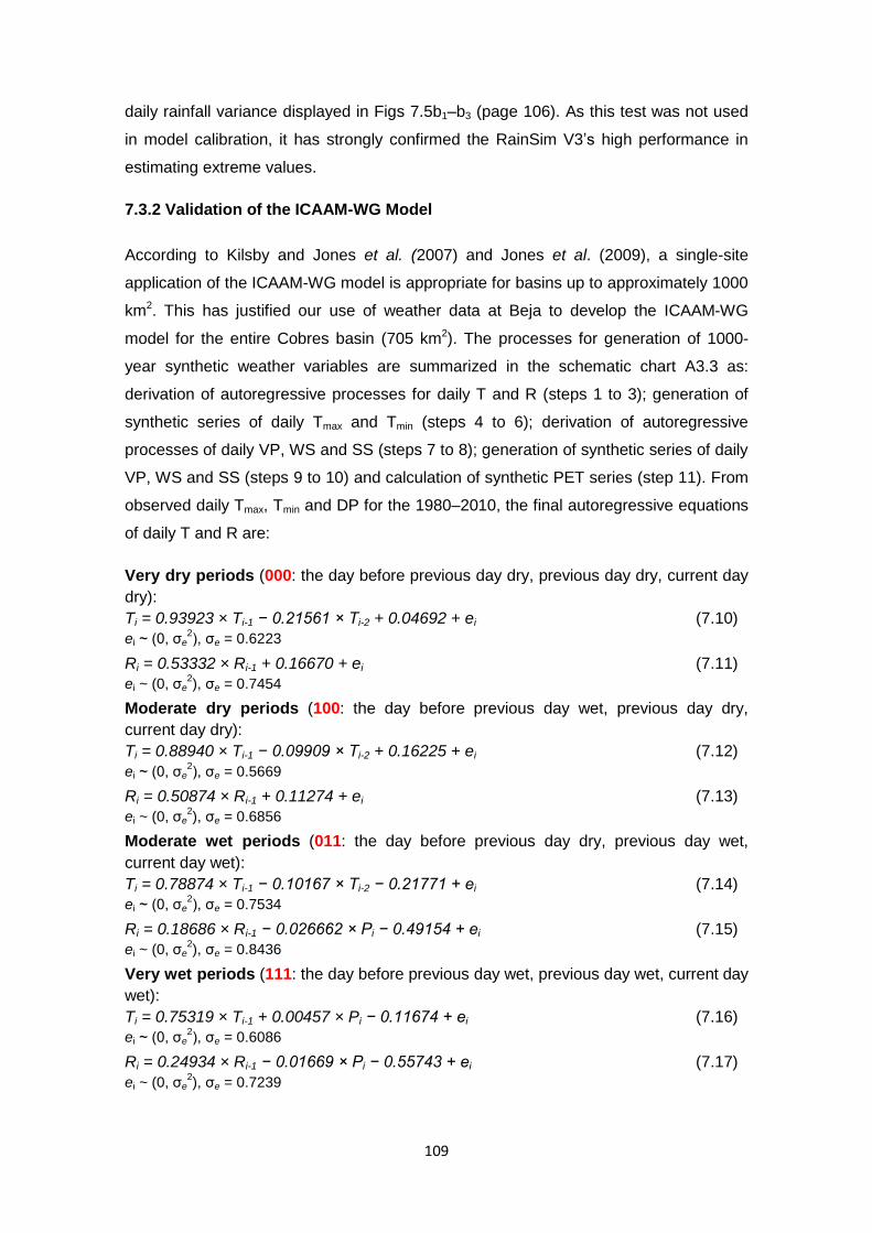
109
daily rainfall variance displayed in Figs 7.5b1–b3 (page 106). As this test was not used
in model calibration, it has strongly confirmed the RainSim V3’s high performance in
estimating extreme values.
7.3.2 Validation of the ICAAM-WG Model
According to Kilsby and Jones et al. (2007) and Jones et al. (2009), a single-site
application of the ICAAM-WG model is appropriate for basins up to approximately 1000
km2. This has justified our use of weather data at Beja to develop the ICAAM-WG
model for the entire Cobres basin (705 km2). The processes for generation of 1000-
year synthetic weather variables are summarized in the schematic chart A3.3 as:
derivation of autoregressive processes for daily T and R (steps 1 to 3); generation of
synthetic series of daily Tmax and Tmin (steps 4 to 6); derivation of autoregressive
processes of daily VP, WS and SS (steps 7 to 8); generation of synthetic series of daily
VP, WS and SS (steps 9 to 10) and calculation of synthetic PET series (step 11). From
observed daily Tmax, Tmin and DP for the 1980–2010, the final autoregressive equations
of daily T and R are:
Very dry periods (000: the day before previous day dry, previous day dry, current day
dry):
Ti = 0.93923 × Ti-1 − 0.21561 × Ti-2 + 0.04692 + ei (7.10)
ei ~ (0, σe2), σe = 0.6223
Ri = 0.53332 × Ri-1 + 0.16670 + ei (7.11)
ei ~ (0, σe2), σe = 0.7454
Moderate dry periods (100: the day before previous day wet, previous day dry,
current day dry):
Ti = 0.88940 × Ti-1 − 0.09909 × Ti-2 + 0.16225 + ei (7.12)
ei ~ (0, σe2), σe = 0.5669
Ri = 0.50874 × Ri-1 + 0.11274 + ei (7.13)
ei ~ (0, σe2), σe = 0.6856
Moderate wet periods (011: the day before previous day dry, previous day wet,
current day wet):
Ti = 0.78874 × Ti-1 − 0.10167 × Ti-2 − 0.21771 + ei (7.14)
ei ~ (0, σe2), σe = 0.7534
Ri = 0.18686 × Ri-1 − 0.026662 × Pi − 0.49154 + ei (7.15)
ei ~ (0, σe2), σe = 0.8436
Very wet periods (111: the day before previous day wet, previous day wet, current day
wet):
Ti = 0.75319 × Ti-1 + 0.00457 × Pi − 0.11674 + ei (7.16)
ei ~ (0, σe2), σe = 0.6086
Ri = 0.24934 × Ri-1 − 0.01669 × Pi − 0.55743 + ei (7.17)
ei ~ (0, σe2), σe = 0.7239

110
Dry wet transition (01: previous day dry, current day wet):
Ti = 0.69150 × Ti-1 − 0.05977 + ei (7.18)
ei ~ (0, σe2), σe = 0.6443
Ri = 0.34515 × Ri-1 − 0.01599 × Pi − 0.55633 + ei (7.19)
ei ~ (0, σe2), σe = 0.8338
Wet dry transition (10: previous day wet, current day dry):
Ti = 0.70959 × Ti-1 − 0.14613 + ei (7.20)
ei ~ (0, σe2), σe = 0.6299
Ri = 0.40933 × Ri-1 + 0.08359 + ei (7.21)
ei ~ (0, σe2), σe = 0.7090
As indicated in equations (7.10)–(7.21), the autoregressive process of temperature for
days of type 000 is different from that for days of type 100, and similarly differences
can be identified between days of types 011 and 111. This may confirm the necessity
of the six transition states’ classification. The magnitudes of coefficients of the mean
temperature for the day before previous day have implicated the possible existence of
second-order autoregressive process of temperature for the days of types 000, 100
and 011. The magnitudes of coefficients of current day rainfall for days of types 011
and 111 are comparable with that for days of type 01, which signifies the importance of
including the influence of current day rainfall on the current day temperature.
Nevertheless, the validation of the weather generator simulations for the control period
will demonstrate the final effects.
The 1000-year synthetic series of Tmax and Tmin for control period are then generated by
applying the 1000-year synthetic DP at Beja into the equations (7.10) to (7.21) and
putting back the seasonal variation of daily T and R. From observed daily T, R, VP, WS,
SS and DP for 1981–2004, the final autoregressive equations are obtained:
Vapour pressure:
VPi = 0.34725 × Ti − 0.30440 × Ri + 0.01151 × Pi + 0.50615 × VPi-1 − 0.01865 + ei
(7.22)
ei ~ (0, σe2), σe = 0.6016
Wind speed:
WSi = − 0.11254 × Ti − 0.13132 × Ri + 0.02809 × Pi + 0.45741 × WSi-1 − 0.04873 + ei
(7.23)
ei ~ (0, σe2), σe = 0.8047
Sunshine duration:
SSi = − 0.03586 × Ti + 0.54979 × Ri + 0.12942 × SSi-1 + ei (7.24)
ei ~ (0, σe2), σe = 0.7698
The 1000-year synthetic series of daily VP, WS and SS for the control period are then
generated by applying standard anomalies of synthetic daily T and R, the 1000-year

111
synthetic DP into the equations (7.22) to (7.24) and putting back their respective
seasonal variations. Finally, the 1000-year synthetic daily PETs are computed from
FAO Penman-Monteith equation. To generate three replicates, steps 4 to 6 and 9 to 11
of A3.3 are required to be repeated three times.
To validate the ICAAM-WG model, the 3000-year synthetic weather variables are
divided into 100 30-year series. The 3 replicates of 1000-year simulation can be treated
as 100 30-year simulations. For each 30-year series, average daily Tmax, Tmin, VP, WS,
SS and PET are evaluated for all the 24 half monthly periods. The performance of the
ICAAM-WG in reproducing the mean climatology at Beja is assessed in Figs 7.7a–f
(page 112), by comparing the observed averages of the weather variables (blue circles)
with the range (red error bar with two standard deviation range) estimated from the 100
simulations. It is shown that the annual cycles of average daily Tmax, Tmin, VP, WS and
SS are all well represented throughout the year although slight overestimation of Tmax
and SS and underestimation of WS in summer are identified. Consequently, the annual
cycle of PET is skillfully reproduced with a little overestimation in summer. Overall, the
synthetic weather variables are in good agreement with the observed values.
7.4 Results of Future Climate Simulations
7.4.1 Simulation of Future Precipitation
The projected monthly rainfall statistics MDP, VarDP, SkewDP, PdryDP1.0 and L1ACDP for
the future time-slice, 2041–2070, for Beja and the 7 rain gauges at Cobres basin (Fig
7.1, page 95) are estimated by using the CF approach described in Section 7.2.4. The
projected annual cycles of hourly rainfall statistics such as VapHP, SkewHP and PdryHP0.1
are evaluated based on the projected daily rainfall statistics VarDP, SkewDP, PdryDP1.0
and equations (7.1)–(7.3). The spatial cross correlation between the rain gauges (XCDP)
are assumed to be constant along time. These statistics are then used to calibrate the
RainSim V3 model and generate three 1000-year climatically stationary simulations for
the future period. Steps, displayed in schematic chart A3.2, for simulation of future
projected multi-site precipitation can be outlined as: preparation of future rainfall
statistics (steps 1 to 3); calibration of RainSim V3 (step 4); generation (step 5) and
analysis (step 6) of synthetic rainfall and comparison of projected, fitted and simulated
statistics for the future period with the corresponding observed, fitted and simulated
statistics for control period (step 7).

112
Fig. 7.7 Validation of weather generator (ICAAM-WG) for simulated daily (a) maximum
temperature (Tmax), (b) minimum temperature (Tmin) ), (c) vapour pressure (VP), (d) wind
speed (WS), (e) sunshine duration and (f) potential evapotranspiration (PET) at Beja
station during the control period (1981–2010); the circles indicate the observed weather
statistics, the crosses represent the simulated means of corresponding values and the
error bars represent variability denoted by two standard deviations of the simulated 100
annual means.
The downscaled synthetic rainfall series have projected change of statistics consistent
with the CFs calculated in Section 7.2.4: (1) Monthly MDP, VarDP, (1 – PdryDP1.0) (daily
rainfall occurrence) are projected to decrease in the non-summer months except
January and March; (2) Frontal activities are projected less frequently in autumn and
December but more frequently in January and spring. Figs 7.8 (pages 113–114),
7.9 (pages 115–116) and schematic charts A4.1 and A4.2 illustrate the comparison of
monthly statistics between future and control periods respectively for Beja, Castro
verde, Almodôvar and Trindade stations.
J F M A M J J A S O N D0
1
2
3
4
5
6
7
8
PE
T (
mm
/day)
CTLOBS
CTLSIM
J F M A M J J A S O N D0
2
4
6
8
10
12
14
SS
(hours
)
CTLOBS
CTLSIM
J F M A M J J A S O N D0.0
0.5
1.0
1.5
2.0
2.5
3.0
3.5
4.0
WS
(m
/s)
CTLOBS
CTLSIM
J F M A M J J A S O N D0
5
10
15
20
VP
(hP
a)
CTLOBS
CTLSIM
J F M A M J J A S O N D0
5
10
15
20
25
30
Tm
in ( C
)
CTLOBS
CTLSIM
J F M A M J J A S O N D10
15
20
25
30
35
40T
max
( C
)
CTLOBS
CTLSIM
(a) (b)
(c) (d)
(e) (f)

113
J F M A M J J A S O N D0.0
0.5
1.0
1.5
2.0
2.5
3.0
3.5
4.0
MD
P (
mm
)
CTLOBS
CTLEXP
CTLSIM
FUT
PRJ
FUTEXP
FUTSIM
J F M A M J J A S O N D0
10
20
30
40
50
60
70
Var D
P (
mm
2)
J F M A M J J A S O N D0.0
0.5
1.0
1.5
2.0
2.5
3.0
3.5
4.0
MD
P (
mm
)
J F M A M J J A S O N D-0.2
0.0
0.2
0.4
0.6
0.8
L1A
CD
P
J F M A M J J A S O N D0.5
0.6
0.7
0.8
0.9
1.0
Pdry
DP
1.0
J F M A M J J A S O N D0
5
10
15
20
25
30
35
40S
kew
DP
J F M A M J J A S O N D0
10
20
30
40
50
60
70
Var D
P (
mm
2)
J F M A M J J A S O N D0.0
0.5
1.0
1.5
2.0
2.5
3.0
3.5
4.0
MD
P (
mm
)
J F M A M J J A S O N D-0.2
0.0
0.2
0.4
0.6
0.8
L1A
CD
P
J F M A M J J A S O N D0.5
0.6
0.7
0.8
0.9
1.0
Pdry
DP
1.0
J F M A M J J A S O N D0
5
10
15
20
25
30
35
40
Skew
DP
J F M A M J J A S O N D-0.2
0.0
0.2
0.4
0.6
0.8
L1A
CD
P
J F M A M J J A S O N D0.5
0.6
0.7
0.8
0.9
1.0
Pdry
DP
1.0
J F M A M J J A S O N D0
5
10
15
20
25
30
35
40
Skew
DP
J F M A M J J A S O N D0
10
20
30
40
50
60
70
Var D
P (
mm
2)
(a1) (a2) (a3)
(b1) (b
2)
(b3)
(c1) (c
2)
(c3)
(d1) (d
2)
(d3)
(e1) (e
2)
(e3)

114
Fig. 7.8 Annual cycles of daily (a1, a2 and a3) mean, (b1, b2 and b3) variance, (c1, c2 and c3)
skewness, (d1, d2 and d3) proportion of dry days and (e1, e2 and e3) lag-1 autocorrelation
and hourly (f1, f2 and f3) variance, (g1, g2 and g3) skewness and (h1, h2 and h3) proportion
dry hours for precipitation at the Beja station from the three 1000-year simulations of the
future period (2041–2070) compared to the control period (1981–2010). The observed
(OBS) or projected (PRJ), fitted (EXP) and simulated (SIM) statistics are respectively
shown in solid lines, circles and crosses and in respective colors of blue and red for the
control (CTL) and future (FUT) periods.
J F M A M J J A S O N D0.80
0.85
0.90
0.95
1.00P
dry
HP
0.1
J F M A M J J A S O N D0
30
60
90
120
150
Skew
HP
J F M A M J J A S O N D0.0
0.2
0.4
0.6
0.8
1.0
1.2
1.4
Var H
P (
mm
2)
J F M A M J J A S O N D0.80
0.85
0.90
0.95
1.00
Pdry
HP
0.1
J F M A M J J A S O N D0
30
60
90
120
150
Skew
HP
J F M A M J J A S O N D0.0
0.2
0.4
0.6
0.8
1.0
1.2
1.4
Var H
P (
mm
2)
J F M A M J J A S O N D0.0
0.2
0.4
0.6
0.8
1.0
1.2
1.4
Var H
P (
mm
2)
CTLOBS
CTLEXP
CTLSIM
FUT
PRJ
FUTEXP
FUTSIM
J F M A M J J A S O N D0.80
0.85
0.90
0.95
1.00
Pdry
HP
0.1
J F M A M J J A S O N D0
30
60
90
120
150
Skew
HP
(f1)
(g1)
(h1)
(f2)
(g2)
(h2)
(f3)
(g3)
(h3)

115
J F M A M J J A S O N D0.0
0.5
1.0
1.5
2.0
2.5
3.0
3.5
4.0
MD
P (
mm
)
CTLOBS
CTLEXP
CTLSIM
FUT
PRJ
FUTEXP
FUTSIM
J F M A M J J A S O N D-0.2
0.0
0.2
0.4
0.6
0.8
L1A
CD
P
J F M A M J J A S O N D0.5
0.6
0.7
0.8
0.9
1.0
Pdry
DP
1.0
J F M A M J J A S O N D0
5
10
15
20
25
30
35
40
Skew
DP
J F M A M J J A S O N D0
10
20
30
40
50
60
70
Var D
P (
mm
2)
J F M A M J J A S O N D0.0
0.5
1.0
1.5
2.0
2.5
3.0
3.5
4.0
MD
P (
mm
)
J F M A M J J A S O N D-0.2
0.0
0.2
0.4
0.6
0.8
L1A
CD
P
J F M A M J J A S O N D0.5
0.6
0.7
0.8
0.9
1.0
Pdry
DP
1.0
J F M A M J J A S O N D0
5
10
15
20
25
30
35
40
Skew
DP
J F M A M J J A S O N D0
10
20
30
40
50
60
70V
ar D
P (
mm
2)
J F M A M J J A S O N D0.0
0.5
1.0
1.5
2.0
2.5
3.0
3.5
4.0
MD
P (
mm
)
J F M A M J J A S O N D-0.2
0.0
0.2
0.4
0.6
0.8
L1A
CD
P
J F M A M J J A S O N D0.5
0.6
0.7
0.8
0.9
1.0
Pdry
DP
1.0
J F M A M J J A S O N D0
5
10
15
20
25
30
35
40
Skew
DP
J F M A M J J A S O N D0
10
20
30
40
50
60
70
Var D
P (
mm
2)
(a1) (a2) (a3)
(b1) (b
2)
(b3)
(c1) (c
2)
(c3)
(d1) (d
2)
(d3)
(e1) (e
2)
(e3)

116
Fig. 7.9 Annual cycles of daily (a1, a2 and a3) mean, (b1, b2 and b3) variance, (c1, c2 and c3)
skewness, (d1, d2 and d3) proportion of dry days and (e1, e2 and e3) lag-1 autocorrelation
and hourly (f1, f2 and f3) variance, (g1, g2 and g3) skewness and (h1, h2 and h3) proportion
dry hours for precipitation at the Castro verde station from the three 1000-year
simulations of the future period (2041–2070) compared to the control period (1981–2010).
The observed (OBS) or projected (PRJ), fitted (EXP) and simulated (SIM) statistics are
respectively shown in solid lines, circles and crosses and in respective blue and red
colors for the control (CTL) and future (FUT) periods.
J F M A M J J A S O N D0.80
0.85
0.90
0.95
1.00P
dry
HP
0.1
J F M A M J J A S O N D0
30
60
90
120
150
Skew
HP
J F M A M J J A S O N D0
30
60
90
120
150
Skew
HP
J F M A M J J A S O N D0.0
0.2
0.4
0.6
0.8
1.0
1.2
1.4
Var H
P (
mm
2)
J F M A M J J A S O N D0.80
0.85
0.90
0.95
1.00
Pdry
HP
0.1
J F M A M J J A S O N D0.0
0.2
0.4
0.6
0.8
1.0
1.2
1.4
Var H
P (
mm
2)
J F M A M J J A S O N D0.80
0.85
0.90
0.95
1.00
Pdry
HP
0.1
J F M A M J J A S O N D0
30
60
90
120
150
Skew
HP
J F M A M J J A S O N D0.0
0.2
0.4
0.6
0.8
1.0
1.2
1.4
Var H
P (
mm
2)
CTLOBS
CTLEXP
CTLSIM
FUT
PRJ
FUTEXP
FUTSIM
(f1)
(g1)
(h1)
(f2)
(g2)
(h2)
(f3)
(g3)
(h3)

117
As indicated in these figures, the fitted (red circles) and simulated (red crosses)
monthly rainfall statistics for the future period excellently match their corresponding
projected (in red solid lines) rainfall statistics except for SkewDP and SkewHP in July,
L1ACDP in July and August, VarHP in January, March, November and December and
PdryHP0.1 in months except July, August and September. For SkewDP and SkewHP in
July, the fitted and simulated values are much smaller than the projected ones
indicating that the RainSim V3 model smoothed the extreme rainfall in that month; for
L1ACDP in July and August, the fitted and simulated values are nearly 0 which is a
result from the correction of unrealistic negative values projected by the CF approach.
As explained in Section 7.3.1, the overestimations of fitted and simulated VarHP are due
to the use of intensity scaling field in the STNSRP process, and the overestimations of
PdryHP0.1 are related to the homogeneous rainfall occurrence assumption adopted in
the RainSim V3 model. Overall, the fitted and simulated monthly statistics correspond
well with the projected values indicating a successful validation of the RainSim V3
model for the future climate scenario.
As shown in Figs 7.8 (pages 113–114), 7.9 (pages 115–116) and schematic charts
A4.1 and A4.2, the comparisons of rainfall statistics for future time slice 2041–2070
with those for present time-slice 1981–2010 have displayed an evaluation of climate
change: (1) Future non-summer months excepting January and March will be drier,
especially for December, February, April, May and September (projected MDP is
decreased respectively around 1 and 0.5 mm/day for December and the other four
months), with nearly the same rainfall skewness but lower intensity, variance and
occurrence than those observed or generated for the control period. (2) Future January
and March are different from other wet months, as indicated by CFs in Figs 7.4a–e
(page 103). Future January will be wet with the same rainfall intensity and skewness
but higher variance and lower occurrence than those observed or simulated for the
control period; future March will be wetter, with the same rainfall occurrence and
skewness but slightly higher rainfall intensity (projected MDP is decreased around 0.2
mm/day) and variance, than in the control period. (3) Future summer months will be dry
with the same low rainfall intensity, variance and occurrence, high skewness and
dominated by convective activities as for control climate.
To evaluate climate change impacts on extreme events, Figs 7.10a–d (page 119) and
Tables 7.3a–d (pages 119–120) are presented. Figs 7.10a–d are comparisons of
extreme plots between future and control periods respectively for Beja, Castro verde,
Almodôvar and Trindade stations. It is indicated, in Figs 7.10a–d, that the future high
and medium frequencies extreme events, namely those with return period less than 10

118
years, have nearly the same magnitudes as the observed or simulated ones for the
control period; however, future low frequency extreme events have distinctly higher
magnitudes than those for the control period. The annual maximum daily rainfall is
around 15% or 10 mm (10% or 5 mm) larger for future extreme events, with a return
period between 20 and 50 years (between 10 and 20 years), than those under the
control climate. Tables 7.3a–d have assessed the climate change impacts on
precipitation extreme indices characterizing both wet and dry conditions. These indices
were used in Costa and Soares (2009) in the context of combating desertification
processes in Southern Portugal. SDII is average wet day precipitation (DP >= 1.0 mm);
R5D is highest consecutive 5-day precipitation total; R30 is number of days with daily
precipitation totals above or equal to 30 mm; CDD is maximum number of consecutive
dry days (DP < 1.0 mm); FDD is number of dry spells (consecutive period with at least
8 dry days, DP < 1.0 mm); AII is average dry day precipitation (DP < 10 mm). The
results, in Tables 7.3a–d, have shown that in the future: (1) high frequency rainfall
events and droughts are slightly drier or remain the same; (2) extreme rainfall events
and droughts are more intense and severe. In Tables 7.3a–b, respectively at 5th and
50th percentiles of the future climate, the SDII decreases around 6% and 1% (or 0.5
and 0.1 mm); the R5D decreases around 6% (or 2.4 mm) and increases 2% (or 1.6
mm); the R30 remains unchanged; the CDD increases around 10% and 5% (or 4 days);
the FDD decreases 13% and 9% (or 1) and the AII decreases 17% and 20% (or 0.1
mm). In Tables 7.3c–d, for future climate respectively at 95th and 98th percentiles, the
SDII decreases around 3% and 4% (or 0.3 and 0.5 mm); the R5D increases around 8%
and 7% (or 9.5 and 9.3 mm); the R30 remains the same; the CDD increases around 13%
and 14% (or 17 and 19 days); the FDD decreases 0 and 1; the AII decreases around
0.1 mm. Considering the large values of R5D and CDD at 95th and 98th percentiles,
their distinct increases under future climate make the extreme rainfall events and
droughts more intense and severe.

119
Fig. 7.10 Gumbel plots comparing observed and simulated extreme daily rainfall for (a)
Beja, (b) Castro verde, (c) Almodôvar and (d) Trindade. The observed rainfall, shown in
black solid squares, is for 1961–2010 at Beja station provided by IPMA and for 1931−2011
at stations Castro Verde, Almodôvar and Trindade provided by SNIRH; the simulated
rainfall was generated by the RainSim V3 model, shown in respective blue and red solid
lines for the control (1981−2010) and future (2041−2070) periods.
Table 7.3a Climate change impacts on moderate precipitation extreme indices (5th
percentile)
Statisticsa
CTL: 1981–2010 (q0.05) FUT: 2041–2070 (q0.05)
Bej Cas Alm Tri Bej Cas Alm Tri
SDII (mm) 7.7 6.8 7.3 6.4 7.2 6.4 6.8 6.0
R5D (mm) 46.6 41.7 45.8 38.0 44.9 38.4 42.3 36.9
R30 (days) 0.0 0.0 0.0 0.0 0.0 0.0 0.0 0.0
CDD (days) 42.0 43.0 42.0 44.0 46.0 47.0 46.0 48.4
FDD (freq.) 8.0 8.0 8.0 8.0 7.0 7.0 7.0 7.0
AII (mm) 0.3 0.3 0.3 0.3 0.2 0.3 0.3 0.2
Note: aThe definitions of the statistics are introduced in section 7.4.1.
-2 -1 0 1 2 3 4 5 60
20
40
60
80
100
120
140
160
180
200
Gumbel reduced variate
An
nu
al m
axim
um
da
ily r
ain
fall
(mm
)
Extreme value plot - Almodovar
2 5 10 20 50 100 200 T
CTL(95%)
CTL(50%)
CTL(5%)
FUT(95%)
FUT(50%)
FUT(5%)
OBS
-2 -1 0 1 2 3 4 5 60
20
40
60
80
100
120
140
160
180
200
Gumbel reduced variate
An
nu
al m
axim
um
da
ily r
ain
fall
(mm
)
Extreme value plot - Trindade
2 5 10 20 50 100 200 T
CTL(95%)
CTL(50%)
CTL(5%)
FUT(95%)
FUT(50%)
FUT(5%)
OBS
-2 -1 0 1 2 3 4 5 60
20
40
60
80
100
120
140
160
180
200
Gumbel reduced variate
An
nu
al m
axim
um
da
ily r
ain
fall
(mm
)
Extreme value plot - Castro verde
2 5 10 20 50 100 200 T
CTL(95%)
CTL(50%)
CTL(5%)
FUT(95%)
FUT(50%)
FUT(5%)
OBS
-2 -1 0 1 2 3 4 5 60
20
40
60
80
100
120
140
160
180
200
Gumbel reduced variate
An
nu
al m
axim
um
da
ily r
ain
fall
(mm
)
Extreme value plot - beja
2 5 10 20 50 100 200 T
CTL(95%)
CTL(50%)
CTL(5%)
FUT(95%)
FUT(50%)
FUT(5%)
OBS
(a) (b)
(c) (d)

120
Table 7.3b Climate change impacts on moderate precipitation extreme indices (50th
percentile)
Statisticsa
CTL: 1981–2010 (q0.50) FUT: 2041–2070 (q0.50)
Bej Cas Alm Tri Bej Cas Alm Tri
SDII (mm) 9.4 8.4 9.0 7.9 9.3 8.2 8.9 7.8
R5D (mm) 72.2 66.3 74.0 61.5 75.8 67.0 75.0 62.5
R30 (days) 2.0 1.0 2.0 1.0 2.0 1.0 2.0 1.0
CDD (days) 74.0 75.0 75.0 80.0 78.0 79.0 78.0 84.0
FDD (freq.) 11.0 11.0 11.0 11.0 10.0 10.0 10.0 10.0
AII (mm) 0.5 0.5 0.5 0.5 0.4 0.4 0.4 0.4
Table 7.3c Climate change impacts on moderate precipitation extreme indices (95th
percentile)
Statisticsa
CTL: 1981–2010 (q0.95) FUT: 2041–2070 (q0.95)
Bej Cas Alm Tri Bej Cas Alm Tri
SDII (mm) 11.6 10.4 11.2 9.8 11.8 10.7 11.6 10.1
R5D (mm) 117.5 115.0 128.6 104.7 131.4 122.1 139.1 111.0
R30 (days) 5.0 4.0 4.0 3.0 5.0 3.0 4.0 3.0
CDD (days) 125.0 128.0 126.0 128.0 142.0 142.0 143.0 147.7
FDD (freq.) 14.0 14.0 14.0 14.0 14.0 14.0 14.0 13.0
AII (mm) 0.7 0.7 0.7 0.7 0.6 0.6 0.6 0.6
Table 7.3d Climate change impacts on moderate precipitation extreme indices (98th
percentile)
Statisticsa
CTL: 1981–2010 (q0.98) FUT: 2041–2070 (q0.98)
Bej Cas Alm Tri Bej Cas Alm Tri
SDII (mm) 12.2 11.0 11.9 10.3 12.6 11.4 12.4 10.8
R5D (mm) 136.6 133.5 152.8 120.8 150.5 142.8 160.2 127.2
R30 (days) 6.0 5.0 5.0 4.0 5.0 4.0 5.0 4.0
CDD (days) 140.0 141.0 140.6 142.6 161.0 160.0 160.0 160.6
FDD (freq.) 15.0 15.0 15.0 15.0 14.0 14.0 14.0 14.0
AII (mm) 0.8 0.8 0.8 0.8 0.7 0.7 0.7 0.7

121
7.4.2 Simulation of Future PET
The three 1000-year climatically stationary synthetic rainfall series, generated in
Section 7.4.1, for future time-slice 2041–2070 at Beja is used to condition the ICAAM-
WG model to generate three 1000-year climatically stationary time series of weather
variables to compute future PET for Cobres basin. The projected annual cycles of
mean and variance of daily T and R for future period are estimated based on the CF
approach introduced in Section 7.2.4. The future 24 half months mean and variance of
daily VP, WS and SS are assumed to be the same as observed, because the
prediction of daily VP and WS is highly uncertain and maximum SS cannot increase.
Following schematic chart A3.4, steps for getting future synthetic daily PET at Beja are:
preparation of future temperature statistics (steps 1 to 3); generation of synthetic series
of future daily Tmax and Tmin (steps 4 to 6); generation of synthetic series of future daily
VP, WS and SS (steps 7 to 8) and calculation of synthetic future PET series (step 9).
Steps 4–9 are repeated three times to get three replicates of 1000-year synthetic future
PET.
Figs 7.11a–e (page 122) show that the 24 half monthly means of simulated future
synthetic daily Tmax, Tmin, VP, WS and SS correspond well with the expected values
except for some slight overestimation of Tmax and SS and underestimation of WS in
summer. This has validated the ICAAM-WG model in reproducing the projected future
mean climatology at Beja. It is shown, in Fig 7.11a–b, that the projected future Tmax and
Tmin increases respectively around 2–4 and 1.5–3 °C throughout the year, which
displays good agreement with the CFs evaluated in Section 7.2.4. Finally, the projected
future synthetic daily PET, Fig 7.11f, increases substantially in May and summer
(around 1.0 mm/day) and relatively less in other months (around 0.4 mm/day).

122
Fig. 7.11 Comparison of the annual cycless of observed (1981–2010: blue circles) and
future (1981–2010: red crosses, black circles) daily (a) maximum temperature (Tmax) and
(b) minimum temperature (Tmin), (c) vapour pressure (VP), (d) wind speed (WS), (e)
sunshine duration (SS) and (f) potential evapotranspiration (PET) at Beja station; the
circles indicate the observed or expected future weather statistics, the crosses represent
the simulated means of corresponding values and the error bars represent variability
denoted by two standard deviations of the simulated 100 annual means.
7.5 Discussion
The three 1000-year climatically stationary synthetic hourly rainfall series were
generated by the RainSim V3 model, for Beja and the other 7 rainfall stations at Cobres
basin, based on the observed statistics and projections of climate derived from the CF
approach (Kilsby and Jones et al., 2007) and RCM model METO-HC_HadRM3Q0
output provided by the ENSEMBLES project for the A1B emission scenario,
respectively for the control (1981–2010) and future (2041–2070) time-slices. The
ICAAM-WG model was developed at Beja station based on Kilsby and Jones et al.
J F M A M J J A S O N D0
1
2
3
4
5
6
7
8
PE
T (
mm
/day)
CTLOBS
FUTWG
J F M A M J J A S O N D0
2
4
6
8
10
12
14
SS
(hours
)
FUTEXP
=CTLOBS
FUTWG
J F M A M J J A S O N D0.0
0.5
1.0
1.5
2.0
2.5
3.0
3.5
4.0
WS
(m
/s)
FUTEXP
=CTLOBS
FUTWG
J F M A M J J A S O N D0
5
10
15
20
VP
(hP
a)
FUTEXP
=CTLOBS
FUTWG
J F M A M J J A S O N D0
5
10
15
20
25
30
Tm
in ( C
)
CTLOBS
FUTEXP
FUTWG
J F M A M J J A S O N D10
15
20
25
30
35
40T
max
( C
)
CTLOBS
FUTEXP
FUTWG
(a) (b)
(c) (d)
(e) (f)

123
(2007) with the inclusion of weather types for considering the existence of the long dry
spells and wet spells for southern Portugal. The three 1000-year climatically stationary
synthetic series of daily Tmax, Tmin, VP, WS, SS and FAO Penman-Monteith PET were
then generated, by the ICAAM-WG, respectively for the control and future periods, with
the condition of synthetic daily rainfall at Beja station. The objective of downscaling the
projection of changes derived from the RCM model was achieved in this chapter. The
generated synthetic hourly rainfall and daily PET, for the control and future periods,
serve as input of SHETRAN model (Chapter 8), for the assessment of future climate
change impacts on hydrological and sediment transport processes.
According to our objective of climate downscaling, the evaluation of model performance
should answer whether or not the synthetic series can reproduce well: (1) the spatial
and temporal (inter- and intra-annual) variations of water resources; (2) the magnitude
and occurrence of extremes and persistence for climate scenarios. For synthetic hourly
rainfall series, point (1) was considered in calibration and validation of the RainSim V3
model by evaluation of annual cycle variations of rainfall mean, variance and cross
correlation among stations. Skewness is a third order moment property, very important
for simulation of extreme rainfall events (Cowpertwait, 1998; Burton et al., 2008) and
lag-1 autocorrelation coefficient is crucial for simulation of persistent events such as
long dry spells (Jones et al., 2009). Therefore, point (2) was considered in model
calibration and validation by assessment of annual cycles of rainfall skewness,
occurrence (or 1–dry probability) and lag-1 autocorrelation. In addition, extreme value
plots, not included in calibration but in validation, were evaluated for consideration of
point (2). As for the synthetic daily PET series, since it was conditioned by synthetic
daily precipitation and mainly influences point (1), the validation of the ICAAM-WG
model was concluded from evaluation of 24 half monthly means of daily PET and its
determinant factors such as Tmax, Tmin, VP, WS and SS.
The rainfall and PET simulations for control climate scenario are very satisfactory. The
RainSim V3 model accurately reproduced monthly MDP, mostly well represented
monthly VarDP and VarHP and reasonably simulated the seasonality of rainfall cross-
correlation properties. The annual cycles of SkewDP, PdryDP1.0, L1ACDP and SkewHP
were well reproduced in spite of the spatially uniformity assumed in the RainSim V3
model (Burton et al., 2008). The annual cycles of PdryHP0.1 were well reproduced in
summer but slightly overestimated in other months (around 5% to 7%) due to the
homogeneity of rainfall occurrence assumed in the model (Burton et al., 2010b). The
ability of the RainSim V3 model in reproducing the realistic rainfall extremes was also
demonstrated for stations with long records of daily rainfall series. The ICAAM-WG

124
model represented well the 24 half months means of Tmax, Tmin, VP, WS, SS and PET,
with slight overestimations of Tmax, SS and PET and underestimation of WS in summer.
Overall, the RainSim V3 and ICAAM-WG models have the capacity of reproducing
synthetic hourly rainfall and daily PET series in conformity to our objectives.
The future climate simulations have shown that the future rainfall is projected to
decrease (around 0.2–0.9 mm/day) in non-summer months especially in December
(around 0.9 mm/day) and in February, April, May and September (around 0.5 mm/day),
increase slightly (around 0.2 mm/day) in March and not change in January and
summer months. Future high frequency events are projected to almost not change, but
future low frequency events such as extreme rainfall events and droughts are projected
to be more intense and severe, around 10%–15% larger than those from the control
period. In summary, future climate is projected to decrease in mean and increase in
extremes. This is consistent with Rajczak et al. (2013), concerning the projected
change of precipitation climate between time-slices 1970–1999 and 2070–2099 for
southern Europe from 10 RCMs provided by the ENSEMBLES project. Future PET is
projected to increase in May and summer around 1 mm/day and in other months
around 0.4 mm/day. The projected decrease in mean daily precipitation and large
increase in PET is expected to deteriorate summer drought, lower the water resources
availability throughout the year and probably accelerate desertification process in
southern Portugal. Therefore, the downscaled climate scenarios are used in Chapter 8
to evaluate the potential impact of climate change on hydrological processes and
sediment transportation at Cobres basin.

125
8. Assessment of Future Climate Change Impacts
Assessment of future climate change impacts are carried out for Cobres basin in this
chapter based on SHETRAN simulations under control (1981–2010) and future (2041–
2070) climates by using the three 1000-year hourly rainfall and daily PET generated in
Chapter 7 and the calibrated SHETRAN parameters derived in Chapter 5. This chapter
begins with a short introduction, and then the methodology is presented. The
evaluations of climate change impacts are carried out in terms of hydrological
processes and sediment transport, with the aim of answering the following three issues:
(1) How much impact would future climate change have on the available water
resources at Cobres basin? (2) How much impact would if have for extreme events? (3)
How much impact would if have for basin sediment yield? Finally, a short discussion is
given in reply to the questions.
8.1 Introduction
In the last decade, the average temperature over continental Europe that is 1.3 °C
warmer than the preindustrial level marked the highest record since preindustrial era
(EEA 2012); and the precipitation has decreased in southern Europe with consequent
decreases in river flows and increases in the frequency and intensity of droughts (EEA
2012). The decreasing water availability has been observed (EEA 2012) and
Seneviratne et al. (2012) concluded with medium confidence that since the 1950s
southern Europe has experienced a trend to more intense and longer droughts.
Regional climate models from the PRUDENCE (Christensen et al. 2007) and
ENSEMBLES (van der Linden and Mitchell 2009) projects have also projected an
exacerbated water stress in southern Europe for future (Blenkinsop and Fowler 2007;
Heinrich and Gobiet 2012; Majone et al., 2012; Forzieri et al., 2013; Fraga et al., 2013;
Hagemann et al., 2013; Rajczak et al., 2013). Climate change impacts are required to
be assessed with better confidence to provide stakeholders with more suitable
adaptation measures, because the increase of temperature and decrease of water
availability would bring about catastrophic economic losses mainly due to the increase
in energy demand for cooling and the reduction in hydropower generation and
agricultural production (EEA 2012). For example, the considerable reductions in river
flow during the 2004–2005 drought (Santos et al., 2007) across the Iberian Peninsula
caused a total estimate of EUR 883 million, equivalent to 0.6% of GDP (Demuth 2009;
EEA 2012).

126
Studies of climate change impacts on southern Europe have not reached consensus
conclusion about the extreme events (EEA 2012; Seneviratne et al., 2012). Future
precipitation extremes may increase in Iberia Peninsula (Rajczak et al., 2013), but
fluvial flood extremes may decrease or increase depending on the domain, climate
model and greenhouse gas emission scenario (Feyen et al., 2012; Rojas et al., 2012).
These studies are all based on direct use of simple bias-correction of RCM model data
and the conclusions were derived from extreme value analysis of 30 data points;
therefore their results should be interpreted with caution. As climate in Iberia Peninsula
is highly variable in space and time, research of climate change impacts on extreme
events should be evaluated on catchment scale and bias-correction of RCM data
should consider high-order rainfall statistics that are related to the extreme events.
This study mainly concerns future climate change impacts on southern Portugal where
annual rainfall is around 400─900 mm (Ramos and Reis 2002) and with large intra-
and inter-annual variability (Corte-Real et al., 1998; Mourato et al., 2010). Climate
studies in this region are mainly focused on water scarcity and drought-related aspects,
which does not exclude the importance of future climate change impacts on extreme
events, not only because of their contribution in sediment transport but also in terms of
their consequences in catastrophic losses. In the 1876 extreme event, the Guadiana
river branch in Mértola raised 25 meters on December 14th, 1876 and the extreme
discharge lasted 3 days and took away everything in its way (Varino 2011); this would
bring about enormous monetary and life losses, if it had happened now and no
appropriate adaptation measures had been planned and implemented.
The objective of this chapter is to assess future climate change impacts on two aspects:
(1) water availability and sediment yield; (2) extreme discharge and sediment
discharges. The future climate change impacts on available water resources and
sediment yield are evaluated based on the analysis of annual and monthly water
balance components and annual and seasonal flow duration curves. The future climate
change impacts on annual maximum daily discharge and sediment discharge are
assessed by comparing the empirical cumulative probability plots (CDFs), extreme
value plots and fitted theoretical distributions during control and future conditions.
8.2 Methodology
8.2.1 SHETRAN Model Simulation
Climate change impacts on hydrological process and sediment transport are evaluated
using the SHETRAN hydrological model. In Chapter 5, we set up the SHETRAN model

127
based on land-use map from CORINE land cover 2006 (Caetano et al., 2009) and soil
type map from IHERA. Based on model structure and previous study, we configured 28
parameters (22 hydrological parameters and 6 sediment parameters), related with the
two main types of land-use and three main types of soil, to be calibrated. The
automatic calibrations of SHETRAN model by MSCE and NSGA-II have produced
different settings of calibration parameters, all allowing well reproduction of hydrological
processes for both calibration and validation periods. This phenomenon has been well
known as equifinality problem (Beven and Freer 2001). The parameter uncertainty may
result in differences in future climate change impacts. On the other hand, from Chapter
6, we have concluded that SHETRAN model simulations with spatial resolution of 1.0
km grid and temporal resolutions of 1.0 hour rainfall and 1.0 day PET would give better
representation of storm-runoff processes at Cobres basin than those with 2.0 km.
However, due to the limited computing resources, we do not consider the parameter
uncertainty and the 0.5 km and 1.0 km grid resolutions for assessment of future climate
impacts. Instead, we chose 2.0 km grid and selected the set of calibration parameters
derived from Sections 5.5.2 and 5.6.4 and considered them valid for both control and
future climate conditions. In Chapter 7, we have obtained three 1000–year synthetic
hourly rainfall and daily PET respectively under control and future conditions. In this
chapter, the future climate change impacts are evaluated by comparison of the
hydrological and sediment transport processes derived from SHETRAN simulations
driven by those 2 series of 3000–year synthetic rainfall and PET data.
8.2.2 Statistical Methods
Descriptive statistical measures
To evaluate future climate impacts on water resources availability and annual sediment
yield, we extracted the descriptive statistical measures, such as mean, standard
deviation (STD), coefficient of variation (CV), 5th, 50th, 95th, 98th and 99th percentiles
(q0.05, q0.50, q0.95, q0.98 and q0.99), from the empirical frequency distributions of annual
variables like rainfall, PET, AET, subsurface storage (∆S), runoff and sediment yield
under control and future conditions. To avoid compensation effects by averaging over
the year, we compare the annual cycle variations of these variables by using boxplots
(Wilks 2006). Furthermore, to get future climate impacts on the hydrological regime of
Cobres basin, we plotted the flow duration curves, for the whole year and the four
individual seasons, under control and future climate scenarios, using the same
methodologies as described in Davie (2008).

128
Extreme value analysis
We describe extreme events as a collection of annual maxima or block maxima (largest
in a block of around 365 values). In this study, we analyze annual maximum daily
discharge and sediment discharge at Monte da Ponte (outlet) station, under control and
future conditions, to assess whether the frequency and magnitude of extreme storm
events are likely to increase as a result of climate change and quantify the possible
changes. The parametric distribution is a compact representation of the empirical
distribution, which facilitates derivation of probabilities for extreme values outside of the
provided data sets, calculation of quantiles for specified probabilities and comparisons
among given extreme distributions. The annual maxima of daily discharge and
sediment discharge are generally heavy tailed and may be described by the
generalized extreme value (GEV) distribution (Stedinger et al., 1993; Katz et al., 2002;
Wilks 2006). In this study, the distribution of extreme events is fitted by the trial-and-
error method, and two steps are required: (1) a GEV distribution is fitted to the data,
and then the probability plot and goodness-of-fit tests decide whether the fit is
appropriate as described by Stedinger et al. (1993); (2) the L-moment diagram is used
to confirm the goodness-of-fit or further investigate the possible distributions consistent
with the available data set. If GEV distribution appears inconsistent with the data,
alternative distributions, suggested by the L-moment diagram, are fitted to the data and
probability plots and goodness-of-fit tests distinguish the most appropriate distribution
from the others. The cumulative distribution functions (CDFs) of GEV, gamma and
three-parameter lognormal distributions are shown in Appendix 5.
The fitting of data to specified distributions can be carried out by using either the
maximum likelihood method (Wilks 2006) or the L-moment method (Hosking 1990;
Hosking and Wallis 1997). We use the matlab functions in statistic toolbox (version
R2013a) developed by the MathWorks Company to fit the data by the former method
and the R functions in the lmom package (version 2.1) developed by Hosking to do the
fitting by the latter method. Then, we select the better one by comparison of the derived
probability plots. Two goodness-of-fit tests, namely the Lilliefors test and the Filliben
test, described in Wilks (2006) are applied. In the Lilliefors test, the test statistic is set
as Dn the largest absolute difference between empirical and fitted cumulative
probabilities (equation 8.1). The null hypothesis is that the data were drawn from the
distribution being tested, and a sufficiently large discrepancy will result in the null
hypothesis being rejected. Statistical simulation is used to derive the critical value of Dn.
We generate 1000 samples, with the length of tested data, from the tested distribution,
by using corresponding matlab functions and calculate Dn for each of 1000 samples.

129
The α-level critical value is then approximated as the (1- α) quantile of the 1000
synthetic Dn.
𝐷𝑛 = max𝑥|𝐹𝑛(𝑥) − 𝐹(𝑥)| (8.1)
Where Fn(x) is the empirical cumulative probability, estimated as Fn(x(i)) = i/n for the ith
smallest data value; and F(x) is the theoretical cumulative distribution function
evaluated at x.
The test statistic of the Filliben test is the correlation between the empirical quantiles x(i)
and the quantiles from the function of tested distribution Φ-1(pi), with pi estimated using
equation 8.2 which approximate the cumulative probability for the ith order statistic. The
null hypothesis is that the data were drawn from the tested distribution, and if the
correlation is smaller than the appropriate critical value the null hypothesis is rejected.
We generate 1000 samples, with the length of tested data, from the tested distribution
and calculate correlation between empirical and theoretical quantiles for each of the
1000 samples. The α-level critical value of correlation is approximated as the α×100%
quantile of the 1000 synthetic correlations.
𝑝(𝑥(𝑖)) =𝑖−𝑎
𝑛+1−2𝑎, 𝑎 = 0.3175 (8.2)
The L-moment diagram is generated by using functions “lmrd” and “lmrdpoints” in the
lmom package (version 2.1) developed by Hosking.
8.3 Assessment of Future Climate Change Impacts
Future climate change impacts are assessed in terms of hydrological and sediment
transport processes. To indicate the future climate impacts on water resources
availability and sediment yield, Table 8.1 (page 130) and Figs 8.1a─f (page 131) show
the water balance components and sediment yield respectively at annual and monthly
scales; Figs 8.2a─e (page 134) compare flow duration curves for the whole year,
autumn, winter and spring between control and future conditions. To display the future
climate impacts on extreme events, Figs 8.3a─b (page 135) and Figs 8.4a─d (page
137) compare, in different ways, the extreme value plots of annual maximum daily
discharge and sediment discharge between control and future scenarios; Figs 8.5a─d
(page 138) display the theoretical fit of the four empirical extreme value distributions;
Fig 8.6 (page 139), Tables 8.2a─b (page 141) and Tables 8.3a─b (page 141) indicate
the results of goodness-of-fit tests for the proposed distribution fits; and finally Figs
8.7a─b (page 140) show histograms and parameters of the best distribution fits.

130
8.3.1 Future Climate Change Impacts on Water Availability and Sediment Yield
Annual water balance components and sediment yield
Table 8.1 shows the statistics for evaluation of climate change impacts on catchment
average changes in mean, standard deviation, coefficient of variation, 5th, 50th, 95th 98th
and 99th percentiles of the annual rainfall, PET, AET, subsurface storage, runoff and
sediment yield. It is indicated that future (2041─2070) basin average annual rainfalls
are decreased around 80─90 mm or 10%─30% for high, medium and low frequency
extremes. Together with the 200 mm or 15% increase of annual PETs, the future
annual runoffs are projected to decrease around 8─88 mm or 30%─80%, with 30%, 60%
and 80% respectively for extremely wet, medium wet and extremely dry years;
consequently, the future annual sediment yields are projected to decrease around
0.26─2.13 t ha-1 year-1 or 30%─87%, with 30%, 55% and 87% respectively for
extremely wet, medium wet and extremely dry years. Future annual PETs increase
around 200 mm for all probability levels; however, the future annual AETs decrease
around 20─60 mm or 5%─20% with larger decrease associated with less annual
rainfall. AET is determined by PET, crop characteristics and soil water stress condition
(Allen et al. 1998). Because we considered the same land-use types for control and
future conditions, the decrease of AETs reflects the existence of water shortage for
future crops, forests and other plants.
Table 8.1 Statistics for evaluation of climate change impacts on catchment: average changes in mean, standard deviation (STD), coefficient of variation (CV), 5
th, 50
th, 95
th 98
th
and 99th
percentiles (q0.05, q0.50, q0.95, q0.98 and q0.99) for annual rainfall (P), PET, AET, subsurface storage (∆S), runoff (R) and sediment yield (SY)
Annual statistics
CTL period: 1981–2010 (FUT period: 2041–2070)
P(mm) PET(mm) AET(mm) ∆S(mm) R(mm) SY(t ha-1
year-1
)
Mean 474 (386) 1257 (1453) 376 (335) 2 (2) 96 (48) 2.35 (1.29)
STD 104 (102) 27 (27) 40 (50) 24 (22) 68 (49) 1.68 (1.26)
CV 0.22 (0.27) 0.02 (0.02) 0.11 (0.15) 13.0 (9.82) 0.70 (1.01) 0.71 (0.98)
q0.05 315 (228) 1213 (1408) 309 (251) -37 (-36) 10 (2) 0.30 (0.04)
q0.50 467 (382) 1257 (1452) 377 (334) 2 (2) 85 (33) 2.04 (0.91)
q0.95 654 (561) 1301 (1497) 440 (416) 42 (38) 227 (144) 5.57 (3.72)
q0.98 708 (613) 1312 (1509) 454 (435) 53 (46) 270 (182) 6.78 (4.94)
q0.99 738 (661) 1322 (1521) 463 (445) 60 (53) 295 (212) 7.63 (5.50)

131
Monthly water balance components and sediment yield
Figs 8.1a─f display the boxplots for annual cycles of monthly rainfall, PET, subsurface
storage change, AET, runoff and sediment yield under control and future scenarios.
Fig. 8.1 Boxplots showing the annual cycles of monthly rainfall (a), PET (b), change of
subsurface storage (∆S) (c), AET (d), runoff (e) and sediment yield (f) under control (blue)
and future (red) climate conditions. The small circles embedded with black dots
represent the median value for each month, the lower (upper) limits of the compacted
boxes represent the first quartile q0.25 (third quartile q0.75), the lower (upper) limits of the
whiskers represent the “q0.25 – 1.5 × (q0.75 – q0.25)” (“q0.75 + 1.5 × (q0.75 – q0.25)”) and the
circles below the lower whiskers (above the upper whiskers) represent outliers.
J F M A M J J A S O N D
-50
0
50
100
150
Month
S
(m
m)
Comparison of basin average S
CTL
FUT
J F M A M J J A S O N D0
20
40
60
80
100
120
Month
AE
T (
mm
)
Comparison of basin average AET
CTL
FUT
J F M A M J J A S O N D0
50
100
150
200
250
MonthP
ET
o (
mm
)
Comparison of basin average PETo
CTL
FUT
J F M A M J J A S O N D0
50
100
150
200
250
300
350
Month
Ra
infa
ll (m
m)
Comparison of basin average rainfall
CTL
FUT
(a) (b)
(c) (d)
(f) (e)

132
The boxplots in Figs 8.1a─f are plots of five sample quantiles: the lower limit of the
lower whisker, q0.25─1.5×(q0.75─q0.25), the lower limit of the compacted solid box, q0.25,
the median, q0.5, the upper limit of the compacted solid box, q0.75, and the upper limit of
the upper whisker, q0.25+1.5×(q0.75─q0.25). The compacted solid boxes indicate the
Interquartile Ranges (IQRs) or the central 50% of the data and, the locations of the
median, display the measures of symmetry of the data. Outliers are shown in empty
circles that stay above or below the whiskers. We can see from Fig 8.1a that: (1)
monthly rainfalls under both control and future conditions are all right-skewed due to
the existence of large extreme values; (2) future monthly rainfalls decrease in non-
summer months, except for January and March, and the decreases are identified for all
the probability levels which are especially pronounced in September, December,
February, April and May; (3) future January and March are with larger IQRs and
extreme rainfall amounts, although the median value keeps the same in January and
increases slightly in March; (4) future summer months continue with little rainfall and
the extreme rainfall amounts in August decrease distinctly. From Fig 8.1b, we know
that (1) the probability distributions of monthly PETs under both control and future
conditions are symmetric; (2) future monthly PETs increase for all the probability levels
and the increases are larger in May and summer months.
Figs 8.1e─f have shown that monthly runoff and sediment yield at Cobres basin are
highly right-skewed for present and future climates. Under control condition, runoff and
sediment erosion mainly occur in November and winter months, although under
extreme circumstances substantial quantities may be identified in October and spring,
especially in March and April. December and January are the only two months that
may always have runoff generation and sediment yield and with large IQRs and
extreme amounts; November and February may have no runoff and sediment yield at a
probability level of 50% but with unneglectable IQRs and considerable extreme values.
Under future condition, the monthly runoff and sediment yield are much more right-
skewed with all median values of 0, meaning no runoff and sediment yields would
occur all over the year at a probability level of 50%. December and January are the
only two months with non-ignorable amounts of runoff and sediment yield in the future
at a probability level of 50%. Under extreme circumstances, November, December and
January in the future may have destructive amounts of runoff and sediment yield and
future February, March and April may have considerable quantities. As for summer and
September, no runoff and sediment yield is identified for future, even under extreme
conditions; the possible extreme values in August and September under control
condition decrease to zero in the future.

133
Fig 8.1d displays future monthly decrease of AET except for winter months, indicating
future vegetation and crop growths are more water-limited than under control climate.
Fig 8.1c depicts monthly subsurface water increase or decrease under control and
future conditions, which, together with monthly rainfall (Fig 8.1a) and AET (Fig 8.1d),
explains future climate change on monthly runoff (Fig 8.1e) and sediment yield
(Fig 8.1f). Spring is the season with considerable rainfall but nearly no runoff, and
consequently no sediment yield, at Cobres basin for both control and future conditions;
because the rainfall amounts (around 20─50 mm in median) are not sufficient to supply
AETs (around 40─55 mm in median) which leads to subsurface water deficits (around
3─23 mm in median). Summer is a completely dry season with no rainfall but high
subsurface water deficits (around 18─32 mm in median) which well explains the
complete absence of runoff and sediment yield. Under control condition, September is
the first month with considerable rainfall after the summer drought, however, this
rainfall amount (around 18 mm in median) is completely used in AET dispense (around
22 mm in median), therefore no runoff and consequently no sediment yield is produced;
future September is even drier with only a little rainfall (around 8 mm in median) quite
insufficient for supplying AET (around 17 mm in median) and produce runoff and
sediment yield. October is the first month with abundant rainfall (around 50 mm in
median) sufficient to provide AET (around 25 mm in median) and refresh subsurface
water storage (around 25 mm in median) under both control and future conditions;
however, no runoff is generated in this month, consequently no sediment yield is
produced. November and winter are the only months with the wettest soil moisture
conditions and the lowest PETs in the year. Under the control condition, there is 50%
probability that runoff, and consequent sediment yield may be generated in November
and February; however as a consequence of precipitation decrease, nearly no runoff
and sediment yield are produced in the future. December is the month with most runoff
and sediment yield, under either control (around 54 mm runoff and 1.4 t ha-1 sediment
yield in 75th percentile) or future (around 20 mm and 0.6 t ha-1 in 75th percentile)
conditions, due to the largest rainfall amounts and smallest AET dispense; similarly,
January is the month with second largest runoff generation and sediment yield. Under
future condition, precipitation decreases in December and AET increases in both
December and January, which leads to a probability level of 50% for runoff generation
and sediment yield in these two months. Nevertheless, extreme runoff and sediment
yield may occur mainly in November, December and January, probably with largest
magnitude, or secondarily in February, March and April, probably with moderate
magnitude. The future extreme values, shown in Figs 8.1e─f, seem to be much smaller
than the control ones, for which further investigations are shown in the next section.

134
Annual and seasonal flow duration curves
Fig 8.2a and Fig 8.2b indicate annual and seasonal flow duration curves under
respective control and future conditions; comparisons between control and future are
respectively shown in Fig 8.2c, Fig 8.2d, Fig 8.2e and Fig 8.2f for the whole year,
autumn, winter and spring.
Fig. 8.2 Flow duration curves derived from the three 1000-year SHETRAN hydrological simulations under the (a) control and (b) future conditions, which are shown in blue, green, black, purplish-red and red colors respectively for the whole year, autumn, winter, spring and summer. Comparisons are shown in (c), (d), (e) and (f), with blue representing control and red for future, respectively for the whole year, autumn, winter and spring. The abscissa shows the percentage of flow exceeded and the ordinate indicates flows at outlet of the Cobres basin in a natural log-scale.
0 10 20 30 40 50 60 70 80 90 100-8
-6
-4
-2
0
2
4
6
8
% time flow exceeded
Ln
flo
w (
m3/s
)
CTLwinter
FUTwinter
0 10 20 30 40 50 60 70 80 90 100-8
-6
-4
-2
0
2
4
6
8
% time flow exceeded
Ln
flo
w (
m3/s
)
CTLspring
FUTspring
0 10 20 30 40 50 60 70 80 90 100-8
-6
-4
-2
0
2
4
6
8
% time flow exceeded
Ln
flo
w (
m3/s
)
FUTyear
FUTautumn
FUTwinter
FUTspring
FUTsummer
0 10 20 30 40 50 60 70 80 90 100-8
-6
-4
-2
0
2
4
6
8
% time flow exceeded
Ln
flo
w (
m3/s
)
CTLautumn
FUTautumn
0 10 20 30 40 50 60 70 80 90 100-8
-6
-4
-2
0
2
4
6
8
% time flow exceeded
Ln
flo
w (
m3/s
)
CTLyear
CTLautumn
CTLwinter
CTLspring
CTLsummer
0 10 20 30 40 50 60 70 80 90 100-8
-6
-4
-2
0
2
4
6
8
% time flow exceeded
Ln
flo
w (
m3/s
)
CTLyear
FUTyear
(a) (b)
(c) (d)
(f) (e)

135
Flow duration curve reflects how representative is the water flowing down a river, or
simply a curve of discharge values versus its exceedance probabilities. In this study,
we used daily mean discharge at Monte da Ponte station (basin outlet) to plot these
curves. Under control condition (Fig 8.2a), winter is the wettest season of a year with
discharges higher than 1 m3/s for around 1 month and 20 m3/s for nearly 9 days;
summer is a completely dry season and normally no water is available; spring and
autumn, with nearly the same flow duration curves, are seasons with no flow for most
(~85%) of the time and with discharges larger than 1 m3/s for only around 9 days;
finally, the whole year at Cobres basin is mostly (~80% of time) dry with discharges
larger than 1 m3/s for around 50 days and 2.7 m3/s for around 36 days. Under future
condition (Fig 8.2b), winter is still the wettest season of the year, although much drier
than under control condition (Fig 8.2e), with discharges higher than 1 m3/s for around
15 days and 20 m3/s for nearly 3 days; summer is also completely dry with no
discharge; spring and autumn, drier than under control condition (Fig 8.2d and 8.2f),
with no flow for around 90% of the time and with discharges larger than 1 m3/s for only
around 4─5 days; the whole year, drier than the present climate (Fig 8.2c), is with no
flow for around 90% of the time and with discharges larger than 1 m3/s for only around
25 days and 2.7 m3/s for around 16 days.
8.3.2 Future Climate Change Impacts on Extreme Events
Future climate change impacts on extreme events
Future climate change impacts on extreme events are shown in Figs 8.3a─b and
8.4a─d.
Fig. 8.3 Gumbel plots comparing annual maximum daily (a) discharge and (b) sediment
discharge for Monte da Ponte gauging station (basin outlet) in blue and red colors
respectively under control (1981−2010) and future (2041−2070) conditions. 5%, 50% and
95% represent the 5th
, 50th
and 95th
percentile of the extremes.
-2 -1 0 1 2 3 4 5 60
100
200
300
400
500
600
Gumbel reduced variate
An
nu
al m
ax d
aily
dis
ch
arg
e (
m3/s
)
Extreme value plot - Monte da Ponte
2 5 10 20 50 100 200 T
CTL(95%)
CTL(50%)
CTL(5%)
FUT(95%)
FUT(50%)
FUT(5%)
-2 -1 0 1 2 3 4 5 60
500
1000
1500
2000
2500
3000
Gumbel reduced variate
An
nu
al m
ax d
aily
se
d d
isch
arg
e (
kg
/s)
Extreme value plot - Monte da Ponte
2 5 10 20 50 100 200T
CTL(95%)
CTL(50%)
CTL(5%)
FUT(95%)
FUT(50%)
FUT(5%)
(a) (b)

136
Figs 8.3a─b were plotted by dividing the 3000-year simulated annual maxima series
into 50 60-year series as described in Section 7.4.1 and displayed in Figs 7.10a─d
(page 119), which were designed to provide information about how the future extreme
runoffs would be changed under future extreme rainfalls. Figs 8.4a─d (page 137) are
derived directly from the 3000-year simulated annual maxima series. Fig 8.4a and Fig
8.4c are cumulative probability plots respectively used to distinctly compare discharges
and sediment discharges for high frequency events under control and future conditions;
Fig 8.4b and Fig 8.4d are used to carry out the comparisons more clearly for medium
and low frequency events. We categorize extreme events by their return periods (T) or
non-exceedance probabilities (P) as five types, namely: high (T ≤ 2 years or P ≤ 0.5),
medium (2 < T ≤ 10 years or 0.5 < P ≤ 0.9), low (10 < T ≤ 20 years or 0.9 < P ≤ 0.95),
very low (20 < T ≤ 50 years or 0.95 < P ≤ 0.98) and extremely low (T > 50 years or P >
0.98) frequency events. It is indicated, in Fig 8.3a and Figs 8.4a─b, that (1) future high,
medium and low frequency flows are respectively decreased around 35%─80% (or
20─35 m3/s), 5%─35% (or 10─30 m3/s) and 3%─5% (or 5─10 m3/s); (2) future very low
and extremely low frequency flows are nearly the same or slightly decreased compared
to their values under control conditions; (3) for extremes in discharge, values smaller
than 200 m3/s, the non-exceedance probabilities are larger in future climate than in
present climate, for those with values larger than 200 m3/s, their probabilities in future
climate are nearly the same as those in present climate. In other words, the future
extremes have discharges of magnitude smaller or similar to those under control
climate and the increases of future rainfall maxima, indicated in Figs 7.10a─d, do not
result in corresponding increases of runoff. Similarly, from Fig 8.3b and Fig 8.4c─d, (1)
future high, medium and low frequency sediment discharges are respectively
decreased around 30%─60% (or 50─70 kg/s), 10%─25% (or 40─60 kg/s) and 1%─5%
(or 6─30 kg/s); (2) future very low and extremely low frequency sediment discharges
are nearly the same or slightly decreased compared to their values under control
conditions; (3) for extremes in sediment discharges, values smaller than 600 kg/s, the
non-exceedance probabilities are larger in future climate than in present climate, for
those with values larger than 600 kg/s, their probabilities in future climate are nearly the
same as those in present climate.

137
Fig. 8.4 Empirical cumulative frequency distribution functions for (a) the annual
maximum daily discharge and (c) the annual maximum daily sediment discharge under
control (CTL) and future (FUT) conditions. Empirical extreme plots for comparison of (b)
annual maximum daily discharge and (d) annual maximum daily sediment discharge
under control and future conditions. The 3000-year synthetic daily discharge and
sediment discharge series were used to derive the plots.
Theoretical fit of empirical extreme value distributions
GEV distributions have been fitted, by using the maximum likelihood and L-moment
methods, to the 3000-year simulated series of annual maximum daily discharge and
sediment discharge under control and future conditions. The results have shown that L-
moment method gave better fits for all of the four cases than the maximum likelihood;
therefore it is adopted and the results are shown in Figs 8.5a─d (page 138) with
Figs 8.5a and 8.5c referring to control condition and Figs 8.5b and 8.5d to future
condition.
0 1 2 3 4 5 60
1
2
3
4
5
6
7
8
9
10
Gumbel reduced variateAn
nu
al m
ax d
aily
se
d d
is (
2
00
kg
/s)
2 5 10 20 50 100 200T
CTL
FUT
10-1
100
101
102
103
0.0
0.1
0.2
0.3
0.4
0.5
0.6
0.7
0.8
0.9
1.0
Annual max daily sed discharge (kg/s)
Cu
mu
lative
pro
ba
bili
ty, P
r(X
x
)
CTL
FUT
0 1 2 3 4 5 60
50
100
150
200
250
300
350
400
450
500
Gumbel reduced variate
An
nu
al m
ax d
aily
dis
ch
arg
e (
m3/s
)
2 5 10 20 50 100 200T
CTL
FUT
(b)
(c) (d)
10-1
100
101
102
103
0.0
0.1
0.2
0.3
0.4
0.5
0.6
0.7
0.8
0.9
1.0
Annual max daily discharge (m3/s)
Cu
mu
lative
pro
ba
bili
ty, P
r(X
x
)
CTL
FUT
(a)

138
Fig. 8.5 Probability distributions of annual maximum daily discharge under (a) control
and (b) future conditions and annual maximum daily sediment discharge under (c)
control and (d) future conditions. The red circles are derived from SHETRAN model
simulations; the blue and black lines are fitted, by using the R functions of the lmom
package (version 2.1), based on postulated distributions, namely generalized extreme
value (GEV), Gumbel or extreme value (EV), gamma and three-parameter lognormal (ln3)
distributions. The blue lines are corresponding best fits.
From visual comparison, we find that GEV distribution fits well the 3000-year simulated
annual maxima series under control condition for all the data ranges and for future
condition it fits well the annual maximum discharges and sediment discharges with
return periods respectively in the ranges of [2, 50] and [2, 200] years.
In order to check the goodness-of-fit and explore possible candidate distributions for
better fit, we plotted the L-moment diagram (Fig 8.6, page 139) for the four annual
maxima series.
(a) (b)
(c) (d)

139
Fig. 8.6 L-moment diagram indicating relationships among L-skewness and L-Kurtosis
for the generalized logistic (GLO), generalized extreme value (GEV), generalized Pareto
(GPA), generalized normal (GNO), Pearson type III (PE3), exponential (E), Gumbel (G),
logistic (L), normal (N) and uniform (U) and the distribution of the 3000-year annual
maximum daily discharge under control (blue circle) and future (red circle) conditions
and the 3000-year annual maximum daily sediment discharge under control (blue cross)
and future (red cross) conditions.
As shown in Fig 8.6, the annual maxima series of simulated flow and sediment
discharge under control condition, indicated in blue circles and crosses, may be well
fitted by the GEV distribution; for future condition, the annual maxima series of
simulated flow, displayed in red circles, may be well fitted by the Pearson type III (or
gamma), generalized Pareto or exponential distributions and the annual maxima series
of sediment discharge, shown in red crosses, may be well fitted by the generalized
normal distribution. Therefore, Fig 8.6 has confirmed the goodness-of-fit of GEV
distribution for annual maxima series under control condition; for future condition, it has
indicated the lack-of-fit of GEV distribution and suggested better options. We visually
tested the goodness-of-fit of the candidate distributions for future condition by making
probability plots and we found that gamma and the three-parameter lognormal
distributions respectively fit well the annual maxima series of simulated discharge and
sediment discharge for all the data ranges, as shown in Figs 8.5b and 8.5d.
The Lilliefors test and the Filliben test have been applied to further test the goodness-
of-fit of proposed distributions shown in Figs 8.5a─d. We applied the two goodness-of-
fit tests to both the whole 3000-year samples and the original three splitted 1000-year
samples. From Lilliefors tests indicated in Table 8.2a (page 141), under control
condition the annual maximum daily discharge series match the GEV distribution at a
significance level of 5%; and under future condition it does not match the GEV
distribution but matches the gamma distribution at a significance level of 5%. According
to Filliben tests shown in Table 8.2b (page 141), under control condition the annual

140
maximum daily discharge series does not match the GEV distribution at a significance
level of 5%; and under future condition it matches neither the GEV distribution nor the
gamma distribution at a significance level of 5%. Similarly, for the annual maximum
daily sediment discharge series, the Lilliefors tests displayed in Table 8.3a (page 141)
shows that under control condition it matches the GEV distribution at a significance
level of 5%, and under future condition it does not match the GEV distribution but
instead match the three-parameter lognormal distribution at a significance level of 5%;
the Filliben tests displayed in Table 8.3b (page 141) show that under control condition it
matches the GEV distribution at a significance level of 5%, and under future condition it
matches both the GEV distribution and the three-parameter lognormal distribution at a
significance level of 5%. It is indicated that the results of the Lilliefors tests are all
consistent with visual fit of goodness-of-fit test for the distributions proposed in Figs
8.5a─d (page 138), which demonstrates the feasibility of representing the empirical
distributions by the proposed theoretical distributions. The results of the Filliben tests
are not always consistent with the visual fits, which may be explained by the non-
resistance property of the Pearson correlation coefficient (Wilks 2006).
Finally, we compared the histograms of fitted distributions in Figs 8.7a─b.
Fig. 8.7 Histograms of fitted distributions for (a) annual maximum daily discharge and (b)
annual maximum daily sediment discharge under control (CTL) and future (FUT)
conditions.
It is found that: (1) The probability density function (PDF) of the future annual maximum
discharge is much more right-skewed with its highest probability density located at 0
m3/s; non-exceedance probabilities of future annual maximum discharges with values
in the range of [0, 200] m3/s are higher and are especially higher for those in the range
of [0, 60] m3/s. (2) The PDF of the future annual maximum sediment discharge is more
right-skewed with its highest probability density located nearer to 0 kg/s; non-
0 1000 2000 3000 40000
100
200
300
400
500
600
Annual max daily sed discharge (kg/s)
Ab
so
lute
fre
qu
en
cy
lognormal(FUT)
=-46.2
lognormal(FUT)
=5.3
lognormal(FUT)
=0.78
GEV(CTL)
=164.4
GEV(CTL)
=120.3
GEV(CTL)
= -0.24
CTL
FUT
0 200 400 600 800 1000 12000
100
200
300
400
500
600
Annual max daily discharge (m3/s)
Ab
so
lute
fre
qu
en
cy
gamma(FUT)
=0.97
gamma(FUT)
=75.2
GEV(CTL)
=64.6
GEV(CTL)
=46.5
GEV(CTL)
= -0.09
CTL
FUT
(a) (b)

141
exceedance probability of future annual maximum discharges with values in the range
of [0, 500] kg/s is higher and it is especially higher for values in the range of [0, 50] kg/s.
Table 8.2a Lilliefors test for annual maximum daily discharge under CTL and FUT conditions
Test Null distribution Dnmax (Crit0.05)
1st
1000 year 2nd
1000 year 3rd
1000 year 3000 year
CTL GEV 0.025 (0.043) 0.025 (0.043) 0.020 (0.043) 0.020 (0.024)
FUT GEV 0.073 (0.042) 0.064 (0.042) 0.065 (0.042) 0.069 (0.024)
FUT gamma 0.028 (0.042) 0.051 (0.044) 0.032 (0.043) 0.035 (0.024)
Table 8.2b Filliben test for annual maximum daily discharge under CTL and FUT conditions
Test Null distribution R (Crit0.05)
1st
1000 year 2nd
1000 year 3rd
1000 year 3000 year
CTL GEV 0.884 (0.991) 0.912 (0.991) 0.917 (0.988) 0.987 (0.996)
FUT GEV 0.912 (0.970) 0.920 (0.976) 0.922 (0.961) 0.991 (0.981)
FUT gamma 0.878 (0.907) 0.885 (0.910) 0.870 (0.899) 0.929 (0.912)
Table 8.3a Lilliefors test for annual max daily sediment discharge under CTL and FUT conditions
Test Null distribution Dnmax (Crit0.05)
1st
1000 year 2nd
1000 year 3rd
1000 year 3000 year
CTL GEV 0.019 (0.041) 0.026 (0.041) 0.021 (0.042) 0.014 (0.025)
FUT GEV 0.039 (0.042) 0.044 (0.042) 0.048 (0.042) 0.046 (0.025)
FUT lognormal 0.025 (0.042) 0.034 (0.043) 0.036 (0.043) 0.033 (0.025)
Table 8.3b Filliben test for annual max daily sediment discharge under CTL and FUT conditions
Test Null distribution R (Crit0.05)
1st
1000 year 2nd
1000 year 3rd
1000 year 3000 year
CTL GEV 0.963 (0.956) 0.988 (0.959) 0.988 (0.952) 0.996 (0.974)
FUT GEV 0.989 (0.927) 0.987 (0.940) 0.986 (0.926) 0.990 (0.944)
FUT lognormal 0.999 (0.973) 0.994 (0.944) 0.980 (0.948) 0.999 (0.987)
8.4 Discussion
Future climate change impacts on water resources availability, annual sediment yield
and annual maximum discharge and sediment discharge were evaluated for Cobres
basin based on SHETRAN hydrological and sediment transport simulations driven by
the downscaled scenarios obtained in Chapter 7 for control (1981─2010) and future
(2041─2070) climates. In the study, we did not consider the possible changes of land-
use in the future; therefore we used the best parameter setting of SHETRAN model,
which is optimized from the available data for the period 2004─2008 by using MSCE

142
and NSGA-II methods, for both climate scenarios. With the aim of assessing future
climate change impacts on available water resources and basin sediment yield, we
compared future annual runoff and sediment yield at high, medium and low frequency
levels with those under control conditions and analyzed the changes by comparing the
annual and monthly water balance components under both climate conditions. In order
to get future climate change impacts on extreme events, we extracted annual
maximum discharge and sediment discharge for both scenarios, carried out the
extreme value analysis by comparison of the empirical distributions and theoretical fits.
Future mean climate is drier with decreased rainfall, increased PET and consequently
decreased runoff and sediment yield. Under future climate, annual rainfall is projected
to decrease around 80─90 mm (or 10%─30%) and annual PET is projected to increase
around 200 mm (or 15%); annual runoffs and sediment yields are projected to
decrease respectively around 8─88 mm (or 30%─80%) and 0.26─2.13 t ha-1 year-1 (or
30%─87%). Annual AET is projected to decrease in the future around 20─60 mm (or
5%─20%) with larger decrease associated with less annual rainfall. The monthly AET
is projected to decrease all over the year except for winter, indicating vegetation and
crop growths are more water-limited in future climate. Spring, summer and early
autumn months are periods with no runoff, and consequently no sediment yield, for
both control and future scenarios, due to the lack of rainfall (in summer months) or the
insufficient rainfall to compensate the water loss from AET and subsurface storage
change. November and winter months are periods with runoff and sediment yield under
control climate; December and January are months with runoff and sediment yield with
occurrence at a probability level of 50% under future climate.
Future wet extremes are more right-skewed with their highest probability density
located near 0. Future annual maximum discharge and sediment discharge are
projected to decrease, respectively around 3%─80% and 1%─60%, for return periods
less than 20 years and the decreases are larger, respectively around 35%─80% and
30%─60, for return periods less than 2 years; annual maxima have the same or slightly
less intensities, for those with return periods larger than 20 years. In other words, for
extremes with discharge (sediment discharge) values smaller than 200 m3/s (600 kg/s),
the non-exceedance probabilities are larger in future climate than in present climate; for
those with values larger than 200 m3/s (600 kg/s), their probabilities in future climate
are nearly the same as those in present climate. Moreover, the series of annual
maximum discharge (sediment discharge), under control condition, follows the GEV
distribution with location parameter of 64.6 m3/s (164.4 kg/s), scale parameter of 46.5
m3/s (120.3 kg/s) and shape parameter of -0.09 (-0.24); under future condition, the

143
series of annual maximum discharge follows the gamma distribution with scale
parameter of 75.2 m3/s and shape parameter of 0.97 and the series of annual
maximum sediment discharge follows the three-parameter lognormal distribution with
location parameter of -46.2 kg/s, mean of 5.3 kg/s and standard deviation of 0.78 kg/s.
In summary, future droughts should be put in the top list of climate adaptation
measures for water supply and desertification combating problems in southern Portugal;
and future wet extremes should not be ignored, but well anticipated as the larger
extremes maintain similar magnitude to those under control conditions. This has
confirmed the increasingly concerns of water scarcity and drought problems for future
(EEA 2012; Seneviratne et al., 2012), and provided a comprehensive evaluation of
future climate change impacts on extreme events in southern Portugal. However,
considering the limitation of this work, further studies are expected to evaluate
uncertainties involved in assessment of future climate change impacts on hydrological
process and sediment transport, which result from the variability in internal
parameterization of GCMs and RCMs, greenhouse gas emission scenarios,
downscaling methods, hydrological model structure and hydrological parameter setting.

144

145
9. Conclusions and Expectations
9.1 Summary
In this study, SHETRAN hydrological model has been successfully calibrated by using
two global optimization methods MSCE and NSGA-II. It is demonstrated that the fitness,
in descending order from high to low, of the spatial resolutions to the SHETRAN
hydrological simulations at Cobres basin is: 0.5, 1.0 and 2.0 km. The best solutions
from SHETRAN calibrations with NSE of values larger or equal to 0.85 and spatial
resolutions of 1.0 and 2.0 km have been successfully validated, for possible future
applications, by considering the tests of split-sample, differential split-sample, proxy-
basin and multi-site. Due to the limits of computational resources, 2.0 km was selected
as the spatial resolution and the best solution from the MSCE calibration was applied to
the simulations of hydrological scenarios for both control (1981–2010) and future
(2041–2070) climates. In summary, the following aspects can be concluded:
Future projections have presented relatively to the reference period a drier
mean climate, with mean annual rainfall decreased by ~88 mm (19%), mean
annual PET increased ~196 mm (16%) and consequent mean annual runoff
and sediment yield decreased respectively ~48 mm (50%) and ~1.06 t/ha/year
(45%). The future mean annual AET is projected to decrease ~41 mm (11%),
which occurs mainly in spring, indicating a more water-limited future climate for
vegetation and crop growth. Under reference conditions, November to February
is the period in which runoff and sediment yield occur frequently; however, in
future, it is reduced to December and January, with changes in the occurrence
rate of ~50%.
Future projections point to increases in the meteorological drought (scarcity of
precipitation, Tables 7.3a–d, pages 119–120), agricultural drought (reduction in
soil moisture, Figs 8.1a, b and d, page 131) and hydrological drought (reduction
in runoff, Figs 8.1e, page 131, and 8.2c–f, page 134). Moreover, the extreme
droughts are projected to be more intense and severe (Tables 7.3c–d, page
120; Figs 8.1a, b and d, page 131; 8.2c–f, page 134 and Fig 8.4a, page 137).
These impacts demand policymakers to adopt and execute efficient adaptation
measures to avoid the socioeconomic drought. Effect of climate change,
particularly of the increase in temperature, is to reduce productivity, refered in a
paper that used projections done in this thesis (Carvalho et al., 2013).

146
Future projections have displayed a level of around 15% increases in
precipitation extremes with return periods in the range of [20, 50] years but
either slight increase or no change in those with return periods respectively in
the ranges of [10, 20] and [2, 10] years. The increases of precipitation extremes
are in accordance with the results obtained by other authors, e.g. Rajczak et al.
(2013).
Future projections have shown no changes or slight decreases in annual
maximum discharge and sediment discharge for extremes with return periods
larger than 20 years; and both quantities present decreases for extremes with
return periods less than 20 years and the decreases are especially greater for
those less than 2 years. The annual maximum discharge (sediment discharge)
series, under control climate, are projected to follow the GEV distribution with
location parameter of 64.6 m3/s (164.4 kg/s), scale parameter of 46.5 m3/s
(120.3 kg/s) and shape parameter of 0.09 (-0.24); under future climate, the
annual maximum discharge series are projected to follow the gamma
distribution with scale parameter of 75.2 m3/s and shape parameter of 0.97 and
the annual maximum sediment discharge series follows the three-parameter
lognormal distribution with location parameter of -46.2 kg/s, mean of 5.3 kg/s
and standard deviation of 0.78 kg/s.
9.2 Main Achievements
All in all, the main achievements can be identified as follows:
An integrated modelling method has been developed for evaluation of climate
change impacts on water resources, sediment yield and extreme events at a
catchment scale, which can be easily applied to any other catchments.
A quantified evaluation of climate change impacts on an agricultural dominated
basin in southern Portugal has been provided in terms of water resources,
sediment yield and wet and dry extreme events.
The rainfall conditioned weather generator—ICAAM-WG has been developed in
this study based on the modified Climate Research Unit daily Weather
Generator (CRU-WG) (Kilsby and Jones et al., 2007). The development of
ICAAM-WG has considered the climate characteristic of southern Portugal,
namely long dry and wet spells.
For the first time, SHETRAN hydrological model has been successfully
calibrated by using two objective global optimization methods, namely the
MSCE and NSGA-II algorithms.

147
For the first time, the effects of spatial resolution on SHETRAN model
performances have been investigated with the aid of a global optimization
algorithm, which provides objective conclusions.
The capability of SHETRAN hydrological model in simulating water resources
and extreme events under different climate conditions are successfully
demonstrated by the strong validations such as the split-sample test, differential
split-sample test, proxy-basin test and multi-site test.
9.3 Main Limitations of the Work
The main limitations of the work are as follows:
o The uncertainties resulting from GCMs, RCMs, GHGs, statistical downscaling
methods and hydrological models were not considered in the future climate
projections.
o The uncertainties resulting from the SHETRAN hydrological model, such as
model structure uncertainty and parameter uncertainty, were not considered.
o The application of 2.0 km, not the best spatial resolution for Cobres basin, to
the SHETRAN hydrological simulations of climate scenarios may have caused
some levels of underestimations in runoff volumes and peak discharges.
o The bad quality of the observed sediment discharge data may have introduced
substantial errors in the calibration of sediment parameters and consequently in
sediment transport simulations for the climate scenarios.
9.4 Further Research
Further research should be carried out including the following aspects:
The considerations of ensembles of GCMs, RCMs, GHGs, statistical
downscaling methods and hydrological models in future climate projections.
The applications of the state-of-the-art global optimization methods to automatic
calibration of SHETRAN model.
The improvement in sediment measurements.

148

149
10. References
Abbott, M. B., Bathurst, J. C., Cunge, J. A., O’Connel, P. E. and Rasmussen, J. 1986a: An introduction to the European hydrological system—systeme Hydrologique Europeen, “SHE”, 1: history and philosophy of a physically-based distributed modelling system. J. Hydrol., 87, 45–59.
Abbott, M. B., Bathurst, J. C., Cunge, J. A., O’Connel, P. E. and Rasmussen, J. 1986b: An introduction to the European hydrological system—systeme Hydrologique Europeen, “SHE”, 2: structure of a physically-based distributed modelling system. J. Hydrol., 87, 61–77.
Ackers, P. and White, W. R., 1973: Sediment transport: new approach and analysis. J. Hydraul. Div., Am. Soc. Civ. Engrs., 99(HY11), 2041–2060.
Adams, R. and Elliott, S., 2006: Physically based modelling of sediment generation and transport under a large rainfall simulator. Hydrol. Process., 20(11), 2253–2270.
Allen, R. G., Pereira, L. S., Raes, D. and Smith, M., 1998: Crop evapotranspiration: Guidelines for computing crop water requirements. FAO irrigation and drainage paper 56, Rome, Italy.
Ariathurai, R. and Arulanandan, K., 1978: Erosion rates of cohesive soils, J. Hydraul. Div., Am. Soc. Agric. Engrs., 104(HY2), 279–283.
Baartman, J. E. M., van Lynden, G. W. J., Reed, M. S., Ritsema, C. J. and Hessel, R., 2007: Desertification and land degradation: origins, processes and solutions—a literature review. Scientific Report 20, DESIRE Report Series, Wageningen.
Bathurst, J. C., 1986: Sensitivity analysis of the Systeme Hydrologique Europeen for an upland catchment. J. Hydrol., 87: 103–123.
Bathurst, J. C. and O'connell, P. E., 1992: Future of distributed modelling: the Système Hydrologique Européen. Hydrol. Process., 6(3), 265–277.
Bathurst, J. C., Wicks, J. M. and O’Connell, P. E., 1995: The SHE/ SHESED basin scale water flow and sediment transport modelling system. In: Singh, V.P. (ed). Computer Models of Watershed Hydrology, Water Resources Publications, Highlands Ranch, CO, 563–594.
Bathurst, J. C., Kilsby, C. and White, S., 1996: Modelling the impacts of climate and land-use change on basin hydrology and soil erosion in Mediterranean Europe. In: Brandt, C. J., Thornes, J. B. (eds) Mediterranean Desertification and Land Use. John Wiley & Sons Ltd, Chichester, UK, pp 355–387.
Bathurst, J. C., Lukey, B., Sheffield, J. and Hiley, R. A., 1998: Modelling badlands erosion with SHETRAN at Draix, southeast France. In Modelling Soil Erosion, Sediment Transport and Closely Related Hydrological Processes, International Association of Hydrological Sciences Publ. No. 249, Wallingford, Oxon, UK, 129–136.
Bathurst, J. C., Sheffield, J., Vicente, C., White, S. M. and Romano, N., 2002: Modelling large basin hydrology and sediment yield with sparse data: the Agri basin, southern Italy. In: Geeson, N. A., Brandt, C. J. & Thornes, J. B. (eds) Mediterranean Desertification: A Mosaic of Processes and Responses. John Wiley & Sons Ltd, Chichester, UK, pp 397–415.

150
Bathurst, J. C. and Bovolo, C. I., 2004: Development of Guidelines for Sustainable Land Management in the Agri and Cobres Target Basins, Deliverable 28 of the EU funded MEDACTION project, 37pp. Available from: http://www.ncl.ac.uk/medaction.
Bathurst, J. C., Ewen, J., Parkin, G., O’Connell, P. E. and Cooper, J. D., 2004: Validation of catchment models for predicting land-use and climate change impacts. 3. Blind validation for internal and outlet responses. J. Hydrol., 287: 74–94.
Bathurst, J. C., Moretti, G., El-Hames, A., Beguería, S. and García-Ruiz, J. M., 2007: Modelling the impact of forest loss on shallow landslide sediment yield, Ijuez river catchment, Spanish Pyrenees. Hydrol. Earth Syst. Sci., 11(3), 569–583.
Bathurst, J. C., 2011: Predicting Impacts of Land Use and Climate Change on Erosion and Sediment Yield in River Basins Using SHETRAN, in: Morgan, R. P. C. & Nearing, M. A. (eds) Handbook of Erosion Modelling, Blackwell Publishing Ltd, pp 263–288.
Bathurst, J. C., Birkinshaw, S. J., Cisneros, F., Fallas, J., Iroumé, A., Iturraspe, R., Novillo, M. G., Urciuolo, A., Alvarado, A., Coello, C., Huber, A., Miranda, M., Ramirez, M. and Sarandón, R., 2011: Forest impact on floods due to extreme rainfall and snowmelt in four Latin American environments 2: Model analysis. J. Hydrol., 400: 292–304.
Bekele, E. G. and Nicklow, J. W., 2007: Multi-objective automatic calibration of SWAT using NSGA-II. J. Hydrol., 341, 165-176, doi:10.1016/j.jhydrol.2007.05.014.
Bennett, J. P., 1974: Concepts of mathematical modelling of sediment yield, Water Resour. Res., 10(3), 485–492.
Benito, G., Díez-Herrero, A. and Fernández de Villalta, M., 2004: Flood response to solar activity in the Tagus basin (Central Spain) over the last millennium. Clim. Chang., 66(1), 27–28.
Beven, K., Warren, R. and Zaoui, J., 1980: SHE: towards a methodology for physically-based distributed forecasting in hydrology. IAHS-AISH Publ, 129, 133–137.
Beven, K. J. and O'Connell, P. E., 1982: On the role of physically-based distributed modelling in hydrology. Report No.81, Institute of hydrology.
Beven, K., 1989: Changing ideas in hydrology—the case of physically-based models. J. hydrol., 105(1), 157–172.
Beven, K. and Binley, A., 1992: The future of distributed models: model calibration and uncertainty prediction. Hydrol. Process., 6(3), 279–298.
Beven, K. and Freer, J., 2001: Equifinality, data assimilation, and uncertainty estimation in mechanistic modelling of complex environmental systems using the GLUE methodology. J. Hydrol., 249, 11–29.
Birkinshaw, S. J., James, P. and Ewen, J., 2010: Graphical User Interface for Rapid Set-up of SHETRAN Physically-Based River Catchment Model. Environ. Model. & Softw., 25, 609–610.
Birkinshaw, S. J., Bathurst, J. C., Iroumé, A. and Palacios, H., 2011: The effect of forest cover on peak flow and sediment discharge ─ an integrated field and modelling study in central-southern Chile. Hydrol. Process, 25(8): 1284–1297.

151
Blasone, R. S., Madsen, H. and Rosbjerg, D., 2007: Parameter estimation in distributed hydrological modelling: comparison of global and local optimisation techniques. Nord. Hydrol., 38(4-5), 451-476, doi: 10.2166/nh.2007.024.
Blenkinsop, S. and Fowler, H. J., 2007: Changes in European drought characteristics projected by the PRUDENCE regional climate models. Int. J. Climatol., 27, 1595─1610.
Brath, A., Montanari, A. and Toth, E., 2004: Analysis of the effects of different scenarios of historical data availability on the calibration of a spatially-distributed hydrological model. J. Hydrol., 291, 232-253, doi:10.1016/j.jhydrol.2003.12.044.
Brunner, P. and Simmons, C. T., 2012: HydroGeoSphere: A fully integrated, physically based hydrological model. Groundw., 50(2), 170–176.
Burton, A., Kilsby, C. G., Fowler, H. J., Cowpertwait, P. S. P. and O’Connell, P. E., 2008: RainSim: A spatial–temporal stochastic rainfall modelling system. Environ. Model. Softw., 23, 1356–1369. doi:10.1016/j.envsoft.2008.04.003.
Burton, A., Fowler, H. J., Blenkinsop, S. and Kilsby, C. G., 2010a: Downscaling transient climate change using a Neyman–Scott Rectangular Pulses stochastic rainfall model. J. Hydrol., 381(1–2), 18–32. doi:10.1016/j.jhydrol.2009.10.031
Burton, A., Fowler, H. J., Kilsby, C. G. and O’Connell, P. E., 2010b: A stochastic model for the spatial-temporal simulation of nonhomogeneous rainfall occurrence and amounts. Water Resour. Res., 46, W11501, doi:10.1029/2009WR008884.
Caetano, M., Nunes, V. and Nunes, A., 2009: CORINE land cover 2006 for continental Portugal. Instituto Geográfico Português. Technical Report.
Cardoso, C., 1965: Solos de Portugal: sua classificação, caracterização e génese 1 – a sul do rio tejo. Lisbon, Portugal.
Carvalho, M., Serralheiro, R., Corte-Real, J. and Valverde, P., 2013: Implications of climate variability and future trends on wheat production and crop technology adaptations in Southern regions of Portugal. 8
th International Conference of EWRA "Water Resources
Management in an Interdisciplinary and Changing Context" Porto, Portugal, June 26th-
29th,2013.
Chen, H., Xu, C. Y. and Guo, S., 2012: Comparison and evaluation of multiple GCMs, statistical downscaling and hydrological models in the study of climate change impacts on runoff. J. Hydrol., 434, 36–45.
Chien, H., Yeh, P. J. F. and Knouft, J. H., 2013: Modeling the potential impacts of climate change on streamflow in agricultural watersheds of the Midwestern United States. J. Hydrol., 491, 73–88.
Chow, V. T., 1959: Open-channel hydraulics. International Student Edition, McGraw-Hill, Tokyo.
Christensen, J. H., Carter, T. R., Rummukainen, M. and Amanatidis, G., 2007: Evaluating the performance and utility of regional climate models: the PRUDENCE project. Clim. Chang., 81(1), 1–6.
Collins, M., Booth, B. B. B., Harris, G. R., Murphy, J. M., Sexton, D. M. H. and Webb, M. J., 2006: Towards quantifying uncertainty in transient climate change. Clim. Dyn., 27(2-3), 127–147. doi:10.1007/s00382-006-0121-0.

152
Corte-Real, J., Zhang, X., and Wang, X., 1995a: Large-scale circulation regimes and surface climate anomalies in the Mediterranean, Int. J. Climatol., 15, 1135–1150.
Corte-Real, J., Zhang, X., and Wang, X., 1995b: Downscaling GCM information to regional scales: A non-parametric multivariate regression approach, Clim. Dyn., 11, 413–424.
Corte-Real J., Qian, B. and Xu, H., 1998: Regional climate change in Portugal: precipitation variability associated with large-scale atmospheric circulation. Int. J. Climatol., 18, 619–635.
Corte-Real, J., Qian, B. and Xu, H., 1999a: Circulation patterns, daily precipitation in Portugal and implications for climate change simulated by the second Hadley Centre GCM. Clim. Dyn., 15(12), 921–935.
Corte-Real, J., Hu, H. and Qian, B., 1999b: A weather generator for obtaining daily precipitation scenarios based on circulation patterncors. Clim. Res., 13(1), 61–75.
Costa, A. C. and Soares, A. (2009): Trends in extreme precipitation indices derived from a daily rainfall database for the South of Portugal. Int. J. Climatol., 29, 1956–1975.
Costa, A. C., Santos, J. A. and Pinto, J. G., 2012: Climate change scenarios for precipitation extremes in Portugal. Theor. Appl. Climatol., 108(1–2), 217–234.
Cowpertwait, P. S. P., 1995: A generalized spatial–temporal model of rainfall based on a clustered point process. Proc. R. Soc. Lond., 450, 163–175.
Cowpertwait, P. S. P., 1998: A Poisson-cluster model of rainfall: high-order moments and extreme values. Proc. R. Soc. Lond., 454, 885–898.
Davie, 2008: Fundamentals of Hydrology, 2nd
edition. Routledge, Taylor & Francis Group, London and New York, 200 pp.
Day, T. J., 1980: A study of the transport of graded sediments. Hydraulics Research Station, Wallingford, Rep. no. IT 190.
Das, T., Maurer, E. P., Pierce, D. W., Dettinger, M. D. and Cayan, D. R., 2013: Increases in flood magnitudes in California under warming climates. J. Hydrol., 501, 101–110.
Demaria, E. M. C., Maurer, E. P., Thrasher, B., Vicuña, S. and Meza, F. J., 2013: Climate change impacts on an alpine watershed in Chile: Do new model projections change the story? J. Hydrol., 502, 128–138.
de Lima, M. I. P., Santo, F. E., Ramos, A. M. and de Lima, J. L. M. P., 2013: Recent changes in daily precipitation and surface air temperature extremes in mainland Portugal , in the period 1941 – 2007. Atmos. Res., 127, 195–209. doi:10.1016/j.atmosres.2012.10.001.
Deb, K., 2001: Multi-objective optimization using evolutionary algorithms, Wiley, Chichester, UK.
Deb, K. and Agrawal, R. B., 1995: Simulated binary crossover for continuous search space, Complex Syst., 9, 115–148.
Deb, K. and Goyal, M., 1996: A combined genetic adaptive search (GeneAS) for engineering design. Comput. Sci. Inform., 26, 30–45.
Deb, K., Pratap, A., Agarwal, S. and Meyarivan, T., 2002: A fast and elitist multiobjective genetic algorithm: NSGA-II. IEEE Trans. Evol. Computation., 6(2), 182–197.

153
Deb, K., Karthik, S. and Okabe, T., 2007: Self-adaptive simulated binary crossover for real-parameter optimization, in: Proc. Genet. Evol. Comput. Conf. (GECCO-2007), London, UK, 7-11 July, 2007, 1187–1194.
Demuth, S., 2009: Learning to live with drought in Europe. World Sci. (Nat. Sci. Q. Newsl.), 7(3), 18–20.
Diaz-Nieto, J. and Wilby, R. L., 2005: A comparison of statistical downscaling and climate change factor methods: impacts on low flows in the River Thames, United Kingdom. Clim. Chang., 69(2-3), 245–268.
Direcção-Geral do Ordenamento do Território e Desenvolvimento Urbano, 2007: Combate à Desertificação : Orientações para os Planos Regionais de Ordenamento do Território, Ficha Técnica.
Duan, Q., Sorooshian, S. and Gupta, V. 1992: Effective and efficient global optimization for conceptual rainfall-runoff models. Water Resour. Res., 28(4), 1015–1031.
Dumedah, G., Berg, A. A., Wineberg, M. and Collier, R., 2010: Selecting model parameter sets from a trade-off surface generated from the non-dominated sorting genetic algorithm-II. Water Resour. Manag., 24, 4469-4489, doi: 10.1007/s11269-010-9668-y.
Durão, R., Pereira, M. J., Costa, A. C., Côrte-Real, J. M., and Soares, A., 2009: Indices of precipitation extremes in Southern Portugal-a geostatistical approach. Nat. Hazard. Earth Syst. Sci., 9(1), 241–250.
Eckhardt, K. and Arnold, J. G., 2001: Automatic calibration of a distributed catchment model. J. Hydrol., 251, 103–109.
Elliott, A. H., Oehler, F., Schmidt, J. and Ekanayake, J. C., 2012: Sediment modelling with fine temporal and spatial resolution for a hilly catchment. Hydrol. Process., 26: 3645–3660.
Engelund, F. and Hansen, E., 1967: A monograph on sediment transport in alluvial streams, Teknisk Forlag, Copenhagen, 65pp.
Engman, E. T., 1986: Roughness coefficients for routing surface runoff. Proc. Am. Soc. Civ. Engrs., J. Irrig. Drain. Eng., 112, 39–53.
Environment Canada, 2001: Threats to sources of drinking water and aquatic ecosystems health in Canada. National Water Research Report No.1. National Water Resources Research Institute, Burlington, Ontario, 72 pp.
European Environment Agency, 1996: Water resources problems in Southern Europe. Topic report No 15/1996, Copenhagen, Denmark.
European Environment Agency, 2012: Climate change, impacts and vulnerability in Europe 2012. Topic report No 12/2012, Copenhagen, Denmark.
European Space Agency, 2012: DesertWATCH extension final report, 47pp.
Ewen, J. and Parkin, G., 1996: Validation of catchment models for predicting land-use and climate change impacts. 1. Method. J. Hydrol., 175: 583–594.
Ewen, J., Parkin, G. and O'Connell, P. E., 2000: SHETRAN: distributed river basin flow and transport modeling system. J. Hydrol. Eng., 5(3), 250–258.

154
Ewen, J., O’Donnell, G., Burton, A. and O’Connell, E., 2006: Errors and uncertainty in physically-based rainfall-runoff modelling of catchment change effects. J. hydrol., 330(3), 641–650.
Feddes, R. A., Kowalik, P., Neuman, S. P. and Bresler, E., 1976: Finite difference and finite element simulation of field water uptake by plants. Hydrol. Sci. Bull., 21, 81–98.
Feyen, L., Dankers, R., Bódis, K., Salamon, P. and Barredo, J. I., 2012: Fluvial flood risk in Europe in present and future climates. Clim. Chang., 112: 47─62.
Fooladmand, H. R. and Sepaskhah, A. R., 2006: Improved estimation of the soil particle-size distribution from textural data. Biosyst. Eng., 94(1), 133─138.
Forzieri, G., Feyen, L., Rojas, R., Flörke, M., Wimmer, F. and Bianchi, A. 2014: Ensemble projections of future streamflow droughts in Europe. Hydrol. Earth Syst. Sci., 18(1), 85─108. doi: 10.5194/hess-18-85-2014.
Fowler, H. J., Blenkinsop, S. and Tebaldi, C., 2007: Linking climate change modelling to impacts studies : recent advances in downscaling techniques for hydrological modelling. Int. J. Climatol., 27, 1547–1578. doi:10.1002/joc.1556.
Francés, F., Vélez, J. I. and Vélez, J. J., 2007: Split-parameter structure for the automatic calibration of distributed hydrological models. J. Hydrol., 332, 226-240.
Fraga, H., Malheiro, A. C., Moutinho-Pereira, J. and Santos, J. A., 2013: Future scenarios for viticultural zoning in Europe: ensemble projections and uncertainties. Int. J. Biometeorol., 57, 909─925. doi: 10.1007/s00484-012-0617-8.
Geeson, N. A., Brandt C. J. and Thornes, J. B., 2002: Mediterranean Desertification: A Mosaic of Processes and Responses. John Wiley & Sons Ltd, Chichester, UK, 444pp.
Giorgi, F., Jones, C. and Asrar, G. R., 2009: Addressing climate information needs at the regional level: the CORDEX framework. World Meteorol. Organ. (WMO) Bull., 58(3), 175.
Goderniaux, P., Brouyère, S., Fowler, H. J., Blenkinsop, S., Therrien, R., Orban, P. and Dassargues, A., 2009: Large scale surface–subsurface hydrological model to assess climate change impacts on groundwater reserves. J. Hydrol., 373(1), 122–138.
Goderniaux, P., Brouyere, S., Blenkinsop, S., Burton, A., Fowler, H. J., Orban, P. and Dassargues, A., 2011: Modeling climate change impacts on groundwater resources using transient stochastic climatic scenarios. Water Resour. Res., 47(12), W12516.
Guerreiro, S. B., Kilsby, C. G. and Serinaldi, F., 2014: Analysis of time variation of rainfall in transnational basins in Iberia: abrupt changes or trends? Int. J. Climatol., 34(1), 114–133.
Haddeland, I., Clark, D. B., Franssen, W., Ludwig, F. and Vo, F. et al., 2011: Multimodel Estimate of the Global Terrestrial Water Balance: Setup and First Results. J. Hydrometeorol., 12(5), 869–884, doi:10.1175/2011JHM1324.1.
Hagemann, S., Chen, C., Clark, D. B., Folwell, S., Gosling, S. N., Haddeland, I., Hanasaki, N., Heinke, J., Ludwig, F., Voss, F. and Wiltshire, A. J., 2013: Climate change impact on available water resources obtained using multiple global climate and hydrology models. Earth Syst. Dynam., 4, 129─144. doi: 10.5194/esd-4-129-2013.
Hall, G., D’Souza, R. and Kirk, M., 2002: Foodborne disease in the new millennium: out of the frying pan and into the fire? Med. J. Aust., 177, 614–618.

155
Haylock, M. R., Cawley, G. C., Harpham, C., Wilby, R. L. and Goodess, C. M., 2006: Downscaling heavy precipitation over the United Kingdom: a comparison of dynamical and statistical methods and their future scenarios. International J. Climatol., 26(10), 1397–1415.
Heinrich, G. and Gobiet, A., 2012: The future of dry and wet spells in Europe: A comprehensive study based on the ENSEMBLES regional climate models. Int. J. Climatol., 32(13), 1951─1970. doi: 10.1002/joc.2421.
Henderson, F.M., 1966: Open Channel Flow. The MacMillan Company, New York, USA.
Henriksen, H. J., Troldborg, L., Nyegaard, P., Sonnenborg, T. O., Refsgaard, J. C. and Madsen, B., 2003: Methodology for construction, calibration and validation of a national hydrological model for Denmark. J. Hydrol., 280(1‒4), 52‒71.
Hosking, J. R. M., 1990: Analysis and Estimation of Distributions Using Linear Combinations of Order Statistics. J. R. Stat. Soc. Ser. B (Methodol.), 52(1), 105‒124.
Hosking, J. R. M. and Wallis, J. R., 1997: Regional frequency analysis: an approach based on L-moments. Cambridge University Press.
Huntington, T.G., 2006: Evidence for intensification of the global water cycle: review and synthesis. J. Hydrol., 319, 83–95.
IPCC, 2007: Climate Change 2007: The Physical Science Basis. Contribution of Working Group I to the Fourth Assessment Report of the Intergovernmental Panel on Climate Change, In: Solomon, S., Qin, D., Manning, M., Chen, Z., Marquis, M., Averyt, K. B., Tignor, M. and Miller, H. L. (eds), Cambridge University Press, Cambridge, United Kingdom and New York, NY, USA, 996 pp.
IPCC, 2012: Managing the Risks of Extreme Events and Disasters to Advance Climate Change Adaptation. A Special Report of Working Groups I and II of the Intergovernmental Panel on Climate Change. In: Field, C.B., Barros, V., Stocker, T. F., Qin, D., Dokken, D. J., Ebi, K. L., Mastrandrea, M. D., Mach, K. J., Plattner, G. -K., Allen, S. K., Tignor, M. and Midgley, P.M. (eds) Cambridge University Press, Cambridge, UK, and New York, NY, USA, 582 pp.
IPCC, 2013: Climate Change 2013: The Physical Science Basis. Contribution of Working Group I to the Fifth Assessment Report of the Intergovernmental Panel on Climate Change, In: Stocker, T. F., Qin, D., Plattner, G. K., Tignor, M., Allen, S. K., Boschung, J., Nauels, A., Xia, Y., Bex, V. and Midgley, P. M. (eds), Cambridge University Press, Cambridge, United Kingdom and New York, NY, USA, 1535 pp.
Jones, P. D. and Salmon, M., 1995: Development and integration of a stochastic weather generator into a crop growth model for European agriculture. MARS project, final report to Institute of Remote Sensing Applications, Agricultural Information Systems (ISPRA), UK.
Jones, P. D., Kilsby, C. G., Harpham, C., Glenis, V. and Burton, A., 2009: UK Climate Projections science report: projections of future daily climate for the UK from the Weather Generator. University Of Newcastle, UK, p48. ISBN 978-1-906360-06-1.
Julien, P. Y. and Simons, D. B., 1985: Sediment transport capacity of overland flow, Trans. Am. Soc. Agric. Engrs., 28(3), 755–762.
Katz, R. W., Parlange, M. B. and Naveau, P., 2002: Statistics of extremes in hydrology. Adv. Water Resour., 25, 1287–1304.

156
Kharin, V., V. and Zwiers, F., W., 2004: Estimating extremes in transient climate change simulations. J. Clim., 18, 1156─1173.
Kilsby, C. G., Jones, P. D., Burton, A., Ford, A. C., Fowler, H. J., Harpham, C., James, P., Smith, A. and Wilby, R. L., 2007: A daily weather generator for use in climate change studies. Environ. Model. Softw., 22, 1705–1719. doi:10.1016/j.envsoft.2007.02.005.
Kilsby, C. G., Tellier, S. S., Fowler, H. J. and Howels, T. R., 2007: Hydrological impacts of climate change on the Tejo and Guadiana Rivers. Hydrol. Earth Syst. Sci., 11(3), 1175–1189.
Klemeš, V., 1986: Operational testing of hydrological simulation models. Hydrol. Sci. J., 31(1), 13–24.
Koutroulis, A. G., Tsanis, I. K., Daliakopoulos, I. N. and Jacob, D., 2013: Impact of climate change on water resources status: A case study for Crete Island, Greece. J. Hydrol., 479, 146–158.
Kundzewicz, Z. W., Mata, L. J., Arnell, N. W., Döll, P., Kabat, P., Jiménez, B., Miller, K. A., Oki, T., Sen, Z. and Shiklomanov, I. A., 2007: Freshwater resources and their management. Climate Change 2007: Impacts, Adaptation and Vulnerability. Contribution of Working Group II to the Fourth Assessment Report of the Intergovernmental Panel on Climate Change, Parry, M. L., Canziani, O. F., Palutikof, J. P., van der Linden, P. J. and Hanson, C. E., Eds., Cambridge University Press, Cambridge, UK, 173–210.
Leavesley, G. H., 1994: Modeling the effects of climate change on water resources-a review. Clim. Chang., 28(1-2), 159–177.
Li, F., Zhang, Y., Xu, Z., Teng, J. and Liu, C. et al., 2013: The impact of climate change on runoff in the southeastern Tibetan Plateau. J. Hydrol., 505, 188–201.
Lin, S., 2011: NGPM─A NSGA-II Program in Matlab v1.4, in: File Exchange at MATLAB CENTRAL, http://www.mathworks.com/matlabcentral/fileexchange/31166, last access: 14 August 2012.
Lukey, B. T., Bathurst, J. C. Hiley, R. A. and Ewen, J., 1995: SHETRAN sediment transport component: equations and algorithms. WRSRU/TR/9510/60.0, University of Newcastle upon Tyne, UK.
Lukey, B. T., Sheffield, J., Bathurst, J. C., Hiley, R. A. and Mathys, N., 2000: Test of the SHETRAN technology for modelling the impact of reforestation on badlands runoff and sediment yield at Draix. J. Hydrol., 235, 44–62.
Lutz, S. R., van Meerveld, H. J., Waterloo, M. J., Broers, H. P. and van Breukelen, B. M., 2013: A model-based assessment of the potential use of compound specific stable isotope analysis in river monitoring of diffuse pesticide pollution. Hydrol. Earth Syst. Sci., 17, 4505–4524. doi: 10.5194/hess-17-4505-2013.
Madsen, H. 2000: Automatic calibration of a conceptual rainfall-runoff model using multiple objectives. J. Hydrol., 235, 276–288.
Madsen, H., 2003: Parameter estimation in distributed hydrological catchment modelling using automatic calibration with multiple objectives. Adv. Water Resour., 26, 205-216.
Majone. B, Bovolo, C. I., Bellin, A., Blenkinsop, S. and Fowler, H. J., 2012: Modeling the impacts of future climate change on water resources for the Gállego river basin (Spain). Water Resour. Res., 48, W01512, doi:10.1029/2011WR010985.

157
Maraun, D., Wetterhall, F., Ireson, A. M., Chandler, R. E. and Kendon, E. J. et al., 2010: Precipitation downscaling under climate change: Recent developments to bridge the gap between dynamical models and the end user. Rev. Geophys., 48(3), RG3003.
Matos, R. M. A., Corte-Real, J. A. M. and Zhang, X., 1994: ‘Relationship between climate variation and fresh water snails in Alentejo’, Proceeding of the 4
th National Conference on
Environmental Quality, Vol. III, Lisbon, April 1994, 227–232 (in Portuguese).
Moriasi, D. N., Arnold, J. G., Van Liew, M. W., Bingner, R. L., Harmel, R. D. and Veith, T. L., 2007: Model evaluation guidelines for systematic quantification of accuracy in watershed simulations. Trans. ASABE, 50(3), 885–900.
Monteith, J. L., 1965: Evaporation and environment. In: The State and Movement of Water in Livin Organisms, Proc. 15th Symposium Society for Experimental Biology, Swansea. Cambridge University Press, London, 205-234.
Mourato, S., 2010: Modelação do impacte das alterações climáticas e do uso do solo nas bacias hidrográficas do Alentejo. PhD thesis, University of Évora, Portugal.
Mourato, S., Moreira, M. and Corte-real, J., 2010: Interannual variability of precipitation distribution patterns in Southern Portugal. Int. J. Climatol., 30, 1784–1794.
Morgan, R. P. C., 2005: Soil erosion and conservation. Blackwell Science Ltd, UK, 304 pp.
Moss, R. H., Edmonds, J. A., Hibbard, K. A., Manning, M. R., Rose, S. K. and Van Vuuren, D. P. et al., 2010: The next generation of scenarios for climate change research and assessment. Nat., 463(7282), 747–756.
Nakicenovic, N. and Swart, R. (eds), 2000: Special report on emissions scenarios. A special report of working group III of the intergovernmental panel on climate change. Cambridge University Press: Cambridge, UK, 570pp.
Nash, J. E. and Sutcliffe, J. V., 1970: River flow forecasting through conceptual models part I - a discussion of principles. J. Hydrol., 10, 282–290.
Nasr, A., Bruen, M., Jordan, P., Moles, R., Kiely, G. and Byrne, P., 2007: A comparison of SWAT, HSPF and SHETRAN/GOPC for modelling phosphorus export from three catchments in Ireland. Water res., 41(5), 1065–1073.
Nelder, J. A. and Mead, R. 1965: A simplex method for function minimization. Comput. J., 7, 308–313.
Newcastle University: SHETRAN water flow component, equations and algorithms. Available at: http://research.ncl.ac.uk/shetran/water%20flow%20equations.pdf.
Nunes, J., 2007: Vulnerability of Mediterranean watersheds to climate change: the desertification context. PhD thesis, New University of Lisbon, Portugal.
Ortega, J. A. and Garzón, G., 2004: Influencia de la oscilación del Atlántico norte en las inundaciones del Río Guadiana. In Benito, G. and Herrero, A. D. (eds), Riesgos naturales y antrópicos en Geomorfología. (Madrid: CSIC), 117–126.
Osman, A. M. and Thorne, C. R., 1988: Riverbank stability analysis, I: theory, J. Hydraul. Engrg., Am. Soc. Civ. Engrs., 114(2), 134–150.
158
Ouyang, F., Lu, H., Zhu, Y., Zhang, J., Yu, Z., Chen, X. and Li, M., 2013: Uncertainty analysis of downscaling methods in assessing the influence of climate change on hydrology. Stoch Environ Res Risk Assess, doi:10.1007/s00477-013-0796-9.
Pallard, B., Castellarin, A. and Montanari, A., 2009: A look at the links between drainage density and flood statistics. Hydrol. Earth Syst. Sci., 13(7), 1019–1029.
Palma, P., Ledo, L., Soares, S., Barbosa, I. R. and Alvarenga, P., 2014: Spatial and temporal variability of the water and sediments quality in the Alqueva reservoir (Guadiana Basin; southern Portugal). Sci. Total Environ., 470, 780–790.
Park, S. W., Mitchell, J. K. and Scarborough, J. N., 1982: Soil erosion simulation on small watersheds: a modified ANSWERS model. Trans. Am. Solc. Agric. Engrs., 25, 1581–1588.
Parkin, G., 1996: A three-dimensional variably-saturated subsurface modelling system for river basins. PhD thesis, University of Newcastle upon Tyne, UK.
Parkin, G., O’Donnell, G., Ewen, J., Bathurst, J. C., O’Connell, P. E. and Lavabre, J., 1996: Validation of catchment models for predicting land-use and climate change impacts. 2. Case study for a Mediterranean catchment. J. Hydrol., 175: 595–613.
Pereira, L. S., Louro, V., do Rosário, L. and Almeida, A., 2006: Desertification, territory and people, a holistic approach in the Portuguese context. In Kepner, W., Rubio, J. L., Mouat D. A. and Pedrazzini, F. (eds) Desertification in the Mediterranean: a security issue. Springer: Dordrecht; 269–289.
Pires, R. O., Reis, J. L., Santos, F. L. and Castanheira, N. L., 2007: Polyacrylamide application in center pivot irrigation systems for erosion and runoff control. Rev. de Ciências Agrárias, 30(1), 172–178.
Poulin, A., Brissette, F., Leconte, R., Arsenault, R. and Malo, J., 2011: Uncertainty of hydrological modelling in climate change impact studies in a Canadian, snow-dominated river basin. J. Hydrol., 409, 626–636. doi:10.1016/j.jhydrol.2011.08.057.
Prudhomme, C., Reynard, N. and Crooks, S., 2002: Downscaling of global climate models for flood frequency analysis: Where are we now? Hydrol. Process., 16, 1137–1150.
Qian, B., Corte‐Real, J. and Xu, H., 2000: Is the North Atlantic Oscillation the most important atmospheric pattern for precipitation in Europe? J. Geophys. Res.: Atmos. (1984–2012), 105(D9), 11901–11910.
Rajczak, J., Pall, P. and Schär, C., 2013: Projections of extreme precipitation events in regional climate simulations for Europe and the Alpine Region, J. Geophys. Res.: Atmos., 118, 3610–3626. doi:10.1002/jgrd.50297.
Ramos, C. and Reis, E., 2002: Floods in southern Portugal: their physical and human causes, impacts and human response. Mitig. Adapt. Strateg. Glob. Chang., 7, 267─284.
Ramos, A. F. and Santos, F. L., 2009: Water use, transpiration, and crop coefficients for olives (cv. Cordovil), grown in orchards in southern Portugal. Biosyst. Eng., 102, 321–333.
Rasmussen, P. P., Gray, J. R., Glysson, G. D. and Ziegler, A. C., 2009: Guidelines and procedures for computing time-series suspended-sediment concentrations and loads from in-stream turbidity-sensor and streamflow data. US Geological Survey Techniques and Methods, book 3, chapter4, 51pp.

159
Reed, P. M., Hadka, D., Herman, J. D., Kasprzyk, J. R. and Kollat, J. B., 2013: Evolutionary multiobjective optimization in water resources: The past, present, and future, Adv. Water Resour., 51, 438–456. doi:10.1016/j.advwatres.2012.01.005.
Refsgaard, J. C., 1997: Parameterisation, calibration and validation of distributed hydrological models. J. Hydrol., 198: 69–97.
Refsgaard, J. C., Storm, B. and Clausen, T., 2010: Système Hydrologique Europeén (SHE): review and perspectives after 30 years development in distributed physically-based hydrological modelling. Hydrol. Res., 41(5), 355–377. doi: 10.2166/nh.2010.009.
Refsgaard, J. C., Madsen, H., Andréassian, V., Arnbjerg-Nielsen, K. and Davidson, T. A. et al., 2014: A framework for testing the ability of models to project climate change and its impacts. Clim. Chang., 122(1-2), 271–282.
Robarts, R., Kumagai, M. and Magadza, C.H., 2005: Climate change impacts on lakes: technical report of the session ‘Ecosystem Approach to Water Monitoring and Management’ organized at the World Water Forum II in Kyoto. Climatic Change Ecosystem Approach to Water Monitoring and Management, UNEP Publication, Nairobi.
Rodgers, J. L. and Nicewander, W. A., 1988: Thirteen ways to look at the correlation coefficient. Am. Stat., 42, 59–66.
Rodrigo, F. S. and Trigo, R. M., 2007: Trends in daily rainfall in the Iberian Peninsula from 1951 to 2002. Int. J. Climatol., 27(4), 513–529.
Rojas, R., Feyen, L., Bianchi, A. and Dosio, A., 2012: Assessment of future flood hazard in Europe using a large ensemble of bias-corrected regional climate simulations. J. Geophys. Res., 117, D17109. doi: 10.1029/2012JD017461.
Rojas, R., Feyen, L. and Watkiss, P., 2013: Climate change and river floods in the European Union: Socio-economic consequences and the costs and benefits of adaptation. Glob. Environ. Chang., 23, 1737–1751. doi: 10.1016/j.gloenvcha.2013.08.006.
Rubio, J. L. and Recatalà, L., 2006: The relevance and consequences of Mediterranean desertification including security aspects. In Kepner, W., Rubio, J. L., Mouat D. A. and Pedrazzini, F. (eds) Desertification in the Mediterranean: a security issue. Springer: Dordrecht; 113–165.
Rutter, A. J., Kershaw, K. A., Robins, P. C. and Morton, A. J., 1971–72: A predictive model of rainfall interception in forests, 1. Derivation of the model from observations in a plantation of Corsican pine. Agric. Meteorol., 9, 367–384.
Rutter, A. J., Morton, A. J. and Robins, P. C., 1975: A predictive model of rainfall interception in forests, 2. Generalisation of the model and comparison with observations in some coniferous and hardwood stands. J. Appl. Ecol., 12, 367–380.
Salgueiro, A. R., Machado, M. J., Barriendos, M., Pereira, H. G. and Benito, G., 2013: Flood magnitudes in the Tagus River (Iberian Peninsula) and its stochastic relationship with daily North Atlantic Oscillation since mid-19th Century. J. Hydrol., 502, 191–201.
Santo, F. E., Ramos, A. M., de Lima, M. I. P. and Trigo, R. M., 2013: Seasonal changes in daily precipitation extremes in mainland Portugal from 1941 to 2007. Reg. Environ. Chang., 1–24.

160
Santos, C. A. G., Srinivasan, V. S., Suzuki, K. and Watanabe, M., 2003: Application of an optimization technique to a physically based erosion model. Hydrol. Process., 17(5): 989–1003.
Santos, C. A. G., Freire, P. K. M. M., Silva, R. M., Arruda, P. M. and Mishra, S. K., 2011: Influence of the catchment discretization on the optimization of runoff-erosion modelling. J. Urban Environ. Eng., 5(2), 91–102.
Santos, C. A. G., Freire, P. K. M. M. and Arruda, P. M. 2012: Application of a simulated annealing optimization to a physically based erosion model. Water Sci. Technol., 66(10), 2099–2108.
Santos, J., Corte-Real, J. and Leite, S., 2007: Atmospheric large-scale dynamics during the 2004/2005 winter drought in Portugal. Int. J. Climatol., 27, 571–586. doi: 10.1002/joc.1425.
Santos, J. F., Pulido‐Calvo, I. and Portela, M. M., 2010: Spatial and temporal variability of droughts in Portugal. Water Resour. Res., 46(3), W03503, doi:10.1029/2009WR008071.
Saxton, K. E. and Rawls, W. J., 2006: Soil water characteristic estimates by texture and organic matter for hydrologic solutions. Soil Sci. Soc. Am. J., 70, 1569–1578.
Schneider, C., Laizé, C. L. R., Acreman, M. C. and Florke, M., 2013: How will climate change modify river flow regimes in Europe? Hydrol. Earth Syst. Sci., 17(1), 325–339.
Schoof, J. T., 2013: Statistical downscaling in climatology. Geogr. Compass, 7(4), 249–265.
Schwefel, H. P., 1995: Evolution and Optimum Seeking, Wiley, NewYork, USA.
Searcy, J. K. and Hardison, C. H., 1960: Double-mass curves. In: Manual of Hydrology: Part I, General Surface Water Techniques, U.S. Geol. Surv., Water-Supply Pap., 1541-B: Washington, D.C., 31–59.
Seneviratne, S. I., and Nicholls, N., et al., 2012: Changes in climate extremes and their impacts on the natural physical environment, in Managing the Risks of Extreme Events and Disasters to Advance Climate Change Adaptation: A Special Report of Working Groups I and II of the Intergovernmental Panel on Climate Change (IPCC), pp. 109–230, Cambridge Univ. Press, Cambridge, U. K.
Seshadri, A., 2009: Multi-Objective Optimizaion using Evolutionary Algorithm, in: File Exchange at MATLAB CENTRAL, http://www.mathworks.com/matlabcentral/fileexchange/10351, last access: 14 August 2013.
Shafii, M. and Smedt, F. D., 2009: Multi-objective calibration of a distributed hydrological model (WetSpa) using a genetic algorithm. Hydrol. Earth Syst. Sci., 13, 2137-2149, 10.5194/hess-13-2137-2009.
Silva, L. L., 2006: The effect of spray head sprinklers with different deflector plates on irrigation uniformity, runoff and sediment yield in a Mediterranean soil. Agr. Water Manage., 85(3), 243–252.
Silva, R. M., Montenegro, S. M. G. L. and Santos, C. A. G. 2012: Integration of GIS and remote sensing for estimation of soil loss and prioritization of critical sub-catchments: a case study of Tapacurá catchment. Nat. Hazards, 62(3), 953–970.
Srikanthan, R. and McMahon, T. A., 1980: Stochastic generation of monthly flows for ephemeral streams. J. Hydrol., 47(1), 19–40.

161
Solomon, S., Plattner, G. K., Knutti, R. and Friedlingstein, P., 2009: Irreversible climate change due to carbon dioxide emissions. Proc. Natl. Acad. Sci., 106(6), 1704–1709.
Stedinger, J. R., Vogel, R. M. and Foufoula-Georgiou, E., 1993: Frequency analysis of extreme events, in Handbook of Hydrology, edited by Maidment, D. A., pp 18.1–18.66, McGraw-Hill, New York.
Sun, H., Cornish, P. S. and Daniell, T. M., 2001: Turbidity-based erosion estimation in a catchment in South Australia. J. Hydrol., 253(1), 227–238.
Tang, Y., Reed, P. and Wagener, T., 2006: How effective and efficient are multiobjective evolutionary algorithms at hydrologic model calibration? Hydrol. Earth Syst. Sci., 10, 289–307.
Therrien, R., McLaren, R., Sudicky, E. A. and Panday, S., 2006: HydroGeo-Sphere, a Three-Dimensional Numerical Model Describing Fully- Integrated Subsurface and Surface Flow and Solute Transport. Groundwater Simulation Group, Waterloo, Ont., Canada.
Trenberth, K. E., Dai, A. G., Rasmussen, R. M. and Parsons, D.B., 2003: The changing character of precipitation. Bull. Am. Meteorol. Soc., 84, 1205–1217.
Thornes, J. B., 1998: Mediterranean Desertification. In: Mairota, P., Thornes, J. B. and Geeson, N. (eds) Atlas of Mediterranean Environments in Europe. John Wiley & Sons Ltd, Chichester, UK, pp2–4.
UNCCD, 2004: Preserving our common ground. UNCCD 10 years on. United Nations Convention to Combat Desertification. Bonn, Germany.
van der Linden, P. and Mitchell, J. F. B. (eds.) 2009: ENSEMBLES: Climate Change and its Impacts: Summary of research and results from the ENSEMBLES project. Met Office Hadley Centre, FitzRoy Road, Exeter EX1 3PB, UK. 160pp.
van Genuchten, M. Th., Leij, F. J. and Yates, S. R., 1991: The RETC code for quantifying the hydraulic functions of unsaturated soils, Report No: EPA/600/2-91/065. Robert S. Kerr Environmental Research Laboratory, U.S. Environmental Protection Agency, Ada, Oklahoma.
van Vliet, M. T. H., Blenkinsop, S., Burton, A., Harpham, C., Broers, H. P. and Fowler, H. J., 2012: A multi-model ensemble of downscaled spatial climate change scenarios for the Dommel catchment , Western Europe. Clim. Chang., 111, 249–277.
Vanmaercke, M., Poesen, J., Maetens, W., de Vente, J. and Verstraeten, G., 2011: Sediment yield as a desertification risk indicator. Sci. Total Environ., 409(9), 1715–1725.
Vaquero, J. M., 2004: Solar signal in the number of floods recorded for the Tagus river basin over the last millennium. Clim. Chang., 66, 23–26.
Varino, F. C. M., 2011: Reassessing the impacts and atmospheric circulation of large storms over Portugal. MSc thesis, University of Lisbon, Portugal.
Vázquez, R. F., Feyen, L., Feyen, J. and Refsgaard, J. C., 2002: Effect of grid size on
effective parameters and model performance of the MIKE‐SHE code. Hydrol. Process., 16(2), 355–372.
Vicente-Serrano, S. M., Lopez-Moreno, J. I., Beguería, S., Lorenzo-Lacruz, J. and Sanchez-Lorenzo, A. et al., 2014: Evidence of increasing drought severity caused by temperature rise in southern Europe. Environ. Res. Lett., 9(4), 044001(9pp).

162
Walling, D. E., 1983: The sediment delivery problem. J. Hydrol., 65, 209–237.
Wang, D., Hagen, S. C. and Alizad, K., 2013: Climate change impact and uncertainty analysis of extreme rainfall events in the Apalachicola River basin, Florida. J. Hydrol., 480, 125–135.
Watts, M., Goodess, C. M. and Jones, P., D., 2004: The CRU daily weather generator. BETWIXT Technical Briefing Note 1, Version 2, February 2004.
Wicks, J. M., 1988: Physically-based mathematical modelling of catchment sediment yield. PhD thesis, Univ. of Newcastle upon Tyne, Newcastle upon Tyne, England.
Wicks, J. M., Bathurst, J. C. and Johnson, C. W., 1992: Calibrating SHE soil-erosion model for different land covers. Proc. Am. Soc. Civ. Eng., J. Irrig. Drain. Eng., 118(5), 708–723.
Wicks, J. M. and Bathurst, J. C., 1996: SHESED: a physically-based, distributed erosion and sediment yield component for the SHE hydrological modelling system. J. Hydrol., 175(1–4), 213–238.
Wilby, R. L. and Wigley, T. M. L., 1997: Downscaling general circulation model output: a review of methods and limitations. Prog. Phys. Geogr., 21, 530–548.
Wildemeersch, S., Goderniaux, P., Orban, P., Brouyère, S. and Dassargues, A., 2014: Assessing the effects of spatial discretization on large-scale flow model performance and prediction uncertainty. J. Hydrol., 510, 10–25.
Wilks, D. S. and Wilby, R. L., 1999: The weather generation game: a review of stochastic weather models. Prog. Phys. Geogr., 23, 329–357.
Wilks, D. S., 2006: Statistical Methods in the Atmospheric Sciences. Academic Press, San Diego, 648 pp.
Willmott, C. J., 1981: On the validation of models. Phys. Geogr., 2, 184–194.
Xu, Y., Zhang, X., Ran, Q. and Tian, Y., 2013: Impact of climate change on hydrology of upper reaches of Qiantang River Basin, East China, J. Hydrol., 483, 51–60.
Yalin, M. S., 1963: An expression for bed-load transportation. J. Hydraul. Div., Am. Soc. Civ. Engrs., 89(HY3), 221–250.
Zhang, X., Srinivasan, R., Zhao, K. and Liew, M. V., 2008: Evaluation of global optimization algorithms for parameter calibration of a computationally intensive hydrologic model. Hydrol. Process., 23(3), 430-441, doi: 10.1002/hyp.7152.
Zhang, X., Srinivasan, R. and Liew, M. V., 2010: On the use of multi-algorithm, genetically adaptive multi-objective method for multi-site calibration of the SWAT model. Hydrol. Process., 24(8), 955-969, doi: 10.1002/hyp.7528.
Zhang, R., Santos, C. A. G., Moreira, M., Freire, P. K. M. M. and Corte-Real, J., 2013: Automatic Calibration of the SHETRAN Hydrological Modelling System Using MSCE. Water Resour. Manage., 27(11), 4053–4068.
Zhang, X., Wang, X. L., and Corte‐Real, J., 1997: On the relationships between daily circulation patterns and precipitation in Portugal. J. Geophys. Res.: Atmos. (1984–2012), 102(D12), 13495–13507.

163
Appendices
Appendix 1: Sensitivity Analysis for the SHETRAN Simulation at
Cobres Basin with Spatial Resolution of 2.0 Km and Temporal
Resolution of 1.0 Km
The sensitivity analysis was carried out to find parameters most sensitive to the mass
balance error (MBE) and the Nash-Sutcliffe Efficiency (NSE). As shown in Tables
A.1─A.2, this objective was achieved by the 8 scenarios, which are all based on the
baseline simulation with only one or two types of parameters altered. Specifically, in
scenario 1, the decreases of the AET/PET ratios for the two main types of land-use
distinctly improved the MBE and NSE, which was therefore kept in other scenarios. In
scenarios 2─8, only one parameter from the main type of soil or land-use type was
changed based on scenario 1, and the changes were setting the parameter to its limit
value. Consequently, the sensitivity of the AET/PET ratio is shown by comparison of
MBE and NSE from scenario 1 with the baseline simulation; and the sensitivity of other
parameters is shown from the comparison of their respective scenario with scenario 1.
It is clear that, by setting the parameter to its limit value, the changes of MBE and NSE
are largest for van Genuchten α, large for parameters such as AET/PET ratio, Strickler
overland flow resistance coefficient, top soil depth, van Genuchten n, saturated water
content and residual water content, and very small for saturated hydraulic conductivity.
In conclusion, the MBE and NSE of SHETRAN simulations are most sensitive to van
Genuchten α, sensitive to AET/PET ratio, Strickler overland flow resistance coefficient,
top soil depth, van Genuchten n, saturated water content and residual water content,
and not so much sensitive to saturated hydraulic conductivity.

164
T
ab
le A
1.1
Desc
rip
tio
n o
f S
HE
TR
AN
ke
y h
yd
rolo
gic
al p
ara
mete
rs f
or
the
sim
ula
tio
ns o
f th
e b
as
elin
e a
nd
scen
ari
os f
or
sen
sit
ivit
y a
naly
sis
Para
met
ers
(un
it)
Des
crip
tio
n
Bas
elin
e
Scen
ario
s fo
r Se
nsi
tivi
ty A
nal
ysis
1
2
3
4
5
6
7
8
K1
(m1/
3 /s)
Stri
ckle
r o
verl
and
flo
w r
esi
stan
ce c
oef
fici
ent
for
cro
ps
5.0
5
.0
5.0
5
.0
5.0
5
.0
5.0
5
.0
10.0
K2
(m1/
3 /s)
Stri
ckle
r o
verl
and
flo
w r
esi
stan
ce c
oef
fici
ent
for
agro
fore
stry
2
.0
2.0
2
.0
2.0
2
.0
2.0
2
.0
2.0
2
.0
Ks1
(m/d
ay)
Satu
rate
d h
ydra
ulic
co
nd
uct
ivit
y o
f V
x so
il 0
.16
0
0.1
60
0
.16
0
0.1
60
0
.16
0
0.1
60
0
.16
0
0.1
60
0
.16
0
θs1
(m3 /m
3 ) Sa
tura
ted
wat
er c
on
ten
t o
f V
x so
il 0
.51
3
0.5
13
0
.51
3
0.5
13
0
.51
3
0.5
13
0
.51
3
0.5
13
0
.51
3
θr1
(m3/m
3)
Res
idu
al w
ater
co
nte
nt
of
Vx
soil
0.0
73
0
.07
3
0.0
73
0
.07
3
0.0
73
0
.07
3
0.0
73
0
.07
3
0.0
73
n1
(-)
van
Gen
uch
ten
n o
f V
x so
il 1
.32
4
1.3
24
1
.32
4
1.3
24
1
.32
4
1.3
24
1
.32
4
1.3
24
1
.32
4
α1
(cm
-1)
van
Gen
uch
ten
α o
f V
x so
il 0
.01
40
0
.01
40
0
.01
40
0
.01
40
0
.01
40
0
.01
40
0
.01
40
0
.01
40
0
.01
40
h1
(m)
Top
so
il d
epth
of
Vx
soil
0.4
0
0.4
0
0.4
0
0.4
0
0.4
0
0.4
0
0.4
0
0.4
0
0.4
0
Ks2
(m
/day
) Sa
tura
ted
hyd
rau
lic c
on
du
ctiv
ity
of
Px
soil
0.2
00
0
.20
0
0.425
0
.20
0
0.2
00
0
.20
0
0.2
00
0
.20
0
0.2
00
θs2
(m3 /m
3 ) Sa
tura
ted
wat
er c
on
ten
t o
f P
x so
il 0
.41
8
0.4
18
0
.41
8
0.4
18
0
.41
8
0.519
0
.41
8
0.4
18
0
.41
8
θr2
(m3/m
3)
Res
idu
al w
ater
co
nte
nt
of
Px
soil
0.0
53
0
.05
3
0.0
53
0
.05
3
0.0
53
0
.05
3
0.041
0
.05
3
0.0
53
n2
(-)
van
Gen
uch
ten
n o
f P
x so
il 1
.34
5
1.3
45
1
.34
5
1.3
45
1.422
1
.34
5
1.3
45
1
.34
5
1.3
45
α2
(cm
-1)
van
Gen
uch
ten
α o
f P
x so
il 0
.00
75
0
.00
75
0
.00
75
0.0225
0
.00
75
0
.00
75
0
.00
75
0
.00
75
0
.00
75
h2
(m)
Top
so
il d
epth
of
Px
soil
0.3
0
0.3
0
0.3
0
0.3
0
0.3
0
0.3
0
0.3
0
0.40
0
.30
Ks3
(m
/day
) Sa
tura
ted
hyd
rau
lic c
on
du
ctiv
ity
of
Ex
soil
1.2
27
1
.22
7
0.6
13
0
.61
3
1.2
27
1
.22
7
1.2
27
1
.22
7
1.2
27
θs3
(m3 /m
3 ) Sa
tura
ted
wat
er c
on
ten
t o
f E
x so
il 0
.44
6
0.4
46
0
.44
6
0.4
46
0
.44
6
0.4
46
0
.44
6
0.4
46
0
.44
6
θr3
(m3/m
3)
Res
idu
al w
ater
co
nte
nt
of
Ex
soil
0.1
20
0
.12
0
0.1
20
0
.12
0
0.1
20
0
.12
0
0.1
20
0
.12
0
0.1
20
n3
(-)
van
Gen
uch
ten
n o
f E
x so
il 1
.31
1
1.3
11
1
.31
1
1.3
11
1
.31
1
1.3
11
1
.31
1
1.3
11
1
.31
1
α3
(cm
-1)
van
Gen
uch
ten
α o
f E x
so
il 0
.02
50
0
.02
50
0
.02
50
0
.02
50
0
.02
50
0
.02
50
0
.02
50
0
.02
50
0
.02
50
h3
(m)
Top
so
il d
epth
of
Ex
soil
0.1
0
0.1
0
0.1
0
0.1
0
0.1
0
0.1
0
0.1
0
0.1
0
0.1
0
AET
PET
FC1 (
-)
The
AET
/PET
rat
io a
t fi
eld
cap
acit
y fo
r cr
op
0
.60
0.50
0.50
0.50
0.50
0.50
0.50
0.50
0.50
AET
PET
FC2 (
-)
The
AET
/PET
rat
io a
t fi
eld
cap
acit
y fo
r ag
rofo
rest
ry
0.7
0
0.60
0.60
0.60
0.60
0.60
0.60
0.60
0.60
No
te: a Th
e SH
ETR
AN
sim
ula
tio
ns
are
con
figu
red
wit
h s
pat
ial r
eso
luti
on
of
2.0
km
an
d t
emp
ora
l re
solu
tio
n o
f 1
.0 h
ou
r

165
Ta
ble
A1
.2 C
om
pari
so
n o
f m
od
el
perf
orm
an
ces
fro
m t
he S
HE
TR
AN
sim
ula
tio
ns o
f th
e b
as
elin
e a
nd
sc
en
ari
os, w
ith
ke
y
para
me
ters
in
dic
ate
d in
th
e T
ab
le A
1.1
Indic
ato
r (u
nit)a
B
aselin
e
Sce
na
rios f
or
Se
nsitiv
ity A
naly
sis
1
2
3
4
5
6
7
8
MB
E (
%)b
-3
5.6
-2
2.0
-2
1.9
-3
8.7
-2
6.2
-3
2.4
-2
3.2
-3
5.8
-1
8.0
RM
SE
c
4.5
9
4.1
0
4.1
0
5.1
8
4.4
7
4.9
0
4.1
9
5.0
7
3.3
1
LO
GE
c
2.0
7
1.9
5
1.9
3
1.9
9
1.9
5
1.9
7
1.9
5
1.9
7
1.9
8
NS
Ec
0.6
6
0.7
3
0.7
3
0.5
7
0.6
8
0.6
2
0.7
2
0.5
9
0.8
3
PM
CC
c
0.8
7
0.8
9
0.8
9
0.8
6
0.8
8
0.8
7
0.8
9
0.8
7
0.9
3
IOA
c
0.8
6
0.9
0
0.9
0
0.7
9
0.8
6
0.8
2
0.8
9
0.8
0
0.9
4
Note
:
aT
he S
HE
TR
AN
sim
ula
tion
s a
re e
valu
ate
d b
y c
om
pari
ng th
e o
bserv
ed a
nd s
imula
ted h
ourl
y d
ischarg
e a
t C
obre
s b
asin
ou
tle
t, M
onte
da
Pon
te
gaug
ing s
tation
; an
d th
e b
old
word
s a
nd f
igure
s a
re th
e n
am
es a
nd v
alu
es o
f th
e indic
ato
rs that
are
use
d f
or
sensitiv
ity a
na
lysis
. bM
BE
is m
ass b
ala
nce
err
or,
whic
h is d
efin
ed in e
qu
ation 6
.1 o
f S
ection
6.2
; cR
MS
E,
LO
GE
, N
SE
, P
MC
C a
nd
IO
A a
re r
oot
mean s
quare
err
or,
lo
g tra
nsfo
rmed e
rror,
Nash
-Sutc
liffe
eff
icie
ncy, co
eff
icie
nt of
dete
rmin
ation a
nd
ind
ex o
f agre
em
ent, w
hic
h a
re d
efin
ed in e
qu
ation
s 5
.1−
5.5
of
Sectio
n 5
.4.

166
Appendix 2: The Proposed Autoregressive Processes in the ICAAM-
WG Model
The proposed autoregressive models of temperature are:
Very dry periods (000: the day before previous day dry, previous day dry, current day
dry):
Ti = a1 × Ti-1 + a2 × Ti-2 + b1 + ei (A2.1)
Ri = a3 × Ri-1 + a4 × Ri-2 + b2 + ei (A2.2)
Moderate dry periods (100: the day before previous day wet, previous day dry,
current day dry):
Ti = a5 × Ti-1 + a6 × Ti-2 + a7 × Pi-2 + b3 + ei (A2.3)
Ri = a8 × Ri-1 + a9 × Ri-2 + a10 × Pi-2 + b4 + ei (A2.4)
Moderate wet periods (011: the day before previous day dry, previous day wet,
current day wet):
Ti = a11 × Ti-1 + a12 × Ti-2 + a13 × Pi + a14 × Pi-1 + b5 + ei (A2.5)
Ri = a15 × Ri-1 + a16 × Ri-2 + a17 × Pi + a18 × Pi-1 + b6 + ei (A2.6)
Very wet periods (111: the day before previous day wet, previous day wet, current day
wet):
Ti = a19 × Ti-1 + a20 × Ti-2 + a21 × Pi + a22 × Pi-1 + a23 × Pi-2 + b7 + ei (A2.7)
Ri = a24 × Ri-1 + a25 × Ri-2 + a26 × Pi + a27 × Pi-1 + a28 × Pi-2 + b8 + ei (A2.8)
Dry wet transition (01: previous day dry, current day wet):
Ti = a29 × Ti-1 + a30 × Pi + b9 + ei (A2.9)
Ri = a31 × Ri-1 + a32 × Pi + b10 + ei (A2.10)
Wet dry transition (10: previous day wet, current day dry):
Ti = a33 × Ti-1 + a34 × Pi-1 + b11 + ei (A2.11)
Ri = a35 × Ri-1 + a36 × Pi-1 + b12 + ei (A2.12)
The proposed autoregressive models of vapour pressure, wind speed and sunshine
duration are:
Vapour pressure:
VPi = c1 × Ti + d1 × Ri + f1 × Pi + g1 × VPi-1 + h1 + ei (A2.14)
Wind speed:
WSi = c2 × Ti + d2 × Ri + f2 × Pi + g2 × WSi-1 + h2 + ei (A2.15)
Sunshine duration:
SSi = c3 × Ti + d3 × Ri + f3 × Pi + g3 × SSi-1 + h3 + ei (A2.13)
Where a1 to a36, b1 to b12, c1 to c3, d1 to d3, f1 to f3, g1 to g3 and h1 to h3 are regression
weights; Ti, Ri, Pi, VPi, WSi and SSi are respectively mean temperature, temperature
range, precipitation, vapour pressure, wind speed and sunshine duration on day i, and
those with suffix i-1 and i-2 are respectively values for previous day and the day before
previous day. ei is white noise on day i, which is independent of the one on any other
day and has a Gaussian distribution with zero mean and variance σe2. The correlations
among VPi, WSi and SSi will arise naturally through the common dependences on Ti, Ri
and Pi.

167
Appendix 3: Schematic Summary of the Procedure to Downscale the
Climate Change Scenarios.
Fig. A3.1 Schematic chart of validation of the RainSim V3 model with numbering
corresponding to the steps directed in black arrows.
OBS DP from 8 stations at Cobres
(1981–2010)
OBS HP from 62 stations at
Guadiana (2001–2010)
OBS monthly VarDP, SkewDP,
PdryDP1.0, VarHP, SkewHP,
PdryHP0.1 (2001–2010)
Relationships: VarHP~VarDP,
SkewHP~SkewDP, PdryHP0.1~PdryDP1.0
OBS monthly MDP, L1ACDP,
XCDP (1981–2010)
OBS monthly VarHP, SkewHP,
PdryHP0.1 (1981–2010)
OBS monthly VarDP, SkewDP,
PdryDP1.0 (1981–2010)
Calibrated RainSim V3 (CTL period) Fitted monthly MDP,
VarDP, SkewDP, PdryDP1.0, L1ACDP, XCDP, VarHP, SkewHP, PdryHP0.1
(CTL period) 1000-year synthetic HP for 8 stations at Cobres (CTL period)
SIM monthly MDP, VarDP, SkewDP,
PdryDP1.0, L1ACDP, XCDP, VarHP,
SkewHP, PdryHP0.1 (CTL period)
Comparison of OBS, fitted and
SIM monthly rainfall statistics
(CTL period)
(1)
(2)
(7)
(8)
(3)
(4)
(5)
(6)

168
Fig. A3.2 Schematic chart of future rainfall simulation by using the RainSim V3 model
with numbering corresponding to the steps directed in black arrows.
Monthly CFs for MDP, VarDP, SkewDP, PdryDP1.0, L1ACDP
(CF = FUT/CTL)
RCM DP for CTL (1981–2010), FUT (2041–2070)
OBS monthly XCDP
(1981–2010)
Calibrated RainSimV3 (FUT period)
1000-year synthetic HP for 8 stations at Cobres (FUT period)
SIM monthly MDP, VarDP, SkewDP, PdryDP1.0, L1ACDP,
XCDP, VarHP, SkewHP, PdryHP0.1 (FUT period)
Fitted monthly MDP, VarDP, SkewDP,
PdryDP1.0, L1ACDP, XCDP, VarHP,
SkewHP, PdryHP0.1 (FUT period)
Comparison: CTL (OBS, fitted, SIM)
.vs. FUT (Proj, fitted, SIM)
OBS, fitted, SIM monthly rainfall
statistics (CTL period)
Relationships: Var
HP~Var
DP,
SkewHP
~SkewDP
,
PdryHP0.1
~PdryDP1.0
Proj monthly VarHP, SkewHP,
PdryHP0.1
(FUT period)
Proj monthly VarDP, SkewDP,
PdryDP1.0
(FUT period)
Proj monthly MDP, L1ACDP
(FUT period)
OBS monthly MDP,
VarDP, SkewDP, PdryDP1.0,
L1ACDP (1981–2010)
(1)
(2)
(3)
(4)
(5)
(6)
(7)

169
Fig
. A
3.3
Sch
em
ati
c c
ha
rt o
f v
alid
ati
on
of
the IC
AA
M-W
G m
od
el w
ith
nu
mb
eri
ng
co
rresp
on
din
g t
o t
he
ste
ps d
irecte
d i
n b
lac
k a
rro
ws.
10
00
-yea
r st
and
ard
an
om
alie
s o
f sy
nth
etic
d
aily
VP
, WS,
SS
at
Bej
a (C
TL p
erio
d)
100
0-y
ear
syn
thet
ic d
aily
T,
R a
t B
eja
(CTL
per
iod
)
100
0-y
ear
sta
nd
ard
an
om
alie
s o
f sy
nth
etic
dai
ly
T, R
at
Bej
a (C
TL p
erio
d)
Au
tore
gres
sive
eq
uat
ion
s o
f st
and
ard
an
om
alie
s o
f d
aily
T, R
(c
on
dit
ion
ed b
y D
P)
Stan
dar
d a
no
mal
ies
of
OB
S d
aily
T, R
at
Bej
a (1
981
–201
0)
OB
S d
aily
T,
R a
t B
eja
(19
81–2
010)
OB
S m
ean
, va
rian
ce o
f d
aily
T, R
fo
r 2
4 h
alf
mo
nth
s at
B
eja
(CTL
per
iod
)
10
00
-ye
ar
syn
the
tic
DP
at
Be
ja (
CTL
pe
rio
d)
OB
S D
P
at B
eja
OB
S d
aily
Tm
ax,
T min
at
Be
ja
(19
81–2
01
0)
Au
tore
gres
sive
e
qu
atio
ns
of
stan
dar
d
ano
mal
ies
of
dai
ly V
P,
WS,
SS
(co
nd
itio
ned
by
dai
ly T
, R a
nd
DP
)
Stan
dar
d a
no
mal
ies
of
OB
S d
aily
VP
, WS,
SS
at
Bej
a (1
98
1–2
00
4)
OB
S m
ean
, va
rian
ce o
f d
aily
V
P, W
S, S
S fo
r 2
4
hal
f m
on
ths
at B
eja
(CTL
per
iod
)
OB
S d
aily
VP
, W
S, S
S at
Bej
a (1
98
1–
20
04
)
10
00
-yea
r sy
nth
etic
d
aily
VP
, WS,
SS
at
Bej
a (C
TL p
erio
d)
10
00
-ye
ar s
ynth
etic
d
aily
Tm
ax, T
min
at
Bej
a (C
TL p
eri
od
)
10
00
-yea
r sy
nth
etic
d
aily
PET
at
Bej
a (C
TL p
erio
d)
(19
81–2
010
) (1
98
1–2
004
)
(1)
(2)
(3)
(6)
(7)
(4)
(5)
(8)
(9)
(10
)
(11
)

170
Fig. A3.4 Schematic chart of future PET simulation by using the ICAAM-WG model with
numbering corresponding to the steps directed in black arrows.
RCM daily Tmax Tmin for CTL (1981–2010), FUT (2041–2070)
RCM daily T, R for CTL (1981–2010), FUT (2041–2070)
CFs of mean, variance of daily T, R:
mean (CF = FUT – CTL), Variance (CF = FUT/CTL)
Observed mean, variance of daily T,
R for 24 half months at Beja
(CTL period)
Projected mean, variance of daily T, R (FUT period)
1000-year synthetic DP
at Beja (FUT period)
Autoregressive equations of SS, VP, WS (conditioned by daily T, R and DP)
1000-year standard
anomalies of synthetic SS,
VP, WS at Beja (FUT period)
1000-year standard anomalies of synthetic daily T, R (FUT period)
Autoregressive equations of daily T, R
(conditioned by DP)
1000-year synthetic daily T, R at Beja (FUT period)
1000-year synthetic daily Tmax, Tmin at Beja
(FUT period)
1000-year synthetic PET at Beja (FUT period)
1000-year synthetic SS, VP, WS at Beja
(FUT period)
Observed mean, variance of SS, VP, WS for 24 half months at
Beja (CTL & FUT)
(1)
(4)
(2)
(3)
(5)
(6)
(7)
(8)
(9)

171
Appendix 4: Plots for Control and Future Rainfall Simulations
J F M A M J J A S O N D0.0
0.5
1.0
1.5
2.0
2.5
3.0
3.5
4.0
MD
P (
mm
)
CTLOBS
CTLEXP
CTLSIM
FUT
PRJ
FUTEXP
FUTSIM
J F M A M J J A S O N D-0.2
0.0
0.2
0.4
0.6
0.8
L1A
CD
P
J F M A M J J A S O N D0.5
0.6
0.7
0.8
0.9
1.0
Pdry
DP
1.0
J F M A M J J A S O N D0
5
10
15
20
25
30
35
40
Skew
DP
J F M A M J J A S O N D0
10
20
30
40
50
60
70
Var D
P (
mm
2)
J F M A M J J A S O N D0.0
0.5
1.0
1.5
2.0
2.5
3.0
3.5
4.0
MD
P (
mm
)
J F M A M J J A S O N D-0.2
0.0
0.2
0.4
0.6
0.8
L1A
CD
P
J F M A M J J A S O N D0.5
0.6
0.7
0.8
0.9
1.0
Pdry
DP
1.0
J F M A M J J A S O N D0
5
10
15
20
25
30
35
40
Skew
DP
J F M A M J J A S O N D0
10
20
30
40
50
60
70
Var D
P (
mm
2)
(a1) (a2) (a3)
(b1) (b
2)
(b3)
(c1) (c
2)
(c3)
(d1) (d
2)
(d3)
(e1) (e
2)
(e3)

172
Fig. A4.1 Annual cycles of daily (a1, a2 and a3) mean, (b1, b2 and b3) variance, (c1, c2 and c3)
skewness, (d1, d2 and d3) proportion of dry days and (e1, e2 and e3) lag-1 autocorrelation
and hourly (f1, f2 and f3) variance, (g1, g2 and g3) skewness and (h1, h2 and h3) proportion
dry hours for precipitation at the Almodôvar station from the three 1000-year simulations
of the future period (2041–2070) compared to the control period (1981–2010). The
observed (OBS) or projected (PRJ), fitted (EXP) and simulated (SIM) statistics are
respectively shown in solid lines, circles and crosses and in respective blue and red
colors for the control (CTL) and future (FUT) periods.
J F M A M J J A S O N D0.0
0.2
0.4
0.6
0.8
1.0
1.2
1.4V
ar H
P (
mm
2)
CTLOBS
CTLEXP
CTLSIM
FUT
PRJ
FUTEXP
FUTSIM
J F M A M J J A S O N D0.80
0.85
0.90
0.95
1.00
Pdry
HP
0.1
J F M A M J J A S O N D0
30
60
90
120
150
Skew
HP
J F M A M J J A S O N D0.80
0.85
0.90
0.95
1.00
Pdry
HP
0.1
J F M A M J J A S O N D0
30
60
90
120
150
Skew
HP
J F M A M J J A S O N D0.80
0.85
0.90
0.95
1.00
Pdry
HP
0.1
J F M A M J J A S O N D0
30
60
90
120
150
Skew
HP
J F M A M J J A S O N D0.0
0.2
0.4
0.6
0.8
1.0
1.2
1.4
Var H
P (
mm
2)
J F M A M J J A S O N D0.0
0.2
0.4
0.6
0.8
1.0
1.2
1.4
Var H
P (
mm
2)
(f1)
(g1)
(h1)
(f2)
(g2)
(h2)
(f3)
(g3)
(h3)

173
J F M A M J J A S O N D-0.2
0.0
0.2
0.4
0.6
0.8
L1A
CD
P
J F M A M J J A S O N D0.5
0.6
0.7
0.8
0.9
1.0
Pdry
DP
1.0
J F M A M J J A S O N D0
5
10
15
20
25
30
35
40
Skew
DP
J F M A M J J A S O N D0
10
20
30
40
50
60
70
Var D
P (
mm
2)
J F M A M J J A S O N D0.0
0.5
1.0
1.5
2.0
2.5
3.0
3.5
4.0
MD
P (
mm
)
J F M A M J J A S O N D-0.2
0.0
0.2
0.4
0.6
0.8
L1A
CD
P
J F M A M J J A S O N D0.5
0.6
0.7
0.8
0.9
1.0
Pdry
DP
1.0
J F M A M J J A S O N D0
5
10
15
20
25
30
35
40
Skew
DP
J F M A M J J A S O N D0
10
20
30
40
50
60
70
Var D
P (
mm
2)
J F M A M J J A S O N D0.0
0.5
1.0
1.5
2.0
2.5
3.0
3.5
4.0
MD
P (
mm
)
J F M A M J J A S O N D0.0
0.5
1.0
1.5
2.0
2.5
3.0
3.5
4.0M
DP (
mm
)
CTLOBS
CTLEXP
CTLSIM
FUT
PRJ
FUTEXP
FUTSIM
J F M A M J J A S O N D-0.2
0.0
0.2
0.4
0.6
0.8
L1A
CD
P
J F M A M J J A S O N D0.5
0.6
0.7
0.8
0.9
1.0
Pdry
DP
1.0
J F M A M J J A S O N D0
5
10
15
20
25
30
35
40
Skew
DP
J F M A M J J A S O N D0
10
20
30
40
50
60
70
Var D
P (
mm
2)
(a1) (a2) (a3)
(b1) (b
2)
(b3)
(c1) (c
2)
(c3)
(d1) (d
2)
(d3)
(e1) (e
2)
(e3)

174
Fig. A4.2 Annual cycles of daily (a1, a2 and a3) mean, (b1, b2 and b3) variance, (c1, c2 and c3)
skewness, (d1, d2 and d3) proportion of dry days and (e1, e2 and e3) lag-1 autocorrelation
and hourly (f1, f2 and f3) variance, (g1, g2 and g3) skewness and (h1, h2 and h3) proportion
dry hours for precipitation at the Trindade station from the three 1000-year simulations of
the future period (2041–2070) compared to the control period (1981–2010). The observed
(OBS) or projected (PRJ), fitted (EXP) and simulated (SIM) statistics are respectively
shown in solid lines, circles and crosses and in respective blue and red colors for the
control (CTL) and future (FUT) periods.
J F M A M J J A S O N D0.80
0.85
0.90
0.95
1.00
Pdry
HP
0.1
J F M A M J J A S O N D0
30
60
90
120
150
Skew
HP
J F M A M J J A S O N D0.0
0.2
0.4
0.6
0.8
1.0
1.2
1.4
Var H
P (
mm
2)
J F M A M J J A S O N D0.80
0.85
0.90
0.95
1.00
Pdry
HP
0.1
J F M A M J J A S O N D0
30
60
90
120
150
Skew
HP
J F M A M J J A S O N D0.0
0.2
0.4
0.6
0.8
1.0
1.2
1.4
Var H
P (
mm
2)
J F M A M J J A S O N D0.0
0.2
0.4
0.6
0.8
1.0
1.2
1.4V
ar H
P (
mm
2)
CTLOBS
CTLEXP
CTLSIM
FUT
PRJ
FUTEXP
FUTSIM
J F M A M J J A S O N D0.80
0.85
0.90
0.95
1.00
Pdry
HP
0.1
J F M A M J J A S O N D0
30
60
90
120
150
Skew
HP
(f1)
(g1)
(h1)
(f2)
(g2)
(h2)
(f3)
(g3)
(h3)

175
Appendix 5: Frequency Distribution of GEV, Gamma and Three-
Parameter Lognormal Distributions
A5.1 GEV Distribution:
𝐹(𝑥) = {𝑒𝑥𝑝 {−𝑒𝑥𝑝 (−
𝑥−𝜉
𝛼)} , 𝑘 = 0,
𝑒𝑥𝑝 {− [1 −𝑘(𝑥−𝜉)
𝛼]
1/𝑘
} , 𝑘 ≠ 0, 1 − 𝑘𝑥−𝜉
𝛼> 0
(A5.1)
Where F(x) is a cumulative probability function of the random variable X has a value
less than or equal to a particular value of x, ξ is the location parameter, α is the scale
parameter and k is the shape parameter. GEV distribution is a general mathematical
form which incorporates Gumbel’s type I (Gumbel distribution for k = 0), II (Fréchet
distribution for k<0) and III (Weibull distribution for k>0) extreme value distributions for
maxima (Stedinger et al., 1993). The GEV distribution is heavy tailed and its probability
density function decreases at a slow rate when the shape parameter is negative; it has
a finite upper tail for k > 0 and it has a “exponential-like” upper tail for k = 0 (Stedinger
et al., 1993; Kharin and Zwiers 2004; Wilks 2006).
A5.2 Gamma Distribution:
𝑓(𝑥) =𝑥𝛼−1
𝛽𝛼𝛤(𝛼)𝑒𝑥𝑝(−𝑥/𝛽), 𝑥, 𝛼, 𝛽 > 0 (A5.2)
Where f(x) is a probability density function for a random variable X, α is the shape
parameter and β is the scale parameter. The probability density function (PDF) of
gamma distribution may have a wide variety of shapes depending on the value of the
shape parameter α. For α < 1 the PDF is very strongly skewed to the right; for α = 1 it
intersects the ordinate at 1/β for x = 0 (this special case is also called the exponential
distribution); for α > 1 the PDF begins at the origin, progressively larger values of α
result in less skewness and for very large values of α it approaches the Gaussian
distribution in form (Wilks 2006).
A5.3 Three-Parameter Lognormal Distribution:
𝑓(𝑦) =1
√2𝜋𝑒𝑥𝑝 (−
𝑦2
2) −∞ < 𝑦 < +∞ (A5.3)
Where 𝑦 =(𝑙𝑛(𝑥−𝜁)−𝜇)
𝜎 (A5.4)
Where f(x) is a probability density function for a random variable X, ζ is lower bound of
the three-parameter lognormal distribution, μ is the mean on log scale and σ is the
standard deviation on log scale.

176


