1

The Supply Chain as a Dynamical System

CAPD EWO Seminar, Feb. 28 3, 2008

B. Erik YdstieKendell Jillson, Eduardo Mejorada-Dozal and Michael Wartmann

Carnegie Mellon University

2

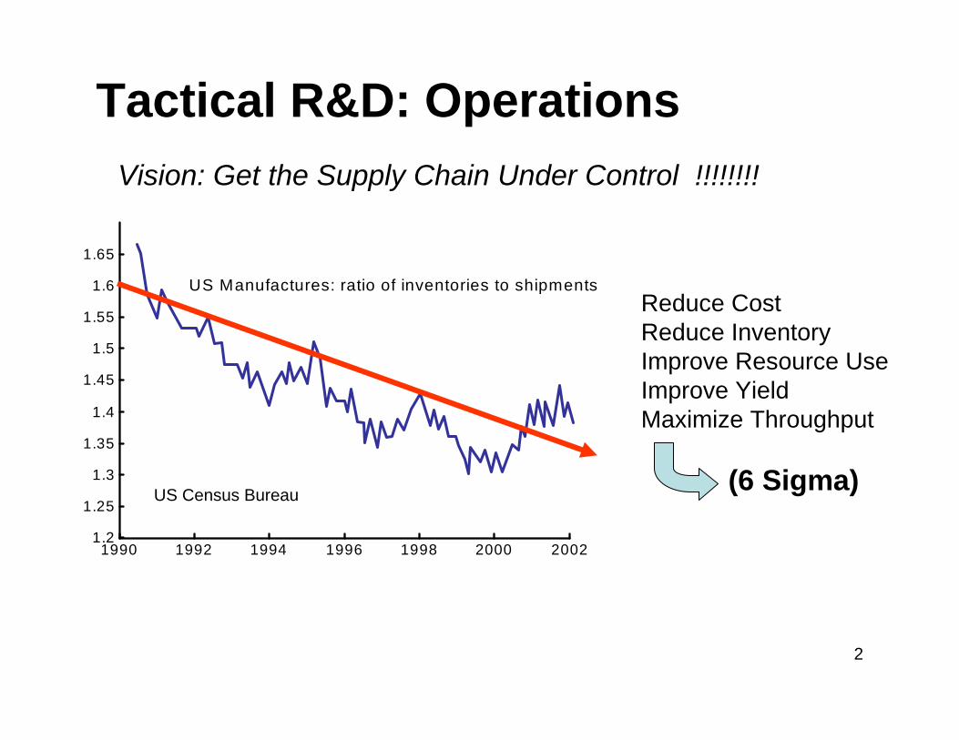
Vision: Get the Supply Chain Under Control !!!!!!!!

1990 1992 1994 1996 1998 2000 20021.2

1.25

1.3

1.35

1.4

1.45

1.5

1.55

1.6

1.65

US Manufactures: ratio of inventories to shipments

US Census Bureau

Reduce CostReduce InventoryImprove Resource UseImprove YieldMaximize Throughput

(6 Sigma)

Tactical R&D: Operations

3

1. Centralized vs Decentralized Decision Making2. Motivating examples

Supply Chain for Glass ProductionSupply Chain for Solar Cells

3. Supply Chain as a Dynamical SystemInventory controlFeedback schedulingLoad balancing and self-optimization

4. The Adaptive Enterprise 5. Current problems

Oil and gas field managementSelf-optimizing systems

6. Concluding Thoughts

4

Centralized Decision Making The chemical plant

tank

tank

mixerreactor

column

column

column

product

product

waste

supply

supply

recycle stream

5

controller

controller

controllercontroller controller

controller

controller

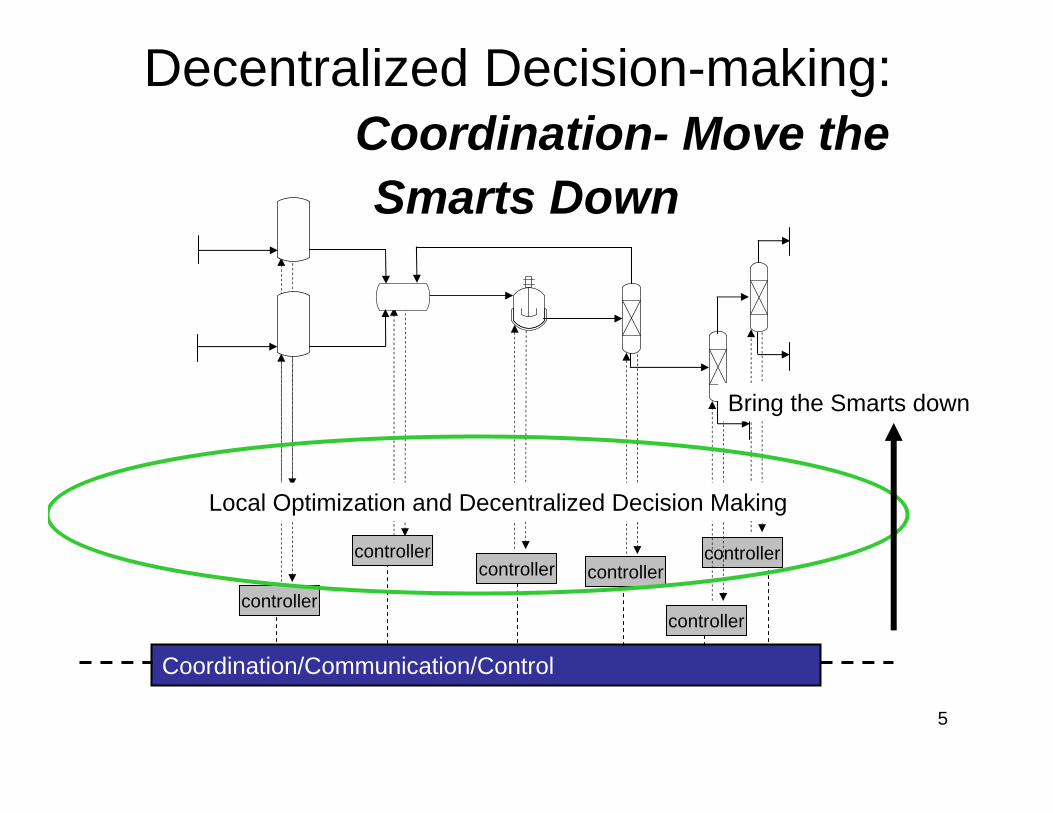
Decentralized Decision-making: Coordination- Move the Smarts Down

Coordination/Communication/Control

Local Optimization and Decentralized Decision Making

Bring the Smarts down

6

QC

Case Study 1: Windshield Manufacturwith Dr Yu JiaoPPG Inc, Glass Technology Research Center

mix melt form cool cut packSiemens/Pilkington Float Process

500 tons/day ea. line

Cut coat print form laminate packOEM discrete parts manufacturing Float Process

1000 windshields per day ea. line

QC Flat glass

windshieldsFlat glass

SandSoda-ash

+++

Center

Top

Bottom

Left

RightColor, distortion, bending depend onmix and melting conditions in furnace

10 flat glass plants

10 windshield lines

7

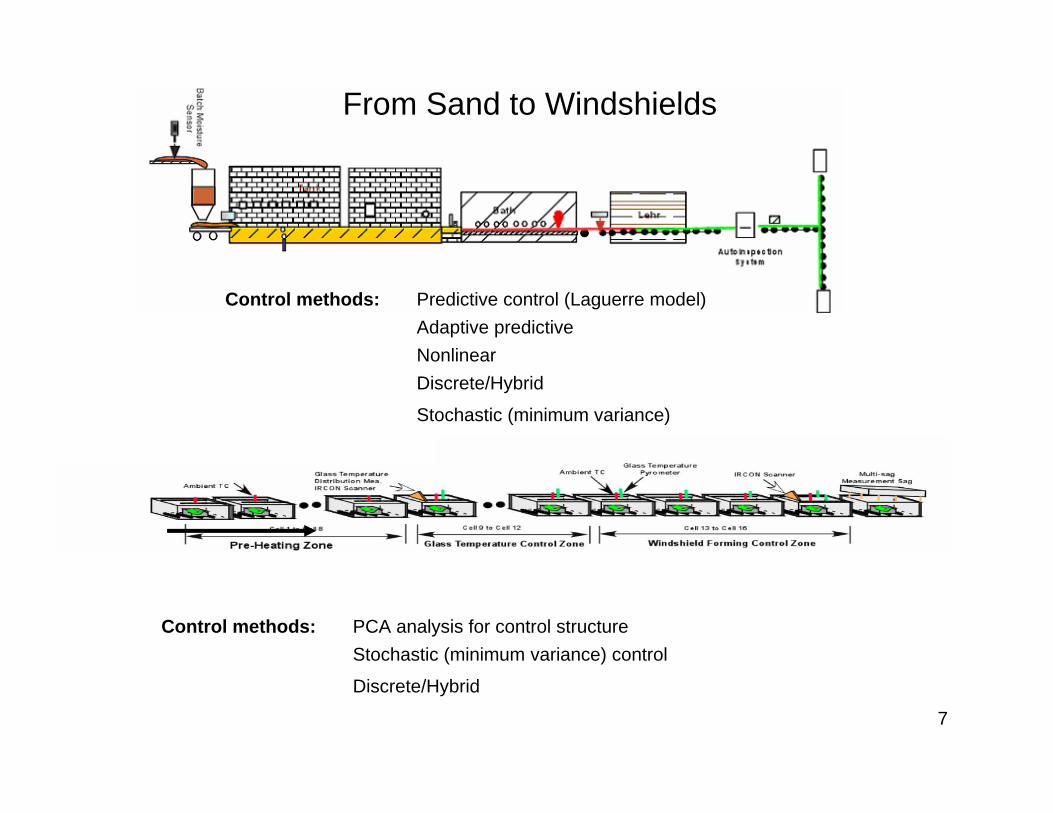
Control methods: Predictive control (Laguerre model)Adaptive predictiveNonlinearDiscrete/Hybrid

Stochastic (minimum variance)

Control methods: PCA analysis for control structureStochastic (minimum variance) control

Discrete/Hybrid

From Sand to Windshields

8

Flexible process

Vision: PPG’s supply chain will be optimized to meet market demands.

Optimal Process

Process under control

Process understandingAdvanced control(Identification,MPC,adaptation)

CFD Modeling POD reduction

Optimization atSteady state

Optimization atDuring transition

Scheduling to meet market demands

Optimized processplace new demands on control

Multi-scale models

Forecasting Marketing Sales

9

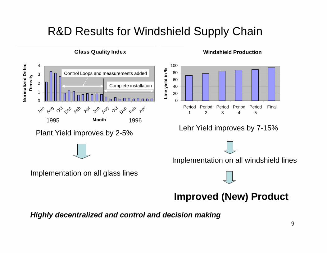
R&D Results for Windshield Supply Chain

Plant Yield improves by 2-5%

Implementation on all glass lines

Glass Quality Index

0

1

2

3

4

Jun

AugOctDec FebAprJu

nAugOctDec FebApr

Month

Nor

mal

ized

Def

ecD

ensi

ty

Series1

Control Loops and measurements added

Complete installation

1995 1996

Glass Quality Index

0

1

2

3

4

Jun

AugOctDec FebAprJu

nAugOctDec FebApr

Month

Nor

mal

ized

Def

ecD

ensi

ty

Series1

Control Loops and measurements added

Complete installation

1995 1996

Windshield Production

020406080

100

Period1

Period2

Period3

Period4

Period5

Final

Each period represents 6 mos

Line

yie

ld in

%

Series1

Lehr Yield improves by 7-15%

Implementation on all windshield lines

Improved (New) Product

Highly decentralized and control and decision making

10

Inventory Control

11

Modeling the Supply-chain

Feedback Control(optimal)

Set-point modification

Constraints:

12

The “MIT Beer Game”

Inventory

Orders

Pulse change in order level to demonstrate the Bull-Whip Effect/Demand amplification under feedback control (un-modeled delays)

Problem motivated by Paul Maurath,P&G, Cincinnati

Customerdemand

13

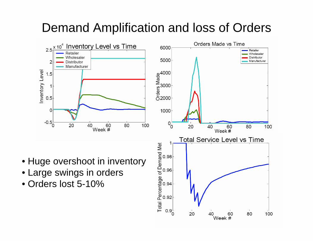
Demand Amplification and loss of Orders

• Huge overshoot in inventory• Large swings in orders• Orders lost 5-10%

14

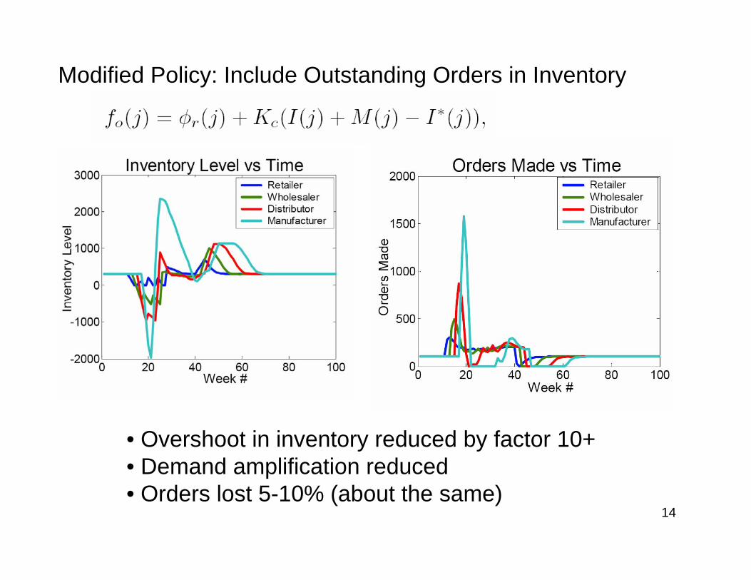
Modified Policy: Include Outstanding Orders in Inventory

• Overshoot in inventory reduced by factor 10+• Demand amplification reduced• Orders lost 5-10% (about the same)

15

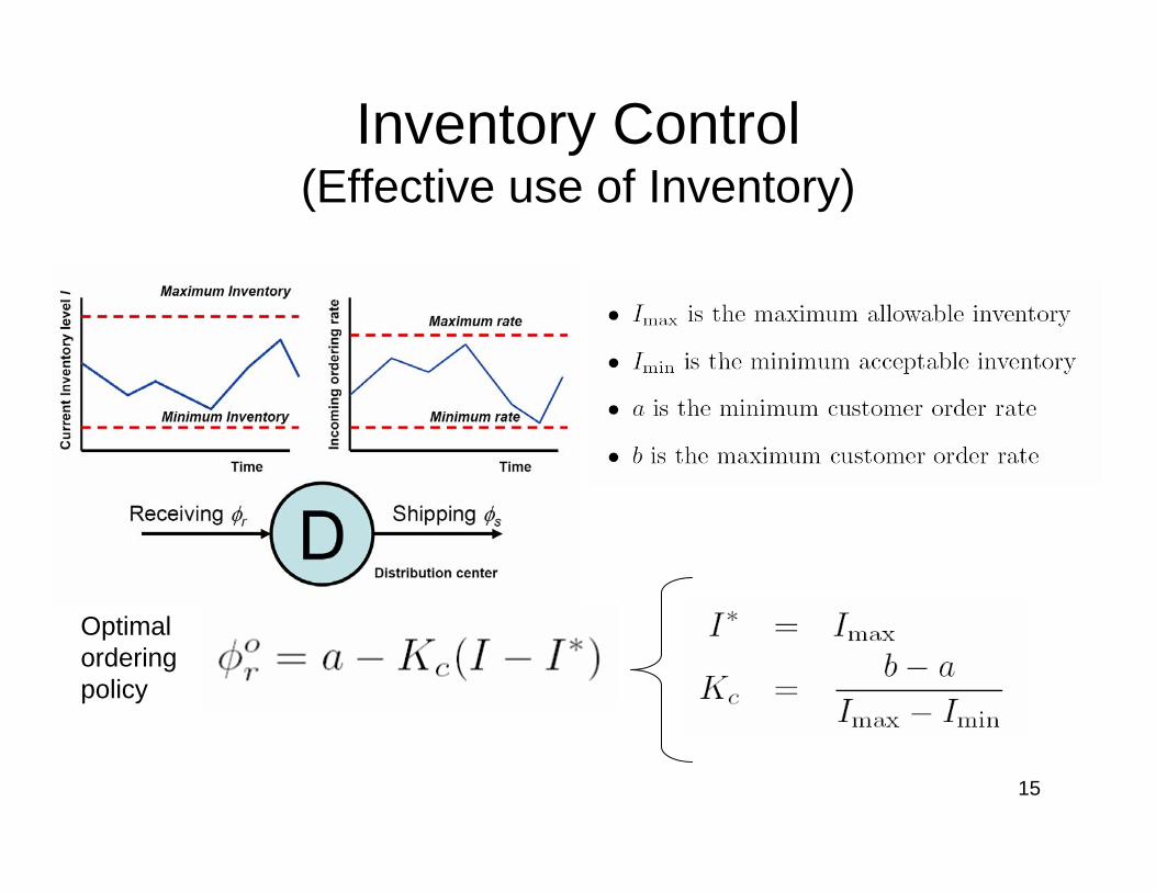
Inventory Control(Effective use of Inventory)

Optimal ordering policy

16

Optimal Storage Design for Dynamic Markets

17

Beer Game with Optimized Ordering Policy

• Inventories kept within bounds• Demand amplification eliminated• 100% service level (no lost orders)

18

Assembly, disassembly and packaging Feedback Scheduling

Operability constraint:

19

Bounds on Storage

Lower bound for storage

Upper bound for storage

20

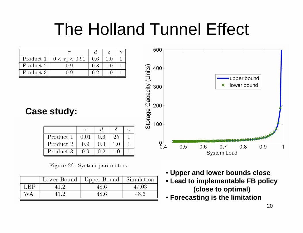
The Holland Tunnel Effect

• Upper and lower bounds close• Lead to implementable FB policy

(close to optimal)• Forecasting is the limitation

Case study:

21

Flow Control and Load Balancing

Resistor 1

Resistor 2 V1 V2

A1A2

A3

A4A5

A41

A42

A43

r1

r2

s3 = r3

s4 = r4

s5 = r5

s5s41 = r41

T3

T2

T1

r4

Maxwell’s theorem of minimum heat(Self-optimization in complex networks)

Current Law =Inventory BalanceVoltage Law= Continuity of cost

22

A1A2

A3

A4A5

A41

A42

A43

r1

r2

s3 = r3

s4 = r4

s5 = r5

s5s41 = r41

T3

T2

T1

r4

psrdtdv

+−=

0=∑Loop

iX

No value in circular activity(but there is cost)

23

Pipeline network: Simulation

atmp

INV = 0.0 m31

INV

2INV 2

OUTV

1OUTV

OUTV

valveclosed

2p

1p

valveopen

= 0.3 m380

60

40

20

00

0.05

0.10

0.15

0.20

0.25

0.30

V i[m

3 /s]

.

t [s]

Ener

gy d

issi

patio

n[k

W]

1OUTV

2OUTV

Energy dissipation

200 400 600 800

= 23.6 kW

atmp

atmp

1,21,2 1,2

IN OUTdVV V

dt= −

, , ,1 2

IN OUT IN OUT IN OUTV V V= +

Conservation laws ( .constρ = ):

Boundary conditions:

.INV const= .atmp const=,

Dynamic simulation:

24

Pipeline network: Simulation80

60

40

20

00

0.05

0.10

0.15

0.20

0.25

0.30

V i[m

3 /s]

.

t [s]

Ener

gy d

issi

patio

n[k

W]

1OUTV

2OUTV

Energy dissipation

200 400 600 800

= 23.6 kW

1,2 1,20 IN OUTV V= −

, , ,1 2

IN OUT IN OUT IN OUTV V V= +

Conservation laws ( .constρ = ):

Boundary conditions:

.INV const= .atmp const=,

min 1 1 2 2 1 1 2 2IN IN IN IN OUT OUT OUT OUTp V p V p V p VΔ + Δ + Δ + Δ

s.t.IN

i ip VΔ = iK

Hagen-Poiseuille’s law:

Optimization problem: Dynamic simulation:

25

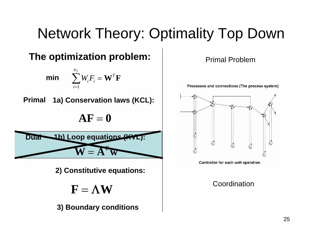
Network Theory: Optimality Top Down

=AF 0

T=W A w

1a) Conservation laws (KCL):

1b) Loop equations (KVL):

2) Constitutive equations:

=F WΛ3) Boundary conditions

The optimization problem:

1

fnT

i ii

W F=

=∑ W Fmin

Primal

Dual

Coordination

Primal Problem

26

Network Theory: Optimality Top Down

=AF 0

T=W A w

1a) Conservation laws (KCL):

1b) Loop equations (KVL):

2) Constitutive equations:

=F WΛ3) Boundary conditions

The optimization problem:

1

fnT

i ii

W F=

=∑ W Fmin

Primal

Dual

Coordination

Dual Problem

27

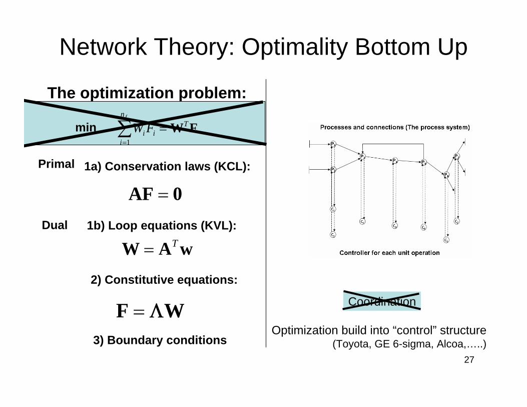
Network Theory: Optimality Bottom Up

=AF 0

T=W A w

1a) Conservation laws (KCL):

1b) Loop equations (KVL):

2) Constitutive equations:

=F WΛ3) Boundary conditions

The optimization problem:

1

fnT

i ii

W F=

=∑ W Fmin

Primal

Dual

Coordination

Optimization build into “control” structure(Toyota, GE 6-sigma, Alcoa,…..)

28

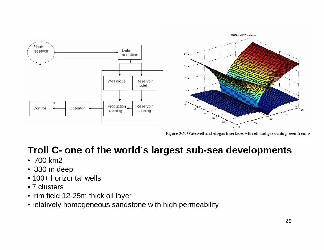
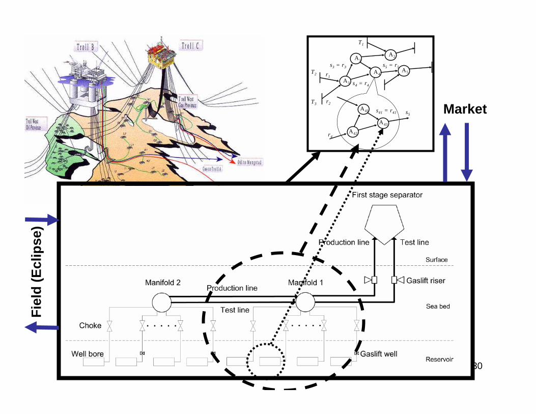
Current Research: Troll C Oil Field

IO- Center NTNU NorwayStatoil-Hydro

Objective: Maximize oil production subject to a gas rate constraint.

29

Troll C- one of the world’s largest sub-sea developments• 700 km2• 330 m deep • 100+ horizontal wells• 7 clusters• rim field 12-25m thick oil layer• relatively homogeneous sandstone with high permeability

30

Market

Fiel

d (E

clip

se)

A1A2

A3

A4A5

A41

A42

A43

r1

r2

s3 = r3

s4 = r4

s5 = r5

s5s41 = r41

T3

T2

T1

r4

31

Concluding thoughts• Tremendous opportunities in coordinating

optimization and control in real time ($50B+ in the North Sea)

• Enormous challenge (complex dynamics and large uncertainty – integration of physics computation and communication)

• Decentralized decision making (adaptive/self-optimization is required)

32

Michael’s PhD project

Complex Dynamical SystemsIntegrated in a network

Optimization A Optimization B

• Establish conditions for stability of dynamic trajectories (done)• What is the objective function being optimized?• How can the objective function be shaped by decentralized control?• How much information sharing is needed?• What is the bandwidth (response time) of the system?• Application domain TROLL C