Excitation of Helium to Rydberg States Using STIRAP A Dissertation Presented by Xiaoxu Lu to The Graduate School in Partial Fulfillment of the Requirements for the Degree of Doctor of Philosophy in Physics Stony Brook University May 2011
Transcript
Excitation of Helium to Rydberg States
Using STIRAP
A Dissertation Presented
by
Xiaoxu Lu
to
The Graduate School
in Partial Fulfillment of the Requirements
for the Degree of
Doctor of Philosophy
in
Physics
Stony Brook University
May 2011
Stony Brook University
The Graduate School
Xiaoxu Lu
We, the dissertation committee for the above candidate for the Doctor of Philosophy degree,hereby recommend acceptance of this dissertation.
Harold Metcalf – Dissertation AdvisorDistinguished Teaching Professor, Department of Physics and Astronomy
Thomas Hemmick – Chairperson of DefenseDistinguished Teaching Professor, Department of Physics and Astronomy
Xu DuAssistant Professor, Department of Physics and Astronomy
Thomas PattardSenior Assistant Editor, American Physical Society
This dissertation is accepted by the Graduate School.
Lawrence MartinDean of the Graduate School
ii
Abstract of the Dissertation
Excitation of Helium to Rydberg States UsingSTIRAP
by
Xiaoxu Lu
Doctor of Philosophy
in
Physics
Stony Brook University
2011
Driving atoms from an initial to a final state of the same parity via an interme-
diate state of opposite parity is most e!ciently done using STIRAP, because it
does not populate the intermediate state. For optical transitions this requires
appropriate pulses of light in the counter-intuitive order - first coupling the in-
termediate and final states.
We populate Rydberg states of helium (n = 12! 30) in a beam of average velocity
1070 m/s by having the atoms cross two laser beams in a tunable dc electric field.
The “red” light near ! = 790 ! 830 nm connects the 33P states to the Rydberg
states and the “blue” beam of ! = 389 nm connects the metastable 23S state
atoms emitted by our source to the 33P states. By varying the relative position
iii
of these beams we can vary both the order and the overlap encountered by the
atoms. We vary either the dc electric field and fix the “red” laser frequency or
vary the “red” laser frequency and fix the dc electric field to sweep across Stark
states of the Rydberg manifolds.
Several mm downstream of the interaction region we apply the very strong bichro-
matic force on the 23S " 23P transition at != 1083 nm. It deflects the remaining
23S atoms out of the beam and the ratio of this signal measured with STIRAP
beam on and o" provides an absolute measure of the fraction of the atoms re-
maining in the 23S state. Simple three-level models of STIRAP all predict 100%
excitation probability, but our raw measurements are typically around half of
this, and vary with both n and l of the Rydberg states selected for excitation by
the laser frequency and electric field tuning on our Stark maps. For states with
high enough Rabi frequency, after correction for the decay back to the metastable
state before the deflection, the highest e!ciencies are around 70%.
An ion detector readily detects the presence of Rydberg atoms. We believe that
the observed signals are produced by black-body ionization at a very low rate,
but su!cient to ionize about 0.5 ! 1.0 % of the atoms in a region viewed by our
detector. Many measurements provide support for this hypothesis.
5.2 Measured STIRAP e!ciencies on the manifolds of di"erent n states. . . . . . 96
6.1 Transition rates for 24S " nP and ionization rates for nP at T = 300 K . . 111
xiii
Acknowledgements
I have spent enjoyable and exciting six years at Stony Brook. This work presented in
this thesis would not have been possible without so many people’s kind help. I am heartily
thankful to everyone who has helped me in my journey and because of whom my graduate
experience has been one that I will cherish forever.
First of all, I would like to express my deep and sincere gratitude to my advisor, Prof.
Harold Metcalf. Without his inspirational guidance, I could never finish my doctoral work.
His encouragement gave me confidence to overcome every di!culty I encountered. I have
learned not only a lot of physics, but also, more importantly, the way to solve problems,
which will benefit my whole life.
I would also like to thank my colleagues for making my life as a graduate student more
enjoyable through collaboration and friendship. I want to thank Seung Hyun Lee and Andy
Vernaleken for their previous work. Without their preliminary setup, I would not know
where to start. I was lucky to have Jonathan Kaufman work together with me in the first
two years. It was a tough time for me to take over the whole experiment at the beginning,
but his passion in science and his optimism inspired me. I will never forget the days and
nights that we worked together in the lab. I would also like to thank Yuan Sun for his help in
the second half of my project. I can not imagine how I could manage to run the experiments
on my own. I am sure he is going to do a great job in keeping the experiment running and
bringing excellent results. Claire Allred and Jason Reeves have showed me great examples.
They gave me many valuable advices in both research and daily lives. Chris Corder has
helped me a lot in setting up the bichromatic beams and maintaining the blue laser system.
I also want to thank Daniel Stack and John Elgin. it was an excellent experience working
together and sharing the o!ce with them. I will miss the happy times we had together
everyday.
Many thanks are given to Dr. Marty Cohen. I am very grateful to him for the lessons,
advices, experiences he shared with me along the way. I am also thankful to him for carefully
reading and commenting on countless revisions of this thesis. It is not su!cient to express
my gratitude with only a few words. I would also like to thank Prof. Tom Bergemann for
the theoretical calculations and comments.
Among the sta" in the department, I would like to thank Pat Peiliker, Sara Lutterbie and
Linda Dixon, who helped me with all kinds of paperwork. Pete Davis has been an invaluable
source of knowledge and experience. Whenever I had a vacuum related problem, I would
turn to him for help, and he is always very patient and generous. I would also like to thank
Paul DiMatteo, Mark Jablonski, Je"rey Slechta, Je"rey Thomas and Walter Schmeling from
the machine shop. They o"ered me with their expertise in machining, and I enjoyed the
days I spent in the student machine shop to make fancy pieces for my research. Eugene
Shafto and Chuck Pancake from the electronics shop have been the ones who helped me
with expertise and knowledge in electronic circuits.
Last but not least, I want to thank my family and friends. My parents are always
supportive to my decisions, and they have taught me to be an honest and hard working
person with their own examples. I would also like to thank all my friends who have made
my life in Stony Brook a superb experience, and I will list them in my heart instead of
occupying pages of the dissertation here.
Chapter 1
Introduction
1.1 The Big Picture
Atom optics, which is a field of research exploring the possibilities of manipulating beams
of atoms in the same way that conventional optics controls light beams, has become the
subject of intense investigation in the last two decades. But the history actually started
with Stern and Gerlach’s experiments in the early 1920s [1] [2], followed by the atomic-
di"raction experiments by Estermann [3] and others in the early 1930s . These demonstrated
unambiguously that wave mechanics also applies to composite particles. These pioneering
experiments were truly di!cult to carry out due to the extremely short room-temperature
atomic de Broglie wavelength (!dB = h/Mv, where v is the velocity of atoms), of the
particles, of the order of a fraction of an Angstrom.
In the late 1970s, a renaissance in atom optics research took place when Hansch and
Schawlow proposed a method to cool atomic gases using laser radiation [4]. Experimental
and theoretical extensions of this idea eventually led to the 1997 Nobel Prize for laser-
cooling. With laser cooling, one can readily bring atomic samples down to temperatures of
1
the order of 10−6 K or less, so the atomic de Broglie wavelengths are on the order of microns
or longer [5]. The creation of the first Bose-Einstein condensates in a dilute gas of alkali
atoms [6] depended crucially on these achievements and was honored with a Nobel Prize in
2001. The new experimental tools, and the availability of widely tunable laser sources in
particular, revolutionized atom optics, and it is hardly possible to overestimate their impact
on contemporary atomic, optical, and molecular physics.
It has been shown extensively that atomic beams can be reflected [7], di"racted [8][9]
and focussed [10][11][12][13], with laser beams tuned around atomic resonances. Besides
using light (oscillating electric field) to steer atoms, one can also achieve useful focusing by
adding a static electric field (or magnetic field) gradient on a beam of slow neutral atoms
[14]. This focussing force arises from the interaction of the electric field gradient with the
induced electric dipole moment of the atom. Kalnins et. al. [15] have used an electrostatic
lens with three focusing elements in an alternating-gradient configuration to focus a fountain
of cesium atoms in their ground state. Because no external magnetic fields are introduced,
electric field gradient focusing is suitable for magnetic-field sensitive experiments such as
atomic fountain clocks and electron electric dipole moment experiments.
Ground state neutral atoms are not a"ected greatly by electric fields as they don’t have
large electric dipole moments, so huge electric field amplitudes and long acceleration times
are needed to get e"ective focusing, as in [15]. However, by exciting neutral atoms to high
Rydberg states, their electric dipole moments are increased considerably. The goal of our
work was to demonstrate the focusing e"ect of an inhomogeneous electrostatic field on neutral
atoms by manipulating the trajectories of the Rydberg atoms. Although the original idea
for this focussing was first introduced in 1981 [16], it took rather long time to develop the
proper experimental techniques to realize it. In this thesis, we concentrate on the su!cient
production of Rydberg atoms in helium via the STIRAP technique.
2
In our experiments, we excite He atoms to Rydberg States (n = 12 ! 30) from a
metastable (23S1) atomic beam (He*). The atoms in the beam cross two laser beams in
a tunable dc electric field. The “red” light near ! = 790 ! 830 nm connects the 33P states
to the Rydberg states and the “blue” beam of ! = 389 nm connects the metastable 23S
state atoms emitted by our source to the 33P states. By varying the relative position of
these beams we can vary both the order and the beam overlap encountered by the atoms.
This two-step process allows a very high excitation e!ciency when the atoms encounter the
sequence of light pulses that corresponds to Stimulated Rapid Adiabatic Passage (STIRAP)
[17][18].
Our interests in highly e!cient production of Rydberg atoms stems from the use of
inhomogeneous electrostatic fields to control atomic motion for use in atomic optics, but
STIRAP itself is a very interesting and broad topic, and is a powerful way to coherently
transfer population in a three-level system. Ideally, in the adiabatic limit almost 100% of the
population can be transferred to the target state, whether in a # scheme, $ scheme or ladder
scheme. It is not sensitive to moderate changes in pulse parameters such as pulse length,
amplitude, or intermediate detuning (as along as two-photon resonance condition is satisfied).
E!cient population transfer using STIRAP has been demonstrated experimentally as well
[19] [20][21], but mostly in low-lying states. STIRAP excitation to high Rydberg states is also
possible, but di!cult due to the low oscillator strength of optical Rydberg transitions [22].
To better understand the STIRAP process, we want to investigate extensively the STIRAP
excitation to di"erent Rydberg states and measure the absolute e!ciency of excitation.
One of the possible applications of this atom optic technique is neutral atom nanolithog-
raphy [23]. The high internal energy of He* atoms could be exploited to create nanoscale
structure through a resist assisted lithography mode [24]. Preliminary results showing the
focusing e"ect of an electric hexapole lens on Rydberg atoms have been described in S-H.
3
Lee’s thesis [25].
1.2 Rydberg Atoms
1.2.1 General Properties
Rydberg atoms are excited atoms with one or more electrons that have a very high
principal quantum number [26]. Rydberg states of atoms have been attracting the interest
of atomic physicists for more than one century. At the end of the 19th century, Balmer
related a series of spectral lines of atomic hydrogen to the famous formula named after him
[26]
! =bn2
n2 % 4(1.1)
with b = 3645.6 A. It became clear that the series related energy di"erences between n =
2 and high energy states after Hartley [27] expressed Balmer’s formula in terms of wave
numbers instead of wavelength:
# = (1
4b)(1
4% 1
n2) (1.2)
High lying states are called Rydberg states because Rydberg was able to express the wavenum-
bers of di"erent series of alkali atoms [28] with a single formula
#l = #∞l %Ry
(n% $l)2(1.3)
where #∞l is the series limit, $l is the quantum defect and Ry = 109721.6 cm−1 is the universal
Rydberg constant. Another great achievement of Rydberg was the discovery that the lines
connecting series can be obtained by setting #∞l = Ry/(n′%$l)2. The physical meaning of the
principal quantum number n and the Rydberg constant became clear after Bohr proposed
4
his model for the hydrogen atom in 1913. Then Ry could be written as
Ry =Z2e4me
2(4"%0!)2= Z2mc2&2
2(1.4)
where %0 is the permittivity of free space, ! is the Planck’s constant, Z is the proton number,
e is the electron charge and me is the electron mass.
Rydberg atoms can be generated by charge exchange or electron impact [26]. When a
positive ion collides with a ground state atom, the ion captures one electron from the ground
state atom and is left in a Rydberg state. If an electron beam hits ground state atoms,
it could also possibly excite them to Rydberg states. Optical excitation became feasible
with the advent of lasers. The big advantage of optical excitation over charge exchange
and electron impact excitation is that individual Rydberg states can be accurately accessed
through tuning of the photon energy.
These Rydberg atoms have a number of peculiar properties so that some of the e"ects
impossible to detect in ground state atoms become obvious in Rydberg atoms. As listed in
Table 1.1, the orbit radius of Rydberg atoms is much larger, & n2. As a consequence, Ryd-
berg atoms have very large dipole moments and polarizabilities which lead to a pronounced
Stark e"ect [29] and van der Waals interaction between pairs of Rydberg atoms [30][31].
Neighboring states with di"erent principal quantum numbers are close so that transition
between Rydberg states can be driven by microwaves. Furthermore, Rydberg atoms are
particularly sensitive to their local environment. Ambient blackbody radiation redistributes
Rydberg atoms between neighbouring energy states and even leads to ionization and could
significantly shorten the total lifetime of the Rydberg state. And with the production of
cold Rydberg atoms, there has been renewed interest in low temperature Rydberg systems
for applications such as studies of collective e"ects [32] and formation and recombination of
5
Property Formula n-dependence
Binding energy En % Ry
(n−!l)2n−2
Energy spacing En % En−1 n−3
Orbital radius 'r( ) 12(3(n% $l)2 % l(l + 1)) n2
Geo. cross section "'r(2 n4
Dipole moment 'nl|er|nl + 1( n2
Polarizability 2e2!
n=n!,l,m|〈nlm|z|n!l!m!〉|2Enlm−En!l!m!
n7
Radiative lifetime ( e2
3!c3"#0
!l=l±1n<n!
lmax2l!+1'
3|'n′l′|r|nl(|2)−1 n−3
Blackbody transition 1$bbnl
= 4%3kT3n2 n−2
Fine Structure n−3
Table 1.1: Selected properties of Rydberg atoms and their dependence on the principalquantum number [26].
ultracold Rydberg plasmas [33] and quantum computing [34]. In the following sections of
this chapter, I am going to focus only on the important properties related to our experiments,
the quantum defect and Stark e"ect on helium Rydberg states.
1.2.2 Quantum Defects
The energy levels of hydrogen can be easily calculated from the Schrodinger equation.
These levels turn out to be only dependent on the principal quantum number n, En = %Ry
n2 ,
such that di"erent l states are degenerate. In non-hydrogen atoms, the excited valence
electron in a Rydberg state does not only interact with the nucleus but also with the core
electrons. When the valence electron is far away from the nucleus, the many core electrons
provide e"ective shielding from the electric field of the nucleus, so that the outer electron
6
generally “sees” a nucleus with only one proton and will behave much like the electron of a
hydrogen atom. However, if orbits of electrons pass through the core of shielding electrons,
then the electron will occasionally “see” the whole nucleus. Then the energy levels of non-
hydrogen atoms will be depressed with respect to their hydrogen counterparts, and can be
written as [35]
En = % Ry
(n% $l)2(1.5)
where the quantum defect $l in general is a function of n and can be described by the
Rydberg-Ritz formula [36]
$l = a+ bEn + cE2n + dE3
n + ... (1.6)
where a, b, c, d,... are the Rydberg-Ritz coe!cients and depend on the angular momentum
l. Their values for triplet helium atoms are listed in Table 1.2. With low angular momentum
states, the shielding e"ect breaks down a bit and the electron energy levels can not mimic
those of hydrogen without the shielding, hence the quantum defect is higher. For S states, the
quantum defect is relatively large since electrons with zero angular momentum essentially
pass cleanly through the core of shielding electrons. For D states, having higher angular
momentum, the quantum defect is a lot smaller, as their orbits will not pass through the
core so deeply. Furthermore, even though the high - l Rydberg electrons do not penetrate
the core, they do polarize it, and this also leads to non-zero quantum defects [37].
1.2.3 Stark E"ect in Helium Atoms
Because the helium Rydberg states are hydrogenlike in many aspects, let’s first look at
the Stark structure of hydrogen. The Schrodinger equation in atomic units (! = e = m = 1)
7
l - value a b c d
0 0.296609 -0.038840 0.004960 0.000000
1 0.068320 0.017870 -0.017190 0.000000
2 0.002869 0.006220 0.000000 0.000000
3 0.000240 -0.002090 0.000000 0.000000
Table 1.2: Rydberg-Ritz coe!cients for the calculation of quantum defect of triplet Heliumwithout considering spin-orbit splitting [38]
for the hydrogen atom in an external field is
(%1
2*2 % 1/r + Fz)$(%"r ) = W$(%"r ) (1.7)
W is the energy and F is the magnitude of the electric field in atomic units, 5 + 1011V/m,
which is taken to lie along the z axis. Eqn. 1.7 may be separated in parabolic coordinates
and can be solved analytically for zero electric field [26]. If the electric field is not zero,
perturbation theory can be applied to evaluate the perturbed energies and the results are
given as
W0 = %1/2n2
W1 =32n(n1 % n2)F
W2 = % 116n
4[17n2 % 3(n1 % n2)2 % 9m2 + 19]F 2
(1.8)
where the quantum numbers n and m label the principal and magnetic quantum numbers
respectively, and n1, n2 are non-negative integers obeying
n1 + n2 + |m|+ 1 = n (1.9)
8
For atoms other than hydrogen, there are important di"erences due to the presence of
the finite sized ionic core. The wavefunction is no longer separable in parabolic coordinates.
The single-electron Hamiltonian in an external electric field reads
H = H0 + Fz +Hfs (1.10)
where H0 is the unperturbed Hamiltonian and Hfs is the energy shift due to fine structure
which is small in high n states of He and can be neglected. We are interested in the energies
of the Stark states as a function of field strength, the so called Stark map. To calculate the
eigenvalues of (1.10), we represent the Hamiltonian in the basis provided by the eigenvector
|nlm( of the field free Hamiltonian in a spherical basis. As the eigenvalues of the field-free
Hamiltonian are known, we only have to evaluate the o"-diagonal matrix elements
'nlm|Fz|n′l′m′( = F 'nlm|r cos (|n′l′m′( (1.11)
= $(m,m′)$(l, l′ ± 1)F 'lm| cos (|l′m′('nl|r|n′l′( (1.12)
The angular part of the matrix elements has well-known analytic solutions in a spherical
basis. We can numerically evaluate the radial matrix elements of the Stark operator as
described by Zimmerman et al.[29].
The resulting energy levels for He n= 26 are shown in Figure 1.1. The figure demonstrates
several important properties: (1) the strong suppression of the s, p, d states due to their
quantum defects; (2) the lifting of the zero-field degeneracy of the |nl(, l > 3 states; (3)
avoided crossings of appreciable size. Avoided crossings arise from the fact that a non-
hydrogen core breaks the Coulomb symmetry and couples the Stark levels. The size of an
avoided crossing is given by the strength of the coupling.
9
Figure 1.1: Stark Structure of Helium atom for n = 26 (without considering the fine struc-ture) [38]
With an applied electric field, all the di"erent l levels are mixed and l is not a good
quantum number any more. We usually call the region with mixing l states the manifold,
while the S states at low electric field are well separated and easily distinguished.
Meanwhile, at di"erent electric fields, di"erent Stark states have di"erent oscillator
strengths for transitions to other states. The oscillator strength from level nlm to level
n′l′m′ is defined by
fn!l!m!,nlm = 2m
! 'n!l!,nl|'n′l′m′|z|nlm(|2 (1.13)
For He Rydberg Stark states, these oscillator strengths can only be calculated by numerical
10
Figure 1.2: Relative Transition strength to n = 26 Stark map from 33P2 for triplet Heliumatom, which is given by the width of each line [38].
integration. The resulting transition intensity of the excitation of n = 26 Stark states from
the 33P2 state is shown in figure 1.2 [38]. This is qualitatively applicable to other n states.
At zero field, the S and D states are directly dipole coupled to the P state, resulting in
large transition probabilities. By increasing the electric field, there are dramatic changes in
the distribution of the oscillator strength across the Stark manifold. The minimum near the
center (! 163 cm−1) was attributed to the S %D interference of the transition momentum
between the 33P and final Stark states [39]. Before reaching the anti-crossing region, the
coupling between the S state and other manifold states is very small due to the quantum
defect, so the transition strength does not change much. These di"erent transition strengths
will lead to di"erent Rabi frequencies and also di"erent lifetimes.
11
1.3 Excitation of Helium to Rydberg States
The atomic energy level scheme for He is shown in Figure 1.3. He is a closed shell system
like all rare gases. When one s-electron is excited from the core to a high lying metastable
state, the atom behaves e"ectively like a single electron atom. However, metastable helium
(He*) does not have a closed inner shell like alkali metals, but an open S-state core. The
coupling between the core and excited electron spins results in either spin-opposed (singlet)
or spin-parallel (triplet) states, causing the splitting within the triplet P states shown in
Figure 1.3. However, the level structure is simplified by the fact that there is no nuclear
spin, so there is no hyperfine structure.
Neither the singlet nor triplet S states can decay to the ground 11S0 state via an electric
dipole transition due to the %L = ± 1 selection rule (L being the orbital angular momentum
quantum number which is zero for S states). Consequently the singlet and triplet S states
are metastable, with the 21S0 state having a lifetime of ! 19 ms. However, decay of the 23S1
state is doubly forbidden because a transition to the ground state also requires that one of the
electron spins has to flip to create a ground singlet state. This gives rise to the extremely long
metastable lifetime, predicted to be 8000 s [40], so that the metastable state can essentially
be regarded as the e"ective ground state. The He* 23S1 state is the longest lived of any
atomic or molecular species and decays via a single-photon magnetic dipole transition at
62.5 nm rather than via a two-photon process [41]. Meanwhile, the stored metastable energy
(19.82 eV) is the highest for any metastable species, enabling detection of single atoms using
charged particle detectors, electron multipliers, or microchannel plates (MCPs) with near
unity detection e!ciency [42]. Similarly, the large stored energy in He* allows for e!cient
damage of photoresist-coated surfaces for applications in atom lithography.
Since we can not excite the ground state He to metastable states by any optical transition,
12
792 – 830 nm
(a) (b)
Figure 1.3: Energy level diagram for the triplet states of Helium (a) and the transitionscheme to the Rydberg states (b). &S and &P are the Rabi frequencies of the Stokes andthe Pump lasers, respectively. %S and %P are their detunings, which will be discussed inmore detail in Chapter 4.
13
as a first step of excitation, the He* atoms are produced in a reverse flow dc discharge
source. The source output is about 1014 He* atoms/sr·s, a few parts in 106 of the total He
flux. The ground state atoms are e"ectively lost as they cannot be detected and collisions of
He* on ground state He have negligible e"ect on the populations. Chapter 2 gives a detailed
description of the source, as well as the interaction region and the available detection systems
in the vacuum system.
The three-level excitation scheme used in this experiment is illustrated in Figure 1.3(b).
After the dc discharge brings 10−5 of the total He atoms to the 23S1 metastable state,
a frequency-doubled Ti:Sapphire laser of ! = 389 nm (“blue”) connects the metastable
23S1 state (|1() atoms emitted by our source to the 33P2 (|2() state. Another independent
Ti:Sapphire laser, which could be adjusted in its wavelength from 780 ! 830 nm (“red”)
is used to drive the excitation from the intermediate state 33P2 to selected Rydberg states
(|3(). We always keep the “blue” light locked on |1( " |2( resonance, and then, either vary
the dc electric field and fix the “red” laser frequency or vary the “red” laser frequency and
fix the dc electric field to sweep across the Stark states of the Rydberg manifolds. Details
of the laser systems will be covered in Chapter 3.
The short lifetime of the intermediate 33P2 state (! 94.8 ns [5]) introduces the main
loss during the excitation process due to its spontaneous emission to 23S1 and 33S1 states.
Instead of doing the excitation in the intuitive order, we employ the Stimulated Raman
Adiabatic Passage (STIRAP) technique by first coupling the intermediate and final states,
which allows us to achieve much higher transfer e!ciency, as will be described in detail in
Chapter 4.
The third laser at != 1083 nm coupling the 23S1 and 23P2 states is not used for excitation,
but as a tool to separate the remaining metastable He* from the other Rydberg state atoms
for excitation rate measurements. Several mm downstream of the interaction region, we
14
apply the very strong bichromatic force [43] on the 23S1 " 23P2 transition. It deflects the
remaining 23S1 atoms out of the beam and the ratio of this signal measured with the STIRAP
beams on and o" provides an absolute measure of the fraction of the atoms remaining in
the 23S1 state. The setup of absolute e!ciency measurement followed by the experimental
results will be discussed in Chapter 5.
After He atoms are excited to Rydberg states, they are easily ionized and then collected by
our ion detector. We believe that the observed signals are produced by black-body ionization
at a very low rate, but su!cient to ionize about 0.5 ! 1 % of the atoms in a region viewed by
our detector. Many measurements provide support for this hypothesis. Details are provided
in Chapter 6 followed by a summary and outlook in Chapter 7.
15
Chapter 2
Vacuum System
In earlier experiments, we used an old vacuum system pumped by three di"usion pumps
backed by two big mechanical pumps, which has been described very well in S-H. Lee’s
and A. Vernaleken’s theses [25][44]. But that vacuum system was all O-ring sealed and it
leaked here and there from time to time. And with some oil contamination, the pressure was
about ! 10−5 Torr in the source chamber, ! 2 + 10−6 Torr in the interaction chamber and
! 8 + 10−7 Torr in the detection chamber, and not very stable. When the booster pump
finally stopped working, we started to take apart the old vacuum system and build a new one
in early 2007. Here, I am just going to talk about the new system in which my experiments
were done.
2.1 The Whole System
The vacuum system is primarily made of stainless steel with conflat flanges sealed with
copper gaskets. It consists of three main parts: the source chamber where the metastable
helium atoms are created, the interaction chamber where we do STIRAP to excite the atoms
16
to the Rydberg states and the detection chamber where the atomic distribution is measured
after a long beam line. The layout of the system is shown in Figure 2.1.
The source chamber and the interaction chamber are separated by a wall with a 5 mm
aperture so that they are di"erentially pumped. The source chamber is pumped by a Pfei"er
TPH330 Turbo pump (330 L/s) backed by a Welch Duo-Seal mechanical pump 1397 and
the source outlet is pumped by a Welch Duo-seal pump 1402. The interaction chamber is
pumped by a Pfei"er TPH 270 Turbo pump (270 L/s) with a Welch 1376 mechanical pump
acting as a backing pump. The bellows between the chambers and Turbo pumps serve as
vibration dampers. Although the TPH330 Turbo only pumps the source chamber, which
is a much smaller volume, it has to handle the large influx of helium gas when the source
is running (as described in the following section). During operation, the detection chamber
and the interaction chamber are usually connected, but we have another ion pump on the
detection chamber, so the detection chamber pressure is typically a little lower. Typical
pressure in our vacuum system (without gas flow to the source) is 3.2 + 10−7 Torr in the
source chamber, 3.6 + 10−7 Torr in the interaction chamber and 2.5 + 10−7 Torr in the
detection chamber. With source running, the pressure in the interaction chamber is about
10−6 Torr.
The vacuum system is constructed such that the chambers can be vented to atmosphere
pressure with the Turbo pumps on. In order to do so, the two six inch O-ring sealed
gate valves inserted between the chamber and turbo pumps in the source region and the
interaction region are closed. Afterwards, when we want to return to high vacuum, we close
the foreline valves FS and IS in Figure 2.1, and open the roughing valves RS and RI. It
takes a few minutes to pump the chamber below 100 mTorr, then we close the RS and RI,
open FS, IS and two gate valves to let the Turbo pumps work on the chambers as usual.
An additional gate valve isolates the detection chamber from the rest of the vacuum system
17
Vacuum!system
slits
26cm
roughing!line
foreline
foreline
roughing!line
Welch!Duo!1397 Welch!Duo!1376
Interaction!chamber
Detection!chamber
Gate!valve
Gate!valve
Gate!valve
RS!valve
FS!valve
RI!valve
RI!valve
Safety!valve Safety!
valve
Welch!Duo!1402
140cm
Vibration!damper
Vibration!damper
TPH!270
TPH!330
Liquid!N2reservoir
Figure 2.1: Vacuum system layout. It has three main chambers: source chamber, interactionchamber and detection chamber
18
and the detection chamber can be roughly pumped by two cryogenic sorption pumps with
molecular sieve material inside.
To prevent oil from back-streaming into the system from mechanical pumps in an emer-
gency, such as power outage, we put pneumatic safety valves on all three mechanical pumps.
The valves remain open if power is on and the pressure on the mechanical pumps side is
lower than the foreline side. If the power is o" or something is wrong with the mechanical
pumps, the valves would shut themselves o" immediately so that the mechanical pumps are
isolated from the rest of the system. For further protection from oil contamination, we have
coaxial copper sieve foreline traps on both Turbo backing pipes.
2.2 Source Chamber
Since the energy gap between the 23S1 and the 11S1 state is about 19.8 eV and the
transition itself is doubly forbidden, we can not excite the ground state He to the metastable
state by any optical transition. Instead a metastable helium beam is created by a dc discharge
in moderate pressure He gas. The gas then freely expands to a lower pressure region through
a small aperture.
The source we are using is based on the reverse flow design developed by Kawanaka et al.
[45], slightly modified by Mastwijk et al. [46], and fabricated at Utrecht University in the
Netherlands. It was first assembled in July 2007 and started to produce a stable metastable
helium beam in Oct. 2007.
As shown in Figure 2.2, there is a 1 cm diameter pyrex glass in the center, held by a
Teflon piece at the narrow end and by an O-ring at the other end, inside a 3 cm stainless
steel coaxial jacket which is cooled by liquid nitrogen to 77 K. Helium gas flows into the
chamber between the gas tube and the cooled jacket. The Teflon spacer further narrows
19
Figure 2.2: Metastable helium source with the reverse flow design [47]
20
the spacing and enhances the contact between the helium atoms and cold wall, so that the
atoms are considerably cold when they reach the tip of the glass tube, i.e. the discharge
region. Then most of the atoms are pumped out through the glass tube by the Welch 1402
mechanical pump. Inside the glass tube, there is a 1 mm diameter tungsten rod with one
end sharpened to a needle-like point, centered in place by a ceramic spacer. The spacer has
several channels cut into it to allow appropriate flow of helium gas. At the end of the steel
jacket housing, in front of the glass tube, a piece of aluminum plate with a 0.5 mm aperture
serves as a nozzle plate. The tungsten needle is mounted on a linear motion feedthrough
(range of motion: 1 inch) so that we can adjust the distance between the tip of the needle
and the nozzle plate. The Tungsten needle and the nozzle serve as cathode and anode for
the dc discharge, respectively. To start the discharge source, %2200 V are supplied to the
needle while the nozzle plate is held at ground potential.
In the high field region, the background gas gets field ionized and forms a discharge plasma
consisting of He ions, metastable He (He*) and other excited states of He. Unfortunately,
most of the metastable atoms are quenched by collisions in the high pressure dense region.
But outside the discharge region, after the nozzle plate, the density is lower and collisions are
less likely. Therefore, a fraction of the He atoms are excited again to the metastable state
by collisions with secondary electrons. Overall, the metastable state only makes up a small
fraction (10−4 ! 10−5) of the total number of He atoms in the beam. After the nozzle plate,
there is a 3 mm aperture, called a skimmer plate, attached to the wall separating the source
chamber and the interaction chamber. The metastable He atoms fly through the skimmer
plate into the interaction chamber together with charged particles, visible light, UV light
and ground state He. To allow for alignment of the nozzle aperture to the skimmer aperture,
the source is attached to the chamber by a bellows piece.
To make the He* source work properly, the following parameters must be optimized,
21
mostly by trial and error. Flow pressure, distance from the needle to the nozzle plate, and
the discharge current are all important. It was found that the cleanliness of the glass tube,
the sharpness of the tungsten needle, whether the needle is centered inside the glass tube,
and the quality of the nozzle plate surface are also important.
In our setup, we have a needle valve in the He inlet line to control the flow. However,
we measure the outlet pressure instead of the inlet pressure by a digital Granville-Phillips
Convectron gauge. The source could run steadily from about 1.8 Torr to 4 Torr. But higher
outlet pressure leads to fewer metastable He atoms. The absolute amount of helium atoms
at 4 Torr is only about 55% of what it is at 2 Torr (see Figure 5.10). Running at lower
pressures also causes the discharge to become unstable. To get a stable intense metastable
beam, we usually run the source at about 2.2 Torr.
A high voltage on the needle tip is required to create a high electric field to start the
source. But the higher the current, the higher is the velocity of the He* in the beam. Since
running the discharge at high currents dramatically shortens the source lifetime, we run our
source in a current limiting mode. We put a 100 M& power resistor in series with the source
circuit. Although the discharge could run from about 2.5 mA to 12 mA, we typically run
the source at about 7 ! 8 mA with %2200 V at the needle as a trade-o" among metastable
productivity, longitudinal velocity and source lifetime.
Sometimes, if the source doesn’t start immediately after we turn on the voltage, we
might need to adjust the needle position slightly. As long as the source is lit, the needle
position doesn’t matter that much. We have a 2-3/4” Conflat window around the skimmer
plate region so that we can see if the source if working properly or not. When it is working
correctly, the source glows a blueish color and is very bright. If there is only a very weak
yellow spot around the skimmer aperture, there is probably a discharge inside the glass tube.
And occasionally, when the glow is much dimmer, it is just not the right state of discharge.
22
With source gas flowing, the pressures in the source and the interaction chamber are
about 10−5 Torr and 10−6 Torr respectively as measured by ion gauge respectively. The
source turbo pump backing pressure reads about 100 mTorr and the interaction chamber
turbo pump backing pressure rises up to 50 mTorr. Under steady running conditions, our
source yields ! 0.5+ 1014 He* atoms/(sr·s) with a average longitudinal velocity about 1070
m/s and full width at half maximum of about 480 m/s.
2.2.1 Time of Flight Measurement
The longitudinal velocity distribution of the atomic beam was characterized by a time-
of-flight (TOF) measurement. A mechanical chopper was put in the interaction region with
a linear motion feedthrough. Then we used the SSD detector as described in Section 2.4.2 to
detect the beam about 1.4 meters downstream in the detection region. Measuring the arrival
times of the light and atoms yields the longitudinal velocity distribution of the atomic beam.
The chopper moves a resonant frequency of about 175.9 Hz with a small slit about 300
microns wide glued on it. Figure 2.3 shows a typical signal of the TOF measurement.
The first peak corresponds to UV photons from the source discharge and the second peak
originates from the metastable atoms. The delay time from the first peak is the time it
takes for the atoms to travel from the chopper to the detector. So from the curve, we get an
average longitudinal velocity of 1070 m/s and velocity spread of about ±240 m/s. The data
was taken with flow pressure at about 1.8 Torr and needle voltage of 2.3 kV voltage with 8
mA current.
23
0.0 0.5 1.0 1.5 2.0 2.5
0
20
40
60
80
100
SSD signal (mV)
Time (ms)
Vlongitudinal
= 1070 240 m/s
Figure 2.3: Longitudinal velocity distribution of He* atoms determined in a time-of-flight(TOF) measurement
2.3 Interaction Chamber
The atoms entering the interaction region are collimated by the slits about 23 cm down-
stream from the skimmer plate. A horizontal slit about 0.3 mm wide is mounted on a
vertical motion feedthrough and a vertical slit about 0.5 mm high is mounted on a hori-
zontal feedthrough so that we can independently move the slits vertically and horizontally .
Then, at an additional 5 cm downstream before the interaction chamber, we have another
round stainless steel plate with a 2 cm diameter hole in the center, making good contact
with the inside wall, to block all other particles flying around in the chamber.
Figure 2.4(a) shows the inside of the interaction chamber. Two electric field plates made
of brass whose dimensions are shown in Figure 2.4(b) are located at the center of the chamber
with their short side aligned approximately parallel to the atomic beam. On both sides of
the interaction chamber, we have 4.5” diameter windows on 6” conflat flanges, antireflection
24
Figure 2.4: Interaction region : (a) configuration of atomic beam, laser beams, field platesand electrostatic lens (b) dimension of field plates [25]
coated for 389 nm, 796 nm and 1083 nm. Thus our laser beams used for the STIRAP
excitation process and the detection process can enter the chamber perpendicularly to the
atomic beam with less than 1% reflection loss. A few 2-3/4” flanges with BNC feedthroughs,
with 0.094 inch diameter pins on the vacuum side, are mounted on the chamber. The voltages
for field plates and ion detector are supplied by single-strand Kapton wires (from MDC,
diameter: 0.61 mm) and push-on connectors connected to the pins on the feedthroughs.
2.3.1 Ion Detector
The ion detector for ionized Rydberg atom detection is placed in the interaction chamber.
It sits close to the downstream edge of the upper field plate supported by insulated screws
25
‐50 V
‐800 V
‐1600 V
‘
Figure 2.5: Ion detector schematic
to monitor the ionized Rydberg atoms produced during the experiment. The ion detector
includes two microchannel plates (MCP) in the Chevron configuration as shown in Figure
2.5.
The microchannel plate consists of thousands of very thin, tiny conductive glass cap-
illaries (microchannels) fused together and sliced into a thin plate. Each microchannel is
a continuous dynode electron multiplier, in which the multiplication takes place under the
presence of a strong electric field. A particle or photon that enters one of the channels
through a small orifice is guaranteed to hit the wall of the channel due to the channel being
at an angle to the plate. The incident particle frees an electron from the channel wall. Then,
with an electron-accelerating potential di"erence applied across the length of the channel,
the initial electron strikes the adjacent wall, freeing several electrons via “secondary emis-
sion”. These electrons will be accelerated along the channel until they in turn strike the
channel surface, giving rise to more electrons. Eventually this cascade process amplifies the
26
original signal by several orders of magnitude depending on the electric field strength and
the geometry of the microchannel plate. There is a nice review article of MCPs by Wiza
[48].
The MCPs in use were purchased from Burle Electro-Optics. The Channel diameters are
10 microns with a center to center spacing of 12 microns. They have a bias angle of 12 and
a length to diameter ratio of 40:1. The gain of the MCPs is about 103 at 750 V bias voltage
and 2+ 103 at 800 V. As shown on Figure 2.5, an acceleration voltage of %1600 V attracts
ions created from Rydberg atoms to the first MCP, where they are amplified twice (total
gain about 2 + 106), then a metal anode after the second MCP collects the electrons. The
resulting current is converted to voltage signal that can be observed with an oscilloscope if
there is any Rydberg production during scanning the electric field or the red light frequency.
2.4 Detection Chamber
2.4.1 Phosphor Screen Detector
The basic principle of our MCP/Phosphor Imaging Detectors is a conversion of initial ra-
diation into an “electron image”, which is amplified by microchannel plates, then converted
to a visible image registered by a CCD camera. Our metastable helium atoms incident on
the MCP produce an electron shower due to their high internal energy (19.8eV). Charged
particles and uv photons also contribute. The electrons cause light emission from the phos-
phor screen in the visible range, so a real image of the atomic beam distribution can be
monitored by a CCD camera outside the vacuum system through a flanged viewport.
Our phosphor screen (Lexel Imaging System) consists of a glass substrate coated with
Indium Tin Oxide (ITO), covered by P43 phosphor. The thin ITO layer provides the conduc-
27
Figure 2.6: MCP/Phosphor screen detector used to take the atomic beam image
tive base needed to minimize the electrostatic e"ects of charged particles. An extra layer of
aluminum is deposited in a ring on the outer diameter of the phosphor screens, to help in the
reduction of charge build-up and to allow for electrical contact to the phosphor screen using
optionally available metal contact rings. The emitted light wavelength from P43 phosphor
is from yellow to green, well in the visible region, with peak typically at 545 nm.
The MCP phosphor screen assembly is mounted at the end of the vacuum system facing
the source. As shown in Figure 2.6, the front of the MCP is held at about -800 to -900V
and the back side is grounded outside the vacuum system. Then a positive voltage of about
+1800V is supplied to the front of the phosphor screen to accelerate the electrons and drain
them o" after fluorescence. The CCD camera sits a few centimeters from the phosphor screen
and the images are sent to the computer via a Winnov video card so that we can monitor
28
the atomic distribution and take snapshots if necessary.
The drawback of the MCP/Phosphor screen detector is that its sensitivity is not very
linear or uniform. It tends to gradually lose e!ciency over time after exposure. So quanti-
tative measurements cannot be based on the brightness of image. Our phosphor screen has
a decay time of about 1 ms, which in some cases might be an issue. However, this detector
is a very important tool for use in aligning the atomic beam and also the laser beams. From
the images of the detector, we can easily tell how good the alignments are and if the lasers
are frequency locked or not.
2.4.2 Stainless Steel Detector
As we discussed above, the MCP/Phosphor screen detector is not a good candidate to do
quantitative measurements. Instead, we use the Stainless Steel detector. Figure 2.7 shows a
schematic diagram. It consists of an assembly of a metal front plate with a small aperture in
it and a stainless steel back plate. Metastable helium atoms passing through the aperture in
the front plate hit the back stainless steel plate and release their high internal energy (19.8
eV). On the other hand, the work function of stainless steel is only about 4.7 % 5.6 eV, so
electrons are liberated. Since the front of the MCP plates sits at a comparatively positive
potential, the electrons are drawn towards the first MCP and beyond that to the second MCP,
inducing a current to the anode after being amplified twice. The two-plate MCP assembly
is exactly the same as the one on the ion detector, called the Chevron configuration. It is
known that the e!ciency for the liberation of electrons from the stainless steel detector when
a metastable atom hits it is 70% [49]. Then the current signal from the anode is proportional
to the He* flux integrated over the aperture. To know the exact number of He* atoms, we
just need to know the gain on the MCP or we can use a counter to count the number of
29
pulses.
Figure 2.7: Schematic of the stainless steel detector
The complete detector is mounted on a Huntington Mechanical Laboratories, Inc. 2-inch
linear motion feedthrough and attached to one of the side flanges on the 6-way cross, so that
it can move horizontally in the direction perpendicular to the atomic beam. We can retract
the SSD detector all the way out to look at the entire image on the phosphor screen, or we
can scan the SSD position to get quantitative measurements of the horizontal distribution
of the atomic beam. The slit in front of the SSD is about 2 mm for the STIRAP e!ciency
measurements, for which we fix the position of the SSD detector and compare the optically
detected metastable He* atom flux with and without STIRAP beams, as will be explained
later in Section 5.2.
30
Chapter 3
Laser Systems
3.1 Introduction
To excite helium atoms from the 23S1 metastable state to higher lying Rydberg states,
we require two di"erent laser wavelengths, one at ! = 389 nm which we call the blue light
and the second at ! = 770 ! 837 nm which we call the red light. We use two independent
Titanium-doped Sapphire (Ti:Sapphire) laser systems, the Schwartz Electro-Optics (SEO)
Ti:Sapphire and the TekhnoScan Ti:Sapphire laser (Model TIS-SF-07e). Both are pumped by
diode-pumped, frequency-doubled Nd:YVO4 lasers (Coherent Model Verdi V10). The SEO
Ti:Sapphire laser outputs 778 nm light, which after passing through a frequency doubling
cavity (Coherent Model MBD 200), yields the 389 nm blue light. The red light is directly
from the Tekhnoscan Ti:Sapphire laser, whose wavelength is tunable over a wide range so that
we can excite to di"erent Rydberg states. To stabilize the laser frequencies, three di"erent
locking techniques are used. First, both Ti:Sapphires are locked to their own reference Fabry-
Perot cavities using the Pound-Drever-Hall (PDH) technique [50][51]. Then to stabilize the
frequency doubling cavity, the Hansch-Couillaud (HC) technique [52] is employed. Finally,
31
to get rid of long-term drifts, the 389 nm light is locked with the Saturation Absorption
Spectroscopy (SAS) [53][54] and the feedback is sent to the PDH cavity. In addition, for the
STIRAP e!ciency measurements, a laser-diode-seeded fiber amplifier system at 1083 nm is
used to generate a bichromatic force to deflect the remaining metastable atoms out of the
main atomic beam.
3.2 Blue Light System
The optical scheme of the blue laser system is shown in Figure 3.1. The Verdi V10 laser,
used to pump the SEO Ti:Sapphire, outputs a maximum power of 10.5 W at 532 nm. But
as the diodes get older and older, more diode current is needed to produce the same 532
nm power. When the diode current exceeds a preset upper limit, the Verdi starts beeping
and finally turns itself o". For this reason, we maintain the Verdi at 9 W to keep the diode
current a little away from the upper limit. This provides 2.3 W of single longitudinal mode
TEM00 light out from the SEO Ti:Sapphire at 777.951 nm.
Our SEO Ti:Sapphire laser is set in a ring configuration to avoid the spatial hole burning
e"ect, and an optical diode is placed in the cavity to enforce uni-directional operation. The
“bowtie” lasing cavity consists of two curved mirrors and two flat mirrors. The lens L1 before
the input coupler is used to focus the pump light into the Ti:Sapphire crystal and the half-
wave plate is used to make sure the pump light polarization is aligned with the Ti:Sapphire
crystal optical axis. Since the Ti:Sapphire gain curve is very broad and we need to be able
to tune the output and narrow its linewidth, two mode selective elements are used, namely
a birefringent filter (BF) and an etalon (E). The etalon provides a relatively small range
of tuning, ! 500 MHz, ! 10−3 nm, with central wavelength at about 778 nm. If a larger
tuning range is needed, we operate the birefringent filter. For typical power optimization,
32
the two flat mirrors in the cavity (the one with the PZT and the output mirror) are adjusted.
When the Ti:sapphire laser is well aligned, the output beam is in the TEM00 mode and has
a divergence on the order of 1 mrad.
The Ti:Sapphire laser beam is tramsmitted through an optical Faraday Isolator (OI) to
prevent reflections back into the laser cavity. It is then split into three beams by a glass plate.
The transmitted beam (about 80% of the light) goes to the frequency doubling cavity for blue
light production. The beam reflected from the front surface of the glass plate goes through
a half-wave plate (HWP2) to a Fabry-Perot cavity for Pound-Drever-Hall (PDH) locking,
and the one reflected from the glass plate back surface goes in part to a reference cavity for
mode monitoring and the remainder is coupled into a fiber and sent to the wavemeter.
The frequency doubling cavity is kept on resonance by the Hansch-Couillaud (HC) locking
technique. After the frequency doubling cavity, the blue light is sent through a single mode
fiber to our interaction chamber for the experiment. Part of the blue light is split o" the
main beam at the PBS for Doppler-free saturation spectroscopy which provides a good
atomic reference frequency to which the PDH cavity is locked.
In the following sections, I will describe the di"erent locking techniques in more detail.
3.2.1 Coherent MBD and Hansch-Couillaud Locking
The second harmonic power P2& generated by a single pass through a nonlinear crystal
is given by )SHGP 2& , where )SHG is a combination of the crystal’s properties and the funda-
mental beam parameter and P& is the fundamental power. With )SHG on the order of 10−4
W−1, not enough power is provided for our STIRAP experiment. To achieve higher second
harmonic power, a significantly higher fundamental power is needed. One way to increase
the available fundamental power is to use an external resonant enhancement cavity.
33
BS
Figure 3.1: Optical scheme of the blue laser system
34
The Coherent MBD-200 is a commercially purchased frequency doubling system, which
was used to replace our previous homemade frequency doubling cavity [25]. It came with a
doubler head containing a resonant cavity and an electronic unit for system monitoring and
control. It has been engineered to be very e!cient and stable against normal environmental
fluctuations. This system doubles the Ti:Sapphire laser frequency and gives the desired
frequency of blue light for the 23S1 " 32P2 transition.
The optical setup of the doubler head is shown in Figure 3.2. It is a well-sealed system
which ensures minimal cleaning. The pump laser goes through an input window which is
anti-reflection coated. After the input window, the pump light passes a half-wave plate, mode
matching lens, and two steering mirrors before entering into the frequency doubling cavity.
The half-wave plate is used to set the polarization of the incoming beam precisely and the
lens is used to match the mode from the pump laser into the doubling cavity. The two highly
reflecting mirrors allow the input beam to be steered accurately into the doubling cavity, and
their adjusting mounts are accessible from outside the cavity housing. Leaving the doubling
cavity, the UV light passes through the output window, which is highly transmitting at
the doubled frequency but is highly reflecting at the fundamental light wavelength, thereby
acting as a filter to remove unwanted radiation at the fundamental laser wavelength.
Inside the doubling cavity, there are two flat mirrors M1, M2 and two curved focussing
mirrors M3 and M4, aligned in a ring configuration. M2 is mounted on a piezoelectric
transducer for cavity scan or locking feedback. A nonlinear Lithium Triborate (LBO) crystal,
whose dimensions are 4 mm by 3 mm by 12 mm, is positioned at the intracavity focus,
increasing the fundamental intensity to provide e!cient nonlinear conversion to the second
harmonic. The crystal can be moved both horizontally and vertically to allow us to access
the best path through it and to avoid damaged sites, and there is an angle adjustment used
to set the phase matching angle. A heater is used to temperature-control the crystal mount,
35
M2 M1
M3M4
PZT
Steering mirror
Steering mirror
Input window
Output window
Incoming light from Ti:Sapphire
Figure 3.2: The optical path through the Coherent MBD doubling cavity
which is active as long as the MBD controller is switched on and connected to the MBD
unit.
To keep the cavity on resonance, a feedback signal is needed to lock the cavity. The
technique used for the MBD locking was first developed by Hansch and Couillaud based on
the polarization spectroscopy [52], which is commonly referred to as Hansch-Couillaud (HC)
method. A brief discussion of this technique follows.
Since the e!ciency of the nonlinear crystal is highly polarization dependent, and only the
horizontally polarized light (along the optical axis of the crystal) participates in the frequency
doubling process, any vertically polarized light is simply reflected back by the input coupler.
To ensure a high e!ciency of the frequency doubling cavity, the polarization of the incident
light is set very close to the horizontal. So now if the polarization of the incident beam of the
cavity forms a small angle to the horizontal direction, we should consider the total reflected
beam from the cavity as the coherent sum of the vertically polarized beam and the reflected
36
horizontal component. The horizontal polarization sees a low-loss cavity and the reflected
beam experiences a frequency dependent phase shift. If the cavity is on resonance, there
is no reflection of the horizontally polarized component, thus the total reflected beam is
vertically linearly polarized. However, if the cavity is slightly shorter (longer), the reflected
light in the horizontal polarization will experience a positive (negative) phase shift compared
to the vertical component directly reflected by the input coupler. So the total reflected beam
ends up elliptically polarized, where the handedness of the ellipticity depends on whether
the cavity is too long or too short.
A polarization sensitive analyzer assembly is used to extract the cavity length informa-
tion. A quarter-wave plate is set to create circularly polarized light when the cavity is on
resonance. In this condition, after passing through a polarizing beam splitter, the two pho-
todetectors sampling the split beams will see the same light intensities. But for an elliptically
polarized light, the relative intensity on the two photodetectors will not be equal and their
di"erence will be given by
I1 % I2 = 2I cos ( sin (T1R sin $
(1%R)2 + 4R sin2($/2)(3.1)
where I is the intensity of the incident beam, I1 and I2 are the intensities measured by the
two photodiodes (PD) independently, R (< 1) is the e"ective loss of the cavity and T1 is the
transmissivity of the input coupler [52]. This signal tells us in which direction the cavity has
moved and serves as the error signal.
The electronics used for feedback is contained in the control unit. The o"set adjust knob
on the front panel is used to adjust the DC o"set on the HC error signal to peak the second
harmonic output. A switch is used to switch between the scanning mode and locking mode
of the cavity. The error signal is adjusted to be symmetric and 0.5 ! 1 Volts peak-to-peak
37
1000 2000 3000 4000
!0.2
!0.1
0.1
0.2
0.3
1000 2000 3000 4000
0.2
0.4
0.6
0.8
1.0
Figure 3.3: The top is the error signal: a trace of the signal after the photodiode subtraction.The lower graph is the power monitor signal [55].
by changing both the half wave plate and quarter wave plate in the MBD-200 box. Once the
error signal appears as in Figure (3.3), the locking switch is ready to be turned on. Locking
the cavity increases the second harmonic power from about !1.5 mW passive transmission
to near 500 mW when being pumped with !1.6 Watts from the Ti:Sapphire laser. A small
amount of the output second harmonic light is directed to a photodiode by the beam splitter.
The power at the photodiode can be monitored at the BNC connection on the rear control
panel (see Figure 3.3). When the cavity is in the scan mode, this allows optimization of the
signal in the final alignment and when the cavity is locked, the whole level of this signal
38
jumps up to the original scanning peak height, which serves as a good reference signal.
3.2.2 Pound-Drever-Hall Locking Technique
The Pound-Drever-Hall (PDH) locking technique was firstly invented by Pound [50] to
lock microwave oscillators to a stable reference cavity and later transferred to the optical
regime by Drever and Hall [51]. The idea behind the PDH method is simple in principle: A
laser’s frequency is measured with a Fabry-Perot cavity, and this measurement is fed back to
the laser to suppress frequency fluctuations. The measurement is made using a form of nulled
lock-in detection, which decouples the frequency measurement from the laser’s intensity [56].
For a Fabry-Perot cavity, the intensity of the reflected (or transmitted) beam is sym-
metric about resonance. If the laser frequency drifts out of resonance, we can’t tell just by
looking at the reflected intensity whether the frequency needs to be increased or decreased
to bring it back onto resonance. The derivative of the reflected intensity, which contains the
“phase” information, however, is antisymmetric about resonance. If we were to measure this
derivative, we would have an error signal that we can use to lock the laser. Fortunately, this
is not too hard to do; we can just vary the frequency a little bit and see how the reflected
beam responds. The purpose of the PDH method is to do just this.
As shown in figure 3.5, the PDH scheme employs a electro-optic modulator (EOM),
which is driven by a RF oscillator at frequency & (= 64 MHz) via a RF (radio frequency)
amplifier, to modulate the phase of the central carrier frequency 'c. The modulated beam
is sent to a Fabry-Perot cavity. Two photodiodes are used to measure transmitted light and
the reflected light from the cavity. The reflected beam is picked o" with an optical isolator
(a polarizing beam splitter and a quarter-wave plate makes a good isolator) and sent to a
photodiode (PD1). The output signal from the photodiode passes through an RF amplifier
39
(Mini-Circuits ZFL500LN) and is compared in frequency with the same RF oscillator used
to modulate the EOM via a mixer (Mini-circuits ZEM2B). We can think of a mixer as a
device whose output is the product of its inputs, so this output will contain signals at both
very low frequency and twice the modulation frequency. It is the low frequency signal that
we are interested in, since that will tell us the phase of the reflected intensity. A low-pass
filter on the output of the mixer isolates this low frequency signal, which then goes through
a pre-amplifier and some PID control and is fed back to the PZT in the Ti:Sapphire laser
cavity.
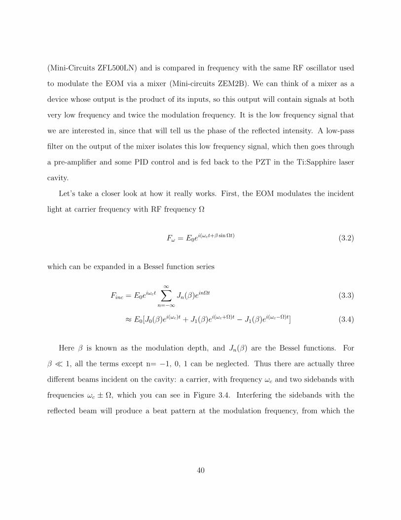
Let’s take a closer look at how it really works. First, the EOM modulates the incident
light at carrier frequency with RF frequency &
F& = E0ei(&ct+' sinΩt) (3.2)
which can be expanded in a Bessel function series
Finc = E0ei&ct
∞"
n=−∞Jn(*)e
inΩt (3.3)
, E0[J0(*)ei(&c)t + J1(*)e
i(&c+Ω)t % J1(*)ei(&c−Ω)t] (3.4)
Here * is known as the modulation depth, and Jn(*) are the Bessel functions. For
* - 1, all the terms except n= %1, 0, 1 can be neglected. Thus there are actually three
di"erent beams incident on the cavity: a carrier, with frequency 'c and two sidebands with
frequencies 'c ± &, which you can see in Figure 3.4. Interfering the sidebands with the
reflected beam will produce a beat pattern at the modulation frequency, from which the
40
phase can be determined.
Fref = E0[F ('c)J0(*)ei&ct + F ('c + &)J1(*)e
i(&c+Ω)t % F ('c % &)J−1(*)ei(&c−Ω)t] (3.5)
where F ('c) is the reflection coe!cient for a Fabry-Perot cavity with lossy mirrors at
frequency 'c. Instead of the amplitude, the intensity is measured by a photodiode, which is
given by Pref = |Eref |2, and after some algebra [56]
PcPsRe[F ('c)F∗('c + &)% F ∗('c)F ('c % &)] cos(&t)
+ Im[F ('c)F∗('c + &)% F ∗('c)F ('c % &)] sin(&t)
+ (2& terms) (3.6)
The & term in (3.6) comes from the interference between the carrier and the sidebands
and thus contains the phase information. Depending on the modulation frequency &, either
the sine or the cosine term always vanishes [56], and the remaining one is used for the error
signal. Then the phase term is extracted by a mixer, a phase shifter and a low-pass filter.
The mixer multiplies its two inputs and only when the two inputs have the same frequency
components, it produces some DC (very low frequency) signal. In our case, the DC signal
only comes from the & term in (3.6) and this can be easily isolated from the other high
frequency terms with a low-pass filter. The phase shifter is necessary to compensate for
possible phase delay due to di"erent signal paths.
The error signal as shown in Figure 3.4 is fed to a low-noise amplifier, and the gain
and the cut-o" frequency are optimized. After choosing the correct parity and DC o"set,
the signal is separately fed to a two-stage integrator (f3dB = 2 Hz and f3dB = 0.5 Hz)
41
Figure 3.4: Pound-Drever-Hall error signal (top) and transmission signal (bottom) [25]
and a proportional loop whose outputs are subsequently recombined in a summing junction.
Passing through a high voltage amplifier, the PDH error signal is applied to PZT1 (in Figure
3.1 and 3.5) inside the Ti:Sapphire laser cavity.
The detailed procedures for locking the Ti:Sapphire to the PDH cavity are the following:
First, stop scanning the Fabry-Perot cavity by switching o" the function generater (FG) in
the summing box '2 (Figure 3.5). Second, adjust the DC o"set in summing box '2 so that
the transmission of PD2 rises up close to the original height of the transmission peaks on
the scope indicating that the cavity is close to resonance. Third, switch on S1 and S2, then
adjust simultaneously the gain of the two integration stages to smooth the locking signal
and minimize the deviation of the locking signal from the resonance peak (zero on the error
signal). Sometimes, if the transmission signal jumps up and down, it might indicate mode
42
for!experiment
PBS
He*!cell
photodiodes
GP
GP
Figure 3.5: Stabilization electronics for the blue laser system [25][44]
43
hopping in the Ti:Sapphire laser, which can be confirmed by looking at the transmission
signal of the reference Fabry-Perot cavity. To get rid of the extra mode, we might need to
turn o" the PDH lock, and adjust the etalon and the DC o"set on the Ti:Sapphire PZT.
3.2.3 Saturation Absorption Spectroscopy
The PDH setup serves to stabilize the Ti:Sapphire laser on a short time scale, but can’t
compensate for slow frequency drifts due to ambient temperature changes. To keep the blue
light on resonance, we need a standard frequency reference which is immune to environmental
drift. Since we want to drive the 23S1 " 33P2 transition using blue light, this transition itself
is a good reference. Therefore, we use Saturation Absorption Spectroscopy (SAS), which is
a commonly used technique for this purpose [53][54], to lock the PDH cavity while using the
PDH cavity to lock the Ti:Sapphire laser.
When a weak laser beam passes through a cell filled with a gas of low density, it will
be partially absorbed and scattered if the laser frequency is on resonance with a electronic
transition. So if we scan the frequency of the laser across the transition, it leads to a dip in
the transmission signal. However, because the atoms are moving with di"erent velocities, the
dip is Doppler broadened, which makes the width much bigger than the natural linewidth
(see Figure 3.6(a)).
For a highly saturated pump beam (with intensity a lot higher than the saturation in-
tensity Is = 3.31 mW/cm2), due to power broadening, the spectral width of the absorption
signal is #'sat = ((1 + s)1/2, which is determined by the natural width ( and the satura-
tion parameter s = I/Isat, where Isat ="hc3(3$ [5] is the specific saturation intensity of the
atoms (h: Planck’s constant, c: speed of light, + : atomic lifetime). If there is another weak,
counter-propagating beam with the same frequency ', which equals the atomic resonant
44
Tran
smis
sio
n S
ign
al w
ith
Pum
p B
eam
!!0
v
v v
v v
v
(1)
(1)
(2)
(2)
(3)
(3)
Tran
smis
sio
n S
ign
al w
ith
ou
tPu
mp
Bea
m
!
"!D
N2(v) N
2(v)
N1(v) N
1(v)N
1(v)
N2(v)
(a)
(b)
(c)
Figure 4.4(a) In the transmission signal without the pump beam the atomic transitionis Doppler broadened.(b) When the pump beam is present, a small Doppler free signal can be seenon top of the broad dip due to saturation e!ects.(c) Only if the laser is resonant with the atomic transition the pump beam andthe probe beam talk to the same velocity group of atoms v! ! 0. That leadsto a higher transmission of the probe beam since the stronger pump beamsaturates the absorption of that velocity group.
59
Figure 3.6: (a)The transmission signal of the probe beam is Doppler broadened when thepump beam is not present. (b)The transmission of the the probe beam in the presence ofthe pump beam. Note here is a small Doppler free signal on top of the broad dip. (c) If thelaser is o"-resonance, the probe and the pump beams are interacting with di"erent velocitygroup and the transmission signal is the same as without the pump beam as shown in (1)and (3). The dip occurs only when the laser beam is on resonance and both beams interactwith the same velocity group, v=0 as in (2).
45
frequency '0, both beams interact with the same velocity group. Then the saturation of the
transition by the strong pump beam results in a reduced absorption (enhanced transmission)
of the weak beam, which you can see as a small Doppler-free signal ( called “Lamb dip”)
on top of the broad dip as shown on Figure 3.6 (b). After subtracting the transmission
signal with and without the strong pump beam, only the Doppler-free Lamb dip remains,
whose width is on the order of the natural linewidth. If the two beams are o"-resonance
(' .= '0), the probe and the pump beams are interacting with di"erent velocity groups and
the transmission signal is the same as without the pump beam as shown in Figure 3.6 (1)
and (3).
In our setup for the experiment, we have a Helium cell with a discharge driven by an
HP3200B oscillator at 57 MHz whose output is amplified by a RF Power Labs Inc model
FK 250-10C wideband RF Amplifier to 10W. This RF power is high enough to create He
metastables. A small part of the blue light from the frequency doubling cavity is split o" by
a polarization beam splitter (PBS) for the SAS. And the beam is split again into two weak
beams (probe and reference) and one strong counter-propagating beam (pump). The pump
beam overlaps with the probe beam, so that the probe beam is weakly absorbed. Transmitted
beams of the probe and the reference are collected by two separate photodetectors (in Figure
3.1 and 3.5). Comparing the two signals out of the photodetectors ends up with a Lamb
dip on the scope while we scan the laser frequency. Our saturation parameter s (s = I/Is)
for the pump beam is about 15 (Is = 3.31 mW/cm2) while for the probe beam and the
references it is about 1. The balance of the two photodetector signals is done by adding a
variable filter (F) to change the relative intensities of the probe and the reference beam.
The remainder signal after subtraction of the two photodetector signals is sent to a lock-
in amplifier (SRS Model 510) and modulated by a 800 Hz reference signal from a function
generator (Model 124A EG&G). The mechanism of generating an error signal is the same as
46
Figure 3.7: SAS signals for: (a) 23S1 " 33P2 transition and crossover between 33P2 and 33P1
(b) 23S1 " 33P2 transition (bottom) and resulting error signal (top) [25]
47
in the PDH locking technique, as explained in the previous section. Through the summing
box when the switch S4 is closed, the reference signal also modulates the PDH cavity, thereby
modulates the Ti:Sapphire laser as well as the blue light out from the frequency doubling
cavity when the Ti:Sapphire laser is locked to the PDH cavity. The SAS absorption and the
error signal are shown in Figure 3.7, in which the horizontal axis is converted to frequency
with the separation between the real peak and the crossover peak.
In the case of multiple atomic levels, so-called cross-over peaks are observed. These lie
exactly halfway between two accessible transitions that have a frequency separation less than
the Doppler broadened linewidth #'D . Figure 3.7 shows the 23S1 " 33P2 transition and
crossover between 33P2 and 33P1. This is caused by the velocity distribution bringing one
level to resonance in the probe beam and a di"erent level to resonance in the pump beam
at the same time .
To really lock the blue light on atomic resonance, we first need to find the correct SAS
absorption peak. In order to do this, we first make sure the wavemeter (Burleigh WA 1500)
reads about 777.951 ! 777.952 nm and close the Switch S3 to scan the Ti:Sapphire cavity
with the function generator at 20 Hz (Figure 3.5). Then with blue light locking on, adjust
the DC o"set in the summing box '1 until the absorption peak appears as shown in Figure
3.7. Keep tuning the DC o"set towards higher wavelength to make sure there are no more
peaks at higher wavelength, because the energy level of 32P2 is the lowest among all di"erent
J levels. After we find the right peak, we turn o" S3 and lock the Ti:Sapphire to the PDH
cavity (see Section 3.2.2). The next step is to lock the PDH cavity to the atomic transition.
The switch S6 is set to scan and we turn on the switch S5 (Figure 3.5), then we change the
DC o"set of the summing box '2 until we can see the absorption signal as shown in Figure
3.7(b) again. The size of the absorption signal depends on the gain G5. If G5 is increased,
the crossover peak, which is exactly half way between two real transitions (23S1 " 32P2 and
48
23S1 " 32P1), can be seen together with a real peak as shown in Figure 3.7(a), separated
by 330 MHz. Afterwards, switch on S4 and turn up G4 a little bit so that we can see the
error signal. If G4 and G5 are turned up too much, the PDH transmission and error signal
will become very noisy. After everything is set correctly, finally switch S6 from scan to lock,
then the laser should be locked.
3.3 Red Light System
The red laser system is much simpler than the blue laser system. It is also based on a
Ti:Sapphire laser, the Tekhnoscan Model TIS-SF-07e. In the past, it was pumped by an
Argon-Ion laser (Coherent Innova 310) and the output power was around 1 W at a pump
power of 10W [25]. But after several years, the best the Argon-Ion laser could produce was
around 7 W, and we could only get 500 ! 600 mW out. In Oct. 2008, we replaced the Argon-
Ion laser with a new Verdi V10 laser, the same model as the one used for pumping the SEO
Ti:Sapphire. After careful alignment, we reached an output power of 1.3 W, horizontally
polarized and with linewidth < 3 MHz, with 9 W 532 nm pump light. Compared with the
SEO Ti:Sapphire which is pumped by the same amount of 532 nm light, the Tekhnoscan
has a relatively lower pumping e!ciency. This is probably caused by several factors: first,
the quality of the Ti: Sapphire crystal is not as good as the one in the SEO laser. Second,
as shown in Figure 3.8 [25], the ring geometry is di"erent, as the Tekhnoscan contains more
mirrors and more mode-selective components and lastly, the coatings on the components
may be inferior.
The laser cavity is comprised of six mirrors, two of which are spherical (M1 and M2)
used to focus the light onto the Ti:Sapphire crystal and the others are planar. A Faraday
rotator together with an out-of-plane mirror (M5) ensures a unidirectional running wave in
49
M"#
M"$
M$ M%
M#
M& M'
M(
!" $%&'(')'r + r','r'-.' .%&/)0
Figure 3.8: Optical scheme of the red laser system
50
the cavity. For the first alignment from scratch, it is much easier to start in the standing
wave mode, with mirror M4 and M6 reflecting beams back along their original path. Then we
can even take out more elements from the cavity: the birefringent filter, the thin etalon, the
Faraday rotator and the thick etalon assembly. Try to get it to lasing and use a fast power
meter to peak the laser alignment for maximum power. Next, put the birefringent filter,
thick etalon and Faraday rotator back, one at a time in this order. Since the birefringent
filter and the thick etalon shift the beam horizontally a lot, the beam passing through them
might not hit M6 anymore. It is better to put a bigger auxiliary mirror there first, otherwise,
we will just have to move the M6 mirror base and redo part of the alignment. After we got a
decent amount of light, say higher than 600 mW, in the standing wave mode, we can switch
back to the ring configuration by using horizontal and vertical controls of M4 and M6 to
reflect the fluorescent spot onto M5, and to reach coincidence. Finally, we can put the thin
etalon back in the beam, which should not cause much loss. Always adjust in turn mirrors
M4, M6 and Mp2 for maximum power.
One advantage of this Ti:Sapphire laser is that it comes with an electronic control unit.
The control unit is able to allow adjustment of the mode selective elements inside the cavity
to tune or scan the frequency and also automatically maintain the single frequency generation
mode [57].
We can tune the wavelength over a very wide range: 770 ! 837 nm, which makes it
possible for us to excite helium atoms to all di"erent n states (from n = 12 to 30 and higher).
This is done with a birefringent (BF) filter, a thin etalon and a thick etalon. The wavelength
is coarsely selected with a 3-stage BF filter which consists of three parallel crystalline quartz
plates placed at Brewster’s angle. Within a given spectral range, the filter provides minimal
loss for the radiation since it doesn’t change the polarization of the light upon passing through
each of the filter plates. For other wavelengths, the losses su"ered at each Brewster-angle
51
surface within the cavity due to the polarization change make these wavelengths fail to reach
the lasing threshold. The wavelength of minimum loss can be shifted by modifying the tilt
angle of the birefringent filter via a micrometer screw. The thin etalon is made of a 0.5
mm thick uncoated fused silica plate, which allows tuning wavelength radiation within a 207
GHz range that corresponds to the thin etalon free spectral range. A electro-mechanical
drive is used for the thin etalon tuning, which can be accessed by the “etalon” knob on the
control unit. And an air spaced thick etalon made with two Littrow prisms with thickness
of 8 mm has a free spectral range of 18.75 GHz. The spectral position of the thick etalon
transmission peak is adjusted with the help of a piezoelectric transducer (PZT). So rotate
the “Selector” knob to change the PZT voltage for the setting of wavelength with the 18.75
GHz thick etalon. Furthermore, the optical length of the cavity can be dynamically adjusted
by moving three mirrors, mounted on large PZTs, which are controlled by the “resonator”
knob on the control unit. This allows smooth tuning of the radiation wavelength within
the 5 GHz range. By adding a ramp signal on the PZTs, we can scan the laser frequency
smoothly in a range of ! 5 GHz. The wavelength of the light is monitored by the Burleigh
WA-1500 wavemeter. In addition, a small amount of light is split o" the main beam and sent
to a scanning Fabry-Perot interferometer to make sure the laser runs in the single frequency
regime.
Automatic adjustment of the single frequency mode of the laser is done by locking of
the thick etalon transmission peak. The way the frequency lock-in system works is pretty
similar to the PDH locking: the thick etalon PZT receives a small AC voltage at 1 kHz.
This modulation leads to a slight modulation in the output power at the same frequency
that is monitored by a photo-detector. (A beam split from the main beam is directed to the
photo-detector.) Further on, the photo-detector signal passes through a 1 kHz filter, then
gets synchronously detected and fed from an integrator into a high-voltage amplifier, which
52
drives the PZT of the thick etalon [57].
The out-of-plane mirror (M5) is attached to a fast PZT, which could be used for external
control. So we also set up our PDH locking system to keep it more stable, although the
frequency stability of the red light is not as critical as the blue light because we scan the
Stark energy level through resonances during the experiment. While most of the beam goes
to the experiment, a small amount is sent to a scanning Fabry-Perot interferometer to make
sure the laser runs in the single-frequency regime.
3.4 1083 nm Light
The light at ! = 1083.33 nm used for the 23S1 " 23P2 transition is provided by a Spectra
Diode Labs (SDL) model SDL-6702-H1 distributed Bragg reflector (DBR) diode laser. This
diode is packaged in an 8 pin TO-3 window mount with a thermistor and a thermoelectric
cooler. The temperature of the diode is kept stable at 21.9 ± 0.1oC by an ILX Lightwave
LDT-590 temperature controller and the current of the laser diode is set with a Thorlabs
LDC 500 laser diode controller. The dependence of the laser diode wavelength and output
power on its current has been examined very carefully in previous theses [58][47][55].
The linewidth of the diode is about 3 MHz, which is larger than the 1.6 MHz natural
linewidth of the 23S1 " 23P2 transition. To narrow the linewidth of the diode laser, an
extended cavity is used, as seen in Figure 3.9. 30% of the diode output is picked o" by
a plane beamsplitter and sent to a retro-reflecting mirror, which is mounted on a piezo-
electric transducer (PZT). This controlled feedback increases the lifetime of the photons in
the cavity and narrows the linewidth to approximately 125 kHz [59]. For shielding against
external temperature fluctuation and vibration, the diode and the extended cavity set-up
are placed on a 305 mm x 710 mm x 76 mm Aluminum slab and inside a box constructed
53
Figure 3.9: Schematic of the diode laser setup [55]
of polystyrene foam insulation. Although there are long-term temperature drifts over the
course of a day, the temperature inside the box is stable to better than 0.5 oC/hr in a short
term [55]. In addition to narrowing the bandwidth, the extended cavity also serves as the
diode’s fine frequency tuning knob.
As a result of the external cavity setup, the diode produces two beams: a main beam (70%
of full power) and a leakage beam (21% of the full power). To prevent disruptive feedback
to the extended cavity, optical isolators are placed in both beams. After collimation, these
beams are launched into single mode optical fibers. The main beam is used for the four
frequency setup to feed the Fiber amplifiers and the leakage beam is used for Saturated
Absorption Spectroscopy (SAS) to lock the laser frequency to an atomic transition in He.
54
Figure 3.10: Schematic of the SAS setup for the 1083 nm light [55]
3.4.1 Frequency Locking
SAS locking has been described in detail in the blue light section. Figure 3.10 and 3.11
show how it is implemented. A thick glass plate reflecting 4% from each surface is used to
produce the probe beam and the reference beam. These two beams are directed through a
Helium discharge cell and transmitted through a 50/50 beam splitter and detected on the two
photodiodes. The transmitted beam through the thick glass plate is directed to a mirror and
then the 50/50 splitter. Its reflection o" the beam splitter is directed to counter-propagate
against the probe beam. The reference signal is subtracted from the probe signal to obtain
a Doppler-free spectrum.
The SAS absorption signal is first amplified with a Stanford Research System (SRS)
SR560 low-noise preamplifier and then fed into an EG&G Princeton Applied Research lock-
55
DBR Laser Diode
Modulation10 kHz
Laser DiodeCurrent
Controller
Laser DiodeTemperature
Controller
Lock-InAmpli!er
SAS Signal
AnalogPID Controller
Low-NoisePreampli!er
Error Signal
Extended Cavity PZT
Figure 4.6 Schematics of the locking electronics. Details about the componentscan be found in the text.
4.2.3 O!-Resonance Locking
For locking the laser to atomic resonance, i.e. ! = !a, the secondary output
of the extended cavity of the laser (see figure 4.3) is used for the SAS (see
figure 4.7 for the SAS signal and the error signal). In this case the +kv
beam contains a component of !a and a push of atoms can be detected on the
MCP/Phosphor Screen. Therefore that locking scheme is used for aligning the
+kv beams to which all other beams are aligned afterwards.
For bichromatic collimation on the other hand it is necessary to lock the
62
Figure 3.11: Schematic of the SAS locking electronics for the 1083 nm light [47][55]
in amplifier (model 5104). To generate an error signal, a modulation signal must be applied
to the laser frequency. This modulation signal also serves as the reference signal for the lock-
in amplifier. The 10 kHz reference signal is provided by an SRS DS345 30 MHz synthesized
function generator. It modulates the current driving the laser diode and therefore modulates
the laser frequency. The error signal is sent to an SRS SIM960 analog proportional-integral-
derivative PID controller, whose output goes to a high voltage amplifier and then feeds back
to the PZT in the extended cavity to force the laser frequency to remain on the atomic
transition.
3.4.2 Bichromatic Light
As the name suggests, bichromatic light consists of light at two frequencies, '0 ± $.
This is produced by double passing the light from the diode laser through an acousto-optic
56
modulator (AOM) driven at a frequency $/2" [60], as shown in Figure 3.12. The resulting
two beams have the spectral components ('0, '0 + 2$) and ('0 + $, '0 % $) respectively.
Both beams are used for bichromatic collimation in the lithography experiment [47][55], but
to push the metastable He atoms out of the beam here, we only use the ('0 + $, '0 % $)
beam. Since the bichromatic light setup is in an adjacent laboratory, we pick o" the beam
we need with a flip mirror and send to our room with a polarization maintaining (PM) fiber.
A power of 1 mW exits from the fiber. To make sure that the two frequencies have the same
intensity, a mating sleeve and an extra single mode fiber are used to transport the beam to
a Fabry-Perot cavity. Monitoring the Fabry-Perot transmission signal allows the intensities
of the two frequencies to be balanced by adjusting the Bragg angle of the AOM.
The AOM is driven at 60 MHz ($/2" = 60 MHz) by an HP 3200B which is amplified by
a MiniCircuits ZHL-1-2W RF amplifier. For the bichromatic force to work at this detuning,
the beam needs an intensity of ! 4000s0 (s0 is the saturation intensity for the 23S1 " 23P2
transition, 0.17 mW/cm2) [58][47]. This is accomplished by sending the modulated light
to a Keopsys Ytterbium (Yb) - doped fiber amplifier (model KPS-CUS-BT-YFA-36-SLM-
PM-LIP-121-FA-FA) to get amplified. The pump light from internal diode lasers is injected
through a V-groove of the Yb-doped fiber to invert the population inside the fiber and thus
lead to amplification. The Keopsys fiber amplifier has three amplification stages which are
separated by optical isolators to prevent light back-reflection. It begins with a pre-amp stage,
which is supposed to saturate the input for the next two amplification stages. The next two
stages are pumped by diode lasers and we can turn up the diode’s current to get output
power of the fiber amplifier up to 5 W. In addition, this amplifier o"ers two di"erent modes:
Automatic Current Control (ACC) and Automatic Power Control (APC). In ACC mode, the
amplifier is running in order to maintain a constant set current through the pump diodes. A
variation of the input power might induce a variation of the output power. In APC mode,
57
!!"" !#"
!" !!$"
!
!!" !
Figure 3.12: Double passing an AOM produces two beam with two frequencies [55]. The('0 + $, '0 % $) beam is used for our bichromatic force.
the amplifier is regulated at a fixed output power set point. The device is running in order to
maintain a constant optical output power monitored with a photodiode. The current of the
pump diode is adjusted to drive a constant output power independent of the input power.
In order for the amplifier to operate safely, it needs to be seeded with at least -3 dBm (0.5
mW) of light. To set the polarization of the light into the input PM fiber of the amplifier, we
add a thin fiber paddle (Thorlab FPC560) for polarization control and two mating sleeves
for fiber-to-fiber connection. Although we have about 1mW out from the PM fiber between
two laboratories, after all those extra components, we only have about -2.5 dBm light into
58
the fiber amplifier, which is too close to the safety limit. Due to temperature fluctuations,
sometimes, it might be even lower than -3 dBm. So before the paddle, we first amplify the
light intensity using a OIYb30 fiber amplifier from Optocom Innovation (with maximum
output power about 1 W) to maintain the input light of the 5 W amplifier above 0 dBm.
The output from the fiber amplifier is collimated and sent transversely across our atomic
beam immediately downstream from the STIRAP beams. It is retro-reflected by a mirror,
which is set on a stage to obtain a phase delay of "/2 (Section 5.2.1). This makes the
remaining metastable atoms which are not excited by STIRAP well separated from the main
atomic beam, so that we can tell the e!ciency of our STIRAP by measuring the pushed-out
atomic flux.
59
Chapter 4
STIRAP
4.1 Introduction
For a two level atomic system, incoherent radiation could change the ratio of the atomic
populations by absorption, stimulated emission and spontaneous emission. The rate could
be calculated from the Einstein coe!cients [61]. For intense radiation near atomic resonance,
the excited state population saturates at 50%, as shown in Figure 4.1.
The case of coherent excitation is markedly di"erent. For laser light with frequency
on resonance with the atomic transition, we will see an oscillation between 0 and 1 of the
population in the excited state. The oscillation frequency is called the Rabi frequency [62][5],
which is defined by
& = % e
!E0'e|r|g( = %µE0! (4.1)
where E0 is the amplitude of the coherent field, |g( is the ground state and |e( is the excited
state, µ = e'e|r|g( is called the dipole transition moment which depends on the quantum
numbers of the states involved. And if the laser is not on the atomic resonance frequency,
60
Figure 4.1: Evolution of the population of the upper level in a two-level system, driven bycoherent radiation, by an incoherent radiation field, and by an adiabatic passage process [17]
but with a detuning $, the e"ective Rabi frequency is
&eff =/&2 + $2 (4.2)
The oscillation period gets shorter and the maximum population of the ensemble in the
excited states goes down from 1 to (&/&eff )2, as shown in Figure 4.2. A light pulse with
$ = 0 and interval of T which satisfies &T = ", transfers the atom from the ground/excited
state to the excited/ground and is called a "-pulse.
A robust method for achieving e!cient population transfer is adiabatic rapid passage
(ARP). The frequency of the external field is slowly tuned across the atomic resonance from
below resonance to above resonance or in reverse. The time scale of this frequency sweep
must be slower than the Rabi frequency, but faster than the spontaneous emission rate.
In the Bloch sphere picture, the Bloch vector precesses around &eff at the frequency $.
61
Figure 4.2: Rabi oscillations with and without detuning. When the laser is detuned awayfrom resonance full population inversion no longer occurs and the oscillation period getsshorter.
Consider atoms in the ground state (south pole of the Bloch sphere) and a laser detuned to
the far red side of resonance. By sweeping the detuning $ through zero, the Bloch vector
will follow &eff and end up parallel to |&eff | in the excited state (north pole of the Bloch
sphere). A more detailed description about ARP can be found in previous Ph.D. theses
[63][64].
In our case, to excite the atoms from the metastable state to high Rydberg states, we need
to do a two-photon transition in a three level system. In an intuitive excitation order, due to
spontaneous emission and stimulated emission from the intermediate state, we could not get
an average e!ciency higher than 25%. So we use the technique called “Stimulated Raman
Adiabatic Passage” (STIRAP), which permits the complete transfer of population between
two quantum states. In essence, this procedure uses a pump pulse (near resonant with
transition 1-2) and a Stokes pulse (near resonant with transition 2-3) to achieve complete
62
transfer of population between states 1 and 3. For this to occur, it is important that the
Stokes pulse interact first (counterintuitive pulse order), that the pulses satisfy a few simple
constraints on peak value and smoothness, and that the pulse frequencies together satisfy a
two-photon resonance condition.
Hioe and Eberly’s 1981 paper [65] first described this process in terms of an N-level
coherence vector and its rotations. They continued their work with a paper concentrating
on a three level system, which Hioe later developed as “generalized adiabatic following” or
STIRAP. In this subsequent paper [66], the situation of a three-level system was addressed,
including the use of pulsed light to drive the transitions. Interestingly, even though the
use of pulses separated by a delay is mentioned, these papers do not specifically address
the situation of the pulses arriving in the counter-intuitive order, i.e., the pulse driving the
upper transition coming before the pulse driving the lower one, which is the hallmark of the
STIRAP process. Among the first experiments to use the counter-intuitive pulse order was
the switching of population between molecular vibrational levels by Klaas Bergmann and his
colleagues in 1988 [67]. It was in 1990 in a subsequent paper [68] by the same group that the
acronym STIRAP was coined. STIRAP experiments may be performed on an atomic (or
molecular) beam, with “pulses” generated by the atoms passing through spatially separated
laser beams perpendicular to the path of atoms. Alternatively, a sample of atoms can be
illuminated by pulsed lasers with a time delay.
4.2 STIRAP Theory
Stimulated Raman Adiabatic Passage (STIRAP) combines features of the process of
stimulated Raman scattering and adiabatic passage. A simple analysis of the STIRAP
process for a three level system is given [69]. The three levels have eigenvector |1(, |2( and
63
Figure 4.3: Three level # (a) and ladder (b) excitation scheme. #P (#S) are the detuningsfor pump (Stokes) light and &P (t) (&S(t)) are the Rabi frequencies of the pump (Stokes)light
|3( with a pumping light connecting the first two levels |1(, |2( and a Stokes laser connecting
levels |2( and |3(. Under the rotating wave approximation (RWA), the Hamiltonian for the
three level system, including the atom-field interaction, is:
H =!2
$
%%%%&
0 &P (t) 0
&P (t) 2#P &S(t)
0 &S(t) 2(#P ±#S)
'
(((()(4.3)
where the &P (t) and &S(t) are the Rabi frequencies of the pumping light and the Stokes
light respectively, and #P and #s are the detunings of the pumping field and the Stokes
field, as shown in Figure 4.3. #P = (E2 % E1)% !'P , #S = (E3 % E2)% !'S. ('P and 'S
are the frequencies of pump and Stokes fields.)
In the 3-3 position of the Hamiltonian matrix, the plus sign is taken when the three-level
system is a ladder (or cascade) configuration, and the minus sign is used in Lambda or Vee
64
configurations. In the case of STIRAP, the two-photon resonance condition between states
|1( and |3( should be fulfilled, so this 3-3 term should be zero, i.e., %P = ±%S = %. The
eigenvalues !'k of the Hamiltonian in Eqn. 4.3 yield the instantaneous energy corresponding
to the instantaneous eigenstates |ak(t)(:
'+(t) = #+#&2
P + &2S +#2
'0(t) = 0
'−(t) = #%#&2
P + &2S +#2
(4.4)
with eigenstates given as a superposition of the bare states |1(, |2( and |3(
|a+(t)( = sin) sin,|1(+ cos,|2(+ cos) sin,|3(
|a0(t)( = cos)|1( % sin)|3(
|a−(t)( = sin) cos,|1( % sin,|2(+ cos) cos,|3(
(4.5)
Here )(t) and ,(t) are defined as
tan)(t) = %&P (t)
&S(t)(4.6)
tan 2,(t) = %#&P (t)2 + &S(t)2
# (4.7)
The eigenstate |a0(t)(, known as the trapped state, is of particular interest since this
eigenstate does not involve the bare intermediate state |2( at all. In the case that the lifetime
of the intermediate state is shorter than the interaction time, populating the intermediate
state would be really deleterious due to its spontaneous decay, and would lead to a significant
unwanted loss in transferring population to the final states. As for our experiment, the
lifetime of the intermediate 33P2 level is about 107 ns. Hence, if we can make sure that the
65
real time state vector |$(t)( is tied to the trapped state |a0(t)( during the whole interaction
time, then the intermediate state will never be populated.
Then if we let ) start at zero and go to "/2, this trapped state eigenvector evolves from
|1( to |3(, providing e!cient population transfer from initial state to the final state. To
achieve this, we need to control the Rabi frequencies of the pump and Stokes laser in a
suitable way, satisfying the following condition [70]:
&P (t " %0)
&S(t " %0)" 0,
&S(t " +0)
&P (t " +0)" 0 (4.8)
This corresponds to a counter-intuitive pulse ordering, as shown in Figure 4.4. We can
identify three distinctly di"erent time intervals 1, 2 and 3. In interval 1, only the Stokes laser
is present, and the mixing angle ) is zero. Therefore, the state |a0( is identical to |1( as well
as the state vector |$( since the atom starts in this state, i.e. the three vectors are aligned
(see Figure 4.5). In the interval 2, the Stokes laser Rabi frequency is smoothly reduced while
the pump laser Rabi frequency increases to its maximum value, changing the mixing angle
smoothly form 0 to "/2. As shown in Figure 4.5, the vector |a0( is rotated into a position
parallel to the bare state |3( in a plane perpendicular to the bare state |2( because |a0( has
no |2( component.
In the region where the Stokes light is very strong and pump beam is very weak, the
energy level of the two higher levels are shifted too far o" resonance so that the pump light
does not produce excitation from the level |1( to intermediate level |2(. Since the same
mechanism leads to electromagnetically induced transparency (EIT), this region is called
“pump induced EIT phase”. Similarly, in the region where the pump light is very strong
and the Stokes light is very weak, the weak Stokes light is not going to result in any stimulated
emission from |3( to |2(. It is called “Stokes induced EIT phase”.
66
Figure 4.4: Time evolution of (a) Rabi frequencies of the pump and Stokes beams, &P , &S;(b) the mixing angle ), (c) the dressed state eigenvalues '0,±; and (d) the population of theinitial level |1( and final level |3( [17].
67
!
Figure 4.5: State vector |$( for the three level system in the basis of the bare states (|1(, |2(and |3() and in the basis of the dressed states (|a0(, |a+( and |a−() [17][70].
We can also look at the evolution from the aspect of the eigenvalues, as shown in Figure
4.4 (c). At very early times, both Rabi frequencies are zero, all three dressed state eigenvalues
are degenerate as ' = 0. Later in region 1, the degeneracy of the eigenvalues is lifted due to
the coupling between states |2( and |3( from the Stokes laser. The eigenvalue that remains
unchanged is associated with |a0(. In interval 2, the splitting of the eigenvalues is the largest
since the coupling is strongest and both pump laser and Stokes laser contribute to it as
in Eqn. 4.4. In the meantime, if the state vector |$( evolves adiabatically, it follows |a0(
and moves from its position parallel to state |1( to a position parallel to state |3( as shown
in Figure 4.5, which results in complete population transfer. If the coupling is insu!cient
(nonadiabatic), the motion of the state vector will lag behind the motion of the dressed
68
states and it will precess around |a0(, then the state vector acquires a component along |a+(
or |a−(. This means that some population will get to the leaky intermediate state and the
transfer process is incomplete.
4.3 Conditions for STIRAP
4.3.1 Adiabatic Following
For the greatest e!ciency in adiabatic passage, non-adiabatic coupling must be small.
The Hamiltonian matrix element for nonadiabatic coupling between the trapped state |a0(
and the states |a±( is given by 'a±|a0( [17]. Nonadiabatic coupling is small if this matrix
element is small compared to the field induced splitting |'± % '0| of the energies of these
states, i.e.,
|'a±|a0(| - |'± % '0| (4.9)
Using equations (4.5) to express the strength of the nonadiabatic coupling, we have
|'a+|a0(| = %) sin,
|'a−|a0(| = %) cos,(4.10)
and therefore the adiabatic constraint simplifies to [68]
|)| - |'± % '0| = #±*
&2P + &2
S +#2 = &eff (4.11)
In the case of one photon resonance (# = 0), &eff =#&2
P + &2s. From the definition of ),
Eqn. (4.6), we have
|)| = |&P&S % &S&P
&2P + &2
S
| - &eff (4.12)
69
Adiabatic following is satisfied as long as Eqn. (4.12) holds throughout the whole in-
teraction time. This can be evaluated for any time t with given laser pulses, so it is called
the “local” adiabaticity criterion. When the laser pulses have a smooth shape, a “global”
adiabaticity criterion may be derived from Eqn. (4.11) by taking a time average of the left
side. If the pump and the Stokes pulse overlap in a time interval %+ , the total angle change
is "/2, ')( = "2∆$ , so the global criterion essentially is
&eff%+ 1 1 (4.13)
It is recommended to keep &eff%+ larger than 10 based on experimental results and nu-
merical simulations. There is a limit, too, to how small the Rabi frequencies can be. Usually,
they have to be much larger than the natural linewidth of the corresponding transition.
4.3.2 Detunings from One-Photon and Two-Photon Resonance
In contrast to the case of perfect adiabatic evolution, beyond the adiabatic limit, the
intermediate-level detuning does a"ect the transfer e!ciency. This is so because the in-
termediate detuning is involved in the adiabaticity condition and for any fixed pulse area
defined as+ +∞−∞ &s,p(t)dt, the adiabaticity deteriorates as % increases. The transfer e!ciency
vanishes at very large detuning. If we define $1/2 as the intermediate detuning at which the
final state population equals 1/2 (essentially the half linewidth), it has been demonstrated
that $1/2 grows with the square of the pulse area [71]. $1/2 , c&2, where & is the pulse area
and the coe!cient c may depend on the pulse shapes, the pulse delay, etc., but not on &.
In the case of detuning from two-photon resonance, the linewidth increases only approx-
imately linearly with the pulse area [72]. It was shown that for a characteristic time of the
pulses greater than the spontaneous decay time of the intermediate state, the two-photon
70
Figure 4.6: Numerically calculated transfer e!ciency in STIRAP vs. the sum and thedi"erence of the pump and Stokes detuning (i.e. e!ciency vs. the single photon and two-photon detunings) for Gaussian pulse shapes, &P = &0exp[%(t% +)2/T 2], &S = &0exp[%(t++)2/T 2], with &0T = 20, + = 0.5T [73].
lineshape for population transfer using STIRAP is close to Gaussian. Based on these facts,
STIRAP is much less sensitive to single photon detuning than to two-photon detuning [73],
as shown on figure (4.6). Figure 4.6 is for a # system, so the horizontal axis shows the
two-photon detuning and the vertical axis shows single photon detuning.
If the intermediate state is far detuned so that the detuning is a lot larger than the Rabi
frequencies &P (|1( % |2() and &S (|2( % |3(), then the three level system reduces to a two
level system [74]. Thus, the two-photon Rabi oscillation between the first level and the third
level with respect to two-photon interaction time would be seen, as in [75]. This is di"erent
71
from our adiabatic condition.
Generally speaking, if the pulses are coincident or are in the intuitive order, Rabi oscil-
lations result and the system is sensitive to laser parameters, In the counterintuitive order
and with Eqn. (4.13) satisfied, the system is relatively insensitive to these parameters.
4.3.3 Pulse Delay
The objective of the delayed-pulse scheme is to maximize the projection of the vector
representing the bare state |1( onto the state |a0(, i.e. |'1|a0(|. For overlapping beams, state
|1( has nonvanishing components along all states |a0(, |a+( and |a−(, and only the projection
on |a0( can be used for e!cient population transfer, because the population of the other
states may be lost through radiative decay. For large delay, |'1|a0(| approaches unity at
earlier times. However, if the delay is too large, then the adiabatic condition (Eqn. 4.11)
may be poorly satisfied and nonadiabatic transitions would lead to population loss. It has
been calculated that for the optimum delay, the mixing angle should reach an angle of "/4
when &eff reaches its maximum value [17].
To prove that the STIRAP mechanism works with a counter-intuitive pulse order, we
measured the relative transfer e!ciency as the overlap between the laser beams is varied
with all other parameters, such as laser frequencies and intensities, remaining unchanged.
Figure 4.7 shows a typical result of our measurements.
The data is taken from an ion detector, which is downstream from our interaction region
and monitoring the Rydberg atoms that are ionized after STIRAP, as shown in Figure 2.4
and 2.5. The horizontal axis shows the scanning of the DC electric field in one period (10
Hz). In the first half of the scan the field increases, and in the second half it decreases, so
essentially the two sets of peaks are identical. The peaks indicate that excitation to Rydberg
72
levels occurs as we scan through our Stark map. Both of the laser beams are collimated by
cylindrical telescopes to an elliptical shape. The intensity FWHM of both the red and blue
beams is about 500 microns horizontally (along the atomic beam direction) and 2.0 mm
vertically. The reason that we make both beams much larger than the atomic beam size
is that we want to make sure that the atoms at the beam edge see close to the same light
intensities to maintain equal Rabi frequencies to the atoms in the beam center. We set the
two beams in a co-propagating configuration by using a dichroic mirror which reflects blue
light and transmits red light. The dichroic mirror is on a precision stage, and by moving
the position of this stage, we can easily change the blue light position with respect to the
red. The blue beam position axis tells us the relative position of our red and blue beam. In
the positive region, the blue light is ahead of red, in the intuitive order and in the negative
region, the red light is ahead of blue, in the counter-intuitive order. Zero is where the two
beams are overlapping. Here, we can clearly see that when the red beam us ahead of blue
by 0.5 mm (! 0.5 µs delay time), the peak signal is about 3 times larger than the signal
when red and blue are overlapping. The peak Rabi frequency is about 25 MHz for the blue
light and 17 MHz for the red light, so the adiabatic condition &effT 1 1 is satisfied.
By comparing ion signals with di"erent relative positions of red and blue light, we have
confirmed that STIRAP is an e!cient way to improve our population transfer rate, but to
get an absolute value of the STIRAP e!ciency, we need an absolute measurement. Absolute
e!ciency measurements will be discussed in the next chapter.
73
Figure 4.7: Ion detector signal showing relative population transfer from the He metastablestate (23S1) to the 243S1 state as a function of the overlap between the Stokes (red) andthe pump (blue) lasers. The positive region is where the blue light is ahead of the red, inthe intuitive order and the negative region is where the red light is ahead of blue, in thecounter-intuitive order. At zero, the two beams are overlapping.
74
Chapter 5
Absolute Measurements of STIRAP
E!ciency
5.1 Introduction
To measure the absolute excitation e!ciency for STIRAP, we need an e"ective way to
distinguish the He* atoms that are excited to the Rydberg state from those that remain
in the metastable 23S1 state. In previous papers, the absolute e!ciency measurements of
STIRAP were mostly based on field ionization, photoionization or fluorescence [20][21]. For
example, Cubel at al. [22] used two STIRAP stages and counted the Rydberg 85Rb atoms
by field ionization after the first and the second STIRAP stage. By comparing these two
counts, they got a phenomenological e!ciency of 50%, and after corrections, they claimed a
maximum e!ciency of about 70% near the center of the excitation region.
We first measured the absolute e!ciency of STIRAP excitation using radiation pressure
from a 30 mm wide curved wavefront light beam of ! = 1083 nm to deflect residual 23S1
metastable atoms out of the atomic beam. In this way, the metastable atoms are spatially
75
separated from the rest of the beam and we counted their flux with and without the STIRAP
beams with the SSD detector after flight on a long beam path. More recently, we further
narrowed down the deflection region in order to lower the decaying probability from the
Rydberg states back to the metastable state before and during the deflection process, using
the bichromatic force, which is much stronger than the radiative force. If our STIRAP
e!ciency is 100% so that all the metastable He* atoms are excited to Rydberg states, the
1083 nm bichromatic beam is not going to cause any deflection, because there are no residual
23S1 atoms and only such atoms can be deflected. On the other hand, if there is no Rydberg
excitation at all, we will see the highest deflected flux and this can be calibrated by using the
bichromatic beam and blocking the STIRAP beams. Therefore, the ratio of the deflected
flux measured with STIRAP beams on and o" provides an absolute measure of the fraction
of the atoms remaining in the 23S1 state, from which we get the STIRAP e!ciency with
high absolute accuracy.
5.2 Experimental Setup
Figure 5.1 shows a top view of the setup for the absolute e!ciency measurements. About
23 cm downstream from the source, a 0.3 mm wide by 0.5 mm high aperture is used to
collimate the atomic beam. After 26 cm further, the red (790 ! 820 nm) and the blue
light (389 nm) are incident perpendicularly to the atomic beam in a counter-intuitive order
to do the STIRAP excitation from the metastable He* state to a highly excited Rydberg
level. Both beams are linearly polarized in the vertical direction along the electric field, and
their intensity FWHM is about 0.5 mm along the atomic beam direction and 2.0 mm along
the vertical direction. Because the vertical beam waist size is large (1.7 mm), even atoms
at the vertical extreme of the atomic beam experience a Rabi frequency that is more than
76
He* beam1070±240m/s
796nm 389nm
Deflected residual He* atoms
1083nm
Measured by SSD detector
MCPPhosphor screen
2300V
~23cm ~26cm ~140cm
~0.25cm
~ 4.5mm
4mm
Aperture: 0.5mm(h)×0.3mm (w)
Figure 5.1: Experimental setup for the absolute e!ciency measurements for STIRAP.
80% of the maximum at the center. After this interaction region, the atomic beam consists
of Rydberg atoms, residual metastable atoms, ground state He, and some UV photons are
also mixed in the beam. Just after the STIRAP region, we use the bichromatic force from
1083 nm light, which corresponds to the transition between the metastable 23S1 state and
the 23P2 state, to deflect the residual metastable atoms out of the beam while leaving other
components unperturbed. The bichromatic beam is only 4 mm wide along the atomic beam
path, and the distance between the peak of the blue light and the edge of the bichromatic
beam is 2.5 mm. Then in the detection region, we see a deflected peak about 4.5 mm
away from the original source center and the strength of this peak changes linearly with the
residual metastable counts. Thus, measuring the SSD output current in the deflected beam
region with STIRAP beams on and o" gives us the absolute e!ciency of STIRAP.
77
5.2.1 Bichromatic Force
The bichromatic force has been described in the literature and well studied in our lab
[43][76][77]. For this experiment, we require two optical frequencies to deflect the beam. But
in the case of neutral atom lithography, four frequencies are used to collimate the atomic
beam in two dimensions [58][47][55]. The four frequency production is described in detail
in Chapter 3 Section 3.4.2. Here, a brief description will be given, explaining why the
bichromatic force is much larger than the radiative force and hence more suitable in this
experiment.
The "-pulse model for describing bichromatic forces provides an intuitive notion of how
it works. Consider a laser beam consisting of two frequency components of equal strength
and symmetric detuning above and below atomic resonance. The total electric field could
where 'A is the atomic resonance frequency, k = 'a/c and #k = $/c. From equation 5.2
we see that the beam can be described as an amplitude-modulated single carrier frequency
at the atomic resonance frequency 'a having modulation period "/$. If the intensity of the
beam is chosen so that the area under the envelope of one modulation period satisfies the "
pulse condition for the atomic transition, i.e., & = "4 $ [78], then in each modulation period
the atoms undergo a level exchange between the ground state and the excited state.
Then if we retro-reflect the modulated carrier wave back by a mirror to create a standing
wave, as shown in Figure 5.2, the atoms can first absorb a photon from the left and before
the arrival of the next "-pulse from the left, a pulse from the right will drive the atom back
78
e-
e-
e-!k
!k !k
"-pulse
"-pulse train Mirror
Phase Delay
"-pulse
"/#
(a)
(b)
Figure 5.2: The two frequencies in the bichromatic laser beam create a series of "-pulsesfrom the beat frequency. Each "-pulse excites or de-excites the atom in a time of "/$ leadingto a force (!k$/") much larger than Frad,max ! !k)/2.
79
to the ground state. The momentum kicks for the absorption and the stimulated emission
are therefore in the same direction, to the right. Since this happens with a time period of
"/$, the resulting force can be written as
F =#P
#t=
2!k$"
(5.3)
which is not limited by the radiative decay rate, ), so this force can be much bigger than
the radiative force ! !k)/2 since $ could be 1 ).
However, in order to get a large force in the correct direction, we need to control the
phase delay between the counter-propagating beams. If the phase delay is chosen so that
the sequence of "-pulses from alternating directions is evenly spaced in time, the average
force is zero. A preferred direction for momentum transfer is established by providing an
asymmetric pulse timing sequence. Because of this, the average strength of the bichromatic
force is reduced by a factor of 2, F ! !k$/" [59].
The more accurate way to describe the bichromatic force is by numerical integration of
the optical Bloch equations. Now the resulting optimum Rabi frequency becomes & =*
32$
[59][47]. For our bichromatic beam, $/(2") = 60 MHz, and the "-pulse length is 250 cm. To
satisfy the "-pulse condition, the theoretical intensity should be ! 4000s0. Experimentally,
the intensity is adjusted by the gain of the fiber amplifier to get the best deflection on our
MCP/Phosphor detector.
The output light from the fiber amplifier is first sent to a spherical telescope comprised
of two lenses with focal lengths 25 mm and 250 mm respectively to make the beam FWHM
about 6.5 mm. Then a vertical slit ! 0.4 mm confines the beam, so the light beam intensity
encountered by the atoms is pretty uniform. A quarter-wave plate is used to change the
polarization from linear to circular since the #m = ±1 is the strongest transition. After
80
2 0 2 4 6 8
0.0
0.2
0.4
0.6
0.8
1.0
1.2
flux count from SSD (nA)
horizontal position (mm)
background with bichromatic force
UV light
deflected He*
Figure 5.3: Deflection of the atomic beam by the bichromatic force. The line connectingsquare points is the original spatial profile of the atoms taken with the bichromatic laserbeam blocked and the line connecting circle points is the profile with deflection
retro-reflection, the two counter-propagating circularly polarized light beams have the same
helicity while they are interacting with the atoms.
Figure 5.3 shows a typical beam profile with and without bichromatic deflection, mea-
sured by the SSD. The retro-mirror was placed about 625 mm away from the center of the
atomic beam, which corresponds to a path di"erence of about 125 cm and therefore a phase
delay of about "/2. The intensity of the light is about 5000s0, a little higher than the theo-
retical value. The center of the deflected beam is shifted by about 4.5 mm from the initial
center of the atomic beam. The force is a bit smaller than the predicted value, but good
enough for our e!ciency measurements. The deflected peak width is much broader than the
original peak width mainly because of the large longitudinal velocity spread of the atomic
81
beam. In Figure 5.3, the total area under the curve with bichromatic deflection is a little
smaller than the original area, because we are just looking at the deflection to one direction,
but actually a small amount of the atoms were deflected in the opposite (wrong) direction.
This is attributed to a small number of spontaneous emissions during the interaction time
as a result of the long lifetime of the 23P state [76]. In the limit of infinite lifetime, the
bichromatic force produces an atomic beam splitter [79].
5.2.2 Typical Signals
As mentioned earlier, in our experiments, STIRAP is implemented by scanning the volt-
age on the field plates through the Stark levels and maintaining the pump and probe beams
in the counter-intuitive order. To measure the absolute e!ciency of STIRAP, we monitor
the flux in the deflected region with / without 1083 nm light and with / without STIRAP
beams. A typical set of signals is shown in Figure 5.4.
The triangle wave (blue) shows the scanning of the electric field (or red laser frequency),
with scanning range ! several times of the STIRAP full width. The flux level with bichro-
matic deflection using 1083 nm light is shown as the higher line (black). This baseline is
higher because we have the largest amount of metastable helium atoms encountering the
bichromatic force and thus the highest deflected flux. Once the two photon resonance condi-
tion is satisfied, some atoms are excited to a Rydberg state and become immune to the 1083
nm light, so fewer atoms get deflected and we see a reduced flux in the deflection region, as
shown by the dips in Figure 5.4. The background flux without 1083 nm light is shown with
the lower line (red). Without 1083 nm, the atoms are only a"ected by the radiative push
from the 389 nm light, the atoms are not deflected far enough to reach our SSD detection
region. One more thing we need to pay attention to are the small peaks sometimes shown
82
0.05
0.10
0.15
0.20
0.25
0.30
0.35
0.40
0.45
0.50
0.55
6
4
2
0
2
SSD signal (V)
Time (s)
STIRAP efficiency ~50%
without 1083 light
with 1083 light
Scan signal (V)
A
B
C
D
Figure 5.4: Typical signals of the STIRAP absolute e!ciency measurements. The trianglewave (blue) shows the scanning of the electric field. The flux level with bichromatic deflectionis shown as the higher line (black) and the background flux without 1083 nm light is shownwith the lower line (red). A = flux level with 1083 light but without STIRAP excitation, B= flux level with neither the 1083 nm light nor STIRAP, C = flux with both 1083 nm lightand STIRAP, D = flux without 1083 nm light but with STIRAP. The e!ciency could becalculated as (A % C + D % B)/(A % B). If there are not small peaks on the backgroundsignal, then B = D and the formula simplifies to (A% C)/(A% B).
83
on the background signal at the same voltage as STIRAP occurs. This is probably due to
the expansion of the Rydberg beam as they pass the non-uniform electric field at the edge
of the field plates. We have to subtract this small peak height out when we calculate the
e!ciency.
In the case of zero excitation rate, we would just see two horizontal lines. If the STIRAP
e!ciency is 100%, then the dip level on the upper line would be the same as the level of
small peaks on the lower line, since, in this case, when STIRAP occurs, there is no di"erence
with and without 1083 nm light. If we label the baseline of the upper line and the lower
line as A and B respectively, and label the dip level on the upper line as C and the small
peak level on the lower line as D, then A = flux level with 1083 light but without STIRAP
excitation, B = flux level with neither the 1083 nm light nor STIRAP, C = flux with both
1083 nm light and STIRAP, D = flux without 1083 light but with STIRAP beams. The
e!ciency can then be calculated as (A % C + D % B)/(A % B). If there are no peaks on
the background signal, then B = D and the formula simplifies to (A%C)/(A%B). For the
signal shown in Figure 5.4, C %D ! (A%B)/2, and the e!ciency of this STIRAP is about
50%.
5.3 STIRAP E!ciencies for n = 24
The data shown in Figure 5.4 is for the n = 24 manifold with red light wavelength at
795.4597 nm and a DC voltage o"set on the field plates about 2.5 V. Both the red and
the blue light are linearly polarized along the electric field direction. We have focused on n
= 24 states and studied extensively the STIRAP e!ciency with di"erent parameters. The
reason we chose n = 24 in the first place is that it is not too high to have a high enough Rabi
frequency, but high enough to have a strong dipole interaction if we want to focus the atomic
84
beam with an electrostatic lens [25]. Typically, for the 24S state, the raw e!ciency is around
40%, but for the manifold, the e!ciency depends a lot on which level is being excited. For
some of the states, the transition strength is a lot smaller than for the 24S state, so we don’t
have high enough Rabi frequency for the red light and the STIRAP e!ciency is very low.
The best peaks we could find on the 24 manifold give us e!ciencies around 40% ! 50%.
The STIRAP e!ciencies discussed here and also in the following are all with the best pulse
delay (beam separation), and correspond to the highest ion signals as shown in Figure 4.7.
Due to the drifting of the laser wavelength, beam alignments, source fluctuations, detector
noises, etc., the typical absolute error of the e!ciency measurements is about ±1.5%.
5.3.1 Testing the Laser Parameters
We optimize our STIRAP process by measuring both the laser beam profiles and the
total power, and then use the information to compute the spatial dependence of the Rabi
frequency of the STIRAP beams from the atomic transition matrix elements. Since the beam
profilometer measurements and the power measurements are accurate to a few %, we are
confident of these calculated values of the Rabi frequencies.
The Rabi frequencies (defined in Eqn. 4.1) for the pump and Stokes light are related to
the corresponding light intensities by & = µ!
*2I)0c
, where µ is the transition dipole moment
and calculated as e'e|r|g(. By calculating the matrix elements of the selected levels, we
calculated conversion relations for the transitions 23S1 " 33P2 and 33P2 " 243S1 as shown
in Table 5.1. For the states on the manifold of n = 24, the Stokes light Rabi frequencies are
smaller compared to the S state, since the relative transition strengths are a lot smaller, as
shown in Figure 1.2.
As we can see from Table 5.1, for comparable Rabi frequencies, the red light intensity
85
Transitions 23S1 " 33P2 33P2 " 243S1
m = 0 &P (t) = 14.9+#IP (t)MHz &S(t) = 1.67+
#IS(t)MHz
m = ±1 &P (t) = 12.9+#IP (t)MHz &S(t) = 1.45+
#IS(t)MHz
Table 5.1: Conversion from intensity (in the unit of W/cm2) to Rabi frequencies.
has to be about two orders of magnitude greater than the blue light intensity. With our
STIRAP beam size, intensity FWHM of 0.5 mm (horizontal) by 2 mm (vertically), to get a
peak Rabi frequency of about 15 MHz, we need only about 14 mW of blue light but 1 W
of red light. The di"erence of the Rabi frequency for MJ = 0 and ±1 is not much, so we
usually take the weighted average as the Rabi frequency for the linearly polarized transition.
On the other hand, we also checked the values for 23S1 " 33P2 transition in Table 5.1 by
using the atoms themselves as probes by measuring the Autler-Townes splitting [80] of the
33P2 states. We used the strong blue light to drive the 23S1 " 33P2 transition and the weak
red light was used as a probe of the two-peak separation. Figure 5.5(a) shows samples from
our spectra obtained by scanning the red laser frequency to excite metastable atoms to the
243S1 state, with varying blue powers in zero electric field. These traces are with blue light
on resonance, and Figure 5.5(b) is a plot of the separation between the peaks vs./Pblue.
We have also made measurements with the blue light tuned somewhat o"-resonance, and
observed the expected asymmetrical peak heights and broadened splitting.
The inset to Figure 5.5(b) shows the geometry of our setup for the Autler-Townes mea-
surements, viewed along the laser beams. The blue light beam was expanded from its
STIRAP size to have a FWHM profile as shown by the largest ellipse, and the red beam
was moved to its center and focussed to somewhat smaller size as shown by the inner ellipse.
The horizontal lines show the atomic beam’s width where its profile is flat and maximum,
86
Figure 5.5: (a) shows a few traces of the measured ionization current derived from Rydbergatoms vs. red frequency. The double peaks are separated by the Rabi frequency of the bluelight. (b) is a plot of the observed & vs. the square root of the uv power. The inset to (b)shows the geometry of the two laser beams and the path of the most intense, central part ofthe atomic beam.
but it has penumbral regions of comparable size above and below. Crude estimates suggest
that 80% of the measured Autler-Townes signal comes from atoms that experience a Rabi
frequency of at least 85% of the peak.
We convert Pblue to the peak intensity from our beam profilometer’s fitted Gaussian
parameters. Then, using values in Table 5.1, the weighted average peak Rabi frequency for
blue light is &P , 2.89/Pblue MHz with Pblue in mW. The slope of the fitted straight line in
Figure 5.5(b) is 2.79(.22)/Puv MHz. The agreement corroborates our confidence in knowing
the nature of the light fields that the atoms experience.
87
0 100 200 300 400 500 600 700 8000.0
0.1
0.2
0.3
0.4
0.5
n=24 s state: 796.7624nm, 5.5V
blue power: 55mW blue power: 5.5mW
Measured STIRAP efficiency
red power (mW)
Figure 5.6: Measured STIRAP e!ciency for 24S state with di"erent red/blue light power.Red and also blue light are almost saturating the transition.
5.3.2 STIRAP With Di"erent Red/Blue Power
Since we have available up to 60 mW of blue light in the interaction region, but only
approximately 1 W of red light, the blue intensity for the STIRAP process could be more
saturated. We measured the dependence of the STIRAP e!ciencies on di"erent red light
powers with blue light at 55 mW and 5.5 mW, as shown in Figure 5.6. The STIRAP e!ciency
goes up with red light power, but tends to saturate at high power. Although the e!ciency
is also higher with higher blue light power, it is definitely more saturated with respect to
blue light at 55 mW than with respect to red light at 700 mW, because if we attenuate the
blue light to its 10% (5.5 mW), the e!ciency drops from 42.5% to about 28%, but if we
attenuate the right light to its 10% (70 mW), the e!ciency drops to about 10%. From the
trend of the curves, even with much more red and blue power, the STIRAP e!ciency is not
88
0 100 200 300 400 500 600 700 8000.0
0.1
0.2
0.3
0.4
0.5
n=24 manifold: 796.4603nm, 5.5V n=24 s state: 796.7624nm, 5.5V
STIRAP efficiency
red power (mW)
blue power: 55mW
Figure 5.7: Comparison of STIRAP e!ciency vs. red light power with 55 mW blue light for24S and manifold. S state is more highly saturated than the manifold state.
going to increase above 50%.
We also compared the STIRAP e!ciency vs. red light power curve for the 24S state
and one of the manifold states. As shown in Figure 5.7, the manifold e!ciency is not as
highly saturated as the 24S state, which corroborates with Figure 1.2 that the transition
strength on the mainfold is a lot smaller than it is for the S state, and thus with the same
intensities, the Rabi frequency for the manifold is also a lot smaller compared to the S state.
From Figure 5.7, we can also conclude that with higher red light power, we would have
higher e!ciency for the manifold. However, the e!ciency we measured is actually smaller
than the real e!ciency due to the decay in the time interval after the STIRAP and before
bichromatic deflection. Some of the atoms decay back to the metastable state as if they
were never excited. In fact, the S state decays a lot faster than the manifolds. So this must
be at least part of the reason why the measured e!ciency for the manifold, if the red light
89
intensity is highly saturated, could be larger than it is for the S state.
Furthermore, the measured STIRAP e!ciency for a pure D state at zero electric field
is a little smaller than for the S state (blue light at 55 mW and red light at 700 mW), !
39.0% compared to 42.5%. The red light intensity was highly saturated for the pure D state
(di"erent from the manifold states at nonzero field) because we attenuated the red light to
100 mW and the e!ciency almost did not change. But the pure D state decays faster. If we
take 1/(radiative lifetime +), 1/(10.4µs) for 24S and 1/(8.66µs) for 24D, as the decay rate
[81], and take the distance from the center of the blue beam and the center of the bichromatic
beam, ! 4.5 mm, as the decaying length d, then the ratio of measured STIRAP e!ciency
vs. real e!ciency is ! 0.67 for 24S and 0.62 for 24D (exp[%d/(+v)], v is the average of the
atom longitudinal velocity ! 1070 m/s). If we add this correction back, their e!ciency is
roughly the same, ! 63%.
5.3.3 STIRAP With Di"erent Intermediate States
If we include all the mJ sublevels of the intermediate and final states, our system is not
a pure three level system any more. But with only the earth’s magnetic field and the DC
electric field in our interaction region, the sublevels are roughly degenerate with splitting
less than 1 MHz. Based on the dependence of the STIRAP e!ciency on magnetic field
that Martin et al. have shown [82], this might not be a problem. They have shown that
e!cient transfer is possible for zero and large energy splitting (larger than the e"ective Rabi
frequency), but fails for small splitting because the adiabatic transfer path is blocked due to
the interaction of the states.
Because of the concern about multi-level interference in our system, we decided to lock
the blue light frequency to the 33P0 state and use 33P0 as the intermediate level, making
90
Figure 5.8: 3S1 to 3P0,1,2 transition strengths for various MJ and #mJ values
our system much simpler. With linearly polarized light, we would have only one possible
transition, mJ = 0 " mJ = 0. But since the atoms are initially evenly distributed on the
three possible mJ levels in the S state, we will only have 1/3 of the atoms participating in
the STIRAP transition and theoretically the best average e!ciency we could get is 33%.
The wavelength for the blue light is around 777.9430 nm when it is locked to 33P0 state.
Since this was an increase in the blue light frequency, we had to tune the red light to lower
frequency in order to get to the same final states. For example, if we want to excite the
atoms to the 24S state at zero electric field, we need to tune the red light wavelength from
796.7615 nm for 33P2 locking to 796.7804 nm for 33P0 locking. In addition, as shown in
Figure 5.8 [5], the transition strength to J = 0 is a little smaller compared to J = 2 for
"-polarized light, so we also increased the red and blue light intensity about 1.5 ! 2 times
to match the Rabi frequencies. Interestingly, the e!ciency results (and also the ion signals)
with intermediate level J = 0 turned out to be approximately 1/3 of what they were with
intermediate level J = 2, which is consistent with the state populations. The best we have
achieved is less than 15% for both the S state and the manifolds.
Similarly, we also tried to lock the blue light to the 33P1 state. In this case, with vertically
91
polarized light, the (J=1, mJ = 0) to (J=1, mJ = 0) transition is forbidden as shown in
Figure 5.8. Only 2/3 of the atoms could possibly be excited, which is consistent with our
experimental results that STIRAP e!ciencies (and also the ion signals) are about 30% less
than the original values (with blue light locked to the 33P2 state).
After all these tests, we are really confident that the coupling between di"erent magnetic
sublevels is not the reason for our relatively low STIRAP e!ciency. Otherwise, we would
have seen e!ciencies with 33P0 intermediate state close to 30%, significantly larger than 1/3
of the e!ciencies we saw with the 33P2 as the intermediate state.
5.3.4 STIRAP With Di"erent Source Parameters
The source output is about 1014 He* atoms/sr-s. The solid angle of the atomic beam
passing through the rectangular aperture is ! 2.5+10−6 sr, so the flux is ! 3+108 He*
atoms/s. It expands to ! 1.2+1.5 mm in the interaction region so that the density of our
He* atoms is ! 2 + 105/cm3 and the density of ground state Helium atoms is ! 5 + 105
times higher. The collisional mean free path for He* on He* at this density is about 5+ 107
m using the approximate geometric cross section, 10−15 cm2. The corresponding free beam
path for ground state He atoms is 5 + 105 times smaller, but still much longer than the
distance the atomic beam travels in our system. We believe that collisions of He* on ground
state He have negligible e"ect on the population transfer process. We also think that, with
an average distance of 150 microns between atoms, the Rydberg-Rydberg interaction is also
small, so that the Rydberg excitation blockade [30] is not happening.
To further confirm these ideas, we changed the densities of the metastable He* and ground
state He by changing the He* source parameters. As shown in Figure 5.9(a), we changed the
voltage on our source needle from 1300 V to 2900 V in 100 V increments and the metastable
92
STIRAP with Different Source Parameters
1.2 1.4 1.6 1.8 2.0 2.2 2.4 2.6 2.8 3.00.0
0.5
1.0
1.5
2.0
2.5
3.0
3.5
4.0
4.5
5.0
5.5
6.0
6.5
total count (center) He* count residual count (center)
SSD current (normalized to He* count at 1300V)
source voltage (kV)
2.6 8.2 11.14.0 6.0 9.7
source current (mA)
1.5 2.0 2.5 3.0 3.5 4.0 4.5
0.4
0.5
0.6
0.7
0.8
0.9
1.0
1.1
total SSD count at the center pushed metastable He* count
interaction region pressure0.7
0.8
0.9
1.0
1.1
1.2
1.3
interaction chamber pressure (X
106 Torr
source outlet pressure (Torr)
SSD current (normalized to 2.0 Torr)
1.2 1.4 1.6 1.8 2.0 2.2 2.4 2.6 2.8 3.00.24
0.26
0.28
0.30
0.32
0.34
efficiency
source voltage (kV)
1.0 1.5 2.0 2.5 3.0 3.5 4.0 4.5 5.00.24
0.26
0.28
0.30
0.32
0.34
effieciency
source outlet pressure (Torr)
Figure 5.9: (a) SSD current (He* count) vs. source voltage (current); (b) STIRAP e!ciencyvs. source voltage, showing e!ciency essentially unchanged within the uncertainty range±1.5%.
STIRAP with Different Source Parameters
1.2 1.4 1.6 1.8 2.0 2.2 2.4 2.6 2.8 3.00.0
0.5
1.0
1.5
2.0
2.5
3.0
3.5
4.0
4.5
5.0
5.5
6.0
6.5
total count (center) He* count residual count (center)
SSD current (normalized to He* count at 1300V)
source voltage (kV)
2.6 8.2 11.14.0 6.0 9.7
source current (mA)
1.5 2.0 2.5 3.0 3.5 4.0 4.5
0.4
0.5
0.6
0.7
0.8
0.9
1.0
1.1
total SSD count at the center pushed metastable He* count
interaction region pressure0.7
0.8
0.9
1.0
1.1
1.2
1.3
interaction chamber pressure (X
106 Torr
source outlet pressure (Torr)
SSD current (normalized to 2.0 Torr)
1.2 1.4 1.6 1.8 2.0 2.2 2.4 2.6 2.8 3.00.24
0.26
0.28
0.30
0.32
0.34
efficiency
source voltage (kV)
1.0 1.5 2.0 2.5 3.0 3.5 4.0 4.5 5.00.24
0.26
0.28
0.30
0.32
0.34
effieciency
source outlet pressure (Torr)
Figure 5.10: (a) Normalized SSD current (He* count) and chamber pressure vs. sourceoutlet pressure; (b) STIRAP e!ciency (remaining essentially unchanged) vs. source outletpressure, uncertainty of the e!ciency measurement ! ±1.5%.
93
He* count increased to 2.2 times of its original value, shown as the black dots. This was
measured by the SSD using 1083 nm light to deflect He* atoms out of the beam. The red
squares are measured with SSD at the center without any deflection (total count), and blue
triangles are with SSD also at the center but with He* pushed out (the background photon
counts). We did the e!ciency measurements at each voltage setting. The results in Figure
5.9(b) do not show a He* density dependence and all lie in the range of 29%± 1.5%, where
±1.5% is about the same as the absolute measurement uncertainty.
We also changed the He* source flow pressure and the results are shown in Figure 5.10.
With source outlet pressure going from 2 Torr to 4.1 Torr, the He* population went down
by about 50%, and the background pressure went up from 0.8 + 10−6 Torr to 1.24 + 10−6
Torr as a result of the increased density of ground state He. The resulting e!ciencies of
29%± 1.5%, seem independent of the flow pressure. Since we have shown that the STIRAP
e!ciency doesn’t change with He* density in Figure 5.9(b), we can conclude that collisions
with ground state He have negligible e"ects too.
5.3.5 Other Tests
We have made several attempts to improve our STIRAP e!ciency, but have been unsuc-
cessful. First we tried di"erent red and blue beam sizes. We took out the cylindrical tele-
scopes and made both the red and blue beam cross sections circular with intensity FWHM
about 2 mm. We also tried to use a cylindrical lens to focus each beam to the center of the
atomic beam so that their FWHM are about 170 microns along the atomic beam direction.
In both cases, the e!ciency didn’t change by more than 3% in absolute value compared
with original results, which could be due to di"erences in the alignment precision. Another
thing we have tried is doubling the separation between the field plates to 12 mm, keeping
94
the atomic beam in the center of the gap. Accordingly, we also doubled the DC o"est on
the field plates to keep the actual electric field fixed. We were a little worried about the
interaction between the Rydberg atoms and the field plates, but the results did not change.
The STIRAP e!ciency has no dependence on the distances from the atomic beam to the
field plates. Finally, we attached several power resistors on both the top and bottom field
plates to heat up the plates and increase their blackbody radiation rate. We went up to
370 K from room temperature, we didn’t see any change on the STIRAP e!ciency although
the ion signals increased significantly. So blackbody radiation is not a problem in limiting
STIRAP e!ciency.
5.4 STIRAP E!ciencies for Di"erent n
After we studied the n = 24 states extensively and could not get the raw STIRAP
e!ciency higher than 50%, we went to other n states with n ranging from 12 to 30 and
even in the 50s. With higher n, the decay rates go down so the correction for decay is
not as important. But in the meantime, the relative Rabi frequencies for the Stokes light
also go down, we might not have enough red light intensity, especially for transitions to the
manifolds.
5.4.1 States on the Manifolds
We used STIRAP to excite He* atoms to Stark manifolds with di"erent n values. Table
5.2 shows some of the results. As I discussed in Section 1.2.3, on each manifold, di"erent
states have di"erent transition strength, so if the Rabi frequency is not highly saturated,
we do see di"erent STIRAP e!ciencies. We searched extensively on each manifold and the
results shown in Table 5.2 yield the best measured e!ciencies for red light power of 550 mW
95
and blue light power of 50 mW.
n value wavelength (nm) DC voltage (Volts) raw e!ciency (error:±1.5%)
12 834.4395 20.0 35.2%
13 826.6702 30.0 47.1%
14 820.6048 25.2 53.2%
15 815.7697 15.3 55.4%
16 811.8620 20.5 55.5%
17 808.6453 15.5 55.2%
18 805.9793 26.9 48.9%
20 801.8203 13.8 47.0%
24 796.4603 5.5 39.1%
30 792.1369 4.0 13.4%
Table 5.2: Measured STIRAP e!ciencies on the manifolds of di"erent n states.
For n = 15 ! 17, the measured e!ciencies are around 55%, the highest we have ever
achieved. Using n = 16 for example, we measured the decay rate of the Rydberg state
back to the ground state by moving the bichromatic deflection beam further away from the
STIRAP beams. This time delay allowed some of the Rydberg atoms to decay back to the
metastable state, causing the measured e!ciency to be lower than the real value. The decay
curve for the n = 16 manifold (with electric field at 34.3 V/cm and red light wavelength
at 811.8620 nm) is shown in Figure 5.11. The “lifetime” is about 19.1 µs, corresponding to
20.4 mm travelling distance on average for the atoms. If we take the distance between the
peak of the blue light and the center of the bichromatic beam, approximately 4.5 mm, as the
decay length, then the real STIRAP e!ciency is shown where the fitted exponential curve
is at %4.5 mm. This value is ! 67.7% as seen in Figure 5.11.
It is a little surprising that for the n = 12 manifold, the measured e!ciency is considerably
Figure 5.11: Decay from the n = 16 manifold state back to metastable states, measured bymoving bichromatic beam further and further away from the STIRAP interaction region,! = 811.8620 nm, E = 36.8 V/cm
4 2 0 2 4 6 8 10 12 140.00
0.05
0.10
0.15
0.20
0.25
0.30
0.35
0.40
0.45
0.50
0.55 measured efficiency fitted exponential decay
STIRAP efficiency
displacement of the bichromatic beam (mm)
Model ExpDec1Equation y = A1*exp(x/t1)
+ y0Reduced ChiSqr
1.38849E5
Adj. RSquare 0.99765Value Standard Error
I y0 0.00595 0.02086I A1 0.35732 0.01937I t1 11.00059 1.05799
n=12:834.4553 nm 36.8 V/cm
Figure 5.12: Decay from the n = 12 manifold state back to metastable states, measured bymoving bichromatic beam further and further away from the STIRAP interaction region,! = 834.4553 nm, E = 34.3V/cm
97
0 100 200 300 400 500 600 700 8000.00
0.05
0.10
0.15
0.20
0.25
0.30
0.35
0.40
0.45
0.50
0.55
0.60
STIRAP efficiency
red light intensity (mW)
manifolds 12 16 20 24
blue: 55mW
Figure 5.13: Measured STIRAP e!ciency vs. red light power for excitation to manifoldstates for n = 12, 16, 20 and 24.
lower. One possible reason could be its faster decay rate. So we measured the decay curve
for the n = 12 manifold as well and plotted the results in Figure 5.12. The measured
characteristic decaying distance is about 11.0 mm, corresponding to a “lifetime” of 10.3 µs
because atoms are moving with an average velocity of 1070 m/s. The raw e!ciency at the
position closest to the blue light is 35.2% ± 1.5%. If we add the %4.5 mm back for the
correction, we get an e!ciency of ! 53.2% as shown in Figure 5.12, which is still smaller
than the e!ciency for the n = 16 manifold. And moreover, the red light Rabi frequency for
n = 12 should be higher than that for higher n’s. So the lower e!ciency remains a mystery.
For higher n states, the e!ciencies are also smaller despite their smaller decay rate. It
is possible that our Rabi frequencies for higher n’s are not high enough, especially for the
manifold. We therefore measured the STIRAP e!ciencies vs. red light power, with blue
light power at 55 mW, for n = 12, 16, 20 and 24. The results are shown in figure 5.13, where
it is very clear that the red light intensity is much more saturated for n = 12 and 16. For n
98
!" !# !$ %& %% %" %# %$ '& '%&(&
&(!
&(%
&('
&("
&()
&(#
&(*
&($
fro/ raw /easure/en6s af6er 7orre76ions for differen6 de7a: ra6es
;<=
>?
@ e
ffi7i
en7:
n vaBue
Figure 5.14: STIRAP e!ciency for excitation to di"erent n3S1 states, n = 16 - 30. Blacksquares are from raw measurements and blue dots are corrected for di"erent decay rates.
= 20 and 24, we need more red light power to improve STIRAP e!ciencies. This also could
explain why, at the n = 30 manifold, we have a STIRAP e!ciency of only 13.4%.
5.4.2 n3S1 States
We also measured the STIRAP e!ciency at di"erent n3S1 levels at zero electric field, with
all other parameters, such as the red/blue light intensities, beam sizes, relative overlapping
positions, etc., the same. The red and blue light intensities were 900 mW and 50 mW
respectively. The results are shown in Figure 5.4 as the black square points. The e!ciency
behavior is di"erent from the case for the manifold states. While n increases, the measured
raw STIRAP e!ciency tends to saturate at about 50%. With lower n, the e!ciency is
significantly lower. For example for the 163S1 state, the STIRAP e!ciency is only 16%.
99
However, these data marked as the square points are not corrected for di"erent decay
rates. Atoms in lower lying nS states decay a lot faster to the metastable states, making our
measured e!ciencies a lot smaller than the actual excitation rate. We corrected the measured
raw data with their respective radiative lifetimes (as obtained from [81]) for the decaying
distance of 4.5 mm, and the results are also shown in Figure 5.14 as the blue circles. The
absolute uncertainties of each measurement are the same ! ±1.5%, but the larger correction
factors for smaller n’s lead to larger uncertainties for the corrected e!ciencies. From Figure
5.14, we know that STIRAP e!ciencies for di"erent nS states are roughly the same, ! 63%,
which is di"erent from the case for the manifold states. The red light Rabi frequencies are
highly saturated for all states, so essentially there is no di"erence for di"erent n states in
the STIRAP process.
Overall, raw measurements on manifolds and S states show totally di"erent behavior
for di"erent n values. For lower n, e.g. 16, raw STIRAP e!ciency is a lot better on the
manifolds than on the S state. For intermediate n values, around 24, we have comparable
e!ciencies on the manifolds and the S states. But for higher n, >30, the S state is much
better than all the manifold states. Decay rates and red light Rabi frequencies are definitely
two important and also correlated factors. However, for states with high enough red light
Rabi frequency, even after correction for radiative decay, we could not get an e!ciency higher
than 70%. There might be some other limiting factors. It will require further investigation
to determine what they are.
100
Chapter 6
Rydberg Atom Detection
6.1 Introduction
Detection of Rydberg atoms is almost always by ionization since these highly excited
states are quite weakly bound and ionization is easy. In the last 30 years, many radiation
sources have been used to study the ionization mechanisms of Rydberg atoms. The physical
mechanism of ionization depends on the radiation frequency. For very low frequency, the
field amplitude determines the ionization, the so-called field ionization, while for higher
frequencies the photon energy is most critical [83]. If the radiation frequency is on resonance
with the atom ionization energy, the ionization rate is enhanced significantly. For Rydberg
atoms, a microwave field or just black-body radiation (thermal photoionization) are enough
to produce photoionization. Collisions with other Rydberg atoms or metastable atoms are
also very likely to ionize Rydberg atoms. If Rydberg atoms are too close to each other, one
atom’s electron can drop to a more deeply bound level while the other atom’s electron is
ionized [84]. Metastable atoms carry a very high internal energy and can thus collisionally
ionize any atom whose ionization energy is smaller than the internal energy of the metastables
101
in a process called Penning ionization [85]. Overall, any of these mechanisms could possibly
contribute to ionization of Rydberg atoms, but their rates might be a lot di"erent, so we
need to make a concrete analysis of the specific conditions.
As I showed earlier in Figure 2.4, we have an ion detector downstream of the interaction
region above the field plates monitoring the Rydberg ions. But it wasn’t clear initially what
was causing the ionization in our system. In order to determine this, we have done many
di"erent experiments. According to the results, we have ruled out all other mechanisms,
and we believe the observed signals are produced by blackbody ionization at the ambient
room temperature (! 300 K) at a very low rate, but nonetheless su!cient to ionize about
1% of the atoms in a region viewed by our detector. The ionization process is a mixture of
a single step photoionization or di"usion among Rydberg states, but always driven by the
local thermal radiation field. This low blackbody ionization rate also agrees with theoretical
expectations.
6.2 Rydberg-Stark Spectroscopy
Based on the ion signals, we have made Stark maps of the energy level structures of
helium in a weak field below 170 V/cm, such as shown in Figure 6.1 for n = 24. This
was done in the center of the field plates to keep a uniform electric field, and by fixing the
frequency of the ! = 785 ! 820 nm laser while scanning the voltage across the plates. (We
can also fix the voltage and scan the red laser frequency.) We did not make careful Stark
maps for all the n-states, but we can easily resolve the S-states from the manifold of other l
states because of their significant quantum defects. We can also resolve the D-state at zero
field because the resulting splitting is a few hundred MHz.
In Figure 6.1, the dots are our experimental results and the dashed lines are from the
102
0 20 40 60 80 100 120 140 160
196
194
192
190
188
186
184
182 theoretical levels experimental results scanning of electric fields
Energy Level (cm
1)
Electric Field (V/cm)
24S
0 5 10 15 20 25191.0
190.8
190.6
190.4
190.2
190.0
189.8
Figure 6.1: Stark map on the n = 24 Rydberg states. The dots are our experimental results,the dashed lines are the theoretical calculations done by Prof. Tom Bergeman, and the solidhorizontal lines represent the scanning of the electric fields.
103
theoretical calculations done by Prof. Tom Bergeman for n = 24. The overlap is excellent, so
we know exactly where we are on the Stark maps. We also show the scanning of the electric
fields as the solid horizontal lines. When a scan crossed an energy level, we could see an ion
signal peak from our ion detector on the oscilloscope. Of course the peak sizes depended
on the excitation e!ciencies and also the ionization rates. But the positions of these peaks
are determined only by the Stark e"ect. The error bars of our measurements in the energy
axis are typically less than 600 MHz, i.e. 0.02 cm−1, which includes the uncertainty of
the reading on our wavemeter and the Doppler detuning due to deviation of the laser beams
from absolute perpendicularity to the atomic beam. The uncertainties of the electric field are
only from measurements of the separation between the field plates and the voltage reading,
typically within 2%. Overall the error bars of our measurements are less than the dot sizes
on the figure so are not included.
At very low electric field, the data points are very close to each other, so we zoomed into
this region as shown in the inset. The agreement at low field might be not quite as good as
at higher field because there is some earth’s magnetic field mixing up the electric field, so
the z axis is not well defined. In some regions, there are two dots very close to each other
due to the fine structure splitting for both mJ = 0 and ±1. The theoretical lines shown here
are from a simplified picture which ignores the L-S coupling.
6.3 Testing the Ionization Mechanism
6.3.1 Decay of the Ion signals
The ions we collect are mostly the ones ionized right below the ion detector, not the
total number of ions along the flight path. Ions formed before the detector would curve and
104
collide on to the field plates with even very weak electric fields. For example, with an electric
field of 1 V/cm, it takes atoms just 1.6 µs to travel vertically from the middle between the
field plates to one of the field plates. In other words, ions fly only ! 1.7 mm along the beam
direction before they collide with the field plates. So by measuring the relative change of the
ion signal peak while moving the interaction region further away from the ion detector, we
could get a sense of the ionization rate along the flight path of the atoms. We have observed
several individual Stark peaks as a function of distance between the STIRAP region and
ion detector, and have measured the variation of their strength from their radiative decay.
Figure 6.2 shows typical sets of data for the 243S and 303S state with electric field ! 0.2
V/cm.
The red and the blue light are reflected by mirrors on the same big translation stage and
on top of that, the blue light is on another small stage. The horizontal axis corresponds to
position of the big stage. For each big stage step, the relative position of the red and blue
beams are optimized for the best STIRAP signal.
The ion signal decreases as the interaction region is moved further upstream, because
we have fewer Rydberg atoms due to radiative decay. The measured curves fit well with an
exponential decay function, showing characteristic traveling distances of 17.6 mm for 243S
and 35.7 mm for 303S, which correspond to average “decay lifetimes” of 16.4 µs and 33.4
µs respectively. These are a little longer than the theoretical radiative lifetimes for Helium,
10.4 µs for 243S and 20.1 µs 303S [81], because thermal-induced depopulation competes with
spontaneous decays. As a result, a fraction of the atoms are redistributed to some nearby
states that have larger ionization rate, making the observed ion signals decay slower. We also
measured the decay rates of Rydberg S states to the metastable state by changing the 1083
nm deflection light position (e!ciency decay curve), and they turned out to be very close to
the theoretical radiative decay rates, suggesting that redistribution to longer lifetime states
105
0 5 10 15 20 25 30 350.0
0.1
0.2
0.3
0.4
0.5
0.6
0.7
0.8
0.9
1.0
1.1 30S:
measured ion signal height fitted exponential curve
Model ExpDec1Equation y = A1*exp(-x/t1) + y0
Reduced Chi-Sqr
6.20759E-4
Adj. R-Square 0.98147Value Standard Error
C y0 0.01047 0.18408C A1 0.97469 0.17408C t1 35.67494 10.23763
Distance between STIRAP region and ion detector (mm)
24S: measured ion signal height fitted exponential curve
ion
sign
al (a
.u.)
Model ExpDec1Equation y = A1*exp(-x/t1) + y0
Reduced Chi-Sqr 4.41707E-4
Adj. R-Square 0.99295Value Standard Error
E y0 0.01789 0.05435E A1 0.98991 0.04792E t1 17.57952 1.93942
24S
30S
Figure 6.2: Distance dependence of signal strength for 243S and 303S state with the detectorsitting right above the mini-holes. For each data point, the relative position of the red andblue beams was optimized for the best STIRAP signal. Each set of points is fitted with anexponential curve.
is at a low rate and therefore not the reason for the slow ion signal decay. Anyway, from this
we conclude that the ionization rate of the process that produces our signal is much slower
than the radiative decay lifetime of the state.
6.3.2 Field Ionization
In order to qualitatively measure the ionization rate in our system, we wanted to compare
it with the field ionization rate. Field ionization is convenient as the ionization threshold
scales as ! 16/n4. States with n = 24 can be field ionized around 900 V/cm.
106
We couldn’t do field ionization with our typical setup because the detector was outside -
downstream - of the field plates. So we replaced the upper field plate with an Al piece with
a series of about 30 small holes at the center with diameter ! 0.5 mm, typically separated
by 4 mm from each other in a hexagonal array. The ion detector was placed directly above
the small holes to detect ions that came through them. When the voltage was high so that
the field between the plates could ionize the spectroscopically selected Rydberg states, the
signal was very strong if the laser excitation region was directly below a hole. It vanished if it
was moved 0.5 mm away, which means pretty much all the atoms were immediately ionized
after they were excited to the Rydberg states. If excitation happens before the holes, then
field ionization leaves no Rydberg atoms to be ionized by the mysterious ionization process
in regions below the holes and therefore nothing gets to the detector. We could map out the
position of the holes by moving the excitation region. As soon as we dropped the field below
the ionization threshold, there was a weak signal that did not depend much on the position
of the exciting laser beams. This signal was smaller than when the ion detector was outside
the field plates, because the holes pass fewer ions.
For field ionization, we are on the continuum of the Stark map, so the STIRAP e!ciencies
are always low (typical < 5%, best < 20%). To compare the field ionization rate above
threshold and the mysterious ionization rate at low electric field, we divided the ion signal
by the STIRAP e!ciency and the resulting rate for field ionization is about 20 times higher.
This showed us that the strength of the ionization signal we usually detect represented only
a small fraction of the Rydberg state population.
We did the field ionization tests for a few di"erent n values. The threshold is ! 2930
V/cm for n = 18, ! 940 V/cm for n = 24, ! 390 V/cm for n = 30 and only ! 25V/cm for
n = 60, which agrees well with the classical ionization limit, 5+109/16n4 V/cm. This direct
field ionization corroborated our spectroscopic measurements because we could identify the
107
states we chose to excite by their field ionization threshold as well as their optical frequency.
6.3.3 Ion Counts
As I have described earlier in the previous chapter, the metastable He* flux is ! 3+108
atoms/s through the rectangular aperture. If we could count the total ion number, also based
on the STIRAP excitation e!ciency measurements, we can easily calculate our Rydberg-
atom ionization rate. The ion counts were measured in two di"erent ways using the detector
set around the edge of the field plates. First, we estimated the ion rate from the current out
from the ion detector and the gain of the two MCPs. To get a better idea, we sent the ion
detector signal directly to a counter. Those two results agreed well with each other.
From the ion detector, we could see single pulses of width about 5 ns and amplitude
about 3.5 mV with the oscilloscope. We used 50 & coupling while 750 V / 800 V were
supplied across each of the two separate MCPs. This tells us that the total MCPs gain is !
2.2 +106 ( 3.5mW/50Ω×5ns1.6×10"19Coulomb), which is also consistent with the MCP specifications provided by
Photonis, Inc, gain of ! 103 at 750 V and !2+103 at 800 V. When we monitor ion signals
on the oscilloscope using 1.25 M& to convert it to a voltage and a pre-amplifier with gain
of 20, the typical signal is about 1 V for the 24S state, which corresponds to an absolute
current of 40 nA. Then the ion counts could be calculated as 40 nA/(2.2+106)/(1.6+ 10−19
Coulomb), i.e. ! 1.1+105 /s.
In the other way, since each ion generates a single pulse of 5 ns, we sent the signal from
the ion detector to a PRE Amp (ORTEC mode 113) and a multimode amplifier (ORTEC
mode 410), then to a 50 MHz counter (HP 5302A) to directly count the total pulse rate.
The result we got for the ion flux rate is ! 105 /s for the 24S state. For di"erent levels and
di"erent excitation e!ciencies, the rates could vary, but generally, they agree very well with
108
our estimates.
The ions were counted with our ion detector sitting downstream, outside of the field
plates, and the STIRAP region was located about 35 mm away from the edge of the field
plates to avoid the penetrating electric field from the ion detector. From the measured ion
signal decay curve of 24S in Figure 6.2, this is only 15% of the number if the ion detector
is right after the interaction region. So after this correction for decay, the ion count for the
24S state should be ! 6.7+ 105 /s. Considering the total He* flux is ! 3+108 atoms/s and
the STIRAP excitation rate is 30% ! 50%, the ionization rate is approximately 0.6% in our
detection region.
We also used the same methods to count the rate of the metastable He atoms, which are
deflected out of the original beam by 1083 nm light. The signal was measured by the SSD
at the end of the beam line in the detection chamber, and there is a 2 mm wide vertical slit
in front of the SSD. While moving the detector horizontally, the peak flux rate we got is
about 2+106 /s. The direct count and the derivation from the current out of the SSD agreed
with each other. Considering the broad distribution of the deflected metastable atoms, the
metastable flux passing through the slit is about 10% of the total amount. Furthermore, the
e!ciency of the SSD is about 70%, so the estimated metastable count is about 3+107 /s.
This is lower than what we expected. Possible reasons for that are: a. 1083 nm deflection
is not very e"ective; b. MCPs were not good at certain region, we only measured a small
fraction of the total amount; c. We lost a lot of metastable atoms during the long beam
path.
109
6.3.4 Numerical Estimates of the Ionization Rate
We now estimate both the collisional ionization rate and the blackbody ionization rate
in order to compare the results with our experimental values.
The collisional ionization rate will be calculated first. Based on Robicheaux’s paper about
Penning ionization of Rydberg states [84], we can estimate that the cross section of Rydberg-
Rydberg Penning ionization is roughly - ! " + (4n2a0)2, which yields - ! 4.4+ 10−10 cm2
for n ! 24. If we take 3+104 cm/s as the relative thermal speed of the atoms in the beam, it
gives us a volume collision rate ! 1.3+10−5 cm3/s. This is a high rate, but our density is very
low, ! 1.4+105 cm−3 for metastable He* and ! 0.7+105 cm−3 for He Rydberg states (using
50% as the STIRAP e!ciency). So the ionization rate (density + volume collision rate) is !
0.9 Hz. Thus, we would expect ionization of 9+10−6 of our beam flux along each cm of the
beam (10 µs time duration). Since the Ryberg beam flux is estimated to be half of He* flux
! 1.5+108 /s, the corresponding ion rate is ! 1.35+103 ions/s for each cm of length. Since
our ion detector could well collect ions from 1.5 cm of beam length, we might expect a count
rate of ! 2+103 /s from such collisions. In fact, we typically have an ion count rate about
6.7+105 /s after the correction for decay, more than two orders of magnitude higher. So we
conclude Rydberg-Rydberg collisions are not relevant to our ionization process. Here we used
the relative velocity of the atoms to calculate the ionization rate, because Penning ionization
with zero relative velocity would be much less likely due to the low Rydberg density.
The metastable-Rydberg collision cross section is even two orders of magnitude smaller
than the Rydberg-Rydberg collision cross section, so it can also be ruled out. Although the
density of background Helium atoms is five or six orders of magnitude higher, they move
slowly compared to the electron velocity in the Rydberg state; thus, transition probability
from Rydberg-ground He collision is expected to be very small because the electron wave
Table 6.1: Transition rates for 24S " nP and ionization rate for np states at T = 300 K[data from Glukhov et al through private communications].
function will adiabatically deform, as we were advised by Robicheaux. These estimates
further confirm that collisions are also not the cause of our low STIRAP e!ciency, because
the collision rate is too low.
On the other hand, according to Glukhov et al’s calculation [86][87], the rate of direct
blackbody radiation for n = 24 is 299.4 /s, which means in 15 µs, 0.45% of the atoms in
24S state will be ionized by blackbody radiation. For the 24D states, the rate of direct
blackbody radiation is 1535.8 /s, so that the fraction of ionized atoms in 24D state is 2.3%.
(Some of these numbers are not listed in their papers, but were privately communicated by
the authors).
Blackbody radiation causes not only direct photoionization of the initially populated Ry-
dberg levels, but also induces transitions between neighboring Rydberg states, thus leading
to population redistribution. Therefore multi-step ionization also occurs [26]. For example,
the 24S state in triplet He may be ionized as follows: 24S " nP " continuum. Taking
into account n = 20 ! 29 in P -series, rates for transition from 24S to nP (n = 20!29) and
p-states ionization rates at T = 300 K are listed in Table 6.1.
111
By adding all possible paths together, within 15 µs, the total two-step ionization rate is
approximately 0.62%. Similarly, the probability for a two-step ionization for 24D is 0.1%.
The three-step ionization process is not significant because the time dependence of the opti-
mized process is (t/3)3, so higher orders of stepwise ionization become vanishingly small. The
total probability of blackbody radiation ionization at T = 300 K for the 24S state in triplet
helium is roughly the sum of direct and two-step ionization rates, 0.45%+0.62%=1.07%.
For 24D, this sum is 0.1%+2.3%=2.4%. These rates also explain why we typically have a
larger ion signal on the manifolds of the Stark map than on the S states, even with the same
STIRAP e!ciency.
The blackbody radiation rate seems to be reasonably close to our experimental result,
while the Penning ionization rate is two or three orders of magnitude smaller, so we basically
narrow down our hypothesis for the mechanism for ionization to blackbody radiation. In the
next section, we report further experiments to confirm this hypothesis.
6.4 Testing the Blackbody Radiation Hypothesis
6.4.1 Increasing Radiation Temperature
The most direct way to test the blackbody radiation hypothesis is to increase the tem-
perature in the interaction chamber. We heated up the field plates by attaching (with good
thermal contact) four power resistors (each 25W) in series onto each of the Al field plates.
The temperature of the resistors and the field plates was varied by changing the current
through the resistors. A thermocouple gauge (Nickel-Chromium vs. Nickel Aluminum) was
used to measure the temperature by making contact with one of the resistors. The real
temperature is proportional to the voltage o"set across the thermocouple, -0.023 mV at zero
112
300 320 340 360 3800.0
0.2
0.4
0.6
0.8
1.0
1.2
1.4
1.6
ion
sign
al (V
)
field plates temperature (K)
24S @ zero field
Figure 6.3: Change of the ion signal amplitude with field plate temperature. This confirmsthe increase of ionization rate with increasing blackbody radiation intensity.
0C and 2.27 mV at 100 0C. As shown in Figure 6.3, for the 24S state at zero electric field, the
ion signal increased significantly with higher plate temperature. Since, with increasing tem-
perature, only the blackbody radiation is increasing, this must be the significant mechanism.
Ion signals for other Rydberg states showed similar behaviors.
Since the temperature was measured on one of the power resistors, which is di"erent
from the actual temperature of the plates, and also since the radiation region is not a closed
space, Figure 6.3 does not provide accurate quantitative results. However, qualitatively, it
proves that higher temperature raises the ionization rate and the ion signal we typically see
results from blackbody radiation.
113
14 16 18 20 22 24 26 28 30 320.0
0.1
0.2
0.3
0.4
0.5
0.6
principal quantum number n
ion
sign
al (V
)
ion PEAK efficiency
0.0
0.1
0.2
0.3
0.4
0.5
effic
ienc
y
S states at zero field
Figure 6.4: Ion signal peak strengths and also the STIRAP excitation e!ciencies for nSstates with principal quantum number n ranging from 16 to 30.
6.4.2 Ion Signals for nS States
The n dependence of the total blackbody ionization rate has also been calculated in some
recent papers [88][87]. It was shown that at about 300 K, there is an increase from n ! 10 to
18 and then the rate is basically flat from n = 18 to 30. In order to compare the ionization
rates for di"erent n, we measured the ion signals for nS states and their corresponding
STIRAP excitation rate at room temperature, as shown in Figure 6.4.
Both the e!ciency measurements and the ion signal sizes are not corrected for the related
decay rate (see Section 6.3.1). Since the decay rates for the e!ciency measurements are a
little smaller than the ion signal decay rates and the decay region is also a lot shorter, 4 mm
compared to 35 mm, here I will only consider the corrections for the ionization signals.
The measured ion signal NI should be proportional to -n + .n + exp(%d/rn), where -n
is the ionization rate, .n is the STIRAP excitation rate, d is the distance between the laser
114
200 150 100 50 0-2.5
-2.0
-1.5
-1.0
-0.5
0.0
0.5
experimental results fitted linear line
(24S)(23S)
(30S)
(22S)
(21S)
(20S)
(19S)
ln (N
I / ρ
) (a.
u.)
106/n3 (∝ lifetime)
(18S)
Figure 6.5: ln(NI/.) vs 1/n3 for nS with n ! 18 - 30, where NI is the measured ion signal,.n is the STIRAP excitation rate. The points are from our measurements as shown in Figure6.4, and the solid line is a linear fit.
beams and the ion detector which is the same for every n, and rn is the average traveling
distance corresponding to the n-dependent decaying lifetime. If it is true that the ionization
rate -n is constant, then ln(NI/.) & 1/rn should be satisfied. The decay lifetimes here are
a little di"erent from the theoretical spontaneous decay lifetime, but are roughly & n3, thus
1/rn & 1/n3. In Figure 6.5, we plotted ln(NI/.) vs 1/n3 for n ! 18 - 30 and fitted the data
with a straight line. As we can see, it fits well for n ! 18 - 30. The deviation from the
straight line is actually the change of log(ionization rate). This behavior agrees well with
the theoretical blackbody ionization rates. This would not be the case if the ion signals were
not due to blackbody ionization.
115
6.5 Suppressing Collisional Ionization
In order to confirm that collisional ionization is not a contributing factor to our ion
signals, we changed the metastable helium density and background pressure by changing the
source parameters.
Raising the source voltage raises the discharge current, producing more metastable He
atoms, and also more UV photons (Figure 5.9(a)). The e!ciency of STIRAP under these
conditions remains the same (Figure 5.9 (b)). So the ion signal size divided by He* count
could be referred to as the relative ionization rate. As seen in figure 6.6, with source voltage
increasing from 1300 V to 2900 V, the relative He* count increased by ! 2.2 times and the
resulting ion signal increased by ! 2.1 times, i.e. the size of the ion signal is almost directly
proportional to the He* count. We can then conclude that the ionization rate is almost
constant, independent of the He* density, which confirms that neither He*- Rydberg nor
Rydberg-Rydberg collisions are responsible for the Rydberg ionization, because otherwise
the ionization rate would increase with higher He* density. Similarly, UV photons have
nothing to do with the ionization mechanism either.
Raising the source flow pressure leads to more ground state He and less metastable
atoms in the interaction region while STIRAP e!ciency remains constant (Figure 5.10).
With source outlet pressure increasing from ! 2.00 Torr to ! 4.10 Torr, both the relative
He* count and the ion counts decreased by ! 50%, while the background pressure in the
interaction chamber went up from 0.80+10−6 Torr to 1.23+10−6 Torr, as shown in Figure
6.7. The ion signals changed roughly in the same rate as the metastable atom counts, i.e.
the ionization rate is roughly constant, which tells us that our ionization is not caused by
collisions with ground state Helium. If it was, after the He* density has been accounted for,
the ionization rate would increase with higher He flow.
total SSD count at the center pushed metastable He* count
interaction region pressure0.7
0.8
0.9
1.0
1.1
1.2
1.3interaction cham
ber pressure (X10
6 Torr
source outlet pressure (Torr)
SSD current (normalized to 2.0 Torr)
Figure 6.6: We changed the density of the He* by adjusting the source current, the resultingion signal size is almost proportional to the He* count, i.e. ionization rate is independent ofHe* density.
total SSD count at the center pushed metastable He* count
interaction region pressure0.7
0.8
0.9
1.0
1.1
1.2
1.3
interaction chamber pressure (X
106 Torr
source outlet pressure (Torr)
SSD current (normalized to 2.0 Torr)
Figure 6.7: By changing the source flow pressure, we increased the density of ground stateHe but reduced the He* density. The ion signal size is roughly linear with He* count, i.e.ionization rate has no dependence on background He flux.
117
We increased the background pressure in the interaction chamber by reducing our pump-
ing rate. We didn’t see any increase in the ion signal amplitude. Instead, increased pressure
resulted in a reduced ion signal due to a drop in the number of metastable atoms.
In conclusion, we are very confident that collisional ionization is not the source of our ion
signals. Blackbody radiation ionizes Rydberg atoms with a rate ! 1% in the region viewed
by our ion detector.
118
Chapter 7
Conclusions
In order to excite all helium atoms to high-lying Rydberg states for focusing with an
inhomogeneous electric field, we used STIRAP, a process that excites atoms in a counter-
intuitive order and could have a theoretical e!ciency of 100%. This is done at a tunable
DC electric field with the pump light of ! = 389 nm connecting the metastable 23S state
atoms to the 33P states and the Stokes light of ! = 792 ! 830 nm coupling the 33P states
to the Rydberg states. We demonstrated that with an optimized delay of pump light after
the Stokes light, we typically have about 3 times higher Rydberg production as compared to
the overlapping case. We have also examined the Stark spectrum of di"erent Rydberg states
for helium. The experimental results showed superb overlap with theoretical calculations.
So we know exactly where we are on the Stark map when we do the STIRAP excitation.
To measure the absolute excitation e!ciency of STIRAP, we employed a scheme based
on the strong bichromatic force on the 23S1 to 23P2 transition at ! = 1083 nm. About
! 2.5 mm downstream of the STIRAP beams, we deflect the remaining 23S1 atoms out of
the beam and the ratio of this signal measured with STIRAP beam on and o" provides
an absolute quantitative measure of our STIRAP e!ciency. Our raw measurements are
119
typically around 50% e!ciency, and vary with both n and l of the Rydberg states. On one
hand, di"erent states have di"erent transition strengths and thus di"erent Rabi frequencies
for the Stokes light. On the other hand, those states with high transition strength typically
decay faster, making our measured e!ciency lower than the actual excitation rate. For states
with high enough Rabi frequencies, after correction for the decay, the highest e!ciencies are
around 70%. For some states, the e!ciencies are a bit lower, and the reasons are still under
investigation.
We have also done many measurements to determine the ionization mechanism of atoms
in Rydberg states in our system. We believe that the observed ion signals are produced by
black-body ionization at a very low rate, but su!cient to ionize about 0.5 ! 1.0 % of the
atoms in a region viewed by our detector. This is in very good agreement with some recent
theoretical papers.
In the future, an electrostatic lens will be applied to manipulate the trajectories of Ryd-
berg helium atoms. Although a focussing e"ect with a hexapole lens has been demonstrated
in previous theses, major improvements are needed. A more complicated electrostatic lens
or some feedback algorithm could be used to move the focal point of the lens. Furthermore,
bichromatic collimation and optical molasses could be applied to reduce the transverse ve-
locity of the thermal beam produced by our source. The focusing might be more e!cient
with precollimated beam. Beyond that, the He* atomic beam can be used to do neutral
atom lithography, where the focused He* atoms are used to expose a suitable resist material.
120
Bibliography
[1] Otto Stern. Bending a molecular ray by crystal lattice face. Naturwissenschaften, 17:391–391, 1929. ISSN 0028-1042. 10.1007/BF01506798.
[2] B. Friedrich and D. Herschbach. Stern and Gerlach: How a bad cigar helped reorientatomic physics. Physics Today, 56:53–59, 2003.
[3] I. Estermann. History of molecular beam research: Personal reminiscences of the im-portant evolutionary period 1919-1933. Am. J. Phys, 43:661–671, 1975.
[4] T. W. Hansch and A. L. Schawlow. Cooling of gases by laser radiation. Optics Com-munications, 13(1):68–69, Jan. 1975.
[5] H. J. Metcalf and P. van der Straten. Laser Cooling and Trapping. Springer, Berlin,2002.
[6] D. S. Hall. Resource Letter: BEC-1: Bose-Einstein condensates in trapped dilute gases.Am. J. Phys., 71(7):649–660, 2003.
[7] Richard J. Cook and Richard K. Hill. An electromagnetic mirror for neutral atoms.Optics Communications, 43(4):258–260, Oct. 1982.
[8] Philip E. Moskowitz, Phillip L. Gould, Susan R. Atlas, and David E. Pritchard. Di"rac-tion of an atomic beam by standing-wave radiation. Phys. Rev. Lett., 51(5):370–373,Aug 1983.
[9] Peter J. Martin, Bruce G. Oldaker, Andrew H. Miklich, and David E. Pritchard. Braggscattering of atoms from a standing light wave. Phys. Rev. Lett., 60(6):515–518, Feb1988.
[10] J. J. Berkhout, O. J. Luiten, I. D. Setija, T. W. Hijmans, T. Mizusaki, and J. T. M.Walraven. Quantum reflection: Focusing of hydrogen atoms with a concave mirror.Phys. Rev. Lett., 63(16):1689–1692, Oct 1989.
[11] Gregg M. Gallatin and Phillip L. Gould. Laser focusing of atomic beams. J. Opt. Soc.Am. B, 8(3):502–508, March 1991.
121
[12] J. L. Cohen, B. Dubetsky, and P. R. Berman. Atom focusing by far-detuned andresonant standing wave fields: Thin-lens regime. Phys. Rev. A, 60(6):4886–4901, Dec1999.
[13] R. B. Doak, R. E. Grisenti, S. Rehbein, G. Schmahl, J. P. Toennies, and Ch. Woll.Towards realization of an atomic de Broglie microscope: helium atom focusing usingFresnel zoneplates. Phys. Rev. Lett., 83(21):4229–4232, Nov 1999.
[14] Heung-Ryoul Noh, Kazuko Shimizu, and Fujio Shimizu. Imaging of an atomic beamwith electrostatic lenses. Phys. Rev. A, 61(4):041601, Feb 2000.
[15] Juris G. Kalnins, Jason M. Amini, and Harvey Gould. Focusing a fountain of neutralcesium atoms with an electrostatic lens triplet. Phys. Rev. A, 72(4):043406, Oct 2005.
[16] Thomas Breeden and Harold Metcalf. Stark acceleration of Rydberg atoms in inhomo-geneous electric fields. Phys. Rev. Lett., 47(24):1726–1729, Dec 1981.
[17] K. Bergmann, H. Theuer, and B. W. Shore. Coherent population transfer among quan-tum states of atoms and molecules. Rev. Mod. Phys., 70(3):1003, 1998.
[18] U. Gaubatz, P. Rudecki, M. Becker, S. Schiemann, M. Kulz, and K. Bergmann. Popu-lation switching between vibrational levels in molecular beams. Chem. Phys. Lett., 149(5,6):463–468, Sept. 1988.
[19] B. Broers, H. B. van Linden van den Heuvell, and L. D. Noordam. E!cient populationtransfer in a three-level ladder system by frequency-swept ultrashort laser pulses. Phys.Rev. Lett., 69(14):2062–2065, Oct 1992.
[20] A. Lindinger, M. Verbeek, and H. G. Rubahn. Adiabatic population transfer by acousto-optically modulated laser beams. Z. Phys. D, 39:93–100, 1997.
[21] W. Suptitz, B. C. Duncan, and P. L. Gould. E!cient 5D excitation of trapped Rbatoms using pulses of diode-laser light in the counterintuitive order. J. Opt. Soc. Am.B, 14(5):463–468, May 1997.
[22] T. Cubel, B. K. Teo, V. S. Malinovsky, J. R. Guest, A. Reinhard, B. Knu"man, P. R.Berman, and G. Raithel. Coherent population transfer of ground-state atoms intoRydberg states. Phys. Rev. A, 72(2):023405, Aug 2005.
[23] B. Brezger, Th. Schulze, U. Drodofsky, J. Stuhler, S. Nowak, T. Pfau, and J. Mlynek.Nanolithography with neutral chromium and helium atoms. J. Vac. Sci. Technol. B, 15(6):2905–2911, 1997.
[24] S. Nowak, T. Pfau, and J. Mlynek. Nanolithography with metastable helium. Appl.Phys. B., 63:203–205, 1996.
122
[25] S. H. Lee. Coherent Manipulation of Rydberg Helium Atoms in Inhomogenous ElectricFields. PhD thesis, SUNY Stony Brook, Stony Brook, NY, August 2006.
[26] Thomas F. Gallagher. Rydberg Atoms. Cambridge University Press, New York, 1994.
[27] W. N. Hartley. LVI.- on Homologous Spectra. Journal of the Chemical Society, 43:390,1883.
[28] J. R. Rydberg. On the structure of the line spectra of the chemical elements. Phil. Mag.5th Ser, 29:331, 1890.
[29] Myron L. Zimmerman, Michael G. Littman, Michael M. Kash, and Daniel Kleppner.Stark structure of the Rydberg states of alkali-metal atoms. Phys. Rev. A, 20(6):2251–2275, Dec 1979.
[30] M. D. Lukin, M. Fleischhauer, R. Cote, L. M. Duan, D. Jaksch, J. I. Cirac, and P. Zoller.Dipole blockade and quantum information processing in mesoscopic atomic ensembles.Phys. Rev. Lett., 87(3):037901, Jun 2001.
[31] T. Forster. Modern Quantum Chemistry. Academic Press, New York, 1996.
[32] I. Mourachko, D. Comparat, F. de Tomasi, A. Fioretti, P. Nosbaum, V. M. Akulin, andP. Pillet. Many-Body e"ects in a frozen Rydberg gas. Phys. Rev. Lett., 80(2):253–256,Jan 1998.
[33] M. P. Robinson, B. Laburthe Tolra, Michael W. Noel, T. F. Gallagher, and P. Pillet.Spontaneous evolution of Rydberg atoms into an ultracold plasma. Phys. Rev. Lett., 85(21):4466–4469, Nov 2000.
[34] Igor I. Ryabtsev, Denis B. Tretyakov, and Ilya I. Beterov. Spontaneous evolution ofRydberg atoms into an ultracold plasma. J. Phys. B: At. Mol. Opt. Phys., 38(2):S421–S436, Jan 2005.
[35] M. J. Seaton. Quantum defect theory. Reports on Progress in Physics, 46(2):167, Feb.1983.
[36] C. J. Lorenzen and K. Niemax. Quantum defects of the n2P1/2,3/2 levels in 39KI and85RbI. Physica Scripta, 27(4):300–305, July 1983.
[37] T F Gallagher. Rydberg atoms. Rep. Prog. Phys., 51:143–188, 1988.
[38] Thomas Bergeman. Department of Physics and Astronomy, Stony Brook University.
[39] H. Rinneberg, J. Neukammer, G. Jonsson, H. Hieronymus, A. Konig, and K. Vietzke.High n Rydberg atoms and external fields. Phys. Rev. Lett., 55(4):382–385, Jul 1985.
123
[40] G. W. F. Drake. Theory of relativistic magnetic dipole transitions: Lifetime of themetastable 23s state of the helium-like ions. Phys. Rev. A, 3(3):908–915, Mar 1971.
[41] A. Derevianko and W. R. Johnson. Two-photon decay of 21S0 and 23S1 states of helium-like ions. Phys. Rev. A, 56(2):1288–1294, Aug 1997.
[42] H. Hotop. Experimental Methods in the Physical Sciences, volume 29B. Academic Press,New York.
[43] M. R. Williams, F. Chi, M. T. Cashen, and H. Metcalf. Bichromatic force measurementsusing atomic beam deflections. Phys. Rev. A, 61(2):023408, Jan 2000.
[44] A. Vernaleken. Stark spectroscopy and atom optics with Rydberg helium atoms. Mas-ter’s thesis, SUNY Stony Brook, Stony Brook, NY, August 2006.
[45] K. Shimizu F. Shimizu J. Kawanaka, M. Hagiuda and H. Takuma. Generation of anintense low-velocity metastable-Neon atomic beam. Appl. Phys. B: Lasers Opt., 56:21–24, 1993.
[46] H. C. Mastwijk, J. W. Thomsen, P. Van der Straten, and A Niehaus. Optical collisionsof cold, metastable helium atoms. Phys. Rev. Lett., 80(25):5516–5519, Jun 1998. ISSN0031-9007.
[47] Claire Allred. Neutral Atom Lithography with Metastable Helium. PhD thesis, SUNYStony Brook, Stony Brook, NY, May 2009.
[48] J. L. Wiza. Microchannel plate detectors. Nuclear Instruments and Methods, 162:587–601, 1979.
[49] R. D. Rundel F. B. Dunning and R. F. Stebbings. Determination of secondary electronejection coe!cients for rare gas metastable atoms. Rev. Sci. Instrum., 46(6):697–701,1975.
[50] R. V. Pound. Electronic frequency stabilization of microwave oscillators. Rev. Sci. Inst.,17:490, 1946.
[51] R. W. Drever and J. L. Hall. Laser phase and frequency stabilization using an opticalresonator. Appl. Phys. B, 31:97, 1983.
[52] T.W. Hansch and B. Couillaud. Laser frequency stabilization spectroscopy of a reflectingreference cavity. Optics Communications, 35(3):441, 1980.
[53] C. J. Foot. Atomic Physics, volume 7 of Oxford Master Series in Physics. OxfordUniversity Press, Oxford, UK, 2005.
124
[54] T. W. Hansch, I. S. Shahin, and A. L. Schawlow. High-resolution saturation spec-troscopy of the sodium D lines with a pulsed tunable Dye Laser. Phys. Rev. Lett., 27(11):707–710, September 1971.
[55] Jason Reeves. Neutral Atom Lithography Using the 389 nm Transition in MetastableHelium. PhD thesis, SUNY Stony Brook, Stony Brook, NY, August 2010.
[56] Eric D. Black. An introduction to Pound-Drever-Hall laser frequency stabilization. Am.J. Phys., 69(1):79–87, January 2001.
[57] Instruction manual, CW single-frequency ring Ti:Sapphire laser model TIS-SF-07,Tekhnoscan Company.
[58] M. C. Keller. Optical manipulation of helium atoms with application to neutral atomlithography. Master’s thesis, SUNY Stony Brook, Stony Brook, NY, August 2006.
[59] M. Cashen, O. Rivoire, L. Yatsenko, and H. Metcalf. Coherent exchange of momentumbetween atoms and light. Journal of optics B–quantum and semiclassical optics, 4(1):75–79, Feb. 2002.
[60] M. R. Williams. Measurement of the Bichromatic Force on Rubidium Atoms. PhDthesis, SUNY Stony Brook, Stony Brook, NY, August 1999.
[61] A. Einstein. Zur Quantentheorie der Strahlung. Physikalische Zeitschrift, 18:121, 1917.
[62] I. I. Rabi. Space quantization in a gyrating field. Phys. Rep., 51:652, 1937.
[63] X. Miao. Optical Force on Atoms with Periodic Adiabatic Rapid Passage Sequences.PhD thesis, SUNY Stony Brook, Stony Brook, NY, August 2006.
[64] Benjamin Simon Glaßle. Properties of adiabatic rapid passage sequences. Master’sthesis, SUNY Stony Brook, Stony Brook, NY, August 2009.
[65] F. T. Hioe and J. H. Eberly. N-level coherence vector and higher conservation laws inquantum optics and quantum mechanics. Phys. Rev. Lett., 47:838, 1981.
[66] J. Oreg, F. T. Hioe, and J. H. Eberly. Adiabatic following in multilevel systems. Phys.Rev. A, 29(2):690–697, Feb 1984.
[67] U. Gaubatz, P. Rudecki, M. Becker, S. Schiemann, M. Kulz, and K. Bergmann. Reso-nant light pressure forces in a strong standing laser wave. Chem. Phys. Lett., 149:463,1988.
[68] U. Gaubatz, P. Rudecki, S. Schiemann, and K. Bergmann. Population transfer betweenmolecular vibration levels. J. Chem. Phys., 92:5363, 1990.
125
[69] J. R. Kuklinski, U. Gaubatz, F. T. Hioe, and K. Bergmann. Adibatic population transferin a three-level system driven by delayed laser pulses. Phys. Rev. A, 40(3):6741, 1989.
[70] N. V. Vitanov, M. Fleischhauer, B. W. Shore, and K. Bergmann. Coherent manipulationof atoms and molecules by sequential laser pulses. Adv. Atom. Mol. Opt., 46:55, 2001.
[71] N. V. Vitanov and S. Stenholm. Properties of stimulated Raman adiabatic passage withintermediate-level detuning. Opt. Comm., 135:394–405, 1997.
[72] V. I. Romanenko and L. P. Yatsenko. Adiabatic population transfer in the three-level! system: two photon lineshape. Opt. Comm., 140:231–236, 1997.
[73] N. V. Vitanov, T. Halfmann, B. W. Shore, and K. Bergmann. Laser-induced populationtransfer by adiabatic passage techniques. Annu. Rev. Chem., 52:763–809, 2001.
[74] A. F. Linskens, I. Holleman, N. Dam, and J. Reuss. Two-photon Rabi oscillations.Phys. Rev. A, 54(6):4854–4862, Dec 1996.
[75] T. A. Johnson, E. Urban, T. Henage, L. Isenhower, D. D. Yavuz, T. G. Walker, andM. Sa"man. Rabi oscillations between ground and Rydberg states with dipole-dipoleatomic interactions. Phys. Rev. Lett., 100(11):113003, Mar 2008.
[76] M. T. Cashen and H. Metcalf. Bichromatic force on helium. Phys. Rev. A, 63(2):025406,Jan 2001.
[77] M. Partlow, X. Miao, J. Bochmann, M. Cashen, and H. Metcalf. Bichromatic slowingand collimation to make an intense helium beam. Phys. Rev. Lett., 93(21):213004, Nov2004.
[78] L. Allen and J. H. Eberly. Optical Resonance and Two-Level Atoms. Dover Publications,Inc., New York, 1987.
[79] R. Grimm, J. Soding, and Yu. B. Ovchinnikov. Coherent beam splitter for atoms basedon a bichromatic standing light wave. Optics Letters, 19(9):658, May 1994.
[80] S. H. Autler and C. H. Townes. Stark e"ect in rapidly varying fields. Phys. Rev., 100(2):703–722, Oct 1955.
[81] Constantine E. Theodosiou. Lifetimes of singly excited states in He I. Phys. Rev. A, 30(6):2910–2921, Dec 1984.
[82] J. Martin, B. W. Shore, and K. Bergmann. Coherent population transfer in multilevelsystems with magnetic sublevels. iii. experimental results. Phys. Rev. A, 54(2):1556–1569, Aug 1996.
126
[83] G. M. Lankhuijzen and L. D. Noordam. Rydberg ionization: From field to photon.Advances In Atomic, Molecular, and Optical Physics, 38:121, Sept. 1998.
[84] F. Robicheaux. Ionization due to the interaction between two Rydberg atoms. Journalof Physics B: Atomic, Molecular and Optical Physics, 38(2):S333, Jan 2005.
[85] F. M. Penning. Uber ionisation durch metastable atom. Naturwiss, 15:818, 1927.
[86] I. L. Glukhov and V. D. Ovsiannikov. Thermal photoionization of rydberg states inhelium and alkali metal atoms. J. Phys. B: At. Mol. Opt. Phys., 42(7):075001, January2009.
[87] I. L. Glukhov, E. A. Nekipelov, and V. D. Ovsiannikov. Blackbody-induced decay,excitation and ionization rates for Rydberg states in hydrogen and helium atoms. J.Phys. B: At. Mol. Opt. Phys., 43(12):125002, June 2010.
[88] I. I. Beterov, D. B. Tretyakov, I. I. Ryabtsev, V. M. Entin, A. Ekers, and N. N. Bezuglov.Ionization of Rydberg atoms by blackbody radiation. New Journal of Physics, 11:013052, January 2009.