Exact Algorithms for the 2-Dimensional Strip Packing

Problem with and without Rotations

1 Mitsutoshi KENMOCHI, 2 Takashi IMAMICHI, 3 Koji NONOBE,4 Mutsunori YAGIURA, 5 Hiroshi NAGAMOCHI∗

1,2,5 Department of Applied Mathematics and Physics,

Graduate School of Informatics, Kyoto University, Kyoto 606-8501, Japan.3 Department of Art and Technology,

Facility of Engineering, Hosei University, Tokyo 184-8584, Japan.4 Department of Computer Science and Mathematical Informatics,

Graduate School of Information Science, Nagoya University, Nagoya 464-8603, Japan.

{1kenmochi, 2ima, 5nag}@amp.i.kyoto-u.ac.jp,3nonobe@k.hosei.ac.jp, 4yagiura@nagoya-u.jp

Abstract. We examine various strategies for exact approaches to the 2-

dimensional strip packing problem (2SP) with and without rotations of 90 de-

grees. We first develop a branch-and-bound algorithm based on the sequence pair

representation. Next, we focus on the perfect packing problem (PP), which is

a special case of 2SP where all given rectangles are required to be packed with-

out wasted space, and design branch-and-bound algorithms introducing several

branching rules and bounding operations. A suitable combination of these rules

yields very effective algorithms, especially for feasible instances of PP. We then

propose several methods to apply the PP algorithms to the strip packing prob-

lem. We confirm through computational experiments that the algorithm based

on the sequence pair representation can solve instances of 2SP with only about

10 rectangles, while the algorithm with a branching rule based on the staircase

placement can solve benchmark instances of PP with 49 rectangles. Moreover,

we confirm that our algorithms efficiently solve 2SP instances with up to 500

rectangles when optimal solutions have small wasted space.

∗Technical report 2007-005, Janurary 30 2007.

1

1 Introduction

We consider the 2-dimensional rectangle packing problem that asks to place all

given rectangles orthogonally into one rectangular container without overlap so

that an objective function is minimized or maximized. It has many applica-

tions in the steel and textile industries, and also has indirect applications to

scheduling problems (Turek et al. 1992) and others (Hopper and Turton 2001,

Imahori et al. 2003). There are various options on the packing rules; for

example, rotations of rectangles are allowed or not, the width of the con-

tainer is fixed or not, and so forth. There are also many variations for

objective functions. Among them, the 2-dimensional strip packing problem

(2SP) has been intensively investigated (Hopper and Turton 2001), which asks

to place all given rectangles without overlap into a container, called a strip,

whose width is prescribed, so that the overall height is minimized. A num-

ber of heuristic algorithms (Baker et al. 1980, Burke et al. 2004, Chazelle 1983,

Hopper and Turton 2000, Imahori et al. 2003, Imahori et al. 2005, Jakobs 1996,

Liu and Teng 1999) and exact algorithms (Lesh et al. 2004, Martello et al. 2003)

have been proposed in the literature. The perfect packing problem (PP) is a spe-

cial case of 2SP that asks to judge whether all given rectangles can be placed,

without any overlap or wasted space, into a container with a fixed width and

height. Most of the variants of the 2-dimensional rectangle packing problem,

including 2SP and PP, are known to be NP-hard.

In this paper, we propose exact algorithms based on the branch-and-bound

for these problems with and without rotations of 90 degrees. Though the size of

instances for which exact algorithms work effectively tends to be small, compared

to heuristic algorithms, there are many important applications even with a small

number of rectangles of up to a few dozens. For such small instances, exact

algorithms often outperform heuristics, as observed in many other combinatorial

optimization problems. Martello et al. (2003) proposed exact algorithms for 2SP

without rotations of 90 degrees and succeeded in solving benchmark instances

with up to 200 rectangles within a reasonable amount of computation time. Lesh

et al. (2004) focused on PP without rotations and solved benchmark instances

with up to 29 rectangles.

We first develop a branch-and-bound algorithm for 2SP based on sequence

pair representation (Murata et al. 1996). We next design branch-and-bound al-

gorithms for PP, in which we try two branching operations, one is based on

the bottom left point (Baker et al. 1980) and the other is based on the staircase

2

placement, and propose new bounding operations based on dynamic programming

(DP), linear programming (LP), and others. To apply our algorithms designed

for PP to 2SP, we then propose a reduction from 2SP to PP and a generalization

of the algorithms for 2SP.

In computational experiments, we observe that the algorithm based on the

sequence pair representation can solve instances of 2SP with about 10 rectangles.

We then succeed in solving benchmark instances of PP with 49 rectangles with

branching based on the staircase placement and DP cut. We further confirm that

our algorithms STAIRCASE and G-STAIRCASE efficiently solve 2SP instances

with up to 500 rectangles when optimal solutions have small wasted space.

2 Formulations

This section defines the 2-dimensional strip packing problem (2SP) and the per-

fect packing problem (PP). Though we deal with these problems both with and

without rotations of 90 degrees, we here formulate only the problems without ro-

tations for simplicity. The problems with rotations can be formulated similarly.

0 x

y

W

H

i

(xi, yi)

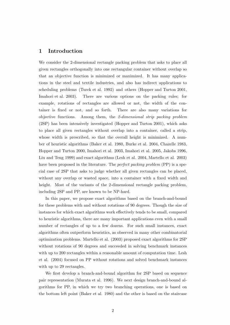
Figure 1: An example of the strip packing problem

2.1 The strip packing problem

Let I = {1, 2, . . . , n} be a set of n rectangles. We are given a width wi and a

height hi for each rectangle i ∈ I and a width W of the strip. The strip packing

problem is to place n rectangles without overlap into the strip so as to minimize

the height H of the strip. Designate the bottom left corner of the strip as the

origin of the xy-plane, letting the x-axis be the direction of the width of the strip,

and the y-axis be the direction of the height. We represent the location of each

3

rectangle i in the strip by the coordinate (xi, yi) of its bottom left corner (see

Fig. 1). The set of coordinates π = {(xi, yi) | i ∈ I ′} for a subset I ′ of I is called

a placement of I ′. Then the strip packing problem is formulated as follows:

minimize H

subject to xi + wi ≤ W, ∀i ∈ I

yi + hi ≤ H, ∀i ∈ I

xi + wi ≤ xj or xj + wj ≤ xi or

yi + hi ≤ yj or yj + hj ≤ yi,∀i, j ∈ I, i �= j

xi, yi ≥ 0, ∀i ∈ I,

where the strip width W is a given constant, while the height H is a variable.

The first, second and last constraints require that all rectangles are in the strip

with width W and height H. The third prevents rectangles from overlapping

each other. A placement π = {(xi, yi) | i ∈ I} of I is called feasible if it satisfies

the above constraints.

In this paper, all widths and heights of rectangles and the strip are assumed

to be integers.

2.2 The perfect packing problem

Given a width wi and a height hi for each rectangle i ∈ I and a width W

and a height H of the container, the perfect packing problem is to determine

whether all given n rectangles can be placed into the container without overlap

and wasted space, and to output a feasible solution if the answer is yes. The

equation∑

i∈I wihi = WH is obviously required to hold so that PP is feasible.

The perfect packing problem is also considered as a problem of judging whether

the optimal value H for the strip packing problem is equal to an obvious lower

bound∑

i∈I wihi/W .

3 Branch-and-bound method

The branch-and-bound method is known as one of the representative method-

ologies for designing exact algorithms for combinatorial optimization problems

(Ibaraki 1987, Lesh et al. 2004, Martello et al. 2003). It is based on the idea

that a problem instance can be solved by dividing it into some partial problem

instances and solving all of them. The operation of dividing a problem instance

is called a branching operation.

We denote by P0 the original problem instance and by Pk the kth partial

problem instance generated during computation. For example, a partial problem

4

for 2SP is defined by a subset I ′ of the entire rectangle set I together with a place-

ment πI′ of I ′, and asks to find a feasible placement πI\I′ of I \ I ′ that minimizes

height H. The process of applying branching operations can be expressed by a

search tree, whose root corresponds to P0, and the children of a node correspond

to the partial problems generated by a branching operation applied to the node.

Each node of in the search tree corresponds to a partial problem instance. For

example, a branching operation chooses each rectangle i from the set I \ I ′ of the

remaining rectangles and adds it to I ′. If an optimal solution to Pk is found or it

is concluded for some reason that we can obtain an optimal solution to P0 even

without solving Pk or that Pk is infeasible, then it is not necessary to consider

Pk further. The operation of removing such a Pk from a list of partial problem

instances to be solved is called a bounding operation; we say that this operation

terminates Pk. For example, when a partial problem Pk is generated by adding

a last rectangle {i} = I \ I ′ and finding a placement for I ′ ∪ {i} = I, we do not

need divide Pk any more.

A partial problem instance is called active if it has been neither terminated nor

divided into partial problem instances. When no active partial problem instance

is left, a branch-and-bound algorithm terminates and delivers an exact optimal

solution.

In the next section, we construct a branch-and-bound algorithm for 2SP such

that branching operations fix relative positions of rectangles in a subset I ′ ⊆ I of

partial problem Pk. Then a single run of the algorithm gives an optimal solution of

the instance. In Section 5, we construct a branch-and-bound algorithm for PP in

which branching operations fix absolute positions of rectangles in a subset I ′ ⊆ I

of partial problem Pk. We then apply it to 2SP in Section 6. An optimal solution

of 2SP will be searched by fixing height H as constants repeatedly in order to

apply the branch-and-bound algorithm for PP, which is a decision problem.

4 Branch-and-bound algorithm based on the se-

quence pair

This section presents a branch-and-bound algorithm based on the sequence pair.

For simplicity, we mainly focus on the case of 2SP without rotations. To repre-

sent relative positions of rectangles, Murata et al. introduced the sequence pair

(Murata et al. 1996), which is defined as a pair of permutations σ = (σ+, σ−) of

the set I = {1, 2, . . . , n}, where σ+(l) = i (equivalently σ−1+ (i) = l) means that

the lth rectangle in σ+ is i, and the definition of σ−(l) is similar. A sequence pair

5

σ = (σ+, σ−) defines the following two partial orders �xσ and �y

σ on I:

σ−1+ (i)≤σ−1

+ (j) and σ−1− (i)≤σ−1

− (j) ⇐⇒ i �xσ j,

σ−1+ (i)≥σ−1

+ (j) and σ−1− (i)≤σ−1

− (j) ⇐⇒ i �yσ j.

For a given σ, let Πσ be the set of placements {(xi, yi) | i ∈ I} that satisfy the

following conditions:

i �xσ j and i �= j =⇒ xi + wi ≤ xj ,

i �yσ j and i �= j =⇒ yi + hi ≤ yj .

Given a sequence pair σ, exactly one of the four relations i �xσ j, j �x

σ i, i �yσ j

and j �yσ i holds for arbitrary i and j with i �= j, and therefore any two rectangles

in I never overlap each other in any placement in Πσ. For sequence pairs, the

following lemma is known.

Lemma 1 (Imahori et al. 2003, Murata et al. 1996) For a given sequence pair σ

on I, an optimal placement {(xi, yi) | i ∈ I} ∈ Πσ that minimizes simultaneously

both xmax = maxi∈I(xi + wi) and ymax = maxi∈I(yi + hi) can be computed in

time polynomial in |I|. Conversely, for any feasible placement π of I, there exists

a sequence pair σ on I that satisfies π ∈ Πσ.

This lemma means that an optimal solution is guaranteed to be contained

certainly in the set Πσ for some σ. Then we only have to consider how to find

such a σ using branch-and-bound. We now explain nodes, the branching rule,

the bounding rule and search strategy in our branch-and-bound based on the

sequence pairs, which we call ‘BB-SP.’

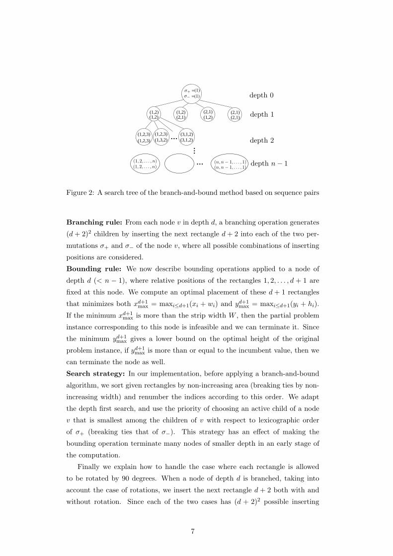
Nodes: Each node of depth d in the search tree corresponds to a partial problem

instance which is defined by fixing relative positions of the rectangles 1, 2, . . . , d+

1. The root node represents the set Πσ of placements for sequence pair σ = (σ+ =

(1), σ− = (1)) on {1}, and each node of depth d represents Πσ for a sequence pair

σ = (σ+, σ−) on the set of the first d + 1 rectangles {1, 2, . . . , d + 1}. The nodes

of depth n − 1 are leaves of the search tree and represent Πσ for sequence pairs

σ = (σ+, σ−) on I = {1, 2, . . . , n}. Hence, the search tree has at most ((d + 1)!)2

nodes of depth d for each d = 0, 1, . . . , n−1. See an example in Fig. 2, where each

node shown as a circle has two permutations: the upper permutation represents

σ+ and the lower σ−.

6

=(1)=(1)

(2,1)(2,1)(2,1)

(1,2) (1,2)(1,2)(1,2) (2,1)

(1,2,3)(1,2,3)

...(1,2,3)(1,3,2)

(3,1,2)(3,1,2)

...

...

σ+

σ− depth 0

depth 1

depth 2

depth n − 1(1, 2, . . . , n)(1, 2, . . . , n)

(n, n − 1, . . . , 1)(n, n − 1, . . . , 1)

Figure 2: A search tree of the branch-and-bound method based on sequence pairs

Branching rule: From each node v in depth d, a branching operation generates

(d + 2)2 children by inserting the next rectangle d + 2 into each of the two per-

mutations σ+ and σ− of the node v, where all possible combinations of inserting

positions are considered.

Bounding rule: We now describe bounding operations applied to a node of

depth d (< n − 1), where relative positions of the rectangles 1, 2, . . . , d + 1 are

fixed at this node. We compute an optimal placement of these d + 1 rectangles

that minimizes both xd+1max = maxi≤d+1(xi + wi) and yd+1

max = maxi≤d+1(yi + hi).

If the minimum xd+1max is more than the strip width W , then the partial problem

instance corresponding to this node is infeasible and we can terminate it. Since

the minimum yd+1max gives a lower bound on the optimal height of the original

problem instance, if yd+1max is more than or equal to the incumbent value, then we

can terminate the node as well.

Search strategy: In our implementation, before applying a branch-and-bound

algorithm, we sort given rectangles by non-increasing area (breaking ties by non-

increasing width) and renumber the indices according to this order. We adapt

the depth first search, and use the priority of choosing an active child of a node

v that is smallest among the children of v with respect to lexicographic order

of σ+ (breaking ties that of σ−). This strategy has an effect of making the

bounding operation terminate many nodes of smaller depth in an early stage of

the computation.

Finally we explain how to handle the case where each rectangle is allowed

to be rotated by 90 degrees. When a node of depth d is branched, taking into

account the case of rotations, we insert the next rectangle d + 2 both with and

without rotation. Since each of the two cases has (d + 2)2 possible inserting

7

positions, we generate 2(d + 2)2 children of depth d + 1. The other parts of the

algorithm are designed in the same manner as those without rotations.

5 Branch-and-bound algorithm for PP

In this section, we first focus on PP and consider another type of branch-and-

bound algorithms based on the framework of algorithms described in Section 5.1.

For PP, height H of the container is fixed to∑

wihi/W . This algorithm performs

branching operations by fixing absolute positions (coordinates) of rectangles one

by one as it goes down in the search tree. We first describe nodes, branching

rules, bounding rules and search strategy in our branch-and-bound algorithm for

PP. Details of branching rules and bounding rules are explained in Sections 5.2

and 5.3, respectively.

Nodes: The root node represents the empty container, and a node of depth d

represents a subset I ′ ⊆ I of d rectangles together with absolute positions of the

d rectangles.

Branching rules: A branching operation at a node of depth d for I ′ ⊆ I

corresponds to choosing a rectangle r ∈ I \ I ′ and placing the rectangle r in the

open space of the current placement based on some rule.

Bounding rules: As PP is a decision problem, if we find out that a partial prob-

lem for I ′ ⊆ I does not have a perfect packing by placing the remaining rectangles

in I \ I ′, then we terminate the corresponding node, and if we obtain a perfect

packing at a leaf node, then we can terminate the entire search immediately and

the answer is yes.

Search strategy: Before applying a branch-and-bound algorithm, we sort given

rectangles by non-increasing area (breaking ties by non-increasing width) and

renumber the indices according to this order. When we perform a branching

operation, we add the generated nodes to a list A of active nodes in the decreasing

order of indices of the lastly placed rectangles. We adapt the depth first search.

That is, when we perform a branching operation for an active nodes, we choose

the newest one, in which the the least indexed rectangle is lastly placed, from

the list A. We confirm through preliminary experiments that this adding order

is effective for most of the instances.

5.1 Algorithm BB-PP

The entire framework of the branch-and-bound algorithm for PP, called algorithm

BB-PP, is formally described as follows, where A is the set of active nodes.

8

Algorithm BB-PP

Step 0 (initialization). Sort a given set I of rectangles in the order of non-

increasing areas (breaking ties by non-increasing width) and renumber the

indices according to this order. Let A := {the original instance} and I ′ :=

∅.

Step 1 (judgement). If the set A is empty, then output ‘infeasible’ and stop.

Otherwise choose the newest node u from A and let A := A \ {u}, adapting

the depth first search. If the placement πu is a perfect packing, then output

‘feasible’ and stop.

Step 2 (bounding operation). Apply the bounding rules in Section 5.3 to the

placement πu. If u is terminated, return to Step 1. (Not necessarily all

bounding rules are used. We examine various combinations in Section 7.)

Step 3 (branching operation). If I \ I ′ �= ∅, then generate the children of

u based on a branching rule in Section 5.2 (BL placement or staircase

placement), I ′ := I ′ ∪ {the placed rectangle}, and add these nodes to A in

the decreasing order of indices of the placed rectangles. (This means that

the child branched with the least indexed rectangle will be searched next.)

Return to Step 1.

5.2 Branching rules

We consider two branching rules, one is based on the bottom left point and the

other based on the staircase placement, which will be explained in Sections 5.2.1

and 5.2.2, respectively. Let B = [0, W ] × [0, H] denote the set of all points

inside or on the boundary of the container. For a subset I ′ ⊆ I, a placement

of I ′ is defined by π = {(xi, yi) | i ∈ I ′}. For a given placement π of I ′, let

Cπ = {(x, y) | xi ≤ x ≤ xi + wi and yi ≤ y ≤ yi + hi for some i ∈ I ′} denote the

set of points inside the placed rectangles or on their boundaries. Let Uπ = B\Cπ,

and cl(Uπ) denote the closure of Uπ, i.e., the minimum closed set including Uπ

(see Fig. 3(a)).

5.2.1 Branching based on the bottom left point

We first explain the branching based on the bottom left placement for the case

without rotations. The leftmost point in the lowest positions of cl(Uπ) is called

the BL point (Baker et al. 1980). For example, Fig. 3(a) shows the BL point

9

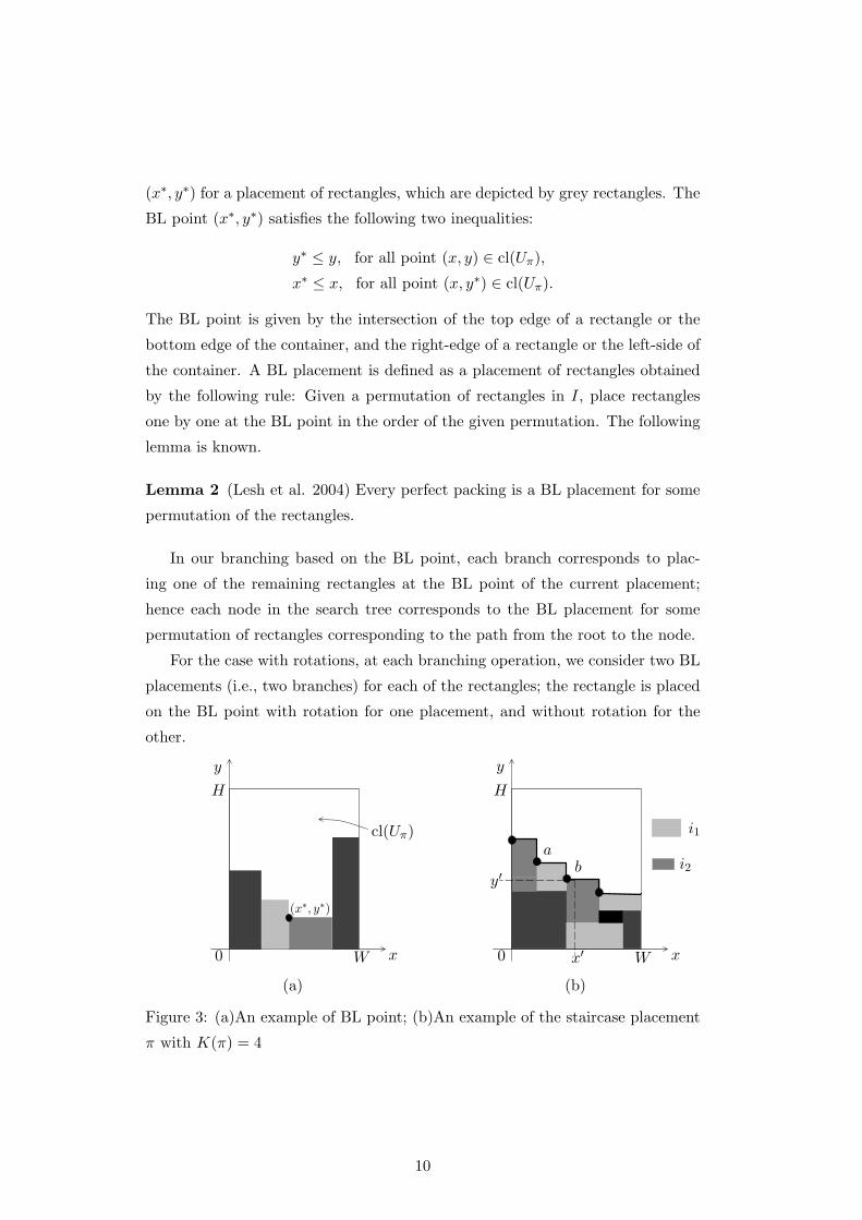
(x∗, y∗) for a placement of rectangles, which are depicted by grey rectangles. The

BL point (x∗, y∗) satisfies the following two inequalities:

y∗ ≤ y, for all point (x, y) ∈ cl(Uπ),

x∗ ≤ x, for all point (x, y∗) ∈ cl(Uπ).

The BL point is given by the intersection of the top edge of a rectangle or the

bottom edge of the container, and the right-edge of a rectangle or the left-side of

the container. A BL placement is defined as a placement of rectangles obtained

by the following rule: Given a permutation of rectangles in I, place rectangles

one by one at the BL point in the order of the given permutation. The following

lemma is known.

Lemma 2 (Lesh et al. 2004) Every perfect packing is a BL placement for some

permutation of the rectangles.

In our branching based on the BL point, each branch corresponds to plac-

ing one of the remaining rectangles at the BL point of the current placement;

hence each node in the search tree corresponds to the BL placement for some

permutation of rectangles corresponding to the path from the root to the node.

For the case with rotations, at each branching operation, we consider two BL

placements (i.e., two branches) for each of the rectangles; the rectangle is placed

on the BL point with rotation for one placement, and without rotation for the

other.

0 x

y

W

H

(x∗, y∗)

cl(Uπ)

(a)

0 x

y

W

H

x′

y′

ab

i1

i2

(b)

Figure 3: (a)An example of BL point; (b)An example of the staircase placement

π with K(π) = 4

10

5.2.2 Branching based on the staircase placement

A placement π = {(xi, yi) | i ∈ I ′} for a subset I ′ ⊆ I of rectangles, is called

a staircase placement if the following two implications hold for arbitrary points

(x, y) ∈ Cπ and (x′, y′) ∈ Uπ:

y = y′ ⇒ x ≤ x′, (5.1)

x = x′ ⇒ y ≤ y′ (5.2)

(see Fig. 3(b)). In other words, in a staircase placement, the boundary between

Cπ and Uπ forms a monotone (right-down) staircase, and the space below the

boundary is filled with placed rectangles without wasted space. The leftmost

points of the horizontal lines of the boundary (the four dots in Fig. 3(b)) are

called corner points. For a staircase placement π, we define the number of the

corner points on the staircase as the number of stairs K(π). We perform branch-

ing operations by placing rectangles at corner points, keeping the placement as a

staircase placement. Therefore, in the search tree based on this branching oper-

ation, a node v is a child of a node u if and only if v corresponds to a staircase

placement πv that is obtainable by placing one of the remaining rectangles at a

corner point of the placement πu of u. It is not difficult to see that the correctness

of this branching operation is derived from the following lemma:

Lemma 3 For any staircase placement with at least one rectangle, there exists a

rectangle such that the two conditions (5.1) and (5.2) hold even after its removal.

Since the number of stairs K(π) is less than or equal to �n/2 for any staircase

placement obtained from a perfect packing of I by Lemma 3, we do not generate

any placement such that the number of stairs is more than �n/2 . The idea of

using staircase placements was first proposed by Martello el al. (2000) in a more

general form for 2SP.

In the case of PP with rotations, we consider placements of each rectangle

both with and without rotation at the corner points.

Limitation on the number of stairs

Perfect placements sometimes consist of several compound rectangles, and such

placements do not need many stairs to place rectangles with the staircase place-

ment strategy. To find such placements more quickly, we introduce the following

heuristic rule. We set an upper limit κ on the number of stairs during the search;

i.e., if a generated node corresponds to a staircase placement π whose number

11

of stairs K(π) > κ, then we terminate the node immediately. This heuristic

rule often finds a feasible solution more quickly if a given instance is feasible

(Matsuda 1998). We first set κ = 2. If the search terminates all active nodes

without finding a feasible placement with the current limit κ, then we increase

the limit by one. We repeat this process until κ becomes 4. If we cannot find a

feasible solution with κ = 4, we increase limit κ to �n/2 , which is equivalent to

the case with no limitation on K(π). If no feasible solution is found even with

κ = �n/2 , then we conclude that the instance is infeasible.

Redundancy check

Branching based on the staircase placement may generate two nodes u, v which

correspond to the same placement πu = πv. For example, consider two corner

points a, b of a placement π for I ′ ⊆ I and two rectangles i1, i2 ∈ I \ I ′ (see

Fig. 3(b)). The node u generated by placing rectangle i1 at a after placing

rectangle i2 at b and the node v generated by placing rectangle i2 at b after

placing rectangle i1 at a are descendants of the node for I ′, and have the same

placement πu = πv. It is difficult to avoid this redundancy completely during

computation. We explain some technique to reduce such redundancy.

For each rectangle r ∈ I, we introduce a list Lr that stores the positions

already searched, and check the list whenever we place the rectangle r. This

technique is also used by Martello et al. (2003), but we extend it so as to share

the lists among all rectangles of the same shape. If there are rectangles i and j

whose shapes are same (i.e., wi = wj and hi = hj), then they share the same list.

This is especially effective when we treat many rectangles with the same shapes.

Moreover, we maintain another list that stores all the searched placements

with a small number of stairs (at most two stairs). We check the list whenever

the number of stairs K(π) of the placement πv of the current node v for I ′ ⊆ I

is less than or equal to two to avoid a redundant search. If the list contains a

placement π for some I ′′ ⊆ I such that all the coordinates of corner points of π

and πv are the same, and I ′′ = I ′, then we terminate search for the descendants

of v.

5.3 Bounding operations

This subsection describes our three rules for bounding operations, dynamic pro-

gramming cut (DP cut), the bounding rule based on the staircase placement and

the remaining rectangles, and LP cut, which will be explained in Sections 5.3.1,

5.3.2 and 5.3.3 respectively.

12

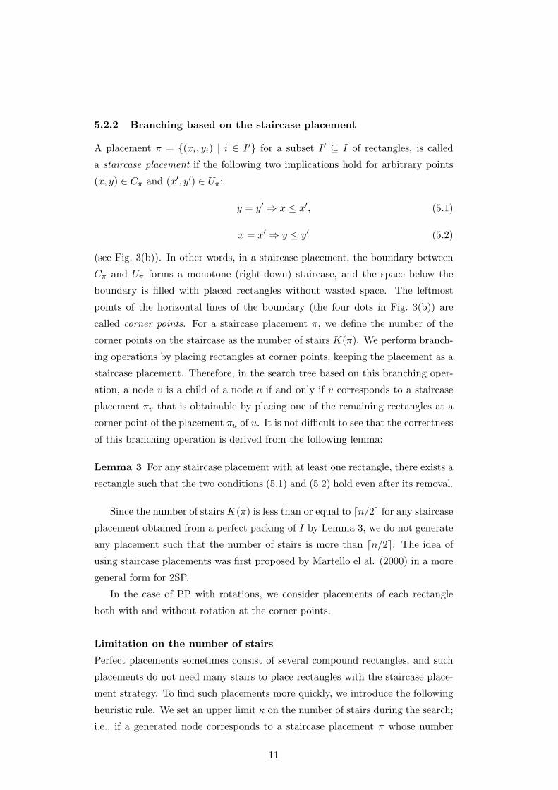
5.3.1 Dynamic programming cut (DP cut)

This subsection introduces DP cut. For a placement π of some subset I ′ ⊂ I of

rectangles, there are vertical gaps between the top of the container and upper

edges of rectangles, and horizontal gaps between the side edges of rectangles or

one of the sides of the container (Fig. 4). All such gaps should be filled with the

remaining rectangles in I \ I ′ so that a perfect packing for I is obtained. To be

more precise, a vertical (resp., horizontal) gap is the length of a vertical (resp.,

horizontal) line segment that satisfies the following three conditions:

(1) Any point on the line segment is in cl(Uπ).

(2) Both end points of the line segment are on the boundary of cl(Uπ).

(3) Other points on the line segment are not on the boundary of cl(Uπ).

If there is a gap that cannot be realized by any combination of the lengths of the

remaining rectangles I \I ′ , then we can terminate the node for π since no perfect

packing can be constructed by extending the current placement π. We call this

bounding rule DP cut and use this in both branching rules with Sections 5.2.1

and 5.2.2.

0 x

y

W

H

Figure 4: An example of vertical and horizontal gaps for a placement π

We compute whether each of the gaps can be realized by a combination of the

lengths, wi, hi, i ∈ I \I ′, as follows. We first consider the case with rotations. For

a given placement π = {(xi, yi) | i ∈ I ′}, we denote the remaining rectangles in

I\I ′ by i = 1, 2, . . . , m for simplicity. The problem of judging whether a given gap

can be filled is formulated as a problem similar to the subset sum problem, and

it can be solved by using dynamic programming (DP) (Martello and Toth 1990).

Let zri (resp., zu

i ) be a 0,1-variable that takes value 1 if we use the rotated (resp.,

13

unrotated) rectangle i to fill the gap, and 0 otherwise. Then, for t = 1, 2, . . . , m

and an integer p ≥ 0, the problem Qt(p) of finding a combination of rectangles

from {1, 2, . . . , t} that realizes vertical gap p ≥ 0 is formally described as follows:

Qt(p) Find z = (zr1, z

r2, . . . , z

rt , z

u1 , zu

2 , . . . , zut )

such thatt∑

i=1

(wizri + hiz

ui ) = p

zri + zu

i ≤ 1, ∀i = 1, 2, . . . , t

zri , z

ui ∈ {0, 1}, ∀i = 1, 2, . . . , t.

(Note that, though our objective is to find a solution to Qm(p), we define the

problem for all t ≤ m for convenience.) Let vt(p) be 1 if there exists a solution

to Qt(p) and 0 otherwise. That is, it is a possible to fill a gap with length p if

and only if vm(p) = 1.

Lemma 4 All vt(p), t = 1, 2, . . . , m can be computed in O(m(W + H)) time.

Proof. We can compute vt(p) by

v0(p) =

⎧⎨⎩

1, p = 0,

0, otherwise,(5.3)

vt(p) = max{vt−1(p), vt−1(p − wt), vt−1(p − ht)}, (5.4)

t = 1, 2, . . . , m,

where v0(p) are boundary conditions that represent trivial cases with the empty

set of rectangles. Note that vt(p) = 0 holds for any p < 0 by the definition.

Note that a single run of the above algorithm suffices to find the feasibility

of all vertical gaps. The same algorithm can also judge the feasibility of horizon-

tal gaps just by exchanging the roles of variables zr1 and zn

i . We can therefore

compute the feasibility of all vertical and horizontal gaps by only one run of the

above DP recursion. Though we define vt(p) for all nonnegative integers p, we

need to calculate it only for p = 0, 1, . . . ,max {W, H}; hence the above recurrence

formula can be calculated in O(m(W + H)) time.

In the case of the problem without rotations, the problem becomes equivalent

to the subset sum problem, and we only need to execute similar DPs for the

horizontal and vertical gaps independently. When we calculate the DP for the

vertical (resp., horizontal) gaps, we remove the second term vt−1(p − wt) (resp.,

the third term vt−1(p − ht)) from the recurrence formula (5.4).

A similar idea is also used in (Lesh et al. 2004), where only horizontal gaps

are considered and upper bounds on the possible height of the gap is computed

14

based on a slightly more complicated DP recursion. We simplify their DP, not

considering the height but using 0,1-variables, in order to apply it to the case

with rotations.

Adaptive control of DP cut

We observed through preliminary experiments that DP cut often fails in termi-

nating nodes especially when the depth of the node in the search tree is relatively

small. Since executing DP cut is expensive, we incorporate a mechanism to con-

trol timing of invoking the DP cut procedure. For this, we use a variable β. We

invoke DP cut only if the depth d of the current node satisfies d ≥ β. We control

the variable β using two constant parameters δ and q as follows. We set β = 0

at the root node. Whenever we succeed in terminating a node by a DP cut,

we reduce β to max{β − δ, 0}. When the DP cut procedure fails in terminating

nodes q consecutive times, we increase β by 1. We use δ = 1 and q = 4 in the

computational experiments in Section 7.

5.3.2 The bounding rule based on the staircase placement and the

remaining rectangles

We introduce three simple bounding rules, which are applicable only in the

branching based on the staircase placement. (I) If the number of the remain-

ing rectangles |I \ I ′| becomes smaller than the number of corner points of π in a

node, then we terminate the node immediately since it is impossible to construct

a perfect packing of I by extending π. (II) If we find a rectangle r in I \ I ′ which

cannot be placed at any corner point of the staircase of π without protruding

from the container, then we terminate the node immediately. (III) If all the in-

dices of the remaining rectangles becomes smaller than the index of the rectangle

placed at the origin (0, 0), then we terminate the node immediately since we have

judged all possible placement in cl(Uπ) are infeasible in corresponding placement

with rotation of 180 degrees.

5.3.3 LP cut

Formulating PP as an integer programming problem, we consider a bounding

operation based on its linear programming (LP) relaxation. This operation is

applicable to both branching strategies in Sections 5.2.1 and 5.2.2.

We first explain the case with rotations. We define variables z+i,x,y and z−i,x,y

for i ∈ I and (x, y) ∈ B = {0, 1, . . . , W} × {0, 1, . . . , H}, where their meanings

15

are as follows:

• z+i,x,y = 1 if rectangle i is placed at (x, y) without rotation, and 0 otherwise.

• z−i,x,y = 1 if rectangle i is placed at (x, y) with rotation, and 0 otherwise.

Moreover, we define B+i = {(x, y) | x = 0, 1, . . . , W − wi, y = 0, 1, . . . , H − hi}

and B−i = {(x, y) | x = 0, 1, . . . , W − hi, y = 0, 1, . . . , H − wi} for each i ∈ I.

Then PP can be formulated as the following integer program:

maximize∑i∈I

∑(x,y)∈B+

i

z+i,x,y +

∑i∈I

∑(x,y)∈B−

i

z−i,x,y

subject to∑

(x,y)∈B+i

z+i,x,y +

∑(x,y)∈B−

i

z−i,x,y ≤ 1 , ∀i ∈ I

∑i∈I

∑x−wi<x′≤xy−hi<y′≤y

z+i,x′,y′+

∑i∈I

∑x−hi<x′≤xy−wi<y′≤y

z−i,x′,y′ ≤1 , ∀(x, y) ∈ B

z+i,x,y, z

−i,x,y ∈ {0, 1} , ∀i ∈ I, (x, y) ∈ B

z+i,x,y = 0 , ∀i ∈ I, (x, y) /∈ B+

i

z−i,x,y = 0 , ∀i ∈ I, (x, y) /∈ B−i .

The first constraint means that each rectangle cannot be placed more than once

and the second means that no rectangles overlap each other. The original instance

for PP has a perfect packing if and only if the optimal value of the corresponding

instance of this problem is equal to n.

We now consider the LP relaxation of this problem by relaxing constraints

z+i,x,y, z

−i,x,y ∈ {0, 1} to 0 ≤ z+

i,x,y, z−i,x,y ≤ 1 for all i ∈ I and (x, y) ∈ B.

Lemma 5 For a given placement π = {(xi, yi) | i ∈ I ′} of rectangles, the vari-

ables z+i,x,y, z

−i,x,y corresponding to the placed rectangles i ∈ I ′ are fixed, and if

the optimal value of the corresponding LP instance is less than n, then no perfect

packing of I exists by extending π.

This formulation contains Ω(nWH) variables and WH+n constraints. Hence

this bounding rule is not practical for problem instances with relatively large WH.

We can also treat an LP relaxation for the case without rotations. In this

case, variables z−i,x,y are fixed to 0, and thus not necessarily introduced in this

formulation.

6 Application to general 2SP

This section gives some ideas to apply our algorithms in the previous section

to general 2SP. We first explain how to reduce 2SP to PP in Section 6.1, and

16

introduce generalizations of staircase placement, DP cut, and the bounding rule

based on the staircase placement and the remaining rectangles in Sections 6.2,

6.3 and 6.3.1. We then introduce our two algorithms for 2SP in Section 6.4.

6.1 Reduction from 2SP to PP

For a given 2SP instance with a set I of rectangles, let H ′ be an integer such that

WH ′ ≥ ∑i∈I wihi. The optimal value of the 2SP instance is less than or equal

to H ′ if and only if the following PP instance is feasible. We set the height of

the container to H ′, and add WH ′ − ∑i wihi new 1 × 1 rectangles to the set I

so that equation∑

wihi = WH ′ holds for the resulting instance, where “1 × 1”

means that its height and width are 1.

Since we assume that all widths and heights of rectangles are integers, the

optimal value of 2SP is also an integer. Hence, 2SP is equivalent to determining

the minimum H ′ such that the corresponding PP instance has a perfect packing.

6.2 Generalizations of staircase placement

We explain a generalization of staircase placement. The idea of adding 1 × 1

rectangles is less effective if we need to add many 1 × 1 rectangles. We therefore

consider another idea that does not require to handle 1×1 rectangles explicitly. To

find a perfect placement, the space below the boundary in a placement π of a node

in a search tree must be filled with placed rectangles without wasted space in the

staircase placement in Section 5.2.2. In this section, we generalize the definition

of the staircase placement so that it allows wasted space in the space below the

boundary of placements π. We modify the definition of staircase in Section 5.2.2

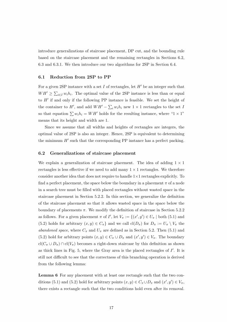
as follows. For a given placement π of I ′, let Vπ := {(x′, y′) ∈ Uπ | both (5.1) and

(5.2) holds for arbitrary (x, y) ∈ Cπ} and we call cl(Dπ) for Dπ := Uπ \ Vπ the

abandoned space, where Cπ and Uπ are defined as in Section 5.2. Then (5.1) and

(5.2) hold for arbitrary points (x, y) ∈ Cπ ∪ Dπ and (x′, y′) ∈ Vπ. The boundary

cl(Cπ ∪ Dπ) ∩ cl(Vπ) becomes a right-down staircase by this definition as shown

as thick lines in Fig. 5, where the Gray area is the placed rectangles of I ′. It is

still not difficult to see that the correctness of this branching operation is derived

from the following lemma:

Lemma 6 For any placement with at least one rectangle such that the two con-

ditions (5.1) and (5.2) hold for arbitrary points (x, y) ∈ Cπ∪Dπ and (x′, y′) ∈ Vπ,

there exists a rectangle such that the two conditions hold even after its removal.

17

As in the branching operation based on the original staircase placement, we do

not fill the space below the boundary in the descendants of the search tree. Thus,

we perform branching operations by placing rectangles at the corner points of the

staircase. Let the number of stairs K(π) denote the number of corner points. The

validity of this branching operation is proved in (Martello et al. 2000).

0 x

y

W

H

Vπ

Dπ

Figure 5: Generalized definition of staircase

6.3 Extension of DP cut

DP cut can be applied directly to 2SP if we adapt the strategy in Section 6.1; i.e.,

we calculate DP after adding 1 × 1 rectangles. However, as the number of 1 × 1

rectangles increases, gaps become easier to be realized and the DP cut becomes

less effective to terminate nodes. To alleviate this, we propose a new idea of

executing the DP computation without 1 × 1 rectangles explicitly. For a given

placement π of I ′, let gvk (resp., gh

k) be the length of the kth shortest vertical

gap (resp., the kth longest horizontal gap ghk) in π (k = 1, 2, . . . , K(π)), and sh

k

(resp., svk) be the width (resp., height) of the stair which forms the boundary of

the gap in π (see Fig. 6(a)). Let J be a subset of I \ I ′. We then compute lvk

(resp., lhk), the maximum realizable length by some combination of the lengths of

the rectangles in J less than or equal to gvk (resp., gh

k). Then shk(gv

k − lvk) (resp.,

svk(g

hk − lhk)) gives a lower bound on the area in Vπ that cannot be filled with

any combination of rectangles in J . When we sum such areas shk(gv

k − lvk) over

all vertical gaps and svk(g

hk − lhk) over all horizontal gaps, we need to subtract

the common area (gvk − lvk)(gh

k − lhk) since the space is doubly added. Moreover,

(gvk − lvk)(gh

k+1 − lhk+1), k = 1, 2, . . . , K(π) − 1 gives another area that cannot be

filled with rectangles in J . We show that the total of these area, which is depicted

as a dark gray area of Fig. 6(b), is a lower bound on the area in Vπ that cannot

18

be filled with any combination of the rectangles in J .

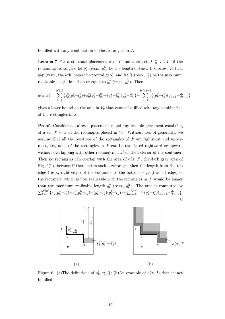
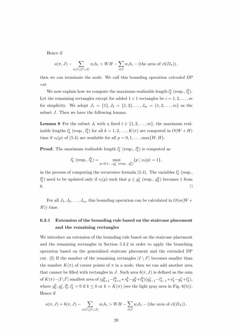
Lemma 7 For a staircase placement π of I ′ and a subset J ⊆ I \ I ′ of the

remaining rectangles, let gvk (resp., gh

k) be the length of the kth shortest vertical

gap (resp., the kth longest horizontal gap), and let lvk (resp., lhk) be the maximum

realizable length less than or equal to gvk (resp., gh

k). Then

a(π, J) =K(π)∑k=1

{shk(gv

k−lvk)+svk(g

hk−lhk)−(gv

k−lvk)(ghk−lhk)}+

K(π)−1∑k=1

{(gvk−lvk)(gh

k+1−lhk+1)}

gives a lower bound on the area in Vπ that cannot be filled with any combination

of the rectangles in J .

Proof. Consider a staircase placement π and any feasible placement consisting

of a set J ′ ⊆ J of the rectangles placed in Vπ. Without loss of generality, we

assume that all the positions of the rectangles of J ′ are rightmost and upper-

most, i.e., none of the rectangles in J ′ can be translated rightward or upward

without overlapping with other rectangles in J ′ or the exterior of the container.

Then no rectangles can overlap with the area of a(π, J), the dark gray area of

Fig. 6(b), because if there exists such a rectangle, then the length from the top

edge (resp., right edge) of the container to the bottom edge (the left edge) of

the rectangle, which is now realizable with the rectangles in J , would be longer

than the maximum realizable length gvk (resp., gh

k). The area is computed by∑K(π)k=1 {sh

k(gvk−lvk)+sv

k(ghk−lhk)−(gv

k−lvk)(ghk−lhk)}+∑K(π)−1

k=1 {(gvk−lvk)(gh

k+1−lhk+1)}.

1

2

3

sv2 sh

2

gv3 lv3

sh3(g

v3 − lv3)

π

(a)

1

2

3πa(π, J)

(b)

Figure 6: (a)The definitions of shk, gv

k , lvk; (b)An example of a(π, J) that cannot

be filled

19

Hence if

a(π, J) −∑

i∈I\(I′∪J)

wihi > WH −∑i∈I

wihi − (the area of cl(Dπ)) ,

then we can terminate the node. We call this bounding operation extended DP

cut.

We now explain how we compute the maximum realizable length lvk (resp., lhk).

Let the remaining rectangles except for added 1× 1 rectangles be i = 1, 2, . . . , m

for simplicity. We adopt J1 = {1}, J2 = {1, 2}, . . . , Jm = {1, 2, . . . , m} as the

subset J . Then we have the following lemma.

Lemma 8 For the subset Jt with a fixed t ∈ {1, 2, . . . , m}, the maximum real-

izable lengths lvk (resp., lhk) for all k = 1, 2, . . . , K(π) are computed in O(W + H)

time if vt(p) of (5.4) are available for all p = 0, 1, . . . ,max{W, H}.

Proof. The maximum realizable length lvk (resp., lhk) is computed as

lvk (resp., lhk) = maxp=0,1,...,gv

k(resp., gh

k){p | vt(p) = 1},

in the process of computing the recurrence formula (5.4). The variables lvk (resp.,

lhk) need to be updated only if vt(p) such that p ≤ gvk (resp., gh

k) becomes 1 from

0.

For all J1, J2, . . . , Jm, this bounding operation can be calculated in O(m(W +

H)) time.

6.3.1 Extension of the bounding rule based on the staircase placement

and the remaining rectangles

We introduce an extension of the bounding rule based on the staircase placement

and the remaining rectangles in Section 5.3.2 in order to apply the branching

operation based on the generalized staircase placement and the extended DP

cut. (I) If the number of the remaining rectangles |I \ I ′| becomes smaller than

the number K(π) of corner points of π in a node, then we can add another area

that cannot be filled with rectangles in J . Such area b(π, J) is defined as the sum

of K(π)−|I\I ′| smallest area of (ghk+1−lhk+1+sh

k−ghk+lhk)(gv

k−1−lvk−1+svk−gv

k+lvk),

where ghk , gv

k , lhk , lvk = 0 if k ≤ 0 or k > K(π) (see the light gray area in Fig. 6(b)).

Hence if

a(π, J) + b(π, J) −∑

i∈I\(I′∪J)

wihi > WH −∑i∈I

wihi − (the area of cl(Dπ)) ,

20

then we can terminate the node. (II) and (III) can be applied directly. We call

these bounding operations extended bounding rule based on the staircase place-

ment and the remaining rectangles.

6.4 Algorithms

We propose two algorithms for 2SP; one uses branching operations based on the

staircase placement in Section 5.2.2 and adds 1 × 1 rectangles, and the other

uses branching operations based on the generalized staircase placement in Sec-

tion 6.2 without adding 1×1 rectangles explicitly. We call the resulting algorithms

STAIRCASE and G-STAIRCASE, respectively. These two algorithms adapt the

extended DP cut in Section 6.3 and the extended bounding rule based on the

staircase placement and the remaining rectangles in Section 6.3.1 as their bound-

ing operations. We observed through computational experiments that LP cut in

Section 5.3.3 is not effective for these algorithms (see Section 7.3.1).

Algorithm STAIRCASE

We first compute a lower bound LB on the optimal height by

LB = min{⌈∑

i∈I wihi

W

⌉, max

i∈Ihi

}(6.1)

when rotations are not allowed, and by

LB = min{⌈∑

i∈I wihi

W

⌉, max

i∈Imin{hi, wi}

}(6.2)

when rotations are allowed. We then let H := LB and add WH − ∑i∈I wihi

1 × 1 rectangles to the set I to obtain a PP instance. We then test whether the

PP instance is feasible or not using algorithm BB-PP with branching operations

based on the staircase placement in Section 5.2.2. If we find a feasible solution

for the PP instance, then we output the placement as an optimal solution and H

as the optimal value and stop. Otherwise, we increase H by one and repeat this

procedure until a feasible solution is found.

Algorithm G-STAIRCASE

We first compute the same lower bound LB as STAIRCASE and let H := LB.

We then test whether the PP instance is feasible or not using algorithm BB-

PP with branching operations based on the generalized staircase placement in

Section 6.2. If we find a feasible solution for the PP instance, then we output

the placement and then stop. Otherwise, we increase H by one and repeat the

procedure until a feasible solution is found.

21

7 Computational results

We first explain the instances that we used. Then we report the computational

results on algorithm BB-SP in Section 4. We next report the computational

results on algorithm BB-PP in Section 5.1 for PP and algorithms STAIRCASE

and G-STAIRCASE in Section 6 for 2SP. In tables, column ‘H∗’ shows optimal

values, column ‘time’ shows the computation time in seconds and column ‘nodes’

shows the number of search tree nodes generated by the algorithm. The mark

‘T.O.’ means that the search did not stop within the time limit. We coded the

algorithms in C language and used a PC with a Pentium 4 (3.0GHz) and 1.0GB

memory for computational experiments of this section.

7.1 Instances

The instances used for our computational experiments are selected as follows. We

use (i) the benchmark instances for PP generated by Hopper, which were used in

(Lesh et al. 2004) and are available at the ESICUP web site1, (ii) the instances

for 2SP, which were used in (Martello et al. 2003) and are available at OR-

Library2 and (iii) the instances generated randomly by Burke et al., which were

used in (Burke et al. 2004) and are available from (Burke et al. 2004). Among

the instances by Hopper, we use the sets N1 (n = 17, W = 200, H = 200),

N2 (n = 25, W = 200, H = 200), N3 (n = 29, W = 200, H = 200), and N4

(n = 49, W = 200, H = 200). Each of N1, N2, N3, and N4 consists of five in-

stances, and those in N1 are named n1a, n1b, . . . , n1e, and those in N2, N3 and

N4 are named similarly. Among the instances in (Martello et al. 2003), we use

the sets ht01–09, beng01–10, cgcut01–03 and ngcut01–12. Among the instances

by Burke, we use the instances n1, n2, . . . , n12.

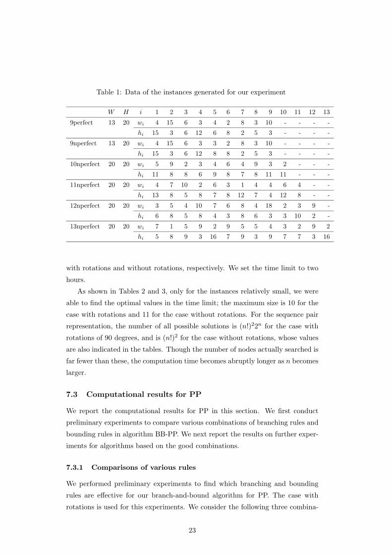
Moreover, we supplemented PP instances with relatively small ones generated

by us. Their data is shown in Table 1. The name of these instances has the

following meanings: ‘perfect’ (resp. ‘nperfect’) means that the instance is feasible

(resp. infeasible) and the number on the left represents the number of rectangles

n.

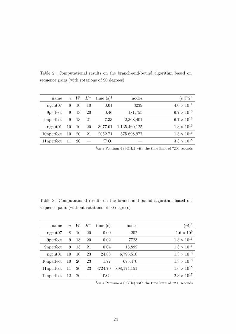
7.2 Computational results on BB-SP

We first report the computational results on BB-SP, the algorithm which is based

on sequence pairs. Tables 2 and 3 show the computational results for the problem

1http://paginas.fe.up.pt/ esicup/2http://www.ms.ic.ac.uk/info.html

22

Table 1: Data of the instances generated for our experiment

W H i 1 2 3 4 5 6 7 8 9 10 11 12 13

9perfect 13 20 wi 4 15 6 3 4 2 8 3 10 - - - -

hi 15 3 6 12 6 8 2 5 3 - - - -

9nperfect 13 20 wi 4 15 6 3 3 2 8 3 10 - - - -

hi 15 3 6 12 8 8 2 5 3 - - - -

10nperfect 20 20 wi 5 9 2 3 4 6 4 9 3 2 - - -

hi 11 8 8 6 9 8 7 8 11 11 - - -

11nperfect 20 20 wi 4 7 10 2 6 3 1 4 4 6 4 - -

hi 13 8 5 8 7 8 12 7 4 12 8 - -

12nperfect 20 20 wi 3 5 4 10 7 6 8 4 18 2 3 9 -

hi 6 8 5 8 4 3 8 6 3 3 10 2 -

13nperfect 20 20 wi 7 1 5 9 2 9 5 5 4 3 2 9 2

hi 5 8 9 3 16 7 9 3 9 7 7 3 16

with rotations and without rotations, respectively. We set the time limit to two

hours.

As shown in Tables 2 and 3, only for the instances relatively small, we were

able to find the optimal values in the time limit; the maximum size is 10 for the

case with rotations and 11 for the case without rotations. For the sequence pair

representation, the number of all possible solutions is (n!)22n for the case with

rotations of 90 degrees, and is (n!)2 for the case without rotations, whose values

are also indicated in the tables. Though the number of nodes actually searched is

far fewer than these, the computation time becomes abruptly longer as n becomes

larger.

7.3 Computational results for PP

We report the computational results for PP in this section. We first conduct

preliminary experiments to compare various combinations of branching rules and

bounding rules in algorithm BB-PP. We next report the results on further exper-

iments for algorithms based on the good combinations.

7.3.1 Comparisons of various rules

We performed preliminary experiments to find which branching and bounding

rules are effective for our branch-and-bound algorithm for PP. The case with

rotations is used for this experiments. We consider the following three combina-

23

Table 2: Computational results on the branch-and-bound algorithm based on

sequence pairs (with rotations of 90 degrees)

name n W H∗ time (s)† nodes (n!)22n

ngcut07 8 10 10 0.01 3239 4.0 × 1011

9perfect 9 13 20 0.46 181,755 6.7 × 1013

9nperfect 9 13 21 7.33 2,368,401 6.7 × 1013

ngcut01 10 10 20 3977.01 1,135,460,125 1.3 × 1016

10nperfect 10 20 21 2052.71 575,698,977 1.3 × 1016

11nperfect 11 20 — T.O. — 3.3 × 1018

†on a Pentium 4 (3GHz) with the time limit of 7200 seconds

Table 3: Computational results on the branch-and-bound algorithm based on

sequence pairs (without rotations of 90 degrees)

name n W H∗ time (s) nodes (n!)2

ngcut07 8 10 20 0.00 202 1.6 × 109

9perfect 9 13 20 0.02 7723 1.3 × 1011

9nperfect 9 13 21 0.04 13,892 1.3 × 1011

ngcut01 10 10 23 24.88 6,796,510 1.3 × 1013

10nperfect 10 20 23 1.77 675,470 1.3 × 1013

11nperfect 11 20 23 3724.79 898,174,151 1.6 × 1015

12nperfect 12 20 — T.O. — 2.3 × 1017

†on a Pentium 4 (3GHz) with the time limit of 7200 seconds

24

tions, which are observed to be effective in the preliminary experiments:

• Branching based on the BL point and DP cut,

• Branching based on the BL point, DP cut and LP cut,

• Branching based on the staircase placement and DP cut.

LP is solved by GLPK (glpk-4.73). Adaptive control of DP cut is not incorporated

in this experiment to see the effectiveness of the DP cut itself.

The results are shown in Table 4. The mark ‘M.O.’ means that the mem-

ory space was not sufficient to solve the LP. As observed from the table, the

combination of branching based on the staircase placement and DP cut is very

effective for feasible instances, while the combination of branching based on the

BL point and DP cut is better for infeasible instances. One of the conceivable

reasons for this is that staircase placement limits the number of stairs so that we

can find feasible solutions quickly, while this limitation is redundant for infeasible

instances. LP cut is not effective since it takes much time to solve the LP though

it makes the number of nodes very few. Moreover, it consumes a large memory

space and it cannot to be applied to the instances with larger W and H such as

those in set N1. (If the memory space of computers becomes much larger and LP

becomes to be solved in much less time in the future, then LP cut may become

effective.) We therefore restrict our attention to the combinations without LP

cut in the subsequent computational experiments.

7.3.2 Computational experiments

The results for the problem with rotations of 90 degrees are reported in Table 5

and those for the problem without rotations are in Table 6. ‘BL’ in the tables

stands for the algorithm with branching based on the BL point and ‘staircase’

stands for the algorithm with branching based on the staircase placement. DP

cut and its adaptive control are incorporated in both cases. We set the time limit

to one hour.

As shown in Table 5, for the problem with rotations of 90 degrees, we were

able to solve the benchmark instances with up to n = 29 within a minute by

branching based on the staircase placement. In particular, the computation time

was less than a second for all instances except n2e and n3c. This indicates that

branching based on the staircase placement is very effective. The algorithm with

branching based on the BL point was able to solve the benchmark instances with3http://www.gnu.org/software/glpk/glpk.html

25

Table 4: Preliminary computational results on PP (with rotations of 90 degrees)

branching operations BL staircase

bounding operations DP DP+LP DP

name n W H time (s)† nodes time (s)† nodes time (s)† nodes

9perfect 9 13 20 0.01 683 4.21 50 0.00 14

9nperfect 9 13 20 0.04 24,317 15.13 17 0.06 15,791

10nperfect 10 20 20 0.73 340,690 2526.73 4250 1.58 384,269

11nperfect 11 20 20 4.07 1,844,853 T.O. — 17.30 3,436,031

12nperfect 12 20 20 25.12 9,997,794 T.O. — 59.31 10,934,146

13nperfect 13 20 20 293.99 119,125,123 T.O. — 445.76 63,921,968

n1a 17 200 200 1.47 44,459 — M.O. 0.01 86

n1b 17 200 200 93.80 2,805,337 — M.O. 0.00 109

n1c 17 200 200 22.04 628,005 — M.O. 0.00 129

n1d 17 200 200 8.31 251,887 — M.O. 0.01 265

n1e 17 200 200 0.92 27,467 — M.O. 0.01 93†on a Pentium 4 (3GHz) with the time limit of 3600 seconds

Table 5: Computational results on PP (with rotations of 90 degrees)

staircase BL

name n time (s)† nodes time (s)† nodes

n1a 17 0.00 86 1.21 44,459

n1b 17 0.01 109 82.20 3,038,748

n1c 17 0.00 129 17.54 628,005

n1d 17 0.00 265 6.69 251,887

n1e 17 0.00 93 0.70 27,467

n2a 25 0.08 5074 T.O. —

n2b 25 0.59 48,688 T.O. —

n2c 25 0.02 1323 T.O. —

n2d 25 0.00 321 T.O. —

n2e 25 9.38 632,294 T.O. —

n3a 29 0.01 823 T.O. —

n3b 29 0.35 27,039 T.O. —

n3c 29 53.47 3,137,306 T.O. —

n3d 29 0.27 31,106 T.O. —

n3e 29 0.71 54,826 T.O. —†on a Pentium 4 (3GHz) with the time limit of 3600 seconds

26

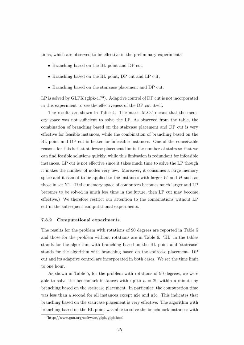
Table 6: Computational results on PP (without rotations)

staircase BL

name n time (s)† nodes time (s)† nodes

n2a 25 0.01 624 3.57 46,072

n2b 25 0.03 2274 57.15 764,406

n2c 25 0.01 283 170.17 2,210,939

n2d 25 0.00 115 45.51 644,484

n2e 25 0.09 6323 488.85 6,340,166

n3a 29 0.01 210 T.O. —

n3b 29 0.02 1163 T.O. —

n3c 29 0.05 6079 536.00 5,951,385

n3d 29 0.01 438 664.18 7,755,592

n3e 29 0.02 1380 1526.61 19,009,868

n4a 49 2743.31 138,563,048 T.O. —

n4b 49 280.16 19,305,123 T.O. —

n4c 49 T.O. — T.O. —

n4d 49 2188.01 128,560,407 T.O. —

n4e 49 2298.45 125,137,867 T.O. —†on a Pentium 4 (3GHz) with the time limit of 3600 seconds

n = 17 in reasonable time, but is less effective than branching based on the

staircase placement.

From Table 6, we can observe that branching based on the staircase placement

is also very effective for the case without rotations of 90 degrees; the algorithm

was able to solve four out of the five benchmark instances with 49 rectangles

within the time limit. The algorithm with branching based on the BL point was

able to solve the benchmark instances with n = 25 and three out of the five

instances with n = 29 within the time limit, but is less effective than branching

based on the staircase placement as is the case with rotations. Lesh et al. (2004)

also tested their algorithms on these benchmark instances. They used a PC with

Pentium 2.0GHz for the experiments. Their algorithm solved the five benchmark

instances with 17 rectangles rectangles within a second, the five instances with 25

rectangles under two minutes on average, and four out of the five instances with

29 rectangles under ten minutes on average. They also tested another branching

rule, and solved all the five instances with 29 rectangles. They did not test

the five benchmark instances with 49 rectangles. The CPU we used is about

1.5 times faster than that used in (Lesh et al. 2004), but even considering the

difference of the CPUs, our algorithm is very effective compared with the results

in (Lesh et al. 2004).

27

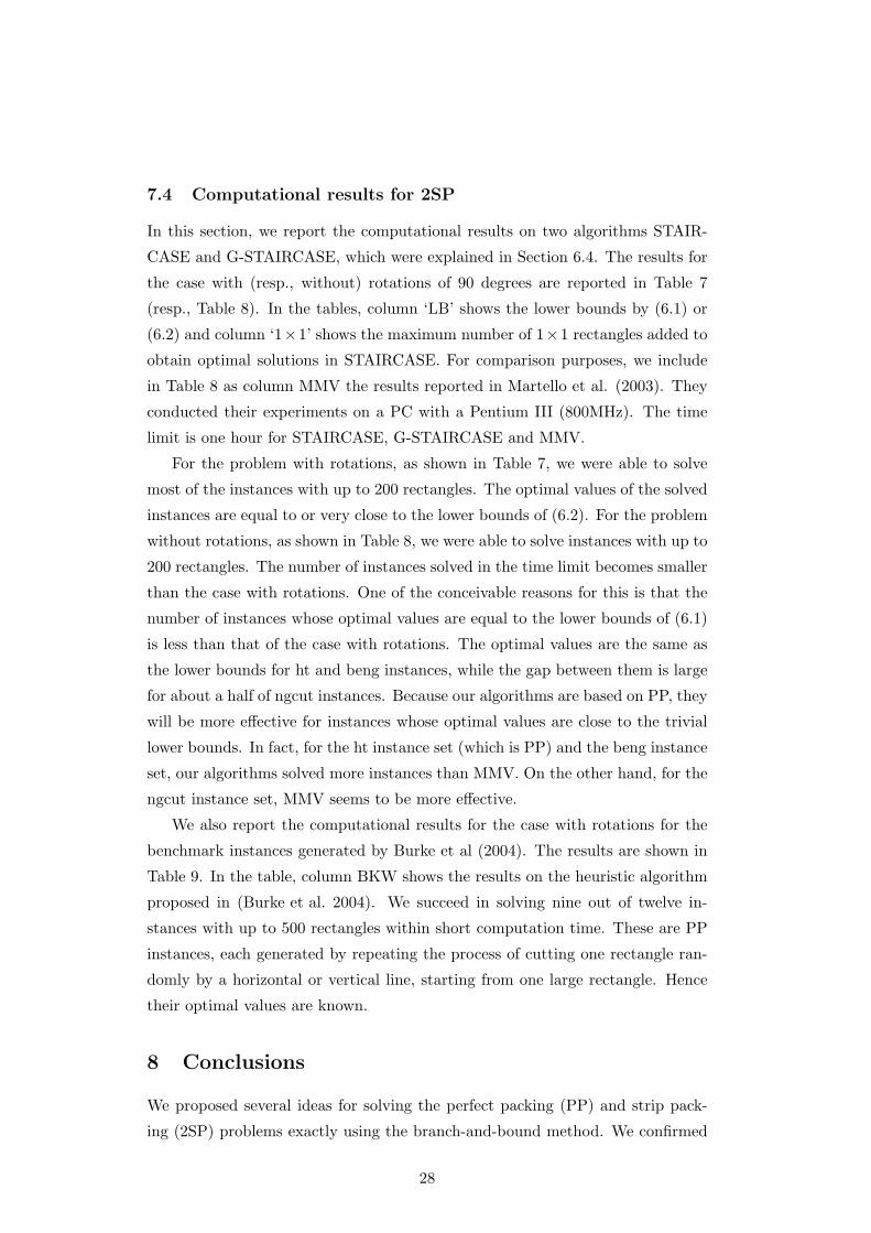
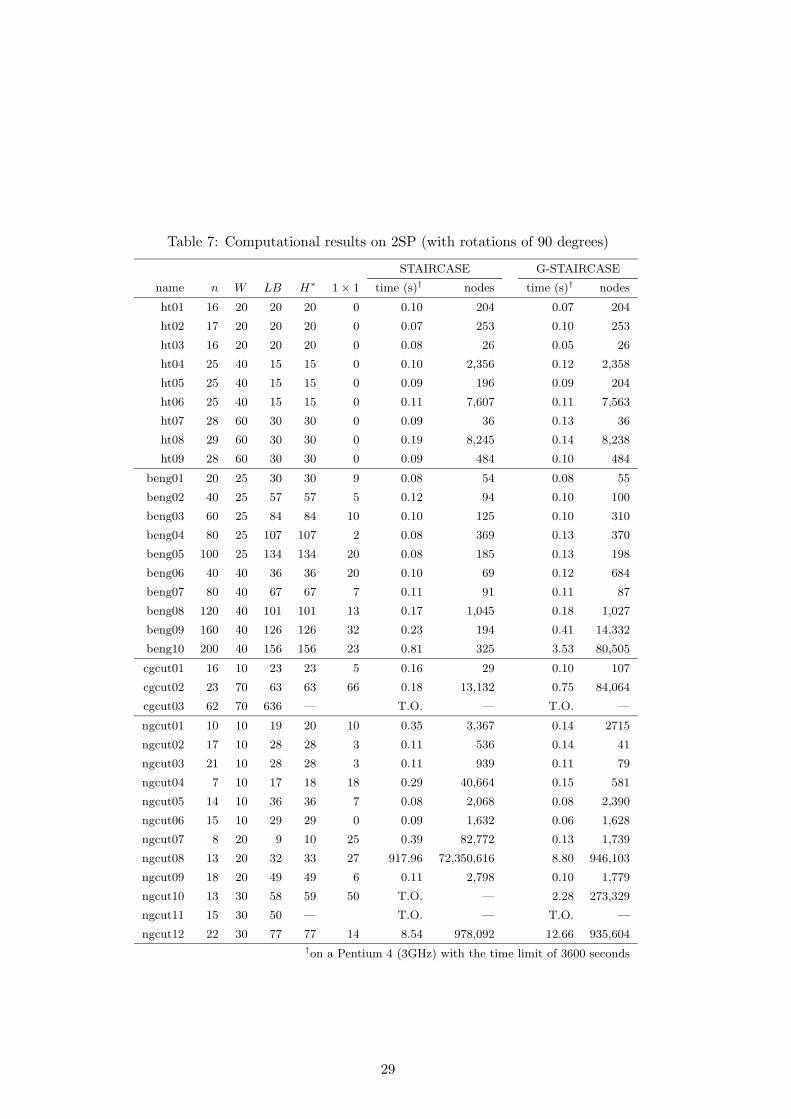
7.4 Computational results for 2SP

In this section, we report the computational results on two algorithms STAIR-

CASE and G-STAIRCASE, which were explained in Section 6.4. The results for

the case with (resp., without) rotations of 90 degrees are reported in Table 7

(resp., Table 8). In the tables, column ‘LB’ shows the lower bounds by (6.1) or

(6.2) and column ‘1×1’ shows the maximum number of 1×1 rectangles added to

obtain optimal solutions in STAIRCASE. For comparison purposes, we include

in Table 8 as column MMV the results reported in Martello et al. (2003). They

conducted their experiments on a PC with a Pentium III (800MHz). The time

limit is one hour for STAIRCASE, G-STAIRCASE and MMV.

For the problem with rotations, as shown in Table 7, we were able to solve

most of the instances with up to 200 rectangles. The optimal values of the solved

instances are equal to or very close to the lower bounds of (6.2). For the problem

without rotations, as shown in Table 8, we were able to solve instances with up to

200 rectangles. The number of instances solved in the time limit becomes smaller

than the case with rotations. One of the conceivable reasons for this is that the

number of instances whose optimal values are equal to the lower bounds of (6.1)

is less than that of the case with rotations. The optimal values are the same as

the lower bounds for ht and beng instances, while the gap between them is large

for about a half of ngcut instances. Because our algorithms are based on PP, they

will be more effective for instances whose optimal values are close to the trivial

lower bounds. In fact, for the ht instance set (which is PP) and the beng instance

set, our algorithms solved more instances than MMV. On the other hand, for the

ngcut instance set, MMV seems to be more effective.

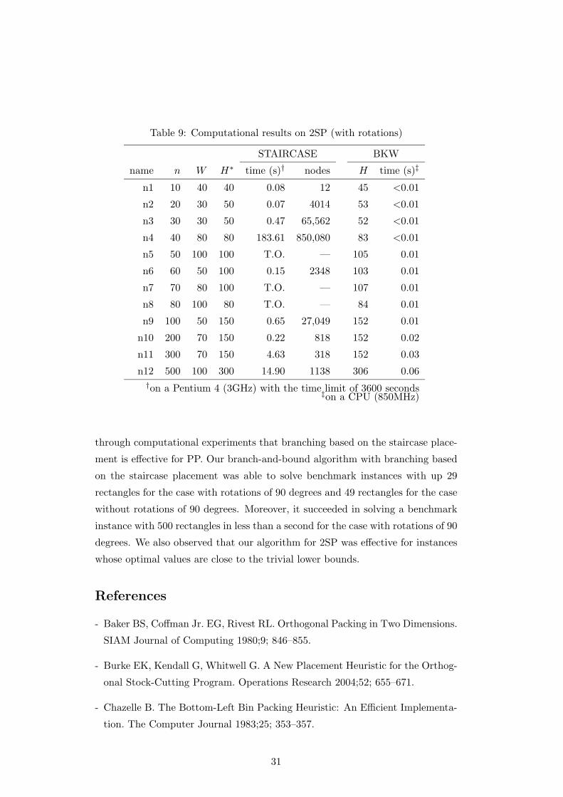
We also report the computational results for the case with rotations for the

benchmark instances generated by Burke et al (2004). The results are shown in

Table 9. In the table, column BKW shows the results on the heuristic algorithm

proposed in (Burke et al. 2004). We succeed in solving nine out of twelve in-

stances with up to 500 rectangles within short computation time. These are PP

instances, each generated by repeating the process of cutting one rectangle ran-

domly by a horizontal or vertical line, starting from one large rectangle. Hence

their optimal values are known.

8 Conclusions

We proposed several ideas for solving the perfect packing (PP) and strip pack-

ing (2SP) problems exactly using the branch-and-bound method. We confirmed

28

Table 7: Computational results on 2SP (with rotations of 90 degrees)

STAIRCASE G-STAIRCASE

name n W LB H∗ 1 × 1 time (s)† nodes time (s)† nodes

ht01 16 20 20 20 0 0.10 204 0.07 204

ht02 17 20 20 20 0 0.07 253 0.10 253

ht03 16 20 20 20 0 0.08 26 0.05 26

ht04 25 40 15 15 0 0.10 2,356 0.12 2,358

ht05 25 40 15 15 0 0.09 196 0.09 204

ht06 25 40 15 15 0 0.11 7,607 0.11 7,563

ht07 28 60 30 30 0 0.09 36 0.13 36

ht08 29 60 30 30 0 0.19 8,245 0.14 8,238

ht09 28 60 30 30 0 0.09 484 0.10 484

beng01 20 25 30 30 9 0.08 54 0.08 55

beng02 40 25 57 57 5 0.12 94 0.10 100

beng03 60 25 84 84 10 0.10 125 0.10 310

beng04 80 25 107 107 2 0.08 369 0.13 370

beng05 100 25 134 134 20 0.08 185 0.13 198

beng06 40 40 36 36 20 0.10 69 0.12 684

beng07 80 40 67 67 7 0.11 91 0.11 87

beng08 120 40 101 101 13 0.17 1,045 0.18 1,027

beng09 160 40 126 126 32 0.23 194 0.41 14,332

beng10 200 40 156 156 23 0.81 325 3.53 80,505

cgcut01 16 10 23 23 5 0.16 29 0.10 107

cgcut02 23 70 63 63 66 0.18 13,132 0.75 84,064

cgcut03 62 70 636 — T.O. — T.O. —

ngcut01 10 10 19 20 10 0.35 3,367 0.14 2715

ngcut02 17 10 28 28 3 0.11 536 0.14 41

ngcut03 21 10 28 28 3 0.11 939 0.11 79

ngcut04 7 10 17 18 18 0.29 40,664 0.15 581

ngcut05 14 10 36 36 7 0.08 2,068 0.08 2,390

ngcut06 15 10 29 29 0 0.09 1,632 0.06 1,628

ngcut07 8 20 9 10 25 0.39 82,772 0.13 1,739

ngcut08 13 20 32 33 27 917.96 72,350,616 8.80 946,103

ngcut09 18 20 49 49 6 0.11 2,798 0.10 1,779

ngcut10 13 30 58 59 50 T.O. — 2.28 273,329

ngcut11 15 30 50 — T.O. — T.O. —

ngcut12 22 30 77 77 14 8.54 978,092 12.66 935,604†on a Pentium 4 (3GHz) with the time limit of 3600 seconds

29

Table 8: Computational results on 2SP (without rotations)

STAIRCASE G-STAIRCASE MMV

name n W LB H∗ 1 × 1 time (s)† nodes time (s)† nodes time (s)‡

ht01 16 20 20 20 0 0.10 52 0.07 52 10.84

ht02 17 20 20 20 0 0.12 1,325 0.07 1,315 623.53

ht03 16 20 20 20 0 0.08 22 0.10 22 500.75

ht04 25 40 15 15 0 0.08 3,547 0.11 3,545 8.26

ht05 25 40 15 15 0 0.09 599 0.06 599 20.29

ht06 25 40 15 15 0 0.11 2,215 0.06 2,212 16.94

ht07 28 60 30 30 0 0.12 1,340 0.10 1,340 T.O.

ht08 29 60 30 30 0 71.40 3,030,967 76.97 2,957,065 T.O.

ht09 28 60 30 30 0 0.10 116 0.13 116 0.00

beng01 20 25 30 30 9 0.53 74,209 0.93 95,784 511.58

beng02 40 25 57 57 5 1.13 94,169 22.89 463,205 T.O.

beng03 60 25 84 84 10 0.94 40,653 0.32 10,311 T.O.

beng04 80 25 107 107 2 0.25 5,309 T.O. — T.O.

beng05 100 25 134 134 20 0.15 4,345 0.31 8,530 500.62

beng06 40 40 36 36 20 0.07 204 0.29 25,369 T.O.

beng07 80 40 67 67 7 0.33 9,021 0.18 802 0.56

beng08 120 40 101 101 13 1.36 33,596 2.67 77,150 500.54

beng09 160 40 126 126 32 0.42 7,047 2.38 39,467 0.03

beng10 200 40 156 156 23 2.86 6,977 6.52 101,671 0.03

cgcut01 16 10 23 23 5 0.10 3,789 0.12 3,578 11.48

cgcut02 23 70 63 — T.O. — T.O. — T.O.

cgcut03 62 70 636 — T.O. — T.O. — T.O.

ngcut01 10 10 19 23 40 2080.04 257,058,531 0.39 23,854 0.05

ngcut02 17 10 28 29 13 T.O. — T.O. — 11.31

ngcut03 21 10 28 28 3 0.09 184 0.10 152 27.01

ngcut04 7 10 17 20 38 3.63 766,572 0.14 106 0.00

ngcut05 14 10 36 36 7 0.11 56 0.07 83 0.00

ngcut06 15 10 29 31 20 T.O. — 147.31 4,423,772 727.20

ngcut07 8 20 20 20 225 T.O. — 0.10 16 0.00

ngcut08 13 20 32 33 27 30.51 3,911,039 0.50 39,291 53.09

ngcut09 18 20 49 50 26 T.O. — 1971.64 42,196,600 T.O.

ngcut10 13 30 58 80 680 T.O. — 113.98 12,642,065 0.18

ngcut11 15 30 50 52 77 T.O. — 7.71 573,883 483.01

ngcut12 22 30 77 87 314 T.O. — T.O. — 0.00†on a Pentium 4 (3GHz) with the time limit of 3600 seconds‡on a Pentium III (800MHz) with the time limit of 3600 seconds

30

Table 9: Computational results on 2SP (with rotations)

STAIRCASE BKW

name n W H∗ time (s)† nodes H time (s)‡

n1 10 40 40 0.08 12 45 <0.01

n2 20 30 50 0.07 4014 53 <0.01

n3 30 30 50 0.47 65,562 52 <0.01

n4 40 80 80 183.61 850,080 83 <0.01

n5 50 100 100 T.O. — 105 0.01

n6 60 50 100 0.15 2348 103 0.01

n7 70 80 100 T.O. — 107 0.01

n8 80 100 80 T.O. — 84 0.01

n9 100 50 150 0.65 27,049 152 0.01

n10 200 70 150 0.22 818 152 0.02

n11 300 70 150 4.63 318 152 0.03

n12 500 100 300 14.90 1138 306 0.06†on a Pentium 4 (3GHz) with the time limit of 3600 seconds‡on a CPU (850MHz)

through computational experiments that branching based on the staircase place-

ment is effective for PP. Our branch-and-bound algorithm with branching based

on the staircase placement was able to solve benchmark instances with up 29

rectangles for the case with rotations of 90 degrees and 49 rectangles for the case

without rotations of 90 degrees. Moreover, it succeeded in solving a benchmark

instance with 500 rectangles in less than a second for the case with rotations of 90

degrees. We also observed that our algorithm for 2SP was effective for instances

whose optimal values are close to the trivial lower bounds.

References

- Baker BS, Coffman Jr. EG, Rivest RL. Orthogonal Packing in Two Dimensions.

SIAM Journal of Computing 1980;9; 846–855.

- Burke EK, Kendall G, Whitwell G. A New Placement Heuristic for the Orthog-

onal Stock-Cutting Program. Operations Research 2004;52; 655–671.

- Chazelle B. The Bottom-Left Bin Packing Heuristic: An Efficient Implementa-

tion. The Computer Journal 1983;25; 353–357.

31

- Hopper E, Turton BCH. An Empirical Investigation of Meta-Heuristic and

Heuristic Algorithms for a 2D Packing Problems. European Journal of Opera-

tional Research 2000;128; 34–57.

- Hopper E, Turton BCH. A Review of the Application of Meta-Heuristic Algo-

rithms to 2D Strip Packing Problems. Artificial Intelligence Review 2001;16;

257–300.

- Ibaraki T. JC Baltzer AG: Enumerative Approaches to Combinatorial Opti-

mization. Annals of Operations Research, vol.10 and 11; Basel; 1987.

- Imahori S, Yagiura M, Ibaraki T. Local Search Algorithms for the Rectan-

gle Packing Problem with General Spatial Costs. Mathematical Programming

Series B 2003;97; 543–569.

- Imahori S, Yagiura M, Ibaraki T. Improved Local Search Algorithms for the

Rectangle Packing Problem with General Spatial Costs. European Journal of

Operational Research 2005;167; 48–67.

- Jakobs S. On Genetic Algorithms for the Packing of Polygons. European Jour-

nal of Operational Research 1996;88; 165–181.

- Lesh N, Marks J, McMahon A, Mitzenmacher M. Exhaustive Approaches to 2D

Rectangular Perfect Packings. Information Processing Letters 2004;90; 7–14.

- Liu D, Teng H. An Improved BL-Algorithm for Genetic Algorithm of the Or-

thogonal Packing of Rectangles. European Journal of Operational Research

1999;112; 413–419.

- Martello S, Toth P. John Wiley & Sons: Knapsack Problems – Algorithms and

Computer Implementations. Chichester-New York; 1990.

- Martello S, Pisinger D, Vigo D. The Three Dimensional Bin Packing Problem.

Operations Research 2000;48; 256–267.

- Martello S, Monaci M, Vigo D. An Exact Approach to the Strip-Packing Prob-

lem. INFORMS Journal on Computing 2003;15; 310–319.

- Matsuda Y. The fourth Supercomputer Programming Contest for High School

Students at Tokyo Institute of Technology. Sugaku Seminar (Mathematics Sem-

inar) 1998;12; 40–43, in Japanese.

32

- Murata H, Fujiyoshi K, Nakatate S, Kajitani Y. VLSI Module Placement Based

on Rectangle-Packing by the Sequence-Pair. IEEE Transactions on Computers

1996;15–12; 1518–1524.

- Turek J, Wolf J, Yu P. Approximate algorithms for scheduling parallelizable

tasks. Proceedings of the fourth Annual ACM Symposium on Parallel Algo-

rithms and Architectures 1992; 323–332.

33